DIGITAL HEARING AIDS

16 April 2009

James M. Kates

Research Fellow, GN ReSound A/S

AdjointFaculty, CU Boulder

jkates@

gnresound.dk

2

Contents

•Hearing and hearing loss

•Hearing aid types and processing constraints

•Dynamic-range compression

•Noise suppression

•Feedback cancellation

•Microphones and arrays

•List of additional areas

•Conclusions

Hearing and

Hearing Loss

4

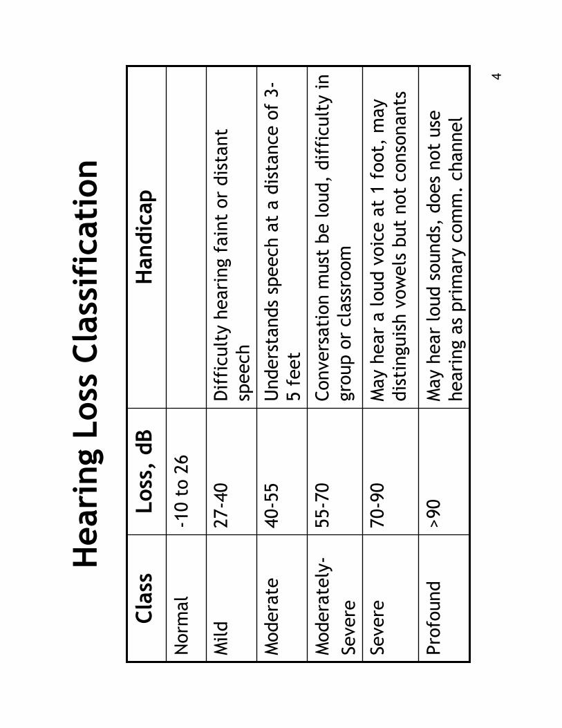
Hearing Loss Classification

May hear loud sounds, does not use

hearing as primary comm. channel

>90

Profound

May hear a loud voice at 1 foot, may

distinguish vowels but not consonants

70-90

Severe

Conversation must be loud, difficulty in

group or classroom

55-70

Moderately-

Severe

Understands speech at a distance of 3-

5 feet

40-55

Moderate

Difficulty hearing faint or distant

speech

27-40

Mild

-10 to 26

Norm

al

Handicap

Loss, dB

Class

5

6

7

8

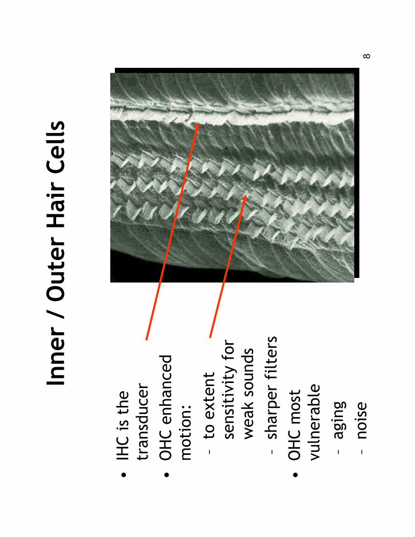
Inner / Outer Hair Cells

•IHC is the

transducer

•OHC enhanced

motion:

–to extent

sensitivity for

weak sounds

–sharper filters

•OHC most

vulnerable

–aging

–noise

9

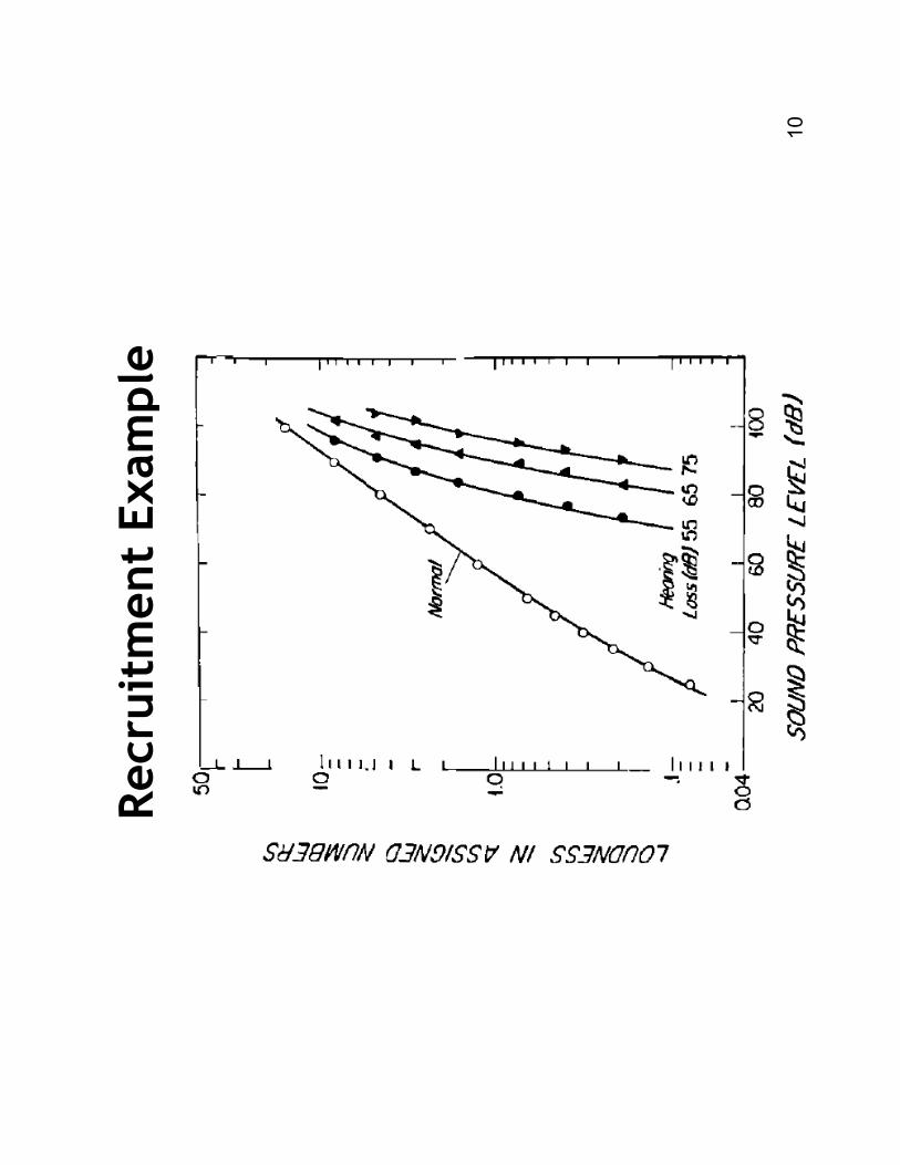
Recruitment

•Reduced dynamic range in impaired ear

–Healthy cochlea has instantaneous compression

–Loss of active OHC gain mechanism in impairment

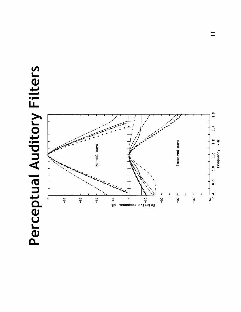
–Reduced cochlear gain, increased filter bandwidth

–Impaired ear is more linear than healthy ear

–Recruitment = abnorm

al rapid increase in loudness

–Loudness at 100 dB SPL approx equal

•Compression

–Compensate for OHC damage

–High face validity

–Benefits in practice are mixed

10

Recruitment Example

11

Perceptual Auditory Filters

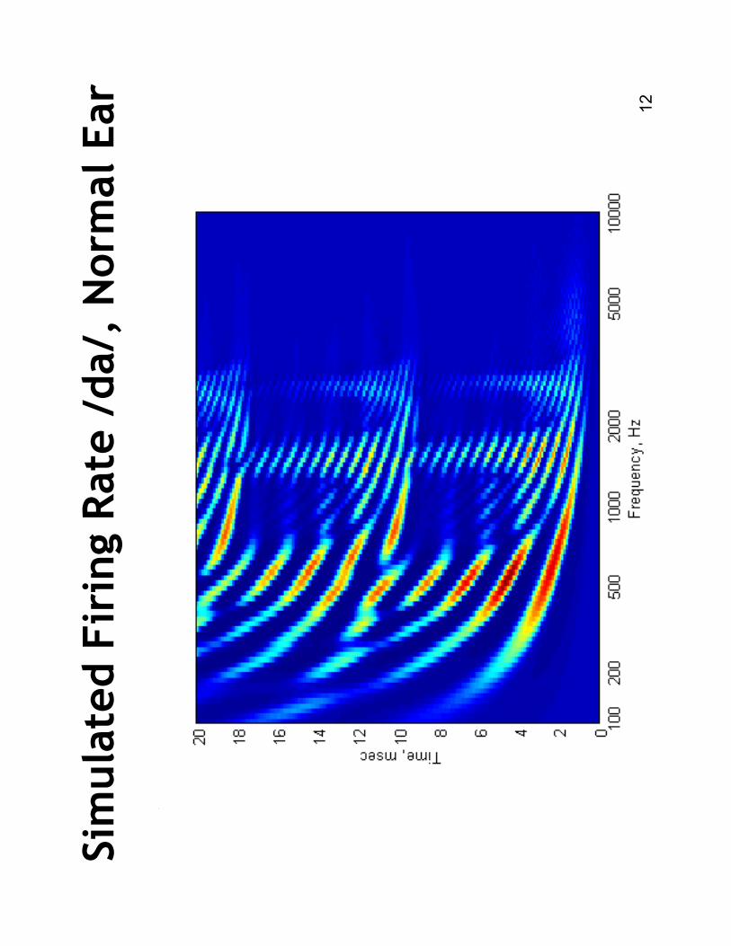
12

Simulated Firing Rate /da/, Norm

al Ear

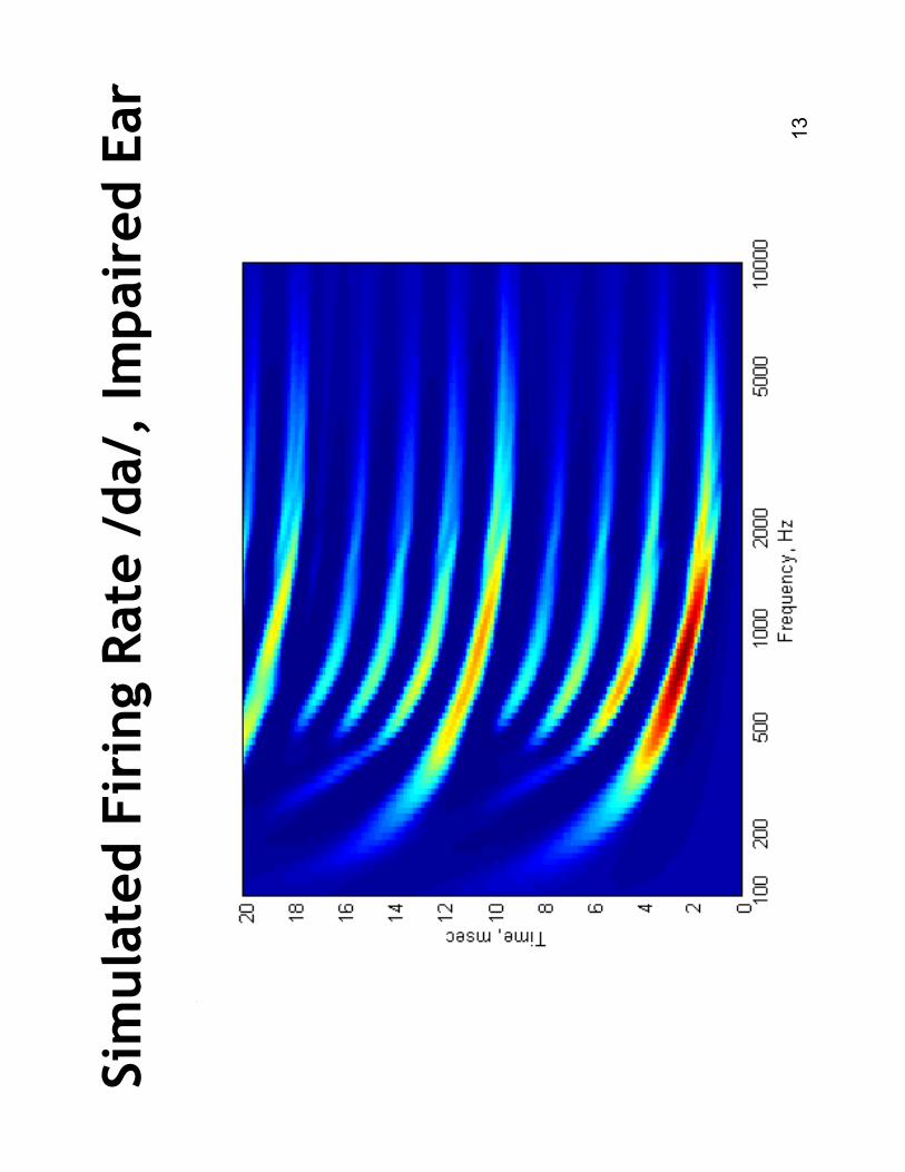
13

Simulated Firing Rate /da/, Impaired Ear

14

Hearing Loss Conclusions

•Outer hair-cell damage

–Shift in auditory threshold

–Recruitment: Impaired system is more linear

–Broader auditory filters

•Inner hair-cell damage

–Shift in auditory threshold

–“Dead regions”

with no response

•Can not perceive low-intensity speech sounds

•Difficulty in noise and reverberation

Hearing Aid Types and

Processing Constraints

16

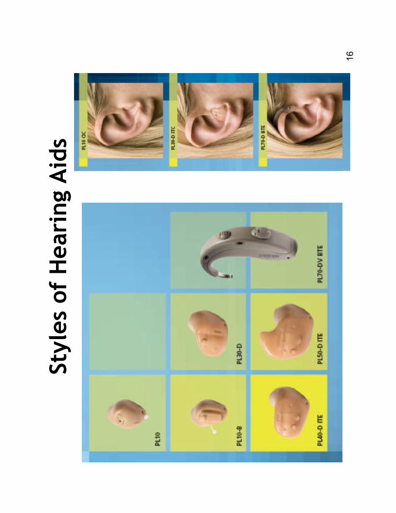
Styles of Hearing Aids

17

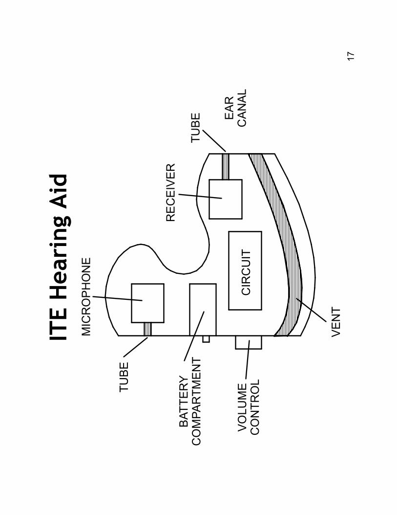
ITE Hearing Aid

MIC

RO

PH

ON

E

TU

BE

BATTER

YC

OM

PAR

TM

EN

T

VO

LU

ME

CO

NTR

OL

REC

EIV

ER

TU

BE

CIR

CU

IT

VEN

T

EAR

CAN

AL

18

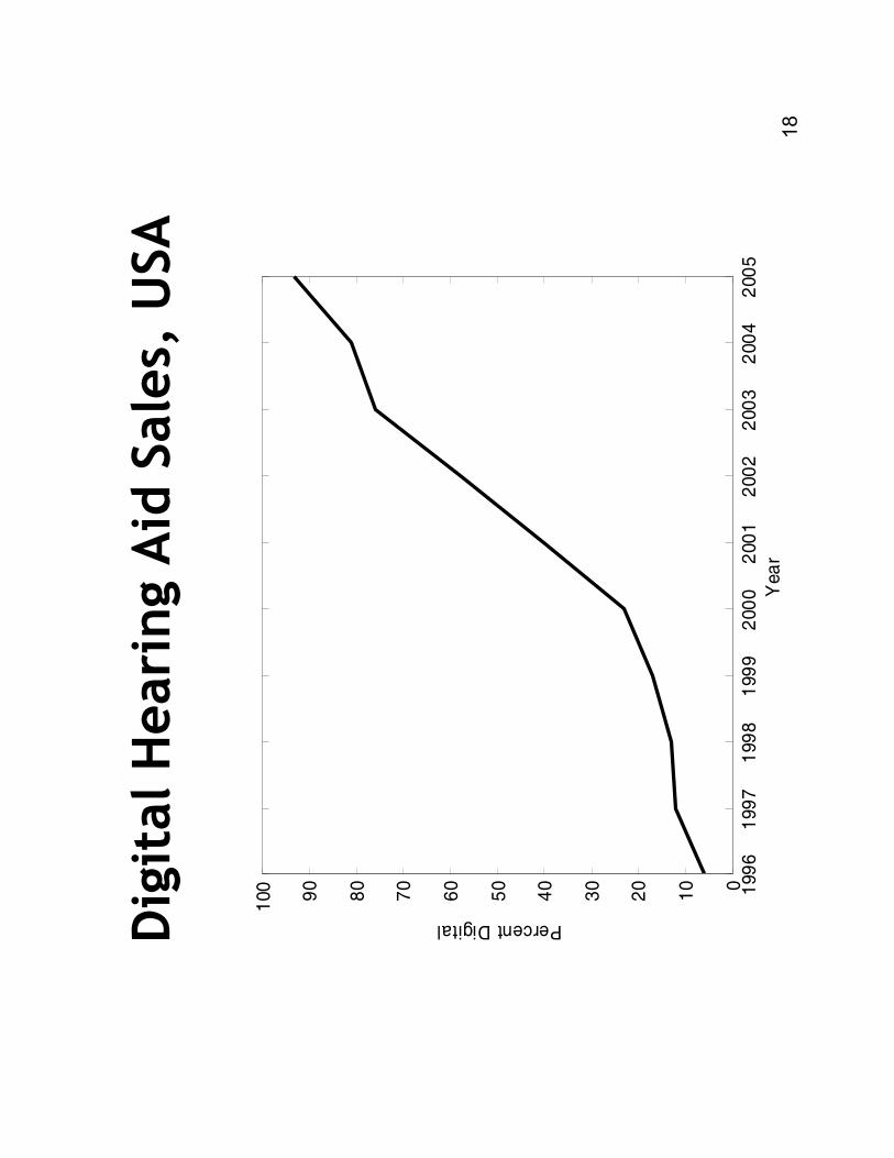
Digital Hearing Aid Sales, USA

199

61

99

71

99

81

99

92

00

02

00

12

00

22

00

32

00

42

00

50

10

20

30

40

50

60

70

80

90

100

Yea

r

Percent Digital

19

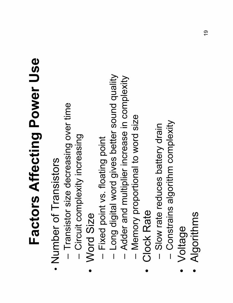
Factors Affecting Power Use

•N

um

ber of Tra

nsis

tors

–Tra

nsis

tor siz

e d

ecre

asin

g o

ver tim

e

–C

ircuit c

om

ple

xity incre

asin

g

•W

ord

Siz

e–

Fix

ed p

oin

t vs. floating p

oin

t

–Long d

igital w

ord

giv

es b

etter sound q

ualit

y

–Adder and m

ultip

lier in

cre

ase in c

om

ple

xity

–M

em

ory

pro

portio

nal to

word

siz

e

•C

lock R

ate

–Slo

w rate

reduces b

attery

dra

in

–C

onstrain

s a

lgorith

m c

om

ple

xity

•Voltage

•Alg

orith

ms

20

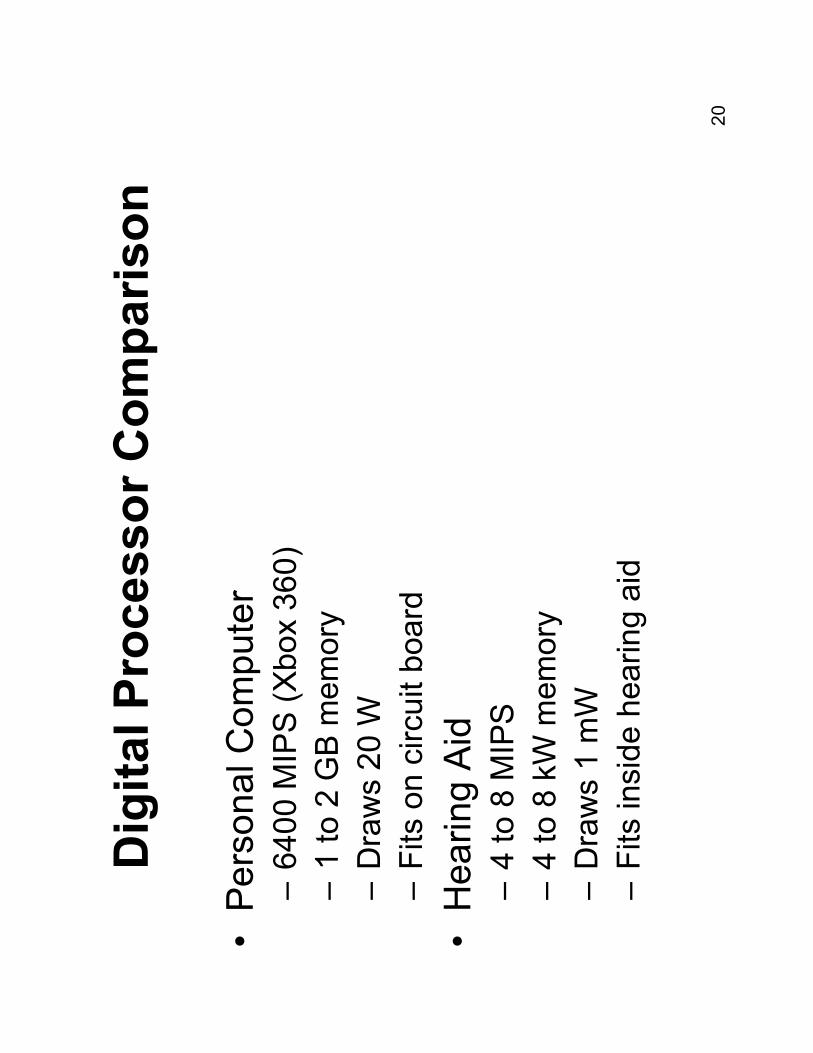
Digital Processor Comparison

•Pers

onal C

om

pute

r–

6400 M

IPS (Xbox 3

60)

–1 to 2

GB m

em

ory

–D

raw

s 2

0 W

–Fits o

n c

ircuit b

oard

•H

earing A

id–

4 to 8

MIP

S

–4 to 8

kW

mem

ory

–D

raw

s 1

mW

–Fits insid

e h

earing a

id

21

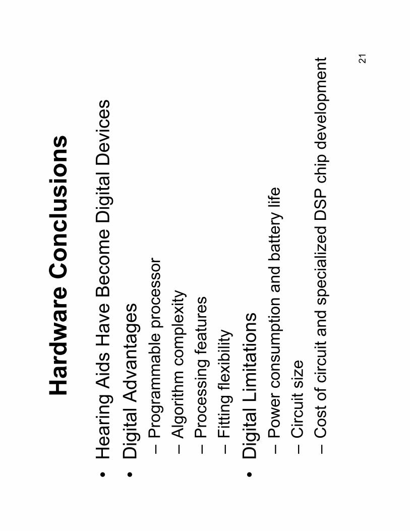
Hardware Conclusions

•H

earing A

ids H

ave B

ecom

e D

igital D

evic

es

•D

igital Advanta

ges

–Pro

gra

mm

able

pro

cessor

–Alg

orith

m c

om

ple

xity

–Pro

cessin

g featu

res

–Fitting fle

xib

ility

•D

igital Lim

itations

–Pow

er consum

ption a

nd b

attery

life

–C

ircuit s

ize

–C

ost of circuit a

nd s

pecia

lized D

SP c

hip

develo

pm

ent

Dynamic-Range

Compression

23

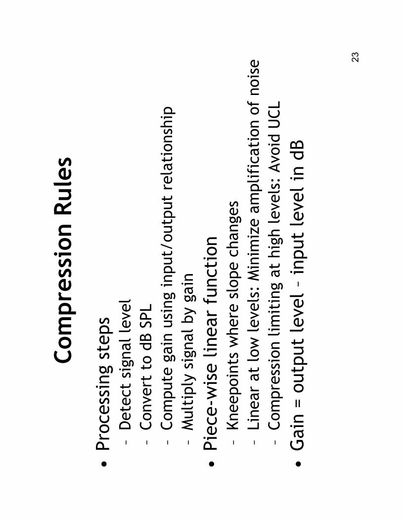
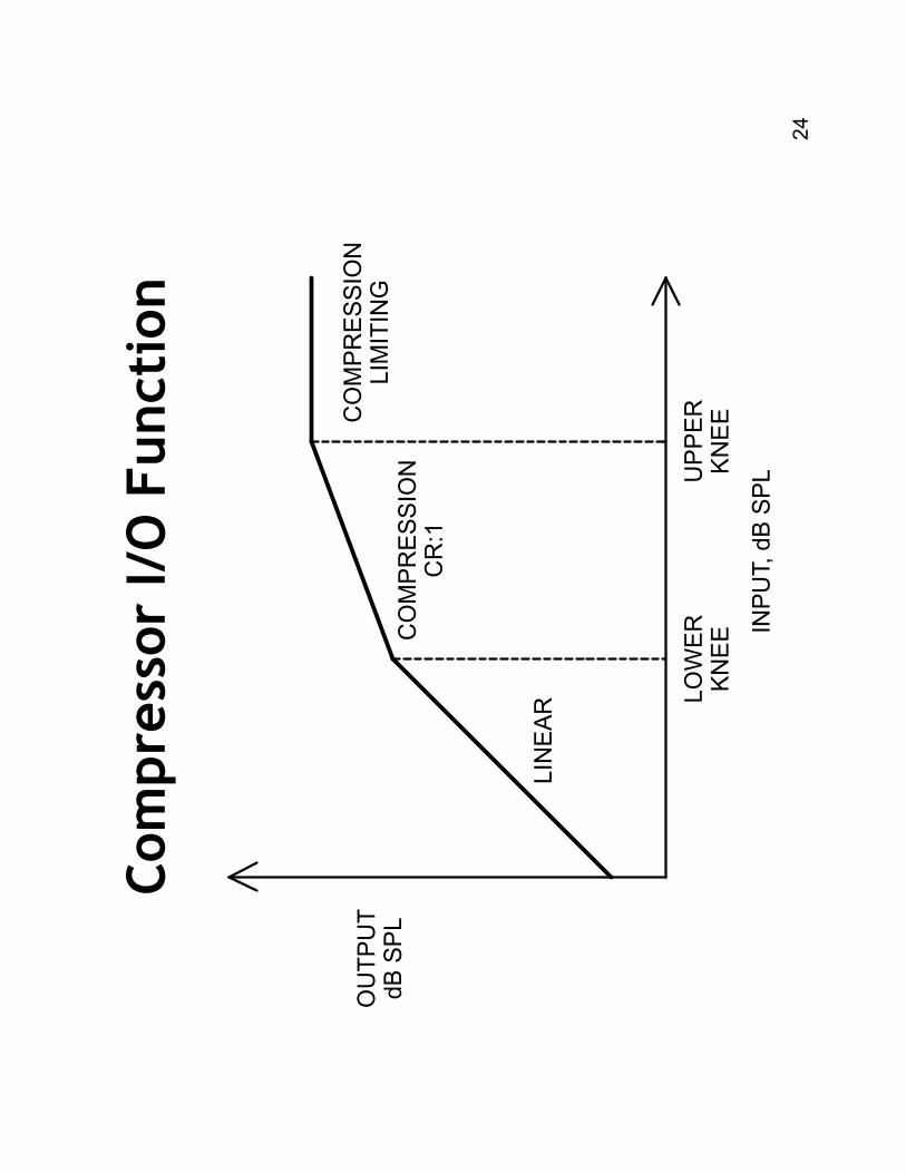
Compression Rules

•Processing steps

–Detect signal level

–Convert to dB SPL

–Compute gain using input/output relationship

–Multiply signal by gain

•Piece-wise linear function

–Kneepointswhere slope changes

–Linear at low levels: Minimize amplification of noise

–Compression limiting at high levels: Avoid UCL

•Gain = output level –input level in dB

24

Compressor I/O Function

LIN

EA

R

CO

MP

RE

SS

ION

CR

:1

CO

MP

RE

SS

ION

LIM

ITIN

G

LO

WE

RK

NE

EU

PP

ER

KN

EE

INP

UT, dB

SP

L

OU

TP

UT

dB

SP

L

25

Envelope Detection

•Track incoming signal level

•Response depends on sign of signal changes

–Rapid response to increases in signal level (attack)

–Slower response to decreases (release)

–Defined by attack and release time constants

•Fast attack

–Signals tend to increase more rapidly than decrease

–Prevent over-amplification of large sudden increase

•Slow release

–Rapid gain changes cause audible modulation

–Hold gain relatively constant during syllables

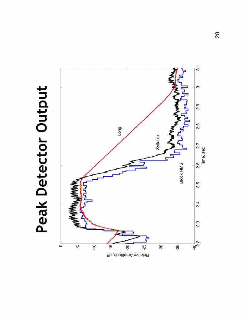
26

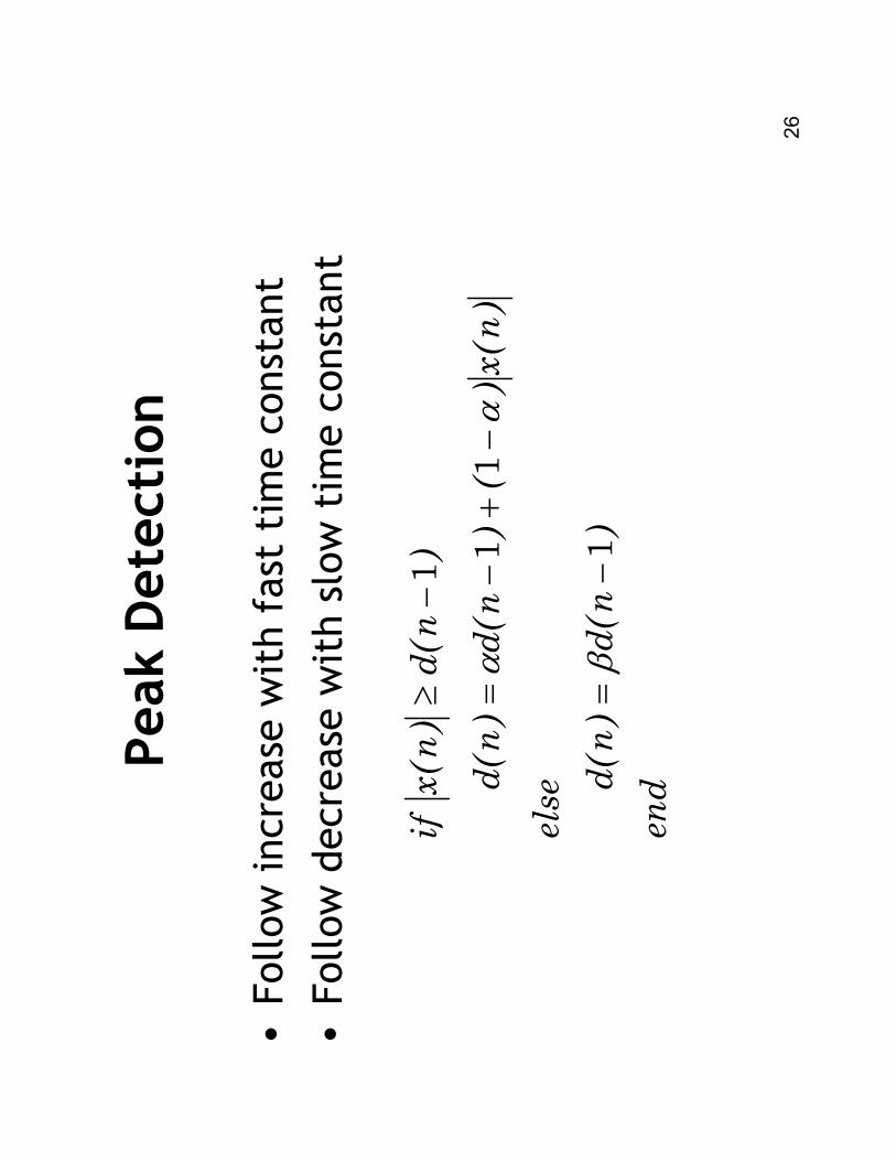
Peak Detection

•Follow increase with fast time constant

•Follow decrease with slow time constant

end

)n(

d)n(

d

else

)n(

x)

()

n(d

)n(

d

)n(

d)n(

xif

1

11

1 −=

−+

−=

−≥

β

αα

27

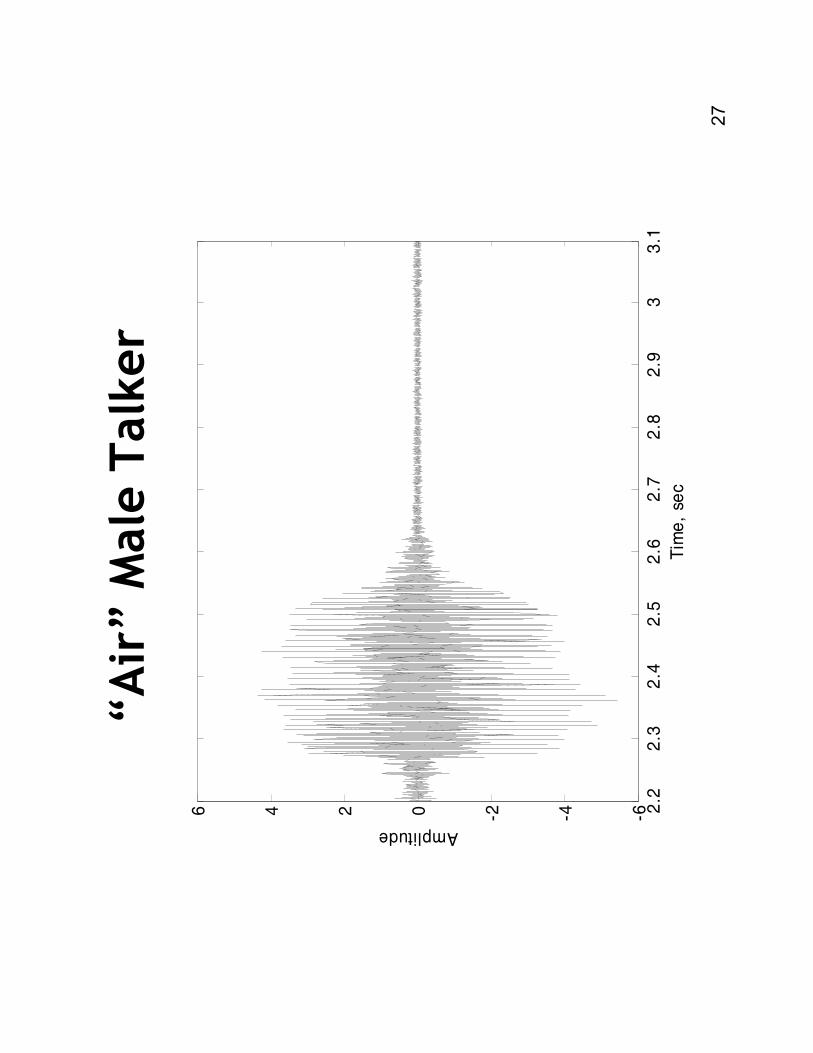
“Air”Male Talker

2.2

2.3

2.4

2.5

2.6

2.7

2.8

2.9

33

.1-6-4-20246

Tim

e,

sec

Amplitude

28

Peak Detector Output

2.2

2.3

2.4

2.5

2.6

2.7

2.8

2.9

33.1

-40

-35

-30

-25

-20

-15

-10-50

Tim

e,

sec

Relative Amplitude, dB

Long

Sylla

bic

Blo

ck R

MS

29

Multichannel Compression

•Frequency analysis

–Filter bank

–FFT

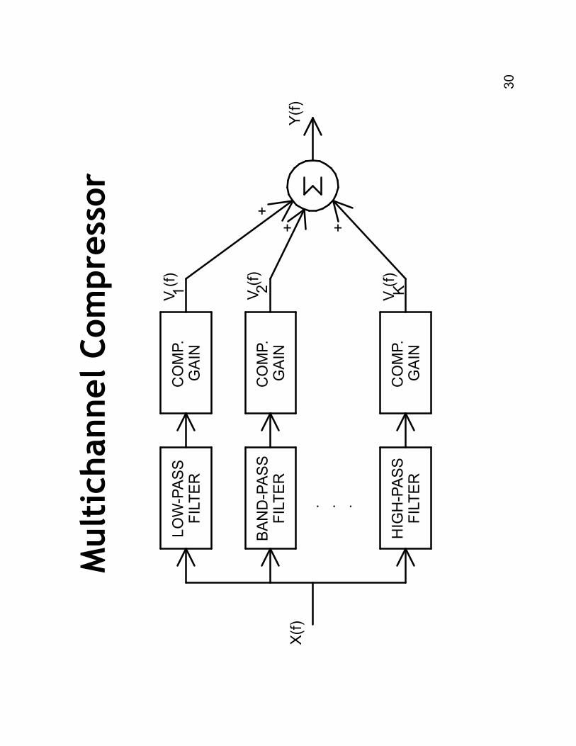
•Filter bank

–Auditory frequency spacing

–Independent compression in each frequency band

–Gain set in response to preceding signal level

–Response to signal change depends on time

constants

30

Multichannel Compressor

LO

W-P

AS

SFIL

TE

R

BA

ND

-PA

SS

FIL

TE

R

HIG

H-P

AS

SFIL

TE

R

CO

MP.

GA

IN

CO

MP.

GA

IN

CO

MP.

GA

IN

+

+ +

Y(f)

X(f)

. . .

V (f)

V (f)

V (f)

1 2 K

31

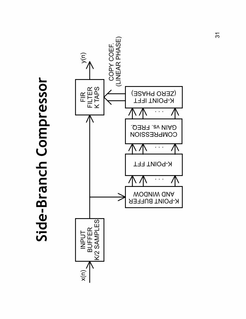
Side-Branch Compressor

y(n

)x(n

)IN

PU

TB

UFFE

RK

/2 S

AM

PLES

FIR

FIL

TE

RK

TA

PS

K-POINT FFT

COMPRESSIONGAIN vs. FREQ.

K-POINT IFFT(ZERO PHASE)

. .....

CO

PY C

OE

F.

(LIN

EA

R P

HA

SE)

K-POINT BUFFERAND WINDOW

...

32

Frequency W

arping

•FFT problems

–Uniform

frequency spacing

–Resolution at low frequencies is poor

–Need long delay to get good low-frequency analysis

•Goals of frequency warping

–Auditory frequency analysis

–Reduced group delay

–Reasonable computational requirements

•Want group delay < 10 msec

•Used in GN ReSound products

33

Warped Filter Structure

•Replace unit delays with all-pass filters

–FIR filter sums outputs at different delays

–Cascade of all-pass filters for cascade of unit delays

–Warped FIR sums outputs of all-pass filters

•Effects of the all-pass filters

–Low frequencies delayed from filter to filter

–Separation between filtered samples at low

frequencies > unit sample

–Separation at high frequencies < unit sample

34

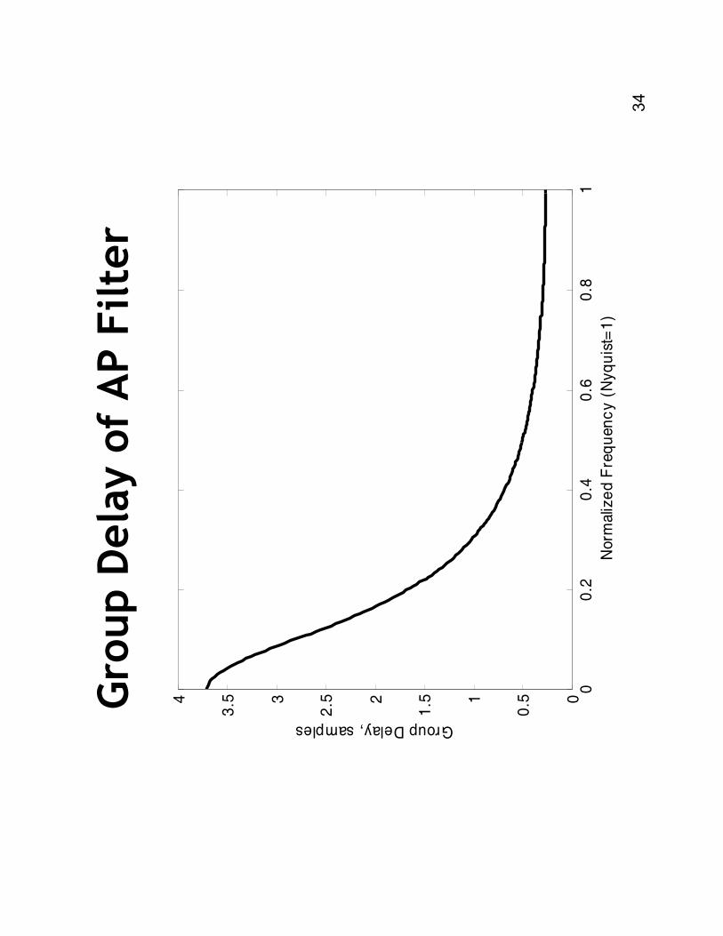
Group Delay of AP Filter

00

.20

.40

.60

.81

0

0.51

1.52

2.53

3.54

Norm

aliz

ed F

req

uen

cy

(N

yq

uis

t=1

)

Group Delay, samples

35

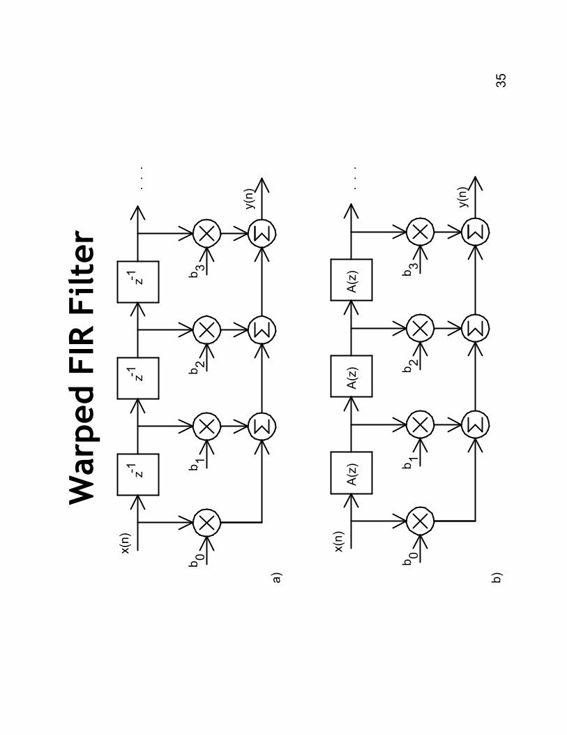
Warped FIR Filter

. . .

zz

zx(n

)

y(n

)

bb

bb

-1-1

-1

01

23

x(n

)

y(n

)

bb

bb

01

23

A(z

)A

(z)

A(z

). . .

a)

b)

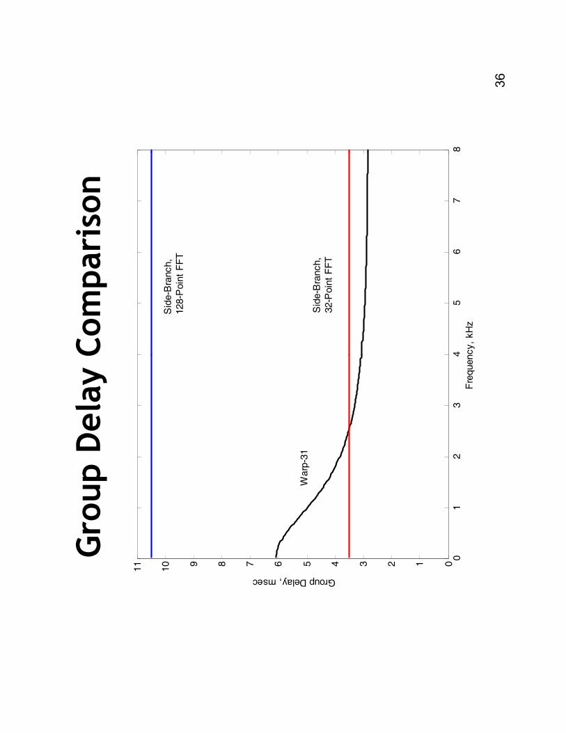
36

Group Delay Comparison

01

23

45

67

80123456789

10

11

Fre

quency,

kH

z

Group Delay, msec

Warp

-31

Sid

e-B

ranch,

32-P

oin

t F

FT

Sid

e-B

ranch,

128-P

oin

t F

FT

37

Warped Compressor Example

•Input

•Sampling rate

22.05 kHz

•16 bits

•23-band compressor

•Atttime=5 msec

•Reltime=70 msec

•CR=2:1 all bands

•Input at 65 dB SPL

38

Compression Conclusions

•Helps at low signal levels

•Compression ratio

–Generally prefer CR < 2:1

–Want lower CR as noise level increases

–Comp preferred if residual dynamic range < 30 dB

•Number of Channels

–No clear benefit to increasing the number of bands

–One channel shows sm

all benefit compared to multi

–Compressor co-modulates noise to match speech

Noise Suppression

40

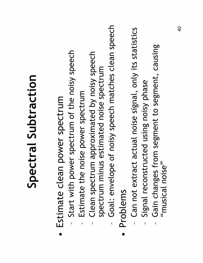
Spectral Subtraction

•Estimate clean power spectrum

–Start with power spectrum of the noisy speech

–Estimate the noise power spectrum

–Clean spectrum approximated by noisy speech

spectrum minus estimated noise spectrum

–Goal: envelope of noisy speech matches clean speech

•Problems

–Can not extract actual noise signal, only its statistics

–Signal reconstructed using noisy phase

–Gain changes from segment to segment, causing

“musical noise”

41

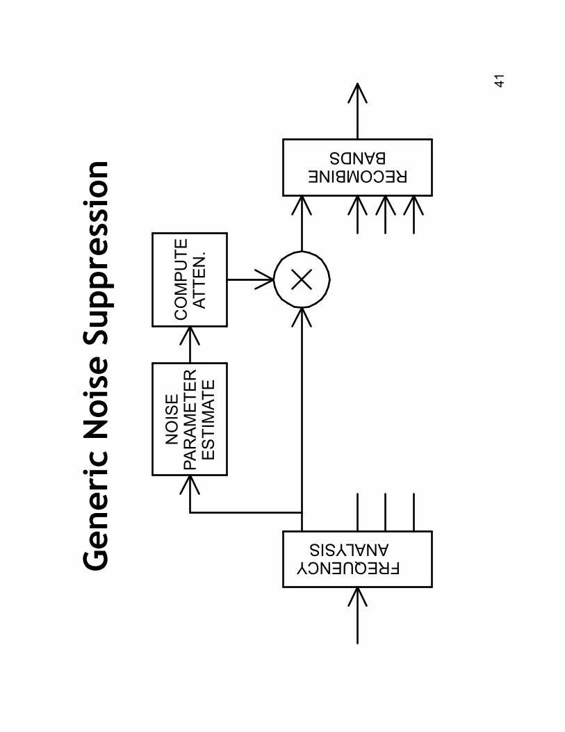
Generic Noise Suppression

NO

ISE

PA

RA

ME

TE

RE

STIM

ATE

CO

MP

UTE

ATTE

N.

FREQUENCYANALYSIS

RECOMBINEBANDS

42

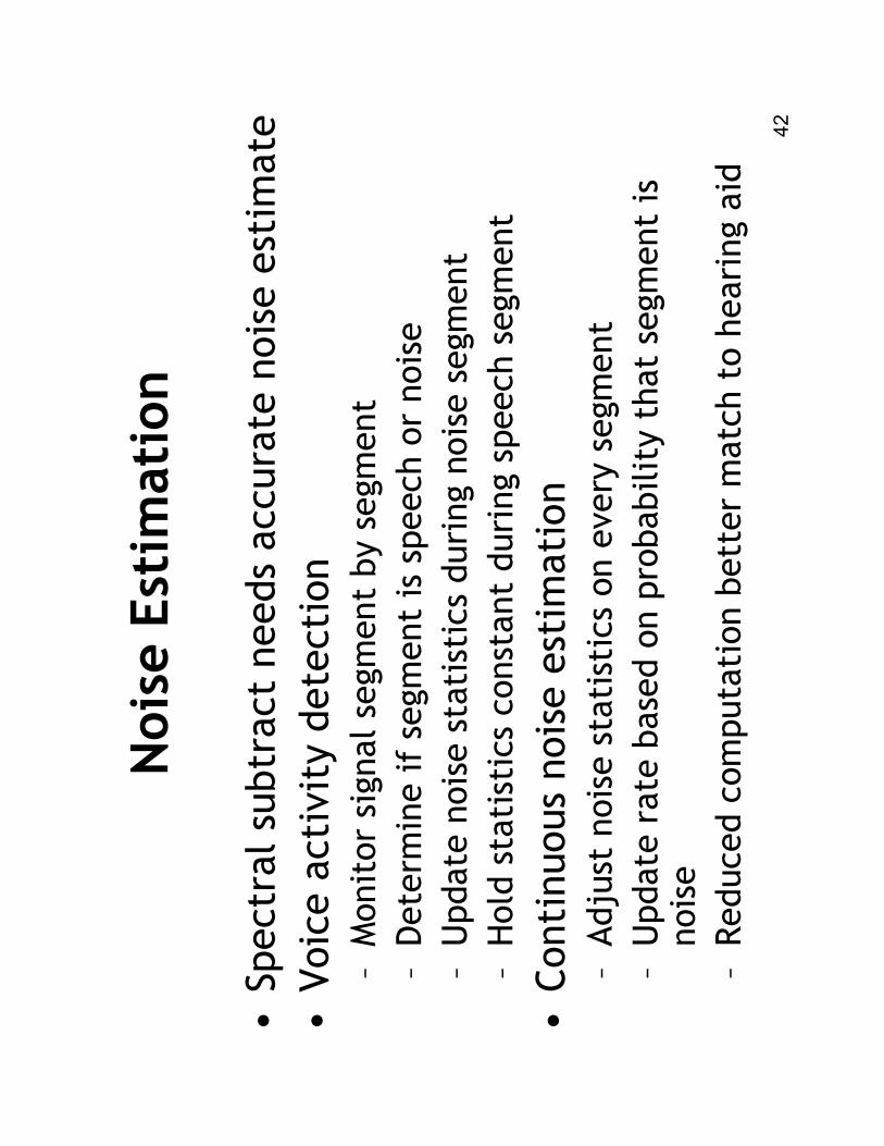
Noise Estimation

•Spectral subtract needs accurate noise estimate

•Voice activity detection

–Monitor signal segment by segment

–Determ

ine if segment is speech or noise

–Update noise statistics during noise segment

–Hold statistics constant during speech segment

•Continuous noise estimation

–Adjust noise statistics on every segment

–Update rate based on probability that segment is

noise

–Reduced computation better match to hearing aid

43

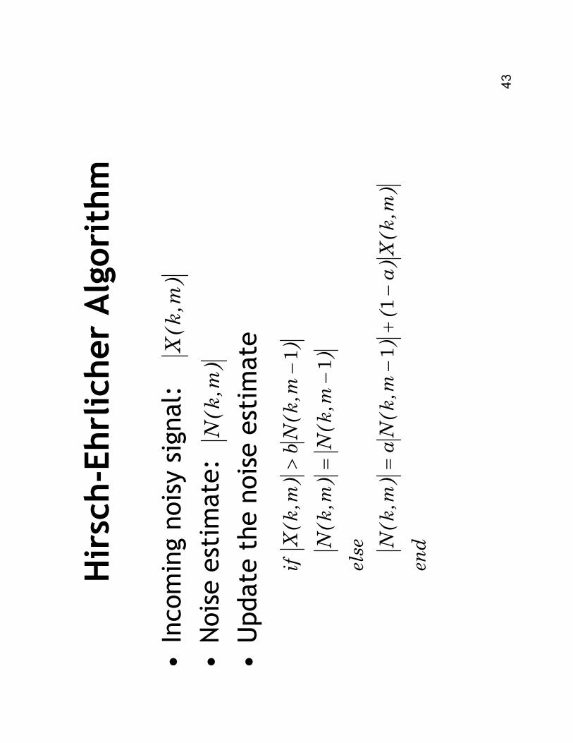
Hirsch-EhrlicherAlgorithm

•Incoming noisy signal:

•Noise estimate:

•Update the noise estimate

)m,

k(

X

)m,

k(

N

end

)m,

k(

X)a

()

m,k(

Na

)m,

k(

N

else

)m,

k(

N)

m,k(

N

)m,

k(

Nb

)m,

k(

Xif

−+

−=

−=

−>

11

1

1

44

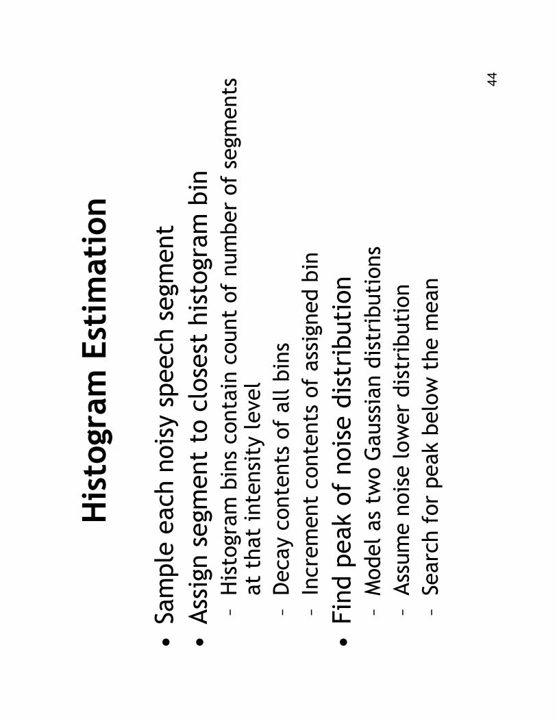
Histogram Estimation

•Sample each noisy speech segment

•Assign segment to closest histogram bin

–Histogram bins contain count of number of segments

at that intensity level

–Decay contents of all bins

–Increment contents of assigned bin

•Find peak of noise distribution

–Model as two Gaussian distributions

–Assume noise lower distribution

–Search for peak below the mean

45

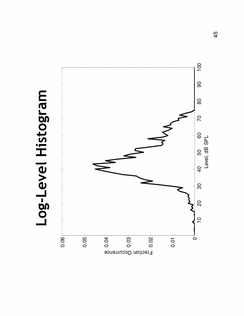
Log-Level Histogram

10

20

30

40

50

60

70

80

90

100

0

0.0

1

0.0

2

0.0

3

0.0

4

0.0

5

0.0

6

Leve

l, d

B S

PL

Fraction Occurrence

46

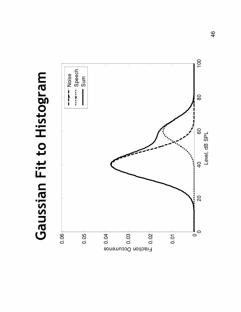
Gaussian Fit to Histogram

02

04

06

08

01

00

0

0.0

1

0.0

2

0.0

3

0.0

4

0.0

5

0.0

6

Leve

l, d

B S

PL

Fraction Occurrence

Nois

e

Spe

ech

Sum

47

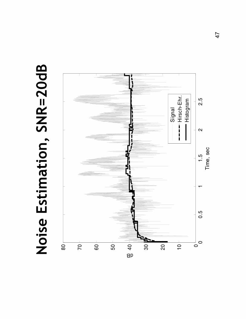
Noise Estimation, SNR=20dB

00

.51

1.5

22

.50

10

20

30

40

50

60

70

80

Tim

e,

sec

dB

Sig

na

l

Hir

sc

h-E

hr.

His

tog

ram

48

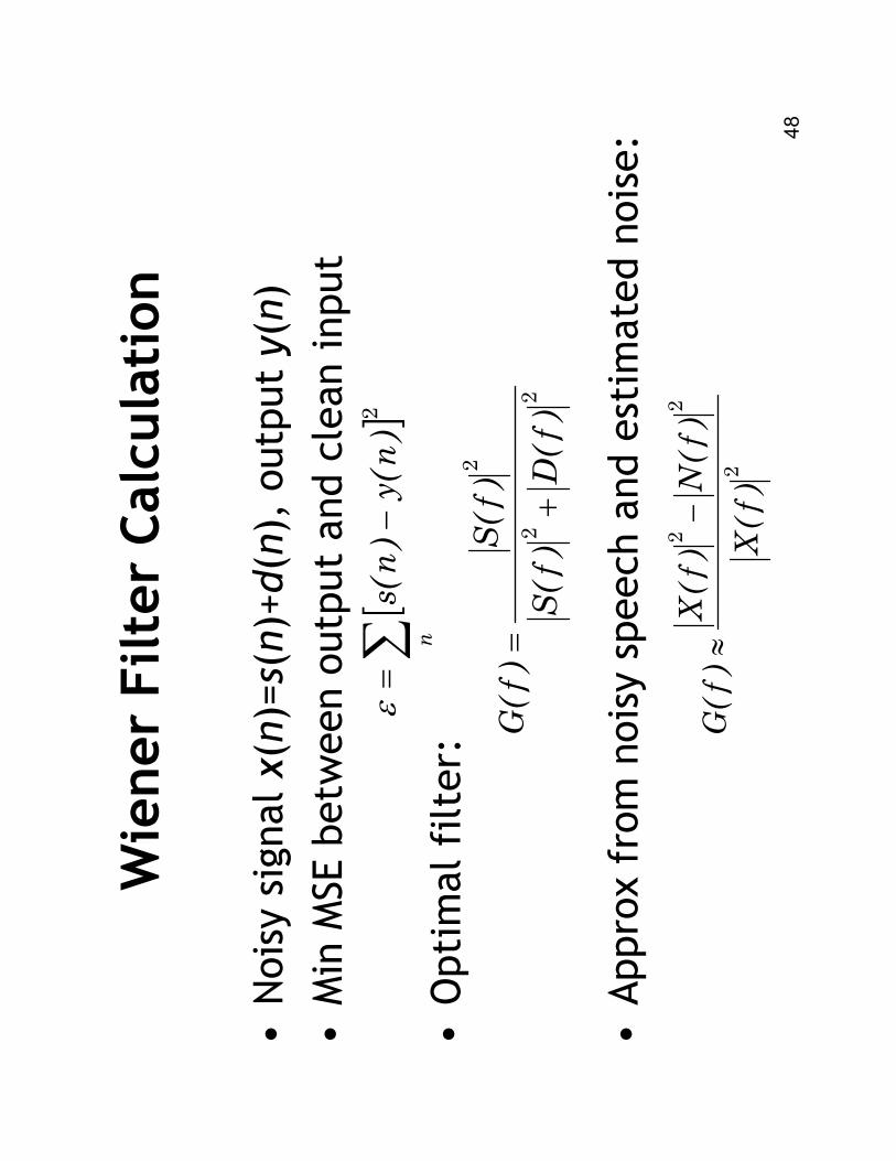
Wiener Filter Calculation

•Noisy signal x(n)=s(n)+d(n), output y(n)

•Min MSE between output and clean input

•Optimal filter:

•Approx from noisy speech and estimated noise:

[]

∑−

=n

)n(y

)n(s

2ε

22

2

)f(

D)f(S

)f(S

)f(

G+

=

2

22

)f(

X

)f(

N)f(

X)f(

G−

≈

49

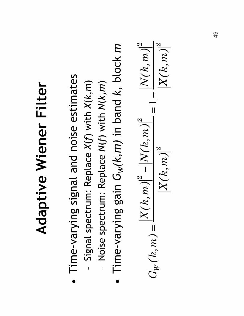
Adaptive W

iener Filter

•Time-varying signal and noise estimates

–Signal spectrum: Replace X(f) with X(k,m

)

–Noise spectrum: Replace N(f) with N(k,m

)

•Time-varying gain G

W(k,m

) in band k, block m

22

2

22

1)

m,k(

X

)m,

k(

N

)m,

k(

X

)m,

k(

N)

m,k(

X)

m,k(

GW

−=

−=

50

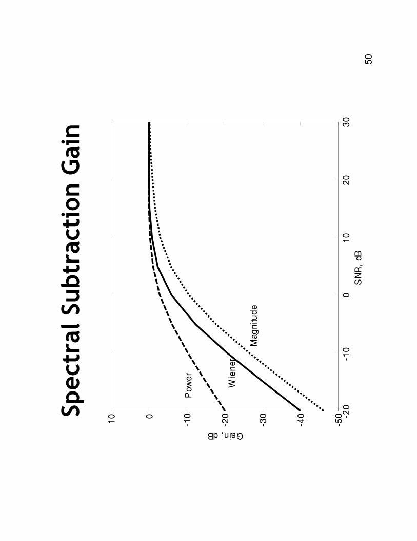
Spectral Subtraction Gain

-20

-10

01

02

03

0-5

0

-40

-30

-20

-100

10

SN

R,

dB

Gain, dB

Pow

er

Wie

ner

Mag

nitu

de

51

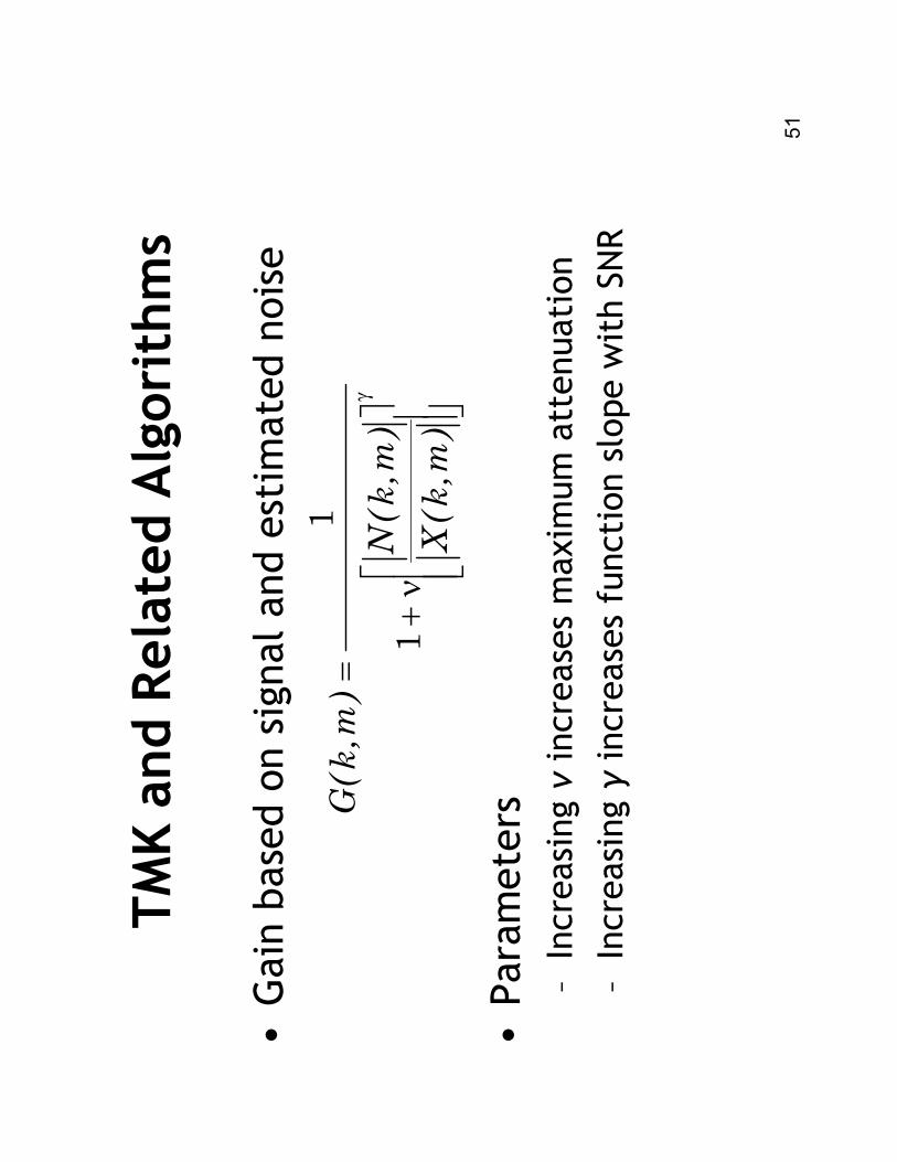
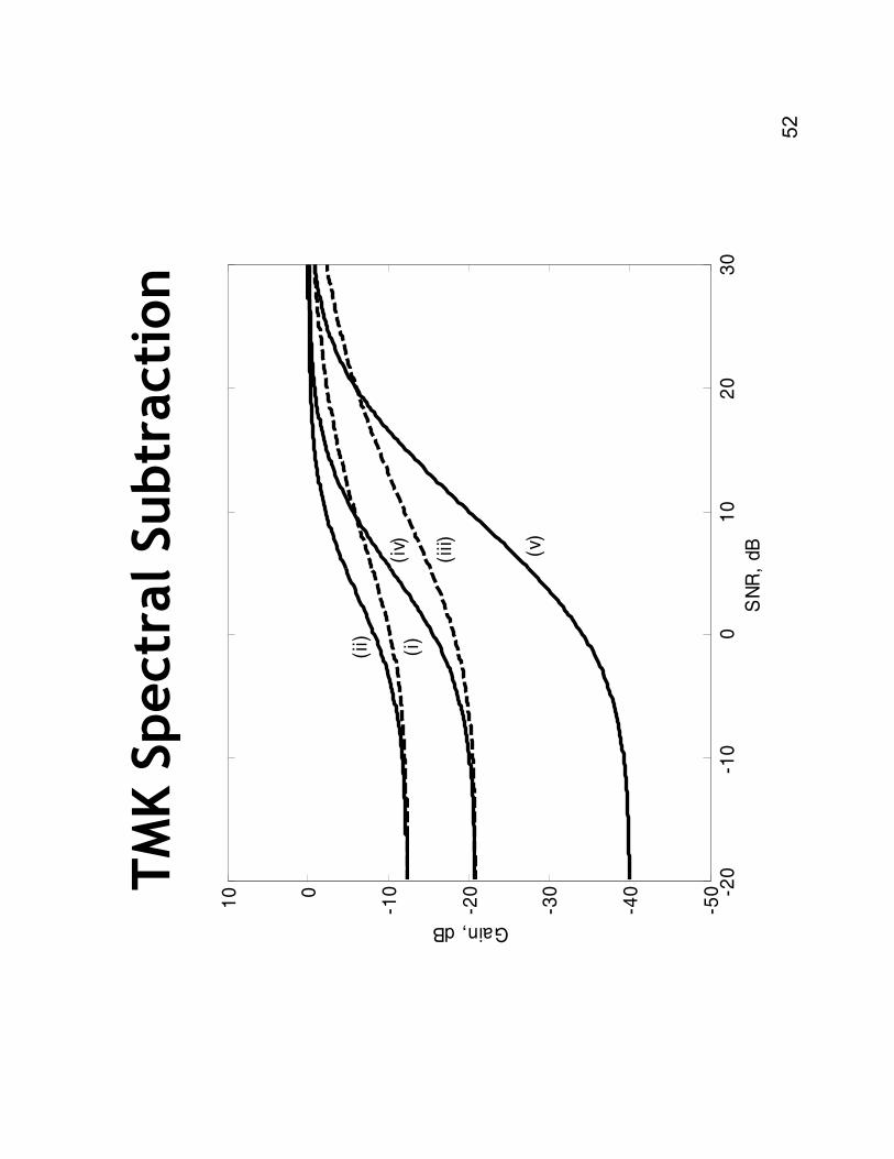
TMK and Related Algorithms

•Gain based on signal and estimated noise

•Parameters

–Increasing νincreases maximum attenuation

–Increasing γincreases function slope with SNR

γ

ν+

=

)m,

k(

X

)m,

k(

N)

m,k(

G

1

1

52

TMK Spectral Subtraction

-20

-10

01

02

03

0-5

0

-40

-30

-20

-100

10

SN

R,

dB

Gain, dB

(i)

(ii)

(iii)

(iv) (v)

53

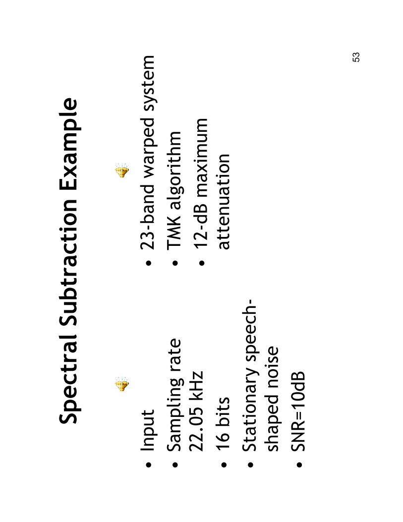
Spectral Subtraction Example

•Input

•Sampling rate

22.05 kHz

•16 bits

•Stationary speech-

shaped noise

•SNR=10dB

•23-band warped system

•TMK algorithm

•12-dB maximum

attenuation

54

Noise Suppression Conclusions

•Little improvement in intelligibility

–Depends on algorithm

–TMK and Ephraim-Malahmost effective

•Some improvement in quality

–TMK shows benefit for NH and HI listeners

–Strongest effect in range of 10 to 20 dB SNR

•Greatest benefit in stationary noise

Feedback Cancellation

56

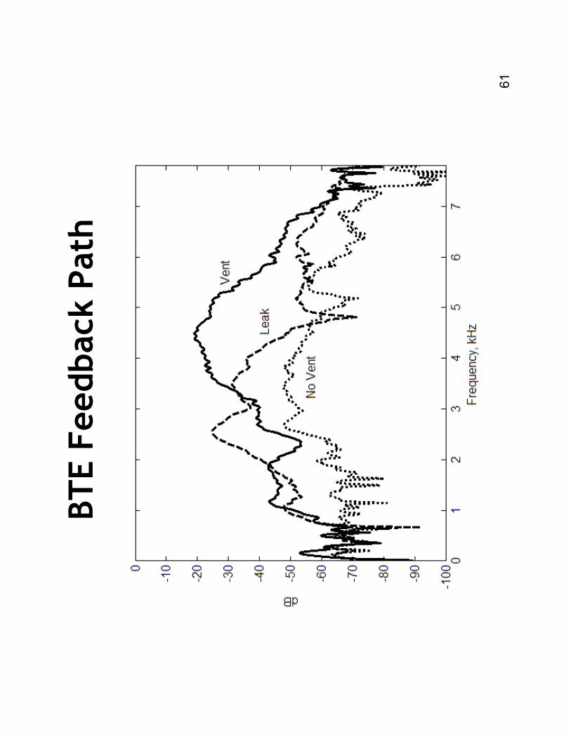
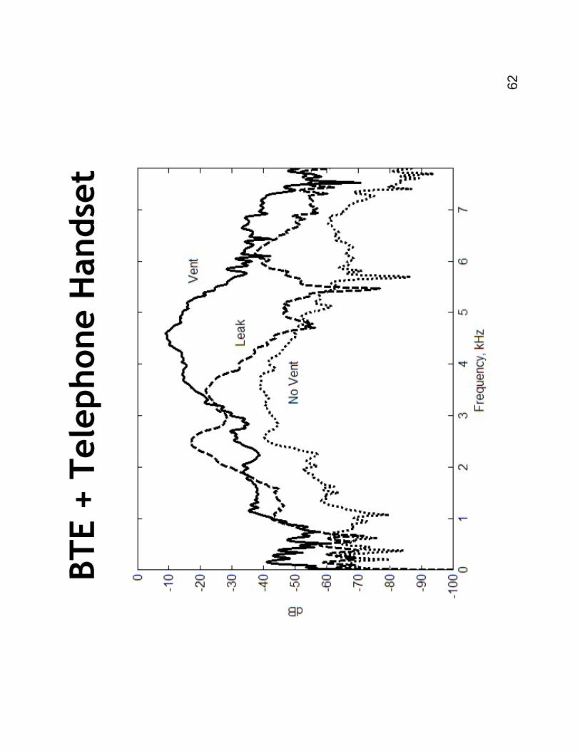
The Problem of Feedback

•Primary sources of feedback

–Acoustic from vent and leaks

–Mechanical from receiver vibration

•Effect on hearing aid

–Instability causes "whistle" or high-frequency tone

–Ringing after sound stops

–Hearing aid amplifier saturates => distortion

•Maximum stable gain

–Maximum gain for operation without whistles

–Problem most acute at high frequencies

57

Algorithm Goals

•Increased gain

–Achieve fitting targets

–Improved speech intelligibility

•No processing artifacts

–Hearing aid always stable

–No whistles due to feedback

–No chirps, momentary tones, or audible gain changes

•Computationally efficient

58

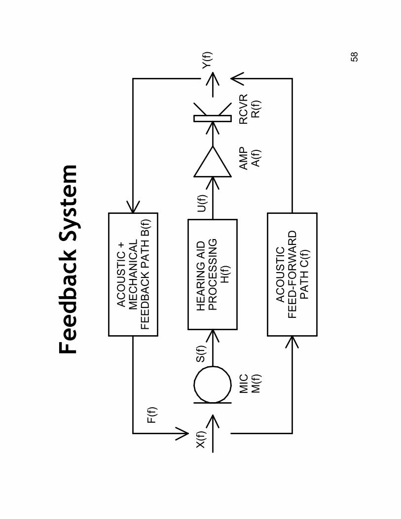
Feedback System

HE

AR

ING

AID

P

RO

CES

SIN

GH

(f)

X(f)

Y(f)

MIC

M(f)

AM

PA

(f)

RC

VR

R(f)

AC

OU

STIC

FE

ED

-FO

RW

AR

DP

ATH

C(f)

AC

OU

STIC

+M

EC

HA

NIC

AL

FE

ED

BA

CK

PA

TH

B(f)

F(f)

U(f)

S(f)

59

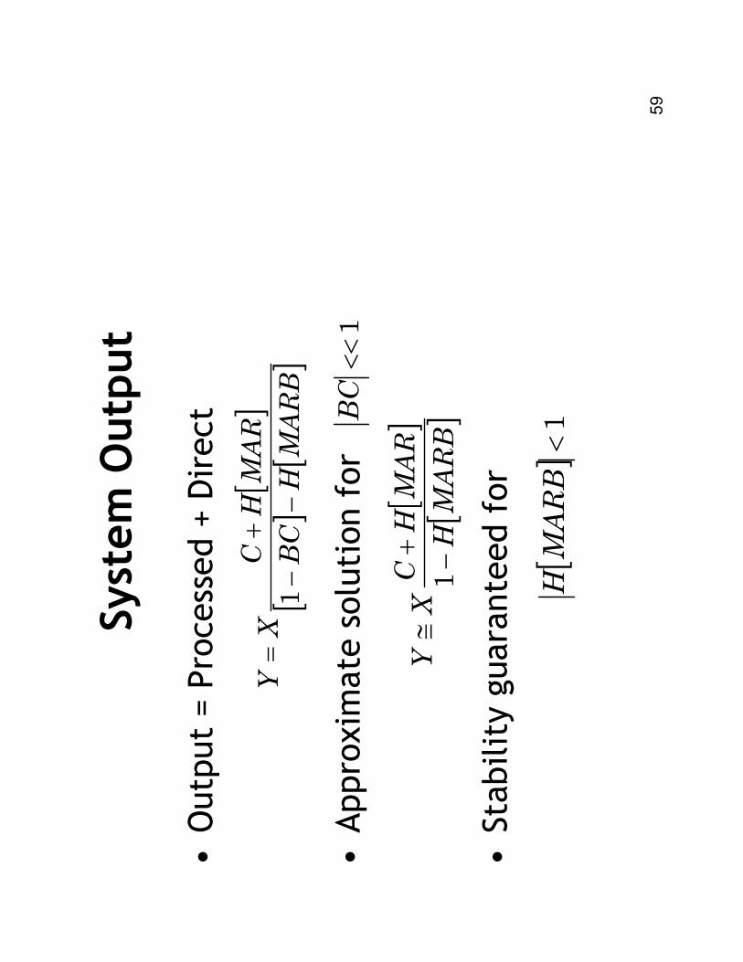
System Output

•Output = Processed + Direct

•Approximate solution for

•Stability guaranteed for[

][

][

]MARB

HBC

MAR

HC

XY

−−

+=

1

1<<

BC

[]

[]

MARB

H

MAR

HC

XY

−+≅

1

[]1

<MARB

H

60

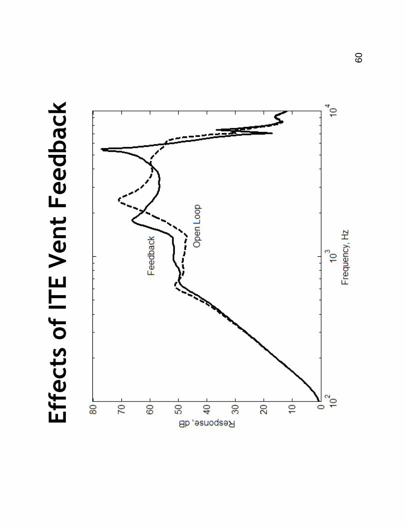
Effects of ITE Vent Feedback

61

BTE Feedback Path

62

BTE + Telephone Handset

63

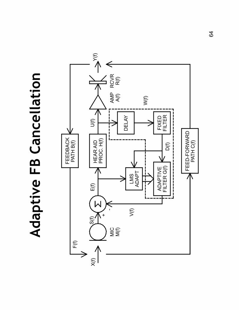
Adaptive Feedback Cancellation

•Model feedback path

–Adaptive model to minimize system power

–Subtract model output from microphone signal

•Why adaptive?

–Feedback path can change over time

–Track changes

•Limitations

–Resolution of the feedback path model

–Ability to track rapid changes

–Cancellation of tonal inputs

–Room reverberation

64

Adaptive FB Cancellation

FE

ED

BA

CK

PATH

B(f)

HE

AR

AID

P

RO

C. H

(f)

DE

LAY

LM

SA

DA

PT

FIX

ED

FIL

TE

RA

DA

PTIV

EFIL

TE

R G

(f)

+-

D(f)

X(f)

Y(f)

E(f)

S(f) V

(f)

MIC

M(f)

AM

PA

(f)

RC

VR

R(f)

U(f)

FE

ED

-FO

RW

AR

DPATH

C(f)

F(f)

W(f)

65

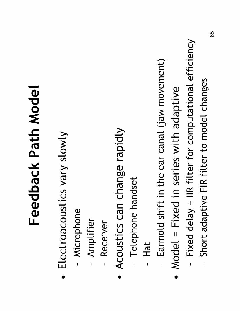
Feedback Path Model

•Electroacousticsvary slowly

–Microphone

–Amplifier

–Receiver

•Acoustics can change rapidly

–Telephone handset

–Hat

–Earm

oldshift in the ear canal (jaw movement)

•Model = Fixed in series with adaptive

–Fixed delay + IIR filter for computational efficiency

–Short adaptive FIR filter to model changes

66

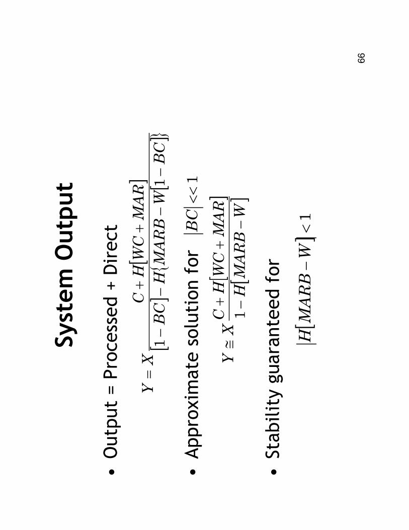
System Output

•Output = Processed + Direct

•Approximate solution for

•Stability guaranteed for[

][

][

]{

}BC

WMARB

HBC

MAR

WC

HC

XY

−−

−−

++

=1

1

1<<

BC

[]1

<−W

MARB

H

[]

[]

WMARB

H

MAR

WC

HC

XY

−−

++

≅1

67

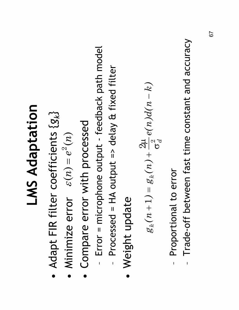
LMS Adaptation

•Adapt FIR filter coefficients {gk}

•Minimize error

•Compare error with processed

–Error = microphone output -feedback path model

–Processed = HA output => delay & fixed filter

•Weight update

–Proportional to error

–Trade-off between fast time constant and accuracy

)(

)(

2n

en

=ε

)k

n(d)

n(e

)n(

g)

n(

gd

kk

−σµ

+=

+2

21

68

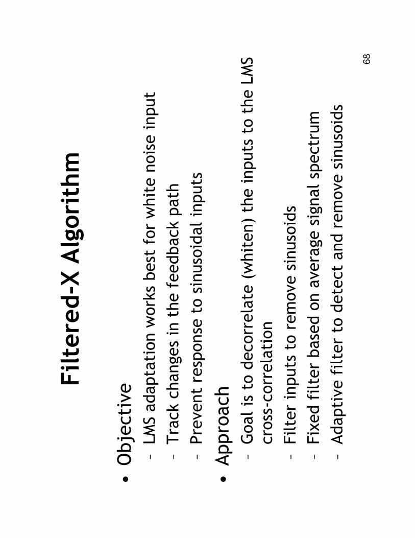
Filtered-X Algorithm

•Objective

–LMS adaptation works best for white noise input

–Track changes in the feedback path

–Prevent response to sinusoidal inputs

•Approach

–Goal is to decorrelate

(whiten) the inputs to the LMS

cross-correlation

–Filter inputs to remove sinusoids

–Fixed filter based on average signal spectrum

–Adaptive filter to detect and remove sinusoids

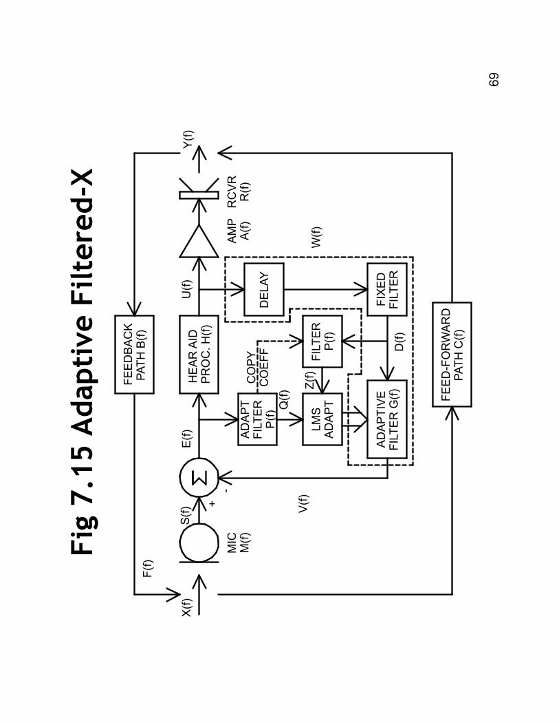
69

Fig 7.15 Adaptive Filtered-X

FE

ED

BA

CK

PATH

B(f)

HE

AR

AID

P

RO

C. H

(f)

DE

LAY

AD

APT

FIL

TE

RP

(f)

FIL

TER

P(f)

LM

SA

DA

PT

FIX

ED

FIL

TER

AD

AP

TIV

EFIL

TER

G(f)

+-

D(f)

X(f)

Y(f)

E(f)

S(f) V(f)

MIC

M(f)

AM

PA

(f)

RC

VR

R(f)

Q(f) Z

(f)

U(f)

FE

ED

-FO

RW

AR

DPATH

C(f)

F(f)

CO

PY

CO

EFF

W(f)

70

Feedback Conclusions

•Feedback cancellation

–Model the feedback path

–Subtract model output from microphone signal

–LMS adaptive filter update

–Filtered-X approach most effective

•Processing effectiveness

–Generally get 10 -15 dB headroom increase

–Increased gain gives increased audibility

–Increased stability improves sound quality

•Problems remain

–LMS tries to cancel tones and narrowband inputs

–Reverberation

–Clients don't like initialization probe signal

–Linear model affected by distortion (e.g. power aids)

Microphones and Arrays

72

Omnidirectional Microphone

•Single Surface

–Measure pressure at a point in space

–Proportional to membrane displacement

•Microphone Technology

–Moving coil

–Electret

–Silicon

73

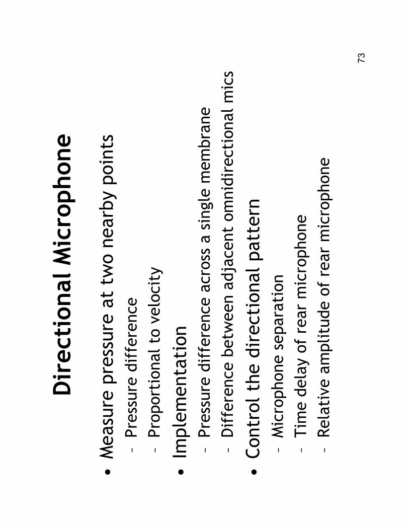
Directional Microphone

•Measure pressure at two nearby points

–Pressure difference

–Proportional to velocity

•Implementation

–Pressure difference across a single membrane

–Difference between adjacent omnidirectional mics

•Control the directional pattern

–Microphone separation

–Time delay of rear microphone

–Relative amplitude of rear microphone

74

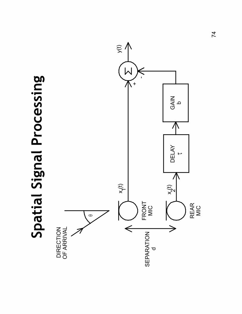
Spatial Signal Processing

DELAY

FR

ON

TM

IC

RE

AR

MIC

SE

PA

RATIO

Nd

+-

x (t)

x (t)

y(t)

1 2

θ

DIR

EC

TIO

NO

F A

RR

IVA

L

τG

AIN

b

75

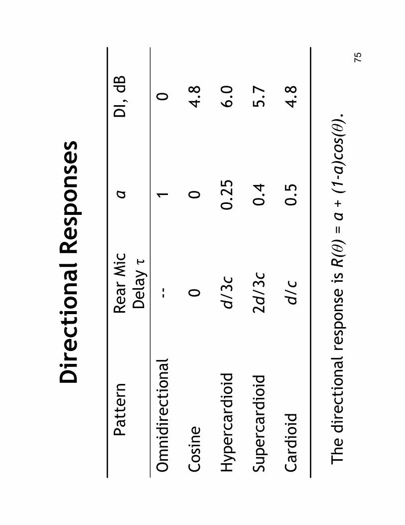
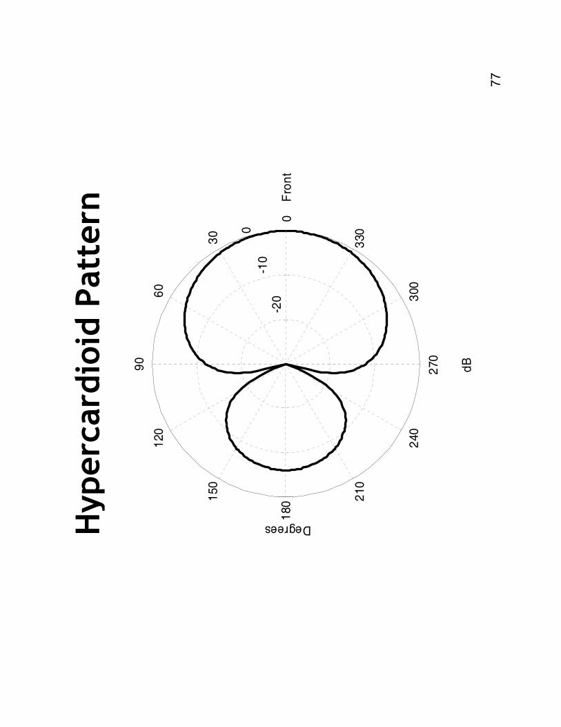
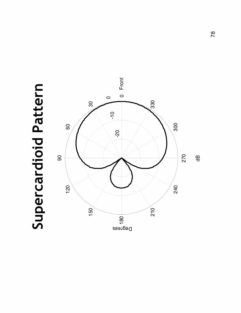
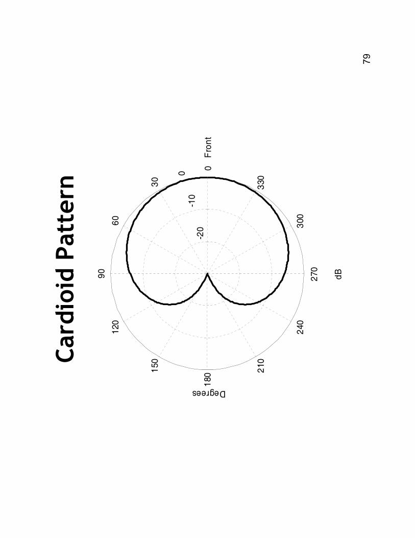
Directional Responses

The directional response is R(θ) = a + (1-a)cos(θ).

4.8

0.5

d/c

Cardioid

5.7

0.4

2d/3c

Supercardioid

6.0

0.25

d/3c

Hypercardioid

4.8

00

Cosine

01

--Omnidirectional

DI, dB

aRear Mic

Delay τ

Pattern

76

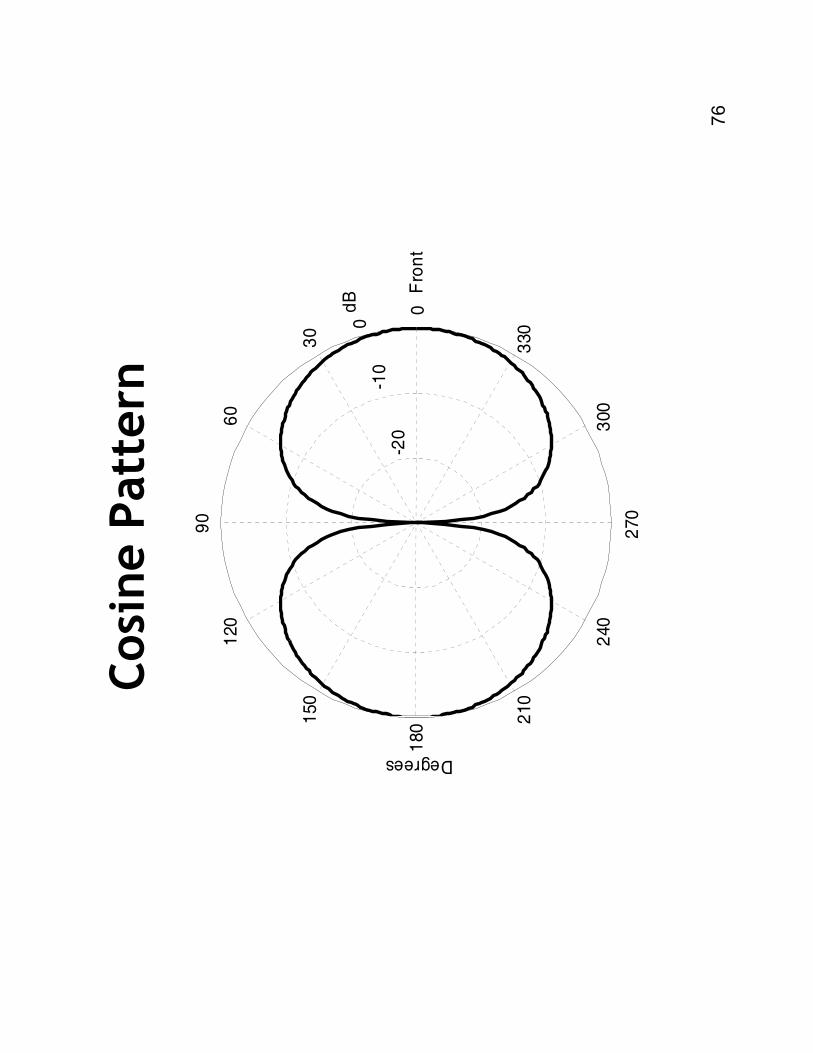
Cosine Pattern

-2

0

-10

0

30

210

60

240

90

270

120

300

150

330

180

0

Degrees

Fro

nt

dB

77

Hypercardioid

Pattern

-2

0

-10

0

30

210

60

240

90

270

120

300

150

330

180

0

dB

Degrees

Fro

nt

78

Supercardioid

Pattern

-2

0

-10

0

30

210

60

240

90

270

120

300

150

330

180

0

dB

Degrees

Fro

nt

79

Cardioid

Pattern

-2

0

-10

0

30

210

60

240

90

270

120

300

150

330

180

0

dB

Degrees

Fro

nt

80

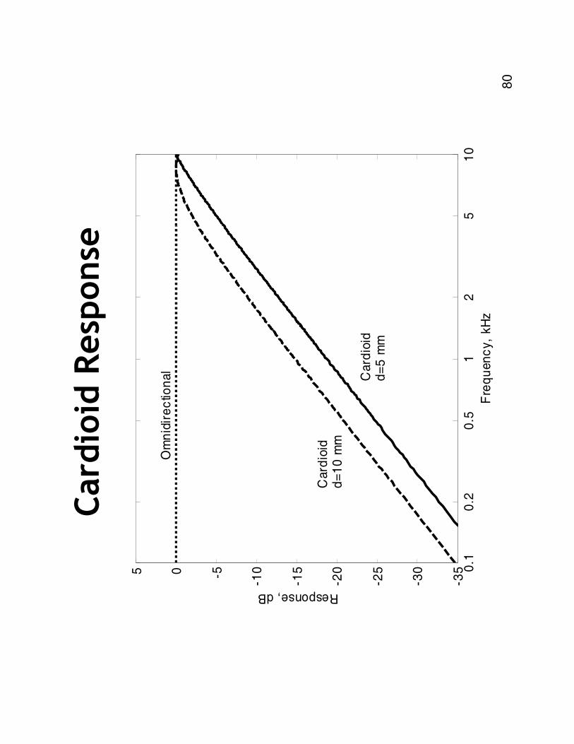
Cardioid

Response

0.1

0.2

0.5

12

51

0-3

5

-30

-25

-20

-15

-10-505

Fre

qu

en

cy,

kH

z

Response, dB

Om

nid

ire

ctio

nal

Card

ioid

d=

10

mm

Card

ioid

d=

5 m

m

81

Adaptive Microphone Arrays

•Start with 2 microphones

–Extension of directional microphone technology

–Can be built into hearing-aid case

•Multi-microphone arrays

–Combine outputs from multiple microphones

–Improved directivity (DI) compared to 2-mic array

–Fixed combination of outputs

–Adaptive combination of outputs

82

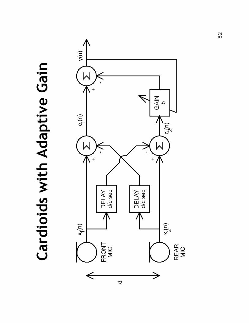
Cardioids with Adaptive Gain

FR

ON

TM

IC

REA

RM

IC

GA

INb

x (n)

x (n)

1 2

+-

y(n

)

+- -

+

DE

LAY

d/c

sec

DE

LAY

d/c

sec

c (n)

1

c (n)

2

d

83

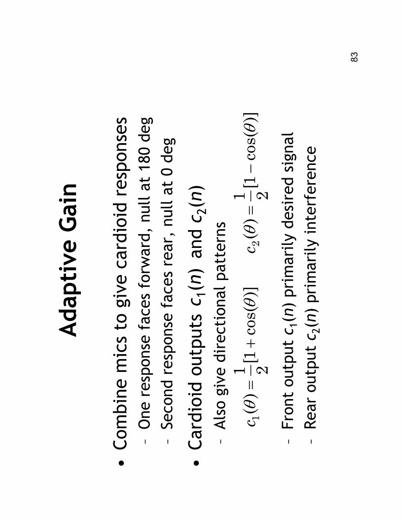
Adaptive Gain

•Combine micsto give cardioidresponses

–One response faces forward, null at 180 deg

–Second response faces rear, null at 0 deg

•Cardioidoutputs and c2(n)

–Also give directional patterns

–Front output c 1(n) primarily desired signal

–Rear output c 2(n) primarily interference

c 1(n)

)]cos(

1[21

)(1

θθ

+=

c)]

cos(

1[21

)(2

θθ

−=

c

84

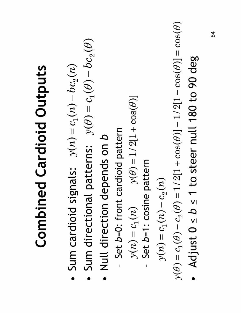
Combined Cardioid

Outputs

•Sum cardioidsignals:

•Sum directional patterns:

•Null direction depends on b

–Set b=0: front cardioidpattern

–Set b=1: cosine pattern

•Adjust 0 ≤

b≤1 to steer null 180 to 90 deg

)(

)(

)(

21

nbc

nc

ny

−=

)(

)(

1n

cn

y=

)(

)(

)(

21

nc

nc

ny

−=

)(

)(

)(

21

θθ

θbc

cy

−=

)]cos(

1[2/

1)

(θ

θ+

=y

)cos(

)]cos(

1[2/

1)]

cos(

1[2/

1)

()

()

(2

1θ

θθ

θθ

θ=

−−

+=

−=

cc

y

85

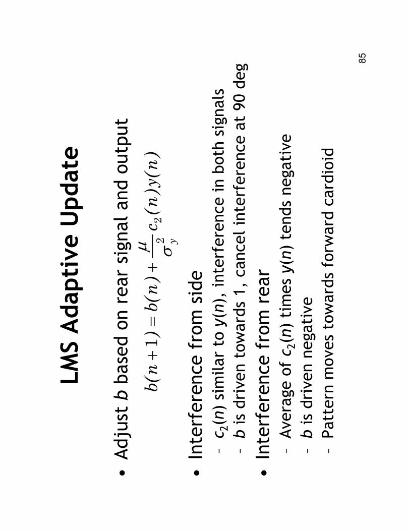
LMS Adaptive Update

•Adjust bbased on rear signal and output

•Interference from side

–c 2(n) similar to y(n), interference in both signals

–bis driven towards 1, cancel interference at 90 deg

•Interference from rear

–Average ofc 2(n) times y(n) tends negative

–bis driven negative

–Pattern moves towards forward cardioid)n(y)

n(

c)n(b

)n(b

y

22

1σµ

+=

+

86

Microphone Conclusions

•Summary from Walden et al(2003):

–Directional micstest better than real-world results

–Environment often limits directional benefit

–Benefit should be expected only when the signal

source is in front of and relatively near the listener

and the interference is spatially separated

–Omnidirectional mode should be the default

AdditionalProcessing

Areas

88

Additional Areas, I

•Electro-acoustic interactions

–Head and external ear modify microphone input

–Vent reduces system low-frequency response

–Occlusion effect: own voice louder

•Wind noise

–Wind flow over microphone generates turbulence

–Directional micsespecially sensitive

•Spectral enhancement

–Broader auditory filters reduce spectral contrast

–Modify short-time spectrum to increase contrast

89

Additional Areas, II

•Sound classification

–Change parameters for different environments

–Identify environments to set optimum processing

•Binaural processing

–Link the hearing aids at the two ears

–Low-power short-range communication link

–Synchronize device parameter settings

–Compare signals for compression and noise

suppression

Conclusions

91

Conclusions

•Hearing aid = perceptual engineering

–Designs apply criteria such as MMSE or Max Likelihood

–These criteria ignore perception

–Need to consider the human listener as well

•Problems remain

–Have not solved the basic problem of speech

intelligibility in noise

–Most algorithms are not effective despite having a

strong intuitive appeal

92

•April 2008

•Plu

ral

Publis

hin

g,

San D

iego