1 / 16

Digital Communications III (ECE 154C)

Introduction to Coding and Information Theory

Tara Javidi

These lecture notes were originally developed by late Prof. J. K. Wolf.

UC San Diego

Spring 2014

Source Coding: Lossless

Compression

Source Coding

• Source Coding

• Basic Definitions

Larger Alphabet

Huffman Codes

Class Work

2 / 16

Source Coding: A Simple Example

Source Coding

• Source Coding

• Basic Definitions

Larger Alphabet

Huffman Codes

Class Work

3 / 16

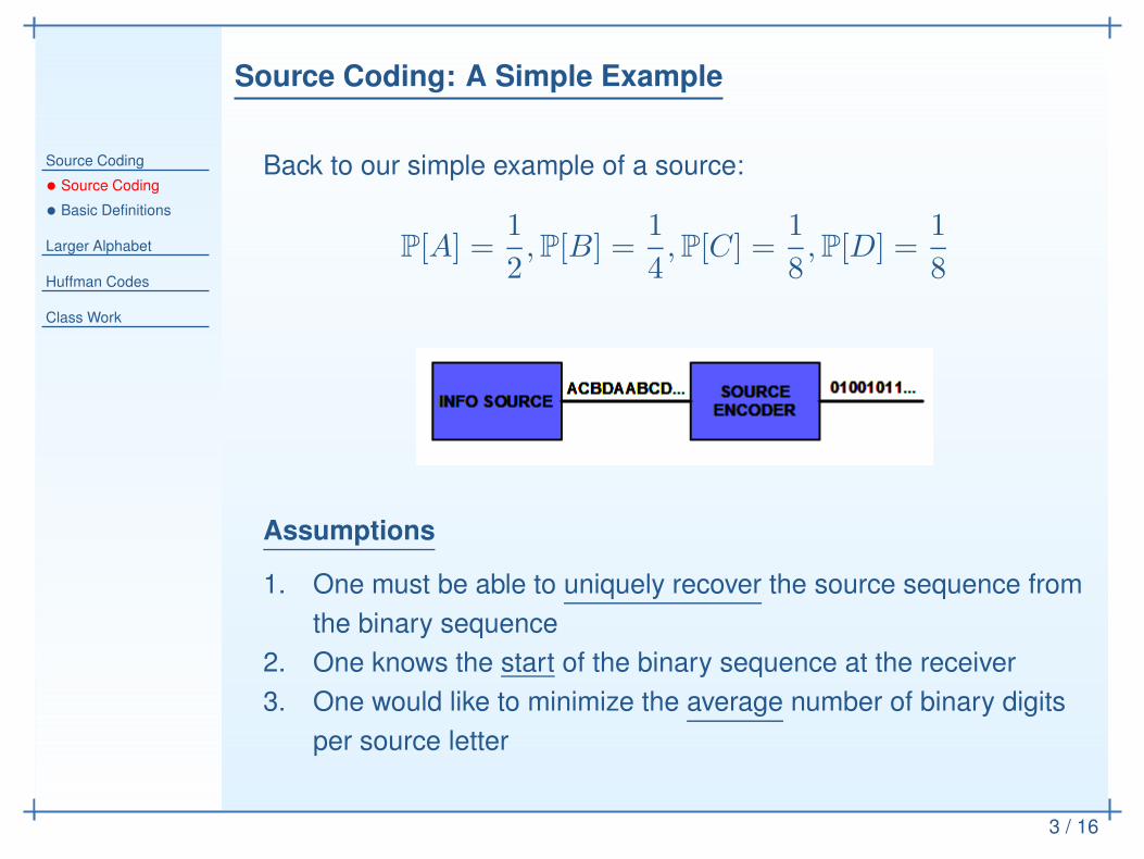
Back to our simple example of a source:

P[A] =1

2,P[B] =

1

4,P[C] =

1

8,P[D] =

1

8

Assumptions

1. One must be able to uniquely recover the source sequence from

the binary sequence

2. One knows the start of the binary sequence at the receiver

3. One would like to minimize the average number of binary digits

per source letter

Source Coding: A Simple Example

Source Coding

• Source Coding

• Basic Definitions

Larger Alphabet

Huffman Codes

Class Work

3 / 16

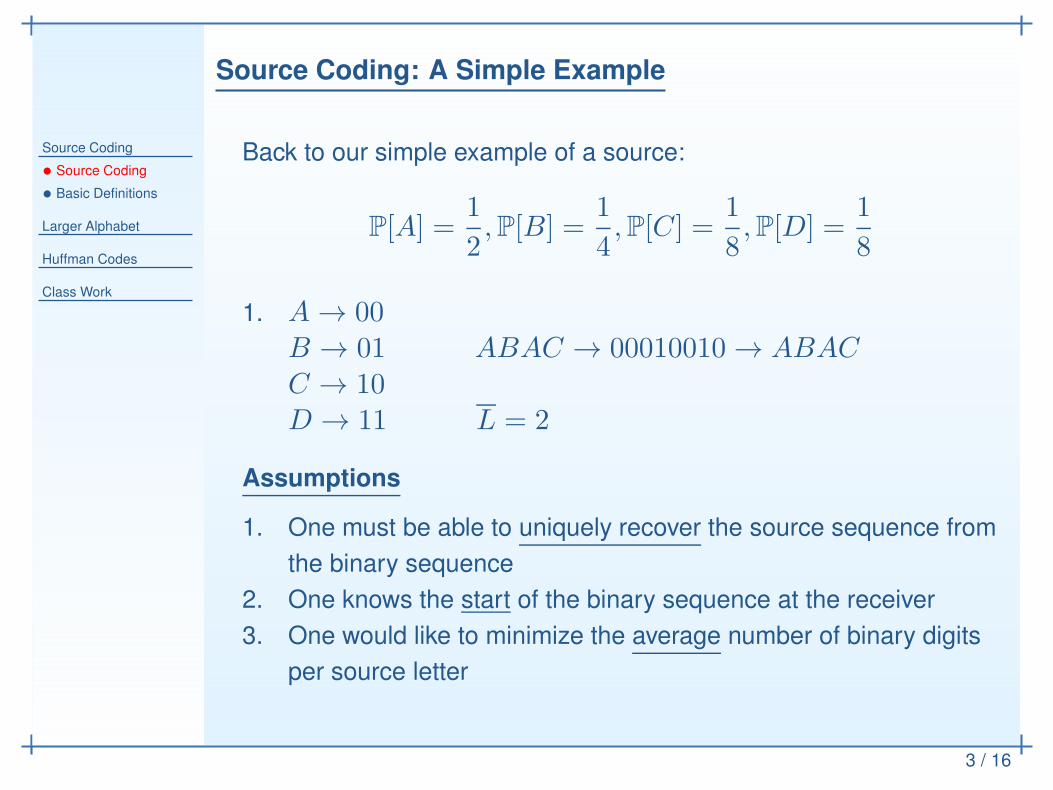
Back to our simple example of a source:

P[A] =1

2,P[B] =

1

4,P[C] =

1

8,P[D] =

1

8

1. A → 00B → 01 ABAC → 00010010 → ABAC

C → 10D → 11 L = 2

Assumptions

1. One must be able to uniquely recover the source sequence from

the binary sequence

2. One knows the start of the binary sequence at the receiver

3. One would like to minimize the average number of binary digits

per source letter

Source Coding: A Simple Example

Source Coding

• Source Coding

• Basic Definitions

Larger Alphabet

Huffman Codes

Class Work

3 / 16

Back to our simple example of a source:

P[A] =1

2,P[B] =

1

4,P[C] =

1

8,P[D] =

1

8

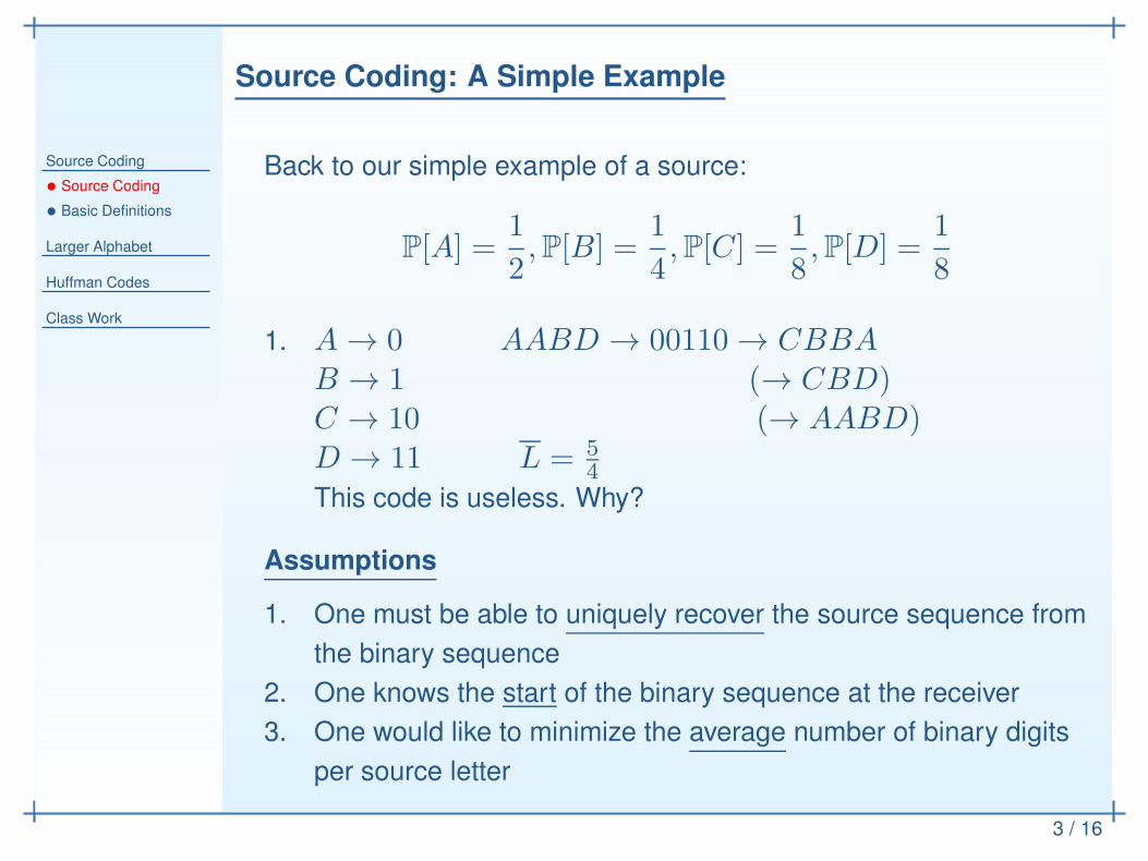
1. A → 0 AABD → 00110 → CBBA

B → 1 (→ CBD)C → 10 (→ AABD)D → 11 L = 5

4

This code is useless. Why?

Assumptions

1. One must be able to uniquely recover the source sequence from

the binary sequence

2. One knows the start of the binary sequence at the receiver

3. One would like to minimize the average number of binary digits

per source letter

Source Coding: A Simple Example

Source Coding

• Source Coding

• Basic Definitions

Larger Alphabet

Huffman Codes

Class Work

3 / 16

Back to our simple example of a source:

P[A] =1

2,P[B] =

1

4,P[C] =

1

8,P[D] =

1

8

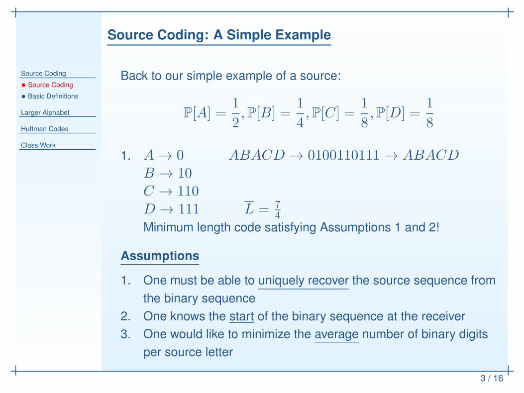
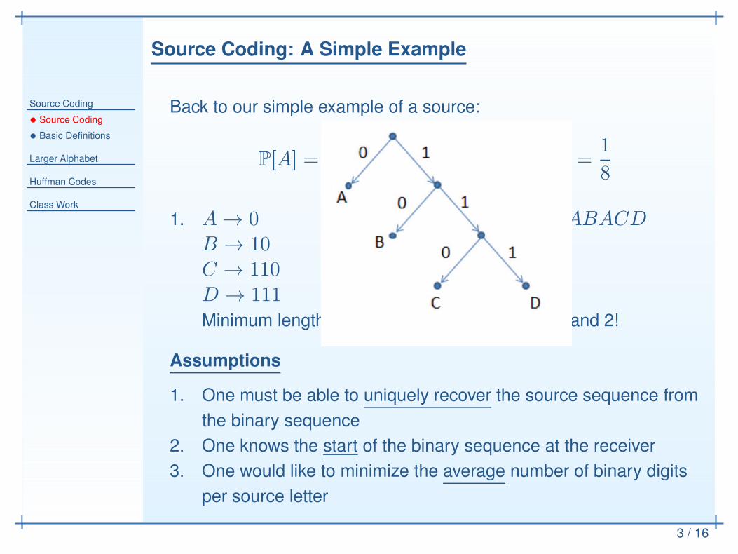
1. A → 0 ABACD → 0100110111 → ABACD

B → 10C → 110D → 111 L = 7

4

Minimum length code satisfying Assumptions 1 and 2!

Assumptions

1. One must be able to uniquely recover the source sequence from

the binary sequence

2. One knows the start of the binary sequence at the receiver

3. One would like to minimize the average number of binary digits

per source letter

Source Coding: A Simple Example

Source Coding

• Source Coding

• Basic Definitions

Larger Alphabet

Huffman Codes

Class Work

3 / 16

Back to our simple example of a source:

P[A] =1

2,P[B] =

1

4,P[C] =

1

8,P[D] =

1

8

1. A → 0 ABACD → 0100110111 → ABACD

B → 10C → 110D → 111 L = 7

4

Minimum length code satisfying Assumptions 1 and 2!

Assumptions

1. One must be able to uniquely recover the source sequence from

the binary sequence

2. One knows the start of the binary sequence at the receiver

3. One would like to minimize the average number of binary digits

per source letter

Source Coding: Basic Definitions

Source Coding

• Source Coding

• Basic Definitions

Larger Alphabet

Huffman Codes

Class Work

4 / 16

Codeword (aka Block Code)

Each source symbol is represented by some sequence of coded

symbols called a code word

Non-Singular Code

Code words are distinct

Uniquely Decodable (U.D.) Code

Every distinct concatenation of m code words is distinct for every

finite m

Instantaneous Code

A U.D. Code where we can decode each code word without seeing

subsequent code words

Source Coding: Basic Definitions

Source Coding

• Source Coding

• Basic Definitions

Larger Alphabet

Huffman Codes

Class Work

4 / 16

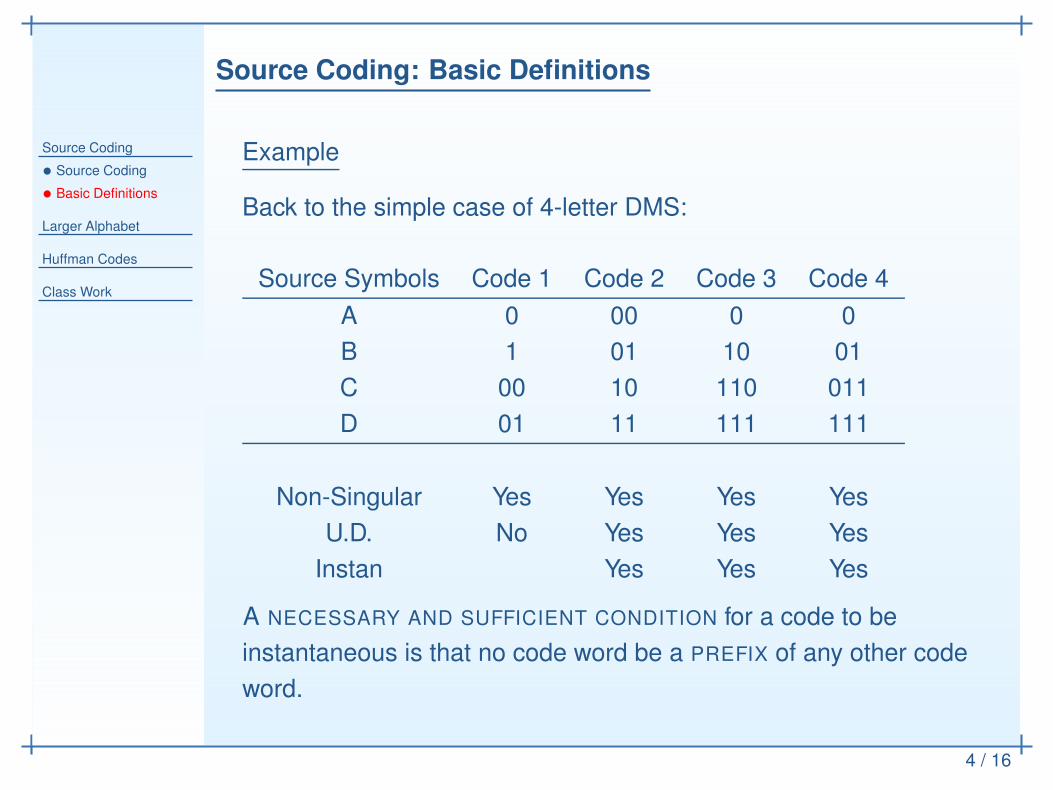
Example

Back to the simple case of 4-letter DMS:

Source Symbols Code 1 Code 2 Code 3 Code 4

A 0 00 0 0

B 1 01 10 01

C 00 10 110 011

D 01 11 111 111

Non-Singular Yes Yes Yes Yes

U.D. No Yes Yes Yes

Instan Yes Yes Yes

A NECESSARY AND SUFFICIENT CONDITION for a code to be

instantaneous is that no code word be a PREFIX of any other code

word.

Coding Several Source Symbol at

a Time

Source Coding

Larger Alphabet

• Example 1

Huffman Codes

Class Work

5 / 16

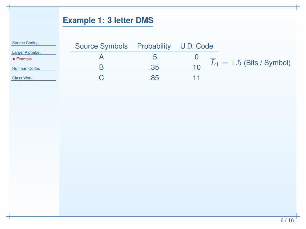
Example 1: 3 letter DMS

Source Coding

Larger Alphabet

• Example 1

Huffman Codes

Class Work

6 / 16

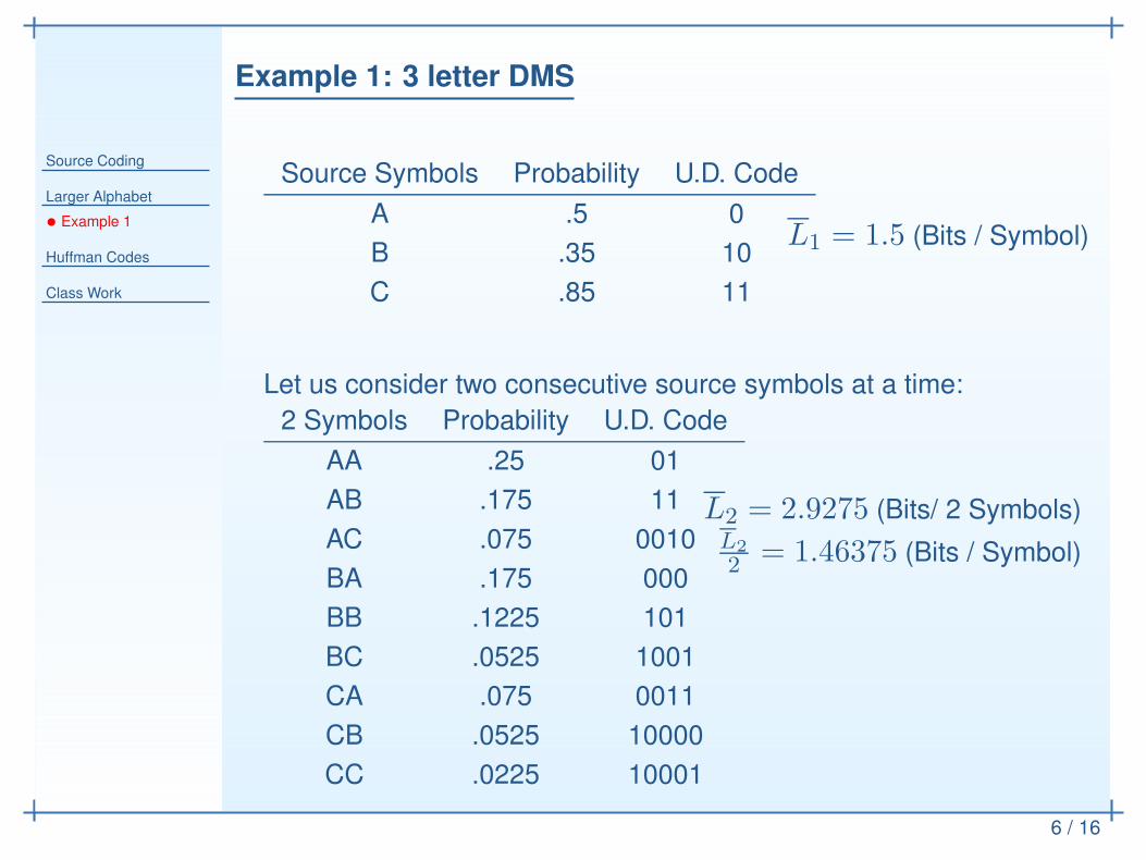
Source Symbols Probability U.D. Code

A .5 0

B .35 10

C .85 11

L1 = 1.5 (Bits / Symbol)

Example 1: 3 letter DMS

Source Coding

Larger Alphabet

• Example 1

Huffman Codes

Class Work

6 / 16

Source Symbols Probability U.D. Code

A .5 0

B .35 10

C .85 11

L1 = 1.5 (Bits / Symbol)

Let us consider two consecutive source symbols at a time:

2 Symbols Probability U.D. Code

AA .25 01

AB .175 11

AC .075 0010

BA .175 000

BB .1225 101

BC .0525 1001

CA .075 0011

CB .0525 10000

CC .0225 10001

L2 = 2.9275 (Bits/ 2 Symbols)L2

2= 1.46375 (Bits / Symbol)

Example 1: 3 letter DMS

Source Coding

Larger Alphabet

• Example 1

Huffman Codes

Class Work

6 / 16

In other words,

1. It is more efficient to build a code for 2 source symbols!

2. Is it possible to decrease the length more and more by

increasing the alphabet size?

To see the answer to the above question, it is useful if we can say

precisely characterize the best code. The codes given above are

Huffman Codes. The procedure for making Huffman Codes will be

described next.

Minimizing average length

Source Coding

Larger Alphabet

Huffman Codes

• Binary Huffman Code

• Example I

• Example II

• Optimality

• Shannon-Fano Codes

Class Work

7 / 16

Binary Huffman Codes

Source Coding

Larger Alphabet

Huffman Codes

• Binary Huffman Code

• Example I

• Example II

• Optimality

• Shannon-Fano Codes

Class Work

8 / 16

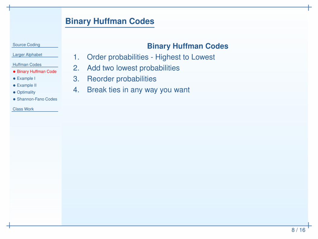
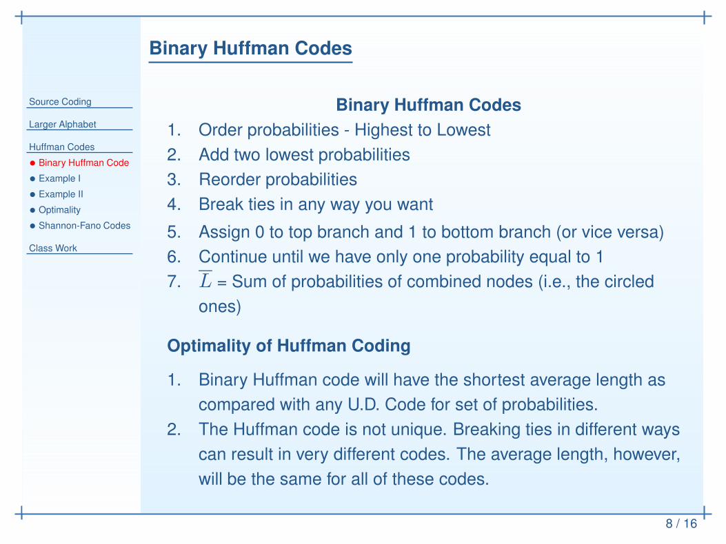
Binary Huffman Codes

1. Order probabilities - Highest to Lowest

2. Add two lowest probabilities

3. Reorder probabilities

4. Break ties in any way you want

Binary Huffman Codes

Source Coding

Larger Alphabet

Huffman Codes

• Binary Huffman Code

• Example I

• Example II

• Optimality

• Shannon-Fano Codes

Class Work

8 / 16

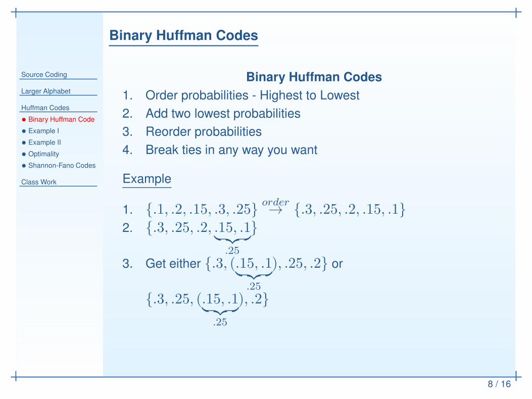
Binary Huffman Codes

1. Order probabilities - Highest to Lowest

2. Add two lowest probabilities

3. Reorder probabilities

4. Break ties in any way you want

Example

1. {.1, .2, .15, .3, .25}order→ {.3, .25, .2, .15, .1}

2. {.3, .25, .2, .15, .1︸ ︷︷ ︸

.25

}

3. Get either {.3, (.15, .1︸ ︷︷ ︸

.25

), .25, .2} or

{.3, .25, (.15, .1︸ ︷︷ ︸

.25

), .2}

Binary Huffman Codes

Source Coding

Larger Alphabet

Huffman Codes

• Binary Huffman Code

• Example I

• Example II

• Optimality

• Shannon-Fano Codes

Class Work

8 / 16

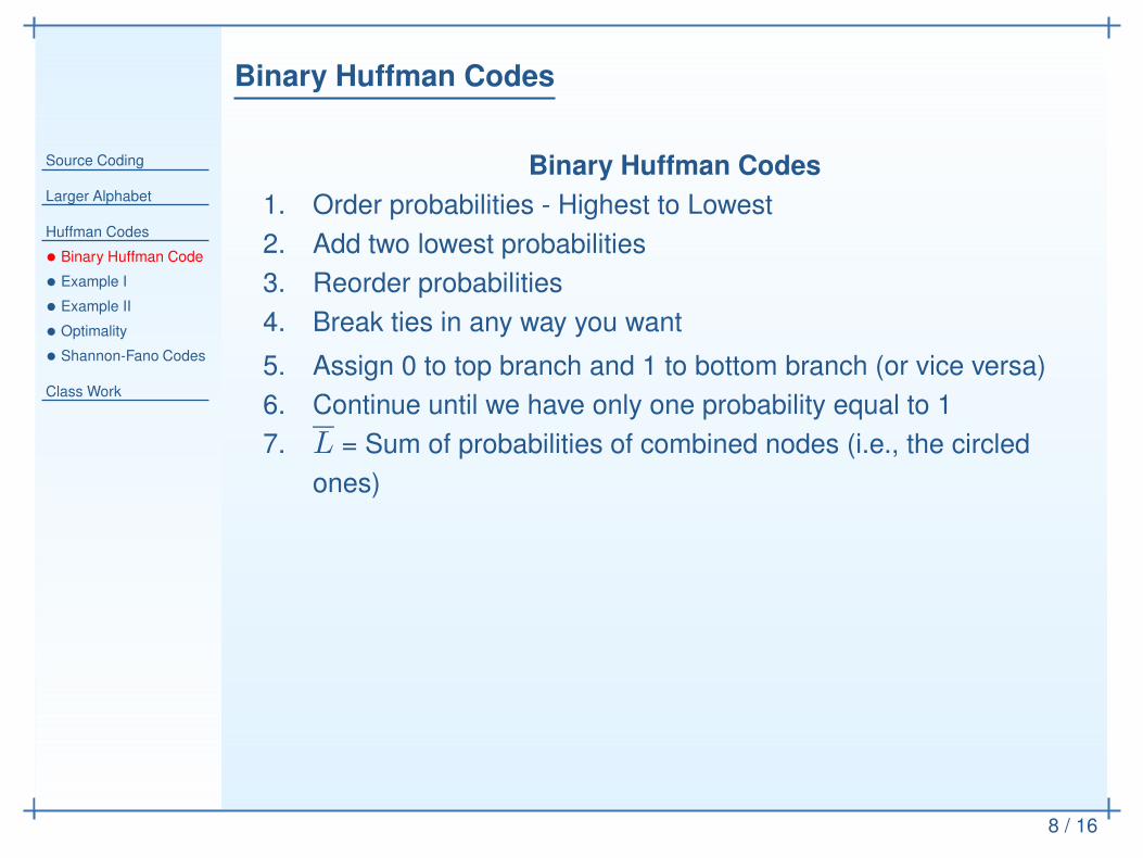
Binary Huffman Codes

1. Order probabilities - Highest to Lowest

2. Add two lowest probabilities

3. Reorder probabilities

4. Break ties in any way you want

5. Assign 0 to top branch and 1 to bottom branch (or vice versa)

6. Continue until we have only one probability equal to 1

7. L = Sum of probabilities of combined nodes (i.e., the circled

ones)

Binary Huffman Codes

Source Coding

Larger Alphabet

Huffman Codes

• Binary Huffman Code

• Example I

• Example II

• Optimality

• Shannon-Fano Codes

Class Work

8 / 16

Binary Huffman Codes

1. Order probabilities - Highest to Lowest

2. Add two lowest probabilities

3. Reorder probabilities

4. Break ties in any way you want

5. Assign 0 to top branch and 1 to bottom branch (or vice versa)

6. Continue until we have only one probability equal to 1

7. L = Sum of probabilities of combined nodes (i.e., the circled

ones)

Optimality of Huffman Coding

1. Binary Huffman code will have the shortest average length as

compared with any U.D. Code for set of probabilities.

2. The Huffman code is not unique. Breaking ties in different ways

can result in very different codes. The average length, however,

will be the same for all of these codes.

Huffman Coding: Example

Source Coding

Larger Alphabet

Huffman Codes

• Binary Huffman Code

• Example I

• Example II

• Optimality

• Shannon-Fano Codes

Class Work

9 / 16

Example Continued

1. {.1, .2, .15, .3, .25}order→ {.3, .25, .2, .15, .1}

Huffman Coding: Example

Source Coding

Larger Alphabet

Huffman Codes

• Binary Huffman Code

• Example I

• Example II

• Optimality

• Shannon-Fano Codes

Class Work

9 / 16

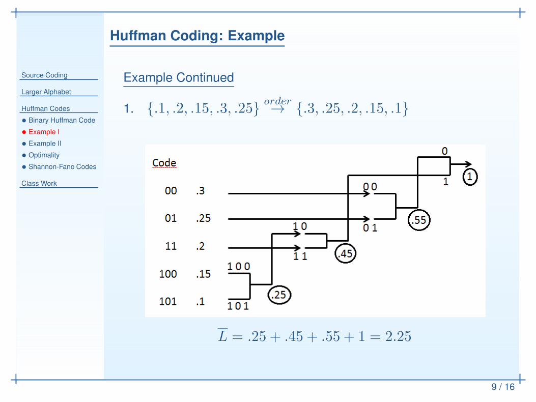
Example Continued

1. {.1, .2, .15, .3, .25}order→ {.3, .25, .2, .15, .1}

L = .25 + .45 + .55 + 1 = 2.25

Huffman Coding: Example

Source Coding

Larger Alphabet

Huffman Codes

• Binary Huffman Code

• Example I

• Example II

• Optimality

• Shannon-Fano Codes

Class Work

9 / 16

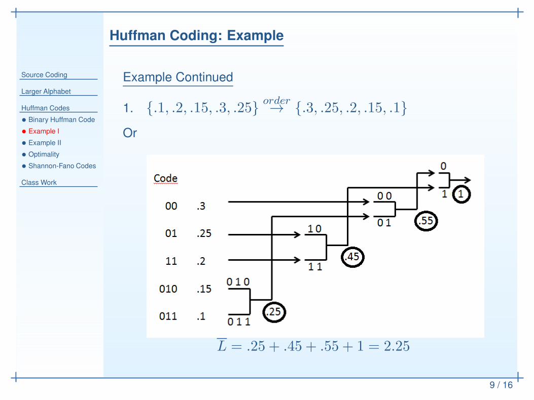
Example Continued

1. {.1, .2, .15, .3, .25}order→ {.3, .25, .2, .15, .1}

Or

L = .25 + .45 + .55 + 1 = 2.25

Huffman Coding: Tie Breaks

Source Coding

Larger Alphabet

Huffman Codes

• Binary Huffman Code

• Example I

• Example II

• Optimality

• Shannon-Fano Codes

Class Work

10 / 16

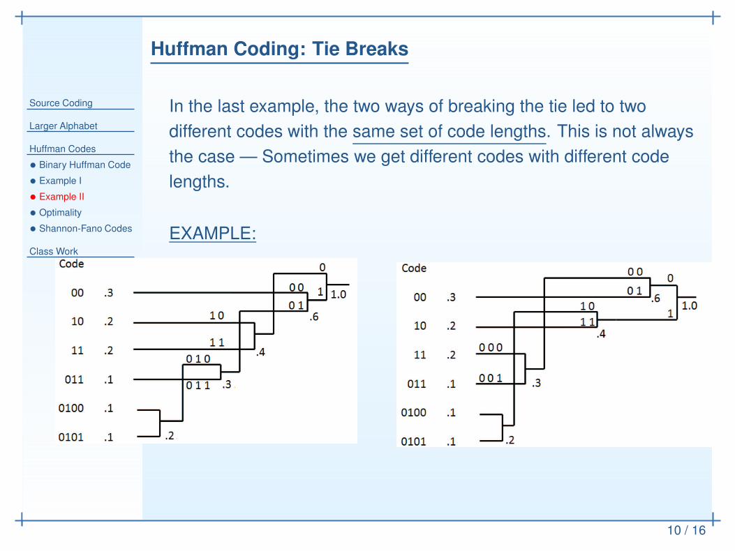
In the last example, the two ways of breaking the tie led to two

different codes with the same set of code lengths. This is not always

the case — Sometimes we get different codes with different code

lengths.

EXAMPLE:

Huffman Coding: Optimal Average Length

Source Coding

Larger Alphabet

Huffman Codes

• Binary Huffman Code

• Example I

• Example II

• Optimality

• Shannon-Fano Codes

Class Work

11 / 16

• Binary Huffman Code will have the shortest average length as

compared with any U.D. Code for set of probabilities (No U.D. will

have a shorter average length).

◦ The proof that a Binary Huffman Code is optimal — that is,

has the shortest average code word length as compared with

any U.D. code for that the same set of probabilities — is

omitted.

◦ However, we would like to mention that the proof is based on

the fact that in the process of constructing a Huffman Code

for that set of probabilities other codes are formed for other

sets of probabilities, all of which are optimal.

Shannon-Fano Codes

Source Coding

Larger Alphabet

Huffman Codes

• Binary Huffman Code

• Example I

• Example II

• Optimality

• Shannon-Fano Codes

Class Work

12 / 16

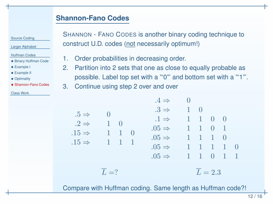
SHANNON - FANO CODES is another binary coding technique to

construct U.D. codes (not necessarily optimum!)

1. Order probabilities in decreasing order.

2. Partition into 2 sets that one as close to equally probable as

possible. Label top set with a ”‘0”’ and bottom set with a ”‘1”’.

3. Continue using step 2 over and over

Shannon-Fano Codes

Source Coding

Larger Alphabet

Huffman Codes

• Binary Huffman Code

• Example I

• Example II

• Optimality

• Shannon-Fano Codes

Class Work

12 / 16

SHANNON - FANO CODES is another binary coding technique to

construct U.D. codes (not necessarily optimum!)

1. Order probabilities in decreasing order.

2. Partition into 2 sets that one as close to equally probable as

possible. Label top set with a ”‘0”’ and bottom set with a ”‘1”’.

3. Continue using step 2 over and over

.5 ⇒ 0

.2 ⇒ 1 0.15 ⇒ 1 1 0.15 ⇒ 1 1 1

.4 ⇒ 0

.3 ⇒ 1 0

.1 ⇒ 1 1 0 0.05 ⇒ 1 1 0 1.05 ⇒ 1 1 1 0.05 ⇒ 1 1 1 1 0.05 ⇒ 1 1 0 1 1

L =? L = 2.3

Compare with Huffman coding. Same length as Huffman code?!

More Examples

Source Coding

Larger Alphabet

Huffman Codes

Class Work

• More Examples

• More Examples

• More Examples

13 / 16

Binary Huffman Codes

Source Coding

Larger Alphabet

Huffman Codes

Class Work

• More Examples

• More Examples

• More Examples

14 / 16

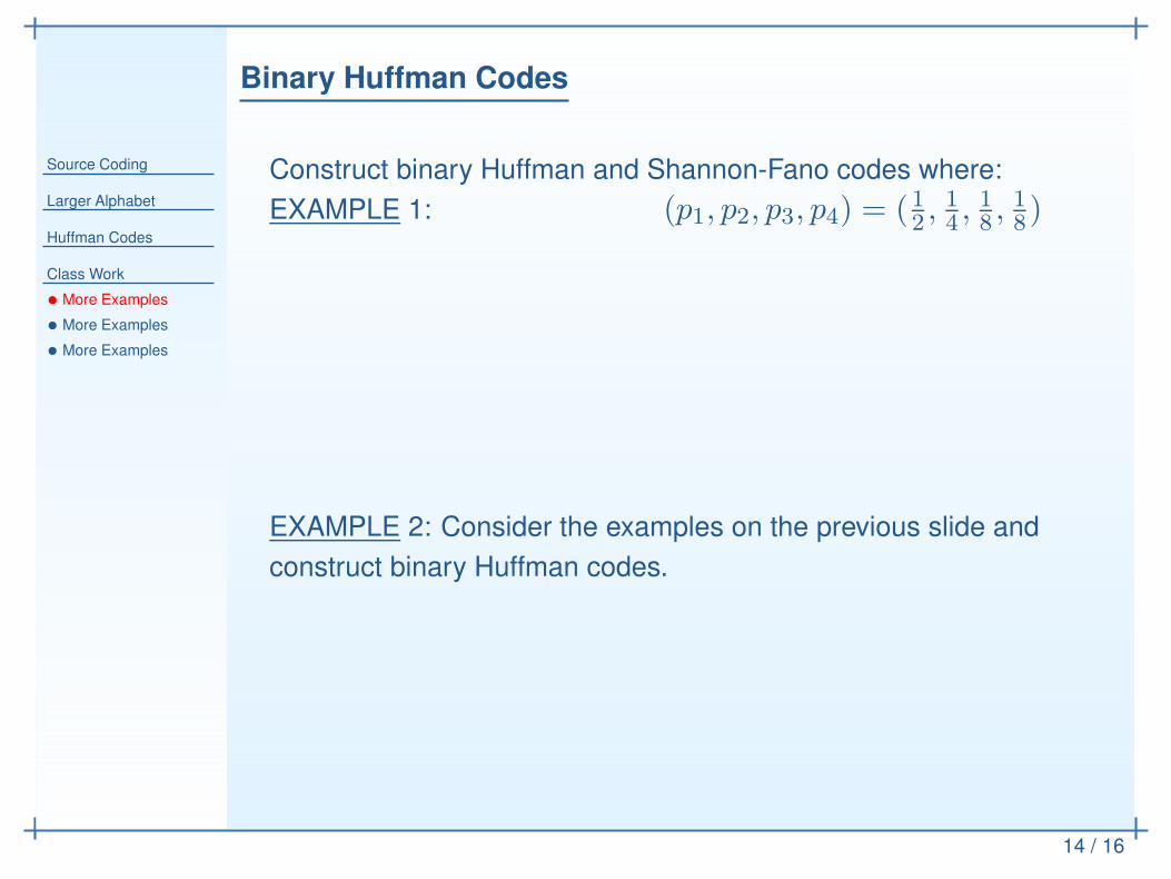
Construct binary Huffman and Shannon-Fano codes where:

EXAMPLE 1: (p1, p2, p3, p4) = (12, 14, 18, 18)

EXAMPLE 2: Consider the examples on the previous slide and

construct binary Huffman codes.

Large Alphabet Size

Source Coding

Larger Alphabet

Huffman Codes

Class Work

• More Examples

• More Examples

• More Examples

15 / 16

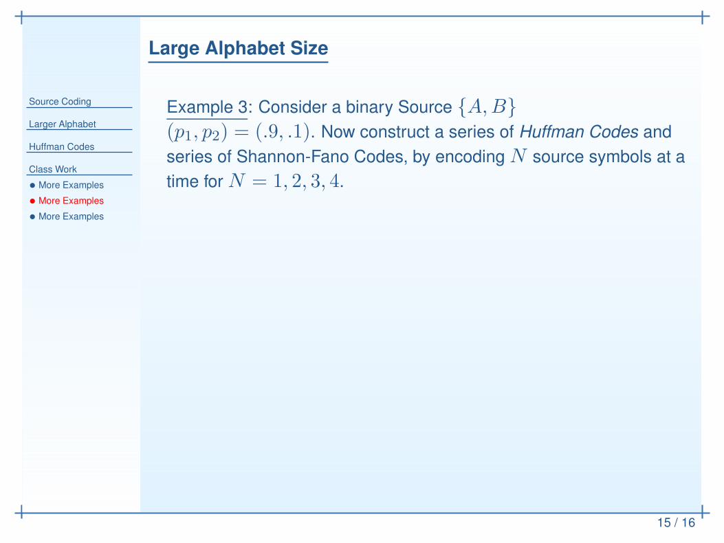
Example 3: Consider a binary Source {A,B}(p1, p2) = (.9, .1). Now construct a series of Huffman Codes and

series of Shannon-Fano Codes, by encoding N source symbols at a

time for N = 1, 2, 3, 4.

Shannon-Fano codes are suboptimal !

Source Coding

Larger Alphabet

Huffman Codes

Class Work

• More Examples

• More Examples

• More Examples

16 / 16

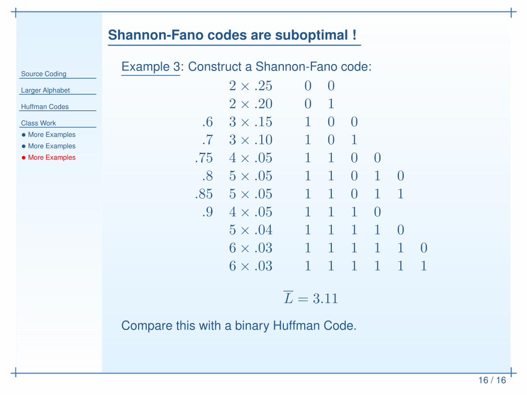
Example 3: Construct a Shannon-Fano code:

2× .25 0 02× .20 0 1

.6 3× .15 1 0 0

.7 3× .10 1 0 1.75 4× .05 1 1 0 0.8 5× .05 1 1 0 1 0

.85 5× .05 1 1 0 1 1.9 4× .05 1 1 1 0

5× .04 1 1 1 1 06× .03 1 1 1 1 1 06× .03 1 1 1 1 1 1

L = 3.11

Compare this with a binary Huffman Code.