Embed Size (px)
Citation preview

THE BRANCHING DIFFUSION APPROXIMATION FOR A
MODEL OF A SYNCHRONIZED QUEUEING NETWORK
N.G. Du�eld
AT&T Laboratories,
Room 2C-323, 600 Mountain Avenue, Murray Hill, NJ 07974, USA.
E-mail: [email protected]
M. Kelbert
The European Business Management School, University College Swansea, UK, and
International Institute for The Earthquake Prediction Theory and Mathematical
Geophysics, The Russian Academy of Sciences, Moscow, Russia.
E-mail: [email protected]
Yu.M. Suhov
Statistical Laboratory, DPMMS, University of Cambridge and St John's College,
Cambridge, UK and Institute for Problems of Information Transmission, The
Russian Academy of Sciences, Moscow, Russia.
E-mail: [email protected]
We consider a model of a centralized network under arrival-synchronization con-
straints. The mean-�eld and di�usion approximation limits are performed and it is
shown that the limiting waiting time process is described in terms of a branching
di�usion. Relations with travelling-wave solutions to a non-linear PDE are also
established.
1 Introduction
In this paper we consider a queueing network model under an arrival-
synchronization constraint. The model leads to a higher-order Lindley equa-
tion
11
. The network has N input nodes I
1
; : : : ; I
N
which are fed with inde-
pendent Poisson ows �
1
; : : : ; �
N
of intensity �. All tasks arriving in the input
ows �
j
have i.i.d. service times with some distribution F . In addition, the
tasks are provided with i.i.d. labels indicating a `type". The labels are as-
sumed to be independent on the lengths. The labels are pairs (0; k) and (1; k),
k = 1; : : : ; N , the value (0; k) being taken with probability (1�p)=N and (1; k)
being taken with probability p=N .
We describe the network operation recursively as follows. A task arriving
in ow �
j
waits �rst until all tasks arrived earlier in this ow have left the
network. Then at this time if the task has label (0; k) it is serviced (for the
duration of its service time), and leaves the network thereafter. If its label is
(1; k), the task also has to wait until all tasks with labels (0; k) and (1; k) which
1

arrived earlier in any of the ows �
j
0
, j
0
6= j, have left the network. Only after
this further waiting period is the task serviced; then it leaves the network.
Tasks with label (0; k) can be regarded as having being privileged in the
sense that before being serviced they only wait for tasks with earlier arrival
times in their input streams to leave the network. Let us call all other tasks
unprivileged.
The network rule just described may be classi�ed as an arrival-
synchronization constraint. Models this sort arise naturally in parallel process-
ing when a network deals with programs of several types which are processed
in di�erent nodes. Some types of program require information that becomes
available only after the processing of all programs of a certain type (perhaps
the same type) which were created earlier in all other nodes. Furthermore, pro-
grams created at a given node must be processed in the order of their creation.
A review of properties of networks with synchronization constraints may be
found in
4
.
To be more speci�c, we give below a concrete example of the network
that leads to this model. This example is related to a star-like network where,
in addition to the input nodes I
1
; : : : ; I
N
; there is a central node, C; and a
collection O
1
; : : : ; O
N
of the output nodes.
One may think of the tasks as programmes being processed at the input
nodes in which they are created. However, the results of processing the pro-
grams with labels (0; k) and (1; k) are collected in node O
k
(we assume that
the results are transmitted through the network without delay). A program
with label (0; k) starts processing as soon as all programs created at the same
node earlier are terminated. A program with label (1; k) has in addition to
wait until all programs labelled (0; k) or (1; k) and created earlier, no matter
in which node, are terminated. The running time of a program is, as before,
equal to its service time.
A speci�c feature of the network under consideration is that some tasks
with label (1; k) have two predecessors. One of these predecessors is the previ-
ous task to arrive in the same ow �
j
; the other is the previous task with the
same label to arrive at any input node. (Sometimes these two predecessors are
from the same ow �
j
, or may even coincide). Each of these predecessors may
have its own pair of predecessors, and so on. This creates a rather intricate
picture, and all we can do is to establish su�cient conditions under which the
network possesses stationary regimes and prove that these regimes are, in some
sense, unique.
However, there are some natural approximation schemes available which
allow us to simplify the probabilistic picture for both models. In particular,
we study in this paper an asymptotic distribution of the random process rep-
2

resenting the overall waiting times for the whole sequence of tasks arrived at
a single node I
j
(for de�niteness, we consider below the input node I
1
). More
precisely, we perform two limiting procedures: (i) N ! 1 and (ii) � ! 1,
F ) � (� is the Dirac measure) and p ! 0, with �
2
Var s, �
3=2
(�
�1
� Es)
and �p tending to �nite (positive) limits. Here and below E and Var denote
the expectation and the variance (we omit the indication of the probability
distribution if there is no confusion about this). The �rst limiting procedure is
known as the mean-�eld limit (see
3;7;11
); for the model under consideration it
results in a speci�c decoupling phenomenon between the nodes which in turn
leads to what was called in
11
a second-order Lindley equation. The second
procedure represents the well-known di�usion approximation (see, e.g.
2
, for
the model under consideration. As a result of these procedures, we pass to a
description in terms of branching di�usion processes where the independently
movingBrownian particles occasionally give birth to the new generations which
then proceed in a like manner.
Branching di�usion processes (in their simplest version) were studied in
17
in connection with the Kolmogorov{Petrovskii{Piskunov (KPP) equation
16
, a non-linear PDE that plays an important role in various applications (see,
e.g
10
]). This process has been intensively studied since (see, e.g.
5;6;9
and the
references therein), but to our knowledge a branching di�usion process only
recently appeared directly in a queueing network context (cf.
8
). Our result
relates the virtual waiting time distribution function in an overloaded network
with the travelling wave solution to the KPP equation.
2 The Models, Results and Main Probabilistic Constructions
2.1 The models: a formal description.
As was said, the random times t
(j)
n
, n = 0;�1; : : :, of tasks' arrivals at the
input node I
j
, j = 1; : : : ; N , form a Poisson ow �
j
of intensity � (as usually,
t
(j)
0
denotes the �rst point from �
j
on R
+
, the non-negative half-axis). We can
think of �
j
as a marked random ow, with i.i.d. marks (s
(j)
n
; a
(j)
n
) where s
(j)
n
is
the length and a
(j)
n
is the label of the n
th
task arrived in �
j
. The components
s
(j)
n
and a
(j)
n
are also independent, and s
(j)
n
takes values in R
+
according to the
distribution F . The label a
(j)
n
takes the values (0; k) and (1; k), k = 1; : : : ; N ,
with probabilities (1 � p)=N and p=N , respectively.
We therefore can form, for each k = 1; : : : ; N , a ow �
k
composed by
the times of arrival of the tasks with labels (0; k) and (1; k) regardless of the
input node of each task. Let us denote the points from ow �
k
by
�
t
(k)
m
, m =
3

0, �1;�2 : : : . We associate elements of the ows as follows. With a task
arriving in input ow �
j
at time t
(j)
n
with labels (0; k) and (1; k), k � 1, one
can associate an integer m = m(n; j; k) indicating the place of epoch t
(j)
n
in
the realization of the corresponding ow �
k
. In other words,
t
(j)
n
=
�
t
(k)
m
; provided that a
(j)
n
= (�; k): (1)
We can also `transfer' to the ow �
k
the service times of the corresponding
tasks. The service time of a task that has appeared in ow �
k
at time
�
t
(k)
m
is
denoted by �s
(k)
m
:
�s
(k)
m
= s
(j)
n
if
�
t
(k)
m
= t
(j)
n
: (2)
This enables us to think of the �
k
's as marked random ows. As follows
from the description provided above, ows �
k
are independent marked Poisson
ows of intensity � with i.i.d. marks. Of course, the �
k
's are functions of the
�
j
's, in the sense that ows �
k
are de�ned on the probability space formed
by the collections of the realizations of ows �
1
; : : : ; �
N
, with the probability
distribution P
N
that is the direct product of the distributions of ows �
j
.
Denote by w
(j)
n
( respectively �w
(k)
m
) the waiting time for the task that
arrives at time t
(j)
n
in ow �
j
(respectively, appears at time
�
t
(k)
m
in ow �
k
).
The network operating rule described in the introduction leads to the following
recursive equations
w
(j)
n
=
8
>
>
>
>
>
<
>
>
>
>
>
:
max[0; w
(j)
n�1
+ s
(j)
n�1
� (t
(j)
n
� t
(j)
n�1
)];
if a
(j)
n
= (0; k); 1 � k � N ,
max[0; w
(j)
n�1
+ s
(j)
n�1
� (t
(j)
n
� t
(j)
n�1
);
�w
(k)
m�1
+ �s
(k)
m�1
� (
�
t
(k)
m
�
�
t
(k)
m�1
)];
if a
(j)
n
= (1; k); 1 � k � N:
(3)
Our �rst result is about the existence of a stationary regime in the model
under consideration. Su�cient condition that becomes asymptotically tight in
the mean-�eld limit (see below) is given in Proposition 2.1. It is convenient to
introduce a (2�2) matrix
A(a) =
0
B
@
�(1� p)
�+ a
Ee
as
2�p
� + a
Ee
as
�(1� p)
�+ a
Ee
as
2�p
� + a
Ee
as
1
C
A
: (4)
Here a > 0 is a parameter. The matrixA(a) re ects a speci�c character of the
random processes describing the stationary regime: it has a transparent mean-
ing in the context of a random �eld on a Cayley tree-graph whose connection
4

with the current problem we elaborate below. The norm of A(a) is equal to
�
� + a
(1 + p)Ee
as
: (5)
Proposition 2.1 For all N , under the condition
inf
a>0
jjA(a)jj < 1 (6)
the system of equations (3) has, for P
N
-almost every array ft
(j)
n
; s
(j)
n
; a
(j)
n
g, a
solution that is unique in a class of the sequences fw
(j)
n
g satisfying the following
condition of boundedness (in probability):
lim
y!1
sup
n
P
N
(w
(j)
n
> y) = 0: (7)
If we concatenate the components w
(j)
n
to pairs (s
(j)
n
; a
(j)
n
) constituting the
marks in ows �
j
, the resulting family of extended ows
�
�
j
, 1 � j � N , is
stationary in time.
2.2 The mean-�eld approximation: limiting stochastic equations.
The extended families f
�
�
j
g mentioned in Proposition 2.1 describe the working
regimes in our network: any network characteristic may be, in principle, found
from the joint probability distributions of ows
�
�
1
; : : : ;
�
�
N
, which we denote by
�
P (
�
P
N
): However, the trouble with distribution
�
P is that it contains a lot of
dependences (it is not the product of the marginal distributions of ows
�
�
j
) and
does not provide any opportunity for a (non-trivial) explicit calculation. To
simplify we take the limit N !1 (see
11
). Under our assumptions, this limit
is analogous to the mean-�eld limit in Statistical Physics in the sense that
in this limit individual tasks wait for service in an independent background
created by other tasks in the network. The limiting stationary distribution of
w
(j)
, for a �xed j (say j = 1), exists and is identi�ed as a minimal solution to
the following stochastic equations
w ' max[0; w
0
+ s
0
� l
0
; �(w
00
+ s
00
� l
00
)]: (8)
Here ' means equality in law, and the random variables w
0
and w
00
in the
RHS of (8) have the same distribution as w. We denote this distribution which
solves (8) by �. We also denote by � the corresponding distribution function.
Further on s
0
and s
00
in (8) have the distribution F , l
0
and l
00
are exponentially
distributed with mean �
�1
, and � takes value zero with probability 1� p and
5

one with probability p. Finally, all random variables in the RHS of (8) are
independent.
It turns out (see
13
) that, under the condition (6) the solution to the
equations (8) exists, but is non-unique, however small � or Es. (Actually,
condition jjA(a)jj � 1 is su�cient for this. It is also necessary (see below)).
Under condition (6), there exists a linearly ordered continuum of solutions of
(8), with di�erent asymptotics of �(x) as x!1. (Here we mean the standard
stochastic order: for random variables u
0
and u
00
with distribution functions
�
0
, �
00
the partial order u
0
� u
00
means �
0
(x) � �
00
(x), x 2 R
1
). There exists a
unique minimal solution, �
0
, corresponding to the `zero initial condition' that
initial waiting times are zero:
w
(j)
0
= 0; 1 � j � N: (9)
If on the other hand kA(a)k > 1 for all a > 0 then equation (8) has no solution
in the set of proper distribution functions. However, equation (3) may be
iterated from some initial condition (say the zero condition). This gives us a
family of extended ows
�
�
+
j
, 1 � j � N , which are de�ned on the non-negative
half-axis. The limit N !1 may also be performed in this case.
Let us concentrate now on the structure of the sequence w
(j)
n
for a �xed
value of j. We consider the case j = 1 and omit, for simplicity, index 1
writing � and
�
� instead of �
1
and
�
�
1
, �
+
and
�
�
+
instead of �
+
1
and
�
�
+
1
, etc).
Consider �rst the case where the conditions of Proposition 2.1 are ful�lled. As
was said before, the extended ow
�
�, with marks (s
(j)
; a
(j)
); describes, for a
given N , the stationary regime in the input node I
1
. It is convenient to pass
to the reduced labels of the tasks arrived, by setting a
�
n
= 0, if a
n
= (0; k)
and a
�
n
= 1, if a
�
n
= (1; k), 1 � k � N . The corresponding reduced ows
with marks (s
n
; a
�
n
; w
n
) may be denoted as �
�
and
�
�
�
, respectively. The new
components of the mark a
�
n
are (conditionally) i.i.d. and take their values 0
and 1 with probability 1 � p and p, respectively. Our results about the limit
N !1 for the model under consideration are summarized in the Theorem 1
following. Hereafter the notion of covergence we use is of a vague convergence
of random processes, i.e. the convergence of the expectation values of bounded
continuous local functions on the realization space of the process. The precise
de�nition depends on the topology on this space, and we formally introduce it
when we prove the corresponding theorem.
Theorem 1 Under condition (6), the extended ow
�
�
�
converges, as N !1,
to a limiting ow �
�
which is characterised in an unique way by the following
conditions:
(i) The times t
n
and the components of the mark s
n
and a
�
n
, n = 0;�1; : : :,
are distributed as in ow �
�
.
6

(ii) Given a sequence f(t
n
; (s
n
; a
�
n
)); n = 0;�1; : : :g, the sequence fw
n
; n =
0;�1; : : :g satis�es the recursive equations
w
n
=
8
<
:
max [0; w
n�1
+ s
n�1
� (t
n
� t
n�1
)]; if a
�
n
= 0;
max [0; w
n�1
+ s
n�1
� (t
n
� t
n�1
); ew
n
+ es
n
� L
n
];
if a
�
n
= 1,
(10)
where ew
n
; es
n
; L
n
, n = 0;�1; : : :, are independent random variables, ew
n
has distribution �
0
, es
n
has distribution F and L
n
is exponentially dis-
tributed with mean �
�1
.
We can split the distribution �
0
of the minimal solution w to (8) into
two parts: �
0
= (1 � p)�
0
1
+ p�
0
2
where, with the notation of (8), �
0
1
is the
distribution of the random variable max[0; w+s� l] and �
0
2
the distribution of
max[0; w
0
+ s
0
� l
0
; w
00
+ s
00
� l
00
]. Then the marginal (conditional) distribution
of the component of the mark w
n
in the limiting ow in Theorem 1 is �
0
1
when
a
�
n
= 0 and �
0
2
when a
�
n
= 1: (The precise formulation of this assertion requires
the use of a Palm distribution. This will become more transparent when we
pass to the di�usion approximation).
2.3 Random Processes on Random Trees
We now associate to solutions of (8) random processes on random trees. This
will be used in proving the validity of mean-�eld and di�usion limits (see
Theorems 2{4 below). Consider the Cayley tree rooted at an origin O, and
with branching ratio 2. Each edge e can be identi�ed with a binary sequence,
which also identi�es its vertex furthest from the origin. (The origin is then
identi�ed with the null sequence). Denote by L
0
the set of �nite continuous
paths starting at the origin: clearly each path L 2 L
0
is identi�ed with its
�nal edge (or equivalently its �nal vertex) and hence is given again by a �nite
binary sequence. In a random tree on the other hand the branching ratio is
random at each vertex, but maximally 2. We use various equipments of trees,
these being the association of random variables (i.e. marks) with each of the
edges of the tree.
We now associate with the solution to equation (8) a random process fw
e
g
on the edges (or equivalently the vertices) of a random tree which possesses a
natural stationarity property. The basic idea here is that each edge is associ-
ated with a task, and that adjacent edges above (or o�spring) correspond to
the predecessors of this task. Hence in this case each edge of the tree spawns
one o�spring with probability 1� p and two with probability p, independently
of other edge. To each edge e we assign a pair of random variables l
e
, s
e
where
s
e
has distribution F and l
e
has the exponential distribution with mean �
�1
:
7

The assumption of the (conditional) independence of the whole array l
e
; s
e
is
of course preserved.
We specify the random variables fw
e
g to be related by a recursive system
of equations similar to (3) above, namely
w
e
=
8
<
:
max[0; w
~e
+ s
~e
� l
~e
] if e has one o�spring,
max[0; w
~e
0
+ s
~e
0
� l
~e
0
; w
~e
00
+ s
~e
00
� l
~e
00
];
if e has two o�spring.
(11)
Then minimal solution �
0
will be identi�ed with the distribution of the quan-
tity
max[0; sup
L2L
0
X
e2L
(s
e
� l
e
)]: (12)
In the random-tree picture, then the component �
0
1
gives the conditional dis-
tribution under the condition that the initial vertex O creates one o�spring,
and the component �
0
2
the conditional distribution under the condition that
O creates two o�spring.
2.4 The di�usion approximation.
The di�usion approximation we consider in this paper is related to the process
of the virtual waiting time v(� ), � 2 R, generated by the queueing in our input
node I, in the limiting extended ow �
�
:
v(� ) = max[0; w
bn
� (� � t
bn
)] (13)
where bn is de�ned by the requirement that t
bn
is the �rst arrival time in ow
�
�
which precedes � . Under the conditions of Theorem 1, this is a station-
ary, continuous-time regenerative process. The resulting process is complex
(although parameters may be determined from Theorem 1). We obtain a
simpler picture in terms of branching di�usion by making an approximation
in which the intensity of the random ow
�
�
�
(or �
�
) becomes large and the
random variables s
n
become negligibly small.
Let us �rst describe the limiting di�usion. Consider a family of Brownian
particles, each particle having a type 1 or 2 and moving independently on a
line. The drift coe�cient of a particle of type i is �
i
and its di�usion coe�cient
is �
i
, i = 1; 2. After independent exponential lifetimes, with the mean values
�1
1
and
�1
2
, respectively, the particles die, each giving birth to two o�spring,
one of type 1 and one of type 2, The descendants then proceed independently
according to their type. From
12
we have the following
8

Proposition 2.2 Let X denote the supremum of the deviation, in the positive
direction, of all particles taken over all times of particles' death. A su�cient
condition for X to have a proper distribution is:
inf
0<b<b
�
1
1
� �
1
b�
�
2
1
2
b
2
+
2
2
� �
2
b�
�
2
2
2
b
2
!
< 1; (14)
where b
�
is de�ned as the supremum of those values of
e
b > 0 for which
both denominators in the expression under the in�mum are positive for any
b 2 (0;
e
b):
We shall obtain these di�usions by taking the following limit:
�!1; �
2
Var
F
s! r � 0; �
3=2
(E
F
s � �
�1
)! ' 2 R; �p! > 0 (15)
subject to the technical condition
E
F
s
2+�
� C; (16)
with �xed constants �;C 2 (0;1): In our model we will set �
1
= �
2
= ',
1
=
2
= and �
1
= �
2
= � := (1 + r)
1=2
, condition (14) becoming that
' < 0 ; '
2
=�
2
> 2 : (17)
We actually need not distinguish between the di�erent types of particle due to
the identify of their parameters.
We can represent the branching di�usion as a random process, now on a
non-random rooted Cayley tree with �xed branching ratio 2. Roughly speak-
ing, the correspondence with the random trees in the previous section is that
the vertices of the �xed tree correspond to those vertices on the random tree
where branching with ratio 2 actually takes place. We equip each edge e with
an independent random pair (g
e
; S
e
), where g
e
is distributed exponentially
with mean
�1
, while S
e
is a Wiener trajectory on [0; g
e
) with drift coe�cient
' and di�usion coe�cient �.
The distribution of the random quantity
max [ 0; sup
L2L
0
X
e2L
S
e
(g
e
) ] (18)
may be identi�ed with the distribution of the variable X of Proposition 2.2
(which justi�es the use of the same symbol X in the notation). The distribution
of X is denoted by
�
�
0
. As before, we have a pair of distributions,
�
�
0
1
and
�
�
0
2
according to whether we have one or two particles present initially.
9

Physically speaking, we perform in (18) an operation of `glueing' the tra-
jectories S
e
along a path L and then compute the �nal displacement from the
origin.
In fact we only need to know the second component, since if for example
X
2
has distribution
�
�
0
2
, then
max[0; X
2
+ S] (19)
has distribution
�
�
0
1
, where S is the displacement of independent Wiener par-
ticle, with the drift coe�cient ' and the di�usion coe�cient �, at the random
stopping time that is exponentially distributed, with mean
�1
:
As before, we can write stochastic equations analogous to (10) or, in the
stationary form, to (8). The analogue of the second equation in (10) is
W
�
= max [ 0;W
�
0
+ S(g
e
0
);W
�
00
+ S(g
e
00
) ]; (20)
and the analogue of (8) is
W ' max [ 0;W
0
+ S(g
0
); W
00
+ S(g
00
) ]; (21)
we retained here the same rules of the notation and the conventions about
the distributions as in (9) and (8). Under condition (17) the minimal solution
�
�
0
2
to (21) is unique and is a proper probability distribution. However, there
exists again a linearly ordered continuum of solutions distinguishable in their
behavior at in�nity (see
12
).
Our result on the di�usion approximation is as follows:
Theorem 2 Suppose that �, F and p are varied as indicated in (15), so that
conditions (6), (16) and (17) hold true. Then, the random process fv(� ); � 2
R
1
g, converges to a stationary process, fV (� ), � 2 R
1
g: The distribution of
fV (� ), � 2 R
1
g is the marginal distribution of the second component in a pair
(�; f
e
V (� ), � 2 R
1
g); where � is a stationary Poisson process of intensity
: The conditional distribution of process f
e
V (� ), � 2 R
1
g; given a realization
f�
�
n
; n 2 Zg; of process �; is characterized as follows. (a) The trajectories of
the conditional process (which we denote by f
e
V (� jf�
�
n
; n 2 Zg ) are continuous
on R
1
n f�
�
n
; n 2 Zg; on f�
�
n
; n 2 Zg they are right-continuous and have left
limits; (b) The process f
e
V (� jf�
�
n
; n 2 Zg)g possesses the following Markov
cyclicity property: for any j 2 Z; the conditional distribution of the random
variables
e
V (� jf�
�
n
; n 2 Zg), � 2 (�
�
j
; �
�
j+1
); given the past
e
V (� jf�
�
n
; n 2 Zg),
� < �
�
j
; depends on the value
e
V (�
�
j
jf�
�
n
; n 2 Zg) only, and is given by
e
V (� jf�
�
n
; n 2 Zg) = max [ sup
�
�
j
<t��
S(��t);
e
V (�
�
j
jf�
�
n
; n 2 Zg)+S(���
�
j
)]; (22)
10

where S(u)(= S
(�
�
)
(u)), u � 0, is the time-homogeneous Wiener process
with the drift coe�cient ' and the di�usion coe�cient �, independent on
e
V (e� jf�
�
n
; n 2 Zg), e� � �
�
j
. c) The values
e
V (�
�
j
jf�
�
n
; n 2 Zg), j 2 Z, at the
initial points of the cycles are given by
e
V (�
�
j
jf�
�
n
; n 2 Zg) = max [
e
V (�
�
j
� 0jf�
�
n
; n 2 Zg); Y
j
]; (23)
where Y
j
are i.i.d random variables, and each variable Y
j
has distribution
�
�
2
emerging in the model of the branching di�usion.
The distribution of V (� ) at a (non-random) time � coincides with
�
�
0
1
.
2.5 The half-axis picture.
If we do not assume the condition (6) to hold, we are able to establish similar
pictures on the non-negative half-axis [0;+1). It is again convenient to pass
to the reduced ows �
+
�
and
�
�
+�
. Recall that initial condition (9) is supposed
to be ful�lled. In order to describe the situation, we have to introduce `cut-o�'
analogues of the constructions of the processes on trees used before.
We want to construct a `piece' of a (random) tree which has been grown
during a given time
e
t > 0: Take a realization of the tree and equip it with the
pairs of the random variables (l
e
; s
e
) according to the rule described above.
Given a collection of the values fl
e
g; consider a part of the tree con�ned to
those vertices � for which the sum
P
ee2L
�
l
ee
<
e
t: Here L
�
denotes the path
from L
0
leading to vertex �: Assign to the `border' vertices the value w
�
=
0 and compute the values w
�
for the preceding vertices via equations (10).
Equivalently, compute the maximum of the sums
P
e2L
(s
e
� l
e
) over the paths
L 2 L
0
for which
P
e2L
l
e
<
e
t: We obtain a pair of probability distributions
�
0
1
(
e
t) and �
0
2
(
e
t) describing the conditional distributions of the random variable
w
O
under the condition that the origin O has, correspondingly, one or two
o�spring.
An analogue of Theorem 1 in the half-axis picture is:
Theorem 3 The random ow
�
�
+�
converges, as N ! 1, to a limiting ow
(�
+
)
�
on the non-negative time half-axis R
+
. The distribution of ow (�
+
)
�
is characterized, in a unique way, by the following conditions:
(i) the times t
n
and the components of the mark s
n
and a
�
n
, n = 0;�1; : : :,
are distributed as in ow �
+
;
(ii) given a sequence f(t
n
; (s
n
; a
�
n
)); n = 0; 1; : : :g, sequence fw
n
; n = 1; 2 : : :g
satis�es recursive equations (10) where ew
n
; es
n
; L
n
, n = 0;�1; : : :, are
again independent random variables, ew
n
now has distribution �
0
2
(t
n
) and
11

es
n
and L
n
have, as before, distribution F and the exponential distribution
with mean �
�1
, respectively.
As in the case of Theorem 1, we can say that the marginal (conditional)
distribution of the component of the mark w
n
in the limiting ow in Theorem
3 coincides with �
0
1
(t
n
) when a
�
n
= 0 and with �
0
2
(t
n
) when a
�
n
= 1:
Theorem 4 (see below) deals with the process of the virtual waiting time
v
+
(� ), � 2 [0;1), generated by the queueing in the input node I under the zero
initial condition (9). More precisely, we perform the di�usion approximation
limit (15), now without assumptions (17). Again, in order to describe the
situation, we have to consider the cut-o� versions of the branching di�usion
process described before. This may be done on the base of the construction
of the corresponding cut-o� non-random tree. As before, �x
e
t > 0: Take
an in�nite tree that starts with two edges and equip it with the pairs (g
e
; S
e
).
Then, given a collection fg
e
g; con�ne ourselves to those vertices � for which the
sum
P
ee2L
�
g
ee
is <
e
t: Compute the valueW
O
via the cut-o� version of formulas
(20). We get a probability distribution
�
�
0
2
(
e
t). If we modify the construction
allowing the tree to start with a single edge, we obtain distributions
�
�
0
1
(
e
t).
Theorem 4 Suppose that �, F and p are varied as indicated in (15). Then
the random process fv
+
�
; � � 0g converges to a (non-stationary) regenerative
process, fV
+
(� ), � � 0g, which is characterized by conditions a), b) and c)
from Theorem 2 and the following condition.
d
0
) At the epoch of regeneration, �
�
, the process takes the value max
[V
+
(�
�
�), Y
+
(�
�
)]; where Y
+
(�
�
) is a random variable with distribution
�
�
0
2
(�
�
); which is independent on V
+
(� ), � < �
�
:
e
0
) The distribution of V (� ) at a (non-random) time t coincides with
�
�
0
1
(� ):
2.6 A travelling wave bound.
Under the condition opposite to (6)
inf
a>0
jjA(a)jj > 1; (24)
the network does not possess a stationary regime in the mean-�eld limit. [An
expected picture is that the non-overload condition in a �nite network depends
on N and is more `liberal' than (6) (so that, for N <1, a network may have
a unique stationary regime even when (6) is violated), but in the mean-�eld
limit N ! 1 this condition coincides with (6).] In terms of the di�usion
approximation, it means that process V
+
(� ) increases to in�nity, in the
12

sense that the distribution function x 2 R
+
7! Pr (V
+
(� ) < x) vanishes, as
� !1:
It is interesting to analyze the speed of convergence of Pr(V
+
(� ) < x)
to zero and it is conjectured that a good bound is provided by the travelling
wave solution to a non-linear di�erential equation. This conjecture is based on
a connection between the branching di�usion processes and non-linear partial
di�erential equations of the so-called KPP (Kolmogorov-Petrovskii-Piskunov)
type. Our model leads to the simplest model of branching di�usion with a
single type Wiener process, and to a single KPP equation (see
16
)
@
@t
u(t; x) + �
@
@x
u(t; x) =
�
2
@
2
2@x
2
u(t; x) + u(t; x)(u(t; x)� 1); t � 0; x 2 R
1
:
(25)
The following types of solutions to (25) are of interest.
(a) Solutions of the Cauchy problem, with the initial date u(t; x)]
t=0
= �(x);
where � is the indicator function of the non-negative half-axis R
+
:
(b) Solutions that possess the travelling wave property: u(t; x) = u
�
(x �
ct); x; t 2 R
1
; parameter c 2 R
1
is called the travelling wave velocity and
the function u
�
the travelling wave pro�le (with travelling wave velocity
c).
The conjectured bound by the travelling wave is of the form Pr(V
+
(t) <
x) � u
0
(x � m(t)); where u
0
is the travelling wave pro�le corresponding to a
minimal possible velocity c
0
> 0; and lim
t!1
t
�1
m(t) = c
0
.
Proposition 2.3 Under the condition
�
2
=�
2
> 2 (26)
the solution u(t; x) of the Cauchy problem with the initial date �(x) satis�es
the following bound: for t > T (x)
u(x; t) � u
0
(x�m(t)); x 2 R
1
: (27)
Here, u
0
(x) is the (unique) travelling wave pro�le that corresponds to the min-
imal velocity c
0
= 2
1=2
� + � and obey u
0
(0) = 1=2 and
m(t) = c
0
t+ logt + o(logt): (28)
The function u
0
(x) is exponentially decreasing at �1:
lim
x!�1
logu
0
(x)
x
= � < 0; (29)
and threshold T (x) obeys T (x) � max[Ax;B]; where A;B > 0 are constants.
13

For the proof of Proposition 2.3, see
17
. We prove the following result in
section 5.
Theorem 5 Under condition (26),then for x > 0 and t > T (x)
Pr(V
+
(t) < x) � u
0
(x�m(t)): (30)
The bound (30) illustrates the behaviour, as t ! 1, of process V
+
(t)
and hence the limiting behavior of original waiting time process v
+
(t), in the
overloaded system (we mean here the di�usion approximation limit of v
+
(t)).
In particular, bound (30) implies that Pr(V
+
(t) < x) decreases exponentially
in t as t!1.
3 Convergence to the mean-�eld limit
3.1 The basic construction: Proof of Proposition 2.1
Theorem 1 may be derived from Proposition 2.1 (or, more precisely, from an
argument the proof of this proposition is based upon). Thus, we concentrate on
the proof of Proposition 2.1 and complete the proof of Theorem 1 afterwards.
The proof of Proposition 2.1 is split into two steps: (i) the construction of a
family of extended ows
�
�
>t
0
j
; 1 � j � N; on a time half-axis t
0
+R
+
= [t
0
;1)
with, say, the zero initial condition at time t
0
; and (ii) the proof of the existence
of the limit of family
�
�
>t
0
when t
0
! �1: As noted before, the �rst step is
merely a straightforward iteration of equation (3).
As to the second step, it is based on an innovation event method going
back to works of Borovkov (see
1;2
). In our context, this method exploits a
detailed analysis of a `predecessor picture', for a given task, as this picture
develops backwards in time. A basic component of the predecessor picture is
a compatible family of oriented random graphs (called predecessor graphs),
associated with the task arriving in ows �
j
after time t
0
. The predecessor
graph associated with a given task indicates the numbers and the types of its
subsequent predecessors (the number of outgoing edges from any vertex of the
predecessor graph is always equal to 1 or 2).
Speaking of a given (or `tagged') task, we mean a �xed pair (j
0
; n
0
) and
pick the n
0
-th successive task in ow �
>t
0
j
0
= �
j
0
�
�
t
0
+R
+
, the restriction of the
original input ow �
j
0
to [t
0
;1). The construction of the predecessor graph
begins with a `root' which is denoted again by O; the root is associated with
a tagged task. The number of the edges going out of O equals one if the
component of the mark a
n
0
= (0; k). In the case a
n
0
= (1; k), k � 1, the
task, generally speaking, has two predecessors, one in each of two queues. If,
14

by chance, these predecessors coincide, the corresponding edges are `glued'
together.
Thus, the vertices at the other ends of the edges are associated with the
predecessors of the tagged task. The above procedure is then repeated for these
vertices: the number of the edges going out of them are de�ned in the same
fashion, depending on their marks, and glueing occurs when their predecessors
coincide. The procedure is then again repeated for the `next' predecessors,
etc. As a result, we end up with an oriented graph �
>t
0
(j
0
;n
0
)
which is obtained
from the Cayley tree, of branching ratio two, by `cutting' o� some branches
and `glueing' some edges (both procedures being random). Clearly, the graph
constructed can include some loops because di�erent tasks may share the same
predecessor in the past.
A similar procedure may be performed for any task from the restricted in-
put ows �
>t
0
j
, 1 � j � N ; by construction, the predecessor graphs arising for
di�erent tasks possess a natural compatibility property. For a �xed t
0
> �1,
the predecessor graphs eventually `stop' when we reach initial time point t
0
.
However, the construction may be carried on inde�nitely, creating `in�nitely-
extended' graphs. Given a tagged task (j
0
; n
0
), it is convenient to think of
an in�nite predecessor graph �
(j
0
;n
0
)
and a family of its `cut-o�' subgraphs
of `depth' `, ` = 1; 2; : : :. More precisely, we consider, for any ` = 1; 2; : : :, a
familyM
(j
0
;n
0
)
(`) of the paths on �
(j
0
;n
0
)
starting at O and having exactly `
edges. While speaking of a �xed tagged task, index (j
0
; n
0
) is systematically
omitted.
Observe that for any tagged task (j
0
; n
0
),
E
P
>t
0
N
jM(`)j � (1 + p)
`
: (31)
Here, jM(`)j is the cardinality of set M(`), and P
>t
0
N
is the joint probability
distribution of family f�
>t
0
j
, 1 � j � Ng; one can of course replace it with the
joint distribution
�
P
>t
0
N
of family f
�
�
>t
0
j
, 1 � j � Ng (see above).
Pictorially, the predecessor graphs absorb the whole `N -dependance' that
is present in probability distribution
�
P
>t
0
N
. To determine the predecessor
picture, we assign, to the edges e of the predecessor graph, random variables
�
e
of the form �
e
= s
e
� T
e
: Random variables s
e
and T
e
are assumed to be
independent, as for a single edge as for di�erent edges. [More precisely, s
e
and T
e
are assumed to be conditionally independent, given a realization of the
predecessor graph.]
Random variables s
e
have distribution F and random variables T
e
are
distributed exponentially, with means �
�1
.
The object we end up with (a random graph �
(j
0
;n
0
)
and an array of ran-
15

dom variables �
e
) is inferred from probability distributions
�
P
>t
0
N
(or P
>t
0
N
),
t
0
> �1, and de�nes what was called the predecessor picture. By con-
struction, the predecessor pictures obtained for di�erent tasks are compatible.
Given a tagged task (j
0
; n
0
), it is convenient to consider a continuous family
of sub-graphs of predecessor graph �, labeled by a parameter representing the
di�erence t
n
0
� t
0
between t
n
0
, the time the tagged task arrived at the network
and the initial time t
0
. More precisely, in analogy with M(`) (see above), we
consider, for any given T > 0, a (random) familyM
(T )
(j
0
;n
0
)
of the paths L, on
graph �, which start at root O and are extended up to time T backwards,
counting from t
n
0
. [It means that the sum
X
e2L
l
e
� T .]
Physically speaking, a predecessor picture characterizes a chain of events
that determines the `fate' of a given task in families of the extended ows
f
�
�
>t
0
j
g. For example, the waiting time of a tagged task (j
0
; n
0
) in family
f
�
�
>t
0
j
g is identi�ed with the random variable
max
h
0; sup
L 2 M
(t
n
0
�t
0
)
X
e 2 L
�
e
i
: (32)
Observe that the �nal part of the above construction (assigning random
variables �
e
to the edges of the predecessor graph) does not explicitly refer to
value N , as soon as a realization of the predecessor graph is �xed.
Next, we introduce an innovation event
C =
(
9`
0
2 N : 8L 2M(`); with ` � `
0
;
X
e2L
�
e
� 0
)
: (33)
We will use a standard Borel{Cantelli Lemma to check that for any N
P
>t
0
N
(C) = 1: (34)
This is based on the fact that the series
X
`
P
>t
0
N
there exists L 2M(`) :
X
e2L
�
e
> 0
!
: (35)
converges uniformly in N .
The proof of this fact is straightforward: series (35) is majorized, term by
term, by the series
X
`
E
P
>t
0
N
jM(`)j
b
P (�
`
> 0) : (36)
16

Here
b
P is the joint probability distribution of the sequence of i.i.d. random
variables of the form � = s� t, where s and t are independent and distributed
as before (s has distribution F and t an exponential distribution of mean �
�1
).
Furthermore, �
`
is the sum of ` random variables from the sequence.
By using Cherno�'s inequality we conclude that, for any a > 0,
b
P (�
`
> 0) � (E
�
exp (a�)
�
`
=
�
�
� + a
E exp (as)
�
`
: (37)
Owing to condition (6) and bound (31), there exists a > 0 that the series
(35) converges uniformly in N . By the Borel{Cantelli Lemma we conclude
that (34) is valid. Moreover, the same argument shows that the supremum in
(32) is attained at a path L that belongs to a set M
(T
0
)
(j
0
;n
0
)
(i.e. is extended
backwards up to (random) time T
0
(= T
0
(j
0
; n
0
)), from point t
n
0
), with T
0
being bounded in probability uniformly in N , j
0
= 1; 2; : : : ; N , n
0
= 1; 2; : : :,
and t
0
2 R:
lim
y!1
sup
N;j
0
;n
0
;t
0
P
>t
0
N
(T
0
> y) = 0: (38)
[In fact, given a k � 1, a similar relation holds for the random variables
�
T
0
(j
0
; n
0
; k) = max
h
T (j
0
; en
0
) : n
0
� en
0
� n
0
+ k
i
.] This allows us to control
the `memory' in extended ows
�
�
>t
0
j
, j = 1; : : : ; N , uniformly inN and perform
the limit t
0
!�1. As a result, we obtain a stationary family of extended ows
f�
j
g that solves equations (3). Finally, a coupling argument (cf.
11
) implies the
uniqueness of the solution obtained, in the class indicated in Proposition 2.1.
This completes the proof of Proposition 2.1.
3.2 Proof of Theorem 1.
The uniformity in N occurring in estimates discussed in the previous section
allows us to pass to the limitN !1. Namely, by inspecting a `cut-o�' family
M
(T )
(j
0
;n
0
)
(or M
(j
0
;n
0
)
(`)) of paths on predecessor graph �
(j
0
;n
0
)
, for a given
T > 0 (or ` � 1), one can observe that as N ! 1 the following probability
vanishes: that among tasks that are met in the course of inspection, either
(i) at least two have predecessors which are unprivileged and have coincident
labels; or
(ii) at least one serves as a predecessor for more than one task.
Physically speaking, what survives in the limit N ! 1 corresponds to the
picture described in Theorem 1: for any tagged task (j
0
; n
0
) and any T >
17

0, no branches in the T -extended piece of the original Cayley tree are cut
and no vertices are glued. The aforementioned uniformity allows us to make
this argument rigorous. In other words, all random variables emerging in the
recurrence (3) in the limit N !1 become independent. This guarantees the
existence of the limiting ow �
�
satisfying conditions (10).
4 Convergence to the di�usion limit
It is convenient to start with proving of Theorem 4. We will need minor
technicalities.
4.1 Preliminaries.
The processes fv
+
�
; � � 0g and fV
+
(� ); � � 0g live in the space D
+
of functions
� : [0;1)! R
1
; without the second-kind discontinuities. For de�niteness, let
us assume that the functions are right-continuous. We endow space D
+
with
the standard Skorokhod topology and the standard nested family of the �-
algebras D(� ), � > 0: Fix �
0
> 0 and a bounded D(�
0
)-measurable function f
: D
+
! R
1
which is continuous in the above topology. Denoting by P
+
the
probability distribution of process fv
+
�
g and by Q
+
that of process fV
+
(� )g;
we have to prove that, in the course of the limiting procedure (15),
limE
P
+f = E
Q
+f : (39)
In the course of the proof, we use directly a construction of processes
fv
+
�
g and fV
+
(� )g which is related to the non-random tree, more precisely, to
`equipments' of the tree with some random elements. To this end, we have to
introduce probability distributions P
tree
and Q
tree
of the `basic' equipped trees
for these processes. [Actually, distribution Q
tree
was in substance determined
in Section 2; the construction provided below completes the formal side of the
de�nition.] Distributions P
tree
and Q
tree
are de�ned on a �-algebra T in the
space T of the basic equipped tree realizations. A point � of space T is given
by a tree-graph, together with a collection of positive numbers g
e
assigned to
its edges e: It is convenient to agree now that the origin O of the tree creates a
single edge; any other vertex of the tree always creates two edges. The number
g
e
assigned to an edge e may be interpreted as the length of e.
The �-algebra T is generated by the variables g
e
: Both probability distri-
butions P
tree
and Q
tree
correspond to the collection of i.i.d. random variables
distributed exponentially, with means (�p)
�1
(for P
tree
) and
�1
(for Q
tree
).
The construction of process fv
+
�
g is in fact related to a re�nement of a
basic tree which may be called the `barbed' tree. We replace the random
18

variable g
e
with an ordered set l
e
= (l
e
(1); : : : ; l
e
(n
e
)) consisting of a random
number n
e
of positive random `bits'. The number of the bits is geometrically
distributed, with parameter p; and, given n
e
; their sizes l
e
(i), i = 1; : : : ; n
e
, are
i.i.d. and have the exponential distribution with mean �
�1
: The assumption of
the independence of pairs (n
e
; l
e
) for di�erent edges is retained. The space of
the barbed trees is denoted by T
�
; the corresponding �-algebra by T
�
and the
probability distribution arising by P
�
tree
: The connection between P
tree
and
P
�
tree
is established via the formula g
e
=
P
i
l
e
(i): Pictorially, a barbed tree �
�
may be associated with a basic tree where the length of each edge is partitioned
into bits.
We construct the distributions of processes fv
+
�
g; up to time �
0
; as fol-
lows. First, we perform an additional equipment of a barbed tree with the
i.i.d. copies of the random variable s assigned to each partition point z
e
(1) =
l
e
(1); z
e
(2) = l
e
(1) + l
e
(2); : : : ; z
e
(n
e
) = l
e
(1) + : : :+ l
e
(n
e
): Given the whole
array fl
e
(i), s
e
(i)g; we compute the value v
+
�
as follows. First, we extract
an (in�nite) path L
0
from the origin O and truncate it at length �
0
(we call
this path basic). Truncation means that we �x an edge e
0
= e
0
(�
0
) of L
0
and a number i
0
(= i
0
(e
0
)) (or, equivalently, the corresponding partition point
z
e
0
(i
0
)) such that
�z
e
0
(1) = �
0
�
X
e2L
0
:e�e
0
g
e
�
X
i
0
<i�n
e
0
l
e
0
(i) > 0; (40)
but
�z
e
0
(1)� l
e
0
(i
0
) < 0: (41)
Here e � e
0
means that edge e precedes e
0
on path L
0
while moving from O;
in the case i
0
= n
e
0
; the second sum in the LHS of (40) is omitted. Note the
reversed direction of labelling the partition points on the edges of the barbed
tree.
A similar truncation procedure is performed for any path from L
0
: It gives
us a collection of pairs (�e; i
0
(�e)) that, together with (e
0
; i
0
); forms a `cut' of
the barbed tree. We obtain a `truncated' tree, from O to the cut, such that
G(�e; i
0
(�e)) =
X
e2L
�e
:e��e
g
e
+
X
i>i
0
(�e)
l
�e
(i) < �
0
; (42)
but
G(�e; i
0
(�e)) + l
�e
(i
0
(�e)) > �
0
: (43)
Here, L
�e
denotes the path from L
0
that ends on �e:
19
The next step is to install the `physical' clock along the (truncated) path
L
0
. It means that we mark, on the time-interval (0; �
0
); points
�z
e
0
(1); �z
e
0
(2) = �z
e
0
(1) + l
e
0
(i
0
+ 1); : : : (44)
�z
e
0
(n
e
0
� i
0
) = �z
e
0
(1) + l
e
0
(i
0
+ 1) + : : :+ l
e
0
(n
e
0
);
then points
�z
e
1
(1) = �z
e
0
(n
e
0
) + l
e
1
(1); : : : (45)
�z
e
1
(n
e
1
) = �z
e
0
(n
e
0
) + l
e
1
(1) + : : :+ l
e
1
(n
e
1
);
etc., until we reach (at time �
0
) the origin O: Here and below e
1
denotes
the edge preceding e
0
on the truncated main path L
0
; e
2
denotes the edge
preceding e
1
; etc. Points �z
e
1
(1), �z
e
2
(1); : : : are of a special signi�cance: they
correspond the time epochs when the (truncated) barbed tree branches. Note
that the direction of the physical time is reversed with respect to the direction
in which the tree develops.
4.2 Convergence on the half-axis.
We now proceed as follows. Given � 2 (0; �
0
); we extract a part of the trun-
cated barbed tree that contains a piece of the basic path corresponding to the
time-interval (0; � ); together with all associated branches. Then set
v
+
�
= max[0; sup
0<~���
max
L(~� ;�)
X
e;i
(0;�)
(�s
e
(i) �
�
l
e
(i))]: (46)
The internal maximum max
L(~� ;�)
in (46) is taken over all paths on the trun-
cated barbed tree which start at time � (more precisely, at the corresponding
point on the main path) and move backwards in the physical time, up to time
~� . Any such path L(0; � ) is formed by: (i) a piece of the main path between
� and the �rst preceding point when another branch joined the main path,
(ii) a collection of subsequent paths of the barbed tree (we mean by that the
piece of a bit of the basic path which precedes, in the sense of the physical
time-direction, point � is appended (we call it the idle piece), as well as a piece
of the border bit of a �nal path which starts immediately after the physical
time zero). The sum
X
e;i
(0;�)
is over all bits that partition the corresponding
path (including two pieces appended). The quantity
�
l
e
(i) is the length of the
corresponding bit (or of its piece), and the quantity �s
e
(i) equals zero for the
idle piece and the corresponding value s
e
(i) otherwise.
20

Formula (46) is of course equivalent to a recursive iteration of an operation
analogous to that represented in (11).
The above construction determines process fv
+
�
g on the space of equipped
barbed trees endowed with additional arrays of i.i.d. variables s
e
(i). In order
not to make the exposition too much overloaded with the notation, we keep,
for the corresponding probability space, the previous notation (T
�
; T
�
;P
tree
).
As to the distribution of process fV
+
(� )g (again up to time � ), it may be
constructed over space (T; T ;Q
tree
) in a similar way, by using an additional
equipment of the basic (non-barbed) tree � 2 T with Wiener trajectories S
e
assigned to the edges e of �: Trajectory S
e
lives on the time-interval (0; g
e
)
and has the drift coe�cient ' and the di�usion coe�cient �; which are given
by (15). The trajectories corresponding to the di�erent edges are independent.
As before, we use the same notation (T; T ;Q
tree
) for the probability space that
emerges after assigning Wiener trajectories S
e
.
As before, we can perform the procedure of truncating the tree (with a
�xed main path) and installing a physical clock, up to time �
0
: Here, the time-
interval (0; �
0
) is partitioned by the points �z
e
when the main path is joined
by other branches of the tree. Note that the trajectories S
e
must `live' in the
reversed time which means that they take value zero at the time of junction
with the main path (in the case of the main path itself, the trajectories vanish
at the �nal epochs). Therefore, we make an agreement that S
e
(g
e
) = 0.
After this, we set
V
+
(� ) = max [0; sup
0<~���
max
L(~� ;�)
X
e
(0;�)
�
S
e
(�g
e
) ]: (47)
As before, the internal maximum max
L(~� ;�)
in (47) is taken over all paths on the
truncated tree which start at time � on the main path and move backwards
in the physical time, up to time ~� . Any such path L(0; � ) is again formed
by a piece of the main path between time � and the �rst preceding epoch
when other branch joins the main path (we call this piece the � -piece) and a
collection of subsequent paths of the truncated tree (including a piece of the
�nal path which starts immediately after the physical time zero). Summation
P
e
(0;�)
is over all edges constituting the corresponding path (including two
pieces appended). The quantity �g
e
is the length of edge e (or of its piece).
Furthermore, the quantity
�
S
e
(�g
e
) equals S
e
(0) � S
e
(�z
e
) for the � -piece (here
again e is the corresponding edge) and the value S
e
(0) otherwise.
For our purpose, it is convenient to work with conditional distributions
P
+
(�jT ) and Q
+
(�jT ) that emerge from the construction provided. The distri-
butions P
+
(�jT ) andQ
+
(�jT ) are determined for almost all � 2 T with respect
21

to P
tree
and Q
tree
: However, we can think of their natural variants determined
everywhere on T .
The following lemma is a modi�cation of the well-known results about the
convergence to the di�usion limit (see e.g.
2
, Ch.3 and the references therein,
and
14
, Sect. 4.4 and the references therein.)
Lemma 4.1 In the limiting procedure (39), everywhere on T there exists the
limit
limE
P
+
(�jT )
f = E
Q
+
(�jT )
f: (48)
Furthermore, for any given constant � > 0, the di�erence
jE
P
+
(�jT )
f �E
Q
+
(�jT )
f j (49)
may be made uniformly small for any tree � 2 C
�
where C
�
� T is the set of the
trees for which, after the truncation by time �
0
; at most one branching point
occurs on any sub-interval of [0; �
0
) of length � and no branching point occurs
on the intervals [0; �) and [�
0
� �; �
0
).
The proof of Lemma 4.1 repeats that of the results quoted above and
based on an appropriate invariance principle for random variable
X
e;i
(0;�)
(�s
e
(i) �
�
l
e
(i)); (50)
which yields the convergence to
X
e
(0;�)
(
�
S
e
(�g
e
)� �g
e
) (51)
for the array of paths L(0; � ]. The convergence (48) is then a result of standard
topological considerations, because, in the set-up of Theorem 4, v
+
(� ) and
V
+
(� ) are local functionals of the array. It is here that condition (16) is
used, to simplify the proof of the above invariance principle (this condition
can certainly be weakened, at the expense of greater technical complexity).
We omit the details: they are in essence repeated below, in the course of
proving Theorem 2.
To �nish the proof of (39), we write
E
P
+f = E
P
tree
[E
P
+
(�jT )
f ]; E
Q
+f = E
Q
tree
[E
Q
+
(�jT )
f ]; (52)
then observe that the set C
�
has both P
tree
- and Q
tree
-probabilities tending
to one as � ! 0, and �nally note that function E
Q
+
(�jT )
f is continuous in the
Skorokhod topology.
22

4.3 Convergence on the whole axis.
Let us now pass to the proof of Theorem 2. Recall that under condition (17)
the corresponding random variable X has a proper distribution, and hence the
process fV (� ), � 2 R
1
g is correctly de�ned.
Physically speaking, the di�erence between Theorems 2 and 4 is that in
Theorem 2 we deal with (stationary) processes determined on the whole time-
axis. In terms of the underlying Cayley tree picture, it means that we have
to work with a random tree on the in�nite half-axis. The point is, however,
that the random variables v
�
and V (� ), � 2 R
1
, depend essentially on a �nite-
depth `piece' of the tree (see Lemma 4.2). This property allows us to perform
a `cut-o�' procedure and reduce the problem to that of proving a convergence
of truncated processes which are simply local functionals of a nice array of the
external input processes.
The formal construction is as follows. The processes fv
�
; � 2 R
1
g and
fV (� ); � 2 R
1
g live in the space D of functions R
1
! R
1
without the second-
kind discontinuities, which, as before, is endowed with the standard Skorokhod
topology and the family of nested �-algebras D(�
1
; �
0
), �
1
< �
0
: Let us denote
the distributions of processes fv
�
, � 2 R
1
g and fV (� ), � 2 R
1
g by P and Q;
respectively. As before, we need to relate processes fv
�
g and fV (� )g; more
precisely, their restrictions fv
�
, � � �
0
g, and fV (� ), � � �
0
g; for a �xed �
0
2
R
1
; to the probability spaces (T; T
�
;P
tree
) (more precisely, (T
�
; T
�
;P
�
tree
))
and (T; T ;Q
tree
) (although the construction formally depends on the choice of
�
0
, there is an obvious consistency property that allows us to extend all results
to the process determined on the whole time-axis). The technical details of the
construction are similar to those above: we only point that, while installing
a physical clock along the main path, we now work on the half-in�nite axis
(�1; �
0
); identifying time �
0
with the origin of the tree O (as before, the origin
emits a single edge). As a result, we do not have to care about the compatibility
of a given particular construction with the direction of the physical time: all
procedures develop backwards, from �
0
to �1: The main di�erence is that the
internal maxima in formulas (46) and (47) are now replaced by the suprema
taken over all (�nite) paths L(� ) on an (in�nite) tree � (or an in�nite barbed
tree �
�
; in the case of process fv
�
g):
v
�
= max [ 0; sup
L(�)
X
e;i
(�)
(�s
e
(i) �
�
l
e
(i)) ] (53)
and
V (� ) = max [ 0; sup
L(�)
X
e
(�)
�
S
e
(�g
e
) ]: (54)
23
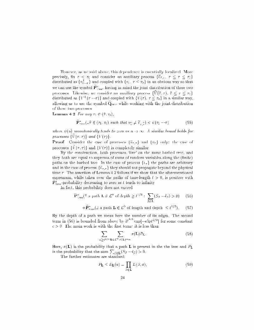
However, as we said above, this dependence is essentially localized. More
precisely, �x �� < �
0
and consider an auxiliary process fev
�� ;�
, �� � � � �
0
g
distributed as fv
+
����
g and coupled with fv
�
, � � �
0
g in an obvious way so that
we can use the symbol
b
P
�
tree
; having in mind the joint distribution of these two
processes. Likewise, we consider an auxiliary process f
e
V (�� ; � ), �� � � � �
0
g
distributed as fV
+
(� � �� )g and coupled with fV (� ), � � �
0
g in a similar way,
allowing us to use the symbol
e
Q
tree
while working with the joint distribution
of these two processes.
Lemma 4.2 For any �
1
2 (�� ; �
0
),
b
P
�
tree
(9b� 2 (�
1
; �
0
) such that v
b�
6= ev
�� ;b�
) < (�
1
� �� ) (55)
where (u) monotonically tends to zero as u!1. A similar bound holds for
processes f
e
V (�� ; � )g and fV (� )g:
Proof. Consider the case of processes fev
�� ;�
g and fv
�
g only: the case of
processes f
e
V (�� ; � )g and fV (� )g is completely similar.
By the construction, both processes `live' on the same barbed tree, and
they both are equal to suprema of sums of random variables along the (�nite)
paths on the barbed tree. In the case of process fv
�
g the paths are arbitrary
and in the case of process fev
��;�
g they should not propagate beyond the physical
time �� . The assertion of Lemma 4.2 follows if we show that the aforementioned
supremum, while taken over the paths of time-length t > 0; is positive with
b
P
�
tree
-probability decreasing to zero as t tends to in�nity.
In fact, this probability does not exceed
b
P
�
tree
(9 a path L 2 L
0
of depth � t
1=3
:
X
�2L
(S
�
� l
�
) > 0) (56)
+
b
P
�
tree
(9 a path L 2 L
0
of length and depth � t
1=3
): (57)
By the depth of a path we mean here the number of its edges. The second
term in (56) is bounded from above by 3
t
1=3
exp[�c�pt
2=3
] for some constant
c > 0. The main work is with the �rst term: it is less than
X
n�t
1=3
X
L2L
0
:d(L)=n
�(L)P
L
: (58)
Here, �(L) is the probability that a path L is present in the the tree and P
L
is the probability that the sum
P
�2L
(S
�
� l
�
) > 0:
The further estimates are standard:
P
L
� E
L
(a) =
Y
�2L
E(�; a); (59)
24

where E
L
(a) is the expectation value of exp[a
P
�2L
(S
�
� l
�
)] and E(�; a) is
the expectation value of exp[a(S
�
� l
�
)]: The last bound holds for any a > 0:
In view of (31) a straightforward calculation leads to
the RHS of (58) �
X
n�t
1=3
((1 + p) inf
a>0
�
(� + a)
Ee
as
)
n
: (60)
Under conditions (6) the series (60) converges. This leads to the assertion of
Lemma 4.2.
Lemma 4.2 allows us to �nish quickly the proof of Theorem 2. In fact,
let f : D ! R
1
be a continuous bounded function which is measurable with
respect to the �-algebra D(�
1
; �
0
): Fix an arbitrary � > 0. By using Lemma4.2,
we can choose �� < �
1
so that the di�erence
jE
P
f �E
e
P(�� )
f j < �; (61)
and a similar bound holds for the expectations with respect to the measures
Q and
e
Q(�� ): Here
e
P(�� ) and
e
Q(�� ) are the distributions of processes fev
�� ;�
g
and f
e
V (�� ; � )g; respectively. Then, keeping �� �xed, we perform the limiting
procedure ( 15.) for processes fev
�� ;�
g obtaining that
limE
e
P(��)
f = E
e
Q(�� )
f : (62)
To prove (62), we just need to repeat the proof of Theorem 4. Since � in (61)
is arbitrary, we get from (61) the relation
limE
P
f = E
Q
f : (63)
5 The travelling wave bound
The proof of Theorem 5 is based on the McKean formula (see
17
) for the
solution u(t;x) of the Cauchy problem equation (25), with initial date �(x):
u(� ;x) = Q
tree
(Y
�
< x); (64)
where Y
�
, � > 0, is a random process over the probability space (T; T ;Q
tree
)
(with the additional equipment by Wiener trajectories S
e
). Formally,
Y
�
= max
L(0;�)
X
e
(0;�)
�
�
S
e
(�g
e
)
�
: (65)
As follows from (47), with probability one, Y
�
� V
+
�
for all � � 0. Thus,
the bound
u(� ;x) � Q
+
(V
+
�
< x) (66)
holds for all x 2 R and � � 0. Using Proposition 2.3 completes the proof.
25

References
1. A.A. Borovkov, Convergence of the distributions of functionals of se-
quences and processes given on the entire axis. In: Proceedings of Steklov
Mathematical Institute, The USSR Academy of Sciences, vol. 128, 41{
65, (1972).
2. A.A. Borovkov, Asymptotical Methods in Queueing Theory. (Springer-
Verlag, Berlin, 1980)
3. F. Baccelli, F.I. Karpelevich, M.Ya. Kelbert, A.A. Pukhalskii, A.N. Ry-
bko and Yu.M. Suhov, Mean-�eld limit for a class of queueing networks.
J. Stat. Phys., 66, 803{825 (1992).
4. F. Baccelli, A. Makowski, Queueing models for systems with synchro-
nization constraints. Proceedings IEEE, 77, 138{161 (1989).
5. B. Chauvin and B. Rouault, KPP equation and supercritical branching
Brownian motion in the subcritical speed area. Application to spatial
trees. Prob. Theory Rel. Fields, 80, 299{314 (1988).
6. B. Chauvin, B. Rouault and A. Wakolbinger, Growing conditioned trees.
Stoch. Proc. Appl., 39, 117{130 (1991).
7. N.G. Du�eld, Local mean-�eld Markov processes: an application to mes-
sage switching networks. Prob. Theory Rel. Fields, 93, 485{505 (1992).
8. N.G. Du�eld, M.Ya. Kelbert and Yu.M. Suhov, A branching di�usion
approximation for a class of queueing networks. In: Stochastic Analysis
and Applications (I.M. Davies, A. Truman and K.D. Elworthy, Eds.)
pp201{220 (World Scienti�c, Singapore, 1996).
9. F.M. Dekking and B. Host, Limit distributions for minimal displacement
of branching random walk. Prob. Theory Rel. Fields, 90, 403{426 (1991)
10. M.I. Freidlin, Limit theorems for large deviations and reaction-di�usion
equations. Ann. Prob., 13, 639{675 (1985).
11. F.I. Karpelevich, M.Ya. Kelbert and Yu.M. Suhov, Higher-order Lindley
equations. Stoch. Proc. Appl., 53, 65{96 (1994).
12. F.I. Karpelevich, M.Ya. Kelbert and Yu.M. Suhov, The branching di�u-
sion, stochastic equations and travelling wave solutions to the equation
of Kolmogorov{Petrovskii{Piskunov. In: Cellular Automata and Coop-
erative Behaviour (N. Boccara, R. Goles, S. Martinez and P. Ricco, Eds.)
pp343{366 (Kluwer, Dordrecht, 1993).
13. F.I. Karpelevich, M.Ya. Kelbert and Yu.M. Suhov, Stochastic equations
on random trees. In: Cellular Automata and Cooperative Behaviour (N.
Boccara, R. Goles, S. Martinez and P. Ricco, Eds.) pp323{342 (Kluwer,
Dordrecht, 1993).
14. M.Ya. Kelbert and Yu.M. Suhov, Mathematical theory of queueing net-
26

works. Journ. of Soviet Mathematics, 50, 1527{1600 (1990).
15. M.Ya. Kelbert and Yu.M. Suhov, The Markov branching random
walk and system of reaction di�usion (Kolmogorov-Petrovskii- Piskunov)
equations. Commun. Math. Phys., 167, 607{634 (1995).
16. A. Kolmogorov, I. Petrovskii and N. Piscounov,
�
Etude de l'�equation de la
di�usion avec croissance de la quantit�e de la mati�ere et son application �a
un probl�eme biologique. Bull. Math. Moscow University, 1, 1{25 (1937)
17. H.P. McKean, Applications of Brownian motion to the equation of Kol-
mogorov - Petrovskii - Piscounov. Comm. Pure Appl. Math., 28, 323{
331 (1975).
27