Diffusion Tensor Imaging Analysis Guide

Dartmouth College, Gazzaniga Laboratory

Adam C. Riggall, Karl Doron & Megan S. Steven, PhD

Created: 9-25-06

1

Table of Contents

Table of Contents 1 Chapter 1: An Introduction to Linux 2

Intro to the Command Line 2 Command Summary 6

Chapter 2: Acquiring Data From the Scanner Inbox 7 Accessing the Scanner Inbox 7 Converting to NIFTI 7 Data Organization 8

Chapter 3: Analyzing DTI Data with FSL 10 Using the Graphical Interface for Processing 11 Using the Command Line Interface for Processing 15 Automation 16

Chapter 4: Probabilistic Tractography Analysis with FSL 17 Path Distribution Estimation 17 Connectivity-based Seed Classification 19 Quantitative Results 22 Combining Individuals into a Group 23 Automation 24

Chapter 5: FA Regression Analysis with TBSS and SPM 25 Using TBSS for Registration 25 Using SPM for Regression Analysis 26

Chapter 6: Tractography with DTIStudio 30 Chapter 7: Image Viewing & Manipulation 34

Using FSLView 34 Drawing Seed Masks in FSLView 35 Using MRIcro 36 Drawing Seed Masks in MRIcro 36 Saving Images 37 Creating Seed Masks with WFUPickAtlas 37

Chapter 8: Remote Access 39 Using SSH for Command Line Remote Access 39 Using VNC for Graphical Remote Access 39 Accessing AFS Remotely 40

2

Chapter 1: An Introduction to Linux Before we can begin analyzing neuroimaging data we need to become familiar with the platform on which we will be working. Most of the data analysis is done using Linux machines. What is Linux? Linux is just another operating system, similar to Microsoft Windows or Mac OS X. However, instead of being developed by any particular company or individual, Linux is a collaborative effort by thousands of people worldwide who share their code in an attempt to make the best operating system possible. It is one of the original open source projects, a model which has since been used in countless projects to produce incredible results. Why do we use Linux? There are a variety of reasons. It’s incredibly stable and rarely, if ever, crashes. It’s very secure. It works extremely well in a networked environment, allowing for easy network file storage and remote access. It’s also very easy to administer remotely, allowing for the department system administrator to keep all the systems up to date. Finally, it’s free. Why to waste extra money on a operating system when you don’t have too? There are a few notes to point out about Linux and the particular set up we have in the neuroimaging lab. Linux has a very strong user permissions system. Anyone using the system must login with a specific username and password. Additionally, all files have permissions associated with them, restricting the ways in which a user can interact with each file. In general a user has full permission to do anything to all the files contained in their home directory, and only permission to read any system wide files, and no permissions to files contained in other users home directories. Additionally, Linux is a true multi-user operating system, allowing many users to share a system at the same time. This has important implications when multiple users are trying to perform extremely computer intensive tasks, as each steals computing time from the others, slowing down the processing time for everyone. However, this only becomes important when working with data remotely, and should never be a problem while working on the machines in the neuroimaging lab. In the lab, all of our data is stored remotely on a network server known as AFS. When you log in to a computer it connects to the AFS server and treats the remote data as if it were a local hard drive. Due to the extremely high speed connection with the server, this process is completely transparent, with most files loading immediately, as if they were stored locally. This network storage provides several benefits. Firstly, it provides data security, as it is often backed up and won’t be lost due to local hardware malfunctions. Secondly, it allows us access to our data from any location at any time. Additionally, it allows multiple people and multiple systems to be working on our data simultaneously. This needs to be done carefully, as two users working on exactly the same files are likely to corrupt the data and cause other strange, hard to track down problems. By being careful to segregate what each person is working on, these troubles should be easily avoided.

Intro to the Command Line While modern Linux machines have a full graphical desktop similar to Windows or OS X, much of our time will be spent avoiding it, instead using the Command Line Interface (CLI) to do most of our work. We do this because the command line allows us to interact with our data much more efficiently. Most people are initially dismayed by the thought of using the command line, thinking of it as antique and out-dated, however you will find that it is extremely powerful, allowing you to complete tasks in seconds with a simple one line command which would have taken minutes of tedious pointing and clicking in the graphic interface. It also provides us with a direct link to powerful scripting features which will prove invaluable in speeding up work flow and insuring that every step is executed in exactly the same manner each time an analysis is run. In order to access the command line, simply right click on the desktop and select “Open Terminal”. This will open up a terminal which will contain a simple command prompt, as seen here: [meg@dbic-lab_x86-64_04 ~]$

This prompt provides us with several pieces of information. Firstly, it tells us who we are logged in as, in this case the user “meg”. Secondly, it tells us the specific machine we are logged into, “dbic-lab_x86-64_04”. Finally, it tells us the current directory that we are in, in this case “~”, a Linux shortcut for our home directly. To find out the full

3

path of the directory we are currently in, we can use the pwd, to show us our present working directory: [meg@dbic-lab_x86-64_04 ~]$ pwd /afs/dbic.dartmouth.edu/usr/gazzaniga/meg

This command is useful when you have moved around a lot and are not sure exactly which directory you are in anymore. To find out what is contained within the directory we are currently in, we can use the list command ls: [meg@dbic-lab_x86-64_04 ~]$ ls 01-splenium-parcellation Desktop F5 M12 M8 spm2 02-full-cc-parcellation F1 F6 M13 M9 study 03-rvfa-fa-regression F10 F7 M2 avg152T1.nii.gz tal 04-grooved-pegboard-fa-regression F11 F8 M3 bvals 05-farah-fa-regression F12 F9 M4 bvecs

This list shows all of the files and directories that are contained within our home directory. It is colored coded to give you hints as to what each listing means. Anything in blue is directory. Other colors may be used to indicate other types of files. In order to change to a new directory, we can use cd, the change directory command, and any of the directories we could move to. [meg@dbic-lab_x86-64_04 ~]$ cd study [meg@dbic-lab_x86-64_04 study]$

Notice how the prompt changed to indicate the current directory we are now in. There are several shortcuts you should know for changing directories. If you type cd without anything following it, this will automatically take you to your home directory. If you type cd followed by two dots (cd ..), you will return to the directory one level above the one you are currently in. Additionally, you can chain together directories, to allow you to move through several levels in a single command. The following example takes us up two directories, into the ‘study’ directory, into the ‘s01’ directory. [meg@dbic-lab_x86-64_04 results]$ pwd /afs/dbic.dartmouth.edu/usr/gazzaniga/meg/1-splenium-parcellation/results [meg@dbic-lab_x86-64_04 results]$ cd ../../study/s01 [meg@dbic-lab_x86-64_04 s01]$ pwd /afs/dbic.dartmouth.edu/usr/gazzaniga/meg/study/s01

To create a new directory, we can use the make directory command, mkdir: [meg@dbic-lab_x86-64_04 results]$ ls group1.feat group2.feat stats.txt [meg@dbic-lab_x86-64_04 results]$ mkdir combined [meg@dbic-lab_x86-64_04 results]$ ls combined group1.feat group2.feat stats.txt

If you would like to delete a directory, it must be empty, and then you can use the remove directory command, rmdir: [meg@dbic-lab_x86-64_04 results]$ rmdir combined [meg@dbic-lab_x86-64_04 results]$ ls group1.feat group2.feat stats.txt Dealing with files is equally simple. In order to move a file or a directory, we use mv: [meg@dbic-lab_x86-64_04 results]$ ls group1.feat group2.feat stats.txt [meg@dbic-lab_x86-64_04 results]$ mv stats.txt group1.feat/ Above we moved a file into a directory. We can also use mv to rename a file, as seen below: [meg@dbic-lab_x86-64_04 results]$ ls group1.feat group2.feat stats.txt [meg@dbic-lab_x86-64_04 results]$ mv stats.txt newstats.txt [meg@dbic-lab_x86-64_04 results]$ ls

4

group1.feat group2.feat newstats.txt

If we wish to copy a file, just like the move command, we can copy with cp: [meg@dbic-lab_x86-64_04 results]$ ls group1.feat group2.feat stats.txt [meg@dbic-lab_x86-64_04 results]$ cp stats.txt newstats.txt [meg@dbic-lab_x86-64_04 results]$ ls group1.feat group2.feat newstats.txt stats.txt

Now for a word of caution about mv and cp before we continue. They will automatically overwrite files with the same name as the target without any warning. Be sure that a file doesn’t already exist with the same name at the destination before moving or copying or you will end up overwriting something which you didn’t intend to, and possibly permanently losing something important. The final basic command that you should know is how to delete a file, using the remove command rm: [meg@dbic-lab_x86-64_04 results]$ ls group1.feat group2.feat stats.txt [meg@dbic-lab_x86-64_04 results]$ rm stats.txt [meg@dbic-lab_x86-64_04 results]$ ls group1.feat group2.feat

Again, a word of caution. The rm command will delete all files passed to it, without any question. We need to make sure we really don’t need a file before removing it. Now for a couple of tricks which will greatly speed up our interactions with the command line. The first is called tab completion. If we are attempting to move a file with a rather long name, we don’t need to type out the whole name of the file. We can simply type out the first few letters of the filename and then hit the Tab key. It should automatically complete the filename for us. If it does not, that means that we didn’t provide enough information to single out the file. If we hit the Tab key once more, it will show all those filenames which could be completed with the few letters we gave it. By examining this list we should be able to determine how many more characters we need to type for disambiguation. For example: [meg@dbic-lab_x86-64_04 stats]$ ls newstats1.txt newstats2.txt oldstats1.txt olddata.txt [meg@dbic-lab_x86-64_04 stats]$ mv old{Tab} oldstats.txt olddata.txt [meg@dbic-lab_x86-64_04 stats]$ mv oldd{Tab} [meg@dbic-lab_x86-64_04 stats]$ mv olddata.txt In the above example, ‘old’ wasn’t enough to provide unambiguous information about which file we were talking about, but with the added ‘d’, to make ‘oldd’, tab completion successfully finished the filename for us. The second trick for speeding up command line interactions is extremely powerful. It is the use of wild cards Just like wild cards in poker, command line wild cards are symbols that when used on the command line are interpreted to mean any character. This allows us to interact with a large number of files which all share a common naming element in a single command. Say for example that we have a directory which contains a hundred files named ‘a000.txt’, ‘a001.txt’ and so forth, as well as a hundred other files name ‘b000.txt’, ‘b001.txt’, etc. If we wanted to move all of the files beginning with an ‘a’ to the parent directory, we could type 100 individual mv commands, one for each file. This would incredibly tedious however, and wild cards provide a much quicker solution. By using the ‘*’ wild card, we can move all the ‘a’ files in a single command: [meg@dbic-lab_x86-64_04 files]$ mv a* .. The wild card tells the system to move all files that begin with ‘a’ to the directory above us. Using wild cards you can achieve a wide degree of flexibility in how you move files around. If we wanted only those files which were a multiple count of 10 we could do so easily, this time with a leading wild card: [meg@dbic-lab_x86-64_04 files]$ mv *0.txt ..

5

Wild cards are extremely handy when moving around a lot of files. They can also be dangerous if used incorrectly, causing us to accidentally move or remove files that weren’t intended. An easy way to verify that we are only getting the files we want with a wild card command is to first use the wild card string in a ls command. For example if we want to move the multiples of 10 that start with ‘a’ we could test our string: [meg@dbic-lab_x86-64_04 files]$ ls a*0.txt a0000.txt a0020.txt a0040.txt a0060.txt a0080.txt a0010.txt a0030.txt a0050.txt a0070.txt a0090.txt

Our listing shows only the files that we actually want to move, so we can safely execute the move command using that wild card string. With these few common commands, and a few more we will pick up on the way, we can quickly and efficiently manipulate all of our data, without ever needing to take our hands off the keyboard. As a final note we will conclude this chapter with a quick discussion about the standard format of a command line call. A typical call consist of the name of the command, such as ls for list, followed by any options we want to pass to the program, and finally any arguments we are passing. Options are typically things which will change the operation of the actual command, and arguments are things, usually other files or directories, on which the command will be acting. Let’s look at the following example: meg@dbic-lab_x86-64_04 files]$ ls -l a*0.txt -rw-r--r-- 1 meg users 1251 Sep 18 21:07 a0000.txt -rw-r--r-- 1 meg users 48 Sep 18 21:07 a0010.txt -rw-r--r-- 1 meg users 48 Sep 18 21:07 a0020.txt -rw-r--r-- 1 meg users 1251 Sep 18 21:07 a0030.txt -rw-r--r-- 1 meg users 0 Sep 18 21:05 a0040.txt -rw-r--r-- 1 meg users 0 Sep 18 21:05 a0050.txt -rw-r--r-- 1 meg users 697 Sep 18 21:07 a0060.txt -rw-r--r-- 1 meg users 1575 Sep 18 21:07 a0070.txt -rw-r--r-- 1 meg users 1575 Sep 18 21:07 a0080.txt -rw-r--r-- 1 meg users 697 Sep 18 21:07 a0090.txt

Here we have our command name, ls, followed by one option, -l, and a wild card argument, which we know from above expands out to be every file which starts with ‘a’ and ends with ‘0.txt’. The -l option tells the list command that we would like to see a long, more detailed listing of the specific files. This includes information about the permissions of the file, the owner, the size, and when it was last modified. In order to find out all of the options available for a given command, you can use yet another command, the man command, to open up a manual containing more information than you could even want to know about a command. For example, the following will show all the information contained in the ls manual: meg@dbic-lab_x86-64_04 files]$ man ls Man pages are typically extremely detailed, and will usually provide examples of how each one can be used. They often also provide you with links to other more detailed resources and examples, as well as related programs which may also be of interest. Every standard Linux command follows the same format (command, options, argument), and almost every standard command has a very detailed man page. Unfortunately for us, the developers of FSL did not follow this standard, and in fact didn’t seem to follow any standard. Sometimes command line FSL programs do follow the standard (command, options, arguments), but many other times they reverse the position of the arguments and options, causing the program to fail if called in the standard manner. We’ll try to note as we go along which ones are irregular, but just in case, if we ever have problems with FSL programs, we can simply type the name of the command, with no arguments or options, and it will print out instructions for the correct usage.

6

Command Summary

Command Function Common Options pwd List present working directory

ls List contents of the current directory -l Detailed listing of contents

cd Change directory

mkdir Make a new directory rmdir Remove an empty directory

mv Move a file or directory

cp Copy a file or directory -r Copy all contents of a directory recursively

rm Remove a file (or directory with -f) -f Remove a directory and everything in it

7

Chapter 2: Acquiring Data From the Scanner Inbox After we have acquired imaging data for a subject on the scanner, that data is pushed into the scanner inbox, where the data is stored until we wish to access it. When it is time to start analyzing the data, there are several steps we must take to move the data out of the inbox and into our AFS home directory. These include insuring that the data has been successfully pushed off the scanner, converting it to more useful formats, and storing it in a logical manner in our home directory.

Accessing the Scanner Inbox The first step is to insure that the data has successfully moved from the scanner’s local storage into the inbox. To do this we must remotely access the inbox system, rolando.cns. To do this, we use the secure shell, ssh. This allows us to login as a remote user, as in below. When we issue the ssh command, passing it the server we want to connect to, it will ask us to enter our password. For security purposes, no characters will be used to represent the password on the screen as we type, it remains blank. Once we have successfully logged in, notice how the server name in the prompt changes to illustrate that we are now working on a different system. [meg@dbic-lab_x86-64_04 ~]$ ssh rolando.cns meg@rolando.cns's password: Last login: Tue Aug 29 11:18:03 2006 from dbic-lab_x86-64_04.kiewit.dartmouth.edu [meg@rolando ~] >

The next step we must take is to change into the inbox directory, which can be seen below. The studyname should be whatever name was used to define the study while performing the scan. While in the study directory we can get a listing of all the subjects that have been scanned and successfully moved to the inbox. [meg@rolando ~] > cd /inbox/INTERA/studyname [meg@rolando studyname] > ls 02jul06db 02jul06dm 02jul06ln 02jul06wd 05jul06fa

The data in the inbox is stored in Philips native imaging file format, .par/.rec. Unfortunately for us, the software which we will be using does not read this format, so we must convert the data to a more commonly used format, Analyze, before we can start to process it. To do this we will be using a Matlab script which does the conversion and copies the data to our home directory in one step. First we need to start Matlab, by calling the matlab command. Once Matlab starts, we will now be working inside Matlab, indicated by the simple >> prompt. The conversion script is called par_convert and takes the subject identifier as a first argument, and the location where we would like the data copied as a second argument: [meg@rolando studyname] > matlab (Matlab startup text removed) >> par_convert('02jul06db','/afs/dbic.dartmouth.edu/usr/gazzaniga/meg/02jul06db'); (Matlab script text removed)

This step must be repeated for each subject we wish to convert and copy to our home directory. Once this is done, we simply exit out of matlab, and then exit out of our remote session to return to working where we started. >> exit [meg@rolando studyname] > exit [meg@dbic-lab_x86-64_04 ~]$

Converting to NIFTI We have now successfully converted the data to a more usable format and copied it into our home directory. Sadly, the format which the above script outputs, Analyze, is quite inefficient in terms of disk usage. All of the files are quite large and would quickly fill up our home directory. To help improve our disk usage, we convert the files one more time to a different file format, known as NIFTI. Specifically, we use a compressed version of NIFTI, which allows a file which used to be over 20mb in Analyze to only take up 700kb in the compressed NIFTI format, a more than 90% reduction. All this without losing any information.

8

To take care of this conversion step we have created a script called analyze2nifti which takes a directory as an argument and proceeds to recurse through the directory, converting all the analyze files it finds inside to the NIFTI format. However, before we see how to use the script, we should understand what it is actually doing. To take care of the actual conversion we are using a program called avwchfiletype, provided with FSL. This program takes as an argument the type of file we want to convert to, and the file to convert. It automatically converts the file and renames it appropriately. [meg@dbic-lab_x86-64_04 ANATOMY]$ ls coplanar.hdr coplanar.img mprage.hdr mprage.img [meg@dbic-lab_x86-64_04 ANATOMY]$ avwchfiletype NIFTI_GZ coplanar.hdr [meg@dbic-lab_x86-64_04 ANATOMY]$ avwchfiletype NIFTI_GZ mprage.hdr [meg@dbic-lab_x86-64_04 ANATOMY]$ ls coplanar.nii.gz mprage.nii.gz

In order to process a large number of files without having to enter the avwchfiletype command repeatedly, we can use the analyze2nifti script. Given a directory this script will automatically convert all the Analyze files inside to NIFTI format. [meg@dbic-lab_x86-64_04 study]$ ls s01 s02 s03 s04 s05 s06 s07 s08 s09 s10 s11 s12 [meg@dbic-lab_x86-64_04 study]$ analyze2nifti s01 Found 247 analyze files to convert Would you like to convert these files (y/n)? y [##################################100%#####################################] 247/247 Done!

Data Organization

That is all for getting the data ready to be preprocessed and analyzed, but before we move on it is important to take a second to plan out how we are going to store all of our data in an organized manner. During analysis we will be producing a great number of files, and if we don’t have an organized file structure we are bound to lose files, or get things confused. One simple method to solving this problem is to create a single directory within our home directory for each individual study, ideally naming them with the date the study started to help organized further. Lets pretend we have two studies in our home directory. A listing of home would look like this: meg@dbic-lab_x86-64_04]$ ls ~ 20060812-love-dti-study 20060822-monkey-ac-study bin matlab Within each study directory, we can create several directories to hold various portions our analysis. We should start out with a ‘subjects’ directory, which will contain the individual data for each subject. We also want a ‘group’ directory, for when we group the individuals as well as a ‘results’ directory to hold any results we produce. It may also be necessary to have a ‘masks’ directory, if we will be using mask images, or some other study appropriate data, such a behavioral data. Finally, as we become proficient with scripting, it is often extremely handy to have a specific ‘scripts’ directory within each study we are working on. After moving our individual subjects data over from the scanner inbox, we will want to move it into the subjects directory, within the specific study directory. It is also probably a good idea at this time to rename the directory to something shorter and easier to type, while making sure to document exactly how subjects are renamed. Common new subjects names would be f01,f02,...,m01,m02,... for females and males, or perhaps c01,c02,...,x01,x02,... for control and experimental subjects. Doing this makes it easier to type as well and easier to work with while scripting. We can visualize our directory layout using the tree command. A single study should look something like the following: [meg@dbic-lab_x86-64_04 home]$ tree 20060812-love-dti-study/ 20060812-love-dti-study/ |-- behavioral |-- group |-- results `-- subjects

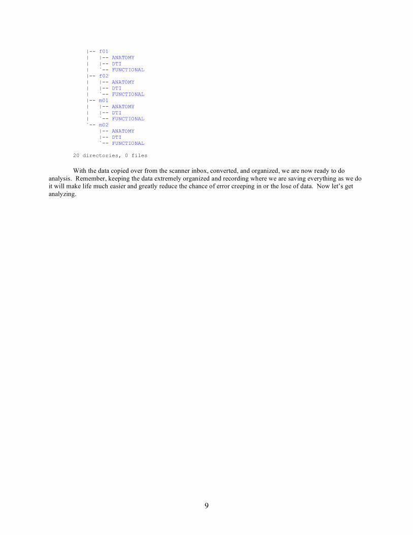
9

|-- f01 | |-- ANATOMY | |-- DTI | `-- FUNCTIONAL |-- f02 | |-- ANATOMY | |-- DTI | `-- FUNCTIONAL |-- m01 | |-- ANATOMY | |-- DTI | `-- FUNCTIONAL `-- m02 |-- ANATOMY |-- DTI `-- FUNCTIONAL 20 directories, 0 files

With the data copied over from the scanner inbox, converted, and organized, we are now ready to do analysis. Remember, keeping the data extremely organized and recording where we are saving everything as we do it will make life much easier and greatly reduce the chance of error creeping in or the lose of data. Now let’s get analyzing.

10

Chapter 3: Analyzing DTI Data with FSL

The FMRIB’s Diffusion Toolbox (FDT), which is included in the FMRIB’s Software Library (FSL) distribution provides us with an excellent set of tools for analyzing diffusion-weighted imaging data. An intuitive graphical interface makes jumping in and using it easy, while a full set of command line programs allows for powerful scripting and automation. We’ll go through using both methods for analysis, but before we begin there are several preprocessing steps which must be done for each subject to get the data in a format that will work with FSL. To begin lets start in the ‘DTI’ directory of a subject. For a normal subject with only one DTI scan this directory will contain 34 files, named ‘dti1_0001.nii.gz’ through ‘dti1_0034.nii.gz’. The first image, ‘dti1_0001.nii.gz’ is our b0 image, the image with no diffusion gradient active. Images 2 through 33 are for each of the various gradient directions. The last image is a trace image which is created automatically by the scanner and which we don’t need for the analysis. In order to get the data ready for use with FSL we have to rename the trace image, create a copy of the b0 image, and convert the data from individual 3d files into a single 4d file. This can all be accomplished with a few simple commands on the command line: [meg@dbic-lab_x86-64_04 DTI]$ pwd /afs/dbic.dartmouth.edu/usr/gazzaniga/meg/study/s01/DTI [meg@dbic-lab_x86-64_04 DTI]$ ls dti1_0001.nii.gz dti1_0008.nii.gz dti1_0015.nii.gz dti1_0022.nii.gz dti1_0029.nii.gz dti1_0002.nii.gz dti1_0009.nii.gz dti1_0016.nii.gz dti1_0023.nii.gz dti1_0030.nii.gz dti1_0003.nii.gz dti1_0010.nii.gz dti1_0017.nii.gz dti1_0024.nii.gz dti1_0031.nii.gz dti1_0004.nii.gz dti1_0011.nii.gz dti1_0018.nii.gz dti1_0025.nii.gz dti1_0032.nii.gz dti1_0005.nii.gz dti1_0012.nii.gz dti1_0019.nii.gz dti1_0026.nii.gz dti1_0033.nii.gz dti1_0006.nii.gz dti1_0013.nii.gz dti1_0020.nii.gz dti1_0027.nii.gz dti1_0034.nii.gz dti1_0007.nii.gz dti1_0014.nii.gz dti1_0021.nii.gz dti1_0028.nii.gz [meg@dbic-lab_x86-64_04 DTI]$ mv dti1_0034.nii.gz trace.nii.gz [meg@dbic-lab_x86-64_04 DTI]$ cp dti1_0001.nii.gz nodif.nii.gz [meg@dbic-lab_x86-64_04 DTI]$ avwmerge dti1 dti1_* All of the above commands should be familiar, except for the final line. The avwmerge command takes a series of 3d volumes and converts them into a new single 4d volume, while leaving the old 3d files in place. The first argument is the name of the new 4d file, and the remaining arguments are all the individual 3d files. Above we have used a wild card to automatically include all the diffusion-weighted files. A few final steps are needed to get the data ready for analysis. First we need to make a mask of just the brain area of the b0 image, which can be done using FSL’s brain extraction tool, bet. The options given at the end are those which have been found to provide the best results for our specific scanner. Finally we need to include the files which tell us the gradient directions and values. To insure that we are always using the correct files, it is easiest to keep a master copy permanently located in the home directory. We can then link to them, using the ln command, as shown below. Linking essentially creates a copy of the file, but without taking up any space. This has the added benefit that if we discover that a change needs to be made to either of these files, it will be immediately updated in all the places it has been linked from. [meg@dbic-lab_x86-64_04 DTI]$ bet nodif nodif_brain -f .3 -m [meg@dbic-lab_x86-64_04 DTI]$ ln -s ~/bvecs [meg@dbic-lab_x86-64_04 DTI]$ ln -s ~/bvals At the end of this whole preprocessing step we should have a directory which contains the following files: [meg@dbic-lab_x86-64_04 DTI]$ ls bvals dti1_0008.nii.gz dti1_0018.nii.gz dti1_0028.nii.gz bvecs dti1_0009.nii.gz dti1_0019.nii.gz dti1_0029.nii.gz dti1.nii.gz dti1_0010.nii.gz dti1_0020.nii.gz dti1_0030.nii.gz dti1_0001.nii.gz dti1_0011.nii.gz dti1_0021.nii.gz dti1_0031.nii.gz dti1_0002.nii.gz dti1_0012.nii.gz dti1_0022.nii.gz dti1_0032.nii.gz dti1_0003.nii.gz dti1_0013.nii.gz dti1_0023.nii.gz dti1_0033.nii.gz dti1_0004.nii.gz dti1_0014.nii.gz dti1_0024.nii.gz nodif.nii.gz dti1_0005.nii.gz dti1_0015.nii.gz dti1_0025.nii.gz nodif_brain.nii.gz dti1_0006.nii.gz dti1_0016.nii.gz dti1_0026.nii.gz nodif_brain_mask.nii.gz dti1_0007.nii.gz dti1_0017.nii.gz dti1_0027.nii.gz trace.nii.gz

11

Using the Graphical Interface for Processing Now that the data has been set up in the ‘DTI’ directory in a way that will work well with FSL, we can begin processing the data. The first step is to launch FDT, which can be done with a command line call of Fdt, or by click on ‘FDT Diffusion’ in the main FSL window. This will launch FDT and bring up the main window. The first processing step we need to take is to correct for eddy currents, which occur due to the changing gradient field directions, and head motion. Both of these are accomplished in one step using the ‘Eddy current correction’ step of FDT. To begin, select this option from the top left pull down box. The screen should resemble the image below. For the ‘Diffusion weighted data’ we will want to select the 4d file we created above, called ‘dti1.nii.gz’. For the ‘Corrected output data’ we will use ‘data.nii.gz’, a name which will make future steps simpler. We can leave the reference volume at its default value of ‘0’, because our zeroth image (when counting from 0) is our b0 image. Finally all we have to do is click ‘Go’. This step takes approximately 30-45 minutes per subject.

Following eddy current correction we can now use DTIFit to fit tensors to the data and determine a variety of values include the fractional anisotropy at each voxel as well as the principle diffusion direction. To perform this step we simply select ‘DTIFit Reconstruct diffusion tensors’ from the upper left drop down menu and then select the individual subjects DTI directory and hit ‘Go’. This step is fairly quick, taking only a couple of minutes to fully complete.

We have finally produced some results worth looking at in this previous step. In order to view them we can use FSLView, which can be launched from the command line by typing fslview or through the main FSL window. NB: fsl only runs on the Dell computers in the neuroimaging lab at this time (not the Suns). After FSLView has loaded we want to go ahead and load an image. To do this we select ‘Open’ from the file menu and chose the ‘data_FA.nii.gz’ volume which was just created by DTIFit. This shows us the fractional anisotropy (FA) value at each voxel. Next we can examine the principle diffusion direction at each voxel. To do this we start by selecting ‘Add’ from the ‘File’ menu and choosing the ‘data_V1.nii.gz’ volume. When the volume loads, it will most likely initially look like random noise. In order to fix this, we click on the blue circle with an ‘I’ inscribed, which can be found just left of the midline, near the bottom of the FSLView window. This will bring up the ‘Overlay Information Dialog’ as seen below:

12

Under the ‘DTI display options section’, we change the ‘Display as’ drop down menu to ‘RGB’ and change the ‘Modulation’ drop down menu to ‘data_FA’. This should change the display to look something like below.

Here we can see the principle diffusion direction as represented by color. Red indicates that the fibers at that voxel are running in the left-right direction, blue indicates the inferior-superior direction (down-up), and green means they are running in the anterior-posterior direction (front-back).

13

The next step in processing is one of the simplest to start while being one of the most time-consuming to run. In order to run probabilistic tractography on our data, we first need to prepare it by running a program call BEDPOST on it. This program builds sampling distributions on the diffusion parameters at each voxel, which are used for the tractography. To perform this step we simply select ‘BEDPOST Estimation of diffusion parameters’ from the upper left drop down menu and then select the individual subjects ‘DTI’ directory and hit ‘Go’. This step takes approximately 8-10 hours per subject and in the end will produce a new folder called ‘DTI.bedpost’ in the subjects directory which we will be using in the future when we do tractography.

The final processing step we need to perform before we can get into tractography involves registering the diffusion weighted images to our high resolution structural image and to a standard space image. The registration to structural space requires a skull stripped high-res image. If we don’t have one of those, we can create one using bet, as shown below, using the ‘mprage.nii.gz’ found in the subjects ‘ANATOMY’ directory. [meg@dbic-lab_x86-64_04 ANATOMY]$ bet mprage mprage_brain –f .35 –g -.4

To perform the registration we select ‘Registration’ from the FDT upper left drop down menu. For the Bedpost directory we need to select the recently created ‘DTI.bedpost’. In order to do registration to structural space we need to activate the checkbox to the left of the ‘Main structural image’ section. This will allow us to select a structural image, which should be the skull stripped high-res image for the subject. We shouldn’t need to change anything for the standard space resolution section. By clicking ‘Go’ and waiting a few minutes we have generated transformations which will allow us to change any volume to any other volume’s space. NB: to transform between the diffusion and individual structural spaces you want 6DOF; between the structural and standard spaces you want 12DOF.

That finishes it for the processing steps required to analyze diffusion weighted images using the graphical interface. Skip ahead to the “Probabilistic Tractography with FSL” section to continue with the analysis, or read on to see how to do all of the above steps from the command line.

14

15

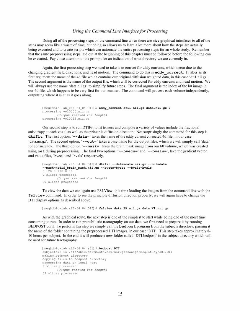
Using the Command Line Interface for Processing

Doing all of the processing steps on the command line when there are nice graphical interfaces to all of the steps may seem like a waste of time, but doing so allows us to learn a lot more about how the steps are actually being executed and to create scripts which can automate the entire processing steps for an whole study. Remember that the same preprocessing steps laid out at the beginning of this chapter must be followed before the following can be executed. Pay close attention to the prompt for an indication of what directory we are currently in. Again, the first processing step we need to take is to correct for eddy currents, which occur due to the changing gradient field directions, and head motion. The command to do this is eddy_correct. It takes as its first argument the name of the 4d file which contains our original diffusion weighted data, in this case ‘dti1.nii.gz’. The second argument is the name of the output file, which will be corrected for eddy currents and head motion. We will always use the name ‘data.nii.gz’ to simplify future steps. The final argument is the index of the b0 image in our 4d file, which happens to be very first for our scanner. The command will process each volume independently, outputting where it is at as it goes along. [meg@dbic-lab_x86-64_04 DTI]$ eddy_correct dti1.nii.gz data.nii.gz 0 processing vol0000.nii.gz (Output removed for length) processing vol0032.nii.gz

Our second step is to run DTIFit to fit tensors and compute a variety of values include the fractional anisotropy at each voxel as well as the principle diffusion direction. Not surprisingly the command for this step is dtifit. The first option, ‘--data=’ takes the name of the eddy current corrected 4d file, in our case ‘data.nii.gz’. The second option, ‘--out=’ takes a base name for the output files, which we will simply call ‘data’ for consistency. The third option ‘--mask=’ takes the brain mask image from our b0 volume, which was created using bet during preprocessing. The final two options, ‘--bvecs=’ and ‘--bvals=’, take the gradient vector and value files, ‘bvecs’ and ‘bvals’ respectively. [meg@dbic-lab_x86-64_04 DTI]$ dtifit --data=data.nii.gz --out=data --mask=nodif_brain_mask.nii.gz --bvecs=bvecs --bvals=bvals 0 128 0 128 0 70 0 slices processed (Output removed for length) 69 slices processed

To view the data we can again use FSLView, this time loading the images from the command line with the fslview command. In order to see the principle diffusion direction properly, we will again have to change the DTI display options as described above. [meg@dbic-lab_x86-64_04 DTI]$ fslview data_FA.nii.gz data_V1.nii.gz As with the graphical route, the next step is one of the simplest to start while being one of the most time consuming to run. In order to run probabilistic tractography on our data, we first need to prepare it by running BEDPOST on it. To perform this step we simply call the bedpost program from the subjects directory, passing it the name of the folder containing the preprocessed DTI images, in our case ‘DTI’. This step takes approximately 8-10 hours per subject. In the end it will produce a new folder called ‘DTI.bedpost’ in the subject directory which will be used for future tractography. [meg@dbic-lab_x86-64_04 s01]$ bedpost DTI subjectdir is /afs/dbic.dartmouth.edu/usr/gazzaniga/meg/study/s01/DTI making bedpost directory copying files to bedpost directory processing data on local host 1 slices processed (Output removed for length) 69 slices processed

16

The final step, registration from diffusion to standard and structural space, is the most complicated to perform on the command line, as it consists of a series of rather complicated command line calls. While this step is usually easier to do in the graphical interface, knowing what is going on underneath provides us with the flexibility to script the whole process start to finish. Within the ‘DTI.bedpost’ directory we create a new folder, ‘xfms’, to hold the transformation matrices, and then use flirt to register the images, and convert_xfm to create inverses and combinations of transformations. The options and arguments being passed should be easy to follow if we read through carefully. [meg@dbic-lab_x86-64_04 DTI.bedpost]$ mkdir xfms [meg@dbic-lab_x86-64_04 DTI.bedpost]$ flirt -in nodif_brain

-ref ../ANATOMY/mprage_brain.nii.gz -omat xfms/diff2str.mat -searchrx -90 90 -searchry -90 90 -searchrz -90 90 -dof 12 -cost mutualinfo

[meg@dbic-lab_x86-64_04 DTI.bedpost]$ convert_xfm -omat xfms/str2diff.mat -inverse xfms/diff2str.mat [meg@dbic-lab_x86-64_04 DTI.bedpost]$ flirt -in ../ANATOMY/mprage_brain.nii.gz

-ref /afs/dbic.dartmouth.edu/usr/pkg/fsl/etc/standard/avg152T1_brain -omat xfms/str2standard.mat -searchrx -90 90 -searchry -90 90 -searchrz -90 90 -dof 12 -cost corratio

[meg@dbic-lab_x86-64_04 DTI.bedpost]$ convert_xfm -omat xfms/standard2str.mat -inverse xfms/str2standard.mat

[meg@dbic-lab_x86-64_04 DTI.bedpost]$ convert_xfm -omat xfms/diff2standard.mat -concat xfms/str2standard.mat xfms/diff2str.mat

[meg@dbic-lab_x86-64_04 DTI.bedpost]$ convert_xfm -omat xfms/standard2diff.mat -inverse xfms/diff2standard.mat

Automation

In order to speed up analysis, now that we know all of the steps, we can use a script which implements these steps in sequence. Running doDTI from within a subject directory will automatically perform all of the preprocessing, analysis and registration steps, including running bedpost. This script uses default options, and expects the initial files ‘dti1_00*.nii.gz’ to be in a folder called ‘DTI’ in the subjects main directory, as well as a skull stripped high resolution anatomical image to be in the folder ‘ANATOMY’. Processing for a single subject will take approximately 10 hours. [meg@dbic-lab_x86-64_04 s01]$ doDTI Preprocessing data Correcting eddy currents Running DTIFit Running bedpost Registering diffusion to structural and standard space Done!

17

Chapter 4: Probabilistic Tractography Analysis with FSL

Rather than generating specific discrete tube-like pathways as other tractography applications often do, FSL’s implementation of tractography is probabilistic, creating a distribution of possible pathways, weighted by their likelihood. In order to do this, the analysis software, FDT’s ProbTrack, sends a given number of samples out from each seed voxel. These samples follow the principle diffusion direction of the underlying white matter, choosing a random path when presented with multiple choices. By looking at pathways which a large number of samples passed through we can get a good idea of the underlying pathways. This probabilistic method allows us to easier quantify the data and compare across individuals. ProbTrack provides two main methods for looking at our data. The first, path distribution estimation, maps out connections from a starting point. The second, connectivity based seed classification, allows us to quantify voxels in an specific area by the other areas in the brain they may be connected to. Before we can begin with this step of analysis, our data must have already been processed as described above in the DTI analysis chapter. Also, it is often times necessary to use masks to define the areas we are interested in. The Image Viewing and Manipulation chapter below describes several methods for creating masks.

Path Distribution Estimation The first ProbTrack method allows us to visual pathways as they traverse the brain. To begin with we need to launch FDT, which can be done with a command line call of Fdt, or by click on ‘FDT Diffusion’ in the main FSL window. This will launch FDT and bring up the main window. To do any sort of tractography we need to get to the FDT ProbTrack section, by selecting ‘ProbTrack Probabilistic tractography’ from the upper left drop-down menu. By default, the simplest tracking method, going from a single voxel is selected. This method would be useful if we had a very specific spot we wanted to track from. More commonly used is the second path distribution estimation method, using a seed mask. We’ll walk through the steps to perform this route below. To start we need to select ‘Seed mask’ from the second drop down menu.

Now that we are ready to use the seed mask method, we simply need to select a few directories and files. First we need to select the bedpost directory for the subject on which we will be working, which should be called ‘DTI.bedpost’ and found in the subject’s individual directory. Next we need to select the seed image from which we will be sending samples. In the example below we are using a mask which consists of all the voxels in Brodmann

18

Area 18, called ‘ba18.nii.gz’. This mask was created in standard space, rather than diffusion space, so we need to select the “Seed space is not diffusion” option and then choose the corresponding transformation file. This transformation file can be found in the ‘xfms’ directory in the subject’s ‘DTI.bedpost’ directory. We need to go from standard space to diffusion space, so we select the ‘standard2diff.mat’ transform file. Lastly we need to specify an output directory where our tractography images will be produced. In this example we are going to put things into a new directory called ‘ba18’, contained in the individual subject’s directory in a directory called ‘TRACTOGRAPHY’. In the end, the Fdt window should look like the window above. Clicking ‘Go’ will start the tractography process. An hour or two later, depending on the size of the mask, tractography will finish and we will be left with a new file called fdt_paths.nii.gz in the folder specified for the output. If we load this file into FSLView, along with the standard brain, we can see the path distribution estimation. For information on using FSLView, please see the chapter below on Image Viewing/Manipulation. Below are examples of the results from the above tractography, the left image unthresholded, the right image thresholded so that we only see areas where at half of the 5000 samples went through each voxel. By removing a lot of the less likely pathways, we can clearly see the homotopic connections through the splenium between the hemispheres.

There are several other methods of building path distribution estimates which can be run using ProbTrack, all similar in setup to the above ‘Seed mask’ method. As described earlier, the ‘Single see voxel’ method allows you to produce the tracks which pass through a single voxel, described by providing the coordinates of the voxel in either voxels or mm, as well as providing a transformation matrix if the coordinates for the seed location are not in diffusion space. This might be useful if we want the track paths through the max point from a functional study, or perhaps through a single voxel of high FA found to correlate well with performance in a regression study. The ‘Seed mask and waypoint masks’ method of building path distribution estimates allows us to find pathways similar to the example provided above, while limiting the results to only those that pass through specific points. This is accomplished by providing waypoint masks which the pathways must pass through to end up in the final result. To perform this sort of analysis, simply do as above and additionally add as many waypoints as desired, keeping in mind that the waypoint masks must be in the same space as the seed mask.

19

The final path distribution method, ‘Two masks – symmetric’ provides a robust method of viewing the pathways between two masks, and only those paths. In building this path estimate, this method first sends samples out from one mask and keeps only those that reach the other mask. It then runs in the opposite direction, sending samples from the second mask, keeping those that reach the first. In the end, it combines these results and keeps only those pathways that appear in both directions. This provides a more robust result, but also effectively doubles the processing time. Again as a final note, the masks must be in the same space for this method to work.

Connectivity-based Seed Classification

The second main function provided by ProbTrack is the ability to classify all of the voxels within a mask by where they connect to. Rather than providing an estimation of the actual pathway, we end up with a version of the starting mask which shows how likely each voxel in that mask is to connect to all the areas we are interested in. While this may not sound as useful, because we don’t receive any information about the actual pathways, it provides a perfect method for parcellating up an area of the brain which would be much more tedious to do by hand. The group behind the FSL software has demonstrated this perfectly with a very compelling division of the thalamus by where it connection to. In order to use this method we first need to select the final option in the ProbTrack menu, ‘Connectivity-based seed classification’. From here we can follow along very similarly to as we did above, selecting the subject’s bedpost directory. Next we chose the seed mask. This is the mask that we will be parcellating. All of our results will be versions of this mask with information about how many connections made it to our target areas. As usual we have to enter the transformation information if our masks are not in diffusion space. Next we need to pick all of the target areas we are interested in seeing if our seed image connects with. This could be any number of masks, with the only real limitation being that they don’t overlap, or we end up with inconclusive, repetitive data. Finally, we pick an output directory, as usual. An example window can be seen below. In this case we are going to parcellate the subject’s corpus callosum based on how it connects with the various Brodmann Areas.

20

When the connectivity-based seed classification is finished running, we will now find files representing the connectivity profile for our seed mask to each individual target mask, named ‘seeds_to_targetname.nii.gz’. Each of these files shows us how many samples from each voxel in the seed mask passed through that specific target mask. Below on the left is an example of the connectivity profile for the corpus callosum to one Brodmann Area, in this case BA 6. On the right is the same profile, this time thresholded to only show those voxels where at least half of the 5000 samples sent out reached the target.

While we can compare the connectivity of our seed area to each individual target area by looking at the ‘seeds_to_target’ for each target individually, this can become tedious and overwhelming, especially with a large number of target masks. Luckily, FSL provides us with a nice utility to collapse all of the individual ‘seeds_to_target’ files down into a single image which will show us, for each voxel in the seed mask, which area it is most likely connected to. There is no graphical interface for this step, but the command line call is simple. The command is called find_the_biggest, and takes as arguments first all of the seeds_to_target files, and finally the name the condensed output should be called. Below is an example collapsing all of our Brodmann Area seeds_to_target files into a single representation called cc-parcellation. Notice the use of the wild-card to represent all of the seeds_to_target files. [meg@dbic-lab_x86-64_04 DTI]$ find_the_biggest seeds_to_* cc-parcellation number of inputs 47 Indices 1 seeds_to_ba01.nii.gz 2 seeds_to_ba02.nii.gz (Output cut for length) 47 seeds_to_ba47.nii.gz

The output from this command is worth noting. The first number in each of the rows shows you how the value that target will be represented with if it is most likely in the condensed image. In the case above, because we are using areas numbered 1-47, and the indices are 1-47, it is pretty intuitive. If you are using any other target masks, such as gyral masks for example, the names will not correlate at all to the index numbers, and you will need to refer to this list to be able to identify which target a seed voxel was most likely to connect to.

21

We can also view this condensed image to see an approximation of the structures parcellation. This is a gross approximation because the resolution of the data is so coarse compared to the minute nature of the connections that a single voxel could very well contain fibers that connect to multiple areas. Nevertheless, for the sake of general understanding, we can view the output image from find_the_biggest to get a reasonable sense of the breakdown. Below is the result of viewing the cc-parcellation image created above, where each color represents a different target.

Before we complete this section we’ll take a quick look at the various options which are available for ProbTrack. An image of the ‘Options’ tab is show below. The ‘Number of samples’ value should remain at a large value for publication, but can be lowered to around 1000 for a first pass to speed up the initial analysis. We can also play with the ‘Curvature threshold’ value if necessary. The default value corresponds to a curvature angle of 80 degrees. By lowering the value we can widen the threshold. The other options, including the advanced options should be left at their default value.

22

Quantitative Results

The images above are nice, but the real power in using FSL’s probabilistic method for tractography lies in its ability to produce hard numbers about the results. Rather than simple picture which is very difficult to analyze statistically and to combine across groups, we can produce a variety of quantitative measures from our results to compare. In order to do this, we return back to the command line to get acquainted with two of FSL’s programs that we will be extremely familiar with in the end, avwstats and avwmaths. With these two simple programs alone we can produce a wealth of quantitative data. The first, avwstats, provides us with a variety of statistical information about a volume. In has a great many options, and the easiest way to start is by simply viewing the output if no options or arguments are passed:

[meg@dbic-lab_x86-64_04 dilated-non-rl]$ avwstats Usage: avwstats <input> [options] -l <lthresh> : set lower threshold -u <uthresh> : set upper threshold -r : output <robust min intensity> <robust max intensity> -R : output <min intensity> <max intensity> -e : output mean entropy ; mean(-i*ln(i)) -v : output <voxels> <volume> -V : output <voxels> <volume> (for nonzero voxels) -m : output mean -M : output mean (for nonzero voxels) -s : output standard deviation -S : output standard deviation (for nonzero voxels) -x : output co-ordinates of maximum voxel Note - thresholds are not inclusive ie lthresh<allowed<uthresh

The first thing we should notice is the irregular command line format: argument first, then options. No idea why FSL does this sometimes, but this is one of them, so try to keep it in mind, or get used to seeing errors about being unable to open a file name ‘-R’. Next we should notice a nice convention that was used in the options for this program. Many of the stats we use can be calculate two ways, one by looking at all of the voxels, or secondly, by only looking at the non-zero voxels. For any of the stats, a lowercase option letter always refers to the all voxels method, while a capital option letter refers to the non-zero voxels method. We’ll be using the capital letters a lot with the probabilistic tractography to get information about connectivity. The example below gives us the range and volume, for the ‘seeds_to_ba06’ file we saw individually above. We can see that the values range from 0 to 5000, and the non-zero voxels occupy 135 voxels (or 1080mm3). [meg@dbic-lab_x86-64_04 F1-ba-cc-connectivity]$ avwstats seeds_to_ba06.nii.gz -R -V 0.000000 5000.000000 135 1080.000000

The final other thing we want to notice right now are the two thresholding options. These allow us to threshold the data before calculating the stats. This is great for our connectivity data, where we are only interested in connections which have at least some likelihood of actually existing. Below are the same stats, but this time thresholded to only calculate for those voxels which showed at least 50% (2500 of 5000 samples) likelihood of connectivity (matching the right image shown above for the thresholded ba06 image). [meg@dbic-lab_x86-64_04 cc-connectivity]$ avwstats seeds_to_ba06.nii.gz -l 2500 -R -V 2556.000000 5000.000000 41 328.000000

Now we can see that only 41 voxels fall above our threshold, as we saw in the image above as well. That is pretty much all we need to know for now about avwstats. It is simple to use and quick, providing us with pretty much anything we need to know statistically. For more advanced users, there is a version called avwstats++ which provides more interesting statistical information about imaging volumes. Use and functionality of that are left as exercises for the curious.

23

The other main FSL utility to know is avwmaths. This program is extremely useful for combining and comparing images or creating new ones. It can perform a wide variety of mathematical operations images, and also performs masking and thresholding functions. The full output from a blank call is too long to print here, so we will focus on the most commonly used options. [meg@dbic-lab_x86-64_04 ~]$ avwmaths

Usage: avwmaths <first_input> [operations and inputs] <output> Binary operations: some inputs can be either an image or a number "current image" may be n_volumes>1 and the second n_volumes=1 -add : add following input to current image -sub : subtract following input from current image -mul : multiply current image by following input -div : divide current image by following input -mas : use (following image>0) to mask current image -thr : use following number to threshold current image (zero anything below the number) -uthr : use following number to upper-threshold current image (zero anything above the number) -max : take maximum of following input and current image -min : take minimum of following input and current image Unary operations: -bin : use (current image>0) to binarise (Output cut for brevity)

Again, we’ll begin by noting the irregular command line format: arguments, options, arguments, options, arguments. No standard format here, but part of that comes from the functionality of this specific program, so we can’t totally fault the designers. Next we need to note that many of these operations can take either an image or a simple number as an argument. For example, we can add two images together or simply add 20 to an image. Commands such as this are easy to execute. Below we are adding two images together to create a composite image. [meg@dbic-lab_x86-64_04 ~]$ avwstats image1 -add image2 composite The unusual form the command comes from the ability to chain together a series of operations to perform all at once. Below we are taking three images and adding them together, and then dividing by 3 to get the average. Note that avwmaths doesn’t have any sense of the mathematically defined order of operations. It simply does things one step at a time, performing the next operation given in the command. [meg@dbic-lab_x86-64_04 ~]$ avwstats image1 -add image2 -add image3 -div 3 average As mentioned earlier, besides simple math, the other common use for avwmaths is to perform masking operations and thresholding operations. Doing this we can create new images which can either be the results of masking a full image by something interesting, or a new mask in itself. Below we are going to take the highest activation points from a functional study, threshold them, and create a binary mask with them. We are then going to use this mask to get out the areas in a FA image which correspond to the locations of the high points of activation. [meg@dbic-lab_x86-64_04 ~]$ avwstats zstat1 -thr 2.5 -bin high-mask [meg@dbic-lab_x86-64_04 ~]$ avwstats faimage -mas high-mask high-fa The above examples only touch upon the possibilities of what are possible with avwstats and avwmaths. By playing around with each to become familiar with what each can accomplish, and thinking creatively, it’s possible to get just about any information you can imagine out of a data set.

Combining Individuals into a Group

The final step in analyzing our connectivity based data is to combine individual results into a group. This is the main advantage of using a probabilistic method for tractography analysis. With other methods it is nearly impossible to compare across individuals. We will be creating images which demonstrate the likelihood of connections across subjects. In order to do this we are going to need to perform several avwmaths commands to

24

massage the data into a format that will play well when combined. The general procedure is to decide a lower limit for what counts as a voxel having a legitimate connection, treating anything above that as the same, and then comparing which subjects have voxels in common to create a group estimate of connection likelihood across subjects. We’ll go through an example now step by step, building off of the corpus callosum to Brodmann Area example cited earlier. In order to start we first decide what will count as a voxel that likely connects to our target. We’ll be using a cut off of 25%, or 1250 sample or more. This falls in line with other published papers in not being too conservative, but not to libral either. If at least 25% of the samples sent from a seed voxel passed through a specific target, we will say that seed should be classified as connecting to the target. In order to get our data to represent this, we will threshold it and then make the thresholded result binary. This effectively gives us an image which contains voxels of value 1 wherever there were likely connections to the target.

[meg@dbic-lab_x86-64_04 ~]$ avwstats seeds_to_ba01 -thr 1250 -bin seeds_to_ba01_thr_1250_bin

Notice the naming convention used in the output file. By including the original filename and the steps performed on the image, it is extremely easy to keep track of which images are which. This simple step needs to preformed for every ‘seeds_to_target’ image for every subject in the study. Now that we have this thresholded, binary image, we can combine images across subjects. In order to do this, we want to add together all of the thresholded, binary images for each specific target from each subject. We then repeat for each target. This effectively builds us a representation of how many subjects had similar connections for each target area. The long route for doing the addition is shown below. [meg@dbic-lab_x86-64_04 ~]$ avwmaths m01/seeds_to_ba01_thr_1250_bin -add m02/seeds_to_ba01_thr_1250_bin -add m03/seeds_to_ba01_thr_1250_bin -add m04/seeds_to_ba01_thr_1250_bin -add m05/seeds_to_ba01_thr_1250_bin group/subjects_for_ba01 Again, notice the naming convention used in the output file. Rather than being numbers of seeds as our value, we now have the number of subjects which showed that connection as the value. From here we can do a variety of things to look at the group results. We can view them individually as above and we can combine them using find_the_biggest. One common route is to do another level of thresholding, to remove those areas where only a very small number of subjects showed connections, as these are likely to be caused by something other than actual connectivity, such as registration errors, and then running find_the_biggest.

Automation

Due to the much more unique nature of the tractography steps compared to the simple DTI steps, it is not possible to provide a single doAll script. Instead, a custom script needs to be constructed for each new analysis. This is not difficult with practice.

25

Chapter 5: FA Regression Analysis with TBSS and SPM Another common task we often perform is to see if any areas in an image, particularly an FA image derived from our DTI data, correlate with behavioral or other measures collected about the subjects. In this way we can locate possible areas which may be important for those measures. In order to do this we first have to carefully register all of the images to each other. This insures that when we compare values voxel by voxel across subjects, the underlying structures are lined up as well as possible. To do this we will be using a set of programs provided with FSL referred to as the Track-Based Spatial Statistics (TBSS) package. TBSS provides several routines for carrying out the registration. It also performs several additional steps which can be used for other types of studies but which will not be addressed here. We will then carry out the actual correlation using a regression analysis in SPM.

Using TBSS for Registration To start out we need to collect copies of all of the individual subjects FA images. We’ll do this in a new folder we create called ‘tbss’ in the main study directory. Into this directory we need to copy each subject’s individual FA image, which is called ‘data_FA.nii.gz’ and contained in the subject’s ‘DTI’ directory. During the copy we need to rename the files to include the subject identifier, otherwise we will simply continue to overwrite the same file over and over. This is all shown below: [meg@dbic-lab_x86-64_04 study]$ pwd [meg@dbic-lab_x86-64_04 study]$ mkdir tbss [meg@dbic-lab_x86-64_04 study]$ cd tbss [meg@dbic-lab_x86-64_04 tbss]$ cp s01/DTI/data_FA.nii.gz s01fa.nii.gz [meg@dbic-lab_x86-64_04 tbss]$ cp s02/DTI/data_FA.nii.gz s02fa.nii.gz (User input removed for length) [meg@dbic-lab_x86-64_04 tbss]$ cp s12/DTI/data_FA.nii.gz s12fa.nii.gz [meg@dbic-lab_x86-64_04 tbss]$ ls s01fa.nii.gz s04fa.nii.gz s07fa.nii.gz s10fa.nii.gz s02fa.nii.gz s05fa.nii.gz s08fa.nii.gz s11fa.nii.gz s03fa.nii.gz s06fa.nii.gz s09fa.nii.gz s12fa.nii.gz The next step we take is to run the first program in the TBSS package, which performs several simple preprocessing steps, including scaling the image values and converting them to Analyze format, both of which are required for the alignment stage. This step is initiated with the command tbss_1_preproc, which should be called from inside the ‘tbss’ directory, as in below: [meg@dbic-lab_x86-64_04 tbss]$ tbss_1_preproc Using multiplicative factor of 10000 processing s01fa processing s02fa (Output removed for length) processing s12fa This step will create two new directories, one called ‘FAi’ which contains the new, converted images, and the other called ‘origdata’ which contains the unmodified original images. The next processing step, tbss_2_reg, determines how to achieve the best alignment possible. There are two possible way to do this. The most accurate method takes each individual image and registers it to every other image, determines which image is the most representative of the whole dataset and then aligns all the other images to that image. This process takes an incredibly long amount of time, on the order of days or weeks, even when run on many processors simultaneous. The second possible way to perform this step is to prespecify a target image to use, and then register all the other images to this. By using this method we can still achieve an extremely accurate result, while reducing the processing time by an order of magnitude. As for the target image, we can either look through our data set and pick one we feel is the most representative, or use a separate template provided with FSL. In the example below we will be using the FSL template. If you want to do the full, every image to every other image, simply omit the first four lines from the code below:

26

[meg@dbic-lab_x86-64_04 tbss]$ cd FAi [meg@dbic-lab_x86-64_04 FAi]$ cp $FSLDIR/etc/standard/example_FA_target.hdr target.hdr [meg@dbic-lab_x86-64_04 FAi]$ cp $FSLDIR/etc/standard/example_FA_target.img target.img [meg@dbic-lab_x86-64_04 FAi]$ cd .. [meg@dbic-lab_x86-64_04 tbss]$ tbss_2_reg using pre-chosen target for registration processing f01fa_FAi_to_target (Tons of output removed for length) The final stage in the alignment process uses tbss_3_postreg to carry out the actual registration and to transform the results into standard space. This step also performs additional steps, which while interesting, won’t be useful for our analysis. [meg@dbic-lab_x86-64_04 tbss]$ tbss_3_postreg using pre-chosen target for registration affine-registering target to MNI152 space (Output removed for length) Following this step we will have a newly created ‘stats’ folder in the ‘tbss’ folder. This will contain, among other things, a file called ‘all_FA.nii.gz’. This is a 4d file containing all of the registered FA images. In order to use this with SPM we will need to split it up and convert it to the format which SPM prefers, Analyze. This conversion is shown below, using avwsplit to break up the 4d file into individual 3d files, and avwchfiletype to convert each 3d file to Analyze. The final argument for avwsplit, ‘s’ in this case, provides the base name for the new files. [meg@dbic-lab_x86-64_04 tbss]$ cd stats [meg@dbic-lab_x86-64_04 stats]$ avwsplit all_FA.nii s [meg@dbic-lab_x86-64_04 stats]$ avwchfiletype ANALYZE s0000.nii.gz [meg@dbic-lab_x86-64_04 stats]$ avwchfiletype ANALYZE s0001.nii.gz (User Commands removed for length) [meg@dbic-lab_x86-64_04 stats]$ avwchfiletype ANALYZE s0012.nii.gz

Using SPM for Regression Analysis We are now ready to perform our regression analysis on the data. For this we need to start up SPM. (FYI- we’re sorting out how to do this in FSL..stay tuned for updates). In the mean time, we’ll use SPM. SPM is another commonly used neuroimaging analysis package. It is not quite as simple to use as FSL, but nonetheless has a considerable following. To use SPM we first need to start Matlab, with the matlab command, and then start SPM within Matlab with the spm fmri command. This will open up the main SPM interface, shown below, as well as two supporting windows: [meg@dbic-lab_x86-64_04 stats]$ matlab (Matlab start-up text removed) >> spm fmri Before we begin working with SPM it is important to know a few caveats about how it works. SPM is extremely unforgiving of mistakes. Anytime we are given a drop down menu or a box to fill in, SPM will accept whatever we have chosen or typed in as soon as the mouse is released or clicks another window. That, couple with the fact that there is no back button, means that we must be extremely careful as we are moving along. Nothing is irreversible; we will simply have to start over from the beginning of the analysis if we make a wrong choice at any stage. Secondly, SPM is very naive about filenames and structures. SPM will create all its output in the directory from which you start Matlab. If you have previously run an analysis from that directory it will often overwrite those files without warning. To avoid this, we need to be extra careful when starting Matlab to note where we are. It’s often helpful to create a new directory within which to do our SPM analysis. If we are going to do regressions for two different variables, we need two different new directories. Finally, many of the choices available when doing the analysis greatly depend on what we are looking for, and as such can’t be clearly stated in a guide such as this. The following example is simply a basic outline which runs through a first pass, determining if there is anything interesting at all. Assuming discovering of interesting results it then becomes necessary to perform another pass at the results, using more stringent thresholds.

27

To begin our regression analysis we must tell SPM which images we will be using and build a simple model which represents the behavioral data we will be using in the regression. To start we need to click on the ‘Basic models’ button, in the ‘Model specification & parameter estimation’ section of the main command window. Doing so will cause a drop down menu to appear in the lower left support window of SPM. In that list we need to pick ‘Simple regression (correlation)’. Doing so will open up a ‘Select images’ window. Within this window we want to click on each of the ‘s000*’ files in our study to include them. It is important to select these images in order, as the order we select them here will need to match the order of the behavioral data when we include that. As you select images, the order in which you select them will appear as a small number next to the images, as seen below:

After clicking ‘Done’ in the ‘Select images’ window, we will be given a box in which to enter our covariate. The number which appears in brackets before the ‘covariate’ text alerts us to how many images we selected, and thus, how many values we need to enter in the box. These values can be any numeric value which

28

relates to a behavioral measure. For our example below we will be entering values which relate to a score of handedness. The more positive the number, the more right handed a person, as measured by the task. Our string of values is as follows, ‘0.6 -2.1 3.4 -1.2 2.4 1.8 -0.7 4.5 4.5 0.2 3.7’. Finally we will be asked to give the covariate a name, which will appear in output. We’ll be filling in ‘covariate name?’ with ‘Handedness’. When we hit enter after entering the name of our covariate, we will next have to answer a few question. The first asks whether we want to use ‘GMsca: grand mean scaling...’. We don’t need to scale any of our data; it is all ready all in similar values, so we select ‘<no grand mean scaling>’. Next we are asked what we want to do about ‘Threshold masking’. Again, for the start we will select ‘none’. Later, as we tinker with the output, we may decide to change this to speed up analysis, looking at only areas with FA values above .2 for example. The next question asks if we want to use an ‘Implicit mask (ignore zero’s)’, which we always do, so we answer ‘yes’. The next question asks us if we want to ‘explicitly mask images’ with an additional mask. For now we will answer ‘no’. Finally we will be asked about ‘Global calculation’, which we will choose to ‘omit’. As soon as we have done this, SPM will build our model, and display an image similar to an fMRI model in the large right window. Now that we have built the model, we need to estimate it so we can later determine our results. In SPM we do this by pressing the ‘Estimate’ button in the upper left, main SPM window. Doing so will open up a window asking us to select a ‘SPM.mat’ file, which will appear as the only choice in the window. Selecting the file and clicking ‘Done’ will start the calculation, with a red bar showing progress as it completes. This step will take a few minutes to complete. The final step we need to take is to actually compute our regression using the model we have finished estimating. To do this we will start by clicking on the ‘Results’ button in the SPM main control window. As with the estimation step, we will begin by selecting the ‘SPM.mat’ file for the subject we are going to be doing the regression for. After we do so, we will be presented with the SPM contrast manager window. It is in this window where we will be telling SPM exactly what type of analysis we want to do. In order to perform our regression we need to create a new contrast by clicking on ‘Define new contrast’. Now we need to provide a few simple bits of information and we can continue. We start by giving our contrast a name, something simple like ‘Regression’. Next we want to insure that ‘t-contrast’ is selected. Finally we enter a single ‘1’ in the ‘contrast weights vector’ box and click ‘...submit’. This will update the model image on the right to show that we are interested in a regression to match our model. Finally we can click ‘OK’ to continue. Our new contrast will be automatically selected in, so we can simply hit ‘Done’ to continue.

We will now be presented with several questions that need answering down in the lower left window. The first asks us if we would like to mask with other contrasts, to which we will answer ‘No’. We can leave the answer to the next question, the name we want to call the results, as the default, which will match the name we gave to the contrast, ‘Regression’. Next we will be asked if we want to perform any p-value correction. For starters we will go

29

with ‘None’, although it might be necessary to come back and take a different route depending on what we are looking for. Next we are asked what p-value threshold we will be using for significance. To start we can leave it at the default, 0.001 as we look for basic results. The final question we are asked is for an extent threshold for result size. For a first pass we can leave this as 0. After answering this final question, SPM computes our regression and changes the lower left window into the results control panel, and shows our result in the right window, as seen below:

We can interact with this image by right clicking on the result, allowing us to move to nearest cluster maxima or to the global maximum. We can also get a list of all of the areas that passed threshold by clicking on the ‘Voxel’ button in the lower right hand window. Although we can access all the necessary results through SPM, it is often much easier to do so outside with another image viewing tool, by opening the image named ‘spmT_0002.img’. View the chapter below on image viewing and manipulation for details. This completes our first pass at the regression analysis. Remember that this was only a quick, loose pass. It is now important to go back through, and rerun the ‘Results’ section with more stringent results, assuming we see something of interest in this first-pass analysis. We will conclude this chapter with a table that outlines the question answers for this basic pass.

Basic Model ‘Select design type...’ ‘Simple regression (correlation)’ ‘[x] covariate’ Values of some behavioral measure ‘covariate name?’ Name of the behavioral measure ‘GMsca: grand mean scaling...’ <no grand Mean scaling> ‘Threshold masking...’ ‘none’ ‘Implicit mask (ignore zero’s)?’ ‘yes’ ‘Explicitly mask images’ ‘no’ ‘Global calculation’ ‘omit’ Results ‘mask with other contrast(s)’ ‘no’ ‘title for comparison’ ‘Regression’ ‘p value adjustment to control’ ‘none’ threshold {F or p value} 0.001 & extent threshold {voxels} 0

30

Chapter 6: Tractography with DTIStudio Despite the wonderful quantitative nature of FSL’s tractography methods, sometimes it’s nice to have a pretty 3d picture of tubes traversing the brain. For that we turn to DTIStudio, a freely available program which can be download at http://lbam.med.jhmi.edu/DTIuser/DTIuser.asp. Unfortunately for us, now Linux experts, DTIStudio only runs in Windows, so we’ll first have to find a Windows computer and download a copy of DTIStudio by registering at the website and then extracting it somewhere. Once installed, we can start creating pretty pictures. To start out we need to load up DTIStudio and open some data. Now that we are working in Windows, we need to set up Windows to access AFS, which is discussed below in the Remote Access chapter. Once DTIStudio is running, we want to begin by selecting ‘DTI Mapping’ from the File menu. This will open up a window asking us to select which type of file we will be using for the analysis. We will be selecting the ‘Philips REC’ option, because it most closely resembles the form of our data. This will open up a large window in which we need to enter a variety of values about our data. This can take a little while the first time it is run, but luckily for us DTIStudio hangs on to this information, so we’ll never need to enter it again.

Rather than go through what each value should be, we’ll just assume that we can successfully follow the picture. We want everything we enter to match exactly as seen above. The only value that will ever change is the file contained in ‘Philips REC Image File(s)’ box. This is where we will put the 4d eddy current corrected DTI data file we want to perform tractography on. In order for this data to work with DTIStudio, we will need to convert the DTI data file, data.nii.gz, to be in Analyze format, which is easy to do before we start working with the data by using avwchfiletype. Lastly, the contents of the gradient table don’t fully fit on the screen, so the full list is listed below. Remember, we’ll only have to enter this once, and DTIStudio will hang onto it forever.

31

Gradient Table

0: 0.000, 0.000, 0.000 11: -1.000, 0.414, 0.910 22: 0.900, 0.601, -0.910 1: 0.924, 0.383, 1.000 12: 1.000, 0.668, 0.744 23: 0.998, 0.998, -0.077 2: 0.295, 0.956, 1.000 13: 0.668, 1.000, 0.744 24: 0.414, 1.000, -0.910 3: -0.028, 1.000, 1.000 14: -0.786, 0.911, 0.744 25: -0.414, 1.000, -0.910 4: -0.596, 0.803, 1.000 15: -1.000, 0.668, 0.744 26: -1.000, 1.000, -0.011 5: -0.976, 0.219, 1.000 16: 1.000, 1.000, 0.000 27: -1.000, 0.414, -0.910 6: 0.924, 0.383, 1.000 17: -1.000, 1.000, 0.000 28: 0.827, 0.562, -1.000 7: 0.707, 0.707, 1.000 18: 1.000, 0.668, -0.744 29: 0.999, 0.999, -0.069 8: 0.414, 1.000, 0.910 19: -1.000, 0.668, -0.744 30: -0.049, 0.999, -1.000 9: -0.417, 0.999, 0.910 20: -0.668, 1.000, -0.744 31: -1.000, 1.000, -0.016 10: -0.728, 0.687, 0.998 21: -1.000, 0.668, -0.744 32: -1.000, 0.000, -1.000 After we have filled in all of the correct info and hit ‘Ok’ DTIStudio will run through a short processing stage and then present us with the main user window, shown below:

Let’s start by familiarizing ourselves with the layout of the main window. The 4 sections to the left are simply displays, one 3d and the others orthographic. The right pane is the control panel, and is where we will be doing most of our work. At the very bottom of the control panel are several tabs which switch between sections. By default we start in the ‘Image’ control panel, as shown above. Within this section we can control what we are seeing on the left. In the ‘Orthogonal Views’ section we can control which slice is being shown for each plane, we can zoom, and we can change the image being displayed by selecting a different image from the drop down menu. The ‘3d Visualization’ section let’s us make changes to the 3d display, such as hiding planes by unchecking them in the ‘Display Status’ section, or making them more or let transparent in the ‘Opacity (%)’ section. We can also make the 3d image automatically rotate and bounce around by clicking ‘Start’ in the ‘Animation’ section. We can interact with the 3d display directly by clicking on it. Clicking and holding the left mouse button allows us to change our point of view, while clicking and holding the right mouse button allows us to zoom in and out of the 3d image.

32

In order to perform tractography, we first need to compute the basic tensor information, and extract principle diffusion direction information as well as fractional anisotropy values. This all takes place in the DtiMap section of the control panel which can be reached by clicking on the ‘DtiMap’ tab at the bottom right of the screen. To perform the actual calculations we need to click on the ‘Tensor, Color Map, etc.’ button. Doing so will bring up the ‘DTI-Map Options’ window. In general the default options are fine, so we can go ahead and click ‘Go’. DTIStudio will spent a few moments calculating the required results, and then update the image display with a newly calculated image. Remember that we can change this back to the b0 (or FA image if we’d like) by going to the ‘Image’ control panel.

Now that we have calculated all of the required information we can go ahead with tractography. To start we need to generate the pathways, which is done by clicking on ‘Fiber Tracking’ in the DtiMap control panel. This will open the ‘Fiber-Tracking Parameters’ window, where we can change the settings used for tracking. In general these defaults are acceptable, although some fiddling around may be necessary if expected tracks are not showing up. Clicking ‘OK’ will start the tractography procedure, which will take a few moments.

When this finishes, a new tab will be added to the bottom of the control panel, ‘Fiber’. It may require clicking on the newly visible right or left arrow to show all the tabs. Clicking on this tab will allow us to access all of the fiber tracking options available within DTIStudio. To see all of the tracts which DTIStudio calculated, when can change the ‘Fiber Display’ option to ‘All’. More often than not, it is more useful to look at only a small section, as defined by a Region of Interest (ROI). To do this we first need to changed the ‘Fiber Display’ option to ‘All’ and turn on the ‘ROI-Drawing Enable’ and ‘Filled (or Solid) ROI’ options in the ‘Fiber Selection’ section.

33

To select an actual ROI we first pick a tool from the ‘ROI – Shape’ section, and then use that tool to draw the area we are interested in on any of the orthographic views. While drawing we click to draw points and double click to stop the drawing process. In the image below the ‘Free’ tool was used to trace the corpus callosum (it is traced in white in the lower left) on a single slice mid-sagittal, showing us all of the calculated pathways which pass through the corpus callosum. ROI’s of arbitrary complexity can be created using the various shapes and combining them using any of the operations listed in ‘ROI – Options’.

The last thing we probably want to do with our new tracts is to save an image of them. Once we have lined up the 3d display in exactly the view we are looking for we can take a screen shot and then use our favorite image editing software to crop it to exactly how we want it. This process is covered in more detail below in the Image Viewing and Manipulation chapter.

34

Chapter 7: Image Viewing & Manipulation While we spend most of our time processing and analyzing our data, all that time is wasted if we never get to look at it and display our results. Luckily for us there are two great programs available for our use that do just this. The first, FSLView, is distributed with FSL and is very simple to use while containing quite a bit of power hidden under the hood. The other, MRIcro, is an independent program which provides some additional functionality not available in FSLView. Below we will walk through the basic features of each, as well as how to do some simple tasks with them. As with most other software packages, a lot of learning comes from simply playing around with them, so we don’t want to be afraid to experiment with each until you are comfortable using them.

Using FSLView FSLView can be started either from the main FSL window or with a command line call of fslview. Many times the command line method is easier, as it allows you to pass any number of image filenames to it, which will be opened automatically when the program starts. The default FSLView display is shown below, with a single image loaded.

This default display is divided into 4 major sections. The image itself occupies the center of the window. The toolbar above the image contains a variety of tools for interacting with the image, such as zooming and panning, as well as changing the thresholding for what is displayed. Below and to the left of the image are the cursor tools, which tell you where exactly the crosshairs intersect and what the value is at that point. The lower right section of the screen is devoted to showing us all of the images that are loaded, how they are stacked on top of each other, and which are visible or not. In the case above, we only have one image, so it of little interest. We can change the transparency of the image by moving the slider along the bottom. This is especially useful when trying to see how on image maps onto another.

35

By using the View menu we can change the view or open up addition views, to include things such as single slices or the image histogram. Single slices are very useful when drawing seed masks, as they allow for much higher magnification. In order to change between which single view we are getting we only need to click on the right most icon in the toolbar. The histogram allows us to see where peaks of intensity occur or dissappear. Both are shown side by side below.

Drawing Seed Masks in FSLView FSLView makes drawing seed masks quite simple. To begin with we need to create a mask to edit, which is done in the ‘File’ menu with ‘Create Mask’. This will add a new mask to our image and allow us to now select the pen tool in the toolbar. This activates a second toolbar, from which we can choose to perform a variety of common image manipulations, such as drawing, erasing, or flood filling. When we are done with drawing the mask we simply go back to the ‘File’ and select ‘Save As...’ to save our mask. Below is an example of the corpus callosum being outlined, partway through the process.

36

Using MRIcro The use of MRIcro is similar in many regards to FSLView, but does have some important differences that should be noted. Firstly, MRIcro is not as flexible as FSLView in regard to the images you can view. For MRIcro all images must be in Analyze format, so we will need to convert anything before we work with it in MRIcro. Secondly, you may only load at most 3 images simultaneously in MRIcro, and you do not have the independent control over them as you do in FSLView. Despite these limitations it is still necessary to use once in a while. The main reason for this is the ability to invert the image, something which you cannot do in FSLView. This makes drawing seed masks on T2 weighted images, such as our DTI b0 image, much easier. MRIcro can also display a nice colorbar illustrating the values each color represents, which is nice for display purposes. MRIcro can be started from the command line with the command mricro. Unfortunately, unlike FSLView, it does not accept a file to open as an argument. You have to wait until the program has started, and then open images from the ‘File’ menu. Below is an image of MRIcro with an image loaded.

MRIcro crams all of the controls to the left of the image. The most commonly used controls are in the middle of the bunch, with buttons to switch between various views, and to turn on or off a variety of display options.

Drawing Seed Masks in MRIcro Drawing seed masks in MRIcro is similar to FSLView, although there is no need to create a mask first. Simply select the drawing tool of choice from the buttons on the lower left and draw. When the mask is completed, you can save it by going up to the ‘ROI’ menu and selecting ‘Export ROI as Analyze image...’. This will pop up a small dialog box where we want to click the ‘Save [Intel]’ button. MRIcro will then have you save the ROI in two different formats, one of which will be Analyze. Below is an image of another corpus callosum mask being drawn, this time on an inverted T1 image.

37

Saving Images

It is often necessary to save images which have been carefully prepared to illustrate some result. Doing so is quite easy by capturing and image of the screen and then using image editing software to crop it to exactly how we want it. All we have to do is get the image exactly the way we want it, and then press the ‘Print Screen’ button on the keyboard. This will save an image of the screen to the desktop. We can then open this image up and get it just the way we want it. A great image editing program is called The GIMP, and can be launched by typing gimp at the command line. The GIMP is very similar to Adobe Photoshop, allowing very detailed manipulation of images. In most cases, for what we need to do, because we spent are time carefully constructing the image in FSLView or MRIcro, all we need to do is open our screenshot and crop the image after selecting the area we want with the rectangle selection tool. The GIMP is very powerful, but also very intuitive. Playing around with it for a little while should give us a good grasp of what we can do with it.

Creating Seed Masks with WFUPickAtlas This final section is not necessarily about another method to view or manipulate images. Rather it is about another way to create seed masks. Rather than drawing seed masks by hand we can use a software package called WFUPickAtlas to create masks which are based off of standard brains. This allows us to use the same mask for every subject. WFUPickAtlas has a plethora of predefined mask areas, such as all the Brodmann areas, the major gyri and sulci, as well as subcortical areas. In order to use WFUPickAtlas we first have to launch MatLab and SPM, because WFUPickAtlas is a toolbox contained within SPM. By now we should be quite familiar with this process. Type matlab at the command line; wait for it to load, then type spm fmri. Once SPM loads, we want to select ‘wfupickatlas’ from the Toolboxes drop down menu in the main SPM command window. This will launch the WFU PickAtlas Tool, as seen below. Once the PickAtlas Tool has opened, we can begin by selecting an atlas we want to use from the left. Once we have chosen an atlas, we will be given a list of all the defined areas in that atlas. From this point we can select areas and add them to the ‘Working Regions’ list by selecting them and clicking ‘Add ->’. As we add areas, we can view exactly how they are defined in the brain image in the center of the screen. We can continued adding as many or as few areas as we are interested in to complete the mask. Once we are satisfied with the mask, all we need to do is click ‘Save Mask’, give it a name and a location, and our mask creation in complete. In the image below we are create a small mask which just covers Brodmann Area 18, which can be seen clearly in the occipital region in the image.

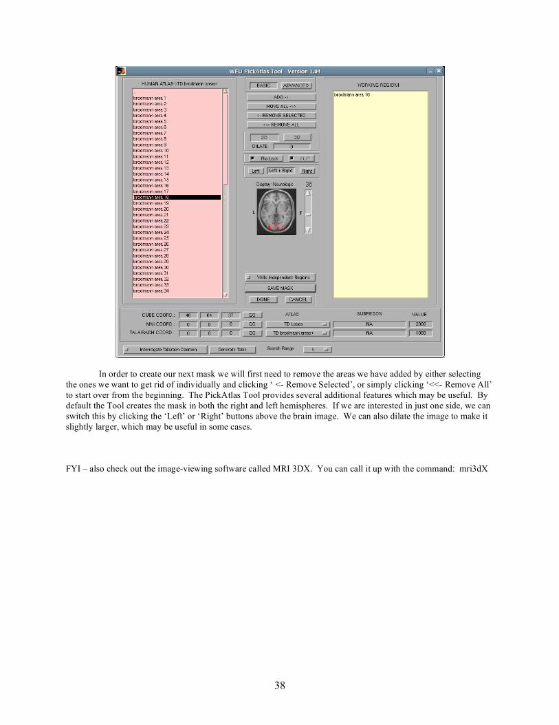
38

In order to create our next mask we will first need to remove the areas we have added by either selecting the ones we want to get rid of individually and clicking ‘ <- Remove Selected’, or simply clicking ‘<<- Remove All’ to start over from the beginning. The PickAtlas Tool provides several additional features which may be useful. By default the Tool creates the mask in both the right and left hemispheres. If we are interested in just one side, we can switch this by clicking the ‘Left’ or ‘Right’ buttons above the brain image. We can also dilate the image to make it slightly larger, which may be useful in some cases. FYI – also check out the image-viewing software called MRI 3DX. You can call it up with the command: mri3dX

39

Chapter 8: Remote Access While it’s usually easiest to do most of our work in the neuroimaging lab, sometimes it’s necessary to be able to work from somewhere else. Luckily for us, there are a variety of methods for remote access. The first methods allow us to log in to a remote system and work on it as if we were working locally. This gives us the advantage of being able to work on much more powerful systems when all we have handy is a low powered system. We can do this both through the command line and graphically. The second method of remote access allows us to access AFS from our local machine, allow us to work on the remote files as if they were local. This is quite handy for the few times we have to use a program that isn’t available on Linux.

Using SSH for Command Line Remote Access We have already experienced the most basic form of remote access when we were converting the data from the scanner. Using the secure shell, ssh, is the simplest way to remotely access another system. Once logged in we can do all of the same command line activities we would do locally in the lab. This allows us to start scripted processes from home or to check up on results without having to run into the lab. Due to the small amount of data that actually has to be sent between the local and remote host, there will appear to be very little slowdown compared to working locally, even on a slow internet connection. As a reminder, the format for the command is as follows, with the only argument being the server to connect to: [meg@dbic-lab_x86-64_04 ~]$ ssh sulcus.cns meg@sulcus.cns's password: Last login: Tue Aug 29 11:18:03 2006 from dbic-lab_x86-64_04.kiewit.dartmouth.edu [meg@sulcus ~] >

In some cases it is necessary to provide a single option before the argument, that of ‘-l username’. This is necessary if you are logged into a system as a different user, alerting the system to what user you will be logging in as. There are a few servers available to us for remote access, such as sulcus.cns, medulla.cns, and putamen.cns. Note that if you are trying to access these servers from outside of the Dartmouth network, you need to fully type out there domain names, such as sulcus.cns.dartmouth.edu. Within the Dartmouth network this is taken care of for you automatically. You can use the secure shell even if you are not using Linux. It is available in Mac OS X if you open up a Terminal window, which can be found in the Utilities program folder. You can then issue a ssh command in the Terminal command line, just as you would in Linux. Be sure to include the ‘-l username’ option if you are doing it this way. In order to do command line based remote access in Windows it is necessary to download a program called PuTTY, which is available for free at the following website: http://www.chiark.greenend.org.uk/~sgtatham/putty/download.html. When run, PuTTY will ask us to enter the server we are trying to connect to, and then will prompt us for our username and password. It will then run exactly the same as ssh on other systems.

Using VNC for Graphical Remote Access Often times it is necessary to work remotely using programs which can only be run using the graphical interface. In order to do this remotely we will be using a method called VNC. VNC is actually a pair of programs, one which runs on the remote server you will be working on, and one that runs locally. In order to begin we need to start the VNC server on the remote machine we will be connecting to. To do this we must first use the method described above to connect using ssh. Once connected we can start the server by issuing the vncserver command.

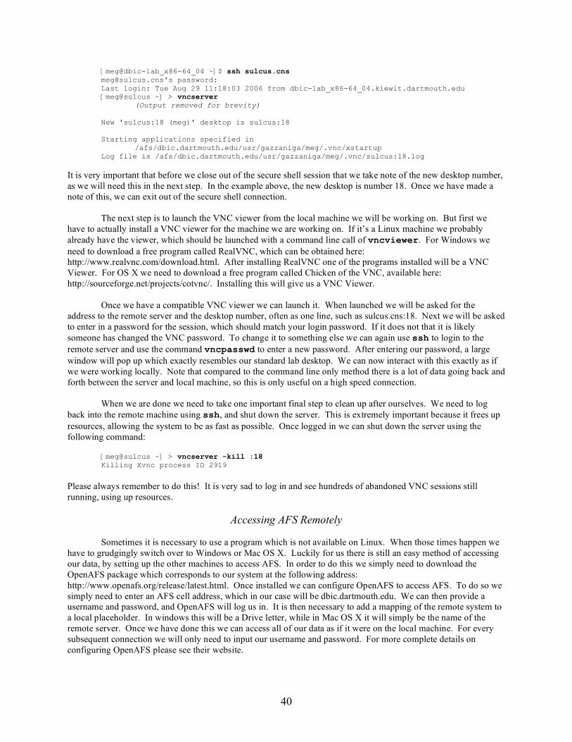
40

[meg@dbic-lab_x86-64_04 ~]$ ssh sulcus.cns meg@sulcus.cns's password: Last login: Tue Aug 29 11:18:03 2006 from dbic-lab_x86-64_04.kiewit.dartmouth.edu [meg@sulcus ~] > vncserver (Output removed for brevity) New 'sulcus:18 (meg)' desktop is sulcus:18

Starting applications specified in /afs/dbic.dartmouth.edu/usr/gazzaniga/meg/.vnc/xstartup

Log file is /afs/dbic.dartmouth.edu/usr/gazzaniga/meg/.vnc/sulcus:18.log It is very important that before we close out of the secure shell session that we take note of the new desktop number, as we will need this in the next step. In the example above, the new desktop is number 18. Once we have made a note of this, we can exit out of the secure shell connection. The next step is to launch the VNC viewer from the local machine we will be working on. But first we have to actually install a VNC viewer for the machine we are working on. If it’s a Linux machine we probably already have the viewer, which should be launched with a command line call of vncviewer. For Windows we need to download a free program called RealVNC, which can be obtained here: http://www.realvnc.com/download.html. After installing RealVNC one of the programs installed will be a VNC Viewer. For OS X we need to download a free program called Chicken of the VNC, available here: http://sourceforge.net/projects/cotvnc/. Installing this will give us a VNC Viewer. Once we have a compatible VNC viewer we can launch it. When launched we will be asked for the address to the remote server and the desktop number, often as one line, such as sulcus.cns:18. Next we will be asked to enter in a password for the session, which should match your login password. If it does not that it is likely someone has changed the VNC password. To change it to something else we can again use ssh to login to the remote server and use the command vncpasswd to enter a new password. After entering our password, a large window will pop up which exactly resembles our standard lab desktop. We can now interact with this exactly as if we were working locally. Note that compared to the command line only method there is a lot of data going back and forth between the server and local machine, so this is only useful on a high speed connection. When we are done we need to take one important final step to clean up after ourselves. We need to log back into the remote machine using ssh, and shut down the server. This is extremely important because it frees up resources, allowing the system to be as fast as possible. Once logged in we can shut down the server using the following command: [meg@sulcus ~] > vncserver -kill :18 Killing Xvnc process ID 2919

Please always remember to do this! It is very sad to log in and see hundreds of abandoned VNC sessions still running, using up resources.

Accessing AFS Remotely

Sometimes it is necessary to use a program which is not available on Linux. When those times happen we have to grudgingly switch over to Windows or Mac OS X. Luckily for us there is still an easy method of accessing our data, by setting up the other machines to access AFS. In order to do this we simply need to download the OpenAFS package which corresponds to our system at the following address: http://www.openafs.org/release/latest.html. Once installed we can configure OpenAFS to access AFS. To do so we simply need to enter an AFS cell address, which in our case will be dbic.dartmouth.edu. We can then provide a username and password, and OpenAFS will log us in. It is then necessary to add a mapping of the remote system to a local placeholder. In windows this will be a Drive letter, while in Mac OS X it will simply be the name of the remote server. Once we have done this we can access all of our data as if it were on the local machine. For every subsequent connection we will only need to input our username and password. For more complete details on configuring OpenAFS please see their website.