Biophys. J. in press

Diffusion of the Reaction Boundary of Rapidly Interacting Macromolecules in Sedimentation Velocity

Peter Schuck

Dynamics of Macromolecular Assembly, LBPS, National Institute of Biomedical Imaging and Bioengineering, National Institutes of Health, Bethesda, MD 20892

Keywords: protein interactions, reaction/diffusion/convection systems, analytical ultracentrifugation, sedimentation velocity, Lamm equation, Gilbert-Jenkins theory

Peter Schuck, Ph.D. DMA/LBPS/NIBIB National Institutes of Health 13 South Drive, Bldg 13, Rm 3N17 Bethesda, MD 20892 schuckp@mail.nih.gov

2  

Abstract

Sedimentation velocity analytical ultracentrifugation (SV) combines relatively high hydrodynamic resolution of macromolecular species with the ability to study macromolecular interactions, which has great potential for studying dynamically assembled multi-protein complexes. Complicated sedimentation boundary shapes appear in multi-component mixtures when the time-scale of the chemical reaction is short relative to the time-scale of sedimentation. Although the Lamm partial differential equation (Lamm PDE) rigorously predicts the evolution of concentration profiles for given reaction schemes and parameter sets, this approach is often not directly applicable to data analysis due to experimental and sample imperfections, and/or due to unknown reaction pathways. Recently, we have introduced the effective particle theory (EPT), which explains quantitatively and in a simple physical picture the sedimentation boundary patterns arising in the sedimentation of rapidly interacting systems (Biophys. J. (2010) Vol. 98 Number 9). However, it does not address the diffusional spread of the reaction boundary from the co-sedimentation of interacting macromolecules, which also has been of long-standing interest in the theory of SV. Here, EPT is exploited to approximate the concentration gradients during the sedimentation process, and to predict the overall, gradient-average diffusion coefficient of the reaction boundary. The analysis of the heterogeneity of the sedimentation and diffusion coefficients across the reaction boundary shows that both are relatively uniform across the parameter space. These results support the application of diffusion-deconvoluting sedimentation coefficient distributions c(s) to the analysis of rapidly interacting systems, and provides a framework for the quantitative interpretation of the diffusional broadening and the apparent molar mass values of the effective sedimenting particle in dynamically associating systems.

3  

Introduction

In the last decade, sedimentation velocity analytical ultracentrifugation (SV) has re-emerged as a powerful technique for the study of interacting macromolecules. It has unique potential for the detection of size, shape, composition, and thermodynamic equilibrium constants of complexes in slow or rapid chemical equilibrium with their free constituent species. In particular, SV is well-suited to address the often most difficult problem of establishing the number and stoichiometry of multiple co-existing complexes, and to determine the reaction scheme. At the same time, the hydrodynamic and spectral resolution provides the virtue of SV being relatively robust against the presence of many kinds of impurities and aggregates. The technique has been reviewed, for example, in (1-5).

The technique has a long history spanning almost a century of theoretical and practical application to protein interactions. Driven by increased interest in the study of protein interactions, the last decade brought many significant advances, especially in the computational modeling of SV. The underlying partial differential equations (PDE) of SV, the Lamm equation, can now be solved sufficiently fast and precise so that it can be used for fitting by non-linear regression of experimental raw data sets on ordinary laboratory computers. This brought the modern techniques of directly and globally fitting the equations for the sedimentation/diffusion/reaction PDE of certain reaction schemes to experimental data (6-9), as well as the determination of diffusion deconvoluted, high-resolution sedimentation coefficient distributions (10), size-and-shape distributions (11), and multi-signal sedimentation coefficient distributions for multi-component systems (12).

Despite this computational progress, many phenomena have remained less well understood on a biophysical level. As has been pointed out by Gilbert & Jenkins already 50 years ago, systems of interconverting species with instantaneous reactions on the time-scale of sedimentation migrate very differently from populations of non-interconverting species (13), in ways perhaps unexpected and non-intuitive when unfamiliar with the migration of interacting systems (14). Of course, any behavior is captured in the solutions to the partial differential equations of sedimentation, but this alone is insufficient to understand the mechanisms of coupled transport. It also does not help us to understand rules for how the system parameters relate to each other when the system is exhibiting a certain phenomenology. However, such knowledge is important to develop robust experimental designs and methodology for the data analysis, and, in particular, to fully exploit the unique potential of SV in the study of multi-component interactions.

To this end, we have recently introduced the effective particle theory (EPT) that explains, in a simple physical picture, the basic rules that govern the formation of sedimentation boundary patterns of multi-component mixtures (i.e., the division of the sedimenting system into a slowly migrating single-component ‘undisturbed boundary’ and a rapidly migrating ‘reaction boundary’ containing a mixture of all species) (15). EPT highlights, for the first time, the existence of a phase transition in parameter space, where the singularity occurs that the entire reacting system

4  

sediments in a single boundary, the latter sedimenting with a velocity unequal any of the species’ velocities. Across this phase transition line, the constituent of the slow boundary switches. EPT also describes how the asymmetry of the individual free species’ velocities translates into an asymmetry of this phase transition line in the parameter space of loading concentrations. EPT provides simple quantitative expressions for the amplitudes and velocities of all boundary components, as well as the phase transition. This facilitates data analysis approaches based on modeling the isotherms of boundary patterns as a function of loading concentration, which constitute robust, information-rich binding isotherms (15,16), and enables the extension of this approach to more complex interaction schemes. The experimental observables of SV across the parameter space of loading concentrations, as predicted by EPT, as well as the molecular mechanism of coupled reaction and sedimentation for given parameters, can be visualized in the effective particle explorer tool of the software SEDPHAT (a biophysical data analysis software for interacting systems (17)).

However, with its basis on mass balance considerations across the reaction boundary, EPT is only concerned with the sedimentation coefficients and amplitudes of the sedimentation boundaries. It does not address the questions of the detailed boundary shape. In particular, the diffusive properties of the reaction boundaries is an area that has so far remained comparatively poorly explored. Yet, it is of high practical interest, since de-convolution of diffusion affords highly increased hydrodynamic resolution. Again, the basic computational recipe provided by the sedimentation/diffusion/reaction PDE equations provides a rigorous predictive tool for the evolution of concentration gradients given a certain parameter set, but it does not satisfactorily explain the relationships between the observables across the parameter space of loading concentrations. In particular, the set of Lamm PDEs of reacting systems does not define the magnitude of the ‘average’ diffusion coefficient of the reaction boundary, as well as the variation across the reaction boundary from this average value.

The ‘constant bath’ approximation, originally developed by Krauss and co-workers (18) and later re-discovered by Urbanke, Witte & Curth (19), predicts that reaction boundaries diffuse with a single, weight-average diffusion coefficient. This is consistent with the observation that c(s) distribution of non-interacting species (10) can model concentration profiles from reacting systems remarkably well (9). Even though qualitatively the results of the constant bath theory are very good, and the accuracy of the predicted sedimentation coefficients is excellent, the predictions for the diffusion coefficient are less successful (9). Further, the constant bath approximation cannot be applied well across the whole parameter space of loading concentrations (9) due to the neglect of co-sedimentation of both free components in the reaction boundary.

The present work explores a different approach to arrive at an approximate analytical expression for the diffusion properties of the reaction boundaries across the entire parameter space. It is physically motivated, and exploits the relationships arising in EPT that are valid for any parameter combination to approximate the concentration gradients in the reaction boundary. We

5  

show this compares well with best-fit diffusion coefficients to reaction boundaries from exact solutions of the sedimentation/diffusion/reaction PDE. Finally, the consequences for diffusional deconvolution with sedimentation coefficient distribution c(s) and size-and-shape distributions are discussed.

Theory

Let us consider a bimolecular reaction of A + B AB in instantaneous equilibrium characterized by the mass action law cAB = KcAcB with association equilibrium constant K (or equilibrium dissociation constant KD = 1/K). Let us choose the nomenclature of A and B such that A is the slower sedimenting species. The initial loading concentrations of A and B are cAtot,0 and cBtot,0, respectively.

Lamm equations

The propagation of the system after start of centrifugation at the angular velocity ω is given by the Lamm PDE, which can be written generally as

<1>

with k denoting the species A, B, and AB, sk and Dk the species’ sedimentation and diffusion coefficients, and ck(r,t) the local radial and time-dependent concentration of the species (14). qk denote the reaction fluxes that have the constraint from mass conservation qA = qB = qAB . The absence of hydrodynamic non-ideality (i.e. a concentration-dependence of sk and Dk is assumed throughout. Eq. <1> can be solved numerically with the software SEDPHAT for given parameter sets, but this does not further illuminate the physical processes of sedimentation.

For rapid self-associating systems, in order to simplify the Lamm PDE and to eliminate the reaction fluxes, it is customary to condense all species’ equations into a single PDE in terms of total local concentration and concentration-dependent, locally weight-average sedimentation coefficient and gradient-average diffusion coefficient, respectively. It is possible to express the Lamm PDE of heterogeneous associations similarly in terms of constituent concentrations cAtot(r,t)=cA(r,t)+cAB(r,t) and cBtot(r,t)=cB(r,t)+cAB(r,t)

<2>

with the local weight-average sedimentation and gradient average diffusion coefficients

2 21k kk k k k

c cc s r D r q

t r r rω

⎡ ⎤∂∂ ∂ ⎢ ⎥+ − =⎢ ⎥∂ ∂ ∂⎣ ⎦

2 2

2 2

1( , ) ( , ) 0

1( , ) ( , ) 0

Atot AtotAtot A B Atot Atot A B

Btot BtotBtot A B Btot Btot A B

c cs c c c r D c c r

t r r r

c cs c c c r D c c r

t r r r

ω

ω

⎡ ⎤∂ ∂∂ ⎢ ⎥+ − =⎢ ⎥∂ ∂ ∂⎣ ⎦⎡ ⎤∂ ∂∂ ⎢ ⎥+ − =⎢ ⎥∂ ∂ ∂⎣ ⎦

6  

<3>

and the symmetrical expressions

1

1( , ) , ( , )

11

A BB AB A B

B A ABBtot A B Btot A B

A A BA B

c cD D K c c

r rs c Kss c c D c c

c K c cK c c

r r

−

−

⎡ ⎤⎛ ⎞∂ ∂⎢ ⎥⎟⎜ ⎟+ + ⎜⎢ ⎥⎟⎜ ⎟⎜⎢ ⎥∂ ∂⎝ ⎠+ ⎣ ⎦= =⎡ ⎤+ ⎛ ⎞∂ ∂⎢ ⎥⎟⎜ ⎟+ + ⎜⎢ ⎥⎟⎜ ⎟⎜⎢ ⎥∂ ∂⎝ ⎠⎣ ⎦

<4>

(A detailed derivation is in the Supporting Material.) A typical set of concentration gradients evolving during the sedimentation of an interacting system is shown in Figure 1A. The boundary pattern exhibits a division into an undisturbed boundary that consists entirely of either free A or free B, and the reaction boundary that exhibits coupled migration of all free and complex species (13,15).

Effective Particle Theory

The propagation of the undisturbed boundary is trivial, except for the question which component provides this undisturbed boundary, and the question of the concentration in the undisturbed boundary. In EPT (15), this component is denoted as ‘secondary component’, abbreviated ‘Y’ and the component that is not ‘secondary’ is termed ‘dominant’ and abbreviated as ‘X’. Y is equal to A for ,0 ,0Btot Btotc c∗< , and Y is equal to B for ,0 ,0Btot Btotc c∗> , with the phase transition

,0,0 ,0 ,0

4 ( )( )( ) 1 1

2 ( ) ( )Atot AB BB A

Btot Atot AtotAB B AB A

c K s ss sc c c

K s s s s∗

⎛ ⎞−− ⎟⎜ ⎟⎜= + + + ⎟⎜ ⎟⎜ ⎟− − ⎟⎜⎝ ⎠ <5>

. The undisturbed boundary vanishes at the phase transition point ,0 ,0Btot Btotc c∗= . The

concentration of the undisturbed boundary is

, ,0

( )1

( ) ( )AB Y

Y undist Ytot ABY AB Y X Y

s sc c c

Kc s s s s

⎛ ⎞− ⎟⎜ ⎟= − +⎜ ⎟⎜ ⎟⎜ − + −⎝ ⎠ <6>

The reaction boundary contains mixtures of free X and complex AB at the initial equilibrium concentration (i.e., co-sedimenting cX,co = cX,0), as well as free Y at the concentration cY,co = cY,0 – cY,nudist . They sediment as ergodic system, where the fractional time-average states of

1

1( , ) , ( , )

11

B AA AB B A

A B ABAtot A B Atot A B

B B AB A

c cD D K c c

r rs c Kss c c D c c

c K c cK c c

r r

−

−

⎡ ⎤⎛ ⎞∂ ∂⎢ ⎥⎟⎜ ⎟+ + ⎜⎢ ⎥⎟⎜ ⎟⎜∂ ∂⎢ ⎥⎝ ⎠+ ⎣ ⎦= =⎡ ⎤+ ⎛ ⎞∂ ∂⎢ ⎥⎟⎜ ⎟+ + ⎜⎢ ⎥⎟⎜ ⎟⎜∂ ∂⎢ ⎥⎝ ⎠⎣ ⎦

7  

molecules X and Y being bound or free are equal to their population fractions, and such that the time-average velocities of molecules X and Y are equal, assuming a value

X X AB ABA B

X AB

c s c ss

c c

+=

+ <7>

This can be illustrated best in a movie (20). EPT is only concerned with the total fluxes arising from the sedimentation of the reaction boundary and the undisturbed boundary, and the concentration profiles are thus approximated as step-functions, as illustrated in Figure 1B. EPT does not make statements regarding the boundary shape or diffusion.

Diffusion coefficients of the reaction boundary

If the components are instantaneously linked by mass action law at all times, it should be possible to approximate the diffusive broadening of the reaction boundary by a single diffusion coefficient of the system, A BD . We expect that both components contribute to diffusion, and

that the magnitude of A BD is weighted by each components fluxes. Thus, we hypothesize that the average diffusion coefficient should take the form of a gradient average

Xtot X Ytot YA B

X Y

D c r D c rD

c r c r

∂ ∂ + ∂ ∂=

∂ ∂ + ∂ ∂ <8>

We note that exact expressions for DAtot and DBtot are available in Eqs. <3> and <4>. Their evaluation requires knowledge of the concentration gradients Ac r∂ ∂ and Bc r∂ ∂ , similar to

Eq. <8>.

We can make use of the knowledge of the concentration differences in EPT to approximate the concentration gradients. As visualized by the dotted lines in Figure 1A, a linear concentration increase across a radial range Δr may serve at least as a first approximation. This leads to

,0X Xc r c r∂ ∂ ≈ Δ , ,0 ,( )Y Y Y undistc r c c r∂ ∂ ≈ − Δ , and XY ABc r c r∂ ∂ ≈ Δ . Inserted in Eqs.

<3>, <4>, and <8>, the boundary width Δr cancels out, and yields

,0 ,0 ,,0 ,0 ,

,0 ,0 ,

,0 ,0 ,

( )( )

( )

( )

X X AB AB Y Y Y undist AB ABX Y Y undist

X AB Y Y undist ABA B

X Y Y undist

D c D c D c c D cc c c

c c c c cD

c c c

+ − ++ −

+ − +≈

+ − <9>

One may further use the Svedberg equation to define an ‘apparent molar mass’ of the effective particles in the reaction boundary of

    <10> (1 )

A BA B

A B

s RTM

D v ρ=

−

8  

Sedimentation coefficient distributions

The sedimentation coefficient distribution c(s) describes the evolution of the experimental signal profiles a(r,t) as a superposition of Lamm equation solutions 1( , , , )s M r tχ of non-interacting species,

1( , ) ( ) ( , ( ), , )a r t c s s M s r t ds≅ χ∫ <11>

(10), where M(s) is usually calculated as a function of s-value following the power-law

( ) 3/20( ) ( ) , ,w

M s k f f sρ η≈ <12>

, and typically fit with the average frictional ratio 0( )w

f f as an adjustable fitting parameter (21),

although other relationships are possible and available in the ultracentrifugal data analysis software SEDFIT (17).

Analogously, the size-and-shape distribution is

1( , ) ( , ) ( , , , )a r t c s M s M r t dsdMχ≅ ∫   <13>

, although it is usually calculated in a more convenient form of c(s,f/f0) (11).

Both Eqs. <11> and <13> are discretized and phrased into a linear least-squares problem for the calculation of the distribution. High-resolution distributions can be calculated conveniently on desktop computers, using established computational tools that yield a mathematically well-defined best-fit solution for this linear least squares fit (22). Since the analysis is ill-posed, it must be combined with regularization techniques to avoid detail not warranted by the data. All data analysis was done with the software SEDFIT, using maximum entropy or Tikhonov regularization. 1

                                                            1 We note that Eq. <13> can generally not be solved accurately with Demeler’s 2DSA method (23), which may be considered a heuristic approach motivated by Eq. <13> , as shown in (22). 

9  

Results

The performance of the approximation Eq. <9> was by calculating exact Lamm equation solutions via Eq. <1> for a variety of conditions, and by extracting estimates for the diffusion coefficients from these boundary profiles. In the absence of hydrodynamic non-ideality, this can be accomplished through fitting the concentration profiles with the c(s) model (see below).

Broadening of the reaction boundary arises not only from diffusion, but also from the heterogeneity of the sedimentation coefficient distribution, as predicted in the asymptotic boundaries by Gilbert-Jenkins theory (13). Even though the range of s-values is very narrow, except for conditions close to the phase transition line (15) (see below), the exquisite sensitivity of SV to the polydispersity of s-values makes this an important contribution. The polydispersity of the s-values in the reaction boundary can be captured by modeling the concentration profiles with a continuous c(s) distribution across the range from approximately sB to sAB.

Polydispersity results in exponentially time-dependent broadening of the boundary. This is independent of the diffusive, i.e. the t -dependent, component of the reaction boundary broadening. The latter can be extracted by adjusting a signal-average frictional ratio of the c(s) distribution to its best-fit value (see below). The undisturbed boundary is modeled as a discrete species with sedimentation parameters of the free component Y predicted from EPT. For conditions where the c(s) peak of the reaction boundary is resolved from the discrete species of the undisturbed boundary, integration of c(s) then provides a value for sA B. Together with sA B , the best-fit frictional ratio implies an estimate of the average molecular weight as well as the average diffusion coefficient (via the Svedberg equation), which may be taken as estimates ofDA B, and MA B, and be compared with the approximations Eqs. <7>, <9>, and <10>, respectively.

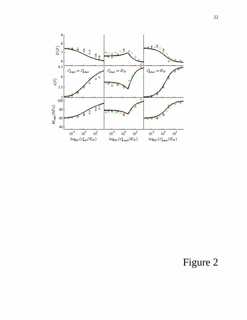
The test-system used was that of a 40 kDa, 3.5 S molecule ‘A’ rapidly interacting with a 60 kDa, 5.0 S molecule ‘B’, to form a 100 kDa, 6.5 S complex. The sedimentation profiles were predicted for a 10 mm solution column at 50,000 rpm, and signals a(r,t) = εAcA(r,t) + εBcB(r,t) + εABcAB(r,t) were calculated in 10 min time-intervals, using signal increments that would be typical with the interference optical detection for these molecules. The parameter space of loading concentrations was explored along different trajectories of equimolar concentrations and titration series of constant A or constant B, respectively. The results of the simulated experiments are shown in Figures 2 and 3, where the circles depict the values derived from the fit of the simulated sedimentation data (PDE solution), and the solid lines depict the isotherms predicted by Eqs. <7>, <9>, and <10>, respectively. It should be noted that there is no adjustable parameter in the solid lines.

One basic prediction from the derivation above is that the values for sA B, DA B, and MA B should be independent of the species’ signal increments. This is at variance with the results from Gilbert-Jenkins theory that the contributions of the free components A and B to the asymptotic

10  

boundaries are not proportional to each other (13). This dilemma motivates a test of the extent of a dependence of the observed diffusion coefficients in the reaction boundary on the species signal contributions.

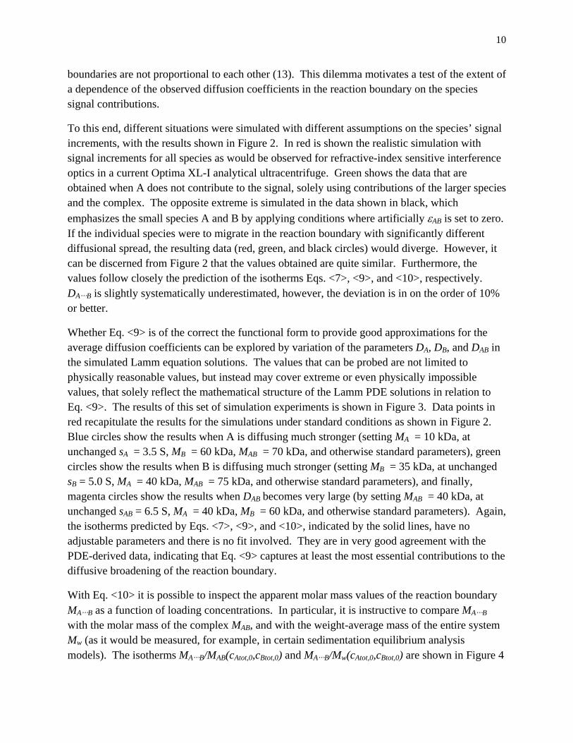
To this end, different situations were simulated with different assumptions on the species’ signal increments, with the results shown in Figure 2. In red is shown the realistic simulation with signal increments for all species as would be observed for refractive-index sensitive interference optics in a current Optima XL-I analytical ultracentrifuge. Green shows the data that are obtained when A does not contribute to the signal, solely using contributions of the larger species and the complex. The opposite extreme is simulated in the data shown in black, which emphasizes the small species A and B by applying conditions where artificially εAB is set to zero. If the individual species were to migrate in the reaction boundary with significantly different diffusional spread, the resulting data (red, green, and black circles) would diverge. However, it can be discerned from Figure 2 that the values obtained are quite similar. Furthermore, the values follow closely the prediction of the isotherms Eqs. <7>, <9>, and <10>, respectively. DA B is slightly systematically underestimated, however, the deviation is in on the order of 10% or better.

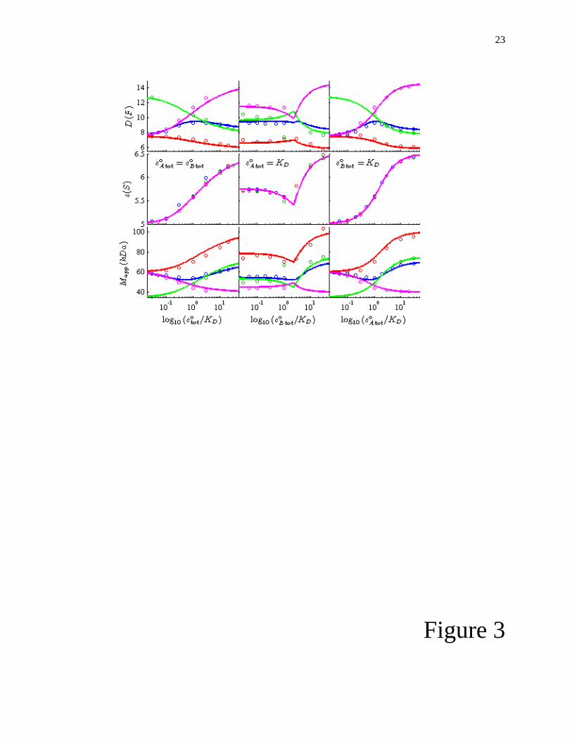
Whether Eq. <9> is of the correct the functional form to provide good approximations for the average diffusion coefficients can be explored by variation of the parameters DA, DB, and DAB in the simulated Lamm equation solutions. The values that can be probed are not limited to physically reasonable values, but instead may cover extreme or even physically impossible values, that solely reflect the mathematical structure of the Lamm PDE solutions in relation to Eq. <9>. The results of this set of simulation experiments is shown in Figure 3. Data points in red recapitulate the results for the simulations under standard conditions as shown in Figure 2. Blue circles show the results when A is diffusing much stronger (setting MA = 10 kDa, at unchanged sA = 3.5 S, MB = 60 kDa, MAB = 70 kDa, and otherwise standard parameters), green circles show the results when B is diffusing much stronger (setting MB = 35 kDa, at unchanged sB = 5.0 S, MA = 40 kDa, MAB = 75 kDa, and otherwise standard parameters), and finally, magenta circles show the results when DAB becomes very large (by setting MAB = 40 kDa, at unchanged sAB = 6.5 S, MA = 40 kDa, MB = 60 kDa, and otherwise standard parameters). Again, the isotherms predicted by Eqs. <7>, <9>, and <10>, indicated by the solid lines, have no adjustable parameters and there is no fit involved. They are in very good agreement with the PDE-derived data, indicating that Eq. <9> captures at least the most essential contributions to the diffusive broadening of the reaction boundary.

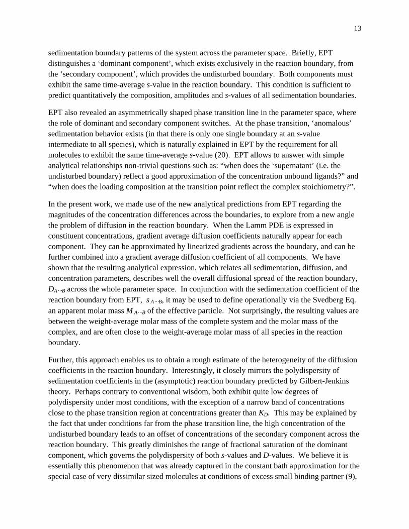
With Eq. <10> it is possible to inspect the apparent molar mass values of the reaction boundary MA B as a function of loading concentrations. In particular, it is instructive to compare MA B with the molar mass of the complex MAB, and with the weight-average mass of the entire system Mw (as it would be measured, for example, in certain sedimentation equilibrium analysis models). The isotherms MA B/MAB(cAtot,0,cBtot,0) and MA B/Mw(cAtot,0,cBtot,0) are shown in Figure 4

11  

Panels A and B, respectively. Not surprisingly, MA B is always between the mass of the complex and the weight-average mass of the entire system. It attains asymptotically the mass of the complex for conditions where the reaction is saturated with excess A and/or excess B, in parallel with the isotherms of sA B approaching the s-value sAB of the complex (as shown in Figure 5 in (15)). On the other hand, MA B is close to the weight-average mass of all species in the loading mixture when the loading concentrations are in the vicinity of the phase transition line, where the undisturbed boundary vanishes. We note that MA B is not equal to the weight-average molar mass of the material in the reaction boundary, even though the relative difference is less than 5% for the particular conditions of Figure 2 (data not shown).

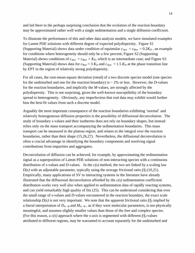
In addition to the average diffusion coefficient DA B across the reaction boundary, we can ask the question how large the local variation of the diffusion coefficient might be, considering that the boundary shape will create regions of different gradients (hence different gradient averages). After all, the boundaries are not linear, as approximated above. Some preliminary estimates are possible based on the observation that the concentration profiles of all species in the reaction boundary take roughly similar shape (for example, in Figure 1A, compare the shapes of the bold red and blue lines in the highlighted region). Even though this is not exactly true, either, it does permit an estimate of the range of diffusion coefficients arising at positions in the boundary. To this end, we may apply the parameterization ,0X Xc kc′ =  and

,0 , ,0 ,( ) ( )Y Y undist Y Y undistc c k c c′− = − with 0,1k ⎡ ⎤∈ ⎣ ⎦ , which explores, in a rough approximation,

the regions of decreasing slopes in the trailing end of the reaction boundary. When inserted into Eq. <9>, a limiting value for 0k = can be found, which provides an estimate for the maximal diffusion coefficient ,maxA BD in the trailing edge of the reaction boundary. In Figure 5A, this

information has been presented in the form of the relative change ( ),maxA B A B A BD D D− as

a function of loading concentration. Even though a considerable spread of diffusion coefficients between the average value DA B and the maximum value DA B,max may be encountered, the region of greater than 10% variation (plotted in cyan and warmer colors) extends very narrowly along the phase transition line. For most of the parameter space, the relative variation with this estimate appears to be less than 5 %.

It is interesting to compare this with the relative variation of s-values in the reaction boundary, as predicted by the asymptotic boundaries in Gilbert-Jenkins theory (13) (denoted as diffusion-free velocity distributions ˆdc dv , customarily using the symbol v to denote the constant sedimentation

velocity in linear geometry). The relative variation of s in the reaction boundary may be assessed by comparing the width and average of the asymptotic velocity distribution predicted by Gilbert & Jenkins, i.e. ( )max min GJv v v− where ˆ ˆ( ) ( )GJv v dc dv dv dc dv dv= ∫ ∫ . This is

shown in Figure 5B across the parameter space for the same system as Figure 2 and Figure 5A. (Similar results are obtained when considering the central second moment instead of the

12  

maximum spread, which is approximately a factor two smaller than the maximum spread; data not shown). For the s-values, similar to the D-values, significant polydispersity is encountered exclusively in a narrow region close to the phase transition line for concentrations cAtot,0 > KD.

Discussion

The diffusional properties of the reaction boundary formed during the sedimentation of rapidly interacting species is a problem of long-standing interest in analytical ultracentrifugation. Even though the Lamm PDE of the interacting system predicts the evolution of the concentration profiles of all species, this alone is not completely satisfactory or sufficient for the optimal planning and evaluation of SV experiments on rapid protein interactions.

Current numerical algorithms and abundant computational resources on desktop computers make routine direct fitting of Lamm PDE solutions of interacting systems to experimental data possible (6-9,24). However, the overwhelming majority of studies in the literature does not apply this approach. This may be attributed to the high susceptibility of the sedimentation boundaries to trace impurities and macromolecular heterogeneity that impede the fit of PDE solutions (9). (An analogous case is the common difficulty of fitting discrete species models to non-interacting mixtures, which is rarely possible, in contrast to the fit of sedimentation coefficient distributions c(s) that can account for trace imperfections, which is very successfully applied in the literature (25).) In addition, the process of establishing the reaction scheme by comparing the performance of various alternate hypothesized Lamm PDE models would be very cumbersome. For this reason, alternative, more flexible and robust approaches must be developed for the data interpretation.

Maybe most importantly, when the Lamm PDEs are used solely as computational recipes, they do not explain the relationship between the physical sedimentation and concentration parameters that generate a certain features in the concentration profiles. Similarly, while they generate near exact concentration profiles for the set of underlying simulation parameters, they do not allow generalizing observables to different parameter sets, and an overview across the parameter space of loading concentrations, for example, would have to be assembled point-by-point. This impedes optimal experimental design and robust data analysis. A comprehensive overview of the observables as a function of Lamm PDE parameters has not yet been reported, and, as a consequence, major general features of the phase behavior of rapidly interacting systems in SV have been overlooked (see below).

With regard to the sedimentation boundary patterns exhibited by rapidly reacting bi-molecular systems, this problem was addressed recently by EPT (15). In EPT, physically based rules provide simple analytical relationships that describe in excellent approximation the

13  

sedimentation boundary patterns of the system across the parameter space. Briefly, EPT distinguishes a ‘dominant component’, which exists exclusively in the reaction boundary, from the ‘secondary component’, which provides the undisturbed boundary. Both components must exhibit the same time-average s-value in the reaction boundary. This condition is sufficient to predict quantitatively the composition, amplitudes and s-values of all sedimentation boundaries.

EPT also revealed an asymmetrically shaped phase transition line in the parameter space, where the role of dominant and secondary component switches. At the phase transition, ‘anomalous’ sedimentation behavior exists (in that there is only one single boundary at an s-value intermediate to all species), which is naturally explained in EPT by the requirement for all molecules to exhibit the same time-average s-value (20). EPT allows to answer with simple analytical relationships non-trivial questions such as: “when does the ‘supernatant’ (i.e. the undisturbed boundary) reflect a good approximation of the concentration unbound ligands?” and “when does the loading composition at the transition point reflect the complex stoichiometry?”.

In the present work, we made use of the new analytical predictions from EPT regarding the magnitudes of the concentration differences across the boundaries, to explore from a new angle the problem of diffusion in the reaction boundary. When the Lamm PDE is expressed in constituent concentrations, gradient average diffusion coefficients naturally appear for each component. They can be approximated by linearized gradients across the boundary, and can be further combined into a gradient average diffusion coefficient of all components. We have shown that the resulting analytical expression, which relates all sedimentation, diffusion, and concentration parameters, describes well the overall diffusional spread of the reaction boundary, DA B across the whole parameter space. In conjunction with the sedimentation coefficient of the reaction boundary from EPT, s A B, it may be used to define operationally via the Svedberg Eq. an apparent molar mass M A B of the effective particle. Not surprisingly, the resulting values are between the weight-average molar mass of the complete system and the molar mass of the complex, and are often close to the weight-average molar mass of all species in the reaction boundary.

Further, this approach enables us to obtain a rough estimate of the heterogeneity of the diffusion coefficients in the reaction boundary. Interestingly, it closely mirrors the polydispersity of sedimentation coefficients in the (asymptotic) reaction boundary predicted by Gilbert-Jenkins theory. Perhaps contrary to conventional wisdom, both exhibit quite low degrees of polydispersity under most conditions, with the exception of a narrow band of concentrations close to the phase transition region at concentrations greater than KD. This may be explained by the fact that under conditions far from the phase transition line, the high concentration of the undisturbed boundary leads to an offset of concentrations of the secondary component across the reaction boundary. This greatly diminishes the range of fractional saturation of the dominant component, which governs the polydispersity of both s-values and D-values. We believe it is essentially this phenomenon that was already captured in the constant bath approximation for the special case of very dissimilar sized molecules at conditions of excess small binding partner (9),

14  

and led there to the perhaps surprising conclusion that the evolution of the reaction boundary may be approximated rather well with a single sedimentation and a single diffusion coefficient.

To illustrate the performance of this and other data analysis models, we have simulated examples for Lamm PDE solutions with different degree of expected polydispersity. Figure S1 (Supporting Material) shows data under condition of equimolar cAtot = cBtot = 0.2KD , an example for conditions where heterogeneity should only be a few percent; Figure S2 (Supporting Material) shows conditions of cAtot = cBtot = KD, which is an intermediate case; and Figure S3 (Supporting Material) shows data for cBtot = 3 KD and cAtot = 1.5 KD at the phase transition line by EPT in the region of relatively strong polydispersity.

For all cases, the root-mean-square deviation (rmsd) of a two discrete species model (one species for the undisturbed and one for the reaction boundary) is ~ 2% or less. However, the D-values for the reaction boundaries, and implicitly the M-values, are strongly affected by the polydispersity. This is not surprising, given the well-known susceptibility of the boundary spread to heterogeneity. Obviously, any imperfection that real data may exhibit would further bias the best-fit values from such a discrete model.

Arguably the most important consequence of the reaction boundaries exhibiting ‘normal’ and relatively homogeneous diffusion properties is the possibility of diffusional deconvolution. The study of boundary s-values and their isotherms does not rely on boundary shapes, but instead relies only on the mass transport accompanying the sedimentation boundaries. This mass transport can be measured in the plateau region, and relates to the integral over the reaction boundaries, rather than their shape (15,26,27). Nevertheless, the diffusional deconvolution is often a crucial advantage in identifying the boundary components and resolving signal contributions from impurities and aggregates.

Deconvolution of diffusion can be achieved, for example, by approximating the sedimentation signal as a superposition of Lamm PDE solutions of non-interacting species with a continuous distribution of s-values and D-values. In the c(s) method, the two are linked by a scaling law D(s) with an adjustable parameter, typically using the average frictional ratio f/f0 (10,21). Empirically, many applications of SV to interacting systems in the literature have already illustrated that the diffusional deconvolution afforded by the c(s) sedimentation coefficient distribution works very well also when applied to sedimentation data of rapidly reacting systems, and can yield remarkably high quality of fits (25). This can be understood considering that over the small range of s-values and D-values encountered in the reaction boundary, the exact scale relationship D(s) is not very important. We note that the apparent frictional ratio f/f0 implied by a literal interpretation of DA B and MA B , as if they were molecular parameters, is not physically meaningful, and assumes slightly smaller values than those of the free and complex species. (For this reason, a c(s) approach where the s-axis is segmented with different f/f0-values attributed to different regions, may be warranted to account separately for the undisturbed and

15  

possibly other clearly visible boundaries; a variety of such models are implemented in SEDFIT and SEDPHAT.) 

In all cases of Figures S1 – S3, the fit with c(s) in the standard form, with an adjustable frictional ratio parameter, is very good although not perfect. With values of ~ 1% or better, the rmsd is approximately a factor two better than a discrete model. Due to the ill-posed nature of the distribution analysis, the sedimentation coefficient distribution does not exactly follow the asymptotic boundary shapes predicted by Gilbert-Jenkins theory (shown as blue area patches), but they were shown to be highly consistent when using Bayesian regularization (28). Close to the phase transition, even the standard maximum entropy regularization can lead to the qualitatively correct bimodal reaction boundary shape. As already shown in Figure 3, the implicit c(M)-values of the reaction boundary peaks (using the conversion of c(s) to c(M) on the basis of a fitted f/f0 parameter of the reaction boundary) follow closely the expected values of Eqs. <9> and <10>.

The size-and-shape distribution, most conveniently expressed as c(s,f/f0), promises an even more detailed analysis accounting for polydispersity in both s and D. However, additional peaks arise at s-values and f/f0- values that are not predicted by the theory (Panels D of Figures S1 – S3). The rmsd is improved by another factor of two relative to the c(s) analysis, but the additional flexibility of the size-and-shape distribution model seems to extract features more detailed than warranted by the quality of the approximations above for rapidly interacting systems. These features are well-defined, but other than the integrals over the undisturbed and reaction boundary features being measures of the respectively mass balance, and the resulting relationship to the overall weight-average s-value sw and the average s-value of the reaction boundary sA B, they currently do not appear to be usefully interpretable.

In conclusion, diffusional deconvolution and analysis of the reaction boundary spread appears to be conducted best with the c(s) method. The present work sheds further light on the relationship of the sedimentation coefficient distributions with the theoretically expected asymptotic boundaries and EPT, and clarifies the meaning of the M-values encountered with the reaction boundaries in the transformation of c(s) to c(M). Since the spread of the sedimentation coefficient distribution is generally small, there will be little influence from using different scaling laws in c(s), as long as they have in some form an adjustable parameter for the magnitude of diffusion.

Conceptually, it should be possible to fit isotherms of Mapp-values extracted from the reaction boundary of experimental data of rapid interacting multi-component systems to the theoretical expressions of MA B(cAtot,cBtot) based on Eqs. <9> and <10> to analyze binding constants. This would give an additional isotherm data set with independent information that could be fit globally with appropriate interaction models, in conjunction with the isotherm of sA B(cAtot,cBtot), sw(cAtot,cBtot), and the boundary amplitudes aundist(cAtot,cBtot) and areact(cAtot,cBtot) introduced previously (16) and implemented in SEDPHAT. However, at this point it seems that the

16  

generally very high precision of s-values and the robustness of measuring the amplitudes of the multi-modal boundaries would provide superior information, and maybe not too much might be gained in terms of further diminishing the uncertainty of the derived estimate of the binding constant.

Another useful aspect of the framework presented here is that it can support important qualitative conclusions about the nature of the reaction. Knowing, for example, that the MA B -value of the reaction boundary is very close to the complex molar mass under conditions of 10-fold excess of cAtot or cBtot over KD (Figure 4) may provide an indicator for the complex stoichiometry. The theoretical approach presented here should be straightforward to generalize to multi-site binding, similar to the constant bath theory and EPT.

Acknowledgement

This research was supported by the Intramural Research Program of the National Institute of Biomedical Imaging and Bioengineering, National Institutes of Health.

17  

References

1. Arisaka, F. 1999. Applications and future perspectives of analytical ultracentrifugation. Tanpakushitsu Kakusan Koso 44:82-91.

2. Cole, J. L., J. W. Lary, P. M. T, and T. M. Laue. 2008. Analytical ultracentrifugation: sedimentation velocity and sedimentation equilibrium. Methods Cell Biol 84:143-79.

3. Howlett, G. J., A. P. Minton, and G. Rivas. 2006. Analytical ultracentrifugation for the study of protein association and assembly. Curr Opin Chem Biol 10(5):430-6.

4. Lebowitz, J., M. S. Lewis, and P. Schuck. 2002. Modern analytical ultracentrifugation in protein science: a tutorial review. Protein Sci 11(9):2067-79.

5. Schuck, P. 2007. Sedimentation velocity in the study of reversible multiprotein complexes. In: Schuck P, editor. Protein Interactions: Biophysical Approaches for the study of complex reversible systems. New York: Springer. p 469-518.

6. Urbanke, C., B. Ziegler, and K. Stieglitz. 1980. Complete evaluation of sedimentation velocity experiments in the analytical ultracentrifuge. Fresenius Z. Anal. Chem. 301:139-140.

7. Schuck, P. 1998. Sedimentation analysis of noninteracting and self-associating solutes using numerical solutions to the Lamm equation. Biophys. J. 75:1503-1512.

8. Stafford, W. F., and P. J. Sherwood. 2004. Analysis of heterologous interacting systems by sedimentation velocicty: curve fitting algorithms for estimation of sedimentation coefficients, equilibrium and kinetic constants. Biophys Chem 108:231-243.

9. Dam, J., C. A. Velikovsky, R. Mariuzza, C. Urbanke, and P. Schuck. 2005. Sedimentation velocity analysis of protein-protein interactions: Lamm equation modeling and sedimentation coefficient distributions c(s). Biophys J 89:619-634.

10. Schuck, P. 2000. Size distribution analysis of macromolecules by sedimentation velocity ultracentrifugation and Lamm equation modeling. Biophys. J. 78:1606-1619.

11. Brown, P. H., and P. Schuck. 2006. Macromolecular Size-And-Shape Distributions by Sedimentation Velocity Analytical Ultracentrifugation. Biophys. J. 90:4651-4661.

12. Balbo, A., K. H. Minor, C. A. Velikovsky, R. Mariuzza, C. B. Peterson, and P. Schuck. 2005. Studying multi-protein complexes by multi-signal sedimentation velocity analytical ultracentrifugation. Proc Natl Acad Sci U S A 102:81-86.

13. Gilbert, G. A., and R. C. Jenkins. 1956. Boundary problems in the sedimentation and electrophoresis of complex systems in rapid reversible equilibrium. Nature 177:853-854.

14. Fujita, H. 1975. Foundations of ultracentrifugal analysis. New York: John Wiley & Sons. 15. Schuck, P. 2010. Sedimentation patterns of rapidly reversible protein interactions. Biophys J 98(9):in

press. 16. Dam, J., and P. Schuck. 2005. Sedimentation velocity analysis of protein-protein interactions:

Sedimentation coefficient distributions c(s) and asymptotic boundary profiles from Gilbert-Jenkins theory. Biophys J 89:651-666.

17. Schuck, P. 2010. https://sedfitsedphat.nibib.nih.gov/software/default.aspx. 18. Krauss, G., A. Pingoud, D. Boehme, D. Riesner, F. Peters, and G. Maass. 1975. Equivalent and non-

equivalent binding sites for tRNA on aminoacyl-tRNA synthetases. Eur. J. Biochem. 55:517-529. 19. Urbanke, C., G. Witte, and U. Curth. 2005. A sedimentation velocity method in the analytical

ultracentrifuge for the study of protein-protein interactions. In: Nienhaus GU, editor. Protein-Ligand Interactions: Methods and Applications. Totowa: Humana Press. p 101-113.

20. Schuck, P. https://sedfitsedphat.nibib.nih.gov/tools/Reaction%20Boundary%20Movies/Forms/AllItems.aspx

21. Schuck, P., M. A. Perugini, N. R. Gonzales, G. J. Howlett, and D. Schubert. 2002. Size-distribution analysis of proteins by analytical ultracentrifugation: strategies and application to model systems. Biophys J 82(2):1096-1111.

22. Schuck, P. 2009. On computational approaches for size-and-shape distributions from sedimentation velocity analytical ultracentrifugation. Eur Biophys J.

18  

23. Brookes, E., W. Cao, and B. Demeler. 2009. A two-dimensional spectrum analysis for sedimentation velocity experiments of mixtures with heterogeneity in molecular weight and shape. Eur Biophys J.

24. Brown, P., and P. Schuck. 2007. A new adaptive grid-size algorithm for the simulation of sedimentation velocity profiles in analytical ultracentrifugation. Comp. Phys. Comm. 178:105-120.

25. Schuck, P. 2010. http://www.analyticalultracentrifugation.com/references.htm. 26. Schachman, H. K. 1959. Ultracentrifugation in Biochemistry. New York: Academic Press. 27. Schuck, P. 2003. On the analysis of protein self-association by sedimentation velocity analytical

ultracentrifugation. Anal. Biochem. 320:104-124. 28. Brown, P., A. Balbo, and P. Schuck. 2007. Using prior knowledge in the determination of

macromolecular size-distributions by analytical ultracentrifugation. Biomacromolecules 8:2011-2024.

29. Gilbert, L. M., and G. A. Gilbert. 1978. Molecular transport of reversibly reacting systems: Asymptotic boundary profiles in sedimentation, electrophoresis, and chromatography. Methods Enzymol 48:195-211.

19  

Figure Legends:

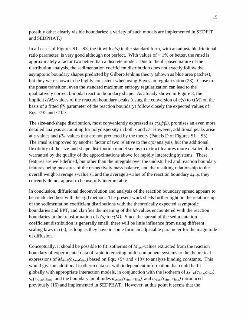
Figure 1: Schematic representation of the concentration gradients in the reaction boundary. Panel A: Concentration profiles of free A (100 kDa, 7 S, red), free B (200 kDa, 10 S, blue) and complex (13 S, black) species during the sedimentation of the interacting system A + B ↔ AB in

the limit of instantaneous reaction, for the conditions at equimolar loading concentrations at KD shown in (9). For clarity, only the concentration profiles from time-points 300 sec and 1,500 sec (thin lines) and 3,000 sec (bold lines) are superimposed. The vertical dashed lines and the range highlighted in red indicate the radial range that covers 10 – 90 % of the reaction boundary at 3,000 sec. The dotted diagonal lines are linear approximations of the gradients in the reaction boundary. Panel B: Schematics of the boundary structure described in EPT, with the division of the secondary component into the undisturbed boundary with concentration cY,undist and the co-sedimenting free fraction cY,co, as well as the concentration of the free species of the dominant component cX and the complex cAB in the reaction boundary. All quantities cY,undist , cY,co, cX , and cAB , as well as the question which component plays the role of dominant and secondary component X and Y are analytically predicted in EPT as a function of loading concentration, equilibrium constant, and all species s-values. We may assign a finite boundary width Δr to the reaction boundary, and approximate it as a constant gradient.

Figure 2: Testing the observed diffusional spread of the reaction boundary for a dependence on the detection of different species. Shown here are diffusion coefficient DA B (top row), sedimentation sA B (middle row), and apparent molar mass MA B (bottom row), observed in the reaction boundary (circles), in comparison with the corresponding predictions Eq. <7>, <9>, and <10>, respectively (solid lines). To determine the data points for the reaction boundary parameters, exact Lamm PDE solutions were calculated for a molecule A of 40 kDa, 3.5 S rapidly interacting with a molecule B of 60 kDa, 5.0 S to form a 100 kDa, 6.5 S complex, sedimenting at 50,000 rpm in a 10 mm solution column, for equimolar dilution series (left column), titration of A with varying B (middle column), and titration of B with varying A (right column). The signal profiles were fitted (excluding the back-diffusion region) with a combination of a Lamm equation solution for a discrete non-interacting species describing the undisturbed boundary and a c(s) distribution describing the reaction boundary. Where the c(s) peak could be well-resolved from the discrete species, it was integrated to determine the average diffusion coefficient DA B , sedimentation coefficient sA B, and apparent molar mass values MA B. Shown in red are simulations using extinction coefficients that would be realistic for interference optical detection (red: εA = 110,000 fringes M-1cm-1, εB = 165,000 fringes M-1cm-

1, and εAB = 275,000 fringes M-1cm-1). In green are shown data obtained from simulations with invisible A, as may be possible in the selective absorbance optical system (green: εA = 0, εB = 165,000 OD M-1cm-1, and εAB = εB). In black is shown an unphysical simulation of a system with invisible complex (black: εA = 110,000 fringes M-1cm-1, εB = 165,000 OD M-1cm-1, and

20  

εAB = 0). The theoretical isotherms are independent of the species’ signal increments, and have no adjustable parameters.

Figure 3: Probing the diffusive properties of the reaction boundary for different systems. The presentation is analogous to Figure 2: the circles indicate the values extracted via c(s) from the Lamm PDE solutions (using standard interference optical signal increments of εA = 110,000 fringes M-1cm-1, εB = 165,000 fringes M-1cm-1, and εAB = 275,000 fringes M-1cm-1), and the solid lines are the isotherms predicted by Eq. <7>, <9>, and <10> for diffusion coefficient DA B (top row), sedimentation sA B (middle row), and apparent molar mass MA B (bottom row), respectively. In red are shown the results for the standard conditions for a molecule A of 40 kDa, 3.5 S rapidly interacting with a molecule B of 60 kDa, 5.0 S to form a 100 kDa, 6.5 S complex. Blue, green, and magenta depict analogous simulations under conditions that are unphysical, but probe extreme values for species’ diffusion coefficients: a 10 kDa molecule A (blue); a 35 kDa molecule B (green), and a 40 kDa complex (magenta).

Figure 4: Isotherms of the apparent molar mass MA B in the parameter space of total loading concentrations, as predicted by Eq. <10>. Shown are the ratios MA B/MAB(cAtot,0,cBtot,0) (Panel A) and MA B/Mw(cAtot,0,cBtot,0) (Panel B), for the system of Figure 2, in a contour plot with the color temperature scale as indicated on the right. The phase transition line of the sedimenting system is indicated as black dashed line.

Figure 5: Polydispersity of the reaction boundary. Panel A: Estimate for the variation of the diffusion coefficient across the reaction boundary, as a function of loading concentration. Shown are values of ( ),maxA B A B A BD D D− using the color temperature scale on the right,

where ,maxA BD is estimated for the trailing edge of the reaction boundary. High values > 0.1

are located in a very narrow band along the phase transition line (shown as dashed line) for concentrations cA > KD. Panel B: Polydispersity of the sedimentation coefficients based on the asymptotic boundaries ˆdc dv from Gilbert-Jenkins theory. Plotted are the relative width

( )max min GJv v v− with ˆ ˆ( ) ( )GJv v dc dv dv dc dv dv= ∫ ∫ , where ˆdc dv was calculated with the

numerical method described by Gilbert & Gilbert (29), using a division of 10,000 concentration values, and maxv and minv are the upper and lower limit of s -values for which > 0.

ˆdc dv

 

F

Figure

21 

e 1

22  

Figure 2

23  

Figure 3

 

F

Figure

24 

e 4

 

Fig

gure 5

25 

5