Embed Size (px)
Citation preview
[09:14 7/12/2017 rdx022.tex] RESTUD: The Review of Economic Studies Page: 511 511–557
Review of Economic Studies (2018) 85, 511–557 doi:10.1093/restud/rdx022© The Author 2017. Published by Oxford University Press on behalf of The Review of Economic Studies Limited.Advance access publication 6 April 2017
Differential Taxation andOccupational Choice
RENATO GOMESToulouse School of Economics, CNRS, University of Toulouse Capitole
JEAN-MARIE LOZACHMEURToulouse School of Economics, CNRS, University of Toulouse Capitole
and
ALESSANDRO PAVANNorthwestern University
First version received August 2014; Editorial decision February 2017; Accepted March 2017 (Eds.)
We develop a framework to study optimal sector-specific taxation, where each agent chooses anoccupation by comparing her skill differential with the tax burden differential across sectors. Becauseskills are not perfectly transferable, the Diamond–Mirrlees theorem (according to which the second-bestentails production efficiency) fails: social welfare can be increased by inducing some agents to join thesector in which their productivity is not the highest. At the optimum, income taxes balance the marginallosses from inter-sector migration with the marginal gains from tailoring tax schedules to the distributionof productivities in each sector (“tagging”). A calibrated model indicates that sector-specific taxationgenerates substantive welfare gains when skill transferability decreases with income, as it enables thegovernment to increase average taxes on high earners with large wage premia.
Key words: Income taxation, Occupational choice, Sales taxes, Sector-specific taxation, Productionefficiency.
JEL Codes: C72, D62
1. INTRODUCTION
The sharp rise in income inequality experienced by advanced economies in the last forty years hasspurred intense research on how skills affect remuneration in different sectors of the economy.Recent empirical contributions document large differences on how various sectors/occupationsaffect inequality measures. For instance, Bell and Van Reenen (2014) show that the financialsector is responsible for most of the increase in the income share held by the top 1% in the U.K.1
A recent study by Bloom et al. (2016) based on a rich data set of administrative records confirmsthat the increase of income inequality in the U.S. in the last three decades is primarily drivenby an increase in the dispersion of compensation across firms and occupations. In contrast, paydifferences within firms have remained virtually unchanged.2
1. For similar evidence for the U.S. and France, see, respectively, Bakija et al. (2012) and Godechot (2012).2. See also Guvenen and Kuruscu (2012).
511
Downloaded from https://academic.oup.com/restud/article-abstract/85/1/511/3108823by Northwestern University School of Law Library useron 24 January 2018
[09:14 7/12/2017 rdx022.tex] RESTUD: The Review of Economic Studies Page: 512 511–557
512 REVIEW OF ECONOMIC STUDIES
The dynamics of compensation across different quantiles of the income distribution alsovary significantly across sectors: in finance, for instance, the increase in compensation hasbeen primarily concentrated at the very top.3 As documented by Kaplan and Rauh (2010) andBakija et al. (2012), occupations in real state and legal services also experienced a significantgrowth in top incomes, whereas top incomes in manufacturing, transportation, and constructiongrew at a more moderate rate.
These empirical observations accord with a renewed interest on taxation policies thatdiscriminate according to the sector where income is generated.4 One notable example is the so-called “bonus tax” in the U.K., according to which the bonuses received by financial employeeswould be taxed at a higher rate than wage income.5 Similar proposals, involving, for instance, adifferent tax treatment of CEO pay or special tax schedules for certain sectors (such as financeor manufacturing) are often debated in the U.S. At the root of these policy proposals is thebelief that certain sectors exceedingly remunerate occupation-specific skills. This may be due totechnological reasons, labour market frictions, or economic rents stemming from imperfectionsin competition and regulation (which are typically out of the scope of the tax authority).6
It is perhaps surprising that, notwithstanding their natural appeal, policies advocating fordifferential taxation across sectors receive little support from the optimal taxation literature.At the heart of the matter lies the celebrated theorem of Diamond and Mirrlees (1971), whichshows that, when the government can levy differentiated (possibly nonlinear) taxes on all factors(input and output), the economy should lie at the production efficient frontier. Strikingly, at theoptimum, distortions in consumption induced by income taxation do not translate into distortionsin production. This result has important implications for the design of tax systems. For instance,it provides an intellectual justification for opposing the taxation of intermediate goods, as well asfor the use of differential sales taxes, or sector-specific income tax regimes. Differential taxationwould create a wedge between productivities and wages across sectors, thus leading to distortionsin the allocation of labour across sectors and undesirable violations of production efficiency.
One key assumption of the Diamond–Mirrlees theorem is that skills are perfectly transferableacross sectors. In this article, we provide a framework for studying optimal differential taxationin settings where the degree of skill transferability is heterogeneous across individuals andoccupations.7 As our results show, this realistic feature has important implications for theoptimality of production efficiency, and the design of income tax schedules.
Our analysis embeds a Mirrleesian taxation problem into an occupational choice model à laRoy (1951), where the agents’ productivities are sector-specific. Agents compare wage levelsand the tax burden across occupations, and then choose which sector to work in, along withtheir labour supply. To isolate the impact of taxation on the production side of the economy, weassume that the goods produced in different sectors are perfect substitutes. The technology in eachsector is described by a representative firm with a linear production function, which rules outgeneral equilibrium effects or externalities across sectors. Accordingly, in our model, the notion
3. See Philippon and Reshef (2012) for evidence for the U.S., and Denk (2015) for eighteen European countries.4. Many countries engage in such policies. Algeria, for example, levies a corporate income tax of 25% on trade
activities and services, and 19% on manufacturing, construction, and tourism. Other countries employing sector-specificincome taxes include Morocco, Tunisia, Luxembourg, and Israel. The use of sector-specific sales taxes is even morecommon; France is a notable example for its very fine sectoral classification (resulting in many tax regimes).
5. The bonus tax was levied in the 2009/10 tax year in the U.K. This tax made employers in the financial sectorpay a 50% tax rate for any (pay-for-performance) bonus paid to employees in excess of 25,000 pounds. Proposed as aone-off event in the aftermath of the financial crisis, this tax collected 2.3 billion pounds.
6. See Philippon and Reshef (2012) for a discussion of this point centered in the U.S. financial sector.7. There is diverse empirical evidence documenting that skill transferability across sectors decreases with income,
and varies from sector to sector. See, for example, Bakija et al. (2012) and Denk (2015), among others.
Downloaded from https://academic.oup.com/restud/article-abstract/85/1/511/3108823by Northwestern University School of Law Library useron 24 January 2018
[09:14 7/12/2017 rdx022.tex] RESTUD: The Review of Economic Studies Page: 513 511–557
GOMES ET AL. DIFFERENTIAL TAXATION AND OCCUPATIONAL CHOICE 513
of production efficiency coincides with that of occupational choice efficiency: agents should jointhe sector in which they are most productive. The government wishes to implement a second bestredistributive tax system à la Mirrlees (1971) using a rich set of sector-specific taxes. We allowthe government’s objective to be Ralwsian or concave utilitarian.
We start with the general case in which the government can use sector-specific nonlinearincome tax schedules. The government can observe the income and the sector chosen by eachindividual, but cannot control the individual’s choice of labour supply or of sector of employment.Accordingly, the government maximizes welfare subject to the usual intensive-margin incentiveconstraints associated with the choice of labour supply by each individual, as well as an extensive-margin incentive constraint associated with the occupational choice by each individual. The multi-dimensionality of each agent’s productivity plays a key role in the extensive margin constraint,as the agent’s occupational choice is determined by how the agent skill differential across sectorscompares to the difference in the tax burden across sectors.
Our first contribution is to develop a methodology for solving multi-dimensional screeningproblems governed by intensive-margin (labour supply) and extensive-margin (sector choice)decisions. Namely, we proceed by first solving a primal problem, where the occupational choicerule (which determines the sector choice as a function of the worker’s productivity profile) is heldfixed, and the tax system is chosen to maximize welfare subject to implementing that occupationalchoice rule (as well as satisfying the intensive-margin incentive constraints). Next, we solve adual problem, where the tax schedule in a given sector is held fixed, and the tax schedule in theother sector (as well as the occupational choice rule) are chosen to maximize welfare.8
The solution to the primal problem delivers a Mirrlees tax formula generalized to a multi-sector economy with endogenous occupational choice and multi-dimensional types.As in Mirrlees(1971), Diamond (1998), and Saez (2001), the tax schedule balances efficiency and redistributiveconsiderations. Efficiency concerns are captured by elasticity (or behavioural) effects, thatmeasure how individuals adjust labour supply in response to higher marginal taxes. Redistributiveconcerns are captured by direct (or mechanical) effects, that measure how an increase in themarginal tax in a given income bracket increases tax collection in all higher income brackets. Ourcharacterization reveals how the government optimally balances intensive-margin distortions inlabour supply across sectors, as a function of the occupational choice rule to be implemented.
In turn, the solution to the dual problem delivers an Euler equation that determines the optimalallocation of workers across sectors. At the optimum, the marginal loss in tax revenue due to themigration of workers across sectors equalizes the marginal gains from tailoring tax schedules to thedistribution of productivities in each sector (“tagging”). Importantly, when skills are imperfectlytransferable across sectors and income taxes are sector-specific, the Diamond–Mirrlees theoremfails: social welfare is increased by assigning some agents to a sector different from the onein which they are most productive. A similar conclusion holds in the (perhaps more realistic)scenario where the government is not able to tax labour income using a sector-specific schedule,but can levy different sales taxes across sectors. Our analysis then implies the failure of theAtkinson–Stiglitz theorem (according to which, when preferences over consumption and leisureare separable, as they are in our economy, the second-best can be implemented with zero salestaxes). Therefore, the use of differential taxation across sectors is strictly needed to implementthe welfare-maximizing outcome.
The key to these results lies in how the tax system affects the informational costs ofredistribution. Differential taxes allow the government to relax the incentive constraints of high-ability agents whose skills are poorly transferable, at the cost of allocating some low-ability
8. In Section 6, we discuss how this methodology can be applied to other settings, such as nonlinear pricing by amulti-product monopolist and managerial compensation with multiple career options.
Downloaded from https://academic.oup.com/restud/article-abstract/85/1/511/3108823by Northwestern University School of Law Library useron 24 January 2018
[09:14 7/12/2017 rdx022.tex] RESTUD: The Review of Economic Studies Page: 514 511–557
514 REVIEW OF ECONOMIC STUDIES
agents to a sector different from the one in which they are most productive. In particular, atthe production efficient outcome, by appropriately increasing taxes in some sector, the plannercan obtain a first-order reduction in the informational costs of redistribution by incurring onlysecond-order losses in total output.
The trade-off between reducing the informational rents of high earners and inducing skillmisallocation among low earners is key to assessing which sector should be favoured at theoptimum. Our analysis identifies two independent (but related) conditions guaranteeing that onesector (let us say, sector a) should be favoured at the optimum. To describe these conditions,let us identify the degree of skill transferability of a worker with the loss of wage per hour ashe moves away from his most productive sector. Similarly, we say that sector a is more skillintensive than sector b if the former sector has relatively more high earners than the latter, underthe assumption that workers choose the sector where they are most productive (i.e. productionefficiency prevails).
Let sector a be the sector in which the degree of skill transferability is the lowest among low-productivity workers and the highest among high-productivity ones, and assume both sectorsare equally skill intensive. At the optimum, taxes in sector a should be lower than in sector b,inducing workers to migrate from the latter sector to the former. Intuitively, tilting the tax systemin favour of sector a (by making the tax burden in sector b heavier than in sector a) entails (1) alower opportunity cost from the migration of low-productivity agents away from the sector inwhich they are most productive, and (2) higher gains in tax collection from high-ability agentsremaining in the sector in which they are most productive. This is the skill transferability motivefor differential taxation.
Alternatively, let both sectors have the same degree of skill transferability at all productivitylevels, but assume that sector b is more skill intensive than sector a. Once again, at the optimum,taxes should be higher in sector b than in sector a, inducing certain workers to migrate from theformer sector to the latter. Intuitively, favouring sector a rather than b entails (1) a lower massof low-productivity agents migrating to the sector in which they are least productive, and (2) ahigher volume of high-productivity agents paying larger taxes in the sector in which they aremost productive. This is the skill intensity motive for differential taxation.
We quantitatively assess the effects discussed above by calibrating our model using data onwages and industry classification from the U.S. Current Population Survey (CPS). To generateconservative estimates on the gains from differential taxation, we construct two large sectors:manufacturing and services. The manufacturing sector aggregates traditional industries, whilethe services sector contains finance, banking, legal and business services, as well as technology-intensive activities characterized by large returns to occupation-specific skills. We interpret thewage data as generated by a (sub-optimal) uniform tax system where production efficiencyprevails, and construct different scenarios regarding the degree of skill transferability in themanufacturing and services sectors.
Our analysis delivers three main lessons: First, the welfare gains from differential taxationcan be large (of the order of 1.5% of GDP). Moreover, most of these gains are due to the skilltransferability motive: accordingly, the services sector (displaying the lowest degree of skilltransferability at the top) faces the largest tax burden. With a more complex tax system and a finersectorial classification (involving more than two sectors), the importance of the skill intensitymotive for differential taxation is expected to be higher.
Secondly, sales taxes (or, equivalently, payroll taxes) are able to generate roughly half of thewelfare gains from sector-specific income tax schedules. This result suggests that the welfaregains from “simple” tax systems, while non-negligible, are far from the levels delivered by fullyoptimal sector-specific income taxation.
Downloaded from https://academic.oup.com/restud/article-abstract/85/1/511/3108823by Northwestern University School of Law Library useron 24 January 2018
[09:14 7/12/2017 rdx022.tex] RESTUD: The Review of Economic Studies Page: 515 511–557
GOMES ET AL. DIFFERENTIAL TAXATION AND OCCUPATIONAL CHOICE 515
Thirdly, we document the incidence of production inefficiencies and the shape of optimalmarginal tax schedules. We show that differential taxation can increase significantly the averagetax rate faced by high earners in occupations with large wage premia.
The rest of the article is organized as follows. Below, we close the Introduction by brieflyreviewing the most pertinent literature. Section 2 previews the main themes of our analysisthrough a simple discrete-type example. Section 3 presents the continuum-type version of ourmodel. Section 4 characterizes the optimal tax system under differential taxation, and discussesimplications for production efficiency. Section 5 quantifies these results by means of a calibrationexercise. Section 6 discusses a few extensions and concludes.
1.1. Related literature
Our article contributes to the literature on optimal taxation in the tradition of Mirrlees (1971). Ouranalysis is directly related to fundamental results in this literature. First, Diamond and Mirrlees(1971) show that the second-best optimum exhibits production efficiency in a general equilibriumsetting where the government can use (linear) taxes on all inputs and outputs, and firms can betaxed in a lump sum fashion.9 In turn, Atkinson and Stiglitz (1976) show that differentiated salestaxes across goods are detrimental to welfare, when the government can use a nonlinear incometax schedule and preferences are weakly separable between consumption and leisure.10 Theseresults were first challenged by Naito (1999), who considers a two-sector model in which twogoods are produced using skilled and unskilled labour in different intensities. Naito shows that atax/subsidy on one good, implicitly creating a subsidy to low-skilled labour, is always desirableprovided the government can use a nonlinear income tax. This indirect form of wage subsidy (asopposed to a subsidy on total labour income) allows the government to ease redistribution withoutaffecting incentive constraints. This result comes from the fact that the high-skilled individualscannot effectively claim the low-skilled wage. Later, Saez (2004) discusses this assumption andargues that, in the long run, individuals choose their occupation (say, skilled or unskilled). As aconsequence, the optimality of production efficiency and of uniform sales taxes is restored.
In turn, Saez (2002) derives the optimal tax system in a setting where labour supply responsesinvolve an intensive margin (high- or low-paying occupations) as well as an extensive margin(participation in the labour force). One important assumption in Saez (2002, 2004) is that allworkers are equally productive in all occupations, but differ in their tastes for each occupation(including tastes for not working). By contrast, in the spirit of Roy (1951), we assume thatworkers have heterogenous skills across occupations (extensive margin), and make intensive-margin choices within occupation (i.e. hours of work).
Rothschild and Scheuer (2013) consider a two-sector Roy model with endogenous wages (asworkers are paid their marginal product of labour in a constant-returns technology) and assume thattaxation is uniform across sectors (as the income tax schedule is the same across sectors and salestaxes are not considered). In turn, Rothschild and Scheuer (2016) consider an economy whereagents can work in a traditional sector (where private and social returns coincide) or in a rent-seeking sector (which imposes a negative externality on the traditional sector). The theme of thesepapers is how general equilibrium effects (determining relative wages), or externalities acrosssectors, shape the optimal tax system in a world with cross-sector migration and imperfect tagging(uniform taxation).Ales et al. (2015) consider an economy with a continuum of sectors, but whereagents are endowed with a one-dimensional productivity type. They restrict attention to uniform
9. See Hammond (2000) for a generalization of this result that allows for asymmetric information about workers’skills and nonlinear taxation.
10. See Boadway (2012) for a unified treatment of these results.
Downloaded from https://academic.oup.com/restud/article-abstract/85/1/511/3108823by Northwestern University School of Law Library useron 24 January 2018
[09:14 7/12/2017 rdx022.tex] RESTUD: The Review of Economic Studies Page: 516 511–557
516 REVIEW OF ECONOMIC STUDIES
taxation and simulate their model to assess the impact of technical change (which affects relativewages across sectors) on the optimal income tax schedule. In contrast to these contributions, ourmodel allows for sector-specific taxation (in the form of income or sales taxes), but abstractsfrom general equilibrium effects (as technology is linear in our model) and externalities acrosssectors.
Another related contribution is Scheuer (2014), who considers an economy where agents haveone-dimensional skills and choose between being workers or entrepreneurs (with the latter choiceinvolving a setup cost that enters additively in the agents’ utility function). This simple structureof heterogeneity implies that production efficiency is optimal when the government can tax theincomes from wages and profits differently. This feature eliminates the tension between “tagging”gains and inefficiency losses that is at the core of our work.11
Our article is also related to the literature on “tagging”, initiated by Akerlof (1978) and furtherdeveloped by Cremer et al. (2010) and Mankiw and Weinzierl (2010), in the context of optimalnonlinear income taxation. The idea of “tagging” is that the government can increase efficiencyand redistribute more by conditioning income taxes on observable characteristics, such as age,sex, or height. A fundamental difference with respect to our article is that, in this literature, thetagging variable is exogenous (agents cannot respond by changing sex, age, or height). In contrast,in our economy, workers are able to migrate across sectors in response to differential taxation(i.e. the tagging variable is endogenous).
Allowing for endogenous occupational choice naturally leads to a multi-dimensional screeningproblem. Solving such problems is often challenging, as one cannot determine from theoutset the direction in which incentive constraints bind (see Rochet and Choné (1998), and thereferences therein). In our setting, the multi-dimensionality of workers’ productivity only affectssector-choice (extensive-margin) decisions. This allows us to employ the primal–dual approachdescribed above, bringing considerable tractability to the analysis.
As our analysis reveals, the multi-dimensionality of workers’ types has important impli-cations for the design of optimal tax systems. Other recent studies share a similar view:Choné and Laroque (2010) study the optimality of negative marginal taxes in a model whereworkers have a bi-dimensional type comprising a skill level and an outside option that isresponsible for participation in the labour force. Golosov et al. (2013) study optimal nonlinearincome and capital taxes in a model where individuals differ both in their skills and in theirtime preferences. Jacquet and Lehmann (2016) study optimal income taxation when agents areheterogeneous in their skills and behavioural elasticities.
2. PREAMBLE: AN ILLUSTRATIVE EXAMPLE
In order to introduce the main ideas in the simplest possible way, this section studies differentialtaxation in a stylized discrete-type example. Consider a unit-mass continuum of agents and twosectors indexed by j∈{a,b}. We identify the type of each agent with the pair (na,nb) describingthe agent’s productivity in each of the two sectors. The utility of an agent with type (na,nb)working hj hours in sector j and paying t dollars in taxes is hjnj −t−ψ (hj
), where ψ(h) is the
disutility of labour (which, in this example, we assume to be quadratic, i.e. ψ (h)=h2/2).
11. See also Scheuer and Werning (2016) for the analysis of optimal taxation in economies with extensive andintensive margins as well as for a discussion of how the Mirrlees (1971) problem can be recast as a special case ofDiamond and Mirrlees (1971). In this article, as well as in all other papers cited above, taxation is uniform across sectors.
Downloaded from https://academic.oup.com/restud/article-abstract/85/1/511/3108823by Northwestern University School of Law Library useron 24 January 2018
[09:14 7/12/2017 rdx022.tex] RESTUD: The Review of Economic Studies Page: 517 511–557
GOMES ET AL. DIFFERENTIAL TAXATION AND OCCUPATIONAL CHOICE 517
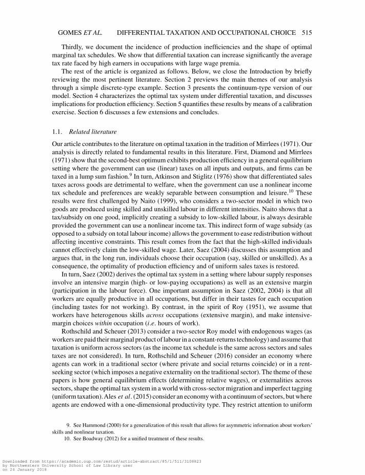
The agents’ types are independently drawn from a distribution with probability mass functionf satisfying
f (n,n−εa)=pa, f (n−εb,n)=pb, f (n,n−δa)=qa, f (n−δb,n)=qb,
where 0<n−εj ≤ n<n−δj ≤ n for j∈{a,b}. Figure 1 depicts the support of f . That is, an agentwith sector-j productivity equal to n (alternatively, n) loses εj (alternatively, δj) dollars per hour ifhe works in sector k �= j. We refer to −εj (alternatively, −δj) as the degree of skill transferabilityamong low-productivity (alternatively, high-productivity) agents in sector j. For convenience, weassume that the two sectors have equal sizes in case all agents work in the sector in which theirproductivity is the highest, that is, pj +qj = 1
2 for j=a,b. We refer to qj/pj as the skill intensity ofsector j, that is, the ratio between high- and low-productivity agents in sector j that obtains whenall agents choose the sector in which their productivity is the highest.
The social planner designs a budget-balanced income tax system to maximize the utility ofthe worst-off agent in the economy (i.e. the planner’s objective function is Ralwsian). Agentscompare productivity levels and the tax burden across sectors and then choose (1) which sectorto work in and (2) the number of hours to supply in the chosen sector.
Foreshadowing the analysis in the next sections, we shall proceed in two steps. In the firststep, we fix which types work in each sector (i.e. the occupational choice rule) and computethe tax system that maximizes social welfare among all tax systems that induce agents to sortthemselves over the two sectors according to the given occupational choice rule. In the secondstep, we compare welfare across occupational choice rules.
Let us consider first the occupational choice rule according to which types (n,n−εa) and(n,n−δa) work in sector a and types (n−εb,n) and (n−δb,n) work in sector b. This rule respectsproduction efficiency, as the labour supply of each agent is employed in the sector in which theagent is most productive.
Under the optimal tax system satisfying production efficiency, the “high” types (n,n−δa) and(n−δb,n) supply labour at the first-best level. The government’s ability to tax these individualsis constrained by their ability to mimic the “low” types (n,n−εa) and (n−εb,n). In the typicalcase where the only binding incentive constraints are the ones regarding the provision of laboursupply within each sector, a sector-j high type obtains the informational rent
uj(n)=uj(n)+ψ (hj(n))−ψ(n
nhj(n)
), (1)
where the schedules uj(·) and hj(·) describe the indirect utility and the labour supply of individualsworking in sector j=a,b. This rent originates in the ability of the most productive agents togenerate the same income as the least productive ones by working less, thus economizing onthe disutility of labour. As a result, the rent for these most productive agents equals the utilityof the least productive agents working in the same sector, augmented by a term that equals thedifferential in the disutility of labour from generating the same income as the least productiveagents. In order to reduce these rents and foster redistribution from the most productive agentsto the least productive ones, the government taxes the labour income of the least productiveagents so as to induce them to work less. At the optimum, the government thus distorts the laboursupplied by the least productive agents downwards relative to the first-best level. We denote by�e the social welfare achieved by the optimal tax system under production efficiency.
Let us now consider the occupational choice rule according to which types (n,n−εa),(n−εb,n) and (n,n−δa) work in sector a, and type (n−δb,n) works in sector b. A tax systemimplementing such a rule is said to favour sector a (see Figure 1 for an illustration).12
12. Analogously, we say that a tax system favours sector b when the only type to work in sector a is (n,n−δa).
Downloaded from https://academic.oup.com/restud/article-abstract/85/1/511/3108823by Northwestern University School of Law Library useron 24 January 2018
[09:14 7/12/2017 rdx022.tex] RESTUD: The Review of Economic Studies Page: 518 511–557
518 REVIEW OF ECONOMIC STUDIES
Figure 1
Agent’s productivities and production efficiency.
Notes: The shaded points describe the support of agent’s productivity pairs. Under production efficiency, types above the 45-degree linework in sector b, while those below it work in sector a. When the tax system favours sector a, all types below the dotted curve work insector a.
Relative to the production efficiency benchmark, this occupational choice rule moves type(n−εb,n) from sectors b to a. While this assignment entails an opportunity cost of εb per hour ofwork (which corresponds to the productivity loss from having this type working in the “wrong”sector), it allows the government to increase tax collection from high-productivity agents workingin sector b (whose type is (n−δb,n)).
To understand why, note that, at the Ralwsian optimum, type (n−δb,n) has to be indifferentbetween (1) working on sector b with productivity n, and (2) migrating to sector a and workingwith productivity n−δb. In case he decides to migrate, the best that this type can do is to mimicagents with productivity n. The optimal tax system leaves type (n−δb,n) perfectly indifferentbetween these two options:
ub(n)=ua(n)+ψ (ha(n))−ψ( n
n−δbha(n)
). (2)
As the comparison with equation (1) reveals, the ability to mimic agents whose productivity isn is hindered by the fact that skill is not perfectly transferable across sectors (i.e. δb>0). As aresult, the government is able to levy higher taxes from type (n−δb,n) than under productionefficiency (and the more so the higher is δb).
Of course, this reduction in the informational costs of redistribution comes at the cost ofmisallocating the hours of work provided by type (n−εb,n). Moreover, this misallocation cost isdecreasing in −εb, which is the degree of skill transferability among low-productivity agents insector b. Denoting by�j the social welfare achieved by the optimal tax system that favours sectorj and recalling that �e is social welfare under the optimal tax system consistent with productionefficiency, we then have the following result:
Result 1. (Production Inefficiency). Production efficiency fails at the optimum whenever thedegree of skill transferability among low-productivity agents in some sector is sufficiently small.Formally, for any j,k ∈{a,b}, k �= j, any δk>0, there exists ε such that �j>�e if and only ifεk<ε.
Downloaded from https://academic.oup.com/restud/article-abstract/85/1/511/3108823by Northwestern University School of Law Library useron 24 January 2018
[09:14 7/12/2017 rdx022.tex] RESTUD: The Review of Economic Studies Page: 519 511–557
GOMES ET AL. DIFFERENTIAL TAXATION AND OCCUPATIONAL CHOICE 519
The proof for both this result and the next one are in the Supplementary Material. Intuitively,the optimal tax system exhibits production inefficiency whenever favouring some sector (andtherefore reducing the informational costs of redistribution) entails low costs in terms of skillmisallocation. As our analysis in the next sections reveals, the analog of this condition in thecontinuum-type case has little bite, and production inefficiency is a robust (or “generic”) featureof the second-best.
In case production inefficiency prevails, which sector should be favoured? The trade-offdiscussed above is key to answering this question. To see why, let both sectors be equally skillintensive, but assume that sector a simultaneously exhibits the lowest degree of skill transferabilityamong low-productivity agents (i.e. εa>εb) and the highest among high-productivity agents(i.e. δa<δb). In this case, welfare is greater by inducing low-productivity agents in sector bto migrate to sector a, relative to the opposite migration pattern. The reason is that favouringsector a, rather than b, entails (1) lower opportunity costs of skill misallocation for each low-productivity agent that migrates, and (2) higher gains in tax collection from each high-abilityagent that stays in the unfavoured sector. This is the skill transferability motive for differentialtaxation.
Another possibility is that both sectors enjoy the same degree of skill transferability for allproductivity levels, but a sector, let us say a, is less skill intensive than the other ( qa
pa<
qbpb
). Inthis case, taxes should be lower in sector a than in sector b. The reason is that favouring sectora, as opposed to favouring b, entails (1) a lower mass of low-productivity agents migratingto their least-productive sector, and (2) a higher mass of high-productivity agents payinglarge taxes in their most productive sector. This is the skill intensity motive for differentialtaxation.
This discussion is summarized in the next result.
Result 2. (Sectorial Bias). Social welfare is higher by favouring sector j rather than sector k �= j,that is, �j>�k, whenever one of the following mutually exclusive conditions hold:
1. Sector j enjoys the lowest degree of skill transferability among low-productivity agentsand the highest among high-productivity agents (i.e. εj>εk and δj<δk), and both sectorsare equally skill intensive (i.e.
qjpj
= qkpk
).
2. Sector j is less skill intensive than sector k (i.e.qjpj<
qkpk
), and both sectors enjoy the same
degree of skill transferability among low and high productivity agents (i.e. εj =εk andδj =δk).
Of course, the case for favouring sector j is only strengthened if the skill transferability motive(εj>εk and δj<δk) and the skill intensity motive (
qjpj<
qkpk
) are present simultaneously. By contrast,
it is a priori unclear which sector should be favoured if the degree of skill transferability isuniformly greater in some sector (e.g. εa>εb and δa>δb), or if the skill transferability motiveand the skill intensity motive point in different directions (e.g. εj>εk and δj<δk , but
qjpj>
qkpk
).
In these cases, the welfare level attained from favouring either sector depends on the magnitudesof the “informational cost” and “skill misallocation” effects discussed above, and a quantitativeanalysis is needed to assess the sectorial bias at the optimum. This often occurs in the continuum-type case, where the bivariate distribution of skills is unlikely to satisfy stringent order relationsacross all productivity levels. We shall come back to this important issue in Section 5, wherewe simulate our model using U.S. income data. Before doing so, we first extend the model to acontinuum of types.
Downloaded from https://academic.oup.com/restud/article-abstract/85/1/511/3108823by Northwestern University School of Law Library useron 24 January 2018
[09:14 7/12/2017 rdx022.tex] RESTUD: The Review of Economic Studies Page: 520 511–557
520 REVIEW OF ECONOMIC STUDIES
3. MODEL AND PRELIMINARIES
3.1. Set-up
We consider an economy with a unit-mass continuum of agents and two sectors indexed byj∈{a,b}.13 The goods produced in the two sectors are assumed to be perfect substitutes, and theirprices are normalized to one. Each agent chooses which sector to work in and the number ofhours (or effort) to supply in the chosen sector. The productivity of an agent in sector j∈{a,b}is denoted by nj ∈N ≡ (n,n), where n>0, n∈R++∪{+∞} and n>n. An agent’s type is thusgiven by the vector n≡ (na,nb) describing the agent’s productivity in each of the two sectors.Each agent’s type is an independent draw from a distribution F with support N≡N2. We assumethat F is absolutely continuous with respect to the Lebesgue measure and denoted by Fj is itsmarginal distribution with respect to the j-dimension (with bounded density fj). The conditionaldistributions are denoted by Fj|k , for j,k ∈{a,b}, j �=k (with bounded density fj|k).
An agent with productivity nj supplying hj ∈R+ hours in sector j∈{a,b} produces njhj unitsof effective labour. The income generated by this agent is then yj =wjnjhj, where wj ∈R+ is thewage per unit of effective labour.
The government taxes labour income according to the (possibly) nonlinear sector-specific taxschedule Tj(yj). For simplicity, we assume that each agent’s utility is quasilinear in consumptionso that the utility of an agent of type n supplying hj hours in sector j is given by
wjhjnj −Tj(wjhjnj)−ψ(hj), (3)
whereψ(h) is the disutility of labour, which we assume takes the isoelastic formψ(h)=h1ξ , with
ξ ∈ (0,1). The elasticity of labour supply with respect to wages is then equal to ξ/(1−ξ ), whichis increasing in ξ .
The production side in each sector is described by a representative neoclassical firm withlinear technology:
Xj =Fj(Lj)=Lj,
where Xj is the amount of good-j produced and where Lj is the amount of effective labour hiredby the firm. Firm j’s profits are then equal to
πj = (1−wj −τj)Lj, (4)
where τj is the sales tax rate on good j.14 The wage rates w≡ (wa,wb), the agents’labour supply, andthe labour demand from the representative firms are all simultaneously determined in equilibrium,as explained below.
3.2. Taxation equilibrium
The occupational choice of each agent is described by the occupational choice rule C :N→{a,b}.This rule specifies for each type n= (na,nb)∈N the sector in which the agent works. In turn, thelabour supply schedules hj :Nj →R+ determine the amount of labour supplied by the agentsworking in sector j as a function of their sector-j productivity, with the domain Nj of each
13. In the Supplementary Material we extend the analysis model to an arbitrary (finite) number of sectors.14. In an alternative interpretation, τj is a payroll tax levied on employers on sector j. For consistency, we shall
favour the sales tax interpretation.
Downloaded from https://academic.oup.com/restud/article-abstract/85/1/511/3108823by Northwestern University School of Law Library useron 24 January 2018

[09:14 7/12/2017 rdx022.tex] RESTUD: The Review of Economic Studies Page: 521 511–557
GOMES ET AL. DIFFERENTIAL TAXATION AND OCCUPATIONAL CHOICE 521
function hj denoting the set of productivity levels of those agents working in sector j.15 For futurereference, for any set Nj ⊂N, we denote by Nj the closure of the set, with N =[n,n].
Hereafter we will refer to an allocation as a triple (C,ha,hb). Next, we define a tax systemT ≡{Ta,Tb,τa,τb} as a collection of sector-specific income tax schedules Tj :R+ →R along withsector-specific sales taxes (or, alternatively, subsidies) τj ∈R. An allocation (C,ha,hb) is said tobe implementable at the wage rates w if there exists a tax system T such that the following fourconditions jointly hold.
The first condition is a consistency property requiring that the domain Nj of each labour supplyfunction hj coincides with the set of productivity levels of those agents working in sector j, asdetermined by the occupational choice rule C. That is,
Na ={na ∈N :∃nb ∈N such that C(na,nb)=a}and symmetrically for sector b.
The second condition is the usual incentive compatibility condition on the intensive marginof labour supply. To describe this condition, let
uj(nj)≡maxh
{wjhnj −Tj(wjhnj)−ψ(h)
}for all nj ∈N, (5)
anduj(nj)≡wjhj(nj)nj −Tj(wjhj(nj)nj)−ψ(hj(nj)) for all nj ∈Nj. (6)
This condition then requires that uj(nj)= uj(nj) for all nj ∈Nj. In order to relate labour supplyschedules and marginal taxes, it is convenient to consider the first-order condition associated withequation (5), which has to be satisfied at any interior point where the schedule Tj is differentiable:
wjnj[1−T ′j (wjhj(nj)nj)]=ψ ′(hj(nj)) (7)
The third condition is an incentive compatibility condition on the extensive margin ofoccupational choice. It requires that each agent working in sector j would not be strictly betteroff by working in sector k �= j:
C(n)= j ⇒ uj(nj)≥ uk(nk) for all n∈N.
Finally, the fourth and final condition requires that by employing the effective labour
Lj =∫{n:C(n)=j}
hj(nj)njdF(na,nb),
each firm j=a,b maximizes profits (4). We incorporate the above four conditions into thedefinition of a taxation equilibrium.
Definition 1. (Taxation Equilibrium). A taxation equilibrium E ≡ (C,ha,hb,T ,w) consists ofan allocation (C,ha,hb), a tax system T , and a pair of wage rates w such that the followingconditions jointly hold:
1. The allocation (C,ha,hb) is implementable at the wage rates w by the tax system T ;
15. Because, if an agent works in sector j, his productivity in sector k �= j does not affect his utility function, theschedules hj do not depend on nk for k �= j.
Downloaded from https://academic.oup.com/restud/article-abstract/85/1/511/3108823by Northwestern University School of Law Library useron 24 January 2018

[09:14 7/12/2017 rdx022.tex] RESTUD: The Review of Economic Studies Page: 522 511–557
522 REVIEW OF ECONOMIC STUDIES
2. The tax system T satisfies the government budget constraint, that is,
∑j∈{a,b}
∫{n:C(n)=j}
(Tj(wjhj(nj)nj)+τjhj(nj)nj
)dF(na,nb)≥B, (8)
where B is the exogenous government budget requirement.
It is convenient to define the indirect utility of an agent with type n under the taxationequilibrium E ≡ (C,ha,hb,T ,w) as
U(n;E)≡uC(n)(nC(n))= maxj∈{a,b}
{uj(nj)
},
where the schedules uj and uj are given by equations (5) and (6), respectively.The government chooses a taxation equilibrium E ≡ (C,ha,hb,T ,w) to maximize a given
welfare function. We focus on two common specifications. The first is a Ralwsian objective,which consists in the utility of the worst-off individual:
�R [U(·;E)]≡minn∈N
{U(n;E)}.
The second welfare function is a generalized utilitarian one, which consists in a concavetransformation of the agents’ utilities:
�CU [U(·;E)]≡∫
n∈Nφ(U(n;E))dF(n),
whereφ is a strictly increasing and weakly concave function reflecting the government preferencesfor redistribution.
We will use the index x=R (alternatively, x=CU) to refer to the Ralwsian (alternatively,concave utilitarian) welfare objective. We will say that a taxation equilibrium is x-optimal if itsolves the respective x-problem and refer to the tax system associated with an x-optimal taxationequilibrium as an x-optimal tax system. For future reference, we define the indicator function1CU
x , which equals zero if x=R, and one if x=CU.
3.3. Implementability
The next lemma characterizes the set of implementable allocations for given wage rates.
Lemma 1. (Implementability). The allocation (C,ha,hb) is implemented at the wage rates w bythe tax system T only if the following conditions jointly hold:
1. For every j∈{a,b}, wages are given by wj =1−τj .2. For every j∈{a,b}, the income schedule yj(nj)≡wjhj(nj)nj is non-decreasing over
Nj. Moreover, the indirect utility schedule uj(nj) is Lipschitz continuous over Nj withderivative equal to
u′j(nj)=ψ ′(hj(nj)
) hj(nj)
njfor almost every nj ∈Nj. (9)
Downloaded from https://academic.oup.com/restud/article-abstract/85/1/511/3108823by Northwestern University School of Law Library useron 24 January 2018
[09:14 7/12/2017 rdx022.tex] RESTUD: The Review of Economic Studies Page: 523 511–557
GOMES ET AL. DIFFERENTIAL TAXATION AND OCCUPATIONAL CHOICE 523
3. The occupational choice rule C can be described by an absolutely continuous andweakly increasing threshold function c :N → N such that C(na,nb)=a if nb<c(na) andC(na,nb)=b if nb>c(na).16 Furthermore, the threshold function c is such that c(na)=nif C(na,nb)=b for all nb ∈N, c(na)=n if C(na,nb)=a for all nb ∈N, and otherwise solvesua(na)=ub(c(na)).
Conversely, suppose the allocation (C,ha,hb), along with the wage rates w and the tax system T ,satisfy the properties in parts 1–3 above, then there exists a tax system T ′ such that the allocation(C,ha,hb) is implemented at the wage rates w by the tax system T ′.
Part 1 shows that, because the technology is linear, labour markets clear if, and only if, themarginal product of labour in each sector, net of sales taxes, equals its marginal cost to the firm.Accordingly, sales taxes affect equilibrium wages in a one-to-one fashion. Part 2 is the standardcharacterization of incentive compatibility on the intensive margin. The envelope condition (9)relates the agents’ indirect utilities to their utility-maximizing labour supply in each sector.
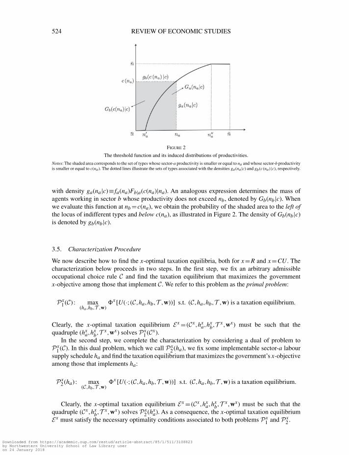
Part 3, in turn, offers a convenient characterization of the extensive margin of occupationalchoice. It establishes that any occupational choice rule can be described by a continuous andnon-decreasing threshold function c that maps na into the sector-b productivity threshold c(na)such that an agent with type n= (na,c(na))∈N is indifferent between working in one sector or theother. We refer to the graph of c as the locus of indifferent types. Because the payoff from workingin a given sector strictly increases with the agent’s productivity in that sector, the threshold c(na)is strictly increasing at any interior point (i.e. at any point where c(na)∈N). This function isinstrumental in describing the distribution of productivities in each sector of the economy.
3.4. Distribution of productivities
Akey feature of the model is that the distribution of productivities within each sector is endogenous(as agents choose in which sector to work in response to the tax system). It is convenient todescribe these distributions in terms of the threshold function c associated with the occupationalchoice rule C. In order to do so, we choose sector labels in the following way. We call sectora the sector for which there is a productivity threshold n′′
a ∈N such c(na)= n for all na ≥n′′a . In
words, all agents whose sector-a productivity is above n′′a work in sector a, irrespective of their
sector-b productivity. If no sector satisfies this property, the choice of labels is arbitrary.17 It isalso convenient to define the threshold n′
a ∈ N such that c(na)>n if and only if na>n′a.18 We will
then say that the occupational choice rule C is admissible if its associated threshold function cis absolutely continuous and strictly increasing over a set (n′
a,n′′a), equal to n for all na<n′
a andequal to n for all na>n′′
a .For such an admissible rule, what is the mass of agents working in sector a whose productivity
does not exceed na? As illustrated in Figure 2, this mass corresponds to the probability of theshaded area below the locus of indifferent types and to the left of na. This is given by
Ga(na|c)≡∫ na
n
∫ c(na)
nf (na,nb)dnbdna =
∫ na
nfa(na)Fb|a(c(na)|na)dna,
16. Recall that N denotes the closure of the set N , that is, N =[n,n].17. For example, consider the threshold function c(n)=n. In this case, no sector satisfies the property described
above, and the choice of labels is arbitrary.18. We let n′
a =n if {na ∈N :c(na)=n}=∅.
Downloaded from https://academic.oup.com/restud/article-abstract/85/1/511/3108823by Northwestern University School of Law Library useron 24 January 2018
[09:14 7/12/2017 rdx022.tex] RESTUD: The Review of Economic Studies Page: 524 511–557
524 REVIEW OF ECONOMIC STUDIES
Figure 2
The threshold function and its induced distributions of productivities.
Notes: The shaded area corresponds to the set of types whose sector-a productivity is smaller or equal to na and whose sector-b productivityis smaller or equal to c(na). The dotted lines illustrate the sets of types associated with the densities ga(na|c) and gb(c(na)|c), respectively.
with density ga(na|c)≡ fa(na)Fb|a(c(na)|na). An analogous expression determines the mass ofagents working in sector b whose productivity does not exceed nb, denoted by Gb(nb|c). Whenwe evaluate this function at nb =c(na), we obtain the probability of the shaded area to the left ofthe locus of indifferent types and below c(na), as illustrated in Figure 2. The density of Gb(nb|c)is denoted by gb(nb|c).
3.5. Characterization Procedure
We now describe how to find the x-optimal taxation equilibria, both for x=R and x=CU. Thecharacterization below proceeds in two steps. In the first step, we fix an arbitrary admissibleoccupational choice rule C and find the taxation equilibrium that maximizes the governmentx-objective among those that implement C. We refer to this problem as the primal problem:
Px1 (C) : max
(ha,hb,T ,w)�x [U(·;(C,ha,hb,T ,w))] s.t. (C,ha,hb,T ,w) is a taxation equilibrium.
Clearly, the x-optimal taxation equilibrium Ex = (Cx,hxa,h
xb,T
x,wx) must be such that thequadruple (hx
a,hxb,T
x,wx) solves Px1 (Cx).
In the second step, we complete the characterization by considering a dual of problem toPx
1 (C). In this dual problem, which we call Px2 (ha), we fix some implementable sector-a labour
supply schedule ha and find the taxation equilibrium that maximizes the government’s x-objectiveamong those that implements ha:
Px2 (ha) : max
(C,hb,T ,w)�x [U(·;(C,ha,hb,T ,w))] s.t. (C,ha,hb,T ,w) is a taxation equilibrium.
Clearly, the x-optimal taxation equilibrium Ex = (Cx,hxa,h
xb,T
x,wx) must be such that thequadruple (Cx,hx
b,Tx,wx) solves Px
2 (hxa). As a consequence, the x-optimal taxation equilibrium
Ex must satisfy the necessary optimality conditions associated to both problems Px1 and Px
2 .
Downloaded from https://academic.oup.com/restud/article-abstract/85/1/511/3108823by Northwestern University School of Law Library useron 24 January 2018

[09:14 7/12/2017 rdx022.tex] RESTUD: The Review of Economic Studies Page: 525 511–557
GOMES ET AL. DIFFERENTIAL TAXATION AND OCCUPATIONAL CHOICE 525
3.6. Production efficiency
We conclude this section by defining production efficiency. The definition below adapts the usualdefinition to the environment studied in this article.
Definition 2. (Production Efficiency). The equilibrium E = (C,ha,hb,T ,w) exhibits productionefficiency if and only if, holding fixed the labour supply of each agent (as specified by theequilibrium E), there exists no reallocation of agents across sectors that yields a higher aggregateoutput. This is the case if and only if the threshold function c associated with the equilibriumoccupational choice rule C is such that c(na)=na for all na ∈N.
This definition is thus the standard one;19 simply notice that, in this economy, fixing the supplyof inputs and changing their usage across firms/sectors is equivalent to holding fixed the laboursupply (i.e. hours of work) of each individual and changing his occupation.
4. OPTIMAL DIFFERENTIAL TAXATION
We study first optimal differential taxation when the government is able to employ sector-specificincome tax schedules. It should come as no surprise that the ability to tailor income taxes tooccupational choice renders sales taxes redundant.
Remark 1. (Effective Tax Schedules). Let E = (C,ha,hb,T ,w) be a taxation equilibrium.There exists another taxation equilibrium E = (C,ha,hb,T ,w) implementing the same allocation(C,ha,hb) and producing the same payoffs under E such that, for j=a,b,
1. the income tax schedules satisfy Tj (y)=τjy+Tj((
1−τj)y),
2. sales taxes and wages are given by τj =0 and wj =1.
Hereafter, we refer to (Ta,Tb) as the “effective tax schedule” of the tax system T .
Intuitively, if the government has enough flexibility in designing sector-specific income taxschedules, it can then always replicate the effects of sales taxes with appropriately chosen incometaxes. As a consequence, it is without loss of optimality to consider taxation equilibria whereτa =τb =0. To lighten notation, we thus drop the wage pair w from the description of taxationequilibria, and write the latter as E = (C,ha,hb,T ), with the implicit understanding that w= (1,1).
Below, we will thus characterize x-optimal taxation equilibria in terms of their effectivetax schedules (and drop the qualification “effective” to lighten the exposition). For simplicity,and following the literature, we will abstract from bunching and corner solutions; that is, we willrestrict attention to economies in which the optimality conditions described below identify incomeschedules yj(nj) that are non-decreasing and such that yj(nj)>0 for all nj ∈Nj (equivalently,hj(nj)>0 for all nj ∈Nj).
4.1. Optimal marginal tax rates
Ley λ denote the multiplier associated with the government budget constraint (8) and denote bymj(nj)≡φ′(uj(nj)
)/λ the ratio of social marginal utility of all individuals with productivity nj
working in sector j to the marginal value of public funds for the government. The next proposition
19. For a textbook treatment, see chapter 5 of Mas-Colell et al. (1995).
Downloaded from https://academic.oup.com/restud/article-abstract/85/1/511/3108823by Northwestern University School of Law Library useron 24 January 2018
[09:14 7/12/2017 rdx022.tex] RESTUD: The Review of Economic Studies Page: 526 511–557
526 REVIEW OF ECONOMIC STUDIES
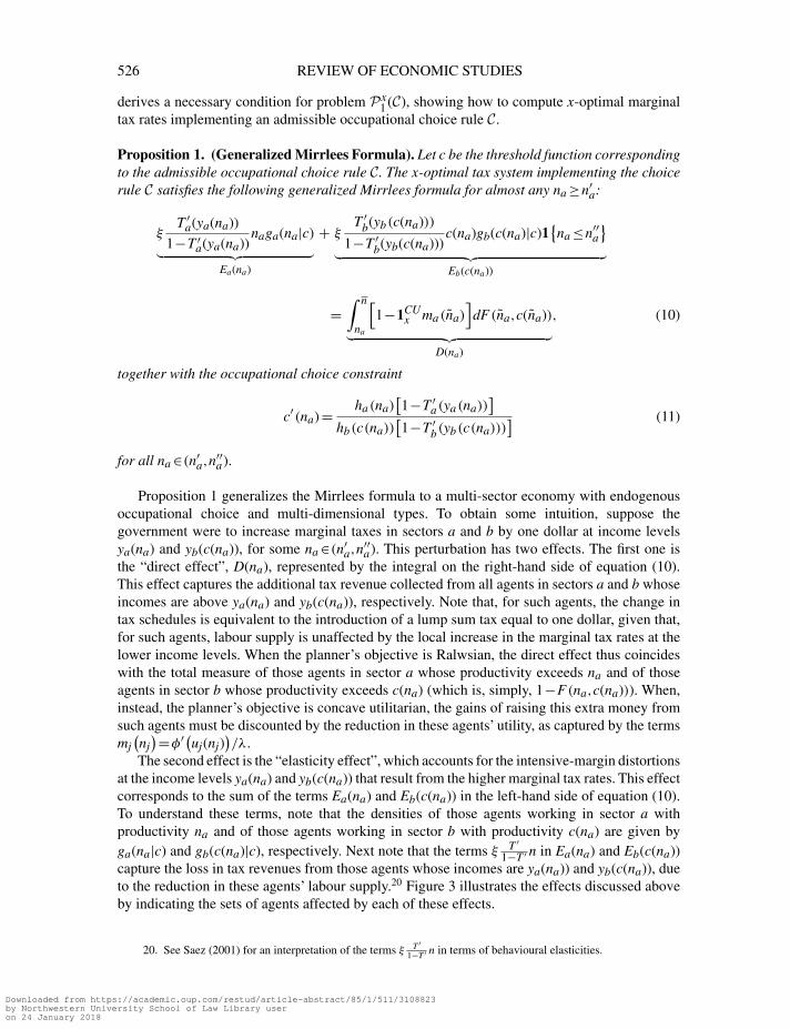
derives a necessary condition for problem Px1 (C), showing how to compute x-optimal marginal
tax rates implementing an admissible occupational choice rule C.
Proposition 1. (Generalized Mirrlees Formula). Let c be the threshold function correspondingto the admissible occupational choice rule C. The x-optimal tax system implementing the choicerule C satisfies the following generalized Mirrlees formula for almost any na ≥n′
a:
ξT ′
a(ya(na))
1−T ′a(ya(na))
naga(na|c)︸ ︷︷ ︸Ea(na)
+ ξT ′
b(yb(c(na)))
1−T ′b(yb(c(na)))
c(na)gb(c(na)|c)1{na ≤n′′
a}
︸ ︷︷ ︸Eb(c(na))
=∫ n
na
[1−1CU
x ma(na)]
dF (na,c(na))︸ ︷︷ ︸D(na)
, (10)
together with the occupational choice constraint
c′(na)= ha(na)[1−T ′
a(ya(na))]
hb(c(na))[1−T ′
b(yb(c(na)))] (11)
for all na ∈ (n′a,n
′′a).
Proposition 1 generalizes the Mirrlees formula to a multi-sector economy with endogenousoccupational choice and multi-dimensional types. To obtain some intuition, suppose thegovernment were to increase marginal taxes in sectors a and b by one dollar at income levelsya(na) and yb(c(na)), for some na ∈ (n′
a,n′′a). This perturbation has two effects. The first one is
the “direct effect”, D(na), represented by the integral on the right-hand side of equation (10).This effect captures the additional tax revenue collected from all agents in sectors a and b whoseincomes are above ya(na) and yb(c(na)), respectively. Note that, for such agents, the change intax schedules is equivalent to the introduction of a lump sum tax equal to one dollar, given that,for such agents, labour supply is unaffected by the local increase in the marginal tax rates at thelower income levels. When the planner’s objective is Ralwsian, the direct effect thus coincideswith the total measure of those agents in sector a whose productivity exceeds na and of thoseagents in sector b whose productivity exceeds c(na) (which is, simply, 1−F (na,c(na))). When,instead, the planner’s objective is concave utilitarian, the gains of raising this extra money fromsuch agents must be discounted by the reduction in these agents’ utility, as captured by the termsmj(nj)=φ′(uj(nj)
)/λ.
The second effect is the “elasticity effect”, which accounts for the intensive-margin distortionsat the income levels ya(na) and yb(c(na)) that result from the higher marginal tax rates. This effectcorresponds to the sum of the terms Ea(na) and Eb(c(na)) in the left-hand side of equation (10).To understand these terms, note that the densities of those agents working in sector a withproductivity na and of those agents working in sector b with productivity c(na) are given byga(na|c) and gb(c(na)|c), respectively. Next note that the terms ξ T ′
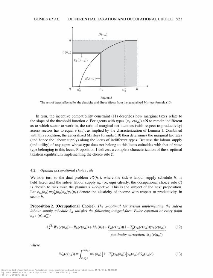
1−T ′ n in Ea(na) and Eb(c(na))capture the loss in tax revenues from those agents whose incomes are ya(na)) and yb(c(na)), dueto the reduction in these agents’ labour supply.20 Figure 3 illustrates the effects discussed aboveby indicating the sets of agents affected by each of these effects.
20. See Saez (2001) for an interpretation of the terms ξ T ′1−T ′ n in terms of behavioural elasticities.
Downloaded from https://academic.oup.com/restud/article-abstract/85/1/511/3108823by Northwestern University School of Law Library useron 24 January 2018
[09:14 7/12/2017 rdx022.tex] RESTUD: The Review of Economic Studies Page: 527 511–557
GOMES ET AL. DIFFERENTIAL TAXATION AND OCCUPATIONAL CHOICE 527
Figure 3
The sets of types affected by the elasticity and direct effects from the generalized Mirrlees formula (10).
In turn, the incentive compatibility constraint (11) describes how marginal taxes relate tothe slope of the threshold function c. For agents with types (na,c(na))∈N to remain indifferentas to which sector to work in, the ratio of marginal net incomes (with respect to productivity)across sectors has to equal c′(na), as implied by the characterization of Lemma 1. Combinedwith this condition, the generalized Mirrlees formula (10) then determines the marginal tax rates(and hence the labour supply) along the locus of indifferent types. Because the labour supply(and utility) of any agent whose type does not belong to this locus coincides with that of sometype belonging to this locus, Proposition 1 delivers a complete characterization of the x-optimaltaxation equilibrium implementing the choice rule C.
4.2. Optimal occupational choice rule
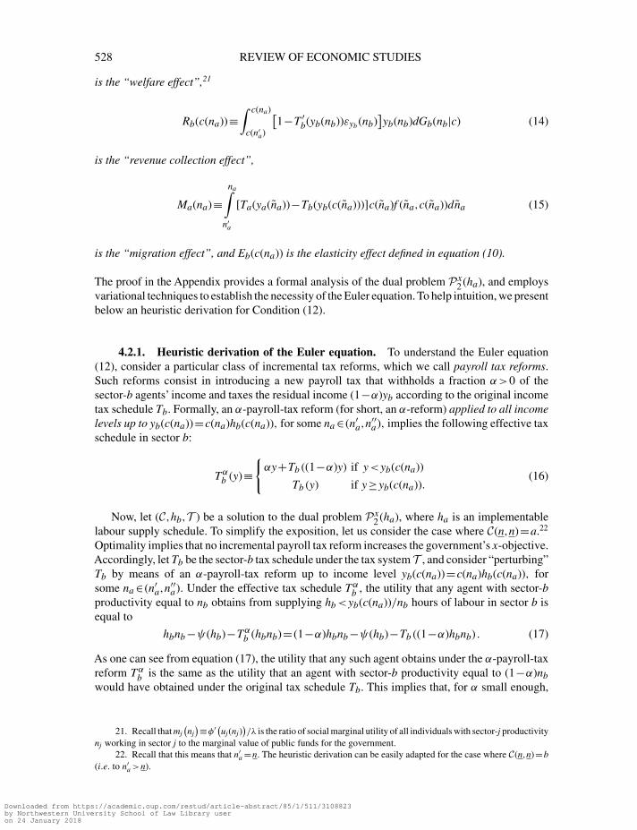
We now turn to the dual problem Px2 (ha), where the side-a labour supply schedule ha is
held fixed, and the side-b labour supply hb (or, equivalently, the occupational choice rule C)is chosen to maximize the planner’s x-objective. This is the subject of the next proposition.Let εyb (nb)≡y′
b(nb)nb/yb(nb) denote the elasticity of income with respect to productivity, insector b.
Proposition 2. (Occupational Choice). The x-optimal tax system implementing the side-alabour supply schedule ha satisfies the following integral-form Euler equation at every pointna ∈ (n′
a,n′′a):
1CUx Wb(c(na))=Rb(c(na))+Ma(na)+Eb(c(na))(1−T ′
b(yb(c(na)))yb(c(na))︸ ︷︷ ︸continuity correction: �b(c(na))
(12)
where
Wb(c(na))≡∫ c(na)
c(n′a)
mb(nb)[1−T ′
b(yb(nb))]yb(nb)dGb(nb|c) (13)
Downloaded from https://academic.oup.com/restud/article-abstract/85/1/511/3108823by Northwestern University School of Law Library useron 24 January 2018
[09:14 7/12/2017 rdx022.tex] RESTUD: The Review of Economic Studies Page: 528 511–557
528 REVIEW OF ECONOMIC STUDIES
is the “welfare effect”,21
Rb(c(na))≡∫ c(na)
c(n′a)
[1−T ′
b(yb(nb))εyb (nb)]yb(nb)dGb(nb|c) (14)
is the “revenue collection effect”,
Ma(na)≡na∫
n′a
[Ta(ya(na))−Tb(yb(c(na)))]c(na)f (na,c(na))dna (15)
is the “migration effect”, and Eb(c(na)) is the elasticity effect defined in equation (10).
The proof in the Appendix provides a formal analysis of the dual problem Px2 (ha), and employs
variational techniques to establish the necessity of the Euler equation. To help intuition, we presentbelow an heuristic derivation for Condition (12).
4.2.1. Heuristic derivation of the Euler equation. To understand the Euler equation(12), consider a particular class of incremental tax reforms, which we call payroll tax reforms.Such reforms consist in introducing a new payroll tax that withholds a fraction α>0 of thesector-b agents’ income and taxes the residual income (1−α)yb according to the original incometax schedule Tb. Formally, an α-payroll-tax reform (for short, an α-reform) applied to all incomelevels up to yb(c(na))=c(na)hb(c(na)), for some na ∈ (n′
a,n′′a), implies the following effective tax
schedule in sector b:
Tαb (y)≡{αy+Tb((1−α)y) if y<yb(c(na))
Tb(y) if y≥yb(c(na)).(16)
Now, let (C,hb,T ) be a solution to the dual problem Px2 (ha), where ha is an implementable
labour supply schedule. To simplify the exposition, let us consider the case where C(n,n)=a.22
Optimality implies that no incremental payroll tax reform increases the government’s x-objective.Accordingly, let Tb be the sector-b tax schedule under the tax system T , and consider “perturbing”Tb by means of an α-payroll-tax reform up to income level yb(c(na))=c(na)hb(c(na)), forsome na ∈ (n′
a,n′′a). Under the effective tax schedule Tαb , the utility that any agent with sector-b
productivity equal to nb obtains from supplying hb<yb(c(na))/nb hours of labour in sector b isequal to
hbnb −ψ(hb)−Tαb (hbnb)= (1−α)hbnb −ψ(hb)−Tb((1−α)hbnb). (17)
As one can see from equation (17), the utility that any such agent obtains under the α-payroll-taxreform Tαb is the same as the utility that an agent with sector-b productivity equal to (1−α)nbwould have obtained under the original tax schedule Tb. This implies that, for α small enough,
21. Recall that mj(nj)≡φ′(uj(nj)
)/λ is the ratio of social marginal utility of all individuals with sector-j productivity
nj working in sector j to the marginal value of public funds for the government.22. Recall that this means that n′
a =n. The heuristic derivation can be easily adapted for the case where C(n,n)=b(i.e. to n′
a>n).
Downloaded from https://academic.oup.com/restud/article-abstract/85/1/511/3108823by Northwestern University School of Law Library useron 24 January 2018
[09:14 7/12/2017 rdx022.tex] RESTUD: The Review of Economic Studies Page: 529 511–557
GOMES ET AL. DIFFERENTIAL TAXATION AND OCCUPATIONAL CHOICE 529
under the α-payroll tax reform Tαb , the indirect utility uαb of each agent with sector-b productivityequal to nb is given by:23
uαb (nb)≡{
ub((1−α)nb) if nb ∈(
c(n′a)
1−α ,c(na))
ub(nb) if nb>c(na).(18)
where ub is the indirect utility function under the original tax schedule Tb. As a consequence,the occupational choice rule under the perturbed schedule Tαb , which we denote by Cα , can bedescribed by a threshold function cα that is a linear transformation
cα(na)= 1
1−α c(na) (19)
of the threshold rule c under the original schedule Tb, for any na<na.Remarkably, as we show below, the Euler equation (12) accounts for the gains and losses of
α-payroll-tax reforms up to income level yb(c(na)). Hereafter, we discuss each of these effects.
• Welfare effect. The first effect is the impact of the reform on the agents’ utility. Fromequation (18), it is easy to see that, at α=0, the marginal effect of an α-reform up toincome level yb(c(na)) on the indirect utility of any agent whose sector-b productivity isnb<c(na) is equal to −nbu′
b(nb). When the government’s objective is concave utilitarian,the importance assigned to this effect, adjusted for the shadow cost of raising money, isgiven by
−m(nb)u′b(nb)nb =−m(nb)
[1−T ′
b(yb(nb))]yb(nb),
where the equality follows from the incentive-compatibility constraint (9) along with thefact that at any point of differentiability of the tax schedule Tb, the optimal choice oflabour supply must satisfy the first-order condition (7). Integrating the expression abovefor all nb<c(na) leads to the welfare effect Wb(c(na)) in the Euler equation, as defined inequation (13). In the case of a Ralwsian objective, this effect is zero, given that the effect oftax reforms on the indirect utility of all agents but the worst-off individuals is disregardedby the planner.
• Revenue collection effect. The second effect is the impact of the reform on the taxrevenues collected by the government. From the definition of the perturbed tax systemin equation (16), it is easy to see that, under the α-reform, the tax revenue collected fromeach agent working in sector b with productivity nb ∈(c(n′
a)/(1−α),c(na))
is given by
αnbhαb (nb)+Tb((1−α)nbhαb (nb)
)(20)
=αnbhb((1−α)nb)+Tb((1−α)nbhb((1−α)nb)),
where hαb is the sector-b labour supply schedule under Tαb , and where the equality inequation (20) follows from the fact that the labour supply of each such agent under theschedule Tαb coincides with the labour supply of an agent with productivity (1−α)nb underthe original schedule Tb. Differentiating the right-hand side in equation (20) with respect to
23. That α is small guarantees that agents whose sector-b productivity is above c(na) continue to prefer generatingincomes y(nb)>y(c(na)) to generating incomes y<y(c(na)) and that agents with productivity nb<c(na) prefer generatingincome yb((1−α)nb) to any other income.
Downloaded from https://academic.oup.com/restud/article-abstract/85/1/511/3108823by Northwestern University School of Law Library useron 24 January 2018
[09:14 7/12/2017 rdx022.tex] RESTUD: The Review of Economic Studies Page: 530 511–557
530 REVIEW OF ECONOMIC STUDIES
α and evaluating the expression at α=0, we obtain that the marginal effect of the reform onthe revenues collected from each agent whose sector-b productivity is nb<c(na) is equalto [
1−T ′b(yb(nb)εyb (nb)
]yb(nb).
Integrating the expression above for all nb<c(na) leads to the revenue collection effectR(c(na)) in the Euler equation, as defined in equation (14).
• Migration effect. The third effect accounts for the fact that agents change occupationin response to the tax reform. After differentiating equation (19) with respect to α andevaluating the derivative at α=0, we obtain that the occupational choice rule shifts ata rate c(na), at each productivity level na<na in response to an incremental α-reform.Accordingly, for any na<na, the mass of agents whose sector-a productivity is na andwho change occupations is given by c(na)f (na,c(na)). As a consequence, the impact on taxrevenues from the migration of these agents is equal to
[Ta(ya(na))−Tb(yb(c(na)))]c(na)f (na,c(na)).
Integrating the above expression for all na<na leads to the migration effect in the Eulerequation, as defined in equation (15).
• Continuity correction. Finally, consider the last term in the right-hand side of the Eulerequation (12),�b(c(na)). As can be seen from equation (18), an α-reform leads to a sector-b indirect utility schedule that has a (single) discontinuity point at c(na). Indeed, uαb (·) iscontinuous at any nb ∈(c(n′
a)/(1−α),c(na))
and at any nb>c(na), but
limnb→c(na)−
uαb (nb)=ub((1−α)c(na))<ub(c(na))= limnb→c(na)+
uαb (nb),
for any α>0. Accordingly, for an α-reform to lead to an implementable allocation, it has tobe coupled with transfers to sector-b agents with productivities in a neighborhood of c(na),so as to restore the continuity of the indirect utility schedule. For incremental α-reforms(i.e. α≈0) only sector-b agents with productivity c(na) need to receive such transfers. Inorder to reduce the indirect utility of those agents whose sector-b productivity is equalto c(na) to its “continuity level” limnb→c(na)− uαb (nb), the planner charges a lump sum taxto such agents equal to the extra taxes that these agents would pay if they subject to thereform. This lump sum charge is the term �b(c(na)) in the right-hand side of the Eulerequation (12). It is equal to the product of (1) the elasticity effect Eb(c(na)) (capturing theforegone tax revenues per unit of marginal-tax increase) and (2) the change in marginaltaxes that such agents would face were they also subject to the reform. At α≈0, the changein marginal taxes faced by such agents is approximated (up to second-order effects) bytheir variation in indirect utility, which is equal to
[1−T ′
b(yb(c(na)))]yb(c(na)), as shown
in the derivation of the Welfare effect.
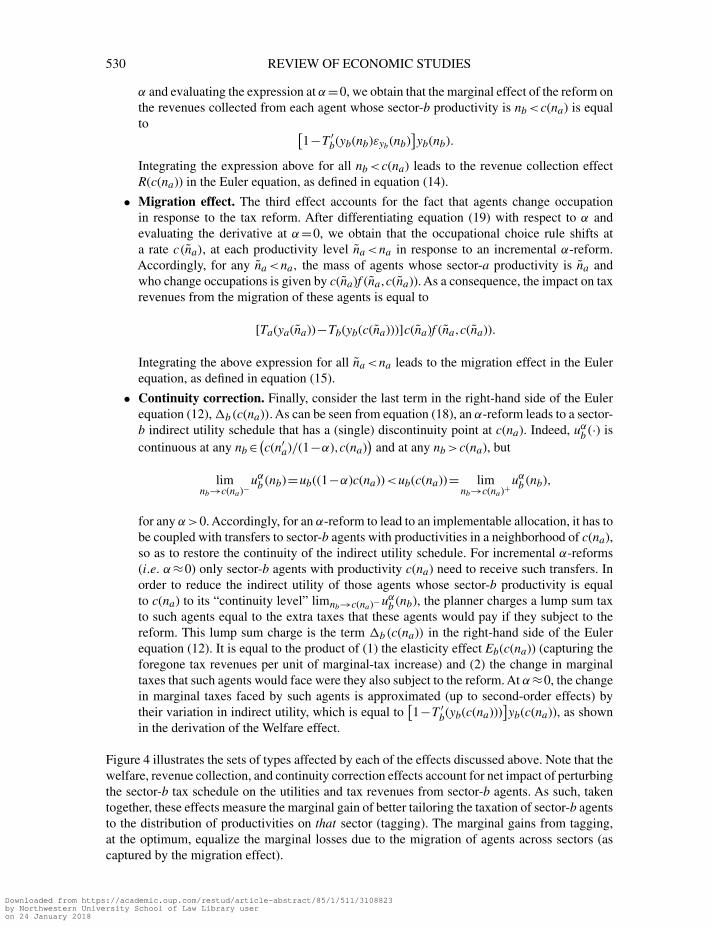
Figure 4 illustrates the sets of types affected by each of the effects discussed above. Note that thewelfare, revenue collection, and continuity correction effects account for net impact of perturbingthe sector-b tax schedule on the utilities and tax revenues from sector-b agents. As such, takentogether, these effects measure the marginal gain of better tailoring the taxation of sector-b agentsto the distribution of productivities on that sector (tagging). The marginal gains from tagging,at the optimum, equalize the marginal losses due to the migration of agents across sectors (ascaptured by the migration effect).
Downloaded from https://academic.oup.com/restud/article-abstract/85/1/511/3108823by Northwestern University School of Law Library useron 24 January 2018
[09:14 7/12/2017 rdx022.tex] RESTUD: The Review of Economic Studies Page: 531 511–557
GOMES ET AL. DIFFERENTIAL TAXATION AND OCCUPATIONAL CHOICE 531
Figure 4
The types affected by the welfare, revenue collection, migration, and continuity correction effects discussed
in the main text.
Note: The dotted curve corresponds the occupational choice rule under the α-payroll tax reform.
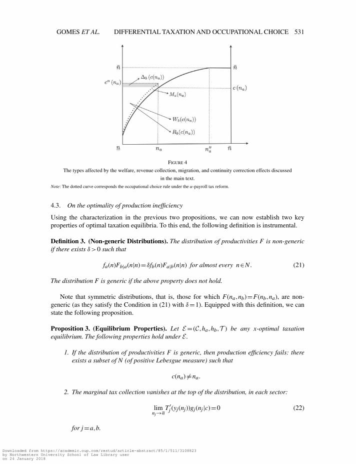
4.3. On the optimality of production inefficiency
Using the characterization in the previous two propositions, we can now establish two keyproperties of optimal taxation equilibria. To this end, the following definition is instrumental.
Definition 3. (Non-generic Distributions). The distribution of productivities F is non-genericif there exists δ>0 such that
fa(n)Fb|a(n|n)=δfb(n)Fa|b(n|n) for almost every n∈N . (21)
The distribution F is generic if the above property does not hold.
Note that symmetric distributions, that is, those for which F(na,nb)=F(nb,na), are non-generic (as they satisfy the Condition in (21) with δ=1). Equipped with this definition, we canstate the following proposition.
Proposition 3. (Equilibrium Properties). Let E = (C,ha,hb,T ) be any x-optimal taxationequilibrium. The following properties hold under E .
1. If the distribution of productivities F is generic, then production efficiency fails: thereexists a subset of N (of positive Lebesgue measure) such that
c(na) �=na.
2. The marginal tax collection vanishes at the top of the distribution, in each sector:
limnj→n
T ′j (yj(nj))gj(nj|c)=0 (22)
for j=a,b.
Downloaded from https://academic.oup.com/restud/article-abstract/85/1/511/3108823by Northwestern University School of Law Library useron 24 January 2018
[09:14 7/12/2017 rdx022.tex] RESTUD: The Review of Economic Studies Page: 532 511–557
532 REVIEW OF ECONOMIC STUDIES
Part 1 establishes that production inefficiency is a robust feature of optimal taxation equilibria.Intuitively, the densities fj(n)Fj|k(n|n), for j,k ∈{a,b} k �= j, capture the informational costs ofredistribution in the two sectors.24 Whenever such costs differ across the two sectors, the plannercan improve upon any equilibrium satisfying production efficiency by distorting occupationalchoice away from c(n)=n. Doing so yields a first-order reduction in the informational costs ofredistribution and only a second-order efficiency loss from the misallocation of talent across thetwo sectors (as the migration effect is zero under the efficient occupational choice rule). At theoptimum, the planner then distorts occupational choice up to the point where the marginal lossesin tax revenue due to the migration effect are equalized to the marginal gains from tailoring thetax schedule in each sector to the endogenous distribution of talent (tagging), as required by theEuler equation (12).25
Turning to Part 2, the result in the proposition says that, under any x-optimal taxationequilibrium, marginal tax collection vanishes at the top. This is either because top earners facevanishing marginal tax rates (which happens when the support of the productivity distribution isbounded, i.e. n<∞, and the density is bounded away from zero in a neighbourhood of (n,n)),or because the density of top earners vanishes (when n=∞, marginal taxes do not necessarilyvanish at the “top”, but equation (22) necessarily holds). The result thus extends familiar findingson the taxation of top earners (e.g. Mirrlees, 1971; Diamond and Mirrlees, 1971; Saez, 2002,among others) to the economy with multi-dimensional productivity and endogenous occupationalchoice under examination here. In particular, when n<∞, Proposition 3 reveals that distortionsin occupational choice do not translate into distortions in labour supply for those agents at thetop of the income distribution in each of the two sectors.
Before exploring the quantitative implications of the above characterization, we shall brieflydiscuss the case where sales taxes are the only instrument the government can employ todifferentiate taxes across sectors. As we shall see in Section 5, this exercise is useful to informpolicymakers on what percentage of the welfare gains from differential taxation can be obtainedby simple instruments such as sales taxes.
4.4. Sales taxes under uniform income taxation
The results above are developed under the assumption that the government can employ sector-specific income tax schedules. While this possibility appears plausible (e.g. business ownersface a different tax schedule than employees whose income comes through wages26), it is worthextending the above results to settings in which the government is unable to use sector-specificincome tax schedules, so that Ta =Tb. In this case, the tax treatment of the two sectors can differonly through the sales taxes τa and τb, which we now reintroduce (recall that these taxes play norole when income taxation is allowed to be sector-specific).
Consider an agent with type (na,nb) facing the tax system T ={T ,T ,τa,τb}, which featuresuniform income taxation. For this agent to be indifferent between working in one sector or theother, the maximal utility the agent can derive from working in either sector must be equalized,
24. These terms are the continuum-types analogs of the combination of the skill-transferability and and skill-intensity effects in the discrete type model of Section 2.
25. Note that when the c.d.f. F has full support over the type space [n,n]2, as assumed here, the continuum-typeanalog of the condition in Result 1 (namely, that there are low types sufficiently close to the 45-degree line) alwaysholds. In this sense, aside from knife-edge cases such as distributions F that are symmetric around the 45-degree line,the genericity condition in Definition 3 and the condition in Result 1 in the discrete-type model coincide.
26. See also the discussion in the “Introduction” about the use of sector-specific income taxation across countries.
Downloaded from https://academic.oup.com/restud/article-abstract/85/1/511/3108823by Northwestern University School of Law Library useron 24 January 2018
[09:14 7/12/2017 rdx022.tex] RESTUD: The Review of Economic Studies Page: 533 511–557
GOMES ET AL. DIFFERENTIAL TAXATION AND OCCUPATIONAL CHOICE 533
that is,
maxh
{(1−τa)hna −T ((1−τa)hna)−ψ(h)}=maxh
{(1−τb)hnb −T ((1−τb)hnb)−ψ(h)}
where we used the fact that wj =1−τj.As inspecting the problems above reveals, this occurs ifand only if (1−τa)na = (1−τb)nb. Therefore, whenever income taxation is uniform, the thresholdfunction is linear and given by27
c(na)= 1−τa
1−τbna. (23)
The converse is also true: whenever the occupational choice rule of an equilibrium E isdescribed by a linear threshold function, there exists a taxation equilibrium featuring uniformincome taxation that implements the same allocation as in E and yields the same utility to allagents. The reason is that, whenever the threshold function is linear (e.g. c(na)=κna), the effectivetax schedules must satisfy the relation
Ta(y)= (1−κ)y+Tb(κy),
as implied by the indifference condition ua(na)=ub(c(na)).28 Such effective taxes can begenerated, for example, by the tax system T ={Tb,Tb,1−κ,0}, which features uniform incometaxes.
The equivalence between linear threshold functions and uniform income taxes (with possiblydifferentiated sales taxes) greatly simplifies the task of finding the optimal tax system. Regardingthe primal problem Px
1 (C), Proposition 1 applies, as one only needs to set c(na) according toequation (23). In turn, to solve the dual problem Px
2 (ha), one only needs to maximize welfareover the linear coefficient that describes the threshold function. The result of this simple one-dimensional optimization problem is presented in the next proposition.
Proposition 4. (Occupational Choice: Sales Taxes). Suppose the government is constrained totax labour income homogeneously across sectors. The x-optimal tax system implementing thelabour supply schedule ha satisfies the following condition
limnb→n
{1CU
x ·Wb(nb)−Rb(nb)}= lim
na→n1−τb1−τa
Ma(na) (24)
where Wb, Rb, and Mb are, respectively, the welfare, the revenue collection, and the migrationeffects defined in Proposition 2, evaluated at the occupational choice rule (23).
The formula in equation (24) is closely related to the general Euler condition (12) ofProposition 2. The intuition for this formula can thus be obtained by considering α-payroll taxreforms similar to those considered above, but now applied to all individuals in sector b. The
27. Consistently with the analysis in the previous section, we continue to assume that sector a is the one for whichthere exists a n′′
a , such that c(na)= n, for all na ≥n′′a . This is equivalent to assuming that τa<τb.
28. Indeed, because c(na)=κna, it follows that, at any (na,κna)∈N,
maxh
{hna − Ta(hna)−ψ(h)
}=max
h
{hκna −Tb (hκna)−ψ(h)
}The right-hand side can be rewritten as maxh
{hna −
[(1−κ)hna +Tb (κhna)
]−ψ(h)
}, which implies the result.
Downloaded from https://academic.oup.com/restud/article-abstract/85/1/511/3108823by Northwestern University School of Law Library useron 24 January 2018
[09:14 7/12/2017 rdx022.tex] RESTUD: The Review of Economic Studies Page: 534 511–557
534 REVIEW OF ECONOMIC STUDIES
reason why the welfare, revenue collection, and migration effects must now be evaluated over allsector-b productivity levels is the limited flexibility of the government’s tax instruments underuniform income taxation. In particular, the fact that sales taxes impact uniformly all income levelsprecludes the possibility of restricting the α-payroll reform to a subset of the income levels insector b.As a result, equation (24) displays no continuity correction, given that any α-payroll-taxreform up to the highest income level generates no discontinuities in the schedule of indirectutilities.
As in the case of sector-specific income taxes, production efficiency generically fails under x-optimal taxation equilibria. Once again, the reason is that talent is not perfectly transferable acrosssectors. Therefore, a small departure from production efficiency typically generates first-ordergains in tax collection, while entailing only second-order losses in production. This contrastswith the Atkinson–Stiglitz theorem, according to which, when preferences over consumption andleisure are separable, as they are in our economy, the second-best can be implemented with zerosales taxes.
The x-optimal tax system under uniform income taxation is in general welfare-inferior to the x-optimal tax system with sector-specific income taxation. The next section assesses quantitativelythe magnitude of this discrepancy.
5. NUMERICAL ILLUSTRATION
In this section, we develop optimal policy simulations calibrated to the U.S. economy. Our goalis 3-fold. First, we quantitatively assess the welfare gains from sector-specific taxation relativeto a uniform tax system where production efficiency prevails. Secondly, we evaluate the welfareimpact from employing sector-specific income taxes relative to the case where only sales taxes(or, equivalently, payroll taxes) can differ across sectors, therefore assessing the welfare costsgenerated by simpler tax systems. Thirdly, we complement our analytical results by studying theincidence of production inefficiencies, and the shape of marginal and average tax schedules.
5.1. Constructing the distribution of skills
We use data from the Current Population Survey (CPS) on wages and industry classification.In line with the tax practices followed by many countries, we assign industries to either oneof the following two sectors: manufacturing and services. The manufacturing sector (indexedby a) comprises natural extraction, utilities, construction, transportation, and all manufacturingindustries. The services sector (indexed by b) comprises trade, the financial and bankingindustry, legal and business services, real state, arts, sports, and technology-intensive activitiescharacterized by large returns to occupation-specific skills. Because these sectors are large andheterogenous, our analysis produces a conservative estimate of the gains from sector-specifictaxation. A finer classification together with a more complex tax system can only magnify thewelfare effects discussed below.29
We interpret the wage data as generated by a (sub-optimal) uniform tax system whereproduction efficiency prevails. As such, each agent chooses the sector in which his productivityis the highest. We refer to this productivity as the effective productivity of an agent. We follow theliterature in assuming a constant wage elasticity of labour supply equal to 0.25. We then employstandard methods (as in Saez, 2001) to obtain the distribution of effective productivities using asinputs (1) the workers’ earnings data, and (2) the U.S. schedule of marginal tax rates. We denote
29. For further details on the data and the definition of sectors, see the Supplementary Material.
Downloaded from https://academic.oup.com/restud/article-abstract/85/1/511/3108823by Northwestern University School of Law Library useron 24 January 2018

[09:14 7/12/2017 rdx022.tex] RESTUD: The Review of Economic Studies Page: 535 511–557
GOMES ET AL. DIFFERENTIAL TAXATION AND OCCUPATIONAL CHOICE 535
by G the estimated distribution of effective productivities. As sector affiliation is observed in thedata, we denote by τj(n) the fraction of agents with effective productivity n working on sector j.
Estimating the distribution of effective productivities in each sector is not enough to recoverthe bi-dimensional skill distribution F, which is needed for computing the optimal tax system.30
Crucially, we cannot directly estimate the distribution of each agent’s lowest productivity (whichwe call latent productivity), since we do not observe the earnings that an agent would haveobtained had he worked in the sector where his productivity is the lowest.
We deal with this problem by constructing alternative scenarios on how latent productivitiesare distributed. In this respect, notice that, for an agent with effective productivity n, his latentproductivity belongs to the support [n,n]. We then denote by Hk (·|n) the distribution of the latentproductivity in sector k conditional on the effective productivity in sector j �=k being equal ton. In our simulations, we discretize the support of productivities by imposing a uniform grid.Productivity levels are indexed in increasing order by ω∈�≡{1,...,|�|}. As such, n(ω) is theωth lowest productivity in the grid. For its flexibility, we use the binomial c.d.f. to parametrizethe conditional distributions of latent productivities. Accordingly, for any ω≤ ω,
Hk(n(ω)|n(ω)
)= ω∑i=1
(ω
i
)pj(ω)i(1−pj(ω))ω−i.
Because the expected value of a random variable distributed according to Hk(n(ω)|n(ω)
)equals
pj(ω)n(ω), the parameter pj(ω)∈[0,1] is a natural measure of the degree of skill transferability,as defined in the discrete example of Section 2. Specifically, pj(ω) is the (average) fraction ofthe effective productivity n(ω) that sector-j agents can transfer to sector k. When pj(ω) is closeto zero, sector-j agents are essentially unproductive as they move to sector k, and the opposite istrue when p(ω) is close to one.
We employ the structure above to construct four scenarios:
Scenario 1. (High skill Transferability). pj(ω)=0.9 for all ω∈� and j∈{a,b}.In Scenario 1, all agents in either sector retain 90% of their productive capacity as they
move away from the sector in which their productivity is the highest. This scenario thus capturesan economy similar to those considered by Diamond and Mirrlees, where skills are perfectlytransferable across sectors. In light of the Diamond and Mirrlees Theorem, under Scenario 1,one should expect sector-specific taxation to produce modest welfare gains relative to uniformtaxation.
Scenario 2. (Low skill Transferability). pj(ω)=0.1 for all ω∈� and j∈{a,b}.In Scenario 2, all agents in either sector lose 90% of their productive capacity as they move
away from the sector in which their productivity is the highest. This scenario thus capturesan economy similar to those studied in the tagging literature initiated by Akerlof (1978),where migration across “tags” is not feasible (which is equivalent to skills being perfectlyuntransferable). In this context, differential taxation is expected to improve significantly welfareonly when the skill intensity is sufficiently different across sectors (recall the discussion on theskill intensity motive from Result 2 in Section 2).
Scenario 3. (High–low skill Transferability). pj(ω)=0.9 if G(n(ω))<0.5, and pj(ω)=0.1otherwise, for j∈{a,b}.
30. This observation echoes the non-identification results of the Roy model discussed in Heckman and Honoré(1990).
Downloaded from https://academic.oup.com/restud/article-abstract/85/1/511/3108823by Northwestern University School of Law Library useron 24 January 2018
[09:14 7/12/2017 rdx022.tex] RESTUD: The Review of Economic Studies Page: 536 511–557
536 REVIEW OF ECONOMIC STUDIES
Figure 5
Average latent productivities in Scenario 4.
Notes: The dashed curve depicts the average latent productivity (in sector b) of an agent whose effective productivity is na . The thickcurve depicts the average latent productivity (in sector a) of an agent whose effective productivity is nb (thus mapping the Y -axis into theX-axis). The dotted line is the 45-degree line.
Inspired by Result 1 from the discrete-type example, Scenario 3 combines the two scenariosabove so as to illustrate the potential gains from production inefficiency. It makes the (arguably,extreme) assumption that low-ability agents have a degree of skill transferability 0.9, whilehigh-ability agents have a degree of skill transferability of 0.1 (with a discontinuous change atthe median-skill level). This scenario captures in a stark way an economy in which agents ofdifferent productivity face different degrees of skill transferability. In the parlance of Section 2,this is an economy in which the skill transferability motive calls for sector-specific taxation.
Scenario 4. (Smoothly Decreasing Skill Transferability). pj(ω)=αj −βj (ω−1) for all ω∈�and j∈{a,b}, where αa>αb and βa<βb.
In Scenario 4, skill transferability is heterogeneous across agents and across sectors. Inline with recent empirical evidence, we make the plausible assumption that the degree of skilltransferability smoothly declines with earnings (in which case the percentage losses on earningsdue to sectorial migration are the highest at the top of the income distribution).31 As the servicessector comprises industries with high returns to occupation-specific skills (such as banking,finance and business, and legal services), we assume that it exhibits the lowest degree of skilltransferability at the top, and the highest at the bottom of the income distribution. Accordingly,we let αa<αb and βa<βb.
Figure 5 describes for Scenario 4 the expected latent productivity as a function of effectiveproductivities (being therefore the continuum-type analog to Figure 1 in the Illustrative Exampleof Section 2). That sector b has a lower degree of skill transferability at the top than sector a isreflected in the fact that the thick curve is farther to the diagonal than the dashed curve for highvalues of nb. Conversely, that sector b has a greater degree of skill transferability at the bottom
31. For evidence of this point on the finance and banking sector, see Bell and Van Reenen (2014) and Denk (2015).More generally, the labour literature finds that the percentage wage losses from switching sectors are greatest for workerswith higher incomes (see e.g. Neal, 1995). This reflects the fact that larger incomes come with longer tenures, duringwhich workers accumulate sector-specific (typically untransferable) human capital.
Downloaded from https://academic.oup.com/restud/article-abstract/85/1/511/3108823by Northwestern University School of Law Library useron 24 January 2018
[09:14 7/12/2017 rdx022.tex] RESTUD: The Review of Economic Studies Page: 537 511–557
GOMES ET AL. DIFFERENTIAL TAXATION AND OCCUPATIONAL CHOICE 537
TABLE 1Welfare effects of optimal sector-specific taxation
Scenario 1 Scenario 2 Scenario 3 Scenario 4
Sector-specific income taxes (%) 0.96 0.76 1.98 1.42Sector-specific sales taxes (%) 0.40% 0.17 0.72 0.75Sales tax τb(τa ≡0) (%) 4.6 4.2 5.3 10.8
Notes: In the top two rows, the percentage welfare gains achieved by the optimal tax systemrelative to uniform taxation. In the bottom row, the optimal sales tax in sector b when incometaxes are uniform and τa is normalized to zero.
than sector a is reflected in the fact that the dashed curve is farther from the diagonal than thethick curve for low values of na.32
In light of the skill transferability motive from Section 2, we should expect the manufacturingsector to be favoured by the optimal tax system under Scenario 4.
Equipped with the conditional distributions of latent productivities, we can readily recover thebi-dimensional distribution F. Lettingωa,ωb ∈� and denoting by g the probability mass functionassociated with G, it follows that
F(n(ωa),n(ωb))= G(n(ωk))+ωj∑
i=ωk+1
Hk (n(ωk)|n(i))g(n(i))τj(n(i)),
where we choose indexes so that ωj ≡max{ωa,ωb} and ωk ≡min{ωa,ωb}. The formula abovedecomposes the probability F(n(ωa),n(ωb)) into two terms: the first term is the probability thatthe effective probability is less than n(ωk). The second term is the probability that an agent workson sector j, enjoys an effective probability between n(ωk) and n(ωj), and has a latent productivitysmaller than n(ωk). This decomposition allows us to express the c.d.f. F in terms of the c.d.f.’sG and {Ha(·|n),Hb(·|n)} at any productivity pair (n(ωa),n(ωb)). Employing the results from theprevious section, we use this distribution to compute the Ralwsian-optimal tax system. Underthis welfare objective, the percentage gains in welfare can be conveniently interpreted also aspercentage variations in total tax collection.
5.2. Results
The impact of sector-specific taxation on welfare is moderate when the degree of skilltransferability is high across all income levels in both sectors, as considered in Scenario 1. Inthe case where income tax schedules can differ across sectors, these gains amount to 0.96%, andto 0.40% when only sales taxes are sector-specific (see Table 1). The reason for such a limitedimpact is that the migration effect is large when the distribution of productivities F concentratesmost mass around the 45-degree line. As a result, the optimal differential tax schedules are closeto uniform. Scenario 1, therefore, supports the conclusions of the Diamond–Mirrlees theoremwhen skill transferability is imperfect but high.
The welfare gains from sector-specific taxation are even smaller in Scenario 2, where skilltransferability is low across all income levels in both sectors. In this scenario, the migrationeffect is small, and most welfare gains from differential taxation arise from the government’sability to tailor marginal taxes to the distributions of productivities (under production efficiency)
32. To have a sense of magnitudes, the degree of skill transferability is 90% (resp., 95%) in sector a (resp., b) forthe bottom effective skill, and 60% (resp., 45%) in sector a (resp., b) for the top effective skill.
Downloaded from https://academic.oup.com/restud/article-abstract/85/1/511/3108823by Northwestern University School of Law Library useron 24 January 2018
[09:14 7/12/2017 rdx022.tex] RESTUD: The Review of Economic Studies Page: 538 511–557
538 REVIEW OF ECONOMIC STUDIES
Figure 6
The optimal occupational choice rules in Scenario 4.
Note: The dashed line corresponds to the case where only sales taxes are sector-specific, and the thick curve to the case where incometaxes are sector-specific.
among agents in each sector. However, because we purposely considered two large sectors, thesedistributions are rather similar. In the parlance of Section 2, the skill intensity does not vary muchacross sectors.As a result, the gains from sectorial taxation are limited, and optimal taxes are closeto uniform.33 We conjecture that by expanding the number of sectors, the gains from differentialtaxation are likely to increase, as the shape of informational rents should differ across sectors.
Scenario 3, where skill transferability sharply decreases with income, exhibits the highestgains from sectorial taxation. When sector-specific income taxation is possible, the welfare gainsof moving from the existing tax code to the optimal one are close to 2%. Interestingly, onlyone-third of these gains are realized by sector-specific sales taxes. This highlights the importanceof non-linear instruments in tailoring marginal taxes to different income levels.
The last scenario is likely to be the most realistic, as skill transferability decreases smoothlywith income in both sectors (but more markedly in the services sector). In this scenario, differentialincome taxation yields welfare gains of 1.42%, whereas differential sales taxes of 0.75%. Theseresults indicate that “simplicity” is not costless: another 0.67 percentage point in welfare gainscould be obtained by employing income taxes that are sector-specific (therefore almost doublingthe welfare gains from sector-specific sales taxes).
In Scenario 4, the optimal tax system favours the manufacturing sector, as reflected by theoccupational choice rule being uniformly above the 45-degree line (and sales taxes satisfyingτb>τa) - see Figure 6.34 Moreover, most of the migration from services to manufacturing occurs atintermediate- or low-skill levels. This occurs because, at skills close to the top, latent productivitiesare so low (see Figure 5 for the schedule of average latent productivities) that few agents actuallymigrate (i.e. the area between the threshold function and the 45-degree line contains a small massof agents when nb is close to the top).
33. More precisely, the distribution of productivities (under uniform taxation) in the services sector is slightlymore right-skewed than that on manufacturing (see Supplementary Material for further details). This property impliesthe services sector is overtaxed (e.g. the optimal sales tax sets τb>τa).
34. Note that, conditional on the optimal tax schedule favouring sector a, the distributions of latent productivities insector a do not affect the optimal tax system (since no agent in manufacturing migrates to services). As such, the welfareresults from Table 1 and the tax schedules discussed below are robust to other choices of Ha(·|nb).
Downloaded from https://academic.oup.com/restud/article-abstract/85/1/511/3108823by Northwestern University School of Law Library useron 24 January 2018
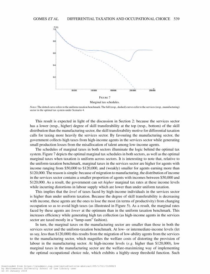
[09:14 7/12/2017 rdx022.tex] RESTUD: The Review of Economic Studies Page: 539 511–557
GOMES ET AL. DIFFERENTIAL TAXATION AND OCCUPATIONAL CHOICE 539
Figure 7
Marginal tax schedules.
Notes: The dotted curve refers to the uniform-taxation benchmark. The full (resp., dashed) curves refer to the services (resp., manufacturing)sector in the optimal tax system under Scenario 4.
This result is expected in light of the discussion in Section 2: because the services sectorhas a lower (resp., higher) degree of skill transferability at the top (resp., bottom) of the skilldistribution than the manufacturing sector, the skill transferability motive for differential taxationcalls for taxing more heavily the services sector. By favouring the manufacturing sector, thegovernment collects high taxes from high-income agents in the services sector while generatingsmall production losses from the misallocation of talent among low-income agents.
The schedules of marginal taxes in both sectors illuminate the logic behind the optimal taxsystem. Figure 7 depicts the optimal marginal tax schedules in both sectors, as well as the optimalmarginal taxes when taxation is uniform across sectors. It is interesting to note that, relative tothe uniform-taxation benchmark, marginal taxes in the services sector are higher for agents withincome ranging from $50,000 to $120,000, and (weakly) smaller for agents earning more than$120,000. The reason is simple: because of migration to manufacturing, the distribution of incomein the services sector contains a smaller proportion of agents with incomes between $50,000 and$120,000. As a result, the government can set higher marginal tax rates at these income levelswhile incurring distortions in labour supply which are lower than under uniform taxation.
This implies that the level of taxes faced by high-income individuals in the services sectoris higher than under uniform taxation. Because the degree of skill transferability is decreasingwith income, these agents are the ones to lose the most (in terms of productivity) from changingoccupation so as to avoid high taxes (as illustrated in Figure 5). As a result, the marginal ratesfaced by these agents are lower at the optimum than in the uniform taxation benchmark. Thisincreases efficiency while generating high tax collection (as high-income agents in the servicessector are taxed mostly in a “lump-sum” fashion).
In turn, the marginal taxes on the manufacturing sector are smaller than those in both theservices sector and the uniform-taxation benchmark. At low- or intermediate-income levels (letus say, less than $120,000) this results from the migration of low-ability agents from the servicesto the manufacturing sector, which magnifies the welfare costs of distorting the provision oflabour in the manufacturing sector. At high-income levels (e.g. higher than $120,000), lowmarginal taxes in the manufacturing sector are the welfare-maximizing way of implementingthe optimal occupational choice rule, which exhibits a highly-steep threshold function. Such
Downloaded from https://academic.oup.com/restud/article-abstract/85/1/511/3108823by Northwestern University School of Law Library useron 24 January 2018
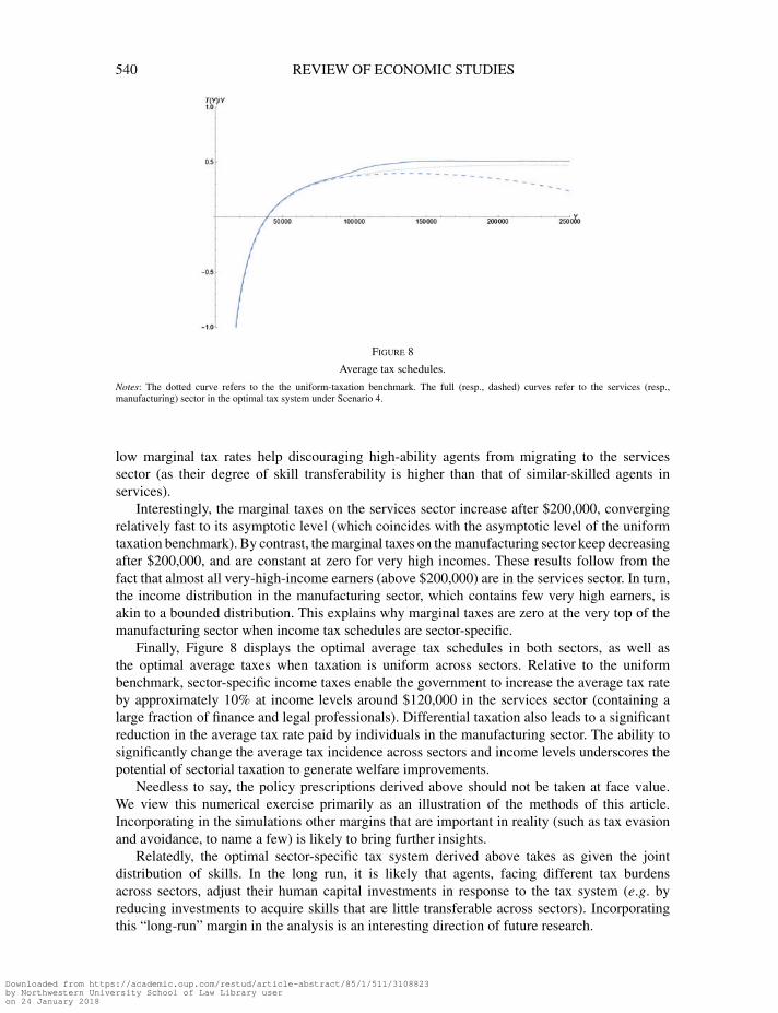
[09:14 7/12/2017 rdx022.tex] RESTUD: The Review of Economic Studies Page: 540 511–557
540 REVIEW OF ECONOMIC STUDIES
Figure 8
Average tax schedules.
Notes: The dotted curve refers to the the uniform-taxation benchmark. The full (resp., dashed) curves refer to the services (resp.,manufacturing) sector in the optimal tax system under Scenario 4.
low marginal tax rates help discouraging high-ability agents from migrating to the servicessector (as their degree of skill transferability is higher than that of similar-skilled agents inservices).
Interestingly, the marginal taxes on the services sector increase after $200,000, convergingrelatively fast to its asymptotic level (which coincides with the asymptotic level of the uniformtaxation benchmark). By contrast, the marginal taxes on the manufacturing sector keep decreasingafter $200,000, and are constant at zero for very high incomes. These results follow from thefact that almost all very-high-income earners (above $200,000) are in the services sector. In turn,the income distribution in the manufacturing sector, which contains few very high earners, isakin to a bounded distribution. This explains why marginal taxes are zero at the very top of themanufacturing sector when income tax schedules are sector-specific.
Finally, Figure 8 displays the optimal average tax schedules in both sectors, as well asthe optimal average taxes when taxation is uniform across sectors. Relative to the uniformbenchmark, sector-specific income taxes enable the government to increase the average tax rateby approximately 10% at income levels around $120,000 in the services sector (containing alarge fraction of finance and legal professionals). Differential taxation also leads to a significantreduction in the average tax rate paid by individuals in the manufacturing sector. The ability tosignificantly change the average tax incidence across sectors and income levels underscores thepotential of sectorial taxation to generate welfare improvements.
Needless to say, the policy prescriptions derived above should not be taken at face value.We view this numerical exercise primarily as an illustration of the methods of this article.Incorporating in the simulations other margins that are important in reality (such as tax evasionand avoidance, to name a few) is likely to bring further insights.
Relatedly, the optimal sector-specific tax system derived above takes as given the jointdistribution of skills. In the long run, it is likely that agents, facing different tax burdensacross sectors, adjust their human capital investments in response to the tax system (e.g. byreducing investments to acquire skills that are little transferable across sectors). Incorporatingthis “long-run” margin in the analysis is an interesting direction of future research.
Downloaded from https://academic.oup.com/restud/article-abstract/85/1/511/3108823by Northwestern University School of Law Library useron 24 January 2018
[09:14 7/12/2017 rdx022.tex] RESTUD: The Review of Economic Studies Page: 541 511–557
GOMES ET AL. DIFFERENTIAL TAXATION AND OCCUPATIONAL CHOICE 541
6. DISCUSSION AND CONCLUSIONS
Summary. This article studies differential taxation in a setting where workers’ skills are notperfectly transferable across sectors/occupations. We show how properties of optimal taxationequilibria can be identified by first considering a primal problem where the occupational choicerule (describing the allocation of agents across sectors) is held fixed, and where the governmentchooses a tax system to maximize welfare subject to implementing that occupational choice rule.Next, we consider a dual problem, where the labour supply of a given sector is held fixed, andwhere the government chooses a tax system, along with an occupational choice rule, to maximizewelfare subject to implementing that labour supply schedule.
The primal–dual approach described above generates a number of insights. First, it delivers ageneralized Mirrlees formula that determines how the government optimally balances intensive-margin distortions in labour supply across sectors, for any desired occupational choice rule.Secondly, it yields an Euler equation that summarizes all the trade-offs faced by the planner inchoosing the optimal occupational choice rule. The formula shows how, at the optimum, themarginal revenue losses from further distorting the allocation of workers across sectors (throughan increase in marginal taxes is some sectors) come from the dissipation of tax revenues due tothe migration of workers across sectors. The marginal gains, in turn, come from better tailoringthe tax schedule in each sector to its endogenous distribution of talent (tagging). These resultsimply failure of the Diamond–Mirrlees theorem: social welfare can be increased by inducingcertain agents to work in a sector in which their productivity is not the highest (i.e. productionefficiency is violated at the second-best).
We next quantify the welfare gains of differential taxation. First, we show that these gains canbe substantive under the empirically plausible assumption that the degree of skill transferabilityof agents decreases with income. Secondly, we show that “simpler” tax systems (involvinguniform income taxes but differential sales or payroll taxes) leave a sizable portion of thesegains unrealized. Thirdly, we document the incidence of production inefficiencies and the taxcollection gains that differential taxation generates from high earners in occupations with largewage premia.
k-sector extension. In the Supplementary Material, we extend the analysis to economies withk sectors. We show how the primal–dual approach described above can be extended to yielduseful formulas also in these richer settings. First, we show how the occupational choice rulecan be conveniently described by a collection of absolutely continuous and non-decreasingthreshold functions c≡ (cjl)j,l∈K,l �=j, one for each pair of sectors j,l, l �= j, such that an agentwith productivity type n= (n1,n2,...,nk)∈[n,n]k is induced to join sector j if, and only if, for alll �= j, nl<cjl(nj).
Next, we consider a primal problem analogous to the one in the two-sector model where theoccupational choice rule is held fixed and where the government maximizes welfare subject to abudget constraint, and to the requirement that the tax system implement the given occupationalchoice rule. The solution to this primal problem delivers a multi-sector generalization of theformula in Proposition 1 above.
We then proceed by solving a dual problem in which the labour supply in one sector isheld fixed and where the government maximizes welfare subject to the budget constraint andthe requirement that the resulting tax equilibrium be consistent with the labour supply schedulein that sector. The solution to this dual problem yields an Euler equation analogous to the onein Proposition 2. Interestingly, despite the complexity of the environment, these formulas areremarkably similar to those in the two-sector model. In particular, the Euler equation describingthe optimal occupational choice rule balances the same revenue collection, welfare, migration, and
Downloaded from https://academic.oup.com/restud/article-abstract/85/1/511/3108823by Northwestern University School of Law Library useron 24 January 2018

[09:14 7/12/2017 rdx022.tex] RESTUD: The Review of Economic Studies Page: 542 511–557
542 REVIEW OF ECONOMIC STUDIES
continuity correction effects as the simple formula in Proposition 2. It can be derived heuristicallyfrom the same type of α-payroll tax reforms considered above. However, migration in these richereconomies is more intriguing, for it involves migration from the sector in which the reform takesplace to each other sector in the economy. The key trick in solving such complex problems isa change in measure that permits one to express the endogenous talent distribution in all butone sector of the economy as a function of the talent distribution in the remaining sector. Aswe explain below, we expect these techniques will be useful also in other multi-dimensionalscreening problems. The k-sector model can also be fruitfully applied in quantitative exercisesthat extend the analysis of Section 5 to more than two sectors.
Other applications. Our analysis is conducted in the context of a multi-sector economy whereworkers choose their occupation by comparing their productivity differential across sectorswith the corresponding differential in the tax system. One alternative, and equally appealing,application of our results pertains to the design of tax systems in a federation of states. In thisapplication, the type of each worker describes his productivity in the different Member States.That a worker’s productivity varies across geographical areas may reflect technological, cultural,and linguistic differences across Member States. After observing the tax schedules and the wagesin each Member State, workers decide where to locate themselves, taking into account theirdifferences in productivities.35 The planner’s problem studied in this article (be it Ralwsian orconcave utilitarian) coincides with the problem of a federal authority designing the tax systemof each of its Member States so as to maximize aggregate welfare over the entire federation.Our results can then be directly applied to this problem and imply that differential tax treatmentsacross Member States are a robust feature of the optimal centralized tax system.36
Another application of the techniques developed in the present article pertains to the designof optimal tax systems in economies with a large informal sector. Economies plagued by a largedegree of informality in the labour market display a somewhat extreme form of differentialtaxation: workers in the formal sector face income taxes, while workers in the informal sector areable to evade such taxes. Yet, wages in both sectors are affected by sales taxes (and other formsof indirect taxation), which are typically easier to enforce than income taxes.37 The techniquesin Sections 4 and 4.4 above can be adapted to study the optimal combination of income and saletaxes in economies with an informal sector.38
The design of dual tax systems, where corporate and wage incomes are taxed differently,constitute yet another natural application of our results. Similar to the problem examined in thepresent article, the choice by many workers between employment and self-employment is oftenbased on the comparison between the productivity differential and the differential in the tax burdenacross the two regimes. More broadly, the study of the interplay between tax enforceability andoccupational choice, and its implications for the design of optimal tax systems, is a fascinatingtopic for future research.
35. See Kleven et al. (2013, 2014) and the references therein for empirical studies of how workers respond todifferential taxation by migrating from one state to another.
36. For models of competing tax authorities, see Hamilton and Pestieau (2005), and the references therein. In thesemodels, it is typically assumed that workers are (1) equally productive in the various member states, and (2) heterogenousin their mobility cost, which determines their location choice. In this setup, the centralized optimum always exhibitsproduction efficiency. By contrast, the richer heterogeneity considered in the present article reveals that differentialtaxation is a robust feature of centralized optimal tax systems.
37. Indeed, that sales taxes are easier to enforce than income taxes is widely recognized as a justification for theheavy reliance on such taxes (as well as other modes of indirect taxation) in underdeveloped economies.
38. See also Best et al. (2015) and the references therein for other examples of economies in which governmentsoptimally sacrifice production efficiency to boost tax revenues when their ability to enforce tax collection is limited.
Downloaded from https://academic.oup.com/restud/article-abstract/85/1/511/3108823by Northwestern University School of Law Library useron 24 January 2018
[09:14 7/12/2017 rdx022.tex] RESTUD: The Review of Economic Studies Page: 543 511–557
GOMES ET AL. DIFFERENTIAL TAXATION AND OCCUPATIONAL CHOICE 543
Finally, the techniques developed in this article can be applied to other multi-dimensionalscreening problems in which agents face rival choices. Consider first the application to nonlinearpricing by a multi-product monopolist with rival product lines (for instance, a car dealer designingprice–quality schedules for various car categories, such as sport and family cars). Given theirpreferences for each product line and the price-quality schedules offered by the seller, buyerschoose which type of car to buy, and then, select, within the chosen category, the desired model(identified by a combination of price and quality).39
Another application is the design of managerial compensation schemes with rival career paths.In this multi-dimensional extension, each manager chooses between different career paths as afunction of his productivity in each path and its respective performance-pay schedule. In designingthe remuneration in each career, the firm has to trade-off the profit losses from misallocatingmanagers across tasks with the reductions in informational rents that differential compensationschemes make possible.
Both the nonlinear pricing and the managerial compensation applications can be studied withthe primal–dual approach of this article. The solution to the primal and dual problems deliveranalogs of the generalized Mirrlees formula and the Euler equation, which can be used to deriveproperties of optimal contracts when agents face exclusive choices and have multi-dimensionalprivate information.
APPENDIX: OMITTED PROOFS
Proof of Lemma 1. Necessity. We first establish that, for the allocation (C,ha,hb) to be implemented at the wage ratesw by the tax system T , the properties in parts 1–3 must jointly hold. That wages must satisfy the condition in part (1) forthe labour market to clear follows directly from the fact that the production function exhibits constant returns to scale.
Next, consider the properties in part (2). For any j=a,b, let uj(y;nj)≡y−Tj(y)−ψ (y/(wjnj))
denote the utility thatan agent with sector-j productivity nj obtains from generating income y in sector j.Because the function satisfies the strictincreasing difference property, the correspondence yj(nj)=argmaxy
{y−Tj(y)−ψ (y/(wjnj)
)}must be non-decreasing
over N in the strong set order sense. Because N is compact, this means that yj(nj) is bounded over N . Next note thatuj(y;nj) is differentiable over N . Because yj(nj) is bounded over N, uj(y;nj) is equi-Lipschitz continuous over yj(N)×N ,with yj(N) denoting the range of yj(·). Standard envelope theorems (e.g. Milgrom and Segal, 2002) then imply that thevalue function
uj(nj)≡maxh
{wjhnj −Tj(wjhnj)−ψ(h)}=maxy
{uj(y;nj)}= maxy∈yj (N)
{uj(y;nj)}
must be Lipschitz continuous over N with derivative equal to
u′j(nj)=ψ ′
(yj(nj)
wjnj
)yj(nj)
wjn2j
for almost every nj ∈N , where yj :N → yj(N) is an arbitrary selection from the correspondence yj(·). Using the fact that,for any nj ∈Nj,
hj(nj)= yj(nj)
wjnj
along with the fact that uj(nj)= uj(nj) for all nj ∈Nj, we then have that the properties in part (2) are necessary.Finally, consider the properties in part (3). That the occupational choice rule C must satisfy these properties follows
directly from the fact that each uj(·) is Lipschitz continuous and strictly increasing over N along with the fact that the payoffuj(nj) that each agent obtains from joining each sector j and then choosing his labour supply optimally is independent ofhis productivity in any other sector.
Sufficiency. Now suppose that (C,ha,hb), along with the wage rates w and the tax system T , satisfies all the propertiesin parts 1–3 in the lemma. Then let T be any tax system such that, for all j=a,b, (a) τj =τj , (b) Tj(y)=Tj(y) for all
39. See Calzolari and Denicolò (2013, 2015) and Choné and Linnemer (2015) for recent contributions to theliterature on price discrimination under adverse selection and exclusive contracting.
Downloaded from https://academic.oup.com/restud/article-abstract/85/1/511/3108823by Northwestern University School of Law Library useron 24 January 2018

[09:14 7/12/2017 rdx022.tex] RESTUD: The Review of Economic Studies Page: 544 511–557
544 REVIEW OF ECONOMIC STUDIES
y such that y=wjnjhj(nj) for some nj ∈Nj, and (c) Tj(y)=Q∈R++ for all y such that there exists no nj ∈Nj such thaty=wjnjhj(nj). It is easy to see that there exists Q∈R++ large enough such that, for any j=a,b, any nj ∈N ,
argmaxy
{y−Tj(y)−ψ
(y
wjnj
)}⊂{
y :y=wjn′jhj(n
′j), n′
j ∈Nj
}.
That the allocation (C,ha,hb) is implemented at the wage rates w by the tax system T then follows from the followingfacts. Employing the effective labour
Lj =∫
{n:C(n)=j}hj(nj)njdF(n)
is profit maximizing for each firm j=a,b, given that the wages w satisfy the condition in part (1) and that the productionfunction exhibits constant returns to scale. For each type n joining sector j∈{a,b} (i.e. for which C(n)= j), the laboursupply hj(nj) satisfies the incentive compatibility condition on the intensive margin: uj(nj)= uj(nj). This follows from thefact that yj(nj)=wjhj(nj)nj is non-decreasing over Nj along with the fact that the equilibrium payoff satisfies the envelopecondition
uj(nj)=uj(n′j)+
∫ nj
n′j
ψ ′(hj(x)) hj(x)
xdx
for any pair nj,n′j ∈Nj and the fact that, for any y for which there exists no nj ∈Nj such that y=wjnjhj(nj), Tj(y)=Q.
Lastly, that the occupational choice rule C satisfies the incentive compatibility condition on the extensive marginfollows from the fact that, for any n any j∈{a,b} C(n)= j only if uj(nj)≥ ul(nl) all l �= j. This follows directly from thethreshold structure of C along with the fact that each uj(·) is strictly increasing, any j=a,b. ‖Proof of Remark 1. Under the original tax system T , wages are given by wj =1−τj . Faced with these wages, under the
original tax system, the optimal choice of effective labour h=nh for an agent with sector-j productivity nj who choosesto work in sector j is given by
argmaxh
{(1−τj)h−ψ(h/nj)−Tj
((1−τj)h
)}.
Under the new tax system T , wages are equal to wj =1, j=a,b, and the optimal choice of effective labour by the sameagent working in sector j is given by
argmaxh
{h−ψ(h/nj)−Tj(h)
}=argmax
h
{h−ψ(h/nj)−τj h−Tj
((1−τj)h
)}.
It is then easy to see that the original allocation (C,ha,hb) can be implemented under the wages Ow= (1,1) by the new taxsystem T . It is also easy to see that all agents’ payoffs (as well as the government’s tax income) under E are the same asunder E . ‖Proof of Proposition 1. First, note that, because ua and ub are Lipschitz continuous and strictly increasing, for almostevery na ∈N such that c(na)∈N , condition u′
a(na)=u′b(c(na))c′(na) must hold. Using Conditions (7) and (9), we then
have that, for almost every na ∈N such that (i) c(na)∈N and (ii) Ta(ya(na)) and Tb(yb(c(na))) are differentiable, Condition(11) must hold.
Let us now consider the government’s problem. It consists in choosing labour supply schedules ha :Na →R+, hb :Nb →R+ along with tax schedules Ta :R+ →R and Tb :R+ →R so as to maximize its x-objective:40
1CUx
∫Na
φ(ua(na))dGa(na|c)+1CUx
∫Nb
φ(ub(nb))dGb(nb|c)+[1−1CUx ]ua(n′
a),
whereuj(nj)=hj(nj)nj −ψ
(hj(nj)
)−Tj(njhj(nj)) for every nj ∈Nj , j=a,b
subject to (i) the budget constraint:∫Na
Ta(naha(na))dGa(na|c)+∫
Nb
Tb(nbhb(nb)))dGb(nb|c)≥B,
(ii) the labour supply incentive-compatibility constraints:
u′a(na)=ψ ′ (ha(na))
ha(na)
nafor almost every na ∈Na, (25)
40. Note that, in case of a Ralwsian objective, that is, for x=R, the lowest-utility agent is always an agent whosesector-a productivity is n′
a.
Downloaded from https://academic.oup.com/restud/article-abstract/85/1/511/3108823by Northwestern University School of Law Library useron 24 January 2018
[09:14 7/12/2017 rdx022.tex] RESTUD: The Review of Economic Studies Page: 545 511–557
GOMES ET AL. DIFFERENTIAL TAXATION AND OCCUPATIONAL CHOICE 545
u′b(nb)=ψ ′ (hb(nb))
hb(nb)
nbfor almost every nb ∈Nb, (26)
(iii) the occupational-choice incentive-compatibility constraints:41
hb(c(na))=Jc[na]ha(na), for all na ∈ (n′a,n
′′a), (27)
whereJc[na]≡
(c(na)/
(na ·c′(na)
))ξ,
and (iv) the monotonicity constraints:
yj(nj)=hj(nj)nj non-decreasing over Nj, j=a,b.
As mentioned in the main text, hereafter, we proceed by abstracting from the monotonicity constraints (iv), which isconsistent with the practice commonly followed in the literature.
Using the fact that (a) for any na ∈ (n′a,n),
Ta(naha(na)))=ha(na)na −ψ(ha(na))−ua(na),
along with the fact that (b) for nb ∈Nb, hb(nb)=Jc[c−1(nb)]ha(c−1(nb)) and ub(nb)=ua(c−1(nb)), it follows that
Tb(nbhb(nb))=hb(nb)nb −ψ(hb(nb))−ub(nb)
=Jc[c−1(nb)]ha(c−1(nb))nb −ψ(
Jc[c−1(nb)]ha(c−1(nb)))−ua(c−1(nb)).
Using the definition of the density
g(na|c)=ga(na|c)+c′ (na)gb(c(na)|c)
= fa(na)Fb|a(c(na)|na)+c′ (na)fb(c(na))Fa|b(na|c(na)),
we can then rewrite the government’s problem as that of choosing functions ua :Na →R, ha :Na →R+ so as to maximize∫Na
{1CU
x φ(ua(na))g(na|c)+[1−1CUx ]fa(na)ua(n′
a)}
dna (28)
subject to the budget constraint∫Na
{[ha(na)na −ψ(ha(na))−ua(na)]fa(na)Fb|a(c(na)|na)
}dna (29)
+∫
Na
{[Jc[na]ha(na)c(na)−ψ(Jc[na]ha(na))−ua(na)]c′(na)fb(c(na))Fa|b(na|c(na))
}dna,
≥B
and the IC constraints
u′a(n)=ψ ′ (ha(na))
ha(na)
nafor almost every na ∈Na.
This is a standard optimal control problem with control variable ha and state variable ua. The Hamiltonian associatedto this problem is:
H =1CUx φ(ua(na))g(na|c)+[1−1CU
x ]fa(na)ua(n′a)
+λ{[ha(na)na −ψ(ha(na))−ua(na)]fa(na)Fb|a(c(na)|na)}
+λ{Jc[na]ha(na)c(na)−ψ(Jc[na]ha(na))−ua(na)}c′(na)fb(c(na))Fa|b(na|c(na))
+μ(na)·ψ ′ (ha(na))ha(na)
na−λB,
where λ is the Lagrange multiplier associated to the common budget constraint (29) and where μ is the co-state variableassociated with the law of motion of ua. The transversality conditions are:
μ(n′a)=μ(n)=0. (30)
41. To see that the occupational choice incentive-compatibility constraint takes the form in equation (27), recallthat, for almost every na ∈N such that c(na)∈N , u′
a(na)=u′b(c(na))c′(na). Next, use equations (25) and (26), along with
the fact that ψ ′(h)=ξhξ−1, to arrive at equation (27).
Downloaded from https://academic.oup.com/restud/article-abstract/85/1/511/3108823by Northwestern University School of Law Library useron 24 January 2018
[09:14 7/12/2017 rdx022.tex] RESTUD: The Review of Economic Studies Page: 546 511–557
546 REVIEW OF ECONOMIC STUDIES
From the Pontryagin Maximum Principle,
μ′(na)=− ∂H
∂ua=[λ−1CU
x φ′(ua(na))]g(na|c). (31)
Integrating the right-hand side of equation (31) and using the transversality condition (30) we have that
μ(na)=−λ∫ n
na
[1−ma(na)1CU
x
]g(na|c)dna, (32)
where we used the definition of
ma(na)≡ φ′ (ua(na))
λ.
Furthermore, for any na such that ha (na)>0, the following first order condition must hold:
∂H
∂ha=λ[na −ψ ′ (ha(na))
]fa(na)Fb|a(c(na)|na)+
λ{Jc[na]c(na)−ψ ′ (Jc[na]ha(na))Jc[na]
}c′(na)fb(c(na))Fa|b(na|c(na))+
μ(na)ψ ′ (ha(na))+ψ ′′ (ha(na))ha(na)
na=0 (33)
Combining equations (32) with (33) and using the definitions of the densities
ga(na|c)= fa(na)Fb|a(c(na)|na) and gb(c(na)|c)= fb(c(na))Fa|b(na|c(na))
we obtain that: [na −ψ ′ (ha(na))
]ga(na|c)+{Jc[na]c(na)−ψ ′ (Jc[na]ha(na))Jc[na]
}c′(na)gb(c(na)|c) (34)
={ψ ′ (ha(na))+ψ ′′ (ha(na))ha(na)
na
}∫ n
na
[1−ma(na)1CU
x
]g(na|c)dna
Recall the first-order conditionnj −ψ ′(hj(nj)
)=T ′j (yj(nj))nj , j=a,b
and that
ψ ′ (ha(na))+ψ ′′ (ha(na))ha(na)
na= ψ ′ (ha(na))
na
{1+ ψ ′′ (ha(na))ha(na)
ψ ′ (ha(na))
}
=[1−T ′a(ya(na))
]ξ−1,
where ya(na)=naha(na). Hence, for any na>n′′a =c−1(n), the optimality condition (34) can be rewritten as the usual
Mirrlees condition
ξT ′
a(ya(na))
1−T ′a(ya(na))
nafa(na)=∫ n
na
[1−1CU
x ma(na)]fa(na)dna, (35)
where we also used the fact that, for na>c−1(n), ga(na|c)= fa(na). Next, consider any na ∈ (n′a,n
′′a). Using the fact that
Jc[na]ha(na)=hb(c(na)), equation (34) can be rewritten as
T ′a(ya(na))
1−T ′a(ya(na))
naga(na|c)+ T ′b(yb(c(na)))
1−T ′a(ya(na))
Jc[na]c′(na)c(na)gb(c(na)|c) (36)
=ξ−1∫ n
na
[1−ma(na)1CU
x
]g(na|c)dna.
Replacing equation (11) into (36) and using again the fact that Jc[na]ha(na)=hb(c(na)), we then have that, for anyna ∈ (n′
a,n′′a),
ξT ′
a(ya(na))
1−T ′a(ya(na))
naga(na|c)+ξ T ′b(yb(c(na)))
1−T ′b(yb(c(na)))
c(na)gb(c(na)|c) (37)
=∫ n
na
[1−1CU
x ma(na)]g(na|c)dna.
Combining the results establishes equation (10). ‖
Downloaded from https://academic.oup.com/restud/article-abstract/85/1/511/3108823by Northwestern University School of Law Library useron 24 January 2018
[09:14 7/12/2017 rdx022.tex] RESTUD: The Review of Economic Studies Page: 547 511–557
GOMES ET AL. DIFFERENTIAL TAXATION AND OCCUPATIONAL CHOICE 547
Proof of Proposition 2. Fix the sector-a labour supply schedule ha (with domain Na). The planner’s problem is asin the proof of Proposition 1, except that the control policies are now (i) the threshold function c :N → N defining theoccupational choice rule, with c continuous over N , strictly increasing over (n′
a,n′′a) for some n′′
a ≤ n, and such that c(na)=nfor all na ≤n′
a and c(na)= n for all na ≥n′′a, (ii) the sector-b labour supply schedule hb :Nb →R+, and the tax schedules
Tj :R+ →R, j=a,b.The planner’s problem can be conveniently rewritten by letting
Rxj
(nj)≡1CU
x φ(uj(nj))+λ{hj(nj)nj −ψ
(hj(nj)
)−uj(nj)}, (38)
denote the value the planner assigns to the utility of an agent whose sector-j productivity is nj , adjusted for the opportunitycost or raising funds from the agent, where λ is the multiplier associated with the government’s budget constraint. Theplanner’s problem can then be reformulated as consisting in choosing a threshold function c :N → N satisfying theproperties above, along with a sector-b labour supply schedule hb :Nb →R+, and a pair of utility functions ua :Na →R,ub :Nb →R that jointly maximize
∑j=a,b
n∫n
Rxj (n)gj(n|c)dn+[1−1CU
x ]ua(n′a) (39)
subject to the incentive compatibility constraints for labour supply
u′a(na)=ψ ′ (ha(na))
ha(na)
nafor almost every na ∈Na, (40)
u′b(nb)=ψ ′ (hb(nb))
hb(nb)
nbfor almost every nb ∈Nb, (41)
and the occupational choice constrainthb(c(na))=Jc[na]ha(na),
for all na ∈ (n′a,n
′′a) where n′′
a =c−1(n).Using the fact that, for any nb ∈ int(Nb),
hb(nb)=Jc[c−1(nb)]ha(c−1(nb)), (42)
andub(nb)=ua(c−1(nb)), (43)
along with the change in variables nb =c(na), we have that the planner’s objective can be rewritten as
n∫n′
a
[Rx
a (na)ga(na|c)+Rxb (na|c)gb(c(na)|c)c′(na)
]dna +[1−1CU
x ]ua(n′a) (44)
where, for any na ∈ (n′a,n
′′a),
Rxb (na|c)=Rx
b (c(na))
=1CUx φ(ub(c(na)))+λ{hb(c(na))c(na)−ψ(hb(c(na)))−ub (c(na))}
=1CUx φ(ua (na))+λ{Jc[na]ha(na)c(na)−ψ(Jc[na]ha(na))−ua (na)}
and Rxb (na|c)=0 if na ≥n′′
a .The planner’s problem can then be thought of as choosing (i) a scalar ua(n′
a), and (ii) an absolutely continuous functionc :N → N , strictly increasing over (n′
a,n′′a) for some 0≤n′
a and n′′a ≤ n and satisfying c(na)=0 if na ≤n′
a and c(na)= n ifna ≥n′′
a , so as to maximize equation (44). Given ua(n′a), because ha : (n′
a,n)→R+ is fixed, the function ua : (n′a,n)→R
is then uniquely determined by (40). The labour supply schedule hb :Nb →R+, and the utility schedule ub :Nb →R arethen given by equations (42) and (43), respectively. Finally, the tax schedules in the two sectors are given by
Tj(njhj(nj)))=hj(nj)nj −ψ(hj(nj)
)−uj(nj), j=a,b.
As a first step, let us fix the scalar ua(n′a)—and hence the entire utility function ua : (n′
a,n)→R—as well as thethresholds n′
a and n′′a and then look at the optimality conditions for the threshold function c : [n′
a,n′′a]→ N . To ease the
exposition, let Rxb :R3 →R be the function defined by
Rxb (na,c,J)≡1CU
x φ(ua (na))+λ{Jha(na)c−ψ(Jha(na))−ua (na)}, (45)
Downloaded from https://academic.oup.com/restud/article-abstract/85/1/511/3108823by Northwestern University School of Law Library useron 24 January 2018
[09:14 7/12/2017 rdx022.tex] RESTUD: The Review of Economic Studies Page: 548 511–557
548 REVIEW OF ECONOMIC STUDIES
and denote by ∂Rxb/∂na, ∂Rx
b/∂c, and ∂Rxb/∂J its partial derivatives. Then, for any na ∈[n′
a,n], let J :R3 →R be thefunction defined by
J(n,c,c′)=( c
nc′)ξ, (46)
and note that, for na ∈ (n′a,n
′′a), J(na,c(na),c′(na))=Jc[na]=
(c(na)/
(na ·c′(na)
))ξ. Hereafter, we then denote by Jn, Jc,
and Jc the partial derivatives of J with respect to n, c and c′, respectively. Finally, note that the densities
ga(na|c)≡ fa(na)Fb|a(c(na)|na)=∫ c(na)
nf (na,x)dx (47)
and
gb(c(na)|c)= fb(c(na))Fa|b(na|c(na))=∫ na
nf (x,c(na))dx (48)
depend on the entire function c only through the value that this function takes at na. In other words, ga(na|c) and gb(c(na)|c)can be thought of as functions of na, and c(na). This means that the optimality conditions for the threshold function c canbe obtained as a solution to a calculus of variations problem with control c and objective
n′′a∫
n′a
[Rx
a (na)ga(na|c)+Rxb
(na,c(na),J(na,c(na),c′(na))
)·c′(na)·gb(c(na)|c)]dna +[1−1CU
x ]ua(n′a).
Dropping the arguments from Rxb and J to facilitate the writing, we then have that, at any na ∈ (n′
a,n′′a), the point-wise
Euler equation of this problem is given by
Rxa (na)f (na,c(na))+ ∂Rx
b
∂cc′(na)gb(c(na)|c)+ ∂Rx
b
∂JJcc′(na)gb(c(na)|c)+Rx
bc′(na)∂
∂c[gb(c(na)|c)]
= d
dna
[∂Rx
b
∂JJc′ c′(na)gb(c(na)|c)+Rx
bgb(c(na)|c)
]. (49)
Use equation (48) to note that the fourth term of the left-hand-side of (49) can be developed as follows:
Rxbc′(na)
∂
∂c[gb(c(na)|c)]= Rx
bc′(na)
(∫ na
n
∂
∂nbf (x,c(na))dx
)
= Rxb
d
dna[gb(c(na)|c)]−Rx
bf (na,c(na))
= d
dna
[Rx
bgb(c(na)|c)]− dRx
b
dnagb(c(na)|c)−Rx
bf (na,c(na)). (50)
Substituting equation (50) into (49) and simplifying, we can rewrite the point-wise Euler equation (49) as follows
[Rx
a (na)−Rxb
]f (na,c(na))+ ∂Rx
b
∂cc′(na)gb(c(na)|c)+ ∂Rx
b
∂JJcgb(c(na)|c)c′(na)− dRx
b
dnagb(c(na)|c)
= d
dna
[∂Rx
b
∂JJc′ c′(na)gb(c(na)|c)
]. (51)
Multiplying both sides of equation (51) by c(na) and rearranging terms, we obtain that
[Rx
a (na)−Rxb
]f (na,c(na))c(na)+ ∂Rx
b
∂cc′(na)c(na)gb(c(na)|c)− dRx
b
dnac(na)gb(c(na)|c)
= d
dna
[∂Rx
b
∂JJc′ c′(na)gb(c(na)|c)
]c(na)− ∂Rx
b
∂JJcgb(c(na)|c)c(na)c′(na). (52)
Next, note that, for any na ∈ (n′a,n
′′a),
Jc =Jc(na,c(na),c′(na))=ξ(
c(na)
nac′(na)
)ξ−1 1
nac′(na)=ξJ
1
c(na),
Jc′ =Jc′ (na,c(na),c′(na))=−ξ(
c(na)
nac′(na)
)ξ−1 c(na)
nac′(na)
1
c′(na)=−ξJ
1
c′(na).
Note that the expressions above are always well-defined, as c′(na)>0 for all na ∈ (n′a,n
′′a) (by virtue of equation (11)).
Downloaded from https://academic.oup.com/restud/article-abstract/85/1/511/3108823by Northwestern University School of Law Library useron 24 January 2018
[09:14 7/12/2017 rdx022.tex] RESTUD: The Review of Economic Studies Page: 549 511–557
GOMES ET AL. DIFFERENTIAL TAXATION AND OCCUPATIONAL CHOICE 549
Replacing these expressions into the right-hand side of equation (52), we obtain that for any na ∈ (n′a,n
′′a), the
right-hand side of the Euler equation becomes
d
dna
[∂Rx
b
∂JJc′ c′(na)gb(c(na)|c)
]c(na)− ∂Rx
b
∂JJcgb(c(na)|c)c(na)c′(na)
=−ξ{
d
dna
[J∂Rx
b
∂Jgb(c(na)|c)
]c(na)+J
∂Rxb
∂Jgb(c(na)|c)c′(na)
}
=−ξ d
dna
[J∂Rx
b
∂Jgb(c(na)|c)c(na)
]. (53)
Substituting equation (53) into (52), we then have that, for any na ∈ (n′a,n
′′a), the Euler equation becomes
[Rx
a (na)−Rxb
]f (na,c(na))c(na)+ ∂Rx
b
∂cc′(na)c(na)gb(c(na)|c)− dRx
b
dnac(na)gb(c(na)|c)
=−ξ d
dna
[J∂Rx
b
∂Jgb(c(na)|c)c(na)
](54)
Integrating equation (54) from n′a to na ∈ (n′
a,n′′a) we then obtain that∫ na
n′a
[Rx
a (na)−Rxb(na)
]c(na)f (na,c(na))dna (55)
+∫ na
n′a
∂Rxb(na)
∂cc(na)c′(na)gb(c(na)|c)dna −
∫ na
n′a
dRxb(na)
dnac(na)gb(c(na)|c)dna
=−ξJ(na)∂Rx
b(na)
∂Jgb(c(na)|c)c(na)+ lim
na→n′a
ξJ(na)∂Rx
b(na)
∂Jgb(c(na)|c)c(na)
where we have highlighted the dependence of Rxb and of J on na to avoid possible confusion.
Consider the second term in the right-hand side of equation (55). This term is zero if n′a =n, as in this case
limna→n
gb(c(na)|c)= limna→n
fb(c(na))Fa|b(na|c(na))=0,
and all remaining terms are bounded. When n′a>n, the optimal choice of n′
a implies that the following transversalitycondition holds:
limna→n′
a
ξJ(na)∂Rx
b(na)
∂Jgb(c(na)|c)c(na)=0,
which is exactly the second term in the right-hand side of equation (55).We now express each term in equation (55) as a function of the income tax schedules. By definition of Rx
a (na) andRx
b(na) in equations (38) and (45), the first term in equation (55) is simply:∫ na
n′a
[Rx
a (na)−Rxb(na)
]c(na)f (na,c(na))dna
=λ∫ na
n′a
[Ta(ya(na))−Tb(yb(c(na)))]c(na)f (na,c(na))dna. (56)
The second term in equation (55) is obtained by differentiating equation (45) with respect to c, which yields
∫ na
n′a
∂Rxb(na)
∂cc(na)c′(na)gb(c(na)|c)dna =
∫ na
n′a
λJ(na)ha(na)c(na)c′(na)gb(c(na)|c)dna
=λ∫ na
n′a
yb(c(na))c′(na)gb(c(na)|c)dna =λ∫ c(na)
c(n′a)
yb(nb)gb(nb|c)dnb. (57)
where the last equality follows from changing the variable of integration from na to nb (using the relation nb =c(na)).
Downloaded from https://academic.oup.com/restud/article-abstract/85/1/511/3108823by Northwestern University School of Law Library useron 24 January 2018
[09:14 7/12/2017 rdx022.tex] RESTUD: The Review of Economic Studies Page: 550 511–557
550 REVIEW OF ECONOMIC STUDIES
The third term in equation (55) is obtained by totally differentiating equation (45) with respect to na, which gives∫ na
n′a
(dRx
b(na)
dnac(na)gb(c(na)|c)
)dna
=∫ na
n′a
{d
dna
[1CU
x φ(ua (na))+λTb(yb(c(na))]}
c(na)gb(c(na)|c)dna
=∫ na
n′a
{1CU
x φ′ (ua (na))u′a (na)+λT ′
b(yb(c(na))dyb(c(na))
dnbc′(na)
}c(na)gb(c(na)|c)dna
=∫ na
n′a
{1CU
x φ′ (ua (na))ψ′ (hb(c(na)))hb(c(na))
+λT ′b(yb(c(na)) dyb(c(na))
dnbc(na)
}c′(na)gb(c(na)|c)dna
=∫ na
n′a
{1CU
x φ′ (ua (na))[1−T ′
b(yb(c(na)))]yb(c(na))
+λT ′b(yb(c(na)) dyb(c(na))
dnbc(na)
}c′(na)gb(c(na)|c)dna
where the last two equalities use equations (9) and (11). Changing again the variables of integration using the relationnb =c(na), we then obtain that the third term in equation (55) is equal to∫ na
n′a
(dRx
b(na)
dnac(na)gb(c(na)|c)
)dna
=∫ c(na)
c(n′a)
{1CU
x φ′ (ub (nb))[1−T ′
b(yb(nb))]+λT ′
b(yb(nb))εyb (nb)}
yb(nb)gb(nb|c)dnb,
where
εyb (nb)≡ dyb(nb)
dnb
nb
yb(nb)
Finally, the right-hand-side in equation (55) is obtained by differentiating equation (45) with respect to J which yields
∂Rxb
∂J=λha(na)
[c(na)−ψ ′ (J(na)ha(na))
]=λha(na)c(na)T ′b(J(na)ha(na)c(na)).
We then have that the right-hand side in equation (55) can be rewritten as
−ξJ(na)∂Rx
b(na)
∂Jgb(c(na)|c)c(na)=−ξλyb(c(na))T ′
b(yb(c(na)))gb(c(na)|c)c(na)
=ξ T ′b(yb (c(na)))
1−T ′b(yb(c(na)))
c(na)gb(c(na)|c)·{(1−T ′b(yb(c(na))))yb(c(na)
}. (58)
Substituting equations (56)–(58) into (55) and rearranging, yields equation (12). ‖Proof of Proposition 3. The proof has two parts, each establishing the result in the corresponding part of the proposition.
Part 1. We establish the result by showing that, when the distribution is generic, a taxation equilibrium sustainingproduction efficiency (that is, inducing an efficient occupational choice) fails to satisfy the necessary optimality conditions,as implied by equation (12), over a positive measure set of types. To see this, first use equation (11) to observe that, inany equilibrium sustaining production efficiency, ha(n)=hb(n)=h(n) for all n∈N . Then use (9) and (11) to verify that,in any such equilibrium, Ta(y)=Tb(y)=T (y) and hence ua(n)=ub(n)=u(n) for all n∈N .
Next, observe that, for production efficiency to be optimal, the Euler equations in Proposition 2 must hold for eachsector. Using the symmetry properties described above, we can rewrite these equations, for any n∈N, as follows:
1CUx
∫ n
nm(n)
[1−T ′(y(n))
]y(n)dGb(n|c)=
∫ n
n
[1−T ′(y(n)εy(n)
]y(n)dGb(n|c) (59)
+ξT ′(y(n))y(n)ngb(n|c),
1CUx
∫ n
nm(n)
[1−T ′(y(n))
]y(n)dGa(n|c)=
∫ n
n
[1−T ′(y(n)εy(n)
]y(n)dGa(n|c) (60)
+ξT ′(y(n))y(n)nga(n|c),
Downloaded from https://academic.oup.com/restud/article-abstract/85/1/511/3108823by Northwestern University School of Law Library useron 24 January 2018

[09:14 7/12/2017 rdx022.tex] RESTUD: The Review of Economic Studies Page: 551 511–557
GOMES ET AL. DIFFERENTIAL TAXATION AND OCCUPATIONAL CHOICE 551
where we used the fact that n′a =n′
b =n (which also implies that ga(n|c)=gb(n|c)=0), along with the fact that, for alln∈N, c(n)=n, ma(n)=mb(n)=m(n), εya (n)=εyb (n)=εy(n) with
εy(n)≡ dy(n)
dn
n
y(n)and y(n)=nh(n).
Note that the Lagrange multiplier on the planner’s budget constraint is the same in both equations. The two Euler equations(59) and (60) define two linear differential equations in gb(n|c) and ga(n|c), respectively. Because the usual Lipschitzconditions hold (as implied by Lemma 1), the Picard–Lindelof theorem implies that each of these equations has a uniquesolution satisfying some associated boundary condition gj(n|c)= gj , for n>n. Because the differential equations defined
by (59) and (60) are homogenous, their solutions must satisfy gb(n|c)=δga(n|c) for δ= gbga.Because production efficiency
implies thatgb(n|c)= fb(n)Fa|b(n|n) and ga(n|c)= fa(n)Fb|a(n|n)
for all n∈N , we then conclude that, for production efficiency to be optimal, we have that for all n∈N
fb(n)Fa|b(n|n)=δfa(n)Fb|a(n|n).
As a consequence, for any generic F, any x-optimal taxation equilibrium entails production inefficiency for a positive-measure subset of types.
Part 2. Consider the calculus of variations problem described in the proof of Proposition 2 with objective function (44).The optimal choice of n′′
a implies that the following transversality condition holds:
limna→n′′
a
ξJ(na)∂Rx
b(na)
∂Jgb(c(na)|c)c(na)=0.
By the arguments in the proof of Proposition 2, this condition is equivalent to
0= limna→n′′
a
Eb(c(na))(1−T ′b(yb(c(na)))yb(c(na))= lim
nb→nnbyb(nb)T ′
b(yb(nb))gb(nb|c).
Because nbyb(nb) is strictly increasing and positive, it then follows that condition (22) has to hold for sector b. Finally, thatcondition (22) holds for sector a follows from the Mirrlees formula (10), after setting the indicator function to zero. ‖Proof of Proposition 4. Note that, with uniform labour income taxation and our convention about the labeling of the twosectors (which consists in assuming that τa ≤τb), n′
a =n. In deriving the optimality conditions below, for convenience wewill set the sale tax in sector b to τb =0. Once these conditions are identified, we will show how they can be expressedfor arbitrary combinations of τa and τb.
Following arguments similar to those in the proof of Proposition 2, the dual problem Px2 (ha) can be recast as consisting
in choosing a level of utility ua(n)≥0, along with a sale subsidy τa ≤0 so as to maximize∫ n1−τa
n1CU
x φ(ua(na))[ga(na|c)+(1−τa)gb((1−τa)na|c)]dna +∫ n
n1−τa
1CUx φ(ua(na))fa (na)dna
+[1−1CUx ]ua(n)
subject to the budget constraint∫ n1−τa
n[(1−τa)naha(na)−ψ(ha(na))−ua (na)][ga(na|c)+(1−τa)gb((1−τa)na|c)]dna+
∫ n
n1−τa
[(1−τa)ha(na)na −ψ(ha(na))−ua (na)]fa (na)dna +τa
∫ n
nnaha(na)ga(na|c)dna ≥B
where
ua(na)=ua(n)+na∫
n
ψ ′ (ha(na))ha(na)
nadna (61)
is determined by equation (9) and where the densities under the occupational choice rule corresponding to the sale tax τa
are given byga(na|c)= fa(na)Fb|a((1−τa)na)|na) (62)
andgb(nb|c)= fb(nb)Fa|b((1−τa)−1nb)|nb). (63a)
Downloaded from https://academic.oup.com/restud/article-abstract/85/1/511/3108823by Northwestern University School of Law Library useron 24 January 2018

[09:14 7/12/2017 rdx022.tex] RESTUD: The Review of Economic Studies Page: 552 511–557
552 REVIEW OF ECONOMIC STUDIES
Note that in writing the above program, we used the fact that, for any na ∈(
n, n1−τa
), (i) c(na)= (1−τa)na, (ii) hb(c(na))=
hb((1−τa)na)=ha(na), and (iii) yb(c(na))=c(na)hb(c(na))= (1−τa)naha(na).We also used the fact that, once ua(n) andτa are chosen, because ha is given, the common labour income tax schedule T is then given by
T ((1−τa)naha(na))= (1−τa)naha(na)−ψ(ha(na))−ua(na)
for all na ∈N . To put it differently, once ua(n) is chosen, different choices of the sale tax τa translate into different commonincome tax schedules T while leaving the sector-a effective tax schedule
Ta(ya(na))≡τaya(na)+T ((1−τa)ya(na))=ya(na)−ψ(
ya(na)
na
)−ua(na)
fixed, for any level of effective income y=ya(na)=naha(na), na ∈Na. This also means that the budget constraint in theabove program can be rewritten as∫ n
1−τa
n[naha(na)−ψ(ha(na))−ua (na)]ga(na|c)dna +
∫ n
n1−τa
[naha(na)−ψ(ha(na))−ua (na)]fa(na)dna
+∫ n
1−τa
n[(1−τa)naha(na)−ψ(ha(na))−ua (na)](1−τa)gb((1−τa)na|c)dna ≥B
Then, for any na ∈Na let
Rxa (na)≡1CU
x φ(ua (na))+λ[ha (na)na −ψ(ha (na))−ua (na)], (64)
while for any na ∈(
n, n1−τa
)let
Rxb (na|c)≡Rx
b (c(na)) (65)
=1CUx φ(ub(c(na)))+λ{hb(c(na))c(na)−ψ(hb(c(na)))−ub (c(na))}
=1CUx φ(ua (na))+λ{Jc[na]ha(na)c(na)−ψ(Jc[na]ha(na))−ua (na)}
=1CUx φ(ua (na))+λ[ha (na)(1−τa)na −ψ(ha (na))−ua (na)],
where λ is the Lagrangian multiplier associated with the government’s budget constraint. The Lagrangian for the aboveprogram then becomes ∫ n
nRx
a (na)ga(na|c)dna +∫ n
1−τa
nRx
b (na|c)(1−τa)gb((1−τa)na|c)dna
+[1−1CUx ]ua(n)−λB
Fixing ua(n), we then have that the first order condition with respect to τa is
d
dτa
∫ n
nRx
a (na)ga(na|c)dna
+ d
dτa
∫ n1−τa
nRx
b (na|c)(1−τa)gb((1−τa)na|c)dna =0. (66)
The latter condition can be rewritten as
d
dτa
∫ n
nRx
a (na)ga(na|c)dna+ (67)
+ n
1−τaRx
b
(n
1−τa|c)
gb(n|c)
+∫ n
1−τa
nRx
b (na|c) d
dτa{(1−τa)gb((1−τa)na|c)}dna
+∫ n
1−τa
n
dRxb (na|c)dτa
(1−τa)gb((1−τa)na|c)dna =0.
Downloaded from https://academic.oup.com/restud/article-abstract/85/1/511/3108823by Northwestern University School of Law Library useron 24 January 2018

[09:14 7/12/2017 rdx022.tex] RESTUD: The Review of Economic Studies Page: 553 511–557
GOMES ET AL. DIFFERENTIAL TAXATION AND OCCUPATIONAL CHOICE 553
Consider the first term in equation (67) and note that it is equal to
d
dτa
∫ n
nRx
a (na)ga(na|c)dna = d
dτa
{∫ n1−τa
nRx
a (na)ga(na|c)dna +∫ n
n1−τa
Rxa (na)fa(na)dna
}(68)
=∫ n
1−τa
nRx
a (na)d
dτa[ga(na|c)]dna
=−∫ n
1−τa
nRx
a (na)naf (na,(1−τa)na)dna
where we used the fact that ga(na|c)= fa(na) for all na ≥ n1−τa along with equation (62).
Next, consider the third term in equation (67) and use equation (63a) to note that
d
dτa{(1−τa)gb((1−τa)na|c)}=− d
dna[nagb((1−τa)na|c)]+naf (na,(1−τa)na).
The the third term in equation (67) is thus equal to∫ n1−τa
nRx
b (na;c)d
dτa{(1−τa)gb((1−τa)na|c)}dna
=−∫ n
1−τa
nRx
b (na;c)d
dna[nagb((1−τa)na|c)]dna +
∫ n1−τa
nRx
b (na;c)naf (na,(1−τa)na)dna
Now observe that
−∫ n
1−τa
nRx
b (na;c)d
dna[nagb((1−τa)na|c)]dna
=−[Rx
b (na;c)nagb((1−τa)na|c)] n
1−τan
+∫ n
1−τa
n
d
dna
[Rx
b (na;c)]
nagb((1−τa)na|c)dna
=− limna→n
na
1−τaRx
b
(na
1−τa|c)
gb(na|c)
+∫ n
1−τa
n
{[1CU
x φ′ (ua(na))−λ]u′a (na)+λ
[h′
a (na)na (1−τa)+ha (na)(1−τa)−ψ ′ (ha (na))h′a (na)
]}··nagb((1−τa)na|c)dna
where the first equality follows from integration by parts, whereas the third equality follows from the fact that gb((1−τa)n|c)=0 along with the fact that
d
dna
[Rx
b (na;c)]=[1CU
x φ′ (ua(na))−λ]u′a (na)
+λ[h′a (na)na (1−τa)+ha (na)(1−τa)−ψ ′ (ha (na))h
′a (na)
].
We conclude that the third term in equation (67) is thus equal to∫ n1−τa
nRx
b (na;c)d
dτa{(1−τa)gb((1−τa)na|c)}dna (69)
=− limna→n
na
1−τaRx
b
(na
1−τa|c)
gb(na|c)
+∫ n
1−τa
n
{[1CU
x φ′ (ua(na))−λ]u′a (na)+λ
[h′
a (na)na (1−τa)+ha (na)(1−τa)−ψ ′ (ha (na))h′a (na)
]}··nagb((1−τa)na|c)dna
+∫ n
1−τa
nRx
b (na;c)naf (na,(1−τa)na)dna.
Downloaded from https://academic.oup.com/restud/article-abstract/85/1/511/3108823by Northwestern University School of Law Library useron 24 January 2018

[09:14 7/12/2017 rdx022.tex] RESTUD: The Review of Economic Studies Page: 554 511–557
554 REVIEW OF ECONOMIC STUDIES
Finally, consider the fourth term in equation (67). Differentiating equation (65) with respect to τa, we can show thatthis term is equal to
∫ n1−τa
n
dRxb (na;c)
dτa(1−τa)gb((1−τa)na|c)dna (70)
=−λ∫ n
1−τa
nha (na)na(1−τa)gb((1−τa)na|c)dna.
Substituting equations (68), (69), and (70) into (67) and simplifying, we obtain that the optimality condition can berewritten as
∫ n1−τa
n
{[1CU
x φ′ (ua(na))−λ]u′a (na)+λ
[h′
a (na)na (1−τa)−ψ ′ (ha (na))h′a (na)
]}· (71)
·nagb((1−τa)na|c)dna
=∫ n
1−τa
n
{Rx
a (na)−Rxb (na;c)
}naf (na,(1−τa)na)dna
Using the fact that
Rxa (na)−Rx
b (na;c)=λ[Ta(ya(na)−Tb(yb(c(na)))]we then have that equation (71) can be rewritten as
1CUx
∫ n1−τa
nma (na)u
′a (na)nagb((1−τa)na|c)dna (72)
+∫ n
1−τa
n
{−u′a (na)+h′
a (na)na (1−τa)−ψ ′ (ha (na))h′a (na)
}nagb((1−τa)na|c)dna
=∫ n
1−τa
n[Ta(ya(na)− Tb(yb(c(na)))]naf (na,(1−τa)na)dna
where we used the fact that ma (na)≡ φ′(ua(na))λ
.Using equation (9), we can then rewrite the first integral in equation (72) as follows:
1CUx
∫ n1−τa
n ma (na)u′a (na)nagb((1−τa)na|c)dna
=1CUx
∫ n1−τa
n ma (na)[1−T ′((1−τa)ya(na))
](1−τa)ya(na)gb((1−τa)na|c)dna
(73)
where ya(na)=naha(na) is the effective labour supply by an agent working in sector a with productivity na.
Likewise, we can rewrite the second integral in equation (72) as follows:
∫ n1−τa
n
{−u′a (na)+h′
a (na)na (1−τa)−ψ ′ (ha (na))h′a (na)
}nagb((1−τa)na|c)dna (74)
=∫ n
1−τa
n
{ −[1−T ′((1−τa)ya(na))](1−τa)ha(na)+h′
a (na)na (1−τa)−[1−T ′((1−τa)ya(na))
]na(1−τa)h′
a (na)
}·
·nagb((1−τa)na|c)dna
Using the fact that
y′(na)=ha(na)+h′a(na)na.
we can rewrite equation (74) as follows:
∫ n1−τa
n
{−1+T ′((1−τa)ya(na))
y′a (na)na
ya(na)
}(1−τa)ya(na)gb((1−τa)na|c)dna
Downloaded from https://academic.oup.com/restud/article-abstract/85/1/511/3108823by Northwestern University School of Law Library useron 24 January 2018
[09:14 7/12/2017 rdx022.tex] RESTUD: The Review of Economic Studies Page: 555 511–557
GOMES ET AL. DIFFERENTIAL TAXATION AND OCCUPATIONAL CHOICE 555
We conclude that equation (72) can be rewritten as
1CUx
∫ n1−τa
nma (na)
[1−T ′((1−τa)ya(na))
](1−τa)ya(na)gb((1−τa)na|c)dna (75)
=∫ n
1−τa
n
{1−T ′((1−τa)ya(na))
y′a (na)na
ya(na)
}(1−τa)ya(na)gb((1−τa)na|c)dna
+∫ n
1−τa
n[Ta(ya(na)− Tb(yb(c(na)))]naf (na,(1−τa)na)dna
Changing the variable of integration to nb = (1−τa)na, and multiplying both sides by (1−τa) we can then rewriteequation (75) as
1CUx
∫ n
n(1−τa)mb (nb)
[1−T ′(yb(nb))
]yb(nb)gb(nb|c)dnb (76)
=∫ n
n(1−τa)
{1−T ′(yb(nb))εyb (nb)
}yb(nb)gb(nb|c)dnb
+∫ n
1−τa
n[Ta(ya(na)−Tb(yb(c(na)))](1−τa)naf (na,(1−τa)na)dna
where we used the fact that, for any na ∈(
n, n1−τa
)
εyb (c(na))≡ y′b (c(na))c(na)
yb(c(na))= y′
a (na)na
ya(na)
Using the definition of “welfare effect”, “revenue collection effect”, and “migration effects” we have that equation (76)can be rewritten as
limnb→n
{1CU
x ·Wb (nb)−Rb (nb)}= lim
na→n1−τb1−τa
Ma (na),
where the functionals above are evaluated at the threshold function c(na)= (1−τa)na.Finally, after reintroducing τb by eliminating the normalization to τb =0, and replacing 1−τa
1−τb na for (1−τa)na, weobtain the formula in the proposition. ‖
Acknowledgments. For comments and useful suggestions, we thank the Editor, anonymous referees, and seminarparticipants at LAGV 2012 (Marseille), SED 2013 (Seoul), PET 2013 (Lisbon), PSE 2013 (Munich), Université deRennes, TTC 2014 (Köln), Warwick, University College London, Fundacao Getulio Vargas, Paris School of Economics,Southampton, the Federal Reserve Bank of Chicago, and IIESE Stockholm. We are also grateful to Pierre Bachas, GadiBarlevy, Marco Bassetto, Felix Bierbauer, Philippe Choné, Helmut Cremer, Guy Laroque, Etienne Lehmann, Vitor FarinhaLuz, Miltos Makris, Casey Rothschild and Florian Scheuer for their very helpful conversations, and to Laura Doval forexcellent research assistance. The usual disclaimer applies.
Supplementary Data
Supplementary data are available at Review of Economic Studies online.
REFERENCES
AKERLOF, G. (1978), “The Economics of ‘Tagging’ as Applied to the Optimal Income Tax, Welfare Programs andManpower Planning”, American Economic Review, 68, 8–19.
ALES, L., KURNAZ, M. and SLEET, C. (2015), “Technical Change, Wage Inequality, and Taxes”, American EconomicReview, 105, 3061–3101.
ATKINSON, A. and STIGLITZ, J. (1976), “The Design of the Tax Structure: Direct Versus Indirect Taxation”, Journalof Public Economics, 6, 55–75.
BAKIJA, J., COLE, A. and HEIM, B. T. (2012), “Jobs and Income Growth of Top Earners and the Causes of ChangingIncome Inequality: Evidence from US Tax Return Data” (Working Paper, Williams College).
BELL, B. and VAN REENEN, J. (2014), “Bankers and Their Bonuses”, Economic Journal, 124, F1–F21.BEST, M. A. BROCKMEYER, KLEVEN, H., SPINNEWIJN, J. and WASEEM, M. (2015), “Production vs Revenue
Efficiency with Limited Tax Capacity: Theory and Evidence from Pakistan”, Journal of Political Economy, 123,1311–1355.
Downloaded from https://academic.oup.com/restud/article-abstract/85/1/511/3108823by Northwestern University School of Law Library useron 24 January 2018
[09:14 7/12/2017 rdx022.tex] RESTUD: The Review of Economic Studies Page: 556 511–557
556 REVIEW OF ECONOMIC STUDIES
BLOOM, N., PRICE, D. J., GUVENEN, F., SONG, J. and von WACHTERK, T. (2016), “Firming Up Inequality” (WorkingPaper, University of Minnesota).
BOADWAY, R. (2012), “From Optimal Tax Theory to Tax Policy: Retrospective and Prospective Views” (The MunichLectures, MIT Press).
CALZOLARI, G. and DENICOLÒ, V. (2013), “Competition with Exclusive Contracts and Market-share Discounts”,American Economic Review, 103, 2384–2411.
CALZOLARI, G. and DENICOLÒ, V. (2015), “Exclusive Contracts and Market Dominance”, American EconomicReview, 3321–3351.
CHONÉ, P. and LAROQUE, G. (2010), “Negative Marginal Tax Rates and Heterogeneity”, American Economic Review,100, 2532–47.
CHONÉ, P. and LINNEMER, L. (2015), “Nonlinear Prices and Exclusion: I. Buyer Opportunism”, Rand Journal ofEconomics, 46, 217–240.
CREMER H., GAHVARI, F. and LOZACHMEUR, J.-M. (2010), “Tagging and Income Taxation: Theory and anApplication”, American Economic Journal: Economic Policy, 2, 31–50.
DENK, O. (2015), “Financial Sector Pay and Labour Income Inequality: Evidence From Europe”, (OECD EconomicsDepartment Working Papers, No. 1225, OECD Publishing, Paris).
DIAMOND, P. (1998), “Optimal Income Taxation:An Example with a U-shaped Pattern of Optimal Tax Rates”, AmericanEconomic Review, 88, 83–95.
DIAMOND, P. and MIRRLEES, J. (1971), “Optimal Taxation and Public Production 1: Production Efficiency”, AmericanEconomic Review, 61, 8–27.
GODECHOT, O. (2012), “Is Finance Responsible for the Rise in Wage Inequality in France?”, Socio-Economic Review,10, 447–470.
GOLOSOV M., TROSHKIN, M., TSYVINSKI,A. and WEINZIERL, M. (2013), “Preference Heterogeneity and OptimalCapital Income Taxation”, Journal of Public Economics, 97, 160–175.
GUVENEN, F. and KURUSCU, B. (2012), “Understanding the Evolution of the U.S. Wage Distribution: A TheoreticalAnalysis”, Journal of European Economic Association, 10, 482–517.
HAMMOND, P. (2000), “Reassessing the Diamond/Mirrlees Efficiency Theorem”, in Hammond, P. and Myles, G.(eds), Incentives, Organization, and Public Economics: Papers in Honour of Sir James Mirrlees (New York: OxfordUniversity Press).
HAMILTON, J. and PESTIEAU, P. (2005), “Optimal Income Taxation and the Ability Distribution: Implications forMigration Equilibria”, International Tax and Public Finance, 12, 29–45.
HECKMAN, J. and HONORÉ, B. (1990), “The Empirical Content of the Roy Model”, Econometrica, 42, 1121–1149.JACQUET, L. and LEHMANN, E. (2016), “Optimal Taxation with Heterogeneous Skills and Elasticities: Structural and
Sufficient Statistics Approaches” (Working Paper No 2016-04, Université de Cergy-Pontoise, France).KAPLAN S. N. and RAUH, J. (2010), “Wall Street and Main Street: What Contributes to the Rise in the Highest
Incomes?”, Review of Financial Studies, 23, 1004–1050.KLEVEN, H., LANDAIS, C., SAEZ, E. (2013), “Taxation and International Migration of Superstars: Evidence from the
European Football Market”, American Economic Review, 103, 1892–1924.KLEVEN, H., LANDAIS, C., SAEZ, E. and SCHULTZ, E. (2014), “Migration and Wage Effects of Taxing Top Earners:
Evidence from the Foreigners’ Tax Scheme in Denmark”, Quarterly Journal of Economics, 129, 333–378.MANKIW G. and WEINZIERL, M. (2010), “The Optimal Taxation of Height: A Case Study in Utilitarian Income
Redistribution”, American Economic Journal: Economic Policy, 2, 155–176.MAS-COLELL, A., WHINSTON, M. and GREEN, J. (1995), Microeconomic Theory (New York: Oxford University
Press).MILGROM, P. (2004), “Putting Auction Theory to Work” (Cambridge: Cambridge University Press).MILGROM, P. and SEGAL, I. (2002), “Envelope Theorems for Arbitrary Choice Sets”, Econometrica, 70, 583–601.MIRRLEES, J. (1971), “An Exploration in the Theory of Optimum Income Taxation”, Review of Economic Studies, 38,
175–208.NAITO, H. (1999), “Re-examination of Uniform Commodity Taxes Under Non-linear Income Tax System and its
Implication for Production Efficiency”, Journal of Public Economics, 71, 165–188.NEAL, D. (1995), “Industry-Specific Human Capital: Evidence from Displaced Workers”, Journal of Labor Economics,
13, 653–677.PHILIPPON, T. and RESHEF, A. (2012), “Wages and Human Capital in the US Finance Industry: 1909–2006”, Quarterly
Journal of Economics, 127, 1551–1609.ROCHET, J.-C. and CHONÉ, P. (1998), “Ironing, Sweeping and Multidimensional Screening”, Econometrica, 66,
783–826.ROY, A. (1951), “Some Thoughts on the Distribution of Earnings”, Oxford Economic Papers, 3, 135–146.SAEZ, E. (2001), “Using Elasticities to Derive Optimal Tax Rates”, Review of Economic Studies, 68, 205–229.SAEZ, E. (2002), “Optimal Income Transfer Programs: Intensive Versus Extensive Labor Supply Responses”, Quarterly
Journal of Economics, 117, 1039–1073.SAEZ, E. (2004), “Direct or Indirect Tax Instruments for Redistribution: Short-run Versus Long-run”, Journal of Public
Economics, 88, 503–518.ROTHSCHILD, C. and SCHEUER, F. (2013), “Redistributive Taxation in the Roy Model”, Quarterly Journal of
Economics, 128, 623–668.
Downloaded from https://academic.oup.com/restud/article-abstract/85/1/511/3108823by Northwestern University School of Law Library useron 24 January 2018

[09:14 7/12/2017 rdx022.tex] RESTUD: The Review of Economic Studies Page: 557 511–557
GOMES ET AL. DIFFERENTIAL TAXATION AND OCCUPATIONAL CHOICE 557
ROTHSCHILD, C. and SCHEUER, F. (2016), “Optimal taxation with Rent-Seeking”, Review of Economic Studies, 83,1225–1262.
SCHEUER, F. (2014), “Entrepreneurial Taxation with Endogenous Entry”, American Economic Journal: EconomicPolicy, 6, 126–163.
SCHEUER, F. and WERNING, I. (2016), “Mirrlees meets Diamond-Mirrlees: Simplifying Nonlinear Income Taxation”(Working Paper Stanford University).
Downloaded from https://academic.oup.com/restud/article-abstract/85/1/511/3108823by Northwestern University School of Law Library useron 24 January 2018


![Arnold and Commissioner of Taxation (Taxation) … and Commissioner of Taxation (Taxation) [2017] AATA 1318 PAGE 2 OF 26 CATCHWORDS TAXATION AND REVENUE – appeal …](https://img.pdfslide.us/doc/110x75/5af2c9387f8b9ac2469120bc/arnold-and-commissioner-of-taxation-taxation-and-commissioner-of-taxation.jpg)