Embed Size (px)
Citation preview
J Optim Theory Appl (2012) 153:436–460DOI 10.1007/s10957-011-9962-8
Differential Properties of the Symmetric Matrix-ValuedFischer-Burmeister Function
Liwei Zhang · Ning Zhang · Liping Pang
Received: 3 April 2011 / Accepted: 2 November 2011 / Published online: 22 November 2011© Springer Science+Business Media, LLC 2011
Abstract This paper focuses on the study of differential properties of the symmetricmatrix-valued Fischer–Burmeister (FB) function. As the main results, the formulasfor the directional derivative, the B-subdifferential and the generalized Jacobian ofthe symmetric matrix-valued Fischer–Burmeister function are established, which canbe utilized in designing implementable Newton-type algorithms for nonsmooth equa-tions involving the symmetric matrix-valued FB function.
Keywords Fischer–Burmeister function · Directional derivative · B-subdifferential ·Generalized Jacobian
1 Introduction
It is well known that NCP-functions serve to transform a complementarity probleminto a nonsmooth system of equations or into a unconstrained minimization problem.Among which, one of the most popular NCP-functions is the Fischer–Burmeister(FB) function. Active research has been done on the applications of the FB-functionin solving the nonlinear complementarity problems and the second-order cone com-plementarity problems. The symmetric matrix-valued FB-function also plays impor-tant roles in optimization problems over the cone of positive and definite symmetric
Communicated by Liqun Qi.
The authors are grateful to the anonymous referees for their helpful suggestions and commentsand thank Professor Shaohua Pan from South China University of Technology for helping us to proveProposition 4.1.
The work is Supported by the National Natural Science Foundation of China under projects No.11071029 and No. 11171049 and the Fundamental Research Funds for the Central Universities.
L. Zhang (�) · N. Zhang · L. PangSchool of Mathematical Sciences, Dalian University of Technology, Dalian, Chinae-mail: [email protected]
J Optim Theory Appl (2012) 153:436–460 437
matrices. It has many nice properties that could be utilized in algorithmic develop-ment for semidefinite complementarity problems and nonsmooth equations involvingthe semidefinite conic complementarity condition. It is known from [1] that the func-tion ΦFB is strongly semismooth; it plays a fundamental role in the analysis of thequadratic convergence of Newton-type methods for solving systems of nonsmoothequations involving the semidefinite conic complementarity condition; see [2] for in-stance. It is proved by [3] that the gradient mapping of the squared norm of ΦFB isLipschitz continuous. However, these properties are generally not enough to facilitatethe computations in Newton-type methods, and the study of the differential proper-ties of the symmetric matrix-valued FB-function is becoming the key in designingimplementable Newton-type algorithms.
This paper investigates the differential properties of the matrix-valued FB-function, including the formulas for the directional derivative, the B-subdifferential,and the generalized Jacobian.
The organization of the paper is as follows. In Sect. 2, we give some preliminariesabout first-order derivatives of symmetric matrix-valued mappings and perturbationtheory for eigenvalues and eigenvectors of symmetric matrices from [4] and [5], re-spectively. The formula for the directional derivative of ΦFB is established in Sect. 3.In Sect. 4, we develop the formulas for the B-subdifferential and the generalized Ja-cobian of ΦFB. Finally conclusions are given in Sect. 5.
2 Preliminaries
Let Sn denote the linear space of n × n real symmetric matrices endowed with the
inner product
〈X,Y 〉 := tr(XY), for any X,Y ∈ Sn,
where “tr” denotes the trace, i.e., the sum of the diagonal entries.The symmetric matrix-valued FB-function is the function ΦFB : S
n × Sn → S
n
defined by
ΦFB(X,Y ) = X + Y −√
X2 + Y 2, X,Y ∈ Sn, (1)
which is an extension to the scalar-valued FB-function [6] as follows:
φ(a, b) = a + b −√
a2 + b2, a, b ∈ R × R.
In [7], Tseng proves that
ΦFB(X,Y ) = 0 ⇐⇒ 0 � X ⊥ Y 0,
where the symbol ⊥ means “perpendicular under the inner product." For this rela-tionship, Kanzow and Nagel [8] suggest a proof somewhat different from the onegiven by Tseng [7].
Throughout this paper, we employ the following notations, which are rather stan-dard in matrix analysis. Concretely, for X ∈ S
n, X 0 (X � 0) means that X is asymmetric and positive semidefinite matrix (positive definite matrix). For any m × n
438 J Optim Theory Appl (2012) 153:436–460
matrix A and index sets I ⊆ {1,2, . . . ,m} and J ⊆ {1,2, . . . , n}, AIJ denotes thesubmatrix of A with rows and columns specified by I , J , respectively. Particularly,Aij is the entry of A at (i, j) position. We use “◦” to denote the Hardamard prod-uct between matrices, i.e., for any two m × n matrices A and B , the (i, j)-th entry ofC := A◦B is Cij = AijBij . For X,H ∈ S
n, define LX(H) by LX(H) := XH +HX.For any X ∈ S
n, we use λ1(X) ≥ λ2(X) ≥ · · · ≥ λn(X) to denote the real eigen-values of X (counting multiplicity) being arranged in the non-increasing order. Letλ(X) := (λ1(X),λ2(X), . . . , λn(X))T ∈ R
n. Let Λ(X) ∈ Sn be the diagonal matrix
whose i-th diagonal entry is given by λi(X), i = 1, . . . , n, i.e., Λ(X) = diag(λ(X)).Denote by On the set of all n × n orthogonal matrices in R
n×n and On(X) a subsetof On by
On(X) := {P ∈ On : X = PΛ(X)P T
}.
Let μ1 > · · · > μr be the distinct eigenvalues of X and denote αk := {i : λi(X) = μk}for k = 1, . . . , r . For each i ∈ {1, . . . , n}, we define li to be the number of eigenval-ues that are equal to λi(X) but are ranked before i (including i) and mi to be thenumber of eigenvalues that are equal to λi(X) but are ranked after i (excluding i),respectively, i.e., we define li and mi such that
λ1(X) ≥ · · · ≥ λi−li (X) > λi−li+1(X) = · · · = λi(X) = · · · = λi+mi(X)
> λi+mi+1(X) ≥ · · · ≥ λn(X).
Now we list some useful results about the symmetric matrices, which are neededin the subsequent discussions.
Lemma 2.1 [9, Lemma 2.1] For any n × n real matrices A,B and any Z ∈ Sn+, it
holds that
(A + B)T Z(A + B) � 2(AT ZA + BT ZB
),
(A − B)T Z(A − B) � 2(AT ZA + BT ZB
).
Lemma 2.2 [9, Lemma 2.2] Let X,Y ∈ Sn satisfy X2 +Y 2 � 0. Then, for any n×m
real matrices A,B ,
AT A + BT B − (AT X + BT Y
)(X2 + Y 2)−1
(XA + YB) 0.
For the analysis in next section, we apply Stewart theorem [5] to matrix per-turbation G + �G and zero eigenvalues of G, where G ∈ S
n+ and �G ∈ Sn are
n × n symmetric matrices. Let G = PDP T with D := Λ(G) and P ∈ On(G). Letα := {i : λi(G) > 0} and β := {i : λi(G) = 0}. For any �G ∈ S
n, denote
[Pα Pβ ]T �G[Pα Pβ ] :=[�Gαα �Gαβ
�GTαβ �Gββ
]
.
Define γ := ‖�Gαβ‖ and δ := mini∈α λi(G) − ‖�Gαα‖ − ‖�Gαβ‖.
J Optim Theory Appl (2012) 153:436–460 439
Lemma 2.3 If δ > 0 and γ ≤ δ/2, then there exists a matrix solution K of
K�Gαβ − (Dα + �Gββ)K = �GTαβ − K�GαβK (2)
such that ‖K‖ ≤ 2γ /δ; if, moreover, we set Pβ := (Pβ + PαK)(I + KT K)− 12 , then
the columns of Pβ form an orthonormal basis for Range Pβ which is an invariantsubspace of G + �G. The representation of G + �G on Pβ is
Dβ = (I + KT K
) 12 (�Gαα + �GαβK)
(I + KT K
)− 12 .
From the above lemma, we get a perturbation result about eigenvalues λi(G +�G) for i ∈ β , which plays a key role in developing the formula for the directionalderivatives whose proof is quite similar to that of [10, Proposition 1.4].
Proposition 2.1 Let i ∈ β . Then, for any small �G ∈ Sn, there exists a matrix K
satisfying (2) with ‖K‖ = O(‖�G‖), such that
λi(G + �G) = λli
(P T
β �GPβ − P Tβ �GPαD−1
α P Tα �GPβ
)+ O(‖�G‖3).
Lemma 2.4 [4, Proposition 2.2] Let Q be an orthogonal matrix in On such thatQT Λ(X)Q = Λ(X). Then we have
{Qαkαl
= 0, if k, l = 1, . . . , r, k �= l,
QαkαkQT
αk,αk= QT
αkαkQαk,αk
, if k = 1, . . . , r.(3)
From Lemma 2.4, we obtain that On(Λ(X)) = {Q ∈ On : Q satisfies (3)}.
Lemma 2.5 [4, Proposition 2.3] For any H ∈ Sn, let U be an orthogonal matrix such
that
UT(Λ(X) + H
)U = Λ
(Λ(X) + H
).
Then, for any H → 0, we have
⎧⎪⎪⎨
⎪⎪⎩
Uαkαl= O(‖H‖), if k, l = 1, . . . , r, k �= l,
UαkαkUT
αkαk= I|αk | + O(‖H‖2), if k = 1, . . . , r ,
dist(Uαkαk, O|αk |) = O(‖H‖2), if k = 1, . . . , r ,
and
λi
(Λ(X) + H
)− λi(X) − λli (Hαkαk) = O
(‖H‖2), i ∈ αk, k = 1, . . . , r.
Hence, for any given direction H ∈ Sn, the eigenvalue function λi(·) is directional
differentiable at X with λ′i (Λ(X);H) = λli (Hαkαk
), i ∈ αk , k = 1, . . . , r .
440 J Optim Theory Appl (2012) 153:436–460
For any given X ∈ Sn and each k ∈ {1, . . . , r}, there exists δk > 0 such that |μl −
μk| > δk , ∀ l �= k. Define a continuously scalar function gk(·) : R → R by
gk(t) =
⎧⎪⎪⎪⎪⎪⎨
⎪⎪⎪⎪⎪⎩
− 6δk
(t − μk − δk
2 ), if t ∈ (μk + δk
3 ,μk + δk
2 ],1, if t ∈ [μk − δk
3 ,μk + δk
3 ],6δk
(t − μk + δk
2 ), if t ∈ [μk − δk
2 ,μk − δk
3 ),
0, otherwise.
Let Pk(·) be the matrix-valued function with respect to gk(·), i.e., for any Y ∈ Sn,
Pk(Y ) = P diag(gk
(λ1(Y )
), . . . , gk
(λn(Y )
))P T ,
where P ∈ On(X).Define
F s(Y ) :=r∑
k=1
f (μk)Pk(Y ). (4)
Obviously, the function gk(·) is twice continuously differentiable at each μk , thefollowing result follows from [4].
Lemma 2.6 For each k = 1, . . . , r , Pk(·) is twice continuously differentiable at X.
For a real-valued function f : R → R, the associated matrix-valued function F :S
n → Sn is defined by
F(X) := P diag(f(λ1(X)
), . . . , f
(λn(X)
))P T . (5)
Let f [1](Λ(X)) ∈ Sn be the first divided difference matrix whose (i, j)-entry is given
by
f [1](Λ(X))ij
:=⎧⎨
⎩
f (λi (X))−f (λj (X))
λi (X)−λj (X), if i �= j = 1,2, . . . , n,
f ′(λi(X)), if i = j = 1, . . . , n.
The following result for the differentiability of the symmetric matrix functions F
defined in (5) can be found in [11] or [12].
Lemma 2.7 Let X ∈ Sn be given and have the eigenvalue decomposition X =
PΛ(X)P T . The symmetric matrix-valued function F is Fréchet differentiable at X,if and only if f is differentiable at λi(X). In this case, the Fréchet derivative of F(·)at X is given by
F ′(X)(H) = P[f [1](Λ(X)
) ◦ (P T HP)]
P T , ∀H ∈ Sn. (6)
Note that the formula (6) is independent of the choice of P and the ordering ofλ1(X), . . . , λn(X).
J Optim Theory Appl (2012) 153:436–460 441
3 Directional Derivative of ΦFB
To simplify the notation, we define a matrix-valued function � : Sn × S
n → Sn by
�(X,Y ) := X2 + Y 2.
Let G := �(X,Y ) and σ1 ≥ σ2 ≥ · · · ≥ σn be eigenvalues of G. Choose P ∈ On(G)
such that
G = PDP T , (7)
where D := diag(σ1, σ2, . . . , σn). Let f : R → R be the scalar function:
f (t) :={√
t, if t ≥ 0,√−t, if t < 0.
Define a mapping F : Sn → S
n+ as the matrix-valued function associated with thescalar function f , i.e.,
F(G) = P diag(f (σ1), f (σ2), . . . , f (σn)
)P T ,
it is obvious that F(G) = √G for G ∈ S
n+. Then we can rewrite ΦFB as
ΦFB(X,Y ) = X + Y − Ψ (X,Y ),
where Ψ is the compound function of F and �, i.e.,
Ψ (X,Y ) := (F • �)(X,Y ).
Let
D :=[Dα 00 0β
], (8)
where
α := {i : σi > 0} and β := {i : σi = 0}. (9)
We assume that μ1 > μ2 > · · · > μr > μr+1 = 0 are the distinct eigenvalues of G.Define the following subsets of {1, . . . , n}:
αk := {i : σi = μk}, k = 1, . . . , r + 1. (10)
Then {α1, . . . , αr+1} and {α1, . . . , αr} are partitions of {1, . . . , n} and α, respectively.Due to the strong semismoothness [1], ΦFB is directionally differentiable every-
where in Sn. Now, we characterize the directional derivative of ΦFB.
Proposition 3.1 For (X,Y ) ∈ Sn × S
n, let Z := [X Y ] ∈ Rn×2n, the matrix-valued
function ΦFB is directionally differentiable at (X,Y ) and the directional derivative,for any H := (HX,HY ) ∈ S
n × Sn is given by
442 J Optim Theory Appl (2012) 153:436–460
Φ ′FB
((X,Y ); (HX,HY )
)
= HX + HY − P
[f [1](D)αα ◦ P T
α LZ(H)Pα f [1](D)αβ ◦ P Tα LZ(H)Pβ
f [1](D)βα ◦ P Tβ LZ(H)Pα K(HX,HY )
]
P T ,
where
LZ(H) = LX(HX) + LY (HY ),
K(HX,HY ) = {P T
β
[(HX)2 + (HY )2]Pβ − P T
β LZ(H)PαD−1α P T
α LZ(H)Pβ
} 12 .
Proof For any (HX,HY ) ∈ Sn × S
n, let
�(t) : = ΦFB(X + tHX,Y + tHY ) − ΦFB(X,Y )
= t (HX + HY ) − [Ψ (X + tHX,Y + tHY ) − Ψ (X,Y )
]
= t (HX + HY ) − P(F(D + W(t)
)− F(D))P T ,
where
W(t) := t(
LX(HX) + LY (HY ))+ t2((HX)2 + (HY )2),
with
X := P T XP, Y := P T YP, HX := P T HXP and HY := P T HY P.
Let D(t) := D + W(t) admit the following spectral decomposition:
D(t) = U(t)diag(λ(D(t)
))U(t)T , U(t) ∈ On
(D(t)
).
Let Fn(D(t)) := F(D(t)) − F s(D(t)). Since F s(D) = F(D), we have
F(D(t)
)− F(D) = Fn(D(t)
)+ F s(D(t)
)− F s(D).
By Lemma 2.6, the mappings Pk(·), k = 1, . . . , r + 1 are twice continuously differ-entiable at D. Then we have
limt↓0
F s(D(t)) − F s(D)
t= lim
t↓0
∑r+1k=1 f (μk)(Pk(D(t)) − Pk(D))
t
=r+1∑
k=1
f (μk)P ′k(D)P T
(LX(HX) + LY (HY )
)P
=Ω1, (11)
where for k, l = 1, . . . , r + 1,
(Ω1)αkαl:=⎧⎨
⎩
1√μk+√
μlP T
αkLZ(H)Pαl
, if k �= l,
0αkαk, if k = l.
J Optim Theory Appl (2012) 153:436–460 443
For t sufficiently close to 0, we have Pk(D(t)) = ∑i∈αk
ui(t)ui(t)T , where ui(t)
is the ith column of the matrix U(t), k = 1, . . . , r + 1. Therefore, we can writeFn(D(t)) as
Fn(D(t)
)=r+1∑
k=1
∑
i∈αk
[f(λi
(D(t)
))− f (μk)]ui(t)ui(t)
T .
For each k = 1, . . . , r + 1, let
�k(t) :=∑
i∈αk
[f(λi
(D(t)
))− f (μk)]ui(t)ui(t)
T .
Noting that{
μk > 0, if k = 1, . . . , r ,
μk = 0, if k = r + 1,
we need consider the following two cases.
Case 1. Let k = 1, . . . , r and i ∈ αk . Since f is directionally differentiable at μk
and f ′(μk)(·) is positive homogeneous, we have
f(λi
(D(t)
))− f (μk) = f ′(μk)(λli
(W(t)αkαk
))+ O(t2).
Since ui(t)ui(t)T is uniformly bounded, we obtain that
�k(t) =∑
i∈αk
f ′(μk)(λli
(W(t)αkαk
))ui(t)ui(t)
T + O(t2).
By Lemma 2.5, we know that there exists Q(t)αkαk∈ O|αk | such that for any i ∈ αk ,
ui(t) =⎡
⎢⎣
O(‖W(t)‖)qi(t)
O(‖W(t)‖)
⎤
⎥⎦+ O
(‖W(t)‖2)=⎡
⎢⎣
O(t)
qi(t)
O(t)
⎤
⎥⎦+ O
(t2),
where qi(t) is the ith column of Q(t)αkαk. Since the eigenvalue function λi(·) is
locally Lipschitz continuous, we obtain that
λli
(W(t)αkαk
) = λli
((LX(tHX) + LY (tHY ) + (tHX)2 + (tHY )2)
αkαk
)
= λli
((LX(tHX) + LY (tHY )
)αkαk
)+ O(t2)
= tλli
(P T
αkLZ(H)Pαk
)+ O(t2),
which implies
�k(t) =⎡
⎢⎣
0 0 0
0∑
i∈αkf ′(μk)(λli (tP
Tαk
LZ(H)Pαk))qi(t)qi(t)
T 0
0 0 0
⎤
⎥⎦+ O
(t2).
444 J Optim Theory Appl (2012) 153:436–460
On the other hand, by the spectral decomposition of D(t) and Lemma 2.5, we get
Λαk
(D(t)
) = U(t)Tαk
(D + W(t)
)U(t)αk
= μkI|αk | + U(t)TαkαkW(t)αkαk
U(t)αkαk+ O
(t2)
= μkI|αk | +(Q(t)Tαkαk
+ O(‖W(t)‖2))W(t)αkαk
(Q(t)αkαk
+ O(‖W(t)‖2))+ O
(t2)
= μkI|αk | + tQ(t)Tαkαk
(P T
αkLZ(H)Pαk
)Q(t)αkαk
+ O(t2).
This, together with the fact that
Λαk
(D(t)
)− μkI|αk | = tΛ(P T
αkLZ(H)Pαk
)+ O(t2),
implies that
tΛ(P T
αkLZ(H)Pαk
)= tQ(t)Tαkαk
(P T
αkLZ(H)Pαk
)Q(t)αkαk
+ O(‖W(t)‖2).
Therefore,∑
i∈αk
tλli
(P T
αkLZ(H)Pαk
)qi(t)qi(t)
T
= tQ(t)αkαkΛ(P T
αkLZ(H)Pαk
)Q(t)Tαkαk
+ O(t2)
= tP Tαk
LZ(H)Pαk+ O
(t2),
and in turn,
�k(t) = 1
2√
μk
⎡
⎢⎣
0 0 0
0 tP Tαk
LZ(H)Pαk+ O(t2) 0
0 0 0
⎤
⎥⎦+ O
(t2)
= 1
2√
μk
⎡
⎢⎣
0 0 0
0 tP Tαk
LZ(H)Pαk0
0 0 0
⎤
⎥⎦+ O
(t2). (12)
Then, for any k ∈ {1,2, . . . , r}, we have
limt↓0
�k(t)
t= 1
2√
μk
⎡
⎢⎣
0 0 0
0 P Tαk
LZ(H)Pαk0
0 0 0
⎤
⎥⎦ (13)
Case 2. Suppose that k = r + 1, or equivalently αk = β , then
�r+1(W(t)
) =∑
i∈β
[f(λi
(D(t)
))− f (μk)]ui(t)ui(t)
T
J Optim Theory Appl (2012) 153:436–460 445
=∑
i∈β
f(λi
(D(t)
))ui(t)ui(t)
T .
By Proposition 2.1, we have
λi
(D(t)
)= λli
(W(t)ββ − W(t)βαD−1
α W(t)αβ
)+ O(‖W(t)‖3).
Define
Eββ(t) := W(t)ββ − W(t)βαD−1α W(t)αβ
and
Eββ(HX,HY ) := P Tβ
[(HX)2 + (HY )2]Pβ − P T
β LZ(H)PαD−1α P T
α LZ(H)Pβ,
then
Eββ(t) = t2Eββ(HX,HY ) + O(‖W(t)‖3).
In the remainder of the proof, we use Eββ instead of Eββ(HX,HY ), for notationsimplicity.
Partition ui(t) as ui(t) = [uαi (t) u
βi (t)]T . The spectral decomposition of D(t) im-
plies(D + W(t)
)ui(t) = λi
(D(t)
)ui(t),
from which we get
[W(t)ββ W(t)βα
W(t)αβ Dα + W(t)αα
][u
βi (t)
uαi (t)
]
= λi
(D(t)
)[u
βi (t)
uαi (t)
]
,
i.e.,⎧⎨
⎩
W(t)ββuβi (t) + W(t)βαuα
i (t) = λi(D(t))uβi (t),
W(t)αβuβi (t) + (Dα + W(t)αα)uα
i (t) = λi(D(t))uαi (t).
(14)
Noticing the nonsingularity of Dα , we have
uαi (t) = D−1
α
(λi
(D(t)
)uα
i (t) − W(t)ααuαi (t)
)− D−1α W(t)αβu
βi (t).
Then, by substituting the above equation into the first formula in (14), we have
W(t)ββuβi (t) − W(t)βαD−1
α W(t)αβuβi (t)
= λi
(D(t)
)u
βi (t) − W(t)βαD−1
α
(λi
(D(t)
)uα
i (t) − W(t)ααuαi (t)
).
Together with the fact U(t)αβ = O(‖W(t)‖), we obtain that
U(t)TββE(t)ββU(t)ββ = Λβ
(D(t)
)+ O(‖W(t)‖3).
446 J Optim Theory Appl (2012) 153:436–460
From Lemma 2.5, we know that there exists Q(t)ββ ∈ O|β| such that
U(t)ββ = Q(t)ββ + O(‖W(t)‖2),
then(Q(t)Tββ + O
(‖W(t)‖2))Eββ(t)(Q(t)ββ + O
(‖W(t)‖2))
= Λβ
(D(t)
)+ O(‖W(t)‖3). (15)
Simple calculation yields that
Q(t)ββΛβ
(D(t)
)Q(t)Tββ = Eββ(t) + L
(W(t)
)with L
(W(t)
) := O(‖W(t)‖3).
Hence,
�r+1(W(t)
) =∑
i∈β
[f(λi
(D(t)
))]ui(t)ui(t)
T
=∑
i∈β
√λi
(D(t)
)qi(t)qi(t)
T + O(‖W(t)‖2)
=√
Eββ(t) + L(W(t)
)+ O(‖W(t)‖2).
Let P ∈ O|β|(Eββ), then
Eββ = P diag(λ(Eββ)
)P T ,
with λ1(Eββ) ≥ · · · ≥ λ|β|(Eββ). Let μ1 > μ2 > · · · > μr ′ > μr ′+1 = 0 be the dis-tinct eigenvalues of Eββ . Denote
D :=(
Dα′ 0
0 0|β ′|×|β ′|
),
where α′ :=⋃r ′k=1 α′
k and β ′ := α′r ′+1 with
α′k := {
i : λi(Eββ) = μk
}, k = 1, . . . , r ′ + 1. (16)
Then√
Mββ(t) −√
t2Eββ = P T(F(t2D(t) + O
(‖W(t)‖3))− F(t2D(t)
))P ,
where Mββ(t) := Eββ(t)+L(W(t)). Similar to the above estimating precess, we get
√Mββ(t) −
√t2Eββ =
[O(‖W(t)‖6) O(‖W(t)‖3)
O(‖W(t)‖3) O(‖W(t)‖3/2)
]
ββ
+ O(‖W(t)‖3)
=[
0α′α′ 0
0 O(t3/2)β ′β ′
]+ O
(t3),
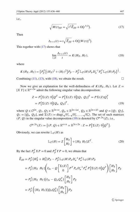
J Optim Theory Appl (2012) 153:436–460 447
i.e.,
√M(t)ββ =
√t2Eββ + O
(t3/2). (17)
Then
�r+1(t) = t
√Eββ + O
(‖W(t)‖2).
This together with (17) shows that
limt↓0
�r+1(t)
t= K(HX,HY ), (18)
where
K(HX,HY ) = {P T
β
[(HX)2 + (HY )2]Pβ − P T
β LZ(H)PαD−1α P T
α LZ(H)Pβ
} 12 .
Combining (11), (13), with (18), we obtain the result. �
Now we give an explanation for the well-definedness of K(HX,HY ). Let Z =[X Y ] ∈ R
n×2n admit the following singular value decomposition:
Z = P[�(Z) 0
]QT = P
[�(Z) 0
][Q1 Q2]T = P�(Z)QT1
= P[�(Z) 0
][Qα Qβ ]T , (19)
where Q ∈ O2n, Q1,Q2 ∈ R2n×n, Qα ∈ R
2n×|α|, Qβ ∈ R2n×|β| and Q = [Q1 Q2],
Q1 = [Qα Qβ ], and �(Z) := diag(√
σ1,√
σ2, . . . ,√
σn). The set of such matrices(P,Q) in the singular value decomposition (19) is denoted by On,2n(Z), i.e.,
On,2n(Z) := {(P,Q) ∈ R
n×n × R2n×2n : Z = P
[�(Z) 0
]QT
}.
Obviously, we can rewrite LZ(H) as
LZ(H) = Z
[HX
HY
]+ [HX HY ]ZT . (20)
By the fact P Tβ XP = 0 and P T
β YP = 0, we obtain that
Eββ = P Tβ
(H 2
X + H 2Y
)Pβ − P T
β LZ(H)PαD−1α P T
α LZ(H)Pβ
= P Tβ [HX HY ]
(
I2n − Q
[�(Z)
0
]P T PαD−1
α P Tα P
[�(Z) 0
]QT
)[HX
HY
]Pβ
= P Tβ [HX HY ](I2n − QαQT
α
)[HX
HY
]Pβ
= P Tβ
([HX HY ](QαQT
α
)[HX
HY
])Pβ
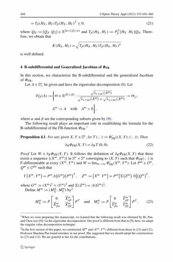
448 J Optim Theory Appl (2012) 153:436–460
= Tβ(HX,HY )Tβ(HX,HY )T 0, (21)
where Qα := [Qβ Q2] ∈ R2n×(|β|+n) and Tβ(HX,HY ) := P T
β [HX HY ]Qα . There-fore, we obtain that
K(HX,HY ) =√
Tβ(HX,HY )Tβ(HX,HY )T
is well defined.
4 B-subdifferential and Generalized Jacobian of ΦFB
In this section, we characterize the B-subdifferential and the generalized Jacobianof ΦFB.
Let A ∈ Sn+ be given and have the eigenvalue decomposition (8). Let
Wβ(A) :={Θ ∈ R
|β|×|β| :√
λi+|α|(Am)√
λi+|α|(Am) +√λj+|α|(Am)
→ Θij ,
Am → A with Am � 0
},
where α and β are the corresponding subsets given by (9).The following result plays an important role in establishing the formula for the
B-subdifferential of the FB-function ΦFB.1
Proposition 4.1 For any given X,Y ∈ Sn, let Υ (·, ·) := Φ ′
FB((X,Y ); (·, ·)). Then
∂BΦFB(X,Y ) = ∂BΥ (0,0). (22)
Proof Let W ∈ ∂BΦFB(X,Y ). It follows the definition of ∂BΦFB(X,Y ) that thereexists a sequence {(Xm,Ym)} in S
n × Sn converging to (X,Y ) such that ΦFB(·, ·) is
F-differentiable at every (Xm,Ym) and W = limm→∞ Φ ′FB(Xm,Ym). Let P m ∈ On,
Qm ∈ O2n such that
�(Xm,Ym
)= P mΛ(Gm
)(P m
)T, Zm := [
Xm Ym]= P m
[�(Zm)
0](
Qm)T
,
where Gm := (Xm)2 + (Ym)2 and �(Zm) = Λ(Gm)12 .
Define Mm := (MmX ,Mm
Y ) by2
MmX := P
[0 Xm
αβ
Xmβα Xm
ββ
]
P T and MmY := P
[0 Y m
αβ
Ymβα Ym
ββ
]
P T , (23)
1When we were preparing this manuscript, we learned that the following result was obtained by Bi, Pan,and Chen (see [9]) via the eigenvalue decomposition. Our proof is different from that in [9]; here, we adoptthe singular value decomposition technique.2In the first version of this paper, we constructed Mm and (Xm,Ym) different from those in (23) and (32),Professor Shaohua Pan found mistakes in our proof, She suggested that we should adopt the constructionsin (23) and (32). We are grateful to her for the contributions.
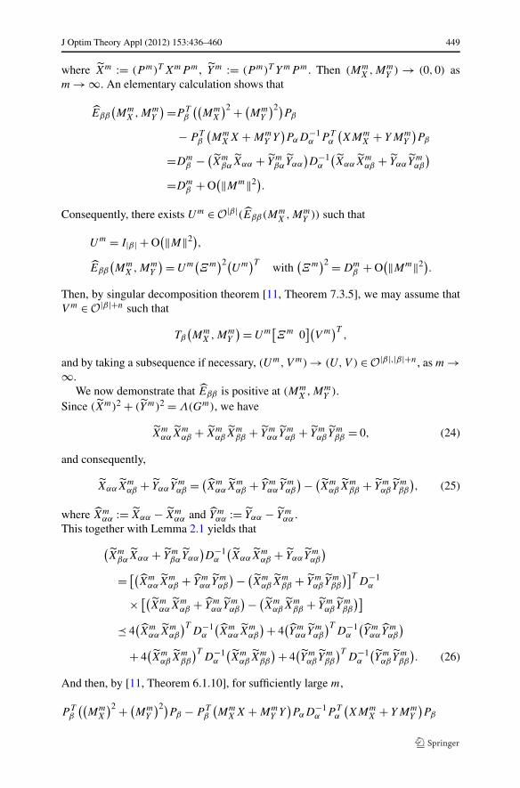
J Optim Theory Appl (2012) 153:436–460 449
where Xm := (P m)T XmP m, Y m := (P m)T YmP m. Then (MmX ,Mm
Y ) → (0,0) asm → ∞. An elementary calculation shows that
Eββ
(Mm
X ,MmY
)=P Tβ
((Mm
X
)2 + (Mm
Y
)2)Pβ
− P Tβ
(Mm
X X + MmY Y
)PαD−1
α P Tα
(XMm
X + YMmY
)Pβ
=Dmβ − (
XmβαXαα + Y m
βαYαα
)D−1
α
(XααXm
αβ + YααYmαβ
)
=Dmβ + O
(‖Mm‖2).
Consequently, there exists Um ∈ O|β|(Eββ(MmX ,Mm
Y )) such that
Um = I|β| + O(‖M‖2),
Eββ
(Mm
X ,MmY
)= Um(Ξm
)2(Um
)T with(Ξm
)2 = Dmβ + O
(‖Mm‖2).
Then, by singular decomposition theorem [11, Theorem 7.3.5], we may assume thatV m ∈ O|β|+n such that
Tβ
(Mm
X ,MmY
)= Um[Ξm 0
](V m
)T,
and by taking a subsequence if necessary, (Um,V m) → (U,V ) ∈ O|β|,|β|+n, as m →∞.
We now demonstrate that Eββ is positive at (MmX ,Mm
Y ).Since (Xm)2 + (Y m)2 = Λ(Gm), we have
XmααXm
αβ + XmαβXm
ββ + Y mααYm
αβ + Y mαβYm
ββ = 0, (24)
and consequently,
XααXmαβ + YααYm
αβ = (Xm
ααXmαβ + Y m
ααYmαβ
)− (Xm
αβXmββ + Y m
αβYmββ
), (25)
where Xmαα := Xαα − Xm
αα and Y mαα := Yαα − Y m
αα .This together with Lemma 2.1 yields that
(Xm
βαXαα + Y mβαYαα
)D−1
α
(XααXm
αβ + YααYmαβ
)
= [(Xm
ααXmαβ + Y m
ααYmαβ
)− (Xm
αβXmββ + Y m
αβYmββ
)]TD−1
α
× [(Xm
ααXmαβ + Y m
ααYmαβ
)− (Xm
αβXmββ + Y m
αβYmββ
)]
� 4(Xm
ααXmαβ
)TD−1
α
(Xm
ααXmαβ
)+ 4(Y m
ααYmαβ
)TD−1
α
(Y m
ααYmαβ
)
+ 4(Xm
αβXmββ
)TD−1
α
(Xm
αβXmββ
)+ 4(Y m
αβYmββ
)TD−1
α
(Y m
αβYmββ
). (26)
And then, by [11, Theorem 6.1.10], for sufficiently large m,
P Tβ
((Mm
X
)2 + (Mm
Y
)2)Pβ − P T
β
(Mm
XX + MmY Y
)PαD−1
α P Tα
(XMm
X + YMmY
)Pβ
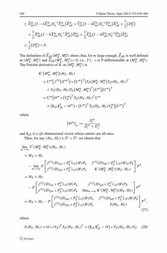
450 J Optim Theory Appl (2012) 153:436–460
Xmβα
(I − 4Xm
ααD−1α Xm
αα
)Xm
αβ + Y mβα
(I − 4Y m
ααD−1α Ym
αα
)Xm
αβ + 1
2
(Dm
β
)
+ 1
2Xm
ββ
(I − 8Xm
βαD−1α Xm
αβ
)Xm
ββ + 1
2Y m
ββ
(I − 8Y m
βαD−2α Ym
αβ
)Y m
ββ
1
2
(Dm
β
)� 0.
The definition of Eββ(MmX ,Mm
Y ) shows that, for m large enough, Eββ is well definedat (Mm
X ,MmY ) and Eββ(Mm
X ,MmY )� 0, i.e., Υ (·, ·) is F-differentiable at (Mm
X ,MmY ).
The Fréchet derivative of K at (MmX ,Mm
Y ) is
K ′(MmX,Mm
Y
)(HX,HY )
= Um[f [1](Ξm2) ◦ (Um
)T (Tβ
(Mm
X,MmY
)Tβ(HX,HY )T
+ Tβ(HX,HY )Tβ
(Mm
X,MmY
)T )Um
](Um
)T
= Um[Θm ◦ (V m
β
)TTβ(HX,HY )T Um
+ (1|β|1T|β| − Θm
) ◦ (Um)T
Tβ(HX,HY )V mβ
](Um
)T,
where
(Θm
)ij
:= Ξmi
Ξmi + Ξm
j
and 1|β| is a |β|-dimensional vector whose entries are all ones.Then, for any (HX,HY ) ∈ S
n × Sn, we obtain that
limm→∞Υ ′(Mm
X ,MmY )(HX,HY )
= HX + HY
− limm→∞P
[f [1](D)αα ◦ P T
α LZ(H)Pα f [1](D)αβ ◦ P Tα LZ(H)ZPβ
f [1](D)βα ◦ P Tβ LZ(H)Pα K ′(Mm
X ,MmY )(HX,HY )
]
P T
= HX + HY
− P
[f [1](D)αα ◦ P T
α LZ(H)Pα f [1](D)αβ ◦ P Tα LZ(H)Pβ
f [1](D)βα ◦ P Tβ LZ(H)Pα limm→∞ K ′(Mm
X ,MmY )(HX,HY )
]
P T
= HX + HY − P
[f [1](D)αα ◦ P T
α LZ(H)Pα f [1](D)αβ ◦ P Tα LZ(H)Pβ
f [1](D)βα ◦ P Tβ LZ(H)Pα S(HX,HY )
]
P T ,
(27)
where
S(HX,HY ) = Θ ◦ (Vβ)T Tβ(HX,HY )T + (1|β|1T|β| − Θ
) ◦ Tβ(HX,HY )Vβ (28)
J Optim Theory Appl (2012) 153:436–460 451
and Θ ∈ Wβ(G).
Again by singular decomposition theorem, we know that Qm := [Qmα Qm
α V m] satis-fies
[Xm Ym
]= P m[�(Zm)
0]Qm.
Define Q := [Qα QαV ], then
limm→∞
(P m,Qm
)= (P, Q).
For any H := (HX,HY ) ∈ Sn × S
n, we have
limm→∞Φ ′
FB(Xm,Ym)(HX,HY )
= HX + HY − limm→∞P m
[f [1](Λ(Gm)
) ◦ (P m)T (LXm(HX)
+ LYm(HY ))P m
](P m
)T
= HX + HY
− P
[f [1](Λ(G))αα ◦ P T
α LZ(H)Pα f [1](Λ(G))αβ ◦ P Tα LZ(H)Pβ
f [1](Λ(G))βα ◦ P Tβ LZ(H)Pα lim
m→∞f [1](Λ(Gm))ββ ◦ (P mβ )T LZm(H)P m
β
]
P T
(29)
and
limm→∞f [1](Λ
(Gm
))ββ
◦ (P mβ
)TLZm(H)P m
β
= limm→∞f [1](Λ
(Gm
))ββ
◦ (P mβ
)T (LXm(HX) + LYm(HY ))P m
β
= limm→∞f [1](Λ
(Gm
))ββ
◦ (P mβ
)T(
P m[f(Λ(Gm
))0](
Qm)T[HX
HY
]
+ [HX HY ]Qm
[f (Λ(Gm))
0
](P m
)T)
P mβ
= Θ ◦ QTβ
[HX
HY
]Pβ + (
1|β|1T|β| − Θ) ◦ P T
β [HX HY ]Qβ,
where LZm(H) := LXm(HX) + LYm(HY ), and Θ ∈ Wβ(G) which is coincide withthe one in (28).
From the definition of Q and comparing (27) with (29), we conclude that
W(HX,HY ) = limm→∞Υ ′(Mm
X ,MmY
)(HX,HY ).
Because (HX,HY ) is arbitrary in Sn × S
n, one has W ∈ ∂BΦFB(X,Y ).Now we prove the reverse inclusion. As before, we use the notation
Tβ(MX,MY ) = P Tβ [MX MY ]Qα , then Eββ(MX,MY ) = Tβ(MX,MY )Tβ(MX,MY )T.
For any given W ∈ ∂BΥ (0,0), there exists a sequence of matrices {(MmX ,Mm
Y )} ⊂
452 J Optim Theory Appl (2012) 153:436–460
Sn × S
n converging to (0, 0) such that Eββ(MmX ,Mm
Y ) is nonsingular for every m andW = limm→∞ Υ ′(Mm
X ,MmY ). Let (Um,V m) ∈ O|β|,(|β|+n)(Tβ(Mm
X ,MmY )), such that
Tβ
(Mm
X ,MmY
)= Um[Ξm 0
](V m
)T,
then, for any (HX,HY ) ∈ Sn × S
n,
K ′(MmX,Mm
Y
)(HX,HY )
= Um[f [1](Ξm2) ◦ (Um
)T (Tβ
(Mm
X,MmY
)Tβ(HX,HY )T
+ Tβ(HX,HY )Tβ
(Mm
X,MmY
)T )Um
](Um
)T
= Um[Θm ◦ (V m
β
)TTβ(HX,HY )T Um
+ (1|β|1T|β| − Θm
) ◦ (Um)T
Tβ(HX,HY )V mβ
](Um
)T, (30)
where (Θm)ij = Ξmi
Ξmi +Ξm
j.
Therefore, we have that, for any (HX,HY ) ∈ Sn × S
n,
W(HX,HY ) − HX − HY
= limm→∞Υ ′(Mm
X ,MmY
)(HX,HY ) − HX − HY
= − limm→∞P m
[f [1](D)αα ◦ P T
α LZ(H)Pα f [1](D)αβ ◦ P Tα LZ(H)Pβ
f [1](D)βα ◦ P Tβ LZ(H)Pα K ′(Mm
X ,MmY )(HX,HY )
]
(P m)T
= −P
[f [1](D)αα ◦ P T
α LZ(H)Pα f [1](D)αβ ◦ P Tα LZ(H)Pβ
f [1](D)βα ◦ P Tβ LZ(H)Pα lim
m→∞K ′(MmX ,Mm
Y )(HX,HY )
]
P T
= −P
[f [1](D)αα ◦ P T
α LZ(H)Pα f [1](D)αβ ◦ P Tα LZ(H)Pβ
f [1](D)βα ◦ P Tβ LZ(H)Pα S(HX,HY )
]
P T , (31)
where
S(HX,HY ) =U[Θ ◦ (Vβ)T Tβ(HX,HY )T U
+ (1|β|1T|β| − Θ
) ◦ UT Tβ(HX,HY )Vβ
]UT
and Θ ∈ Wβ(G).Let
Xm := P
[Xαα Sm
αβ
Smβα (Mm
X )ββ
]
P T and Ym := P
[Yαα T m
αβ
T mβα (Mm
Y )ββ
]
P T , (32)
where
Smαβ := (
MmX
)αβ
− XααD−1α
(Xαα
(Mm
X
)αβ
+ Yαα
(Mm
Y
)αβ
),
J Optim Theory Appl (2012) 153:436–460 453
T mαβ := (
MmY
)αβ
− YααD−1α
(Xαα
(Mm
X
)αβ
+ Yαα
(Mm
Y
)αβ
),
with MmX := P T Mm
XP , MmY := P T Mm
Y P , X := P T XP and Y := P T YP .A simple calculation yields that
(Xm
)2 + (Ym)2
= P
[Am Sm
αβ(MmX )ββ + T m
αβ(MmY )ββ
(Smαβ(Mm
X )ββ + T mαβ(Mm
Y )ββ)T Eββ(MmX ,Mm
Y )
]
P T
= P
[Dα
Eββ(MmX ,Mm
Y )
]P T + O‖Mm‖2
= P m
[Dα
(Ξm)2
](P m
)T + O‖Mm‖2, (33)
where Am := Dα + SmαβSm
βα + T mαβT m
βα and P m =: [Pα PβUm].Consequently, there exists P m ∈ On(Gm) satisfying P m = P m +O(‖Mm‖2) such
that
Gm = P mΛm(P m
)T with Λm =[Dα
Dmβ
]
+ O(‖Mm‖2).
Define Zm := [Xm Ym], then we there exists Qm ∈ Om such that
[Xm Ym
]= P m[Λm 0
](Qm
)T. (34)
By the singular decomposition theorem, the orthogonal matrix Qm := [Qmα Qm
α V m]also satisfies (34). And then (P m, Qm) → (P , Q) as m → ∞, where P :=[Pα PβU ], Q := [Qα QαV ].
Next, we deduce the positive definiteness of (Xm)2 + (Ym)2 from the positivedefiniteness of its corresponding Schur complementary matrix. Indeed,
Eββ
(Mm
X,MmY
)− (Sm
αβ
(Mm
X
)ββ
+ T mαβ
(Mm
Y
)ββ
)T (Am)−1
× (Sm
αβ
(Mm
X
)ββ
+ T mαβ
(Mm
Y
)ββ
)
Eββ
(Mm
X ,MmY
)− (Sm
αβ
(Mm
X
)ββ
+ T mαβ
(Mm
Y
)ββ
)TD−1
α
× (Sm
αβ
(Mm
X
)ββ
+ T mαβ
(Mm
Y
)ββ
)
Eββ
(Mm
X ,MmY
)− 2(Mm
X
)ββ
SmβαD−1
α Smαβ
(Mm
X
)ββ
− 2(Mm
Y
)ββ
T mβαD−1
α T mαβ
(Mm
Y
)ββ
1
2Eββ
(Mm
X,MmY
)+ 1
2
((Mm
X
)βα
(Mm
X
)αβ
+ (Mm
Y
)βα
(Mm
Y
)αβ
)
− 1
2
((Mm
X
)ββ
Xαα + (Mm
Y
)ββ
Yαα
)D−1
α
(Xαα
(Mm
X
)αβ
+ Yαα
(Mm
Y
)αβ
)� 0,
454 J Optim Theory Appl (2012) 153:436–460
where the second and the third inequalities are due to Lemma 2.1 and [11, Theo-rem 6.1.10], respectively, and we get the last inequality by Lemma 2.2. Then ΦFB(·, ·)is F-differentiable at (Xm,Ym). Therefore,
limm→∞Φ ′
FB
(Xm,Ym
)(HX,HY ) − HX − HY
= P
[f [1](Λ(G))αα ◦ P T
α LZ(H)Pα f [1](Λ(G))αβ ◦ P Tα LZ(H)Pβ
f [1](Λ(G))βα ◦ P Tβ LZ(H)Pα lim
m→∞f [1](Λ(Gm))ββ ◦ (P mβ )T LZm(H)P m
β
]
P T ,
(35)
where
limm→∞f [1](Λ
(Gm
))ββ
◦ (P mβ
)TLZm(H)P m
β
= limm→∞f [1](Λ
(Gm
))ββ
◦ (P mβ
)T (LXm(HX) + LYm(HY ))P m
β
= limm→∞f [1](Λ
(Gm
))ββ
◦ (P mβ
)T (P m
[Λ(Gm
) 12 0](
Qm)T[HX
HY
]
+ [HXHY ]Qm
[Λ(Gm)
12
0
](P m
)T )P m
β
= Θ ◦ QTβ
[HX
HY
]Pβ + (
1|β|1T|β| − Θ) ◦ P T
β [HX HY ]Qβ.
Comparing (31) with (35), we conclude that W(HX,HY ) = limm→∞ Φ ′FB(Xm,Ym)×
(HX,HY ). This proves that W ∈ ∂BΦFB(X,Y ). The proof is completed. �
From Proposition 4.1, we obtain the following result which plays an importantrole in many nonsmooth Newton-type methods.
Theorem 4.1 For any given X, Y ∈ Sn, let G := X2 + Y 2 have the spectral decom-
position as in (7) and Z := [X,Y ] have the singular value decomposition as in (19).Then W ∈ ∂BΦFB(X,Y ), if and only if there exists S ∈ ∂BK(0,0) such that for any(HX,HY ) ∈ S
n × Sn,
W(HX,HY ) =HX + HY
− P
[f [1](D)αα ◦ P T
α LZ(H)Pα f [1](D)αβ ◦ P Tα LZ(H)Pβ
f [1](D)βα ◦ P Tβ LZ(H)Pα S(HX,HY )
]
P T .
(36)
For S ∈ ∂BK(0,0), there exist (U,V ) ∈ O|β| × On+|β| and Θ ∈ Wβ(G) such that forany (HX,HY ) ∈ S
n × Sn,
S(HX,HY ) = U
(
Θ ◦ QTβ
[HX
HY
]Pβ + (
1|β|1T|β| − Θ) ◦ P T
β [HX HY ]Qβ
)
UT , (37)
J Optim Theory Appl (2012) 153:436–460 455
where P = [Pα PβU ], Q = [Qα QαV ].
Proof The first part of the theorem comes from Proposition 4.1, namely W ∈∂BΦFB(X,Y ) if and only if there exists S ∈ ∂BK(0,0) such that for any (HX,HY ) ∈S
n × Sn, W(HX,HY ) can be expressed as (36).
For S ∈ ∂BK(0,0), there exists a sequence {(MmX ,Mm
Y )} converging to (0,0) suchthat K(·, ·) is F-differentiable at (Mm
X ,MmY ) and S(HX,HY ) = limm→∞ K ′(Mm
X ,
MmY )(HX,HY ). Let Tβ(Mm
X ,MmY ) admit the following singular value decomposition
Tβ
(Mm
X ,MmY
)= Um[Ξm 0
](V m
)T, (38)
where Um ∈ O|β|, V m ∈ On+|β|. By taking a subsequence if necessary, we assumethat limm→∞(Um,V m) = (U,V ), let P m := [Pα PβUm], Qm := [Qα QαV m], thenlimm→∞(P m, Qm) = (P , Q).
It is easy to check the inclusion (P m, Qm) ∈ On,2n([X Y ]) and so that (P , Q) ∈On,2n([X Y ]). Therefore, S(HX,HY ) can be expressed as
S(HX,HY ) = limm→∞K ′(Mm
X,MmY
)(HX,HY )
= limm→∞Um
([Θm ◦ (V m
β
)TTβ(HX,HY )T Um
]
+ (1|β|1T|β| − Θm
) ◦ (Um)T
Tβ(HX,HY )T V mβ
)(Um
)T
=U[Θ ◦ V T
β Tβ(HX,HY )T + (1|β|1T|β| − Θ
) ◦ UT Tβ(HX,HY )Vβ
]UT ,
(39)
where
(Θm
)ij
= Ξmi
Ξmi + Ξm
j
, Θij = limm→∞
(Θm
)ij, i, j = 1, . . . , |β|.
Let Xm, Ym have the form as (32), define Gm := (Xm)2 + (Ym)2, then limm→∞(Xm,
Ym) = (X,Y ) and Gm → G = X2 +Y 2. Similar to the analysis in the proof of Propo-sition 4.1, we can demonstrate that
limm→∞
(Θm
)ij
= limm→∞
√λi+|α|(Gm)
√λi+|α|(Gm) +√
λj+|α|(Gm), i, j = 1, . . . , |β|,
which implies Θ ∈ Wβ(G). Since Tβ(HX,HY ) = P Tβ [HX HY ]Qα and Pβ = PβU ,
Qβ = QαVβ , we obtain (37) from (39). The proof is completed. �
Remark 4.1 From a simple inspection of the proof of Theorem 4.1, we draw that theorthogonal matrices U and V are the clusters of the sequences {Um} and {V m} whichsatisfy (38), respectively.
Theorem 4.2 For any given X,Y ∈ Sn, let G := X2 + Y 2 have the spectral decom-
position as in (7) and Z := [X Y ] have the singular value decomposition as in (19).
456 J Optim Theory Appl (2012) 153:436–460
Then W ∈ ∂ΦFB(X,Y ), if and only if there exists S ∈ ∂K(0,0) such that for any(HX,HY ) ∈ S
n × Sn,
W(H) =HX + HY
− P
[f [1](D)αα ◦ P T
α LZ(H)Pα f [1](D)αβ ◦ P Tα LZ(H)Pβ
f [1](D)βα ◦ P Tβ LZ(H)Pα S(HX,HY )
]
P T . (40)
Proof For any W ∈ ∂ΦFB(X,Y ), by Carathéodory theorem and the definition of∂ΦFB(X,Y ), there exists a positive integer l, such that W =∑l
i=1 ηiWi , where
ηi ∈ [0,1],l∑
i=1
ηi = 1
and Wi ∈ ∂BΦFB(X,Y ), i = 1, . . . , l.For any H := (HX,HY ) ∈ S
n × Sn, there exist P i ∈ On(G), Ui ∈ O|β| and V i ∈
On+|β| (i = 1, . . . , l) such that
W(H) =l∑
i=1
ηiWi(H)
= HX + HY
−l∑
i=1
ηiPi
[f [1](D)αα ◦ (P i
α)T LZ(H)P iα f [1](D)αβ ◦ (P i
α)T LZ(H)P iβ
f [1](D)βα ◦ (P iβ)T LZ(H)P i
α Si(HX,HY )
](P i)T
,
where
Si(HX,HY ) =Ui[Θi ◦ (V i
β
)TT i
β(HX,HY )T Ui
+ (1|β|1T|β| − Θi
) ◦ (Ui)T
T iβ(HX,HY )V i
β
](Ui)T
,
with Θi ∈ W (G).
By Lemma 2.4, we know that there exist Ri ∈ On(Λ(G)) and Ri ∈ O2n(Λ(G))
such that
P i = P
[Ri
α 0
0 Riβ
]
and Qi = Q
[Ri
α 0
0 Riα
]
, (41)
where G := ZT Z.Then simple calculation yields that
W(H) = HX + HY
− P
[f [1](D)αα ◦ P T
α LZ(H)Pα f [1](D)αβ ◦ P Tα LZ(H)Pβ
f [1](D)βα ◦ P Tβ LZ(H)Pα
∑li=1 ηiR
iβSi(HX,HY )(Ri
β)T
]
P T .
J Optim Theory Appl (2012) 153:436–460 457
Next, we only need to show that RiβSi(Ri
β)T ∈ ∂BK(0,0), i.e., there exists a sequence{(Mm
X ,MmY )} converging to (0,0) such that K(·, ·) is F-differentiable at (Mm
X ,MmY )
and RiβSi(HX,HY )(Ri
β)T = limm→∞ K ′(MmX ,Mm
Y )(HX,HY ).For any i ∈ {1, . . . , l}, Proposition 4.1 implies that there is a sequence {(Mm
X ,MmY )}
in Sn × S
n which convergent to (0,0) such that Wi(HX,HY ) = limm→∞ Υ ′(MmX ,
MmY )(HX,HY ) and K(Mm
X ,MmY ) � 0. For every m, let Xm and Ym have the follow-
ing form:
Xm := P i
[Xαα (Sm
αβ)i
(Smβα)i (Mm
X )iββ
](P i)T and Ym := P i
[Yαα (T m
αβ)i
(T mβα)i (Mm
Y )iββ
](P i)T
,
(42)
where
(Sm
αβ
)i := (Mm
X
)iαβ
− XααD−1α
(Xαα
(Mm
X
)iαβ
+ Yαα
(Mm
Y
)iαβ
),
(T m
αβ
)i := (Mm
Y
)iαβ
− YααD−1α
(Xαα
(Mm
X
)iαβ
+ Yαα
(Mm
Y
)iαβ
),
with (MmX )i := (P i)T Mm
X P i , (MmY )i := (P i)T Mm
Y P i , X := (P i)T XP i and Y :=(P i)T YP i .
Similar discussion to Proposition 4.1, we know there exist orthogonal matrices(P m)i and (Qm)i such that
[Xm Ym
]= (P m
)i[Λ(Gm
) 12 0]((
Qm)i)T
,
where
(P m
)i =[Iα
(Um)i
]+ O
(‖Mm‖2) and(Qm
)i =[Iα
(V m)i
]+ O
(‖Mm‖2),
with ((Um)i, (V m)i) ∈ O|β|,n+|β|(T iβ(Mm
X ,MmY )).
This, together with (41) shows that
(P m
)i := P i(P m
)i = [PαRi
α PβRiβ
(Um
)i],
(Qm
)i := Qi(Qm
)i = [QαRi
α QαRiα
(V m
)i].
Taking a subsequence if necessary, we may assume that (Um)i → Ui and (V m)i →V i as m → ∞, so that limm→∞((P m)i, (Qm)i) = (P i , Qi), with P i :=[PαRi
α PβRiβUi] and Qi := [QαRi
α QαRiαV i].
Consequently,
Wi(HX,HY )
= limm→∞Φ ′
FB
(Xm,Ym
)(HX,HY )
= HX + HY
458 J Optim Theory Appl (2012) 153:436–460
+ P i
[f [1](Λ(G))αα ◦ (P i
α)T LZ(H)P iα f [1](Λ(G))αβ ◦ (P i
α)T LZ(H)P iβ
f [1](Λ(G))βα ◦ (P iβ )T LZ(H)P i
α limm→∞f [1](Λ(Gm))ββ ◦ ((P m
β )i )T LZm (H)(P mβ )i
](P i)T
,
where
limm→∞f [1]((Ξm
)2) ◦ ((P mβ
)i)TLZm(H)
(P m
β
)i
= limm→∞f [1]((Ξm
)2) ◦ ((P mβ
)i)T (LXm(HX) + LYm(HY ))(
P mβ
)i
= limm→∞f [1]((Ξm
)2) ◦ ((P mβ
)i)T((P m
)i[Λ(Gm
) 12 0]((
Qm)i)T
[HX
HY
]
+ [HX HY ](Qm)i[Λ(Gm)
12
0
](P m
)i)(P m
β
)i
= Θi ◦ (V iβ
)TT i
β(HX,HY )T Ui + (1|β|1T|β| − Θi
) ◦ (Ui)T
T iβ(HX,HY )V i
β,
which together with the definition of P and Proposition 4.1 implies RiβSi(Ri
β)T ∈∂BK(0,0).
Conversely, suppose that there exists S ∈ ∂K(0,0) such that (40) holds. The def-inition of Clark’s generalized Jacobian implies that there exist Si ∈ ∂BK(0,0) and∑l
i=1 ηi = 1 such that S = ∑li=1 ηiS
i . By Theorem 4.1, we know that there exist(Ui,V i) ∈ O|β| × On+|β| and Θi ∈ Wβ(G) such that for any (HX,HY ) ∈ S
n × Sn,
Si(HX,HY ) =Ui[Θi ◦ (V i
β
)TT i
β(HX,HY )T Ui
+ (1|β|1T|β| − Θi
) ◦ (Ui)T
T iβ(HX,HY )V i
β
](Ui)T
. (43)
Lemma 2.4 implies that, for any (P i,Qi) ∈ On,2n([X Y ]), there exist Ri ∈On(Λ(G)) and Ri ∈ O2n(Λ(G)) such that
P i = P
[Ri
α 0
0 Riβ
]
and Qi = Q
[Ri
α 0
0 Riα
]
.
Simple calculation shows that
W(H) =l∑
i=1
ηiWi(H),
where
Wi(H) =HX + HY
− P i
[f [1](D)αα ◦ (P i
α)T LZ(H)P iα f [1](D)αβ ◦ (P i
α)T LZ(H)P iβ
f [1](D)βα ◦ (P iβ)T LZ(H)P i
α (Riβ)T Si(HX,HY )Ri
β
](P i)T
.
Hence, we only need to prove that Wi ∈ ∂BΦFB(X,Y ).
J Optim Theory Appl (2012) 153:436–460 459
Since Si ∈ ∂BK(0,0), we have a sequence {(MmX ,Mm
Y )} in Sn × S
n converging to(0,0) and Si(HX,HY ) = limm→∞ K ′(Mm
X ,MmY )(HX,HY ).
Let Xm and Ym have the same form of (42), and similarly, we get
[Xm Ym
]= P(P m
)i[Dm 0
]((Qm
)iQ)T
, (44)
where
(P m
)i =[Iα
(Um)i
]+ O
(‖Mm‖2) and(Qm
)i =[Iα
(V m)i
]+ O
(‖Mm‖2),
with ((Um)i, (V m)i) ∈ O|β|,n+|β|(T iβ(Mm
X ,MmY )).
This, together with (41) shows that
(P m
)i := P(P m
)i = [P i
α
(Ri
α
)TP i
β
(Ri
β
)T (Um
)i],
(Qm
)i := Q(Qm
)i = [Qi
α
(Ri
α
)TQi
α
(Ri
α
)T (V m
)i].
Then similar discussion to the first part of the proof implies that
Wi(HX,HY ) = limm→∞Φ ′
FB
(Xm,Ym
)(HX,HY ),
i.e., Wi ∈ ∂BΦFB(X,Y ). This completes the proof. �
5 Conclusions
In this paper, we have developed the formulas for the directional derivative, the B-subdifferential and the generalized Jacobian. The formulas can be used to analyzeconvergence properties of nonsmooth equation approach for solving semidefiniteconic complementarity problems, in which the nonsmooth equation is constructedby using ΦFB. For instance, to obtain the superlinear convergence of the nonsmoothequation approach, the strong BD-regularity of the mapping at the solution point isrequired and the formula of ∂BΦFB will be employed.
We can find applications of the differential properties of ΦFB to mathematicalprograms with semidefinite conic complementarity constraints, which is one of ourfuture concerns in the study of SDP related optimization problems.
References
1. Sun, D.F., Sun, J.: Strong semismoothness of the Fischer-Burmeister SDC and SOC complementarityfunctions. Math. Program. 103, 575–582 (2005)
2. Qi, L., Sun, J.: A nonsmooth version of Newton’s method. Math. Program. 58, 353–367 (1993)3. Sim, C.K., Sun, J., Ralph, D.: A note on the Lipschitz continuity of the gradient of the squared norm
of the matrix-valued Fischer-Burmeister function. Math. Program. 107, 547–553 (2006)4. Ding, C., Sun, D.F., Toh, K.C.: An introduction to a class of matrix cone programming, report. De-
partment of mathematics. National University of Singapore, Singapore (2010)5. Stewart, G.W., Sun, J.: Matrix Perturbation Theory. Academic Press, New York (1990)

460 J Optim Theory Appl (2012) 153:436–460
6. Fischer, A.: A special Newton-type optimization method. Optimization 24, 269–284 (1992)7. Tseng, P.: Merit functions for semidefinite complementarity problems. Math. Program. 83, 159–185
(1998)8. Kanzow, C., Nagel, C.: Semidefinite programs: new search directions, smoothing-type methods.
SIAM J. Optim. 13, 1–23 (2002)9. Bi, S.J., Pan, S.H., Chen, J.S.: Nonsingularity conditions for FB system of nonlinear SDPs. SIAM J.
Optim. (2012) (to appear)10. Torki, M.: Second-order directional derivatives of all eigenvalues of a symmetric matrix. Nonlinear
Anal. 46, 1133–1150 (2001)11. Horn, R.A., Johnson, C.R.: Matrix Analysis. Cambridge University Press, Cambridge (1985)12. Chen, X., Qi, H.D., Tseng, P.: Analysis of nonsmooth symmetric-matrix-valued functions with appli-
cations to semidefinite complement problems. SIAM J. Optim. 13, 960–985 (2003)