Embed Size (px)
Citation preview
Hindawi Publishing CorporationAdvances in Difference EquationsVolume 2010, Article ID 478020, 14 pagesdoi:10.1155/2010/478020
Research ArticleDifferential Inequalities for One Component ofSolution Vector for Systems of Linear FunctionalDifferential Equations
Alexander Domoshnitsky
Department of Mathematics and Computer Science, The Ariel University Center of Samaria,44837 Ariel, Israel
Correspondence should be addressed to Alexander Domoshnitsky, [email protected]
Received 24 December 2009; Accepted 26 April 2010
Academic Editor: Agacik Zafer
Copyright q 2010 Alexander Domoshnitsky. This is an open access article distributed underthe Creative Commons Attribution License, which permits unrestricted use, distribution, andreproduction in any medium, provided the original work is properly cited.
The method to compare only one component of the solution vector of linear functional differentialsystems, which does not require heavy sign restrictions on their coefficients, is proposed in thispaper. Necessary and sufficient conditions of the positivity of elements in a corresponding row ofGreen’s matrix are obtained in the form of theorems about differential inequalities. The main ideaof our approach is to construct a first order functional differential equation for the nth componentof the solution vector and then to use assertions about positivity of its Green’s functions. Thisdemonstrates the importance to study scalar equations written in a general operator form, whereonly properties of the operators and not their forms are assumed. It should be also noted that thesufficient conditions, obtained in this paper, cannot be improved in a corresponding sense anddoes not require any smallness of the interval [0, ω], where the system is considered.
1. Introduction
Consider the following system of functional differential equations
(Mix)(t) ≡ x′i(t) +
n∑
j=1
(Bijxj
)(t) = fi(t), t ∈ [0, ω], i = 1, . . . , n, (1.1)
where x = col(x1, . . . , xn), Bij : C[0,ω] → L[0,ω], i, j = 1, . . . , n, are linear continuousoperators, C[0,ω] and L[0,ω] are the spaces of continuous and summable functions y : [0, ω] →R1, respectively.
2 Advances in Difference Equations
Let l : Cn[0,ω] → Rn be a linear bounded functional. If the homogeneous boundary
value problem (Mix)(t) = 0, t ∈ [0, ω], i = 1, . . . , n, lx = 0, has only the trivial solution, thenthe boundary value problem
(Mix)(t) = fi(t), t ∈ [0, ω], i = 1, lx = α, (1.2)
has for each f = col(f1, . . . , fn), where fi ∈ L[0,ω], i = 1, . . . , n, and α ∈ Rn, a unique solution,which has the following representation [1]:
x(t) =∫ω
0G(t, s)f(s)ds +X(t)α, t ∈ [0, ω], (1.3)
where the n × n matrix G(t, s) is called Green’s matrix of problem (1.2), and X(t) is the n × nfundamental matrix of the system (Mix)(t) = 0, i = 1, . . . , n, such that lX = E (E is the unitn × n-matrix). It is clear from the solution representation (1.3) that the matrices G(t, s) andX(t) determine all properties of solutions.
The following property is the basis of the approximate integration method byTchaplygin [2]: from the conditions
(Mix)(t) ≥(Miy
)(t), t ∈ [0, ω], i = 1, . . . , n, lx = ly, (1.4)
it follows that
xi(t) ≥ yi(t), t ∈ [0, ω], i = 1, . . . , n. (1.5)
Series of papers, started with the known paper by Luzin [3], were devoted tothe various aspects of Tchaplygin’s approximate method. The well-known monograph byLakshmikantham and Leela [4] was one of the most important in this area. The known bookby Krasnosel’skii et al. [5] was devoted to approximate methods for operator equations.These ideas have been developing in scores of books on the monotone technique forapproximate solution of boundary value problems for systems of differential equations. Notein this connection the important works by Kiguradze and Puza [6, 7] and Kiguradze [8].
As a particular case of system (1.1), let us consider the following delay system:
x′i(t) +
n∑
j=1
pij(t)xj
(hij(t)
)= fi(t), i = 1, . . . , n, t ∈ [0, ω],
x(ξ) = 0 for ξ < 0,
(1.6)
where pij are summable functions, and hij are measurable functions such that hij(t) ≤ t fori, j = 1, . . . , n, t ∈ [0, ω].
Advances in Difference Equations 3
The classical Wazewskii’s theorem claims [9] that the condition
pij ≤ 0 for j /= i, i, j = 1, . . . , n, (1.7)
is necessary and sufficient for the property (1.4)⇒(1.5) for the Cauchy problem for system ofordinary differential equations
x′i(t) +
n∑
j=1
pij(t)xj(t) = fi(t), i = 1, . . . , n, t ∈ [0, ω]. (1.8)
From formula of solution representation (1.3), it is clear that property (1.4)⇒(1.5) istrue if all elements of the matrices G(t, s) and X(t) are nonnegative.
We focus our attention upon the problem of comparison for only one of thecomponents of solution vector. Let ki be either 1 or 2. In this paper we consider the followingproperty: from the conditions
(−1)ki[(Mix)(t) −(Miy
)(t)
] ≥ 0, t ∈ [0, ω], lx = ly, i = 1, . . . , n, (1.9)
it does follow that for a corresponding fixed component xr of the solution vector theinequality
xr(t) ≥ yr(t), t ∈ [0, ω], (1.10)
is satisfied. This property is a weakening of the property (1.4)⇒(1.5) and, as we will obtainbelow, leads to essentially less hard limitations on the given system. From formula ofsolution’s representation (1.3), it follows that this property is reduced to sign-constancy ofall elements standing only in the rth row of Green’s matrix.
The main idea of our approach is to construct a corresponding scalar functionaldifferential equation of the first order
x′n(t) + (Bxn)(t) = f∗(t), t ∈ [0, ω], (1.11)
for nth component of a solution vector, where B : C[0,ω] → L[0,ω] is a linear continuousoperator, f∗ ∈ L[0,ω]. This equation is built in Section 2. Then the technique of analysis ofthe first-order scalar functional differential equations, developed, for example, in the works[10–12], is used. On this basis in Section 3 we obtain necessary and sufficient conditionsof nonpositivity/nonnegativity of elements in nth row of Green’s matrices in the form oftheorems about differential inequalities. Simple coefficient tests of the sign constancy of theelements in the nth row of Green’s matrices are proposed in Section 4 for systems of ordinarydifferential equations and in Section 5 for systems of delayed differential equations. It shouldbe stressed that in our results a smallness of the interval [0, ω] is not assumed.
Note that results of this sort for the Cauchy problem (i.e., lx ≡ col(x1(0), . . . , xn(0))and Volterra operators Bij : C[0,ω] → L[0,ω] were proposed in the recent paper [13], where theobtained operator B : C[0,ω] → L[0,ω] became a Volterra operator. In this paper we considerother boundary conditions that imply that the operator B : C[0,ω] → L[0,ω] is not a Volterraone even in the case when all Bij : C[0,ω] → L[0,ω], i, j = 1, . . . , n, are Volterra operators.
4 Advances in Difference Equations
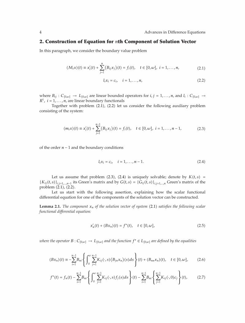
2. Construction of Equation for nth Component of Solution Vector
In this paragraph, we consider the boundary value problem
(Mix)(t) ≡ x′i(t) +
n∑
j=1
(Bijxj
)(t) = fi(t), t ∈ [0, ω], i = 1, . . . , n, (2.1)
lixi = ci, i = 1, . . . , n, (2.2)
where Bij : C[0,ω] → L[0,ω] are linear bounded operators for i, j = 1, . . . , n, and li : C[0,ω] →R1, i = 1, . . . , n, are linear boundary functionals
Together with problem (2.1), (2.2) let us consider the following auxiliary problemconsisting of the system:
(mix)(t) ≡ x′i(t) +
n−1∑
j=1
(Bijxj
)(t) = fi(t), t ∈ [0, ω], i = 1, . . . , n − 1, (2.3)
of the order n − 1 and the boundary conditions
lixi = ci, i = 1, . . . , n − 1. (2.4)
Let us assume that problem (2.3), (2.4) is uniquely solvable; denote by K(t, s) ={Kij(t, s)}i,j=1,...,n−1 its Green’s matrix and by G(t, s) = {Gij(t, s)}i,j=1,...,n Green’s matrix of theproblem (2.1), (2.2).
Let us start with the following assertion, explaining how the scalar functionaldifferential equation for one of the components of the solution vector can be constructed.
Lemma 2.1. The component xn of the solution vector of system (2.1) satisfies the following scalarfunctional differential equation:
x′n(t) + (Bxn)(t) = f∗(t), t ∈ [0, ω], (2.5)
where the operator B : C[0,ω] → L[0,ω] and the function f∗ ∈ L[0,ω] are defined by the equalities
(Bxn)(t) ≡ −n−1∑
i=1
Bni
⎧⎨
⎩
∫ω
0
n−1∑
j=1
Kij(·, s)(Bjnxn
)(s)ds
⎫⎬
⎭(t) + (Bnnxn)(t), t ∈ [0, ω], (2.6)
f∗(t) = fn(t) −n−1∑
i=1
Bni
⎧⎨
⎩
∫ω
0
n−1∑
j=1
Kij(·, s)fj(s)ds⎫⎬
⎭(t) −n−1∑
i=1
Bni
⎧⎨
⎩
n−1∑
j=1
Kij(·, 0)cj
⎫⎬
⎭(t), (2.7)
Advances in Difference Equations 5
where u = col{u1, . . . , un−1} is the solution of the system
(mix)(t) = 0, t ∈ [0, ω], i = 1, . . . , n − 1, (2.8)
satisfying condition (2.4).
Proof. Using Green’s matrix K(t, s) = {Kij(t, s)}n−1i,j=1 of problem (2.3), (2.4), we obtain
xi(t) = −∫ω
0
n−1∑
j=1
Kij(t, s)(Bjnxn
)(s)ds +
∫ω
0
n−1∑
j=1
Kij(t, s)fj(s)ds +n−1∑
j=1
Kij(t, 0)cj , (2.9)
for every i ∈ {1, . . . , n − 1}. Substitution of these representations in the nth equation of thesystem (2.1) leads to (2.5), where the operatorB and the function f∗ are described by formulas(2.6) and (2.7), respectively.
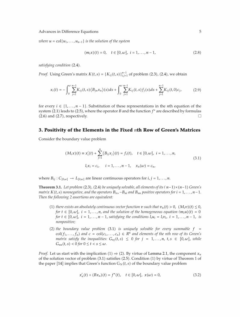
3. Positivity of the Elements in the Fixed nth Row of Green’s Matrices
Consider the boundary value problem
(Mix)(t) ≡ x′i(t) +
n∑
j=1
(Bijxj
)(t) = fi(t), t ∈ [0, ω], i = 1, . . . , n,
lixi = ci, i = 1, . . . , n − 1, xn(ω) = cn,
(3.1)
where Bij : C[0,ω] → L[0,ω] are linear continuous operators for i, j = 1, . . . , n.
Theorem 3.1. Let problem (2.3), (2.4) be uniquely solvable, all elements of its ( n−1)×(n−1)Green’smatrixK(t, s) nonnegative, and the operators Bin,−Bni and Bnn positive operators for i = 1, . . . , n−1.Then the following 2 assertions are equivalent:
(1) there exists an absolutely continuous vector function v such that vn(t) > 0, (Miv)(t) ≤ 0,for t ∈ [0, ω], i = 1, . . . , n, and the solution of the homogeneous equation (miu)(t) = 0for t ∈ [0, ω], i = 1, . . . , n − 1, satisfying the conditions liui = livi, i = 1, . . . , n − 1, isnonpositive;
(2) the boundary value problem (3.1) is uniquely solvable for every summable f =col(f1, . . . , fn) and c = col(c1, . . . , cn) ∈ Rn and elements of the nth row of its Green’smatrix satisfy the inequalities: Gnj(t, s) ≤ 0 for j = 1, . . . , n, t, s ∈ [0, ω], whileGnn(t, s) < 0 for 0 ≤ t < s ≤ ω.
Proof. Let us start with the implication (1) ⇒ (2). By virtue of Lemma 2.1, the component xn
of the solution vector of problem (3.1) satisfies (2.5). Condition (1) by virtue of Theorem 1 ofthe paper [14] implies that Green’s function GN(t, s) of the boundary value problem
x′n(t) + (Bxn)(t) = f∗(t), t ∈ [0, ω], x(ω) = 0, (3.2)
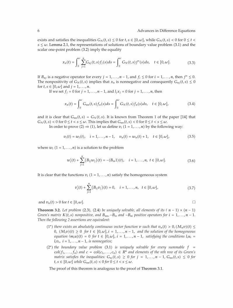
6 Advances in Difference Equations
exists and satisfies the inequalities GN(t, s) ≤ 0 for t, s ∈ [0, ω], while GN(t, s) < 0 for 0 ≤ t <s ≤ ω. Lemma 2.1, the representations of solutions of boundary value problem (3.1) and thescalar one-point problem (3.2) imply the equality
xn(t) =∫ω
0
n∑
j=1
Gnj(t, s)fj(s)ds =∫ω
0GN(t, s)f∗(s)ds, t ∈ [0, ω]. (3.3)
If Bnj is a negative operator for every j = 1, . . . , n − 1, and fi ≤ 0 for i = 1, . . . , n, then f∗ ≤ 0.The nonpositivity of GN(t, s) implies that xn is nonnegative and consequently Gnj(t, s) ≤ 0for t, s ∈ [0, ω] and j = 1, . . . , n.
If we set fj = 0 for j = 1, . . . , n − 1, and ljxj = 0 for j = 1, . . . , n, then
xn(t) =∫ω
0Gnn(t, s)fn(s)ds =
∫ω
0GN(t, s)fn(s)ds, t ∈ [0, ω], (3.4)
and it is clear that Gnn(t, s) = GN(t, s). It is known from Theorem 1 of the paper [14] thatGN(t, s) < 0 for 0 ≤ t < s ≤ ω. This implies that Gnn(t, s) < 0 for 0 ≤ t < s ≤ ω.
In order to prove (2) ⇒ (1), let us define vi (1 = 1, . . . , n) by the following way:
vi(t) = wi(t), i = 1, . . . , n − 1, vn(t) = wn(t) + 1, t ∈ [0, ω], (3.5)
where wi (1 = 1, . . . , n) is a solution to the problem
w′i(t) +
n∑
j=1
(Bijwj
)(t) = −(Bin1)(t), i = 1, . . . , n, t ∈ [0, ω]. (3.6)
It is clear that the functions vi (1 = 1, . . . , n) satisfy the homogeneous system
v′i(t) +
n∑
j=1
(Bijvj
)(t) = 0, i = 1, . . . , n, t ∈ [0, ω], (3.7)
and vn(t) > 0 for t ∈ [0, ω].
Theorem 3.2. Let problem (2.3), (2.4) be uniquely solvable, all elements of its ( n − 1) × (n − 1)Green’s matrix K(t, s) nonpositive, and Bnn,−Bin and −Bni positive operators for i = 1, . . . , n − 1.Then the following 2 assertions are equivalent:
(1∗) there exists an absolutely continuous vector function v such that vn(t) > 0, (Mnv)(t) ≤0, (Miv)(t) ≥ 0 for t ∈ [0, ω], i = 1, . . . , n − 1, and the solution of the homogeneousequation (miu)(t) = 0 for t ∈ [0, ω], i = 1, . . . , n − 1, satisfying the conditions liui =livi, i = 1, . . . , n − 1, is nonnegative;
(2∗) the boundary value problem (3.1) is uniquely solvable for every summable f =col(f1, . . . , fn) and c = col(c1, . . . , cn) ∈ Rn and elements of the nth row of its Green’smatrix satisfies the inequalities: Gnj(t, s) ≥ 0 for j = 1, . . . , n − 1, Gnn(t, s) ≤ 0 fort, s ∈ [0, ω] while Gnn(t, s) < 0 for 0 ≤ t < s ≤ ω.
The proof of this theorem is analogous to the proof of Theorem 3.1.

Advances in Difference Equations 7
4. Sufficient Conditions of Nonpositivity of the Elements inthe nth Row of Green’s Matrices for System of OrdinaryDifferential Equations
In this paragraph, we consider the system of the ordinary differential equations
x′i(t) +
n∑
j=1
pij(t)xj(t) = fi(t), i = 1, . . . , n, t ∈ [0, ω], (4.1)
with the boundary conditions
xi(0) = xi(ω) + ci, i = 1, . . . , n − 1, xn(ω) = cn. (4.2)
Theorem 4.1. Let the following conditions be fulfilled:
(1) pij ≤ 0 for i /= j, i, j = 1, . . . , n − 1;
(2) pjn ≥ 0, pnj ≤ 0 for j = 1, . . . , n − 1, pnn ≥ 0;
(3) there exists a positive number α such that
pnn(t) −n−1∑
j=1
pnj(t) ≤ α ≤ min1≤i≤n−1
⎧⎨
⎩−pin(t) +n−1∑
j=1
pij(t)
⎫⎬
⎭, t ∈ [0, ω]. (4.3)
Then problem (4.1), (4.2) is uniquely solvable for every summable f = col(f1, f2, fn) and c =col(c1, c2, . . . , cn) ∈ Rn, and the elements of the nth row of Green’s matrix of boundary value problem(4.1), (4.2) satisfy the inequalities: Gnj(t, s) ≤ 0 for j = 1, . . . , n, for t, s ∈ [0, ω], Gnn(t, s) < 0 for0 ≤ t < s ≤ ω.
Proof. Let us prove that all elements of Green’s matrixK(t, s) of the auxiliary boundary valueproblem
x′i(t) +
n−1∑
j=1
pij(t)xj(t) = fi(t), i = 1, . . . , n − 1, t ∈ [0, ω],
xi(0) = xi(ω) + ci, i = 1, . . . , n − 1,
(4.4)
are nonnegative. The conditions (1), (2), and the inequality
0 < α ≤ min1≤i≤n−1
⎧⎨
⎩−pin(t) +n−1∑
j=1
pij(t)
⎫⎬
⎭, t ∈ [0, ω], (4.5)
imply that the conditions (1) and (2) of Theorem 3.1 of the paper [13] are fulfilled. Assertion(a) of Theorem 3.1 [13] is fulfilled. To prove it, we set vi = 1 for 1 = 1, . . . , n−1 in this assertion.
8 Advances in Difference Equations
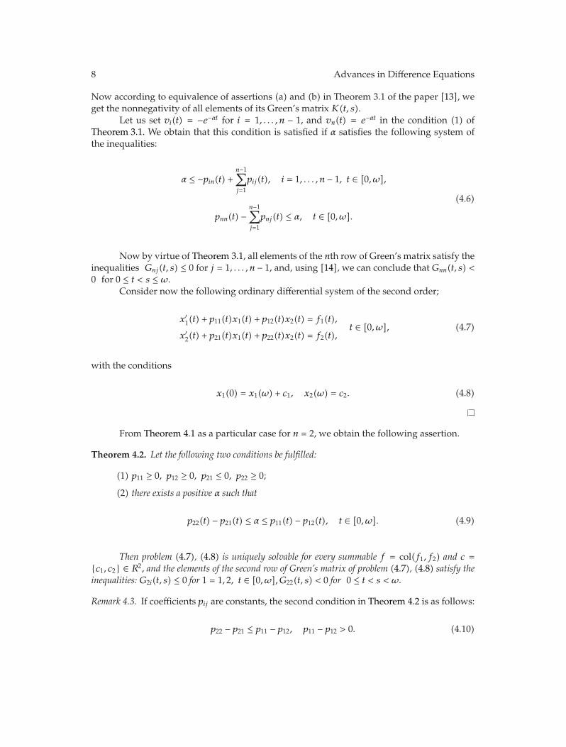
Now according to equivalence of assertions (a) and (b) in Theorem 3.1 of the paper [13], weget the nonnegativity of all elements of its Green’s matrix K(t, s).
Let us set vi(t) = −e−αt for i = 1, . . . , n − 1, and vn(t) = e−αt in the condition (1) ofTheorem 3.1. We obtain that this condition is satisfied if α satisfies the following system ofthe inequalities:
α ≤ −pin(t) +n−1∑
j=1
pij(t), i = 1, . . . , n − 1, t ∈ [0, ω],
pnn(t) −n−1∑
j=1
pnj(t) ≤ α, t ∈ [0, ω].
(4.6)
Now by virtue of Theorem 3.1, all elements of the nth row of Green’s matrix satisfy theinequalities Gnj(t, s) ≤ 0 for j = 1, . . . , n − 1, and, using [14], we can conclude that Gnn(t, s) <0 for 0 ≤ t < s ≤ ω.
Consider now the following ordinary differential system of the second order;
x′1(t) + p11(t)x1(t) + p12(t)x2(t) = f1(t),
x′2(t) + p21(t)x1(t) + p22(t)x2(t) = f2(t),
t ∈ [0, ω], (4.7)
with the conditions
x1(0) = x1(ω) + c1, x2(ω) = c2. (4.8)
From Theorem 4.1 as a particular case for n = 2, we obtain the following assertion.
Theorem 4.2. Let the following two conditions be fulfilled:
(1) p11 ≥ 0, p12 ≥ 0, p21 ≤ 0, p22 ≥ 0;
(2) there exists a positive α such that
p22(t) − p21(t) ≤ α ≤ p11(t) − p12(t), t ∈ [0, ω]. (4.9)
Then problem (4.7), (4.8) is uniquely solvable for every summable f = col(f1, f2) and c ={c1, c2} ∈ R2, and the elements of the second row of Green’s matrix of problem (4.7), (4.8) satisfy theinequalities: G2i(t, s) ≤ 0 for 1 = 1, 2, t ∈ [0, ω], G22(t, s) < 0 for 0 ≤ t < s < ω.
Remark 4.3. If coefficients pij are constants, the second condition in Theorem 4.2 is as follows:
p22 − p21 ≤ p11 − p12, p11 − p12 > 0. (4.10)
Advances in Difference Equations 9
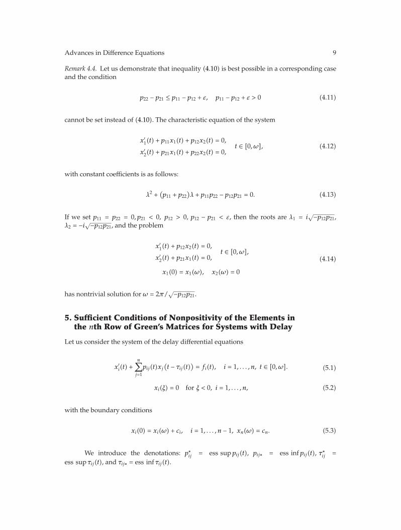
Remark 4.4. Let us demonstrate that inequality (4.10) is best possible in a corresponding caseand the condition
p22 − p21 ≤ p11 − p12 + ε, p11 − p12 + ε > 0 (4.11)
cannot be set instead of (4.10). The characteristic equation of the system
x′1(t) + p11x1(t) + p12x2(t) = 0,
x′2(t) + p21x1(t) + p22x2(t) = 0,
t ∈ [0, ω], (4.12)
with constant coefficients is as follows:
λ2 +(p11 + p22
)λ + p11p22 − p12p21 = 0. (4.13)
If we set p11 = p22 = 0, p21 < 0, p12 > 0, p12 − p21 < ε, then the roots are λ1 = i√−p12p21,
λ2 = −i√−p12p21, and the problem
x′1(t) + p12x2(t) = 0,
x′2(t) + p21x1(t) = 0,
t ∈ [0, ω],
x1(0) = x1(ω), x2(ω) = 0
(4.14)
has nontrivial solution for ω = 2π/√−p12p21.
5. Sufficient Conditions of Nonpositivity of the Elements inthe nth Row of Green’s Matrices for Systems with Delay
Let us consider the system of the delay differential equations
x′i(t) +
n∑
j=1
pij(t)xj
(t − τij(t)
)= fi(t), i = 1, . . . , n, t ∈ [0, ω]. (5.1)
xi(ξ) = 0 for ξ < 0, i = 1, . . . , n, (5.2)
with the boundary conditions
xi(0) = xi(ω) + ci, i = 1, . . . , n − 1, xn(ω) = cn. (5.3)
We introduce the denotations: p∗ij = ess sup pij(t), pij∗ = ess inf pij(t), τ∗ij =ess sup τij(t), and τij∗ = ess inf τij(t).
10 Advances in Difference Equations
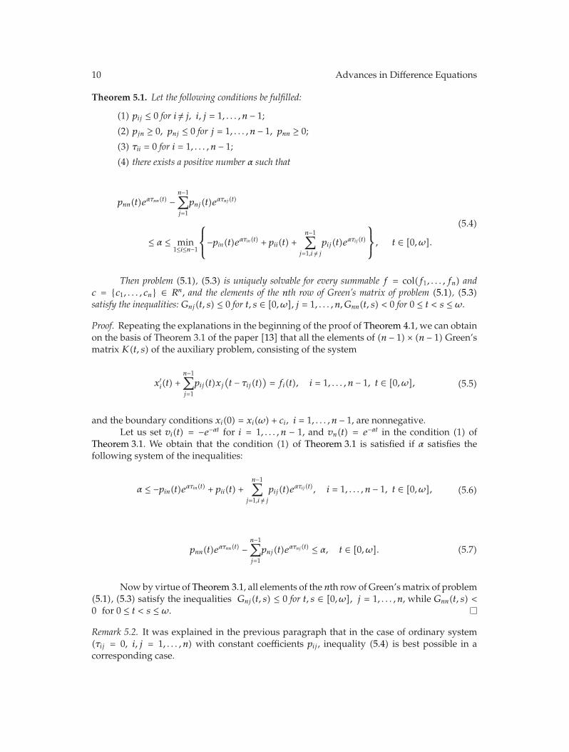
Theorem 5.1. Let the following conditions be fulfilled:
(1) pij ≤ 0 for i /= j, i, j = 1, . . . , n − 1;
(2) pjn ≥ 0, pnj ≤ 0 for j = 1, . . . , n − 1, pnn ≥ 0;
(3) τii = 0 for i = 1, . . . , n − 1;
(4) there exists a positive number α such that
pnn(t)eατnn(t) −n−1∑
j=1
pnj(t)eατnj (t)
≤ α ≤ min1≤i≤n−1
⎧⎨
⎩−pin(t)eατin(t) + pii(t) +n−1∑
j=1,i /= j
pij(t)eατij (t)
⎫⎬
⎭, t ∈ [0, ω].
(5.4)
Then problem (5.1), (5.3) is uniquely solvable for every summable f = col(f1, . . . , fn) andc = {c1, . . . , cn} ∈ Rn, and the elements of the nth row of Green’s matrix of problem (5.1), (5.3)satisfy the inequalities: Gnj(t, s) ≤ 0 for t, s ∈ [0, ω], j = 1, . . . , n, Gnn(t, s) < 0 for 0 ≤ t < s ≤ ω.
Proof. Repeating the explanations in the beginning of the proof of Theorem 4.1, we can obtainon the basis of Theorem 3.1 of the paper [13] that all the elements of (n − 1) × (n − 1) Green’smatrix K(t, s) of the auxiliary problem, consisting of the system
x′i(t) +
n−1∑
j=1
pij(t)xj
(t − τij(t)
)= fi(t), i = 1, . . . , n − 1, t ∈ [0, ω], (5.5)
and the boundary conditions xi(0) = xi(ω) + ci, i = 1, . . . , n − 1, are nonnegative.Let us set vi(t) = −e−αt for i = 1, . . . , n − 1, and vn(t) = e−αt in the condition (1) of
Theorem 3.1. We obtain that the condition (1) of Theorem 3.1 is satisfied if α satisfies thefollowing system of the inequalities:
α ≤ −pin(t)eατin(t) + pii(t) +n−1∑
j=1,i /= j
pij(t)eατij (t), i = 1, . . . , n − 1, t ∈ [0, ω], (5.6)
pnn(t)eατnn(t) −n−1∑
j=1
pnj(t)eατnj (t) ≤ α, t ∈ [0, ω]. (5.7)
Nowby virtue of Theorem 3.1, all elements of the nth row of Green’smatrix of problem(5.1), (5.3) satisfy the inequalities Gnj(t, s) ≤ 0 for t, s ∈ [0, ω], j = 1, . . . , n, while Gnn(t, s) <0 for 0 ≤ t < s ≤ ω.
Remark 5.2. It was explained in the previous paragraph that in the case of ordinary system(τij = 0, i, j = 1, . . . , n) with constant coefficients pij , inequality (5.4) is best possible in acorresponding case.
Advances in Difference Equations 11
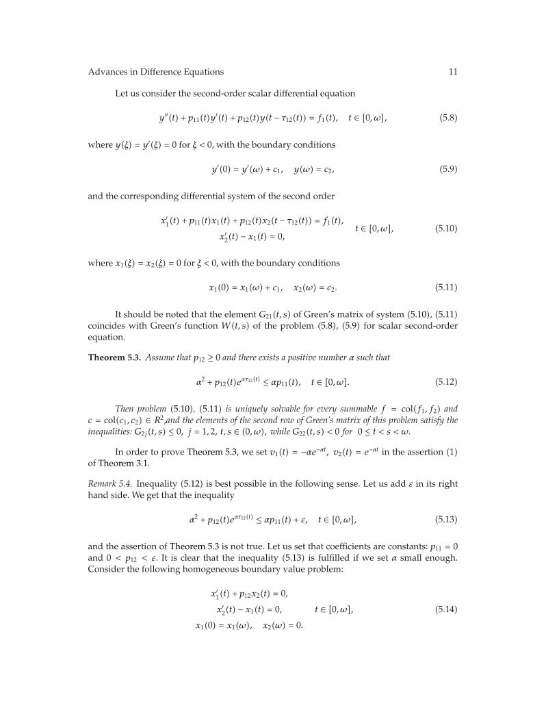
Let us consider the second-order scalar differential equation
y′′(t) + p11(t)y′(t) + p12(t)y(t − τ12(t)) = f1(t), t ∈ [0, ω], (5.8)
where y(ξ) = y′(ξ) = 0 for ξ < 0, with the boundary conditions
y′(0) = y′(ω) + c1, y(ω) = c2, (5.9)
and the corresponding differential system of the second order
x′1(t) + p11(t)x1(t) + p12(t)x2(t − τ12(t)) = f1(t),
x′2(t) − x1(t) = 0,
t ∈ [0, ω], (5.10)
where x1(ξ) = x2(ξ) = 0 for ξ < 0, with the boundary conditions
x1(0) = x1(ω) + c1, x2(ω) = c2. (5.11)
It should be noted that the element G21(t, s) of Green’s matrix of system (5.10), (5.11)coincides with Green’s function W(t, s) of the problem (5.8), (5.9) for scalar second-orderequation.
Theorem 5.3. Assume that p12 ≥ 0 and there exists a positive number α such that
α2 + p12(t)eατ12(t) ≤ αp11(t), t ∈ [0, ω]. (5.12)
Then problem (5.10), (5.11) is uniquely solvable for every summable f = col(f1, f2) andc = col(c1, c2) ∈ R2,and the elements of the second row of Green’s matrix of this problem satisfy theinequalities: G2j(t, s) ≤ 0, j = 1, 2, t, s ∈ (0, ω), while G22(t, s) < 0 for 0 ≤ t < s < ω.
In order to prove Theorem 5.3, we set v1(t) = −αe−αt, v2(t) = e−αt in the assertion (1)of Theorem 3.1.
Remark 5.4. Inequality (5.12) is best possible in the following sense. Let us add ε in its righthand side. We get that the inequality
α2 + p12(t)eατ12(t) ≤ αp11(t) + ε, t ∈ [0, ω], (5.13)
and the assertion of Theorem 5.3 is not true. Let us set that coefficients are constants: p11 = 0and 0 < p12 < ε. It is clear that the inequality (5.13) is fulfilled if we set α small enough.Consider the following homogeneous boundary value problem:
x′1(t) + p12x2(t) = 0,
x′2(t) − x1(t) = 0,
x1(0) = x1(ω), x2(ω) = 0.
t ∈ [0, ω], (5.14)

12 Advances in Difference Equations
The components x1, x2 of the solution vector are periodic and for ω = 2π/√p12 the boundaryvalue problem (5.14) has a nontrivial solution.
Let us prove the following assertions, giving an efficient test of nonpositivity of theelements in the nth row of Green’s matrix in the case when the coefficients |pnj | are smallenough for j = 1, . . . , n − 1.
Theorem 5.5. Let the following conditions be fulfilled:
(1) pij ≤ 0 for i /= j, i, j = 1, . . . , n − 1;
(2) pjn ≥ 0, pnj ≤ 0, pnn ≥ 0 for j = 1, . . . , n − 1;
(3) τnn = const > 0, and other delays τij are zeros;
(4) the inequalities
pnn(t)τnn exp
⎧⎨
⎩τnnn−1∑
j=1
∣∣pnj∣∣∗⎫⎬
⎭ ≤ 1e, t ∈ [0, ω], (5.15)
1τnn
+n−1∑
j=1
∣∣pnj∣∣∗ ≤ min
1≤i≤n−1
⎧⎨
⎩−pin(t) +n∑
j=1,i /= j
pij(t)
⎫⎬
⎭, t ∈ [0, ω], (5.16)
are fulfilled.Then problem (5.1), (5.3) is uniquely solvable for every summable f = col(f1, f2, . . . , fn) and
c = (c1, c2, . . . , cn) ∈ Rn, and the elements of the nth row of its Green’s matrix satisfy the inequalities:Gnj(t, s) ≤ 0 for j = 1, . . . , n, while Gnn(t, s) < 0 for 0 < t < s < ω.
Proof. Let us set vi(t) = −e−αt for i = 1, . . . , n − 1, and vn(t) = e−αt in the condition (1) ofTheorem 3.1.
pnn(t)eατnn −n−1∑
j=1
pnj(t) ≤ α ≤ min1≤i≤n−1
⎧⎨
⎩−pin(t) +n∑
j=1,i /= j
pij(t)
⎫⎬
⎭, t ∈ [0, ω]. (5.17)
In the left-hand side, we have the inequality
pnn(t)eατnn −n−1∑
j=1
pnj(t) ≤ α, t ∈ [0, ω], (5.18)
which is fulfilled when
pnn(t) ≤⎧⎨
⎩α −n−1∑
j=1
∣∣pnj∣∣∗⎫⎬
⎭e−ατnn , [0, ω]. (5.19)
The right-hand side in inequality (5.18) gets its maximum for α = 1/τnn +∑n−1
j=1 |pnj |∗.Substituting this α into (5.19) and the right part of (5.17), we obtain inequalities (5.15) and(5.16).
Advances in Difference Equations 13
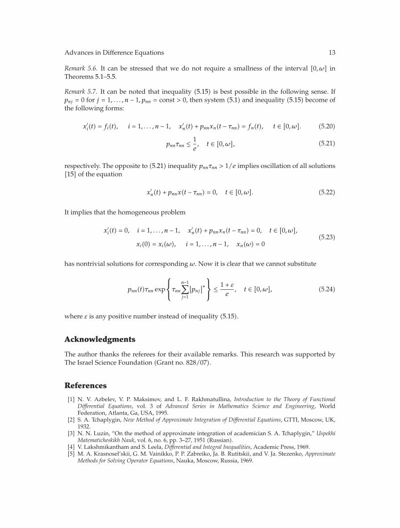
Remark 5.6. It can be stressed that we do not require a smallness of the interval [0, ω] inTheorems 5.1–5.5.
Remark 5.7. It can be noted that inequality (5.15) is best possible in the following sense. Ifpnj = 0 for j = 1, . . . , n − 1, pnn = const > 0, then system (5.1) and inequality (5.15) become ofthe following forms:
x′i(t) = fi(t), i = 1, . . . , n − 1, x′
n(t) + pnnxn(t − τnn) = fn(t), t ∈ [0, ω]. (5.20)
pnnτnn ≤ 1e, t ∈ [0, ω], (5.21)
respectively. The opposite to (5.21) inequality pnnτnn > 1/e implies oscillation of all solutions[15] of the equation
x′n(t) + pnnx(t − τnn) = 0, t ∈ [0, ω]. (5.22)
It implies that the homogeneous problem
x′i(t) = 0, i = 1, . . . , n − 1, x′
n(t) + pnnxn(t − τnn) = 0, t ∈ [0, ω],
xi(0) = xi(ω), i = 1, . . . , n − 1, xn(ω) = 0(5.23)
has nontrivial solutions for corresponding ω. Now it is clear that we cannot substitute
pnn(t)τnn exp
⎧⎨
⎩τnnn−1∑
j=1
∣∣pnj∣∣∗⎫⎬
⎭ ≤ 1 + ε
e, t ∈ [0, ω], (5.24)
where ε is any positive number instead of inequality (5.15).
Acknowledgments
The author thanks the referees for their available remarks. This research was supported byThe Israel Science Foundation (Grant no. 828/07).
References
[1] N. V. Azbelev, V. P. Maksimov, and L. F. Rakhmatullina, Introduction to the Theory of FunctionalDifferential Equations, vol. 3 of Advanced Series in Mathematics Science and Engineering, WorldFederation, Atlanta, Ga, USA, 1995.
[2] S. A. Tchaplygin, New Method of Approximate Integration of Differential Equations, GTTI, Moscow, UK,1932.
[3] N. N. Luzin, “On the method of approximate integration of academician S. A. Tchaplygin,” UspekhiMatematicheskikh Nauk, vol. 6, no. 6, pp. 3–27, 1951 (Russian).
[4] V. Lakshmikantham and S. Leela, Differential and Integral Inequalities, Academic Press, 1969.[5] M. A. Krasnosel’skii, G. M. Vainikko, P. P. Zabreiko, Ja. B. Rutitskii, and V. Ja. Stezenko, Approximate
Methods for Solving Operator Equations, Nauka, Moscow, Russia, 1969.
14 Advances in Difference Equations
[6] I. Kiguradze and B. Puza, “On boundary value problems for systems of linear functional-differentialequations,” Czechoslovak Mathematical Journal, vol. 47, no. 2, pp. 341–373, 1997.
[7] I. Kiguradze and B. Puza, Boundary Value Problems for Systems of Linear Functional Differential Equations,vol. 12 of Folia Facultatis Scientiarium Naturalium Universitatis Masarykianae Brunensis. Mathematica,FOLIA, Masaryk University, Brno, Czech Republic, 2003.
[8] I. T. Kiguradze, “Boundary value problems for systems of ordinary differential equations,” in CurrentProblems in Mathematics. Newest Results, vol. 30 of Itogi Nauki i Tekhniki, pp. 3–103, Akad. Nauk SSSRVsesoyuz. Inst. Nauchn. i Tekhn. Inform., Moscow, Russia, 1987, English translated in Journal of SovietMathematics, vol. 43, no. 2, 2259–2339, 1988.
[9] T. Wazewski, “Systemes des equations et des inegalites differentielles ordinaires aux deuxiemesmembres monotones et leurs applications,” Annales Polonici Mathematici, vol. 23, pp. 112–166, 1950.
[10] R. P. Agarwal and A. Domoshnitsky, “Non-oscillation of the first-order differential equations withunbounded memory for stabilization by control signal,” Applied Mathematics and Computation, vol.173, no. 1, pp. 177–195, 2006.
[11] A. Domoshnitsky, “Maximum principles and nonoscillation intervals for first order Volterrafunctional differential equations,” Dynamics of Continuous, Discrete & Impulsive Systems A, vol. 15,no. 6, pp. 769–814, 2008.
[12] R. Hakl, A. Lomtatidze, and J. Sremr, Some Boundary Value Problems for First Order Scalar FunctionalDifferential Equations, FOLIA, Masaryk University, Brno, Czech Republic, 2002.
[13] R. P. Agarwal and A. Domoshnitsky, “On positivity of several components of solution vector forsystems of linear functional differential equations,” Glasgow Mathematical Journal, vol. 52, no. 1, pp.115–136, 2010.
[14] A. Domoshnitsky, “New concept in the study of differential inequalities,” in Functional-DifferentialEquations, vol. 1 of Functional Differential Equations, Israel Seminar, pp. 52–59, The College of Judea &Samaria, Ariel, Israel, 1993.
[15] I. Gyori and G. Ladas, Oscillation Theory of Delay Differential Equations, Oxford MathematicalMonographs, The Clarendon Press, Oxford University Press, New York, NY, USA, 1991.