Differential equations - Physicsntg/6810/readings/hjorth-jensen_notes... · Differential equations If God has made the world a perfect mechanism, ... We are interested in solving

Chapter 8

Differential equations

If God has made the world a perfect mechanism, he has at least conceded so much to our imperfectintellect that in order to predict little parts of it, we need not solve innumerable differential equations,but can use dice with fair success. Max Born, quoted in H. R. Pagels, The Cosmic Code [40]

Abstract This chapter aims at giving an overview on some of the most used methods tosolve ordinary differential equations. Several examples of applications to physical systemsare discussed, from the classical pendulum to the physics of Neutron stars.

8.1 Introduction

We may trace the origin of differential equations back to Newton in 16871 and his treatise onthe gravitational force and what is known to us as Newton’s second law in dynamics.

Needless to say, differential equations pervade the sciences and are to us the tools by whichwe attempt to express in a concise mathematical language the laws of motion of nature. Weuncover these laws via the dialectics between theories, simulations and experiments, and weuse them on a daily basis which spans from applications in engineering or financial engineer-ing to basic research in for example biology, chemistry, mechanics, physics, ecological modelsor medicine.

We have already met the differential equation for radioactive decay in nuclear physics.Other famous differential equations are Newton’s law of cooling in thermodynamics. thewave equation, Maxwell’s equations in electromagnetism, the heat equation in thermody-namic, Laplace’s equation and Poisson’s equation, Einstein’s field equation in general relativ-ity, Schrödinger equation in quantum mechanics, the Navier-Stokes equations in fluid dynam-ics, the Lotka-Volterra equation in population dynamics, the Cauchy-Riemann equations incomplex analysis and the Black-Scholes equation in finance, just to mention a few. Excellenttexts on differential equations and computations are the texts of Eriksson, Estep, Hansbo andJohnson [41], Butcher [42] and Hairer, Nørsett and Wanner [43].

There are five main types of differential equations,

• ordinary differential equations (ODEs), discussed in this chapter for initial value problemsonly. They contain functions of one independent variable, and derivatives in that variable.The next chapter deals with ODEs and boundary value problems.

• Partial differential equations with functions of multiple independent variables and theirpartial derivatives, covered in chapter 10.

1 Newton had most of the relations for his laws ready 22 years earlier, when according to legend he wascontemplating falling apples. However, it took more than two decades before he published his theories, chieflybecause he was lacking an essential mathematical tool, differential calculus.

243

244 8 Differential equations

• So-called delay differential equations that involve functions of one dependent variable,derivatives in that variable, and depend on previous states of the dependent variables.

• Stochastic differential equations (SDEs) are differential equations in which one or more ofthe terms is a stochastic process, thus resulting in a solution which is itself a stochasticprocess.

• Finally we have so-called differential algebraic equations (DAEs). These are differentialequation comprising differential and algebraic terms, given in implicit form.

In this chapter we restrict the attention to ordinary differential equations. We focus oninitial value problems and present some of the more commonly used methods for solving suchproblems numerically. The physical systems which are discussed range from the classicalpendulum with non-linear terms to the physics of a neutron star or a white dwarf.

8.2 Ordinary differential equations

In this section we will mainly deal with ordinary differential equations and numerical methodssuitable for dealing with them. However, before we proceed, a brief remainder on differentialequations may be appropriate.

• The order of the ODE refers to the order of the derivative on the left-hand side in theequation

dydt

= f (t,y).

This equation is of first order and f is an arbitrary function. A second-order equation goestypically like

d2ydt2

= f (t,dydt

,y).

A well-known second-order equation is Newton’s second law

md2xdt2

=!kx, (8.1)

where k is the force constant. ODE depend only on one variable, whereas• partial differential equations like the time-dependent Schrödinger equation

i h∂ψ(x, t)

∂ t=

h2

2m

!∂ 2ψ(r, t)∂x2 +

∂ 2ψ(r, t)∂y2 +

∂ 2ψ(r, t)∂ z2

"+V(x)ψ(x, t),

may depend on several variables. In certain cases, like the above equation, the wave func-tion can be factorized in functions of the separate variables, so that the Schrödinger equa-tion can be rewritten in terms of sets of ordinary differential equations.

• We distinguish also between linear and non-linear differential equation where e.g.,

dydt

= g3(t)y(t),

is an example of a linear equation, while

dydt

= g3(t)y(t)! g(t)y2(t),

is a non-linear ODE. Another concept which dictates the numerical method chosen forsolving an ODE, is that of initial and boundary conditions. To give an example, in our study

8.3 Finite difference methods 245

of neutron stars below, we will need to solve two coupled first-order differential equations,one for the total mass m and one for the pressure P as functions of ρ

dmdr

= 4πr2ρ(r)/c2,

anddPdr

=!Gm(r)r2 ρ(r)/c2.

where ρ is the mass-energy density. The initial conditions are dictated by the mass beingzero at the center of the star, i.e., when r = 0, yielding m(r = 0) = 0. The other condition isthat the pressure vanishes at the surface of the star. This means that at the point wherewe have P = 0 in the solution of the integral equations, we have the total radius R of thestar and the total mass m(r= R). These two conditions dictate the solution of the equations.Since the differential equations are solved by stepping the radius from r = 0 to r = R, so-called one-step methods (see the next section) or Runge-Kutta methods may yield stablesolutions.In the solution of the Schrödinger equation for a particle in a potential, we may need toapply boundary conditions as well, such as demanding continuity of the wave function andits derivative.

• In many cases it is possible to rewrite a second-order differential equation in terms of twofirst-order differential equations. Consider again the case of Newton’s second law in Eq.(8.1). If we define the position x(t) = y(1)(t) and the velocity v(t) = y(2)(t) as its derivative

dy(1)(t)dt

=dx(t)dt

= y(2)(t),

we can rewrite Newton’s second law as two coupled first-order differential equations

mdy(2)(t)dt

=!kx(t) =!ky(1)(t), (8.2)

anddy(1)(t)dt

= y(2)(t). (8.3)

8.3 Finite difference methods

These methods fall under the general class of one-step methods. The algoritm is rather sim-ple. Suppose we have an initial value for the function y(t) given by

y0 = y(t = t0).

We are interested in solving a differential equation in a region in space [a,b]. We define a steph by splitting the interval in N sub intervals, so that we have

h=b! aN

.

With this step and the derivative of y we can construct the next value of the function y at

y1 = y(t1 = t0 + h),


and so forth. If the function is rather well-behaved in the domain [a,b], we can use a fixed stepsize. If not, adaptive steps may be needed. Here we concentrate on fixed-step methods only.Let us try to generalize the above procedure by writing the step yi+1 in terms of the previousstep yi

yi+1 = y(t = ti+ h) = y(ti)+ hΔ(ti,yi(ti))+O(hp+1),

where O(hp+1) represents the truncation error. To determine Δ , we Taylor expand our functiony

yi+1 = y(t = ti+ h) = y(ti)+ h!y"(ti)+ · · ·+ y(p)(ti)

hp!1

p!

"+O(hp+1), (8.4)

where we will associate the derivatives in the parenthesis with

Δ(ti,yi(ti)) = (y"(ti)+ · · ·+ y(p)(ti)hp!1

p!). (8.5)

We definey"(ti) = f (ti,yi)

and if we truncate Δ at the first derivative, we have

yi+1 = y(ti)+ h f (ti,yi)+O(h2), (8.6)

which when complemented with ti+1 = ti+ h forms the algorithm for the well-known Eulermethod. Note that at every step we make an approximation error of the order of O(h2), how-ever the total error is the sum over all steps N = (b! a)/h, yielding thus a global error whichgoes like NO(h2) # O(h). To make Euler’s method more precise we can obviously decrease h(increase N). However, if we are computing the derivative f numerically by e.g., the two-stepsformula

f "2c(x) =f (x+ h)! f (x)

h+O(h),

we can enter into roundoff error problems when we subtract two almost equal numbers f (x+h)! f (x) # 0. Euler’s method is not recommended for precision calculation, although it ishandy to use in order to get a first view how a solution may look like. As an example, considerNewton’s equation rewritten in Eqs. (8.2) and (8.3). We define y0 = y(1)(t = 0) an v0 = y(2)(t = 0).The first steps in Newton’s equations are then

y(1)1 = y0 + hv0 +O(h2)

andy(2)1 = v0! hy0k/m+O(h2).

The Euler method is asymmetric in time, since it uses information about the derivative at

the beginning of the time interval. This means that we evaluate the position at y(1)1 using the

velocity at y(2)0 = v0. A simple variation is to determine y(1)n+1 using the velocity at y(2)n+1, that is(in a slightly more generalized form)

y(1)n+1 = y(1)n + hy(2)n+1+O(h2)

andy(2)n+1 = y(2)n + han+O(h2).

The acceleration an is a function of an(y(1)n ,y(2)n , t) and needs to be evaluated as well. This is the

Euler-Cromer method.Let us then include the second derivative in our Taylor expansion. We have then


Δ(ti,yi(ti)) = f (ti)+h2d f (ti,yi)

dt+O(h3).

The second derivative can be rewritten as

y"" = f " =d fdt

=∂ f∂ t

+∂ f∂y

∂y∂ t

=∂ f∂ t

+∂ f∂y

f

and we can rewrite Eq. (8.4) as

yi+1 = y(t = ti+ h) = y(ti)+ h f (ti)+h2

2

!∂ f∂ t

+∂ f∂y

f"+O(h3),

which has a local approximation error O(h3) and a global error O(h2). These approximationscan be generalized by using the derivative f to arbitrary order so that we have

yi+1 = y(t = ti+ h) = y(ti)+ h( f (ti,yi)+ . . . f (p!1)(ti,yi)hp!1

p! )+O(hp+1).

These methods, based on higher-order derivatives, are in general not used in numerical com-putation, since they rely on evaluating derivatives several times. Unless one has analyticalexpressions for these, the risk of roundoff errors is large.

8.3.1 Improvements of Euler’s algorithm, higher-order methods

The most obvious improvements to Euler’s and Euler-Cromer’s algorithms, avoiding in addi-tion the need for computing a second derivative, is the so-called midpoint method. We havethen

y(1)n+1 = y(1)n +h2

#y(2)n+1 + y(2)n

$+O(h2)

andy(2)n+1 = y(2)n + han+O(h2),

yielding

y(1)n+1 = y(1)n + hy(2)n +h2

2an+O(h3)

implying that the local truncation error in the position is now O(h3), whereas Euler’s or Euler-Cromer’s methods have a local error of O(h2). Thus, the midpoint method yields a global errorwith second-order accuracy for the position and first-order accuracy for the velocity. However,although these methods yield exact results for constant accelerations, the error increases ingeneral with each time step.

One method that avoids this is the so-called half-step method. Here we define

y(2)n+1/2 = y(2)n!1/2 + han+O(h2),

andy(1)n+1 = y(1)n + hy(2)n+1/2+O(h2).

Note that this method needs the calculation of y(2)1/2. This is done using for example Euler’smethod

y(2)1/2 = y(2)0 +h2a0 +O(h2).


As this method is numerically stable, it is often used instead of Euler’s method. Anothermethod which one may encounter is the Euler-Richardson method with

y(2)n+1 = y(2)n + han+1/2+O(h2), (8.7)

andy(1)n+1 = y(1)n + hy(2)n+1/2+O(h2). (8.8)

8.3.2 Verlet and Leapfrog algorithms

Another set of popular algorithms, which are both numerically stable and easy to implementare the Verlet and Leapfrog algorithms. These algorithms are much used in so-called Molec-ular Dynamics applications, see for example Refs. [44, 45]. Consider again a second-orderdifferential equation like Newton’s second law, whose one-dimensional version reads

md2xdt2

= F(x, t),

which we rewrite in terms of two coupled differential equations

dxdt

= v(x, t) and dvdt

= F(x, t)/m= a(x, t).

If we now perform a Taylor expansion

x(t+ h) = x(t)+ hx(1)(t)+h2

2x(2)(t)+O(h3).

In our case the second derivative is know via Newton’s second law, namely x(2)(t) = a(x, t).If we add to the above equation the corresponding Taylor expansion for x(t! h), we obtain,using the discretized expressions

x(ti± h) = xi±1 and xi = x(ti),

xi+1 = 2xi! xi!1 + h2x(2)i +O(h4).

We note that the truncation error goes like O(h4) since all the odd terms cancel when weadd the two Taylor expansions. We see also that the velocity is not directly included in theequation since the function x(2) = a(x, t) is supposed to be known. If we need the velocityhowever, we can compute it using the well-known formula

x(1)i =xi+1! xi!1

2h+O(h2).

We note that the velocity has a truncation error which goes like O(h2). In for example so-calledMolecular dynamics calculations, since the acceleration is normally known via Newton’s sec-ond law, there is seldomly a need for computing the velocity. The above sets of equations forthe position x(t) and the velocity defines the Verlet formula. The Leapfrog algorithm is alsoeasily derived.

We can rewrite the above Taylor expansion for x(t+ h) as

x(t+ h) = x(t)+ h!x(1)(t)+

h2x(2)(t)

"+O(h3).


Noting that

x(1)(t+ h/2) =!x(1)(t)+

h2x(2)(t)

"+O(h2),

we obtainx(t+ h) = x(t)+ h+ x(1)(t+ h/2)+O(h3),

which needs to be combined with

x(1)(t+ h/2) = x(1)(t! h/2)+ hx(2)(t)+O(h2).

Again, there is a lower truncation error in h for the velocity. Furthermore, the positions andthe velocities are evaluated at different time steps. If one needs x(1)(t), this can be computedusing

x(1)(t) =!x(1)(t$ h/2)± h

2x(2)(t)

"+O(h2).

The initial conditions can be handled in similar ways and the inaccuracy which arises betweenx(1)(0) and x(1)(h/2) is normally ignored. Summarizing, the popular Leapfrog algorithm impliesthe evaluation of position and velocity at different time steps. The final algorithm is given bythe following steps

x(1)(t+ h/2) = x(1)(t! h/2)+ hx(2)(t)+O(h2),

which is used inx(t+ h) = x(t)+ h+ x(1)(t+ h/2)+O(h3),

and finally

x(1)(t+ h) = x(1)(t+ h/2)+h2x

(2)(t+ h)+O(h2),

8.3.3 Predictor-Corrector methods

Consider again the first-order differential equation

dydt

= f (t,y),

which solved with Euler’s algorithm results in the following algorithm

yi+1 # y(ti)+ h f (ti,yi)

with ti+1 = ti+h. This means geometrically that we compute the slope at yi and use it to predictyi+1 at a later time ti+1. We introduce k1 = f (ti,yi) and rewrite our prediction for yi+1 as

yi+1 # y(ti)+ hk1.

We can then use the prediction yi+1 to compute a new slope at ti+1 by defining k2 = f (ti+1,yi+1).We define the new value of yi+1 by taking the average of the two slopes, resulting in

yi+1 # y(ti)+h2(k1 + k2).

The algorithm is very simple,namely


1. Compute the slope at ti, that is define the quantity k1 = f (ti,yi).2. Make a predicition for the solution by computing yi+1 # y(ti)+ hk1 by Euler’s method.3. Use the predicition yi+1 to compute a new slope at ti+1 defining the quantity k2 =

f (ti+1,yi+1).4. Correct the value of yi+1 by taking the average of the two slopes yielding yi+1 # y(ti)+

h2(k1 + k2).

It can be shown [24] that this procedure results in a mathematical truncation which goeslike O(h2), to be contrasted with Euler’s method which runs as O(h). One additional functionevaluation yields a better error estimate.

This simple algorithm conveys the philosophy of a large class of methods called predictor-corrector methods, see chapter 15 of Ref. [36] for additional algorithms. A simple extensionis obviously to use Simpson’s method to approximate the integral

yi+1 = yi+% ti+1

tif (t,y)dt,

when we solve the differential equation by successive integrations. The next section dealswith a particular class of efficient methods for solving ordinary differential equations, namelyvarious Runge-Kutta methods.

8.4 More on finite difference methods, Runge-Kutta methods

Runge-Kutta (RK) methods are based on Taylor expansion formulae, but yield in general bet-ter algorithms for solutions of an ODE. The basic philosophy is that it provides an intermedi-ate step in the computation of yi+1.

To see this, consider first the following definitions

dydt

= f (t,y),

andy(t) =

%f (t,y)dt,

and

yi+1 = yi+% ti+1

tif (t,y)dt.

To demonstrate the philosophy behind RK methods, let us consider the second-order RKmethod, RK2. The first approximation consists in Taylor expanding f (t,y) around the cen-ter of the integration interval ti to ti+1, i.e., at ti+ h/2, h being the step. Using the midpointformula for an integral, defining y(ti+ h/2) = yi+1/2 and ti+ h/2 = ti+1/2, we obtain

% ti+1

tif (t,y)dt # h f (ti+1/2,yi+1/2)+O(h3).

This means in turn that we have

yi+1 = yi+ h f (ti+1/2,yi+1/2)+O(h3).

8.4 More on finite difference methods, Runge-Kutta methods 251

However, we do not know the value of yi+1/2. Here comes thus the next approximation, namely,we use Euler’s method to approximate yi+1/2. We have then

y(i+1/2) = yi+h2dydt

= y(ti)+h2f (ti,yi).

This means that we can define the following algorithm for the second-order Runge-Kuttamethod, RK2.

k1 = h f (ti,yi),

k2 = h f (ti+1/2,yi+ k1/2),

with the final valueyi+1 # yi+ k2 +O(h3).

The difference between the previous one-step methods is that we now need an intermedi-ate step in our evaluation, namely ti+ h/2 = t(i+1/2) where we evaluate the derivative f . Thisinvolves more operations, but the gain is a better stability in the solution. The fourth-orderRunge-Kutta, RK4, which we will employ in the solution of various differential equations be-low, is easily derived. The steps are as follows. We start again with the equation

yi+1 = yi+% ti+1

tif (t,y)dt,

but instead of approximating the integral with the midpoint rule, we use now Simpson’s ruleat ti+h/2, h being the step. Using Simpson’s formula for an integral, defining y(ti+h/2)= yi+1/2and ti+ h/2 = ti+1/2, we obtain

% ti+1

tif (t,y)dt #

h6&f (ti,yi)+ 4 f (ti+1/2,yi+1/2)+ f (ti+1,yi+1)

'+O(h5).

This means in turn that we have

yi+1 = yi+h6&f (ti,yi)+ 4 f (ti+1/2,yi+1/2)+ f (ti+1,yi+1)

'+O(h5).

However, we do not know the values of yi+1/2 and yi+1. The fourth-order Runge-Kutta methodsplits the midpoint evaluations in two steps, that is we have

yi+1 # yi+h6&f (ti,yi)+ 2 f (ti+1/2,yi+1/2)+ 2 f (ti+1/2,yi+1/2)+ f (ti+1,yi+1)

',

since we want to approximate the slope at yi+1/2 in two steps. The first two function evalua-tions are as for the second order Runge-Kutta method. The algorithm is as follows

1. We compute firstk1 = h f (ti,yi), (8.9)

which is nothing but the slope at ti.If we stop here we have Euler’s method.2. Then we compute the slope at the midpoint using Euler’s method to predict yi+1/2, as

in the second-order Runge-Kutta method. This leads to the computation of

k2 = h f (ti+ h/2,yi+ k1/2). (8.10)

3. The improved slope at the midpoint is used to further improve the slope of yi+1/2 bycomputing


k3 = h f (ti+ h/2,yi+ k2/2). (8.11)

4. With the latter slope we can in turn predict the value of yi+1 via the computation of

k4 = h f (ti+ h,yi+ k3). (8.12)

5. The final algorithm becomes then

yi+1 = yi+16(k1 + 2k2+ 2k3 + k4) . (8.13)

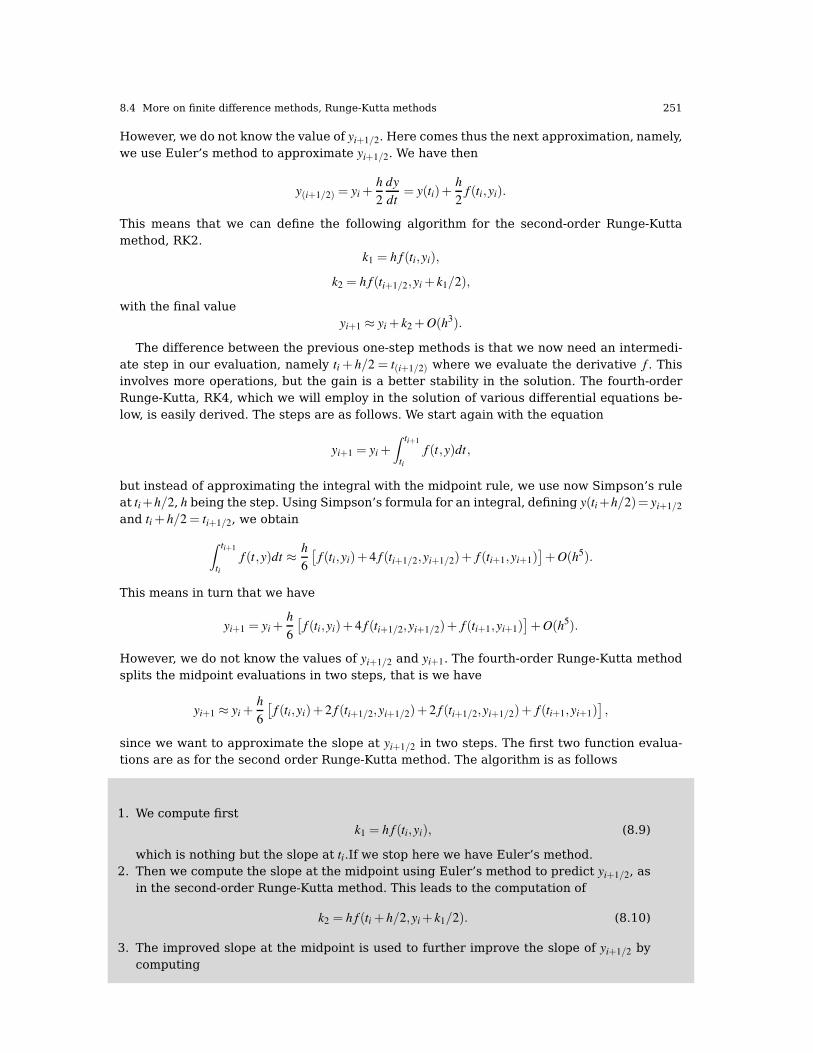
Thus, the algorithm consists in first calculating k1 with ti, y1 and f as inputs. Thereafter, weincrease the step size by h/2 and calculate k2, then k3 and finally k4. With this caveat, we canthen obtain the new value for the variable y. It results in four function evaluations, but theaccuracy is increased by two orders compared with the second-order Runge-Kutta method.The fourth order Runge-Kutta method has a global truncation error which goes like O(h4).Fig. 8.1 gives a geometrical interpretation of the fourth-order Runge-Kutta method.

!

y

t

"

ti

yi and k1

yi+1 and k4

yi+1/2 and k2

yi+1/2 and k3

ti+h/2 ti+hFig. 8.1 Geometrical interpretation of the fourth-order Runge-Kutta method. The derivative is evaluated atfour points, once at the intial point, twice at the trial midpoint and once at the trial endpoint. These fourderivatives constitute one Runge-Kutta step resulting in the final value for yi+1 = yi+1/6(k1 +2k2 +2k3 + k4).

8.5 Adaptive Runge-Kutta and multistep methods 253

8.5 Adaptive Runge-Kutta and multistep methods

In case the function to integrate varies slowly or fast in different integration domains, adap-tive methods are normally used. One strategy is always to decrease the step size. As we haveseen earlier, this leads to more computations and may eventually even lead to the loss ofnumerical precision. An alternative is to use higher-order Runge-Kutta methods for example.However, this leads again to more cycles, furthermore, there is no guarantee that higher-order leads to an improved error, see for example the discussions in Ref. [42]

Assume the exact result is y and that we are using a Runge-Kutta method of order M.Suppose we run two calculations, one with a step length h (which we will label y1) and onewith step length h/2 (labelled y2). The exact solution in terms of y1 is

y= y1 +ChM+1 +O(hM+2),

where C is some constant and

y= y2 + 2C(h/2)M+1+O(hM+2).

Note that we need to perform two calculations in the last equation, one for each intervaldefined by h/2.calculate two halves in the last equation. The difference between the twosolutions is then

|y1! y2|=ChM+1(1! 12M

),

from which we can define the constant C as

C =|y1! y2|

(1! 2!M)hM+1 . (8.14)

We rewrite then the exact solution in terms of a quantity ε

y= y2 + ε+O((h)M+2),

with

ε =|y1! y2|2M! 1

.

If we employ our fourth-order Runge-Kutta scheme, we have

y= y2 + ε+O(h6),

with

ε =|y1! y2|

15.

The estimate is one order higher than the original Runge-Kutta method to fourth order. Butthis method is normally rather inefficient since it requires a lot of computations. We solvetypically the equation three times at each time step. However, we can compare the estimateε with some by us given accuracy ξ say for example ξ = 10!8. We can then ask the followingquestion: what is, with a given y j and t j, the largest possible step size h that leads to an errorbelow ξ? We want

ChM+1 % ξ ,

which leads to, using Eq. (8.14),

!hh

"M+1 |y1! y2|(1! 2!M)

% ξ ,


meaning that we can define this optimal step length as

h= h!ξε

"1/(M+1).

Using this equation, we can design the following algorithm:

• If the two answers are close, use the current value for the step length h.• If ε > ξ we need to decrease the step size in the next time step.• If ε < ξ we need to increase the step size in the next time step.

At each step, two different approximations for the solution are made and compared. If thetwo answers are in close agreement, the approximation is accepted. If the two answers donot agree to a specified accuracy, the step size is reduced. If the answers agree to moresignificant digits than required, the step size is increased. Even though this algorithm israther simple to implement, it requires unnecessarily many computations.

It is possible to reduce the number of operations by combining Runge-Kutta algorithmsof different orders. A much used algorithm is the so-called Runge-Kutta-Fehlberg algorithmwhich uses a combination of fourth and fifth order Runge-Kutta methods, normally abbrevi-ated to RKF45. Without going into much details, the philosophy of such methods consists inevaluating the function f such that the function values can be used for both the fourth orderand the fifth order method, avoiding thereby additional computations. The RKF45 methodrequires at each step the computations of the following six values

k1 = h f (tk,yk),

k2 = h f (tk+14h,yk+

14k1),

k3 = h f (tk+38h,yk+

332k1 +

932k2),

k4 = h f (tk+1213h,yk+

19322197

k1 +72002197

k2 +72962197

k3),

k5 = h f (tk+ h,yk+439216k1! 8k2 +

3680513 k3 +

8454104k4),

and

k6 = h f (tk+12h,yk!

827k1 + 2k2!

35442565

k2 +18594104

k4!+1140k5).

Then an approximation to the solution of the ordinary differential equation is made usinga Runge-Kutta method of order four:

yk+1 = yk+25

216k1 +

14082565

k3 +21974101

k4!15k5,

where the four function values k1 , k3 , k4 , and k5 are used. Notice that k2 is not used here.A better value for the solution is determined using a Runge-Kutta method of order five asfollows

zk+1 = yk+16135

k1 +6656

12825k3 +

2856156430

k4!9

50k5 +

255k6.

The optimal time step αh is then determined by

α =

!ξh

2|zk+1! yk+1|

"1/4,

8.6 Physics examples 255

with ξ our defined tolerance. For more details behind the derivation of this method, see forexample Ref. [42].

8.6 Physics examples

8.6.1 Ideal harmonic oscillations

Our first example is the classical case of simple harmonic oscillations, namely a block slidingon a horizontal frictionless surface. The block is tied to a wall with a spring, portrayed in e.g.,Fig. 8.2. If the spring is not compressed or stretched too far, the force on the block at a givenposition x is

F =!kx.

x

km v

Fig. 8.2 Block tied to a wall with a spring tension acting on it.

The negative sign means that the force acts to restore the object to an equilibrium position.Newton’s equation of motion for this idealized system is then

md2xdt2

=!kx,

or we could rephrase it asd2xdt2

=!kmx=!ω2

0x, (8.15)

with the angular frequency ω20 = k/m.

The above differential equation has the advantage that it can be solved analytically withsolutions on the form

x(t) = Acos(ω0t+ν),

where A is the amplitude and ν the phase constant. This provides in turn an important test forthe numerical solution and the development of a program for more complicated cases whichcannot be solved analytically.


As mentioned earlier, in certain cases it is possible to rewrite a second-order differentialequation as two coupled first-order differential equations. With the position x(t) and the ve-locity v(t) = dx/dt we can reformulate Newton’s equation in the following way

dx(t)dt

= v(t),

anddv(t)dt

=!ω20x(t).

We are now going to solve these equations using the Runge-Kutta method to fourth orderdiscussed previously. Before proceeding however, it is important to note that in addition tothe exact solution, we have at least two further tests which can be used to check our solution.

Since functions like cos are periodic with a period 2π , then the solution x(t) has also to beperiodic. This means that

x(t+T ) = x(t),

with T the period defined as

T =2πω0

=2π(k/m

.

Observe that T depends only on k/m and not on the amplitude of the solution or the con-stant ν.

In addition to the periodicity test, the total energy has also to be conserved.Suppose we choose the initial conditions

x(t = 0) = 1 m v(t = 0) = 0 m/s,

meaning that block is at rest at t = 0 but with a potential energy

E0 =12kx(t = 0)2 =

12k.

The total energy at any time t has however to be conserved, meaning that our solution has tofulfill the condition

E0 =12kx(t)2 +

12mv(t)2.

An algorithm which implements these equations is included below.

1. Choose the initial position and speed, with the most common choice v(t = 0) = 0 andsome fixed value for the position. Since we are going to test our results against theperiodicity requirement, it is convenient to set the final time equal t f = 2π , where wechoose k/m = 1. The initial time is set equal to ti = 0. You could alternatively read inthe ratio k/m.

2. Choose the method you wish to employ in solving the problem. In the enclosed pro-gram we have chosen the fourth-order Runge-Kutta method. Subdivide the time in-terval [ti, t f ] into a grid with step size

h=t f ! tiN

,

where N is the number of mesh points.3. Calculate now the total energy given by


E0 =12kx(t = 0)2 =

12k.

and use this when checking the numerically calculated energy from the Runge-Kuttaiterations.

4. The Runge-Kutta method is used to obtain xi+1 and vi+1 starting from the previousvalues xi and vi..

5. When we have computed x(v)i+1 we upgrade ti+1 = ti+ h.6. This iterative process continues till we reach the maximum time t f = 2π .7. The results are checked against the exact solution. Furthermore, one has to check

the stability of the numerical solution against the chosen number of mesh points N.

8.6.1.1 Program to solve the differential equations for a sliding block

The program which implements the above algorithm is presented here, with a corresponding

http://folk.uio.no/mhjensen/compphys/programs/chapter08/cpp/program1.cpp

/* This program solves Newton's equation for a block sliding on ahorizontal frictionless surface. The block is tied to a wall with aspring, and Newton's equation takes the form m d^2x/dt^2 =-kx withk the spring tension and m the mass of the block. The angularfrequency is omega^2 = k/m and we set it equal 1 in this example

program.

Newton's equation is rewritten as two coupled differentialequations, one for the position x and one for the velocity vdx/dt = v and dv/dt = -x when we set k/m=1

We use therefore a two-dimensional array to represent x and vas functions of t y[0] == x y[1] == v dy[0]/dt = v dy[1]/dt =-x

The derivatives are calculated by the user defined function

derivatives.

The user has to specify the initial velocity (usually v_0=0)the number of steps and the initial position. In theprogramme below we fix the time interval [a,b] to [0,2*pi].

*/ #include <cmath> #include <iostream> #include <fstream> #include<iomanip> #include "lib.h" using namespace std; // output file asglobal variable ofstream ofile; // function declarations voidderivatives(double, double *, double *); void initialise ( double&,double&, int&); void output( double, double *, double); voidrunge_kutta_4(double *, double *, int, double, double, double *,

void (*)(double, double *, double *));

int main(int argc, char* argv[]) { // declarations of variablesdouble *y, *dydt, *yout, t, h, tmax, E0; double initial_x,initial_v; int i, number_of_steps, n; char *outfilename; // Readin output file, abort if there are too few command-line arguments

if( argc <= 1 ){ cout << "Bad Usage: " << argv[0] << " read alsooutput file on same line" << endl; exit(1); } else{outfilename=argv[1]; } ofile.open(outfilename); // this is the

number of differential equations n = 2; // allocate space in


memory for the arrays containing the derivatives dydt = newdouble[n]; y = new double[n]; yout = new double[n]; // read in

the initial position, velocity and number of steps initialise(initial_x, initial_v, number_of_steps); // setting initialvalues, step size and max time tmax h = 4.*acos(-1.)/( (double)number_of_steps); // the step size tmax = h*number_of_steps; //the final time y[0] = initial_x; // initial position y[1] =initial_v; // initial velocity t=0.; // initial time E0 =

0.5*y[0]*y[0]+0.5*y[1]*y[1]; // the initial total energy // nowwe start solving the differential equations using the RK4 methodwhile (t <= tmax){ derivatives(t, y, dydt); // initialderivatives runge_kutta_4(y, dydt, n, t, h, yout, derivatives);for (i = 0; i < n; i++) { y[i] = yout[i]; } t += h; output(t,

y, E0); // write to file } delete [] y; delete [] dydt; delete[] yout; ofile.close(); // close output file return 0; } // End

of main function

// Read in from screen the number of steps, // initial position andinitial speed void initialise (double& initial_x, double&

initial_v, int& number_of_steps) { cout << "Initial position = ";cin >> initial_x; cout << "Initial speed = "; cin >> initial_v;cout << "Number of steps = "; cin >> number_of_steps; } // end of

function initialise

// this function sets up the derivatives for this special case void

derivatives(double t, double *y, double *dydt) { dydt[0]=y[1]; //derivative of x dydt[1]=-y[0]; // derivative of v } // end of

function derivatives

// function to write out the final results void output(double t,double *y, double E0) { ofile << setiosflags(ios::showpoint |

ios::uppercase); ofile << setw(15) << setprecision(8) << t; ofile<< setw(15) << setprecision(8) << y[0]; ofile << setw(15) <<setprecision(8) << y[1]; ofile << setw(15) << setprecision(8) <<cos(t); ofile << setw(15) << setprecision(8) <<0.5*y[0]*y[0]+0.5*y[1]*y[1]-E0 << endl; } // end of function

output

/* This function upgrades a function y (input as a pointer) andreturns the result yout, also as a pointer. Note that thesevariables are declared as arrays. It also receives as input thestarting value for the derivatives in the pointer dydx. It receives

also the variable n which represents the number of differentialequations, the step size h and the initial value of x. It receivesalso the name of the function *derivs where the given derivative iscomputed */ void runge_kutta_4(double *y, double *dydx, int n,double x, double h, double *yout, void (*derivs)(double, double *,double *)) { int i; double xh,hh,h6; double *dym, *dyt, *yt; //

allocate space for local vectors dym = new double [n]; dyt = newdouble [n]; yt = new double [n]; hh = h*0.5; h6 = h/6.; xh =x+hh; for (i = 0; i < n; i++) { yt[i] = y[i]+hh*dydx[i]; }(*derivs)(xh,yt,dyt); // computation of k2, eq. 3.60 for (i = 0;i < n; i++) { yt[i] = y[i]+hh*dyt[i]; } (*derivs)(xh,yt,dym); //computation of k3, eq. 3.61 for (i=0; i < n; i++) { yt[i] =

y[i]+h*dym[i]; dym[i] += dyt[i]; } (*derivs)(x+h,yt,dyt); //computation of k4, eq. 3.62 // now we upgrade y in the array youtfor (i = 0; i < n; i++){ yout[i] =y[i]+h6*(dydx[i]+dyt[i]+2.0*dym[i]); } delete []dym; delete []

dyt; delete [] yt; } // end of function Runge-kutta 4


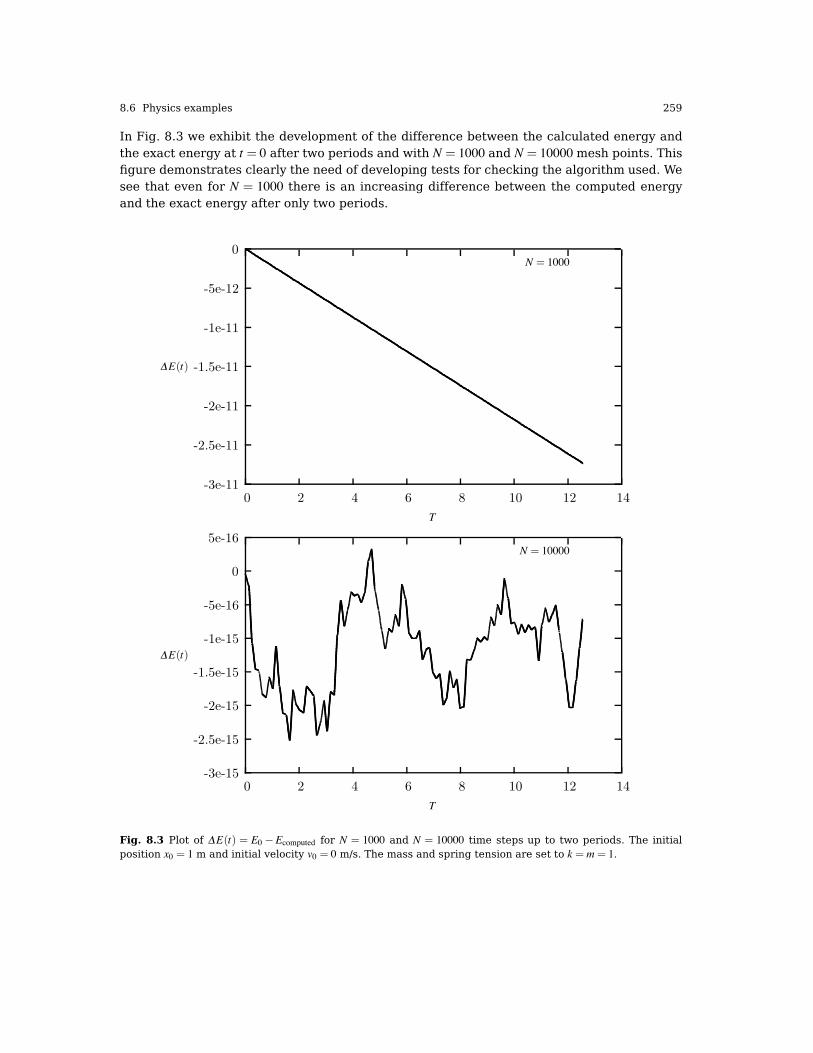
In Fig. 8.3 we exhibit the development of the difference between the calculated energy andthe exact energy at t = 0 after two periods and with N = 1000 and N = 10000 mesh points. Thisfigure demonstrates clearly the need of developing tests for checking the algorithm used. Wesee that even for N = 1000 there is an increasing difference between the computed energyand the exact energy after only two periods.

-3e-11

-2.5e-11

-2e-11

-1.5e-11

-1e-11

-5e-12

0

0 2 4 6 8 10 12 14

ΔE(t)

T

N = 1000

-3e-15

-2.5e-15

-2e-15

-1.5e-15

-1e-15

-5e-16

0

5e-16

0 2 4 6 8 10 12 14

ΔE(t)

T

N = 10000

Fig. 8.3 Plot of ΔE(t) = E0 !Ecomputed for N = 1000 and N = 10000 time steps up to two periods. The initialposition x0 = 1 m and initial velocity v0 = 0 m/s. The mass and spring tension are set to k =m= 1.


8.6.2 Damping of harmonic oscillations and external forces

Most oscillatory motion in nature does decrease until the displacement becomes zero. We callsuch a motion for damped and the system is said to be dissipative rather than conservative.Considering again the simple block sliding on a plane, we could try to implement such adissipative behavior through a drag force which is proportional to the first derivative of x,i.e., the velocity. We can then expand Eq. (8.15) to

d2xdt2

=!ω20x!ν

dxdt

, (8.16)

where ν is the damping coefficient, being a measure of the magnitude of the drag term.We could however counteract the dissipative mechanism by applying e.g., a periodic exter-

nal forceF(t) = Bcos(ωt),

and we rewrite Eq. (8.16) asd2xdt2

=!ω20x!ν

dxdt

+F(t). (8.17)

Although we have specialized to a block sliding on a surface, the above equations arerather general for quite many physical systems.

If we replace x by the charge Q, ν with the resistance R, the velocity with the current I,the inductance L with the mass m, the spring constant with the inverse capacitanceC and theforce F with the voltage drop V , we rewrite Eq. (8.17) as

Ld2Qdt2

+QC+R

dQdt

=V (t). (8.18)

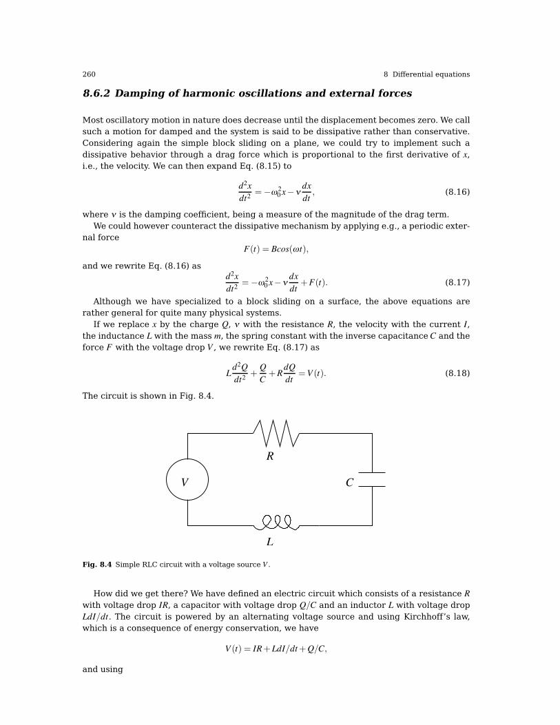
The circuit is shown in Fig. 8.4.

V

L

C

R

Fig. 8.4 Simple RLC circuit with a voltage source V .

How did we get there? We have defined an electric circuit which consists of a resistance Rwith voltage drop IR, a capacitor with voltage drop Q/C and an inductor L with voltage dropLdI/dt. The circuit is powered by an alternating voltage source and using Kirchhoff’s law,which is a consequence of energy conservation, we have

V (t) = IR+LdI/dt+Q/C,

and using


I =dQdt

,

we arrive at Eq. (8.18).This section was meant to give you a feeling of the wide range of applicability of the

methods we have discussed. However, before leaving this topic entirely, we’ll dwelve into theproblems of the pendulum, from almost harmonic oscillations to chaotic motion!

8.6.3 The pendulum, a nonlinear differential equation

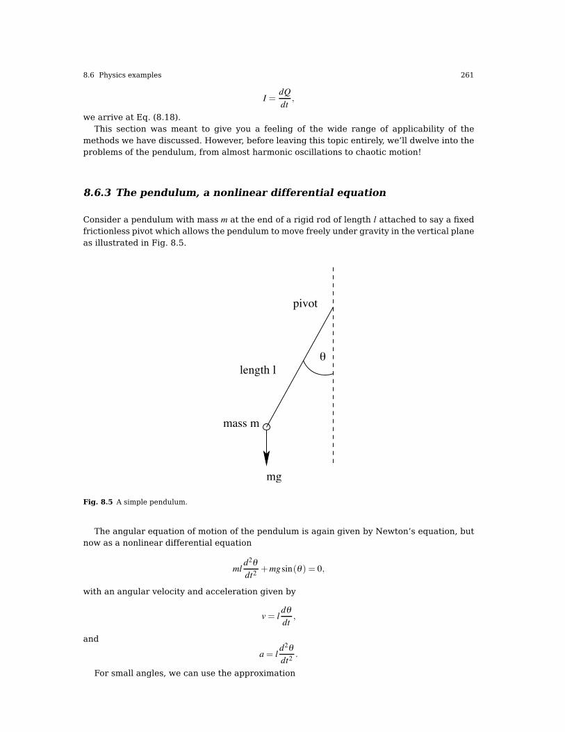
Consider a pendulum with mass m at the end of a rigid rod of length l attached to say a fixedfrictionless pivot which allows the pendulum to move freely under gravity in the vertical planeas illustrated in Fig. 8.5.

mg

mass m

length l

pivot

θ

Fig. 8.5 A simple pendulum.

The angular equation of motion of the pendulum is again given by Newton’s equation, butnow as a nonlinear differential equation

mld2θdt2

+mgsin(θ ) = 0,

with an angular velocity and acceleration given by

v= ldθdt

,

and

a= ld2θdt2

.

For small angles, we can use the approximation


sin(θ )# θ .

and rewrite the above differential equation as

d2θdt2

=!glθ ,

which is exactly of the same form as Eq. (8.15). We can thus check our solutions for smallvalues of θ against an analytical solution. The period is now

T =2π(l/g

.

We do however expect that the motion will gradually come to an end due a viscous dragtorque acting on the pendulum. In the presence of the drag, the above equation becomes

mld2θdt2

+νdθdt

+mgsin(θ ) = 0,

where ν is now a positive constant parameterizing the viscosity of the medium in question.In order to maintain the motion against viscosity, it is necessary to add some external drivingforce. We choose here, in analogy with the discussion about the electric circuit, a periodicdriving force. The last equation becomes then

mld2θdt2

+νdθdt

+mgsin(θ ) = Acos(ωt), (8.19)

with A and ω two constants representing the amplitude and the angular frequency respec-tively. The latter is called the driving frequency.

If we now define the natural frequency

ω0 =(g/l,

the so-called natural frequency and the new dimensionless quantities

t = ω0t,

with the dimensionless driving frequency

ω =ωω0

,

and introducing the quantity Q, called the quality factor,

Q=mgω0ν

,

and the dimensionless amplitude

A=Amg

we can rewrite Eq. (8.19) as

d2θdt2

+1Qdθdt

+ sin(θ ) = Acos(ω t).

This equation can in turn be recast in terms of two coupled first-order differential equationsas follows

8.7 Physics Project: the pendulum 263

dθdt

= v,

anddvdt

=!vQ! sin(θ )+ Acos(ω t).

These are the equations to be solved. The factor Q represents the number of oscillationsof the undriven system that must occur before its energy is significantly reduced due to theviscous drag. The amplitude A is measured in units of the maximum possible gravitationaltorque while ω is the angular frequency of the external torque measured in units of thependulum’s natural frequency.

8.7 Physics Project: the pendulum

8.7.1 Analytic results for the pendulum

Although the solution to the equations for the pendulum can only be obtained through nu-merical efforts, it is always useful to check our numerical code against analytic solutions. Forsmall angles θ , we have sin(θ )# θ and our equations become

dθdt

= v,

anddvdt

=!vQ!θ + Acos(ω t).

These equations are linear in the angle θ and are similar to those of the sliding block or theRLC circuit. With given initial conditions v0 and θ0 they can be solved analytically to yield

θ (t) =)θ0! A(1!ω2)

(1!ω2)2+ω2/Q2

*e!τ/2Qcos(

+1! 1

4Q2 τ)

+)v0 +

θ02Q !

A(1!3ω2)/2Q(1!ω2)2+ω2/Q2

*e!τ/2Qsin(

+1! 1

4Q2 τ)+A(1!ω2)cos(ωτ)+ ω

Q sin(ωτ)(1!ω2)2+ω2/Q2 ,

and

v(t) =)v0! Aω2/Q

(1!ω2)2+ω2/Q2

*e!τ/2Qcos(

+1! 1

4Q2 τ)

!)θ0 +

v02Q !

A[(1!ω2)!ω2/Q2](1!ω2)2+ω2/Q2

*e!τ/2Qsin(

+1! 1

4Q2 τ)+ωA[!(1!ω2)sin(ωτ)+ ω

Q cos(ωτ)](1!ω2)2+ω2/Q2 ,

with Q > 1/2. The first two terms depend on the initial conditions and decay exponentiallyin time. If we wait long enough for these terms to vanish, the solutions become independentof the initial conditions and the motion of the pendulum settles down to the following simpleorbit in phase space

θ (t) =A(1! ω2)cos(ωτ)+ ω

Q sin(ωτ)(1! ω2)2 + ω2/Q2 ,

and

v(t) =ωA[!(1! ω2)sin(ωτ)+ ω

Qcos(ωτ)](1! ω2)2 + ω2/Q2 ,

tracing the closed phase-space curve


!θA

"2+

!vωA

"2= 1

with

A=A(

(1! ω2)2 + ω2/Q2.

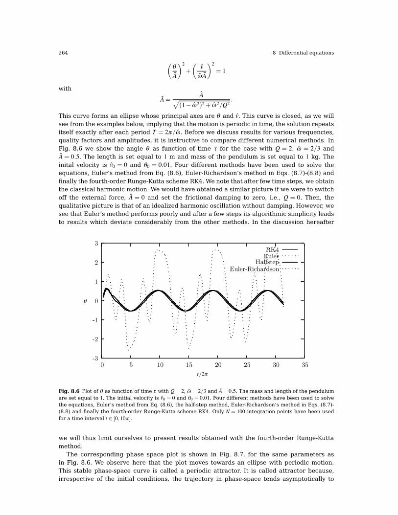
This curve forms an ellipse whose principal axes are θ and v. This curve is closed, as we willsee from the examples below, implying that the motion is periodic in time, the solution repeatsitself exactly after each period T = 2π/ω. Before we discuss results for various frequencies,quality factors and amplitudes, it is instructive to compare different numerical methods. InFig. 8.6 we show the angle θ as function of time τ for the case with Q = 2, ω = 2/3 andA = 0.5. The length is set equal to 1 m and mass of the pendulum is set equal to 1 kg. Theinital velocity is v0 = 0 and θ0 = 0.01. Four different methods have been used to solve theequations, Euler’s method from Eq. (8.6), Euler-Richardson’s method in Eqs. (8.7)-(8.8) andfinally the fourth-order Runge-Kutta scheme RK4. We note that after few time steps, we obtainthe classical harmonic motion. We would have obtained a similar picture if we were to switchoff the external force, A = 0 and set the frictional damping to zero, i.e., Q = 0. Then, thequalitative picture is that of an idealized harmonic oscillation without damping. However, wesee that Euler’s method performs poorly and after a few steps its algorithmic simplicity leadsto results which deviate considerably from the other methods. In the discussion hereafter

-3

-2

-1

0

1

2

3

0 5 10 15 20 25 30 35

θ

t/2π

RK4Euler

HalfstepEuler-Richardson

Fig. 8.6 Plot of θ as function of time τ with Q= 2, ω = 2/3 and A= 0.5. The mass and length of the pendulumare set equal to 1. The initial velocity is v0 = 0 and θ0 = 0.01. Four different methods have been used to solvethe equations, Euler’s method from Eq. (8.6), the half-step method, Euler-Richardson’s method in Eqs. (8.7)-(8.8) and finally the fourth-order Runge-Kutta scheme RK4. Only N = 100 integration points have been usedfor a time interval t & [0,10π ].

we will thus limit ourselves to present results obtained with the fourth-order Runge-Kuttamethod.

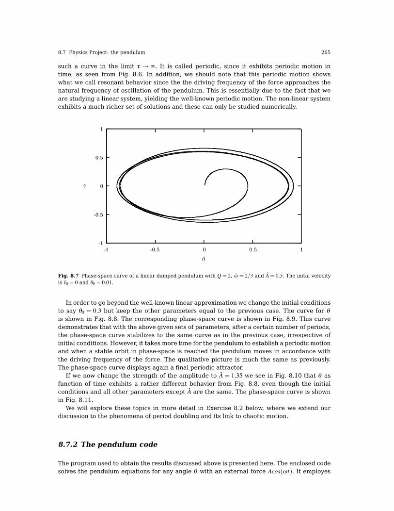
The corresponding phase space plot is shown in Fig. 8.7, for the same parameters asin Fig. 8.6. We observe here that the plot moves towards an ellipse with periodic motion.This stable phase-space curve is called a periodic attractor. It is called attractor because,irrespective of the initial conditions, the trajectory in phase-space tends asymptotically to


such a curve in the limit τ ' ∞. It is called periodic, since it exhibits periodic motion intime, as seen from Fig. 8.6. In addition, we should note that this periodic motion showswhat we call resonant behavior since the the driving frequency of the force approaches thenatural frequency of oscillation of the pendulum. This is essentially due to the fact that weare studying a linear system, yielding the well-known periodic motion. The non-linear systemexhibits a much richer set of solutions and these can only be studied numerically.

-1

-0.5

0

0.5

1

-1 -0.5 0 0.5 1

v

θ

Fig. 8.7 Phase-space curve of a linear damped pendulum with Q= 2, ω = 2/3 and A = 0.5. The inital velocityis v0 = 0 and θ0 = 0.01.

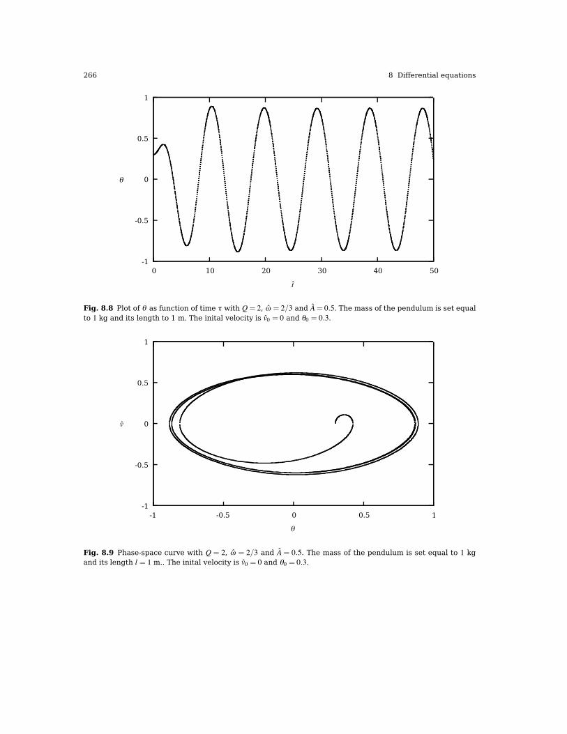
In order to go beyond the well-known linear approximation we change the initial conditionsto say θ0 = 0.3 but keep the other parameters equal to the previous case. The curve for θis shown in Fig. 8.8. The corresponding phase-space curve is shown in Fig. 8.9. This curvedemonstrates that with the above given sets of parameters, after a certain number of periods,the phase-space curve stabilizes to the same curve as in the previous case, irrespective ofinitial conditions. However, it takes more time for the pendulum to establish a periodic motionand when a stable orbit in phase-space is reached the pendulum moves in accordance withthe driving frequency of the force. The qualitative picture is much the same as previously.The phase-space curve displays again a final periodic attractor.

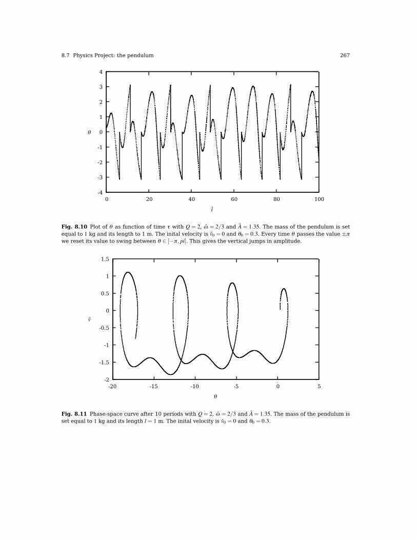
If we now change the strength of the amplitude to A = 1.35 we see in Fig. 8.10 that θ asfunction of time exhibits a rather different behavior from Fig. 8.8, even though the initialconditions and all other parameters except A are the same. The phase-space curve is shownin Fig. 8.11.

We will explore these topics in more detail in Exercise 8.2 below, where we extend ourdiscussion to the phenomena of period doubling and its link to chaotic motion.

8.7.2 The pendulum code

The program used to obtain the results discussed above is presented here. The enclosed codesolves the pendulum equations for any angle θ with an external force Acos(ωt). It employes


-1

-0.5

0

0.5

1

0 10 20 30 40 50

θ

t

Fig. 8.8 Plot of θ as function of time τ with Q= 2, ω = 2/3 and A= 0.5. The mass of the pendulum is set equalto 1 kg and its length to 1 m. The inital velocity is v0 = 0 and θ0 = 0.3.

-1

-0.5

0

0.5

1

-1 -0.5 0 0.5 1

v

θ

Fig. 8.9 Phase-space curve with Q = 2, ω = 2/3 and A = 0.5. The mass of the pendulum is set equal to 1 kgand its length l = 1 m.. The inital velocity is v0 = 0 and θ0 = 0.3.


-4

-3

-2

-1

0

1

2

3

4

0 20 40 60 80 100

θ

t

Fig. 8.10 Plot of θ as function of time τ with Q = 2, ω = 2/3 and A = 1.35. The mass of the pendulum is setequal to 1 kg and its length to 1 m. The inital velocity is v0 = 0 and θ0 = 0.3. Every time θ passes the value ±πwe reset its value to swing between θ & [!π , pi]. This gives the vertical jumps in amplitude.

-2

-1.5

-1

-0.5

0

0.5

1

1.5

-20 -15 -10 -5 0 5

v

θ

Fig. 8.11 Phase-space curve after 10 periods with Q= 2, ω = 2/3 and A= 1.35. The mass of the pendulum isset equal to 1 kg and its length l = 1 m. The inital velocity is v0 = 0 and θ0 = 0.3.


several methods for solving the two coupled differential equations, from Euler’s method toadaptive size methods coupled with fourth-order Runge-Kutta. It is straightforward to applythis program to other systems which exhibit harmonic oscillations or change the functionalform of the external force.

We have also introduced a class where we define various methods for solving ordinary andcoupled first order differential equations. This is done via the . classpendulum. This methodsaccess variables which belong only to this particular class via the private declaration. Assuch, the methods we list here can easily be reused by other types of ordinary differentialequations. In the code below, we list only the fourth order Runge Kutta method, which wasused to generate the above figures. For the full code see programs/chapter08/program2.cpp.

http://folk.uio.no/mhjensen/compphys/programs/chapter08/cpp/program2.cpp

#include <stdio.h> include <iostream.h> include <math.h> include

#<fstream.h> /* Different methods for solving ODEs are presented We#are solving the following eqation:

m*l*(phi)'' + viscosity*(phi)' + m*g*sin(phi) = A*cos(omega*t)

If you want to solve similar equations with other values you have

to rewrite the methods 'derivatives' and 'initialise' and changethe variables in the private part of the class Pendulum

At first we rewrite the equation using the following definitions:

omega_0 = sqrt(g*l) t_roof = omega_0*t omega_roof = omega/omega_0 Q= (m*g)/(omega_0*reib) A_roof = A/(m*g)

and we get a dimensionless equation

(phi)'' + 1/Q*(phi)' + sin(phi) = A_roof*cos(omega_roof*t_roof)

This equation can be written as two equations of first order:

(phi)' = v (v)' = -v/Q - sin(phi) +A_roof*cos(omega_roof*t_roof)

All numerical methods are applied to the last two equations. The

algorithms are taken from the book "An introduction to computersimulation methods" */

class pendelum { private: double Q, A_roof, omega_0, omega_roof,g;// double y[2]; //for the initial-values of phi and v int n; //how many steps double delta_t,delta_t_roof; // Definition of

methods to solve ODEs public: void

derivatives(double,double*,double*); void initialise(); void

euler(); void euler_cromer(); void midpoint(); void

euler_richardson(); void half_step(); void rk2();//runge-kutta-second-order void

rk4_step(double,double*,double*,double); // we need it infunction rk4() and asc() void rk4(); //runge-kutta-fourth-ordervoid asc(); //runge-kutta-fourth-order with adaptive stepsizecontrol };

// This function defines the particular coupled first order ODEs void

pendelum::derivatives(double t, double* in, double* out) { /* Here weare calculating the derivatives at (dimensionless) time t 'in' arethe values of phi and v, which are used for the calculation Theresults are given to 'out' */

out[0]=in[1]; //out[0] = (phi)' = v if(Q)


out[1]=-in[1]/((double)Q)-sin(in[0])+A_roof*cos(omega_roof*t);//out[1] = (phi)'' else

out[1]=-sin(in[0])+A_roof*cos(omega_roof*t); //out[1] = (phi)'' }// Here we define all input parameters. void pendelum::initialise(){ double m,l,omega,A,viscosity,phi_0,v_0,t_end; cout<<"Solving thedifferential eqation of the pendulum!\n"; cout<<"We have a pendulumwith mass m, length l. Then we have a periodic force with amplitudeA and omega\n"; cout<<"Furthermore there is a viscous drag

coefficient.\n"; cout<<"The initial conditions at t=0 are phi_0 andv_0\n"; cout<<"Mass m: "; cin>>m; cout<<"length l: "; cin>>l;cout<<"omega of the force: "; cin>>omega; cout<<"amplitude of theforce: "; cin>>A; cout<<"The value of the viscous drag constant(viscosity): "; cin>>viscosity; cout<<"phi_0: "; cin>>y[0];

cout<<"v_0: "; cin>>y[1]; cout<<"Number of time steps orintegration steps:"; cin>>n; cout<<"Final time steps as multiplumof pi:"; cin>>t_end; t_end *= acos(-1.); g=9.81; // We need thefollowing values: omega_0=sqrt(g/((double)l)); // omega of thependulum if (viscosity) Q= m*g/((double)omega_0*viscosity); elseQ=0; //calculating Q A_roof=A/((double)m*g);

omega_roof=omega/((double)omega_0);delta_t_roof=omega_0*t_end/((double)n); //delta_t without dimensiondelta_t=t_end/((double)n); } // fourth order Run void

pendelum::rk4_step(double t,double *yin,double *yout,double delta_t){ /* The function calculates one step offourth-order-runge-kutta-method We will need it for the normal

fourth-order-Runge-Kutta-method and for RK-method with adaptivestepsize control

The function calculates the value of y(t + delta_t) usingfourth-order-RK-method Input: time t and the stepsize delta_t,yin (values of phi and v at time t) Output: yout (values of phi

and v at time t+delta_t)

*/ double k1[2],k2[2],k3[2],k4[2],y_k[2]; // Calculation of k1derivatives(t,yin,yout); k1[1]=yout[1]*delta_t;k1[0]=yout[0]*delta_t; y_k[0]=yin[0]+k1[0]*0.5;

y_k[1]=yin[1]+k1[1]*0.5; /*Calculation of k2 */derivatives(t+delta_t*0.5,y_k,yout); k2[1]=yout[1]*delta_t;k2[0]=yout[0]*delta_t; y_k[0]=yin[0]+k2[0]*0.5;y_k[1]=yin[1]+k2[1]*0.5; /* Calculation of k3 */derivatives(t+delta_t*0.5,y_k,yout); k3[1]=yout[1]*delta_t;k3[0]=yout[0]*delta_t; y_k[0]=yin[0]+k3[0]; y_k[1]=yin[1]+k3[1];

/*Calculation of k4 */ derivatives(t+delta_t,y_k,yout);k4[1]=yout[1]*delta_t; k4[0]=yout[0]*delta_t; /*Calculation ofnew values of phi and v */yout[0]=yin[0]+1.0/6.0*(k1[0]+2*k2[0]+2*k3[0]+k4[0]);yout[1]=yin[1]+1.0/6.0*(k1[1]+2*k2[1]+2*k3[1]+k4[1]); }

void pendelum::rk4() { /*We are using thefourth-order-Runge-Kutta-algorithm We have to calculate theparameters k1, k2, k3, k4 for v and phi, so we use to arraysk1[2] and k2[2] for this k1[0], k2[0] are the parameters for phi,k1[1], k2[1] are the parameters for v */

int i; double t_h; double yout[2],y_h[2];//k1[2],k2[2],k3[2],k4[2],y_k[2];

t_h=0; y_h[0]=y[0]; //phi y_h[1]=y[1]; //v ofstreamfout("rk4.out"); fout.setf(ios::scientific); fout.precision(20);for(i=1; i<=n; i++){ rk4_step(t_h,y_h,yout,delta_t_roof);

fout<<i*delta_t<<"\t\t"<<yout[0]<<"\t\t"<<yout[1]<<"\n";


t_h+=delta_t_roof; y_h[0]=yout[0]; y_h[1]=yout[1]; }fout.close; }

int main() { pendelum testcase; testcase.initialise();testcase.rk4(); return 0; } // end of main function

8.8 Exercises

8.1. In the pendulum example we rewrote the equations as two differential equations in termsof so-called dimensionless variables. One should always do that. There are at least two goodreasons for doing this.

• By rewriting the equations as dimensionless ones, the program will most likely be easier toread, with hopefully a better possibility of spotting eventual errors. In addtion, the variousconstants which are pulled out of the equations in the process of rendering the equationsdimensionless, are reintroduced at the end of the calculation. If one of these constants isnot correctly defined, it is easier to spot an eventual error.

• In many physics applications, variables which enter a differential equation, may differby orders of magnitude. If we were to insist on not using dimensionless quantities, suchdifferences can cause serious problems with respect to loss of numerical precision.

An example which demonstrates these features is the set of equations for gravitationalequilibrium of a neutron star. We will not solve these equations numerically here, rather, wewill limit ourselves to merely rewriting these equations in a dimensionless form.

The equations for a neutron star

The discovery of the neutron by Chadwick in 1932 prompted Landau to predict the existenceof neutron stars. The birth of such stars in supernovae explosions was suggested by Baadeand Zwicky 1934. First theoretical neutron star calculations were performed by Tolman, Op-penheimer and Volkoff in 1939 and Wheeler around 1960. Bell and Hewish were the first todiscover a neutron star in 1967 as a radio pulsar. The discovery of the rapidly rotating Crabpulsar ( rapidly rotating neutron star) in the remnant of the Crab supernova observed by thechinese in 1054 A.D. confirmed the link to supernovae. Radio pulsars are rapidly rotating withperiods in the range 0.033 s % P% 4.0 s. They are believed to be powered by rotational energyloss and are rapidly spinning down with period derivatives of order P ( 10!12! 10!16. Theirhigh magnetic field B leads to dipole magnetic braking radiation proportional to the magneticfield squared. One estimates magnetic fields of the order of B( 1011! 1013 G. The total num-ber of pulsars discovered so far has just exceeded 1000 before the turn of the millenium andthe number is increasing rapidly.

The physics of compact objects like neutron stars offers an intriguing interplay betweennuclear processes and astrophysical observables, see Refs. [46–48] for further informationand references on the physics of neutron stars. Neutron stars exhibit conditions far fromthose encountered on earth; typically, expected densities ρ of a neutron star interior are ofthe order of 103 or more times the density ρd # 4 ·1011 g/cm3 at ’neutron drip’, the density atwhich nuclei begin to dissolve and merge together. Thus, the determination of an equationof state (EoS) for dense matter is essential to calculations of neutron star properties. TheEoS determines properties such as the mass range, the mass-radius relationship, the crustthickness and the cooling rate. The same EoS is also crucial in calculating the energy releasedin a supernova explosion.

8.8 Exercises 271

Clearly, the relevant degrees of freedom will not be the same in the crust region of a neu-tron star, where the density is much smaller than the saturation density of nuclear matter, andin the center of the star, where density is so high that models based solely on interacting nu-cleons are questionable. Neutron star models including various so-called realistic equationsof state result in the following general picture of the interior of a neutron star. The surfaceregion, with typical densities ρ < 106 g/cm3, is a region in which temperatures and magneticfields may affect the equation of state. The outer crust for 106 g/cm3 < ρ < 4 · 1011g/cm3 is asolid region where a Coulomb lattice of heavy nuclei coexist in β -equilibrium with a relativis-tic degenerate electron gas. The inner crust for 4 ·1011 g/cm3 < ρ < 2 ·1014g/cm3 consists of alattice of neutron-rich nuclei together with a superfluid neutron gas and an electron gas. Theneutron liquid for 2 · 1014 g/cm3 < ρ < 1015g/cm3 contains mainly superfluid neutrons with asmaller concentration of superconducting protons and normal electrons. At higher densities,typically 2! 3 times nuclear matter saturation density, interesting phase transitions from aphase with just nucleonic degrees of freedom to quark matter may take place. Furthermore,one may have a mixed phase of quark and nuclear matter, kaon or pion condensates, hyper-onic matter, strong magnetic fields in young stars etc.

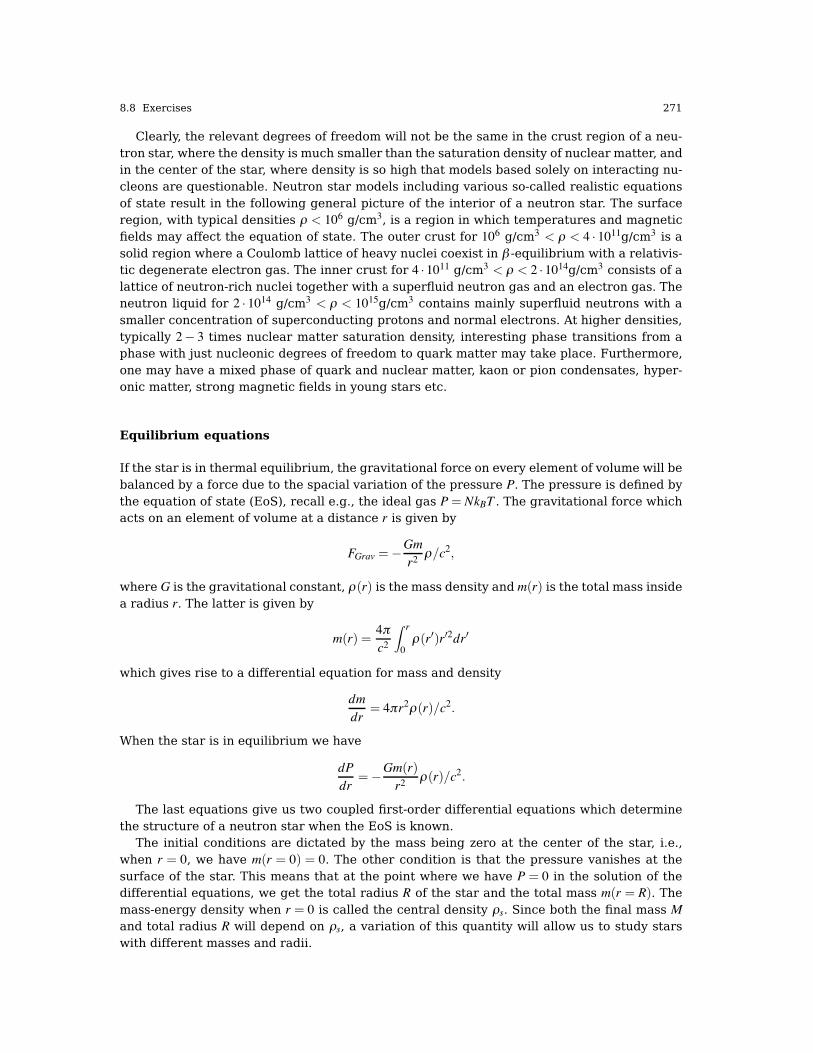
Equilibrium equations

If the star is in thermal equilibrium, the gravitational force on every element of volume will bebalanced by a force due to the spacial variation of the pressure P. The pressure is defined bythe equation of state (EoS), recall e.g., the ideal gas P= NkBT . The gravitational force whichacts on an element of volume at a distance r is given by

FGrav =!Gmr2 ρ/c2,

where G is the gravitational constant, ρ(r) is the mass density and m(r) is the total mass insidea radius r. The latter is given by

m(r) =4πc2

% r

0ρ(r")r"2dr"

which gives rise to a differential equation for mass and density

dmdr

= 4πr2ρ(r)/c2.

When the star is in equilibrium we have

dPdr

=!Gm(r)r2 ρ(r)/c2.

The last equations give us two coupled first-order differential equations which determinethe structure of a neutron star when the EoS is known.

The initial conditions are dictated by the mass being zero at the center of the star, i.e.,when r = 0, we have m(r = 0) = 0. The other condition is that the pressure vanishes at thesurface of the star. This means that at the point where we have P = 0 in the solution of thedifferential equations, we get the total radius R of the star and the total mass m(r = R). Themass-energy density when r = 0 is called the central density ρs. Since both the final mass Mand total radius R will depend on ρs, a variation of this quantity will allow us to study starswith different masses and radii.


Dimensionless equations

When we now attempt the numerical solution, we need however to rescale the equations sothat we deal with dimensionless quantities only. To understand why, consider the value of thegravitational constant G and the possible final mass m(r = R) =MR. The latter is normally ofthe order of some solar massesM), withM)= 1.989*1030 Kg. If we wish to translate the latterinto units of MeV/c2, we will have that MR ( 1060 MeV/c2. The gravitational constant is in unitsof G= 6.67*10!45* hc (MeV/c2)!2. It is then easy to see that including the relevant values forthese quantities in our equations will most likely yield large numerical roundoff errors whenwe add a huge number dP

dr to a smaller number P in order to obtain the new pressure. We listhere the units of the various quantities and in case of physical constants, also their values. Abracketed symbol like [P] stands for the unit of the quantity inside the brackets.

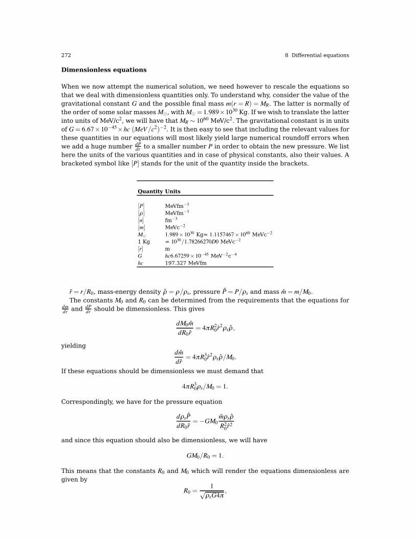
Quantity Units

[P] MeVfm!3

[ρ ] MeVfm!3

[n] fm!3

[m] MeVc!2

M) 1.989*1030 Kg= 1.1157467*1060 MeVc!2

1 Kg = 1030/1.78266270D0 MeVc!2

[r] mG hc6.67259*10!45 MeV!2c!4

hc 197.327 MeVfm

r = r/R0, mass-energy density ρ = ρ/ρs, pressure P= P/ρs and mass m= m/M0.The constants M0 and R0 can be determined from the requirements that the equations for

dmdr and dP

dr should be dimensionless. This gives

dM0mdR0r

= 4πR20r2ρsρ ,

yieldingdmdr

= 4πR30r2ρsρ/M0.

If these equations should be dimensionless we must demand that

4πR30ρs/M0 = 1.

Correspondingly, we have for the pressure equation

dρsPdR0r

=!GM0mρsρR2

0r2

and since this equation should also be dimensionless, we will have

GM0/R0 = 1.

This means that the constants R0 and M0 which will render the equations dimensionless aregiven by

R0 =1+

ρsG4π,

8.8 Exercises 273

and

M0 =4πρs

(+ρsG4π)3 .

However, since we would like to have the radius expressed in units of 10 km, we shouldmultiply R0 by 10!19, since 1 fm = 10!15 m. Similarly, M0 will come in units of MeV/c2, and itis convenient therefore to divide it by the mass of the sun and express the total mass in termsof solar masses M).

The differential equations read then

dPdr

=!mρr2 ,

dmdr

= r2ρ .

In the solution of our problem, we will assume that the mass-energy density is given bya simple parametrization from Bethe and Johnson [49]. This parametrization gives ρ as afunction of the number density n= N/V , with N the total number of baryons in a volume V . Itreads

ρ(n) = 236* n2.54+ nmn, (8.20)

where mn = 938.926MeV/c2, the mass of the neutron (averaged). This means that since[n] =fm!3, we have that the dimension of ρ is [ρ ] =MeV/c2fm!3. Through the thermodynamicrelation

P=!∂E∂V

, (8.21)

where E is the energy in units of MeV/c2 we have

P(n) = n∂ρ(n)∂n

!ρ(n) = 363.44* n2.54.

We see that the dimension of pressure is the same as that of the mass-energy density, i.e.,[P] =MeV/c2fm!3.

Here comes an important point you should observe when solving the two coupled first-order differential equations. When you obtain the new pressure given by

Pnew =dPdr

+Pold,

this comes as a function of r. However, having obtained the new pressure, you will need touse Eq. (8.1) in order to find the number density n. This will in turn allow you to find the newvalue of the mass-energy density ρ(n) at the relevant value of r.

In solving the differential equations for neutron star equilibrium, you should proceed asfollows

1. Make first a dimensional analysis in order to be sure that all equations are really dimen-sionless.

2. Define the constants R0 and M0 in units of 10 km and solar mass M). Find their values.Explain why it is convenient to insert these constants in the final results and not at eachintermediate step.

3. Set up the algorithm for solving these equations and write a main program where thevarious variables are defined.

4. Write thereafter a small function which uses the expressions for pressure and mass-energydensity from Eqs. (8.1) and (8.20).

5. Write then a function which sets up the derivatives

!mρr2 , r2ρ.


6. Employ now the fourth order Runge-Kutta algorithm to obtain new values for the pressureand the mass. Play around with different values for the step size and compare the resultsfor mass and radius.

7. Replace the fourth order Runge-Kutta method with the simple Euler method and comparethe results.

8. Replace the non-relativistic expression for the derivative of the pressure with that fromGeneral Relativity (GR), the so-called Tolman-Oppenheimer-Volkov equation

dPdr

=!(P+ ρ)(r3P+ m)

r2! 2mr,

and solve again the two differential equations.9. Compare the non-relatistic and the GR results by plotting mass and radius as functions of

the central density.

8.2.

mld2θdt2

+mgsin(θ ) = 0,

with an angular velocity and acceleration given by

v= ldθdt

,

and

a= ld2θdt2

.

We do however expect that the motion will gradually come to an end due a viscous dragtorque acting on the pendulum. In the presence of the drag, the above equation becomes

mld2θdt2

+νdθdt

+mgsin(θ ) = 0, (8.22)

where ν is now a positive constant parameterizing the viscosity of the medium in question.In order to maintain the motion against viscosity, it is necessary to add some external drivingforce. We choose here a periodic driving force. The last equation becomes then

mld2θdt2

+νdθdt

+mgsin(θ ) = Asin(ωt), (8.23)

with A and ω two constants representing the amplitude and the angular frequency respec-tively. The latter is called the driving frequency.

1. Rewrite Eqs. (8.22) and (8.23) as dimensionless equations.2. Write then a code which solves Eq. (8.22) using the fourth-order Runge Kutta method.

Perform calculations for at least ten periods with N = 100, N = 1000 and N = 10000 meshpoints and values of ν = 1, ν = 5 and ν = 10. Set l = 1.0 m, g= 1 m/s2 and m= 1 kg. Choose asinitial conditions θ (0) = 0.2 (radians) and v(0) = 0 (radians/s). Make plots of θ (in radians)as function of time and phase space plots of θ versus the velocity v. Check the stability ofyour results as functions of time and number of mesh points. Which case corresponds todamped, underdamped and overdamped oscillatory motion? Comment your results.

3. Now we switch to Eq. (8.23) for the rest of the project. Add an external driving force andset l = g= 1, m= 1, ν = 1/2 and ω = 2/3. Choose as initial conditions θ (0) = 0.2 and v(0) = 0and A = 0.5 and A = 1.2. Make plots of θ (in radians) as function of time for at least 300periods and phase space plots of θ versus the velocity v. Choose an appropriate time step.Comment and explain the results for the different values of A.

8.8 Exercises 275

4. Keep now the constants from the previous exercise fixed but set now A= 1.35, A= 1.44 andA= 1.465. Plot θ (in radians) as function of time for at least 300 periods for these values ofA and comment your results.

5. We want to analyse further these results by making phase space plots of θ versus thevelocity v using only the points where we have ωt = 2nπ where n is an integer. These arenormally called the drive periods. This is an example of what is called a Poincare sectionand is a very useful way to plot and analyze the behavior of a dynamical system. Commentyour results.

8.3. We assume that the orbit of Earth around the Sun is co-planar, and we take this to be thexy-plane. Using Newton’s second law of motion we get the following equations

d2xdt2

=FG,xMEarth

,

andd2ydt2

=FG,yMEarth

,

where FG,x and FG,y are the x and y components of the gravitational force.

a) Rewrite the above second-order ordinary differential equations as a set of coupled first or-der differential equations. Write also these equations in terms of dimensionless variables.As an alternative to the usage of dimensionless variables, you could also use so-calledastronomical units (AU as abbreviation). If you choose the latter set of units, one astro-nomical unit of length, known as 1 AU, is the average distance between the Sun and Earth,that is 1 AU = 1.5* 1011 m. It can also be convenient to use years instead of secondssince years match better the solar system. The mass of the Sun is Msun = M) = 2* 1030

kg. The mass of Earth is MEarth = 6* 1024 kg. The mass of other planets like Jupiter isMJupiter = 1.9* 1027 kg and its distance to the Sun is 5.20 AU. Similar numbers for Mars areMMars = 6.6* 1023 kg and 1.52 AU, for Venus MVenus = 4.9* 1024 kg and 0.72 AU, for Saturnare MSaturn = 5.5* 1026 kg and 9.54 AU, for Mercury are MMercury = 2.4* 1023 kg and 0.39AU, for Uranus areMUranus = 8.8*1025 kg and 19.19 AU, for Neptun areMNeptun = 1.03*1026

kg and 30.06 AU and for Pluto are MPluto = 1.31* 1022 kg and 39.53 AU. Pluto is no longerconsidered a planet, but we add it here for historical reasons.Finally, mass units can be obtained by using the fact that Earth’s orbit is almost circu-lar around the Sun. For circular motion we know that the force must obey the followingrelation

FG =MEarthv2

r=GM)MEarth

r2 ,

where v is the velocity of Earth. The latter equation can be used to show that

v2r = GM) = 4π2AU3/yr2.

Discretize the above differential equations and set up an algorithm for solving these equa-tions using the so-called Euler-Cromer.

b) Write then a program which solves the above differential equations for the Earth-Sun sys-tem using the Euler-Cromer method. Find out which initial value for the velocity that givesa circular orbit and test the stability of your algorithm as function of different time stepsΔ t. Find a possible maximum value Δ t for which the Euler-Cromer method does not yieldstable results. Make a plot of the results you obtain for the position of Earth (plot the x andy values) orbiting the Sun.


Check also for the case of a circular orbit that both the kinetic and the potential energiesare constants. Check also that the angular momentum is a constant. Explain why thesequantities are conserved.

c) Modify your code by implementing the fourth-order Runge-Kutta method and compare thestability of your results by repeating the steps in b). Compare the stability of the twomethods, in particular as functions of the needed step length Δ t. Comment your results.

d) Kepler’s second law states that the line joining a planet to the Sun sweeps out equal areasin equal times. Modify your code so that you can verify Kepler’s second law for the case ofan elliptical orbit. Compare both the Runge-Kutta method and the Euler-Cromer methodand check that the total energy and angular momentum are conserved. Why are thesequantities conserved? A convenient choice of starting values are an initial position of 1 AUand an initial velocity of 5 AU/yr.

e) Consider then a planet which begins at a distance of 1 AU from the sun. Find out by trialand error what the initial velocity must be in order for the planet to escape from the sun.Can you find an exact answer?

f) We will now study the three-body problem, still with the Sun kept fixed at the centerbut including Jupiter (the most massive planet in the solar system, having a mass thatis approximately 1000 times smaller than that of the Sun) together with Earth. This leadsus to a three-body problem. Without Jupiter, Earth’s motion is stable and unchanging withtime. The aim here is to find out how much Jupiter alters Earth’s motion.The program you have developed can easily be modified by simply adding the magnitudeof the force betweem Earth and Jupiter.This force is given again by

FEarth!Jupiter =GMJupiterMEarth

r2Earth!Jupiter

,

where MJupiter is the mass of the sun and MEarth is the mass of Earth. The gravitationalconstant is G and rEarth!Jupiter is the distance between Earth and Jupiter.We assume again that the orbits of the two planets are co-planar, and we take this to bethe xy-plane. Modify your first-order differential equations in order to accomodate both themotion of Earth and Jupiter by taking into account the distance in x and y between Earthand Jupiter. Set up the algorithm and plot the positions of Earth and Jupiter using thefourth-order Runge-Kutta method. Include an adaptive solver to your Runge-Kutta method,using for example the adaptive scheme proposed by Fehlberg.Discuss the stability of the solutions using the standard Runge-Kutta4 solver and the adap-tive scheme.Repeat the calculations by increasing the mass of Jupiter by a factor of 10 and 1000 andplot the position of Earth. Study again the stability of the standard and the adaptive Runge-Kutta solvers.

g) Finally, using your optimal Runge-Kutta solver, we carry out a real three-body calculationwhere all three systems, Earth, Jupiter and the Sun are in motion. To do this, choose thecenter-of-mass position of the three-body system as the origin rather than the position ofthe sun. Give the sun an initial velocity which makes the total momentum of the system ex-actly zero (the center-of-mass will remain fixed). Compare these results with those from theprevious exercise and comment your results. Extend your program to include all planetsin the solar system (if you have time, you can also include the various moons, but it is notrequired) and discuss your results. Try to find data for the initial positions and velocitiesfor all planets.

h) The perihelion precession of Mercury. This part is optional but gives you an additional 30%on the final score!An important test of the general theory of relativity was comparing its prediction for theperihelion precession of Mercury to the observed value. The observed value of the peri-

8.8 Exercises 277

helion precession, when all classical effects (such as the perturbation of the orbit due togravitational attraction from the other planets) are subtracted, is 43"" (43 arc seconds) percentury.Closed elliptical orbits are a special feature of the Newtonian 1/r2 force. In general, anycorrection to the pure 1/r2 behaviour will lead to an orbit which is not closed, i.e. afterone complete orbit around the Sun, the planet will not be at exactly the same position as itstarted. If the correction is small, then each orbit around the Sun will be almost the sameas the classical ellipse, and the orbit can be thought of as an ellipse whose orientation inspace slowly rotates. In other words, the perihelion of the ellipse slowly precesses aroundthe Sun.You will now study the orbit of Mercury around the Sun, adding a general relativisticcorrection to the Newtonian gravitational force, so that the force becomes

FG =GMSunMMercury

r2

,1+ 3l2

r2c2

-

where MMercury is the mass of Mercury, r is the distance between Mercury and the Sun,l = |r* v| is the magnitude of Mercury’s orbital angular momentum per unit mass, and c isthe speed of light in vacuum. Run a simulation over one century of Mercury’s orbit aroundthe Sun with no other planets present, starting with Mercury at perihelion on the x axis.Check then the value of the perihelion angle θp, using

tanθp =yp

xp

where xp (yp) is the x (y) position of Mercury at perihelion, i.e. at the point where Mercury isat its closest to the Sun. You may use that the speed of Mercury at perihelion is 12.44AU/yr,and that the distance to the Sun at perihelion is 0.3075AU. You need to make sure that thetime resolution used in your simulation is sufficient, for example by checking that theperihelion precession you get with a pure Newtonian force is at least a few orders ofmagnitude smaller than the observed perihelion precession of Mercury. Can the observedperihelion precession of Mercury be explained by the general theory of relativity?

8.4. In this exercise we will implement a molecular dynamics (MD) code to model the be-havior of a system of Argon atoms, and use this model to study statistical properties of thesystem. In all calculations, we will use so-called MD units. These assume that all the particlesin a simulation are identical, so the masses and LJ parameters can be factored out of theequations. You will need to insert A= AA0 for every variable quantity A in equations 8.25-8.30above. For example, for velocity, v= vL0

t0. The time step Δ t must also be treated this way.

Quantity Conversion factor ValueLength L0 = σ 3.405 ÅTime t0 = σ

(m/ε 2.1569 ·103 fs

Force F0 =mσ/t20 = ε/σ 3.0303 ·10!1 eV/ÅEnergy E0 = ε 1.0318 ·10!2 eV

Temperature T0 = ε/kB 119.74 K

Table 8.1 Conversion factors A0 from MD units for variable quantities.

In case you want to convert between your internal MD units and other units during inputand output, the actual values of the conversion factors are listed in table 8.1. These arecalculated using the argon mass, lattice constant and LJ parameters:m= 39.948 amu, a= 5.260


Å (solid argon), σ = 3.405 Å, ε = 1.0318 ·10!2 eV. Another common practice is putting E0 = 4ε,affecting the conversion factors F0, T0 and t0.

Normally distributed random numbers are obtained by performing a Box-Muller transformon uniformly distributed numbers. Let u and v be uniform numbers in the interval (!1,1).These numbers will only be accepted for the transformation if s = u2 + v2 is in the interval(0,1). In that case, we obtain two normally distributed numbers n1 and n2 by multiplying uand v with a constant,

n1 = Su, n2 = Sv, S=.! lnss

. (8.24)

n1 and n2 will have standard deviations of 1, but multiplying all generated numbers with aconstant will give a distribution with that constant as the standard deviation.

a) Write a program that generates an Nc*Nc*Nc unit cell face centered cubic lattice of argonatoms. If you use an object oriented programming language, each atom and/or the entirelattice should be objects of a class.For easy testing of the lattice arranger and the later MD implementation, you should al-ready visualize your atoms. VMD is a visualization program with a simple output formatand pretty graphics. It can be downloaded and run from your home area, and a descriptionof its output format can be found in the appendix.

b) Consider first free particles with initial independent Maxwell-Boltzmann distributed veloc-ities. These correspond to normally distributed values with standard deviation

(kBT/m for

the desired temperature T . In a system of N atoms, all 3N velocity components v are setusing

v=(kBT/mξ (8.25)

where ξ is a normally distributed number with mean 0 and standard deviation 1. Removeany initial total linear momentum from the system.Integrate the dynamical equation (N2L) using the symplectic and numerically stable veloc-ity Verlet algorithm. For each particle i, the steps are as follows (currently setting Ui = 0):

vi(t+Δ t/2) = vi(t)+Fi(t)2m

Δ t (8.26)

ri(t+Δ t) = ri(t)+ vi(t+Δ t/2)Δ t (8.27)

Fi(t+Δ t) =!∇iUi({r}(t+Δ t)) (8.28)

vi(t+Δ t) = vi(t+Δ t/2)+ Fi(t+Δ t)2m

Δ t (8.29)

The particles will now spread out into space. We are only interested in bulk atoms in amaterial, so the next step is implementing periodic boundary conditions. Every time theposition of a particle is updated, the program must check if it has gone though one of thesides.

c) Create a function for calculating the force between all particles. Use the Lennard-Jonespotential, which has the following form:

Ui j(ri j) = 4ε

/!σri j

"12!!σri j

"60

(8.30)

where ri j = ri! r j. Differentiate the expression analytically for finding the force. Summingup the potential energy between all particles can also be useful.Use the minimum image convention when calculating the distance between particles. E.g.the distance between atoms/atom replicae i and j in the x direction becomes minδ (xi! x j+ δL)

8.8 Exercises 279

where δ & {!1,0,1} and L is the length of the simulation box in the x direction. This limitsthe interaction range to half the system size, which is more than enough for our potential.You should now have a working MD program for simulating bulk argon in its solid, liquidand gas phases.

d) You probably notice that the force calculations are the most time consuming part of yourprogram. The number of force terms is 1

2N(N!1) for each time step, which gives a workloadscaling ∝ N2. We want to improve this by neglecting force terms for particles far apart. TheLJ interaction is short ranged and can be neglected for distances over rcut # 3ε. A simpleand efficient way of achieving this is by implementing Verlet lists.Create arrays specifying the neighbours of all particles and a function to update this liste.g. every 10th timestep. An atom i needs only to keep track of neighbour atoms with alower index j. The force loops can now iterate over all atoms i and atoms j in the neighbourlist of i. Compare the time usage of the program with and without Verlet lists for differentsystem sizes.

e) An MD simulation of bulk material enables the measurement of macroscopic quantities.The ergodic hypothesis states that the time a system has one particular value of an observ-able A is proportional to the phase space volume where A has this value. This applies tosystems in equilibrium studied for a long period of time. As a result, the time average andensemble average of a variable are equal. If we average over long enough periods of time,we can predict equilibrium properties of real materials.According to the central limit theorem, the velocity distribution of the particles will eventu-ally evolve into a Maxwell-Boltzmann-distribution whatever the initial condition. Switch toinitializing the velocities with uniformly distributed random numbers in the interval [!v,v],for a reasonable v. Investigate the velocity distribution after equilibration, e.g. by dumpingthe velocities to a file and using the Matlab hist() function. Roughly how much time doesit take for the velocities to reach a MB-distribution?The easiest quantity to calculate is the total energy of the system. Sum up the kinetic andpotential energies of all your argon atoms. Output the total energy for each time step ofa simulation. The energy should be conserved, but some fluctuations are inevitable as thedynamics are discretized. How does the size of the fluctuations depend on the time stepΔ t?The temperature of a MD system is non-trivial to calculate for general potential forms. Thesimplest estimate assumes equilibrium between the translational and potential degrees offreedom. According to the equipartition principle, the total kinetic energy is

Ek =32NkBT (8.31)

where N is the number of atoms and T is our estimate for the system temperature.Invert the equation and measure the temperature for each time step. Don’t forget to equi-libriate the system first. What mean temperature does the system settle on, and how doesthis compare to the initial temperature? How does the temperature fluctuations vary withthe system size?There are several ways of measuring the pressure P of a many-atom system. The methodwe will use is derived from the virial equation for the pressure. In a volume V with particledensity ρ = N/V , the average pressure is

P= ρkBT +1

3V,∑i< jFi j · ri j- (8.32)

where the sum runs over all interacting particle pairs. The vector products should be com-puted and summed up inside the force loops for efficiency.


f) In order to simulate the canonical ensemble, interactions with an external heat bath mustbe taken into account. Many methods have been suggested in order to achieve this, allwith their pros and cons. Requirements for a good thermostat are:

• Keeping the system temperature around the heat bath temperature• Sampling the phase space corresponding to the canonical ensemble• Tunability• Preservation of dynamics

The method closest to fullfilling these requirements which is in widespread use is the Nosé-Hoover thermostat, which is somewhat complicated to implement. We will focus on simplermethods. They will require negligble CPU time and should be applied for each time step.Many thermostats work by rescaling the velocities of all atoms by multiplying them with afactor γ. The Berendsen thermostat uses

γ =

1

1+ Δ tτ

!TbathT! 1"

(8.33)

with τ as the relaxation time, tuning the coupling to the heat bath. Though it satisfiesFouriers law of heat transfer (the transfered heat between two bodies is proportional totheir temperature difference) it does a poor job at sampling the canonical ensemble.Implement the Berendsen thermostat as a function in your code. τ = Δ t will keep the (esti-mated) temperature exactly constant. It should be put to 10-20 times this value.The Andersen thermostat simulates (hard) collisions between atoms inside the system andin the heat bath. Atoms which collide will gain a new normally distributed velocity withstandard deviation

(kBTbath/m. For all atoms, a random uniformly distributed number in

the interval [0,1] is generated. If this number is less than Δ tτ , the atom is assigned a new

velocity. In this case, τ is treated as a collision time, and should have about the samevalue as the τ in the Berendsen thermostat. The Andersen thermostat is very useful whenequilibrating systems, but disturbs the dynamics of e.g. lattice vibrations.Implement the Andersen thermostat, and compare T (t) graphs for simulations using thedifferent methods. Again, be aware that our T is just an approximation to the real temper-ature. Differences can also be seen in the dynamics.

g) In a volume with PBC and atoms consituting a fluid, self-diffusion can be simulated. We areto measure the self-diffusion constant D for liquid argon. This is achieved by finding themean square displacement of all atoms after a given time,

,r2(t)-=1N

N

∑i=1

(r(t)! rinitial). (8.34)

From diffusion theory, we know that ,r2(t)- = 6Dt for a random walk in three dimensions,which is a good approximation to the motion of an atom in a fluid. Plot the mean squaredisplacement as a function of time and extract the diffusion constant. Investigate the effectof temperature by finding D for some temperatures in the liquid phase of argon. Rememberthat you are measuring the total distance travelled by the atoms, which must be continouswhen an atom is displaced though a PBC boundary.

h) A radial distribution function g(r), also called a pair correlation function, is a tool for char-acterizing the microscopic structure of a fluid. It is interpreted as the radial probability forfinding another atom a distance r from an arbitrary atom, or equivalently, the atomic den-sity in a spherical shell of radius r around an atom. It is commonly normalized by dividingit with the average particle density so that limr'∞ g(r) = 1.

8.8 Exercises 281

Estimate g(r) for r & (0, L2 ] in your argon system. The easiest way is to divide the distanceinterval into bins, loop over all pairs of particles and count how many distances belong ineach bin. Time-averaging the function gives a better description of the system’s generalbehaviour. Plot g(r) for temperatures where the system is in solid and liquid phases. Doesit appear as expected? How would the exact g(r) look for a perfect crystal?

Documents

Differential equations - Physicsntg/6810/readings/hjorth-jensen_notes... · Differential equations If God has made the world a perfect mechanism, ... We are interested in solving