工程數學--微分方程

授課者：丁建均

Differential Equations (DE)

教學網頁：http://djj.ee.ntu.edu.tw/DE.htm

706

【本著作除另有註明外，採取創用CC「姓名標示－非商業性－相同方式分享」台灣3.0版授權釋出】

Chapter 12 Boundary-Value Problem in Rectangular Coordinates • Role of Chapter 12:

Discuss the boundary-value problem for the case of two independent variables.

Use the methods of (1) separation of variables or (2) the Fourier transform to solve the problem.

(x-y 座標)

Chapter 12 Section 14.4 707

12.1 介紹解法 Separation of variables (很重要)

12.2 名詞和定義

本章的架構

12.4 Wave equation

12.5 Laplace’s equation

可視為12.1 的應用題

(有點複雜要多練習)

兩大重點： (1) 熟悉 separation of variables 解 PDE 的方法 (2) 名詞和定義

708

縮寫: boundary value problem (BVP)

initial value problem (IVP)

例：

BVP:

IVP:

partial differential equation (PDE) ordinary differential equation (ODE)

2 22

2 2( , ) ( , )u x t u x tax t

∂ ∂=∂ ∂

( )0, 0u t = ( ), 0u L t =

( ) ( ),0u x f x= ( )0t

u g xt =

∂ =∂

709

Section 12.1 Separable Partial Differential Equations 12.1.1 Section 12.1 綱要

2 2 2

2 2u u u u uA B C D E Fu Gx y x yx y

∂ ∂ ∂ ∂ ∂+ + + + + =∂ ∂ ∂ ∂∂ ∂

(1) linear second order partial differential equation

7 terms

B2 − 4AC > 0 : hyperbolic, B2 − 4AC = 0 : parabolic

B2 − 4AC < 0 : elliptic (2) Partial differential equation (PDE) 的第二種解法：

Separation of variables (see pages 713-715). 名詞： real separation constant (page 713)

710

12.1.2 Linear Second Order Partial Differential Equation

2 2 2

2 2u u u u uA B C D E Fu Gx y x yx y

∂ ∂ ∂ ∂ ∂+ + + + + =∂ ∂ ∂ ∂∂ ∂

independent variables: x, y

homogeneous : G(x, y) = 0, nonhomogeneous : G(x, y) ≠ 0

dependent variables: u(x, y), 簡寫成 u

711

particular solution, general solution 的定義一如往昔

【Theorem 12.1.1】 Superposition Principle

If u1, u2, …., uk are solutions of a homogeneous linear partial differential equation, then

1 1 2 2 k ku c u c u c u= + + +

is also a solution of the homogeneous linear partial differential equation.

712

12.1.3 Method of Separation of Variables

解 PDE with BVP (or IVP) 的方法

(1) method of separation of variables

(2) using the Fourier transform (or Fourier cosine transform, Fourier sine transform) (see Section 14.4)

共通的精神： PDE ODE

假設解為 u(x, y) = X(x)Y(y)

若 PDE 當中有對 x 及對 y 的偏微分，

713

Method of Separation of Variables 的流程

(Step 1) 假設解為 u(x, y) = X(x)Y(y)

(Step 2) 將 u(x, y) = X(x)Y(y) 代入 PDE，把 PDE 變成

“ function of X ” = “ function of Y ” = −λ

的型態

λ 被稱為 real separation constant

解法關鍵

714

(Step 3) 將 function of X = −λ 的解算出，即為 X(x)

註：(a) 如果有等於零的 boundary (initial) conditions， 也要在這一步考慮 (例如 pages 742, 758 的下方)

(b) 有時，先解 Y(y) 會比較容易

(視 boundary (initial) conditions 而定)

(c) 在這一步中，有的時候，會得出 λ 的限制

(Step 4) 將 function of Y = −λ 的解算出，即為 Y(y)

需注意的地方和 Step 3 相同

(Step 5) u(x, y) = X(x)Y(y)

Steps 3, 4, 5 要分成不同的 Cases 來解

除了trivial 的情形外，所有可能的 cases 都要考慮

715

y 的 BVP (IVP) 簡單 先算 Y(y)

沒有 BVP (IVP) 先算 X(x) 或 Y(y) 皆可

(Step 7) 用非零的 boundary (initial) conditions 將 coefficients 求出 註： 這一步經常會用到 Fourier series, Fourier cosine series 或 Fourier sine series

x 的 BVP (IVP) 簡單 先算 X(x)

Rules:

(Step 6) 若要處理boundary (initial) conditions，要將所有可能的 解全部加起來

※ 若沒有 boundary (initial) conditions，Steps 6, 7 可以省略

716

2 2

2 2( , ) ( , ) 0u x y u x yx y

∂ ∂+ =∂ ∂

( )0, 0u y = ( ), 0u L y =

( ) ( ),0u x f x= ( )0y

u g xy =

∂ =∂

2 2

2 2( , ) ( , )u x y u x yx y

∂ ∂+∂ ∂

( )0, ( )u y f y= ( ), 0u L y =

( )0

, 0y

u x yy =

∂ =∂ ( ), 0

y Hu x yy =

∂ =∂

先算 X(x)

先算 Y(y)

717

Note: Separation of variables 的方法其實未必可以得出 PDE 所有的解

有些解無法用 X(x)Y(y) 來表示

Separation of variables 的主要好處是比其他方法簡單

718

Example 1 (text page 434) 2

2 4u uyx

∂ ∂=∂∂

Step 1 假設解為 u(x, y) = X(x)Y(y)

Step 2 將 u(x, y) = X(x)Y(y) 代入 2

2 4u uyx

∂ ∂=∂∂

( ) ( ) ( ) ( )4X x Y y X x Y y′′ ′=

( )( )

( )( )4

X x Y yX x Y y′′ ′

=

( )( )

( )( )4

X x Y yX x Y y

λ′′ ′

= = −令

real separation constant

( ) ( )4 0X x X xλ′′ + = ( ) ( ) 0Y y Y yλ′ + =

(解法關鍵)

(解法關鍵)

719

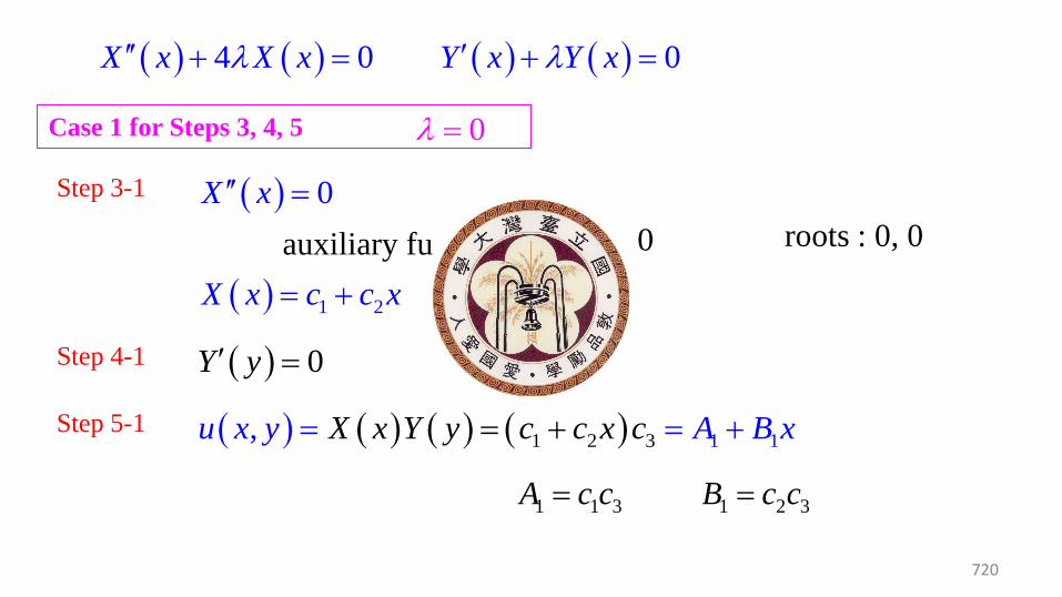
Step 3-1 ( ) 0X x′′ =

auxiliary function 2 0m =

Case 1 for Steps 3, 4, 5 0λ =

roots : 0, 0

( ) 1 2X x c c x= +

Step 4-1 ( ) 0Y y′ = ( ) 3Y y c=

( ) ( ) ( ) ( )2 11 13, X x Y y c c x cu x y A B x= += = +

1 1 3A c c= 1 2 3B c c=

Step 5-1

( ) ( )4 0X x X xλ′′ + = ( ) ( ) 0Y x Y xλ′ + =

720

Case 2 for Steps 3, 4, 5 0λ <為了方便起見，令 2λ α= −

( ) ( )24 0X x X xα′′ − =

( ) 2 21 2

x xX x d e d eα α−= +

通常將解改寫成 ( ) 4 5cosh(2 ) sinh(2 )X x c x c xα α= +

( )( )

2Y yY y

α′

=

roots of the auxiliary function: 2α, −2α

Step 4-2 ( ) ( )2 0Y y Y yα′ − =

( ) ( )2 0Y y Y yα′ − = ( )2

6yY y c eα=

( ) ( ) ( )2 2

2 2, cosh(2 ) sinh(2 )y yu x y A e xx eY y B xX α αα α= +=Step 5-2

2 4 6A c c= 2 5 6B c c=

Step 3-2

721

Case 3 for Step 3 0λ >為了方便起見，令 2λ α=

( ) ( )24 0X x X xα′′ + = roots of the auxiliary function: j2α, −j2α

( ) 7 8cos(2 ) sin(2 )X x c x c xα α= +

( )( )

2Y yY y

α′

= −Step 4-3 ( ) ( )2 0Y y Y yα′ + = ( )2

9yY y c e α−=

Step 5-3 ( )2 2

3 3, cos(2 ) sin(2 )y yu x y A e x B e xα αα α− −= +

若要處理 boundary conditions，將所有可能的解都加起來

( )2 2

2 2

1 1 2, 2,

3, 3,

, [ cosh(2 ) sinh(2 )]

[ cos(2 ) sin(2 )]

y y

y y

u x y A B x A e x B e x

A e x B e x

α αα α

α

α αα α

α

α α

α α− −

= + + +

+

∑

∑ α 是任意實數

Step 3-3

Step 6

722

12.1.4 Classification 2 2 2

2 2 0u u u u uA B C D E Fux y x yx y∂ ∂ ∂ ∂ ∂+ + + + + =

∂ ∂ ∂ ∂∂ ∂

2 4 0B AC− > The PDE is said to be hyperbolic (雙曲線)

2 4 0B AC− =

2 4 0B AC− <

The PDE is said to be parabolic (拋物線)

The PDE is said to be elliptic (橢圓形)

723

這些命名方式，是根據 2 次多項式在 x-y 平面上的軌跡 2 2 0Ax Bxy Cy Dx Ey F+ + + + + =2 2

2 2

1 01y

xx

y+

+ −

=

=當

2 4 4 0B AC− = − <

2

2 0yx

xy

=

=

−當

2 4 0B AC− =

x

y y

-3 -2 -1 0 1 2 3-3

-2

-1

0

1

2

3

-3 -2 -1 0 1 2 3-3

-2

-1

0

1

2

3

x 724

當 2 2

2 2

1 01y

xx

y−

− −

=

=

2 4 4 0B AC− = >

x

y

-3 -2 -1 0 1 2 3-3

-2

-1

0

1

2

3

記憶秘訣：只要清楚幾個「特例」，就可以記住當 2 4 0,B AC− < 2 4 0,B AC− = 2 4 0B AC− >

的時候，應該是什麼圖形 725

Example 2 (text page 435) 2

23 u uyx

∂ ∂=∂∂

2 2

2 2u u

x y∂ ∂=∂ ∂

2 2

2 2 0u ux y∂ ∂+ =∂ ∂

726

12.1.5 本節需要注意的地方

(1) 本節除了定義以外，只有兩個重點： classification of equations 以 及 method of separation of variables.

(2) 然而， method of separation of variables 解法的流程，稍有些複 雜，需要熟悉 (Sections 12-4, 12-5 都將用這個方法)

關鍵：記住第一步 u(x, y) = X(x)Y(y)

第二步 function of X = function of Y = −λ

(3) Method of separation of variables 在計算時，會分成很多個 cases.

(4) Separation of variables要解 BVP 和 IVP時，需要將每個 cases 得 出來的解都加起來 (Step 6)

727

2 21 2

x xd e d eα α−+

4 5cosh(2 ) sinh(2 )c x c xα α+

(5) 為了方便解決 BVP 或 IVP，經常將

改寫成

(6) Hyperbolic, parabolic, elliptic 的條件，可以用幾個 special

cases 來記

(7) “等於零” 的 BVP 或IVP 可以先於 Steps 3, 4 當中考慮

(例如 pages 742, 758 的下方)

“不等於零” 的 BVP 或IVP 則在 Step 7 當中處理

728

Section 12.2 Classical PDEs and Boundary- Value Problems 12.2.1 本節綱要

(1) one-dimensional heat equation (或簡稱為 heat equation) 2

2u uk tx

∂ ∂=∂∂

(2) one-dimensional wave equation (或簡稱為 wave equation)

k > 0

2 222 2u ua

x t∂ ∂=∂ ∂

(3) two-dimensional form of Laplace’s equation (或簡稱為 Laplace’s equation ) 2 2

2 2 0u ux y∂ ∂+ =∂ ∂ 729

名詞：

heat equation, (page 730) wave equation, (page 731)

Laplace’s equation, (page 734) Laplacian, (page 735)

Dirichlet condition, (page 738) Neumann condition, (page 738)

Robin condition (page 738)

本節的重點：熟悉這七大名詞，和它們所對應的公式

730

12.2.2 One-Dimensional Heat Equation

由來：熱傳導的理論 (推導過程見課本 438頁）

2

2u uk tx

∂ ∂=∂∂

heat equation 別名：diffusion equation

Fig. 12.2.1

u(x, t): temperature, t: time, x: location

731

12.2.3 One-Dimensional Wave Equation 2 22

2 2u ua

x t∂ ∂=∂ ∂

「拉像皮筋」的模型 (推導過程見課本 439頁）

u(x, t): height, t: time, x: location

(1) 開始 wave equation 別名： telegraph equation

732

Fig. 12.2.4

f(x)

(2) 手放開之後產生振動

Fig. 12.2.2

733

• Wave equation 其他的應用：

Theory of high-frequency transmission line

Fluid mechanics (流體力學)

Acoustics (聲學)

Elasticity (彈力學)

Microwave engineering (電波工程)

734

12.2.4 Two-Dimensional Form of Laplace’s Equation 2 2

2 2 0u ux y∂ ∂+ =∂ ∂

u(x, y): temperature,

x, y: location

如課本 Fig. 12.2.3，溫度隨著位置而變化的模型

735

Laplace’s Equation 亦可用 Laplacian 表示, ∇2u(x, y) = 0

Laplacian: ∇2

( )2 22

2 2, u uu x yx y∂ ∂∇ = +∂ ∂

( )2 2 22

2 2 2, , u u uu x y zx y z∂ ∂ ∂∇ = + +∂ ∂ ∂

736

• Laplace’s Equation 的其他應用

Static displacement of membranes

Edge detection (邊緣偵測)

Microwave engineering (電波工程)

737

12.2.5 Modification

( )2

2 mu uk h u u tx

∂ ∂− − =∂∂

加上外力，或與外界的交互作用

例：heat equation 的 modification

例：wave equation 的 modification

( )2 22

2 2, , , tu ua F x t u u

x t∂ ∂+ =∂ ∂

738

12.2.6 Boundary Conditions 或 Initial Conditions

Dirichlet condition

Neumann condition

u = …….. (沒微分)

un∂ =∂

Robin condition u hun∂ + =∂

(有微分)

(混合)

h is a constant

739

Section 12.4 Wave Equation 12.4.1 本節綱要

2 222 2u ua

x t∂ ∂=∂ ∂

要解決的問題 (one-dimensional wave equation)

0 < x < L

BVP and IVP ( )0, 0u t = ( ), 0u L t =

( ) ( ),0u x f x= ( )0t

u g xt =

∂ =∂

t > 0

for t > 0

for 0 < x < L

解法見 page 741-749 例子見 page 750 740

實際上，Sections 12.4 和 12.5 可看成是 Section 12.1 的 method of separation of variables 的練習題

(可見得 method of separation of variables 有多重要)

名詞：

standing waves (page 751) normal modes (page 751)

first standing wave (page 752) first normal mode (page 752)

fundamental frequency (page 752) nodes (page 754)

overtones (page 754)

741

12.4.2 Solutions for Wave Equations (自己挑戰解解看) 2 22

2 2u ua

x t∂ ∂=∂ ∂ 0 < x < L t > 0

四大條件 ( )0, 0u t =

( ) ( ),0u x f x=

( ), 0u L t =

( )0t

u g xt =

∂ =∂

for t > 0

for 0 < x < L

求解 (使用method of separation of variables)

Step 1 假設解為 u(x, t) = X(x)T(t)

Step 2

( ) ( ) ( ) ( )2a X x T t X x T t′′ ′′=

將 u(x, y) = X(x)T(t) 代入 2 22

2 2u ua

x t∂ ∂=∂ ∂

( )( )

( )( )2

X x T tX x a T t′′ ′′

=

742

令 ( )( )

( )( )2

X x T tX x a T t

λ′′ ′′

= = −

Steps 3, 4, 5 的前處理

(1) 因為 x 的 boundary condition 較簡單，所以先解 X(x)

( ) ( ) 0X x X xλ′′ + = ( ) ( )2 0T t a T tλ′′ + =得出2 個 ODEs

(2) 分成 λ = 0, λ < 0 , λ > 0 三個 cases

(3) 由於

( )0, 0u t = u(0, t) = X(0)T(t) = 0

所以 X(0) = 0

for all t > 0

同理，由 ( ), 0u L t = 可以立即判斷 X(L) = 0

T(t) 不可為 0 (否則 u(x, t) = X(x)T(t) = 0 for any x, t)

( ) ( ) 0X x X xλ′′ + = subject to X(0) = 0 and X(L) = 0

743

( ) ( ) 0X x X xλ′′ + =subject to X(0) = 0 and X(L) = 0

( ) ( )2 0T t a T tλ′′ + =

Case 1 for Steps 3, 4, 5 λ = 0

( ) 0X x′′ = ( ) 1 0X x d x d= +

根據 boundary conditions

0 0d =1 0 0d L d+ =

0 0d =

1 0d = ( ) 0X x =

這個 case 得出 trivial solution u(x, t) = X(x)T(t) = 0

將無法滿足 ( ) ( ),0u x f x= λ = 0 時無解

Step 3-1

無需再解 Step 4-1, Step 5-1 744

Case 2 of Steps 3, 4, 5: λ < 0

令 λ = −α2

( ) ( )2 0X x X xα′′ − =

Solution: ( ) 2 3x xX x d e d eα α−= +

可改寫成 ( ) ( ) ( )4 5cosh sinhX x d x d xα α= +

根據 boundary conditions X(0) = 0 and X(L) = 0

4 0d =( ) ( )4 5cosh sinh 0d L d Lα α+ =

4 0d =

5 0d =( ) 0X x =

這個 case 得出 trivial solution u(x, t) = X(x)T(t) = 0

將無法滿足 ( ) ( ),0u x f x= λ < 0 時無解

Step 3-2

無需再解 Step 4-2, Step 5-2 745

Case 3 of Steps 3, 4, 5: λ > 0

令 λ = α2

( ) ( )2 0X x X xα′′ + =

( ) 1 2cos sinX x c x c xα α= +Solution: 根據 boundary conditions X(0) = 0 and X(L) = 0

1 0c =1 2cos sin 0c L c Lα α+ =

1 0c =nLπα =

2c = any nonzero constant

特別注意：

不可直接由 就斷言

應該看看是否有適當的 α, 讓第二個式子等於零

1

1 2

0cos sin 0

cc L c Lα α=

+ =

n 是任意整數

Step 3-3

1

2

00

cc=

=

746

( ) 2 sin nX x c xLπ=

nLπα =

2 222

nLπλ α= =

Step 4-3 ( ) ( )2 0T t a T tλ′′ + =

( ) ( )2 2 2

2 0a nT t T tLπ′′ + =

Solution: ( ) ( ) ( )3 4cos sinna naT t c t c tL Lπ π= +

Step 5-3 ( ) ( ) ( ) ( ) ( ) ( )( ) ( ) ( )

2 3 4sin,

sin cos

cos

n

s

i

in

s

n

n n

n na nac x c t c tL L Lu x t X x T t

n na nax A t B tL L Lπ π

π

π

π π= =

= +

+

n 是任意整數

n 是任意整數

An = c2c3, Bn = c2c4, 747

注意： ( ) ( ) ( ) ( ), sin cos sinn n nn na nau x t x A t B tL L Lπ π π = +

只是其中一個解，因為 n 是任意整數

( ) ( ) ( ) ( ) ( )1 1

, sin co, s sinnnn

n nn na nau x t x A t B tL L Lu x t π π π

∞ ∞

= =

= = + ∑ ∑

Step 6

748

討論：既然 n 是任意整數，那為什麼 n 是從1 加到 ∞，

而非由 − ∞ 加到 ∞ ？

( ) ( ) ( )( ) ( ) ( )

1

sin cos sin

sin cos sin

n nn

n nn

n na nax C t D tL L L

n na nax A t B tL L L

π π π

π π π

∞

=−∞

∞

=

+

= +

∑

∑

因為

( ) ( )sin sin ,na nat tL Lπ π−= −

( ) ( )cos cos ,na nat tL Lπ π−=

( )sin 0 0=

n n nA C C−= +

可證明

n n nB D D−= −

( ) ( )sin sin ,n nx xL Lπ π−= −

749

Step 7

由 initial conditions

( ) ( ) ( ) ( )1

, sin cos sinn nn

n na nau x t x A t B tL L Lπ π π

∞

=

= + ∑

( ) ( ),0u x f x= ( )0t

u g xt =

∂ =∂

( ) ( )1

sinnn

nf x A xLπ

∞

=

=∑ ( ) ( )1

sinnn

na ng x B xL Lπ π

∞

=

=∑

也就是說，An 是 f(x) 的 Fourier sine series,

是 g(x) 的 Fourier sine series nnaB Lπ

( )0

2 sinL

nnA f x xdxL Lπ= ∫

( )0

2 sinL

nna nB g x xdxL L Lπ π= ∫ ( )

02 sin

L

nnB g x xdxna Lπ

π= ∫750

2 222 2u ua

x t∂ ∂=∂ ∂

( )0, 0u t = ( ), 0u L t =

( ) ( ),0u x f x= ( )0t

u g xt =

∂ =∂

12.4.3 物理意義

ut

∂∂ : 速度

2

2u

t∂∂

: 加速度

u : 高度

Fig. 12.2.4

f(x)

751

12.4.4 名詞

( ) ( ) ( ) ( )1

, sin cos sinn nn

n na nau x t x A t B tL L Lπ π π

∞

=

= + ∑

( ) ( ) ( ) ( )1 2 3, , , ,u x t u x t u x t u x t= + + +

( ) ( ) ( ) ( )( ) ( )

, sin cos sin

sin sin

n n n

n n

n na nau x t x A t B tL L Ln naC x tL L

π π π

π π φ

= +

= +

un(x, t) 被稱作 standing waves (駐波) 或 normal modes

2 2n n nC A B= + cos n

nn

BCφ = sin n

nn

ACφ =

其中

752

n = 1 時， u1(x, t) 被稱作 first standing wave 或 first normal mode 或 fundamental mode of vibration

( ) ( ) ( )1 1 1, sin sin au x t C x tL Lπ π φ = +

( ) ( ) ( ) ( )1 1 1 12, sin sin 2 ,aLu x t C x t u x ta L L

π π π φ + = + + =

對於 t 而言，週期 = 2La

頻率 =1/週期 2aL=

1 2af L= 被稱作 fundamental frequency (基頻) 或 first harmonic

753

以此類推， u2(x, t) 被稱作 second standing wave u3(x, t) 被稱作 third standing wave

Fig. 12.*.*

First standing wave

Second standing wave

Third standing wave

754

( ) ( ) ( ), sin sinn n nn nau x t C x tL Lπ π φ = +

Lx n= 時，無論 t 等於多少， ( ), 0nLu tn =

Lx n= 是 nth standing wave 的 node (節點)

( ) ( )2, ,n nLu x t u x t an= +

un(x, t) 的頻率 =1/週期 = 2an L

12naf n nfL= = 被稱作 overtones (泛音)

755

Section 12.5 Laplace’s Equation 12.5.1 Section 12.5 綱要

2 2

2 2 0u ux y∂ ∂+ =∂ ∂

0 < x < a, 0 < y < b,

00

x

ux =

∂ =∂

0x a

ux =

∂ =∂

for 0 < y < b,

( ),0 0u x = ( ) ( ),u x b f x= for 0 < x < a

(使用method of separation of variables 來解)

「問題 1」

「問題 2」 ( )0, 0u y = ( ), 0u a y =

( ),0 0u x = ( ) ( ),u x b f x= for 0 < x < a for 0 < y < b,

「問題 3」 ( ) ( )0,u y F y= ( ) ( ),u a y G y=( ) ( ),0u x f x= ( ) ( ),u x b g x=

for 0 < x < a for 0 < y < b,

756

※ 注意 “superposition principle”

(唯一真正的新東西)

Sections 12.4, 12.5 的重點，大致歸於二類

(1) Method of separation of variables 的練習

(2) Superposition principle

PS: 如果各位的記憶力真的遠超過於常人，想要把 wave equations

和 Laplace’s equations 的 solutions 背起來，我也不反對啦！

757

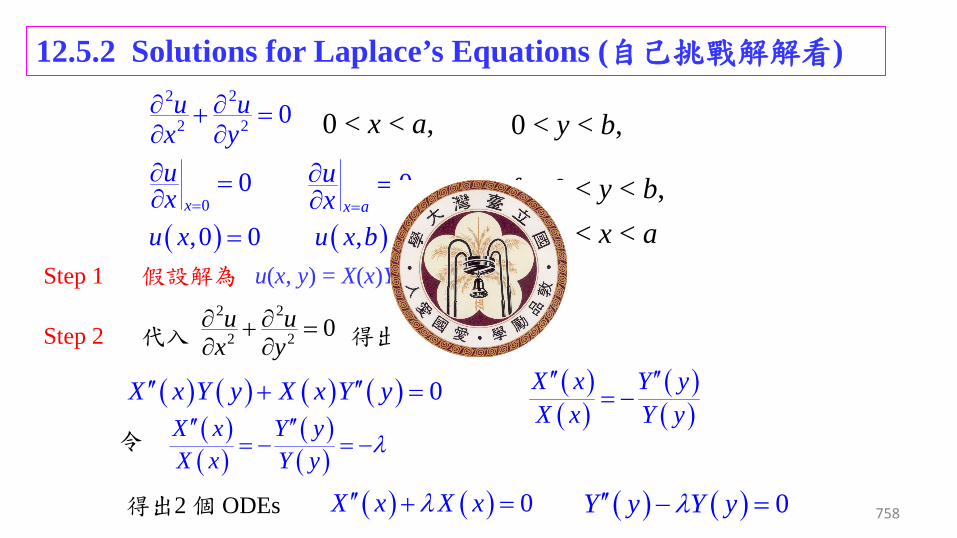
12.5.2 Solutions for Laplace’s Equations (自己挑戰解解看) 2 2

2 2 0u ux y∂ ∂+ =∂ ∂ 0 < x < a, 0 < y < b,

00

x

ux =

∂ =∂ 0

x a

ux =

∂ =∂ for 0 < y < b,

( ),0 0u x = ( ) ( ),u x b f x= for 0 < x < a Step 1 假設解為 u(x, y) = X(x)Y(y)

Step 2 代入 得出 2 2

2 2 0u ux y∂ ∂+ =∂ ∂

( ) ( ) ( ) ( ) 0X x Y y X x Y y′′ ′′+ = ( )( )

( )( )

X x Y yX x Y y′′ ′′

= −( )( )

( )( )

X x Y yX x Y y

λ′′ ′′

= − = −令

( ) ( ) 0X x X xλ′′ + = ( ) ( ) 0Y y Y yλ′′ − =得出2 個 ODEs 758

Steps 3, 4, 5 的前處理

(1) 因為 x 的 boundary condition 較簡單，所以先解 X(x)

(2) 分成 λ = 0, λ < 0 , λ > 0 三個 cases

(3) 由於

( ) ( ) ( ) ( )0

0 0x

X x Y yX Y yx

=

∂ ′= =∂

for all 0 < y < b,

Y(y) 不可為 0 (否則 u(x, y) = X(x)Y(y) = 0)

所以 ( )0 0X ′ =

同理，由 ( ) 0X a′ =0x a

ux =

∂ =∂

00

x

ux =

∂ =∂

同理，由 ( ),0 0u x = ( )0 0Y =759

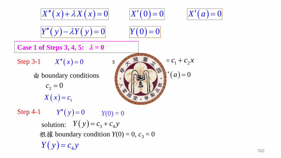
Step 3-1

( ) ( ) 0X x X xλ′′ + = ( )0 0X ′ = ( ) 0X a′ =

( ) ( ) 0Y y Y yλ′′ − =

Case 1 of Steps 3, 4, 5: λ = 0

( ) 0X x′′ = solution: ( ) 1 2X x c c x= +

由 boundary conditions ( )0 0X ′ = ( ) 0X a′ =

2 0c =

( ) 1X x c=

Step 4-1

solution:

( ) 0Y y′′ = Y(0) = 0 ( ) 3 4Y y c c y= +

( ) 4Y y c y=

( )0 0Y =

根據 boundary condition Y(0) = 0, c3 = 0

760

( ) ( ) ( ) 1 04, X x Y yu Ac ycy yx == = 0 1 4A c c=Step 5-1

Case 2 of Steps 3, 4, 5: λ < 0

令 λ = −α2

Step 3-2 ( ) ( )2 0X x X xα′′ − = ( )0 0X ′ = ( ) 0X a′ =

solution: ( ) 2 3x xX x d e d eα α−= +

( ) ( ) ( )4 5cosh sinhX x d x d xα α= +可改寫成

由 boundary conditions ( )0 0X ′ = ( ) 0X a′ =

( ) ( )cosh sinh ,d x xdx α α α= ( ) ( )sinh coshd x xdx α α α=以及

5 0d α =

( ) ( )4 5sinh cosh 0d a d aα α α α+ =5 0d =4 0d = ( ) 0X x =

761

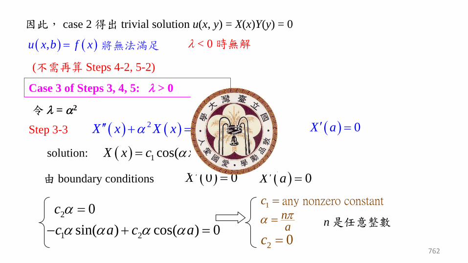
因此， case 2 得出 trivial solution u(x, y) = X(x)Y(y) = 0

將無法滿足 ( ) ( ),u x b f x= λ < 0 時無解

(不需再算 Steps 4-2, 5-2)

Case 3 of Steps 3, 4, 5: λ > 0

令 λ = α2

Step 3-3 ( ) ( )2 0X x X xα′′ + = ( )0 0X ′ = ( ) 0X a′ =

solution: ( ) 1 2cos( ) sin( )X x c x c xα α= +

由 boundary conditions ( )0 0X ′ = ( ) 0X a′ =

2 0c α =

1 2sin( ) cos( ) 0c a c aα α α α− + =2 0c =

naπα =

1c = any nonzero constant

n 是任意整數

762

再次注意：不可直接判斷成 c1 = 0 and c2 = 0

應該看看是否有適當的 α, 讓第二個式子等於零

( ) 1 cosnnX x c xaπ= n 是任意整數

2 222

naπλ α= =

Step 4-3 ( ) ( )2 2

2 0nY y Y yaπ′′ − =

Y(0) = 0

( ) ( ) ( )3 4cosh sinhnn nY y c y c ya aπ π= +經常改寫為

solution:

根據 boundary condition Y(0) = 0 3 0c =

( ) ( )4 sinhnnY y c yaπ=

( ) 3 4

n ny ya anY y d e d e

π π−= +

since 2 2

2naπλ =

763

( ) ( ) ( ) ( ) ( ) ( ) ( )1 4cos sin, cos si hh nnn nX x Y y c x c ya a

n nu x y A x ya aπ ππ π== =

1 4nA c c=

Step 5-3

Step 6 把所有可能的解，全部加起來

( ) ( ) ( )01

, cos sinhnn

n nu x y A y A x ya aπ π

∞

=

= +∑

為什麼 n 是從 1 加到 ∞，而非由 −∞ 加到 ∞？

道理同講義 page 748

n 是任意整數

764

Step 7 ( ) ( ) ( )01

, cos sinhnn

n nu x y A y A x ya aπ π

∞

=

= +∑

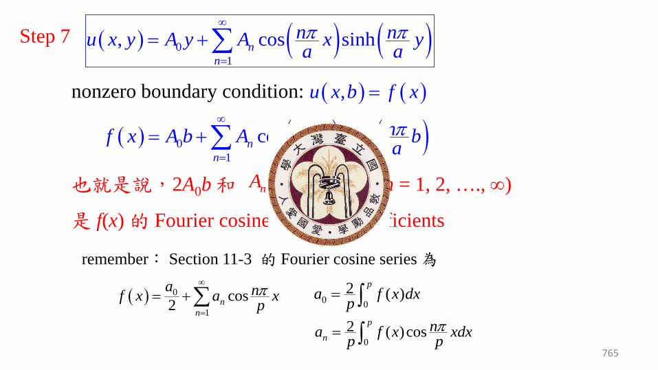
( ) ( ),u x b f x=nonzero boundary condition:

( ) ( ) ( )01

cos sinhnn

n nf x A b A x ba aπ π

∞

=

= +∑也就是說，2A0b 和 (n = 1, 2, …., ∞)

是 f(x) 的 Fourier cosine series 的 coefficients

( )sinhnnA baπ

( ) 0

1cos2 n

n

a nf x a xpπ

∞

=

= +∑

remember： Section 11-3 的 Fourier cosine series 為

0 02 ( )

pa f x dxp= ∫

02 ( )cos

p

nna f x xdxp pπ= ∫

765

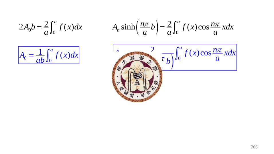
0 022 ( )

aA b f x dxa= ∫ ( ) 0

2sinh ( )cosa

nn nA b f x xdxa a aπ π= ∫

0 01 ( )

aA f x dxab= ∫ ( ) 0

2 ( )cossinh

a

nnA f x xdxana ba

ππ

= ∫

766

12.5.3 Laplace’s Equations with Dirichlet Problem 2 2

2 2 0u ux y∂ ∂+ =∂ ∂

0 < x < a, 0 < y < b,

( )0, 0u y = ( ), 0u a y =

( ),0 0u x = ( ) ( ),u x b f x=

0 < y < b,

0 < x < a,

用 method of separation of variables，經過計算得出

( )1

, sinh sinnn

n nu x y A y xa aπ π

∞

=

=∑

( )0

2 sinsinh

a

nnA f x xdxn aa ba

ππ= ∫ 可自行練習解解看

767

12.5.4 Superposition Principle

Dirichlet Problem 可分解成兩個子問題

2 2

2 2 0u ux y∂ ∂+ =∂ ∂ 0 < x < a, 0 < y < b,

( ) ( )0,u y F y= ( ) ( ),u a y G y= for 0 < y < b,

( ) ( ),0u x f x= ( ) ( ),u x b g x= for 0 < x < a,

當四個邊界都不為零時，很難直接用 separation of variable 的方法

解出來

768

子問題 1 2 2

2 2 0u ux y∂ ∂+ =∂ ∂ 0 < x < a, 0 < y < b, ( )0, 0u y = ( ), 0u a y =( ) ( ),0u x f x= ( ) ( ),u x b g x=

for 0 < y < b, for 0 < x < a,

子問題 2 2 2

2 2 0u ux y∂ ∂+ =∂ ∂

0 < x < a, 0 < y < b,

( ) ( )0,u y F y= ( ) ( ),u a y G y= for 0 < y < b, ( ),0 0u x = ( ), 0u x b = for 0 < x < a,

假設 u1(x, y), u2(x, y) 分別是子問題 1, 子問題 2 的解

則 u (x, y) = u1(x, y) + u2(x, y) 是原來問題的解

(類似於 Section 4-1 的 superposition principle) 769

770

u (0, y) = u1(0, y) + u2(0, y) = 0 + F(y) = F(y)

當 u (x, y) = u1(x, y) + u2(x, y)

u (a, y) = u1(a, y) + u2(a, y) = 0 + G(y) = G(y)

u (x, 0) = u1(x, 0) + u2(x, 0) = f(x) + 0 = f(x)

u (x, b) = u1(x, b) + u2(x, b) = g(x) + 0 = g(x)

= +

子問題 1 的解 ( ) { }11

, cosh sinh sinn nn

n n nu x y A y B y xa a aπ π π

∞

=

= +∑

( ) ( )02 sin

a

nnA f x x dxa aπ= ∫

( ) ( ) ( ) ( )01 2 sin cosh

sinh

a

n nn nB g x x dx A ba a an ba

π ππ

= − ∫

子問題 2 的解 ( ) { }21

, cosh sinh sinn nn

n n nu x y A y B y xb b bπ π π

∞

=

= +∑

( ) ( )02 sin

b

nnA F y y dyb bπ= ∫

( ) ( ) ( ) ( )01 2 sin cosh

sinh

b

n nn nB g x x dx A ab b bn ab

π ππ

= − ∫

原來問題的解 ( ) ( )1 2, ,u x y u x y+771

12.5.5 Sections 12.4 及 12.5 需要注意的地方

(1) Method of separation of variables 解 PDE 的過程雖然長，但是把握住講義 pages 713-715 的 7 個 steps，並練習幾次，就可以熟悉。

(這些對大二下和大三上的電磁學很重要)

(2) 雖然概念不難，但是計算過程很長且繁雜

所以一定要多研究簡化運算、快速判斷的方法

772

(3) 有沒有注意到，

若 boundary conditions 出現 u(0, y) = 0, u(L, y) = 0,

最後的解總是和 sine 有關

若 boundary conditions 出現

最後的解總是和 cosine 或 constant 有關 0

0x

ux =

∂ =∂ 0

x L

ux =

∂ =∂

( ) 2 sin nX x c xLπ= 週期為 2L/n

( ) 1 cosnnX x c xLπ=( ) 1X x c= or 週期也為 2L/n

(4) 經驗足夠後，看到 u(x, y) 的 boundary conditions

出現 u(a, y) = 0 就知道 X(a) = 0 ，

看到 u(x, b) = 0 就知道 Y(b) = 0 。

看到 就知道 X'(a) = 0，

看到 就知道 Y'(b) = 0

0x a

ux =

∂ =∂

0y b

uy =

∂ =∂ 773

(5) 對於 wave equations 而言， X(x) 和 T(t) 的解有相同的型態

如果 X(x) 為 sine & cosine, T(t) 也為 sine & cosine

對於 Laplace’s equations而言， X(x) 和 Y(y) 的解型態不同

如果X(x) 為 sine & cosine, Y(y) 為 sinh & cosh

( )( )

( )( )2

X x T tX x a T t

λ′′ ′′

= = − ( )( )

( )( )

X x Y yX x Y y

λ′′ ′′

= − = −

2 2

2 2 0u ux y∂ ∂+ =∂ ∂

2 222 2u ua

x t∂ ∂=∂ ∂

(6) 要熟悉 cosh(x), sinh(x) 的性質 774

(7) Method of separation of variables 在計算上容易出錯的地方

(以 講義 pages 741-749 wave equations 為例)

(a)

(b) Steps 3, 4, 5 要考慮所有 cases

(c) 不可直接由 c1 = 0 及 判斷 c1 = c2 = 0

因為 α 可以是 πn/L, 如講義 page 745 所述

(d) 在 Step 6，要將所有可能的解加起來，才是 u(x, t) 的一般解

( )( )

( )( )2

X x T tX x a T t

λ′′ ′′

= −=

1 2cos sin 0c L c Lα α+ =

775

Section 12-1 2, 3, 6, 9, 12, 16, 18, 22, 23, 27, 30

Section 12-2 3, 4, 8, 9

Section 12-4 1, 3, 4, 7, 8, 9, 11, 14

Section 12-5 2, 5, 6, 9, 11, 12, 14, 16, 17, 18

Review 12 1, 2, 6

Exercise for Practice

776

祝各位期末考順利，寒假愉快！

Happy New Year!

777

版權聲明

頁碼 作品 版權標示 作者/來源

723 國立臺灣大學 電信工程所 丁建均 教授

723 國立臺灣大學 電信工程所 丁建均 教授

724 國立臺灣大學 電信工程所 丁建均 教授

730 國立臺灣大學 電信工程所 丁建均 教授

778

-3 -2 -1 0 1 2 3-3

-2

-1

0

1

2

3

-3 -2 -1 0 1 2 3-3

-2

-1

0

1

2

3

-3 -2 -1 0 1 2 3-3

-2

-1

0

1

2

3

版權聲明

頁碼 作品 版權標示 作者/來源

731 國立臺灣大學 電信工程所 丁建均 教授

732 國立臺灣大學 電信工程所 丁建均 教授

753 國立臺灣大學 電信工程所 丁建均 教授

753 國立臺灣大學 電信工程所 丁建均 教授

779

版權聲明

頁碼 作品 版權標示 作者/來源

756 國立臺灣大學 電信工程所 丁建均 教授

756 國立臺灣大學 電信工程所 丁建均 教授

756 國立臺灣大學 電信工程所 丁建均 教授

780