Differentiable (analytical, or smooth) functions: ( )

SHAPE ANALYSIS AND CLASSIFICATION30

A function where both U and W are real subsets (i.e., RWU ⊂, ) is called areal function. Examples of real functions include:

Figure 2.1: Graphical representations of some types of functions (see text forexplanation)

( ) 2|: xxfyRRf ==→

and

( )otherwise

wRwwtifttgyRRg

0,,0

0|:

>∈≤≤

==→

The visual representation of real functions is always useful as a means tobetter understand their characteristics. Figure 2.2 depicts the graphicalrepresentations of the aforementioned functions.

Some special types of functions include:

Differentiable (analytical, or smooth) functions: These are functions for

which all derivatives exist. For instance, the function ( ) 2ttf = is

differentiable in R, and its first derivative is ( ) tdt

dftf 2' == . In case the

derivatives exist only up to a maximum order k , the function is said to be

Mathematical Concepts 49

angle y with the real axis. Observe that this ray does not reach the planeorigin. The above mapping can be graphically represented as in Figure 2.27.

j j

exp{a}

c

a

c

Figure 2.27: The mapping of vertical and horizontal lines by ( ) ( )zzg exp= .

Now, consider the rectangular region of the domain space defined as

bxa ≤≤ and dyc ≤≤

The reader should have no difficulty verifing that this rectangular region ismapped by g(z) as illustrated in Figure 2.28.

j j

c

a

d

b

g(z)

Figure 2.28: The mapping of a rectangle by ( ) ( )zzg exp= .

Figure 2.29 presents a more comprehensive illustration of the mappingimplemented by ( ) ( )zzg exp= with respect to an orthogonal grid in the

domain space.As is clear from the above example, it is not always easy to identify the

more interesting behavior to be illustrated for each specifically consideredcomplex function.


A non-empty subset X of a vector space S, such as the addition betweenany of its elements and the product of any of its elements by a scalar result avector in X (i.e., closure with respect to addition and multiplication by a scalar),

is called a subspace of S . It can be readily verified that the null vector 0r

mustbe included in any subspace. For instance, the space R is a subspace of R2. Inaddition, observe that a subspace is also a vector space.

Given M vectors ipr

; i = 1, 2, … , M; in the vector space S, the linear

combination of such vectors, resulting a vector qr

also in S, is defined as

MM papapaqr

Lrrr

+++= 2211

where ai are any scalar values. The above M vectors are said to be linearlyindependent (l.i.) if and only

0

0

21

2211

===⇔⇔++++=

M

MMii

aaa

papapapa

L

rL

rL

rrr

In other words, it is not possible to express one of the vectors as a linearcombination of the other vectors. Otherwise, the M vectors are said to belinearly dependent (l.d.). A practical way to determine whether a set ofvectors is l.i. can be obtained by using the determinants or rank of matrices, asdescribed in Sections 2.2.5.3 and 2.2.5.6, respectively.

For any vector space S, it is always possible to identify a minimal set, in thesense of involving the minimum number of elements, of linearly independentvectors in S whose linear combinations produce (or span) all the possiblevectors in S. Such a set of elementary vectors is called a basis of S. Forinstance, both

=

0

1,

1

01B and

−

=1

1,

1

02B

are valid bases for R2. The dimension of a vector space is defined as thenumber of vectors in any of the bases spanning this space. It should beobserved that the vector space containing only the null vector has dimensionzero and not one. The above examples (vii) and (viii) of vector spaces haveinfinite dimension.

Let S be an N-dimensional vector space and { }NbbbBr

Lrr

,,, 21= be one

of its possible bases. Then any vector pr

in this space can be represented as

a unique linear combination of the vectors in B, i.e.,

NN bababapr

Lrrr

+++= 2211 , and scalars Naaa ,,, 21 L are called


coordinates of the vector pr

with respect to basis B, which are often

represented as

[ ]TBN

BN

aaa

a

a

a

p LM

r21

2

1

=

=

Although a vector space can have an infinite number of alternative bases,it always has a special basis, in the sense of being the most elementary andsimple one, which is called its respective canonical basis. For instance, thespace RN has the following canonical basis:

{ }

==

1

0

0

;;

0

1

0

;

0

0

1

,,, 21M

LMM

rL

rrNN eeeC

These are the bases normally adopted as default for representing vectors.In such situations, the subscript indicating the basis is often ommited. Forinstance:

+

+

−=

−=

−

1

0

0

2

0

1

0

3

0

0

1

1

2

3

1

2

3

1

3C

It makes no sense to think about the orientations of these vectors withrespect to some absolute reference, since this is not known to exist in theuniverse. What does matter are the intrinsical properties of the canonicalbasis, such as having unit magnitude and being orthogonal (see Section 2.2.4).Observe that all the thus far presented examples in this chapter haveconsidered canonical bases.

Now, let vr

be a vector originally represented in terms of its coordinateswith respect to the basis { }NaaaA

rL

rr,,, 21= . What will the new coordinates

of this vector be when it is expressed with respect to the new basis

{ }NbbbBr

Lrr

,,, 21= ? This important problem, known as change of

coordinates, can be addressed as follows. We start by expressing the vectorsin the new basis B in terms of the coordinates relative to the original basis A:

NN aaabr

Lrrr

1,21,211,11 ααα +++=


BA

NNNNN

N

N

N

A vCv

v

v

v

v

v

v

vrr

L

L

LLL

L

L

L

r=⇔

=

= 2

1

,2,1,

,22,21,2

,12,11,1

2

1

ˆ

ˆ

ˆ

ααα

αααααα

(2.9)

Now, provided C is invertible (see Section 2.2.5.8), we have

AB vCvrr 1−= (2.10)

which provides a practical method for changing coordinates. The aboveprocedure is illustrated in the accompanying box.

Example: Change of Coordinates

Find the coordinates of the vector ( )TAv 2,1−=r

(represented with respect to

the canonical basis) in the new basis defined by

( ) ( ){ }TT bbB 0,2;1,1 21 −===rr

.

Solution:

Since matrix C is readily obtained as

−=

01

21C , we have

=

−

−

== −

5.1

2

2

1

5.05.0

101AB vCv

rr

Figure 2.32 shows the representation of the above vector with respect toboth considered bases.

Figure 2.32: The vector vr

represented with respect to both considered bases.The axes defined by bases A and B are represented by thin and thick arrows,

respectively.


Linear transforms taking vectors from an N-dimensional space into an M-dimensional space, M<N, (i.e., transformations which are not full rank) are saidto be degenerated, and to find its inverse in this case is impossible. It shouldbe observed at this early stage of the book that this type of transformationcharacterizes a large number of practical situations in shape analysis andvision. For instance, the 2D projections of the 3D world falling onto ourretinas (or onto a digital camera) provide but a degenerate representation ofthe 3D imaged objects.

An important class of linear transformation is that implementing rotations.Figure 2.33 illustrates such a situation with respect to a vector v

r in the plane

pointing at a point P, where the new and old coordinate systems arerepresented by full and dotted axes, respectively. It should be observed thatrotating the old system by an angle θ (counterclockwise, with respect to the x-axis) corresponds to rotating vector v

r, with respect to the coordinate system,

by an angle –θ. Consequently, both these problems can be treated in the sameunified way.

The matrix representing the linear transformation, which rotates thecoordinate system of the two-dimensional space R2 by an angle θcounterclockwise, is immediately obtained by using the coordinates exchangeprocedure discussed in Section 2.2.2. We start by expressing the basis vectors

of the new space, i.e., { }jiB ~,~~ = , in terms of the vectors of the old basis

{ }jiB ˆ,̂ˆ = :

Figure 2.33: Rotations of the coordinate system can be implemented by a specificclass of linear transformations.

( ) ( ) jii ˆsinˆcos~ θθ +=


It is easy to see that a space allowing an inner product is also a normed andmetric space, since we can always define a norm in terms of the inner product

by making ppprrr

,+= .

Although not every vector space is normed, metric or allows innerproducts, most developments in the present book deal with concepts relatedto vector spaces with inner products. The box Metrics in CN exemplifies someof the valid norms, distances and inner products in those spaces.

Example: Metrics in CN

Let ( )TNpppp ,,, 21 L

r= and ( )T

Nqqqq ,,, 21 Lr

= be two generic vectors in

the N-dimensional complex space CN.

Norms of pr

:

Euclidean: 222

212 Npppp +++= L

r

City-block : Npppp +++= Lr

211

Chessboard : { }NpppMaxp ,,, 21 Lr

=∞

Distances between pr

and qr

:

Euclidean:

( ) ( ) ( )2222

2112 NN qpqpqpqp −++−+−=− L

rr

City-block :

NN qpqpqpqp −++−+−=− Lrr

22111

Chessboard : { }NN qpqpqpMaxqp −−−=−

∞,,, 2211 L

rr

Inner product between pr

and qr

:

( ) NNT qpqpqpqpqpqp *

2*21

*1

*., L

rrrrrr++===

Example: Norms, Distances and Inner Products in Function Spaces

Let f(t) and g(t) be two generic functions in the space of the continuousfunctions in the interval [a, b], i.e., C[a, b].

Norm of f(t):


[ ]

=⇒

N

iNiiiiii

p

p

p

p

aaaaq

M

MLL

2

1

,,2,1,

Consequently, the elements of the vector resulting from a lineartransformation can be understood as a measure of similarity between theorientations of the input vector p

r and each of the respective vectors defined

by the rows of the transformation matrix. This interpretation is essential forthe full conceptual understanding of several properties in signal and imagetransforms, including the Fourier and Karhunen-Loève transforms.

2.2.5 More about Vectors and MatricesWe have thus far limited our discussion of vectors and matrices as elements ofvector spaces, and as representations of linear transforms. This sectionprovides additional concepts and properties including the more general casesof complex vectors and matrices, i.e., those vectors and matrices havingcomplex numbers as elements, such as

+−

=

3

1

2

j

jvr

+−−−=

220

13

301

j

jj

j

A

2.2.5.1 Some Basic ConceptsThe null N×N matrix, henceforth represented as Φ, is a matrix having allelements equal to zero. A matrix A having dimension N×N is said to be asquare matrix. Its main diagonal corresponds to the elements ai,i, i = 1, 2, …,N. A square matrix having all the elements below (above) its main diagonalequal to zero is said to be an upper (lower) triangular matrix, as illustrated inthe following:

+−=

500

130

209

j

j

A is upper triangular,

and


−+=

542

0230

009

j

jB is lower triangular.

The identity matrix, represented as I, is a square matrix having ones alongits main diagonal and zeroes elsewhere. For example, the 3×3 identity matrix is

=

100

010

001

I

The complex conjugate of a matrix (vector) is obtained by taking thecomplex conjugate of each of its elements. For instance, the complexconjugate of the above matrix B is

+−=

542

0230

009*

j

jB

The derivative of a matrix is given by the derivatives of each of itscomponents. For instance

If

( )( )

−−+

+=

2

3

232

2sin

2cos31

tjt

ttj

tjtt

A

π,

then

( ) ( )( )

−

−+=

t

t

tjjt

dt

dA

202

12cos20

2sin2190 2 ππ

Given an N×M matrix A and an M×N matrix B, the product between A andB, indicated as C = AB, is defined as

∑=

=M

kjkkiji bac

1,,, (2.11)


-4 -3 -2 -1 0 1 2 3 4-80

-60

-40

-20

0

2 0

4 0

6 0

8 0

1 0 0

1 2 0

x

y

Figure 2.39: The original points (squares) and the obtained cubic polynomial.

The procedure illustrated in the above example can be generalized to anypolynomial or function. As a matter of fact, in the particular case of straightline fitting, we have the general line equation:

xaay 10 +=

and, therefore:

=

Nx

x

x

C

1

1

1

2

1

MM;

=

Ny

y

y

bM

r2

1

; and

=

1

0

a

axr

Applying Equation (2.15):

( ) =

⇒=

1

02

1

21

1

1

1

111

a

a

x

x

x

xxxbCxCC

N

N

TT

MML

Lrr


−

−

=

−

⇔Λ=

40

02

13

31

ba

ba

ba

baVAV

Designing Matrices to Have Specific Eigenvectors: Section 2.2.5.9 has brieflyaddressed the situation where we wanted to identify the eigenvalues andeigenvectors of a specific square matrix A. Here we present how to build amatrix A having a specific N×1 eigenvector v

r or a set of Nk ≤ orthogonal

eigenvectors ivr

with dimension N×1. In the former case, the sought matrix

is TvvArr

= , since:

( ) ( ) RvvrvrvvvvvvvAvvA TTTT ∈====⇒=rrrrrrrrrrrr

,

Observe that the matrix product Tvvrr

can be understood in terms of theabove concept of building a matrix by columns. This product implies thatvector v

r is copied into a subsequent column j of A weighted by each of its

respective coordinates vj. This implies that matrix A columns are all equalexcept for a multiplicative constant, and therefore A necessarily has rank 1.

In the latter case, i.e., we want Nk ≤ orthogonal eigenvectors ivr

; i = 1, 2,

…, k ; the matrix A is also easily obtained as

( )( ) Rvvrvrvvv

vvvvvvvvAvvvvvvA

iT

iiiT

ii

iTkk

TTi

Tkk

TT

∈===

=+++=⇒+++=rrrrrr

rrrL

rrrrrrrL

rrrr

,

22112211

It can be verified that the so obtained matrix A has rank k .

To probe further: Functions, Matrices and Linear Algebra

A good and relatively comprehensive introduction to many of the coveredissues, including propositional logic, functions, linear algebra, matrices,calculus and complex numbers can be found in [James, 1996]. A moreadvanced reference on mathematical concepts include the outstandingtextbook by [Kreyszig, 1993], which covers linear algebra, calculus, complexnumbers, and much more. Other good general references are [Bell, 1990] and[Ma Fong 1997]. Interesting references covering complementary aspectsrelated to mathematical physics, including variational calculus, are provided by[Boas, 1996] and [Dettman, 1988]. For those interested in probing further intofunction vector spaces (i.e., functional analysis), the books [Oden, 1979;Halmos, 1958; Michel and Herget, 1981; Kreyszig, 1993] provide excellentreading, also including good reviews of basic concepts. An interestingapproach to complex number and analysis, based on visualization of the


( ) ( )( )tp

tptn

&&r

&&rr=

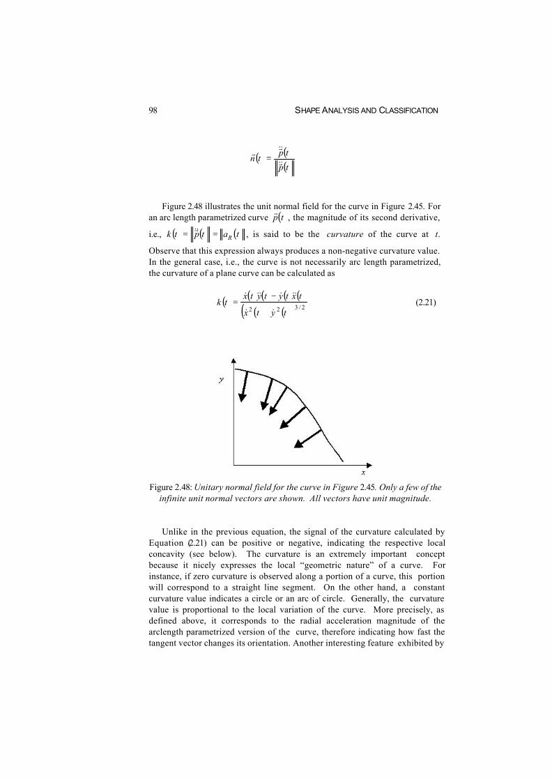
Figure 2.48 illustrates the unit normal field for the curve in Figure 2.45. Foran arc length parametrized curve ( )tp

r, the magnitude of its second derivative,

i.e., ( ) ( ) ( )tatptk R== &&r , is said to be the curvature of the curve at t.

Observe that this expression always produces a non-negative curvature value.In the general case, i.e., the curve is not necessarily arc length parametrized,the curvature of a plane curve can be calculated as

( ) ( ) ( ) ( ) ( )( ) ( )( ) 2/322 tytx

txtytytxtk

&&

&&&&&&

+

−= (2.21)

Figure 2.48: Unitary normal field for the curve in Figure 2.45. Only a few of theinfinite unit normal vectors are shown. All vectors have unit magnitude.

Unlike in the previous equation, the signal of the curvature calculated byEquation (2.21) can be positive or negative, indicating the respective localconcavity (see below). The curvature is an extremely important conceptbecause it nicely expresses the local “geometric nature” of a curve. Forinstance, if zero curvature is observed along a portion of a curve, this portionwill correspond to a straight line segment. On the other hand, a constantcurvature value indicates a circle or an arc of circle. Generally, the curvaturevalue is proportional to the local variation of the curve. More precisely, asdefined above, it corresponds to the radial acceleration magnitude of thearclength parametrized version of the curve, therefore indicating how fast thetangent vector changes its orientation. Another interesting feature exhibited by


curvature is the fact that it is invariant to rotations, translations and reflectionsof the original curve (observe that it is not invariant to scaling). Moreover, thecurvature is information preserving in the sense that it allows the original curveto be recovered, up to a rigid body transformation (i.e., combinations oftranslations, rotations and reflections that do not alter the size of the shape –see Section 4.9.3). Thus we have that, if k(t) is a differentiable functionexpressing the curvature of a curve from t0 to t, its reconstruction can beobtained as

( ) ( )( ) ( )( )

++= ∫∫ 21

00

sin,cos cdrrcdrrtpt

t

t

t

ααr

, where ( ) ( ) 3

0

cdrrktt

t

+= ∫α

and ( )21, cc and c3 represent the translation vector and the rotation angle,

respectively.Although it is clear from the above curvature definition

( ) ( ) ( )tatptk R== &&r that its values are non-negative, it is often interesting to

consider an alternative definition allowing negative curvature values. This is

done by considering the standard coordinate system ( )kji ˆ,ˆ,ˆ of R3 (i.e.,

jik ˆ^ˆˆ = ). The signed curvature ( )tk s , which can be calculated by Equation

(2.21), can be defined as

( ) ( ) ( ){ } ( )tkjitntptk sˆ^ˆ,^sgn

r&r=

This means that positive curvature will be obtained whenever the sense of

the vector ( ) ( )tntpr&r ^ agrees with that of the unit vector ji ˆ^ˆ . Negative

curvature is obtained otherwise.An immediate advantage allowed by the signed curvature is that its sign

provides indication about the concavity at each of the curve points. It shouldhowever be taken into account that the sign of ( )tk s depends on the sense of

the curve, and will change with the sense in which the curve is followed andwith the sign of t. Figure 2.49 illustrates the change of curvature signconsidering two senses along a closed curve, and the respective concavity

criteria. A point where ( ) 0=tk s and ( ) 0≠tk s& is said to be an ordinary

inflection point. Such a point corresponds to a change of concavity along thecurve.


Figure 2.49: The sign of the signed curvature k s changes as the sense of the curveis inverted. The concavity criterion also depends on the adopted curve sense.

The curvature can also be geometrically understood in terms of osculatingcircles and radius of curvature. Consider Figure 2.50 and assume that thecurvature is never zero. The circle having radius ( ) ( )tktr /1= , called radius of

curvature, and centered at ( ) ( ) ( )tktntu /rr

+ , where ( )tur

is an arc length

parametrized curve and ( )tnr

is the unit normal field to ( )tur

, is called the

osculating circle at t.

x

y

( ) ( )tktn /r

osculating circle

r(t)

Figure 2.50: Osculating circle and radius of curvature at a point t.


Table 2.4: Some particularly important bivariate real scalar fields.2D Dirac Delta:

( ) ==

=otherwise

yandxifdefinednotyx

00

0,δ

and

( )∫ ∫∞

∞−

∞

∞−

= 1, dxdyyxδ

2D Kronecker Delta:

( ) ==

=otherwise

yandxifyx

00

0

1,κ

A circularly symmetric Gaussian:

( ) ( )( )0

;exp, 22

>+−=

awhere

yxayxg

A real vector field ( )vgqRRg MN rrrr=→ |: is said to be continuous at a

point Rq ∈0

r M if for each open ball Bε with radius ε centered at 0qr

(i.e., the

vectors MRq ∈r

such as ε<− 0qqrr

), it is always possible to find an open

ball Bδ with radius δ centered at NRv ∈0

r (i.e., the vectors NRv ∈

r such as

δ<− 0vvrr

), such as the mapping of this ball by the vector field gr

, i.e.,

( )δBgr

, falls complely inside εB . A vector field that is continuous at all the

points of its domain is simply said to be continuous. The continuity of a


vector field can be understood as a particular case of the above definition inthe case M=1.

Given a bivariate function z = g(x,y), we can think about this function interms of unidimensional functions by taking slices of g(x,y) along planesperpendicular to the (x,y) plane. Observe that any of such planes iscompletely specified by the straight line L defined by the intersection of thisperpendicular plane with the plane (x,y). It is particularly useful to define suchlines in a parametric fashion (see Section 2.3.1), which can be done byimposing that these lines are parallel to a vector ( )bav ,=

r and contain a

specific point, identified by the vector ( )dcp ,0 =r

. Therefore the general

form of these straight lines is ( )dbtcatptvpL ++=+= ,: 0

rrr.

Since this line will be used to follow the line along the slice, defining afunction of a single variable, unit speed (see Section 2.3.2), and therefore arclength parametrization, is required. This can be easily achieved by imposing

that 122 =+ ba . Now, the values of the function g along the slice can easilybe obtained by substituting the x and y coordinates of the positions definingthe line L into the function z = g(x,y) to yield z = g(at+c, bt+d), which is afunction on the single variable t. The Box Slicing a Circularly SymmetricBivariate Gaussian provides an example about scalar fields slicing.

Example: Slicing a Circularly Symmetric Bivariate Gaussian

Consider the Gaussian scalar field ( ) ( ){ }4/exp, 22 yxyxF +−= . Obtain the

univariate function defined by slicing this field along the plane that isorthogonal to the (x,y) plane and contains the line L, which is parallel to the

vector ( )5.0,1=vr

and passes onto the point ( )2,0 −=br

, which defines the

origin along the slice.

Solution:

First, we obtain the equation of the line L. In order to have arc length

parametrization, we impose

==⇒=

25.1

5.0,

25.1

1~1

v

vvv r

rrr

. Now, the

sought line equation can be expressed as

( ) ( ) ( )( ) ( )( )

( )

+−=

=⇔

+−=+==

25.1

5.02

25.1

25.1

5.0,

25.1

12,0

~,

ssy

ssx

ssvbsysxsprrr

Substituting these coordinates into the scalar field we obtain the following:


speaking, these two operations provide a means for “combining” or “mixing”the two functions as to allow important properties, such as the convolutionand correlation theorems to be presented in Sections 2.7.3.7 and 2.7.3.8. Inaddition, convolution provides the basis for several filters, and correlationprovides a means for comparing two functions. These operations arepresented in the following, first with respect to continuous domains, then todiscrete domains.

2.5.1 Continuous Convolution and CorrelationLet g(t) and h(t) be two real or complex functions. The convolution betweenthese functions is the univariate function resulting from the operation definedas

( ) ( ) ( ) ( )( ) ( ) ( )∫∞

∞−

−τ=τ∗=τ∗τ=τ dtthtghghgq (2.22)

The correlation between two real or complex functions g(t) and h(t) is thefunction defined as

( ) ( ) ( ) ( )( ) ( ) ( )∫∞

∞−

+=== dtthtghghgq τττττ *oo (2.23)

As is clear from the above equations, the correlation and convolutionoperations are similar, except that in the latter the first function is conjugatedand the signal of the free variable t in the argument of h(t) is inverted. As aconsequence, while the convolution can be verified to be commutative, i.e.,

( )( ) ( ) ( ) ( ) ( ) ( )( )τττττ

ghdaahagdtthtghgta

** ∫∫∞

∞−

−=∞

∞−

=−=−=

we have that the correlation is not, i.e.

( )( ) ( ) ( ) ( ) ( ) ( )( )τττττ

ghdaahagdtthtghgta

oo ∫∫∞

∞−

+=∞

∞−

≠−=+= **

However, in case both g(t) and h(t) are real, we have

( )( ) ( ) ( ) ( ) ( ) ( )( )τττττ

−=−=+= ∫∫∞

∞−

+=∞

∞−

ghdaahagdtthtghgta

oo


In other words, although the correlation of two real functions is notcommutative, we still have ( )( ) ( )( )ττ −= ghhg oo . In case both g(t) and h(t)

are real and even, then ( )( ) ( )( )ττ ghhg oo = . For real functions, the

convolution and correlation are related as

( ) ( ) ( ) ( ) ( ) ( ) ( ) ( )τττττττ

ghdaahagdtthtghgta

o∫∫∞

∞−

−=∞

∞−

=+=−=−*

If, in addition, h(t) is even, we have

( ) ( ) ( ) ( ) ( ) ( ) ( )( )ττττττ −==−= ∫∞

∞−

hgghdtthtghg oo*

An interesting property is that the convolution of any function g(t) withthe Dirac delta reproduces the function g(t), i.e.

( )( ) ( ) ( ) ( ) ( ) ( ) ( ) ( )ττδττδττδτδ gdttgdttgdtttgg ∫∫∫∞

∞−

∞

∞−

∞

∞−

=−=−=−=*

An effective way to achieve a sound conceptual understanding of theconvolution and correlation operations is through graphical developments,which is done in the following with respect to the convolution. Let g(t) andh(t) be given by Equations (2.24) and (2.25), as illustrated in Figure 2.53.

( )otherwise

tiftg

01

0

5.1 ≤<−

= (2.24)

and

( )otherwise

tifth

20

0

2 ≤<

= (2.25)


Figure 2.54: Illustration of the basic operations involved in the convolution ofthe functions g(t) and h(t). See text for explanation.

(g*h)(τ=1)

3

1

Figure 2.55: The convolution (g* h)(τ ) for τ =1.


t

(g*h)(t)

3

2 1 -1

Figure 2.56: The complete convolution (g* h)(t).

The correlation can be understood in a similar manner, except for the factthat the second function is not reflected and, for complex functions, by theconjugation of the first function. Figure 2.57 shows the correlation of theabove real functions, i.e., ( ) ( )thtg o .

t

(g o h)(t)

3

3 0

Figure 2.57: The correlation ( ) ( )thtg o .

Let us now consider that both g(t) and h(t) have finite extension along thedomain, i.e., ( ) ( ) 0, =thtg for rt < and st > . Recall from Section 2.2.4 that

the inner product between two functions g(t) and h(t) with respect to theinterval [a, b] is given by

( ) ( )∫=b

a

dtthtghg *,

Observe that this equation is similar to the correlation equation, except thatthe latter includes the parameter τ in the argument of the second function,which allows the second function to be shifted along the x-axis with respect tothe first function. As a matter of fact, for each fixed value of τ, the correlationequation becomes an internal product between the first function and the


2.6.2.5 Random Variables Transformations, Conditional Density Functionsand Discrete Random Variables

Given a random variable X, it is possible to transform it in order to obtain a newrandom variable Y. A particularly useful random variable transformation,called normal transformation, is obtained by applying the following equation:

[ ]X

XEXY

σ−

=

It can be verified that the new random variable Y has zero mean and unitstandard deviation.

Table 2.6: Important density probability functions.Uniform:

( )

≤<

−==

otherwise

bxaab

cxu0

1

[ ]2

baxE

+=

[ ] ( )12

2abxVar

−=

a b

c

u(x)

x

Exponential:

( ) { } 0,exp >−= xxxh αα

[ ]α1

=xE

[ ]2

1

α=xVar

h(x)

x

Gaussian:

( )

σµ−

−πσ

=

=2

2

1exp

2

1 x

xg


and

( ) 1,,, 2121 =∫ ∫ ∫∞

∞−

∞

∞−

∞

∞−NN dxdxdxxxxp LLL

Given a density function ( ) ( )Nxxxgxg ,,, 21 Lr

= , it is possible to define

marginal density functions for any of its random variables xi, integrating alongall the other variables, i.e.,

( ) ( ) NiiNii dxdxdxdxdxxxxxgxp LLLLL 112121 ,,,, +−

∞

∞−

∞

∞−

∞

∞−∫ ∫ ∫=

where the fixed variables are represented by a tilde. An example of jointdensity function is the multivariate Gaussian, given by the following:

( )( ) { }

( ) ( )

−−−= −

XT

XNxKx

KDetxp rr

rrrrrµµ

π1

2/ 2

1exp

2

1

This density function is completely specified by the mean vector Xr

rµ and

the covariance matrix K (see below).

The moments and central moments of an N×1 random vector Xr

, modelledby the joint density function ( )xp

r, are defined as

(n1, n2,…, nN)-th moment:

( )[ ] [ ]( )∫ ∫ ∫

∞

∞−

∞

∞−

∞

∞−

=

==

NnN

nn

nN

nnnnn

dxdxdxxpxxx

XXXEXM

N

NN

Lr

LL

Lr

L

2121

21,,,

21

2121

(n1, n2,…, nN)-th central moment:

( )[ ] [ ]( ) [ ]( ) [ ]( )[ ][ ]( ) [ ]( ) [ ]( ) ( )∫ ∫ ∫

∞

∞−

∞

∞−

∞

∞−

−−−=

=−−−=

Nn

NNnn

nNN

nnnnn

dxdxdxxpXExXExXEx

XEXXEXXEXEXM

N

NN

Lr

LL

Lr

L

212211

2211,,,

21

2121

where { }LL ,2,1,0,,, 21 ∈Nnnn . As with scalar random variables, such

moments provide global information about the behaviour of the random


In case Cov(X, Y) = 0, we say that the random variables X and Y areuncorrelated. It is important to note that the fact that two random variables Xand Y are uncorrelated does not imply that they are independent (see Section2.6.1), but independence implies uncorrelation. The covariance can bealternatively expressed as

( ) [ ] [ ] [ ]jijiji XEXEXXEXXCov −=,

In addition, it is interesting to observe that

( ) ( )iiiX XXCovXVari

,2 ==σ

and, consequently, the standard deviation of the random variable Xi can bealternatively expressed as

( )iiX XXCovi

,+=σ

Since the covariance between two random variables is not dimensionless, itbecomes interesting to define the correlation coefficient, which provides adimensionless and relative measure of the correlation between the twovariables. The correlation coefficient ( )ji XXCorrCoef , is defined as

( ) ( )jij

j

i

i

XX

ji

X

Xj

X

Xiji

XXCovXXEXXCorrCoef

σσσ

µ

σ

µ ,, =

−

−=

An important property of the correlation coefficient is that

( ) 1, ≤ji XXCorrCoef .

It should be observed that when the means of all the involved randomvariables are zero, the correlation between two variables becomes equal to therespective covariance. Similarly, the covariance becomes equal to thecorrelation coefficient when the standard deviations of all involved randomvariables have unit value. When all means are zero and all standard deviationsare one, the correlations are equal to the covariances, which in turn are equalto the correlation coefficients. In other words, the covariance and correlationcoefficient between random variables can be understood in terms ofcorrelations between versions of those random variables transformed in orderto have zero means and unit standard deviations (i.e., a normal transformation),respectively. These important and practical properties are summarized in thefollowing:


{ } ( ) )()( *2fGfGfGfPg ==

An important property of the power spectrum is that it does not change asthe original function is shifted along its domain, which is explored by the so-called Fourier descriptors for shape analysis (see Section 6.5).

Consider the following example:

Example: Fourier Transform I

Calculate the Fourier transform and power spectrum of the function:

( ) { }ttg −= exp , 0 ≤ t < ∞

First, we apply Equation (2.48):

( ){ } { } { } ( ){ }

( ){ }[ ]

[ ]( )

( )fGf

fjfjfj

fjfj

fjtfj

dtfjtdtftjttg

=+−=

−−

+=−

+

−=

=+−+

−=

=+−=−−=ℑ

∞

∞∞

∫∫

2

0

00

21

212121

211

1021

1

12exp21

1

12exp2expexp

ππ

ππ

ππ

ππ

ππ

Thus, the Fourier transform G(f) of g(t) is a complex function with thefollowing real and imaginary parts, shown in Figure 2.75.

( ){ }( )221

1Re

ffG

π+= and ( ){ }

( )221

2Im

f

ffG

π

π

+

−=

Figure 2.75: The real and imaginary parts of G(f).

Alternatively, in the magnitude and phase representation, we have


( )( )[ ]22

22

21

41

f

ffG

π

π

+

+= and ( ){ } { }fatgfG π2−=Φ

The power spectrum can be calculated as

{ }( ) ( )

( )( )( )

( ) 2

22

2

22

*

21

21

21

21

21

21)()( fG

f

f

f

fj

f

fjfGfGfPg =

+

+=+

+

+

−==π

π

π

π

π

π

and is illustrated in Figure 2.76.

Figure 2.76: The power spectrum of the function g(t).

Although the Fourier transform of a complex function is usually (as in theabove example) a complex function, it can also be a purely real (or imaginary)function. On the other hand, observe that the power spectrum is always a realfunction of the frequency. Consider the following example:

Example: Fourier Transform II

Calculate the Fourier transform of the function:

( )otherwise

ataiftg

<≤−

=0

1

Applying Equation 2.48:


( ) ( ) ( )000 222sin ff

jff

jtf −−+↔ δδπ

In a similar fashion

( ){ } { } { }

{ }{ } { }{ } ( ) ( )

++−=−ℑ+ℑ=

=

−+

ℑ=ℑ

0000

000

2

1

2

12exp

2

12exp

2

1

2

2exp2exp2cos

fffftfjtfj

tfjtfjtf

δδππ

πππ

and , therefore ( ) ( ) ( )000 2

1

2

12cos fffftf −++↔ δδπ .

2.7.3.7 The Convolution TheoremThis important property of the Fourier transform is expressed as follows:

Let ( ) ( )fGtg ↔ and ( ) ( )fHth ↔Then ( )( ) ( ) ( )fHfGthg ↔*

and ( ) ( ) ( )( )fHGthtg *↔

where ( )tg and ( )th are generic complex functions. See Sections 2.7.4 and 7.2

for applications of this theorem.

2.7.3.8 The Correlation TheoremLet ( )tg and ( )th be real functions defining the Fourier pairs ( ) ( )fGtg ↔

and ( ) ( )fHth ↔ . Then ( )( ) ( ) ( )fHfGthg *↔o .

2.7.3.9 The Derivative PropertyLet the generic Fourier pair ( ) ( )fGtg ↔ and a be any non-negative real

value. Then

( ) ( ) ( )fGfDdt

tgdaa

a

↔ (2.51)

where ( ) ( )aa fjfD π2= . This interesting property, which is used

extensively in the present book (see Section 7.2), allows not only thecalculation of many derivatives in terms of the respective Fourier transforms,


( ) ( ) ( )[ ] ∑∞

−∞=

−

−=Ψ=

iL L

ifL

ifGffGfH2

1

2

12/1 δ

The periodical function h(t) and its respective Fourier transform H(f) areshown in Figure 2.81(b) and (d), respectively, considering a = 1 and L = 2.

- 1 0 - 8 - 6 - 4 - 2 0 2 4 6 8 1 0-0.2

0

0.2

0.4

0.6

0.8

1

1.2

t

g (t )

(a)

- 4 - 3 - 2 - 1 0 1 2 3 4-0.5

0

0.5

1

1.5

2

f

G ( f)

(b)

- 1 0 - 8 - 6 - 4 - 2 0 2 4 6 8 1 0

0

0.5

1

1.5

2

2.5

3

3.5

4

t

h ( t )

(c)

- 4 - 3 - 2 - 1 0 1 2 3 4-0.5

0

0.5

1

1.5

2

f

H (f )

(d)Figure 2.81: The function g(t) (a) and its Fourier transform G(f) (b). The

periodical version ( ) ( ) ( )ttgth L2* Ψ= of g(t), for a = 1 and L = 2 (c), and its

respective Fourier transform H(f) (d).

A completely similar effect is observed by sampling the function g(t), implyingthe respective Fourier transform to be periodical. The above results aresummarized below:

g(t) G(f)Periodical Discrete

Discrete Periodical


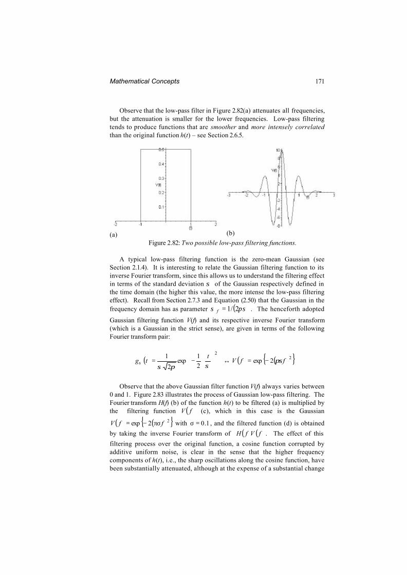
Observe that the low-pass filter in Figure 2.82(a) attenuates all frequencies,but the attenuation is smaller for the lower frequencies. Low-pass filteringtends to produce functions that are smoother and more intensely correlatedthan the original function h(t) – see Section 2.6.5.

(a) (b)

Figure 2.82: Two possible low-pass filtering functions.

A typical low-pass filtering function is the zero-mean Gaussian (seeSection 2.1.4). It is interesting to relate the Gaussian filtering function to itsinverse Fourier transform, since this allows us to understand the filtering effectin terms of the standard deviation σ of the Gaussian respectively defined inthe time domain (the higher this value, the more intense the low-pass filteringeffect). Recall from Section 2.7.3 and Equation (2.50) that the Gaussian in thefrequency domain has as parameter ( )πσσ 2/1=f . The henceforth adopted

Gaussian filtering function V(f) and its respective inverse Fourier transform(which is a Gaussian in the strict sense), are given in terms of the followingFourier transform pair:

( ) ( ) ( ){ }22

2exp2

1exp

2

1ffV

ttg πσ

σπσσ −=↔

−=

Observe that the above Gaussian filter function V(f) always varies between0 and 1. Figure 2.83 illustrates the process of Gaussian low-pass filtering. TheFourier transform H(f) (b) of the function h(t) to be filtered (a) is multiplied bythe filtering function ( )fV (c), which in this case is the Gaussian

( ) ( ){ }22exp ffV πσ−= with 1.0=σ , and the filtered function (d) is obtained

by taking the inverse Fourier transform of ( ) ( )fVfH . The effect of this

filtering process over the original function, a cosine function corrupted byadditive uniform noise, is clear in the sense that the higher frequencycomponents of h(t), i.e., the sharp oscillations along the cosine function, havebeen substantially attenuated, although at the expense of a substantial change


in the amplitude of h(t). An additional discussion about Gaussian filtering, inthe context of contour processing, is presented in Section 7.2.3.

-2 -1 0 1 2

-1

0

1

t

h (t )

- 2 0 - 1 0 0 1 0 2 0

0

0.2

0.4

f

H ( f)

- 2 0 - 1 0 0 1 0 2 0

0.2

0.4

0.6

0.8

1

f

V (f )

-2 -1 0 1 2-1

-0.5

0

0.5

t

q (t )

- 2 0 - 1 0 0 1 0 2 00

0.2

0.4

Q (f )

( a )

(d )

(b )

(c)

(e )

Figure 2.83: The function h(t) to be low-pass filtered (a), its respective Fouriertransform (b), the filtering function (in Fourier domain) (c), the filtered function

q(t) (d), and its respective Fourier transform (e).

The second class of filters, known as high-pass filters, act conversely tothe low-pass filters, i.e., by attenuating the magnitude of the low frequencycomponents of the signal, while the higher frequency components are allowedto pass. Such an attenuation should again be understood in relative terms.An example of high-pass filter is the complemented Gaussian V(f), defined as

( ) ( ) ( ) ( ){ }22

2exp12

1exp

2

1ffV

tttg πσ

σπσδσ −−=↔

−−=

It is interesting to observe that the complemented Gaussian filter functionalways varies between 0 and 1. This function is illustrated in Figure 2.84 for σ= 0.25.

As illustrated in Figure 2.85, a high-pass filter tends to accentuate the mostabrupt variations in the function being filtered, i.e., the regions where thederivative magnitude is high (in image processing and analysis, such abruptvariations are related to the image contrast). In other words, high-passfiltering reduces the correlation and redundancy degree in the original signal.


called deconvolution (this follows from the fact that the filtering process canbe alternatively understood as a convolution in the time space). If the originalfunction h(t) was filtered by a function V(f), yielding q(t), we may attempt torecover the original function by dividing the Fourier transform Q(f) of thefiltered function by the filter function V(f) and taking the inverse Fouriertransform as the result. Thus, the sought recovered function would be

obtained as ( ) ( ) ( ){ }fVfQth /1−ℑ= . However, this process is not possible

whenever V(f) assumes zero value. In practice, the situation is complicated bythe presence of noise in the signal and numeric calculation. Consequently,effective deconvolution involves more sophisticated procedures such asWiener filtering (see, for instance, [Castleman, 1992]).

2.7.5 The Discrete One-Dimensional Fourier TransformIn order to be numerically processed by digital computers, and to becompatible with the discrete signals produced by digital measuring systems,the Fourier transform has to be reformulated into a suitable discrete version,henceforth called discrete Fourier transform – DFT.

First, the function gi to be Fourier transformed is assumed to be a uniformlysampled (spaced by t∆ ) series of measures along time, which can be modelledin terms of multiplication of the original, continuous function ( )tg~ with the

sampling function ( ) ( )∑∞

−∞=∆ ∆−=Ψ

it titt δ . Second, by being the result of some

measuring process (such as the recording of a sound signal) the function gi isassumed to have finite duration along the time domain, let us say from time

tia a ∆= to tib b ∆= . The function gi is henceforth represented as

( )tigg i ∆= ~

Observe that the discrete function gi can be conveniently represented interms of the vector ( )

bbaa iiiiiii gggggggg ,,,,,,,, 1111 −+−+= LLr

. Figure

2.89 illustrates the generic appearance (i.e., sampled) of the function gi.


fttf

N∆∆

=∆∆= 1/1

Observe that we have ( )ftN ∆∆= /1 instead of ( ) 1/1 +∆∆= ftN because

we want to avoid repetition at the extremity of the period, i.e., the function issampled along the interval [a, b). The number M of sampling points in anyperiod of the output function H(f) is similarly given by

ftf

tM

∆∆=

∆∆

=1/1

By considering N = M, i.e., the number of sampling points representing theinput and output DFT functions are the same (which implies vectors of equalsizes in the DFT), we have

ftMN

∆∆== 1

(2.53)

Since the input function is always periodical, the DFT can be numericallyapproximated in terms of the Fourier series, which can be calculated byconsidering any full period of the input function h(t). In order to benumerically processed, the Fourier series given by Equation (2.47) can berewritten as follows. First, the integral is replaced by the sum symbol and thecontinuous functions are replaced by the above sampled input and outputfunctions. In addition, this sum is multiplied by t∆ because of the numericalintegration and the relationship Lfn 2= is taken into account, yielding

( ) ( )∫ =

−==∆= =

L

Lfnk L

ntjth

LcfkGG

2

02 exp

2

1 π

= ( ) ( )( )=

∆

−∆∆ ∑−

=

1

0

2exp

2

1 N

i L

tiLfjtih

Lt

π

( ) ( )( ){ }∑−

=∆∆−∆∆=

1

0

2exp2

1 N

i

tifkjtihL

t π

Observe that we have considered the time interval [0, 2L), in order to avoid

redundancies. By considering the input function as having period f

L∆

= 12 ,

we obtain

( ) ( ) ( )( ){ }∑−

=∆∆−∆∆∆=∆=

1

0

2expN

ik tifkjtihftfkHH π


Now, from Equation (2.53) we have N

ft1

=∆∆ , which implies that

( ) ( )∑−

=

−∆=∆=

1

0

2exp

1 N

ik N

ikjtih

NfkHH

π(2.54)

This equation, which is commonly known as the discrete Fouriertransform equation, allows us to numerically estimate the Fourier series of theperiodical function h(t). It is easily verified that the computational execution ofEquation (2.54) for each specific value of k demands N basic steps, beingtherefore an algorithm of complexity order O(N). Since the complete Fourierseries involves N calculations of this equation (i.e., k = 0, 1, … , N-1), theoverall number of basic operations in the DFT algorithm is of O(N2).

2.7.6 Matrix Formulation of the DFTEquation (2.54) can be compactly represented in matrix form, which isdeveloped in the following. By defining the abbreviations

−=

N

ikjw ik

π2exp, , ( )tihhi ∆= , and ( )fkHH k ∆= ,

Equation (2.54) can be rewritten as

∑−

=

=1

0,

1 N

iiikk hw

NH (2.55)

Before proceeding with the derivation of the matrix form of the DFT, it isinteresting to have a closer look at the discretized kernel function

−=

N

ikjw ik

π2exp, . Let us introduce ikki ww ,= and observe that

kiik ww ,, = ; for instance 2,21,44,14 wwww === . From Section 2.1, it is easy

to see that the complex exponential kernel function kiw , in the above equation

can be understood as the sequence of complex points uniformly distributed


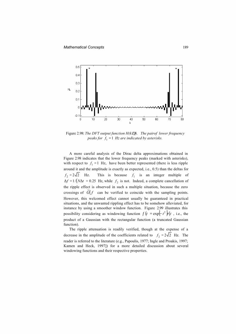
Figure 2.98: The DFT output function H(k∆f). The pairof lower frequencypeaks for 11 =f Hz are indicated by asterisks.

A more careful analysis of the Dirac delta approximations obtained inFigure 2.98 indicates that the lower frequency peaks (marked with asterisks),with respect to 11 =f Hz, have been better represented (there is less ripple

around it and the amplitude is exactly as expected, i.e., 0.5) than the deltas for

222 =f Hz. This is because 1f is an integer multiple of

( ) 25.0/1 =∆=∆ tNf Hz, while 2f is not. Indeed, a complete cancellation of

the ripple effect is observed in such a multiple situation, because the zero

crossings of ( )fG~

can be verified to coincide with the sampling points.

However, this welcomed effect cannot usually be guaranteed in practicalsituations, and the unwanted rippling effect has to be somehow alleviated, forinstance by using a smoother window function. Figure 2.99 illustrates this

possibility considering as windowing function ( ) { } ( )trtt 2exp −=φ , i.e., the

product of a Gaussian with the rectangular function (a truncated Gaussianfunction).

The ripple attenuation is readily verified, though at the expense of a

decrease in the amplitude of the coefficients related to 222 =f Hz. The

reader is referred to the literature (e.g., Papoulis, 1977; Ingle and Proakis, 1997;Kamen and Heck, 1997]) for a more detailed discussion about severalwindowing functions and their respective properties.

Documents

Differentiable (analytical, or smooth) functions: ( )