Embed Size (px)
Citation preview
6 Differentiable functions
6.1 Some examples
In the previous chapter we studied continuous functions, functions for which a small change in the argument
produces a small change in the value of the function. In this chapter we will take a closer look at the change in the
value of a function determined by a change in its variable, by examining the rate at which the value of the function
is changing when we change the value of its variable.
Example 6.1 Suppose that you are driving a car along a straight road, and that the total distance traveled in ≥ 0hours is given by () = 2+50 kilometers (this means for example that after = 1 you drove (1) = 51 km, after
3 hours you drove (3) = 159 km, aso).
If you want to know your average speed for the first 3 hours of your trip, then you can compute
Average speed =change in position
change in time=
(3)− (0)
3− 0 = 55 km.
If you want to know your instantaneous speed at = 3 hours (the speed your were driving at = 3 hours after
starting the trip), you can proceed as follows. You first determine the average speed for the time interval [3 3 +∆],
that is
Average speed on [3 3 +∆] = (3 +∆)− (3)
3 +∆− 3
=(3 +∆)
2+ 50 (3 +∆)− ¡32 + 50 · 3¢
∆= 56 +∆
Next, you notice that if ∆ is very small, then the average speed on [3 3 +∆] is approximately equal to the in-
stantaneous speed at = 3. To make this approximations exact, you let ∆→ 0, so you obtain that the instantaneous
speed at = 3 is
Instantaneous speed at time 3 = lim∆→0
(3 +∆)− (3)
3 +∆− 3 = lim∆→0
(56 +∆) = 56 km/h.
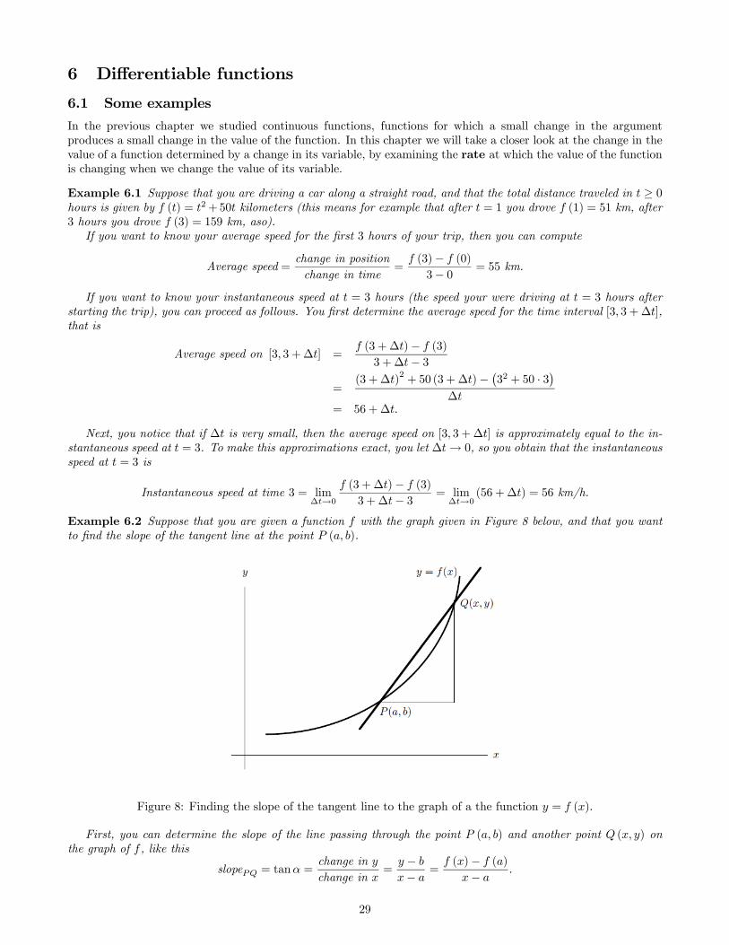
Example 6.2 Suppose that you are given a function with the graph given in Figure 8 below, and that you want
to find the slope of the tangent line at the point ( ).
Figure 8: Finding the slope of the tangent line to the graph of a the function = ().
First, you can determine the slope of the line passing through the point ( ) and another point ( ) on
the graph of , like this
slope = tan =change in
change in =
−
− =
()− ()
−
29
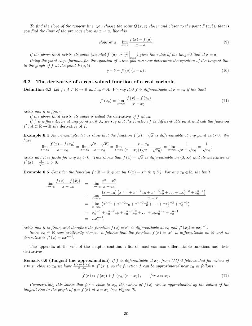
To find the slope of the tangent line, you choose the point ( ) closer and closer to the point ( ), that is
you find the limit of the previous slope as → , like this
slope at = lim→
()− ()
− . (9)
If the above limit exists, its value (denoted 0 () or
¯̄̄=
) gives the value of the tangent line at = .
Using the point-slope formula for the equation of a line you can now determine the equation of the tangent line
to the graph of at the point ( )
− = 0 () (− ) (10)
6.2 The derivative of a real-valued function of a real variable
Definition 6.3 Let : ⊂ R→ R and 0 ∈ . We say that is differentiable at = 0 if the limit
0 (0) = lim→0
()− (0)
− 0 (11)
exists and it is finite.
If the above limit exists, its value is called the derivative of at 0.
If is differentiable at any point 0 ∈ , we say that the function is differentiable on and call the function
0 : ⊂ R→ R the derivative of .
Example 6.4 As an example, let us show that the function () =√ is differentiable at any point 0 0. We
have
lim→0
()− (0)
− 0= lim
→0
√−√0− 0
= lim→0
− 0
(− 0)¡√
+√0¢ = lim
→0
1√+√0=
1√0
exists and it is finite for any 0 0. This shows that () =√ is differentiable on (0∞) and its derivative is
0 () = 1√, 0.
Example 6.5 Consider the function : R→ R given by () = ( ∈ N). For any 0 ∈ R, the limit
lim→0
()− (0)
− 0= lim
→0
− 0− 0
= lim→0
(− 0)¡−1 + −20 + −320 + + −20 + −10
¢− 0
= lim→0
¡−1 + −20 + −320 + + −20 + −10
¢= −10 + −20 0 + −30 20 + + 0
−20 + −10
= −10
exists and it is finite, and therefore the function () = is differentiable at 0 and 0 (0) = −10 .
Since 0 ∈ R was arbitrarily chosen, it follows that the function () = is differentiable on R and its
derivative is 0 () = −1.
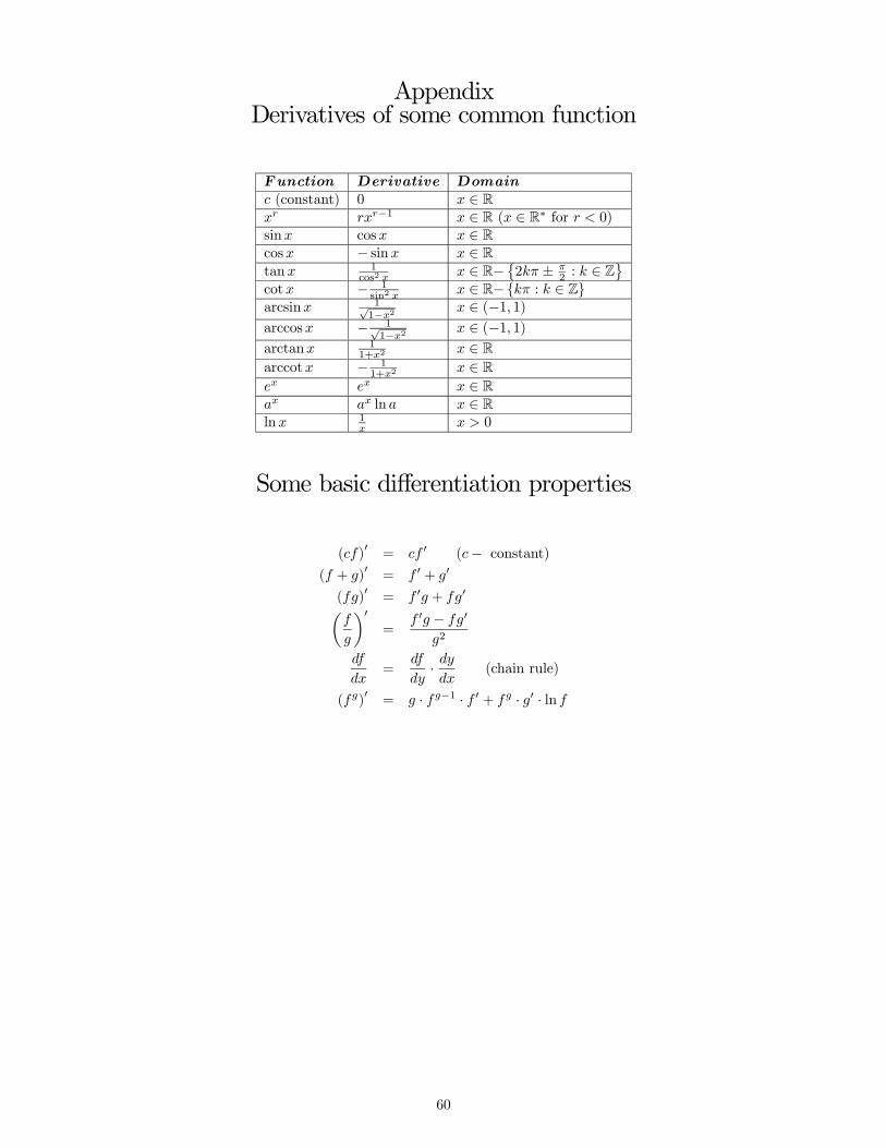
The appendix at the end of the chapter contains a list of most common differentiable functions and their
derivatives.
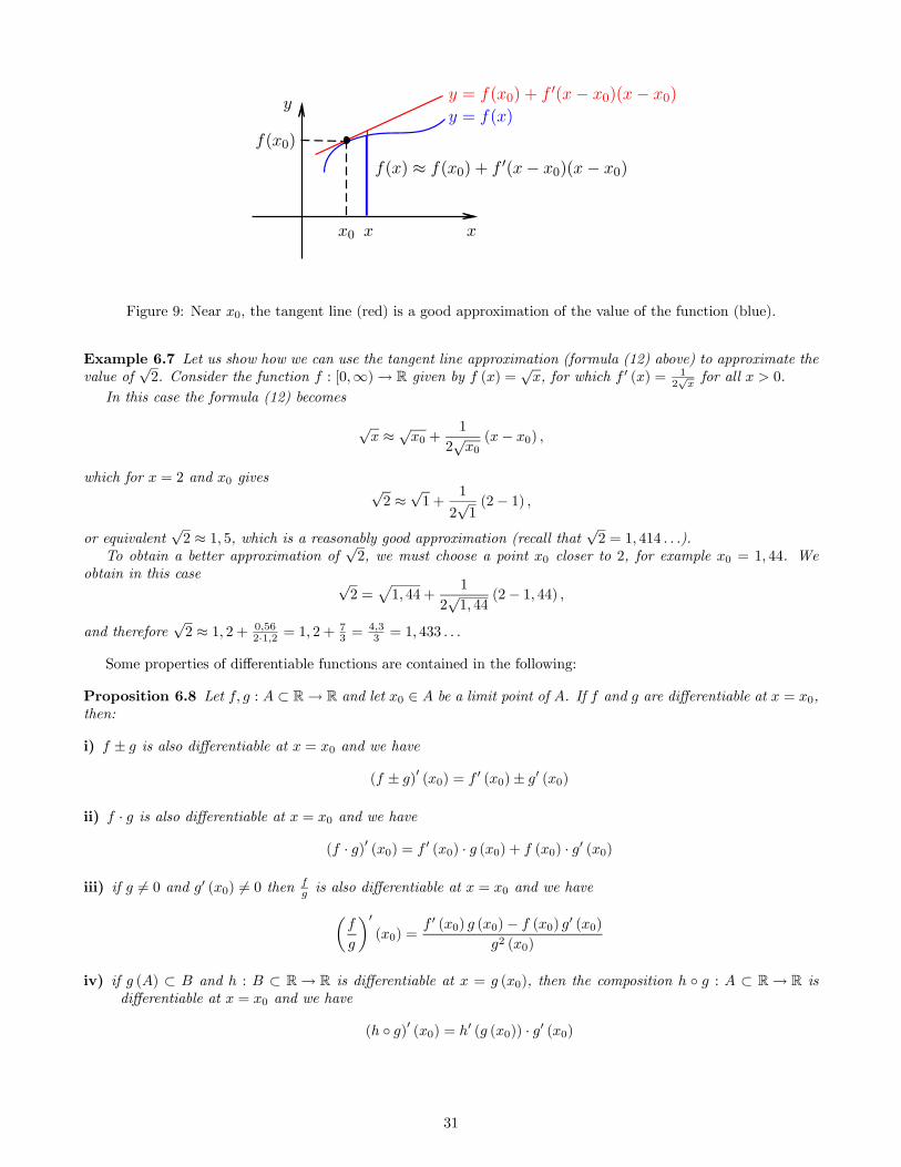
Remark 6.6 (Tangent line approximation) If is differentiable at 0, from (11) it follows that for values of
≈ 0 close to 0 we have()−(0)
−0 ≈ 0 (0), so the function can be approximated near 0 as follows:
() ≈ (0) + 0 (0) (− 0) for ≈ 0. (12)
Geometrically this shows that for close to 0, the values of () can be approximated by the values of the
tangent line to the graph of = () at = 0 (see Figure 9).
30
y = f(x)
x0
y = f(x0) + f ′(x − x0)(x − x0)
f(x0)
x
y
x
f(x) ≈ f(x0) + f ′(x − x0)(x − x0)
Figure 9: Near 0, the tangent line (red) is a good approximation of the value of the function (blue).
Example 6.7 Let us show how we can use the tangent line approximation (formula (12) above) to approximate the
value of√2. Consider the function : [0∞)→ R given by () =
√, for which 0 () = 1
2√for all 0.
In this case the formula (12) becomes
√ ≈ √0 + 1
2√0(− 0)
which for = 2 and 0 gives √2 ≈√1 +
1
2√1(2− 1)
or equivalent√2 ≈ 1 5, which is a reasonably good approximation (recall that √2 = 1 414 ).
To obtain a better approximation of√2, we must choose a point 0 closer to 2, for example 0 = 1 44. We
obtain in this case √2 =
p1 44 +
1
2√1 44
(2− 1 44)
and therefore√2 ≈ 1 2 + 056
2·12 = 1 2 +73= 43
3= 1 433
Some properties of differentiable functions are contained in the following:
Proposition 6.8 Let : ⊂ R→ R and let 0 ∈ be a limit point of . If and are differentiable at = 0,
then:
i) ± is also differentiable at = 0 and we have
( ± )0(0) = 0 (0)± 0 (0)
ii) · is also differentiable at = 0 and we have
( · )0 (0) = 0 (0) · (0) + (0) · 0 (0)
iii) if 6= 0 and 0 (0) 6= 0 then is also differentiable at = 0 and we haveµ
¶0(0) =
0 (0) (0)− (0) 0 (0)
2 (0)
iv) if () ⊂ and : ⊂ R→ R is differentiable at = (0), then the composition ◦ : ⊂ R→ R is
differentiable at = 0 and we have
( ◦ )0 (0) = 0 ( (0)) · 0 (0)
31
Proof. Follows by using the corresponding properties of limits. For example, to prove i):
lim→0
( ± ) ()− ( ± ) (0)
− 0= lim
→0
()− (0)
− 0± lim
→0
()− (0)
− 0= 0 (0)± 0 (0)
since the last two limit exist by hypothesis.
To prove ii), we write
lim→0
( · ) ()− ( · ) (0)− 0
= lim→0
µ ()− (0)
− 0 () + (0)
()− (0)
− 0
¶= lim
→0
()− (0)
− 0lim→0
() + (0) lim→0
()− (0)
− 0
= 0 (0) (0) + (0) 0 (0)
since by hypothesis are differentiable at 0 (also note that above we used the continuity of at 0: lim→0 () =
(0); since is differentiable at 0 it is also continuous at 0).
The rest of the proofs are similar, the reader is asked to try to write them.
Example 6.9 Using the properties of the derivatives (quotient rule), we can compute the derivative of the function
() = tan as follows
(tan)0=
µsin
cos
¶0=(sin)
0cos− sin (cos)0cos2
=cos cos− sin (− sin)
cos2 =sin2 + cos2
cos2 =
1
cos2
for any ∈ R for which cos 6= 0.
Example 6.10 To compute the derivative of the function () =¡3 + 1
¢2we can remove the parentheses and
then differentiate the result, as follows:
0 () =³¡3 + 1
¢2´0=¡6 + 23 + 1
¢0= 65 + 62 = 62
¡3 + 1
¢
The same derivative can be computed by using the chain rule, as follows:
0 () =³¡3 + 1
¢2´0= 2
¡3 + 1
¢2−1 · ¡3 + 1¢0 = 2 ¡3 + 1¢ · 32 = 62 ¡3 + 1¢ The following shows the relationship between differentiability and continuity:
Theorem 6.11 If : ⊂ R→ R is differentiable at 0 then is continuous at 0.
Proof. We will show that lim→0 () = (0). To do this, we write the limit as follows:
lim→0
() = (0) + lim→0
( ()− (0))
= (0) + lim→0
µ ()− (0)
− 0· (− 0)
¶= (0) + lim
→0
()− (0)
− 0· lim→0
(− 0)
= (0) + 0 (0) · 0= (0)
where we have used the fact that the last two limits exist and are finite (and therefore by a theorem, the limit of
the product is the product of the limits), concluding the proof.
As we will see, the derivative of a function is useful for finding the maximum /minimum value of a function. We
recall first the formal definition of an extremum point of a function:
Definition 6.12 Let : ⊂ R→ R and let 0 ∈ . We say that 0 is a:
i) local / relative minimum point for if for some 0 we have
(0) ≤ () ∈ ∩ (0 − 0 + ) (13)
32
ii) local / relative maximum point for if for some 0 we have
(0) ≤ () ∈ ∩ (0 − 0 + ) (14)
iii) local / relative extremum point for if 0 is either a local minimum or a local maximum point for .
If we have strict inequalities in (13) or (14), we say that 0 is a strict local minimum / local maximum / local
extremum for .
If the inequalities in (13) or (14) hold for any ∈ , then 0 is called an absolute (or global) minimum /
maximum / extremum point for .
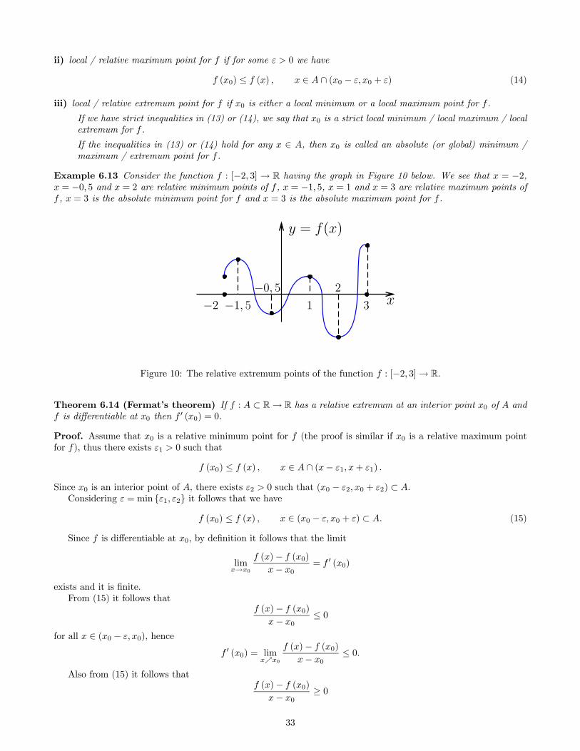
Example 6.13 Consider the function : [−2 3] → R having the graph in Figure 10 below. We see that = −2, = −0 5 and = 2 are relative minimum points of , = −1 5, = 1 and = 3 are relative maximum points of
, = 3 is the absolute minimum point for and = 3 is the absolute maximum point for .
y = f(x)
−0, 5x
2
31−1, 5−2
Figure 10: The relative extremum points of the function : [−2 3]→ R.
Theorem 6.14 (Fermat’s theorem) If : ⊂ R→ R has a relative extremum at an interior point 0 of and
is differentiable at 0 then 0 (0) = 0.
Proof. Assume that 0 is a relative minimum point for (the proof is similar if 0 is a relative maximum point
for ), thus there exists 1 0 such that
(0) ≤ () ∈ ∩ (− 1 + 1)
Since 0 is an interior point of , there exists 2 0 such that (0 − 2 0 + 2) ⊂ .
Considering = min {1 2} it follows that we have (0) ≤ () ∈ (0 − 0 + ) ⊂ (15)
Since is differentiable at 0, by definition it follows that the limit
lim→0
()− (0)
− 0= 0 (0)
exists and it is finite.
From (15) it follows that ()− (0)
− 0≤ 0
for all ∈ (0 − 0), hence
0 (0) = lim%0
()− (0)
− 0≤ 0.
Also from (15) it follows that ()− (0)
− 0≥ 0
33
for all ∈ (0 0 + ), hence
0 (0) = lim&0
()− (0)
− 0≥ 0.
We obtained
0 ≤ 0 (0) ≤ 0which shows 0 (0) = 0 as needed.
Remark 6.15 It is important to observe that in the theorem above is essential that 0 is an interior point of
(the domain of definition of the function ) and also that is differentiable at 0 (if is not differentiable at 0,
then 0 (0) is not defined, so it cannot equal 0!).To see this, consider the function : [1 2] → R defined by () = , and notice that 0 = 1 is a relative
minimum point for and 0 = 2 is a relative maximum point for (in fact these points are also the absolute
minimum and absolute maximum points for ). We see that is differentiable on [1 2] and 0 () = 1 for any
∈ [1 2]. In particular, 0 (1) = 0 (2) = 1 6= 0, which shows that the conclusion in Fermat’s theorem does not hold
(notice that 0 = 1 and 0 = 2 are not interior points of the domain [1 2] of ).
Theorem 6.16 (Rolle’s theorem) Let : [ ]→ R and assume that is continuous on [ ], differentiable on( ) and () = (). Then there exists ∈ ( ) such that 0 () = 0.
Proof. Since is continuous on [ ], by Weierstrass boundedness theorem (Theorem 4.9) is bounded and attains
its bounds on [ ], that is there exist ∈ [ ] such that
() ≤ () ≤ ( ) ∈ [ ]
If () = ( ) then is constant on [ ], and therefore 0 is identically zero on [ ], so we can choose any
∈ ( ) in this case.If () 6= ( ), then , cannot be both endpoints of [ ] (since by hypothesis () = ()), and
therefore at least one of or is an interior point of [ ].
Assuming is an interior point of [ ] (the proof is similar in the case when is an interior point of [ ]),
by Fermat’s theorem (Theorem 6.14) it follows that 0 () = 0, so we can choose = ∈ ( ) and conclude theproof.
A generalization of the above theorem is contained in the following:
Theorem 6.17 (Lagrange’s theorem) Let : [ ]→ R and assume that is continuous on [ ] and differen-tiable on ( ). Then there exists ∈ ( ) such that
0 () = ()− ()
− (16)
Proof. Consider the function : [ ]→ R defined by
() = ()− ()− ()
− (− )
Since is continuous on [ ] and differentiable on ( ), is also continuous on [ ] and differentiable on
( ), and we have
() = () = ()
By Rolle’s theorem (Theorem 6.16) there exists ∈ ( ) such that 0 () = 0, and since
0 () =µ ()− ()− ()
− (− )
¶0= 0 ()− ()− ()
−
we obtain equivalent
0 ()− ()− ()
− = 0
which proves the claim.
As a consequence, we have the following result which is useful in practice, for showing a function is monotone:
34
Proposition 6.18 Assume : [ ]→ R is continuous on [ ] and differentiable ( ).
i) If 0 () ≥ 0 for ∈ ( ) then is increasing on [ ];
ii) If 0 () ≤ 0 for ∈ ( ) then is decreasing on [ ].
iii) If 0 () = 0 for ∈ ( ) then is constant on [ ].
Proof. i) For arbitrary points 12 ∈ [ ] with 1 2, applying Theorem 6.17 to the function on the interval
[1 2] we obtain that there exists ∈ (1 2) such that
0 () = (2)− (1)
2 − 1
By hypothesis, the left side in the above equality is positive, so the right side must also be positive, and therefore
(since 2 − 1 0) we obtain (2)− (1) ≥ 0. We showed that (1) ≤ (2) for any 12 ∈ [ ] with 1 2
which shows that is increasing on [ ].
ii) A similar proof shows that in this case we have
(1) ≥ (2) for any 12 ∈ [ ] with 1 2
and therefore is decreasing on [ ] in this case.
iii) Similarly, for arbitrarily fixed points 12 ∈ [ ] with 1 2 we obtain that there exists ∈ ( ) such that (2)− (1)
2 − 1= 0 () = 0
and therefore (1) = (2). Since 12 ∈ [ ] were arbitrarily chosen, it follows that must be constant on [ ],concluding the proof.
Example 6.19 Consider the function () = 3. It is easy to see that is continuous and differentiable on R,and 0 () = 32 ≥ 0 for any ∈ R. By the previous theorem it follows that the function () = 3 is increasing
on R (it can be shown that it is in fact strictly increasing).
A generalization of Lagrange’s theorem is contained in the following:
Theorem 6.20 (Cauchy’s theorem) Let : [ ] → R and assume that and are continuous on [ ],
differentiable on ( ) and 0 () 6= 0 for ∈ ( ). Then ()− () 6= 0 and there exists ∈ ( ) such that 0 ()0 ()
= ()− ()
()− ()(17)
Proof. First note that applying Lagrange’s theorem to the function , there exists a point 1 ∈ ( ) such that ()− ()
− = 0 (1) 6= 0
and therefore () 6= (), which proves the first part of the claim.
Proceeding as in the proof of Lagrange’s theorem, we consider the function : [ ]→ R defined by
() = ()− ()− ()
()− ()( ()− ())
and we observe that since and are continuous on [ ] and differentiable on ( ), is also continuous on [ ]
and differentiable on ( ), and we have
() = () = ()
Applying Rolle’s theorem to the function we obtain that there exists ∈ ( ) such that 0 () = 0, and since
0 () = 0 ()− ()− ()
()− ()0 ()
35
we obtain equivalent
0 ()− ()− ()
()− ()0 () = 0
Dividing by 0 () 6= 0, we obtain 0 ()0 ()
= ()− ()
()− ()
concluding the proof.
As an application of Cauchy’s theorem, we will derive the following result, useful for computing limits of the
type 00:
Theorem 6.21 (L’Hôpital’s rule) Let : [ ] → R and 0 ∈ [ ]. If and are continuous on [ ] and
differentiable on ( )− {0}, 0 () 6= 0 for ∈ ( )− {0} and (0) = (0) = 0, then
lim→0
()
()= lim
→0
0 ()0 ()
(18)
provided the last limit exists.
Proof. We will consider just the case when the limit
lim→0
0 ()0 ()
= ∈ R
is finite (the case when = ±∞ can be proved similarly).
By the definition of the limit it follows that given 0 there exists 0 such that¯̄̄̄ 0 ()0 ()
−
¯̄̄̄ for all ∈ [ ] with 0 |− 0| (19)
Applying Cauchy’s theorem to the functions and on the interval with endpoints and 0 ([ 0] if 0,
respectively [0 ] if 0) we obtain that there exists a point = (the point depends on the choice of )
between and 0 that ()− (0)
()− (0)=
0 ()0 ()
Since (0) = (0) = 0 we obtain equivalent
()
()=
0 ()0 ()
and therefore we obtain ¯̄̄̄ ()
()−
¯̄̄̄=
¯̄̄̄ 0 ()0 ()
−
¯̄̄̄
for some point between and 0.
For ∈ [ ] with 0 |− 0| , since the point is between and 0, we also have 0 | − 0| ,
and therefore by (19) we obtain¯̄̄̄ ()
()−
¯̄̄̄=
¯̄̄̄ 0 ()0 ()
−
¯̄̄̄ for all ∈ [ ] with 0 |− 0|
which by the definition with of the limit shows that
lim→0
()
()=
concluding the proof.
36
Remark 6.22 (Extensions’s of L’Hôpital’s rule) Choosing = (or = ) in the above proof, we see that
the limit in the above theorem becomes the right (left) limit
lim→
()
()= lim
&
()
()
µrespectively lim
→
()
()= lim
%
()
()
This observation shows that L’Hôpital’s rule holds for sided limits (left / right limits at a point).
It can be shown that the above theorem holds in the case when 0 = ±∞.It can also be shown that L’Hôpital’s rule holds in the case ±∞
±∞ , that is in the case when lim→0 () =
lim→0 () = ±∞.
Example 6.23 As an example, let us compute the limit
lim→0
1 + −
2
We see that the limit is of the type 00and the functions involved satisfy the hypothesis of L’Hôpital’s rule above.
Applying the theorem we obtain
lim→0
1 + −
2= lim
→0(1 + − )
0
(2)0 = lim
→01−
2
Applying again the theorem (the resulting limit is also of the type 00), we obtain
lim→0
1 + −
2= lim
→01−
2= lim
→0(1− )
0
(2)0 = lim
→0−2
= −12
When applying L’Hôpital’s rule, it is essential to check that the limit on the right of (18) exists. Applying
L’Hôpital’s rule without checking that this limit exist, may lead to erroneous conclusions, as shown in the example
below:
Example 6.24 Consider the limit
lim→∞
+ sin
It is not difficult to see that− 1≤ + sin
≤ + 1
0
and therefore
1 = lim→∞
− 1≤ lim
→∞+ sin
≤ lim
→∞+ 1
= 1
which shows that
lim→∞
+ sin
= 1
Applying (incorrectly!) L’Hôpital’s rule we obtain
lim→∞
+ sin
= lim
→∞(+ sin)
0
()0 = lim
→∞1 + cos
1= lim
→∞1 + cos
limit which does not exist.
The above example shows that applying incorrectly L’Hôpital’s rule (without checking that the limit is indeed
of the type 00or ±∞±∞ , or without checking that the limit on the right exists), we may obtain erroneous conclusions.
37
6.2.1 Higher order derivatives
The definition of the derivative in Definition 6.3 can be extended to higher order derivatives, as follows:
Definition 6.25 Let : ⊂ R→ R and let 0 ∈ 5 . If the derivative 0 : ⊂ R→ R exists, we define the secondderivative of at 0 by
00 (0) = lim→0
0 ()− 0 (0)− 0
(20)
provided the limit exists.
If the above limit exists and it is also finite, we say that the function is twice differentiable at 0.
If is twice differentiable at any point 0 ∈ , we say that the function is twice differentiable on and call
the function 00 : ⊂ R→ R the second derivative of .
The above definition can be extended inductively, to any ∈ N, as follows:
Definition 6.26 Let : ⊂ R→ R and let 0 ∈ be an accumulation point of . If is times differentiable
on , we define the + 1 derivative of at 0 by
(+1) (0) = lim→0
() ()− () (0)
− 0(21)
provided the limit exists.
If the above limit exists and it is also finite, we say that the function is + 1 times differentiable at 0.
If is +1 times differentiable at any point 0 ∈ , we say that the function is +1 times differentiable on
and call the function (+1) : ⊂ R→ R the + 1 derivative of .
Remark 6.27 There are several notations in the literature for the derivative of a function. The most common is
perhaps Lagranges’s prime notation of the derivative, that is
(0) 0 (0) 00 (0) 000 (0)
or
(0) (1) (0)
(2) (0) (3) (0)
Another notation used (mostly in Physics) is Newton’s dot notation of the derivative, especially to denote
derivatives with respect to time:
(0) ̇ (0) ̈ (0) ... (0)
The prime and dot notations are difficult to read in the case when we want to indicate for example a fifth order
derivative. Leibniz’s differential notation
(0)
(0)
2
2(0)
3
3(0)
or Euler’s notation
(0) (0) 2 (0)
3 (0)
are useful in such situations.
We saw in Remark 6.6 that if : ⊂ R→ R is differentiable at the point 0 ∈ , then can be written
() = (0) + 0 (0) (− 0) + () (− 0) ∈
and moreover lim→0 () = 0. The next result shows that a similar representation holds if the function is
several times differentiable at 0. We have the following.
Theorem 6.28 (Taylor’s formula) Let : ( ) ⊂ R→ R be a function which is + 1 times differentiable onthe interval ( ) and let 0 ∈ ( ). Then for each ∈ ( ) there exists a point between 0 and such that
() = (0) + 0 (0)1!
(− 0) + 00 (0)2!
(− 0)2+ +
() (0)
!(− 0)
+
(+1) ()
(+ 1)!(− 0)
+1(22)
5The point 0 ∈ should not be an isolated point of .
38
Proof. If = 0 then we can choose = 0 and the claim follows.
For 6= 0, if we consider the number ∈ R given by
() = (0) + 0 (0)1!
(− 0) + 00 (0)2!
(− 0)2+ +
() (0)
!(− 0)
+ · (− 0)
+1 (23)
in order to prove the claim we have to show the existence of between 0 and such that
= (+1) ()
(+ 1)!
To prove this, consider the function : → R defined by
() = () + 0 ()1!
(− ) + 00 ()2!
(− )2+ +
() ()
!(− )
+ · (− )
+1
and note that since by hypothesis is + 1 times differentiable on , the function is differentiable on .
Also, note that
() = ()
and
(0) = (0) + 0 (0)1!
(− 0) + 00 (0)2!
(− 0)2+ +
() (0)
!(− 0)
+ · (− 0)
+1= ()
by using the definition of the constant (formula (23)).
We can therefore apply Rolle’s theorem to the function , and deduce the existence of a number between 0and , such that
0 () = 0.
Computing the derivative of we obtain:
0 () =
µ () +
0 ()1!
(− ) + 00 ()2!
(− )2+ +
() ()
!(− )
+ · (− )
+1
¶= 0 () +
µ 00 ()1!
(− )− 0 ()1!
¶+
µ 000 ()2!
(− )2 − 00 ()
1!(− )
¶+ +
+
µ (+1) ()
!(− )
− () ()
(− 1)! (− )−1
¶− · (+ 1) (− )
= (+1) ()
!(− )
− · (+ 1) (− )
and therefore 0 () = 0 gives (+1) ()
!(− )
− · (+ 1) (− )= 0
and since − 6= 0 (recall that by Rolle’s theorem is strictly between 0 and ), we obtain equivalent
= (+1) ()
(+ 1)!
concluding the proof.
Definition 6.29 Under the assumptions of the previous theorem, the polynomial () defined by
() = (0) + 0 (0)1!
(− 0) + 00 (0)2!
(− 0)2+ +
() (0)
!(− 0)
(24)
is called the Taylor polynomial of order of at the point 0, and () defined by
() = (+1) ()
(+ 1)!(− 0)
+1(25)
is called the Taylor remainder of order of at the point 0.
39
Remark 6.30 Note that in the case = 0, the above theorem becomes Lagrange’s theorem (Theorem 6.17).
Remark 6.31 The formula (22) in the previous theorem can be written in the form
() = () + () =
X=0
() (0)
!(− 0)
+
(+1) ()
(+ 1)!(− 0)
+1
or equivalently (with the substitution = 0 + ):
(0 + ) = (0 + ) + (0 + ) =
X=0
() (0)
! +
(+1) ()
(+ 1)!+1
called the Taylor formula of order of at the point 0.
As an application of the Taylor formula, we obtain the following sufficient condition for the extremum of a
function:
Theorem 6.32 Let : ( ) ⊂ R→ R be a function which is + 1 ≥ 2 times differentiable with (+1) ()
continuous on the interval ( ), 0 ∈ ( ) and assume that
0 (0) = 00 (0) = = () (0) = 0 and (+1) (0) 6= 0
Then if:
i) + 1 is an even number, has a local extremum at 0. More precisely, if (+1) (0) 0 then 0 is a local
minimum point for , and if (+1) (0) 0 then 0 is a local maximum point for ;
ii) + 1 is an odd number, does not have a local extremum at 0.
Proof. Under the assumption of the theorem, the Taylor formula of order for at 0 becomes
() = (0) + (+1) ()
(+ 1)!(− 0)
+1
where is a point between 0 and .
If + 1 is an even number, from the above equality we see that ()− (0) has the sign of (+1) () (since
(− 0)+1 ≥ 0 for any ∈ ( )), and therefore for any ∈ (0 − 0 + ) with 0 sufficiently small,
()− (0) has the sign of (0) (recall that is between 0 and ).
It follows that if (0) is a local minimum if (0) ≥ 0, respectively a local maximum if (0) ≤ 0.If + 1 is odd, the same reasoning shows that () − (0) takes both positive and negative values in any
interval (0 − 0 + ) with 0, so 0 is not a relative extremum for in this case.
Example 6.33 Consider the functions : R→ R given by () = sin2 and () = sin2 .
It is easy to see that
0 (0) = 0 and 00 (0) = 2 6= 0and
0 (0) = 00 (0) = 0 and 000 (0) = 6 6= 0and therefore by the above theorem it follows that 0 = 0 is a relative minimum point for (+ 1 = 2 is an even
number and 00 (0) 0), but it is not a relative extremum point for (+ 1 = 3 is an odd number).
6.3 The derivative of a real-valued function of a vector variable
Recall that a point ∈ R is a -dimensional vector, and we will write = (1 ), where 1 are thecorresponding coordinates. In case of a point 0 ∈ R, we will write its coordinates as 01 0 (the superscript0 is does not mean the power zero in this case), that is 0 =
¡01
0
¢.
Identifying a point ∈ R with its coordinates (1 ), for a function : ⊂ R→ R we will write either () or (1 ).
40
Definition 6.34 (Definition of partial derivatives) We say that the function : ⊂ R → R has a partialderivative at the point 0 ∈ with respect to the th variable if the limit
lim→0
¡01
0−1
0+1
0
¢− ¡01
0−1
0
0+1
0
¢ − 0
(26)
exists and it is finite. The value of the above limit is denoted by
(0) or 0(0) and it is called the partial
derivative of with respect to at the point x0.
Remark 6.35 The above definition says that in order to see if the function is differentiable at the point 0 =¡01
0
¢, we fix all its variables except for the th variable to the corresponding values of the point 0, thus
obtaining the function () = ¡01
0−1
0+1
0
¢; if the function is differentiable at the point 0 ,
then the function is differentiable with respect to the th variable at 0.
Example 6.36 Consider : R× (0∞) → R given by (1 2) = 31 ln2, where = (1 2) ∈ R×(0∞). It iseasy to see that has partial derivatives with respect to both variables at any point 0 ∈ R×(0∞). For example,considering 0 =
¡5 2
¢, we have
1
¡5 2
¢= lim
1→5¡1
2¢−
¡3 2
¢1 − 5
= lim1→5
31 ln 2 − 53 ln 21 − 5
= 2 lim1→5
31 − 531 − 5
= 2 lim1→5
(1 − 5)¡21 + 51 + 5
2¢
1 − 5= 2 lim
1→521 + 51 + 5
2
= 2 · 3 · 52= 150
Similarly it can be shown that for an arbitrary point 0 =¡01
02
¢ ∈ R× (0∞) we have
1
¡01
02
¢= 3
¡01¢2ln02 and
2
¡01
02
¢=
¡01¢3
02
Remark 6.37 The above exercise shows that the partial derivatives of with respect to can be calculated by
considering that the remaining variables of are constant, and differentiating with respect to .
Proposition 6.38 (Relation between partial derivatives and continuity) If : ⊂ R → R has partial
derivative with respect to th variable at the point 0, then is continuous with respect to the th variable at this
point (but may not be continous with respect to all variables! See the following example).
If all the partial derivatives of : ⊂ R → R exist near the point 0 and they are bounded, then is continuousat 0.
Proof. If has partial derivative with respect to the variable at the point 0 =¡01
0
¢, then
lim→0
¡01
0−1
0+1
0
¢=
= lim→0
¡01
0−1
0+1
0
¢− ¡01
0−1
0
0+1
0
¢ − 0
· ¡ − 0¢+
¡01
0−1
0
0+1
0
¢=
(0) ·
¡0 − 0
¢+ (0)
= (0)
and therefore is continous with respect to the variable at the point 0, proving the first part of the statement.
41
If all the partial derivatives of exist near 0 and they are bounded, then writing
()− (0) = (1 2 3 )− ¡01 2 3
¢+
¡01 2 3
¢− ¡01
02 3
¢+
¡01
02 3
¢− ¡01
02
03
¢+
+¡01
02
03
¢− ¡01
02
03
0
¢and applying Lagrange theorem to each difference (since the function have partial derivatives with respect to all
variables), we obtain
()− (0) =
1(∗1 2 3 )
¡1 − 01
¢+
2
¡01
∗2 3
¢ ¡2 − 02
¢+
3
¡01
02 ∗3
¢ ¡3 − 03
¢+
+
1
¡01
02
03
∗
¢ ¡ − 0
¢
Since the partial derivatives are assumed bounded (say by a constant 0), we obtain
| ()− (0)| ≤¯̄1 − 01
¯̄+
¯̄2 − 02
¯̄+ +
¯̄ − 0
¯̄for all = (1 ) close enough to 0 =
¡01
0
¢, and therefore
0 ≤ lim→0
| ()− (0)| ≤ lim→0
¯̄1 − 01
¯̄+
¯̄2 − 02
¯̄+ +
¯̄ − 0
¯̄= 0
which shows that
lim→0
() = (0)
By definition, this shows that is continous at 0, concluding the proof.
The next example shows that even if all partial derivatives exist, the function may not be continous (the
hypothesis that the partial derivatives are bounded is therefore essential in the previous theorem).
Example 6.39 Consider the function : R2 → R defined by
( ) =
½ 22+2
( ) 6= (0 0)0 ( ) = (0 0)
Using the definition it can be checked that has partial derivatives at any point in R2 − {(0 0)}. Since
lim→0
( 0)− (0 0)
− 0 = lim→0
2··02+02
− 0− 0 = lim
→00
= 0
it follows that has partial derivative with respect to at (0 0) and (0 0) = 0. A similar proof shows that the
partial derivative of with respect to at (0 0) exists and (0 0) = 0, and therefore has partial derivatives at
any point in R2.However, is not continuous at (0 0), since lim()→(00) ( ) does not exist. To see this, compute the limit
on two different directions, say along = and = −: in the first case we obtain lim→0 ( ) = lim→0 2··2+2
= 2
and in the second case we obtain lim→0 (−) = lim→02··(−)2+(−)2 = −2, and therefore lim()→(00) ( ) does
not exist.
The previous example also shows that the partial derivatives is not the “correct” extension of the notion of
differentiability of functions of one real variable to functions of several variables, in the sense that a function may
have partial derivatives at a point but it may fail to be continuous at this point (for the correct definition of
differentiability we would expect that if a function is differentiable at a point then it is also continuous at this
point). The “correct” extension of differentiability is given by the following:
42
Definition 6.40 (Definition of differentiability) We say that the function : ⊂ R → R is differentiable
at the interior point 0 ∈ if there exists = (1 ) ∈ R and a function : ⊂ R → R with
lim→0 () = (0) = 0 such that
() = (0) + · (− 0) + () k− 0k ∈ (27)
Remark 6.41 For example, in the case = 3, the above condition for differentiability of a function (1 2 3)
is
(1 2 3) = ¡01
02
03
¢+ 1
¡1 − 01
¢+ 2
¡2 − 02
¢+ 3
¡3 − 03
¢+ (1 2 3)
q(1 − 01)
2+ (2 − 02)
2+ (3 − 03)
2
Remark 6.42 Writing = 0 + , the above condition for differentiability can be written in the equivalent form
(0 + ) = (0) + · + (0 + ) kk 0 + ∈
The linear application 7−→ · = 11 + + is called the differential of at 0 and is denoted
(0) = · =X=1
(28)
It is easy to see that for any ∈ {1 } the function (1 ) = is differentiable in the sense of the
above definition (just consider = 1 and = 0 for 6= and (1 ) ≡ 0), and therefore
(0) =
X=1
= = 1 =
thus (0) = (0) = , = 1 .
We can therefore replace in the above definition of the differential of at 0, to get
(0) =
X=1
(0) ∈ R
or (without writing the variable ):
(0) =
X=1
(0)
or simply
=
X=1
where the constants are those in the Definition 6.40 of differentiability of .
The following proposition shows the connection between differentiability and continuity of a function:
Proposition 6.43 (Relation between differentiability and continuity) If : ⊂ R → R is differentiableat the interior point 0 of , then is continuous at the point 0.
Proof. If is differentiable at 0 ∈ , then there exists = (1 ) ∈ R and a function : ⊂ R → Rwith lim→0 () = (0) = 0 such that the relation (??) holds for any ∈ .
We obtain:
lim→0
() = lim→0
( (0) + · (− 0) + () k− 0k)= (0) + · (0 − 0) + (0) k0 − 0k= (0)
which shows that is continuous at 0.
The next example shows that the converse of the previous two theorems is not true in general (i.e., if a function
is continuous at a point it does not necessarily have partial derivatives at this point, and it is not necesssarily
differentiable at this point).
43
Example 6.44 Consider the function : R2 → R defined by ( ) = ||+ ||.The function is obviously continuous at (0 0) since
lim()→(00)
( ) = lim()→(00)
||+ || = 0 = (0 0)
but it does not have partial derivatives at (0 0):
lim→0
( 0)− (0 0)
− 0 = lim→0
||- does not exist,
and similarly
lim→0
(0 )− (0 0)
− 0 = lim→0
||- does not exist.
The function is also not differentiable at (0 0). If it were, then
( ) = (0 0) + 1+ 2 + ( )p2 + 2 ( ) ∈ R2
for some constants 1 2 ∈ R and a function ( ) with lim()→(00) ( ) = 0.Solving the above equation for the function ( ) and using the definition of the function we obtain
( ) =||+ ||− 1− 2p
2 + 2 ( ) 6= (0 0)
Since lim()→(00) ( ) = 0, in particular the limit of ( ) along the direction = would be zero, that is
0 = lim→0
||+ ||− 1− 2√2 + 2
= lim→0
2 ||− (1 + 2) √2 || = lim
→0
√2− (1 + 2) √
2 ||
Computing the above limit as % 0 we obtain√2 + 1+2√
2, and for & 0 we obtain
√2 − 1+2√
2. Since the
limit as → 0 exists, the sided limits must be equal, and therefore we must have 1 + 2 = 0. Replacing in the
above equation, we obtain
0 =√2
contradiction which shows that is not differentiable at (0 0).
The relation between differentiability and the partial derivatives of a function is given by the following:
Theorem 6.45 (Relation between differentiability and partial derivatives) If : ⊂ R → R is differ-entiable at an interior point 0 of , then has partial derivatives with respect to all variables at the point 0.
Conversely, if all partial derivatives of exist near the point 0 and they are continuous at the point 0, then
the function is differentiable at the point 0.
In both cases, the constants in the Definition 6.40 of differentiability of coincide with the partial derivatives
of at 0, that is =
(0).
Proof. First implication follows by the definition of differentiability (divide by −0 and take limits with → 0 ).
For the second implication, write
()− (0) = (1 2 3 )− ¡01 2 3
¢+
¡01 2 3
¢− ¡01
02 3
¢+
¡01
02 3
¢− ¡01
02
03
¢+
+¡01
02
03
¢− ¡01
02
03
0
¢
44
and apply Lagrange theorem to each difference (since the function have partial derivatives with respect to all
variables), to get
()− (0) =
1(∗1 2 3 )
¡1 − 01
¢+
2
¡01
∗2 3
¢ ¡2 − 02
¢+
3
¡01
02 ∗3
¢ ¡3 − 03
¢+
+
1
¡01
02
03
∗
¢ ¡ − 0
¢
for some points ∗ between ands 0 .
Considering the function : ⊂ R → R defined by (0) = 0 and
() =1
k− 0kX=1
µ
¡01
0−1
∗ +1
¢−
¡01
0−1
0
0+1
0
¢¶ ¡ − 0
¢
by the continuity of partial derivatives it follows6 that lim→0 () = 0 = (0) and we have
() = (0) +
X=1
(0) ·
¡ − 0
¢+ () k− 0k ∈
which shows that is differentiable at 0.
The next example shows that the hypothesis that the partial derivatives are continuous is essential in the previous
theorem, that is, it is possible that the function has partial derivatives but it is not differentiable.
Example 6.46 Consider the function : R2 → R defined by
( ) =
(||p2 + 2 6= 0
0 = 0
Since ¯̄̄̄
||p2 + 2
¯̄̄̄=||||p2 + 2 =
p2 + 2 → 0
as ( ) → (0 0) (and 6= 0), it follows that lim()→(00) ( ) = 0 = (0 0), and therefore the function is
continuous at (0 0).
The function has partial derivatives at (0 0):
(0 0) = lim
→0 ( 0)− (0 0)
− 0 = lim→0
0− 0− 0 = 0
and
(0 0) = lim
→0 (0 )− (0 0)
− 0 = lim→0
||p02 + 2
= lim
→0
|| ||
= 1
If were differentiable at (0 0), then
( ) = (0 0) + 1+ 2 + ( )p2 + 2 ( ) ∈ R2
for some constants 1 2 ∈ R and a function ( ) with lim()→(00) ( ) = 0.From the previous theorem it follows that 1 =
(0 0) = 0 and 2 =
(0 0) = 1, and solving the above
equation for ( ) we obtain
( ) =
|| −p
2 + 2 6= 0
6Note that since|−0 |k−0k ≤ 1, we have | ()| ≤
=1
01 0−1 ∗ +1 −
01
0−1
0
0+1
0
→0 as → 0 (recall that the points
∗ being between and 0 , we have
∗ → 0 as → 0).
45
ca
b
A
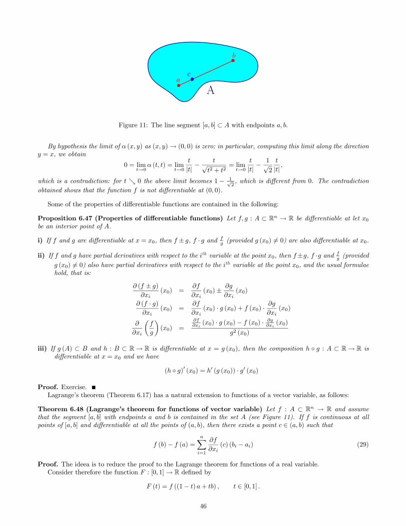
Figure 11: The line segment [ ] ⊂ with endpoints .
By hypothesis the limit of ( ) as ( )→ (0 0) is zero; in particular, computing this limit along the direction
= , we obtain
0 = lim→0
( ) = lim→0
|| −√
2 + 2= lim
→0
|| −1√2
||
which is a contradiction: for & 0 the above limit becomes 1 − 1√2, which is different from 0. The contradiction
obtained shows that the function is not differentiable at (0 0).
Some of the properties of differentiable functions are contained in the following:
Proposition 6.47 (Properties of differentiable functions) Let : ⊂ R → R be differentiable at let 0be an interior point of .
i) If and are differentiable at = 0, then ± , · and (provided (0) 6= 0) are also differentiable at 0.
ii) If and have partial derivatives with respect to the th variable at the point 0, then ±, · and (provided
(0) 6= 0) also have partial derivatives with respect to the th variable at the point 0, and the usual formulaehold, that is:
( ± )
(0) =
(0)±
(0)
( · )
(0) =
(0) · (0) + (0) ·
(0)
µ
¶(0) =
(0) · (0)− (0) ·
(0)
2 (0)
iii) If () ⊂ and : ⊂ R→ R is differentiable at = (0), then the composition ◦ : ⊂ R→ R is
differentiable at = 0 and we have
( ◦ )0 (0) = 0 ( (0)) · 0 (0)
Proof. Exercise.
Lagrange’s theorem (Theorem 6.17) has a natural extension to functions of a vector variable, as follows:
Theorem 6.48 (Lagrange’s theorem for functions of vector variable) Let : ⊂ R → R and assume
that the segment [ ] with endpoints and is contained in the set (see Figure 11). If is continuous at all
points of [ ] and differentiable at all the points of ( ), then there exists a point ∈ ( ) such that
()− () =
X=1
() ( − ) (29)
Proof. The ideea is to reduce the proof to the Lagrange theorem for functions of a real variable.
Consider therefore the function : [0 1]→ R defined by
() = ((1− ) + ) ∈ [0 1]
46
Applying Lagrange theorem (Theorem 6.17) to the function on the interval [0 1] ⊂ R, it follows that thereexists a point ∗ ∈ (0 1) such that
(1)− (0) = 0 (∗) (1− 0) or equivalent
()− () = 0 (∗)
Note that by the chain rule we have:
0 () =
( ((1− ) 1 + 1 (1− ) + ))
=
X=1
((1− ) 1 + 1 (1− ) + ) · ( − )
and therefore setting = (1− ∗) + ∗ ∈ ( ) gives the conclusion of the theorem.
6.3.1 Differentiability of compositions of functions
In practice, we often encounter functions which are composition of differentiable functions (for example sin¡2 + 2
¢,
2+3, etc). To differentiate such functions, we can use the following:
Theorem 6.49 (“Chain rule”) Let = ( ) : ⊂ R2 → R and = () = () : ⊂ R→ R such that( () ()) ∈ for all ∈ .
If the functions () () are differentiable at 0, and the function ( ) is differentiable at (0 0) =
( (0) (0)), then the composition function () = ( () ()) : → R is differentiable at 0 and we have
0 (0) =
(0 0)
(0) +
(0 0)
(0)
Proof. Since the function is differentiable at (0 0), by definition we have
( ) = (0 0) +
(0 0) (− 0) +
(0 0) ( − 0) + ( )
q(− 0)
2+ ( − 0)
2 ( ) ∈
for some function : ⊂ R2 → R with lim()→(00) ( ) = 0.Replacing in the above equality by () and by (), we obtain:
()− (0)
− 0=
( () ())− ( (0) (0))
− 0
=
(0 0)
()− (0)
− 0+
(0 0)
()− (0)
− 0
+ ( () ())
q( ()− (0))
2+ ( ()− (0))
2
− 0
Passing to limit with → 0, and using the fact that the functions () and () are differentiable, we obtain
lim→0
()− (0)
− 0=
(0 0) lim
→0
()− (0)
− 0+
(0 0) lim
→0
()− (0)
− 0
+ lim→0
( () ())
sµ ()− (0)
− 0
¶2+
µ ()− (0)
− 0
¶2=
(0 0)
0 (0) +
(0 0)
0 (0) + 0 ·q(0 (0))
2+ (0 (0))
2
=
(0 0)
0 (0) +
(0 0)
0 (0)
since by hypothesis lim()→(00) ( ) = 0 (note that since the functions () and () are differentiable at 0,
they are continuous at the point 0, and therefore as → 0 we have ( () ())→ ( (0) (0)) = (0 0)).
47
By definition, the above shows that the function is differentiable at the point 0 and we have
0 (0) =
(0 0)
0 (0) +
(0 0)
0 (0)
concluding the proof of the theorem.
Example 6.50 Consider the functions ( ) = 2 + 3, ( ) ∈ R2 and () = sin , () = 4, ∈ R. All thesefunctions are differentiable at any point in their domain of definition, and we have
= 2
= 32 0 () = cos and 0 () = 43.
By the above theorem it follows that the function () = ( () ()), ∈ R is differentiable at any point ∈ R,and we have
0 () =
( () ())0 () +
( () ()) 0 ()
= 2|(sin 4) · cos + 32¯̄(sin 4)
· 43
= 2 sin · cos + 3 ¡4¢2 · 43= 2 sin cos + 1211
Alternately, we can compute the derivative of the function by writing it explicitly in terms of that is
() = ( () ()) = ¡sin 4
¢= (sin )
2+¡4¢3= sin2 + 12
and differentiating with respect to
0 () = 2 sin cos + 1211
The above theorem shows that computing the derivative of a composition function by either of the two methods
above we get the same answer.
The above theorem can be generalized in several ways. First, if the function = (1 2 ) has variables
instead of just 2 variables, and each of them is a function of a variable ∈ R, then, as in the previous theorem,if all the functions involved are differentiable, the composition function () = (1 () 2 () ()) is also
differentiable, and we have
=
1· 1
+
2· 2
+ +
·
(30)
A second extension of the chain rule in the previous theorem is to the case when = ( ) and = ( )
are functions of two variables ∈ R. In this chase, if all the functions involved are differentiable, then thecomposition function ( ) = ( ( ) ( )) is also differentiable, and the partial derivatives of the function
with respect to and are given by
=
· +
·
(31)
and
=
· +
·
(32)
The most general case of the chain rule is the case when the function = (1 ) is a function of vari-
ables, and each variable = (1 ) is a function of variables 1 ∈ R. As an exercise, the reader isasked to write the partial derivatives of the composition function (1 ) = (1 (1 ) (1 ))
with respect to the variables 1 .
Example 6.51 Consider the function ( ) = + 2 + 3 and ( ) = + 2, ( ) = 2 + 3 and
( ) = 3 + 5, and let ( ) = ( ( ) ( ) ( )).
All the functions involved are differentiable, and we have
= 1
= 2
= 32
= 1
= 2
= 2
= 3
= 32
= 5
48
From the chain rule it follows that the function ( ) is differentiable, and the partial derivatives of with
respect to and are given by
=
· +
· +
·
= 1 · 1 + 2 · 2+ 32 · 32= 1 + 4
¡2 + 3
¢+ 9
¡3 + 5
¢22
and
=
· +
· +
·
= 1 · 2 + 2 · 3 + 32 · 5= 2 + 6
¡2 + 3
¢+ 15
¡3 + 5
¢2
as it can be checked directly by computing the partial derivatives of
( ) = ¡+ 2 2 + 3 3 + 5
¢= (+ 2) +
¡2 + 3
¢2+¡3 + 5
¢3
6.3.2 Gradient and directional derivatives
Definition 6.52 For a given unitary vector ∈ R (i.e. kk = 1), we define the directional derivative of the
function : ⊂ R → R in the direction at the point 0 ∈ by
(0) = lim
→0 (0 + )− (0)
if this limit exists.
We have the following:
Theorem 6.53 If the function : ⊂ R → R is differentiable at the interior point 0 of then the directionalderivative of in any direction at 0 exists, and we have
(0) = 1
1(0) + +
(0) = ∇ (0) ·
where ∇ (0) =³
1
(0)
(0)´.
Proof. Consider ∈ R an arbitrary unitary vector.Since the function is differentiable at the point 0, there exists a function : ⊂ R → R with lim→0 () =
0 such that we have:
(0 + ) = (0) +
1(0)
¡01 + 1 − 01
¢+ +
(0)
¡0 + − 0
¢+ (0 + )
q(01 + 1 − 01)
2+ + (0 + − 0)
2
= (0) +
1(0) · 1 + +
(0) · + (0 + ) ||
q21 + + 2
= (0) + ∇ (0) · + (0 + ) || since kk =
p21 + + 2 = 1.
We obtain
lim→0
(0 + )− (0)
= lim
→0∇ (0) · + (0 + )
||= ∇ (0) ·
since lim→0 () = 0 (and therefore lim→0 (0 + ) = 0) and¯̄̄||
¯̄̄= 1 is bounded.
The above shows that the directional derivative of at 0 in an arbitrary direction ∈ R exists and we have
(0) = ∇ (0) · = 1
1(0) + +
(0)
concluding the proof.
49
Definition 6.54 If the function : ⊂ R → R has partial derivatives, the vector
∇ =µ
1
¶with components equal to the partial derivatives of with respect to its variables is called the gradient of the function
.
Remark 6.55 (Geometric interpretation of directional derivative) The directional derivative (0) gives
the rate of change in the function when moving in the direction indicated by the vector . To see this, note that
the trajectory in the direction starting at the point 0 can be described by () = 0 + , ≥ 0. The value of thefunction at moment tt (if we think ≥ 0 as being the time) is given by ( ()) = (0 + ), and therefore the rate
of change in the value of the function (at time = 0) is
( ())
¯̄̄̄=0
= lim→0
( ())− ( (0))
= lim
→0 (0 + )− (0)
=
(0)
From the previous theorem we see that the rate of change in the function at the point 0 in an arbitrary
direction is
(0) = ∇ (0) · = k∇ (0)k kk cos = k∇ (0)k cos (33)
where is the angle between the vector and the gradient ∇ (0) of at the point 0.Remark 6.56 (Maximum and minimum rate of change) From the above relation we can see that the max-
imum rate of change in the value of the function is obtained in the direction of the gradient ∇ (0) (when = ∇ (0) the angle = 0 and therefore cos = 1), and the minimum rate of change in the value of the function
is obtained in the opposite direction of the gradient, that is in the direction −∇ (0) (in this case the angle = ,
and therefore cos = −1).
6.3.3 Higher order partial derivatives
Definition 6.57 If the function : ⊂ R → R has partial derivative
with respect to the variable near
the point 0 ∈ , and
has partial derivatives with respect to the variable , we define the second order partial
derivatives of at 0 (first with respect to , then with respect to ) by
2
(0) =
µ
¶(0) (34)
Remark 6.58 The second order partial derivative 2
above is sometimes denoted by .
The above definition can be extended inductively, that is, if has th order partial derivatives, we define the
(+ 1)stpartial derivative of as the partial derivative of the th partial derivative, more precisely
+1
12 +1(0) =
1
µ
2 +1
¶(0) (35)
In the case of functions = ( ) of two real variables, there are four second order partial derivatives:
2
22
2
2
2
Example 6.59 Compute the second order partial derivatives of the function : R2 → R defined by ( ) =
sin (2+ 3).
In the particular case of the previous example, we have seen that the mixed partial derivatives 2
and 2
are equal. The mixed partial derivative 2
is computed by differentiating first with respect to and then with
respect to , while the mixed partial derivative 2
is computed by differentiating first with respect to and then
with respect to , and it is not immediately obvious that the two results should be the same. However, if the mixed
partial derivatives are continuous functions, then they are the same, as shown by the following:
50
Theorem 6.60 (Schwarz’s theorem) If the mixed partial derivatives 2
and 2
of the function : ⊂R → R exist and are continuous near the point 0 ∈ , then they are equal, that is
2
(0) =
2
(0)
Proof. To simplify the notation, we will consider the case = 2 and we write = ( ).
Assume that the partial derivatives 2
and 2
exist and are continuous in a neighborhood of the point
(0 0) ∈ .
Consider the quantity
= (0 + 0 + )− (0 + 0)− (0 0 + ) + (0 0)
defined for all values of ∈ R sufficiently small (since (0 0) is an interior point of , the points (0 + 0 + ),
(0 + 0), (0 0 + ) ∈ if and are sufficiently small, so above is well defined).
Considering the function
() = ( 0 + )− ( 0)
we can write as follows:
= (0 + )− (0)
and from Lagrange’s theorem applied to the function we obtain
= 0 (∗) (0 + − 0) = 0 (∗)
for some point ∗ between 0 and 0 + .
We have
0 () =
( ( 0 + )− ( 0)) =
( 0 + )−
( 0)
and therefore we obtain
=
µ
(∗ 0 + )−
(∗ 0)
Considering the function
() =
(∗ )
we can write as follows:
= ( (0 + )− (0))
and from Lagrange’s theorem applied to the function (we assumed that has second order partial derivatives,
and therefore the function is differentiable) we obtain
=¡0 (∗) (0 + − 0)
¢ = 0 (∗)
for some point ∗ between 0 and 0 + .
We have
0 () =
µ
(∗ )
¶=
2
(∗ )
and therefore we obtain
=2
(∗ ∗)
Proceeding similarly (considering the function () = (0 + )− (0)), it can be shown that we also have
=2
(∗∗ ∗∗)
for points ∗∗ between 0 and 0 + and ∗∗ between 0 and 0 + , and therefore we obtain
2
(∗ ∗) =
2
(∗∗ ∗∗)
51
for all sufficiently small.
Passing to the limit with → 0 and using the continuity of the mixed second order partial derivatives, we
obtain2
(0 0) = lim
→02
(∗ ∗) = lim
→02
(∗∗ ∗∗) =
2
(0 0)
since ∗ and ∗∗ are between 0 and 0+, and ∗ and ∗∗ are between 0 and 0+ (and therefore lim→0 ∗ =lim→0 ∗∗ = 0 and lim→0 ∗ = lim→0 ∗∗ = 0).
6.3.4 Taylor’s formula
Taylor’s formula (Theorem 6.28) can be extended to the case of functions of a vector variable. To simplify the
notation, we present the formula in the case of a function = ( ) of two real variables:
Theorem 6.61 (Taylor’s formula) If = ( ) : ⊂ R2 → R has partial derivatives of order + 1 near thepoint 0 ∈ , then for any point ( ) near (0 0) there exists a point (
∗ ∗) on the line segment with endpoints(0 0) and ( ) such that
( ) = ( ) + ( )
where
( ) = (0 0) +1
1!
µ
(0 0) (− 0) +
(0 0) ( − 0)
¶+1
2!
µ2
2(0 0) (− 0)
2+ 2
2
(0 0) (− 0) ( − 0) +
2
2(0 0) ( − 0)
2
¶+ +
+1
!
µ0
(0 0) (− 0)
+ 1
−1(0 0) (− 0)
−1( − 0) +
+−1
−1(0 0) (− 0) ( − 0)
−1+ −1
(0 0) ( − 0)
¶is called the Taylor polynomial of degree of at the point (0 0), and
( ) =1
(+ 1)!
µ0+1
+1
+1(∗ ∗) (− 0)
+1+ 1+1
+1
(∗ ∗) (− 0)
( − 0) +
++1
+1
(0 0) (− 0) ( − 0)
+ +1
+1
+1
+1(∗ ∗) ( − 0)
¶+1
Exercise 6.62 Write the Taylor formula for a function = (1 2 3) of three real variables 1 2 3.
6.3.5 Extremum of functions of a vector variable
The notion of a relative maximum / minimum /extremum for functions of a vector variable is similar to that of
functions of a real variable (see Definition 6.12). We have:
Definition 6.63 Let : ⊂ R→ R and let 0 ∈ . We say that 0 is a:
i) local / relative minimum point for if for some 0 we have
(0) ≤ () ∈ with k− 0k (36)
ii) local / relative maximum point for if for some 0 we have
(0) ≤ () ∈ with k− 0k (37)
iii) local / relative extremum point for if 0 is either a local minimum or a local maximum point for .
If we have strict inequalities in (36) or (37), we say that 0 is a strict local minimum / local maximum / local
extremum for .
If the inequalities in (13) or (14) hold for any ∈ , then 0 is called an absolute (or global) minimum /
maximum / extremum point for .
52
Similar to Fermat’s theorem (Theorem 6.14), in case of functions of a vector variable we have:
Theorem 6.64 (Fermat’s theorem) If : ⊂ R→ R has a relative extremum at an interior point 0 of and
has partial derivatives with respect to 1 at the point 0, then all the partial derivatives of are equal to
zero at the point 0, that is
1(0) = =
(0) = 0 (38)
Proof. The proof is similar to the proof of Fermat’s theorem in the case = 1 (i.e. for functions of a real variable).
Assuming that 0 is a relative minimum point for (the proof is similar if 0 is a relative maximum point for
), by definition there exists 1 0 such that
(0) ≤ () ∈ with k− 0k 1
Since 0 is an interior point of , there exists 2 0 such that for any ∈ R with k− 0k 2 we have ∈ .
Considering = min {1 2} it follows that we have
(0) ≤ () ∈ R with k− 0k (39)
Since has partial derivatives at 0 with respect to all variables, by definition it follows that for any ∈{1 }, the limit
lim→0
¡01
0−1
0+1
0
¢− ¡01
0−1
0
0+1
0
¢ − 0
=
(0)
exists and is finite.
From the inequality (39) it follows that
¡01
0−1
0+1
0
¢− ¡01
0−1
0
0+1
0
¢ − 0
≤ 0
for all ∈¡0 − 0
¢, hence
(0) = lim
%0
¡01
0−1
0+1
0
¢− ¡01
0−1
0
0+1
0
¢ − 0
≤ 0.
Similarly, from (39) we obtain
(0) = lim
&0
¡01
0−1
0+1
0
¢− ¡01
0−1
0
0+1
0
¢ − 0
≥ 0
and therefore
0 ≤
(0) ≤ 0
which shows
(0) = 0 for all ∈ {1 }, as needed.
Remark 6.65 It is important to observe that in the theorem above is essential that 0 is an interior point of
(the domain of definition of the function ) and also that has partial derivatives at 0 (if does not have partial
derivatives at 0, then
(0) is not defined, so it cannot equal 0!).
The previous theorem shows that the partial derivatives of a function at a relative extremum point (which is an
interior point of the domain of the function) are equal to zero. A point for which all the partial derivatives of the
function are equal to zero is called a critical point of the function.
In other words, Fermat’s theorem says that the (interior) relative extremum points are critical points, but not all
critical points are relative extremum points (consider for example the function ( ) = which has zero partial
derivatives at (0 0), but for which (0 0) is not a relative extremum).
The next theorem allows us to distinguish when a critical point is indeed a relative extremum point. To simplify
the notation, we present first the theorem in the case of functions = ( ) of two real variables and :
53
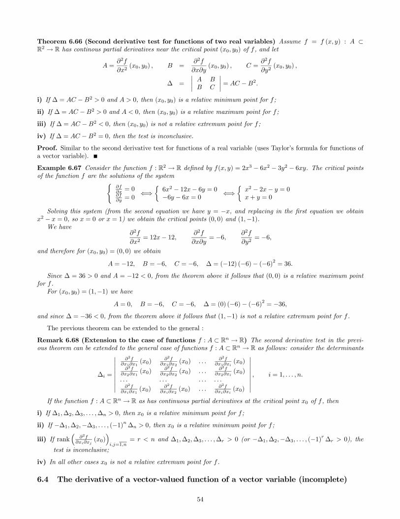
Theorem 6.66 (Second derivative test for functions of two real variables) Assume = ( ) : ⊂R2 → R has continous partial derivatives near the critical point (0 0) of , and let
=2
2(0 0) =
2
(0 0) =
2
2(0 0)
∆ =
¯̄̄̄
¯̄̄̄= −2
i) If ∆ = −2 0 and 0, then (0 0) is a relative minimum point for ;
ii) If ∆ = −2 0 and 0, then (0 0) is a relative maximum point for ;
iii) If ∆ = −2 0, then (0 0) is not a relative extremum point for ;
iv) If ∆ = −2 = 0, then the test is inconclusive.
Proof. Similar to the second derivative test for functions of a real variable (uses Taylor’s formula for functions of
a vector variable).
Example 6.67 Consider the function : R2 → R defined by ( ) = 23 − 62 − 32 − 6. The critical pointsof the function are the solutions of the system(
= 0
= 0
⇐⇒½62 − 12− 6 = 0−6 − 6 = 0 ⇐⇒
½2 − 2− = 0
+ = 0
Solving this system (from the second equation we have = −, and replacing in the first equation we obtain2 − = 0, so = 0 or = 1) we obtain the critical points (0 0) and (1−1).We have
2
2= 12− 12 2
= −6 2
2= −6
and therefore for (0 0) = (0 0) we obtain
= −12 = −6 = −6 ∆ = (−12) (−6)− (−6)2 = 36Since ∆ = 36 0 and = −12 0, from the theorem above it follows that (0 0) is a relative maximum point
for .
For (0 0) = (1−1) we have = 0 = −6 = −6 ∆ = (0) (−6)− (−6)2 = −36
and since ∆ = −36 0, from the theorem above it follows that (1−1) is not a relative extremum point for .
The previous theorem can be extended to the general :
Remark 6.68 (Extension to the case of functions : ⊂ R → R) The second derivative test in the previ-ous theorem can be extended to the general case of functions : ⊂ R → R as follows: consider the determinants
∆ =
¯̄̄̄¯̄̄̄¯
211
(0)2
12(0) 2
1(0)
221
(0)2
22(0) 2
2(0)
2
1(0)
22
(0) 2
(0)
¯̄̄̄¯̄̄̄¯ = 1
If the function : ⊂ R → R as has continuous partial derivatives at the critical point 0 of , then
i) If ∆1∆2∆3 ∆ 0, then 0 is a relative minimum point for ;
ii) If −∆1∆2−∆3 (−1)∆ 0, then 0 is a relative minimum point for ;
iii) If rank³
2
(0)´=1
= and ∆1∆2∆3 ∆ 0 (or −∆1∆2−∆3 (−1)∆ 0), the
test is inconclusive;
iv) In all other cases 0 is not a relative extremum point for .
6.4 The derivative of a vector-valued function of a vector variable (incomplete)
54
7 Exercises
1. Compute the the derivatives of the following functions at the indicated points using the definition:
(a) : [−1∞)→ R, () =√+ 1 at 0 = 3;
(b) : R→ R, () = cos at 0 = 3;
(c) : R→ R, () = ln¡1 + 2
¢at 0 = 1
2. Determine if the indicated functions are differentiable at the indicated points:
(a) : (−12∞)→ R, () =
½ln (1 + 2) ∈ ¡−1
2 0¢
2 ∈ [0∞) ;
(b) : (0∞)→ R, () =½ √
2 + + 2 ∈ (0 1)34+ 1
4 ∈ [1∞) ;
(c) : (0∞)→ R, () =½ √
2 + + 2 ∈ (0 1)34+ 5
4 ∈ [1∞) ;
3. Study the differentiability at 0 = 0 of the following functions:
(a) : R→ R, () =½sin 1
6= 0
0 = 0
(b) : R→ R, () =½
sin 1 6= 0
0 = 0
(c) : R→ R, () =½
sin 1 6= 0
0 = 0where ∈ N.
4. Compute the derivatives of the following functions:
(a) () = 43 − 52 + 7+ , () = sin+ cos¡2¢, () =
√2 + 1;
(b) () =¡2 + + 1
¢3, () = 3sin, () =
¡2 + + 1
¢sin;
(c) () = 2
, () =¡2 + 1
¢arcsin (), () =
3√2 + 1 ln (sin);
(d) () = 32+12++1
, () =ln(2+1)4+1
, () = tan2+cos
;
(e) () = sin(ln(2+1)), () = ln
¡sin¡2 + 1
¢+ 2¢, () = arcsin
¡sin2
¢.
5. Evaluate the following limits:
(a) lim→0 cos−12, lim→0 sin−3
, lim→0 tan−3
(b) lim→∞ 3
, lim→∞ ln
, lim→∞
( ∈ N, 0)
(c) lim→0ln(cos )
ln(cos ) lim&0
ln(sin )
ln(sin )( 0)
(d) lim→0¡1 + 1
¢, lim→0
µ(1+)
1
¶ 1
Hint: use L’Hôpital’s rule. In d) take logarithms and then compute the limit.
6. Compute the second order derivatives of the following functions:
(a) () = 4 − 52 + 7+ , () = sin+ cos (3), () = 2
(b) () = sin2 , () = tan, () = ln¡+√2 + 1
¢7. Compute the th order derivative of the following functions:
(a) () = ( ∈ R)(b) () = sin
55
(c) () = 1− ( ∈ R)
(d) () = 12−3+2
(e) () = ( 0)
8. Determine the extremum points of the following functions"
(a) : R→ R, () = 2 cos+ 2
(b) : R→ R, () = 2 (− 6)2
(c) : R→ R, () = 2 (− 6)4(d) : R→ R, () = 2 sin (2) + sin (4)
(e) : R→ R, () = 3
q(2 − 1)2
(f) : R→ R, () = 23 + 92 − 108+ 30(g) : R→ R, () = 23
(h) : [0 5]→ R, () = 23 − 32 − 36+ 2
9. Compute the indicated Taylor polynomials for the given function:
(a) () = 2 + 5+ 1, order = 3 at 0 = 0 and at 0 = 1;
(b) () = sin, order = 3 at 0 = 0;
(c) () = 2, order = 4 at 0 = 1;
(d) () = 1−1 , order = 4 at 0 = 2;
(e) () = ln (1− ), order = 3 at 0 = 0.
10. Use the tangent line approximation to approximate√10
Hint: consider the function : [0∞) given by () = √ and write the tangent line approximation for ()near the point = 9.
11. Use a Taylor polynomial of order 3 to approximate√10. Compare with the approximation obtained in the
previous exercise.
Hint: consider the function : [0∞) given by () = √ and write the approximation () ≈ 3 (), where
3 () is the Taylor polynomial of order 3 for () at the point 0 = 9.
12. Consider the function : R2 → R defined by (1 2) = 21 + 312 + 422.
(a) Show that is differentiable at (1 2) = (0 0) using the definition;
(b) Prove that is differentiable at (1 2) = (0 0) by using a theorem;
(c) Redo part a) and b) considering an arbitrary point¡01
02
¢.
13. Consider the function : R2 → R defined by
( ) =
½ 2+2
( ) 6= (0 0)0 ( ) = (0 0)
(a) Is continuous at ( ) = (0 0)?
(b) Is differentiable at ( ) = (0 0)?
(c) Does have partial derivatives at ( ) = (0 0)?
14. Consider the function : R2 → R defined by
(1 2) =
(31
21+22
(1 2) 6= (0 0)0 (1 2) = (0 0)
(a) Show that is continuous at (1 2) = (0 0);
56
(b) Compute 1
(0 0) and 2
(0 0)
15. Consider the function : R2 → R defined by
( ) =
(√2+2
( ) 6= (0 0)0 ( ) = (0 0)
Show that at the point (0 0) the function is continuous, has first order partial derivatives, but it is not
differentiable.
16. Show that the function : R2 → R defined by ( ) =p2 + 2 does not have partial derivatives at the
point (0 0). Is constinuous at (0 0)? Is differentiable at (0 0)?
17. Compute the following partial derivatives by using the definition:
(a) (1 1) and
(1 1), where ( ) = 3 − 2 + 3;
(b) (2 1) and
(2 1), where ( ) =
p2 − 2;
(c) (1 1) and
(1 1), where ( ) = −
+;
18. Compute the first order partial derivatives of the following functions:
(a) ( ) = 3 + 3 + 3 + 3;
(b) ( ) =p2 + 22 + 32;
(c) ( ) = arctg ;
(d) ( ) = ln³+
p2 + 2
´;
(e) ( ) = sin() ( 0 a constant);
(f) ( ) = arcsin³p
2 − ´.
19. Compute the second order partial derivatives of the following functions:
(a) ( ) = 3 + 3 + 3 + 3;
(b) ( ) = ln¡2 +
¢;
(c) ( ) = + + ;
20. Consider the function : R2 → R defined by (1 2) = 41 − 2312 − 12. Compute the indicated partial
derivatives:
(a) 1, 2;
(b) 2
21, 212
, 221
and 2
22;
(c) 3
31, 3121
, 3
122
and 3
212.
21. Consider the function : R2 → R defined by
(1 2) =
(12
21−2221+
22
(1 2) 6= (0 0)0 (1 2) = (0 0)
(a) Compute 1
and 2;
(b) Show that 212
(0 0) = 1 and 221
(0 0) = −1.
22. Consider a differentiable function = (1 2 3) : R3 → R.
(a) Compute the partial derivative(sin 2+tan +3)
;
57
(b) Verify your answer in b) using (1 2 3) = 21 + 32 − 33 by direct computation.
23. Consider a differentiable function = (1 2 3 4) : R4 → R.
(a) Compute the partial derivative(ln(+)−22+22+cos(+)−2)
;
(b) Compute the partial derivative(ln(+)−22+22+cos(+)−2)
;
(c) Compute the partial derivative(ln(+)−22+22+cos(+)−2)
;
(d) Compute the partial derivative(ln(+)−22+22+cos(+)−2)
;
(e) Verify your answers in a) — d) using (1 2 3 4) = 212 + 23 − 24 by direct computation.
24. Consider a differentiable function = (1 2 3) : R3 → R. Compute the indicated partial derivatives:
(a)(++−2+35−7+9)
,(++−2+35−7+9)
and
(++−2+35−7+9)
;
(b)(+sin 22+3+5)
,(+sin 22+3+5)
and
(+sin 22+3+5)
;
25. Consider the function : (0∞)×R→ R defined by ( ) = Compute the partial derivatives and .
26. Show that the function ( ) = ln¡2 + 2
¢defined on = R2 − {(0 0)} verifies the equation
∆ =2
2+
2
2= 0
(a function satisfying ∆ = 0 is called a harmonic function).
27. Show that the function (1 2 3 4) =1
21+22+
23+
24
defined on = R4−{(0 0 0 0)} verifies the equation
∆ =2
21+
2
22+
2
23+
2
24= 0
28. Consider a twice differentiable function : R→ R. Show that verifies the equation
2 (− )
2− 2 (− )
2= 0
Verify your answer by considering the function () = 2 = 3+ 5.
29. Show that the function ( ) = ln¡3 + 3 + 3 − 3¢ verifies the equation
+
+
=
1
+ +
30. Show that the function ( ) = ln¡2 + + 2
¢verifies the equation
+
= 2
31. Determine the indicated Taylor polynomials for the given functions:
(a) ( ) = sin (+ 2) + 2 + 4 + 3+ 5, order = 2 at the point (0 0)
(b) ( ) =p2 + 2, order = 2 at the point (1 3);
(c) ( ) = , order = 3 at the point (1 1);
(d) ( ) = +2, order = 3 at the point (0 0);
58
32. Determine the extremum points of the following functions:
(a) : R2→ R, ( ) = 3 + 32 − 15− 12;(b) : R2 → R, ( ) = 3 + 3 − 32 − 32 + 4;(c) : R2 → R, ( ) = 1
33 + 1
22 + 2 + 5+ ;
(d) : R2 → R, ( ) = 22 − 52 − 8 − 52;(e) : R2 → R, ( ) = (12− 3− 4)(f) : R2 → R, ( ) = 4 + 4 − 22 + 4 − 22
33. Find the critical points of the function : R4 → R defined by () = 21 + 22 + 23 − 24 − 212 + 413 +314 − 224 + 41 − 52 + 7
59
AppendixDerivatives of some common function
Function Derivative Domain
(constant) 0 ∈ R −1 ∈ R ( ∈ R∗ for 0)sin cos ∈ Rcos − sin ∈ Rtan 1
cos2 ∈ R−©2 ±
2: ∈ Zª
cot − 1sin2
∈ R− { : ∈ Z}arcsin 1√
1−2 ∈ (−1 1)arccos − 1√
1−2 ∈ (−1 1)arctan 1
1+2 ∈ R
arccot − 11+2
∈ R ∈ R ln ∈ Rln 1
0
Some basic differentiation properties
()0= 0 (− constant)
( + )0= 0 + 0
()0= 0 + 0µ
¶0=
0 − 0
2
=
·
(chain rule)
()0= · −1 · 0 + · 0 · ln
60