Embed Size (px)
Citation preview
Discussion Paper No. 856
DIFFERENCE OR RATIO:
IMPLICATION OF STATUS PREFERENCE ON STAGNATION
Yoshiyasu Ono Katsunori Yamada
October 2012
Revised March 2013 Secondly Revised January 2014
The Institute of Social and Economic Research Osaka University
6-1 Mihogaoka, Ibaraki, Osaka 567-0047, Japan
Difference or Ratio:
Implications of Status Preference on Stagnation*
by
Yoshiyasu Ono† and Katsunori Yamada‡
Abstract
We consider a dynamic macroeconomic model of households that regard relative
affluence as social status. The measure of relative affluence can be the ratio to, or the
difference from, the social average. The two specifications lead to quite different equilibrium
consequences: under the ratio specification full employment is necessarily realized, whereas
under the difference specification there is a case where a persistent shortage of aggregate
demand arises. Furthermore, using data of an affluence comparison experiment we
empirically find that the difference specification fits the data better than the ratio
specification. Therefore, affluence comparison can be a cause of persistent stagnation.
JEL classification: C91, E12, E24
Keywords: status, stagnation, unemployment.
* Permission by Masayuki Sato for usage of the data set originally used in Yamada and Sato (2013) is greatly
appreciated. We are indebted to helpful comments by Gerhard Illing and seminar participants in Ludwig-Maximillian’s University, Munich, and in the Economic and Social Research Institute, Cabinet Office, the Governemnt of Japan. This research is financially supported by a Grant-in-Aid for Scientific Research from the Japan Society for the Promotion of Science (JSPS).
†Institute of Social and Economic Research, Osaka University. Adress: 6-1 Mihogaoka, Ibaraki, Osaka 567-0047, Japan. E-mail: [email protected]
‡ Institute of Social and Economic Research, Osaka University. Adress: 6-1 Mihogaoka, Ibaraki, Osaka 567-0047, Japan. E-mail: [email protected]
1
1. Introduction
Recently many countries suffer from serious long-run recessions. One is the Great
Recession that spreads worldwide in the wake of the 2008 international financial crisis.
Another is Japan’s ‘lost decades’ that started when its asset bubble burst in 1990. Facing such
serious economic circumstances, economists now more than ever need an analytical
framework that can treat inefficient macroeconomic outcomes and valid policy options for
recovery from chronic stagnation.
The currently dominant research agenda for dealing with stagnation is the New
Keynesian approach promoted by researchers such as Christiano et al. (2005) and Blanchard
and Galí (2007). They considered microeconomic foundations of price sluggishness and
analyzed macroeconomic fluctuations. This type of analysis is quite successful in examining
short-run recessions that fade out as prices adjust. However, because it treats perturbations
around the full-employment steady state, in order to analyze chronic and serious stagnation
with unemployment we need a different theoretical framework. Along this line, in the recent
IMF annual conference Summers (2013) criticized too much reliance on the DSGE approach
in solving economic crises and emphasized the need for researchers to work on long-run
recessions rather than short-run business fluctuations. This paper shares the same view and
adopts a long-run stagnation model.
A long-run stagnation model in a dynamic optimization framework was first explored by
Ono (1994, 2001), following the spirit of Chapter 17 of Keynes’s General Theory.
Households in this model have an insatiable preference for money, which causes a liquidity
trap to appear. Prices continue to adjust, but nevertheless shortages of aggregate demand and
employment persist in the steady state. Murota and Ono (2011) also presented a model of
persistent stagnation in which status preference plays the same role in creating persistent
2
stagnation as does the insatiable preference for money. They considered three objects of
status preference—consumption, physical capital holding, and money holding—and found
that an economy grows or stagnates depending on which is the primary measure of status. If it
is money (an unproducible asset), persistent stagnation with unemployment occurs.
The above-mentioned insatiable desires for absolute and relative money holdings were
discussed by Keynes (1972, p. 326). He wrote: “Now it is true that the needs of human beings
may seem to be insatiable. But they fall into two classes—those needs which are absolute in
the sense that we feel them whatever the situation of our fellow human beings may be, and
those which are relative in the sense that we feel them only if their satisfaction lifts us above,
makes us feel superior to, our fellows.” It may, however, be ambiguous whether the target of
people’s desire is to hold money or wealth. In the literature of status preferences, such as
Corneo and Jeanne (1997) and Futagami and Shibata (1998), status concerns are often
defined with respect to wealth holdings.
Following this convention, we present a model with status preference for wealth, instead
of money holdings, and explore the possibility of persistent stagnation. In this analysis there
are two specifications of relative affluence. One is that people care about the difference of
their wealth holdings from the social average. The other is that people care about the ratio of
those to the social average.1 Murota and Ono assumed that people care about the difference
of money holdings because this specification was necessary for persistent stagnation to
occur. Corneo and Jeanne (1995) and Futagami and Shibata (1998) took the ratio as the
measure of status because that specification was required for endogenous growth to occur in
1 Clark and Oswald (1998) considered both the difference and ratio specifications of social status and
explored tax policy implications for both cases in a static setting.
3
their models.2 We examine both cases and find that persistent stagnation with unemployment
occurs under the difference specification but not under the ratio specification. Thus, if the
difference specification reflects the real world, our disequilibrium model offers a potential to
provide adequate policy implications for long-run stagnation.
We then empirically examine the two specifications to see which is more plausible. Data
are borrowed from the hypothetical discrete choice experiment of Yamada and Sato (2013).
They conducted a large-scale socially representative survey and estimated the effects of
income comparisons by applying the data to the random utility model framework of Train
(2009). While the framework is mostly used for parameter estimations of utility functions, as
in Viscusi et al. (2008), we instead conduct a horse race between the two specifications of
status preference and apply the Akaike Information Criteria (AIC) and R-squared to the
comparison. We find that the difference specification fits the data much better than the ratio
specification does, and hence the model that accommodates persistent stagnation is
supported.
Previous macroeconomic studies of the status preference, such as Cole et al. (1992),
Konrad (1992), Zou (1994), Corneo and Jeanne (1997) and Futagami and Shibata (1998),
investigated the effects of status preference on the economic growth rate. There are also
quantitative approaches that tested the validity of status preference, e.g. Abel (1990), Gali
(1994) and Bakshi and Chen (1996). They argued that observed asset price volatility can be
explained by the motivation to keep up with the Joneses. Our purpose is to relate status
preference to the possibility of persistent demand deficiency and long-run stagnation.
2 Under the difference specification and decreasing returns to real capital, Murota and Ono (2011) showed
that endogenous growth occurs when households regard real capital as status.
4
2. Two Specifications of Status Concern
We consider a representative household that cares about relative affluence, whose utility
is
, exp , (1)
where is the utility of consumption c, is the utility of money m for transactions,
, represents status preference, is total asset holdings, and is the social average of
. Functions and satisfy
0, 0, 0 ∞;
0, 0, 0 ∞, ∞ 0. (2)
Two types of status preference , are considered. One is that the household cares about
the difference (case D), and the other is that it cares about the ratio (case R).3
Case D: , , 0;
Case R: , , 0. (3)
The flow budget equation and the asset budget constraint are respectively
,
, (4)
where is the real interest rate, is the real wage, is the amount of employment, is
interest-bearing assets, is the nominal interest rate, and is a lump-sum tax. Obviously
satisfies
,
3 Quite different theoretical implications obtained from the ratio and difference specifications documented
below have nothing to do with so called the Keeping Up with the Joneses (KUJ) and the Running Away from the Joneses (RAJ) effects. While the utility function with the difference specification is always a KUJ type, the utility function with the ratio specification can be KUJ and RAJ, depending on the marginal rate of substitution.
5
where is the inflation rate. The number of representative households is normalized to unity
and each representative household owns one unit of labor endowment. Therefore, the amount
of employment x straightforwardly represents the employment rate.
Maximizing (1) subject to (4) gives a Ramsey equation and portfolio choice summarized
as
, ,
, (5)
where
= / ′ , , ,.
The transversality condition is
lim → 0. (6)
The firm sector is competitive and uses only labor with linear technology , where is
the labor productivity and is assumed to be constant. In this case, the firm sector infinitely
expands production if nominal commodity price is higher than / , but produces nothing
if is lower than / . Thus, with perfect flexibility of , takes the value that satisfies
, (7)
as long as a finite and positive amount of the commodity is traded. Since the profits in this
case are zero, the firm value equals zero. Therefore, interest-bearing assets b consist of only
government bonds.
In the money market,
,
where M is the nominal money stock. The monetary authority is assumed to keep M constant,
for simplicity, and thus
6
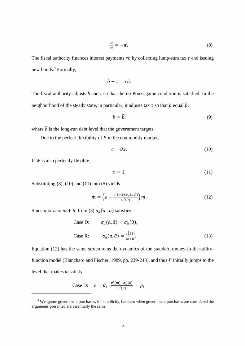
. (8)
The fiscal authority finances interest payments by collecting lump-sum tax and issuing
new bonds.4 Formally,
.
The fiscal authority adjusts and so that the no-Ponzi-game condition is satisfied. In the
neighborhood of the steady state, in particular, it adjusts tax so that equal :
, (9)
where is the long-run debt level that the government targets.
Due to the perfect flexibility of in the commodity market,
. (10)
If W is also perfectly flexible,
1. (11)
Substituting (8), (10) and (11) into (5) yields
,
. (12)
Since , from (3) , satisfies
Case D: , 0 ,
Case R: , . (13)
Equation (12) has the same structure as the dynamics of the standard money-in-the-utility-
function model (Blanchard and Fischer, 1989, pp. 239-243), and thus initially jumps to the
level that makes m satisfy
Case D: , ,
4 We ignore government purchases, for simplicity, but even when government purchases are considered the
arguments presented are essentially the same.
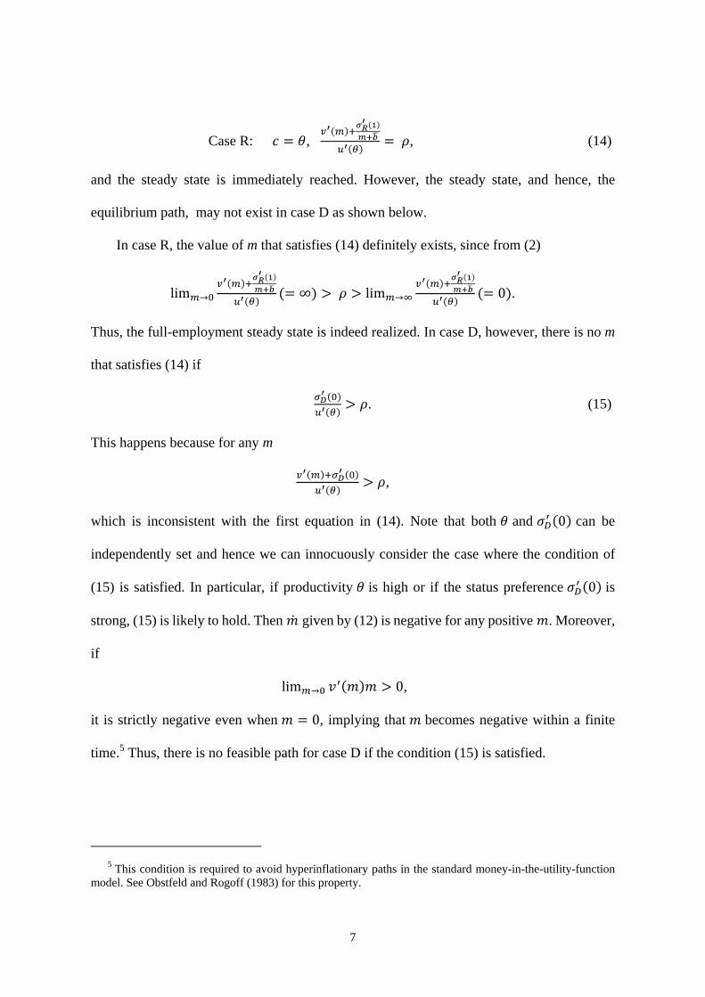
7
Case R: , , (14)
and the steady state is immediately reached. However, the steady state, and hence, the
equilibrium path, may not exist in case D as shown below.
In case R, the value of m that satisfies (14) definitely exists, since from (2)
lim → ∞ lim → 0 .
Thus, the full-employment steady state is indeed realized. In case D, however, there is no m
that satisfies (14) if
. (15)
This happens because for any m
,
which is inconsistent with the first equation in (14). Note that both and 0 can be
independently set and hence we can innocuously consider the case where the condition of
(15) is satisfied. In particular, if productivity is high or if the status preference 0 is
strong, (15) is likely to hold. Then given by (12) is negative for any positive . Moreover,
if
lim → 0,
it is strictly negative even when 0, implying that becomes negative within a finite
time.5 Thus, there is no feasible path for case D if the condition (15) is satisfied.
5 This condition is required to avoid hyperinflationary paths in the standard money-in-the-utility-function
model. See Obstfeld and Rogoff (1983) for this property.
8
3. Persistent Stagnation under the Difference Specification
In the previous section, we find that under the difference specification (case D) and
flexible adjustments of and there is no dynamic equilibrium path if (15) holds. This is
because preference for money holding always dominates preference for consumption. This
would naturally suggest a shortage of aggregate demand although it is not allowed to exist
due to the assumption of perfect flexibilities of prices and wages. Therefore, we introduce
sluggish wage adjustments to the model so as to allow for a shortage of aggregate demand.
Consequently, we find that the dynamic equilibrium path exists and that shortages of
aggregate demand and employment remain even in the steady state.6
Recent dominant settings of wage adjustments are the New Classical, the New
Keynesian, and the hybrid Phillips curves. They well fit to analyze short-run fluctuations
around the full-employment steady state, but not to examine persistent stagnation because
they are set up so that the inflation-deflation rate cumulatively expands as long as market
disequilibrium exists.7 Thus, the possibility of unemployment in a steady state, which we
focus on, is intrinsically eliminated. In order for the unemployment steady state to be
possible, we adopt the conventional Walrasian wage adjustment process:
1 , (16)
where is the adjustment speed. Obviously, this is a simplified form of wage adjustment
without a microeconomic foundation but we can provide a microeconomic foundation for
this type of adjustment. In the appendix we indeed apply the wage adjustment mechanism
with a microeconomic foundation proposed by Ono and Ishida (2013) to the present model
6 Obviously, nominal wage sluggishness does not exclude the case where full employment is reached in the
steady state. 7 See Woodford (2003) for properties of those Phillips curves.
9
and show that the same steady state with the same stability property as presented below
obtains.
Because always moves in proportion to , as shown by (7), the wage adjustment
mechanism (16) leads to
1 .
From (4), (5), (8), (9), (10) and the above equation, we obtain an autonomous dynamic
system:
, 1 ,
1 ,
. (17)
where , is given by (13). The full-employment steady state given by (14) is
eventually reached as long as it exists.8 It always is the case in case R, and also in case D with
(15) being invalid.
However, if (15) holds in case D, a steady state with full employment given by (14) does
not exist. Then, the first and second equations of (17) form a two-dimensional autonomous
dynamic system with respect to and :
1 ,
1 . (18)
Because is sluggish, initially takes the value that satisfies (7) for the initial . Then
determines the initial level of , while jumps to the amount that is on the saddle path.9
Along this path, a demand shortage remains and deflation continues.
8 The uniqueness and the stability of the present dynamics are proved in the same way as in Ono (1994, 2001), who treats the case where b = 0.
10
In the steady state of the present dynamics, from (18) satisfies
Φ ≡ 1 0. (19)
From (15), one has
Φ 0. (20)
Therefore, for (19) to have a positive solution, it must be valid that
Φ 0 0, (21)
and then satisfies
0 ,
which implies a persistent demand shortage. Deflation continues, making m diverge to
infinity. Nevertheless, the transversality condition (6) is valid since
lim → ,
and . Note that in this state 0 and thus the second equation of (5) yields
0,
i.e., the zero interest rate holds.
Let us mention the economic implication of the difference between the two relative
affluence specifications. In case R, in which households care about the ratio of their asset
holdings to the social average, the marginal utility of real money balances, represented by
′ 1 ⁄ , converges to zero as approaches infinity. Thus, there is a level
of that equalizes the desire to accumulate real money balances to the desire to consume
sufficient commodities to realize full employment, and then the steady state with full
9 The dynamic equations given in (18) are mathematically the same as those in the case where there is a
strictly positive upper bound on the marginal utility of money, as analyzed by Ono (2001). He showed that there is a unique dynamic path and that it converges to the stagnation steady state if (15) is valid.
11
employment obtains. In case D, in which households care about the difference, the desire to
accumulate assets 0 remains strictly positive. Thus, if (15) holds, no matter how much
assets the households accumulate, the desire to accumulate money as an asset stays to be
higher than the desire to consume sufficient commodities to realize full employment. A
demand shortage remains despite continued declining prices and expanding real balances.
4. Experimental Evidence of the Two Specifications of Status
In the previous section we showed that persistent stagnation arises as an equilibrium
outcome when households care about not the ratio of their asset holdings to, but the
difference from, the social average. To see relevance to the real world, we investigate which
of the two specifications of relative affluence is more plausible.
We use the data set created by the hypothetical discrete choice experiment of Yamada
and Sato (2013), which includes 48,172 observations from 10,203 respondents. They
conducted an original Internet-based survey in February 2010 with Japanese subjects, and
investigated the intensity and sign of income comparisons against the social average.10 By
applying the data to a random utility model framework, they estimated the following utility
function with relative affluence:11
, , (22)
where y is the subject’s income and is the social average of income. We replace (22) by the
two utility specifications with a single composite variable given in (3), so that we can focus
10 By setting up an experiment such that parameters were fully randomized and choice situations were
orthogonal, they exploited full potential of the discrete choice experiment framework to find if the subjects had altruism or jealousy. See section 3 of Yamada and Sato (2013) for details of the experimental setting. Experimental details are provided in a supplemental material of this paper.
11 This setting was first presented by Dupor and Liu (2003) and Liu and Turnovsky (2005).
12
on a comparison of the two. We then apply the conditional logit model framework and
compare their AICs to see which specification better fits the data.
Note that there is a gap between the theoretical structure in the previous sections and the
experimental setting given below. In the choice experiment of Yamada and Sato (2013), the
relative affluence is associated with income, whereas in our model it is with asset holdings.
That said, income is a predictor of asset holdings under the permanent income hypothesis.
Moreover, Headey and Wooden (2004) found that income and asset holdings are both
important determinants of subjective well-being, and that the positive effect of asset holdings
on subjective well-being is taken away when adding an income term as an additional control.
This evidence suggests that income is a good proxy for asset holdings in the happiness
analyses. Therefore, we take income y as a proxy for assets a and replace , given in (3)
by , .
To facilitate the experimental data of Yamada and Sato (2013) to conduct a horse race of
the ratio and difference specifications, let us reformulate the model to the following random
utility model:
, ,
where represents each income scenario, is
Case D: ,
Case R: ,
is the marginal utility from the status, is the constant term, and ϵ is the error term that
follows an independent and identical distribution of extreme value type 1 (IIDEV1). The
probability that respondents prefer income situation to income situation is given by
Prob , , , forall .
13
By assuming IIDEV1 for the error term we consider a conditional logit model (McFadden,
1974) and estimate the parameter of the random utility function using the maximized
likelihood method. We also assume that irrelevant alternatives are independent (IIA), and
that the random components of each alternative and those within each subject are
respectively uncorrelated.
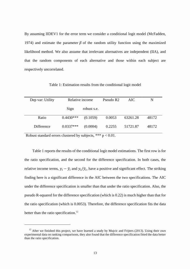
Table 1: Estimation results from the conditional logit model
Dep var: Utility Relative income Pseudo R2 AIC N
Sign robust s.e.
Ratio 0.4430*** (0.1059) 0.0053 63261.28 48172
Difference 0.0337*** (0.0004) 0.2255 51721.87 48172
Robust standard errors clustered by subjects, *** p < 0.01.
Table 1 reports the results of the conditional logit model estimations. The first row is for
the ratio specification, and the second for the difference specification. In both cases, the
relative income terms, and / , have a positive and significant effect. The striking
finding here is a significant difference in the AIC between the two specifications. The AIC
under the difference specification is smaller than that under the ratio specification. Also, the
pseudo R-squared for the difference specification (which is 0.22) is much higher than that for
the ratio specification (which is 0.0053). Therefore, the difference specification fits the data
better than the ratio specification.12
12 After we finished this project, we have learned a study by Mujcic and Frijters (2013). Using their own
experimental data on ranking comparisons, they also found that the difference specification fitted the data better than the ratio specification.
14
In section 3 we have found that with the difference specification persistent stagnation
can occur while with the ratio specification full employment is always reached in the steady
state. Because the present experimental result supports the former, we may conclude that our
model accommodates persistent stagnation and unemployment.
5. Conclusion
When relative affluence compared to the social average is taken as status, the measure
can be the ratio to, or the difference from, the social average. The two specifications lead to
mutually quite different scenarios of business activity. If it is the ratio, full employment is
necessarily reached in the steady state. If it is the difference, there is a case where
unemployment and stagnation due to shortage of aggregate demand appear in the steady
state. This case arises particularly if the output capacity is high or if the desire for the relative
affluence is strong.
Using the experimental data on income comparison carried out by Yamada and Sato
(2013), we find that the difference specification fits the data better than the ratio specification
does. Therefore, relative affluence can be a cause of persistent stagnation, and our model can
be a good platform to analyze persistent stagnation. Furthermore, since the mathematical
structure of the present model is essentially the same as that of Ono (1994, 2001), the same
policy implications as those of Ono hold. They are quite different from those under the
conventional models and are more in conformity with classical wisdom of Keynes (1936): an
increase in government purchases expands private consumption, while improvements in
productivity and wage adjustments reduce private consumption and worsen stagnation.
15
Appendix: Stability with a microeconomic foundation of sluggish wage adjustment
In the text we assume the conventional Walrasian wage adjustment process that lacks a
microeconomic foundation, represented by (16). Ono and Ishida (2013) extended the
fair-wage hypothesis a la Akerlof (1982) and Akerlof and Yellen (1990) to a dynamic setting
and proposed a microeconomic foundation of wage adjustment that converges to the
conventional Walrasian one. Furthermore, they applied it to a money-in-the-utility-function
model and obtained the condition that makes the stability and uniqueness of the steady state
hold. This appendix introduces that wage adjustment mechanism, instead of (16), to the
present model and shows that under conditions (20) and (21) the unemployment steady state
given by (19) is reached.
Let us start the analysis by summarizing the dynamics of fair wages presented by Ono
and Ishida (2013). Employed workers randomly separate from the current job at the Poison
rate , and therefore total employment , which also represents the employment rate because
the population is normalized to unity, changes in the following way:
, (A1)
where is the number of workers that are newly hired. While workers are employed, they
form fair wage in mind by referring to their past wages, their fellow workers’ fair wages
(which equal their own) and the unemployment situation of the society. More precisely, they
first consider the rightful wage , which is the wage that they believe fair if everybody is
employed. Therefore, ∆ , implying the rightful wage that is ex post conceived at time
∆ , is calculated so that the current fair wage equals the average of ∆ and the
zero income of the unemployed. Because the number of the employed is ∆ , it
satisfies
∆ ∆ ∆ . (A2)
16
Newly hired workers, in contrast, do not have any preconception about the fair wage and
simply follow the incumbent workers’ conceptions.
At time the number of new comers is ∆ . Therefore, when the incumbent workers
calculate the fair wage , the total number of workers that they care is 1 ∆ .
Because the rightful wage that they have in mind is the one that was ex post conceived at time
∆ , which is ∆ in (A2), and the number of the incumbent workers is
∆ 1 ∆ , is formed as follows:
∆ ∆ ∆
∆.
Substituting (A2) into the above equation and rearranging the result leads to
∆
∆∆ .
Therefore, by reducing ∆ to zero we obtain
. (A3)
The representative firm is competitive and takes commodity price as given. In the
presence of unemployment, it will set the wage equal to the fair wage because the fair wage is
the lowest wage under which the employees properly work. The commodity price adjusts to
⁄ since there is no commodity supply if ⁄ and excess commodity supply if
⁄ . Under full employment the firm tries to pick out workers from rival firms to
expand the market share by raising the wage so long as the marginal profits are positive,
making equal to .
Note that follows the movement of the fair wage in the presence of unemployment and
that follows the movement of in the absence of unemployment. Thus, anyway we have
,
which yields
17
. (A4)
From (5), the time differentiation of (10), (A1), (A3) and (A4), in the presence of
unemployment we obtain an autonomous dynamic system of and .
, ≡ / , 1 ,
, ≡ / , 1 , (A5)
instead of (17). Note that in the neighborhood of the steady state, where 0, in (A5)
equals
1 ,
as is the case in the dynamics given by (17). This is the Walrasian adjustment in which
adjustment speed is the Poison rate of job separation or equivalently 1/ is the average
duration of employment. The steady state condition of the first dynamic equation of (A5) is
equivalent to (19) and then a shortage of aggregate demand persists. In this steady state, from
(5) and (8) we find
, 0.
Therefore,
lim → exp 0,
i.e., deflation continues and nevertheless the transversality condition is valid.
Let us next examine the dynamic stability. The characteristic equation of the dynamics
given by (A5) is
0. (A6)
The partial derivatives of and are obtained from (A5) as follows:
/
,
18
/
,
/
,
/
.
in the neighborhood of the state in which 0. Therefore,
/
/
, (A7)
where
0 in case D,
in case R. (A8)
If full employment is achieved in the steady state, and 0 and then from (A7)
and (A8),
1/
0. (A9)
If unemployment continues in the steady state, which occurs only in case D, from (13) we
find
0. (A10)
From (20) and (21) Φ satisfies
Φ 0. (A11)
Therefore, if
lim → 0,
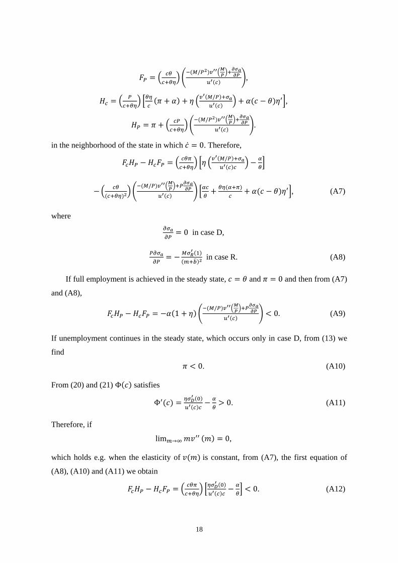
which holds e.g. when the elasticity of is constant, from (A7), the first equation of
(A8), (A10) and (A11) we obtain
0. (A12)
19
From (A9) and (A12), in either case one of the two solutions of (A6) is positive and the other
is negative. Note that in the presence of unemployment follows the movement of , which
cannot jump, as mentioned below equation (A3). Because is jumpable while is not, the
dynamics is saddle-path stable.
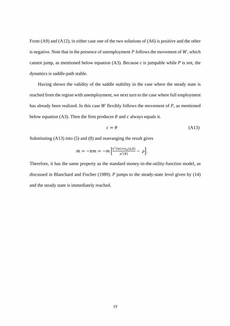
Having shown the validity of the saddle stability in the case where the steady state is
reached from the region with unemployment, we next turn to the case where full employment
has already been realized. In this case flexibly follows the movement of , as mentioned
below equation (A3). Then the firm produces and always equals it.
(A13)
Substituting (A13) into (5) and (8) and rearranging the result gives
, .
Therefore, it has the same property as the standard money-in-the-utility-function model, as
discussed in Blanchard and Fischer (1989). jumps to the steady-state level given by (14)
and the steady state is immediately reached.
20
References
Abel, A. B. (1990) “Asset prices under habit formation and catching up with the Joneses,”
American Economic Review, Vol. 80, pp. 43–47.
Akerlof, G. A. (1982) “Labor contracts as partial gift exchange,” Quarterly Journal of
Economics, Vol. 97, pp. 543–569.
Akerlof, G. A., and J. L. Yellen (1990) “The fair-wage effort hypothesis and
unemployment,” Quarterly Journal of Economics, Vol. 105, pp. 255–284.
Bakshi, G.S., and Z. Chen (1996) “The spirit of capitalism and stock-market prices,”
American Economic Review Vol. 86, pp. 133–157.
Blanchard Olivier J., and Stanley Fischer (1989) Lectures on Macroeconomics, Cambridge,
MA: MIT Press.
Blanchard, Olivier J., and Jordi Galí (2007) “Real wage rigidities and the new Keynesian
model,” Journal of Money, Credit and Banking, Vol. 39, pp. 35–65.
Christiano, Lawrence, Martin Eichenbaum and Charles Evans (2005) “Nominal rigidities
and the dynamic effects of a shock to monetary policy,” Journal of Political Economy,
Vol. 113, pp. 1-45.
Clark, Andrew E., and Andrew J. Oswald (1998) “Comparison-concave utility and following
behaviour in social and economic settings,” Journal of Public Economics, Vol. 70, pp.
133-155.
Cole, L.H., G.J. Mailath and A. Postlewaite (1992) “Social norms, savings behavior, and
growth,” Journal of Political Economy, Vol. 100, pp. 1092–1125.
Corneo, Giacomo, and Olivier Jeanne (1997) “On relative wealth effects and the optimality
of growth,” Economics Letters, Vol. 54, pp. 87-92.
21
Dupor, Bill, and Wen-Fang Liu (2003) “Jealousy and equilibrium overconsumption,”
American Economic Review, Vol. 93, pp. 423–428.
Futagami, Koichi, and Akihisa Shibata (1998) “Keeping one step ahead of the Joneses:
status, the distribution of wealth, and long run growth,” Journal of Economic Behavior
and Organization, Vol. 36, pp. 109-126.
Gali, J. (1994) “Keeping up with the Joneses: consumption externalities, portfolio choice and
asset prices,” Journal of Money, Credit and Banking, Vol. 26, No. 1–8.
Headey, Bruce, and Mark Wooden (2004) “The effects of wealth and income on subjective
well-being and ill-being,” Melbourne Institute Working Paper Series wp2004n03,
Melbourne Institute of Applied Economic and Social Research, The University of
Melbourne.
Keynes, John M. (1972) “Economic possibilities for our grandchildren,” in Essays in
Persuasion, The Collected Writings of John Maynard Keynes, Vol. IX, London:
Macmillan, pp. 321-332. Originally published in 1930.
Keynes, John M. (1936) The General Theory of Employment, Interest and Money, London:
Macmillan.
Konrad, K. (1992) “Wealth seeking reconsidered,” Journal of Economic Behavior and
Organization, Vol. 18, pp. 215–227.
Liu, Wen-Fang, and Stephen J. Turnovsky (2005) “Consumption externalities, production
externalities, and long-run macroeconomic efficiency,” Journal of Public Economics,
Vol. 89, pp. 1097–1129.
McFadden, Daniel (1974) “Conditional logit analysis of qualitative choice behavior,” in Paul
Zarembka, ed., Frontiers in Econometrics, New York: Academic Press.
Mujcic, Redzo, and Paul Frijters (2013) “Economic choices and status: measuring
22
preferences for income rank,” Oxford Economic Papers, Vol. 65, pp. 47-73.
Murota, Ryuichiro, and Yoshiyasu Ono (2011) “Growth, stagnation and status preference,”
Metroeconomica, Vol. 62, pp. 112-149.
Obstfeld, Maurice, and Kenneth Rogoff (1983) “Speculative hyperinflations in
macroeconomic models: can werule them out?,” Journal of Political Economy, Vol.
91, pp. 675-687.
Ono, Yoshiyasu (1994) Money, Interest, and Stagnation - Dynamic Theory and Keynes's
Economics, Oxford University Press.
Ono, Yoshiyasu (2001) “A reinterpretation of chapter 17 of Keynes’s General Theory:
effective demand shortage under dynamic optimization,” International Economic
Review, Vol. 42, pp. 207-236.
Ono, Yoshiyasu, and Junichiro Ishida (2013) “On persistent demand shortages: a behavioral
approach,” Japanese Economic Review, forthcoming, published online, doi:10.1111/
jere.12016.
Summers, L. (2013) “14th Annual IMF Research Conference: Crises Yesterday and Today,
Nov. 8, 2013” available at http://www.youtube.com/watch?v=KYpVzBbQIX0
Train, Kenneth E. (2009) Discrete Choice Methods with Simulation, 2nd edition, Cambridge:
Cambridge University Press.
Viscusi, W. K., J. Huber and J. Bell (2008) “Estimating discount rates for environmental
quality from utility-based choice experiments,” Journal of Risk and Uncertainty, Vol.
37, pp. 199–220.
Woodford, Michael (2003) Interest and Prices, Princeton: Princeton University Press.
Yamada, Katsunori, and Masayuki Sato (2013) “Another avenue for anatomy of income
comparisons: evidence from hypothetical choice experiments,” Journal of Economic
23
Behavior and Organization, Vol. 89, pp. 35-57.
Zou, H.F. (1994) “The spirit of capitalism and long run growth,” European Journal of
Political Economy, Vol. 10, pp. 279–293.


![Basel 3 & Implication[1]](https://img.pdfslide.us/doc/110x75/577d1e721a28ab4e1e8e9042/basel-3-implication1.jpg)