Embed Size (px)
Citation preview

WM2 ‐ Bioinformatics
ExomeSeq data analysis
Dietmar Rieder

Ul%mate goal is to iden%fy soma%c varia%on in sequencing data
RAW READS SEQUENCE DATA
GENOMIC VARIATION
processing + analysis

Bedrock of soma%c variant discovery: T/N pair comparisons
TUMOR
NORM
AL

Types of variants
Meyerson, Gabriel and Getz. Nat. Rev. Genet. (2010)

Typical number of soma%c muta%ons
1000s to 10,000s soma%c single nucleo%de varia%ons (sSNVs) 100s to 1,000s soma%c small inser%ons and dele%ons (sINDELs) 100s to 1,000s soma%c structural varia%ons (sSVs) 100s to 1,000s soma%c copy number altera%ons (sCNAs)
Spectral karyotypes (SKY)
In a genome of 3 x 10⁹ bases:
h[p://www.path.cam.ac.uk/~pawefish/BreastCellLineDescrip%ons/HCC1954.html
Cancer Cell Normal Cell

Types of variants
Meyerson, Gabriel and Getz. Nat. Rev. Genet. (2010)

Remember T/N pair comparisons
TUMOR
NORM
AL

Two main types of false posi%ves TU
MOR
NORM
AL
1. NO EVENT, JUST NOISE
At risk: Every base Source: Misread bases Sequencing ar%facts Misaligned reads
At risk: ~1000 germline / Mb (known) Source: Low coverage in normal
TUMOR
NORM
AL
2. GERMLINE EVENT (in T+N)
FPTotal = FPNoEvent + FPGermline

Addi%onal source of false nega%ves: “Tumor in Normal”
TUMOR
NORM
AL
• Due to contamina%on of the normal sample by tumor cells • Appears to be a germline event and leads to rejec%on of real variant

Now, throw in the variant allelic frac%on problem
N T
T
The (variant) allelic frac%on is the frac%on of alleles (DNA molecules) from a locus that carry the variant -‐> Also the expected frac%on of suppor%ng reads
33% N 67% T
(1) Purity = 67% (2) Local copy number in tumor = 4 (3) Number of mutated copies per cancer cell = 1 -‐> Allelic frac%on = 2/10 = 0.2
Carter et al. Nat. Biotechnol. (2012)
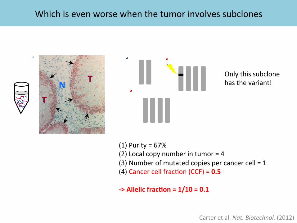
Which is even worse when the tumor involves subclones
N T
T
Carter et al. Nat. Biotechnol. (2012)
(1) Purity = 67% (2) Local copy number in tumor = 4 (3) Number of mutated copies per cancer cell = 1 (4) Cancer cell frac%on (CCF) = 0.5 -‐> Allelic frac%on = 1/10 = 0.1
Only this subclone has the variant!

Discovering low-‐frac%on variants requires deeper sequencing
©20
13 N
atur
e A
mer
ica,
Inc.
All
righ
ts r
eser
ved.
NATURE BIOTECHNOLOGY ADVANCE ONLINE PUBLICATION 3
A N A LY S I S
The LOD score is useful as a threshold for detection, as observed in the concordance of predicted sensitivity and measured sensitivity from the virtual-tumor approach (Fig. 2). Nonetheless, the LOD score cannot be immediately translated into the probability that a variant is due to true mutation rather than to sequencing error because the LOD score is calculated under an assumption of independent sequenc-ing errors and accurate read placement. As we discuss below, these assumptions are incorrect, and as a result, although direct applica-tion of the LOD score accurately estimates the sensitivity to detect a mutation, it substantially underestimates the false positive rate.
Variant filteringTo eliminate these additional false positives due to inaccurate read placement and non-independent sequencing errors, we developed six filters (Fig. 1 and Table 1). In addition, we used a panel of normal samples as controls to eliminate both germ-line events and artifacts (Online Methods). Subsets of these filters define several versions of the method (Fig. 1): (i) standard (STD), which applies no filters and thus includes all detected variants; (ii) high-confidence (HC), which applies the six filters and (iii) high-confidence plus panel of normal samples (HC + PON), which additionally applies the ‘panel of normal samples’ (PON) filter.
We tested the utility of these filters by applying them to the virtual-tumors benchmark and recomparing the results with the calculations (Fig. 2a). The sensitivity estimated for both with (HC) and with-out (STD) filters was similar, indicating that the model is accurate with respect to detection and that the filters do not adversely impact sensitivity. However, after applying the filters (HC), specificity increased and closely followed the calculations, suggesting that the filters largely eliminate systematic false positives (Fig. 2a and Supplementary Fig. 3).
Variant classificationFinally, each variant detected in the tumor sample is designated as somatic (not present in the matched normal sample), germ-line (present in the matched normal sample) or variant (present in the tumor sample but indeterminate status in the matched normal sample as a result of insufficient data). To perform this classification, we used a LOD score that compares the likelihood of the data under models in which the variant is present as a heterozygote or absent in the matched normal sample (Online Methods). We declare that there are
insufficient data for classification if the power to make a germ-line classification is less than 95%. We also used public germ-line variation databases41 as a prior probability of an event being germ-line.
SensitivityWe applied several benchmarking methods to evaluate the sensitiv-ity of our method to detect mutations as a function of sequencing depth and allelic fraction (Fig. 2b). First, we calculated the sensitivity under a model of independent sequencing errors and accurate read placement using our statistical test given an allelic fraction and tumor sample sequencing depth, and assuming that all bases have a fixed base quality score of Q35 (approximate mean base quality score in simulation data; Online Methods and Supplementary Fig. 4).
Next, to apply the downsampling benchmark, we used 3,753 validated somatic mutations, stratified by allele fraction (median = 0.28, range = 0.07–0.94), in colorectal cancer7 with deep-coverage ( 100×), exome-capture sequencing data downloaded from the data-base of Genotypes and Phenotypes (dbGAP; phs000178). Finally, to apply the virtual-tumor benchmark, we used deep-coverage data from two high-coverage, whole-genome samples (Coriell individ-uals NA12878 and NA12981) sequenced on Illumina HiSeq instru-ments as part of the 1000 Genomes Project42 and another previous study43, across 1 Gb of genomic territory. Note that we cannot use the PON filter (HC + PON) in the virtual-tumor sensitivity benchmark because it discards common germ-line sites.
Sensitivity estimates based on these three approaches were highly consistent with each other (median coefficients of variation for each depth of 3.1%). This suggests that the benchmarking approaches accu-rately estimate the sensitivity of mutation-calling methods and also that the calculated sensitivity is robust across a large range of para-meter values, enabling us to confidently extrapolate to higher sequenc-ing depths and lower allele fractions (Supplementary Table 1).
Based on this analysis, we observed that MuTect is a highly sensitive detection method. It detected mutations at a site with 30× depth in the tumor data (typical of whole-genome sequencing) and an allele frac-tion of 0.2 with 95.6% sensitivity. The sensitivity increased to 99.9% with deeper sequencing (50×) and dropped to 58.9% for detecting mutations with allelic fraction of 0.1 (at 30× sequencing; Fig. 2b and Supplementary Table 1). With 150× sequencing depth (typical of exome sequencing) we observed 66.4% sensitivity for 3% allele frac-tion events. It is this sensitivity to detect low-allele-fraction events
0 10 20 30 40 50
0
0.2
0.4
0.6
0.8
1.0
False positive rate (Mb–1)
Sen
sitiv
ity
a
0 5 10 15 20
0.85
0.90
0.95
1.00
6.36.3
6.3
Calculation (Q35)
MuTect STD
MuTect HC
0 10 20 30 40 50 60
0
0.2
0.4
0.6
0.8
1.0
Tumor sample sequencing depth
Sen
sitiv
ity
b
Calculation (Q35) f = 0.4
f = 0.2
f = 0.2
f = 0.1
f = 0.05
•
••
•6.36.3
6.3••
MuTect STD (virtual tumors)
MuTect HC (virtual tumors)
MuTect HC + PON (downsampling)
MuTect HC (downsampling)
Figure 2 Sensitivity as a function of sequencing depth and allelic fraction. (a) Sensitivity and specificity of MuTect for mutations with an allele fraction of 0.2, tumor sample sequencing depth of 30× and normal sample sequencing depth of 30× using various values of the LOD threshold ( T) (0.1 T 100). Calculated sensitivity and false positive rate using a model of independent sequencing errors with uniform Q35 base quality scores and accurate read placement (Calculation) are shown as well as results from the virtual-tumor approach for the standard (MuTect STD) and high-confidence (MuTect HC) configurations. A typical setting of T = 6.3 is marked with black circles. (b) Sensitivity as a function of tumor sample sequencing depth and allele fraction (f ) using T = 6.3. Calculated sensitivity as in a is shown
as well as results from the virtual-tumor approach and the downsampling of validated colorectal mutations7. Error bars, 95% confidence intervals (typically smaller than marks).
Sensi%vity (recall) decreases with the variant allele frac%on
Cibulskis et al. Nat. Biotechnol (2013)
AF=0.4
AF=0.2
AF=0.1
AF=0.05
For MuTect

Soma%c Variant Discovery Workflow
Indels adz¢ŜŎǘн
+ some post-‐processing to rescue TiN variants and eliminate ar%facts
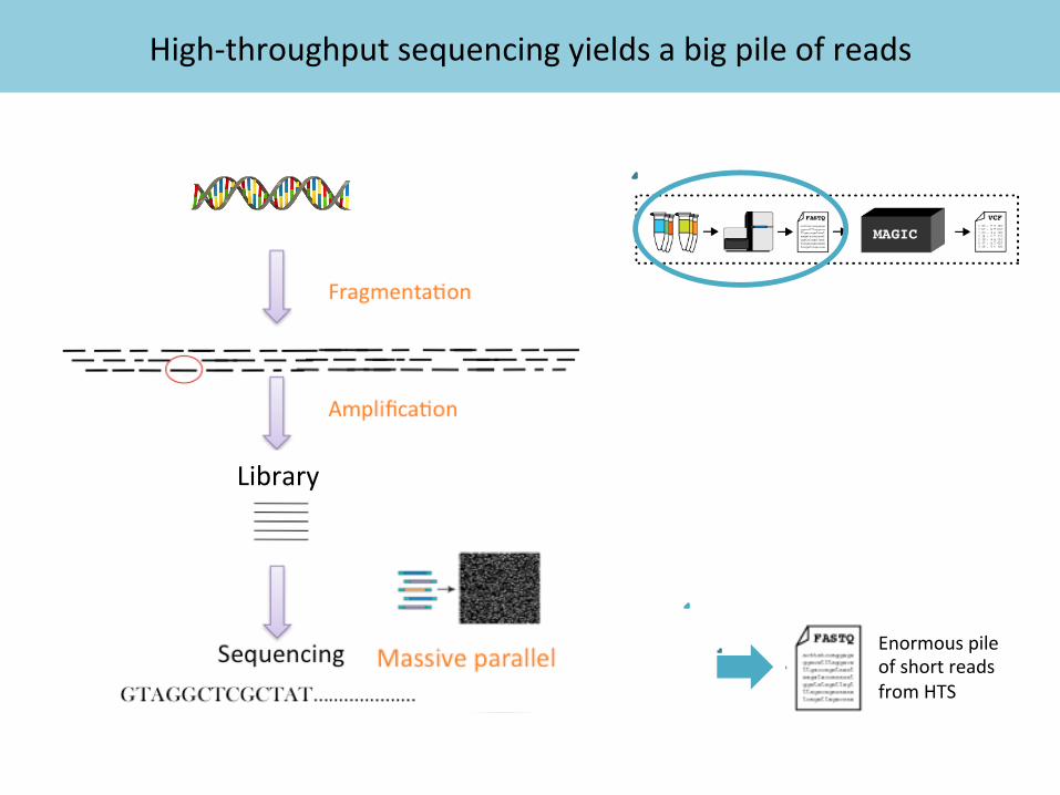
High-‐throughput sequencing yields a big pile of reads
Enormous pile of short reads from HTS
Library

Instruments generate short reads that must be mapped to the reference
Enormous pile of short reads from HTS
Reference genome
Mapping and alignment algorithms
Reads mapped to reference

How we visualize aligned HTS reads (Integrated Genomics Viewer)
Depth of coverage
Individual reads aligned to the genome
Clean C/T heterozygote
First and second read from the same fragment
Reference genome
Non-‐reference bases are colored; reference bases are grey

Intergenic Exon I Exon IIIntron I IntergenicVariant site
Small targeted experiments, gene panels, RADseq • Similar to exomes for most purposes
Whole genome
Exome
Whole genome (WGS) vs. Exome (WEx)

Key differences between whole genome and exome
Whole genome • En)re genome is prepped • Possible to do PCR-‐free • Higher price • Exons + introns • Coverage everywhere
(well, almost – some missing)
Exome • Capture of target regions • PCR required • Lower price • Exons only • Coverage only on targets
(well, almost – some spillover)

Key differences between whole genome and exome
0
10
20
30
40
50
60
70
80
90
100
10X 20X 30X 40X 50X 100X
Percen
t of b
ases at coverage de
pth
Base coverage depth
Typical Sample Metrics
WES
WGS
• To achieve 80% at 20X target for exomes, many bases are covered up to 100X
• WGS achieves mean coverage >20X with fewer high coverage bases
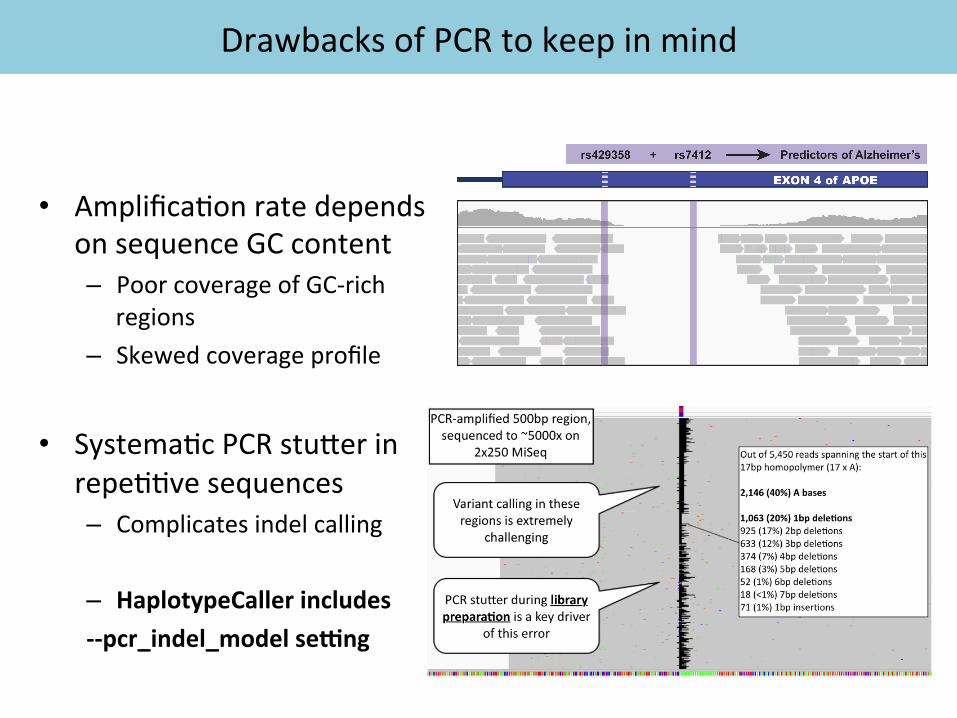
Drawbacks of PCR to keep in mind
• Amplifica)on rate depends on sequence GC content – Poor coverage of GC-‐rich
regions – Skewed coverage profile
• Systema)c PCR stuker in
repe))ve sequences – Complicates indel calling
– HaplotypeCaller includes -‐-‐pcr_indel_model seWng

Exome capture target regions
• Involves baits (complementary sequences) )led to capture segments of target regions
Broad uses a custom-‐designed bait set; the target intervals list is available in our resource bundle
(Clark et al, Nat. Biotech., 2011)
• Resul)ng covered intervals are specific to capture kit manufacturer
(Clark et al, Nat. Biotech., 2011)

Effect on ability to compare datasets
• If samples were sequenced by different centers, with different capture or enrichment kits, covered (strictly usable) intervals are not equivalent.
• Must decide whether to use union or intersec)on of interval lists (we use intersec)on)
common intervals
A B

What about gene panels?
• Targeted gene panels – Func)onally similar to exome
with very small interval list (e.g. 200)
o Same drawbacks as exomes PLUS some new ones
o Produces many independent fragments with iden)cal start and end, so MarkDuplicates should not be run
“stacks” of sequence

From reads to variants : Major steps involve transforming data and storing results in specific formats
Mapping + cleanup
Variant Discovery
Variant EvaluaNon
FASTQ -‐> BAM BAM -‐> VCF
from raw reads to aligned reads
from aligned reads to genomic variaNon
processing + analysis

Important file format #1: FASTQ (raw reads)
• Simple extension from tradi)onal FASTA format. • Each block has 4 elements ( in 4 lines):
• Sequence Name (read name, group, etc.) • Sequence • + (op)onal: Sequence name again) • Associated quality score.
• Example record: @EAS54_6_R1_2_1_413_324 CCCTTCTTGTCTTCAGCGTTTCTCC +;;3;;;;;;;;;;;;7;;;;;;;88
Iden)fier Sequence
Base Quali)es (ASCII 33 + Phred scaled Q)
Official specifica)on in hkp://maq.sourceforge.net/fastq.shtml
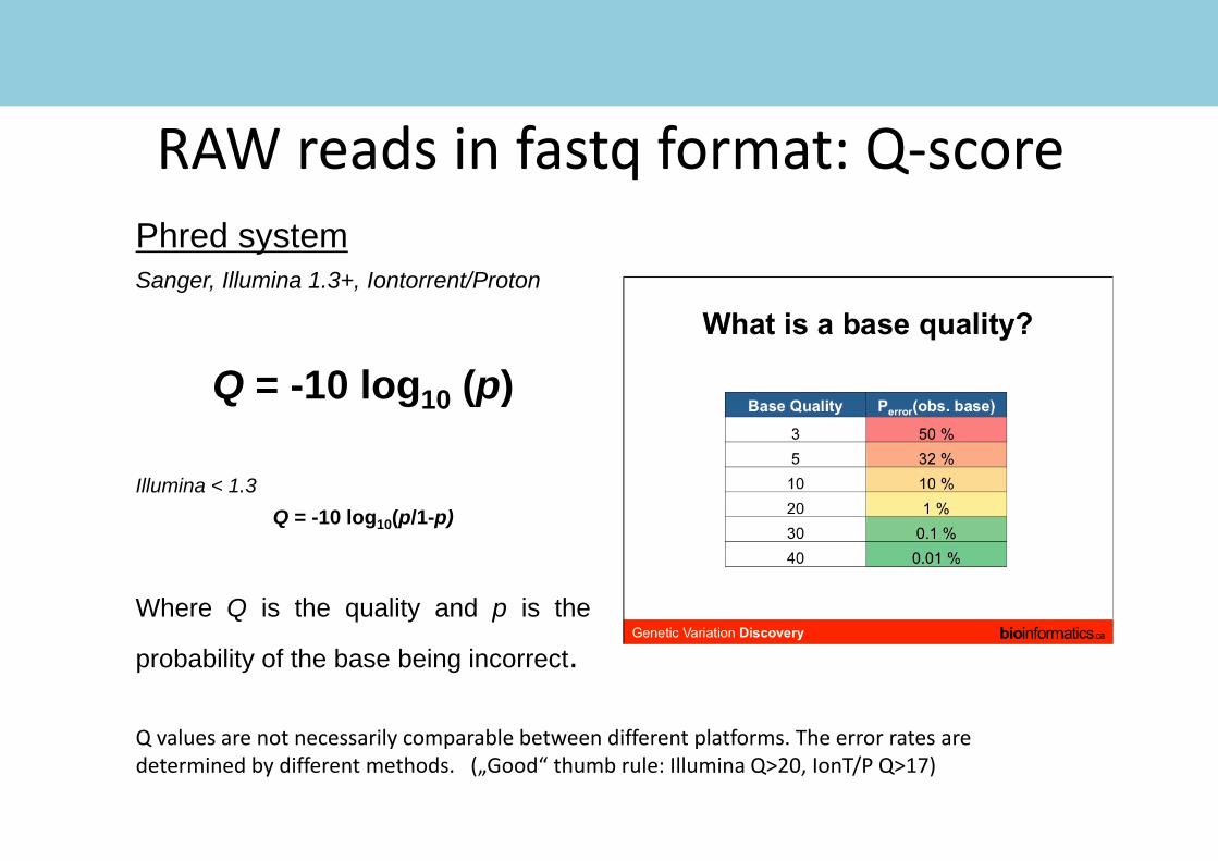
RAW reads in fastq format: Q‐scorePhred systemSanger, Illumina 1.3+, Iontorrent/Proton
Q = -10 log10 (p)
Illumina < 1.3Q = -10 log10(p/1-p)
Where Q is the quality and p is the
probability of the base being incorrect.
Q values are not necessarily comparable between different platforms. The error rates are determined by different methods. („Good“ thumb rule: Illumina Q>20, IonT/P Q>17)

RAW reads in fastq format: Q‐scoreQuality scores (numbers) are stored ASCII encoded in the fastq
IonT/P
Illumina (now)

Visualizing the meaning of Phred Scores
Accuracy
Error
20 and higher is generally a good score

Quality assessment using FastQC• Free Download
– Download: http://www.bioinformatics.babraham.ac.uk/projects/fastqc/
• Samples reads (200K default): fast, low resource use

Quality assessment using FastQC
BAD base quality(run or library issue)
leading bases!?(library artifact)

Quality assessment using FastQC
Adapter dimer contamination

Quality assessment using FastQC
Good Illumina data

How to get from BAD to Good?
?

How to get from BAD to Good?
Produce high quality data to begin with!
Filter out artifacts using “cleaning” tools!

Mapping adds informa)on : codified in SAM/BAM format
Enormous pile of short reads from HTS
Reference genome
Mapping and alignment algorithms
Reads mapped to reference
Mapping + cleanup
Variant Discovery
Variant EvaluaNo
n FASTQ -‐> BAM BAM -‐> VCF
from raw reads to aligned reads
from aligned reads to genomic variaNon
processing + analysis

Important file format #2: SAM/BAM (aligned reads)
SLX1:1:127:63:4 … 1 10052169 … 23M6N10M … GAAGATACTGGTTTTTTTCTTATGAGACGGAGT 768832'48::::::;;:/78$88818099897 NM:i:0 AS:i:30 XS:i:30 …
Read name
Locus
Alignment information
Read sequence
Quality scores
Meta data
Data processing
and analysis
BAM file allows us to represent the data of any sequencer. Analyses can then be conducted largely agnostic to the particular sequencer used.
A BAM file can contain data from a single or from several samples
-> technology-independent
Sequence Alignment Map / Binary Alignment Map (compressed)

BAM headers: an essen)al part of a BAM file
@HD VN:1.0 GO:none SO:coordinate @SQ SN:chrM LN:16571 @SQ SN:chr1 LN:247249719 @SQ SN:chr2 LN:242951149 [cut for clarity] @SQ SN:chr9 LN:140273252 @SQ SN:chr10 LN:135374737 @SQ SN:chr11 LN:134452384 [cut for clarity] @SQ SN:chr22 LN:49691432 @SQ SN:chrX LN:154913754 @SQ SN:chrY LN:57772954 @RG ID:20FUK.1 PL:illumina PU:20FUKAAXX100202.1 LB:Solexa-‐18483 SM:NA12878 CN:BI @RG ID:20FUK.2 PL:illumina PU:20FUKAAXX100202.2 LB:Solexa-‐18484 SM:NA12878 CN:BI @RG ID:20FUK.3 PL:illumina PU:20FUKAAXX100202.3 LB:Solexa-‐18483 SM:NA12878 CN:BI @RG ID:20FUK.4 PL:illumina PU:20FUKAAXX100202.4 LB:Solexa-‐18484 SM:NA12878 CN:BI @RG ID:20FUK.5 PL:illumina PU:20FUKAAXX100202.5 LB:Solexa-‐18483 SM:NA12878 CN:BI @RG ID:20FUK.6 PL:illumina PU:20FUKAAXX100202.6 LB:Solexa-‐18484 SM:NA12878 CN:BI @RG ID:20FUK.7 PL:illumina PU:20FUKAAXX100202.7 LB:Solexa-‐18483 SM:NA12878 CN:BI @RG ID:20FUK.8 PL:illumina PU:20FUKAAXX100202.8 LB:Solexa-‐18484 SM:NA12878 CN:BI @PG ID:BWA VN:0.5.7 CL:tk @PG ID:GATK PrintReads VN:1.0.2864 20FUKAAXX100202:1:1:12730:189900 163 chrM 1 60 101M = 282 381
GATCACAGGTCTATCACCCTATTAACCACTCACGGGAGCTCTCCATGCATTTGGTA…[more bases] ?BA@A>BBBBACBBAC@BBCBBCBC@BC@CAC@:BBCBBCACAACBABCBCCAB…[more quals] RG:Z:20FUK.1 NM:i:1 AM:i:37 MD:Z:72G28 MQ:i:60 PG:Z:BWA UQ:i:33
Required: Standard header
EssenNal: con)gs of aligned reference
sequence. Should be in karyotypic order.
EssenNal: read groups. Carries pla�orm (PL), library (LB), and sample (SM) informa)on. Each read is associated with a read
group
Useful: Data processing tools applied to the reads
Official specifica)on in hkp://samtools.sourceforge.net/SAM1.pdf

Variant calls are a summarized representa)on of the original sequence data
Mapping + cleanup
Variant Discovery
Variant EvaluaNo
n FASTQ -‐> BAM BAM -‐> VCF
from raw reads to aligned reads
from aligned reads to genomic variaNon
processing + analysis
Variant calling algorithms
site 1 descrip)on + sample genotypes
site 2 descrip)on + sample genotypes
site 3 descrip)on + sample genotypes

Important file format #3: VCF (genomic varia)on)
##fileformat=VCFv4.1 ##reference=1000GenomesPilot-NCBI36 ##INFO=<ID=DP,Number=1,Type=Integer,Description="Total Depth"> ##INFO=<ID=AF,Number=A,Type=Float,Description="Allele Frequency"> ##INFO=<ID=DB,Number=0,Type=Flag,Description="dbSNP membership"> ##FILTER=<ID=s50,Description="Less than 50% of samples have data"> ##FORMAT=<ID=GT,Number=1,Type=String,Description="Genotype"> ##FORMAT=<ID=GQ,Number=1,Type=Integer,Description="Genotype Quality"> ##FORMAT=<ID=DP,Number=1,Type=Integer,Description="Read Depth"> #CHROM POS ID REF ALT QUAL FILTER INFO
FORMAT NA00001 NA00002 NA00003
20 14370 rs6054257 G A 29 PASS DP=14;AF=0.5;DB GT:GQ:DP 0/0:48:1 1/0:48:8 1/1:43:5
20 1110696 rs6040355 A G,T 67 PASS DP=10;AF=0.333,0.667;DB
GT:GQ:DP 1/2:21:6 2/1:2:0 2/2:35:4
20 1230237 . T . 47 PASS DP=13 GT:GQ:DP 0/0:54:7 0/0:48:4 0/0:61:2
20 1234567 microsat1 GTCT G,GTACT 50 PASS DP=9
GT:GQ:DP 0/1:35:4 0/2:17:2 1/1:40:3
Header
Variant records
Official specifica)on in www.1000genomes.org/wiki/Analysis/Variant Call Format/vcf-‐variant-‐call-‐format-‐version-‐42

And that’s all you need to know to get started
Mapping + cleanup
Variant Discovery
Variant EvaluaNon
FASTQ -‐> BAM BAM -‐> VCF
from raw reads to aligned reads
from aligned reads to genomic variaNon
processing + analysis

• Toolkit focused on variant discovery (SNP & indel)
• Components:
- Engine and infrastructure
- Tools (walkers)
- Also a programming framework for developing genome analysis soGware
GATK = Genome Analysis Toolkit

GATK reads-‐to-‐variants workflow
Mapping + cleanup
Variant Discovery
Variant EvaluaTon
FASTQ -‐> BAM BAM -‐> VCF
+ other soUware (BWA, STAR, Picard, Samtools)
processing + analysis

• Java-‐based command line tool (see running requirements in FAQs)
• Consult online documenta)on for details about each tool! - Argument names and default values can change - Exact arguments depend on the given tool
java –jar GenomeAnalysisTK.jar –T ToolName \
–R reference.fasta \ –I inputBAM.bam \ –V inputVCF.vcf \ –o outputs.someformat \ –L 20:1000000-‐2000000
GATK command syntax

Soma)c Variant Discovery

Mapping and pre-‐processing
BWA + Picard/samtools + GATK Done separately for each sample in a tumor/normal pair

Overview of mapping & processing
Enormous pile of short reads from NGS
Reference genome
Key processing steps: • Map reads to the reference & clean up • Mark PCR duplicates • (RNAseq only) Process reads that span
splice juncMons

Ideally, we’d just align the sample genome to the reference genome
Region 1 Region 2 Region 3
truncated region duplicated region
= local variant (SNP/indel)
Reference
Sample
…But we don’t have the whole sample in one piece.

We have a pile of reads that need to be mapped individually
Enormous pile of short reads from
NGS
Region 1 Region 2 Region 3
Region 1 Region 2A Region 2B
Easy
Harder
Mapping is complicated by mismatches (true mutations or sequencing errors), indels, duplicated regions etc.

Mapping produces a SAM alignment summarizing position, quality, and structure for a given sequence
read1 99 ref 2 30 3M1D2M1I1M = 14 20 CATCTAG *
See also: • SAM format spec: hap://samtools.github.io/hts-‐specs/SAMv1.pdf • Explain SAM flags: hap://broadinsMtute.github.io/picard/explain-‐flags.html
POS (alignment start)
CIGAR (structure) SEQ (sequence) MAPQ (quality)
Mate informaDon

For DNAseq: map reads using BWA
The BWA soUware package by Heng Li & Richard Durbin hGp://bio-‐bwa.sourceforge.net/bwa.shtml
• “Burrows-‐Wheeler Aligner” • mem algorithm for 70bp or longer Illumina, 454, Ion Torrent and Sanger
reads, assembly conMgs and BAC sequences • Use –M flag to flag extra alignment hits as secondary (for downstream
compaMbility)

Generic recommendaMon for mapping starMng from FASTQ:
Reference genome
FASTQ
Mapped, cleaned, sorted SAM
• Use BWA MEM algorithm with –M flag and also –R to add read group info • OpMonally run Picard CleanSam and FixMateInformaMon and set
SO=coordinate • If you forgot to feed BWA the read group info, add it with Picard
AddOrReplaceReadGroups • Will not clip overhanging bases for short inserts!
BWA MEM Raw mapped SAM
CleanSam + FixMate

We now have properly mapped and sorted reads

Why mark duplicates?
Reference
Mapped reads
= sequencing error propagated in duplicates
• Duplicates are sets of reads pairs that have the same unclipped alignment start and unclipped alignment end
• They’re suspected to be non-‐independent measurements of a sequence • Sampled from the exact same template of DNA • Violates assumpMons of variant calling
• What’s more, errors in sample/library prep will get propagated to all the duplicates • Just pick the “best” copy – miMgates the effects of errors
Mark duplicates
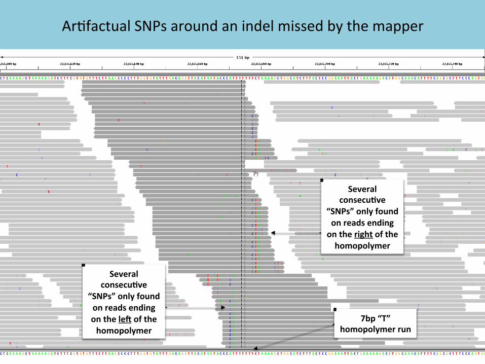
Ar7factual SNPs around an indel missed by the mapper
Several consecu2ve
“SNPs” only found on reads ending on the right of the homopolymer
Several consecu2ve
“SNPs” only found on reads ending on the le? of the homopolymer
7bp “T” homopolymer run

Why realign around indels?
• InDels in reads (especially near the ends) can trick the mappers into mis-‐aligning with mismatches
• These ar7factual mismatches can harm base quality recalibra7on and variant detec7on (unless a sophis7cated caller like MuTect2 is used)
þ Realignment around indels helps improve the accuracy of several of the downstream processing steps.

Local realignment uncovers the hidden indel in these reads and eliminates all the poten7al FP SNPs

Indel Realignment works in two phases
• Iden7fy what regions need to be realigned
• Perform the actual realignment

How do we find which regions need to be realigned?
• Known sites (e.g. dbSNP, 1000 Genomes)
• Indels seen in some of the read alignments (in CIGARs)
• Sites where evidence suggests a hidden indel (presence of mismatches and soRclips)
à Entropy calcula7on: Compute “ac7vity score” If above threshold per window include as realignment target

If we know there is a known indel at this site, we usually prefer to use that for the consensus, especially if there are several alternate possibili7es.
Known indels can be used to determine consensus
AAGAGTAGRef:
AAG---AGTAG
AAGAGTAG
Read pile consistent with CTA inser7on
Read pile consistent with the reference sequence Realigning
determines which is be[er
Three adjacent
SNPs
GGCTA
dbSNP

Is realignment s7ll necessary with latest soRware?
• Latest tools being implemented for variant discovery (HaplotypeCaller, MuTect 2, Platypus) all include some sort of assembly step (for which upstream realignment is not really helpful).
• BUT poten7al improvement for Base Quality Score Recalibra7on when run on realigned BAM files (ar7factual SNPs are replaced with real indels).
• Also s7ll useful for legacy tools, e.g. full realignment should be performed if using the GATK’s Unified Genotyper or MuTect for calling variants.
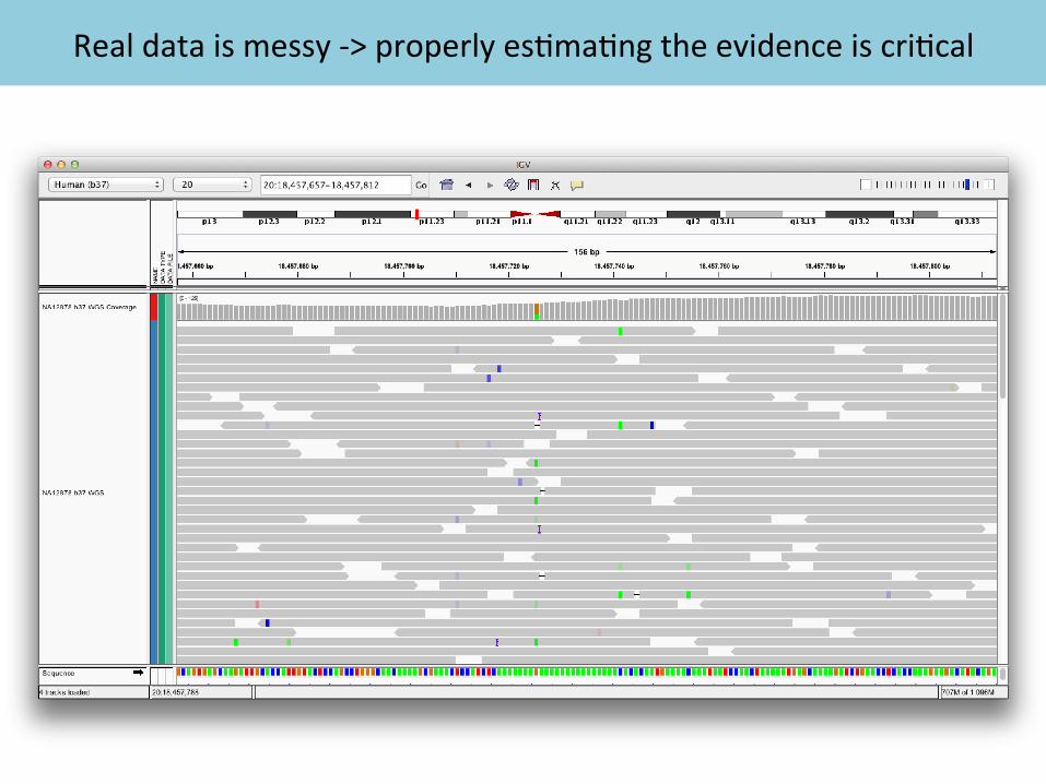
Real data is messy -‐> properly es2ma2ng the evidence is cri2cal

AA AG CA CG GA GG TA TG
−10
−5
05
10
RMSE = 4.188
Dinuc
Em
piric
al −
Report
ed Q
ualit
y
AA AG CA CG GA GG TA TG
−10
−5
05
10
RMSE = 0.281
Dinuc
Em
piric
al −
Report
ed Q
ualit
y
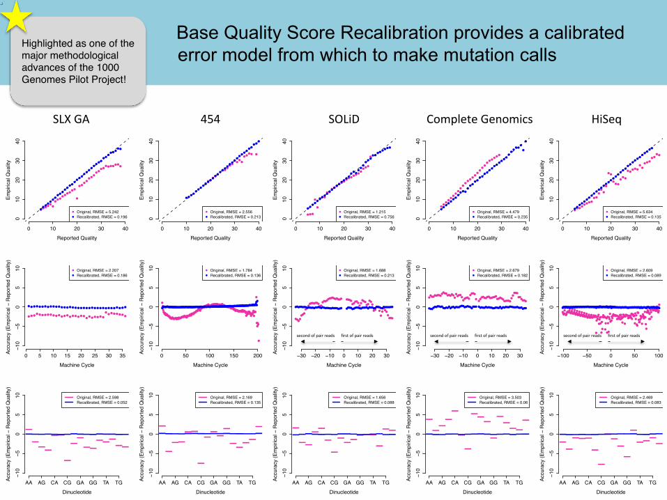
• Quality scores are cri2cal for all downstream analysis • Systema2c biases are a major contributor to bad calls
Example of bias: quali2es reported depending on nucleo2de context
original recalibrated
Quality scores emitted by sequencing machines are biased and inaccurate
BQSR method identifies bias and applies correction

Base Recalibra2on phases
• Model the error modes
• Apply recalibra2on and write to file
• Make before/aHer plots

• Systema2c errors correlate with basecall features
• Several relevant features: – Reported quality score – Posi2on within the read
(machine cycle) – Sequence context
(sequencing chemistry effects)
• Calculate error empirically and find paNerns in how error varies with basecall features
• Method is empowered by looking at en2re lane of data (works per read group)
How do we identify the error modes in the data?
AA AG CA CG GA GG TA TG
−10
−5
05
10
RMSE = 4.188
Dinuc
Em
piric
al −
Report
ed Q
ualit
y

Covariation patterns allow us to calculate adjustment factors
For each base in each read:
-‐ -‐ is it in AA context? -‐> adjust by X points -‐ -‐ ... -‐ -‐ is it at 3rd posi2on? -‐> adjust by Y points -‐ -‐ ...

• Any sequence mismatch = error except known variants*!
• Keep track of number of observa2ons and number of errors as a func2on of various error covariates (lane, original quality score, machine cycle, and sequencing context)
# of reference mismatches+1# of observed bases+ 2
PHRED-‐scaled quality score
How do we derive the adjustment factors used for recalibration?
* If you don’t have known varia=on, bootstrap (see later on)
SLX GA 454 SOLiD HiSeq Complete Genomics
●●●●
●●
●●●
●●●●
●●
●
●
●●
●●
●●
●●
●●●●●● ●
●●
0 10 20 30 40
010
20
30
40
Reported Quality
Em
pir
ical Q
ualit
y
●●●●●●●●●●●
●●
●●
●●
●●
●●
●●
●●
●●
●●
●●
●●●
●
●
Original, RMSE = 5.242
Recalibrated, RMSE = 0.196
●●
●●
●●●
●●
●●
●●
●●
●
●●●●
0 10 20 30 40
010
20
30
40
Reported Quality
Em
pir
ical Q
ualit
y
●●●●●●
●●
●●
●●
●●
●●
●●
●●
●●
●●
●●
●●
●●
●
●
●
Original, RMSE = 2.556
Recalibrated, RMSE = 0.213●●●
●
●
●●●
●●●
●●
●●
●●
●●
●●
●●
●●
●
●
0 10 20 30 40
010
20
30
40
Reported Quality
Em
pir
ical Q
ualit
y
●●●●●●●●●●●
●●
●●
●●
●●
●●
●●
●●
●●
●●●●
●●●●
●
●
Original, RMSE = 1.215
Recalibrated, RMSE = 0.756
●●●●●●●●●●●
●●
●●
●●
●●
●●
●●
●●
0 10 20 30 40
010
20
30
40
Reported Quality
Em
pir
ical Q
ualit
y
●●●●●●●●●●●
●●
●●
●●
●●
●●
●●
●●
●●
●●
●●
●
●●●
●
●
●
Original, RMSE = 4.479
Recalibrated, RMSE = 0.235
●●●
●●●
●●
●●
● ●●
●
●
●
●
●●
●●
●
●
●●
●●
●●●●
●●
●●
●
0 10 20 30 40
010
20
30
40
Reported Quality
Em
pir
ical Q
ualit
y
●●●●●●●●●●●
●●
●●
●●
●●
●●
●●
●●
●●
●●
●●
●●
●
●
Original, RMSE = 5.634
Recalibrated, RMSE = 0.135
●●●●●●●●●●●●●●● ●● ●● ●● ●
● ●● ●●
●
●
●● ●●●●●
0 5 10 15 20 25 30 35
−10
−5
05
10
Machine Cycle
Accura
cy (
Em
pir
ical −
Report
ed Q
ualit
y)
●●●●●●●●●●●●●●● ●● ●● ●● ●● ●● ●● ●● ●● ●●●● ●
●
●
Original, RMSE = 2.207
Recalibrated, RMSE = 0.186
●
●
●●●●●●●●●●●●●●●●●●●●●●●●●●●●●●●●●●●
●●●●●●●●●●●●●●●●●●
●●●●●●●●●●●●●●●●
●●●●
●●●●
●●●●●●●●
●●●●●●●●●●●●●●●
● ●●●●●●●● ●●●●●●●● ●
●●●●●●●
●●●●●●●●●●●●●●●●
●●●●●●●●●●●●●●●●
●●●●
●●●●●●●●●●●●
●●●●●●●●●●●
●●●●●
●●
●
●
●
●●
●
●
●●
0 50 100 150 200
−10
−5
05
10
Machine Cycle
Accura
cy (
Em
pir
ical −
Report
ed Q
ualit
y)
●●●●●●●●●●●●●●●●●●●●●●●●●●●●●●●●●●●●●●●●●●●●●●●●●●●●●●●●●●●●●●● ●●●●●●●● ●●●●●●●● ●●●●●●●● ●●●●●●●● ●●●●●●●● ●●●●●●●● ●●●●●●●● ●●●●●●●● ●●●●●●●●●●●●●●●● ●●●●●●●●●●●●●●●● ●●●●●●●●●●●●●●●● ●●●●●●●●●●●●●●●●
●●●
●●●●●
●
●
Original, RMSE = 1.784
Recalibrated, RMSE = 0.136
●●
●
●
●
●
●
●
●
●
●●
●
●●●
●●
● ●●●
● ●●●
●
●●
●
●●
●●
●● ●●
●
●
●
●
●
●
●
●
●
●
●
●
●
●
●
●
●
●
●
●
●
●
●
●●●●●
−30 −20 −10 0 10 20 30
−10
−5
05
10
Machine Cycle
Accura
cy (
Em
pir
ical −
Report
ed Q
ualit
y)
●●●
●● ●● ●● ●●●● ●● ●● ●● ●● ●● ●● ●● ●● ●● ●● ●● ●● ●● ●● ●● ●
● ●● ●● ●●● ●●●●
●● ●● ● ●●●●●
●
●
Original, RMSE = 1.688
Recalibrated, RMSE = 0.213
●●
●
●●
●●
●●
●●
●
●● ●
●●
●
●●
●
●
●● ●● ●●
●
●
●●● ●
●
●
●●
●
●
●
●
●
●● ●●
●● ●●
●
●
●●
●
● ●●
●
●●
●●●●
●●
−30 −20 −10 0 10 20 30
−10
−5
05
10
Machine Cycle
Accura
cy (
Em
pir
ical −
Report
ed Q
ualit
y)
● ●●
● ●● ●● ●●
●● ●● ●● ●● ●● ●● ●● ●● ●● ●● ●● ●
● ● ●● ●● ●● ●● ●● ●● ●● ●● ●● ●● ●● ●● ●●● ● ●●●●●
●
●
Original, RMSE = 2.679
Recalibrated, RMSE = 0.182
●
●●●●●●●●●●●
●●●●●●●●
●●●●
●
●●
●
●●●●●●●●●●●●
●
●●●●●
●●
●
●●
●●
●
●●●
●●
●●
●●
●●●
●
●
●
●●
●●●●
●
●
●
●
●
●●●
●
●
●
●
●●●●●●●● ●
●
●●
●●
●
●●●
●●
●
●●●●
●●
●
●
●
●●●●
●
●
●●
●
●
●
●
●●
●
●
●●●●●●●●●●●
●
●●●●●
●●●●●●●●●●●●●
●●
●
●●●●
●
●●●●
●●●●●
●●
●●●●●●●
●●●●
●●
●●●●●●●
−100 −50 0 50 100
−10
−5
05
10
Machine Cycle
Accura
cy (
Em
pir
ical −
Report
ed Q
ualit
y)
●●●●●●●●●●●●●●●●●●●●●●●●●●●●●●●●●●●●●●●●●●●●●●●●●●●●●●●●●●●●●●● ●●●●●●●● ●●●●●●●● ●●●●●●●● ●●●●●●●● ●●●●●●●●●●●●●●●●●●●●●●●●●●●●●●●●●●●●●●●●●●●●●●●●●●●●●●●●●●●●●●●●●●●●●●●●●●●●●● ●●●●●●●● ●●●●●●●● ●●●●●●●●●●●●●
●
●
Original, RMSE = 2.609
Recalibrated, RMSE = 0.089
−10
−5
05
10
Dinucleotide
Accura
cy (
Em
pir
ical −
Report
ed Q
ualit
y)
−
−−−
−−
−
−−−−−−−−−
−−−−−−−−−−−−−−−−
AA AG CA CG GA GG TA TG
Original, RMSE = 2.598
Recalibrated, RMSE = 0.052
−10
−5
05
10
Dinucleotide
Accura
cy (
Em
pir
ical −
Report
ed Q
ualit
y)
−
−−−−−
−
−−−−
−−−−
−−−−−−−−−−−−−−−−−
AA AG CA CG GA GG TA TG
Original, RMSE = 2.169
Recalibrated, RMSE = 0.135
−10
−5
05
10
Dinucleotide
Accura
cy (
Em
pir
ical −
Report
ed Q
ualit
y)
−
−−
−−−
−
−−−−−−
−
−−−−−−−−−−−−−−−−−−
AA AG CA CG GA GG TA TG
Original, RMSE = 1.656
Recalibrated, RMSE = 0.088
−10
−5
05
10
Dinucleotide
Accura
cy (
Em
pir
ical −
Report
ed Q
ualit
y)
−−−−−
−
−
−−−
−
−−−−−
−−−−−−−−−−−−−−−−
AA AG CA CG GA GG TA TG
Original, RMSE = 3.503
Recalibrated, RMSE = 0.06
−10
−5
05
10
Dinucleotide
Accura
cy (
Em
pir
ical −
Report
ed Q
ualit
y)
−−−−−
−
−
−−−−
−
−−−−−−−−−−−−−−−−−−−−
AA AG CA CG GA GG TA TG
Original, RMSE = 2.469
Recalibrated, RMSE = 0.083
first of pair reads second of pair reads first of pair reads second of pair reads first of pair reads second of pair reads
Base Qu Base Quality Score Recalibration provides a calibrated error model from which to make mutation calls
Highlighted as one of the major methodological advances of the 1000 Genomes Pilot Project!

Base Recalibra2on workflow: data processing path
Recalibra2on table
Recalibrated BAM file
BaseRecalibrator
PrintReads
Original BAM file + Known sites

BaseRecalibrator
• Builds recalibra2on model
java –jar GenomeAnalysisTK.jar –T BaseRecalibrator \
–R human.fasta \ –I realigned.bam \ –knownSites dbsnp137.vcf \ –knownSites gold.standard.indels.vcf \
[ –L exome_targets.intervals \ ] –o recal.table

Why specify –L intervals when running BaseRecalibrator on WEx?
• BQSR depends on key assump2on: every mismatch is an error, except sites in known variants
• Off-‐target sequence likely to have higher error rates with different error modes
• If off-‐target sequence is included in recalibra2on, may skew the model and mess up results
Ø Use –L argument with BaseRecalibrator to restrict recalibra=on to capture targets.

Print Reads
• General-‐use tool co-‐opted with –BQSR flag and fed a recalibra2on report
• Creates a new bam file using the input table generated previously which has exquisitely accurate base subs2tu2on, inser2on, and dele2on quality scores
• Original quali2es can be retained with OQ tag (not default)
java –jar GenomeAnalysisTK.jar –T PrintReads \
–R human.fasta \ –I realigned.bam \ –BQSR recal.table \ –o recal.bam

… and subs2tute the ploing workflow
Recalibra2on table (1)
BaseRecalibrator (1)
Original BAM file + Known sites
Recalibra2on table (2)
BaseRecalibrator (2) Plots
AnalyzeCovariates

Base Recalibrator
• Second pass evaluates what the data looks like aHer recalibra2on
java –jar GenomeAnalysisTK.jar –T BaseRecalibrator \
–R human.fasta \ –I realigned.bam \ –knownSites dbsnp137.vcf \ –knownSites gold.standard.indels.vcf \ –BQSR recal.table \ –o a[er_recal.table

AnalyzeCovariates
• Makes plots based on before/aHer recalibra2on tables
• There is an op2on to keep the intermediate .csv file used for ploing, if you want to play with the plot data.
java –jar GenomeAnalysisTK.jar –T AnalyzeCovariates \
–R human.fasta \ –before recal.table \ –a[er a[er_recal.table \ –plots recal_plots.pdf

42
Post-‐recalibra2on quality scores should fit the empirically-‐derived quality scores very well; no obvious systema2c biases should remain
●●●●
●●
●●●
●●●●
●●
●
●
●●
●●
●●
●●
●●●●●● ●
●●
0 10 20 30 40
01
02
03
04
0
Reported Quality
Em
pir
ica
l Q
ua
lity
●●●●●●●●●●●
●●
●●
●●
●●
●●
●●
●●
●●
●●
●●
●●●
●
●
Original, RMSE = 5.242
Recalibrated, RMSE = 0.196
●●
●●
●●●
●●
●●
●●
●●
●
●●●●
0 10 20 30 40
01
02
03
04
0
Reported Quality
Em
pir
ica
l Q
ua
lity
●●●●●●
●●
●●
●●
●●
●●
●●
●●
●●
●●
●●
●●
●●
●
●
●
Original, RMSE = 2.556
Recalibrated, RMSE = 0.213●●●
●
●
●●●
●●●
●●
●●
●●
●●
●●
●●
●●
●
●
0 10 20 30 40
01
02
03
04
0
Reported Quality
Em
pir
ica
l Q
ua
lity
●●●●●●●●●●●
●●
●●
●●
●●
●●
●●
●●
●●
●●●●
●●●●
●
●
Original, RMSE = 1.215
Recalibrated, RMSE = 0.756
●●●●●●●●●●●
●●
●●
●●
●●
●●
●●
●●
0 10 20 30 40
01
02
03
04
0
Reported Quality
Em
pir
ica
l Q
ua
lity
●●●●●●●●●●●
●●
●●
●●
●●
●●
●●
●●
●●
●●
●●
●
●●●
●
●
●
Original, RMSE = 4.479
Recalibrated, RMSE = 0.235
●●●
●●●
●●
●●
● ●●
●
●
●
●
●●
●●
●
●
●●
●●
●●●●
●●
●●
●
0 10 20 30 40
01
02
03
04
0
Reported Quality
Em
pir
ica
l Q
ua
lity
●●●●●●●●●●●
●●
●●
●●
●●
●●
●●
●●
●●
●●
●●
●●
●
●
Original, RMSE = 5.634
Recalibrated, RMSE = 0.135
●●●●●●●●●●●●●●● ●● ●● ●● ●
● ●● ●●
●
●
●● ●●●●●
0 5 10 15 20 25 30 35
−1
0−
50
51
0
Machine Cycle
Accu
racy (
Em
pir
ica
l −
Re
po
rte
d Q
ua
lity)
●●●●●●●●●●●●●●● ●● ●● ●● ●● ●● ●● ●● ●● ●●●● ●
●
●
Original, RMSE = 2.207
Recalibrated, RMSE = 0.186
●
●
●●●●●●●●●●●●●●●●●●●●●●●●●●●●●●●●●●●
●●●●●●●●●●●●●●●●●●
●●●●●●●●●●●●●●●●
●●●●
●●●●
●●●●●●●●
●●●●●●●●●●●●●●●
● ●●●●●●●● ●●●●●●●● ●
●●●●●●●
●●●●●●●●●●●●●●●●
●●●●●●●●●●●●●●●●
●●●●
●●●●●●●●●●●●
●●●●●●●●●●●
●●●●●
●●
●
●
●
●●
●
●
●●
0 50 100 150 200
−1
0−
50
51
0
Machine Cycle
Accu
racy (
Em
pir
ica
l −
Re
po
rte
d Q
ua
lity)
●●●●●●●●●●●●●●●●●●●●●●●●●●●●●●●●●●●●●●●●●●●●●●●●●●●●●●●●●●●●●●● ●●●●●●●● ●●●●●●●● ●●●●●●●● ●●●●●●●● ●●●●●●●● ●●●●●●●● ●●●●●●●● ●●●●●●●● ●●●●●●●●●●●●●●●● ●●●●●●●●●●●●●●●● ●●●●●●●●●●●●●●●● ●●●●●●●●●●●●●●●●
●●●
●●●●●
●
●
Original, RMSE = 1.784
Recalibrated, RMSE = 0.136
●●
●
●
●
●
●
●
●
●
●●
●
●●●
●●
● ●●●
● ●●●
●
●●
●
●●
●●
●● ●●
●
●
●
●
●
●
●
●
●
●
●
●
●
●
●
●
●
●
●
●
●
●
●
●●●●●
−30 −20 −10 0 10 20 30
−1
0−
50
51
0
Machine Cycle
Accu
racy (
Em
pir
ica
l −
Re
po
rte
d Q
ua
lity)
●●●
●● ●● ●● ●●●● ●● ●● ●● ●● ●● ●● ●● ●● ●● ●● ●● ●● ●● ●● ●● ●
● ●● ●● ●●● ●●●●
●● ●● ● ●●●●●
●
●
Original, RMSE = 1.688
Recalibrated, RMSE = 0.213
●●
●
●●
●●
●●
●●
●
●● ●
●●
●
●●
●
●
●● ●● ●●
●
●
●●● ●
●
●
●●
●
●
●
●
●
●● ●●
●● ●●
●
●
●●
●
● ●●
●
●●
●●●●
●●
−30 −20 −10 0 10 20 30
−1
0−
50
51
0
Machine Cycle
Accu
racy (
Em
pir
ica
l −
Re
po
rte
d Q
ua
lity)
● ●●
● ●● ●● ●●
●● ●● ●● ●● ●● ●● ●● ●● ●● ●● ●● ●
● ● ●● ●● ●● ●● ●● ●● ●● ●● ●● ●● ●● ●● ●●● ● ●●●●●
●
●
Original, RMSE = 2.679
Recalibrated, RMSE = 0.182
●
●●●●●●●●●●●
●●●●●●●●
●●●●
●
●●
●
●●●●●●●●●●●●
●
●●●●●
●●
●
●●
●●
●
●●●
●●
●●
●●
●●●
●
●
●
●●
●●●●
●
●
●
●
●
●●●
●
●
●
●
●●●●●●●● ●
●
●●
●●
●
●●●
●●
●
●●●●
●●
●
●
●
●●●●
●
●
●●
●
●
●
●
●●
●
●
●●●●●●●●●●●
●
●●●●●
●●●●●●●●●●●●●
●●
●
●●●●
●
●●●●
●●●●●
●●
●●●●●●●
●●●●
●●
●●●●●●●
−100 −50 0 50 100
−1
0−
50
51
0
Machine Cycle
Accu
racy (
Em
pir
ica
l −
Re
po
rte
d Q
ua
lity)
●●●●●●●●●●●●●●●●●●●●●●●●●●●●●●●●●●●●●●●●●●●●●●●●●●●●●●●●●●●●●●● ●●●●●●●● ●●●●●●●● ●●●●●●●● ●●●●●●●● ●●●●●●●●●●●●●●●●●●●●●●●●●●●●●●●●●●●●●●●●●●●●●●●●●●●●●●●●●●●●●●●●●●●●●●●●●●●●●● ●●●●●●●● ●●●●●●●● ●●●●●●●●●●●●●
●
●
Original, RMSE = 2.609
Recalibrated, RMSE = 0.089
−1
0−
50
51
0
Dinucleotide
Accu
racy (
Em
pir
ica
l −
Re
po
rte
d Q
ua
lity)
−
−−−
−−
−
−−−−−−−−−
−−−−−−−−−−−−−−−−
AA AG CA CG GA GG TA TG
Original, RMSE = 2.598
Recalibrated, RMSE = 0.052
−1
0−
50
51
0
Dinucleotide
Accu
racy (
Em
pir
ica
l −
Re
po
rte
d Q
ua
lity)
−
−−−−−
−
−−−−
−−−−
−−−−−−−−−−−−−−−−−
AA AG CA CG GA GG TA TG
Original, RMSE = 2.169
Recalibrated, RMSE = 0.135
−1
0−
50
51
0
Dinucleotide
Accu
racy (
Em
pir
ica
l −
Re
po
rte
d Q
ua
lity)
−
−−
−−−
−
−−−−−−
−
−−−−−−−−−−−−−−−−−−
AA AG CA CG GA GG TA TG
Original, RMSE = 1.656
Recalibrated, RMSE = 0.088
−1
0−
50
51
0
Dinucleotide
Accu
racy (
Em
pir
ica
l −
Re
po
rte
d Q
ua
lity)
−−−−−
−
−
−−−
−
−−−−−
−−−−−−−−−−−−−−−−
AA AG CA CG GA GG TA TG
Original, RMSE = 3.503
Recalibrated, RMSE = 0.06
−1
0−
50
51
0
Dinucleotide
Accu
racy (
Em
pir
ica
l −
Re
po
rte
d Q
ua
lity)
−−−−−
−
−
−−−−
−
−−−−−−−−−−−−−−−−−−−−
AA AG CA CG GA GG TA TG
Original, RMSE = 2.469
Recalibrated, RMSE = 0.083
●●●●
●●
●●●
●●●●
●●
●
●
●●
●●
●●
●●
●●●●●● ●
●●
0 10 20 30 40
01
02
03
04
0
Reported Quality
Em
pir
ica
l Q
ua
lity
●●●●●●●●●●●
●●
●●
●●
●●
●●
●●
●●
●●
●●
●●
●●●
●
●
Original, RMSE = 5.242
Recalibrated, RMSE = 0.196
●●
●●
●●●
●●
●●
●●
●●
●
●●●●
0 10 20 30 40
01
02
03
04
0
Reported Quality
Em
pir
ica
l Q
ua
lity
●●●●●●
●●
●●
●●
●●
●●
●●
●●
●●
●●
●●
●●
●●
●
●
●
Original, RMSE = 2.556
Recalibrated, RMSE = 0.213●●●
●
●
●●●
●●●
●●
●●
●●
●●
●●
●●
●●
●
●
0 10 20 30 40
01
02
03
04
0
Reported Quality
Em
pir
ica
l Q
ua
lity
●●●●●●●●●●●
●●
●●
●●
●●
●●
●●
●●
●●
●●●●
●●●●
●
●
Original, RMSE = 1.215
Recalibrated, RMSE = 0.756
●●●●●●●●●●●
●●
●●
●●
●●
●●
●●
●●
0 10 20 30 40
01
02
03
04
0
Reported Quality
Em
pir
ica
l Q
ua
lity
●●●●●●●●●●●
●●
●●
●●
●●
●●
●●
●●
●●
●●
●●
●
●●●
●
●
●
Original, RMSE = 4.479
Recalibrated, RMSE = 0.235
●●●
●●●
●●
●●
● ●●
●
●
●
●
●●
●●
●
●
●●
●●
●●●●
●●
●●
●
0 10 20 30 40
01
02
03
04
0
Reported QualityE
mp
iric
al Q
ua
lity
●●●●●●●●●●●
●●
●●
●●
●●
●●
●●
●●
●●
●●
●●
●●
●
●
Original, RMSE = 5.634
Recalibrated, RMSE = 0.135
●●●●●●●●●●●●●●● ●● ●● ●● ●
● ●● ●●
●
●
●● ●●●●●
0 5 10 15 20 25 30 35
−1
0−
50
51
0
Machine Cycle
Accu
racy (
Em
pir
ica
l −
Re
po
rte
d Q
ua
lity)
●●●●●●●●●●●●●●● ●● ●● ●● ●● ●● ●● ●● ●● ●●●● ●
●
●
Original, RMSE = 2.207
Recalibrated, RMSE = 0.186
●
●
●●●●●●●●●●●●●●●●●●●●●●●●●●●●●●●●●●●
●●●●●●●●●●●●●●●●●●
●●●●●●●●●●●●●●●●
●●●●
●●●●
●●●●●●●●
●●●●●●●●●●●●●●●
● ●●●●●●●● ●●●●●●●● ●
●●●●●●●
●●●●●●●●●●●●●●●●
●●●●●●●●●●●●●●●●
●●●●
●●●●●●●●●●●●
●●●●●●●●●●●
●●●●●
●●
●
●
●
●●
●
●
●●
0 50 100 150 200
−1
0−
50
51
0
Machine Cycle
Accu
racy (
Em
pir
ica
l −
Re
po
rte
d Q
ua
lity)
●●●●●●●●●●●●●●●●●●●●●●●●●●●●●●●●●●●●●●●●●●●●●●●●●●●●●●●●●●●●●●● ●●●●●●●● ●●●●●●●● ●●●●●●●● ●●●●●●●● ●●●●●●●● ●●●●●●●● ●●●●●●●● ●●●●●●●● ●●●●●●●●●●●●●●●● ●●●●●●●●●●●●●●●● ●●●●●●●●●●●●●●●● ●●●●●●●●●●●●●●●●
●●●
●●●●●
●
●
Original, RMSE = 1.784
Recalibrated, RMSE = 0.136
●●
●
●
●
●
●
●
●
●
●●
●
●●●
●●
● ●●●
● ●●●
●
●●
●
●●
●●
●● ●●
●
●
●
●
●
●
●
●
●
●
●
●
●
●
●
●
●
●
●
●
●
●
●
●●●●●
−30 −20 −10 0 10 20 30
−1
0−
50
51
0
Machine Cycle
Accu
racy (
Em
pir
ica
l −
Re
po
rte
d Q
ua
lity)
●●●
●● ●● ●● ●●●● ●● ●● ●● ●● ●● ●● ●● ●● ●● ●● ●● ●● ●● ●● ●● ●
● ●● ●● ●●● ●●●●
●● ●● ● ●●●●●
●
●
Original, RMSE = 1.688
Recalibrated, RMSE = 0.213
●●
●
●●
●●
●●
●●
●
●● ●
●●
●
●●
●
●
●● ●● ●●
●
●
●●● ●
●
●
●●
●
●
●
●
●
●● ●●
●● ●●
●
●
●●
●
● ●●
●
●●
●●●●
●●
−30 −20 −10 0 10 20 30
−1
0−
50
51
0
Machine Cycle
Accu
racy (
Em
pir
ica
l −
Re
po
rte
d Q
ua
lity)
● ●●
● ●● ●● ●●
●● ●● ●● ●● ●● ●● ●● ●● ●● ●● ●● ●
● ● ●● ●● ●● ●● ●● ●● ●● ●● ●● ●● ●● ●● ●●● ● ●●●●●
●
●
Original, RMSE = 2.679
Recalibrated, RMSE = 0.182
●
●●●●●●●●●●●
●●●●●●●●
●●●●
●
●●
●
●●●●●●●●●●●●
●
●●●●●
●●
●
●●
●●
●
●●●
●●
●●
●●
●●●
●
●
●
●●
●●●●
●
●
●
●
●
●●●
●
●
●
●
●●●●●●●● ●
●
●●
●●
●
●●●
●●
●
●●●●
●●
●
●
●
●●●●
●
●
●●
●
●
●
●
●●
●
●
●●●●●●●●●●●
●
●●●●●
●●●●●●●●●●●●●
●●
●
●●●●
●
●●●●
●●●●●
●●
●●●●●●●
●●●●
●●
●●●●●●●
−100 −50 0 50 100
−1
0−
50
51
0
Machine Cycle
Accu
racy (
Em
pir
ica
l −
Re
po
rte
d Q
ua
lity)
●●●●●●●●●●●●●●●●●●●●●●●●●●●●●●●●●●●●●●●●●●●●●●●●●●●●●●●●●●●●●●● ●●●●●●●● ●●●●●●●● ●●●●●●●● ●●●●●●●● ●●●●●●●●●●●●●●●●●●●●●●●●●●●●●●●●●●●●●●●●●●●●●●●●●●●●●●●●●●●●●●●●●●●●●●●●●●●●●● ●●●●●●●● ●●●●●●●● ●●●●●●●●●●●●●
●
●
Original, RMSE = 2.609
Recalibrated, RMSE = 0.089
−1
0−
50
51
0
Dinucleotide
Accu
racy (
Em
pir
ica
l −
Re
po
rte
d Q
ua
lity)
−
−−−
−−
−
−−−−−−−−−
−−−−−−−−−−−−−−−−
AA AG CA CG GA GG TA TG
Original, RMSE = 2.598
Recalibrated, RMSE = 0.052
−1
0−
50
51
0
Dinucleotide
Accu
racy (
Em
pir
ica
l −
Re
po
rte
d Q
ua
lity)
−
−−−−−
−
−−−−
−−−−
−−−−−−−−−−−−−−−−−
AA AG CA CG GA GG TA TG
Original, RMSE = 2.169
Recalibrated, RMSE = 0.135
−1
0−
50
51
0
Dinucleotide
Accu
racy (
Em
pir
ica
l −
Re
po
rte
d Q
ua
lity)
−
−−
−−−
−
−−−−−−
−
−−−−−−−−−−−−−−−−−−
AA AG CA CG GA GG TA TG
Original, RMSE = 1.656
Recalibrated, RMSE = 0.088
−1
0−
50
51
0
Dinucleotide
Accu
racy (
Em
pir
ica
l −
Re
po
rte
d Q
ua
lity)
−−−−−
−
−
−−−
−
−−−−−
−−−−−−−−−−−−−−−−
AA AG CA CG GA GG TA TG
Original, RMSE = 3.503
Recalibrated, RMSE = 0.06
−1
0−
50
51
0
Dinucleotide
Accu
racy (
Em
pir
ica
l −
Re
po
rte
d Q
ua
lity)
−−−−−
−
−
−−−−
−
−−−−−−−−−−−−−−−−−−−−
AA AG CA CG GA GG TA TG
Original, RMSE = 2.469
Recalibrated, RMSE = 0.083
●●●●
●●
●●●
●●●●
●●
●
●
●●
●●
●●
●●
●●●●●● ●
●●
0 10 20 30 40
01
02
03
04
0
Reported Quality
Em
pir
ica
l Q
ua
lity
●●●●●●●●●●●
●●
●●
●●
●●
●●
●●
●●
●●
●●
●●
●●●
●
●
Original, RMSE = 5.242
Recalibrated, RMSE = 0.196
●●
●●
●●●
●●
●●
●●
●●
●
●●●●
0 10 20 30 40
01
02
03
04
0
Reported Quality
Em
pir
ica
l Q
ua
lity
●●●●●●
●●
●●
●●
●●
●●
●●
●●
●●
●●
●●
●●
●●
●
●
●
Original, RMSE = 2.556
Recalibrated, RMSE = 0.213●●●
●
●
●●●
●●●
●●
●●
●●
●●
●●
●●
●●
●
●
0 10 20 30 40
01
02
03
04
0
Reported Quality
Em
pir
ica
l Q
ua
lity
●●●●●●●●●●●
●●
●●
●●
●●
●●
●●
●●
●●
●●●●
●●●●
●
●
Original, RMSE = 1.215
Recalibrated, RMSE = 0.756
●●●●●●●●●●●
●●
●●
●●
●●
●●
●●
●●
0 10 20 30 40
01
02
03
04
0
Reported Quality
Em
pir
ica
l Q
ua
lity
●●●●●●●●●●●
●●
●●
●●
●●
●●
●●
●●
●●
●●
●●
●
●●●
●
●
●
Original, RMSE = 4.479
Recalibrated, RMSE = 0.235
●●●
●●●
●●
●●
● ●●
●
●
●
●
●●
●●
●
●
●●
●●
●●●●
●●
●●
●
0 10 20 30 40
01
02
03
04
0
Reported Quality
Em
pir
ica
l Q
ua
lity
●●●●●●●●●●●
●●
●●
●●
●●
●●
●●
●●
●●
●●
●●
●●
●
●
Original, RMSE = 5.634
Recalibrated, RMSE = 0.135
●●●●●●●●●●●●●●● ●● ●● ●● ●
● ●● ●●
●
●
●● ●●●●●
0 5 10 15 20 25 30 35
−1
0−
50
51
0
Machine Cycle
Accu
racy (
Em
pir
ica
l −
Re
po
rte
d Q
ua
lity)
●●●●●●●●●●●●●●● ●● ●● ●● ●● ●● ●● ●● ●● ●●●● ●
●
●
Original, RMSE = 2.207
Recalibrated, RMSE = 0.186
●
●
●●●●●●●●●●●●●●●●●●●●●●●●●●●●●●●●●●●
●●●●●●●●●●●●●●●●●●
●●●●●●●●●●●●●●●●
●●●●
●●●●
●●●●●●●●
●●●●●●●●●●●●●●●
● ●●●●●●●● ●●●●●●●● ●
●●●●●●●
●●●●●●●●●●●●●●●●
●●●●●●●●●●●●●●●●
●●●●
●●●●●●●●●●●●
●●●●●●●●●●●
●●●●●
●●
●
●
●
●●
●
●
●●
0 50 100 150 200
−1
0−
50
51
0
Machine Cycle
Accu
racy (
Em
pir
ica
l −
Re
po
rte
d Q
ua
lity)
●●●●●●●●●●●●●●●●●●●●●●●●●●●●●●●●●●●●●●●●●●●●●●●●●●●●●●●●●●●●●●● ●●●●●●●● ●●●●●●●● ●●●●●●●● ●●●●●●●● ●●●●●●●● ●●●●●●●● ●●●●●●●● ●●●●●●●● ●●●●●●●●●●●●●●●● ●●●●●●●●●●●●●●●● ●●●●●●●●●●●●●●●● ●●●●●●●●●●●●●●●●
●●●
●●●●●
●
●
Original, RMSE = 1.784
Recalibrated, RMSE = 0.136
●●
●
●
●
●
●
●
●
●
●●
●
●●●
●●
● ●●●
● ●●●
●
●●
●
●●
●●
●● ●●
●
●
●
●
●
●
●
●
●
●
●
●
●
●
●
●
●
●
●
●
●
●
●
●●●●●
−30 −20 −10 0 10 20 30
−1
0−
50
51
0
Machine Cycle
Accu
racy (
Em
pir
ica
l −
Re
po
rte
d Q
ua
lity)
●●●
●● ●● ●● ●●●● ●● ●● ●● ●● ●● ●● ●● ●● ●● ●● ●● ●● ●● ●● ●● ●
● ●● ●● ●●● ●●●●
●● ●● ● ●●●●●
●
●
Original, RMSE = 1.688
Recalibrated, RMSE = 0.213
●●
●
●●
●●
●●
●●
●
●● ●
●●
●
●●
●
●
●● ●● ●●
●
●
●●● ●
●
●
●●
●
●
●
●
●
●● ●●
●● ●●
●
●
●●
●
● ●●
●
●●
●●●●
●●
−30 −20 −10 0 10 20 30
−1
0−
50
51
0
Machine Cycle
Accu
racy (
Em
pir
ica
l −
Re
po
rte
d Q
ua
lity)
● ●●
● ●● ●● ●●
●● ●● ●● ●● ●● ●● ●● ●● ●● ●● ●● ●
● ● ●● ●● ●● ●● ●● ●● ●● ●● ●● ●● ●● ●● ●●● ● ●●●●●
●
●
Original, RMSE = 2.679
Recalibrated, RMSE = 0.182
●
●●●●●●●●●●●
●●●●●●●●
●●●●
●
●●
●
●●●●●●●●●●●●
●
●●●●●
●●
●
●●
●●
●
●●●
●●
●●
●●
●●●
●
●
●
●●
●●●●
●
●
●
●
●
●●●
●
●
●
●
●●●●●●●● ●
●
●●
●●
●
●●●
●●
●
●●●●
●●
●
●
●
●●●●
●
●
●●
●
●
●
●
●●
●
●
●●●●●●●●●●●
●
●●●●●
●●●●●●●●●●●●●
●●
●
●●●●
●
●●●●
●●●●●
●●
●●●●●●●
●●●●
●●
●●●●●●●
−100 −50 0 50 100
−1
0−
50
51
0
Machine Cycle
Accu
racy (
Em
pir
ica
l −
Re
po
rte
d Q
ua
lity)
●●●●●●●●●●●●●●●●●●●●●●●●●●●●●●●●●●●●●●●●●●●●●●●●●●●●●●●●●●●●●●● ●●●●●●●● ●●●●●●●● ●●●●●●●● ●●●●●●●● ●●●●●●●●●●●●●●●●●●●●●●●●●●●●●●●●●●●●●●●●●●●●●●●●●●●●●●●●●●●●●●●●●●●●●●●●●●●●●● ●●●●●●●● ●●●●●●●● ●●●●●●●●●●●●●
●
●
Original, RMSE = 2.609
Recalibrated, RMSE = 0.089
−1
0−
50
51
0
Dinucleotide
Accu
racy (
Em
pir
ica
l −
Re
po
rte
d Q
ua
lity)
−
−−−
−−
−
−−−−−−−−−
−−−−−−−−−−−−−−−−
AA AG CA CG GA GG TA TG
Original, RMSE = 2.598
Recalibrated, RMSE = 0.052
−1
0−
50
51
0
Dinucleotide
Accu
racy (
Em
pir
ica
l −
Re
po
rte
d Q
ua
lity)
−
−−−−−
−
−−−−
−−−−
−−−−−−−−−−−−−−−−−
AA AG CA CG GA GG TA TG
Original, RMSE = 2.169
Recalibrated, RMSE = 0.135
−1
0−
50
51
0
Dinucleotide
Accu
racy (
Em
pir
ica
l −
Re
po
rte
d Q
ua
lity)
−
−−
−−−
−
−−−−−−
−
−−−−−−−−−−−−−−−−−−
AA AG CA CG GA GG TA TG
Original, RMSE = 1.656
Recalibrated, RMSE = 0.088
−1
0−
50
51
0
Dinucleotide
Accu
racy (
Em
pir
ica
l −
Re
po
rte
d Q
ua
lity)
−−−−−
−
−
−−−
−
−−−−−
−−−−−−−−−−−−−−−−
AA AG CA CG GA GG TA TG
Original, RMSE = 3.503
Recalibrated, RMSE = 0.06
−1
0−
50
51
0
Dinucleotide
Accu
racy (
Em
pir
ica
l −
Re
po
rte
d Q
ua
lity)
−−−−−
−
−
−−−−
−
−−−−−−−−−−−−−−−−−−−−
AA AG CA CG GA GG TA TG
Original, RMSE = 2.469
Recalibrated, RMSE = 0.083
Recalibration produces a more accurate estimation of error (doesn’t fix it!)

Variant discovery
• Call SNPs with MuTect2
Indels: M2

• Ac<ve Regions are iden=fied using original MuTect soma=c sta=s=c, including indel events, with low threshold (LOD ≥ 4.0, similar to MuTect callstats threshold)
• Reads are differen=ally filtered for tumor vs. normal – Tumor is strict: MAPQ ≥ Q20, discarding discrepant overlapping fragments
– Normal is permissive: MAPQ ≥ Q0, keep alternate read from discrepant overlapping fragments
This is how MuTect 2 works

• Assembly + PairHMM are extremely similar to the Haplotype Caller
• Only high quality reads are used in the assembly
• Very minor technical changes which impact soma=c calling because our events are rare and at low allele frac=on (lower tolerance for losing reads)
This is how MuTect 2 works

• Soma<c Genotyping Engine is very similar to the MuTect calcula=on, but rather than using a likelihood based on base quality scores, we use the PairHMM Likelihoods
• New sta=s=cs available versus MuTect – Now that we’re calling an en=re region at once, we can “see” what you typically see in an IGV screenshot
This is how MuTect 2 works

WM2 ‐ Bioinformatics
ExomeSeq data analysis
Dietmar Rieder