Embed Size (px)
Citation preview
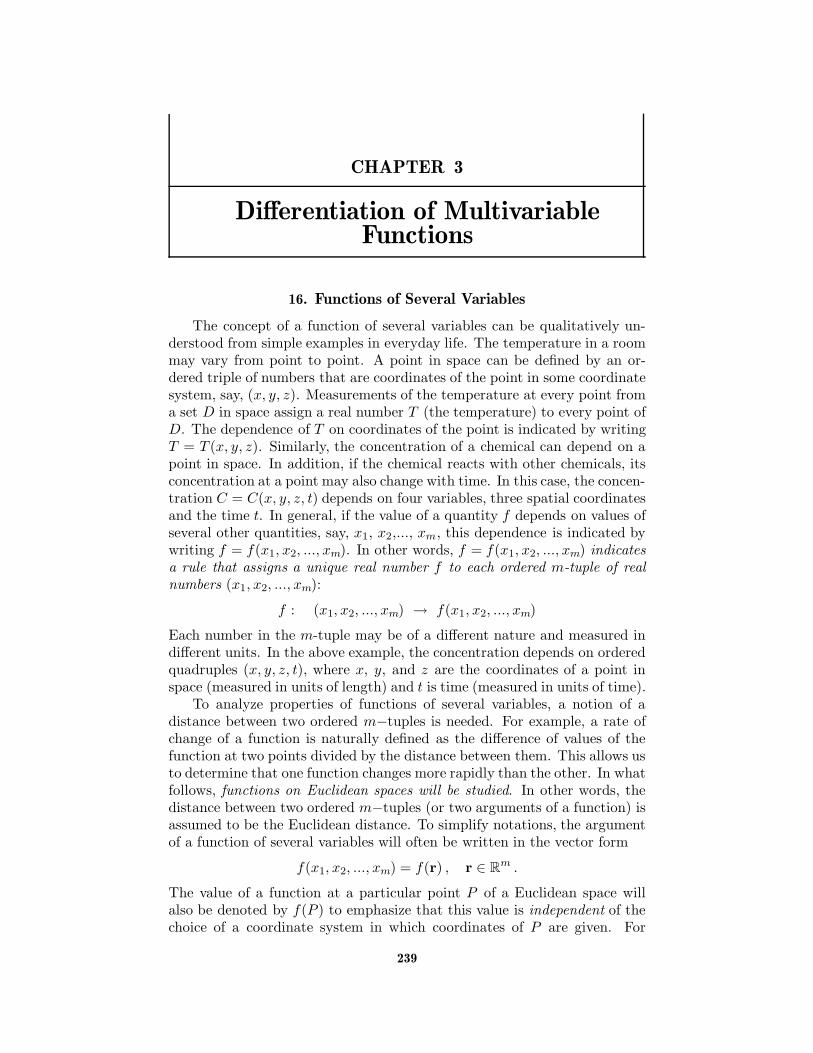
CHAPTER 3
Differentiation of MultivariableFunctions
16. Functions of Several Variables
The concept of a function of several variables can be qualitatively un-derstood from simple examples in everyday life. The temperature in a roommay vary from point to point. A point in space can be defined by an or-dered triple of numbers that are coordinates of the point in some coordinatesystem, say, (x, y, z). Measurements of the temperature at every point froma set D in space assign a real number T (the temperature) to every point ofD. The dependence of T on coordinates of the point is indicated by writingT = T (x, y, z). Similarly, the concentration of a chemical can depend on apoint in space. In addition, if the chemical reacts with other chemicals, itsconcentration at a point may also change with time. In this case, the concen-tration C = C(x, y, z, t) depends on four variables, three spatial coordinatesand the time t. In general, if the value of a quantity f depends on values ofseveral other quantities, say, x1, x2,..., xm, this dependence is indicated bywriting f = f(x1, x2, ..., xm). In other words, f = f(x1, x2, ..., xm) indicatesa rule that assigns a unique real number f to each ordered m-tuple of realnumbers (x1, x2, ..., xm):
f : (x1, x2, ..., xm) → f(x1, x2, ..., xm)
Each number in the m-tuple may be of a different nature and measured indifferent units. In the above example, the concentration depends on orderedquadruples (x, y, z, t), where x, y, and z are the coordinates of a point inspace (measured in units of length) and t is time (measured in units of time).
To analyze properties of functions of several variables, a notion of adistance between two ordered m−tuples is needed. For example, a rate ofchange of a function is naturally defined as the difference of values of thefunction at two points divided by the distance between them. This allows usto determine that one function changes more rapidly than the other. In whatfollows, functions on Euclidean spaces will be studied. In other words, thedistance between two ordered m−tuples (or two arguments of a function) isassumed to be the Euclidean distance. To simplify notations, the argumentof a function of several variables will often be written in the vector form
f(x1, x2, ..., xm) = f(r) , r ∈ Rm .
The value of a function at a particular point P of a Euclidean space willalso be denoted by f(P ) to emphasize that this value is independent of thechoice of a coordinate system in which coordinates of P are given. For
239
240 3. DIFFERENTIATION OF MULTIVARIABLE FUNCTIONS
y
x
PD f
f(P )
R f
D
P
f
f(P )
R f
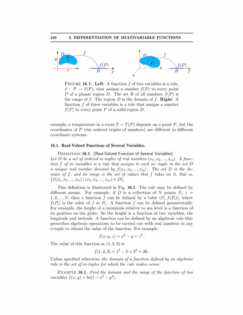
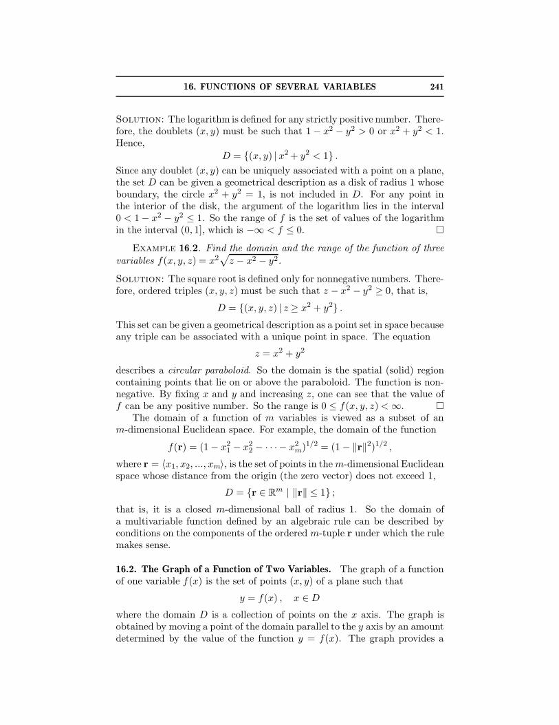
Figure 16.1. Left: A function f of two variables is a rule,f : P → f(P ), that assigns a number f(P ) to every pointP of a planar region D. The set R of all numbers f(P ) isthe range of f . The region D is the domain of f . Right: Afunction f of three variables is a rule that assigns a numberf(P ) to every point P of a solid region D.
example, a temperature in a room T = T (P ) depends on a point P , but thecoordinates of P (the ordered triples of numbers) are different in differentcoordinate systems.
16.1. Real-Valued Functions of Several Variables.
Definition 16.1. (Real-Valued Function of Several Variables).Let D be a set of ordered m-tuples of real numbers (x1, x2, ..., xm). A func-tion f of m variables is a rule that assigns to each m−tuple in the set Da unique real number denoted by f(x1, x2, ..., xm). The set D is the do-main of f , and its range is the set of values that f takes on it, that is,{f(x1, x2, ..., xm) | (x1, x2, ..., xm) ∈ D}.
This definition is illustrated in Fig. 16.1. The rule may be defined bydifferent means. For example, if D is a collection of N points Pi, i =1, 2, ..., N , then a function f can be defined by a table (Pi, f(Pi)), wheref(Pi) is the value of f at Pi. A function f can be defined geometrically.For example, the height of a mountain relative to sea level is a function ofits position on the globe. So the height is a function of two variables, thelongitude and latitude. A function can be defined by an algebraic rule thatprescribes algebraic operations to be carried out with real numbers in anyn-tuple to obtain the value of the function. For example,
f(x, y, z) = x2 − y + z3 .
The value of this function at (1, 2, 3) is
f(1, 2, 3) = 12 − 2 + 33 = 26 .
Unless specified otherwise, the domain of a function defined by an algebraicrule is the set of m-tuples for which the rule makes sense.
Example 16.1. Find the domain and the range of the function of twovariables f(x, y) = ln(1− x2 − y2).
16. FUNCTIONS OF SEVERAL VARIABLES 241
Solution: The logarithm is defined for any strictly positive number. There-fore, the doublets (x, y) must be such that 1 − x2 − y2 > 0 or x2 + y2 < 1.Hence,
D = {(x, y) | x2 + y2 < 1} .
Since any doublet (x, y) can be uniquely associated with a point on a plane,the set D can be given a geometrical description as a disk of radius 1 whoseboundary, the circle x2 + y2 = 1, is not included in D. For any point inthe interior of the disk, the argument of the logarithm lies in the interval0 < 1 − x2 − y2 ≤ 1. So the range of f is the set of values of the logarithmin the interval (0, 1], which is −∞ < f ≤ 0. �
Example 16.2. Find the domain and the range of the function of three
variables f(x, y, z) = x2√
z − x2 − y2.
Solution: The square root is defined only for nonnegative numbers. There-fore, ordered triples (x, y, z) must be such that z − x2 − y2 ≥ 0, that is,
D = {(x, y, z) | z ≥ x2 + y2} .
This set can be given a geometrical description as a point set in space becauseany triple can be associated with a unique point in space. The equation
z = x2 + y2
describes a circular paraboloid. So the domain is the spatial (solid) regioncontaining points that lie on or above the paraboloid. The function is non-negative. By fixing x and y and increasing z, one can see that the value off can be any positive number. So the range is 0 ≤ f(x, y, z) < ∞. �
The domain of a function of m variables is viewed as a subset of anm-dimensional Euclidean space. For example, the domain of the function
f(r) = (1− x21 − x2
2 − · · · − x2m)1/2 = (1 − ‖r‖2)1/2 ,
where r = 〈x1, x2, ..., xm〉, is the set of points in the m-dimensional Euclideanspace whose distance from the origin (the zero vector) does not exceed 1,
D = {r ∈ Rm | ‖r‖ ≤ 1} ;
that is, it is a closed m-dimensional ball of radius 1. So the domain ofa multivariable function defined by an algebraic rule can be described byconditions on the components of the ordered m-tuple r under which the rulemakes sense.
16.2. The Graph of a Function of Two Variables. The graph of a functionof one variable f(x) is the set of points (x, y) of a plane such that
y = f(x) , x ∈ D
where the domain D is a collection of points on the x axis. The graph isobtained by moving a point of the domain parallel to the y axis by an amountdetermined by the value of the function y = f(x). The graph provides a
242 3. DIFFERENTIATION OF MULTIVARIABLE FUNCTIONS
z
y
x
(x, y, z)z = f(x, y)
(x, y, 0)
D x
y
z
1
2 3D
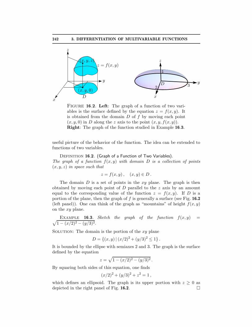
Figure 16.2. Left: The graph of a function of two vari-ables is the surface defined by the equation z = f(x, y). Itis obtained from the domain D of f by moving each point(x, y, 0) in D along the z axis to the point (x, y, f(x, y)).Right: The graph of the function studied in Example 16.3.
useful picture of the behavior of the function. The idea can be extended tofunctions of two variables.
Definition 16.2. (Graph of a Function of Two Variables).The graph of a function f(x, y) with domain D is a collection of points(x, y, z) in space such that
z = f(x, y) , (x, y) ∈ D .
The domain D is a set of points in the xy plane. The graph is thenobtained by moving each point of D parallel to the z axis by an amountequal to the corresponding value of the function z = f(x, y). If D is aportion of the plane, then the graph of f is generally a surface (see Fig. 16.2(left panel)). One can think of the graph as “mountains” of height f(x, y)on the xy plane.
Example 16.3. Sketch the graph of the function f(x, y) =√
1 − (x/2)2 − (y/3)2.
Solution: The domain is the portion of the xy plane
D = {(x, y) | (x/2)2 + (y/3)2 ≤ 1} .
It is bounded by the ellipse with semiaxes 2 and 3. The graph is the surfacedefined by the equation
z =√
1 − (x/2)2 − (y/3)2 .
By squaring both sides of this equation, one finds
(x/2)2 + (y/3)2 + z2 = 1 ,
which defines an ellipsoid. The graph is its upper portion with z ≥ 0 asdepicted in the right panel of Fig. 16.2. �
16. FUNCTIONS OF SEVERAL VARIABLES 243
z = k3z = k2z = k1
z = f(x, y)
x
y
k2k2
k3
k3
k1
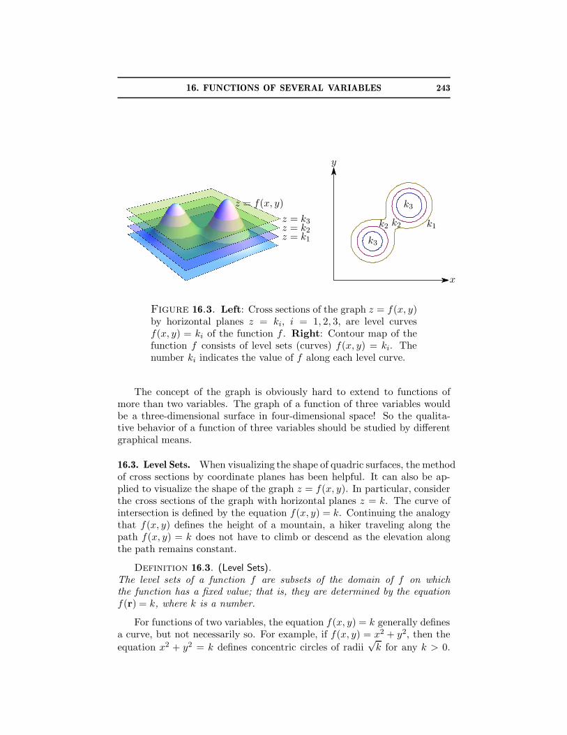
Figure 16.3. Left: Cross sections of the graph z = f(x, y)by horizontal planes z = ki, i = 1, 2, 3, are level curvesf(x, y) = ki of the function f . Right: Contour map of thefunction f consists of level sets (curves) f(x, y) = ki. Thenumber ki indicates the value of f along each level curve.
The concept of the graph is obviously hard to extend to functions ofmore than two variables. The graph of a function of three variables wouldbe a three-dimensional surface in four-dimensional space! So the qualita-tive behavior of a function of three variables should be studied by differentgraphical means.
16.3. Level Sets. When visualizing the shape of quadric surfaces, the methodof cross sections by coordinate planes has been helpful. It can also be ap-plied to visualize the shape of the graph z = f(x, y). In particular, considerthe cross sections of the graph with horizontal planes z = k. The curve ofintersection is defined by the equation f(x, y) = k. Continuing the analogythat f(x, y) defines the height of a mountain, a hiker traveling along thepath f(x, y) = k does not have to climb or descend as the elevation alongthe path remains constant.
Definition 16.3. (Level Sets).The level sets of a function f are subsets of the domain of f on whichthe function has a fixed value; that is, they are determined by the equationf(r) = k, where k is a number.
For functions of two variables, the equation f(x, y) = k generally definesa curve, but not necessarily so. For example, if f(x, y) = x2 + y2, then the
equation x2 + y2 = k defines concentric circles of radii√
k for any k > 0.
244 3. DIFFERENTIATION OF MULTIVARIABLE FUNCTIONS
However, for k = 0, the level set consists of a single point (x, y) = (0, 0).If k < 0, then the corresponding level sets are empty. Clearly, if k is notfrom the range of a function, then the corresponding level set is empty. Iff is a constant function on D, then it has just one non-empty level set; itcoincides with the entire domain D. In general, a level set of a function oftwo variables may contain curves, isolated points, and even portions of thedomain with nonzero area.
Suppose that each level set f(x, y) = k for some k in the range of f is acurve or a collection of curves. These curves are referred to as level curvesof a function. Recall that a curve in a plane can be described by parametricequations x = x(t), y = y(t) where x(t) and y(t) are continuous functionson an interval a ≤ t ≤ b. Therefore the equation f(x, y) = k defines a curve(or a collection of curves) if there exist continuous functions x(t) and y(t)(or a collection of pairs of continuous functions) such that f(x(t), y(t)) = kfor all values of t from an interval. For example, let
f(x, y) = x2 +y2
4.
Then the level set f(x, y) = 4 is an ellipse
x2 +y2
4= 4 ⇔ x2
22+
y2
42= 1
with semi-axes a = 2 and b = 4. The ellipse is also described by parametricequations
x = 2 cos t , y = 4 sin t , 0 ≤ t ≤ 2π .
Indeed, x2/22 + y2/42 = cos2 t + sin2 t = 1 for all t.
Example 16.4. Determine the level set f(x, y) = 1 of the functionf(x, y) = (3 − x2 − y2)2. If the level set contains curves, find their pa-rameterization.
Solution: It follows from the equation for the level set
(3− x2 − y2)2 = 1 ⇔ 3 − x2 − y2 = ±1 ⇔ x2 + y2 = 3 ± 1
The equations x2 + y2 = 4 and x2 + y2 = 2 describe circles of radii 2 and√2, respectively. Their parametric equations may chosen in the form
x = a cos t , y = a sin t , 0 ≤ t ≤ 2π ,
where a = 2 or a =√
2. �
Definition 16.4. (Contour Map).A collection of level curves of a function of two variables is called a contourmap of the function.
The concept of level curves and a contour map of a function of twovariables are illustrated in Fig. 16.3. The contour map of the function in
16. FUNCTIONS OF SEVERAL VARIABLES 245
Example 16.3 consists of ellipses. Indeed, the range is the interval [0, 1]. Forany 0 ≤ k < 1, a level curve is an ellipse,
1 −(x
2
)2−
(y
3
)2= k2 ⇔
(x
2
)2+
(y
3
)2= 1 − k2
or, after dividing both sides of the latter equation by k2 − 1 > 0,
x2
a2+
y2
b2= 1 , a = 2
√
1 − k2 , b = 3√
1 − k2 .
The level set for k = 1 consists of a single point, the origin. Larger values ofthe function (larger k) correspond to smaller ellipses (the semi-axes a andb decrease with increasing k). So, the contour map of the function consistsof ellipses that have a common center (the origin) and lie inside the ellipsewith a = 2 and b = 3.
A contour map is a useful tool for studying the qualitative behaviorof a function. Consider the contour map that consists of level curves Ci,i = 1, 2, ..., f(x, y) = ki, where ki+1 − ki = ∆k is fixed. The values of thefunction along the neighboring curves Ci and Ci+1 differ by ∆k. So, in theregion where the level curves are dense (close to one another), the functionf(x, y) changes rapidly. Indeed, let P be a point of Ci and let ∆s be thedistance from P to Ci+1 along the normal to Ci at P . Then the slope ofthe graph of f or the rate of change of f at P in that direction is ∆k/∆s.Thus, the closer the curves Ci are to one another, the faster the functionchanges. Contour maps are used in topography to indicate the steepness ofmountains on maps.
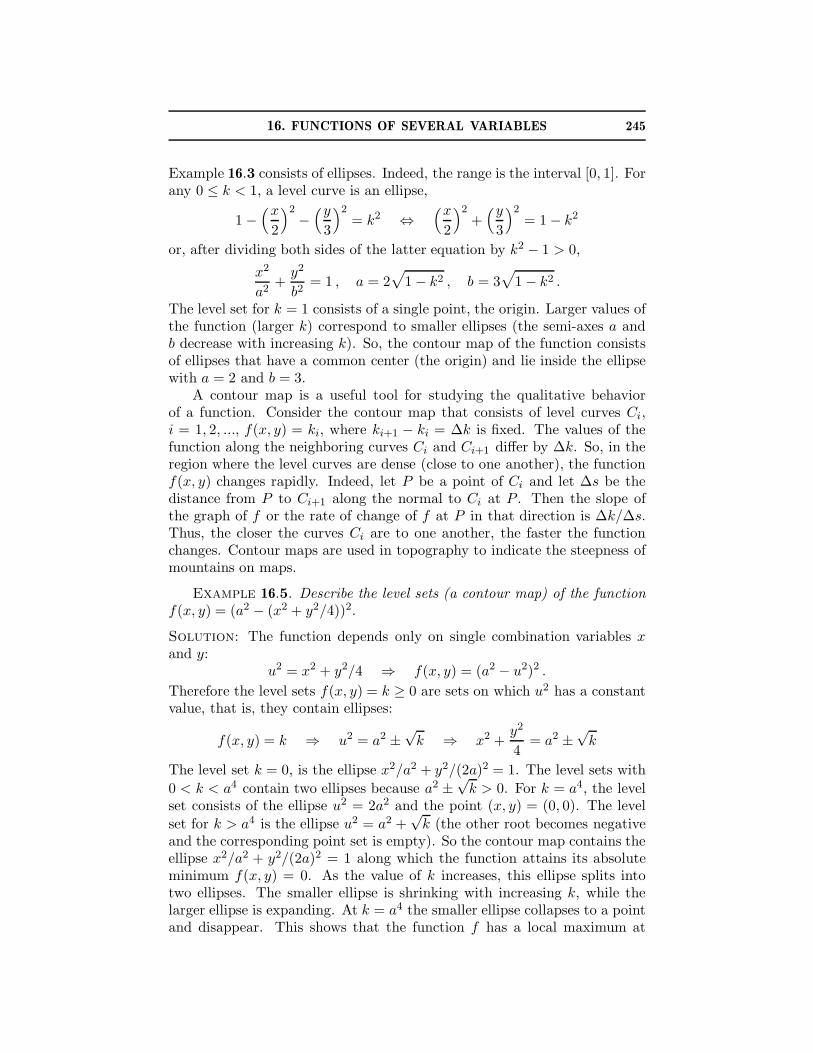
Example 16.5. Describe the level sets (a contour map) of the functionf(x, y) = (a2 − (x2 + y2/4))2.
Solution: The function depends only on single combination variables xand y:
u2 = x2 + y2/4 ⇒ f(x, y) = (a2 − u2)2 .
Therefore the level sets f(x, y) = k ≥ 0 are sets on which u2 has a constantvalue, that is, they contain ellipses:
f(x, y) = k ⇒ u2 = a2 ±√
k ⇒ x2 +y2
4= a2 ±
√k
The level set k = 0, is the ellipse x2/a2 + y2/(2a)2 = 1. The level sets with
0 < k < a4 contain two ellipses because a2 ±√
k > 0. For k = a4, the levelset consists of the ellipse u2 = 2a2 and the point (x, y) = (0, 0). The level
set for k > a4 is the ellipse u2 = a2 +√
k (the other root becomes negativeand the corresponding point set is empty). So the contour map contains theellipse x2/a2 + y2/(2a)2 = 1 along which the function attains its absoluteminimum f(x, y) = 0. As the value of k increases, this ellipse splits intotwo ellipses. The smaller ellipse is shrinking with increasing k, while thelarger ellipse is expanding. At k = a4 the smaller ellipse collapses to a pointand disappear. This shows that the function f has a local maximum at
246 3. DIFFERENTIATION OF MULTIVARIABLE FUNCTIONS
the origin, f(0, 0) = a4. The larger ellipse keeps expanding in size withincreasing k. The graph of f looks like a Mexican hat stretched along the yaxis (by a factor 2). �
16.4. Level Surfaces. In contrast to the graph, the method of level curvesuses only the domain of a function of two variables to study its behavior.Therefore the concept of level sets can be useful to study the qualitativebehavior of functions of three variables. In general, the equation f(x, y, z) =k defines a surface in space, but not necessarily so as in the case of functionsof two variables. The level sets of the function f(x, y, z) = x2 + y2 + z2 areconcentric spheres x2 +y2 +z2 = k for k > 0, the level set for k = 0 containsjust one point (the origin), and the level sets are empty for k < 0.
Intuitively, a surface in space can be obtained by a continuous deforma-tion (without breaking) of a part of a plane, just like a curve is obtainedby a continuous deformation of a line segment. Let S be a nonempty pointset in space. A neighborhood of a point P of S is a collection of all pointsof S whose distance from P is less than a number δ > 0. In particular, aneighborhood of a point in a plane is a disk centered at that point and theboundary circle does not belong to the neighborhood. If every point of asubset D of a plane has a neighborhood that is contained in D, then the setD is called open. In other words, for every point P of an open region D in aplane there is a disk of a sufficiently small radius that is centered at P andcontained in D. A point set S is a surface in space if every point of S hasa neighborhood that can be obtained by a continuous deformation (or a de-formation without breaking) of an open set in a plane and this deformationhas a continuous inverse. This is analogous to the definition of a curve as apoint set in space given in Section 10.3.
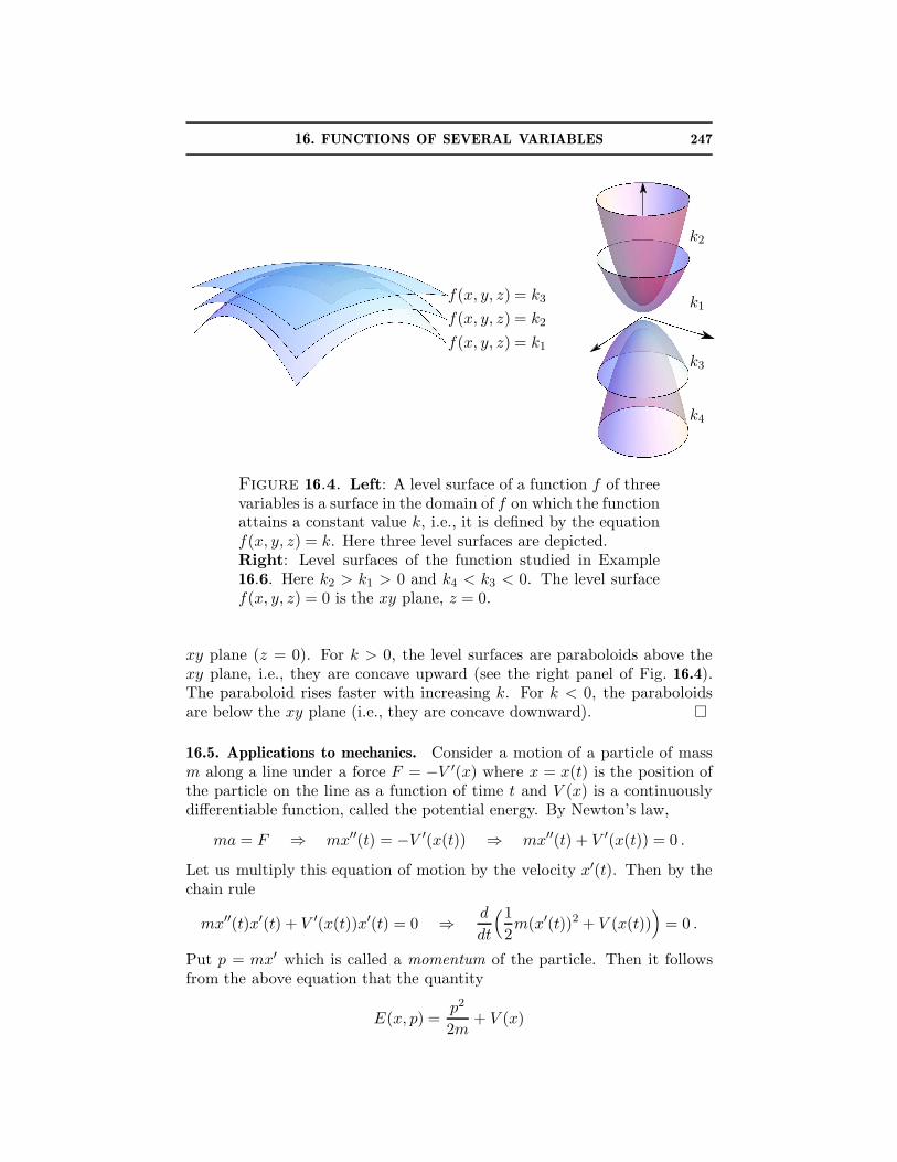
When the level sets of a function of three variables are surfaces (orcollections of surfaces), they are called level surfaces. The shape of thelevel surfaces may be studied, for example, by the method of cross sectionswith coordinate planes. A collection of level surfaces Si, f(x, y, z) = ki,ki+1 − ki = ∆k, i = 1, 2, ..., can be depicted in the domain of f . If P0 isa point on Si and P is the point on Si+1 that is the closest to P0, thenthe ratio ∆k/|P0P | determines the maximal rate of change of f at P . Sothe closer the level surfaces Si are to one another, the faster the functionchanges (see the left panel of Fig. 16.4).
Example 16.6. Sketch and/or describe the level surfaces of the functionf(x, y, z) = z/(1 + x2 + y2).
Solution: The domain is the entire space, and the range contains all realnumbers. The equation f(x, y, z) = k can be written in the form
z − k = k(x2 + y2) .
If k 6= 0, this equation defines a circular paraboloid whose symmetry axis isthe z axis and whose vertex is at (0, 0, k). For k = 0, the level surface is the
16. FUNCTIONS OF SEVERAL VARIABLES 247
f(x, y, z) = k3
f(x, y, z) = k2
f(x, y, z) = k1
k2
k1
k3
k4
Figure 16.4. Left: A level surface of a function f of threevariables is a surface in the domain of f on which the functionattains a constant value k, i.e., it is defined by the equationf(x, y, z) = k. Here three level surfaces are depicted.Right: Level surfaces of the function studied in Example16.6. Here k2 > k1 > 0 and k4 < k3 < 0. The level surfacef(x, y, z) = 0 is the xy plane, z = 0.
xy plane (z = 0). For k > 0, the level surfaces are paraboloids above thexy plane, i.e., they are concave upward (see the right panel of Fig. 16.4).The paraboloid rises faster with increasing k. For k < 0, the paraboloidsare below the xy plane (i.e., they are concave downward). �
16.5. Applications to mechanics. Consider a motion of a particle of massm along a line under a force F = −V ′(x) where x = x(t) is the position ofthe particle on the line as a function of time t and V (x) is a continuouslydifferentiable function, called the potential energy. By Newton’s law,
ma = F ⇒ mx′′(t) = −V ′(x(t)) ⇒ mx′′(t) + V ′(x(t)) = 0 .
Let us multiply this equation of motion by the velocity x′(t). Then by thechain rule
mx′′(t)x′(t) + V ′(x(t))x′(t) = 0 ⇒ d
dt
(1
2m(x′(t))2 + V (x(t))
)
= 0 .
Put p = mx′ which is called a momentum of the particle. Then it followsfrom the above equation that the quantity
E(x, p) =p2
2m+ V (x)
248 3. DIFFERENTIATION OF MULTIVARIABLE FUNCTIONS
remains constant during the motion:
d
dt
((p(t))2
2m+ V (x(t))
)
= 0 ⇒ E(x(t), p(t)) = const .
The function E(x, p) is called the total energy of the particle (the sum ofthe kinetic and potential energies). The level sets of the energy functionE(x, p) = k are called a phase space portrait of a dynamical system. Giventhe initial conditions x(0) = x0, p(0) = p0, the system evolves so that itremains in the set E(x, p) = E(x0, p0). In particular, if a level set is acurve that contain the initial state point (x0, p0), then the solution of theequation of motion (x(t), p(t)) traverses the curve E(x, p) = E(x0, p0). So,the phase space portrait describes all possible motions (for all possible initialconditions) of a given dynamical system.
For example, according to Hooke’s law, small vibrations of a mass at-tached to a spring are described by the equation
mx′′(t) = −λx(t) ,
where λ > 0 and x(t) is the coordinate of the position of the mass relative tothe equilibrium position that is set at x = 0. Since V ′(x) = λx, the potentialelastic energy is V (x) = λx2/2 (adopting the convention that the minimalvalue of the energy is set to zero, V (0) = 0). The phase space portrait ofthis dynamical system is a contour map of the energy function
E(x, p) =p2
2m+
λx2
2
It consists of ellipses, larger initial energies correspond to wider ellipses. Itfollows from the phase space portrait that the motion remains bounded forany initial conditions because for any initial energy E0:
−(2E0/λ)1/2 ≤ x(t) ≤ (2E0/λ)1/2
since (x(t), p(t)) traverses the ellipse E(x, p) = E0.
16.6. Exercises.1–13. Find and sketch the domain of each of the following functions:
1. f(x, y) = x/y .2. f(x, y) = x/(x2 + y2) .3. f(x, y) = x/(y2 − 4x2) .4. f(x, y) = ln(9 − x2 − (y/2)2) .
5. f(x, y) =√
1− (x/2)2 − (y/3)2 .
6. f(x, y) =√
4− x2 − y2 + 2x ln y .
7. f(x, y) =√
4− x2 − y2 + x ln y2 .
8. f(x, y) =√
4− x2 − y2 + ln(x2 + y2 − 1) .9. f(x, y, z) = x/(yz)
10. f(x, y, z) = x/(x− y2 − z2)11. f(x, y, z) = ln(1 − z + x2 + y2) .
16. FUNCTIONS OF SEVERAL VARIABLES 249
12. f(x, y, z) =√
x2 − y2 − z2 + ln(1− x2 − y2 − z2) .13. f(t, r) = (t2 − ‖r‖2)−1, r = 〈x1, x2, ..., xm〉 .
14–19. For each of the following functions, sketch a contour map and useit to sketch the graph:
14. f(x, y) = x2 + 4y2 .15. f(x, y) = xy .16. f(x, y) = x2 − y2 .
17. f(x, y) =√
x2 + 9y2 .18. f(x, y) = sin x .19. f(x, y) = y2 + (1 − cos x) .
20–25. Describe and sketch the level sets of each of the following functions:
20. f(x, y, z) = x + 2y + 3z .21. f(x, y, z) = x2 + 4y2 + 9z2 .22. f(x, y, z) = z + x2 + y2 .23. f(x, y, z) = x2 + y2 − z2 .24. f(x, y, z) = ln(x2 + y2 − z2) .25. f(x, y, z) = ln(z2 − x2 − y2) .
26–32. Sketch the level sets of each of the following functions. Heremin(a, b) and max(a, b) denote the smallest number and the largest numberof a and b, respectively, and min(a, a) = max(a, a) = a.
26. f(x, y) = |x| + y .27. f(x, y) = |x| + |y| − |x + y| .28. f(x, y) = min(x, y) .29. f(x, y) = max(|x|, |y|).30. f(x, y) = sign(sin(x) sin(y)); here sign(a) is the sign function, it
has the values 1 and −1 for positive and negative a, respectively.31. f(x, y, z) = (x + y)2 + z2 .
32. f(x, y) = tan−1(
2ayx2+y2−a2
)
, a > 0.
33–36. Explain how the graph z = g(x, y) can be obtained from the graphof f(x, y) if
33. g(x, y) = k + f(x, y), where k is a constant ;34. g(x, y) = mf(x, y), where m is a nonzero constant ;35. g(x, y) = f(x − a, y − b), where a and b are constants ;36. g(x, y) = f(px, qy), where p and q are nonzero constants .
37–39. Given a function f(x, y), sketch the graphs of the function g(x, y)defined in Exercises 33–36. Analyze carefully various cases for values of theconstants (for example, m > 0, m < 0, p > 1, 0 < p < 1, and p = −1, etc.)
37. f(x, y) = x2 + y2 .38. f(x, y) = xy .39. f(x, y) = (a2 − x2 − y2)2 .
250 3. DIFFERENTIATION OF MULTIVARIABLE FUNCTIONS
40. Find f(u) if f(x/y) =√
x2 + y2/x, x > 0.41. Find f(x, y) if f(x + y, y/x) = x2 − y2.42. Let z =
√y + f(
√x − 1). Find the functions z and f if z = x when
y = 1.43. Graph the function F (t) = f(cos t, sin t) where f(x, y) = 1 if y ≥ x andf(x, y) = 0 if y < x. Give a geometrical interpretation of the graph of F asan intersection of two surfaces.44–47. Let f(u) be a continuous function for all real u. Investigate therelation between the shape of the graph of f and the shape of the followingsurfaces:
44. z = f(y − ax) .
45. z = f(√
x2 + y2) .
46. z = f(−√
x2 + y2) .47. z = f(x/y) .
48. Suppose that a potential energy of a particle of mass m is V (x) =−λ(x2 − a2)2. Sketch the phase space portrait of this dynamical system intwo cases λ > 0 and λ < 0. Determine the set of all initial conditions atwhich the motion remains bounded in each case.49. A pendulum is a weight suspended on a rigid rod from a pivot sothat it can swing freely. Consider a planar motion of the pendulum. Thenits position can be described by the angle θ(t) counted counterclockwisefrom its equilibrium position as a function of time t. If L is the length ofthe pendulum and m is its mass, then its total energy is known to be E =12mL2θ2+mgL(1−cos θ) where θ = dθ/dt. Put p = mLθ (the momentum ofthe pendulum). Sketch the phase space portrait of the pendulum. Determinethe set of all initial conditions at which the pendulum cannot make a full2π turn about the pivot point.
17. LIMITS AND CONTINUITY 251
17. Limits and Continuity
The function f(x) = sin(x)/x is defined for all reals except x = 0. Sothe domain D of the function contains points arbitrarily close to the pointx = 0, and therefore the limit of f(x) can be studied as x → 0. It is knownfrom Calculus I that sin(x)/x → 1 as x → 0. A similar question can beasked for functions of several variables. For example, the domain of thefunction
f(x, y) =sin(x2 + y2)
(x2 + y2)
is the entire plane except the point (x, y) = (0, 0). The domain containspoints arbitrary close to the origin and one can compute the values of thefunction at points that are successively closer to the origin to determinewhether these values approach a particular number. For example, one cantake a straight line x = t, y = t and investigate the values of the functionon it as t → 0:
limt→0
f(t, t) = limt→0
sin(2t2)
2t2= lim
u→0
sinu
u= 1 .
In contrast to the one-dimensional case, there are infinitely many curvespassing through the origin along which the limit values of the function canbe studied. It is then natural to think of the limit, if it exists, as the numberto which the values of the function f(P ) as P approaches the origin alongany curve. It is not difficult to show that the values of the above functionindeed approach 1 along any curve through (0, 0). Let x = x(t), y = y(t)be a parametric curve through the origin such that x(0) = 0 and y(0) = 0(recall that x(t) and y(t) are continuous on an interval containing t = 0).
Then the distance from the origin R(t) =√
x2(t) + y2(t) tends to 0 as t → 0by continuity of x(t) and y(t). Therefore
limt→0
f(x(t), y(t)) = limR→0
sin(R2)
R2= 1
for any parametric curve through the point (0, 0).Consider another example: f(x, y) =
√xy. The point (1,−1) is not in
the domain of the function. Furthermore, consider a disk of a radius lessthan 1 that is centered at this point. Any such disk contains no point of thedomain of f . Evidently, the limit of f does not make any sense at (1,−1)as one cannot investigate the values of the function at points arbitrary close
to (1,−1). The domain of the function f(x, y) =√
−x2 − y2 consists ofa single point (0, 0). The limit of this function at the origin also does notmake any sense as the function has no value at any point different fromthe origin. So, first of all one has to describe points for which the veryquestion about the limit of a function makes sense. As noted before, thedomain of a function f of several variables is a point set in an n-dimensionalEuclidean space. The distance between two points x = (x1, x2, ..., xm) and
252 3. DIFFERENTIATION OF MULTIVARIABLE FUNCTIONS
y = (y1, y2, ..., ym) is the Euclidean distance
‖x− y‖ =√
(x1 − y1)2 + (x2 − y2)2 + · · ·+ (xm − ym)2 .
Definition 17.1. (Neighborhood of a Point)A neighborhood of a point r0 in a Euclidean space is an open ball of radiusδ > 0 centered at r0:
Nδ(r0) = {r | ‖r− r0‖ < δ} .
The number δ is called the radius of Nδ(r0).
In other words, a neighborhood of a point P is the collection of all pointswhose distance from P is less than some positive number. A point P mayor may not be in the domain of a function f . The limit of f at a point Pwould not make any sense if there is a neighborhood of P which contains nopoints of the domain of the function other than possibly the point P itselfbecause it would be impossible to investigate the values of the function atpoints arbitrary close to P .
Definition 17.2. (Limit Point of a Set).A point r0 is said to be a limit point of a set D if any neighborhood Nδ(r0)contains a point r of D and r 6= r0.
Let the domain of a function f be a set D. A limit point r0 of D may ormay not be in D (or f may or may not have a value at r0), but the limit ofthe function f always makes sense at a limit point of the domain D becausea neighborhood of r0 of an arbitrary small radius contains a point of D.
17.1. Limits of Functions of Several Variables. Intuitively, if the values afunction f(r) near a point r0 get arbitrary close to a number c and stayarbitrary close to c for all r 6= r0 in a suitably small neighborhood of r0,then f is said to have the limit at r0 that is equal to c.
For example, the values of f(x, y) = x3y get arbitrary close to c = 0 if x
and y are suitably small. If R = (x2 + y2)1/2 is the distance from the originto a point (x, y), then |x| ≤ R and |y| ≤ R. Therefore
|f(x, y)| = |x|3|y| ≤ R4
which shows that the values of f(x, y) stay arbitrary close to zero throughouta neighborhood of the origin of a suitably small radius, and it is concludedthat the function f(x, y) = x3y has the limit c = 0 at the point (0, 0).
Consider the function
f(x, y) =xy
x2 + y2.
The origin is not in the domain of the function, but it is a limit pointof the domain. So, one can consider the limit of this function when (x, y)approach (0, 0). The values of the function along the coordinate axes vanish,f(0, y) = f(x, 0). One can say that the values of f get arbitrary close in
17. LIMITS AND CONTINUITY 253
any neighborhood of the origin. However, they do not stay arbitrary closethroughout any neighborhood of the origin. Indeed, the values of the functionon the line y = x are equal to 1
2 = f(x, x). Evidently, 12 is not arbitrary
close to 0, but the line y = x passes through any neighborhood of the origin.Thus, it is concluded that the function considered has no limit at the origin.
The precise definition of limits. Although in the above examples it waspossible to give a precise meaning to the words “arbitrary close” and “stayarbitrary close” in a “suitably small neighborhood”, the general situationis not that simple. The precise definition of the limit is analogous to thatgiven in Calculus I for functions of a single variable.
Definition 17.3. (Limit of a Function of Several Variables).Let f be a function of several variables whose domain is a set D in a Eu-clidean space. Let r0 be a limit point of D. Then the limit of f(r) at r0
is said to be a number c if, for every number ε > 0, there exists a numberδ > 0 such that if r is in D and 0 < ‖r − r0‖ < δ, then |f(r) − c| < ε. Inthis case, one writes
limr→r0
f(r) = c or f(r) → c as r → r0
pronounced “the limit of f(r) as r approaches (or goes to) r0 is c”.
The number |f(r)−c| determines a deviation of the value of f at the pointr from the number c. So, an arbitrary positive number ε sets a numericalmeasure for how “close” the values of f to c are. The existence of the limitmeans that no matter how small the number ε is set to be, one can find aball of a sufficiently small radius δ and centered at the limit point r0 suchthat the values of the function at all points in this ball (except its center r0)deviate from the limit value c no more than ε, that is,
c − ε < f(r) < c + ε whenever 0 < ‖r− r0‖ < δ .
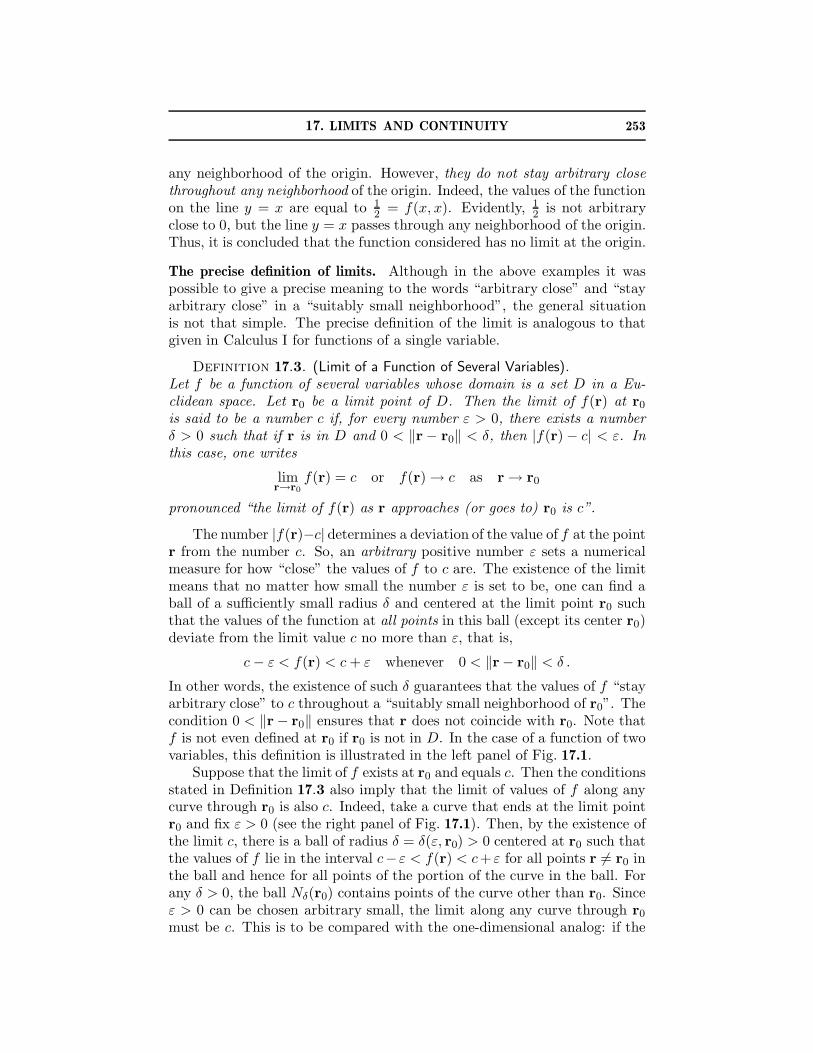
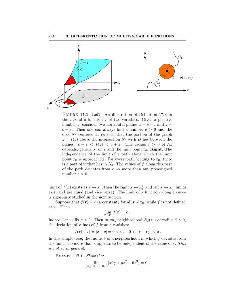
In other words, the existence of such δ guarantees that the values of f “stayarbitrary close” to c throughout a “suitably small neighborhood of r0”. Thecondition 0 < ‖r − r0‖ ensures that r does not coincide with r0. Note thatf is not even defined at r0 if r0 is not in D. In the case of a function of twovariables, this definition is illustrated in the left panel of Fig. 17.1.
Suppose that the limit of f exists at r0 and equals c. Then the conditionsstated in Definition 17.3 also imply that the limit of values of f along anycurve through r0 is also c. Indeed, take a curve that ends at the limit pointr0 and fix ε > 0 (see the right panel of Fig. 17.1). Then, by the existence ofthe limit c, there is a ball of radius δ = δ(ε, r0) > 0 centered at r0 such thatthe values of f lie in the interval c− ε < f(r) < c+ ε for all points r 6= r0 inthe ball and hence for all points of the portion of the curve in the ball. Forany δ > 0, the ball Nδ(r0) contains points of the curve other than r0. Sinceε > 0 can be chosen arbitrary small, the limit along any curve through r0
must be c. This is to be compared with the one-dimensional analog: if the
254 3. DIFFERENTIATION OF MULTIVARIABLE FUNCTIONS
z
y
x
c + ε
c
c − ε
D
δr0
y
x
C1
C2
r0
δ = δ(ε, r0)
Figure 17.1. Left: An illustration of Definition 17.3 inthe case of a function f of two variables. Given a positivenumber ε, consider two horizontal planes z = c − ε and z =c + ε. Then one can always find a number δ > 0 and thedisk Nδ centered at r0 such that the portion of the graphz = f(r) above the intersection Nδ with D lies between theplanes: c − ε < f(r) < c + ε. The radius δ > 0 of Nδ
depends, generally, on ε and the limit point r0. Right: Theindependence of the limit of a path along which the limitpoint r0 is approached. For every path leading to r0, thereis a part of it that lies in Nδ. The values of f along this partof the path deviates from c no more than any preassignednumber ε > 0.
limit of f(x) exists as x → x0, then the right x → x+0 and left x → x−
0 limitsexist and are equal (and vice versa). The limit of a function along a curveis rigorously studied in the next section.
Suppose that f(r) = c (a constant) for all r 6= r0, while f is not definedat r0. Then
limr→r0
f(r) = c .
Indeed, let us fix ε > 0. Then in any neighborhood Nδ(r0) of radius δ > 0,the deviation of values of f from c vanishes:
|f(r)− c| = |c − c| = 0 < ε , 0 < ‖r − r0‖ < δ .
In this simple case, the radius δ of a neighborhood in which f deviates fromthe limit c no more than ε appears to be independent of the value of ε. Thisis not so in general.
Example 17.1. Show that
lim(x,y,z)→(0,0,0)
(x2y + yz2 − 6z3) = 0.
17. LIMITS AND CONTINUITY 255
Solution: The distance between r = (x, y, z) and the limit point r0 =(0, 0, 0) is
R = ‖r− r0‖ =√
x2 + y2 + z2 .
Then
|x| ≤ R , |y| ≤ R , |z| ≤ R .
Let us find an upper bound on the deviation of values of the function fromthe limit value c = 0 in terms of R:
|f(r)− c| = |x2y + yz2 − 6z3| ≤ |x2y|+ |yz2| + 6|z3| ≤ 8R3,
where the inequality |a±b| ≤ |a|+ |b| and |ab| = |a||b| have been used. Nextlet us show the existence of a neighborhood of r0 with the properties statedin Definition 17.3. Fix ε > 0. To establish the existence of δ > 0, note thatthe inequality 8R3 < ε or R < 3
√ε/2 guarantees that |f(r)− c| < ε. So,
if 8R3 < ε , then |f(r)− c| < ε
Given ε > 0, one has to find a ball R < δ in which the latter inequalityholds. Therefore one can take
8δ3 = ε or δ = 3√
ε/2
so that the condition R < δ is equivalent to 8R3 < ε and, hence,
|f(r)− c| < ε whenever 0 < ‖r − r0‖ < δ = 3√
ε/2 .
For example, put ε = 10−6. Then, in the interior of a ball of radius δ = 0.005,the values of the function can deviate from c = 0 no more than 10−6. �
Note that the choice of a particular value of δ > 0 is not unique. Inthe previous example, one could take any number 0 < δ ≤ 3
√ε/2 to fulfill
the conditions for the existence of the limit. The radius δ of a neighborhoodin which a function f deviates no more than ε from the value of the limitdepends on ε and, in general, on the limit point r0, that is, δ = δ(ε, r0).
Example 17.2. Let f(x, y) = xy. Show that
lim(x,y)→(x0,y0)
f(x, y) = x0y0
for any point (x0, y0).
Solution: The distance between r = (x, y) and r0 = (x0, y0) is
R =√
(x − x0)2 + (y − y0)2 .
Therefore
|x− x0| ≤ R and |y − y0| ≤ R .
Consider the identity
xy − x0y0 = (x − x0)(y − y0) + x0(y − y0) + (x − x0)y0 .
256 3. DIFFERENTIATION OF MULTIVARIABLE FUNCTIONS
Then the deviation of f from the limit value c = x0y0 is bounded as
|f(x, y)− c| ≤ |x − x0||y − y0|+ |x0||y − y0|+ |x − x0||y0|≤ R2 + (|x0| + |y0|)R = R2 + 2aR
= (R + a)2 − a2 ,
a =1
2(|x0|+ |y0|) .
Now fix ε > 0 and demand that R is such that
0 < (R + a)2 − a2 < ε ⇒ 0 < R <√
ε + a2 − a .
Therefore the function f deviates from c = x0y0 no more than ε in a neigh-borhood of r0 of radius δ =
√ε + a2 − a:
|xy − x0y0| < ε whenever√
(x − x0)2 + (y − y0)2 < δ =√
ε + a2 − a
The radius of the neighborhood depends on ε and the limit point r0. �
17.2. An alternative definition of the limit.
Definition 17.4. A sequence of points rn, n = 1, 2, ...., in a Euclideanspace is said to converge to a point r0 if
limn→∞
‖r0 − rn‖ = 0
or, for any ε > 0 there exists an integer N such that
‖r0 − rn‖ < ε for all n > N
In this case, rn is also said to approach r0 as n → ∞ and one writeslimn→∞ rn = r0 or rn → r0 as n → ∞.
In other words, a sequence of points approaches a particular point ifthe distance between the particular point and the points of the sequencetends to zero. One can also say that only finitely many points (n ≤ N ) ofa convergent sequence are outside of any neighborhood Nε(r0) of the limitpoint.
As noted in the beginning of this section, for functions of several vari-ables, there are infinitely many ways of how the limit point can be ap-proached from within the domain of the function. More precisely, there areinfinitely many sequences of points approaching the same limit point. Onecan take values of the function f(rn) on each such sequence and investigatethe limit of the numerical sequence f(rn). The question of interest is: Whatis the relation between the limit of the function at a limit point and thelimits of the values of the function on various sequences of points convergingto the limit point? The following theorem answers this question.
Theorem 17.1. Let r0 be a limit point of the domain D of a functionf . Then
limr→r0
f(r) = c if and only if limn→∞
f(rn) = c
for every sequence of points rn in D that converges to r0 and rn 6= r0.
17. LIMITS AND CONTINUITY 257
Proof. Suppose that limr→r0f(r) = c. Choose a sequence of points rn
that converges to r0. Fix ε > 0. By Definition 17.3 there is δ > 0 such that|f(r)− c| < ε whenever 0 < ‖r − r0‖ < δ. By Definition 17.4, for any suchnumber δ > 0 there also exists an integer N such that 0 < ‖rn − r0‖ < δ forall n > N . Therefore
|f(rn)− c| < ε for all n > N
which means that the numerical sequence of values of the function f(rn)converges to the number c.
Conversely, suppose that the numerical sequence of values of the functionf(rn) converges to c for every sequence of points rn 6= r0 that converges tothe point r0. One has to show that limr→r0
f(r) = c. Suppose that thisconclusion is false. Then by negating Definition 17.3 there should existsome ε > 0 such that for every δ > 0 one can find a point r in D (dependingon δ) for which
|f(r)− c| ≥ ε but 0 < ‖r− r0‖ < δ .
Since this property should be true for any δ, it is true if δ = δn = 1/n, wheren = 1, 2, 3, .... For each δn there is a point r = rn with the above property.This means that there is a sequence of points rn approaching r0 because‖rn − r0‖ < 1/n → 0 as n → ∞, but the corresponding sequence of valuesof the function f(rn) does not converge to c. This is a contradiction. So,limr→r0
f(r) = c. �
The intuitive idea that the limit of a function, if it exists, should notdepend on the way the limit point is approached is now rigorously establishedin Theorem 17.1. The conditions under which the limit exists stated inDefinition 17.3 and in Theorem 17.1 have been proved to be equivalent. SoTheorem 17.1 could have been used as a definition of the limit of a functionof several variables: the limit of a function f exists at a limit point r0 of thedomain of f and equals c if the limit of the numerical sequence of values off on every sequence of points not containing r0 and converging to r0 existsand equals c. Then Definition 17.3 becomes a theorem to be proved in thisapproach.
17.3. Properties of the Limit. The basic properties of limits of functionsof one variable discussed in Calculus I are extended to the case of functionsof several variables.
Theorem 17.2. (Properties of the Limit).Let f and g be functions of several variables that have a common domain.Let c be a number. Suppose that limr→r0
f(r) = p and limr→r0g(r) = q.
258 3. DIFFERENTIATION OF MULTIVARIABLE FUNCTIONS
Then the following properties hold:
limr→r0
(cf(r)) = c limr→r0
f(r) = cp,
limr→r0
(g(r) + f(r)) = limr→r0
g(r) + limr→r0
f(r) = q + p,
limr→r0
(g(r)f(r)) = limr→r0
g(r) limr→r0
f(r) = qp,
limr→r0
g(r)
f(r)=
limr→r0g(r)
limr→r0f(r)
=q
p, if p 6= 0.
A proof of Theorem 17.2 is left to the reader as an exercise. As ahint, note that, by Theorem 17.1, the above properties of the limit can beequivalently restated in terms of the basic limits laws for numerical sequenceswhich have been established in Calculus II.
Squeeze Principle. The solution to Example 17.1 employs a rather generalstrategy to verify whether a particular number c is the limit of f(r) asr → r0.
Theorem 17.3. (Squeeze Principle).Let the functions of several variables g, f , and h have a common domainD and g(r) ≤ f(r) ≤ h(r) for any r ∈ D. If the limits of g(r) and h(r) asr → r0 exist and equal a number c, then the limit of f(r) as r → r0 existsand equals c, that is,
g(r) ≤ f(r) ≤ h(r) and limr→r0
g(r) = limr→r0
h(r) = c ⇒ limr→r0
f(r) = c.
Proof. From the hypothesis of the theorem, it follows that
0 ≤ f(r)− g(r) ≤ h(r) − g(r) .
PutF (r) = f(r)− g(r) , H(r) = h(r)− g(r) .
Then0 ≤ F (r) ≤ H(r)
implies |F (r)| ≤ |H(r)| (the positivity of F is essential for this conclusion).By the hypothesis of the theorem and the properties of the limit,
H(r) = h(r)− g(r) → c− c = 0 as r → r0 .
Hence, for any ε > 0, there is a number δ such that
0 ≤ |F (r)| ≤ |H(r)| < ε whenever 0 < ‖r− r0‖ < δ .
By Definition 17.3 this means that limr→r0F (r) = 0. By the basic properties
of the limit, it is then concluded that
f(r) = F (r) + g(r) → 0 + c = c as r → r0 .
�
Alternatively, the squeeze principle for limits of functions can be estab-lished from the squeeze principle for numerical sequences by using Theorem
17. LIMITS AND CONTINUITY 259
17.1. The details are left to the reader as an exercise. A particular case ofthe squeeze principle is also useful.
Corollary 17.1. (Simplified Squeeze Principle).If there exists a function h of one variable such that
|f(r)− c| ≤ h(R) → 0 as ‖r− r0‖ = R → 0+,
then limr→r0f(r) = c.
The condition |f(r)− c| ≤ h(R) is equivalent to
c − h(R) ≤ f(r) ≤ c + h(R)
which is a particular case of the hypothesis in the squeeze principle. InExample 17.1, h(R) = 8R3. In general, the condition h(R) → 0 as R → 0+
implies that, for any ε > 0, there is an interval 0 < R < δ(ε) in whichh(R) < ε, where the number δ can be found by solving the equation h(δ) = ε.Hence, |f(r)− c| < ε whenever ‖r− r0‖ = R < δ(ε).
Example 17.3. Show that
lim(x,y)→(0,0)
f(x, y) = 0, where f(x, y) =x3y − 3x2y2
x2 + y2 + x4.
Solution: Let R =√
x2 + y2 (the distance from the limit point (0, 0)).Then |x| ≤ R and |y| ≤ R. Therefore,
|x3y − 3x2y2|x2 + y2 + x4
≤ |x|3|y|+ 3x2y2
x2 + y2 + x4≤ 4R4
R2 + x4=
4R2
1 + (x4/R2)≤ 4R2 .
It follows from this inequality that
−4(x2 + y2) ≤ f(x, y) ≤ 4(x2 + y2) ,
and, by the squeeze principle, f(x, y) must tend to 0 because±4(x2 + y2) = ±4R2 → 0 as R → 0. In Definition 17.3, given ε > 0, anumber δ may be chosen as
√ε/2 (or smaller). �
17.4. Continuity of Functions of Several Variables. Continuous functionsof several variables are defined by analogy with continuous functions of asingle variable.
Definition 17.5. (Continuity).A function f of several variables with domain D is said to be continuous ata point r0 in D if
limr→r0
f(r) = f(r0) .
The function f is said to be continuous on D if it is continuous at everypoint of D.
Example 17.4. Let f(x, y) = 1 if y ≥ x and let f(x, y) = 0 if y < x.Determine the region on which f is continuous.
260 3. DIFFERENTIATION OF MULTIVARIABLE FUNCTIONS
Solution: The function is continuous at every point (x0, y0) if y0 6= x0.Indeed, if y0 > x0, then f(x0, y0) = 1. On the other hand, for every suchpoint one can find a disk of a sufficiently small radius δ and centered at(x0, y0)) that lies in the region y > x. Therefore, for any ε > 0,
|f(r)− f(r0)| = 1 − 1 = 0 < ε whenever (x − x0)2 + (y − y0)
2 < δ2 ,
which means that limr→r0f(r) = f(r0) = 1. The same line of reasoning
applies to establish the continuity of f at any point (x0, y0), where y0 < x0.If r0 = (x0, x0), that is, the point lies on the line y = x, then f(r0) = 1.
Any disk centered at such r0 is split into two parts by the line y = x. Inone part (y ≥ x), f(r) = 1, whereas in the other part (y < x), f(r) = 0.So, for 0 < ε < 1, there is no disk of radius δ > 0 in which |f(r)− f(r0)| =|f(r)−1| < ε because |f(r)−1| = 1 for y < x in any such disk. The functionis not continuous along the line y = x in its domain. �
Discontinuity at a limit point. Suppose that limr→r0f(r) = c. If the limit
point r0 lies in the domain of the function f , then the function has a valuef(r0) and this value may or may not coincide with the limit value c. In fact,the limit value c does not generally give any information about the possiblevalue of the function at the limit point. For example, if f(r) = 1 everywhereexcept one point r0 at which f(r0) = f0. Then in every neighborhood0 < ‖r − r0‖ < δ, f(r) = 1 and, hence, the limit of f as r → r0 exists andequals c = 1. When f0 6= 1, the limit value does not coincide with the valueof the function at the limit point. The values of f suffer a jump discontinuitywhen r reaches r0, and one says that f is discontinuous at r0.
A discontinuity also occurs when the limit of f as r → r0 does not existwhile f has a value at the limit point. Furthermore, if r0 is a limit pointof the domain D of f , but is not in D, then f is continuously extendableto a larger domain D ∪ {r0} (the union of D and the point r0) if the limitlimr→r0
f(r) exists (the function is defined at r0 by its limit value at r0). Afunction f is said to be discontinuous at a limit point r0 of its domain D if
(i) limr→r0f(r) does not exist, or
(ii) limr→r0f(r) exists, and r0 is in D, but limr→r0
f(r) 6= f(r0).
Note that the notion of “discontinuity at a limit point” of a function doesnot always mean that the function is not continuous at a limit point becausethe limit point may not be in the domain of the function (the function hasno value at that point). It means that the function is either not continuousat a limit point (if the limit point is in the domain) or not continuouslyextendable to the limit point (if the limit point is not in the domain). Forexample, one says that the function f(x) = 1/x is discontinuous at x = 0.Strictly speaking, this function is continuous on its domain (all x 6= 0).Therefore one can also say that f is a continuous function of x that isdiscontinuous at x = 0! This terminological paradox is eliminated if onekeeps in mind that, in this case, the term “discontinuous at x = 0” refers to
17. LIMITS AND CONTINUITY 261
the fact that f(x) is not continuously extendable to the limit point x = 0 ofits domain. The function g(x) = x2/x is also not defined at x = 0 (the rulemakes no sense at x = 0). But it can be continuously extended to x = 0 byg(0) = 0 and therefore has no discontinuity at x = 0.
17.5. Properties of continuous functions. The following theorem is a simpleconsequence of the basic properties of the limit.
Theorem 17.4. (Properties of Continuous Functions).If f and g are continuous on D and q is a number, then qf(r), f(r) + g(r),and f(r)g(r) are continuous on D, and f(r)/g(r) is continuous at any pointon D for which g(r) 6= 0.
The use of the definition to establish the continuity of a function definedby an algebraic rule is not always convenient. The following two theoremsare helpful when studying the continuity of a given function. For an orderedm-tuple r = 〈x1, x2, ..., xm〉, the function
f(r) = xk1
1 xk2
2 · · ·xkmm ,
where k1, k2, ..., km are nonnegative integers, is called a monomial of degreeN = k1 +k2 + · · ·+km. For example, for two variables, monomials of degreeN = 3 are
x3 , x2y , xy2 , y3 .
A function f that is a linear combination of monomials is called a polynomialfunction. For example, the function
f(x, y, z) = 1 + y − 2xz + z4
is a polynomial of three variables. The ratio of two polynomial functions iscalled a rational function.
Theorem 17.5. (Continuity of Polynomial and Rational Functions).Let f and g be polynomial functions of several variables. Then they arecontinuous everywhere, and the rational function f(r)/g(r) is continuous atany point r0 if g(r0) 6= 0.
Proof. Let f(r) = c be a constant function. Take a sequence of pointsrn converging to r0 and rn 6= r0. Then the numerical sequence f(rn) = cconverges to c. By Theorem 17.1, f(r) → c = f(r0) as r → r0. So, a con-stant function is continuous everywhere. Let gj(r) = xj (the jth coordinateof a point r). Let r0 = 〈a1, a2, ..., am〉. Since |xj − aj| ≤ ‖r − r0‖ = R, thefunction gj is continuous everywhere by the squeeze principle:
|gj(r)− gj(r0)| = |xj − aj| ≤ R → 0 as R → 0+ .
A monomial of any degree is a product of the functions gj, j = 1, 2, ..., m,or a constant function. By the properties of continuous functions (Theorem17.4), any monomial is a function continuous everywhere. A polynomial is alinear combination of monomials and therefore is also a function continuous
262 3. DIFFERENTIATION OF MULTIVARIABLE FUNCTIONS
everywhere. A rational function is continuous as the ratio of two continuousfunctions (provided the denominator does not vanish). �
Theorem 17.6. (Continuity of a Composition).Let g(u) be continuous on the interval u ∈ [a, b] and let h be a functionof several variables that is continuous on D and has the range [a, b]. Thecomposition f(r) = g(h(r)) is continuous on D.
This theorem follows from Theorem 17.1 and Definition 17.5. A proofis left to the reader as an exercise.
Basic functions studied in Calculus I, sinu, cosu, eu, ln u, and so on,are continuous functions on their domains. If f(r) is a continuous functionof several variables, the elementary functions whose argument is replacedby f(r) are continuous functions. In combination with the properties ofcontinuous functions, the composition rule defines a large class of contin-uous functions of several variables, which is sufficient for many practicalapplications.
Example 17.5. Find the limit
limr→0
exz cos(xy + z2)
x + yz + 3xz4 + (xyz − 2)2
Solution: The function is a ratio. The denominator is a polynomial andhence continuous. Its limit value is (−2)2 = 4 6= 0. The function exz isa composition of the exponential eu and the polynomial u = xy. So itis continuous. Its value is 1 at the limit point. Similarly, cos(xy + z2) iscontinuous as a composition of cosu and the polynomial u = xy + z2. Itsvalue is 1 at the limit point. The ratio of continuous functions is continuousand the limit is 1/4. �
17.6. Study Problems.
Problem 17.1. Consider two rational functions f(x, y) = x2/(x2+y2) andg(x, y) = x4/(x2 +y2). Find all points of discontinuity of these functions, ifany.
Solution: The denominator x2 + y2 vanishes only at the origin (0, 0).Therefore f and g are continuous everywhere but the origin (Theorem 17.5).The origin is not in the domain of these function but it is a limit point of thedomain. Let us verify whether these function are continuously extendable
to the whole plane. Since |x| ≤√
x2 + y2 = R, by the squeeze principle
|g(x, y)|= x4
R2≤ R4
R2= R2 → 0 as R → 0+
it is concluded that g(x, y) → 0 as (x, y) → (0, 0). So, g has no discontinuityat the origin (it is continuously extendable to the whole plane by g(0, 0) = 0).

17. LIMITS AND CONTINUITY 263
Take a sequence of points (xn, 0) where xn → 0 and as n → ∞ and xn 6= 0(it converges to the origin from within the domain of f). Then
limn→0
f(xn, 0) = limn→∞
x2n
x2n
= 1 .
On the other hand, for a sequence of points (0, yn) where yn → 0 and asn → ∞ and yn 6= 0 (it also converges to the origin from within the domainof f), a different limit value of f is obtained:
limn→0
f(0, yn) = limn→∞
0
y2n
= 0 .
By Theorem 17.1, the limit of f(x, y) at (0, 0) does not exists and f isdiscontinuous at the limit point (0, 0) of its domain (it is not continuouslyextendable to the whole plane). �
17.7. Exercises.1–5. Use Definition 17.3 of the limit to verify each of the following limits(i.e., given ε > 0, find a neighborhood of the limit point with the properiesspecified in the definition):
1. limr→0
x3 − 4y2x + 5y3
x2 + y2= 0
2. limr→0
x3 − 4y2x + 5y3
3x2 + 4y2= 0
3. limr→0
x3 − 4y4 + 5y3x2
3x2 + 4y2= 0
4. limr→0
x3 − 4y2x + 5y3
3x2 + 4y2 + y4= 0
5. limr→0
3x3 + 4y4 − 5z5
x2 + y2 + z2= 0
6–8. Use the squeeze principle to prove the following limits and find aneighborhood of the limit point in which the deviation of the function fromthe limit value does not exceed a small given number ε (Hint: | sinu| ≤ |u|):
6. limr→0
y sin(x/√
y) = 0
7. limr→0
[1 − cos(y/x)]x2 = 0
8. limr→0
cos(xy) sin(4x√
y)√
xy= 0
9. Suppose that limr→r0f(r) = 2 and r0 is in the domain of f . If nothing
else is known about the function, what can be said about the value f(r0)?If, in addition, f is known to be continuous at r0, what can be said aboutthe value f(r0)?10–19. Find the points of discontinuity of each of the following functions:
264 3. DIFFERENTIATION OF MULTIVARIABLE FUNCTIONS
10. f(x, y) = yx/(x2 + y2) ;11. f(x, y, z) = yxz/(x2 + y2 + z2) ;12. f(x, y) = sin(
√xy) ;
13. f(x, y) = cos(√
xyz)/(x2y2 + 1) ;
14. f(x, y) = (x2 + y2) ln(x2 + y2) ;15. f(x, y) = 1 if either x or y is rational and f(x, y) = 0 elsewhere. ;16. f(x, y) = (x2 − y2)/(x− y) if x 6= y and f(x, x) = 2x ;17. f(x, y) = (x2 − y2)/(x− y) if x 6= y and f(x, x) = x ;18. f(x, y, z) = 1/[sin(x) sin(z − y)] ;
19. f(x, y) = sin(
1xy
)
.
20–22. Each of the following functions has the value at the origin f(0, 0) =c. Determine whether there is a particular value of c at which the functionis continuous at the origin if for (x, y) 6= (0, 0):
20. f(x, y) = sin(
1/(x2 + y2))
;
21. f(x, y) = (x2 + y2)ν sin(
1/(x2 + y2))
, ν > 0 ;
22. f(x, y) = xnym sin(
1/(x2 + y2))
, n ≥ 0, m ≥ 0, and n + m > 0 .
23-27. Use the properties of continuous functions to find the following limits
23. limr→0
(1 + x + yz2)1/3
2 + 3x − 4y + 5z2
24. limr→0
sin(x√
y)
25. limr→0
sin(x√
y)
cos(x2y)
26. limr→0
[exyz − 2 cos(yz) + 3 sin(xy)]
27. limr→0
ln(1 + x2 + y2z2)
28. Use Theorem 17.1 and the properties of limits of numerical sequencesto prove Theorem 17.2.29. Use Theorem 17.1 to prove Theorem 17.6.
18. A GENERAL STRATEGY TO STUDY LIMITS 265
18. A General Strategy to Study Limits
The definition of the limit gives only the criterion for whether a numberc is the limit of f(r) as r → r0. In practice, however, a possible value of thelimit is typically unknown. Some studies are needed to make an “educated”guess for a possible value of the limit. Here a procedure to study limits isoutlined that might be helpful. In what follows, the limit point is often set tothe origin r0 = 0. This is not a limitation because one can always translatethe origin of the coordinate system to any particular point by shifting thevalues of the argument, for example,
lim(x,y)→(x0,y0)
f(x, y) = lim(x,y)→(0,0)
f(x + x0, y + y0) ,
or, in general,
limr→r0
f(r) = limr→0
f(r + r0) .
18.1. Step 1: Continuity Argument. The simplest scenario in studying thelimit happens when the function f in question is continuous at the limitpoint:
limr→r0
f(r) = f(r0) .
For example,
lim(x,y)→(1,2)
xy
x3 − y2= −2
3
because the function in question is a rational function that is continuous ifx3 − y2 6= 0. The latter is indeed the case for the limit point (1, 2). If thecontinuity argument does not apply, then it is helpful to check the following.
18.2. Step 2: Composition Rule.
Theorem 18.1. (Composition Rule for Limits).Let g(t) be a function continuous at t0. Suppose that the function f is thecomposition f(r) = g(h(r)) so that r0 is a limit point of the domain of fand h(r) → t0 as r → r0. Then
limr→r0
f(r) = limt→t0
g(t) = g(t0).
The proof is omitted as it is similar to the proof of the composition rulefor limits of single-variable functions given in Calculus I. The significance ofthis theorem is that, under the hypotheses of the theorem, a tough problemof studying a multivariable limit is reduced to the problem of the limit ofa function of a single argument. The latter problem can be studied, by, forexample, analyzing a local behavior of the function by a Taylor polynomialapproximation or by l’Hospital’s rule. Although there is a generalization ofl’Hospital’s rule for multivariable limits, but it is far more complicated andmuch less practical to use as compared with the one-variable case. Variousasymptotic approximations of the behavior of functions involved near the
266 3. DIFFERENTIATION OF MULTIVARIABLE FUNCTIONS
limit point such as, e.g., Taylor polynomial approximations, are much morepractical to study multivariable limits.
Example 18.1. Find
lim(x,y)→(0,0)
cos(xy)− 1
x2y2.
Solution: The function in question is g(t) = (cos t−1)/t2 for t 6= 0, wherethe argument t is replaced by the function h(x, y) = xy. The function h isa polynomial and hence continuous. In particular, h(x, y) → h(0, 0) = 0 as(x, y) → (0, 0). The function g(t) is continuous for all t 6= 0 and its value att = 0 is not defined. Since cos t = 1− t2/2 + O(t4) for small t,
limt→0
cos t − 1
t2= lim
t→0
−t2/2 + O(t4)
t2= lim
t→0
(
−1
2+ O(t2)
)
= −1
2.
So the function g(t) is continuously extendable at t = 0. By setting g(0) =−1/2, the function g(t) becomes continuous at t = 0 and the hypotheses ofthe composition rule are fulfilled. Therefore the two dimensional limit inquestion exists and equals −1/2. �
18.3. Step 3: Limits Along Curves. Recall the following result about thelimit of a function of one variable. The limit of f(x) as x → x0 exists andequals c if and only if the corresponding right and left limits of f(x) existand equal c:
limx→x+
0
f(x) = limx→x−
0
f(x) = c ⇐⇒ limx→x0
f(x) = c .
In other words, if the limit exists, it does not depend on the direction fromwhich the limit point is approached. Consequently, this fact allows us tostate a useful criterion for non-existence of the limit. If the left and rightlimits exist but do not coincide, or at least one of them does not exist,then the limit does not exist. A similar criterion for non-existence of amultivariable limit can be found.
Definition 18.1. (Parametric Curve in a Euclidean Space).A parametric curve in a Euclidean space R
m is a continuous vector functionr(t) = 〈x1(t), x2(t), ..., xm(t)〉, where t ∈ [a, b].
This is a natural generalization of the concept of a parametric curve ina plane or space defined by parametric equations xi = xi(t), i = 1, 2, ..., m,where xi(t) are continuous functions on [a, b]. For example, the parametriccurve r(t) = vt, ‖v‖ 6= 0, is the line through the origin parallel to the vectorv. (or a part of this line if the range of the parameter t is restricted to aninterval [a, b]).
Definition 18.2. (Limit Along a Curve).Let r0 be a limit point of the domain D of a function f . Suppose there isa parametric curve r(t), t0 ≤ t ≤ b, such that r(t) is in D if t > t0 and
18. A GENERAL STRATEGY TO STUDY LIMITS 267
r(t0) = r0. Let F (t) = f(r(t)), t > t0, be the values of f on the curve. Thelimit
limt→t+0
F (t) = limt→t+0
f(x1(t), x2(t), ..., xm(t))
is called the limit of f along the curve r(t) if it exists.
Theorem 18.2. If the limit of f(r) exists as r → r0 and is equal to c,then the limit of f along any curve through r0 exists and is equal to c .
Proof. Fix ε > 0. By Definition 17.3 the existence of the limit c of f(r)at r0 means that one can find a number δ > 0 such that
|f(r)− c| < ε whenever 0 < ‖r − r0‖ < δ
The vector function r(t) is continuous at t0, that is, limt→t+0
r(t) = r(t0) = r0
by the hypothesis. It follows then from Definition 10.2 of the limit of a vectorfunction that for the number δ found above there is a number δ′ > 0 suchthat
‖r(t)− r0‖ < δ whenever t0 < t < t + δ′ .
These two relations imply that for any number ε > 0 one can find a numberδ′ such that
|f(r(t))− c| = |F (t) − c| < ε whenever t0 < t < t + δ′ .
By the definition of the one-variable limit (Calculus I), this means thatF (t) → c as t → t+0 . So, the limit along any curve exists and is equal to c.�
In regard of this theorem, recall the discussion of the right panel inFig. 17.1 in Section 17.1. An immediate consequence of this theorem is auseful criterion for non-existence of a multi-variable limit.
Corollary 18.1. (Criterion for Nonexistence of the Limit).Let f be a function of several variables on D and r0 be a limit point ofD. If there is a curve along which the limit of f at r0 does not exist, thenthe multivariable limit limr→r0
f(r) does not exist either. If there are twocurves along which the limits of f at r0 exist but do not coincide, then themultivariable limit limr→r0
f(r) does not exist.
Repeated limits. Let (x, y) 6= (0, 0). Consider a curve C1 that consistsof two straight line segments (x, y) → (x, 0) → (0, 0) and a curve C2 thatconsists of two straight line segments (x, y) → (0, y) → (0, 0). Both thecurves connect (x, y) with the origin. The limits along C1 and C2,
limy→0
(
limx→0
f(x, y))
and limx→0
(
limy→0
f(x, y))
are called the repeated limits. Suppose that all points of C1 and C2 arewithin the domain of f except the point (0, 0). Then Theorem 18.2 andCorollary 18.1 establish the relations between the repeated limits and the
268 3. DIFFERENTIATION OF MULTIVARIABLE FUNCTIONS
two-variable limit lim(x,y)→(0,0) f(x, y). In particular, suppose that the func-tion is continuous with respect to x if y 6= 0 is fixed and it is also continuouswith respect to y if x 6= 0 is fixed. Then f(x, y) → f(0, y) as x → 0 for y 6= 0and f(x, y) → f(x, 0) as y → 0 for x 6= 0. The repeated limits become
limy→0
f(0, y) and limx→0
f(x, 0)
If at least one of them does not exists or they exist but are not equal, thenby Corollary 18.1 the two-variable limit does not exist. If they exist andare equal, then the two-variable limit may or may not exist. A furtherinvestigation of the two-variable limit is needed.
Example 18.2. Find the limit
lim(x,y)→(0,0)
sin(x2 − y2)
x2 + y2
or show that the limit does not exist.
Solution: The domain of the function in question is the entire plane withorigin removed. The function is continuous with respect to x if y 6= 0 isfixed and with respect to y if x 6= 0 is fixed. Therefore the repeated limitsare
limy→0
(
limx→0
sin(x2 − y2)
x2 + y2
)
= limy→0
sin(−y2)
y2= − lim
y→0
sin(y2)
y2= −1
limx→0
(
limy→0
sin(x2 − y2)
x2 + y2
)
= limx→0
sin(x2)
x2= 1
The repeated limits exist but do not coincide. Therefore the two-variablelimit does not exist. �
The following should be emphasized. Suppose that the domain of thefunction f does not include the coordinate axes (or their parts with theorigin), but the coordinates axes consist of limit points of the domain (e.g.,the domain of f contains points (x, y) with x > 0 and y > 0). Then therepeated limits make sense. However, the hypotheses of Corollary 18.1 arenot fulfilled (the curves along which the limits are taken are not in thedomain of the function). Examples given in Exercises 1-3 illustrate thesituation in this case. In particular, the non-existence of the repeated limitsdoes not imply the non-existence of the two-variable limit in this case. Anexample is given in Exercise 3.
Limits Along Straight Lines. Let the limit point be the origin r0 = 0. Thesimplest curve through r0 is a straight line xi = vit, where t → 0+ for somenumbers vi, i = 1, 2, ...,m, that do not vanish simultaneously (or in thevector form r(t) = tv, v 6= 0). In particular, in the case of two variables itis convenient to take
x = t , y = at or x = t cos θ , y = t sin θ

18. A GENERAL STRATEGY TO STUDY LIMITS 269
where a and θ are parameters. If the multivariable limit of f exists, thenthe limit of f along every straight line (in the domain of f) should exist andbe the same:
limr→0
f(r) = c ⇒ limt→0+
f(tv) = c for any v 6= 0 .
Consequently, if the limit along a particular line does not exists, or thereare two lines along which the limits exist but are not equal, then the multi-variable limit does not exist:
limt→0+ f(tv) does not existorlimt→0+ f(tv1) 6= limt→0+ f(tv2)
⇒ limr→0
f(r) does not exist
where v1 and v2 are not parallel (v1 6= sv2, s > 0).
Example 18.3. Investigate the two-variable limit
lim(x,y)→(0,0)
xy3
x4 + 2y4.
Solution: Consider the limits along straight lines x = t, y = at (or y = ax,where a is the slope) as t → 0+:
limt→0+
f(t, at) = limt→0+
a3t4
t4(1 + 2a4)=
a3
1 + 2a4.
So the limit along a straight line depends on the slope of the line. Therefore,the two-variable limit does not exist. �
Example 18.4. Investigate the limit
lim(x,y)→(0,0)
sin(√
xy)
x + y.
Solution: The domain of the function consists of the first and third quad-rants as xy ≥ 0 except the origin. Lines approaching (0, 0) from within thedomain are x = t, y = at, a ≥ 0 and t → 0. The line x = 0, y = t also liesin the domain (the line with an infinite slope). The limit along a straightline approaching the origin from within the first quadrant is
limt→0+
f(t, at) = limt→0+
sin(t√
a)
t(1 + a)= lim
t→0+
t√
a + O(t3)
t(1 + a)=
√a
1 + a,
where sin u = u+O(u3), u = t√
a, has been used to calculate the limit. Thelimit depends on the slope of the line, and hence the two-variable limit doesnot exist. �
270 3. DIFFERENTIATION OF MULTIVARIABLE FUNCTIONS
Limits Along Power Curves (Optional). If the limit along straight linesexists and is independent of the choice of the line, the numerical value ofthis limit provides a desired “educated” guess for the actual multivariablelimit. However, this has yet to be proved by means of either the definitionof the multivariable limit or, for example, the squeeze principle. The lattercomprises the final step of the analysis of limits (Step 4; see below).
The following should be stressed. If the limits along all straight lineshappen to be the same number, this does not mean that the multivariablelimit exists and equals that number because there might exist other curvesthrough the limit point along which the limit attains a different value or doesnot even exist.
Example 18.5. Investigate the limit
lim(x,y)→(0,0)
y3
x.
Solution: The domain of the function is the whole plane with the y axisremoved (x 6= 0). The limit along a straight line
limt→0+
f(t, at) = limt→0+
a3t3
t= a3 lim
t→0+t2 = 0
vanishes for any slope; that is, it is independent of the choice of the line.However, the two-variable limit does not exist! Consider the power curve
x = t , y = at1/3 ,
through the origin. The limit along this curve can attain any value byvarying the parameter a:
limt→0+
f(t, at1/3) = limt→0+
a3t
t= a3.
Thus, the multivariable limit does not exist. �
In general, limits along power curves are convenient for studying limitsof rational functions because the values of a rational function of severalvariables on a power curve are given by a rational function of the curveparameter t. One can then adjust, if possible, the power parameter of thecurve so that the leading terms of the top and bottom power functions matchin the limit t → 0+. For instance, in the example considered, put x = t andy = atn. Then f(t, atn) = (a3t3n)/t. The powers of the top and bottomfunctions in this ratio match if 3n = 1; hence, for n = 1/3, the limit alongthe power curve depends on the parameter a and can be any number.
18.4. Step 4: Using the Squeeze Principle. If Steps 1 and 2 do not apply tothe multivariable limit in question, then an “educated” guess for a possiblevalue of the limit is helpful. This is the outcome of Step 3. If limits alonga family of curves (e.g., straight lines) happen to be the same number c,then this number is the sought-for “educated” guess. The definition of the
18. A GENERAL STRATEGY TO STUDY LIMITS 271
multivariable limit or the squeeze principle can be used to prove or disprovethat c is the multivariable limit.
Example 18.6. Find the limit or prove that it does not exist:
lim(x,y)→(0,0)
sin(xy2)
x2 + y2.
Solution:
Step 1. The function is not defined at the origin. The continuity argumentdoes not apply.Step 2. No substitution exists to transform the two-variable limit to a one-variable limit.Step 3. Put (x, y) = (t, at), where t → 0+. The limit along straight lines
limt→0+
f(t, at) = limt→0+
sin(a2t3)
t2(1 + a2)= lim
t→0+
a2t3 + O(t9)
t2(1 + a2)
= limt→0+
(
a2t
1 + a2+ O(t7)
)
= 0
vanishes (here sinu = u + O(u3), u = a2t3, has been used to calculate thelimit).Step 4. If the two-variable limit exists, then it must be equal to 0. This canbe verified by means of the simplified squeeze principle; that is, one has toverify that there exists h(R) such that |f(x, y)− c| = |f(x, y)| ≤ h(R) → 0
as R =√
x2 + y2 → 0+. A key technical trick here is the inequality
| sinu| ≤ |u| ,
which holds for any real u. One has
|f(x, y)− 0| =| sin(xy2)|x2 + y2
≤ |xy2|x2 + y2
≤ R3
R2= R → 0,
where the inequalities |x| ≤ R and |y| ≤ R have been used. Thus, thetwo-variable limit exists and equals 0. �
For two-variable limits, it is sometimes convenient to use polar coordi-nates centered at the limit point x − x0 = R cos θ, y − y0 = R sin θ. Theidea is to find out whether the deviation of the function f(x, y) from c (the“educated” guess from Step 3) can be bounded by h(R) uniformly for allθ ∈ [0, 2π]:
|f(x, y)− c| = |f(x0 + R cos θ, y0 + R sin θ) − f0| ≤ h(R) → 0
as R → 0+. This technical task can be accomplished with the help of thebasic properties of trigonometric functions, for example, | sin θ| ≤ 1, | cos θ|≤ 1, and so on.
272 3. DIFFERENTIATION OF MULTIVARIABLE FUNCTIONS
In Example 18.5, Step 3 gives an “educated” guess for the limit c = 0(by studying the limits along straight lines). Then
|f(x, y)− c| =|y|3|x| =
|R3 sin3 θ||R cos θ| = R2 sin2(θ)|tanθ| .
Despite that the deviation of f from 0 is proportional to R2 → 0 as R → 0+,it cannot be made as small as desired uniformly for all θ by decreasing Rbecause tan θ is not a bounded function. There is a sector in the planecorresponding to angles near θ = π/2 where tan θ can be larger than anynumber whereas sin2 θ is strictly positive in it (its value is close to 1) so thatthe deviation of f from 0 can be as large as desired no matter how small Ris. So, for any ε > 0, the inequality |f(r)− c| < ε is violated in that sectorof any disk 0 < ‖r − r0‖ < δ, and hence the limit does not exist. In otherwords, even though values of f are close to 0 for some points near (0, 0),they do not stay close to 0 everywhere near (0, 0), and hence 0 cannot bethe limit of f at (0, 0).
Remark. For multivariable limits with m > 2, a similar approach exists.If, for simplicity, r0 = 0. Then put xi = Rui, where the variables ui satisfythe condition u2
1 + u22 + · · ·+ u2
m = 1 so that ‖r‖ = R or in the vector formr = Ru where ‖u‖ = 1. For m = 2, u1 = cos θ and u2 = sin θ. For m ≥ 3,the variables ui can be viewed as the directional cosines, that is, the cosinesof the angles between u and unit vectors ei parallel to the coordinate axes,ui = u · ei. Then one has to investigate whether there is h(R) such that
|f(Ru1, Ru2, ..., Rum) − f0| ≤ h(R) → 0 , R → 0+ .
This technical, often rather difficult, task may be accomplished using theinequalities |ui| ≤ 1 and some specific properties of the function f . Asnoted, the variables ui are the directional cosines. They can also be trigono-metric functions of the angles in the spherical coordinate system in an n-dimensional Euclidean space.
18.5. Infinite limits and limits at infinity. Suppose that the limit of a multi-variable function f does not exist as r → r0. There are two particular cases,which are of interest, when f tends to either positive or negative infinity.
Definition 18.3. (Infinite limits)The limit of f(r) as r → r0 is said to be the positive infinity if for anynumber M > 0 there exists a number δ > 0 such that f(r) > M whenever0 < ‖r − r0‖ < δ. Similarly, the limit is said to be the negative infinity iffor any number M < 0 there exists a number δ > 0 such that f(r) < Mwhenever 0 < ‖r − r0‖ < δ. In these cases, one writes, respectively,
limr→r0
f(r) = +∞ and limr→r0
f(r) = −∞ .
18. A GENERAL STRATEGY TO STUDY LIMITS 273
For example,
limr→0
1
x2 + y2= +∞ .
Indeed, put R =√
x2 + y2. Then, for any M > 0, the inequality f(r) =
1/R2 > M can be written in the form R < 1/√
M . Therefore the values of
f in the disk 0 < ‖r‖ < δ = 1/√
M are larger than any preassigned positivenumber M .
The squeeze principle has a natural extension to infinite limits. Supposethat functions g(r) and f(r) have a common domain and satisfy the followingconditions for all points in the domain, then
g(r) ≤ f(r) and limr→r0
g(r) = +∞ ⇒ limr→r0
f(r) = +∞
f(r) ≤ g(r) and limr→r0
g(r) = −∞ ⇒ limr→r0
f(r) = −∞
Furthermore, if the limit of a function f is infinite, the values of the functionf must approach the infinity along any curve through the limit point. Forexample, the limit
limr→0
f(x, y) = limr→0
y
x2 + y2does not exist
because the limits along straight lines (x, y) = (t, at) are different:
limt→0+
f(t, at) = limt→0+
a
t(1 + a2)=
+∞ if a > 00 if a = 0
−∞ if a < 0
If, however, the domain of f is restricted to the half-plane y > 0, then thelimit exists and is ∞. Indeed,
for all x and y > 0, f(x, y) =y
x2 + y2≥ y
y2=
1
y→ +∞ as y → 0+ ,
and the conclusion follows from the squeeze principle.For functions of one variable x, one can define the limits at infinity,
i.e., when x → +∞ or x → −∞. In both the cases, the values of thefunction f(x) are investigated in neighborhoods of the infinities ±∞, definedas Nδ(∞) = {x | x > δ} and Nδ(−∞) = {x | x < −δ} for some δ > 0.Similarly, in a Euclidean space, one can investigate the values of the functionin neighborhoods of infinity:
Nδ(∞) = {r | ‖r‖ > δ > 0} .
If the domain D of a function f(r) is an unbounded region (D is not con-tained in a ball of a sufficiently large radius), then a neighborhood of infinityin D consists of all points of D whose distance from the origin exceeds a pos-itive number δ, ‖r‖ > δ. A smaller neighborhood is obtained by increasingδ.
274 3. DIFFERENTIATION OF MULTIVARIABLE FUNCTIONS
Definition 18.4. (Limit at infinity)Let f be a function on an unbounded region D. A number c is the limit ofa function f at infinity if for any number ε > 0 there exists a number δ > 0such that |f(r)−c | < ε whenever ‖r‖ > δ in D and, in this case, one writes
limr→∞
f(r) = c or f(r) → c as r → ∞ .
Infinite limits at infinity are defined similarly.
Definition 18.5. (Infinite Limits at Infinity)Let f be a function on an unbounded region D. Then
limr→∞
f(r) = +∞ or limr→∞
f(r) = −∞
if for any number M > 0 there exists a number δ > 0 such that, respectively,
f(r) > M or f(r) < −M whenever ‖r‖ > δ in D .
The squeeze principle has a natural extension to the infinite limits andat infinity. If g(r) ≤ f(r) for all r and g(r) → ∞ as r → ∞, then f(r) → ∞.If f(r) ≤ g(r) for all r and g(r) → −∞ as r → ∞, then f(r) → −∞.
18.6. Study Problems.
Problem 18.1. Find the limit limr→r0f(r) or show that it does not exist,
where
f(r) = f(x, y, z) = (x2 + 2y2 + 4z2) ln(x2 + y2 + z2) , r0 = 0 .
Solution:
Step 1. The continuity argument does not apply because f is not defined atr0.Step 2. No substitution is possible to transform the limit to a one-variablelimit.Step 3. Put r(t) = tv where v = 〈a, b, c〉 is a unit vector, a2 + b2 + c2 = 1.Then
f(r(t)) = At2 ln(t2) = 2At2 ln t
where A = a2 + 2b2 + 4c2 > 0 and t > 0. By l’Hospital’s rule
limt→0+
t2 ln t = limt→0+
ln t
t−2= lim
t→0+
t−1
−2t−3= −1
2lim
t→0+t = 0
and therefore f(r(t)) → 0 as t → 0+. So, if the limit exists, then it must beequal to 0.Step 4. Put R2 = x2 + y2 + z2. Since the limit R → 0+ is of interest, onecan always assume that R < 1 so that lnR2 = 2 lnR < 0. By making use ofthe inequalities |x| ≤ R, |y| ≤ R, |z| ≤ R, one has
R2 ≤ x2 + 2y2 + 4z2 ≤ 7R2 .
By multiplying the latter inequality by lnR2 < 0,
R2 lnR2 ≥ f(r) ≥ 7R2 ln(R2) .
18. A GENERAL STRATEGY TO STUDY LIMITS 275
Since t ln t → 0 as t = R2 → 0+, the limit exists and equals 0 by the squeezeprinciple. �
Problem 18.2. Prove that the limit limr→r0f(r) exists, where
f(r) = f(x, y) =1− cos(x2y)
x2 + 2y2, r0 = 0 ,
and find a disk centered at r0 in which values of f deviate from the limit nomore than ε = 0.5 × 10⁻⁴.
Solution:
Step 1. The continuity argument does not apply because f is not defined atr0.Step 2. No substitution is possible to transform the limit to a one-variablelimit.Step 3. Put r(t) = 〈t, at〉. Then
limt→0+
f(r(t)) = limt→0+
1 − cos(at3)
t2(1 + 2a2)=
1
1 + 2a2lim
t→0+
1 − (1 − 12 (at3)2 + O(t12))
t2
=1
1 + 2a2lim
t→0+
(
a2t4
2+ O(t10)
)
= 0 ,
where cos u = 1 − 12u2 + O(u4), u = at3, have been used to evaluate the
limit. Therefore, if the limit exists, it must be equal to 0.Step 4. It follows from the inequality | sinu| ≤ |u| that sin2 u ≤ u2 and,hence,
1 − cos u = 2 sin2(u/2) ≤ 2(u/2)2 = u2/2 .
Put R2 = x2+y2. Then, by making use of the above inequality with u = x2ytogether with |x| ≤ R and |y| ≤ R, the following chain of inequalities isobtained:
|f(r)− 0| ≤ (x2y)2/2
x2 + 2y2=
(x2y)2/2
R2 + y2≤ (x2y)2/2
R2≤ 1
2
R6
R2=
R4
2→ 0
as R → 0+. By the squeeze principle, the limit exists and equals 0. It followsfrom |f(r)| ≤ R4/2 that |f(r)| < ε whenever R4/2 < ε or R = ‖r − r0‖ <
δ(ε) = (2ε)1/4 = 0.1. In the disk 0 < ‖r‖ < 0.1 the values of the functiondeviate from 0 no more than 0.5 · 10−4. �
Problem 18.3. Find the limit limr→r0f(r) or show that it does not exist,
where
f(r) = f(x, y) =x2y
x2 − y2, r0 = 0 .
Solution:
Step 1. The continuity argument does not apply because f is not defined atr0.Step 2. No substitution is possible to transform the limit to a one-variablelimit.
276 3. DIFFERENTIATION OF MULTIVARIABLE FUNCTIONS
Step 3. The domain D of the function is the whole plane with the linesy = ±x excluded. So put r(t) = 〈t, at〉, where a 6= ±1. Then
f(r(t)) =at3
t2(1− a2)=
at
1 − a2→ 0 as t → 0+ .
So, if the limit exists, then it must be equal to 0.Step 4. In polar coordinates, x = R cos θ and y = R sin θ, where ‖r−r0‖ = R,
f(r) =R3 cos2 θ sin θ
R2(cos2 θ − sin2 θ)=
1
2
R cos θ sin(2θ)
cos(2θ)=
R cos θ
2tan(2θ).
Therefore, in any disk 0 < ‖r − r0‖ < δ, there is a sector corresponding tothe polar angle π/4 < θ < π/4 + ∆θ in which the deviation |f(r)− 0| canbe made larger that any positive number by taking ∆θ > 0 small enough(no matter how small R is) because tan(2θ) is not bounded in this interval.Hence, for any ε > 0, there is no δ > 0 such that |f(r)| < ε whenever0 < ‖r − r0‖ < δ (naturally, r also lies in the domain D). Thus, the limitdoes not exist.Step 3 (Optional). The nonexistence of the limit established in Step 4 impliesthat there should exist curves along which the limit differs from 0. It isinstructive to demonstrate this explicitly. Any such curve should lie withinone of the narrow sectors containing the lines y = ±x (where tan(2θ) takeslarge values). So put, for example,
x = t , y = t − atn or r(t) = 〈t, t − atn〉 ,
where t ≥ 0, n > 1, and a 6= 0 is a number. Observe that the line (x, y) =(t, t) (or y = x) is tangent to the curve r(t) at the origin because r′(0) = 〈1, 1〉for n > 1. The term −atn in r(t) models a small deviation of the curve fromthe line y = x in the vicinity of which the function f is expected to beunbounded. Then
f(r(t)) =t3 − atn+2
2atn+1 − a2t2n.
This function tends to a number as t → 0+ if n is chosen to match theleading (smallest) powers of the top and bottom of the ratio in this limit:3 = n + 1 or n = 2. Thus, for n = 2,
f(r(t)) =t3 − at4
2at3 − a2t4=
1 − at
2a − a2t→ 1
2aas t → 0+ ,
and f(r(t)) diverges for n > 2 in this limit. �
Problem 18.4. Find
limr→∞
ln(x2 + y4)
x2 + 2y2
or show that the limit does not exist.
Solution: Step 1. Does not apply.Step 2. No substitution exists to reduce the limit to a one-variable limit.
18. A GENERAL STRATEGY TO STUDY LIMITS 277
Step 3. Put (x, y) = (t, at) and let t → ∞. Then ‖r‖ → ∞ as t → ∞. Recallthat
ln(1 + u) = u + O(u2)
for small u. Therefore for a 6= 0 and u = 1/(a4t2) the numerator in thefunction for large t behaves as
ln(t2 + a4t4) = ln[
a4t4(
1 +1
a4t2
)]
= ln(a4t4) + ln(
1 +1
a4t2
)
= ln(a4t4) +1
a4t2+ O(t−4) = ln(a4t4) + O(t−2)
= 4 ln t + ln(a4) + O(t−2) .
Then the function for large values of t and a 6= 0 behaves as
f(t, at) =4
1 + 2a2
ln t
t2+ O(t−2) → 0 as t → ∞
since ln t/t2 → 0 as t → ∞. Recall that ln t grows slower than any powerfunction tn, n > 0, so that ln t/tn → 0 as t → ∞. If a = 0, then f(t, 0) =2 ln t/t2 → 0 as t → ∞. So the limit along all straight lines is 0.
Step 4. To prove that the limit is indeed 0, put R =√
x2 + y2 so that|x| ≤ R and |y| ≤ R. Since the limit R → ∞ is of interest, take R > 1 sothat R4 > R2. Then owing to the monotonicity of the logarithm function
ln(x2 + y4) ≤ ln(R2 + R4) ≤ ln(2R4)
Therefore
|f(x, y)− 0| ≤ ln(2R4)
x2 + 2y2=
ln(2R4)
R2 + y2≤ 4 lnR + ln2
R2→ 0 as R → ∞
Thus, by the squeeze principle the limit is indeed 0. �
18.7. Exercises.1–3. Prove the following statements:
1. Let f(x, y) = (x− y)/(x + y). Then
limx→0
(limy→0
f(x, y)) = 1 , limy→0
( limx→0
f(x, y)) = −1
but the limit of f(x, y) as (x, y) → (0, 0) does not exist.2. Let f(x, y) = x2y2/(x2y2 + (x − y)2). Then
limx→0
(limy→0
f(x, y)) = limy→0
( limx→0
f(x, y)) = 0
but the limit of f(x, y) as (x, y) → (0, 0) does not exist.3. Let f(x, y) = (x + y) sin(1/x) sin(1/y). Then the repeated limits
limx→0
(limy→0
f(x, y)) and limy→0
( limx→0
f(x, y))
do not exist, but the limit of f(x, y) exists and equals 0 as (x, y) →(0, 0). Does the result contradict to Theorem 18.2? Explain.

278 3. DIFFERENTIATION OF MULTIVARIABLE FUNCTIONS
4–17. Find each of the following limits or show that it does not exist:
4. limr→0
cos(xy + z)
x4 + y2z2 + 4;
5. limr→0
sin(xy)− xy
(xy)3;
6. limr→0
√
xy2 + 1 − 1
xy2;
7. limr→0
sin(xy3)
x2;
8. limr→0
x3 + y5
x2 + 2y2;
9. limr→0
e‖r‖ − 1 − ‖r‖‖r‖2
;
10. limr→0
x2 + sin2 y
x2 + 2y2;
11. limr→0
xy2 + x sin(xy)
x2 + 2y2;
12. lim(x,y)→(1,0)
ln(x + ey)√
x2 + y2;
13. limr→0
(x2 + y2)x2y2
;
14. limr→0
1
xytan
( xy
1 + xy
)
;
15. limr→0
ln(sin(x2 − y2)
x2 − y2
)2;
16. limr→0
√xy + 1 − 1
y√
x;
17. limr→0
xbya
xa + yb, 0 < b < a, x, y > 0 ;
18. Let
f(x, y) =|x| + |y| − |x + y|
(x2 + y2)kif x2 + y2 6= 0, and f(0, 0) = c .
Find all values of constants c and k > 0 at which the function is continuousat the origin.19. Let f(x, y) = x2y/(x4 + y2) if x2 + y2 6= 0 and f(0, 0) = 0. Showthat f is continuous along any straight line through the origin, i.e., F (t) =f(x(t), y(t)) is continuous for all t where x(t) = t cos θ, y(t) = t sin θ forany fixed θ, nevertheless f is not continuous at (0, 0). Hint: Investigate the

18. A GENERAL STRATEGY TO STUDY LIMITS 279
limits of f along power curves through the origin.20. Let f(x, y) be continuous in a rectangle a < x < b, c < y < d. Let g(x)be continuous on the interval (a, b) and takes values in (c, d). Prove thatthe function F (x) = f(x, g(x)) is continuous on (a, b).
21. Investigate the limits of the function f(x, y) = x2e−(x2−y) along therays x(t) = cos(θ)t, y(t) = sin(θ)t, as t → ∞ for all 0 ≤ θ ≤ 2π. Are thevalues of the function arbitrary small for all ‖r‖ > δ if δ is large enough?Does the limit limr→∞ f(x, y) exist?22–31. Find the limit or show that it does not exist:
22. limr→0
sin(x2 + y2 + z2)
x4 + y4 + z4;
23. limr→0
x2 + 2y2 + 3z2
x4 + y2z4;
24. limr→∞
ln(x2y2z2)
x2 + y2 + z2;
Hint : Consider the limits along the curves
x = y = z = t and x = e−t2, y = z = t
25. limr→∞
e3x2+2y2+z2
(x2 + 2y2 + 3z2)2012;
26. limr→0
z
x2 + y2 + z2;
27. limr→0
z
x2 + y2 + z2if z < 0 ;
28. limr→∞
x2 + y2
x2 + y4;
29. limr→∞
sin
(
πx
2x + y
)
;
30. limr→∞
(x2 + y2)e−|x+y| ;
31. limr→∞
( xy
x2 + y2
)x2
.
32. Find the repeated limits
limx→1
(
limy→0
logx(x + y))
and limy→0
(
limx→1
logx(x + y))
What can be said about the corresponding two-variable limit?
280 3. DIFFERENTIATION OF MULTIVARIABLE FUNCTIONS
19. Partial Derivatives
The derivative f ′(x0) of a function f(x) at x = x0 contains importantinformation about the local behavior of the function near x = x0. It definesthe slope of the tangent line y = L(x), L(x) = f(x0) + f ′(x0)(x − x0) tothe graph y = f(x) at x0. For x close enough to x0, values of f can be wellapproximated by the linearization L(x), that is, f(x) ≈ L(x). In particular,if f ′(x0) > 0, f increases near x0, and, if f ′(x0) < 0, f decreases near x0.Furthermore, the second derivative f ′′(x0) supplies more information aboutf near x0, namely, its concavity.
It is therefore important to develop a similar concept for functions of sev-eral variables in order to study their local behavior. A significant differenceis that, given a point in the domain, the rate of change is going to depend onthe direction in which it is measured. For example, if f(r) is the height ofa hill as a function of position r in the base of the hill, then the slopes fromwest to east and from south to north may be different. This observationleads to the concept of partial derivatives. Let x and y be the coordinatesfrom west to east and from south to north, respectively. The graph of f isthe surface z = f(x, y). At a fixed point r0 = (x0, y0), the height changesas h(x) = f(x, y0) along the west–east direction, and as g(y) = f(x0, y)along the south–north direction. Their graphs are intersections of the sur-face z = f(x, y) with the coordinate planes x = x0 and y = y0, that is,z = f(x0, y) = g(y) and z = f(x, y0) = h(x). The slope along the west–east direction is then h′(x0), and along the south–north direction, is g′(y0).These slopes are called partial derivatives of f and denoted as
∂f
∂x(x0, y0) =
d
dxf(x, y0)
∣
∣
∣
x=x0
,
∂f
∂y(x0, y0) =
d
dyf(x0, y)
∣
∣
∣
y=y0
.
The partial derivatives are also denoted as
∂f
∂x(x0, y0) = f ′
x(x0, y0) ,∂f
∂y(x0, y0) = f ′
y(x0, y0).
The subscript of f ′ indicates the variable with respect to which the derivativeis calculated. The above analysis of the geometrical significance of partialderivatives is illustrated in Fig. 19.1 The concept of partial derivatives caneasily be extended to functions of more than two variables.
19.1. Partial Derivatives of a Function of Several Variables. Let D be asubset of an n-dimensional Euclidean space.
Definition 19.1. (Interior Point of a Set).A point r0 is said to be an interior point of D if there is a neighborhoodNδ(r0) = {r | ‖r− r0‖ < δ} of radius δ > 0 that lies in D.
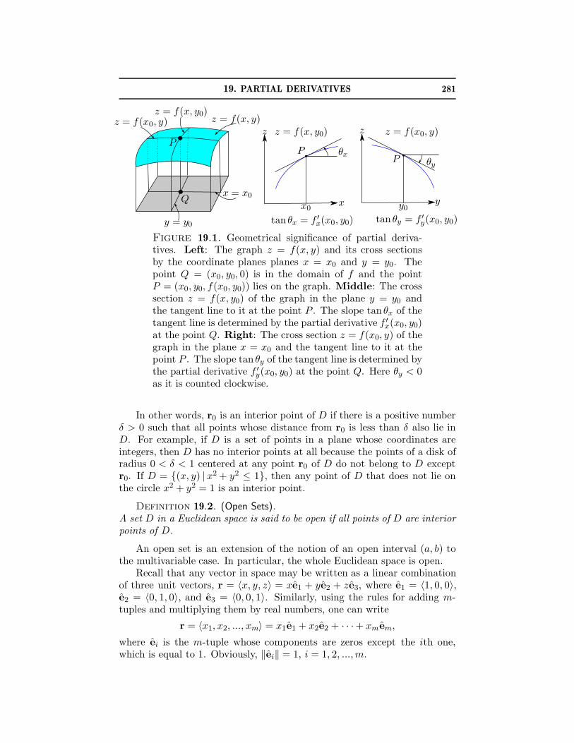
19. PARTIAL DERIVATIVES 281
P
Q
z = f(x0, y)z = f(x, y0)
z = f(x, y)
y = y0
x = x0
z
x
P
x0
θx
z = f(x, y0)
tan θx = f ′x(x0, y0)
z
yy0
P
tan θy = f ′y(x0, y0)
θy
z = f(x0, y)
Figure 19.1. Geometrical significance of partial deriva-tives. Left: The graph z = f(x, y) and its cross sectionsby the coordinate planes planes x = x0 and y = y0. Thepoint Q = (x0, y0, 0) is in the domain of f and the pointP = (x0, y0, f(x0, y0)) lies on the graph. Middle: The crosssection z = f(x, y0) of the graph in the plane y = y0 andthe tangent line to it at the point P . The slope tan θx of thetangent line is determined by the partial derivative f ′
x(x0, y0)at the point Q. Right: The cross section z = f(x0, y) of thegraph in the plane x = x0 and the tangent line to it at thepoint P . The slope tan θy of the tangent line is determined bythe partial derivative f ′
y(x0, y0) at the point Q. Here θy < 0as it is counted clockwise.
In other words, r0 is an interior point of D if there is a positive numberδ > 0 such that all points whose distance from r0 is less than δ also lie inD. For example, if D is a set of points in a plane whose coordinates areintegers, then D has no interior points at all because the points of a disk ofradius 0 < δ < 1 centered at any point r0 of D do not belong to D exceptr0. If D = {(x, y) | x2 + y2 ≤ 1}, then any point of D that does not lie onthe circle x2 + y2 = 1 is an interior point.
Definition 19.2. (Open Sets).A set D in a Euclidean space is said to be open if all points of D are interiorpoints of D.
An open set is an extension of the notion of an open interval (a, b) tothe multivariable case. In particular, the whole Euclidean space is open.
Recall that any vector in space may be written as a linear combinationof three unit vectors, r = 〈x, y, z〉 = xe1 + ye2 + ze3, where e1 = 〈1, 0, 0〉,e2 = 〈0, 1, 0〉, and e3 = 〈0, 0, 1〉. Similarly, using the rules for adding m-tuples and multiplying them by real numbers, one can write
r = 〈x1, x2, ..., xm〉 = x1e1 + x2e2 + · · ·+ xmem,
where ei is the m-tuple whose components are zeros except the ith one,which is equal to 1. Obviously, ‖ei‖ = 1, i = 1, 2, ...,m.

282 3. DIFFERENTIATION OF MULTIVARIABLE FUNCTIONS
Definition 19.3. (Partial Derivatives at a Point).Let f be a function of several variables (x1, x2, ..., xm). Let D be the domainof f and let r0 be an interior point of D. If the limit
f ′xi
(r0) = limh→0
f(r0 + hei) − f(r0)
h
exists, then it is called the partial derivative of f with respect to xi at r0.
The reason the point r0 needs to be an interior point is simple. Bythe definition of the one-variable limit, h can be negative or positive. Sothe points r0 + hei, i = 1, 2, ..., m, must be in the domain of the functionbecause otherwise f(r0 +hei) is not even defined. This is guaranteed if r0 isan interior point because all points r in a neighborhood Nδ(r0) of sufficientlysmall radius δ are in D; the points r0 + hei lie in D if |h| < δ.
Remark. It is also common to omit “prime” in the notations for partialderivatives. For example, the partial derivatives of f(x, y) at a point (x0, y0)are denoted as fx(x0, y0) and fy(x0, y0). In what follows, the notation in-troduced in Definition 19.3 will be used.
Let r0 = 〈a1, a2, ..., am〉, where ai are fixed numbers. Consider the func-tion F (xi) of one variable xi (i is fixed), which is obtained from f(r) bysetting all the variables to a number xj = aj except the ith one (i.e., xj = aj
for all j 6= i). By the definition of the ordinary derivative, the partial deriv-ative f ′
xi(r0) exists if and only if the derivative F ′(ai) exists because
(19.1) f ′xi
(r0) = limh→0
F (ai + h)− F (ai)
h=
dF (xi)
dxi
∣
∣
∣
xi=ai
just like in the case of two variables discussed at the beginning of this section.This rule is practical for calculating partial derivatives as it reduces theproblem to computing ordinary derivatives.
Example 19.1. Find the partial derivatives of f(x, y, z) = x3 − y2z atthe point (1, 2, 3).
Solution: By the rule (19.1),
f ′x(1, 2, 3) =
d
dxf(x, 2, 3)
∣
∣
∣
x=1=
d
dx(x3 − 12)
∣
∣
∣
x=1= 3,
f ′y(1, 2, 3) =
d
dyf(1, y, 3)
∣
∣
∣
y=2=
d
dy(1− 3y2)
∣
∣
∣
y=2= −12,
f ′z(1, 2, 3) =
d
dzf(1, 2, z)
∣
∣
∣
z=3=
d
dz(1 − 4z)
∣
∣
∣
z=3= −4.
�
Geometrical Significance of Partial Derivatives. From the rule (19.1), itfollows that the partial derivative f ′
xi(r0) defines the rate of change of the
function f when only the variable xi changes while the other variables are
19. PARTIAL DERIVATIVES 283
kept fixed. If, for instance, the function f in Example 19.1 defines thetemperature in degrees Celsius as a function of position whose coordinatesare given in meters, then, at the point (1, 2, 3), the temperature increasesat the rate 3 degrees Celsius per meter in the direction of the x axis, and itdecreases at the rates −12 and −4 degrees Celsius per meter in the directionof the y and z axes, respectively.
19.2. Partial Derivatives as Functions. Suppose that the partial derivativesof f exist at all points of a set D. Then each partial derivative can beviewed as a function of several variables on D. These functions are denotedas f ′
xi(r), where r ∈ D. They can be found by the same rule (19.1) if,
when differentiating with respect to xi, all other variables are not set to anyspecific values but rather viewed as independent of xi (i.e., dxj/dxi = 0 forall j 6= i). This agreement is reflected by the notation
f ′xi
(x1, x2, ..., xm) =∂
∂xif(x1, x2, ..., xm);
that is, the symbol ∂/∂xi means differentiation with respect to xi whileregarding all other variables as numerical parameters independent of xi.
Example 19.2. Find f ′x(x, y) and f ′
y(x, y) if f(x, y) = x sin(xy).
Solution: Assuming first that y is a numerical parameter independent ofx, one obtains
f ′x(x, y) =
∂
∂xf(x, y) =
( ∂
∂xx)
sin(xy) + x∂
∂xsin(xy)
= sin(xy) + xy cos(xy)
by the product rule for the derivative. If now the variable x is viewed as anumerical parameter independent of y, one obtains
f ′y(x, y) =
∂
∂yf(x, y) = x
∂
∂ysin(xy) = x2 cos(xy).
�
19.3. Basic Rules of Differentiation. Since a partial derivative is just anordinary derivative with one additional agreement that all other variablesare viewed as numerical parameters, the basic rules of differentiation applyto partial derivatives. Let f and g be functions of several variables and letc be a number. Then
∂
∂xi(cf) = c
∂f
∂xi,
∂
∂xi(f + g) =
∂f
∂xi+
∂g
∂xi,
∂
∂xi(fg) =
∂f
∂xig + f
∂g
∂xi,
∂
∂xi
(f
g
)
=
∂f∂xi
g − f ∂g∂xi
g2.
Let h(u) be a differentiable function of one variable and let g(r) be a functionof several variables whose range lies in the domain of h. Then one can define

284 3. DIFFERENTIATION OF MULTIVARIABLE FUNCTIONS
the composition f(r) = h(g(r)). Assuming that the partial derivatives of gexist, the chain rule holds
(19.2)∂f
∂xi= h′(g)
∂g
∂xi.
Example 19.3. Find the partial derivatives of the function f(r) =‖r‖−1, where r = 〈x1, x2, ..., xm〉.
Solution: Put h(g) = g−1/2 and g = g(r) = x21 + x2
2 + · · · + x2m = ‖r‖2.
Then f(r) = h(g(r)). Since h′(g) = (−1/2)g−3/2 and ∂g/∂xi = 2xi, thechain rule gives
∂
∂xi
1
‖r‖ =(
− 1
2g3/2
)
(2xi) = − xi
‖r‖3, i = 1, 2, ...,m .
�
19.4. Exercises.1-7. Find the specified partial derivatives of each of the following functions:
1. f(x, y) = (x − y)/(x + y), f ′x(1, 2), f ′
y(1, 2) ;
2. f(x, y, z) = (xy + z)/(z + y), f ′x(1, 2, 3), f ′
y(1, 2, 3), f ′z(1, 2, 3) ;
3. f(r) = (x1 + 2x2 + · · ·+ mxm)/(1 + ‖r‖2), f ′xi
(0), i = 1, 2, ...,m ;4. f(x, y, z) = x sin(yz), f ′
x(1, 2, π/2), f ′y(1, 2, π/2), f ′
z(1, 2, π/2);
5. f(x, y) = x + (y − 1) sin−1(√
x/y), f ′x(1, 1), f ′
y(1, 1) ;
6. f(x, y) = (x3 + y3)1/3, f ′x(0, 0), f ′
y(0, 0) ;
7. f(x, y) =√
|xy|, f ′x(0, 0), f ′
y(0, 0) .
8-23. Find the partial derivatives of each of the following functions:
8. f(x, y) = (x + y2)n ;9. f(x, y) = xy ;
10. f(x, y) = xe(x+2y)2 ;11. f(x, y) = sin(xy) cos(x2 + y2) ;12. f(x, y, z) = ln(x + y2 + z3) ;13. f(x, y, z) = xy2 cos(z2x) ;14. f(r) = (a1x1 + a2x2 + · · ·+ amxm)n = (a · r)n ;15. f(x, y) = tan−1(y/x) ;
16. f(x, y) = sin−1(x/√
x2 + y2) ;17. f(x, y, z) = xyz
;
18. f(x, y, z) = xy/z ;19. f(x, y) = tan(x2/y) ;20. f(x, y, z) = sin(x sin(y sin z)) ;21. f(x, y) = (x + y2)/(x2 + y) ;22. f(x, y, z) = a · (b× r), where a and b are constant vectors ;23. f(x, y, z) = ‖a× r‖, where a is a constant vector .

19. PARTIAL DERIVATIVES 285
24-28. For each of the following functions, determine whether the functionf increases or decreases at a specified point P0 when one variable increases,while the others are fixed:
24. f(x, y) = xy/(x + y), P0 = (1, 2) ;
25. f(x, y) = (x2 − 2y2)1/3, P0 = (1, 1) ;26. f(x, y) = x2 sin(xy), P0 = (−1, π) ;27. f(x, y, z) = zx/(x + y2), P0 = (1, 1, 1) ;
28. f(x, y, z) = (x + yz)/√
x + 2y + z2, P0 = (1, 2, 2).
286 3. DIFFERENTIATION OF MULTIVARIABLE FUNCTIONS
20. Higher-Order Partial Derivatives
Since partial derivatives of a function are also functions of several vari-ables, they can be differentiated with respect to any variable. For example,for a function of two variables, all possible second partial derivatives are
∂f
∂x7−→ ∂
∂x
∂f
∂x=
∂2f
∂x2,
∂
∂y
∂f
∂x=
∂2f
∂y ∂x,
∂f
∂y7−→ ∂
∂x
∂f
∂y=
∂2f
∂x ∂y,
∂
∂y
∂f
∂y=
∂2f
∂y2.
Throughout the text, brief notations for higher-order partial derivatives willalso be used. For example,
∂2f
∂x2= (f ′
x)′x = f ′′xx ,
∂2f
∂x ∂y= (f ′
y)′x = f ′′
yx
and similarly for f ′′yy and f ′′
xy. Partial derivatives of the third order aredefined as partial derivatives of second partial derivatives, and so on.
Example 20.1. For the function f(x, y) = x4−x2y +y2, find all secondand third partial derivatives.
Solution: The first partial derivatives are
f ′x = 4x3 − 2xy , f ′
y = −x2 + 2y .
Then the second partial derivatives are
f ′′xx = (4x3 − 2xy)′x = 12x2 − 2y , f ′′
yy = (−x2 + 2y)′y = 2,
f ′′xy = (4x3 − 2xy)′y = −2x , f ′′
yx = (−x2 + 2y)′x = −2x .
The third partial derivatives are found similarly:
f′′′
xxx = (12x2 − 2y)′x = 24x , f′′′
yyy = (2)′y = 0,
f′′′
xxy = (12x2 − 2y)′y = −2 , f′′′
xyx = f′′′
yxx = (−2x)′x = −2,
f′′′
yyx = (2)′x = 0 , f′′′
yxy = f′′′
xyy = (−2x)′y = 0.
�
In contrast to the one-variable case, there are higher-order partial deriva-tives of a new type that are obtained by differentiating with respect to dif-ferent variables in different orders, like f ′′
xy and f ′′yx. In the above example,
it has been found that
f ′′xy = f ′′
yx,
f′′′
xxy = f′′′
xyx = f′′′
yxx,
f′′′
xyy = f′′′
yyx = f′′′
yxy;
that is, the result is independent of the order in which the partial derivativeshave been taken. Is this a peculiarity of the function considered or a general
20. HIGHER-ORDER PARTIAL DERIVATIVES 287
property of higher-order partial derivatives? The following theorem answersthis question.
Theorem 20.1. (Clairaut’s Theorem).Let f be a function of several variables (x1, x2, ..., xm) that is defined on anopen ball D in a Euclidean space. If the second partial derivatives f ′′
xixjand
f ′′xjxi
, where j 6= i, are continuous functions on D, then f ′′xixj
= f ′′xjxi
at anypoint of D.
A consequence of Clairaut’s theorem can be proved. It asserts that:
The result of partial differentiation does not depend on the order in whichthe partial derivatives have been taken if all higher-order partial derivativesin question are continuous.
It is not always necessary to calculate higher-order partial derivatives inall possible orders to verify the hypothesis of Clairaut’s theorem (i.e., thecontinuity of the partial derivatives). Partial derivatives of polynomials arepolynomials and hence continuous. By the quotient rule for partial deriva-tives, rational functions have continuous partial derivatives (where the de-nominator does not vanish). Derivatives of basic elementary functions likethe sine and cosine and exponential functions are continuous. So composi-tions of these functions with multivariable polynomials or rational functionshave continuous partial derivatives of any order. In other words, the conti-nuity of higher-order partial derivatives can often be established by different,simpler means.
Example 20.2. Find the third derivatives f′′′
xyz, f′′′
yzx, f′′′
zxy, and so on,
for all permutations of x, y, and z, if f(x, y, z) = sin(x2 + yz).
Solution: The sine and cosine functions are continuously differentiable asmany times as desired. The argument of the sine function is a multivari-able polynomial. By the chain rule, (sin g)′x = g′x cos g and similarly for theother partial derivatives. Therefore partial derivatives of any order mustbe products of polynomials and the sine and cosine functions whose argu-ment is a polynomial. Therefore, they are continuous in the entire space.The hypothesis of Clairaut’s theorem is satisfied, and hence all the partialderivatives in question coincide and are equal to
f′′′
xyz = (f ′x)′′yz = (2x cos(x2 + yz))′′yz = (−2xz sin(x2 + yz))′z
= −2x sin(x2 + yz) − 2xyz cos(x2 + yz) .
�
20.1. Reconstruction of a Function from Its Partial Derivatives. One ofthe standard problems in calculus is finding a function f(x) if its derivative
288 3. DIFFERENTIATION OF MULTIVARIABLE FUNCTIONS
f ′(x) = G(x) is known. A sufficient condition for the existence of a solutionis the continuity of G(x). In this case,
f ′(x) = G(x) =⇒ f(x) =
∫
G(x) dx .
A similar problem can be posed for a function of several variables. Giventhe first partial derivatives
(20.1) f ′xi
(r) = Gi(r) , i = 1, 2, ...,m,
find f(r) if it exists. The existence of such f is a more subtle question inthe case of several variables. Suppose that the partial derivatives ∂Gi/∂xj
exist and are continuous functions in an open ball. Then taking the partialderivative ∂/∂xj of both sides of (20.1) and applying Clairaut’s theorem,one infers that
(20.2) f ′′xixj
= f ′′xjxi
=⇒ ∂Gi
∂xj=
∂Gj
∂xi.
Thus, the conditions (20.2) on the functions Gi must be fulfilled; other-wise, f satisfying (20.1) does not exist. The conditions (20.2) are calledintegrability conditions for the system of equations (20.1).
Example 20.3. Suppose that f ′x(x, y) = 2x + y and f ′
y(x, y) = 2y − x.Does such a function f exist?
Solution: The first partial derivatives of f ,
f ′x(x, y) = G1(x, y) = 2x + y , f ′
y(x, y) = G2(x, y) = 2y − x ,
are polynomials, and hence their partial derivatives are continuous in theentire plane. In order for f to exist, the integrability condition
∂G1
∂y=
∂G2
∂x
must hold in the entire plane. This is not so because
∂G1
∂y=
∂
∂y(2x + y) = 1 ,
∂G2
∂x=
∂
∂x(2y − x) = −1 ⇒ ∂G1
∂y6= ∂G2
∂x.
Thus, no such f exists. �
Suppose now that the integrability conditions (20.2) are satisfied. Howis a solution f to (20.1) to be found? Evidently, one has to calculate anantiderivative of the partial derivative. In the one-variable case, an anti-derivative on an interval is defined up to an additive constant. This is notso in the multivariable case. For example, consider the equation
f ′x(x, y) = 3x2y .
An antiderivative of f ′x is a function whose partial derivative with respect
to x is 3x2y. It is easy to verify that x3y satisfy this requirement. It isobtained by taking an antiderivative of 3x2y with respect to x while viewingy as a numerical parameter independent of x. Since f ′
x as a function of x is
20. HIGHER-ORDER PARTIAL DERIVATIVES 289
defined for all x (that is, on a single interval) at each fixed y, one can alwaysadd a constant to a particular antiderivative, x3y + c, and obtain anothersolution. The key point to observe is that the constant may be a functionof y only. Indeed, if c = g(y), then c′x = (g(y))′x = 0. Thus,
f ′x(x, y) = 3x2y ⇒ f(x, y) = x3y + g(y)
for some function g(y). If, in addition, the other partial derivative f ′y is
given, then an explicit form of g(y) can be found. Put, for example,
f ′x(x, y) = 3x2y
f ′y(x, y) = x3 + 2y
The integrability conditions are fulfilled:
(f ′x)′y = (3x2y)′y = 3x2
(f ′y)
′x = (x3 + 2y)′x = 3x2 ⇒ f ′′
xy(x, y) = f ′′yx(x, y)
So a function with the said partial derivatives does exist. The obtainedgeneral solution to the first equation is substituted into the second equationto find an equation for the unknown function g(y):
f(x, y) = x3y + g(y)f ′y(x, y) = x3 + 2y
⇒ (x3y + g(y))′y = x3 + 2y ⇒ g′(y) = 2y
Therefore g(y) = y2 + c and f(x, y) = x3y + y2 + c.
Remark. In the above example, note the cancellation of the x3 term in theequation for g(y). This is a direct consequence of the fulfilled integrabilitycondition. Had one tried to apply the same procedure to a similar problemwithout checking the integrability conditions, one could have found that, ingeneral, no such g(y) exists. In Example 20.3, the equation f ′
x = 2x+ y hasa general solution f(x, y) = x2 + yx + g(y). Its substitution into the secondequation f ′
y = 2y − x yields
f(x, y) = x2 + yx + g(y)f ′y(x, y) = 2y − x
⇒ x + g′(y) = 2y − x ⇒ g′(y) = 2y − 2x .
The derivative of g(y) cannot depend on x and hence no such g(y) exists.
Example 20.4. Find f(x, y, z) if f ′x = yz + 2x, f ′
y = xz + 3y2, and
f ′z = xy + 4z3 or show that it does not exist.
Solution: The integrability conditions have to be verified first:
(G1)′y = (G2)
′x ,
(G1)′z = (G3)
′x ,
(G2)′z = (G3)
′y ,
G1 = yz + 2x
G2 = xz + 3y2
G3 = xy + 4z3
⇒(yz + 2x)′y = (xz + 3y2)′x(yz + 2x)′z = (xy + 4z3)′x
(xz + 3y2)′z = (xy + 4z3)′y
The calculation of the partial derivatives in the last three equations yields,respectively, z = z, y = y, and x = x so that the integrability conditions are
290 3. DIFFERENTIATION OF MULTIVARIABLE FUNCTIONS
satisfied. Therefore f exists. Taking the antiderivative with respect to x inthe first equation, one finds
f ′x = yz + 2x ⇒ f(x, y, z) = xyz + x2 + g(y, z) ,
for some g(y, z). The substitution of f into the second equations yields
f ′y = xz + 3y2 ⇒ xz + g′y(y, z) = xz + 3y2
⇒ g′y(y, z) = 3y2 ⇒ g(y, z) = y3 + h(z)
⇒ f(x, y, z) = xyz + x2 + y3 + h(z),
for some h(z). The substitution of f into the third equation yields
f ′z = xy + 4z3 ⇒ xy + h′(z) = xy + 4z3
⇒ h′(z) = 4z3
⇒ h(z) = z4 + c
⇒ f(x, y, z) = xyz + x2 + y3 + z4 + c,
where c is a constant. �
The procedure of reconstructing f from its first partial derivatives aswell as the integrability conditions (20.2) will be important when discussingconservative vector fields and the potential of a conservative vector field.
20.2. Partial Differential Equations. The relation between a function ofseveral variables and its partial derivatives (of any order) is called a partialdifferential equation. Partial differential equations are a key tool to studyvarious phenomena in nature. Many fundamental laws of nature can bestated in the form of partial differential equations.
Diffusion Equation. Let n(r, t), where r = 〈x, y, z〉 is the position vector inspace and t is time, be a concentration of a substance, say, in air or water oreven in a solid. Even if there is no macroscopic motion in the medium, theconcentration changes with time due to thermal motion of the molecules.This process is known as diffusion. In some simple situations, the rate atwhich the concentration changes with time at a point is
n′t = k(n′′
xx + n′′yy + n′′
zz),
where the parameter k is a diffusion constant. So the concentration asa function of the spatial position and time must satisfy the above partialdifferential equation.
Wave Equation. Sound in air is propagating disturbances of the air density.If u(r, t) is the deviation of the air density from its constant (nondisturbed)value u0 at the spatial point r = 〈x, y, z〉 and at time t, then it can be shownthat disturbances of the air density small compared to u0 satisfy the waveequation:
u′′tt = c2(u′′
xx + u′′yy + u′′
zz),
20. HIGHER-ORDER PARTIAL DERIVATIVES 291
where c is the speed of sound in the air (its values depends on u0 and theair pressure). Light is an electromagnetic wave. Its propagation is alsodescribed by the wave equation, where c is the speed of light in vacuum (orin a medium, if light goes through a medium) and u is the amplitude ofelectric or magnetic fields.
Laplace and Poisson Equations. The equation
u′′xx + u′′
yy + u′′zz = f,
where f is a given non-zero function of position r = 〈x, y, z〉 in space, iscalled the Poisson equation. In the special case when f = 0, this equation isknown as the Laplace equation. The Poisson and Laplace equations are usedto determine static electromagnetic fields created by static electric chargesand currents.
Example 20.5. Let h(q) be a twice-differentiable function of a variableq. Show that u(r, t) = h(ct− n · r) is a solution of the wave equation for anyfixed unit vector n.
Solution: Let n = (n1, n2, n3), where n21 + n2
2 + n23 = 1 as n is the unit
vector. Putq = ct − n · r = ct − n1x − n2y − n3z .
By the chain rule (19.2), u′t = q′th
′(q) and similarly for the other partialderivatives. Therefore
u′t = ch′(q)
u′x = −n1h
′(q)
u′y = −n2h
′(q)
u′z = −n3h
′(q)
⇒
u′′tt = c2h′′(q)
u′′xx = n2
1h′′(q)
u′′yy = n2
2h′′(q)
u′′zz = n2
3h′′(q)
Then
c2(u′′xx + u′′
yy + u′′zz) = c2(n2
1 + n22 + n2
3)h′′(q) = c2h′′(q) = u′′
tt
which means that the wave equation is satisfied for any h. �
Consider the level sets of the solution of the wave equation discussedin this example. They correspond to a fixed value of q = q0. So, for eachmoment of time t, the disturbance of the air density u(r, t) has a constantvalue h(q0) in the plane
n · r = ct − q0 = d(t) .
All planes with different values of the parameter d are parallel as they havethe same normal vector n. Since here d(t) is a function of time, the plane onwhich the air density has a fixed value moves along the vector n at the rated′(t) = c. Thus, a disturbance of the air density propagates with speed c.This is the reason that the constant c in the wave equation is called the speedof sound. Evidently, the same line of arguments applies to electromagneticwaves; that is, they move through space at the speed of light. The speed of
292 3. DIFFERENTIATION OF MULTIVARIABLE FUNCTIONS
sound in the air is about 342 meters per second, or about 768 mph. Thespeed of light is 3 · 108 meters per second, or 186 miles per second. If alightning strike occurs a mile away during a thunderstorm, it can be seenalmost instantaneously, while the thunder will be heard in about 5 secondslater. Conversely, if one sees a lightning and starts counting seconds untilthe thunder is heard, then one could determine the distance to the lightning.The sound travels 1 mile in about 4.7 seconds.
20.3. Study Problems.
Problem 20.1. Consider the function
f(x, y) =x3y − xy3
x2 + y2if (x, y) 6= (0, 0) and f(0, 0) = 0.
Find f ′x(x, y) and f ′
y(x, y) for (x, y) 6= (0, 0). Use the rule (19.1) to find
f ′x(0, 0) and f ′
y(0, 0) and, thereby, to establish that f ′x and f ′
y exist every-
where. Use the rule (19.1) again to show that f ′′xy(0, 0) = −1 and f ′′
yx(0, 0) =
1, that is, f ′′xy(0, 0) 6= f ′′
yx(0, 0). Does this result contradict Clairaut’s theo-rem?
Solution: Using the quotient rule for differentiation, one finds
f ′x(x, y) =
x4y + 4x2y3 − y5
(x2 + y2)2, f ′
y(x, y) =x5 − 4x3y2 − xy4
(x2 + y2)2
if (x, y) 6= (0, 0). Note that, owing to the symmetry f(x, y) = −f(y, x), thepartial derivative f ′
y is obtained from f ′x by changing the sign of the latter
and swapping x and y. The partial derivatives at (0, 0) are found by therule (19.1):
f ′x(0, 0) =
d
dxf(x, 0)
∣
∣
∣
x=0= 0 , f ′
y(0, 0) =d
dyf(0, y)
∣
∣
∣
y=0= 0.
The first-order partial derivatives are continuous functions for all (x, y) 6=(0, 0). Put
√
x2 + y2 = R. Then using |x| ≤ R and |y| ≤ R,
|f ′x(x, y)| = |x4y + 4x2y3 − y5|
R4≤ R5 + 4R5 + R5
R4= 6R → 0
as R → 0+. Therefore by the squeeze principle, f ′x(x, y) → 0 = f ′
x(0, 0)as (x, y) → (0, 0). So, f ′
x(x, y) is continuous everywhere. The continuity off ′y(x, y) at the origin is established similarly.
20. HIGHER-ORDER PARTIAL DERIVATIVES 293
Next, one has
f ′′xy(0, 0) =
d
dyf ′x(0, y)
∣
∣
∣
y=0= lim
h→0
f ′x(0, h)− f ′
x(0, 0)
h
= limh→0
−h − 0
h= −1,
f ′′yx(0, 0) =
d
dxf ′y(x, 0)
∣
∣
∣
x=0= lim
h→0
f ′y(h, 0)− f ′
y(0, 0)
h
= limh→0
h − 0
h= 1.
The result does not contradict Clairaut’s theorem because f ′′xy(x, y) and
f ′′yx(x, y) are not continuous at (0, 0). By using the quotient rule to differen-
tiate f ′x(x, y) with respect to y, an explicit form of f ′′
xy(x, y) can be obtained
for (x, y) 6= (0, 0). By taking the limit of f ′′xy(x, y) as (x, y) → (0, 0) along
the straight line (x, y) = (t, at), t → 0+, one infers that the limit dependson the slope a and hence the two-dimensional limit does not exist, that is,lim(x,y)→(0,0) f ′′
xy(x, y) 6= f ′′xy(0, 0) = −1 and f ′′
xy is not continuous at (0, 0).The technical details are left to the reader. �
Problem 20.2. Find the value of a constant a for which the function
u(r, t) = t−3/2e−ar2/t , r = ‖r‖,
satisfies the diffusion equation for all t > 0.
Solution: Note that u depends on the combination r2 = x2 + y2 + z2. Tofind the partial derivatives of u, it is convenient to use the chain rule:
∂u
∂x=
∂u
∂r2
∂r2
∂x= 2x
∂u
∂r2= −2ax
tu,
u′′xx =
∂
∂x
(∂u
∂x
)
= −2a
tu − 2ax
t
∂u
∂x=
(
−2k
t+
4a2x2
t2
)
u.
To obtain u′′yy and u′′
zz , note that r2 is symmetric with respect to permu-tations of x, y, and z. Therefore, u′′
yy and u′′zz are obtained from u′′
xx byreplacing, in the latter, x by y and x by z, respectively. Hence, the rightside of the diffusion equation reads
k(u′′xx + u′′
yy + u′′zz) =
(
− 6ka
t+
4ka2r2
t2
)
u.
Using the product rule to calculate the partial derivative with respect totime, one finds for the left side of the diffusion equation
u′t = −3
2t−5/2e−ar2/t + t−3/2e−ar2/tar2
t2=
(
− 3
2t+
ar2
t2
)
u.
294 3. DIFFERENTIATION OF MULTIVARIABLE FUNCTIONS
Since both sides must be equal for all values of t > 0 and r2, the comparisonof the last two expressions yields two conditions:
u′t = k(u′′
xx + u′′yy + u′′
zz) ⇒{
6ka = 32
a = 4ka2 ⇒ a =1
4k,
where the equality means matching the coefficients at 1/t and the secondone is needed to match the coefficients at r2/t2. The only common solutionof these equations is a = 1/(4k). �
20.4. Exercises.1–6. Find all second partial derivatives of each of the following functionsand verify Clairaut’s theorem:
1. f(x, y) = tan−1(xy) ;2. f(x, y, z) = x sin(zy2) ;3. f(x, y, z) = x3 + zy + z2 ;4. f(x, y, z) = (x + y)/(x + 2z) ;
5. f(x, y) = cos−1(√
x/y) ;6. f(x, y) = xy ;7. f(x1, x2, ..., xm) = (a · r)(b · r) ,where r = 〈x1, x2, ..., xm〉 and a
and b are constant vectors.
8–12. Show without explicit calculations of higher-order partial derivativeswhy the hypotheses of Clairaut’s theorem are satisfied for the followingfunctions:
8. f(x, y, z) = sin(x2 + y − z) cos(xy) ;9. f(x, y) = sin(x + y2)/(x2 + y2), x2 + y2 6= 0 ;
10. f(x, y, z) = ex2yz(y2 + zx4) ;11. f(x, y) = ln(1 + x2 + y4)/(x2 − y2), x2 6= y2 ;12. f(x, y, z) = (x + yz2 − xz5)/(1 + x2y2z4) .
13-20. Find the indicated partial derivatives of each of the following func-tions:
13. f(x, y) = xn + xy + ym, f ′′′xxy, f ′′′
xyx, f ′′′yyx, f ′′′
xyy ; here n and m arepositive integers ;
14. f(x, y, z) = x cos(yx) + z3, f ′′′xyz, f ′′′
xxz, f ′′′yyz ;
15. f(x, y, z) = sin(xy)ez, ∂f5/∂z5, f(4)xyzz , f
(4)zyxz , f
(4)zxzy ;
16. f(x, y, z, t) = sin(x + 2y + 3z − 4t), f(4)abcd where abcd denotes all
permutations of xyzt ;
17. f(x, y) = exy(y2 +x), f(4)abcd where abcd denotes all permutations
of xxxy ;
18. f(x, y, z) = tan−1(
x+y+z−xyz1−xy−xz−yz
)
, f(3)abc where abc denotes all per-
mutations of xyz ;
19. f(x, y, z, t) = ln(
(x− y)2 + (z − t)2)−1/2
, f(4)abcd where abcd are
all permutations of xyzt ;
20. HIGHER-ORDER PARTIAL DERIVATIVES 295
20. f(x, y) = ex sin(y), ∂n+mf∂nx∂my (0, 0), where n and m are positive
integers.
21-25. Given partial derivatives, find the function or show that it does notexist:
21. f ′x = 3x2y, f ′
y = x3 + 3y2 ;
22. f ′x = yz + 3x2, f ′
y = xz + 4y, f ′z = xy + 1 ;
23. f ′xk
= kxk, k = 1, 2, ...,m ;
24. f ′x = xy + z, f ′
y = x2/2, f ′z = x + y ;
25. f ′x = sin(xy) + xy cos(xy), f ′
y = x2 cos(xy) + 1 .
26-32. Verify that a given function is a solution of the indicated differentialequation:
26. f(t, x) = A sin(ct − x) + B cos(ct + x), c−2f ′′tt − f ′′
xx = 0 if A, B,and c are constants ;
27. f(x, y, t) = g(ct− ax− by)+ h(ct + ax + by), f ′′tt = c2(f ′′
xx + f ′′yy)
if a, b, and c are constants such that a2 + b2 = 1, and g and h aretwice differentiable functions ;
28. f(x, y) = ln(x2 + y2), f ′′xx + f ′′
yy = 0 ;
29. f(x, y) = ln(ex + ey), f ′x + f ′
y = 1 and f ′′xxf ′′
yy − (f ′′xy)
2 = 0 ;30. f(r) = exp(a · r), where a · a = 1 and r ∈ R
m,f ′′x1x1
+ f ′′x2x2
+ · · ·+ f ′′xmxm
= f ;
31. f(r) = ‖r‖2−m, where r ∈ Rm , f ′′
x1x1+ f ′′
x2x2+ · · ·+ f ′′
xmxm= 0
for ‖r‖ 6= 0 ;32. f(x, y, z) = sin(k‖r‖)/‖r‖, f ′′
xx + f ′′yy + f ′′
zz + k2f = 0 (Helmholtzequation), where k is a constant .
33. Find a relation between constants a, b and c such that the functionu(x, y, t) = sin(ax + by + ct) satisfies the wave equation u′′
tt − u′′xx − u′′
yy = 0.Give a geometrical description of such a relation, e.g., by setting values of con a vertical axis, and the values of a and b on two horizontal axes.
34. Let f(x, y, z) = u(t) where t = xyz. Show that f(3)xyz = F (t) and find
F (t) in terms of u(t).35-36. Find (f ′
x)2+(f ′
y)2+(f ′z)
2 and f ′′xx+f ′′
yy +f ′′zz for each of the following
functions:
35. f = x3 + y3 + z3 − 3xyz ;36. f = (x2 + y2 + z2)−1/2 .
37-38. Let the action of K on a function f be defined by Kf = xf ′x + yf ′
y.
Find Kf , K2f = K(Kf), and K3f = K(K2f) if
37. f = x/(x2 + y2) ;
38. f = ln√
x2 + y2 .
39. Let f(x, y) = xy2/(x2 + y2) if (x, y) 6= (0, 0) and f(0, 0) = 0. Dof ′′xy(0, 0) and f ′′
yx(0, 0) exist?

296 3. DIFFERENTIATION OF MULTIVARIABLE FUNCTIONS
40–43. If f = f(x, y) and g = g(x, y, z), find the most general solution toeach of the following equations:
40. f ′′xx = 0 ;
41. f ′′xy = 0 ;
42. ∂nf/∂yn = 0 ;43. g′′′xyz = 0 .
44–46. Find f(x, y) that satisfies the given conditions:
44. f ′y = x2 + 2y, f(x, x2) = 1 ;
45. f ′′yy = 4, f(x, 0) = 2, f ′
y(x, 0) = x ;
46. f ′′xy = x + y, f(x, 0) = x, f(0, y) = y2 .
21. DIFFERENTIABILITY OF MULTIVARIABLE FUNCTIONS 297
21. Differentiability of Multivariable Functions
A differentiable one-variable function f(x) can be approximated nearx = x0 by its linearization
L(x) = f(x0) + f ′(x0)(x − x0)
or the tangent line. Put x = x0+∆x. Then by the definition of the derivativef ′(x0),
lim∆x→0
f(x) − L(x)
∆x= lim
∆x→0
f(x0 + ∆x) − f(x0)
∆x− f ′(x0)
= f ′(x0) − f ′(x0) = 0
This relation implies that the error of the linear approximation goes to 0faster than the deviation ∆x = x − x0 of x from x0, that is,
(21.1) f(x) = L(x) + ε(∆x) ∆x, where ε(∆x) → 0 as ∆x → 0 .
For example, if f(x) = x2, then its linearization at x = 1 is
L(x) = 1 + 2(x − 1) ,
It follows that near x = 1
f(1 + ∆x)− L(1 + ∆x) = (∆x)2 ⇒ ε(∆x) = ∆x .
Conversely, consider a line through the point (x0, f(x0)) and demandthat the condition (21.1) holds. If n is the slope of the line, then
L(x) = f(x0) + n(x − x0) = f(x0) + n∆x
and (21.1) implies that
lim∆x→0
f(x)− L(x)
∆x= lim
∆x→0
f(x0 + ∆x) − f(x0)
∆x− n = 0
By the definition of the derivative f ′(x0), the existence of this limit impliesthe existence of f ′(x0) and the equality n = f ′(x0). Thus, among all linearapproximations of f near x0, only the line with the slope n = f ′(x0) is agood approximation in the sense that the error of the approximation de-creases faster than ∆x with decreasing ∆x. The above analysis shows that:
A function f(x) is differentiable at x = x0 if and only if it has a goodlinear approximation at x = x0, that is, there is a linear function L(x) suchthat
limx→x0
f(x) − L(x)
x − x0= 0 .
298 3. DIFFERENTIATION OF MULTIVARIABLE FUNCTIONS
21.1. Tangent plane to a surface. Let us try to extend the concept of agood linear approximation at a point to functions of two variables. Considerthe graph z = f(x, y) of a continuous two-variable function. Then thegraph is a surface. Let a point P0 = (x0, y0, z0) be on this surface, that is,z0 = f(x0, y0). A linear approximation to f at (x0, y0), or the most generallinear function L(x, y) with the property L(x0, y0) = f(x0, y0) = z0, has theform
L(x, y) = z0 + n1(x − x0) + n2(y − y0) .
The graph
z = L(x, y) ⇒ n1(x − x0) + n2(y − y0) − (z − z0) = 0
is a plane through the point P0 on the graph z = f(x, y) with a normalvector n = 〈n1, n2,−1〉. How should the slopes in the x and y directions, n1
and n2, be chosen in order for L(x, y) to be a good linear approximation?To answer this question, one might employ the following strategy. Con-
sider the curve of intersection of the graph with the coordinate plane x = x0.Its equation is z = f(x0, y). Then the vector function
r1(t) = 〈x0 , t , f(x0, t)〉traces out the curve of intersection. The curve goes through the point P0
and r1(y0) =−−→OP0. A tangent vector at the point P0 to this curve is
v1 = r′1(y0) = 〈0 , 1 , f ′y(x0, y0)〉
(see Fig. 21.1). Similarly, the graph z = f(x, y) intersects the coordinateplane y = y0 along the curve z = f(x, y0) whose parametric equations are
r2(t) = 〈t, y0, f(t, y0)〉 .
A tangent vector to this curve at the point P0 is
v2 = r′2(x0) = 〈1, 0, f ′x(x0, y0)〉 .
In order for these tangent vectors to exist, it has to be assumed that thefunction f has partial derivatives at (x0, y0). The lines through P0 andparallel to the vectors v1 and v2 are not parallel because v1 and v2 arenot parallel. By construction, these lines are good linear approximations totwo graphs, z = f(x0, y) and z = f(x, y0), in the surface z = f(x, y). It istherefore natural to assume the plane z = L(x, y) that provides a good linearapproximation to the surface z = f(x, y) at a point P0 must contain the linesthat provide good linear approximations to two particular curves through P0
in the surface. Since these lines are not parallel, they define a unique planethat contains them.
Let us find this plane. A normal of this plane must be perpendicularto both vectors v1 and v2 and, by the geometrical properties of the crossproduct, may be taken as
n = v1 × v2 = 〈f ′x(x0, y0) , f ′
y(x0, y0) , −1〉 .
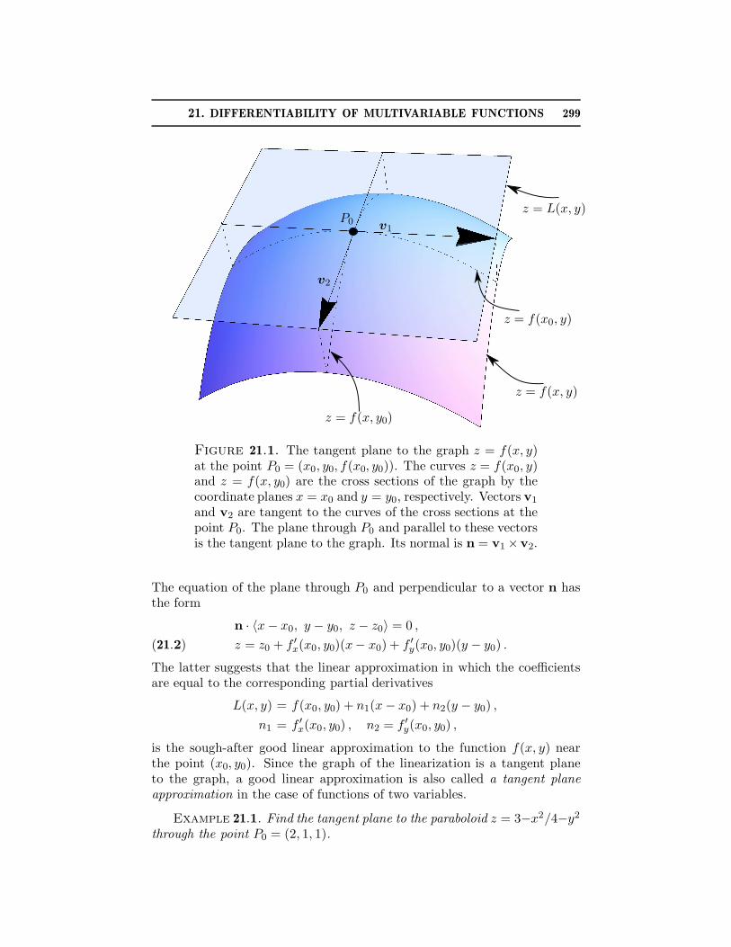
21. DIFFERENTIABILITY OF MULTIVARIABLE FUNCTIONS 299
z = L(x, y)
z = f(x, y)
z = f(x0, y)
P0v1
v2
z = f(x, y0)
Figure 21.1. The tangent plane to the graph z = f(x, y)at the point P0 = (x0, y0, f(x0, y0)). The curves z = f(x0, y)and z = f(x, y0) are the cross sections of the graph by thecoordinate planes x = x0 and y = y0, respectively. Vectors v1
and v2 are tangent to the curves of the cross sections at thepoint P0. The plane through P0 and parallel to these vectorsis the tangent plane to the graph. Its normal is n = v1 ×v2.
The equation of the plane through P0 and perpendicular to a vector n hasthe form
n · 〈x − x0, y − y0, z − z0〉 = 0 ,
z = z0 + f ′x(x0, y0)(x− x0) + f ′
y(x0, y0)(y − y0) .(21.2)
The latter suggests that the linear approximation in which the coefficientsare equal to the corresponding partial derivatives
L(x, y) = f(x0, y0) + n1(x − x0) + n2(y − y0) ,
n1 = f ′x(x0, y0) , n2 = f ′
y(x0, y0) ,
is the sough-after good linear approximation to the function f(x, y) nearthe point (x0, y0). Since the graph of the linearization is a tangent planeto the graph, a good linear approximation is also called a tangent planeapproximation in the case of functions of two variables.
Example 21.1. Find the tangent plane to the paraboloid z = 3−x2/4−y2
through the point P0 = (2, 1, 1).
300 3. DIFFERENTIATION OF MULTIVARIABLE FUNCTIONS
Solution: The paraboloid is the graph of the function
f(x, y) = 3 − x2
4− y2 , f(2, 1) = 1
The normal of the tangent plane is determined by the partial derivatives
f ′x(2, 1) =
d
dxf(x, 1)
∣
∣
∣
x=2=
(
2− x2
4
)′∣∣
∣
x=2= −x
2
∣
∣
∣
x=2= −1 ,
f ′y(2, 1) =
d
dyf(2, y)
∣
∣
∣
y=1= (2 − y2)′
∣
∣
∣
y=1= −2y
∣
∣
∣
y=1= −2 .
Therefore the equation for the tangent plane (21.2) reads
z = 1 − (x − 2)− 2(y − 1) or z = 5 − x − 2y .
�
21.2. Continuity and the Existence of Partial Derivatives. Let us examinehow good is the tangent plane approximation in Example 21.1. Followingthe analogy with the case of functions of one variable, one has to find howfast the error of the approximation decreases with decreasing the distancebetween (x, y) and (x0, y0) = (2, 1). Put x = 2 + ∆x and y = 1 + ∆y. Alinear approximation is given by the linear function L(x, y) = 5 − x − 2y =1 − ∆x − 2∆y (the graph z = L(x, y) is the tangent plane to the surfacez = f(x, y) at the point (2, 1)). Then
f(x, y)− L(x, y) = f(2 + ∆x, 1 + ∆y)− 1 + ∆x + 2∆y
= 3 − 1
4(2 + ∆x)2 − (1 + ∆y)2 − 1 + ∆x + 2∆y
= −1
4(∆x)2 − (∆y)2 .
The distance between (x, y) and (x0, y0) is R =√
(∆x)2 + (∆y)2. Therefore
|f(x, y)− L(x, y)|R
=(∆x)2/4 + (∆y)2
R≤ R2/4 + R2
R=
5
4R → 0
as R → 0. Thus, by the squeeze principle, the error of the approximationdecreases faster than R with decreasing R (it decreases as R2), and theconstructed linear approximation is a good one just like in the one-variablecase.
It seems that the mere existence of partial derivatives at a point is suffi-cient for the existence of a good linear approximation at that point. Unfor-tunately, this conclusion is wrong for functions of more than one variable!
Here is a simple counterexample. It is not difficult to see that the graphof the function in Example 21.1 is the paraboloid concave downward withvertex at (0, 0, 3). So the function attains its maximal value at (0, 0). Thepartial derivatives vanish at this point f ′
x(0, 0) = f ′y(0, 0) = 0. Hence, the
21. DIFFERENTIABILITY OF MULTIVARIABLE FUNCTIONS 301
tangent plane through the vertex of the paraboloid is the horizontal planez = 3. Let us change the function in the following way:
f(x, y) → g(x, y) =
{
0 , x > 0 , y > 03 − x2/4− y2 , otherwise
In other words, the function f has been changed by setting its values to zeroin the first quadrant, excluding the coordinate axes on which it retains itsold values
g(0, y) = f(0, y) = 3− y2 , g(x, 0) = f(x, 0) = 3 − x2/4
Therefore
g′y(0, 0) = f ′y(0, 0) = 0 , g′x(0, 0) = f ′
x(0, 0) = 0 .
It follows that the tangent plane to the graph z = g(x, y) at (0, 0) is also thehorizontal plane z = 3. But this horizontal plane is no good approximationat all! The difference g(x, y)− 3 remains equal to −3 for all x > 0, y > 0,no matter how close the point (x, y) to the origin (0, 0). It appears thatthe function g(x, y) is not even continuous at (0, 0), despite the existenceof its partial derivatives at (0, 0). The graph of f looks like a hill of theshape of a paraboloid, while the graph of g looks like the same hill withits south-east part (corresponding to the first quadrant) flatten, creating acliff, so that one can still walk on the edge of the cliff (corresponding to thepositive coordinate axes). At the top of the hill with such a cliff the slopesare still determined by (zero) slopes along the edges of the cliff, while theheight drops abruptly in the south-east direction. It is also interesting topoint out if the coordinate system relative to which the height of the hill isdetermined was rotated, say, by 45◦, one of the partial derivatives relativeto the new variables would not exist at the origin.
Example 21.2. Consider the function
f(x, y) =
{ xyx2+y2 if (x, y) 6= (0, 0)
0 if (x, y) = (0, 0).
Show that this function is not continuous at (0, 0), but that the partial deriva-tives f ′
x(0, 0) and f ′y(0, 0) exist.
Solution: In order to check the continuity, one has to calculate the limitlim(x,y)→(0,0) f(x, y). If it exists and equals f(0, 0) = 0, then the function iscontinuous at (0, 0). This limit does not exist. Along lines (x, y) = (t, at),the function has constant value
f(t, at) =at2
t2 + a2t2=
a
1 + a2, t 6= 0 .
Therefore the limit of f(x, y) as (x, y) → (0, 0) does not exist and the func-tion is not continuous at (0, 0). Note also that the non-existence of the limitmeans that the function is not even continuously extendable at (0, 0). Inother words, there is no value of f(0, 0) at which f would become continuous.
302 3. DIFFERENTIATION OF MULTIVARIABLE FUNCTIONS
The partial derivatives in question can be found by the rule 19.1:
f(x, 0) = 0 ⇒ f ′x(0, 0) =
d
dxf(x, 0)
∣
∣
∣
x=0= 0 ,
f(0, y) = 0 ⇒ f ′y(0, 0) =
d
dyf(0, y)
∣
∣
∣
y=0= 0 .
Thus, the partial derivatives exist at the origin, f ′x(0, 0) = fy(0, 0) = 0 but
f is not continuous at the origin. �
In the example considered, the plane defined by Eq. 21.2 at (x0, y0) =(0, 0) is z = 0. The deviation of the graph z = f(x, y) from the xy planeis finite along the lines (x, y) = (t, at), a 6= 0 no matter how close is t to 0.So, it does not even decrease with decreasing the distance from the origin!Thus, the tangent plane z = 0 defined by Eq. (21.2) no approximation atall to the graph of the function near the origin.
The above examples illustrate the following important relation betweenthe continuity and the existence of partial derivatives:
• The existence of partial derivatives at a point does not imply thatthe function is continuous at that point;
In full contrast to the one-variable case, this implies that the deviation ofthe plane defined by Eq. (21.2) from the graph z = f(x, y) may not be smallno matter how close is the point (x, y) to (x0, y0) even though f has partialderivatives at (x0, y0).
This is quite a departure from the one-variable case, where the existenceof the derivative at a point implied continuity at that point and was neces-sary and sufficient for the existence of a good linear approximation. This isthe reason that functions of several variables require a generalization of theconcept of differentiability. Differentiability of a function of several variablesat a point will be understood in the sense that the function has a good linearapproximation at that point.
21.3. Differentiability of multivariable functions. Consider a function oftwo variables f(x, y) and a point (x0, y0) in its domain. As already noted, themost general linear function L(x, y) with the property L(x0, y0) = f(x0, y0)has the form
L(x, y) = f(x0, y0) + n1(x − x0) + n2(y − y0)
where n1 and n2 are arbitrary numbers. It defines a linear approximationto f(x, y) near (x0, y0) in the sense that L(x0, y0) = f(x0, y0). This notionis extended to functions of any number of variables. Given a multivariablefunction f(r), a linear function
L(r) = f(r0) + n · (r− r0)
is said to be a linear approximation to f near r0 in the sense that L(r0) =f(r0). The dot product is defined in an m−dimensional Euclidean space if fis a function of m variables. The vector n is an arbitrary vector so that L(r)
21. DIFFERENTIABILITY OF MULTIVARIABLE FUNCTIONS 303
is the most general linear function satisfying the condition L(r0) = f(r0).Note that in the case of two variables x1 = x and x2 = y, n = 〈n1, n2〉 andr− r0 = 〈x− x0, y − y0〉 so that n · (r − r0) = n1(x− x0) + n2(y − y0).
Definition 21.1. (Differentiable Functions).The function f of several variables r = 〈x1, x2, ..., xm〉 on an open set D issaid to be differentiable at a point r0 of D if there exists a linear approxi-mation L(r) such that
(21.3) limr→r0
f(r)− L(r)
‖r− r0‖= 0.
If f is differentiable at all points of D, then f is said to be differentiable onD.
In what follows, functions differentiable on an open set will be calleddifferentiable. By this definition, the differentiability of a function is inde-pendent of a coordinate system chosen to label points of D (a linear functionremains linear under general rotations and translations of the coordinate sys-tem and the distance ‖r−r0‖ is also invariant under these transformations).For functions of single variable f(x) the existence of a linear approximationat x0 with the property (21.3) is equivalent to the existence of the derivativef ′(x0). Indeed, put x − x0 = ∆x. Then the condition (21.3) is equivalentto (21.1):
(21.4) lim∆x→0
f(x) − L(x)
|∆x| = 0 ⇔ lim∆x→0
f(x) − L(x)
∆x= 0
and, hence, to the existence of f ′(x0) as shown above. Note that the exis-tence of the first limit implies that the corresponding left (∆x → 0−) andright (∆x → 0+) limits are equal to 0. Since |∆x| and ∆x differ only bysign, the right and left limits corresponding to the second limit also vanishand, hence, so does the second limit. The converse is established similarly.
By Definition 21.1, a function f is differentiable at a point r0 if it has agood linear approximation in the sense that the error of the approximationdecreases faster than the distance ‖r − r0‖ as r → r0:
(21.5) f(r) = L(r) + ε(r)‖r− r0‖, where ε(r) → 0 as r → r0 .
To make Definition 21.1 of differentiability consistent, one has to show thata good linear approximation is unique if it exists. This is true for functionsof one variable as has been already shown.
Theorem 21.1. (Uniqueness of a good linear approximation)A linear approximation L to a multivariable function f near a point r0 thatsatisfies the property (21.3) is unique if it exists.
Proof. Suppose that, contrary to the conclusion of the theorem, thereare two linear approximations L1(r) = f(r0) + n1 · (r − r0) and L2(r) =

304 3. DIFFERENTIATION OF MULTIVARIABLE FUNCTIONS
f(r0) + n2 · (r − r0) that satisfy the condition (21.3) for which n1 6= n2.Making use of the identity
L2(r)− L1(r) = [f(r)− L1(r)]− [f(r)− L2(r)] ,
it is concluded that
limr→r0
L2(r)− L1(r)
‖r − r0‖= lim
r→r0
f(r)− L1(r)
‖r− r0‖− lim
r→r0
f(r)− L2(r)
‖r− r0‖= 0
Note that owing to the existence of the limit (21.3) for both linear functionsL1 and L2, the limit of the difference equals the difference of the limits (thebasic law of limits). On the other hand,
L2(r)− L1(r) = (n2 − n1) · (r − r0) .
Put n = n2 − n1; note that n 6= 0 since n1 6= n2 by the assumption. Then
0 = limr→r0
L2(r)− L1(r)
‖r− r0‖= lim
r→r0
n · (r− r0)
‖r− r0‖.
If a multivariable limit exists, then its value does not depend on a curvealong which the limit point is approached. In particular, take the straightline parallel to n, r = r0 + nt, t → 0+, in the above relation. Then alongthis line,
n · (r− r0)
‖r− r0‖=
tn · n|t|‖n‖ =
n · n‖n‖
because t > 0, and, hence,
0 = limt→0+
n · n‖n‖ =
n · n‖n‖ = ‖n‖ ⇒ n = 0 ⇔ n1 = n2
which is a contradiction. Thus, a good linear approximation in the sense(21.3) is unique if it exists, L1(r) = L2(r). �
21.4. Properties of Differentiable Functions. In the one-variable case, afunction f(x) is differentiable at x0 if and only if it has the derivative f ′(x0).Also, the existence of the derivative at x0 implies continuity at x0 (recallCalculus I). In the multivariable case the relations between differentiability,continuity, and the existence of partial derivatives are more subtle.
Theorem 21.2. (Properties of Differentiable Functions).If f is differentiable at a point r0, then it is continuous at r0 and its partialderivatives exist at r0.
Proof. A linear function is continuous (it is a polynomial of degree one).Therefore L(r) → L(r0) = f(r0) as r → r0. By taking the limit r → r0 in(21.5), it is concluded that f(r) → f(r0). Hence, f is continuous at r0. Ifthe multivariable limit (21.3) exists, then the limit along any curve throughthe limit point has the same value. In particular, take a straight line parallelto the jth coordinate axis. If ej is the unit vector parallel to this axis, then

21. DIFFERENTIABILITY OF MULTIVARIABLE FUNCTIONS 305
the vector equation of the line is r = r(t) = r0+tej . Then ‖r−r0‖ = |t| → 0as t → 0 along the line, and
f(r(t))− L(r(t)) = f(r0 + tej) − f(r0)− n · ejt
= f(r0 + tej) − f(r0)− njt
where nj is the jth component of the vector n parallel to the line. Makinguse of Eq. 21.4 with ∆x = t, it is concluded that the condition (21.3) implies
limt→0
f(r0 + tej)− f(r0)
t− nj = 0 ⇒ nj = f ′
xj(r0)
according to Definition 19.3 of partial derivatives at a point. The existenceof partial derivatives is guaranteed by the existence of the limit (21.3). �
The proof also shows that the components of the vector n that definesa good linear approximation at a point are partial derivatives at that point:
f is differentiable at r0 ⇒ L(r) = f(r0) + n · (r− r0), nj = f ′xj
(r0)
In particular, if f(x, y) is differentiable at (x0, y0), then there is a uniquegood linear approximation defined by the tangent plane (21.2).
How to verify differentiability. It follows from Theorem 21.2 that a func-tion is not differentiable at a point if its partial derivatives do not exist atthe point. Therefore the existence of partial derivatives are necessary (butnot sufficient) conditions for differentiability. This observation allows us toformulate a practical procedure to verify differentiability of a given functionf(r) at a point r0:
• Find partial derivatives of f at r0. If at least one of them does notexist, f is not differentiable at r0.
• Construct the linear function L(r) = n · (r− r0) where the compo-nents of the vector n are the corresponding partial derivatives of fat r0.
• Investigate the limit (21.3). If it exists and is equal to 0, then f isdifferentiable at r0. Otherwise, f is not differentiable at r0.
Continuity and the Existence of Partial Derivatives vs Differentiability.Theorem 21.2 states that both the continuity and the existence of partialderivatives are necessary for differentiability. Is the converse of Theorem21.2 true? in other words, are the continuity and the existence of partialderivatives sufficient for differentiability? Unfortunately, this in not so:
• The existence of partial derivatives of a continuous function at apoint does not imply differentiability at that point.
• A good linear approximation in the sense (21.3) (or (21.5)) maynot exist even if a function is continuous and has partial derivativesat a point.
The following example proves this assertion.
306 3. DIFFERENTIATION OF MULTIVARIABLE FUNCTIONS
Example 21.3. Let
f(x, y) =
{
xy√x2+y2
if (x, y) 6= (0, 0)
0 if (x, y) = (0, 0).
Show that f is continuous at (0, 0) and has the partial derivatives f ′x(0, 0)
and f ′y(0, 0), but that it is not differentiable at (0, 0).
Solution: The continuity is verified by the squeeze principle. Put R =√
x2 + y2. Then |xy| = |x||y| ≤ R2. Therefore
|f(x, y)| ≤ R2
R= R → 0 as R → 0+ ,
By the squeeze principle,
lim(x,y)→(0,0)
f(x, y) = 0 = f(0, 0)
and, hence, f is continuous at (0, 0). The partial derivatives are found inthe same fashion as in Example 21.2:
f(x, 0) = 0 ⇒ f ′x(x, 0) = 0 ⇒ f ′
x(0, 0) = 0
f(0, y) = 0 ⇒ f ′y(0, y) = 0 ⇒ f ′
y(0, 0) = 0
The continuity of f and the existence of its partial derivatives at (0, 0)suggest that if a linear approximation with the property (21.3) exists, thenL(x, y) = 0 by Theorem 21.2. However, L(x, y) = 0 does not satisfy (21.3).Indeed, in this case
f(x, y)− L(x, y)
‖r‖ =f(x, y)
√
x2 + y2=
xy
x2 + y2, (x, y) 6= (0, 0)
which coincides with the function from Example 21.2 for (x, y) 6= (0, 0). InExample 21.2 it has been shown that this function takes constant nonzerovalues along straight lines through the origin (that do not coincide withthe coordinate axes). It does not approach 0 as (x, y) → (0, 0). Thereforethe characteristic property (21.3) cannot be fulfilled and the function inquestion is not differentiable at (0, 0). The plane z = 0 is not a good linearapproximation to f at (0, 0). �
The following theorem establishes a sufficient condition for differentia-bility (its proof is omitted).
Theorem 21.3. (Differentiability and Partial Derivatives).Let f be a function on an open set D of a Euclidean space. Then f is dif-ferentiable on D if its partial derivatives exist and are continuous functionson D.
Thus, in order for a function to be differentiable at a point, its partialderivatives should exist in a neighborhood of the point and be continuousat that point. The continuity of partial derivatives ensures the existence agood linear approximation 21.5. This is a useful criterion for differentiabilitywhich is easy to verify in most cases.
21. DIFFERENTIABILITY OF MULTIVARIABLE FUNCTIONS 307
Example 21.4. Find the region in which the function exz cos(yz) isdifferentiable.
Solution: The function exz is the composition of the exponential eu andthe polynomial u = xz. By the chain rule 19.2, its partial derivatives arecontinuous everywhere (e.g., (exz)′x = zexz). Similarly, the partial deriva-tives of cos(yz) are also continuous everywhere. By the product rule forpartial derivatives, the partial derivatives of exz cos(yz) are continuous ev-erywhere. By Theorem 21.3, the function is differentiable everywhere anda good linear approximation exists everywhere. �
Remark. Theorem 21.3 provides only a sufficient condition for differ-entiability. It is important to emphasize that:
There are functions differentiable at a point whose partial derivatives ex-ist in a neighborhood of the point but are not continuous at that point.
An example is discussed in Study Problem 21.1.
21.5. Linearization of a function. The concept of differentiability is impor-tant for approximations. Only differentiable functions have a good linearapproximation. Owing to the uniqueness of the good linear approximation,it is convenient to give it a name.
Definition 21.2. (Linearization of a Multivariable Function).Let f be a function of m variables r = 〈x1, x2, ..., xm〉 on D that is differ-entiable at an interior point r0 = 〈a1, a2, ..., am〉 of D. Put ni = f ′
xi(r0),
i = 1, 2, ...,m. The linear function
L(r) = f(r0) + n1(x1 − a1) + n2(x2 − a2) + · · ·+ nm(xm − am)
is called the linearization of f at r0.
If ∆xi denotes the deviation of xi from ai, then
(21.6) L(r) = f(r0) + n1∆x1 + n2∆x2 + · · ·+ nm∆xm , ni = f ′xi
(r0) .
Example 21.5. Find all points at which the function f(x, y) = x2 +3y2
has a good linear approximation. Find the tangent plane to the graph z =f(x, y) at the point (2, 1, 7) or show that no such plane exists.
Solution: The tangent plane at a point (x0, y0, z0) of the graph z = f(x, y)exits if and only if f(x, y) is differentiable at (x0, y0). The polynomial func-tion f(x, y) = x2 + 3y2 has continuous partial derivatives at any point and,by Theorem 21.3, f is differentiable everywhere. The components of a nor-mal of the tangent plane are
n1 = f ′x(2, 1) = 2x
∣
∣
∣
(2,1)= 4 , n2 = f ′
y(2, 1) = 6y∣
∣
∣
(2,1)= 6 , n3 = −1 .
An equation of the tangent plane is 4(x − 2) + 6(y − 1) − (z − 7) = 0 or4x + 6y − z = 7. �
308 3. DIFFERENTIATION OF MULTIVARIABLE FUNCTIONS
Example 21.6. Use the linearization to estimate the number[(2.03)2 + (1.97)2 + (0.94)2]1/2.
Solution: Let f(x, y, z) = [x2 + y2 + z2]1/2. This function has continuouspartial derivatives everywhere except the origin because it is a compositionof the polynomial g = x2 + y2 + z2 and the power function: f = (g)1/2. ByTheorem 21.3, f is differentiable everywhere except the origin. The numberin question is the value of this function at (x, y, z) = (2.03, 1.97, 0.94). Thispoint is close to (x0, y0, z0) = (2, 2, 1) at which f(2, 2, 1) = 3. Since f isdifferentiable at (x0, y0, z0), its linearization can be used to approximatevalues of f in a neighborhood of (x0, y0, z0) The deviations are
∆x = x − x0 = 2.03− 2 = 0.03 ,
∆y = y − y0 = 1.97− 2 = −0.03 ,
∆z = z − z0 = 0.94− 1 = −0.06 .
The partial derivatives are
f ′x(x0, y0, x0) =
x
(x2 + y2 + z2)1/2
∣
∣
∣
(2,2,1)=
2
3,
f ′x(x0, y0, x0) =
y
(x2 + y2 + z2)1/2
∣
∣
∣
(2,2,1)=
2
3,
f ′x(x0, y0, x0) =
z
(x2 + y2 + z2)1/2
∣
∣
∣
(2,2,1)=
1
3.
The linear approximation (21.6) gives
f(x, y, z) ≈ L(x, y, z) = 3 + (2/3) ∆x + (2/3) ∆y + (1/3) ∆z = 2.98.
The calculator value is 2.98084 (rounded to 5 decimal places). �
Example 21.7. Is there a point on the saddle surface z = xy at whichthe tangent plane is parallel to the plane 3x+ 2y + z = 4? Find this tangentplane if it exists.
Solution: The saddle surface is the graph of the function f(x, y) = xywhich is differentiable everywhere in the xy plane because it is a polynomial.So, the surface has a tangent plane at each point. Let a point (x0, y0, z0) beon the surface, that is, z0 = x0y0. Then a normal of the tangent plane atthis point is
〈f ′x(x0, y0) , f ′
y(x0, y0) , −1〉 = 〈y0 , x0 , −1〉 .
Two plane are parallel if their normals are parallel. Therefore x0 and y0 mustsuch that the above vector is parallel t the vector 〈3, 2, 1〉 (the normal of thegiven plane). Two vectors are parallel if and only if they are proportional.So there should exists a number s such that
〈y0 , x0 , −1〉 = s〈3 , 2 , 1〉 ⇒
y0 = 3sx0 = 2s−1 = s
⇒ x0 = −2y0 = −3
21. DIFFERENTIABILITY OF MULTIVARIABLE FUNCTIONS 309
The equation of the tangent plane through the point (−2,−3, 6) is
z = 6 − 3(x + 2)− 2(y + 3) or 3x + 2y + z = 6 .
�
21.6. Applications to a system of nonlinear equations. Consider two dif-ferentiable functions f(x, y) and g(x, y). Suppose that level sets f(x, y) = aand g(x, y) = b of these functions have a common point (x0, y0), that is, thesystem of equations has a solution:
(21.7)
{
f(x, y) = ag(x, y) = b
⇒ (x, y) = (x0, y0) .
One might think of levels sets as curves so that a solution is a point ofintersection of the curves. Clearly the values of x0 and y0 depend on a andb. Suppose the value of a is changed by adding a small number ∆a and bis changed by adding a small number ∆b. What are the new values of x0
and y0? In other words, what is a point of intersection of two level curvesthat are “close” to the given level curves if the point of intersection of thelatter is known? It is generally a difficult task to find an exact solution of asystem of nonlinear equations. So an approximation should be used. Sincethe functions are differentiable, their values in a neighborhood of (x0, y0)are well approximated by their linearization. So the system of nonlinearequation may be linearized to obtain an approximate solution. Let the newsolution be x = x0 + ∆x and y = y0 + ∆y where ∆x and ∆y are to bedetermined. Then by linearizing the function f and g at (x0, y0),
{
f(x0, y0) + f ′x(x0, y0)∆x + f ′
y(x0, y0)∆y = a + ∆ag(x0, y0) + g′x(x0, y0)∆x + g′y(x0, y0)∆y = b + ∆b
Since f(x0, y0) = a and g(x0, y0) = b, the deviations ∆x and ∆y satisfiesthe system of linear equations:
{
f ′x(x0, y0)∆x + f ′
y(x0, y0)∆y = ∆ag′x(x0, y0)∆x + g′y(x0, y0)∆y = ∆b
which is easy to solve. Recall that such system of linear equations has aunique solution if
det
(
f ′x(x0, y0) f ′
y(x0, y0)g′x(x0, y0) g′y(x0, y0)
)
6= 0
The concept of using linearization to approximate a solution of a systemof nonlinear equations is readily extended to the case of more than twovariables.
310 3. DIFFERENTIATION OF MULTIVARIABLE FUNCTIONS
Multivariable Newton’s method. In Calculus I, Newton’s method was in-troduced to find an approximate solution to a nonlinear equation. There isits multi-variable generalization. It employs the same logic as in the prob-lem just discussed. Suppose that the system (21.7) with a = b = 0 has asolution (x0, y0) (there is no loss of generality here because the constants aand b may always be included into the definitions of f and g). Let a point(x1, y1) be such that the values f(x1, y1) and g(x1, y1) are small ((x1, y1) isan initial guess for the solution). Put x2 = x1 + ∆x1 and y2 = y1 + ∆y1,linearize the functions f and g at (x1, y1), and demand that ∆x1 and ∆y1
satisfy the linearized system (21.7):{
f ′x(x1, y1)∆x1 + f ′
y(x1, y1)∆y1 = −f(x1, y1)g′x(x1, y1)∆x1 + g′y(x1, y1)∆y1 = −g(x1, y1)
.
The point (x2, y2) is expected to be closer to the true solution (x0, y0). Toobtain an even better approximation, the procedure may be repeated fora point (x2, y2) (the system is linearized at (x2, y2) and solved to obtaineda better approximation (x3, y3)). This recursive procedure can be used toconstruct a sequence of points (xn, yn), n = 1, 2, ..., where xn+1 = xn + ∆xn
and yn+1 = yn +∆yn with ∆xn and ∆yn being the solution of the linearizedsystem
{
f ′x(xn, yn)∆xn + f ′
y(xn, yn)∆yn = −f(xn, yn)g′x(xn, yn)∆xn + g′y(xn, yn)∆yn = −g(xn, yn)
, n = 1, 2, ...
Just like in the case of one-variable Newton’s method, it can be proved thatif (x1, y1) is sufficiently close to the true solution (x0, y0), the sequence ofpoints rn = 〈xn, yn〉 converges to r0 = 〈x0, y0〉, that is, ‖rn − r0‖ → 0 asn → ∞, and, hence, f(xn, yn) → 0 and g(xn, yn) → 0 as n → ∞. Theexact sufficient conditions under which this sequence converges to the truesolution are studied in more advanced calculus courses. In practice, it isoften sufficient to verify that the absolute values |f(xn, yn)| and |g(xn, yn)|become smaller than a preassigned small positive number (say, 10−6) and usethe point at which this occurs as an approximate solution. A generalizationto the case of more than two variables follows the same line of reasoning.
Remark. Note that Newton’s method is based on the assumption that thesystem has a solution near the initial point. So before initiating Newton’salgorithm, the existence of a solution must be established by some means(e.g., by analyzing level curves of the functions f and g and showing thatthey intersect).
Example 21.8. Use one iteration of Newton’s method initiated at thepoint (x1, y1) = (0, 0) to find an approximate solution to the system
{
exy + 2x + y = 1.1sin(x + y) + x − 2y = 0.3
21. DIFFERENTIABILITY OF MULTIVARIABLE FUNCTIONS 311
Assume that a solution exists near the initial point. Verify that the obtainedapproximate solution is better than the initial point.
Solution: Put f(x, y) = exy + 2x + y and g(x, y) = sin(x + y) + x − 2yso that at the initial point f(0, 0) = 1 and g(0, 0) = 0. The functionshave continuous partial derivatives everywhere and, hence, differentiableeverywhere. In particular,
f ′x(0, 0) = yexy + 2
∣
∣
∣
(0,0)= 2 , f ′
y(0, 0) = xexy + 1∣
∣
∣
(0,0)= 1 ,
g′x(0, 0) = cos(x + y) + 1∣
∣
∣
(0,0)= 2 , g′y(0, 0) = cos(x + y)− 2
∣
∣
∣
(0,0)= −1 .
Let x = x1 +∆x = ∆x and y = y1 +∆y = ∆y. By linearizing the equationsat (0, 0), the system of linear equations is obtained for ∆x and ∆y andsolved:
{
2∆x + ∆y = 1.1− f(0, 0) = 0.12∆x − ∆y = 0.3− g(0, 0) = 0.3
⇒ ∆x = 0.1 ∆y = −0.1 .
So an approximation to the root is the point (0.1,−0.1). If (x0, y0) is a truesolution, then f(x0, y0) = 1.1 and g(x0, y0) = 0.3. It follows then
f(0.1,−0.1) ≈ 1.09 , g(0.1,−0.1) = 0.3 .
Thus, the values of the functions appear to be closer to their values at thetrue solution. So, the point (0.1,−0.1) is a better approximation to the truesolution than the initial guess (0, 0). �
21.7. Study Problems.
Problem 21.1. Let
f(x, y) =
{
(x2 + y2) sin(
1x2+y2
)
if (x, y) 6= (0, 0)
0 if (x, y) = (0, 0).
Show that f is differentiable at (0, 0) (and hence that f ′x(0, 0) and f ′
y(0, 0)
exist), but that f ′x and f ′
y are not continuous at (0, 0).
Solution: By the definition of partial derivatives
f ′x(0, 0) = lim
h→0
f(h, 0)− f(0, 0)
h= lim
h→0h sin(1/h2) = 0
which follows from the squeeze principle: 0 ≤ |h sin(1/h2)| ≤ |h| → 0 wherethe inequality | sinu| ≤ 1 has been used. Similarly, f ′
y(0, 0) = 0. Since thepartial derivatives exist, to show differentiability of f at (0, 0), one has toverify whether the linear function L(x, y) = f(0, 0)+f ′
x(0, 0)x+f ′y(0, 0)y = 0
satisfies the condition (21.3). Put R =√
x2 + y2. Then
lim(x,y)→(0,0)
f(x, y)− L(x, y)√
x2 + y2= lim
R→0+R sin(1/R2) = 0
312 3. DIFFERENTIATION OF MULTIVARIABLE FUNCTIONS
by the squeeze principle: 0 ≤ |R sin(1/R2)| ≤ R → 0 as R → 0+ where theinequality | sinu| ≤ 1 has been used. Thus, L(x, y) = 0 is indeed a goodlinear approximation and the function f is differentiable at the origin.
To investigate the continuity of partial derivatives, one has to study thelimits f ′
x(x, y) and f ′y(x, y) at the origin. For (x, y) 6= (0, 0),
f ′x(x, y) = 2x sin
(
1
x2 + y2
)
− 2x
x2 + y2cos
(
1
x2 + y2
)
The first term in this expression converges to 0 by the squeeze principle:0 ≤ |2x sin(1/r2)| ≤ 2|x| → 0 as (x, y) → (0, 0), whereas the second termcan take arbitrary large values in any neighborhood of the origin. To seethis, consider a sequence of points that converges to the origin:
(xn, yn) =( 1√
πn, 0
)
, n = 1, 2, ..., R2n = x2
n + y2n =
1
πn
so that Rn → 0 as n → ∞. Then cos(1/R2n) = (−1)n, sin(1/R2
n) = 0, and
f ′x(xn, yn) = 2Rn sin
( 1
R2n
)
− 2
Rncos
( 1
R2n
)
= 2(−1)n+1√πn .
So f ′x(xn, yn) can take arbitrary large positive and negative values as n → ∞
and the limit lim(x,y)→(0,0) f ′x(x, y) does not exist, which means that the
partial derivative f ′x(x, y) is not continuous at the origin. Owing to the
symmetry f(x, y) = f(y, x), the same conclusion holds for f ′y(x, y). �
21.8. Exercises.1. Let g(x, y) = 4 − x2 − y2. Sketch the graph z = g(x, y) for thedisk x2 + y2 ≤ 4. Find g′x(1, 1) and g′y(1, 1). Consider the plane z =
g(1, 1)+ g′x(1, 1)(x− 1) + g′y(1, 1)(y− 1) = L(x, y). Is this plane a good lin-ear approximation to the function near (1, 1)? Is the function differentiableat (1, 1)?2. Let f(x, y) = 4−x2−y2 if (x, y) is not in D = {(x, y) | x < y < 2x−1 , x >1} and f(x, y) = 0 if (x, y) is in D. Sketch D and the graph z = f(x, y) forthe disk x2 +y2 ≤ 4. Use the definition of partial derivatives to find f ′
x(1, 1)and f ′
y(1, 1). Consider the plane z = f(1, 1)+f ′x(1, 1)(x−1)+f ′
y(1, 1)(y−1) =L(x, y). Is this plane a good linear approximation to the function near(1, 1)? Is the function differentiable at (1, 1)? Hint: Investigate the differ-ence f(x, y)− L(x, y) along straight lines through the point (1, 1).3. Let f(x, y) = xy2 if (x, y) 6= (0, 0) and f(0, 0) = 1 and let g(x, y) =√
|x| +√
|y|. Are the functions f and g differentiable at (0, 0)?4. Let f(x, y) = xy2/(x2 + y2) if x2 + y2 6= 0 and f(0, 0) = 0. Show that fis continuous and has bounded partial derivatives f ′
x and f ′y, but that f is
not differentiable at (0, 0). Investigate continuity of partial derivatives near(0, 0).
5. Show that the function f(x, y) =√
|xy| is continuous at (0, 0) and hasthe partial derivatives f ′
x(0, 0) and f ′y(0, 0), but that f is not differentiable
21. DIFFERENTIABILITY OF MULTIVARIABLE FUNCTIONS 313
at (0, 0). Investigate continuity of the partial derivatives f ′x and f ′
y at theorigin.6. Let f(x, y) = x3/(x2 + y2) if (x, y) 6= (0, 0) and f(0, 0) = 0. Show that fis continuous, has partial derivatives at (0, 0), but that f is not differentiableat (0, 0).7–13. Find the set on which each of the following functions is differentiable:
7. f(x, y) = y√
x ;8. f(x, y) = xy
2x+y ;
9. f(x, y, z) = sin(xy + z)ezy ;
10. f(x, y, z) =√
x2 + y2 − z2 ;11. f(r) = ln(1− ‖r‖), where r = 〈x1, x2, ..., xm〉 ;
12. f(x, y) = 3√
x3 + y3 ;
13. f(r) = e−1/‖r‖2
if r 6= 0 and f(0) = 0, where r = 〈x, y〉Hint: Show f ′
x(0) = f ′y(0) = 0 using the definition of partial deriva-
tives. Calculate the partial derivatives at r 6= 0. Investigate conti-nuity of partial derivatives.
14–19. The line through a point P0 of a surface perpendicular to the tangentplane at P0 is called the normal line. Show that each of the following surfaceshas a tangent plane at the given point P0, and find an equation of the tangentplane and symmetric equations of the normal line to each of the followingsurfaces at the specified point:
14. z = x2 + 3y − y3x, P0 = (1, 2,−1) ;
15. z =√
x3y, P0 = (1, 4, 2) ;16. z = y ln(x2 − 3y), P0 = (2, 1, 0);17. y = tan−1(xz2), P0 = (1, π
4 ,−1) ;18. x = z cos(y − z), P0 = (1, 1, 1) ;19. z − y + ln z − ln x = 0, P0 = (1, 1, 1) .
20–22. Show that each of the following functions is differentiable at thegiven point r0, and find its linearization at r0:
20. f(x, y) = 2y+34x+1 , r0 = 0 ;
21. f(x, y, z) = z1/3√
x + cos2(y), r0 = 〈0, 0, 1〉 ;22. f(r) = sin(n · r), r0 = 〈a1, a2, ..., am〉, where r = 〈x1, x2, ..., xm〉
and n 6= 0 is a constant vector orthogonal to r0 .
23–26. Use the linearization to approximate the following numbers. Thenuse a calculator to find the numbers. Compare the results.
23.√
20− 7x2 − y2 , where (x, y) = (1.08, 1.95);24. xy2z3 , where (x, y, z) = (1.002, 2.003, 3.004) ;
25.(1.03)2
3q
0.98 4√
(1.05)2;
26. (0.97)1.05 .
27-29. Use one iteration of Newton’s method initiated at the given pointP0 to approximate the solution of each of the following system of nonlinear
314 3. DIFFERENTIATION OF MULTIVARIABLE FUNCTIONS
equations. Assume that the solution exists near P0. Explain why Newton’smethod is applicable in each case. Check whether the approximate solutionis better than the initial guess P0.
27. x2 + xy + 2y2 = 4.2 , x2 − x3y + y3 = 0.9 , P0 = (1, 1) ;28. ln(1 + y + 2x) + x2 + y = 3.2 , x3 + y2 = 2.7 , P0 = (−1, 2) ;29. y sin(y − x) + x = 1.2 , x cos(y2 − x) + y = 0.8 , P0 = (1, 1).
30-31. The existence of partial derivatives at a point is not sufficient forcontinuity of the function at that point (Example 21.2). Prove the followingassertions:
30. Suppose that a function f(x, y) is continuous with respect to xat each fixed y and has a bounded partial derivative f ′
y(x, y), i.e.,
|f ′y(x, y)| ≤ M for some M > 0 and all (x, y). Then f is continuous.
31. Let f(x, y) be defined on open set D and have bounded partialderivatives, |f ′
x(x, y)| ≤ M1 and |f ′y(x, y)| ≤ M2 for all (x, y) in D
and some positive M1 and M2. Then f is continuous on D.
22. CHAIN RULES AND IMPLICIT DIFFERENTIATION 315
22. Chain Rules and Implicit Differentiation
22.1. Chain Rules. Consider the function
f(x, y) = x3 + xy2
whose domain is the entire plane. Let x = x(t), y = y(t) be parametricequations of a curve such that the functions x(t) and y(t) are differentiablefor all t. Then the function
F (t) = f(x(t), y(t)) = x3(t) + x(t)y2(t)
defines the values of f along the curve. The function F (t) is differentiableand its derivative is
dF (t)
dt=
d
dt
(
x3(t))
+d
dt
(
x(t)y2(t))
= 3x2(t)dx(t)
dt+
dx(t)
dty2(t) + x(t)
d
dt
(
y2(t))
=(
3x2(t) + y2(t))dx(t)
dt+ 2x(t)y(t)
dy(t)
dt
By noting that f ′x(x, y) = 3x2 + y2 and f ′
y(x, y) = 2xy, the above relationcan be written in the form
(22.1)df
dt=
∂f
∂x
dx
dt+
∂f
∂y
dy
dt, where x = x(t) , y = y(t) .
Equation (22.1) is an example of chain rules for functions of several vari-ables. The function F (t) is the composition of the function f(x, y) and twofunctions x = x(t), y = y(t). If the partial derivatives f ′
x and f ′y are known
at a point (x0, y0) and the rates of change x′(t0) and y′(t0) are also known,where x(t0) = x0 and y(t0) = y0, then the rate of change F ′(t0) can becomputed by the chain rule:
(22.2) F ′(t0) = f ′x(x0, y0)x
′(t0) + f ′y(x0, y0)y
′(t0) .
Now consider the function
f(x, y) =y3
x2 + y2, if (x, y) 6= (0, 0) and f(0, 0) = 0 .
It has partial derivatives everywhere. Indeed, for (x, y) 6= (0, 0) it is arational function and, hence, is differentiable. The partial derivatives at theorigin are easy to find:
f ′x(x, 0) =
d
dxf(x, 0) =
d
dx0 = 0 ⇒ f ′
x(0, 0) = 0 ,
f ′y(0, y) =
d
dyf(0, y) =
d
dyy = 1 ⇒ f ′
y(0, 0) = 1 .
Consider a straight line through the origin x = x(t) = t cos θ, y = y(t) =t sin θ, where θ is a numerical parameter that defines a vector u = 〈cos θ, sin θ〉
316 3. DIFFERENTIATION OF MULTIVARIABLE FUNCTIONS
parallel to the line. The composition of f and the linear functions x(t) andy(t) reads
F (t) = f(x(t), y(t)) =t3 sin3 θ
t2(cos2 θ + sin2 θ)= t sin3 θ for t 6= 0 .
For t = 0, put F (0) = f(0, 0) = 0 so that the above equation defines F (t)for all t. Therefore
F ′(t) = sin3 θ ⇒ F ′(0) = sin3 θ .
On the other hand, x′(0) = cos θ and y′(0) = sin θ so that the chain rule(22.2) gives a different result:
f ′x(0, 0)x′(0) + f ′
y(0, 0)y′(0) = sin θ 6= sin3 θ = F ′(0) .
So the chain rule (22.2) fails to give the correct rate of change of the compo-sition at the point (0, 0) despite that the function f has partial derivativesat (0, 0). It is not difficult to verify that the chain rule (22.1) holds for all(x, y) 6= (0, 0) and any smooth parametric curve x = x(t), y = y(t) (cal-culations are pretty much the same as in the first example of a polynomialf).
Why does the chain rule fail at the origin? The considered function isnot differentiable at the origin and this is the reason for the chain rule tofail! Note that since the partial derivatives f ′
x(0, 0) = 0 and f ′y(0, 0) = 1
exist, a good linear approximation at the origin should have the form
L(x, y) = f(0, 0) + f ′x(0, 0)x + f ′
y(0, 0)y = y .
However, this linear function does not satisfy the condition (21.3) and there-fore f is not differentiable at the origin. Indeed, for (x, y) 6= (0, 0)
f(x, y)− L(x, y)√
x2 + y2=
y3 − y(x2 + y2)
(x2 + y2)3/2= − yx2
(x2 + y2)3/26→ 0
as (x, y) → (0, 0). The limit of this function at the origin cannot be zerobecause its limit along the line x = y = t, t → 0+, does not vanish and isequal to −2−3/2 6= 0.
Thus, the chain rule (22.1) holds if the function f(x, y) and the functionsx = x(t) and y = y(t) are differentiable. In the one-variable case, thedifferentiability is equivalent to the existence of the derivative so that thechain rule df/dt = f ′(x)x′(t), x = x(t), holds if f ′(x) and x′(t) exist. Incontrast to the one-variable case, the mere existence of partial derivativesis not sufficient to validate the chain rule in the multi-variable case, and astronger condition on f (differentiability of f) is required.
Theorem 22.1. (Chain Rule).Let f be a differentiable function of n variables r = 〈x1, x2, ..., xn〉. Supposethat each variable xi is, in turn, a differentiable function of m variablesu = 〈u1, u2, ..., um〉. The composition of xi = xi(u) with f(r) defines f as
22. CHAIN RULES AND IMPLICIT DIFFERENTIATION 317
a function of u. Then its rate of change with respect to uj, j = 1, 2, ...,m,reads
(22.3)∂f
∂uj=
∂f
∂x1
∂x1
∂uj+
∂f
∂x2
∂x2
∂uj+ · · ·+ ∂f
∂xn
∂xn
∂uj=
n∑
i=1
∂f
∂xi
∂xi
∂uj.
The proof of this theorem is given at the end of this section. For n =m = 1, this is the familiar chain rule for functions of one variable df/du =f ′(x)x′(u). If n = 1 and m > 1, it is the chain rule (19.2) established earlier.If n = 2 and m = 1, the chain rule (22.1) is obtained.
Theorem 21.3 established sufficient conditions for differentiability of afunction of several variables and offers a practical criterion for applicabilityof the chain rule:
If a function f(x1, x2, ..., xn) has continuous partial derivatives in an openn−ball and the functions xj = xj(u1, u2, ..., um), j = 1, 2, ..., n, also havecontinuous partial derivatives in an open m−ball D, then the chain rule(22.3) holds in D (assuming that the composition of the functions exists inD).
The continuity of partial derivatives can be verified by simpler means thanthe existence of a good linear approximation (differentiability) for f and thefunctions xj.
Example 22.1. Let f(x, y) = x3 +xy2. Find the rates of change f ′r and
f ′θ as functions of the polar coordinates (r, θ) where x = r cos θ, y = r sin θ.
Solution: The chain rule for polar coordinates is a particular case of thechain rule (22.3) for n = m = 2, where r = (x, y) and u = (r, θ). Thefunction f(x, y) is a polynomial and hence has continuous partial derivativeseverywhere. The functions x = r cos θ and y = r sin θ also have continuouspartial derivatives for all (r, θ). Therefore the chain rule holds and
∂f
∂r=
∂f
∂x
∂x
∂r+
∂f
∂y
∂y
∂r= (3x2 + y2) cos θ + 2xy sin θ = 3r2 cos θ,
∂f
∂θ=
∂f
∂x
∂x
∂θ+
∂f
∂y
∂y
∂θ= −(3x2 + y2)r sin θ + 2xyr cos θ = −r3 sin θ,
where x and y have been expressed in the polar coordinates to obtain thefinal expressions. Note that f can also be expressed first as a function of(r, θ),
f(x, y) = x(x2 + y2) = r3 cos θ .
The partial derivatives f ′r and f ′
θ of this function obviously coincide withthose obtained by the chain rule. �
Example 22.2. Let a function f(x, y, z) be differentiable at r0 = 〈1, 2, 3〉and have the following rates of change, f ′
x(r0) = 1, f ′y(r0) = 2, and f ′
z(r0) =

318 3. DIFFERENTIATION OF MULTIVARIABLE FUNCTIONS
−2. Suppose that x = x(t, s) = t2s, y = y(t, s) = s+ t, and z = z(t, s) = 3s.Find the rates of change of f with respect to t and s at the point r0.
Solution: In the chain rule (22.3), put r = 〈x, y, z〉 and u = 〈t, s〉. Thepoint r0 = 〈1, 2, 3〉 corresponds to the point u0 = 〈1, 1〉 in the new variables:
x = t2sy = s + tz = 3s
⇒1 = t2s2 = s + t3 = 3s
⇒1 = t2s1 = t1 = s
⇒1 = 11 = t1 = s
The partial derivatives of the old variables with respect to the new onesare x′
t = 2ts, y′t = 1, z′t = 0, x′s = t2, y′s = 1, and z′s = 3. They are
continuous everywhere and hence the functions x(s, t), y(s, t), and z(s, t)are differentiable at the point (1, 1) by Theorem 21.3 and the chain ruleholds. By the chain rule,
f ′t(r0) = f ′
x(r0)x′t(u0) + f ′
y(r0)y′t(u0) + f ′
z(r0)z′t(u0)
= 1 · 2 + 2 · 1 + (−2) · 0 = 4,
f ′s(r0) = f ′
x(r0)x′s(u0) + f ′
y(r0)y′s(u0) + f ′
z(r0)z′s(u0)
= 1 · 1 + 2 · 1 + (−2) · 3 = −3.
�
Example 22.3. Let f(x, y, z) = z2(1 + x2 + y2)−1. Find the rate ofchange of f along the parametric curve r(t) = (sin t, cos t, et) in the directionof increasing t. Determine whether the function f is decreasing or increasingalong the curve.
Solution: The function f is differentiable because its partial derivatives,
f ′x = − 2xz2
(1 + x2 + y2)2, f ′
y = − 2yz2
(1 + x2 + y2)2, f ′
z =2z
1 + x2 + y2,
are continuous everywhere. The components of r(t) are also differentiable:x′(t) = cos t, y′(t) = − sin t, z′(t) = et. By the chain rule (22.3) for n = 3and m = 1,
df
dt= f ′
x(r(t))x′(t) + f ′y(r(t))y
′(t) + f ′z(r(t))z
′(t)
= − 2xz2 cos t
(1 + x2 + y2)2+
2yz2 sin t
(1 + x2 + y2)2+
2zet
1 + x2 + y2
= −2e2t sin t cos t
4+
2e2t cos t sin t
4+
2e2t
2
= e2t > 0 .
The function f has a positive rate of change along the curve and thereforeit is increasing along the curve in the direction of increasing t. �

22. CHAIN RULES AND IMPLICIT DIFFERENTIATION 319
22.2. Geometrical significance of the chain rules. Let f be a differentiablefunction of several variables and C be a smooth curve in the domain off . Then one can restrict the function f to the curve C, that is, define afunction on the curve C by values of f on C. Let r = r(s) be a naturalparameterization of C in some rectangular coordinate system. Then
df
ds= f ′
x1(r(s)) x′
1(s) + f ′x2
(r(s)) x′2(s) + · · ·+ f ′
xm(r(s)) x′
m(s)
is the rate of change of f along C at a point r(s) with increasing s.For example, suppose f is the temperature in a room measured in
Fahrenheits as a function of position and C is a smooth curve. Supposethat df/ds = 5 at a point P0 of C corresponding to s = s0. This means thatthe temperature along C is increasing at P0 at the rate 5 F ◦ per unit lengthin the direction of increasing s along C. Alternatively, let r = r(t) be thetrajectory of a particle (t is time) such that the particle passes P0 at timet = t0. If df/dt = 3 at P0, then the particle “sees” that the temperature isincreasing at P0 (at t = t0) at the rate 3 F ◦ per unit time.
Let a function f(x, y) be differentiable at a point P0 = (x0, y0) 6= (0, 0).This point can be viewed as the intersection of two coordinate lines x = x0
and y = y0. Consider the polar coordinates x = r cos θ, y = r sin θ. Then forevery pair (x, y) 6= (0, 0) one can find a unique pair (r, θ) where 0 < r < ∞and 0 ≤ θ < 2π. In particular, the point P0 has polar coordinates (r0, θ0).All points for which r = r0 form a circle of radius r0 centered at the origin,and all points in the plane for which θ = θ0 form a ray extended from theorigin. It makes the angle θ0 with the x axis counted counterclockwise. Sothe point P0 can also be viewed as the intersection of the coordinate lines (orcurves) of the polar coordinates, the circle r = r0 and the ray θ = θ0 (thecurves along which the polar coordinates have constant values). Parametricequations of the circle and the ray are, respectively,
C1 : x = x(θ) = r0 cos θ , y = y(θ) = r0 sin θ , 0 ≤ θ ≤ 2π ,
C2 : x = x(r) = r cos θ0 , y = y(r) = r sin θ0 , 0 ≤ r < ∞ .
Consequently, the rates f ′θ(x0, y0) and f ′
r(x0, y0) found in Example 22.1 de-fine the rates of change of f at the point P0 along the circle C1 and the rayC2, respectively, in the direction of increasing the parameters θ and r.
A similar interpretation holds for Example 22.2. The relations between(x, y, z) and (t, s) define a surface S in space as a graph of a function of twovariables:
x = t2s , y = s + t , z = 3s ⇒ x = g(y, z) = 127z(3y − z)2 .
To obtain g(y, z), the variables (t, s) are expressed in terms of y and z usingthe last two equations, s = z/3 and t = y−s = y−z/3, and then substitutedinto x = t2s. So the function f(x, y, z) is restricted to this surface when(x, y, z) are replaced by the given expressions in terms of (t, s). The pointr0 = 〈1, 2, 3〉 lies in the surface. The fixed value of the parameter t = t0 = 1

320 3. DIFFERENTIATION OF MULTIVARIABLE FUNCTIONS
defines a curve C1 in the surface S that passes through P0, whereas thefixed value of the other parameter s = s0 = 1 defines another curve C2 in Sthrough P0. Parametric equations of these curves are
C1 : r = r1(s) = 〈s, s + 1, 3s〉 ; C2 : r = r2(t) = 〈t2, t + 1, 3〉 .
They are obtained by setting, respectively, t = 1 and s = 1 in the relationsbetween (x, y, z) and (t, s). The rate f ′
t(r0) = 4 > 0 shows that the functionf restricted to the curve C2 is increasing at the point r0 at a rate of 4units per unit increment of the parameter t, while f restricted to the curveC1 is decreasing at a rate of 3 units per unit increment of the parameter sbecause f ′
s(r0) = −3 < 0. Note that the parameters t and s are not thearclength parameter of these curves. So, the unit increments of t and s donot correspond to the unit increment of the arclength along the curves.
22.3. Chain rules for higher-order partial derivatives. The chain rule (22.3)can be used to calculate higher order partial derivatives with respect to newvariables if the functions in Theorem 22.1 have continuous partial derivativesof the needed order (partial derivatives of lower orders should be differen-tiable functions). For example, let
f = f(x, y) , x = x(t) , y = y(t) .
Then, assuming that f has continuous partial derivatives up to second orderand the functions x(t) and y(t) are twice differentiable,
d2f
dt2=
d
dt
df
dt=
d
dt
(
∂f
∂x
dx
dt+
∂f
∂y
dy
dt
)
=d
dt
(
∂f
∂x
)
dx
dt+
∂f
∂x
d2x
dt2+
d
dt
(
∂f
∂y
)
dy
dt+
∂f
∂y
d2y
dt2
=
(
∂2f
∂x2
dx
dt+
∂2f
∂y∂x
dy
dt
)
dx
dt+
∂f
∂x
d2x
dt2
+
(
∂2f
∂x∂y
dx
dt+
∂2f
∂y2
dy
dt
)
dy
dt+
∂f
∂y
d2y
dt2
=∂2f
∂x2
(
dx
dt
)2
+ 2∂2f
∂y∂x
dy
dt
dx
dt+
∂2f
∂y2
(
dy
dt
)2
+∂f
∂x
d2x
dt2+
∂f
∂y
d2y
dt2
where Clairaut’s theorem f ′′xy = f ′′
yx was used (owing to the assumption ofcontinuity of the partial derivatives).
Example 22.4. If g(u, v) = f(x, y) where x = (u2 − v2)/2 and y =uv, find g′′uv. Assume that f has continuous second partial derivatives. Iff ′y(1, 2) = 1, f ′′
xx(1, 2) = f ′′yy(1, 2) = 2, and f ′′
xy(1, 2) = 3, find the value of
g′′uv at (x, y) = (1, 2).
Solution: One has x′u = u, x′
v = −v, y′u = v, and y′v = u. Then
g′u = f ′xx′
u + f ′yy
′u = f ′
xu + f ′yv .
22. CHAIN RULES AND IMPLICIT DIFFERENTIATION 321
The derivative g′′uv = (g′u)′v is calculated by applying the chain rule to thefunction g′u:
g′′uv = u(f ′x)
′v + v(f ′
y)′v + f ′
y
= u(f ′′xxx
′v + f ′′
xyy′v) + v(f ′′
yxx′v + f ′′
yyy′v) + f ′y
= u(−vf ′′xx + uf ′′
xy) + v(−vf ′′yx + uf ′′
yy) + f ′y
= uv(f ′′yy − f ′′
xx) + (u2 − v2)f ′′xy + f ′
y = y(f ′′yy − f ′′
xx) + 2xf ′′xy + f ′
y .
where f ′′xy = f ′′
yx has been used. The value of g′′uv at the point in question is2 · (2 − 2) + 2 · 3 + 1 = 7. �
22.4. Implicit Differentiation. Let F (x, y, z) be a function of three vari-ables. Suppose that the equation F (x, y, z) = 0 can be solved for the variablez to obtain z as a function of two variables:
F (x, y, z) = 0 =⇒ z = z(x, y)
The characteristic property of the function z(x, y) is that
(22.4) F (x, y, z(x, y)) = 0 for all (x, y) .
In other words, a function of two variables z(x, y) is not defined by an explicitrule but rather by an equation to be solved to find the values of the function.For example,
F (x, y, z) = z2 − 2xz + y = 0(22.5)
⇒ z = z±(x, y) = x ±√
x2 − y , x2 ≥ y .
In this case, the equation has a solution if x2 ≥ y which is the domain ofthe functions z±(x, y). The solution is not unique. There are two functions,z+(x, y) and z−(x, y), defined by the given equation. For every pair (x, y)there are two values of z = z±(x, y) that satisfy the equation F (x, y, z) = 0.From the geometrical point of view, one can say that the level set on whichthe function F take zero value consists of two surfaces z = z±(x, y), just likethe sphere x2 + y2 + z2 = 1 can be viewed as the level set of F (x, y, z) =x2 + y2 + z2 which is the union of two graphs
x2 + y2 + z2 = 1 ⇔ z = z±(x, y) = ±√
1 − x2 − y2
representing the upper and lower hemispheres.To resolve the uniqueness problem, one can impose an additional condi-
tion on the solution. Suppose that a point P0 = (x0, y0, z0) lies in the levelset F (x, y, z) = 0, that is, F (x0, y0, z0) = 0. Then it is required that the so-lution z(x, y) satisfy the condition z(x0, y0) = z0. Geometrically, this meansthat the graph z = z(x, y) coincides with the level surface F (x, y, z) = 0 in aneighborhood of a particular point P0 in the level surface. In Example (22.5),let us take a particular point P0 = (x0, y0, z0) = (2, 3, 1). This point lies inthe level set F (2, 3, 1) = 0. Then the graph z = z−(x, y) coincides with the
322 3. DIFFERENTIATION OF MULTIVARIABLE FUNCTIONS
level set F (x, y, z) = 0 in a neighborhood of P0 because z−(2, 3) = 1, whilethe other does not because z+(2, 3) = 3 6= 1:
z2 − 2xy + y = 0z(2, 3) = 1
⇒ z = z−(x, y) = x −√
x2 − y .
In the example considered an explicit form of the solution was not so difficultto find by solving the quadratic equation. But in most cases, an explicitsolution is not possible to obtain. For example, finding an explicit form ofthe function z = z(x, y) satisfying an addition condition and the equation
(22.6) F (x, y, z) = z5 − 2xz + y = 0 , z(2, 3) = 1 , F (2, 3, 1) = 0 ,
requires solving an equation of the fifth order. Only equations up to thefourth order can be solved analytically. Does a solution exist? Is it unique?It will be shown later that Eq. 22.6 does have a unique solution near thepoint (2, 3, 1).
Let us put aside these questions for a moment and suppose that, givena function F (x, y, z), the equation F (x, y, z) = 0 is proved to have a uniquesolution when (x, y) lie in some open region D in the xy plane. In this case,the function z(x, y) with the property (22.4) for all (x, y) in D is said to bedefined implicitly on D. Although an analytic form of an implicitly definedfunction is unknown, its rates of change can be found and provide importantinformation about its local behavior.
Suppose that F is differentiable. Furthermore, the root z(x, y) is alsoassumed to be differentiable on D. Since relation (22.4) holds for all (x, y)in D, the partial derivatives of its left side must also vanish in D. They canbe computed by the chain rule (22.3), where n = 3, m = 2, r = 〈x, y, z〉, u =〈u, v〉, and the relations between old and new variables are x = u, y = v, andz = z(u, v). One has x′
u = 1, x′v = 0, y′u = 0, y′v = 1, and z′u(u, v) = z′x(x, y)
and z′v(u, v) = z′y(x, y) because x = u and y = v. Therefore Eq. (22.4)implies that
∂
∂uF (x, y, z(x, y)) =
∂F
∂x+
∂F
∂z
∂z
∂x= 0 =⇒ z′x = −F ′
x
F ′z
,
∂
∂vF (x, y, z(x, y)) =
∂F
∂y+
∂F
∂z
∂z
∂y= 0 =⇒ z′y = −
F ′y
F ′z
,
These equations are called the implicit differentiation equations. They de-termine the rates of change of an implicitly defined function of two variables.Note that in order for these equations to make sense, the condition F ′
z 6= 0must be imposed.
22. CHAIN RULES AND IMPLICIT DIFFERENTIATION 323
In Example (22.5)
F ′x = −2z , F ′
y = 1 , F ′z = 2z − 2x
⇒ z′x(x, y) = −F ′x
F ′z
∣
∣
∣
z=z(x,y)=
z(x, y)
z(x, y)− x,
⇒ z′y(x, y) = −F ′
y
F ′z
∣
∣
∣
z=z(x,y)= − 1
2(z(x, y)− x)
In order to obtain the partial derivatives as explicit functions of (x, y), theroot z = z(x, y) has to be substituted into the implicit differentiation equa-tions. For example, if one takes the root z = z−(x, y) then
z(x, y) = x −√
x2 − y
⇒ z′x(x, y) =
√
x2 − y − x√
x2 − y= 1− x
√
x2 − y, z′y(x, y) =
1
2√
x2 − y
Note that the implicit differentiation equations give the same answer forpartial derivatives that can be obtained by explicit differentiation:
z′x(x, y) =∂
∂x
(
x −√
x2 − y)
= 1 − x√
x2 − y,
z′y(x, y) =∂
∂y
(
x −√
x2 − y)
=1
2√
x2 − y.
The advantage of using the implicit differentiation equations become appar-ent when no explicit form of the root z(x, y) can be found. Let z(x, y) bedefined by Eq. (22.6). Then F (x, y, z) = z5 − 2xz + y and
F ′x = −2z , F ′
y = 1 , F ′z = 5z4 − 2x ,(22.7)
⇒ z′x(x, y) = −F ′x
F ′z
=2z
5z4 − 2x, z′y(x, y) = −
F ′y
F ′z
= − 1
5z4 − 2x.
One might ask: What is the point of these equations if an explicit form z =z(x, y) is not known and, hence, the values of the partial derivative cannotbe calculated at any point (x, y)? It is true that an explicit form of thepartial derivatives is impossible to obtain, but their values can be computedat any point that is known to lie in the level set F (x, y, z) = 0. For example,F (2, 3, 1) = 0. So the point (2, 3, 1) lies in the level set F (x, y, z) = 0. Ifthe solution z = z(x, y) satisfying the condition z(2, 3) = 1 is proved to beunique, then
z′x(2, 3) = −F ′x(2, 3, 1)
F ′z(2, 3, 1)
= − −2
5 − 4= 2 ,
z′y(2, 3) = −F ′
y(2, 3, 1)
F ′z(2, 3, 1)
= − 1
5 − 4= −1 .
The values of the partial derivatives allows us to conclude that the functionz(x, y) increases with increasing x and decreases with increasing y at the

324 3. DIFFERENTIATION OF MULTIVARIABLE FUNCTIONS
point (2, 3). This conclusion about the behavior of the function z(x, y) nearthe point (2, 3) has been reached without an explicit form of z(x, y).
The implicit function theorem. The questions about the very existence anduniqueness of z(x, y) for a given F (x, y, z) and the differentiability of z(x, y)have been left unanswered in the above analysis of the implicit differentia-tion. The following theorem addresses them all.
Theorem 22.2. (Implicit Function Theorem).Let F be a function of m + 1 variables, F (r, z), where r = 〈x1, x2, ..., xm〉and z is real such that F and F ′
z are continuous in an open ball B in Rm+1.
Suppose that there exists a point (r0, z0) in B such that F (r0, z0) = 0 andF ′
z(r0, z0) 6= 0. Then there exists an open neighborhood D of r0 in Rm, an
open interval I, and a unique function z(r) on D with the range I such thatfor r in D and u in I, F (r, u) = 0 if and only if u = z(r). Moreover, thefunction z(r) is continuous. If, in addition, F is differentiable in B, thenthe function z(r) is differentiable in D and
z′xi(r) = −F ′
xi(r, z(r))
F ′z(r, z(r))
.
for all r in D.
The proof of this theorem goes beyond the scope of this course. It in-cludes proofs of the existence and uniqueness of z(r) and its differentiability.Once these facts are established, a derivation of the implicit differentiationequations follows the same way as in the m = 2 case:
∂F
∂xi+
∂F
∂z
∂z
∂xi= 0 =⇒ z′xi
(r) = −F ′xi
(r, z(r))
F ′z(r, z(r))
.
Example 22.5. Show that the equation (22.6) has a unique continuoussolution z = z(x, y) near (x, y) = (2, 3) and that the function z(x, y) isdifferentiable near (2, 3).
Solution: Let us verify the hypotheses of the implicit function theorem.The function F (x, y, z) = z5−2xz+y and its partial derivative F ′
z = 5z4−2xare polynomials and, hence, continuous everywhere. In particular, theyare continuous in a ball centered at (2, 3, 1). Furthermore, F (2, 3, 1) = 0and F ′
z(2, 3, 1) = 1 6= 0. By the implicit function theorem the equationF (x, y, z) = 0 has a unique solution z = z(x, y) in some disk D centered at(2, 3) such that z(2, 3) = 1 and the function z(x, y) is continuous in the disk.
Next, the partial derivatives of F (x, y, z) are polynomials and, hence,continuous everywhere and, in particular, in a ball centered at (2, 3, 1). Thefunction F (x, y, z) is differentiable in the ball because it has continuouspartial. By the implicit function theorem the solution z = z(x, y) is adifferentiable function in the disk D, and its partial derivatives are given bythe implicit differentiation equations (see (22.7)). �
22. CHAIN RULES AND IMPLICIT DIFFERENTIATION 325
Geometrical significance of the implicit differentiation. Let us analyze ageometrical significance of the implicit differentiation equations. Supposethat F (x, y, z) has continuous partial derivatives and F ′
z 6= 0. The equationF (x, y, z) = 0 defines a level set of the function F . This level set is a surface.Indeed, in a neighborhood of any particular point, the level set coincides withthe graph z = z(x, y) of a differentiable function z(x, y) (which is a surface)as follows from the implicit function theorem. Let r0 = 〈x0, y0, z0〉 be a pointin this level surface (that is, z0 = z(x0, y0)). Since the graph coincides withthe level surface F (x, y, z) = 0 (at least in some neighborhood of (x0, y0)),the tangent plane to the graph
z = z0 + z′x(x0, y0)(x − x0) + z′y(x0, y0)(y − y0) ,
z′x(x0, y0) = −F ′x(r0)
F ′z(r0)
, z′y(x0, y0) = −F ′
y(r0)
F ′z(r0)
is also a tangent plane to the level surface F (x, y, z) = 0 at the point(x0, y0, z0). By multiplying this equation by F ′
z(r0), it can be written inthe form
(22.8) F ′x(r0)(x − x0) + F ′
y(r0)(y − y0) + F ′z(r0)(z − z0) = 0 .
Therefore the vector
n = 〈F ′x(r0) , F ′
y(r0) , F ′z(r0)〉
is a normal vector to the tangent plane to a level surface F (x, y, z) = 0 at apoint (x0, y0, z0). In fact, it is a normal vector to a level surface F (x, y, z) = kfor any k (from the range of F ) because the partial derivatives of F (x, y, z)and F (x, y, z)− k coincide (naturally, the point (x0, y0, z0) must satisfy thecondition F (x0, y0, z0) = k).
If the solution z(x, y) to F (x, y, z) = 0 is differentiable at (x0, y0), thenits values in a neighborhood of this point can be approximated by its lin-earization:
z(x0 + ∆x, y0 + ∆y) ≈ z0 + z′x(x0, y0)∆x + z′y(x0, y0)∆y .
In other words, having found a root z0 of the equation F (x, y, z) = 0 ata particular point (x0, y0), the linearization of the implicit function z(x, y)allows us to approximate the root at any point near (x0, y0).
For example, the linearization of the function z(x, y) implicitly definedby (22.6) at the point (x0, y0) = (2, 3) has the form
(22.9) z(x, y) ≈ 1 + 2(x− 2) + (−1)(y − 3) = 1 + 2∆x − ∆y ,
where x = 2 + ∆x and y = 3 + ∆y. Let us substitute this approximation ofz(x, y) into (22.6). Using the binomial expansion
(1 + a)5 = 1 + 5a + 10a2 + 10a3 + 5a4 + a5 .

326 3. DIFFERENTIATION OF MULTIVARIABLE FUNCTIONS
it is not difficult to find that
z5 = (1 + 2∆x − ∆y)5 = 1 + 10∆x − 5∆y + t.o.h.o.
−2zx = −2(1 + 2∆x − ∆y)(2 + ∆x) = −4 − 10∆x + 4∆y + t.o.h.o.
y = 3 + ∆y
where t.o.h.o. stands for terms of higher orders and denotes terms propor-tional (∆x)n(∆y)m with n + m ≥ 2 (terms that are non-linear functionsof ∆x and ∆y). By adding these three relations, it is concluded that thecharacteristic condition (22.4) holds for the linearization of the solution toEq. (22.6) up to terms of higher orders:
F (x, y, z) = F (2 + ∆x, 3 + ∆y, 1 + 2∆x − ∆y) = 0 + t.o.h.o.
In other words, when values of terms of higher orders can be neglected ascompared to the values of ∆x and ∆y, then the linearization of the implicitfunction z(x, y) approximates the root of the equation F (x, y, z) = 0 andthis approximation becomes better with decreasing ∆x and ∆y.
Example 22.6. Use the linearization of an implicit function to approx-imate the root of Eq. (22.6) at x = 1.99 and y = 3.02. Find the planetangent to the surface defined by (22.6) at the point (2, 3, 1).
Solution: It follows from Example 22.5 that Eq. (22.6) defines a differ-entiable function z = z(x, y) near (2, 3) Therefore its values near (2, 3) maybe approximated by the linearization of z(x, y) at (2, 3). Set ∆x = −0.01and ∆y = 0.02. Then using (22.9)
z(1.99, 3.02) = z(2 + ∆x, 3 + ∆y) ≈ 1 + 2∆x − ∆y = 1 − 0.04 = 0.96
The tangent plane in questions coincides with the tangent plane to the graphof the implicit function z = z(x, y) at (2, 3, 1). Therefore setting ∆x = x−2and ∆y = y − 3, the equation of the tangent plane is obtained:
z = 1 + 2(x − 2) − (y − 3) or 2x − y − z = 0 .
Alternatively, the tangent plane can be obtained from (22.8). Using (22.7)F ′
x(2, 3, 1) = −2, F ′y(2, 3, 1) = 1, F ′
z(2, 3, 1) = 1. Therefore the tangent planeto the surface (22.6) is
−2(x − 2) + (y − 3) + (z − 1) = 0 or 2x − y − z = 0 .
�
Example 22.7. Show that the equation z(3x − y) = π sin(xyz) has aunique differentiable solution z = z(x, y) in a neighborhood of (1, 1) suchthat z(1, 1) = π/2 and find the rates of change z′x(1, 1) and z′y(1, 1). Use thelinearization of z(x, y) at (1, 1) to approximate z(1.1, 0.9)
Solution: Put F (x, y, z) = π sin(xyz)− z(3x−y). Then the existence anduniqueness of the solution can be established by verifying the hypothesesof the implicit function theorem in which r = 〈x, y〉, r0 = 〈1, 1〉, and z0 =
22. CHAIN RULES AND IMPLICIT DIFFERENTIATION 327
π/2. First, note that the function F is the sum of a polynomial and thesine function of a polynomial. So F is continuous everywhere. Its partialderivative
F ′z(x, y, z) = πxy cos(xyz) − 3x + y
is also continuous everywhere (by the same reasoning) and satisfies the con-dition
F ′z(1, 1, π/2) = −2 6= 0 .
By the first part of the implicit function theorem there is an open disk inthe xy plane containing the point (1, 1) in which the equation F (x, y, z) = 0has a unique continuous solution z = z(x, y).
Next, the function F is differentiable everywhere because its partialderivatives are continuous everywhere
F ′x = πyz cos(xyz)− 3z , F ′
y = πxz cos(xyz) + z .
Therefore, by the second part of the implicit function theorem, the solutionz = z(x, y) is a differentiable function in a neighborhood of (1, 1) and by theimplicit differentiation equations,
z′x(1, 1) = −F ′x(1, 1, π/2)
F ′z(1, 1, π/2)
= −3π
4, z′y(1, 1) = −
F ′y(1, 1, π/2)
F ′z(1, 1, π/2)
=π
4.
Since z(x, y) is differentiable at (1, 1), there is a good linear approximationat (1, 1) (see Eq. (21.3)). Put x = 1 + ∆x and y = 1 + ∆y where ∆x = 0.1and ∆y = −0.1. Then
z(1 + ∆x, 1 + ∆y) ≈ z(1, 1) + z′x(1, 1)∆x + z′y(1, 1)∆y
=π
2− 3π
40− π
40=
2π
5.
�
Remark. If the function F (r, z) has sufficiently many continuous higherorder partial derivatives, then higher order partial derivatives of the solutionz(r) to the equation F (r, z) = 0 can be obtained by differentiating of theimplicit differentiation equations. An example is given in Study Problem22.1.
22.5. Proof of Theorem 22.1. Since the functions xi(u) are differentiable,the partial derivatives ∂xi/∂uj exist and moreover, by Eq. (21.5),
∆xi = xi(u + ejh) − xi(u) =∂xi
∂ujh + εi(h)|h|, εi(h) → 0, h → 0 ,
for every i. Define the vector ∆rh = (∆x1, ∆x2, ..., ∆xn). It has the propertythat ∆rh → 0 as h → 0. If F (u) = f(x1(u), x2(u), ..., xn(u)), then by thedefinition of the partial derivatives
∂f
∂uj= lim
h→0
F (u + ejh) − F (u)
h= lim
h→0
f(r + ∆rh) − f(r)
h

328 3. DIFFERENTIATION OF MULTIVARIABLE FUNCTIONS
if the limit exists. By the hypothesis, the function f is differentiable and,hence, has partial derivatives ∂f/∂xi which determine a linear approxima-tion (21.6) with the property (21.5):
f(r + ∆rh)− f(r) =∂f
∂x1∆x1 +
∂f
∂x2∆x2 + · · ·+ ∂f
∂xn∆xn + ε(∆rh)‖∆rh‖,
where ε(∆rh) → 0 as ∆rh → 0 or as h → 0. The substitution of this relationinto the limit shows that the limit exists and the conclusion of the theoremfollows. Indeed, the first n terms contain the limits
limh→0
∆xi
h=
∂xi
∂uj+ lim
h→0εi(h)
|h|h
=∂xi
∂uj
because |h|/h = ±1 for all h 6= 0 and εi(h) → 0 as h → 0. The ratio
‖∆rh‖/|h| = [(∆x1/h)2 + (∆x2/h)2 + · · · + (∆xn/h)2]1/2 → M < ∞ ash → 0 where M is determined by the partial derivatives ∂xi/∂uj. Thereforethe limit of the last term vanishes:
limh→0
ε(∆rh)‖∆rh‖
h= lim
h→0ε(∆rh)
|h|h
‖∆rh‖|h|
= limh→0
ε(∆rh)|h|h
· limh→0
‖∆rh‖|h| = 0 · M = 0
because ε(∆rh)|h|/h = ±ε(∆rh) if h 6= 0 and ε(∆rh) → 0 as h → 0. Thiscompetes the proof.
22.6. Study Problems.
Problem 22.1. Let the function z(x, y) be defined implicitly by z5 + zx−y = 0 in a neighborhood of (1, 2, 1). Find all its first and second partialderivatives. In particular, give the values of these partial derivatives at(x, y) = (1, 2).
Solution: Let F (x, y, z) = z5 + zx − y. It is a polynomial and, hence,differentiable everywhere. Then F ′
z = 5z4 + x. The function z(x, y) existsand is differentiable in a neighborhood of (1, 2) by the implicit functiontheorem because F (1, 2, 1) = 0 and F ′
z(1, 2, 1) = 6 6= 0. The first and secondpartial derivatives of F are continuous everywhere:
F ′x = z, F ′
y = −1, F ′z = 5z4 + x ,
F ′′xx = 0, F ′′
xy = 0, F ′′xz = 1 ,
F ′′yy = 0, F ′′
yz = 0, F ′′zz = 20z3 .
By implicit differentiation,
z′x = −F ′x
F ′z
= − z
5z4 + x, z′y = −
F ′y
F ′z
=1
5z4 + x.
Since z(x, y) has continuous partial derivatives, the obtained functions z′x(x, y)and z′y(x, y) also have continuous partial derivatives (the partial derivatives
22. CHAIN RULES AND IMPLICIT DIFFERENTIATION 329
are differentiable functions). Taking the partial derivatives of z′x and z′ywith respect to x and y (with the assumption that z = z(x, y)) and us-ing the quotient rule for differentiation, the second partial derivatives areobtained:
z′′xx = −z′x(5z4 + x) − z(20z3z′x + 1)
(5z4 + x)2=
(15z4 − x)z′x + z
(5z4 + x)2,
z′′xy = z′′yx = (z′y)′x = −20z3z′x + 1
(5z4 + x)2, z′′yy = −
20z3z′y(5z4 + x)2
.
The explicit form of z′x and z′y may be substituted into these relations toexpress the second partial derivatives via x, y, and z. At the point (1, 2),the values of the first partial derivatives are
z′x(1, 2) = −1
6, z′y(1, 2) =
1
6.
Using these values and z(1, 2) = 1, the values of the second partial deriva-tives are evaluated:
z′′xx(1, 2) = − 1
27, z′′xy(1, 2) =
7
108, z′′yy(1, 2) = − 5
54.
�
22.7. Exercises.1. Let f(x, y) = 4−x2−y2 if (x, y) is not in D = {(x, y)|x < y < 2x−1 , x >1} and f(x, y) = 0 if (x, y) is in D. Sketch D and the graph z = f(x, y)for the disk x2 + y2 ≤ 4. Use the definition of partial derivatives to findf ′x(1, 1) and f ′
y(1, 1). Consider a smooth simple curve through the point(1, 1) with parametric equations x = x(t), y = y(t) so that x(0) = y(0) = 1and x′(0) and y′(0) do not vanish. Put F (t) = f(x(t), y(t)). Is it true thatF ′(0) = f ′
x(1, 1)x′(0) + f ′y(1, 1)y′(0) for any smooth simple curve through
(1, 1)? If not, give an example of a curve for which the chain rule holds andan example of a curve for which it does not hold.
2. Use the chain rule to find dz/dt if z =√
1 + x2 + 2y2 and x = 2t3,y = ln t.3. Use the chain rule to find ∂z/∂s and ∂z/∂t if z = e−x sin(xy) and x = ts,
y =√
s2 + t2.4–5. Use the chain rule to write the partial derivatives of each of thefollowing functions F with respect to the new variables:
4. F = f(x, y), x = x(u, v, w), y = y(u, v, w);5. F = f(x, y, z, t), x = x(u, v), y = y(u, v), z = z(w, s), t = t(w, s) .
6. Find the rates of change ∂z/∂u, ∂z/∂v, ∂z/∂w when (u, v, w) = (2, 1, 1)if z = x2 + yx + y3 and x = uv2 + w3, y = u + v ln w.7. For a differentiable function f(x, y, z) find the rates of change f ′
u, f ′v ,
f ′w when (x, y, z) = (0, 2,−1) if x = 2/u − v + w, y = vuw, z = w3, and
f ′x(0, 2,−1) = 2, f ′
y(0, 2,−1) = 1, f ′z(0, 2,−1) = −1.
330 3. DIFFERENTIATION OF MULTIVARIABLE FUNCTIONS
8. If z(u, v) = f(x, y) where x = eu cos v and y = eu sin v, show thatz′′xx + z′′yy = e−2u(z′′uu + z′′vv).
9. If z(u, v) = f(x, y) where x = u2 + v2 and y = 2uv, find all the secondorder partial derivatives of z(u, v).10. If z(u, v) = f(x, y) where x = u + v and y = u − v, show that (z′x)2 +(z′y)
2 = z′uz′v .11–16. Find the first and second partial derivatives of the function g interms of the first and second partial derivatives of the function f :
11. g(x, y, z) = f(x2 + y2 + z2) ;12. g(x, y) = f(x, x/y) ;13. g(x, y, z) = f(x, xy, xyz) ;14. g(x, y) = f(x/y, y/x) ;15. g(x, y, z) = f(x + y + z, x2 + y2 + z2) ;16. g(x, y) = f(x + y, xy) .
17. Find g′′xx + g′′yy + g′′zz if g(x, y, z) = f(x + y + z, x2 + y2 + z2)18. Let x = r cos θ and y = r sin θ. Show that
f ′′xx + f ′′
yy =1
r
∂
∂r
(
r∂f
∂r
)
+1
r2
∂2f
∂2θ
19. Let x = ρ sinφ cos θ, y = ρ sinφ sin θ, z = ρ cosφ. The variables(ρ, φ, θ) are called spherical coordinates. Show that
f ′′xx + f ′′
yy + f ′′zz =
1
ρ2
∂
∂ρ
(
ρ2∂f
∂ρ
)
+1
ρ2 sinφ
∂
∂φ
(
sinφ∂f
∂φ
)
+1
ρ2 sin2 φ
∂2f
∂θ2
20. Prove that if a function f(x, y) satisfies the Laplace equation f ′′xx+f ′′
yy =
0, then the function g(x, y) = f(x/(x2 + y2), y/(x2 + y2)), x2 + y2 > 0, alsosatisfies the Laplace equation.21. Prove that if a function f(x, t) satisfies the diffusion equation f ′
t = a2f ′′xx,
a > 0, then the function
g(x, t) =1
a√
te−x2/(4a2t)f
( x
a2t,− x
a4t
)
, t > 0
also satisfies the diffusion equation.22. Prove that if f(x, y, z) satisfies the Laplace equation f ′′
xx +f ′′yy +f ′′
zz = 0,then the function
g(x, y, z) =1
rf(a2x
r2,a2y
r2,a2z
r2
)
, r =√
x2 + y2 + z2 6= 0,
also satisfies the Laplace equation for any real a.23. Show that the function g(x, y) = xnf(y/x2), where f is a differentiablefunction, satisfies the equation xg′x + 2yg′y = ng.
24. Show that the function g(x, y, z) = xnf(y/xa, z/xb), where f is adifferentiable function, satisfies the equation xg′x + ayg′y + bzg′z = ng.25–27. Assume in each case below that the given equation determines z
22. CHAIN RULES AND IMPLICIT DIFFERENTIATION 331
implicitly as a function of x and y. Find the first partial derivatives of thisfunction z(x, y):
25. x + 2y + 3z = ez ;26. x − z = tan−1(yz) ;27. x/z = ln(z/y) + 1 .
28–30. Assume in each case below that the given equation determines zimplicitly as a function of x and y. Find the second partial derivatives ofthis function z(x, y):
28. x + 2y + 3z = ln z ;29. x + z = tan−1(yz) ;30. zx = eyz .
31–33. Verify the hypotheses of the implicit function theorem to showthat in each case below the given equation determines z implicitly as adifferentiable function of x and y in a neighborhood of the given point P0 =(x0, y0, z0). Use the linearization to approximate the specified value of thisfunction z(x, y).
31. z3 − xz + y = 0 , P0 = (3,−2, 2) , z(2.8,−2.3);32. ln z + xz − 2y = 0 , P0 = (2, 1, 1) , z(0.9, 1.2);33. yz ln(1 + xz) − x ln(1 + zy) = 0 , P0 = (1, 1, 1), z(0.8, 1.1).
34. Find f ′x and f ′
y where f = (x+ z)/(y + z) and z is defined implicitly bythe equation zez = xex + yey.35. Show that the function z(x, y) defined by the equation F (x−az, y−bz) =0, where F is a differentiable function of two variables and a and b are con-stants, satisfies the equation az′x + bz′y = 1.36. Let the temperature of the air at a point (x, y, z) be T (x, y, z) degreesCelsius. Suppose that T is a differentiable function. An insect flies throughthe air so that its position as a function of time t, in seconds, is given byx =
√1 + t, y = 2t, z = t2 − 1. If T ′
x(2, 6, 8) = 2, T ′y(2, 6, 8) = −1, and
T ′z(2, 6, 8) = 1, how fast is the temperature rising (or decreasing) on the
insect’s path as it flies through the point (2, 6, 8)?37. Let the concentration of a chemical in a medium at a point (x, y, z)be f(x, y, z) gram per cubic centimeter. Suppose that f is a differentiablefunction. Let the curve C be the intersection of the surfaces z = xy/a,y = x2/b, where (x, y, z) are given in centimeters and a = b = 1 cm. Findthe rate of change of the concentration of the chemical along the curve C atthe point (2, 4, 8) in the direction away from the origin if the rates of changealong the coordinate axes are f ′
x(2, 4, 8) = 1 g/cm4, f ′y(2, 4, 8) = 2 g/cm4,
and f ′z(2, 4, 8) = −1 g/cm4.
38. Assume f = f(x, y, z) to be a differentiable function. Put x = 2uv, y =u2 − v2 + w, z = u3vw. Find the partial derivatives f ′
u, f ′v , and f ′
w at thepoint u = v = w = 1, if f ′
x = a, f ′y = b, and f ′
z = c at (x, y, z) = (2, 1, 1).39. Let a rectangular box have the dimensions x, y, and z that changewith time. Suppose that at a certain instant the dimensions are x = 1 m,

332 3. DIFFERENTIATION OF MULTIVARIABLE FUNCTIONS
y = z = 2 m, and x and y are increasing at the rate 2 m/s and z is decreasingat the rate 3 m/s. At that instance, find the rates at which the volume, thesurface area, and the largest diagonal are changing.40. A function is said to be homogeneous of degree n if, for any numbert, it has the property f(tx, ty) = tnf(x, y). Give an example of a poly-nomial function that is homogeneous of degree n. Show that a homoge-neous differentiable function satisfies the equation xf ′
x + yf ′y = nf and that
f ′x(tx, ty) = tn−1f ′
x(x, y).41. Suppose that the equation F (x, y, z) = 0 defines implicitly the functionsz = z(x, y), or y = y(x, z), or x = x(y, z). Assuming that F is differentiableand the partial derivatives F ′
x, F ′y, and F ′
z do not vanish, prove that
∂z
∂x
∂x
∂y
∂y
∂z= −1 .
42. Let x2 = vw, y2 = uw, z2 = uv, and f(x, y, z) = F (u, v, w). If f and Fare differentiable functions, show that xf ′
x + yf ′y + zf ′
z = uF ′u + vF ′
v + wF ′w.
43. Simplify z′x secx + z′y sec y if z = sin y + f(sinx − sin y) where f is adifferentiable function.
23. THE DIFFERENTIAL AND TAYLOR POLYNOMIALS 333
23. The Differential and Taylor Polynomials
23.1. The differential of multivariable functions. Given m variables r =〈x1, x2, ..., xm〉, one can introduce another m independent variables dr =〈dx1, dx2, ..., dxm〉 called differentials of variables r. For example, the vol-ume of a rectangular box with dimensions x, y, and z is a function of threevariables V (x, y, z) = xyz. The dimensions of the box are measured witherrors dx, dy, and dz, respectively. The errors depend on a method of mea-surements (e.g., rulers with different grids produce different errors). So theerrors dr = 〈dx, dy, dz〉 can be viewed as variables whose values are inde-pendent of values of the dimensions r = 〈x, y, z〉. In a way, differentials drcan be regarded as variations of the variables r that are independent of anyparticular value of r.
Definition 23.1. (Differential).Let f be a differentiable function of m variables. The function of 2m vari-ables, r and dr,
df(r) = f ′x1
(r) dx1 + f ′x2
(r) dx2 + · · ·+ f ′xm
(r) dxm
is called the differential of f .
Note that the differential is a linear function in dr. For example, letf(x, y) = x sin(xy). It is differentiable everywhere and its differential reads
df(x, y) = f ′x(x, y)dx + f ′
y(x, y)dy
=(
sin(xy) + xy cos(xy))
dx + x2 sin(xy) dy .
Similarly, the differential of a function of three variables (x, y, z) is a functionof 6 variables, (x, y, z) and (dx, dy, dz). For example, let
f(x, y, z) = x3y + 2y2z2 + xz .
Then
df(x, y, z) = f ′x(x, y, z)dx + f ′
y(x, y, z)dy + f ′z(x, y, z)dz
= (3x2y + z)dx + (x3 + 4yz2)dy + (4y2z + x)dz .
Geometrical significance of the differential. Consider the graph y = f(x) ofa function f of a single variable x (see Fig. 23.1 (left panel)). The differential
df(x0) = f ′(x0)dx
at a point x = x0 determines the increment of y along the tangent line
y = L(x) = f(x0) + f ′(x0)(x− x0)
as x changes from x0 to x0 + ∆x where ∆x = dx:
dy = L(x0 + dx)− L(x0) = f ′(x0)dx = df(x0) .
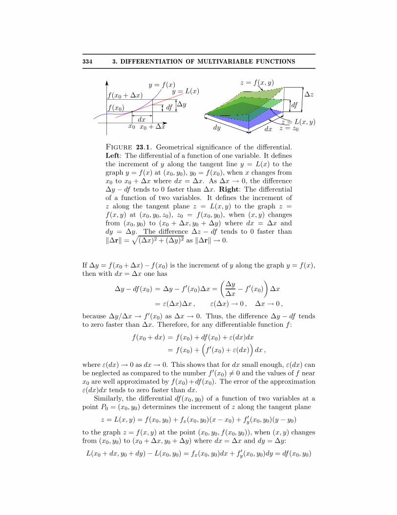
334 3. DIFFERENTIATION OF MULTIVARIABLE FUNCTIONS
y = f(x)y = L(x)
f(x0 + ∆x)
∆yf(x0) df
dxx0 x0 + ∆x
z = f(x, y)
∆z
df
z = L(x, y)z = z0dxdy
Figure 23.1. Geometrical significance of the differential.Left: The differential of a function of one variable. It definesthe increment of y along the tangent line y = L(x) to thegraph y = f(x) at (x0, y0), y0 = f(x0), when x changes fromx0 to x0 + ∆x where dx = ∆x. As ∆x → 0, the difference∆y − df tends to 0 faster than ∆x. Right: The differentialof a function of two variables. It defines the increment ofz along the tangent plane z = L(x, y) to the graph z =f(x, y) at (x0, y0, z0), z0 = f(x0, y0), when (x, y) changesfrom (x0, y0) to (x0 + ∆x, y0 + ∆y) where dx = ∆x anddy = ∆y. The difference ∆z − df tends to 0 faster than‖∆r‖ =
√
(∆x)2 + (∆y)2 as ‖∆r‖ → 0.
If ∆y = f(x0 + ∆x)− f(x0) is the increment of y along the graph y = f(x),then with dx = ∆x one has
∆y − df(x0) = ∆y − f ′(x0)∆x =
(
∆y
∆x− f ′(x0)
)
∆x
= ε(∆x)∆x , ε(∆x) → 0 , ∆x → 0 ,
because ∆y/∆x → f ′(x0) as ∆x → 0. Thus, the difference ∆y − df tendsto zero faster than ∆x. Therefore, for any differentiable function f :
f(x0 + dx) = f(x0) + df(x0) + ε(dx)dx
= f(x0) +(
f ′(x0) + ε(dx))
dx ,
where ε(dx) → 0 as dx → 0. This shows that for dx small enough, ε(dx) canbe neglected as compared to the number f ′(x0) 6= 0 and the values of f nearx0 are well approximated by f(x0)+df(x0). The error of the approximationε(dx)dx tends to zero faster than dx.
Similarly, the differential df(x0, y0) of a function of two variables at apoint P0 = (x0, y0) determines the increment of z along the tangent plane
z = L(x, y) = f(x0, y0) + fx(x0, y0)(x− x0) + f ′y(x0, y0)(y − y0)
to the graph z = f(x, y) at the point (x0, y0, f(x0, y0)), when (x, y) changesfrom (x0, y0) to (x0 + ∆x, y0 + ∆y) where dx = ∆x and dy = ∆y:
L(x0 + dx, y0 + dy)− L(x0, y0) = fx(x0, y0)dx + f ′y(x0, y0)dy = df(x0, y0)
23. THE DIFFERENTIAL AND TAYLOR POLYNOMIALS 335
as depicted in the right panel of Fig. 23.1. The increment of the functionalong its graph is
∆z = f(x0 + dx, y0 + dy)− f(x0, y0) .
Since f is differentiable and, hence, has a good linear approximation (see(21.3)), the difference ∆z− df(x0, y0) tends to zero faster than the distance
dr =√
(dx)2 + (dy)2 as dr → 0. Therefore, similarly to the one-variablecase, the differential defines the linearization of the function and approx-imates variations of values of the function in a neighborhood of a givenpoint,
f(x0 + dx, y0 + dy) = f(x0, y0) + df(x0, y0) + ε(dx, dy)dr ,
where ε(dx, dy) → 0 as dr =√
(dx)2 + (dy)2 → 0.It is now straightforward to generalize the relation between the differen-
tial and the linearization to functions of any number of variables. Let L(r)be the linearization of a function f at a point r0. Then
L(r0 + dr) = f(r0) + df(r0) .
By differentiability of f (see (21.3)), the differential approximates variationsof values of f in a neighborhood of a given point
f(r0 + dr) = f(r0) + df(r0) + ‖dr‖ε(dr)where the error of the approximation ‖dr‖ε(dr) tends to 0 faster than ‖dr‖because ε(dr) → 0 as dr → 0. In other words, the differential determinesvariations of a differentiable function f under variations dr of its argument,when higher powers ‖dr‖p, p > 1, can be neglected as compared to ‖dr‖.
Example 23.1. Find df(x, y) if f(x, y) =√
1 + x2y. In particular,evaluate df(1, 3) for (dx, dy) = (0.1,−0.2). What is the significance of thisnumber?
Solution: The function has continuous partial derivatives in a neighbor-hood of (1, 3) and hence is differentiable at (1, 3). One has
df(x, y) = f ′x(x, y)dx + f ′
y(x, y)dy =xydx
√
1 + x2y+
x2dy
2√
1 + x2y.
Then
df(1, 3) =3
2dx +
1
4dy = 0.15− 0.05 = 0.1
The number f(1, 3) + df(1, 3) defines the value of the linearization L(x, y)of f at (1, 3) for (x, y) = (1 + dx, 3 + dy). It can be used to approximate
f(1 + dx, 3 + dy) when ‖dr‖ =√
(dx)2 + (dy)2 are small enough (small incomparison with, e.g., ‖dr‖2):
f(1 + dx, 3 + dy) ≈ L(1 + dx, 3 + dy) = f(1, 3) + df(1, 3)
336 3. DIFFERENTIATION OF MULTIVARIABLE FUNCTIONS
In particular, a calculator gives f(1 + 0.1, 3−0.2)− f(1, 3) = 0.09476 whichis to be compared with df(1, 3) = 0.1. Note that in this case (dx)2 = 0.01and (dy)2 = 0.04 are nearly tenfold smaller than dx and dy. �
23.2. Applications to the Error Analysis. If a quantity f depends on sev-eral other quantities, say, x, y, and z, for definitiveness, i.e., f is a functionf(x, y, z). Suppose measurements show that x = x0, y = y0, and z = z0.Since in practice all measurements contain errors, the value f(x0, y0, z0) doesnot have much of practical significance until its error is determined.
For example, the volume of a rectangular box with dimensions x, y, andz is the function of three variables
V (x, y, z) = xyz .
In practice, repetitive measurements give the values of x, y, and z fromintervals
x0 − δx ≤ x ≤ x0 + δx, y0 − δy ≤ y ≤ y0 + δy, z0 − δz ≤ z ≤ z0 + δz,
where r0 = 〈x0, y0, z0〉 are the mean values of the dimensions for all mea-surements, while δr = 〈δx, δy, δz〉 are upper bounds of the absolute errors orthe maximal uncertainties of the measurements. To indicate the maximaluncertainty in the measured quantities, one writes
x = x0 ± δx , y = y0 ± δx , z = z0 ± δz .
Different methods of the length measurement would have different absoluteerror bounds (or maximal uncertainties). In other words, the dimensions x,y, and z and the bounds δx, δy, and δz are all independent variables. Thevalues of the dimensions obtained in each measurement are
x = x0 + dx , y = y0 + dy , z = z0 + dz ,
where the differentials (dx, dy, dz) (or small variations) take their values inthe intervals
−δx ≤ dx ≤ δx, −δy ≤ dy ≤ δy, −δz ≤ dz ≤ δz .
Let Rδ be the rectangular box spanned by all such values of dr = 〈dx, dy, dz〉.The question arises:
Given the mean values r0 = 〈x0, y0, z0〉 and the absolute error bounds δr,what is the absolute error bound of the volume value calculated at r0?
For each particular measurement, the error is
V (r0 + dr)− V (r0) = dV (r0)
assuming that terms tending to 0 faster than ‖dr‖ can be neglected (errorsof measurements are assumed to be small, at least, one wishes so). The

23. THE DIFFERENTIAL AND TAYLOR POLYNOMIALS 337
components of dr are independent variables taking their values in the rect-angular box Rδ. Then the maximal uncertainty of the calculated value ofthe volume is
δV = maxRδ
|dV (r0)| ,
where the maximum is taken over all dr in Rδ. For example, if r0 = 〈1, 2, 3〉is in centimeters and δr = 〈1, 1, 1〉 is in millimeters, then the absolute errorof the volume is
δV = maxRδ
|dV (r0)| = maxRδ
|y0z0 dx + x0z0 dy + x0y0 dz|
= maxRδ
|6dx + 3dy + 2dz| = 0.6 + 0.3 + 0.2 = 1.1 cm3
V = V (r0) ± δV = 6± 1.1 cm3 .
Here the maximum is reached at dx = dy = dz = ±0.1 cm. The aboveanalysis of error bounds can be generalized.
Definition 23.2. (Absolute and Relative Error Bounds).Let f be a quantity that depends on other quantities r = 〈x1, x2, ..., xm〉 sothat f = f(r) is a differentiable function. Suppose that the values xi = ai
are known with the absolute error bounds δxi. Put r0 = 〈a1, a2, ..., am〉,dr = 〈dx1, dx2, ..., dxm〉, and
δf = maxRδ
|df(r0)| , Rδ = {dr | − δxi ≤ dxi ≤ δxi , i = 1, 2, ...,m} .
where the maximum is taken over all the rectangular box Rδ. The numberδf is called the absolute error bound of the value of f at r = r0. If, inaddition, f(r0) 6= 0, then the number
ε =δf
|f(r0)|× 100%
is called the relative error bound of the value of f at r = r0.
In the above example, the relative error bound of the volume measure-ments is ε = (1.1/6)× 100% ≈ 18%. The values of each term in the linearfunction
df(r0) =
m∑
i=1
f ′xi
(r0) dxi
lie in the interval
−|f ′xi
(r0)|δxi ≤ f ′xi
(r0) dxi ≤ |f ′xi
(r0)|δxi , i = 1, 2, ...,m
where the boundary values are reached when dxi = ±δxi. Taking the sumover i in this inequality it is concluded that |df(r0)| attains its maximal valueon Rδ when dxi = δxi for all i for which the coefficient f ′
xi(r0) is positive
338 3. DIFFERENTIATION OF MULTIVARIABLE FUNCTIONS
and dxi = −δxi for all i for which the coefficient f ′xi
(r0) is negative. So theabsolute error bound can be written in the form
δf =
m∑
i=1
|f ′xi
(r0)| δxi.
23.3. Accuracy of a Linear Approximation. Values of a differentiable func-tion f(x) near x0 can be well approximated by its linearization:
f(x0 + dx) ≈ f(x0) + df(x0) = f(x0) + f ′(x0)dx ,
where dx denotes a variation of the variable x near x0. Suppose f is differ-entiable many times. The following questions are of interest.
• Can one estimate the error bound of the linear approximation?• Can one systematically improve an approximation of f near x0?
These questions are answered by the Taylor theorem studied in Calculus Iand II. It asserts that if f(x) has continuous derivatives up to order n on an
interval I containing x0 and f (n+1) exists and is bounded on I, |f (n+1)(x)| ≤Mn+1 for some constant Mn+1, then
f(x) = Tn(x) + εn(x) ,
Tn(x) = f(x0) +f ′(x0)
1!∆x +
f ′′(x0)
2!(∆x)2 + · · ·+ f (n)(x0)
n!(∆x)n ,
|εn(x)| ≤ Mn+1
(n + 1)!|∆x|n+1 , ∆x = x − x0 .(23.1)
The polynomial Tn(x) is called the Taylor polynomial of degree n about x0.The remainder εn(x) determines the absolute error of the nth-order Taylorpolynomial approximation f(x) ≈ Tn(x).
Suppose one wants to approximate the values of a function f in aninterval
I : x0 − δx ≤ x ≤ x0 + δx
for some δx > 0. The function f is assumed to have sufficiently manycontinuous derivatives in this interval. Put
x = x0 + dx , |dx| ≤ δx .
The differential dx determines variations of the argument of f near x0 andδx is the upper bound of these variations. Let us write an explicit form of afew first Taylor polynomials about the point x0 (with x− x0 = dx) and theupper bound of the error of the corresponding approximation of the functionf in the interval I :
T0(x0 + dx) = f(x0) ,
|f(x0 + dx)− T0(x0 + dx)| ≤ M1|dx| , M1 = maxI
|f ′(x)|
The zero-degree Taylor polynomial is a constant T0(x) = f(x0). It approx-imates the values of f in the interval I by the value f(x0). Naturally, the

23. THE DIFFERENTIAL AND TAYLOR POLYNOMIALS 339
maximal error of such an approximation is determined by the maximal slopeM1 of f in the interval I .
A better approximation is obtained if the rate of change of f at x0 istaken into account. This is achieved by the tangent line approximationwhich is also the first-order Taylor polynomial approximation:
T1(x0 + dx) = f(x0) + f ′(x0)dx = f(x0) + df(x0) ,
|f(x0 + dx) − T1(x0 + dx)| ≤ 1
2M2|dx|2 , M2 = max
I|f ′′(x)|(23.2)
Equation (23.2) answers the question about the accuracy of the tangentline approximation. If the second derivative of f is bounded, then the errorof the tangent line approximation decreases quadratically with decreasingthe distance from the point in a neighborhood of which the function isapproximated.
Naturally, an even better approximation can be obtained if, in additionto the slope, the concavity of the approximated function is taken into ac-count. This is done by the second-order Taylor polynomial approximation:
T2(x0 + dx) = f(x0) + f ′(x0)dx +f ′′(x0)
2!(dx)2 ,
|f(x0 + dx) − T2(x0 + dx)| ≤ M3
6|dx|3 , M3 = max
I|f ′′′(x)| .
Now the error of the approximation decreases with decreasing the distance|dx| even faster.
For a constant function, the zero-order Taylor polynomial approximationabout any point is exact (it has no error). For a linear function, the first-order Taylor polynomial approximation about any point is exact becausea linear function is uniquely determined by its value and the slope at apoint. The second-order Taylor polynomial approximation of a quadraticpolynomial about any point is also exact (a quadratic polynomial has aconstant (fixed) concavity and, hence, is uniquely determined by the valueof the concavity and by its value and the slope at a point):
f ′′(x) = af ′(x0) = bf(x0) = c
⇔ f(x) = c + b(x− x0) +1
2a2(x − x0)
2 .
It is not difficult to see that the Taylor polynomial of degree n for a poly-nomial of the same degree about any point coincides with that polynomial.A polynomial of degree n has a constant nth derivative and therefore canbe uniquely reconstructed from the value of f (n)(x) = a (by taking n an-tiderivatives), provided the values of the polynomial and the values of itsderivatives up to order n − 1 are given at a particular point (to determinethe integration constants). The reconstructed polynomial coincides with theTaylor polynomial.
340 3. DIFFERENTIATION OF MULTIVARIABLE FUNCTIONS
Let us introduce shorter (more convenient) notations for Taylor polyno-mials. The differential df can be viewed as the result of the action of theoperator d on a differentiable function f :
d = dxd
dx: f(x) → df(x) = dx
df(x)
dx= f ′(x)dx
that is, the action of d on f means taking the derivative of f at a pointx and multiplying the result by an independent variable dx. A repetitiveaction of the operator d on f produces higher-order differentials of f . Thenth differential of f is defined by the rule
dnf(x) = f (n)(x)(dx)n =
(
dxd
dx
)n
f(x)
where the action of the powers dn on f is understood as successive actionsof the operator d, dnf = dn−1(df), in which the variables dx and x areindependent. For example,
d2f(x) = d(df(x)) = dx∂
∂x
(
f ′(x)dx)
= (dx)2∂
∂xf ′(x) = (dx)2f ′′(x) .
Then the Taylor polynomials about x0 can be written as
Tn(x0 + dx) = f(x0) +1
1!df(x0) +
1
2!d2f(x0) + · · ·+ 1
n!dnf(x0) ,
where x = x0 + dx or dx = x − x0, and n = 1, 2, .... An upper bound oferrors of the nth order Taylor polynomial approximation in the interval I is
|f(x0 + dx)− Tn(x0 + dx)| ≤ Mn+1
(n + 1)!|dx|n+1 ,(23.3)
Mn+1 = maxI
|f (n+1)(x)| .
It is desirable to find a convenient way to estimate the Taylor approximationerror, avoiding the calculation of constants Mn.
An estimate of the Taylor approximation error. Let us estimate first theabsolute error of the linear approximation. Put |dx| ≤ δx and I = [x0 −δx, x0+δx]. Suppose in addition that f ′′′(x) is continuous on I . By the meanvalue theorem (Calculus 1), for any continuously differentiable function g(x)on I there exists a point x∗ between x0 and x0 + dx such that
g(x0 + dx)− g(x0) = g′(x∗)dx ⇒ g(x0 + dx) = g(x0) + g′(x∗)dx .
In particular, set g(x) = f ′′(x) and use |A + B| ≤ |A| + |B| to obtain
|f ′′(x0 + dx)| ≤ |f ′′(x0)|+ |f ′′′(x∗)||dx|≤ |f ′′(x0)|+ M3|δx| , M3 = max
I|f ′′′(x)| .
The latter inequality holds for any dx in the left side. Therefore
M2 = maxI
|f ′′(x)| ≤ |f ′′(x0)| + M3δx
23. THE DIFFERENTIAL AND TAYLOR POLYNOMIALS 341
because |dx| ≤ δx. For small enough variations of dx (small enough δx), thesecond term in the right side is much smaller than the first one so that M2
can be approximated by |f ′′(x0)|: M2 ≈ |f ′′(x0)|. The absolute error of thelinear approximation can therefore be estimated as
ε1 = |f(x0 + dx)− T1(x0 + dx)| = |f(x0 + dx)− f(x0) − df(x0)|
≤ M2
2|dx|2 ≈ |f ′′(x0)|
2|dx|2 =
1
2|d2f(x0)| ,
ε1 ≈ εes1 =
1
2|d2f(x0)| .
Here εes1 is an estimate of the absolute error of the linear approximation of
f near x0.Similarly by setting g(x) = f (n+1)(x) and assuming that f has suffi-
ciently many continuous derivatives, the constant Mn+1 in Eq. (23.3) isshown to satisfy the condition
Mn+1 ≤ |f (n+1)(x0)|+ Mn+2δx .
For small enough δx, the constant Mn+1 can be approximated by the de-rivative |f (n+1)(x0)|. It follows from (23.3) that the absolute error of theTaylor polynomial approximation can be estimated as
εn = |f(x0 + dx)− Tn(x0 + dx| ≈ εesn(23.4)
εesn =
|f (n+1)(x0)|(n + 1)!
|dx|n+1 =|dn+1f(x0)|
(n + 1)!
The right side of Eq. (23.4) is the term that defines the next order of theTaylor polynomial approximation. If the current approximation is accurate,then a “correction” to it is expected to be small.
This observation can be quantified by estimating the relative error ofthe Taylor approximation
εn =|f(x)− Tn(x)|
|f(x)| × 100% , x = x0 + dx
The top of this ratio is approximated by εesn , while in the denominator one
can use
(23.5) f(x0 + dx) ≈ Tn(x0 + dx)
so that
(23.6) εesn =
|dn+1f(x0)|(n + 1)!|Tn(x0 + dx)| × 100% .
The number εesn is easier to calculate than εn. It is expected to be close to
εn whenever the next term in the Taylor expansion is much smaller thanthe previous one. For example, the linear approximation is expected to be

342 3. DIFFERENTIATION OF MULTIVARIABLE FUNCTIONS
accurate if the term quadratic in dx in the Taylor polynomial approximationis small as compared to the linear one:
(23.7)1
2|d2f(x0)| � |df(x0)| or
|d2f(x0)|2|df(x0)|
� 1 ,
where � stands for “much less”, and the absolute value is needed becausethe values of the first and second differential may be positive or negative.In this case, the relative error and its estimate
(23.8) ε1 ≈ εes1 =
|d2f(x0)|2|f(x0) + df(x0)|
× 100% .
are small.It should be understood that a rigorous bound on the error is given in
the Taylor theorem (23.3). The proposed criteria can be used to estimatethe error by order of magnitude. If, for example, the ratio (23.7) is 0.1or less (one can say, 0.1 � 1), then the next (second) order approximationwould only change the approximate value of the function in the next decimalplace as compared to the first order approximation.
To illustrate the above error analysis, let us estimate the number e0.6
using several Taylor polynomial approximations about 0. So, put
f(x) = ex , x0 = 0 , dx = 0.6 .
Let us write first six terms of the Taylor expansion and calculate their values(up to d5f(x0)). Since f ′(x) = ex = f(x) so that f (n)(0) = 1,
e0.6 ≈ 1 + dx +(dx)2
2+
(dx)3
6+
(dx)4
24+
(dx)5
120= 1 + 0.6 + 0.18 + 0.036 + 0.0054 + 0.000648
= 1.822058
The exact value (rounded to the same decimal place) is 1.822119. Let uscompare the exact and approximate values of the relative errors for a fewTaylor approximations, keeping two first significant digits:
εes0 = 60% , εes
1 = 11% , εes2 = 2.0% , εes
3 = 0.30% , εes4 = 0.036%
ε0 = 45% , ε1 = 12% , ε2 = 2.3% , ε3 = 0.34% , ε4 = 0.039%
So, the estimate of the relative error is not far off, εesn ≈ εn.
So, the Taylor polynomial approximations provide a systematic way toapproximate a function in a neighborhood of a point if the function hassufficiently many continuous derivatives in that neighborhood. It is thereforedesirable to develop an analogous method for functions of several variables.
Remark. There are differentiable functions that cannot be approximatedby Taylor polynomials at some points. For example, the function
f(x) = exp(
− 1
x2
)
, x 6= 0; f(0) = 0 ,
23. THE DIFFERENTIAL AND TAYLOR POLYNOMIALS 343
is differentiable at x = 0 any number of times (as it is at any other point).Using the definition of the derivative as the limit, it is not difficult to showrecursively for n = 1, 2, ... that
f (n)(0) = 0 ⇒ dnf(0) = 0 , n = 1, 2, ... ,
(this is left to the reader as an exercise). Therefore all Taylor polynomialsfor f about x = 0 identically vanish in any neighborhood of x = 0. Onother hand, the function is not zero for a non-zero value of its argument.Hence, f(x) cannot be approximated by Taylor polynomials about x = 0. Ofcourse, Taylor approximations exist about any x0 6= 0 because dnf(x0)) 6= 0for all n if x0 6= 0.
23.4. Taylor Polynomials of Two Variables. Let f be a function of twovariables x and y and the differentials dx and dy be another two independentvariables. By the analogy with the one-variable case, the differential df isviewed as the result of the action of the operator d on f :
df(x, y) =
(
dx∂
∂x+ dy
∂
∂y
)
f(x, y) = dxf ′x(x, y) + dyf ′
y(x, y) .
The operator d has the same properties as the differential (e.g., the productand quotient rules):
d(f + g) = df + dg , d(fg) = dfg + fdg , d
(
f
g
)
=dfg − fdg
g2
for any two differentiable functions f and g (g 6= 0 in the quotient rule).
Definition 23.3. Suppose that f has continuous partial derivatives upto order n. The quantity
dnf(x, y) =
(
dx∂
∂x+ dy
∂
∂y
)n
f(x, y)
is called the nth order differential of f , where the action of powers dn onf is defined successively dnf = dn−1(df) and the variables dx, dy, x, and yare viewed as independent when taking partial derivatives.
The differential dnf is a function of 4 variables dx, dy, x, and y. Forexample,
d2f =
(
dx∂
∂x+ dy
∂
∂y
)2
f =
(
dx∂
∂x+ dy
∂
∂y
)
(dxf ′x + dyf ′
y)
=
(
(dx)2∂
∂x+ dxdy
∂
∂y
)
f ′x +
(
dxdy∂
∂x+ (dy)2
∂
∂y
)
f ′y
= f ′′xx(dx)2 + 2f ′′
xydxdy + f ′′yy(dy)2
By continuity of the partial derivatives, the order of differentiation is irrele-vant (Clairaut’s theorem), f ′′
xy = f ′′yx. The numerical coefficients at each of

344 3. DIFFERENTIATION OF MULTIVARIABLE FUNCTIONS
the terms are binomial coefficients: (a+b)2 = a2 +2ab+b2. Similarly, usingthe binomial coefficients for the cube of the sum
(a + b)3 = a3 + 3a2b + 3ab2 + b3
the third differential is obtained:
d3f = f ′′′xxx(dx)3 + 3f ′′′
xxy(dx)2dy + 3f ′′′xyydx(dy)2 + f ′′′
yyy(dy)3 ,
where Clairaut’s theorem has been used again. The nth differential can bewritten in the form
dnf =
n∑
k=0
Bnk
∂nf
∂xn−k∂yk(dx)n−k(dy)k , Bn
k =n!
k!(n − k)!
where Bnk are the binomial coefficients:
(a + b)n =
n∑
k=0
Bnk an−kbk .
Example 23.2. Find d2f if f(x, y) = x2y + y3.
Solution: The function is a polynomial and hence has continuous partialderivatives of any order. In particular,
f ′′xx = 2y
f ′′xy = 2x
f ′′yy = 6y
⇒d2f = f ′′
xx(x, y)(dx)2 + 2f ′′xy(x, y)dxdy + f ′′
yy(x, y)(dy)2
= 2y(dx)2 + 4xdxdy + 6y(dy)2 .
�
Example 23.3. Find dnf if f(x, y) = eax+by where a and b are con-stants.
Solution: Note first that the function is the composition f(x, y) = eu
where u = ax + by. If f(x, y) = g(u) where u is a function of (x, y), then bythe product rule for the operator d
df = g′(u)du , d2f = d(g′(u)du) = g′′(u)(du)2 + g′(u)d2u .
So by successive actions of the operator d, the differentials of f can beexpressed in terms of the differentials of u. In the case considered, u is alinear function and therefore all second partial derivatives are identicallyzero (and so are all higher-order partial derivatives). Therefore dnu = 0 forall n ≥ 2. Or, notice that du = adx + bdy does not depend on (x, y) andhence d2u = d(du) = 0. It is then concluded that
df = eudu ⇒ d2f = eu(du)2
⇒ dnf = eu(du)n = eax+by(adx + bdy)n ,
for all n. �
23. THE DIFFERENTIAL AND TAYLOR POLYNOMIALS 345
Definition 23.4. (Taylor polynomials of two variables)Let f have continuous partial derivatives up to order n. The Taylor polyno-mial of degree n about a point (x0, y0) is
Tn(x, y) = f(x0, y0) +1
1!df(x0, y0) +
1
2!d2f(x0, y0) + · · ·+ 1
n!dnf(x0, y0)
where dx is set to x − x0 and dy to y − y0 after taking the differentials.
The first four Taylor polynomials are
T0(r) = f(r0),
T1(r) = f(r0) + f ′x(r0) dx + f ′
y(r0) dy ,
T2(r) = T1(r) +f ′′xx(r0)
2(dx)2 + f ′′
xy(r0) dxdy +f ′′yy(r0)
2(dy)2,
T3(r) = T2(r) +f ′′′xxx(r0)
6(dx)3 +
f ′′′xxy(r0)
2(dx)2dy
+f ′′′xyy(r0)
2dx(dy)2 +
f ′′′yyy(r0)
6(dy)3 ,
where r = 〈x, y〉, r0 = 〈x0, y0〉, dx = x − x0, and dy = y − y0. Thelinearization of f at r0 coincides with the first-degree Taylor polynomialT1(r).
23.5. Multivariable Taylor Polynomials. For more than two variables, Tay-lor polynomials are defined similarly. Let
r = 〈x1, x2, ..., xm〉 , dr = 〈dx1, dx2, ..., dxm〉 .
Suppose that a function f has continuous partial derivatives up to order n.The nth order differential of f(r) is defined by
dnf(r) =
(
dx1∂
∂x1+ dx2
∂
∂x2+ · · ·+ dxm
∂
∂xm
)n
f(r)
where the variables r and dr are viewed as independent when differentiating.For example,
d2f(r) =
m∑
j=1
m∑
i=1
f ′′xjxi
(r) dxjdxi ,
d3f(r) =
m∑
k=1
m∑
j=1
m∑
i=1
f ′′′xkxjxi
(r) dxkdxjdxi .
Owing to continuity of the partial derivatives and Clairaut’s theorem, someof the terms in these multiple sums are identical. Numerical coefficients atthe equal terms are the multivariable analog of the binomial coefficients thatappear in the expansion of (a1 + a2 + · · ·+ am)n, n = 2, 3, ....
The Taylor polynomial of degree n about a point r0 is
Tn(r) = f(r0) +1
1!df(r0) +
1
2!d2f(r0) + · · ·+ 1
n!dnf(r0)
346 3. DIFFERENTIATION OF MULTIVARIABLE FUNCTIONS
where dr is set to r−r0 after calculating the differentials. Taylor polynomialsare partial sum of the power series:
f(r0) +∞∑
n=1
dnf(r0)
n!, dr = r − r0 ,
which is called the Taylor series for f about a point r0. If the series convergesto f(r) in some neighborhood of r0:
f(r) = f(r0) +
∞∑
n=1
dnf(r0)
n!, dr = r − r0 ,
then the series is called a power (Taylor) series representation of f near r0.
23.6. Multivariable Taylor polynomial approximations.
Theorem 23.1. (Taylor Theorem)Let D be an open ball centered at r0 and let the partial derivatives of afunction f be continuous up to order n on D. Then
f(r) = Tn(r) + εn(r)
and the reminder εn satisfies the condition
|εn(r)| ≤ hn(r)‖r− r0‖n where hn(r) → 0 as r → r0
If n = 1, then T1(r) = L(r) is the linearization of f at r0. The Taylortheorem merely states that a function with continuous partial derivativeshas a good linear approximation. This is a simple consequence of Theorem21.3 (the continuity of partial derivatives ensures differentiability of f at r0,and, hence, the existence of a good linear approximation). For n ≥ 2, itstates that the approximation of f by the Taylor polynomial Tn is a goodapproximation in the sense that the error decreases faster than ‖r − r0‖n.Consequently, the relative error of the approximation
(23.9) εn =|εn(r)||f(r)| × 100% =
|f(r)− Tn(r)||f(r)| × 100%
is expected to get smaller with increasing n for r close to r0 (assuming thatf(r) 6= 0).
So, a practical significance of the Taylor theorem is that higher-orderdifferentials of a function can be used to obtain successively better approxi-mations of values of a function near a point if the function has continuouspartial derivatives of higher orders in a neighborhood of that point.
Example 23.4. Let f(x, y) =√
1 + x2y. Find df(1, 3) and d2f(1, 3)and use them to approximate f(1 + 0.1, 3− 0.2) by the linear and quadraticTaylor polynomials about (1, 3). Compare the results with the exact value(e.g., use a calculator to find it) by finding the relative errors ε1 and ε2.

23. THE DIFFERENTIAL AND TAYLOR POLYNOMIALS 347
Solution: Put (dx, dy) = (0.1,−0.2). It was found in Example 23.1 thatdf(1, 3) = 0.1. The second partial derivatives are obtained by the quotientrule (see f ′
x and f ′y in Example 23.1):
f ′′xx(1, 3) =
y(1 + x2y)1/2 − x2y2(1 + x2y)−1/2
1 + x2y
∣
∣
∣
(1,3)=
3
8
f ′′xy(1, 3) =
2x(1 + x2y)1/2 − x3y(1 + x2y)−1/2
2(1 + x2y)
∣
∣
∣
(1,3)=
5
16
f ′′yy(1, 3) = −x4
4(1 + x2y)−3/2
∣
∣
∣
(1,3)= − 1
32
Therefore
d2f(1, 3) = f ′′xx(1, 3)(dx)2 + 2f ′′
xy(1, 3)dxdy + f ′′yy(1, 3)(dy)2
=3
8(dx)2 +
5
8dxdy − 1
32(dy)2 = −0.01
The linear approximation gives
f(1 + dx, 3 + dy) ≈ f(1, 3) + df(1, 3) = 2 + 0.1 = 2.1 .
The approximation by the quadratic Taylor polynomial about (1, 3) gives
f(1 + dx, 3 + dy) ≈ f(1, 3) + df(1, 3) +1
2d2f(1, 3)
= 2.1− 0.01/2 = 2.095 .
The exact (calculator) value is f(1 + dx, 3 + dy) = 2.0948 rounded to 4decimal places. The relative errors (rounded to two significant digits) of theobtained Taylor approximations are
ε1 =|2.0948− 2.1|
2.0948× 100% = 0.25% ,
ε2 =|2.0948− 2.095|
2.0948× 100% = 0.0095% .
Evidently, the quadratic approximation is better than the linear approxima-tion. �
Just like in the one-variable case, it is desirable to have a simple methodto estimate the relative error of Taylor approximations. The Taylor theoremdoes not allow to do so because the function hn remains unknown. However,if the function has sufficiently many continuous partial derivatives, an upperbound on hn can be obtained.
Suppose that one wishes to approximate a function f in a ball of radiusδ centered at r0:
Bδ : r = r0 + dr , ‖dr‖ ≤ δ .
Let us first consider the two-variable case, r = 〈x, y〉. The following conse-quence of the Taylor theorem can be proved.
348 3. DIFFERENTIATION OF MULTIVARIABLE FUNCTIONS
Corollary 23.1. (Error bound of the linear approximation)Suppose that a function f has continuous partial derivatives in an open diskBδ = {r | ‖r − r0‖ ≤ δ and the second partial derivatives exist and arebounded on Bδ:
|f ′′xx| ≤ M20 , |f ′′
xy| ≤ M11 , |f ′′yx| ≤ M11 , |f ′′
yy| ≤ M02 ,
all points in Bδ. Let T1(r) = L(r) be the linearization of f at r0. Putr = r0 + dr. Then
|f(r)− L(r)| ≤ 1
2
(
M20(dx)2 + 2M11|dxdy|+ M02(dy)2)
≤ M2
2‖dr‖2 ≤ 1
2M2δ
2(23.10)
for all r in D, where M2 = M20 + 2M11 + M02
Inequality (23.10) follows from |dx| ≤ ‖dr‖ and similarly for the variable y.It is the two-variable analog of (23.2) in the one-variable case. If f has morecontinuous partial derivatives, then a two-variable analog of (23.3) can alsobe established from the Taylor theorem.
Corollary 23.2. (Error Bound of Taylor Polynomial Approximations)If, in addition to the hypotheses of Theorem 23.1, the function f has partialderivatives of order n+1 that are bounded on Bδ; that is, there exist numbersMkn+1, k = 0, 1, 2, ..., n + 1, such that
∣
∣
∣
∣
∂n+1f(x, y)
∂xn+1−k∂yk
∣
∣
∣
∣
≤ Mkn+1 , r = r0 + dr , ‖dr‖ ≤ δ .
Then the remainder satisfies
|εn(r)| ≤n+1∑
k=0
Bn+1k Mkn+1
(n + 1)!|dx|n+1−k|dy|k ,
where Bn+1k = (n + 1)!/(k!(n + 1 − k)!) are binomial coefficients.
The upper bound for the error can be simplified a little bit. Note |dx| ≤‖dr‖ and |dy| ≤ ‖dr‖. Hence, |dx|n+1−k|dy|k ≤ ‖dr‖n+1. Making use of thisinequality, one infers that
(23.11) |εn(r0 + dr)| ≤ Mn+1
(n + 1)!‖dr‖n+1,
where the constant Mn+1 =∑n+1
k=0 Bn+1k Mkn+1. Inequality (23.11) is a two-
variable analog of (23.3).There are natural extensions of Corollaries 23.1 and 23.2 to multivariable
functions. In fact, (23.11) remains valid for any number of variables, wherethe calculation of the constant Mn+1 is changed. Finding an upper boundfor the error of Taylor polynomial approximations requires bounds on partialderivatives of f in a neighborhood of a point. This is not generally an easy
23. THE DIFFERENTIAL AND TAYLOR POLYNOMIALS 349
task. So, just like in the one-variable case, one has to establish a simplepractical way to estimate the error of Taylor approximations.
Error estimates for multivariable Taylor approximations. Suppose that fhas sufficiently many continuous partial derivatives in the ball Bδ (intro-duced above). In contrast to the hypotheses of Corollary 23.2, the partialderivatives of order n + 1 are assumed to be not only existing and bounded,but also continuous. The latter implies that all partial derivatives up ordern + 1 are differentiable functions. This, in turns, means that any partialderivative of order n + 1 has a good linear approximation and, hence, itsmaximal value in the ball Bδ differs from its value at r0 by a term propor-tional to the radius δ ≈ ‖dr‖ of the ball (just like in the one-variable case).Therefore, by replacing the upper bounds Mkn+1 by the absolute values ofthe corresponding partial derivatives at r0 in Corollary 23.2, the error boundis changed by terms of order ‖dr‖n+2 which are small as compared to theleading terms of order ‖dr‖n+1 in (23.11), provided, of course, that ‖dr‖ issmall enough.
Hence, just like in the one-variable case, the absolute error of a Taylorpolynomial approximation
f(r0 + dr) = Tn(r0 + dr) + εn(dr)
can be estimated by the (n + 1)th differential:
εn(dr) ≈ εesn (dr) =
|d(n+1)f(r0)|(n + 1)!
A Taylor polynomial approximation is sufficiently accurate if the next termof the Taylor expansion is much smaller than the former one:
|d(n+1)f(r0)|(n + 1)!
� |dnf(r0)|n!
⇒ |d(n+1)f(r0)|(n + 1)|dnf(r0)|
� 1 .
The relative error of the linear approximation for a function with continuoussecond partial derivatives near a point r0 can be estimated as
(23.12) εes1 =
|d2f(r0)|2|f(r0) + df(r0)|
× 100%
If the second differential happens to be identically zero, then the next non-zero (third) differential can be used to access the accuracy of the linearapproximation. Similarly, the relative error (23.9) of the nth order Taylorapproximation (where r = r0 + dr) is estimated as
εesn =
|d(n+1)f(r0)|(n + 1)!|Tn(r0 + dr)| × 100%
provided the function f has continuous partial derivatives up to order n+1.The above analysis is not specific for functions of two variables. So, thegiven estimates of the relative error of Taylor polynomial approximationscan be used for functions of any number of variables.
350 3. DIFFERENTIATION OF MULTIVARIABLE FUNCTIONS
Example 23.5. Find the linear and quadratic Taylor polynomials forthe function f(x, y) =
√2 + xy about the point (x0, y0) = (2, 1). Use the
polynomials to estimate f(3, 1.5). Estimate the relative relative error of theconstant, linear, and quadratic Taylor polynomial approximations. Comparethe estimates with the exact relative error of these approximations.
Solution: Put x = 2 + dx and y = 1 + dy where dx = 1 and dy =0.5. To estimate the relative accuracy of the quadratic Taylor polynomialapproximation, one has to calculate d3f(2, 1). To avoid computing partialderivatives of f(x, y) up to the third order, the following technical trick isused (compare with technicalities in Example 23.4):
f(2 + dx, 1 + dy) = 2√
1 + du , du =1
4(dx + 2dy + dxdy) .
Since powers of du produce powers of dx and dy, the expansion of (1+du)1/2
in powers du gives the needed expansion in powers of dx and dy. So, putg(u) =
√u. Then (1 + du)1/2 = g(1 + du) and
f(2 + dx, 1 + dy) = f(2, 1) + df(2, 1) +1
2d2f(2, 1) +
1
6d3f(2, 1) + · · ·
= 2g(1 + du)
= 2(
g(1) + dg(1) +1
2d2g(1) +
1
6d3g(1) + · · ·
)
= 2 + du − 1
4(du)2 +
1
8(du)3 + · · · ,
where the dots denotes terms (du)4 and higher. These terms can only givecontributions to d4f(2, 1) and higher as du is proportional to dx and dy.The differentials up to order 3 are obtained by comparing the first line ofthe above equalities with the last one written in powers of dx and dy:
(du)2 =1
16
(
(dx)2 + 4dxdy + 4(dy)2 + 2(dx)2dy + 4dx(dy)2 + · · ·)
(du)3 =1
64(dx + 2dy)3 + · · ·
=1
64
(
(dx)3 + 6(dx)2dy + 12dx(dy)2 + 8(dy)3)
+ · · · ,
where again only terms (dx)k(dy)m with n = k + m ≤ 3 (relevant for dnf ,n ≤ 3) were kept; the terms of higher orders are denoted by dots. Collectingterms with n = 1, 2, 3, the needed differentials of f are found:
df(2, 1) =1
4dx +
1
2dy ,
1
2d2f(2, 1) = − 1
64(dx)2 +
3
16dxdy − 1
16(dy)2
1
6d3f(2, 1) =
(dx)3
512− 5(dx)2dy
256− 5dx(dy)2
128+
(dy)3
64
23. THE DIFFERENTIAL AND TAYLOR POLYNOMIALS 351
Therefore the linear and quadratic Taylor polynomials are
T1(x, y) = 2 +1
4(x − 2) +
1
2(y − 1) ,
T2(x, y) = T1(x, y)− 1
64(x− 2)2 +
3
16(x − 2)(y − 1)− 1
16(y − 1)2
The values of the differentials and the successive Taylor approximations (upto the cubic order) are
f(2 + dx, 1 + dy) ≈ f(2, 1) + df(2, 1) +1
2d2f(2, 1) +
1
6d3f(2, 1)
= 2 + 0.5 + 0.0625− 0.015625
= 2.546875
The exact value of the function is f(2 + 1, 1 + 0.5) = 2.549510 (roundedto the same decimal place as the approximate value). The constant, linear,and quadratic Taylor approximations give, respectively, 2, 2.5, and 2.5625for the value of f(3, 1.5). The estimated and exact relative errors of theseapproximations rounded up to two significant digits are
εes0 = 25% , εes
1 = 1.3% , εes2 = 0.61%
ε0 = 27% , ε1 = 1.9% , ε2 = 0.51% , ε3 = 0.10%
Here ε3 is the relative error of the cubic Taylor polynomial approximation(the value of d4f(2, 1) would be needed for its estimation). One can seethat the successive Taylor approximations improve the accuracy of the ap-proximation and the estimates of the errors are close to the exact values.�
Example 23.6. Use the linear approximation or the differential to esti-mate the amount of aluminum in a closed aluminum can with diameter 10cm and height 10 cm if the aluminum is 0.05 cm thick. Estimate the errorof the approximation.
Solution: The volume of a cylinder of radius r and height h is f(h, r) =πhr2. The volume of a closed cylindrical shell (or the can) of thickness δ istherefore
V = f(h + 2δ, r + δ)− f(h, r) ,
where h and r are the internal height and radius of the shell. Put dh =2δ = 0.1 and dr = δ = 0.05. Then V ≈ df(10, 5). One has f ′
h = πr2 andf ′r = 2πhr; hence,
V ≈ df(10, 5) = f ′h(10, 5) dh+ f ′
r(10, 5) dr = 25π dh + 100π dr
= 7.5π cm3 .
To estimate the error of the linear approximation, the value of the sec-ond differential is needed (f is a polynomial and therefore all its partialderivatives of any order are continuous). The second partial derivatives are
352 3. DIFFERENTIATION OF MULTIVARIABLE FUNCTIONS
f ′′hh = 0, f ′′
hr = 2πr, and f ′′rr = 2πh. Therefore the absolute error of the
approximation can be estimated by
εes1 =
1
2|d2f(10, 5)| = 1
2
(
20πdhdr + 20π(dr)2)
= 0.075π cm3
The estimated relative error is
εes1 =
εes1
|df(10, 5)| × 100% =|d2f(10, 5)|2|df(10, 5)| × 100% = 1% .
�
With increasing the number of variables, calculation of higher-order dif-ferentials of a function to find Taylor polynomials might be a technicallytedious problem. In some special cases, however, it can be avoided. Theidea has already been used in Example 23.5 for a function of two variables.The concept is further elucidated by the following example of a function ofthree variables (see also Study Problem 23.2).
Example 23.7. Find T3 for the function f(x, y, z) = sin(xy + z) aboutthe origin.
Solution: The Taylor polynomial T3 in question is a polynomial of degree 3in x, y, and z, which is uniquely determined by the coefficients at monomialsof degree less or equal 3. Put u = xy + z. The variable u is small near theorigin. So the Taylor polynomial approximation for f near the origin isdetermined by the Taylor polynomials for sin u about u = 0. The latter isobtained from the Maclaurin series
sinu = u − 1
6u3 + O(u5) ,
where O(u5) contains only monomials of degree 5 and higher. Since thepolynomial u = xy + z vanishes at the origin, its powers un may containonly monomials of degree n and higher. Therefore T3 is obtained from
u − 16u3 = (xy + z) − 1
6 (xy + z)3
= z + xy − 16
(
z3 + 3(xy)z2 + 3(xy)2z + (xy)3)
by retaining in the latter all monomials up to degree 3, which yields
T3(x, y, z) = z + xy − 1
6z3 .
Evidently, the procedure is far simpler than calculating 19 partial derivatives(up to the third order)! �
23. THE DIFFERENTIAL AND TAYLOR POLYNOMIALS 353
23.7. Study Problems.
Problem 23.1. Find all Taylor polynomials for
P3(x, y) = 1 + 2x − xy + y2 + 4x3 − y2x
about (0, 0). Use this example to find all Taylor polynomials for a genericpolynomial Pk(x, y) of degree k about (0, 0).
Solution: All partial derivatives of P3 of orders higher than 3 vanish iden-tically so dnP3 = 0 for all n > 3. Therefore Tn = T3 for all n > 3. By directcalculation of the differentials dnP3(0, 0) for n = 1, 2, 3:
T0(x, y) = 1 ,
T1(x, y) = 1 + 2x ,
T2(x, y) = 1 + 2x − xy + y2 ,
T3(x, y) = 1 + 2x − xy + y2 + 4x3 − y2x = P3(x, y) .
Similarly, for a generic polynomial Pk, its Taylor polynomials about (0, 0)of degree higher than k coincide with the Taylor polynomial of degree k,Tn = Tk for all n > k, because dnPk = 0 for n > k. Any polynomial is thesum
Pk = Q0 + Q1 + · · ·+ Qk ,
where Qj is a homogeneous polynomial of degree j = 0, 1, ..., k; it containsonly monomials of degree j. For example, the given polynomial P3 is
P3 = Q0 + Q1 + Q2 + Q3 ,
Q0 = 1 , Q1 = 2x , Q2 = −xy + y2 , Q3 = 4x3 − y2x .
For n ≤ k, the considered example suggests that the following general solu-tion
Tn = Q0 + Q1 + Q2 + · · ·+ Qn , n = 0, 1, 2, ..., k .
Let us prove that this is indeed so.Partial derivatives of a homogeneous polynomial of degree j are homo-
geneous polynomials of degree j − 1, where j ≥ 1. For example, (Q3)′x =
12x2 − y2 and (Q3)′y = −2xy. Consequently, second partial derivatives of
a homogeneous polynomial of degree j are homogeneous polynomials of de-gree j − 2 if j ≥ 2. Clearly, the similar conclusion holds for higher orderderivatives up to order j and all partial derivatives of any order higher thanj vanish identically. Since only a constant homogeneous polynomial doesnot vanish at the origin,
dnQj(0, 0) = 0 for all n 6= j .
Therefore for n ≤ k, the Taylor polynomial of Pk about the origin are
Tn = Q0 + dQ1(0, 0) +1
2!d2Q2(0, 0) + · · ·+ 1
n!dnQn(0, 0) ,
where dx is set to x and dy to y after calculation of the differentials (becausex0 = y0 = 0). So it remains to find dnQn(0, 0) for n ≤ k. A homogeneous
354 3. DIFFERENTIATION OF MULTIVARIABLE FUNCTIONS
polynomial of degree n is the sum of monomials of degree n. Since dn(f +g) = dnf + dng, it is sufficient to find dnQn(0, 0) for Qn = xn−pyp where0 ≤ p ≤ n is an integer. Next note that
∂n
∂xn−q∂yqxn−pyp
∣
∣
∣
(x,y)=(0,0)= (n − p)!p! if q = p
and vanishes otherwise because all the derivatives of yp vanish at y = 0except the pth derivative which is constant and equal to p! (similarly forxn−p). Using the binomial expansion of dn, it is concluded that
Qn(x, y) = xn−pyp ⇒1
n!dnQn(0, 0) = Bn
p
(n − p)!p!
n!(dx)n−p(dy)p = (dx)n−p(dy)p .
Replacing dx and dy by x − x0 = x and y − y0 = y, respectively, it followsthat Taylor polynomials of a polynomial Pk = Q0 + Q1 + · · ·+ Qk, whereQj, j = 1, 2, ..., k, are homogeneous polynomials,
Tn = Q0 + Q1 + · · ·+ Qn , n = 0, 1, ..., k .
In particular, for the given polynomial P3, its Taylor polynomials about theorigin are T0 = 1, T1 = T0 − 2x, T2 = T1 − xy + y2, and Tk = P3 for k ≥ 3.�
Problem 23.2. Find T1, T2 and T3 for f(x, y, z) = (1+xy)/(1+x+y2+z3)about the origin.
Solution: The function f is a rational function. It is therefore sufficientto find a suitable Taylor polynomial for the function (1+x+y2 + z3)−1 andthen multiply it by the polynomial 1 + xy, retaining only monomials up tothe degree 3. Put u = x + y2 + z3. Then
(1 + u)−1 = 1 − u + u2 − u3 + O(u4)
(as a geometric series), where O(u4) contains monomials of degree 4 andhigher. Note that, for n ≥ 4, the terms un contain only monomials of degree4 and higher in variables x, y, and z and, hence, can be omitted. Up to thedegree 3, one has u2 = x2 + 2xy2 + · · · and u3 = x3 + · · · . Therefore,
(1 + xy)(1− u + u2 − u3) = (1 + xy)(1− x− y2 − z3 + x2 + 2xy2 − x3 + · · · )
and carrying out the multiplication and arranging the monomials in theorder of increasing degrees one infers:
T1(x, y, z) = 1 − x ,
T2(x, y, z) = T1(x, y, z) + x2 + xy − y2 ,
T3(x, y, z) = T2(x, y, z)− x3 − x2y + 2xy2 − z3 .
�
23. THE DIFFERENTIAL AND TAYLOR POLYNOMIALS 355
Problem 23.3. (Multivariable Taylor and Maclaurin series)Suppose that a function f has continuous partial derivatives of any orderand the reminder in the Taylor polynomial approximation f = Tn−1 + εn
near r0 converges to zero as n → ∞, i.e., εn → 0. Then the function can berepresented by the Taylor series about a point r0:
f(r) = f(r0) +
∞∑
n=1
1
n!dnf(r0)
where dr is set to r−r0 after calculating the differentials. The Taylor seriesabout r0 = 0 is called the Maclaurin series. Find the Maclaurin series off(x, y) = sin(xy2) and the set in which it converges.
Solution: Since the argument of the sine is the polynomial xy2, theMaclaurin series of f can be obtained from the Maclaurin series of sinuby setting in it u = xy2. From Calculus II,
f(r) = sin u =
∞∑
n=1
(−1)n+1
(2n − 1)!u2n−1 =
∞∑
n=1
(−1)n+1
(2n − 1)!x2n−1y4n−2 .
Since the Maclaurin series for sin u converges for all u, the above seriesconverges for all (x, y). �
23.8. Exercises.1–7. Find the differential df of each of the following functions:
1. f(x, y) = x3 + y3 − 3xy(x− y) ;2. f(x, y) = y cos(x2y) ;3. f(x, y) = sin(x2 + y2) ;4. f(x, y, z) = x + yz + yexyz ;5. f(x, y, z) = ln(xxyyzz) ;6. f(x, y, z) = y/(1 + xyz) ;
7. f(r) =√
a2 − ‖r‖2 where a is a constant and r = 〈x1, x2, ..., xm〉 .
8. Four positive numbers, each less than 100, are rounded and then multi-plied together. Use the differential to estimate the maximum possible errorin the computed product that might result from the rounding.9. A boundary stripe 10 cm wide is painted around a rectangle whose di-mensions are 50 m by 100 m. Use differentials to approximate the number ofsquare meters of paint in the stripe. Use the second differential to estimatethe error bound of the approximation.10. A rectangle has sides of x = 6 and y = 8 meters. Use differentials toestimate the change of the length of the diagonal and the area of the rec-tangle if x is increased by 2 cm and y is decreased by 5 cm. Use the seconddifferential to estimate the error of the approximation.11. Consider a sector of a disk with radius R = 20 cm and the angleθ = π/3. Use the differential to determine how much should the radius bedecreased in order for the area of the sector to remain the same when the
356 3. DIFFERENTIATION OF MULTIVARIABLE FUNCTIONS
angle is increased by 1◦. Use the second differential to estimate the error ofthe approximation.12. Let the quantities f and g be measured with relative errors Rf and Rg.Show that the relative error the product fg is the sum Rf + Rg.13. Measurements of the radius r and the height h of a cylinder arer = 2.2 ± 0.1 and h = 3.1 ± 0.2 in meters. Find the absolute and rela-tive errors of the volume of the cylinder calculated from these data.14. The adjacent sides of a triangle have the lengths a = 100 ± 2 andb = 200 ± 5 in meters, and the angle between them is θ = 60◦ ± 1◦. Findthe relative and absolute errors in calculation of the length of the third sideof the triangle.15. If R is the total resistance of n resistors, connected in parallel, withresistances Rj, j = 1, 2, ..., n, then R−1 = R−1
1 + R−12 + · · ·R−1
n . If eachresistance Rj is known with a relative error of 0.5%, what is the relativeerror of R?16-18. Use the Taylor theorem and its consequences to find the upperbound of the absolute error of the linear approximation of each of the fol-lowing functions about the origin in the ball of radius R (i.e. for ‖r‖ ≤ R):
16. f(x, y) =√
1 + sin(x + y), R = 12 ;
17. f(x, y) = 1+3x2+y , R = 1 ;
18. f(x, y, z) = ln(1 + x + 2y − 3z), R = 0.1 .
19-24. Find the indicated differentials of a given function:
19. f(x, y) = x − y + x2y , dnf , n = 1, 2, ... ;20. f(x, y) = ln(x + y) , dnf , n = 1, 2, ... ;21. f(x, y) = sin(x) cosh(y) , d3f ;22. f(x, y, z) = xyz , dnf , n = 1, 2, ... ;23. f(x, y, z) = 1/(1 + xyz) , d2f ;24. f(r) = ‖r‖ , df and d2f , where r = 〈x1, x2, ..., xm〉 .
25. Let f(r) = g(u) where u is a linear function of r, u = c + n · r where c
is a constant and n is a constant vector. Show that dnf = g(n)(u)(n · dr)n.26. Let Qn(x, y, z) be a homogeneous polynomial of degree n (it containsonly monomials of degree n). Show that dnQn(x, y, z) = n!Qn(dx, dy, dz).27-29. Find the Taylor polynomial T2 about a specified point P0 and agiven function:
27. f(x, y) = y + x3 + 2xy2 − x2y2, P0 = (1, 1) ;28. f(x, y) = sin(xy), P0 = (π/2, 1) ;29. f(x, y) = xy, P0 = (1, 1) .
30. Let f(x, y) = xy. Use Taylor polynomials T1, T2, and T3 about thepoint (1, 1) to approximate f(1.2, 0.7). Compare the results of the threeapproximations with the exact value of f(1.2, 0.7) by computing the relativeerrors of the approximations (use a calculator value rounded to an appro-priate number of decimal places).31-35. Use the method of Example 23.7 and Study Problem 23.2 to find
23. THE DIFFERENTIAL AND TAYLOR POLYNOMIALS 357
the indicated Taylor polynomials about the origin for each of the followingfunctions:
31. f(x, y) =√
1 + x + 2y, Tn(x, y), n ≤ 2 ;32. f(x, y) = xy
1−x2−y2 , Tn(x, y), n ≤ 4 ;
33. f(x, y, z) = sin(x + 2y + z2), Tn(x, y, z), n ≤ 3 ;34. f(x, y, z) = exy cos(zy), Tn(x, y, z), n ≤ 4 ;35. f(x, y) = ln(1 + x + 2y)/(1 + x2 + y2), Tn(x, y), n ≤ 2.
36-37. Find polynomials of degree 2 to calculate approximate values of thefollowing functions in a region in which x2 +y2 is small as compared with 1:
36. f(x, y) = cos y/ cosx ;
37. tan−1(
1+x+y1−x+y
)
.
38. Find a non-zero polynomial of the smallest degree to approximate alocal behavior of the function cos(x + y + z) − cos(x) cos(y) cos(z) near theorigin.39. Let
g(r) =1
2π
∫ 2π
0f(x0 + r cos θ, y0 + r sin θ)dθ
where f has continuous partial derivatives up to order 4 and x0 and y0 areconstants. Find T4 about r = 0 for g(r).40. Consider the roots z = z(x, y) of the equation F (x, y, z) = z5+xz−y = 0near (1, 2, 1). Use Taylor polynomials T1(x, y) and T2(x, y) about (1, 2)to approximate z(x, y). In particular, calculate the approximations z1 =T1(0.7, 2.5) and z2 = T2(0.7, 2.5) of z(0.7, 2.5). Use a calculator to find thevalues F (0.7, 2.5, z1) and F (0.7, 2.5, z2). Their deviation from 0 determinesan error of the approximations z1 and z2. Which of the approximations ismore accurate? Hint: Use the result of Study Problem 22.1.

358 3. DIFFERENTIATION OF MULTIVARIABLE FUNCTIONS
24. Directional Derivative and the Gradient
24.1. Directional Derivative. Let f be a function of several variables r =〈x1, x2, ..., xm〉. The partial derivative f ′
xi(r0) is the rate of change of f at a
point r0 in the direction of the ith coordinate axis. This direction is definedby the unit vector ei parallel to the corresponding coordinate axis. Let u bea unit vector that does not coincide with any of the vectors ei. What is therate of change of f at r0 in the direction of u? For example, if f(x, y) is theheight of a mountain, where the x and y axes are oriented along the west-to-east and south-to-north directions, respectively, then it is reasonable toask about the slopes, for example, in the southeast or northwest directions.Naturally, these slopes generally differ from the slopes f ′
x and f ′y.
To answer the question about the slope in the direction of a unit vectoru, consider a straight line through r0 parallel to u. Its vector equation is
r(h) = r0 + hu ,
where h is a parameter that labels points of the line. The values of f alongthe line are given by the composition
F (h) = f(r(h)) .
The numbers F (0) and F (h) are the values of f at a given point r0 and thepoint r(h), h 6= 0, that is at the distance |h| from r0 along the line. So theslope is given by the derivative
F ′(0) = limh→0
F (h) − F (0)
h.
Therefore, the following definition is natural.
Definition 24.1. (Directional Derivative).Let f be a function on an open set D. The directional derivative of f atpoint r0 in D in the direction of a unit vector u is the limit
Duf(r0) = limh→0
f(r0 + hu)− f(r0)
h
if the limit exists.
The number Duf(r0) is the rate of change of f at r0 in the direction ofu. A geometrical significance of the directional derivative in the case of two-variable function is illustrated in Fig. 24.1. Suppose that f is a differentiablefunction. By definition,
Duf(r0) =d
dhf(r(h))
∣
∣
∣
h=0, r(h) = r0 + hu .
Since f is a differentiable function, the chain rule applies to compute thederivative. In the case of functions of two variables, the parametric equationsof the line through (x0, y0) and parallel to a unit vector u = 〈u1, u2〉 are
x(h) = x0 + hu1 , y(h) = y0 + hu2 .
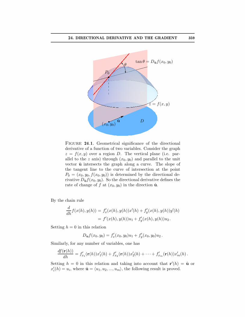
24. DIRECTIONAL DERIVATIVE AND THE GRADIENT 359
P0
θtan θ = Duf(x0, y0)
z = f(x, y)
u(x0, y0)
D
Figure 24.1. Geometrical significance of the directionalderivative of a function of two variables. Consider the graphz = f(x, y) over a region D. The vertical plane (i.e. par-allel to the z axis) through (x0, y0) and parallel to the unitvector u intersects the graph along a curve. The slope ofthe tangent line to the curve of intersection at the pointP0 = (x0, y0, f(x0, y0)) is determined by the directional de-rivative Duf(x0, y0). So the directional derivative defines therate of change of f at (x0, y0) in the direction u.
By the chain rule
d
dhf(x(h), y(h)) = f ′
x(x(h), y(h))x′(h) + f ′y(x(h), y(h))y′(h)
= f ′(x(h), y(h))u1 + f ′y(x(h), y(h))u2 .
Setting h = 0 in this relation
Duf(x0, y0) = f ′x(x0, y0)u1 + f ′
y(x0, y0)u2 .
Similarly, for any number of variables, one has
df(r(h))
dh= f ′
x1(r(h))x′
1(h) + f ′x2
(r(h))x′2(h) + · · ·+ f ′
xm(r(h))x′
m(h) .
Setting h = 0 in this relation and taking into account that r′(h) = u orx′
i(h) = ui, where u = 〈u1, u2, ..., um〉, the following result is proved.
360 3. DIFFERENTIATION OF MULTIVARIABLE FUNCTIONS
Theorem 24.1. (Directional derivative)Suppose f is a differentiable function of several variable r = 〈x1, x2, ..., xm〉on an open set D. Then the directional derivative of f at a point r0 in Din the direction of unit vector u = 〈u1, u2, ..., um〉 is
(24.1) Duf(r0) = f ′x1
(r0)u1 + f ′x2
(r0)u2 + · · ·+ f ′xm
(r0)um .
It is important to emphasize that:
If f has partial derivatives at r0, but is not differentiable at r0, then therelation (24.1) is false.
An example is given in Study Problem 24.1. Note that Eq. (24.1) fol-lows from the chain rule, but the mere existence of partial derivatives is notsufficient for the chain rule to hold. Furthermore, Study Problem 24.1 alsoillustrates the following fact:
Even if a function has directional derivatives at a point in every direction, itmay not be differentiable at that point (no good linear approximation existsat that point).
Equation (24.1) provides a convenient way to compute the directional deriv-ative if f is differentiable. In turn, a practical way to check differentiabilityis provided by Theorem 21.3:
Equation (24.1) holds if the function f has partial derivatives in a neighbor-hood of r0 that are continuous at r0.
The existence and continuity of partial derivatives are often easy to es-tablish by analyzing an explicit form of the function in question (in thisregard, recall the discussion of Clairaut’s Theorem 20.1 in Section 20). Ifthe direction in which the rate of change of a function to be determined isspecified by a nonunit vector u, then the corresponding unit vector can beobtained by dividing it by its length ‖u‖, that is, u = u/‖u‖.
Example 24.1. The height of a hill is f(x, y) = (9−3x2−y2)1/2, wherethe x and y axes in the base of the hill are directed from west to east and fromsouth to north, respectively. A hiker is on the hill at a point corresponding tothe point r0 = 〈1, 2〉 in the base. Suppose the hiker is facing in the northwestdirection. What is the slope the hiker sees?
Solution: A unit vector in the plane can always be written in the formu = 〈cosϕ, sinϕ〉, where the angle ϕ is counted counterclockwise from thepositive x axis; that is, ϕ = 0 corresponds to the east direction, ϕ = π/2to the north direction, ϕ = π to the west direction, and so on. So for thenorthwest direction ϕ = 3π/4 and u = 〈−1/
√2, 1/
√2〉 = 〈u1, u2〉. The
24. DIRECTIONAL DERIVATIVE AND THE GRADIENT 361
partial derivatives,
f ′x(x, y) = − 3x
(9 − 3x2 − y2)1/2, f ′
y(x, y) = − y
(9 − 3x2 − y2)1/2,
are continuous functions near the point (1, 2) (as ratios of continuous func-tions) and hence f is differentiable at (1, 2). Since f ′
x(1, 2) = −3/√
2 and
f ′y(1, 2) = −2/
√2, by (24.1), the slope is
Duf(r0) = f ′x(1, 2)u1 + f ′
y(1, 2)u2 = 3/2− 1 = 1/2 .
If the hiker goes northwest, he has to climb up one unit of length per twounits of length forward. �
Example 24.2. Find the directional derivative of f(x, y, z) = x2+3xz+z2y at the point (1, 1,−1) in the direction toward the point (3,−1, 0). Doesthe function increase or decrease in this direction?
Solution: Put r0 = 〈1, 1,−1〉 and r1 = 〈3,−1, 0〉. Then the vector u =r1 − r0 = 〈2,−2, 1〉 points from the point r0 toward the point r1 accordingto the rules of vector algebra. But it is not a unit vector because its lengthis ‖u‖ = 3. So the unit vector in the same direction is
u = 13u = 〈 2
3 ,−23 , 1
3 〉 = 〈u1, u2, u3〉 .
The partial derivatives,
f ′x = 2x + 3z , f ′
y = z2 , f ′z = 3x + 2zy ,
are polynomials and hence continuous everywhere so that f is differentiableeverywhere. Since f ′
x(r0) = −1, f ′y(r0) = 1, and f ′
z(r0) = 1, by Eq. (24.1),the directional derivative is
Duf(r0) = f ′x(r0)u1 + f ′
y(r0)u2 + f ′z(r0)u3 = −2/3 − 2/3 + 1/3 = −1 .
The directional derivative is negative and therefore the function decreases atr0 in the direction toward r1 (the rate of change is negative in that direction).�
24.2. Level sets of a differentiable function. Level sets of a function f oftwo variables (x, y) are defined by the equation f(x, y) = k. The followingquestion is of interest. Under what conditions on the function f is the levelset a curve? The implicit function theorem (Theorem 22.2) allows us toanswer this question.
Let (x0, y0) be a particular point in the considered level set, that is,f(x0, y0) = k. Suppose that f and f ′
y are continuous in an open disk Dcentered at (x0, y0) and f ′
y(x0, y0) 6= 0. Then by Theorem 22.2 (whereF (x, z) = f(x, z)− k, z = y, and r is a one-dimensional vector whose singlecomponent is x) there exists an open interval D = (a, b) that contains x0 (aneighborhood of x0) in which the equation F (x, y) = f(x, y)− k = 0 has aunique solution y = y(x) where y(x) is a continuous function. Therefore thelevel set is the graph y = y(x) of a continuous function in a neighborhood
362 3. DIFFERENTIATION OF MULTIVARIABLE FUNCTIONS
of (x0, y0) or a simple curve. Furthermore, if f is differentiable, then y(x)is differentiable and the level curve is smooth. The level curve is traversedby the vector function r(t) = 〈t, y(t)〉 and r′(t) = 〈1, y′(t)〉 6= 0 (the unittangent vector to the graph exists and is continuous). If f ′
y(x0, y0) = 0 but
f ′x(x0, y0) 6= 0, then the equation f(x, y)− k = 0 can be solved for x = x(y)
where x(y) is continuous in an open interval containing y0. The level setnear (x0, y0) is again a graph of a continuous function, that is, a curve.
Suppose now that f is a differentiable function and has partial deriva-tives that do not vanish simultaneously. Consider a level curve through(x0, y0). The curve is traversed by the vector function r1(t) = 〈t, y(t)〉if f ′
y(x0, y0) 6= 0 or by r2(t) = 〈x(t), t〉 if f ′x(x0, y0) 6= 0. The vectors
T1 = r′1(x0) = 〈1, y′(x0)〉 and T2 = r′2(y0) = 〈x′(y0), 1〉 are tangent tothe curve at the point (x0, y0). By the implicit differentiation formula,
T1 = 〈1, y′(x0)〉 , y′(x0) = −f ′x(x0, y0)
f ′y(x0, y0)
if f ′y(x0, y0) 6= 0
T2 = 〈x′(y0), 1〉 , x′(y0) = −f ′y(x0, y0)
f ′x(x0, y0)
if f ′x(x0, y0) 6= 0 .
In either case, the tangent vectors are orthogonal to the nonzero vector
n = 〈f ′x(x0, y0) , f ′
y(x0, y0)〉whose components are the corresponding partial derivatives of f at (x0, y0)because
n · T1 = f ′x(x0, y0)− f ′
x(x0, y0) = 0 ,
n · T2 = −f ′y(x0, y0) + f ′
y(x0, y0) = 0 .
Note also that the nonzero vector T = 〈−f ′y(x0, y0), f
′x(x0, y0)〉 is tangent to
the level curve bacause it is orthogonal to n:
n · T = −fx(x0, y0)f′y(x0, y0) + fy(x0, y0)f
′x(x0, y0) = 0 .
If the partial derivatives of f are continuous, then the components of thetangent vector T 6= 0 are continuous functions and, hence, the level curveis smooth. Therefore the following consequence of the implicit functiontheorem holds.
Corollary 24.1. Suppose that a function f of two variables (x, y) hascontinuous partial derivatives in an open disk D that do not vanish simul-taneously anywhere in D. Then nonempty level sets f(x, y) = k are smoothcurves in D.
Now consider a level set of a function of three variables f(x, y, z) = k anda point (x0, y0, z0) in it. If f and f ′
z are continuous in an open ball B centeredat (x0, y0, z0), then by Theorem 22.2 (where F = f − k and r = 〈x, y〉) theequation F (x, y, z) = f(x, y, z) − k = 0 has a unique solution z = z(x, y)which is a continuous function in an open disk D centered at (x0, y0). Thus,the level set is the graph z = z(x, y) of a continuous function of two variable,
24. DIRECTIONAL DERIVATIVE AND THE GRADIENT 363
that is, it is a surface (it is obtained by a continuous deformation of an opendisk in a plane). Furthermore, if f is differentiable in B, then the functionz(x, y) is also differentiable in D. In particular, it has the tangent plane ateach point. By the implicit differentiation formula the partial derivatives ofz(x, y) at a point (x0, y0, z0) of the level surface are
z′x(x0, y0) = −f ′x(x0, y0, z0)
f ′z(x0, y0, z0)
, z′y(x0, y0) = −f ′y(x0, y0, z0)
f ′z(x0, y0, z0)
.
Therefore a normal of the tangent plane to the graph z = z(x, y) at a point(x0, y0, z0) is
〈−z′x(x0, y0), −z′y(x0, y0), 1〉 =1
f ′z(x0, y0, z0)
n if f ′z(x0, y0, z0) 6= 0 ,
n = 〈f ′x(x0, y0, z0), f ′
y(x0, y0, z0), f ′z(x0, y0, z0)〉 ;
it is parallel to the nonzero vector n whose components are the correspondingpartial derivatives at (x0, y0, z0).
Just like in the case of functions of two variables, the implicit functiontheorem can be applied to show that a level set of a differentiable functionof three variables is a surface in a neighborhood of each point of the level setif its partial derivatives do not vanish simultaneously anywhere. If f ′
z = 0at a point P0, then the level set near P0 is the graph of a differentiablefunction, x = x(y, z) if f ′
x(P0) 6= 0 or y = y(x, z) if f ′y(P0) 6= 0. The
implicit differentiation formula yields that in each case the vector n is anormal to the tangent plane to the level surface. The details similar tothe case f ′
z(P0) 6= 0 are left to the reader as an exercise. In all cases, anormal vector to a level surface at a point P0 is parallel to the vector whosecomponents are the corresponding partial derivatives at P0 of the function.Therefore, if the partial derivatives are continuous functions that do notvanish simultaneously, then the normal n 6= 0 has continuous componentsalong the surface. Such (level) surfaces are called smooth. So, the followingconsequence of the implicit function theorem holds.
Corollary 24.2. (Level surfaces)Suppose that a function f of three variables (x, y, z) has continuous partialderivatives in an open ball B that do not vanish simultaneously anywhere inB. Then nonempty level sets f(x, y, z) = k are smooth surfaces in B.
24.3. The Gradient and Its Geometrical Significance. The vector whosecomponents are the corresponding partial derivatives of a differentiable func-tion has been shown to provide an important information about the prop-erties of the function. It is therefore convenient to give it a name.
Definition 24.2. (The Gradient).Let f be a differentiable function of several variables r = 〈x1, x2, ..., xm〉 onan open set D and let r0 be a point in D. The vector whose components are
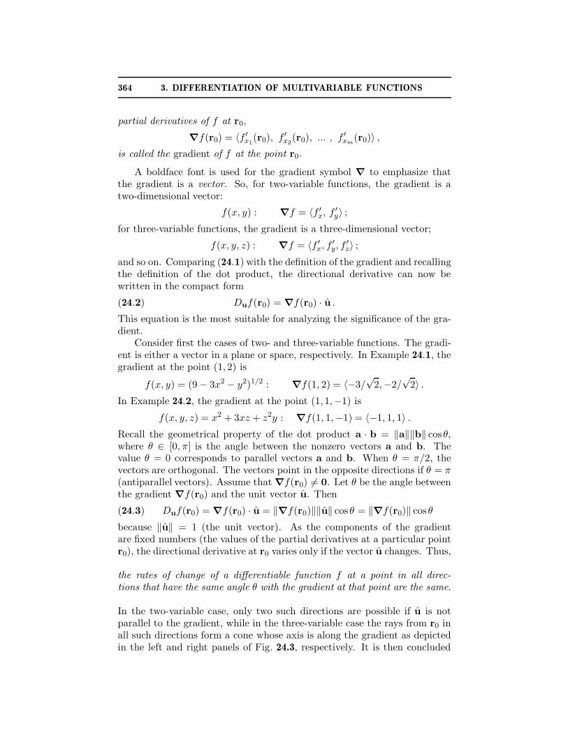
364 3. DIFFERENTIATION OF MULTIVARIABLE FUNCTIONS
partial derivatives of f at r0,
∇f(r0) = 〈f ′x1
(r0), f ′x2
(r0), ... , f ′xm
(r0)〉 ,
is called the gradient of f at the point r0.
A boldface font is used for the gradient symbol ∇ to emphasize thatthe gradient is a vector. So, for two-variable functions, the gradient is atwo-dimensional vector:
f(x, y) : ∇f = 〈f ′x, f ′
y〉 ;
for three-variable functions, the gradient is a three-dimensional vector;
f(x, y, z) : ∇f = 〈f ′x, f ′
y, f′z〉 ;
and so on. Comparing (24.1) with the definition of the gradient and recallingthe definition of the dot product, the directional derivative can now bewritten in the compact form
(24.2) Duf(r0) = ∇f(r0) · u .
This equation is the most suitable for analyzing the significance of the gra-dient.
Consider first the cases of two- and three-variable functions. The gradi-ent is either a vector in a plane or space, respectively. In Example 24.1, thegradient at the point (1, 2) is
f(x, y) = (9− 3x2 − y2)1/2 : ∇f(1, 2) = 〈−3/√
2,−2/√
2〉 .
In Example 24.2, the gradient at the point (1, 1,−1) is
f(x, y, z) = x2 + 3xz + z2y : ∇f(1, 1,−1) = 〈−1, 1, 1〉 .
Recall the geometrical property of the dot product a · b = ‖a‖‖b‖ cosθ,where θ ∈ [0, π] is the angle between the nonzero vectors a and b. Thevalue θ = 0 corresponds to parallel vectors a and b. When θ = π/2, thevectors are orthogonal. The vectors point in the opposite directions if θ = π(antiparallel vectors). Assume that ∇f(r0) 6= 0. Let θ be the angle betweenthe gradient ∇f(r0) and the unit vector u. Then
(24.3) Duf(r0) = ∇f(r0) · u = ‖∇f(r0)‖‖u‖ cosθ = ‖∇f(r0)‖ cosθ
because ‖u‖ = 1 (the unit vector). As the components of the gradientare fixed numbers (the values of the partial derivatives at a particular pointr0), the directional derivative at r0 varies only if the vector u changes. Thus,
the rates of change of a differentiable function f at a point in all direc-tions that have the same angle θ with the gradient at that point are the same.
In the two-variable case, only two such directions are possible if u is notparallel to the gradient, while in the three-variable case the rays from r0 inall such directions form a cone whose axis is along the gradient as depictedin the left and right panels of Fig. 24.3, respectively. It is then concluded
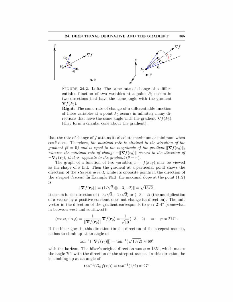
24. DIRECTIONAL DERIVATIVE AND THE GRADIENT 365
y
x
u2
u1
θθP0
∇f
x
y
z
P0u
θ
∇f
Figure 24.2. Left: The same rate of change of a differ-entiable function of two variables at a point P0 occurs intwo directions that have the same angle with the gradient∇f(P0).Right: The same rate of change of a differentiable functionof three variables at a point P0 occurs in infinitely many di-rections that have the same angle with the gradient ∇f(P0)(they form a circular cone about the gradient).
that the rate of change of f attains its absolute maximum or minimum whencos θ does. Therefore, the maximal rate is attained in the direction of thegradient (θ = 0) and is equal to the magnitude of the gradient ‖∇f(r0)‖,whereas the minimal rate of change −‖∇f(r0)‖ occurs in the direction of−∇f(r0), that is, opposite to the gradient (θ = π).
The graph of a function of two variables z = f(x, y) may be viewedas the shape of a hill. Then the gradient at a particular point shows thedirection of the steepest ascent, while its opposite points in the direction ofthe steepest descent. In Example 24.1, the maximal slope at the point (1, 2)is
‖∇f(r0)‖ = (1/√
2)‖〈−3,−2〉‖ =√
13/2 .
It occurs in the direction of 〈−3/√
2,−2/√
2〉 or 〈−3,−2〉 (the multiplicationof a vector by a positive constant does not change its direction). The unitvector in the direction of the gradient corresponds to ϕ ≈ 214◦ (somewhatin between west and southwest):
〈cos ϕ, sinϕ〉 =1
‖∇f(r0)‖∇f(r0) =
1√13
〈−3,−2〉 ⇒ ϕ ≈ 214◦ .
If the hiker goes in this direction (in the direction of the steepest ascent),he has to climb up at an angle of
tan−1(‖∇f(r0)‖) = tan−1(√
13/2) ≈ 69◦
with the horizon. The hiker’s original direction was ϕ = 135◦, which makesthe angle 79◦ with the direction of the steepest ascent. In this direction, heis climbing up at an angle of
tan−1(Duf(r0)) = tan−1(1/2) ≈ 27◦

366 3. DIFFERENTIATION OF MULTIVARIABLE FUNCTIONS
P∇f(P )
f(x, y) = k
f(x, y) = k
∇f∇f ∇f
C
f(x, y, z) = k
∇f(P )
P
Figure 24.3. Left: The gradient at a point P is normalto a level curve f(x, y) = k through P of a function f oftwo variables. Middle: A curve C of steepest descent orascent for a function f has the characteristic property thatthe gradient ∇f is tangent to it. The level curves of f arenormal C. The function f increases most rapidly along Cin the direction of ∇f and f decreases most rapidly alongC in the opposite direction −∇f . Right: The gradient of afunction of three variables is normal to any curve through Pin the level surface f(x, y, z) = k. So, ∇f(P ) is a normal tothe tangent plane through P to the level surface.
with the horizon. The same slope also occurs in the direction ϕ = 214◦ +79◦ = 293◦ at hiker’s current position (see Fig. 24.3 (left panel)).
Next, consider a level set f(x, y) = k of a differentiable function of twovariables. In Section 24.2, it has been shown that level sets are smoothcurves in an open disk D if the partial derivatives f ′
x and f ′y are continuous
and do not vanish simultaneously anywhere in D. Furthermore, it has beenshown that the gradient n= ∇f(x0, y0) 6= 0 at a point (x0, y0) of a levelcurve of f is orthogonal to a tangent vector to the level curve of f at thatpoint. This is often expressed by saying that the gradient of f is alwaysnormal to the level curves of f .
This geometrical property of the gradient is illustrated in the left panel ofFig. 24.3. Recall that a function f(x, y) can be described by a contour map,which is a collection of level curves. Then one can define a curve througha particular point that is normal to all level curves in some neighborhoodof that point. This curve is called the curve of steepest descent or ascentthrough that point. A tangent vector of this curve at any point is parallel tothe gradient at that point. The values of the function increase (or decrease)most rapidly along this curve. If a hiker follows the direction of the gradientof the height, he would go along the path of steepest ascent (or the steepestdescent if he follows the direction opposite to the gradient) as depicted inthe middle panel of Fig. 24.3.
Similarly, the level sets f(r) = k of a function of three variables r =〈x, y, z〉 are smooth surfaces inside an open ball B if the partial derivatives
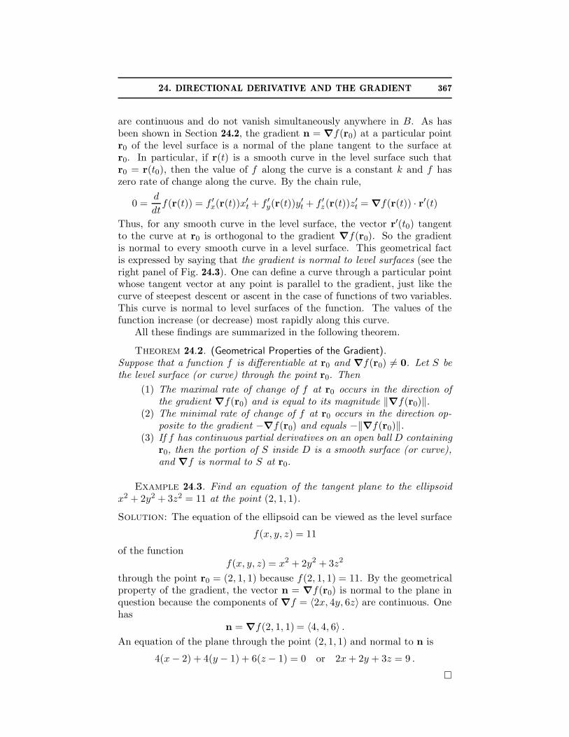
24. DIRECTIONAL DERIVATIVE AND THE GRADIENT 367
are continuous and do not vanish simultaneously anywhere in B. As hasbeen shown in Section 24.2, the gradient n = ∇f(r0) at a particular pointr0 of the level surface is a normal of the plane tangent to the surface atr0. In particular, if r(t) is a smooth curve in the level surface such thatr0 = r(t0), then the value of f along the curve is a constant k and f haszero rate of change along the curve. By the chain rule,
0 =d
dtf(r(t)) = f ′
x(r(t))x′t + f ′
y(r(t))y′t + f ′
z(r(t))z′t = ∇f(r(t)) · r′(t)
Thus, for any smooth curve in the level surface, the vector r′(t0) tangentto the curve at r0 is orthogonal to the gradient ∇f(r0). So the gradientis normal to every smooth curve in a level surface. This geometrical factis expressed by saying that the gradient is normal to level surfaces (see theright panel of Fig. 24.3). One can define a curve through a particular pointwhose tangent vector at any point is parallel to the gradient, just like thecurve of steepest descent or ascent in the case of functions of two variables.This curve is normal to level surfaces of the function. The values of thefunction increase (or decrease) most rapidly along this curve.
All these findings are summarized in the following theorem.
Theorem 24.2. (Geometrical Properties of the Gradient).Suppose that a function f is differentiable at r0 and ∇f(r0) 6= 0. Let S bethe level surface (or curve) through the point r0. Then
(1) The maximal rate of change of f at r0 occurs in the direction ofthe gradient ∇f(r0) and is equal to its magnitude ‖∇f(r0)‖.
(2) The minimal rate of change of f at r0 occurs in the direction op-posite to the gradient −∇f(r0) and equals −‖∇f(r0)‖.
(3) If f has continuous partial derivatives on an open ball D containingr0, then the portion of S inside D is a smooth surface (or curve),and ∇f is normal to S at r0.
Example 24.3. Find an equation of the tangent plane to the ellipsoidx2 + 2y2 + 3z2 = 11 at the point (2, 1, 1).
Solution: The equation of the ellipsoid can be viewed as the level surface
f(x, y, z) = 11
of the function
f(x, y, z) = x2 + 2y2 + 3z2
through the point r0 = (2, 1, 1) because f(2, 1, 1) = 11. By the geometricalproperty of the gradient, the vector n = ∇f(r0) is normal to the plane inquestion because the components of ∇f = 〈2x, 4y, 6z〉 are continuous. Onehas
n = ∇f(2, 1, 1) = 〈4, 4, 6〉 .
An equation of the plane through the point (2, 1, 1) and normal to n is
4(x − 2) + 4(y − 1) + 6(z − 1) = 0 or 2x + 2y + 3z = 9 .
�
368 3. DIFFERENTIATION OF MULTIVARIABLE FUNCTIONS
The gradient of a differentiable function of two variables can be foundif the rates of change of the function in any two non-parallel directions areknown. Similarly, in order to determine the gradient of a function of threevariables, the rates of change in three non-coplanar direction must be known.To understand the claim, fist note that the components of the gradient arepartial derivatives which can be viewed as the directional derivatives alongthe standard basis vectors. The standard basis vectors are perpendicularand, hence, they are non-parallel in a plane (two variables) and non-coplanarin space (three variables). The following example illustrates the concept inthe case of two variables (the multi-variable case is similar).
Example 24.4. Find the maximal rate of change of a differentiable func-tion f of two variables at a point P and the direction in which it occurs ifthe function is decreasing at P in the direction of the vector a = 〈1, 1〉 at a
rate of√
2 and increasing in the direction of the vector b = 〈−1, 2〉 at a rate
of√
5.
Solution: The maximal rate of change occurs in the direction of the gradi-ent at P and is equal to the magnitude of the gradient. Thus, the problemis to find the gradient if
Daf(P ) = −√
2 , Dbf(P ) =√
5 .
The negative sign at√
2 is required as the function is decreasing in thedirection of a. Put ∇f(P ) = 〈X, Y 〉, where the components X and Y ofthe gradient are to be found. Since neither a nor b are unit vectors,
Daf(P ) =1
‖a‖ a ·∇f =1√2(X + Y ) = −
√2 ,
Dbf(P ) =1
‖b‖ b · ∇f =1√5
(−X + 2Y ) =√
5 .
Multiplying the first equation by√
2 and the second equation by√
5, andthen adding the equations, one finds
3Y = 3 ⇒ Y = 1 ; X + Y = −2 ⇒ X = −3 .
The the maximal rate of change of f at P and the direction in which itoccurs are, respectively,
‖∇f‖ = ‖〈−3, 1〉‖ =√
10 , ∇f = 〈−3, 1〉 .
�
It is worth noting that if in this problem a and b are parallel, thenthe problem has no solution. Indeed, two parallel vectors are proportional,a = sb for some real s. Then Daf = ±Dbf (the minus sign occurs if thevectors have opposite directions (anti-parallel vectors)), and the system ofequations for the components of the gradient has no solution.

24. DIRECTIONAL DERIVATIVE AND THE GRADIENT 369
Theorem 24.2 holds for functions of more than three variables as well.Equation (24.2) was obtained for any number of variables, and the repre-sentation of the dot product (24.3) holds in any Euclidean space. Thus, thefirst two properties of the gradient are valid for functions of any number ofvariables. The implicit function theorem holds for any number of variablesso the equation of a level set f(r) = k can be solved with respect one ofthe variables if the gradient does not vanish, e.g., xm = g(x1, ..., xm−1) neara point where the conditions of the theorem are fulfilled (here f ′
xm6= 0).
It can be interpreted as an (m − 1)-dimensional surface embedded in anm-dimensional Euclidean space, which is hard to visualize. To this end, itis only noted that if f has continuous partial derivatives (the componentsof the gradient are continuous functions) and r(t) is a smooth parametriccurve in a level set f(r) = k, then f has a constant value along any suchcurve, and, by the chain rule, it follows that
d
dtf(r(t)) = ∇f(r(t)) · r′(t) = 0 for any t .
At any particular point r0 = r(t0), tangent vectors r′(t0) to all such curvesthrough r0 are orthogonal to a single vector ∇f(r0) 6= 0. So these vectorsform an (m− 1)-dimensional Euclidean space (called a tangent space to thelevel surface at r0), just like all vectors in a plane in three dimensionalEuclidean space are orthogonal to a normal of the plane. In this sense,the third property of the gradient holds for functions of more than threevariables.
Remark. The gradient can be viewed as the result of the action of theoperator ∇ = 〈∂/∂x1, ∂/∂x2, · · · , ∂/∂xm〉 if ∇f is understood in the senseof multiplication of the “vector” ∇ by a scalar f :
∇f =⟨ ∂
∂x1,
∂
∂x2, ...,
∂
∂xm
⟩
f =⟨ ∂f
∂x1,
∂f
∂x1, ...,
∂f
∂x1
⟩
.
With this notation, the operator d introduced to define the differentials ofa function f has a compact form d = dr ·∇. The linearization L(r) of f(r)at r0 and the differentials of f also have a simple form for any number ofvariables:
L(r) = f(r0) + ∇f(r0) · (r− r0) , dnf(r) = (dr ·∇)nf(r) .
24.4. Study Problems.
Problem 24.1. (Differentiability and Directional Derivative)Let f(x, y) = y3/(x2 + y2) if (x, y) 6= (0, 0) and f(0, 0) = 0. Show thatDuf(0, 0) exists for any u, but it is not given by equation (24.1). Show thatthis function is not differentiable at (0, 0). In other words, the existenceof the directional derivative at a point in every direction does not implydifferentiability at that point.
370 3. DIFFERENTIATION OF MULTIVARIABLE FUNCTIONS
Solution: Put u = 〈cos θ, sin θ〉 for 0 ≤ θ < 2π. By the definition of thedirectional derivative
Duf(0, 0) = limh→0
f(h cos θ, h sin θ) − f(0, 0)
h= lim
h→0
h3 sin3 θ
h3= sin3 θ .
In particular, for θ = 0, u = (1, 0), and Duf(0, 0) = f ′x(0, 0) = 0; similarly
for θ = π/2, u = (0, 1), and Duf(0, 0) = f ′y(0, 0) = 1. Therefore
f ′x(0, 0)u1 + f ′
y(0, 0)u2 = sin θ 6= sin3 θ = Duf(0, 0)
that is, the relation (24.1) does not hold.Since the partial derivatives exist, the function is differentiable if the
linear L(x, y) = f ′x(0, 0)x + f ′
y(0, 0)y = y is a good linear approximation tof at the origin. But the limit
lim(x,y)→(0,0)
f(x, y)− L(x, y)
(x2 + y2)1/2= − lim
(x,y)→(0,0)
yx2
(x2 + y2)3/2
does not exist because the limits along straight lines (x, y) = (t, at), t → 0+,
have different values a/(1+a2)3/2, where a is real. So, f is not differentiableat the origin, despite that it has all directional derivatives at the origin. �
Problem 24.2. Suppose that three level surfaces f(x, y, z) = 1, g(x, y, z) =2, and h(x, y, z) = 3 are intersecting along a smooth curve C. Let P bea point on C in whose neighborhood f , g, and h have continuous partialderivatives and their gradients do not vanish at P . Find ∇f · (∇g × ∇h)at P .
Solution: Let v be a tangent vector to C at the point P (it exists be-cause the curve is smooth). By Part (3) of Theorem 24.2, the equationsf(x, y, z) = 1, g(x, y, z) = 2, and h(x, y, z) = 3 define three smooth surfacesin a neighborhood of P . Since C lies in the surface f(x, y, z) = 1, the gradi-ent ∇f(P ) is orthogonal to v. Similarly, the gradients ∇g(P ) and ∇h(P )must be orthogonal to v. Therefore, all the gradients must be in a planeperpendicular to the vector v. The triple product for any three coplanarvectors vanishes, and hence ∇f · (∇g × ∇h) = 0 at P . �
Problem 24.3. (Energy Conservation in Mechanics)Consider Newton’s second law ma = F. Suppose that the force is the gra-dient F = −∇U , where U = U(r). Let r = r(t) be the trajectory satisfyingNewton’s second law. Prove that the quantity E = mv2/2 + U(r), wherev = ‖r′(t)‖ is the speed, is a constant of motion, that is, dE/dt = 0. Thisconstant is called the total energy of a particle. A force that can be repre-sented by the gradient of a function U is called a conservative force, and thefunction U is called a potential energy.
Solution: First, note that v2 = v ·v. Hence, (v2)′ = 2v ·v′ = 2v ·a. Usingthe chain rule,
dU
dt= U ′
xx′(t) + U ′yy
′(t) + U ′zz
′(t) = r′ · ∇U = v · ∇U .

24. DIRECTIONAL DERIVATIVE AND THE GRADIENT 371
It follows from these two relations that
dE
dt=
m
2(v2)′ +
dU
dt= mv · a + v · ∇U = v · (ma− F) = 0
So the total energy is conserved for the trajectory of the motion. �
24.5. Exercises.1. Let f be a differentiable function of two variables. Specify the directionsat a particular point in which the function has no rate of change? Howmany such directions exist if the first partial derivatives do not vanish atthat point? Answer the same questions for a differentiable function of threevariables.2. Let f(x, y) = y if y 6= x2 and f(x, y) = 0 if y = x2. Find Dnf(0, 0) forall unit vectors n. Show that f(x, y) is not differentiable at (0, 0). Is thefunction continuous at (0, 0)?3–8. For each of the following functions, find the gradient and the direc-tional derivative at a specified point P in the direction parallel to a givenvector v. Indicate whether the function increases or decreases in that direc-tion at P .
3. f(x, y) = x2y, P = (1, 2), v = 〈4, 3〉 ;4. f(x, y) = x/(1 + xy), P = (1, 1), v = 〈2, 1〉 ;5. f(x, y, z) = x2y − zy2 + xz2, P = (1, 2,−1), v = 〈1,−2, 2〉 ;6. f(x, y, z) = tan−1(1 + x + y2 + z3), P = (1,−1, 1), v = 〈1, 1, 1〉 ;7. f(x, y, z) =
√x + yz, P = (1, 1, 3), v = 〈2, 6, 3〉 ;
8. f(x, y, z) = (x + y)/z, P = (2, 1, 1), v = 〈2,−1,−2〉 .9–13. Find the maximal and minimal rates of change of each of the followingfunctions at a specified point P and the directions in which they occur. Findthe directions in which the function has zero rate of change at P .
9. f(x, y) = x/y2, P = (2, 1) ;10. f(x, y) = xy, P = (2, 1) ;11. f(x, y, z) = xz/(1 + yz), P = (1, 2, 3) ;12. f(x, y, z) = x sin(yz), P = (1, 2, π/3);13. f(x, y, z) = xyz
, P = (2, 2, 1) .
14. Let f(x, y) = y/(1 + x2 + y). For a number −1 ≤ p ≤ 1, find allunit vectors u along which the rate of change of f at (2,−3) is p times themaximal rate of change of f at (2,−3).15. For the function f(x, y, z) = 1
2x2− 12y2x+z3y at the point P0 = (1, 2,−1)
find:
(i) The maximal rate of change of f and the direction in which itoccurs;
(ii) A direction in which the rate of change is half of the maximal rateof change. How many such directions exist?
(iii) The rate of change in the direction from P0 toward the point P =(3, 1, 1) .
372 3. DIFFERENTIATION OF MULTIVARIABLE FUNCTIONS
16. If f is a differentiable real-valued function of one real variable, andu is a differentiable real-valued function of m real variables, show that∇(f(u(r))) = f ′(u(r))∇u(r), where r = 〈x1, x2, . . . , xm〉.17. Find ∇‖c× r‖2 where c is a constant vector.18. If f is a differentiable real-valued function of two real variables, andu and v are differentiable real-valued functions of m real variables, showthat ∇f(u(r), v(r)) = f ′
u(u(r), v(r))∇u(r)+f ′v(u(r), v(r))∇v(r), where r =
〈x1, x2, . . . , xm〉.19. Find the directional derivative of f(r) = (x/a)2 + (y/b)2 + (z/c)2 ata point r = 〈x, y, z〉 in the direction of r. Find the points at which thisderivative is equal to ‖∇f‖.20. Find the angle between the gradients of f = x/(x2 + y2 + z2) at thepoints (1, 2, 2) and (−3, 1, 0).
21. Let f(x, y, z) = z/√
x2 + y2 + z2. Sketch the level surfaces of the func-tion f and the function ‖∇f‖. What is the significance of the level surfacesof ‖∇f‖? Find the maximal and minimal values of f and ‖∇f‖ in theregion 1 ≤ z ≤ 2.22. Let a curve C be defined as the intersection of the planesin θ(x − x0) − cos θ(y − y0) = 0, where θ is a parameter, and the graphz = f(x, y) of a differentiable function f is differentiable. Find tanα whereα is the angle between the tangent line to C at (x0, y0, f(x0, y0)) and the xyplane.23. Consider the function f(x, y, z) = 2
√z + xy and three points P0 =
(1, 2, 2), P1 = (−1, 4, 1), and P2 = (−2,−2, 2). In which direction is theabsolute value of the rate of change of f at P0 the largest, toward P1 ortoward P2? What is the direction in which f has the largest rate of changeat P0?24. For the function f(x, y, z) = xy + zy + zx at the point P0 = (1,−1, 0)find:
(i) The maximal rate of change;(ii) The rate of change in the direction v = 〈−1, 2,−2)〉 ;(iii) The angle θ between v and the direction in which the maximal rate
of f occurs.
25. Let f(x, y, z) = x/(x2 + y2 + z2)1/2. Find the rate of change of f inthe direction of the tangent vector to the curve r(t) = (〈t, 2t2,−2t2)〉 at thepoint (1, 2,−2).26. Find all points at which the gradient of f = x3 + y3 + z3 − 3xyz hasthe given property:
(i) ∇f is orthogonal to the z axis;(ii) ∇f is parallel to the z axis;(iii) ∇f = 0.
27. Let f(r) = ln ‖r−r0‖, where r0 is a fixed vector. Find points r = 〈x, y, z〉in space where ‖∇f‖ = 1.

24. DIRECTIONAL DERIVATIVE AND THE GRADIENT 373
28–33. Show that each of the following equations define a smooth surfacethrough the specified point P in a neighborhood of P , and find the tangentplane and the normal line to the surface through P :
28. x2 + y2 + z2 = 169, P = (3, 4, 12);29. x2 − 2y2 + z2 + yz = 2, P = (2, 1,−1) ;30. x = tan−1(y/z), P = (π/4, 1, 1);31. z = y + ln(x/z), P = (1, 1, 1) ;
32. 2x/z + 2y/z = 8, P = (2, 2, 1);33. x2 + 4y2 + 3z2 = 5, (1,−1/2,−1) .
34. Find the points of the surface x2 + 2y2 + 3z2 + 2xy + 2zx + 4yz = 8 atwhich the tangent planes are parallel to the coordinate planes.35. Find the tangent planes to the surface x2 + 2y2 + 3z2 = 21 that areparallel to the plane x + 4y + 6z = 0.36. Find the points on the ellipsoid x2/a2 + y2/b2 + z2/c2 = 1 at which thenormal line makes equal angles with the coordinate axes.37. Consider the paraboloid z = x2 + y2.
(i) Give the parametric equations of the normal line through a pointP0 = (x0, y0, z0) on the paraboloid;
(ii) Consider all normal lines through points with a fixed value of z0
(say, z0 = 2). Show that all such lines intersects at one single pointwhich lies on the z−axis and find the coordinates of this point.
38. Find the points on the hyperboloid x2 − y2 + 2z2 = 5 where the normalline is parallel to the line that joints the points (3,−1, 0) and (5, 3, 8).39. Find an equation of the plane tangent to the surface x2 + y2 − 4z2 = 1at a generic point (x0, y0, z0) of the surface.
40. Find the rate of change of the function h(x, y) =√
10 − x2y2 at thepoint P0 = (1, 1) in the direction toward the point P = (−2, 5). Let h(x, y)be the height of a mountain in a neighborhood of P0. Would you be climbingup or getting down when you go from P0 toward P?41. Your Mars rover is caught by a dust storm in mountains. The visibilityis zero. Your current position is P0 = (1, 2). You can escape in the directionof a cave located at P1 = (4,−2) or in the direction of the base locatedat P2 = (17, 14). Which way would you drive to avoid steep climbing ordescending if the height in a neighborhood of P0 can be approximated bythe function h(x, y) = xy + x2?42. You are flying a small aircraft on the planet Weirdo. You have dis-turbed a nest of nasty everything-eating bugs. The onboard radar indicatesthat the concentration of the bugs is C(x, y, z) = 100− x2 − 2y2 − 3z2 andC(x, y, z) = 0 if x2 + 2y2 + 3z2 > 100. If your current position is (2, 3, 1), inwhich direction would you fire a mass-destruction microwave laser to kill asmany poor bugs as possible near you? Find the optimal escape trajectory.43. Suppose that the functions f and g have continuous partial deriva-tives, their gradients do not vanish, and their level curves f(x, y) = 0 and

374 3. DIFFERENTIATION OF MULTIVARIABLE FUNCTIONS
g(x, y) = 0 intersect at some point P0. The rate of change of the function fat P0 along the curve g(x, y) = 0 is a half of its maximal rate of change atP0. What is the angle at which the curves intersect (the angle between thetangent lines)?44. Suppose that the directional derivatives Duf = a and Dvf = b of adifferentiable function f of two variables are known at a particular point P0
for two unit non-parallel vectors u and v that make the angles θ and φ withthe x axis counted counterclockwise from the latter, respectively. Find thegradient of f at P0.45. Three tests of drilling into rock along the directions u = 〈1, 2, 2〉,v = 〈0, 4, 3〉, and w = 〈0, 0, 1〉 yielded that the gold concentration increasesat the rates 3 units per meter, 3 units per meter, and 1 unit per meter,respectively. Assume that the concentration is a differentiable function. Inwhat direction would you drill to maximize the gold yield and at what ratedoes the gold concentration increase in that direction?46. A level surface of a differentiable function f(x, y, z) contains the curvesr1(t) = 〈2+3t, 1−t2, 3−4t+t2〉 and r2(t) = 〈1+t2, 2t3−1, 2t+1〉. Can thisinformation be used to find the tangent plane to the surface at the point(2, 1, 3)? If so, find an equation of the plane.47. Prove that tangent planes to the surface xyz = a3 > 0 and the coordi-nate planes form tetrahedrons of equal volumes.48. Prove the total length of intervals from the origin to the points of in-tersection of tangent planes to the surface
√x+
√y +
√z =
√a, a > 0, with
the coordinate axes is constant.49. Two surfaces are called orthogonal at a point of intersection if the nor-mal lines to the surfaces at that point are orthogonal. Show that the surfacesx2 + y2 + z2 = r2, x2 + y2 = z2 tan2 φ, and y cos θ = x sin θ are pairwise or-thogonal at their points of intersection for any values of the constants r > 0,0 < φ < π, and 0 ≤ θ < 2π.50. Find the directional derivative of f(x, y, z) in the direction of the gradi-ent of g(x, y, z). Assume that the gradients ∇f and ∇g do not vanish andhave continuous components. What is the geometrical significance of thisderivative?51. Find the angle at which the cylinder x2 + y2 = a2 intersects the surfacebz = xy at a generic point of intersection (x0, y0, z0).52. A ray of light reflects from a mirrored surface at a point P just as itwould reflect from the mirrored plane tangent to the surface at P (if thelight travels along a vector u, then the reflected light travels along a vectorobtained from u by reversing the direction of the component parallel to thenormal to the surface). Show that the light coming parallel to the z axisfrom above the xy plane will be focused by the parabolic mirror az = x2+y2,a > 0, to a single point. Find its coordinates. This property of parabolicmirrors is used to design telescopes. Conversely, if a point light source is putinto the focus of a parabolic mirror, then the light that is coming out if thesource and reflected by the mirror forms a beam parallel to the symmetryaxis of the mirror. This property is used to design flashlights.
25. MAXIMUM AND MINIMUM VALUES 375
25. Maximum and Minimum Values
25.1. Critical Points of Multivariable Functions. Positions of local maximaand minima of a one-variable function play an important role when analyzingan overall behavior of the function. In Calculus I, it was shown how thederivatives can be used to find local maxima and minima. Here this analysisis extended to multivariable functions.
The following notation will be used. An open ball of radius δ centeredat a point r0 is denoted Bδ = {r | ‖r− r0‖ < δ}; that is, it is a set of pointswhose distance from r0 is less than δ > 0. A neighborhood Nδ(r0) of a pointr0 in a set D is a set of common points of D and Bδ; that is, Nδ(r0) containsall points in D whose distance from r0 is less than δ.
Definition 25.1. (Absolute and Local Maxima or Minima).A function f on a set D is said to have a local maximum at r0 if thereis a neighborhood Nδ(r0) such that f(r0) ≥ f(r) for all r in Nδ(r0). Thenumber f(r0) is called a local maximum value. If there is a neighborhoodNδ(r0) such that f(r0) ≤ f(r) for all r in Nδ(r0), then f is said to have alocal minimum at r0 and the number f(r0) is called a local minimum value.If the inequality f(r0) ≥ f(r) or f(r0) ≤ f(r) holds for all points r in thedomain of f , then f has an absolute maximum or absolute minimum at r0,respectively.
Minimal and maximal values are also called extremum values. In the one-variable case, Fermat’s theorem asserts that if a differentiable function has alocal extremum at x0, then its derivative vanishes at x0. The tangent line tothe graph of f at x0 is horizontal: y = f(x0) + df(x0) = f(x0) + f ′(x0)dx =f(x0). There is an extension of Fermat’s theorem to the multivariable case.
Theorem 25.1. (Necessary Condition for a Local Extremum)If a differentiable function f has a local extremum at an interior point r0 ofits domain D, then df(r0) = 0 or ∇f(r0) = 0 (all partial derivatives of fvanish at r0).
Proof. Consider a smooth parametric curve r(t) through the point r0 suchthat r(t0) = r0. Then dr(t0) = r′(t0)dt 6= 0 (the curves is smooth and,hence, has a non-zero tangent vector). The function F (t) = f(r(t)) definesthe values of f along the curve. Therefore, F (t) must have a local extremumat t = t0. Since f is differentiable, the differential dF (t0) = F ′(t0)dt existsby the chain rule:
dF (t0) = dr(t0) · ∇f(r0) .
By Fermat’s theorem dF (t0) = 0 and, hence, by the geometrical propertiesof the dot product
dF (t0) = 0 ⇒ dr(t0) · ∇f(r0) = 0 ⇒ dr(t0) ⊥ ∇f(r0)
the tangent vector dr(t0) and the gradient ∇f(r0) are orthogonal for anysmooth curve through r0. But the tangent vector dr(t0) is an arbitrary non-zero vector because the curve is arbitrarily chosen. The only vector that is
376 3. DIFFERENTIATION OF MULTIVARIABLE FUNCTIONS
orthogonal to any vector is the zero vector and the conclusion of the theoremfollows: ∇f(r0) = 0. �
In particular, for a differentiable function f of two variables, this theoremstates that the tangent plane to the graph of f at a local extremum ishorizontal.
A local extremum may occur at a point where the function is not dif-
ferentiable. For example, f(x, y) =√
x2 + y2 is continuous everywhere and
has an absolute minimum at (0, 0). Note that the graph z =√
x2 + y2 is acone with the vertex at the origin. However, the partial derivatives f ′
x(0, 0)and f ′
y(0, 0) do not exist because the derivative of f(x, 0) = |x| does notexists at x = 0, and similarly, the derivative of f(0, y) = |y| does not existsat y = 0.
Definition 25.2. (Critical Points).An interior point r0 of the domain of a function f is said to be a criticalpoint of f if either ∇f(r0) = 0 or the gradient does not exist at r0.
It should be emphasized that a function f does not always achieve a localextreme value at a critical point. In particular, the converse of Theorem 25.1is not true. If the gradient of a function f vanishes at a point, then f maynot have a local extremum at that point. For example, let
f(x, y) = xy .
It is differentiable everywhere and its partial derivatives are f ′x = y and
f ′y = x. They vanish at the origin,
∇f(0, 0) = 0 .
However, the function achieves neither a local maximum value nor a localminimum value at this critical point. Indeed, consider a straight line throughthe origin, x = t, y = at. Then the values of f along the line are
F (t) = f(t, at) = at2 .
So F (t) has a minimum at t = 0 if a > 0 or a maximum if a < 0. Thus, fcannot have a local extremum at (0, 0). The graph z = xy is a hyperbolicparaboloid rotated through an angle π/4 about the z axis (see Example 9.4).It looks like a saddle.
Furthermore, consider
f(x, y) = x3 − x2y .
It follows that
f ′x(x, y) = 3x3 − 2xy , f ′
y(x, y) = −x2 ⇒ ∇f(0, 0) = 0 .
However the values of the function along any straight line through the originx = t cos θ, y = t sin θ do not achieve a local extremum value:
F (t) = f(t cos θ, t sin θ) = cos2 θ(cos θ − sin θ)t3 = at3
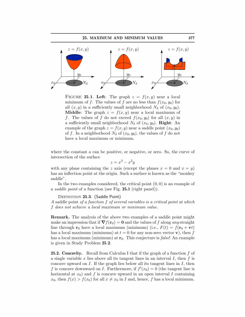
25. MAXIMUM AND MINIMUM VALUES 377
z = f(x, y)
y0
x0 Nδ
z = f(x, y)
y0
x0 Nδ
z = f(x, y)
y0
x0 Nδ
Figure 25.1. Left: The graph z = f(x, y) near a localminimum of f . The values of f are no less than f(x0, y0) forall (x, y) in a sufficiently small neighborhood Nδ of (x0, y0).Middle: The graph z = f(x, y) near a local maximum off . The values of f do not exceed f(x0, y0) for all (x, y) ina sufficiently small neighborhood Nδ of (x0, y0). Right: Anexample of the graph z = f(x, y) near a saddle point (x0, y0)of f . In a neighborhood Nδ of (x0, y0), the values of f do nothave a local maximum or minimum.
where the constant a can be positive, or negative, or zero. So, the curve ofintersection of the surface
z = x3 − x2y
with any plane containing the z axis (except the planes x = 0 and x = y)has an inflection point at the origin. Such a surface is known as the “monkeysaddle”.
In the two examples considered, the critical point (0, 0) is an example ofa saddle point of a function (see Fig. 25.1 (right panel)).
Definition 25.3. (Saddle Point)A saddle point of a function f of several variables is a critical point at whichf does not achieve a local maximum or minimum value.
Remark. The analysis of the above two examples of a saddle point mightmake an impression that if ∇f(r0) = 0 and the values of f along any straightline through r0 have a local maximum (minimum) (i.e., F (t) = f(r0 + vt)has a local maximum (minimum) at t = 0 for any non-zero vector v), then fhas a local maximum (minimum) at r0. This conjecture is false! An exampleis given in Study Problem 25.2.
25.2. Concavity. Recall from Calculus I that if the graph of a function f ofa single variable x lies above all its tangent lines in an interval I , then f isconcave upward on I . If the graph lies below all its tangent lines in I , thenf is concave downward on I . Furthermore, if f ′(x0) = 0 (the tangent line ishorizontal at x0) and f is concave upward in an open interval I containingx0, then f(x) > f(x0) for all x 6= x0 in I and, hence, f has a local minimum.
378 3. DIFFERENTIATION OF MULTIVARIABLE FUNCTIONS
Similarly, f has a local maximum at x0 where f ′(x0) = 0 if it is concavedownward in a neighborhood of x0. If the function f is twice differentiableon I , then it is concave upward if f ′′(x) > 0 on I and it is concave downwardif f ′′(x) < 0 on I . The concavity test can be restated in the form of thesecond differential
d2f(x) = f ′′(x)(dx)2
which is a function of two independent variables x and dx:
d2f(x) > 0, dx 6= 0 ⇒ f is concave upwardd2f(x) < 0, dx 6= 0 ⇒ f is concave downward
Suppose that f ′(x0) = 0, f ′′(x0) 6= 0, and f ′′ is continuous at x0. Recall ifa continuous function is positive (negative) at a particular point, then it ispositive (negative) in a neighborhood of that point. So the continuity of f ′′
ensures that d2f(x) has the same sign as d2f(x0) for all x near x0 and alldx 6= 0. Hence, the graph of f has a fixed concavity in a neighborhood ofx0. Thus, if d2f(x0) < 0 (dx 6= 0), then f has a local maximum at x0 and,if d2f(x0) > 0 (dx 6= 0), then f has a local minimum at x0. It turns outthat this sufficient condition for a function to have a local extremum has anatural extension to functions of several variables.
Theorem 25.2. (Sufficient condition for a local extremum)Suppose that a function f of several variables has continuous second partialderivatives in an open ball containing a point r0 and ∇f(r0) = 0. Then
f has a local maximum at r0 if d2f(r0) < 0,f has a local minimum at r0 if d2f(r0) > 0,
for all dr such that dr 6= 0.
The proof of this theorem is omitted. However, the conclusion of theoremcan be understood as follows. Let r0 be an interior point of the domain of f .Suppose that d2f(r0) > 0 (or d2f(r0) < 0) for all dr 6= 0. If f has continuoussecond partial derivatives, then by Taylor Theorem 23.1, its values near r0
can be approximated by the second Taylor polynomial
f(r0 + dr) = T2(r0 + dr) + ε2(dr)
= f(r0) + df(r0) +1
2d2f(r0) + h2(dr)‖dr‖2 ,
where h2(dr) → 0 as dr → 0. Therefore in a neighborhood Nδ(r0) of asufficiently small radius δ, the sign of the difference between the value ofthe function and the value of its linearization coincides with the sign of thesecond differential d2f(r0):
f(r0 + dr)− f(r0) − df(r0) =1
2d2f(r0) + h2(dr)‖dr‖2 .
Indeed, the error h2‖dr‖2 decreases to zero faster than ‖dr‖2 with decreasing‖dr‖ whereas d2f(r0) decreases as ‖dr‖2 and, hence, |d2f(r0)| > |h2|‖dr‖2
25. MAXIMUM AND MINIMUM VALUES 379
for all 0 < ‖dr‖ < δ and a small enough δ. Neglecting the terms smallerthan ‖dr‖2, it is concluded that
(25.1) f(r0 + dr)− L(r0 + dr) = 12d2f(r0) ,
where L(r0 + dr) = f(r0) + df(r0) is the linearization of f at r0. If, inaddition, r0 is a critical point, that is, df(r0) = 0, then
f(r0 + dr)− f(r0) = 12d2f(r0) .
This equation shows that if d2f(r0) > 0 (or d2f(r0) < 0) for all dr 6= 0, thenat any point in a neighborhood Nδ(r0), the value of f is strictly greater (orstrictly less) than f(r0), and f attains a local maximum value (or a localminimum value) at r0.
Furthermore, the concept of concavity can be extended to the multivari-able case. Let f have continuous second partial derivatives and r0 be aninterior point of the domain of f . Equation (25.1) shows that if d2f(r0) > 0(or d2f(r0) < 0) for all dr 6= 0, then at any point in a neighborhood Nδ(r0),the value of f is strictly greater (or strictly less) than the value of its lin-earization at r0. In particular, in the two-variable case, the graph z = f(x, y)lies above (or below) the tangent plane at (x0, y0) for all (x, y) in a smalldisk centered at (x0, y0). So, this analysis shows that if the second differen-tial d2f(r) is positive (negative) for all r in an open ball B and all dr 6= 0,then the graph z = f(r) over B is concave upward (downward) relative tothe direction of the z axis.
The second differential d2f(r) is a function of two independent variablesr and dr. If second partial derivatives of f are continuous, then the functiond2f is continuous. A continuous function has the property that if it ispositive (negative) at a particular point, then it is positive (negative) in aneighborhood of that point. Therefore if d2f(r0) is positive (negative) forall dr 6= 0 at a critical point r0, then d2f(r) is positive (negative) for alldr 6= 0 and all r in a neighborhood of r0, that is, the graph z = f(r) has afixed concavity in a neighborhood of r0. In the two-variable case, the graphz = f(x, y) near a local maximum at (x0, y0) looks like a paraboloid concavedownward (see Fig. 25.1 (middle panel)). Similarly, the graph z = f(x, y)near a local minimum at (x0, y0) looks like a paraboloid concave upward(see Fig. 25.1 (left panel)).
25.3. Second-Derivative Test. The differential d2f(r0) is a homogeneousquadratic polynomial in the variables dr. Its sign is determined by its coef-ficients which are the second partial derivatives of f at r0. One can pose thequestion: Under what conditions on the second partial derivatives of f at acritical point r0 is the second differential d2f(r0) positive or negative for alldr 6= 0? This question is answered first for functions of two variables. Thegeneral case is studied in the next section.

380 3. DIFFERENTIATION OF MULTIVARIABLE FUNCTIONS
Suppose that a function f of two variable (x, y) has continuous secondpartial derivatives in an open disk centered at r0 = 〈x0, y0〉. Then
d2f(r0) = a(dx)2 + 2cdxdy + b(dy)2 ,
where a = f ′′xx(r0), b = f ′′
yy(r0), and c = f ′′xy(r0) = f ′′
yx(r0) (Clairaut’s theo-rem). The second partial derivatives can be arranged into a 2×2 symmetricmatrix whose diagonal elements are a and b and whose off-diagonal elementsare c. The quadratic polynomial of a variable λ,
P2(λ) = det
(
a − λ cc b − λ
)
= (a − λ)(b− λ)− c2,
is called the characteristic polynomial of the matrix of the second partialderivatives of f at r0.
Theorem 25.3. (Second-Derivative Test).Let r0 be a critical point of a function f . Suppose that the second partialderivatives of f are continuous in an open disk containing r0. Let P2(λ) bethe characteristic polynomial of the matrix of the second partial derivativesof f at r0. Let λi, i = 1, 2, be the roots of P2(λ). Then
(1) If the roots are strictly positive, λi > 0, then f has a local minimumat r0.
(2) If the roots are strictly negative, λi<0, then f has a local maximumat r0.
(3) If the roots do not vanish but have different signs, then f has nei-ther a local maximum nor a local minimum at r0 (in this case, r0
is a saddle point).(4) If at least one of the roots vanishes, then f may have a local maxi-
mum, a local minimum, or none of the above (the second-derivativetest is inconclusive).
A proof of the second-derivative test is given in Section 25.4. The proofshows that the characteristic polynomial P2(λ) always have two real roots(complex roots never occur). The roots may coincide (one real root of mul-tiplicity 2). The roots λ1 and λ2 of the quadratic equation P2(λ) = 0 or
λ2 − (a + b)λ + ab − c2 = 0
are known to satisfy the conditions:
λ1λ2 = ab − c2 , λ1 + λ2 = a + b .
Put D = ab − c2. So, if D < 0, then λ1λ2 < 0 and the roots have differentsigns. By Part (3) of the second-derivative test, r0 is a saddle point. IfD > 0, then the roots have the same sign. Suppose that D > 0. Then eithera > 0 or a < 0. In the first case,
D > 0 ⇒ D
a> 0 ⇒ b >
c2
a> 0 .
25. MAXIMUM AND MINIMUM VALUES 381
Therefore the roots are positive because they have the same sign and theirsum is positive. By Part (1) of the second derivative test, the function hasa local minimum at r0. If a < 0, then
D > 0 ⇒ D
a< 0 ⇒ b <
c2
a< 0 .
Therefore the roots are negative because they have the same sign and theirsum is negative. By Part (2) of the second derivative test, the functionhas a local maximum at r0. Thus, the following consequence of the secondderivative test is established.
Corollary 25.1. Suppose that a function f satisfies the hypothesesof Theorem 25.3. Put D = ab − c2 where a = f ′′
xx(r0), b = f ′′yy(r0), and
c = f ′′xy(r0). Then
(1) If D > 0 and a > 0, then f(r0) is a local minimum.(2) If D > 0 and a < 0, then f(r0) is a local maximum.(3) If D < 0, then r0 is a saddle point of f .(4) If D = 0, then the second-derivative test gives no information about
the nature of the critical point r0.
Example 25.1. Find all critical points of the function
f(x, y) =1
3x3 + xy2 − x2 − y2
and determine whether f has a local maximum, minimum, or saddle at them.
Solution: Critical points. The function is a polynomial, and therefore ithas continuous partial derivatives everywhere of any order. So its criticalpoints are solutions of the system of equations
∇f(x, y) = 0 ⇔{
f ′x = x2 + y2 − 2x = 0
f ′y = 2xy − 2y = 0
It is important to obtain an equivalent system of equations when transform-ing the system ∇f(r) = 0 . It follows from the second equation that eithery = 0 or x = 1. Therefore, the original system of equations is equivalent totwo systems of equations:
{
f ′x = x2 + y2 − 2x = 0x = 1
or
{
f ′x = x2 + y2 − 2x = 0y = 0
.
Solutions of the first system are (1, 1) and (1,−1). Solutions of the secondsystem are (0, 0) and (2, 0). Thus, the function has four critical points.The second-derivative test applies because the function has continuous secondpartial derivatives:
f ′′xx = 2x− 2 , f ′′
yy = 2x − 2 , f ′′xy = 2y.
Critical points (1,±1): The values of the second partial derivatives are:
a = fxx(1,±1) = 0 , b = f ′′yy(1,±1) = 0 , c = f ′′
xy(1,±1) = ±2 .
382 3. DIFFERENTIATION OF MULTIVARIABLE FUNCTIONS
The characteristic equation reads
P2(λ) = (a − λ)(b− λ)− c2 = λ2 − 4 = 0 .
Its roots λ1 = 2 and λ2 = −2 do not vanish and have opposite signs.Therefore, the points (1,±1) are saddle points of the function.Critical point (0, 0): The values of the second partial derivatives are
a = f ′′xx(0, 0) = −2 , b = f ′′
yy(0, 0) = −2 , c = f ′′xy(0, 0) = 0 .
The characteristic equation
P2(λ) = (a − λ)(b − λ) = (−2 − λ)2 = 0
has one negative root of multiplicity 2, that is, λ1 = λ2 = −2 < 0. Thereforef has a local maximum at (0, 0).Critical point (2, 0): The values of the second partial derivatives are
a = f ′′xx(2, 0) = 2 , b = f ′′
yy(2, 0) = 2 , c = f ′′xy(2, 0) = 0 .
The characteristic equation
P2(λ) = (a− λ)(b− λ) = (2− λ)2 = 0
has one positive root of multiplicity 2, λ1 = λ2 = 2 > 0. Therefore thefunction has a local minimum at (2, 0). �
Example 25.2. Investigate the function f(x, y) = ex2−y(5− 2x + y) forextreme values.
Solution: The functions is defined on the whole plane and, as the productof an exponential and a polynomial, it has continuous partial derivatives ofany order. So its critical points are points where its gradient vanishes, andits local extreme values, if any, can be investigated by the second-derivativetest.Critical points. Using the product rule for partial derivatives,
f ′x = ex2−y
(
2x(5− 2x + y) − 2)
= 0 ⇒ x(5 − 2x + y) = 1
f ′y = ex2−y
(
(−1)(5− 2x + y) + 1)
= 0 ⇒ 5 − 2x + y = 1
The substitution of the second equation into the first one yields x = 1. Thenit follows from the second equation that y = −2. So the function has justone critical point (1,−2).Second derivative test. Using the product rule for partial derivatives,
f ′′xx = (f ′
x)′x = ex2−y[
2x(
2x(5 − 2x + y) − 2)
+ 2(5− 2x + y)− 4]
f ′′yy = (f ′
y)′y = ex2−y
[
(−1)(
(−1)(5− 2x + y) + 1)
− 1]
f ′′xy = (f ′
y)′x = ex2−y
[
2x(
(−1)(5− 2x + y) + 1)
+ 2]
The values of the second partial derivatives at the critical point are
a = f ′′xx(1,−2) = −2e3 , b = f ′′
yy(1,−2) = −e3 , c = f ′′xy(1,−2) = 2e3 .
25. MAXIMUM AND MINIMUM VALUES 383
Therefore D = ab − c2 = −2e6 < 0. By Corollary 25.1, the only criticalpoint is a saddle point. The function has no extreme values. �
25.4. Proof of Theorem 25.3. Consider a rotation of the variables (dx, dy):
(dx, dy) = (dx′ cos φ − dy′ sin φ, dy′ cosφ + dx′ sinφ)
Following the proof of Theorem 9.1 (classification of quadric cylinders), thesecond differential is written in the new variables (dx′, dy′) as
d2f(r0) = a(dx)2 + 2cdxdy + b(dy)2 = a′(dx′)2 + 2c′dx′dy′ + b′(dy′)2
a′ = 12
(
a + b + (a− b) cos(2φ) + 2c sin(2φ))
b′ = 12
(
a + b − (a− b) cos(2φ) − 2c sin(2φ))
2c′ = 2c cos(2φ)− (a − b) sin(2φ)
The rotation angle is chosen so that c′ = 0. Put A2 = (a − b)2 + 4c2. Ifcos(2φ) = (a − b)/A and sin(2φ) = 2c/A, then c′ = 0. With this choice,
a′ = 12(a + b + A), b′ = 1
2(a + b − A)
Next note that
a′ + b′ = a + b , a′b′ =1
4((a + b)2 − A2) = ab − c2 .
On the other hand, the roots of the quadratic equation P2(λ) = 0 also satisfythe same conditions
λ1 + λ2 = a + b , λ1λ2 = ab − c2 .
Thus, a′ = λ1, b′ = λ2, and
d2f(r0) = λ1(dx′)2 + λ2(dy′)2
If λ1 and λ2 are strictly positive, then d2f(r0) > 0 for all (dx, dy) 6= (0, 0)and by Theorem 25.2 the function has a local minimum at r0. If λ1 andλ2 are strictly negative, then d2f(r0) < 0 for all (dx, dy) 6= (0, 0) and byTheorem 25.2 the function has a local maximum at r0. If λ1 and λ2 do notvanish but have opposite signs, λ1λ2 < 0, then in a neighborhood of r0, thegraph of f looks like
z = f(r0) + λ1(x′ − x′
0)2 + λ2(y
′ − y′0)2
where the coordinates (x′, y′) are obtained from (x, y) by rotation throughthe angle φ. When λ1 and λ2 have different signs, this surface is a hyperbolicparaboloid (a saddle), and f has neither a local minimum nor maximum.Case (4) is easily proved by examples (see Study Problem 25.3).
384 3. DIFFERENTIATION OF MULTIVARIABLE FUNCTIONS
25.5. Study Problems.
Problem 25.1. Find all critical points of the function f(x, y) =sin(x) sin(y) and determine whether f has a local maximum, minimum, orsaddle at them.
Solution: The function has continuous partial derivative of any order onthe whole plane. So, its critical points are points where the gradient of fvanishes, and the second-derivative test applies to study their nature.Critical points are solutions of the system of equations:
{
f ′x = cos(x) sin(y) = 0
f ′y = sin(x) cos(y) = 0
The first equation is satisfied if either x = π2 + πn or y = πm, where n and
m are integers. So the system is equivalent two systems of equations{
x = π2 + πn
sin(x) cos(y) = 0or
{
y = πm
sin(x) cos(y) = 0
Since sin(π2 + πn) = (−1)n, the second equation of the first system is equiv-
alent to cos y = 0 or y = π2 +πm. The second equation of the second system
is equivalent to sin x = 0 or x = πn. Thus, for any pair of integers n andm, the points
rnm = 〈π2 + πn, π
2 + πm〉 , r′nm = 〈πn, πm〉
are critical points of the function.The second-derivative test has to be applied to each critical point. The secondpartial derivatives are
f ′′xx = − sin(x) sin(y), f ′′
yy = − sin(x) sin(y), f ′′xy = cos(x) cos(y)
For the critical points rnm, one has
a = f ′′xx(rnm) = −(−1)n+m , b = f ′′
yy(rnm) = −(−1)n+m = a ,
c = f ′′xy(rnm) = 0 .
The characteristic equation is (a − λ)2 = 0 and, hence,
λ1 = λ2 = −(−1)n+m .
If n + m is even, then the roots are negative and f(rnm) = 1 is a localmaximum. If n + m is odd, then the roots are positive and f(rnm) = −1 isa local minimum. For the critical points r′nm, one has
a = f ′′xx(r′nm) = 0 , b = f ′′
yy(r′nm) = 0 , c = f ′′xy(r
′nm) = (−1)n+m .
The characteristic equation λ2 − c2 = λ2 − 1 = 0 has two roots λ = ±1 ofopposite signs. Thus, r′nm are saddle points of f . �

25. MAXIMUM AND MINIMUM VALUES 385
Problem 25.2. Let
f(x, y) = x2 + y2 − 2x2y − 4x6y2
(x4 + y2)2if (x, y) 6= (0, 0)
and f(0, 0) = 0. Show that, for all (x, y), the following inequality holds:4x4y2 ≤ (x4+y2)2. Use it and the squeeze principle to conclude that f is con-tinuous. Next, consider a line through (0, 0) and parallel to u = 〈cosϕ, sinϕ〉and the values of f on it:
Fϕ(t) = f(t cosϕ, t sinϕ).
Show that Fϕ(0) = 0, F ′ϕ(0) = 0, and F ′′
ϕ(0) = 2 for all 0 ≤ ϕ ≤ 2π. Thus,f has a minimum at (0, 0) along any straight line through (0, 0). Show thatnevertheless f has no minimum at (0, 0) by studying its value along theparabolic curve (x, y) = (t, t2).
Solution: For any numbers A and B,
0 ≤ (A − B)2 = A2 − 2AB + B2 ⇒ 2AB ≤ A2 + B2 .
Therefore,
4AB = 2AB + 2AB ≤ 2AB + A2 + B2 = (A + B)2 .
By setting A = x4 and B = y2, the said inequality is established:
4x4y2 ≤ (x4 + y2)2 .
The continuity of the last term in f at (0, 0) has to be verified. By the aboveinequality,
0 <4x6y2
(x4 + y2)2≤ 4x6y2
4x4y2= x2 → 0 as (x, y) → (0, 0).
Thus, by the squeeze principle f(x, y) → f(0, 0) = 0 as (x, y) → (0, 0), andf is continuous everywhere. If ϕ = 0 or ϕ = π, that is, the line coincideswith the x axis, (x, y) = (t, 0), one has Fϕ(t) = t2, from which it followsthat Fϕ(0) = F ′
ϕ(0) = 0 and F ′′ϕ(0) = 2. When ϕ is not equal to 0 or π so
that sin ϕ 6= 0, one has
Fϕ(t) = t2 + at3 +bt4
(1 + ct2)2= t2 + at3 + bt4(1 + O(t2)),
a = −2 cos2 ϕ sinϕ, b = −4 cos6 ϕ
sin2 ϕ, c =
cos4 ϕ
sin2 ϕ.
A straightforward differentiation shows that Fϕ(0) = F ′ϕ(0) = 0 and F ′′
ϕ(0) =2 as stated, and Fϕ(t) has an absolute minimum at t = 0, or f attains anabsolute minimum at (0, 0) along any straight line through (0, 0). Never-theless, the latter does not imply that f has a minimum at (0, 0)! Indeed,along the parabola (x, y) = (t, t2), the function f behaves as
f(t, t2) = −t4,
386 3. DIFFERENTIATION OF MULTIVARIABLE FUNCTIONS
which attains an absolute maximum at t = 0. Thus, along the parabola, fhas a maximum value at the origin and hence cannot have a local minimumthere. The problem illustrates the remark given after Definition 25.3. �
Problem 25.3. Suppose that a function f has continuous second partialderivatives and a critical point at which one of the roots of the characteristicequation or both vanish. Prove Part (4) of the second-derivative test bygiving examples of f that has a local maximum, or a local minimum or asaddle at a critical point.
Solution: Consider the function
f(x, y) = x2 + sy4 ,
where s is a number. Since f ′x = 2x and f ′
y = 4sy3, it has one critical point(0, 0). The second partial derivatives at the critical point are
a = f ′′xx(0, 0) = 2 , b = f ′′
yy(0, 0) = 0 , c = f ′′xy(0, 0) = 0 .
Therefore, one of the roots of the characteristic equation is zero:
P2(λ) = −(2 − λ)λ = 0 ⇒ λ1 = 2 , λ2 = 0 .
If s > 0, then f(x, y) ≥ 0 for all (x, y) and f has a minimum at (0, 0). Lets = −1. Then the curves x = ±y2 divide any disk centered at the origininto four sectors with the vertex at the critical point (the origin). In thesectors containing the x axis, f(x, y) ≥ 0, whereas in the sectors containingthe y axis, f(x, y) ≤ 0. Thus, in this case f cannot have a local extremevalue at the critical point. In particular the graph of f has the shape of asaddle. By the similar reasoning, the function
f(x, y) = −(x2 + sy4)
has a maximum value at (0, 0) if s > 0. If s = −1, the graph of f has theshape of a saddle. So, if one of the roots vanishes, then f may have a localmaximum or a local minimum, or a saddle. The same conclusion is reachedwhen λ1 = λ2 = 0 by studying the functions
f(x, y) = ±(x4 + sy4)
along the similar lines of arguments. �
Problem 25.4. For functions of one variable it is impossible for a con-tinuous function to have two local minima (or two local maxima) and nolocal maximum (or no local minimum). However for functions of severalvariables such functions exist. Show that the function
f(x, y) = (y2 − 1)2 + (xy2 − y − 1)2
has two local minima and no local maximum.
25. MAXIMUM AND MINIMUM VALUES 387
Solution: Critical points. The function f is a polynomial and, hence,differentiable everywhere. Therefore its critical points are points where thegradient vanishes:
{
f ′x = 2y2(xy2 − y − 1) = 0
f ′y = 4y(y2 − 1) + 2(2xy − 1)(xy2 − y − 1) = 0
It follows from the first equation that either y = 0 or xy2 − y − 1 = 0. Butthe second equation has no solution if y = 0 because its right side is equalto 2 6= 0 for any x. So, y 6= 0 for any critical point and the above system isequivalent to
{
xy2 − y − 1 = 0y2 − 1 = 0
⇒ (x, y) = (2, 1) , (x, y) = (0,−1) .
Thus, the function has two critical points.Second-derivative test. The second partial derivatives are
f ′′xx = 2y4 ,
f ′′yy = 4(y2 − 1) + 8y2 + 4x(xy2 − y − 1) + 2(2xy − 1)2 ,
f ′′xy = 4y(xy2 − y − 1) + 2y2(2xy − 1) .
Their values at the critical point (2, 1) are
a = f ′′xx(2, 1) = 2 , b = f ′′
yy(2, 1) = 26 , c = f ′′xy(2, 1) = 6
⇒ D = ab − c2 = 52 − 36 = 16 > 0 and a = 2 > 0 .
By Corollary 25.1, the function has a local minimum value at (2, 1). Thevalues of the second partial derivatives at the second critical point are
a = f ′′xx(0,−1) = 2 , b = f ′′
yy(0,−1) = 10 , c = f ′′xy(0,−1) = −2
⇒ D = ab − c2 = 20 − 4 = 16 > 0 and a = 2 > 0 .
By Corollary 25.1, the function has a local minimum value at (2, 1). ByTheorem 25.1 the function f cannot have other critical points and, hence,it has no local maximum value. �
Problem 25.5. (The least square method)Suppose that a scientist has a reason to believe that two quantities x and yare related linearly, y = mx+ b where m and b are unknown constants. Thescientist performs an experiment and collects data as points on the plane(xi, yi), i = 1, 2, ..., N . Since the data contain errors, the points do not lieon a straight line. Let di = yi−(mxi+b) be the vertical deviation of the point(xi, yi) from the line y = mb + x. The method of least squares determinesthe constants m and b by demanding that the sum of squares
∑
d2i attains
its minimal value, thus providing the “best” fit to the data points. Find mand b.

388 3. DIFFERENTIATION OF MULTIVARIABLE FUNCTIONS
Solution: Consider the function f(m, b) =∑N
i=1 d2i . Its critical points
satisfy the equations
f ′b = −2
N∑
i=1
di = 0 , f ′m = −2
N∑
i=1
xidi = 0 ,
because (di)′b = −1 and (di)
′m = −xi. The substitution of di = yi−(mxi +b)
into these equations yields the following system
mN
∑
i=1
xi + bN =N
∑
i=1
yi , mN
∑
i=1
x2i + b
N∑
i=1
xi =N
∑
i=1
xiyi
The solution of this system determines the slope m and the constant b ofthe least square linear fit to the data points:
m =〈x〉〈y〉 − 〈xy〉〈x〉2 − 〈x2〉 , b = 〈y〉 − 〈x〉m ,
where 〈a〉 denotes the mean value of a quantity a:
〈a〉 =1
N
N∑
i=1
ai .
For example 〈xy〉 = (x1y1 + · · ·+xNyN )/N . Note that the second-derivativetest here is not really necessary to conclude that f has a minimum value atthe critical point. Explain why! �
25.6. Exercises.1. Suppose that (0, 0) is a critical point of a function f with continuoussecond partial derivatives. In each case, what can be said about the natureof the critical point:
(i) f ′′xx(0, 0) = −3 , f ′′
xy(0, 0) = 2 , f ′′yy(0, 0) = −2 ;
(ii) f ′′xx(0, 0) = 3 , f ′′
xy(0, 0) = 2 , f ′′yy(0, 0) = 2 ;
(iii) f ′′xx(0, 0) = 1 , f ′′
xy(0, 0) = 2 , f ′′yy(0, 0) = 2 ;
(iv) f ′′xx(0, 0) = 2 , f ′′
xy(0, 0) = 2 , f ′′yy(0, 0) = 2 .
2–27. For each of the following functions, find all critical points and de-termine if they are a relative maximum, a relative minimum, or a saddlepoint:
2. f(x, y) = x2 + (y − 2)2 ;3. f(x, y) = x2 − (y − 2)2 ;4. f(x, y) = x4 − 2x2 − y3 + 3y ;5. f(x, y) = 1
2x2 + 13y3 − xy ;
6. f(x, y) = x2 − xy + y2 − 2x + y ;7. f(x, y) = 1
3x3 + y2 − x2 − 3x − y + 1 ;
8. f(x, y) = x3 + y3 − 3xy ;9. f(x, y) = xy + 50/x + 20/y, x > 0, y > 0 ;
10. f(x, y) = x2 + y2 + 1x2y2 ;
25. MAXIMUM AND MINIMUM VALUES 389
11. f(x, y) = cos(x) cos(y) ;12. f(x, y) = cos x + y2 ;13. f(x, y) = y3 + 6xy + 8x3 ;14. f(x, y) = x3 − 2xy + y2 ;15. f(x, y) = xy(1 − x − y) ;16. f(x, y) = x cos y ;
17. f(x, y) = xy√
1− x2/a2 − y2/b2 ;
18. f(x, y) = (ax + by + c)/√
1 + x2 + y2, a2 + b2 + c2 6= 0 ;
19. f(x, y) = (5x + 7y − 25)e−x2−xy−y2
;20. f(x, y) = sin x + sin y + cos(x + y) ;21. f(x, y) = 1
3x3 + xy2 − x2 − y2 ;
22. f(x, y) = 13y3 + xy + 8
3x3 ;
23. f(x, y) = x2 + xy + y2 − 4 lnx − 10 ln y ;24. f(x, y) = xy ln(x2 + y2) ;25. f(x, y) = x + y + sin(x) sin(y) ;26. f(x, y) = sin(x) + cos(y) + cos(x − y) ;
27. f(x, y) = x − 2y + ln(√
x2 + y2) + 3 tan−1(y/x) .
28-30. Let the function z = z(x, y) be defined implicitly by the givenequation. Use the implicit differentiation to find extreme values of z(x, y):
28. x2 + y2 + z2 − 2x + 2y − 4z − 10 = 0 ;29. x2 + y2 + z2 − xz − yz + 2x + 2y + 2z − 2 = 0 ;30. (x2 + y2 + z2)2 = a2(x2 + y2 − z2) .
31. Find the point on the plane x − y + z = 4 that is closest to the point(1, 2, 3). Hint: minimize the distance from (1, 2, 3) to a generic point of theplane.32. A rectangular box without a lid is to be made from 12 m2 of cardboard.Find the maximum volume of such a box. Hint: express one of the dimen-sions of the box as a function of the others using that the total area of thebox faces is 12 m2 and then maximize the volume.
390 3. DIFFERENTIATION OF MULTIVARIABLE FUNCTIONS
26. Maximum and Minimum Values on a Set
26.1. Second-Derivative Test for Multivariable Functions. Theorem 25.2holds for any number of variables as it is stated and there is a multi-variableanalog of the second derivative test (Theorem 25.3). As in the two-variablecase, the values of the second partial derivatives at a critical point
f ′′xixj
(r0) = Dij
can be arranged into a m × m matrix. By Clairaut’s theorem, this matrixis symmetric Dij = Dji. The polynomial of degree m,
Pm(λ) = det
D11 − λ D12 D13 · · · D1m
D21 D22 − λ D23 · · · D2m
D31 D32 D33 − λ · · · D3m...
......
. . ....
Dm1 Dm2 Dm3 · · · Dmm − λ
,
is called the characteristic polynomial of the matrix of second partial deriva-tives. The following facts are established by methods of linear algebra:
(1) The characteristic polynomial of a real symmetric m × m matrixhas m real roots λ1, λ2,..., λm (a root of multiplicity k is countedk times);
(2) There exists a rotation
dr = 〈dx1, dx2, ..., dxm〉 → dr′ = 〈dx′1, dx2, ..., dx′
m〉 ,
which is a linear homogeneous transformation that preserves thelength ‖dr‖ = ‖dr′‖, such that
d2f(r0) =
m∑
i=1
m∑
j=1
f ′′xixj
(r0)dxidxj =
m∑
i=1
m∑
j=1
Dijdxidxj
= λ1(dx′1)
2 + λ2(dx′2)
2 + · · ·+ λm(dx′m)2
(3) The roots of the characteristic polynomial satisfy the conditions:
λ1 + λ2 + · · ·+ λm = D11 + D22 + · · ·+ Dmm
λ1λ2 · · ·λm = det D
Fact (2) implies that if all roots of the characteristic polynomial are strictlypositive, then d2f(r0) > 0 for all ‖dr‖ = ‖dr′‖ 6= 0 and, hence, f(r0) isa local minimum by Theorem 25.2. Similarly, if all the roots are strictlynegative, then f(r0) is a local maximum. Corollary 25.1 follows from Fact(3) for m = 2. For m > 2 these properties of the roots are insufficient toestablish a multi-variable analog of Corollary 25.1. Fact (3) also impliesthat if detD = 0, then one or more roots are 0. Hence, d2f(r0) = 0 forsome dr 6= 0, and the hypotheses of Theorem 25.2 are not fulfilled.
26. MAXIMUM AND MINIMUM VALUES ON A SET 391
Theorem 26.1. (Second-Derivative Test for m Variables).Let r0 be a critical point of f and suppose that f has continuous second par-tial derivatives in an open ball centered at r0. Let λi, i = 1, 2, ...,m, be rootsof the characteristic polynomial Pm(λ) of the matrix of second derivativesDij = f ′′
xixj(r0).
(1) If all the roots are strictly positive, λi > 0, then f has a localminimum at r0.
(2) If all the roots are strictly negative, λi < 0, then f has a localmaximum at r0.
(3) If two roots have different signs, then f has no local minimum ormaximum at r0.
(4) If some of the roots vanish (or det D = 0), then f may have a localmaximum, or a local minimum, or none of the above (the test isinconclusive).
In case (3) the difference f(r)−f(r0) changes its sign in a neighborhoodof r0. It is an m dimensional analog of a saddle point. In general, rootsof Pm(λ) are found numerically. If some of the roots are guessed, thena synthetic division can be used to reduce the order of the equation. IfPm(λ1) = 0, then there is a polynomial Qm−1 of degree m − 1 such thatPm(λ) = (λ−λ1)Qm−1(λ) so that the other roots satisfy Qm−1(λ) = 0. Thesigns of the roots can also be established by a graphical method (an exampleis given in Study Problem 26.1).
Example 26.1. Investigate the function f(x, y, z) = 13x3 + 1
2y2 + z2 +xy + 2z for extreme values.
Solution: The functions is a polynomial so it has continuous partial deriva-tives of any order everywhere. So its critical points satisfy the equations:
f ′x = x2 + y = 0
f ′y = y + x = 0
f ′z = 2z + 2 = 0
⇔
x2 = xy = −xz = −1
The first equation has two solutions x = 0 and x = 1. So the function hastwo critical points r1 = 〈0, 0,−1〉 and r2 = 〈1,−1,−1〉. The second orderpartial derivatives are
f ′′xx = 2x, f ′′
xy = f ′′yy = 1, f ′′
xz = f ′′yz = 0, f ′′
zz = 2
For the critical point r1, the characteristic polynomial
P3(λ) = det
−λ 1 01 1 − λ 00 0 2 − λ
= (2 − λ)(λ2 − λ − 1)
has the roots 2 and (1±√
5)/2. They do not vanish but have different signs.So r1 is a saddle point of f (no extreme value). For the critical point r2,
392 3. DIFFERENTIATION OF MULTIVARIABLE FUNCTIONS
the characteristic polynomial
P3(λ) = det
2− λ 1 01 1 − λ 00 0 2 − λ
= (2− λ)(λ2 − 3λ + 1)
has positive roots 2 > 0 and (3 ±√
5)/2 > 0. So f(1,−1,−1) = −7/6 is alocal minimum. �
26.2. When the second derivative test is inconclusive. Suppose that a func-tion f has an isolated critical point r0 (that is, a neighborhood of r0 of asmall enough radius has no other critical points). Furthermore, suppose thatf has continuous partial derivatives of sufficiently high orders in a neigh-borhood of r0. Since a local extreme value occurs only at critical points, byDefinition 25.1 f has a local maximum value at r0 if
f(r0 + dr)− f(r0) < 0 for all 0 < ‖dr‖ < δ
for some δ > 0 (δ is the radius of a neighborhood of r0). Similarly, f has alocal minimum value at r0 if
f(r0 + dr)− f(r0) > 0 for all 0 < ‖dr‖ < δ .
By the Taylor theorem, the local behavior of a function near a critical pointr0 is determined by higher order differentials dnf(r0) which are polynomialsin the variable dr:
f(r0 + dr)− f(r0) = 12d2f(r0) + 1
6d3f(r0) + · · ·+ 1n!d
nf(r0) + O(‖dr‖n+1) .
If δ is small enough and d2f(r0) 6= 0 for all dr 6= 0, then the higher orderterms can be neglected and the sign of the difference is determined by thesign of d2f(r0) (all roots of the characteristic polynomial are either positive(a local minimum) or negative (a local maximum)). Suppose that d2f(r0) ≥0 for all dr, but d2f(r0) = 0 for some dr (the case d2f(r0) ≤ 0 can be treatedsimilarly). It is then possible that the difference f(r0 +dr)−f(r0) could benegative for those dr for which d2f(r0) = 0 and the function does not havea local minimum at r0. To determine the sign of the difference, the sign ofhigher order differentials has to be investigated for such dr, that is, the signof d3f(r0) for those dr for which d2f(r0) = 0. If d2f(r0) = d3f(r0) = 0 forsome dr, then the sign of d4f(r0) for these values of dr has to be determined,and so on until the conclusion about the nature of the critical point isreached. It is generally easier to study the concavity of a polynomial thanthat of a general function.
Example 26.2. Show that (0, 0) is a critical point of the function
f(x, y) = (1 + x4 + y2 + y3)1/2 and use a suitable Taylor approximationto determine whether f has a local maximum, minimum, or saddle at (0, 0).
26. MAXIMUM AND MINIMUM VALUES ON A SET 393
Solution: The partial derivatives
f ′x =
2x3
(1 + x4 + y2 + y3)1/2, f ′
y =2y + 3y2
2(1 + x4 + y2 + y3)1/2
vanish at (x, y) = (0, 0). Therefore it is a critical point. Put u = x4+y2+y3.Then
f(x, y) = (1 + u)1/2 = 1 +1
2u + ε(u)u , lim
u→0ε(u) = 0 .
It follows that
f(x, y)− f(0, 0) =1
2u(1 + 2ε(u))
For small enough u, 1 + 2ε(u) > 0 and therefore the sign of this differencein a neighborhood of the critical point is determined by the sign of u. Forsmall enough y 6= 0, y2 + y3 > 0 and, hence, u = x4 + y2 + y3 > 0 forall (x, y) 6= (0, 0) in a neighborhood of (0, 0) and the function has a localminimum at (0, 0). �
The reader can verify that the second derivative test is inconclusive inthis problem by a direct calculation of second partial derivatives. Using theexpansion (1+ u)1/2 = 1 + 1
2u− 18u2 + O(u3), the Taylor polynomials about
the origin can be obtained by retaining the monomials in u and u2 of thedegrees corresponding to the degree of the Taylor polynomial as explainedin Example 23.7 and Study Problem 23.2:
T2 = 1 +1
2y2 , T3 = T2 +
1
2y3 , T4 = T3 +
1
2x4 − 1
8y4 .
It follows from the definition of Taylor polynomials that
1
2!d2f(0, 0) =
1
2(dy)2 ,
1
3!d3f(0, 0) =
1
2(dy)3 ,
1
4!d4f(0, 0) =
1
2(dx)4 − 1
8(dy)4 .
Note that d2f(0, 0) ≥ 0, but d2f(0, 0) = 0 for all dr = 〈dx, 0〉, dx 6= 0.Therefore d2f(0, 0) does not determine the sign of the differencef(r0 + dr) − f(r0) for the critical point r0 = 0 if dr is parallel to the xaxis, and approximations by higher order differentials are needed. Sinced3f(0, 0) also vanishes for dr parallel to the x axis, one has to study the signof d4f(0, 0). The latter happens to be positive for dr = 〈dx, 0〉, dx 6= 0, sothat f(r0 + dr) − f(r0) > 0 for all sufficiently small ‖dr‖ 6= 0. Note thatif the term x4 in the function is replaced by −x4, then the sign of (dx)4 ind4f(0, 0) becomes negative and the function does not have a local extremevalue at (0, 0) because f(r0 + dr)− f(r0) < 0 for dr parallel to the x axis.
In general, the directions of dr along which d2f(r0) = 0 do not coincidewith one (or more) coordinate axes. Such directions are determined by therotation of the coordinate system that brings d2f(r0) to the standard form as
394 3. DIFFERENTIATION OF MULTIVARIABLE FUNCTIONS
noted in the beginning of the section (or in the proof of the second-derivativetest for functions of two variables).
Non-isolated critical points. There are functions whose critical points arenot isolated. Consider the function
f(x, y) = x2(y − 1)2 .
The function is a polynomial (it has continuous partial derivatives of anyorder) and therefore all its critical points are solutions to the system ofequations
{
f ′x = 2x(y − 1)2 = 0
f ′y = 2x2(y − 1) = 0
⇒ (x, y) = (0, p) and (x, y) = (q, 1)
where p and q are any real numbers. Note that the critical points form thelevel set f(x, y) = 0 which consists of two perpendicular lines intersectingat the point (0, 1). The second partial derivatives are
f ′′xx = 2(y − 1)2 , f ′′
yy = 2x2 , f ′′xy = 4x(y − 1)
are continuous and the second derivative test applies. For critical points(0, p), their values are
a = f ′′xx(0, p) = 2(p− 1)2 , b = f ′′
yy(0, p) = 0 , c = f ′′xy(0, p) = 0 .
Therefore D = ab − c2 = 0 and the second-derivative test is inconclusive.Similarly, this test is inconclusive for points (q, 1):
a = f ′′xx(q, 1) = 0 , b = f ′′
yy(q, 1) = 2q2 , c = f ′′xy(q, 1) = 0 ⇒ D = 0 .
However, f(x, y) ≥ 0 for any point and hence in any neighborhood of anycritical point f(x, y) ≥ f(0, p) = 0 and f(x, y) ≥ f(q, 1) = 0 and the functionattains its minimal value at all critical points.
If a function f has a constant value along a curve of its critical pointswhich is, say, a local minimum value, then the graph z = f(r) in a neigh-borhood of a critical point does not look like a concave upward parabo-loid, but rather it resembles a valley in mountains (local minima of theheight are along the valley bottom). Consequently, if the variables dr aresuch that r0 + dr lies on the curve of critical points, then the differencef(r0 +dr)−f(r0) = 0 vanishes for all such dr and so should all the differen-tials dnf(r0) = 0. The analysis based on the sign of higher-order differentialsbecomes inconclusive. However, if the curve of critical points is identified,then variations of the values of the function can be studied in the directionsthat are not tangent to the curve. The sign of higher-order differentials canbe determined for such directions of dr and the nature of critical points canbe established.
In the above example, the critical points r0 = 〈0, p〉 form the y axis.Therefore dr = 〈dx, 0〉, dx 6= 0, is perpendicular to this line and
f(dx, p)− f(0, p) = (dx)2(p− 1)2 > 0 , p 6= 1 .
26. MAXIMUM AND MINIMUM VALUES ON A SET 395
So, the function has a minimum at (0, p), p 6= 1. Similarly, the critical points(q, 1) form a line parallel to the x axis and the vector dr = 〈0, dy〉, dy 6= 0,is perpendicular to it. Then
f(q, 1 + dy)− f(q, 1) = q2(dy)2 > 0 , q 6= 0 .
So, the function has a minimum at (q, 1), q 6= 0. At the point (0, 1), f(dx, 1+dy)−f(0, 1) = (dx)2(dy)2 > 0 and, hence, the function also has a minimum.
In general, if v is a unit vector tangent to a curve formed by criticalpoints at a particular critical point r0, then one has to investigate f(r0+dr)−f(r0) where dr are not independent but subject to the condition v · dr = 0.
26.3. Absolute Maximum and Minimum Values. For a function f of onevariable, the extreme value theorem says that if f is continuous on a closedinterval [a, b], then f has an absolute minimum value and an absolute max-imum value (Calculus I). For example, the function f(x) = x2 on [−1, 2]attains an absolute minimum value at x = 0 and an absolute maximumvalue at x = 2. The function is differentiable for all x and therefore itscritical points are determined by f ′(x) = 2x = 0. So the absolute minimumvalue occurs at the critical point x = 0 inside the interval, while the absolutemaximum value occurs on the boundary of the interval that is not a criticalpoint of f . Thus, to find the absolute maximum and minimum values ofa function f in a closed interval in the domain of f , the values of f mustbe evaluated and compared not only at the critical points but also at theboundaries of the interval.
The situation for multivariable functions is similar. For example, thefunction f(x, y) = x2 + y2 whose arguments are restricted to the squareD = [0, 1]× [0, 1] attains its absolute maximum and minimum values on theboundary of D as shown in the left panel of Fig. 26.1.
Definition 26.1. (Closed Set).A set D in a Euclidean space is said to be closed if it contains all its limitpoints.
Let D be a part of the plane bounded by a simple closed curve C. Recallthat any neighborhood of a limit point of D contains points of D. If a limitpoint of D is not an interior point of D, then it lies on the boundary curveC. So D is closed if it contains its boundary. All points of an open interval(a, b) are its limit points, but, in addition, the boundaries a and b are also itslimit points, so when they are added, a closed set [a, b] is obtained. Similarly,the set in the plane D = {(x, y)|x2 + y2 < 1} has limit points on the circlex2 +y2 = 1 (the boundary of D), which is not in D. By adding these points,a closed set is obtained, x2 + y2 ≤ 1.
Definition 26.2. (Bounded Set).A set D in a Euclidean space is said to be bounded if it is contained in someball.
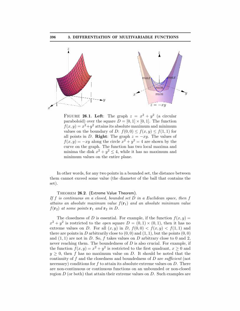
396 3. DIFFERENTIATION OF MULTIVARIABLE FUNCTIONS
x
y
z
11
x y
z
z = −xy
min
min
max max
Figure 26.1. Left: The graph z = x2 + y2 (a circularparaboloid) over the square D = [0, 1]× [0, 1]. The functionf(x, y) = x2+y2 attains its absolute maximum and minimumvalues on the boundary of D: f(0, 0) ≤ f(x, y) ≤ f(1, 1) forall points in D. Right: The graph z = −xy. The values off(x, y) = −xy along the circle x2 + y2 = 4 are shown by thecurve on the graph. The function has two local maxima andminima the disk x2 + y2 ≤ 4, while it has no maximum andminimum values on the entire plane.
In other words, for any two points in a bounded set, the distance betweenthem cannot exceed some value (the diameter of the ball that contains theset).
Theorem 26.2. (Extreme Value Theorem).If f is continuous on a closed, bounded set D in a Euclidean space, then fattains an absolute maximum value f(r1) and an absolute minimum valuef(r2) at some points r1 and r2 in D.
The closedness of D is essential. For example, if the function f(x, y) =x2 + y2 is restricted to the open square D = (0, 1)× (0, 1), then it has noextreme values on D. For all (x, y) in D, f(0, 0) < f(x, y) < f(1, 1) andthere are points in D arbitrarily close to (0, 0) and (1, 1), but the points (0, 0)and (1, 1) are not in D. So, f takes values on D arbitrary close to 0 and 2,never reaching them. The boundedness of D is also crucial. For example, ifthe function f(x, y) = x2 + y2 is restricted to the first quadrant, x ≥ 0 andy ≥ 0, then f has no maximum value on D. It should be noted that thecontinuity of f and the closedness and boundedness of D are sufficient (notnecessary) conditions for f to attain its absolute extreme values on D. Thereare non-continuous or continuous functions on an unbounded or non-closedregion D (or both) that attain their extreme values on D. Such examples are

26. MAXIMUM AND MINIMUM VALUES ON A SET 397
given in Calculus I and functions of a single variable may always be viewedas a particular case of functions of two or more variables: f(x, y) = g(x).
The minimum and maximum values of a function f on a set D will bedenoted, respectively, by minD f and maxD f . One writes
f(r1) = maxD
f and f(r2) = maxD
f ,
if the absolute maximum and minimum occur, respectively, at r1 and r2. Bythe extreme value theorem, it follows that the points r1 and r2 are eithercritical points of f (because local extrema always occur at critical points) orlie on the boundary of D. So, to find the absolute minimum and maximumvalues of a continuous function f on a closed, bounded set D, one has to
Step 1. Find the values of f at the critical points of f in the interior of D.Step 2. Find the extreme values of f on the boundary of D.Step 3. The largest of the values obtained in Steps 1 and 2 is the absolute
maximum value, and the smallest of these values is the absoluteminimum value.
Example 26.3. Find the absolute maximum and minimum values off(x, y) = x2 + y2 + xy on the disk x2 + y2 ≤ 4 and the points at which theyoccur.
Solution: The function f is continuous everywhere because it is a polyno-mial. The disk x2 + y2 ≤ 4 is a closed set in the plane. So, the hypothesesof the extreme value theorem are fulfilled.
Step 1. The function has continuous partial derivatives of any order on thewhole plane. Therefore critical points of f satisfy the system of equations
f ′x = 2x + y = 0 , f ′
y = 2y + x = 0 ,
which has the only solution (x, y) = (0, 0). The critical point happens to bein the interior of the disk. The value of f at the critical point is f(0, 0) = 0.Step 2. The boundary of the disk is the circle C: x2 + y2 = 4. To find theextreme values of f on it, take the parametric equations of C:
x = x(t) = 2 cos t , y = y(t) = 2 sin t , 0 ≤ t ≤ 2π .
The values of the function on the boundary are
F (t) = f(x(t), y(t)) = 4 + 4 cos t sin t = 4 + 2 sin(2t) .
The function F (t) attains its maximal value 6 on [0, 2π] when sin(2t) = 1or t = π/4 and t = π/4 + π. These values of t correspond to the points
(√
2,√
2) and (−√
2,−√
2). Similarly, F (t) attains its minimal value 2 on[0, 2π] when sin(2t) = −1 or t = 3π/4 and t = 3π/4 + π. These values of tcorrespond to the points (−
√2,√
2) and (√
2,−√
2). Therefore
f(√
2,√
2) = f(−√
2,−√
2) = maxC
f = 6 ,
f(−√
2,√
2) = f(√
2,−√
2) = minC
f = 2 .
398 3. DIFFERENTIATION OF MULTIVARIABLE FUNCTIONS
Step 3. Then
maxD
f = max{
f(0, 0), maxC
f}
= max{0, 6} = 6 ,
minD
f = min{
f(0, 0), minC
f}
= min{0, 2} = 0 .
The maximum of f on D occurs at the points (√
2,√
2) and (−√
2,−√
2).The minimum of f on D occurs at the point (0, 0). �
Example 26.4. Find the absolute maximum and minimum values off(x, y, z) = x2+y2−z2+2z on the closed set D = {(x, y, z) |x2+y2 ≤ z ≤ 4}.
Solution: The set D is the solid bounded from below by the paraboloidz = x2 + y2 and from the top by the plane z = 4. The set D is a boundedclosed set, and f is continuous everywhere because it is a polynomial.
Step 1. Since f is differentiable everywhere, its critical points satisfy theequations
f ′x = 2x = 0 , f ′
y = 2y = 0 , f ′z = −2z + 2 = 0 .
which has the only solution (x, y, z) = (0, 0, 1). The critical point happensto be in the interior of D. The value of f at it is f(0, 0, 1) = 1.Step 2. The boundary S of D consists of two surfaces:
S1 = {(x, y, z) | z = 4, x2 + y2 ≤ 4} ,S2 = {(x, y, z) | z = x2 + y2, x2 + y2 ≤ 4} .
The surface S1 is the disk of radius 2 in the plane z = 4 and S2 is the portionof the paraboloid above the disk x2 + y2 ≤ 4. The values of f on S1 are
F1(x, y) = f(x, y, 4) = x2 + y2 − 8 , x2 + y2 ≤ 4 .
The problem now is to find the extreme values of the function F1 on thedisk. In principle, at this point, Steps 1, 2, and 3 have to be applied toF1 as a function of two variables. These technicalities can be avoided inthis particular case by noting that F1(x, y) = r2 − 8, where r2 = x2 + y2 ≤4. Therefore, the maximum value of F1 is reached when r2 = 4, and itsminimum value is reached when r2 = 0. So
maxS1
f = −4 , minS1
f = −8 .
The values of f on S2 are
F2(x, y) = f(x, y, x2 + y2) = 3(x2 + y2) − (x2 + y2)2 = 3r2 − r4 = g(r) ,
where 0 ≤ r ≤ 2. The critical points of g(r) satisfy the equation g′(r) =
6r − 4r3 = 0 whose solutions for r ≥ 0 are r = 0, r =√
3/2. The exteremevalues of g can occur either at the boundaries of the interval 0 ≤ r ≤ 2 or
26. MAXIMUM AND MINIMUM VALUES ON A SET 399
at the critical point r =√
3/2. Therefore,
maxS2
f = max{g(0), g(√
3/2), g(2)} = max{0, 9/4, −4} = 9/4 ,
minS2
f = min{g(0), g(√
3/2), g(2)} = min{0, 9/4, −4} = −4 .
Step 3. The maximum and minimum values of f on the boundary S are,respectively,
maxS
f = max{−4, 9/4} = 9/4 , minS
= min{−8,−4} = −8 .
Therefore the absolute maximum and minimum values of f on D are, re-spectively,
maxD
f = max{1, 9/4} = 9/4 , minD
f = min{1, −8} = −8 .
Both extreme values of f occur on the boundary of D: f(0, 0, 4) = −8 andthe absolute maximum value is attained along the circle of intersection ofthe plane z = 3/2 with the paraboloid z = x2 + y2. �
26.4. Intermediate Value Theorem. Let f be a continuous function of asingle variable on an interval and f(a) < f(b) for some a and b in theinterval. The intermediate value theorem states that the function f attainsall values between f(a) and f(b) in the interval with boundary points a andb. There is an analog of this theorem for functions of several variables.
Definition 26.3. (Connected Set)A set D in a Euclidean space is connected if any two points of D can beconnected by a curve that lies in D.
For example, the disk x2 + y2 < 4 is a connected set in two-dimensionalEuclidean space (a plane). The set D in space whose points satisfy thecondition x2 +y2 + z2 6= 1 is not connected because any curve that connectsa point inside the ball of radius 1 with a point outside this ball has tointersect the sphere x2 + y2 + z2 = 1 whose points are not in D.
Theorem 26.3. (Intermediate Value Theorem)Let f be a continuous function on a connected set D in a Euclidean space.For any two points r1 and r2 in D such that f(r1) < f(r2) and any numberc such that f(r1) ≤ c ≤ f(r2), there is a point r0 in D such that f(r0) = c.
Proof. Since D is connected, there exists a parametric curve r = r(t),t1 ≤ t ≤ t2, in D such that r(t1) = r1 and r(t2) = r2. Since f is continuousin D, its values on the curve define a continuous function on an interval,
F (t) = f(r(t)) , t1 ≤ t ≤ t2 ,
such that f(r1) = F (t1) < F (t2) = f(r2). Therefore F takes all valuesbetween F (t1) and F (t2) in the interval [t1, t2]. Then for any number F (t1) ≤c ≤ F (t2) there exists a number t1 ≤ t0 ≤ t2 such that F (t0) = c. The pointr0 = r(t0) is in D as the curve lies in D and f(r0) = c. �
400 3. DIFFERENTIATION OF MULTIVARIABLE FUNCTIONS
In particular, if f is a continuous function on a closed, bounded, andconnected set D in a Euclidean space, then f attains its absolute maximumand minimum values as well as all values between them in D.
26.5. Study problems.
Problem 26.1. Find local extreme values of the function f(x, y, z) =x + y2/(4x) + z2/y + 2/z if x > 0, y > 0, and z > 0.
Solution: The function is differentiable in the specified domain. So itscritical points are solutions of the system of equations
f ′x = 1 − y2
4x2= 0, f ′
y =y
2x− z2
y2= 0, f ′
z =2z
y− 2
z2= 0
The first equation is equivalent to y = 2x (since x > 0 and y > 0). Thesubstitution of this relation into the second equation gives z = y becausey > 0 and z > 0. The substitution of the latter relation into the thirdequation yields z = 1 as z > 0. There is only one critical point r0 = 〈 1
2 , 1, 1〉.The second partial derivatives at r0 are:
f ′′xx(r0) = y2
2x3
∣
∣
∣
r0
= 4, f ′′xy(r0) = − y
2x2
∣
∣
∣
r0
= −2,
f ′′xz(r0) = 0, f ′′
yy(r0) = 12x + 2z2
y3
∣
∣
∣
r0
= 3,
f ′′yz(r0) = −2z
y2
∣
∣
∣
r0
= −2, f ′′zz(r0) = 2
y + 4z3
∣
∣
∣
r0
= 6
The characteristic equation of the second derivative matrix is
det
4 − λ −2 0−2 3 − λ −20 −2 6 − λ
= (4 − λ)[(3− λ)(6− λ)− 4]− 4(6− λ)
= −λ3 + 13λ2 − 46λ + 32 = 0
First of all, λ = 0 is not a root and the second derivative test is conclusive.To analyze the sings of the roots, the following method is employed. Thecharacteristic equation is written in the form
λ(λ2 − 13λ + 46) = 32
This equation determines the points of intersection of the graph y = g(λ) =λ(λ2 − 13λ + 46) with the horizontal line y = 32. The polynomial g(λ) hasone simple root g(0) = 0 because the quadratic equation λ2 − 13λ + 46 = 0has no real roots. Therefore g(λ) > 0 if λ > 0 and g(λ) < 0 if λ < 0.This implies that the intersection of the horizontal line y = 32 > 0 with thegraph y = g(λ) occurs only for λ > 0. Thus, all roots of the characteristicpolynomial P3(λ) are positive and, hence, f(1/2, 1, 1) = 4 is a local minimumvalue. �
26. MAXIMUM AND MINIMUM VALUES ON A SET 401
Problem 26.2. Find the absolute extreme values of the function in therectangle:
f(x, y) =1
2x2 +
1
3y3 − xy , 0 ≤ x ≤ 2 , 0 ≤ y ≤ 2 .
Solution: The function is continuous everywhere because it is a polyno-mial and the given rectangle is a closed set. So the function attains itsextreme values in the rectangle.
Step 1. The function has continuous partial derivative of any order. There-fore its critical points satisfy the system of equations:
f ′x = x − y = 0 , f ′
y = y2 − x = 0 .
Since x = y by the first equation, x2 −x = 0 by the second equation so thatthe function has two critical points (0, 0) and (1, 1). The point (0, 0) lieson the boundary of the rectangle and can be discarded because the extremevalues of f on the boundary will be studied separately. The critical point(1, 1) lies in the interior of the rectangle and f(1, 1) = −1/6.Step 2. The boundary C of the rectangle consists of four straight line seg-ments:
L1 = {(x, y) | 0≤ x ≤ 2, y = 2}L2 = {(x, y) | 0≤ x ≤ 2, y = 0}L3 = {(x, y) | x = 2, 0 ≤ y ≤ 2}L4 = {(x, y) | x = 0, 0 ≤ y ≤ 2}
The values of f along L1 are
F1(x) = f(x, 2) =1
2x2 − 2x +
8
3
where 0 ≤ x ≤ 2. Since F ′1(x) = x − 2 ≤ 0, the function is decreasing and
its maximum and minimum values are
maxL1
f = F1(0) = f(0, 2) =8
3, min
L1
f = F1(2) = f(2, 2) =2
3.
The values of f along L2 are
F2(x) = f(x, 0) =1
2x2 .
Therefore the maximum and minimum values of f on L2 are
maxL2
f = F2(2) = f(2, 0) = 2 , minL1
f = F2(0) = f(0, 0) = 0 .
The values of f along L3 are
F3(y) = f(2, y) =1
3y3 − 2y + 2 .
The derivative F ′3(y) = y2 − 2 vanishes at y =
√2 in the interval [0, 2].
Since F3(0) = 2, F3(2) = 23 , and F3(
√2) = 2 − 4
√2/3, the maximum and
402 3. DIFFERENTIATION OF MULTIVARIABLE FUNCTIONS
minimum values of f on L3 are
maxL3
f = F3(0) = f(2, 0) = 2 , minL3
f = F (√
2) = f(2,√
2) = 2 − 4√
2
3.
Finally, the values f along L4 are F4(y) = f(0, y) = 13y3, which is monoton-
ically increasing function. So the maximum and minimum values of f on L4
are
maxL4
f = F4(2) = f(0, 2) =8
3, min
L4
f = F4(0) = f(0, 0) = 0 .
Thus, the extreme values of f on the boundary C of D are
maxC
f = f(0, 2) =8
3, min
Cf = f(0, 0) = 0 .
Step 3. The maximum and minimum values of f on D are, respectively,
maxD
f = max{0, −1/6, 8/3} = 8/3 = f(0, 2) ,
minD
f = min{0, −1/6, 0} = −1/6 = f(1, 1) .
The absolute maximum occurs on the boundary of D. �
26.6. Exercises.1–10. For each of the following functions, find all critical points and deter-mine whether the function has a relative maximum, a relative minimum, ora saddle point at each critical point:
1. f(x, y, z) = x2 + y2 + z2 + 2x + 4y − 8z ;2. f(x, y, z) = x2 + y3 + z2 + 12xy − 2z ;3. f(x, y, z) = x2 + y3 − z2 + 12xy + 2z ;4. f(x, y, z) = sinx + z sin y ;5. f(x, y, z) = x2 + 5
3y3 + z2 − 2xy − 4zy ;
6. f(x, y, z) = x + y2/(4x) + z2/y + 2/z ;7. f(x, y, z) = a2/x+x2/y +y2/z + z2/b, x > 0, y > 0, z > 0, b > 0 ;8. f(x, y, z) = sinx + sin y + sin z + sin(x + y + z), where (x, y, z) is
in the rectangular box [0, π]× [0, π]× [0, π] ;9. f(x1, ..., xm) =
∑mk=1 sin xk ;
10. f(r) = (R2 − ‖r‖2)2 where r = 〈x1, ..., xm〉 and R is a constant ;11. f(x1, ..., xm) = x1+x2/x1+x3/x2+· · ·+xm/xm−1+2/xm, xi > 0,
i = 1, 2, ...,m .
12. Given two positive numbers a and b, find m numbers xi, i = 1, 2, ..., m,between a and b so that the ratio
x1x2 · · ·xm
(a + x1)(x1 + x2) · · · (xm + b)
is maximal.13–21. Use multivariable Taylor polynomials to show that the origin isa critical point of each of the following functions. Determine whether thefunction has a local extreme value at the critical point:
26. MAXIMUM AND MINIMUM VALUES ON A SET 403
13. f(x, y) = x2 + xy2 + y4 ;14. f(x, y) = ln(1 + x2y2) ;15. f(x, y) = x2 ln(1 + x2y2) ;16. f(x, y) = xy(cos(x2y) − 1) ;17. f(x, y) = (x2 + 2y2) tan−1(x + y) ;18. f(x, y) = cos(exy − 1) ;19. f(x, y) = ln(y2 sin2 x + 1) ;
20. f(x, y) = ex+y2 − 1 − sin(x − y2) ;21. f(x, y, z) = sin(xy + z2)/(xy + z2), where f is defined on the set
xy+z2 = 0 by the continuous extension (show that this is possible);22. f(x, y, z) = 2− 2 cos(x + y + z) − x2 − y2 − z2 .
23. Let f(x, y, z) = xy2z3(a − x − 2y − 3z), a > 0. Find relative extremevalues of f .24–26. Give examples of a function f of two variables that attains itsextreme values in the specified set D and has the following properties:
24. f is continuous on D and D is not closed ;25. f is not continuous on D and D is bounded and closed ;26. f is not continuous on D and D is not bounded and not closed .
27–31. For each of the following functions find the extreme values on thespecified set D:
27. f(x, y) = 1 + 2x − 3y, D is the closed triangle with vertices (0, 0),(1, 2), and (2, 1) ;
28. f(x, y) = x2 + y2 + xy2 − 1, D = {(x, y)| |x| ≤ 1, |y| ≤ 2} ;29. f(x, y) = yx2, D = {(x, y)|x ≥ 0, y ≥ 0, x2 + y2 ≤ 4} ;30. f(x, y, z) = xy2 + z, D = {(x, y, z)| |x| ≤ 1, |y| ≤ 1, |z| ≤ 1} ;31. f(x, y, z) = xy2 + z, D = {(x, y, z)| 1≤ x2 + y2 ≤ 4, −2 + x ≤ z ≤
2 − x} .
32. Find the point on the plane x + y − z = 1 that is closest to the point(1, 2, 3). Hint: Let the point in question have the coordinates (x, y, z). Thenthe squared distance between it and (1, 2, 3) is f(x, y) = (x−1)2 +(y−2)2 +(z − 3)2 where z = x + y − 1 because (x, y, z) is in the plane.33. Find the point on the cone z2 = x2 + y2 that is closest to the point(1, 2, 3)34. Find an equation of the plane that passes through the point (3, 2, 1)and cuts off the smallest volume in the first octant.35. Find the extreme values of f(x, y) = ax2 + 2bxy + cy2 on the circlex2 + y2 = 1.36. Find the extreme values of f(x, y, z) = x2/a2 + y2/b2 + z2/c2 on thesphere x2 + y2 + z2 = 1.37. Find 2 positive numbers whose product is fixed, while the sum of theirreciprocals is minimal.38. Find m positive numbers whose product is fixed, while the sum of theirreciprocals is minimal.
404 3. DIFFERENTIATION OF MULTIVARIABLE FUNCTIONS
39. A solid object consists of a solid cylinder and a solid circular cone sothat the base of the cone coincides with the base of the cylinder. If thetotal surface area of the object is fixed, what are dimensions of the cone andcylinder at which the object has maximal volume?40. Find a linear approximation y = mx+b to the parabola y = x2 such thatthe deviation ∆ = max |x2 − mx − b| is minimal in the interval 1 ≤ x ≤ 3.41. Let N points of masses mj, j = 1, 2, ..., N , be positioned in a plane atPj = (xj, yj). Recall from Calculus II that the moment of inertia of thissystem about a point P = (x, y) is
I(x, y) =N
∑
j=1
mj |PPj|2
Find P about which the moment of inertia is minimal.
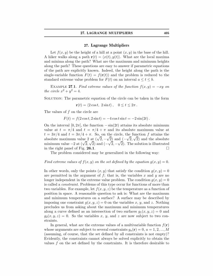
27. LAGRANGE MULTIPLIERS 405
27. Lagrange Multipliers
Let f(x, y) be the height of a hill at a point (x, y) in the base of the hill.A hiker walks along a path r(t) = 〈x(t), y(t)〉. What are the local maximaand minima along the path? What are the maximum and minimum heightsalong the path? These questions are easy to answer if parametric equationsof the path are explicitly known. Indeed, the height along the path is thesingle-variable function F (t) = f(r(t)) and the problem is reduced to thestandard extreme value problem for F (t) on an interval a ≤ t ≤ b.
Example 27.1. Find extreme values of the function f(x, y) = −xy onthe circle x2 + y2 = 4.
Solution: The parametric equation of the circle can be taken in the form
r(t) = 〈2 cos t, 2 sin t〉 , 0 ≤ t ≤ 2π .
The values of f on the circle are
F (t) = f(2 cos t, 2 sin t) = −4 cos t sin t = −2 sin(2t) .
On the interval [0, 2π], the function − sin(2t) attains its absolute minimumvalue at t = π/4 and t = π/4 + π and its absolute maximum value att = 3π/4 and t = 3π/4 + π. So, on the circle, the function f attains theabsolute maximum value 2 at (
√2,−
√2) and (−
√2,√
2) and the absolute
minimum value −2 at (√
2,√
2) and (−√
2,−√
2). The solution is illustratedin the right panel of Fig. 26.1. �
The problem considered may be generalized in the following way:
Find extreme values of f(x, y) on the set defined by the equation g(x, y) = 0.
In other words, only the points (x, y) that satisfy the condition g(x, y) = 0are permitted in the argument of f ; that is, the variables x and y are nolonger independent in the extreme value problem. The condition g(x, y) = 0is called a constraint. Problems of this type occur for functions of more thantwo variables. For example, let f(x, y, z) be the temperature as a function ofposition in space. A reasonable question to ask is: What are the maximumand minimum temperatures on a surface? A surface may be described byimposing one constraint g(x, y, z) = 0 on the variables x, y, and z. Nothingprecludes us from asking about the maximum and minimum temperaturesalong a curve defined as an intersection of two surfaces g1(x, y, z) = 0 andg2(x, y, z) = 0. So the variables x, y, and z are now subject to two con-straints.
In general, what are the extreme values of a multivariable function f(r)whose arguments are subject to several constraints ga(r) = 0, a = 1, 2, ...,M(assuming, of course, that the set defined by all constraints is not empty)?Evidently, the constraints cannot always be solved explicitly to obtain thevalues f on the set defined by the constraints. It is therefore desirable to
406 3. DIFFERENTIATION OF MULTIVARIABLE FUNCTIONS
develop a technique to find extreme values of f without solving the con-straints. If constraints are level sets of differentiable functions, then thistechnique is known the method of Lagrange multipliers.
Definition 27.1. (Local Maxima and Minima Subject to Constraints).A function f has a local maximum (or minimum) at r0 on the set definedby constraints ga(r) = 0, a = 1, 2, ...,M , if f(r) ≤ f(r0) (or f(r) ≥ f(r0))for all r in some neighborhood of r0 that satisfy the constraints, that is,ga(r) = 0.
The extreme values of a function subject to constraints are defined sim-ilarly.
Definition 27.2. (Extreme Values of a Function Subject to Constraints)A function f has a maximum (or minimum) value at a point r0 on theset defined by constraints ga(r) = 0, a = 1, 2, ...,M , if f(r) ≤ f(r0) (orf(r) ≥ f(r0)) for all r such that ga(r) = 0.
Note that a function f may not have local maxima or minima in itsdomain. However, when its arguments become subject to constraints, it maywell have local maxima and minima on the set defined by the constraints.In the example considered, f(x, y) = −xy has no local maxima or minima,but, when it is restricted on the circle by imposing the constraint g(x, y) =x2 + y2 − 4 = 0, it happens to have two local minima and maxima. In thiscase, the local maxima and minima also determine the extreme values of thefunction f on the circle.
27.1. Critical Points of a Function Subject to a Constraint. The extremevalue problem with constraints amounts to finding the critical points ofa function whose arguments are subject to constraints. Suppose that fis a differentiable function. The example discussed above shows that theequation ∇f = 0 no longer determines the critical points of f in the setdefined by constraints. A new condition has to be found.
Consider first the case of a single constraint for two variables r = 〈x, y〉.Let r0 be a point at which a differentiable function f has a local extremumon the set S defined by the constraint g(r) = 0. Let us further assume that ghas continuous partial derivatives in a neighborhood of r0 and ∇g(r0) 6= 0.Then by the analysis of Section 24.2 the equation g(r) = 0 defines a smoothcurve through the point r0. Let r(t) be parametric equations of this curvein a neighborhood of r0, that is, for some t = t0, r(t0) = r0 and r′(t0) 6= 0(a smooth curve has a tangent vector at any point). The function F (t) =f(r(t)) defines values of f along the curve and has a local extremum at t0.Since the curve is smooth, the vector function r(t) is differentiable and itis concluded that F has no rate of change at t = t0, F ′(t0) = 0. Since f isa differentiable function, the derivative F ′(t0) can also be computed by the
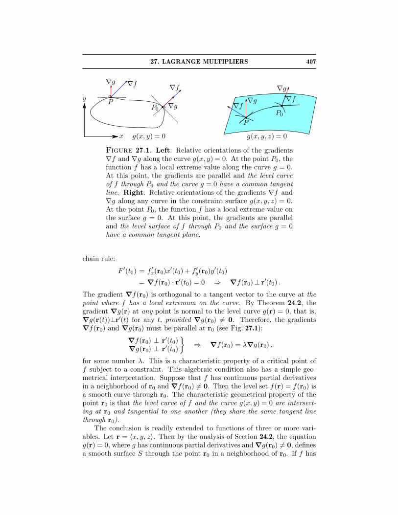
27. LAGRANGE MULTIPLIERS 407
∇g ∇f
PP0
∇f
∇gy
x g(x, y) = 0
∇f∇g
P
∇g
∇f
P0
g(x, y, z) = 0
Figure 27.1. Left: Relative orientations of the gradients∇f and ∇g along the curve g(x, y) = 0. At the point P0, thefunction f has a local extreme value along the curve g = 0.At this point, the gradients are parallel and the level curveof f through P0 and the curve g = 0 have a common tangentline. Right: Relative orientations of the gradients ∇f and∇g along any curve in the constraint surface g(x, y, z) = 0.At the point P0, the function f has a local extreme value onthe surface g = 0. At this point, the gradients are paralleland the level surface of f through P0 and the surface g = 0have a common tangent plane.
chain rule:
F ′(t0) = f ′x(r0)x
′(t0) + f ′y(r0)y
′(t0)
= ∇f(r0) · r′(t0) = 0 ⇒ ∇f(r0)⊥ r′(t0) .
The gradient ∇f(r0) is orthogonal to a tangent vector to the curve at thepoint where f has a local extremum on the curve. By Theorem 24.2, thegradient ∇g(r) at any point is normal to the level curve g(r) = 0, that is,∇g(r(t))⊥r′(t) for any t, provided ∇g(r0) 6= 0. Therefore, the gradients∇f(r0) and ∇g(r0) must be parallel at r0 (see Fig. 27.1):
∇f(r0) ⊥ r′(t0)∇g(r0) ⊥ r′(t0)
}
⇒ ∇f(r0) = λ∇g(r0) ,
for some number λ. This is a characteristic property of a critical point off subject to a constraint. This algebraic condition also has a simple geo-metrical interpretation. Suppose that f has continuous partial derivativesin a neighborhood of r0 and ∇f(r0) 6= 0. Then the level set f(r) = f(r0) isa smooth curve through r0. The characteristic geometrical property of thepoint r0 is that the level curve of f and the curve g(x, y) = 0 are intersect-ing at r0 and tangential to one another (they share the same tangent linethrough r0).
The conclusion is readily extended to functions of three or more vari-ables. Let r = 〈x, y, z〉. Then by the analysis of Section 24.2, the equationg(r) = 0, where g has continuous partial derivatives and ∇g(r0) 6= 0, definesa smooth surface S through the point r0 in a neighborhood of r0. If f has
408 3. DIFFERENTIATION OF MULTIVARIABLE FUNCTIONS
a local extreme value at r0 on the surface g(r) = 0, then f attains a localextreme value along any smooth curve r = r(t) through r0 in that surface.Therefore the derivative
F ′(t) =d
dtf(r(t)) = f ′
xx′ + f ′yy
′ + f ′zz
′ = ∇f(r(t)) · r′(t)
must vanish at t0 for which r(t0) = r0. Therefore, the gradient ∇f(r0) isorthogonal to a tangent vector of any smooth curve in the surface S at r0:
F ′(t0) = ∇f(r0) · r′(t0) = 0 ⇒ ∇f(r0) ⊥ r′(t0) .
On the other hand, by the properties of the gradient (Theorem 24.2), thevector ∇g(r0) is orthogonal to r′(t0) for every such curve. Therefore, at thepoint r0, the gradients of f and g are orthogonal to the tangent plane of Sand, hence, must be parallel. A similar line of reasoning proves the followingtheorem for any number of variables.
Theorem 27.1. (Critical Points Subject to a Constraint).Suppose that f has a local extreme value at a point r0 on the set defined bya constraint g(r) = 0. Suppose that g has continuous partial derivatives ina neighborhood of r0 and ∇g(r0) 6= 0. If f is differentiable at r0, then thereexists a number λ such that
∇f(r0) = λ∇g(r0).
This theorem provides a powerful method to find critical points of fsubject to a constraint g = 0. It is called the method of Lagrange multipliers.To find the critical points of f , the following system of equations must besolved:
(27.1) ∇f(r) = λ∇g(r) , g(r) = 0.
If r = 〈x, y〉, this is a system of three equations:
f ′x(x, y) = λg′x(x, y)
f ′y(x, y) = λg′y(x, y)
g(x, y) = 0
for three variables (x, y, λ). For each solution (x0, y0, λ0), the correspondingcritical point of f is (x0, y0). The numerical value of λ is not relevant;only its existence must be established by solving the system. In the caseof functions of three variables, the system contains four equations for fourvariables (x, y, z, λ):
f ′x(x, y, z) = λg′x(x, y, z)
f ′y(x, y, z) = λg′y(x, y, z)
f ′z(x, y, z) = λg′z(x, y, z)
g(x, y, z) = 0
For each solution (x0, y0, z0, λ0), the corresponding critical point of f is(x0, y0, z0).
27. LAGRANGE MULTIPLIERS 409
On applicability of the Lagrange method. Suppose that f has a local ex-tremum at a point r0 on a curve g(r) = 0. The hypothesis ∇g(r0) 6= 0 inTheorem 27.1 is crucial for the method of Lagrange multipliers to work. If∇f(r0) 6= 0 (i.e. r0 is not a critical point of f without the constraint), thenEqs. (27.1) have no solution when ∇g(r0) = 0, and the method of Lagrangemultiplers fails to detect a local extremum of f . Recall that the derivationof Eq. (27.1) requires that a curve defined by the equation g(r) = 0 issmooth near r0, which may no longer be the case if ∇g(r0) = 0. So, if fattains its local extreme value at a point where the curve g(x, y) = 0 is notsmooth, then this point cannot be determined by Eq. (27.1). For example,the equation
g(x, y) = x3 − y2 = 0 ⇒ x = y2/3
defines a curve that has a cusp at (0, 0) and ∇g(0, 0) = 0. Since x = y2/3 ≥ 0on the curve, the function
f(x, y) = x ⇒ f(y2/3, y) = y2/3 , −∞ < y < ∞ ,
attains its absolute minimum value 0 along this curve at the origin. However,∇f(0, 0) = 〈1, 0〉 6= 0 and the method of Lagrange multipliers fails to detectthis point because there is no λ at which Eqs. (27.1) are satisfied.
On the other hand, the function f(x, y) = x2 also attains its abso-lute minimum value at the origin. Equations (27.1) do have the solution(x, y, λ) = (0, 0, 0). The difference between the two cases is that in the lat-ter case ∇f(0, 0) = 0, i.e., (0, 0) is also a critical point of f without theconstraint. Thus, if the gradient ∇g vanishes at some points in the set de-fined by the constraint g = 0, then these points should also be studied ascritical points of a function f subject to the constraint g = 0.
27.2. Extreme Value Problem Subject to a Constraint. A differentiablefunction does not necessarily attains its extreme values on a set defined bya constraint g = 0. For example, f(x, y) = xy has no maximum value ofthe line g(x, y) = y − x = 0, but it attains its minimum value because thevalues of f on the line are f(x, x) = x2 where x is any real. On the lineg(x, y) = y + x = 0, the function f has no minimum value, but attains itsmaximum value: f(x,−x) = −x2. On the parabola g(x, y) = y − x2 = 0,the function f has no maximum and minimum values because f(x, x2) = x3.So, the mere existence of critical points as solutions to Eqs. (27.1) does notguarantee that f has extreme values at a critical point.
If, however, a differentiable function f is known to attain its extremevalues on a set defined by a constraint g = 0 where g is also a differentiablefunction, then finding the extreme values becomes a two-steps procedure:
Step 1. Find all solutions (r, λ) = (r0, λ0) of the system (27.1); find allpoints in the set g = 0 where ∇g = 0.
410 3. DIFFERENTIATION OF MULTIVARIABLE FUNCTIONS
Step 2. Evaluate f at all the critical points that result from Step 1. Thelargest of these values is the maximum value of f ; the smallest isthe minimum value of f .
The extreme value theorem (Theorem 26.2) provides sufficient condi-tions under which the above two-steps procedure allows us to find the ex-treme values of a function subject to constraints. If the constraints definea closed and bounded set, then a differentiable function attains its extremevalues on the set at some of the critical points determined by the method ofLagrange multipliers.
If g(x, y) = 0 define a piecewise smooth curve that is a boundary of abounded region in a plane, then that curve is a closed bounded set. A linein a plane is a closed, but not bounded set because it is not contained inany disk. Similarly, if g(x, y, z) = 0 define a piecewise smooth surface thatis a boundary of a bounded region in space, then that surface is a closedbounded set. A plane or a line in space is not a bounded set as these setsare not contained in any ball.
Example 27.2. Use the method of Lagrange multipliers to solve the theproblem in Example 27.1.
Solution: Put g(x, y) = x2 + y2 − 4. The functions f(x, y) = −xy and gare differentiable everywhere as they are polynomials.Step 1: Then
f ′x = λg′x
f ′y = λg′y
g = 0⇒
−y = 2λx−x = 2λy
x2 + y2 = 4.
The substitution of the first equation into the second one gives x = 4λ2x.This means that either x = 0 or λ = ±1/2. If x = 0, then y = 0 by the firstequation, which contradicts the constraint. For λ = 1/2, x = −y and theconstraint gives 2x2 = 4 or x = ±
√2. The critical points corresponding to
λ = 1/2 are
P1 = (√
2,−√
2) , P2 = (−√
2,√
2) .
If λ = −1/2, x = y and the constraint gives 2x2 = 4 or x = ±√
2. Thecritical points corresponding to λ = −1/2 are
P3 = (√
2,√
2) , P4 = (−√
2,−√
2) .
The gradient ∇g(x, y) = 〈2x, 2y〉 vanishes only at the origin which is not onthe circle x2 + y2 = 4. Alternatively, one could just notice that a circle is asmooth curve.Step 2: The circle x2 + y2 = 4 is is a closed, bounded set in the planeas a boundary of a disk. So f attains its extreme values at (some of)the found critical points: f(±
√2,∓
√2) = 2 is the maximum value and
f(±√
2,±√
2) = −2 is the minimum one. �
27. LAGRANGE MULTIPLIERS 411
27.3. The Nature of Critical Points Subject to a Constraint. The mereexistence of a solution to (27.1) does not guarantee that f has a local ex-tremum at the point found. The situation is fully analogous to finding localextrema of a differentiable function without constraints: the function inquestion does not necessarily attains a local extremum value at each criticalpoint. An additional study is needed to determine the nature of a criticalpoint (e.g., the second derivative test). For example, in the case of a func-tion f of two variables subject to a constraint g = 0, Eq. (27.1) means thatthe function f has no rate of change along the curve g = 0 at a particularpoint of the curve. This can happen not only when f has a local extremumat this point, but also when f has an inflection point along the curve. Hereis an example of this kind.
Consider the following function and constraint
f(x, y) = xy , g(x, y) = y − x2 = 0 .
It is easy to see that the constraint defines the parabola y = x2 in the plane.The function f has no extreme values on the parabola: f(x, x2) = x3 where−∞ < x < ∞. However, the system (27.1) has one solution:
f ′x = λg′x
f ′y = λg′yg = 0
⇒
y = −2λxx = λy = x2
⇒ (x, y, λ) = (0, 0, 0) .
The substitution of the first and second equations into the third one yields−2λ2 = λ2 or λ = 0, and, hence, x = y = 0. Note that f(x, x2) = x3 has aninflection point at x = y = 0.
How does one determine the nature of a critical point in the case ofconstrains? There is an analog of the second derivative test in the case ofa constrained extreme value problem. It will be discussed in Section 27.6.However, this test is generally far more difficult to use than the secondderivative test for non-constrained extreme value problems. So, a direct useof Definition 27.1 often works better. Yet, in the case when constraintsdefine a curve, there is a simple way to determine the nature of criticalpoints.
Let g(x, y) = 0 define a smooth curve so that all critical points P1, P2,..., Pn are solutions to (27.1). Suppose that it is known that f has a localmaximum at P1 on the curve. For instance, if the curve is closed, then bythe extreme value theorem f attains its maximum value at one of the criticalpoints, say, P1. In particular, it is also a local maximum. The critical pointscan always be ordered along the curve, that is, if a curve is traversed in aparticular direction, then the point Pk follows the point Pk−1, k = 2, 3, ....Since f has a local maximum at P1, it should have either a local minimum oran inflection at the neighboring critical point P2 along the curve. Let P3 bethe critical point next to P2 along the curve. Then f has a local minimumat P2 if f(P2) < f(P3) and an inflection if f(P2) > f(P3). In other words,
412 3. DIFFERENTIATION OF MULTIVARIABLE FUNCTIONS
• Only a local minimum (maximum) can occur at the only criticalpoint between two neighboring local maxima (minima);
• One or more consecutive inflection points can only occur betweentwo neighboring local maximum and minimum.
This procedure may be continued until all critical points are exhausted.Compare this pattern of critical points with the behavior of a height alonga hiking path.
Example 27.3. Find all critical points of the function f(x, y) = x2y onthe circle x2 + y2 = 1 and determine the nature of each critical point.
Solution: The function f is a polynomial and hence differentiable every-where. The constraint g(x, y) = x2 +y2−1 = 0 is defined by a differentiablefunction g(x, y) whose gradient ∇g = 〈2x, 2y〉 does not vanish anywhere onthe circle. Therefore all critical point of f are determined by solutions ofthe system (27.1):
f ′x = λg′x
f ′y = λg′yg = 0
⇒
2xy = 2λxx2 = 2λy
x2 + y2 = 1
It follow from the first equation that either x = 0 or y = λ. If x = 0, theny = ±1 (by the constraint) and λ = 0 (by the second equation). So, (0,±1)are critical points corresponding to λ = 0. If y = λ, then by the secondequation x2 = 2λ2. Then by the constraint x2 + y2 = 3λ2 = 1 and, hence,λ = ±1/
√3. Thus, (±
√
(2/3), 1/√
3) are critical points corresponding to
λ = 1/√
3 and (±√
(2/3),−1/√
3) are critical points corresponding to λ =
−1/√
3. Let us order the critical points along the circle counterclockwisestarting from the point in the positive quadrant:
P1 = (√
(2/3), 1/√
3) , P2 = (0, 1) , P3 = (−√
(2/3), 1/√
3) ,
P4 = (−√
2/3,−1/√
3) , P5 = (0,−1) , P6 = (√
(2/3),−1/√
3) .
By examining the sequence of values of f at the critical points
f(P1) → f(P2) → f(P3) → f(P4) → f(P5) → f(P6)√2
3√
3→ 0 →
√2
3√
3→ −
√2
3√
3→ 0 → −
√2
3√
3
max → min → max → min → max → min
it is concluded that the function f has local maxima at P1, P3 and P5 andit has local minima at P2, P4, and P6. �
27.4. Applications of the method of Lagrange multipliers. The method ofLagrange multipliers is used in various optimization problems where someof the variables are not independent and subject to constraints.
Example 27.4. A rectangular box without a lid is to be made from card-board. Find the dimensions of the box of a given volume V such that thecost of material is minimal.
27. LAGRANGE MULTIPLIERS 413
Solution: Let the dimensions of the box be x, y, and z, where z is theheight. The amount of cardboard needed is determined by the surface area
f(x, y, z) = xy + 2xz + 2yz .
The question is to find the minimal value of f subject to constraint that thevolume of the box has a given value V :
g(x, y, z) = xyz − V = 0 .
Since f and g have continuous partial derivatives, let us apply the methodof Lagrange multipliers:
f ′x = λg′x
f ′y = λg′y
f ′z = λg′z
g = 0
⇒
y + 2z = λyzx + 2z = λxz
2x + 2y = λxyxyz = V
⇒
xy + 2xz = λVxy + 2zy = λV
2xz + 2yz = λVxyz = V
,
where the last system has been obtained by multiplying the first equationby x, the second one by y, and the third one by z with the subsequent use ofthe constraint. Combining the first two equations, one infers 2z(y − x) = 0.Since z 6= 0 (V 6= 0), one has y = x. Combining the first and third equations,one infers y(x− 2z) = 0 and hence x = 2z. The substitution of y = x = 2zinto the constraint yields 4z3 = V . Hence, the optimal dimensions are
x = y = (2V )1/3 , z =1
2(2V )1/3 .
The amount of cardboard minimizing the cost is 3(2V )2/3 (the value of fat the critical point). From the geometry of the problem, it is clear that fattains its minimum value at the only critical point. �
Extreme values on a set. The method of Lagrange multipliers can be usedto determine extreme values of a function on a set D. Recall that theextreme values may occur on the boundary of D. In Example 26.3, explicitparametric equations of the boundary of D have been used (Step 2 in thesolution). Instead, an algebraic equation of the boundary,
g(x, y) = x2 + y2 − 4 = 0
can be used in combination with the method of Lagrange multipliers. In-deed, if
f(x, y) = x2 + y2 + xy ,
then its critical points along the boundary circle satisfy the system of equa-tions:
f ′x = λg′x
f ′y = λg′y
g = 0=⇒
2x + y = 2λx2y + x = 2λy
x2 + y2 = 4.
By subtracting the second equation from the first one, it follows that
x − y = 2λ(x− y) .
414 3. DIFFERENTIATION OF MULTIVARIABLE FUNCTIONS
Hence, either x = y or λ = 1/2. In the former case, the constraint yields
2x2 = 4 or x = ±√
2. The corresponding critical points are (±√
2,±√
2).If λ = 1/2, then from the first two equations in the system, one infers that
x = −y. The constraint becomes 2x2 = 4 or x = ±√
2, and the criticalpoints are (±
√2,∓
√2).
27.5. The Case of Two or More Constraints. Let a differentiable functionof three variables f have a local extreme value at point r0 on the set definedby two constraints g1(r) = 0 and g2(r) = 0. Suppose that g1 and g2 havecontinuous partial derivatives in a neighborhood of r0 and the gradients ofg1 and g2 do not vanish at r0, ∇g1(r0) 6= 0 and ∇g2(r0) 6= 0. Then eachconstraint defines a smooth surface in a neighborhood of r0. Suppose thatthe vectors ∇g1(r0) and ∇g2(r0) are not parallel or, equivalently, ∇g1(r0)is not proportional to ∇g2(r0). Then the set defined by the constraints is asmooth curve of intersection of two surfaces. Let v be a tangent vector tothe curve at r0. Since the curve lies in the level surface g1 = 0, by the earlierarguments, ∇f(r0)⊥v and ∇g1(r0)⊥v. On the other hand, the curve alsolies in the level surface g2 = 0 and hence ∇g2(r0)⊥v. It follows that thegradients ∇f , ∇g1, and ∇g2 become coplanar at the point r0 as they liein the plane normal to v. Any vector in the plane normal to v is a linearcombination of two non-parallel vectors in it. Therefore there exist numbersλ1 and λ2 such that
∇f(r) = λ1∇g1(r) + λ2∇g2(r) , g1(r) = g2(r) = 0
when r = r0. This is a system of five equations for five variables (x, y, z, λ1, λ2).For any solution (x0, y0, z0, λ10, λ20), the point (x0, y0, z0) is a critical pointof f on the set defined by the constraints. In general, the following resultcan be proved by a similar line of reasoning.
Theorem 27.2. (Critical Points Subject to Constraints).Suppose that functions ga, a = 1, 2, ..., M , of m variables, m > M , havecontinuous partial derivatives in a neighborhood of a point r0 and a func-tion f has a local extreme value at r0 in the set defined by the constraintsga(r) = 0. Suppose that ∇ga(r0) are non-zero vectors any of which cannotbe expressed as a linear combination of the others and f is differentiable atr0. Then there exist numbers λa such that
∇f(r0) = λ1∇g1(r0) + λ2∇g2(r0) + · · ·+ λM∇gM(r0).
Example 27.5. Find extreme values of the functions f(x, y, z) = xyzon the curve that is an intersection of the sphere x2 + y2 + z2 = 1 and theplane x + y + z = 0.
Solution: Put g1(x, y, z) = x2 + y2 + z2 − 1 and g2(x, y, z) = x + y + z.One has ∇g1 = 〈2x, 2y, 2z〉 which can only vanish at (0, 0, 0) and, hence,∇g1 6= 0 on the sphere. Also, ∇g2 = 〈1, 1, 1〉 6= 0. Therefore critical points
27. LAGRANGE MULTIPLIERS 415
of f on the surface of constraints are determined by the equations:
f ′x = λ1g
′x + λ2g
′x
f ′y = λ1g
′y + λ2g
′y
f ′z = λ1g
′z + λ2g
′z
g1 = 0g2 = 0
⇒
yz = 2λ1x + λ2
xz = 2λ1y + λ2
xy = 2λ1z + λ2
1 = x2 + y2 + z2
0 = x + y + z
Subtract the second equation from the first one to obtain that (y − x)z =2λ1(x−y). It follows then that either x = y or z = −2λ1. Suppose first thaty = x. Then z = −2x by the fifth equation. The substitution of x = y andz = −2x into the fourth equation yields 6x2 = 1 or x = ±1/
√6. Therefore
the points
r1 = 〈1/√
6, 1/√
6,−2/√
6〉 , r2 = 〈−1/√
6,−1/√
6, 2/√
6〉
are critical points, provided there exist the corresponding values λ1 and λ2
such that all equations are satisfied. For example, take r1. Then the secondand third equations become
{
−26 = 2√
6λ1 + λ2
16 = − 4√
6λ1 + λ2
⇔{
−36 = 6√
6λ1
16 = − 4√
6λ1 + λ2
So λ1 = −1/(2√
6) and λ2 = −1/6. The existence of λ1 and λ2 for thepoint r2 is verified similarly. Next suppose that z = −2λ1. Subtract thethird equation from the second one to obtain that (z − y)x = 2λ1(y − z). Itfollows that either y = z or x = −2λ1. Let y = z. The fifth equation yieldsx = −2y and the fourth equation is reduced to 6y2 = 1. Therefore there aretwo more critical points
r3 = 〈−2/√
6, 1/√
6, 1/√
6〉 , r4 = 〈2/√
6,−1/√
6,−1/√
6〉 .
The reader is to verify the existence of λ1 and λ2 in these cases (note thatλ1 = −z/2). Finally, let x = −2λ1 and z = −2λ1. These conditions implythat x = z and, by the fifth equation, y = −2x. The fourth equation yields6x2 = 1 so that there is another pair of critical points:
r5 = 〈1/√
6,−2/√
6, 1/√
6〉 , r6 = 〈−1/√
6, 2/√
6,−1/√
6〉
(the reader is to verify the existence of λ1 and λ2). The intersection of thesphere and the plane is a circle, which is a closed and bounded set. So, fattains its extreme values at some of the critical points found. By examiningthe largest and smallest values of f at the critical points, it is concluded thatf attains the maximum value 2/
√6 at r2, r4, and r6 and the minimum value
−2/√
6 at r1, r3, and r5. �
Let f(r) be a function subject to a constraint g(r). Define the function
F (r, λ) = f(r) − λg(r),
416 3. DIFFERENTIATION OF MULTIVARIABLE FUNCTIONS
where λ is viewed as an additional independent variable. Then critical pointsof F are determined by (27.1). Indeed, if r = 〈x1, x2, ..., xm〉, then
F ′λ(r, λ) = 0 ⇒ g(r) = 0
F ′xj
(r, λ) = 0 ⇒ f ′xj
(r, λ)− λg′xj(r, λ) = 0 ⇒ ∇f = λ∇g .
Similarly, if there are several constraints, critical points of the function withadditional variables λa, a = 1, 2, ..., M ,
(27.2) F (r, λ1, λ2, ..., λM) = f(r)−M∑
a=1
λaga(r)
coincide with the critical points of f subject to the constraints ga = 0 asstated in Theorem 27.2. The functions F and f have the same values onthe set defined by the constraints ga = 0 because they differ by a linearcombination of constraint functions with the coefficients being the Lagrangemultipliers. The above observation provides a simple way to formulate theequations for critical points subject to constraints.
27.6. Finding Local Maxima and Minima. In the simplest case of a func-tion f of two variables subject to a constraint, the nature of critical pointshas been determined by ordering critical points along the curve and by ex-amining the values of the function at the critical points. Unfortunately, thismethod is limited in applications. For example, if the constraint definesa surface, then it is not possible to order critical points. It is possible todevelop an analog of the second-derivative test for critical points subject toconstraints.
The second-derivative test. If the constraints can be solved, then an ex-plicit form of f on the set defined by the constraints can be found, and thestandard second-derivative test applies! For instance, in Example 27.4, theconstraint can be solved z = V/(xy). The values of the function f on theconstraint surface are
F (x, y) = f(x, y, V/(xy)) = xy +2V (x + y)
xy.
The equations F ′x = 0 and F ′
y = 0 determine the critical point x = y =
(2V )1/3 (and z = V/(xy) = (2V )1/3/2). So the second-derivative test can
be applied to the function F (x, y) at the critical point x = y = (2V )1/3 toshow that indeed F has a minimum and hence f has a minimum on theconstraint surface.
Even if the constraint cannot be solved explicitly, the implicit functiontheorem may be used to obtain an analog of the second-derivative test forcritical points of functions subject to constraints. Its general formulation isnot simple. So the discussion is limited to the simplest case of a functionof two variables subject to a constraint (see also Study Problem 27.2 wherethe case of three variables and one constraint is studied).

27. LAGRANGE MULTIPLIERS 417
Suppose that g and f have continuous second order partial derivativesand ∇g(r0) 6= 0 where r0 is a solution of the system (27.1) for some λ. Theng′x and g′y cannot simultaneously vanish at the critical point. Without loss
of generality, assume that g′y 6= 0 at r0. By the implicit function theorem,there is a neighborhood of r0 in which the equation g(x, y) = 0 has a uniquesolution y = h(x). The values of f on the level curve g = 0 near the criticalpoint are F (x) = f(x, h(x)). By the chain rule, one infers that F ′ = f ′
x+f ′yh
′
and
(27.3) F ′′ = (d/dx)(f ′x + f ′
yh′) = f ′′
xx + 2f ′′xyh
′ + f ′′yy(h′)2 + f ′
yh′′.
So, in order to find F ′′(x0), one has to calculate h′(x0) and h′′(x0). Thislatter task is accomplished by the implicit differentiation.
By the definition of h(x), G(x) = g(x, h(x)) = 0 for all x in an openinterval containing x0. Therefore, G′(x) = 0, which defines h′:
G(x) = 0 ⇒ 0 = G′(x) = g′x(x, h) + g′y(x, h)h′(x) ⇒ h′(x) = −g′xg′y
.
Similarly, G′′(x) = 0 yields
(27.4) G′′ = g′′xx + 2g′′xyh′ + g′′yy(h
′)2 + g′yh′′ = 0,
which can be solved for h′′:
h′′ = − 1
g′y
(
g′′xx + 2g′′xyh′ + g′′yy(h
′)2)
, h′ = −g′xg′y
So the derivatives h′(x0) and h′′(x0) can be computed in terms of the valuesof the partial derivatives of g at the critical point (x0, y0). Their substitutioninto (27.3) gives the value F ′′(x0). If F ′′(x0) > 0 (or F ′′(x0) < 0), then f hasa local minimum (or maximum) at (x0, y0) along the curve g = 0. Note alsothat F ′(x0) = 0 as required owing to the conditions f ′
x = λg′x and f ′y = λg′y
satisfied at the critical point.If g′y(r0) = 0, then g′x(r0) 6= 0, and there is a function x = h(y) that
solves the equation g(x, y) = 0. So, by swapping x and y in the abovearguments, the same conclusion is proved to hold.
Example 27.6. Show that the point r0 = 0 is a critical point of thefunction f(x, y) = x2y + y + x subject to the constraint exy = x + y + 1 anddetermine whether f has a local minimum or maximum at it.
Solution:
Critical point. Put g(x, y) = exy − x − y − 1. Then g(0, 0) = 0; that is, thepoint (0, 0) satisfies the constraint. The first partial derivatives of f and gare
f ′x = 2xy + 1 , f ′
y = x2 + 1 , g′x = yexy − 1 , g′y = xexy − 1 .
Therefore, both equations f ′x(0, 0) = λg′x(0, 0) and f ′
y(0, 0) = λg′y(0, 0) aresatisfied at λ = −1. Thus, the point (0, 0) is a critical point of f subject to

418 3. DIFFERENTIATION OF MULTIVARIABLE FUNCTIONS
the constraint g = 0.Second-derivative test. Since g′y(0, 0) = −1 6= 0, there is a function y = h(x)near x = 0 such that G(x) = g(x, h(x)) = 0. By the implicit differentiation,
h′(0) = −g′x(0, 0)/g′y(0, 0) = −1 .
The second partial derivatives of g are
g′′xx = y2exy , g′′yy = x2exy , g′′xy = exy + xyexy .
The derivative h′′(0) is found from (27.4), where g′′xx(0, 0) = g′′yy(0, 0) = 0,
g′′xy(0, 0) = 1, h′(0) = −1, and g′y(0, 0) = −1:
h′′(0) = −[g′′xx(0, 0) + 2g′′xy(0, 0)h′(0) + g′′yy(0, 0)(h′(0))2]/g′y(0, 0) = −2.
The second partial derivatives of f are
f ′′xx = 2y , f ′′
yy = 0 , f ′′xy = 2x.
The substitution of f ′′xx(0, 0) = f ′′
yy(0, 0) = f ′′xy(0, 0) = 0, h′(0) = −1,
f ′y(0, 0) = 1, and h′′(0) = −2 into (27.3) gives F ′′(0) = −2 < 0. There-
fore, f attains a local maximum at (0, 0) along the curve g = 0. Note alsothat F ′(0) = f ′
x(0, 0) + f ′y(0, 0)h′(0) = 1 − 1 = 0 as required. �
The implicit differentiation and the implicit function theorem can beused to establish the second-derivative test for the multivariable case withconstraints (see another example in Study Problem 27.2).
27.7. Study Problems.
Problem 27.1. An axially symmetric solid consists of a circular cylinderand a right-angled circular cone attached to one of the cylinder’s bases. Whatare the dimensions of the solid at which it has a maximal volume if thesurface area of the solid has a fixed value S?
Solution: Let r and h be the radius and height of the cylinder. Since thecone is right-angled, its height is r. The surface area is the sum of threeterms: the area of the base (disk) πr2, the area of the side of the cylinder2πrh, and the surface area Sc of the cone. A cone of height a and withthe radius of the base r is obtained by rotation of a straight line y = mx,where m = r/a and 0 ≤ x ≤ a, about the x−axis. In the present case r = aand m = 1. Recall from Calculus II that the area of a surface obtained byrotation about the x axis is
Sc =
∫ a
02πy
√
1 + (dy/dx)2dx =√
2
∫ r
02πxdx = π
√2 r2 .
Similarly, the volume of the cone is
Vc =
∫ a
0πy2dx =
∫ r
0πx2dx =
πr3
3.

27. LAGRANGE MULTIPLIERS 419
Therefore the problem is reduced to finding the maximal value of the func-tion (volume) V (r, h) = πr2h + πr3/3 subject to the constraint
g(r, h) = 2πrh + (1 +√
2)πr2 − S = 0 .
The critical points of V satisfy the equations:
V ′r = λg′r
V ′h = λg′h0 = g(r, h)
⇒
2πrh + πr2h = λ(2πh + 2(1 +√
2)πr)πr2 = 2πλr
S = 2πrh + (1 +√
2)πr2
Since r 6= 0 (the third equation is not satisfied if r = 0), the second equationimplies that λ = r/2. The substitution of the latter into the first equation
yields rh = r2√
2 or h = r√
2. Then it follows from the third equation thatr = (S/[π(1 + 2
√2)])1/2. By the geometrical nature of the problem it is
clear that the found critical point corresponds to the maximum value of thevolume. �
Problem 27.2. Let functions f and g of three variables r = 〈x, y, z〉 havecontinuous partial derivatives up to order 2. Use the implicit differentiationto establish the second-derivative test for critical points of f on the surfaceg(r) = 0.
Solution: Suppose that ∇g(r0) 6= 0 at a critical point r0. Withoutloss of generality, one can assume that g′z(r0) 6= 0. By the implicit func-tion theorem, there exists a function z = h(x, y) such that G(x, y) =g(x, y, h(x, y)) = 0 in some neighborhood of the critical point. Then theequations G′
x(x, y) = 0 and G′y(x, y) = 0 determine the first partial deriva-
tives of h:
g′x + g′zh′x = 0 ⇒ h′
x = −g′x/g′z ; g′y + g′zh′y = 0 ⇒ h′
y = −g′y/g′z .
The second partial derivatives h′′xx, h′′
xy, and h′′yy are found from the equations
G′′xx = 0 ⇒ g′′xx + 2g′′xzh
′x + g′′zz(h
′x)
2 + g′zh′′xx = 0,
G′′yy = 0 ⇒ g′′yy + 2g′′yzh
′y + g′′zz(h
′y)
2 + g′zh′′yy = 0,
G′′xy = 0 ⇒ g′′xy + g′′xzh
′x + g′′yzh
′y + g′′zzh
′xh′
y + g′zh′′xy = 0.
The values of the function f on the level surface g(x, y, z) = 0 near thecritical point are F (x, y) = f(x, y, h(x, y)). To apply the second-derivativetest to the function F , its second partial derivatives have to be computedat the critical point. By the chain rule
F ′′xx = (f ′
x + f ′zh
′x)′x = f ′′
xx + 2f ′′xzh
′x + f ′′
zz(h′x)
2 + f ′zh
′′xx,
F ′′yy = (f ′
y + f ′zh
′y)
′y = f ′′
yy + 2f ′′yzh
′y + f ′′
zz(h′y)
2 + f ′zh
′′yy,
F ′′xy = (f ′
x + f ′zh
′x)′y = f ′′
xy + f ′′xzh
′x + f ′′
yzh′y + f ′′
zzh′xh′
y + f ′zh
′′xy,
where the first and second partial derivatives of h have been found earlier.If (x0, y0, z0) is the critical point found by solving the system (27.1), then
420 3. DIFFERENTIATION OF MULTIVARIABLE FUNCTIONS
a = F ′′xx(x0, y0), b = F ′′
yy(x0, y0), and c = F ′′xy(x0, y0) in the second-derivative
test for the two-variable function F . �
27.8. Exercises.1–18. Use Lagrange multipliers to find the maximum and minimum valuesof each of the following functions subject to the specified constraints:
1. f(x, y) = xy, x + y = 1 ;2. f(x, y) = x2 + y2, x/a + y/b = 1 ;3. f(x, y) = xy2, 2x2 + y2 = 6 ;4. f(x, y) = y2, x2 + y2 = 4 ;5. f(x, y) = x + y, x2/16 + y2/9 = 1 ;6. f(x, y) = 2x2 − 2y2, x4 + y4 = 16 ;7. f(x, y) = Ax2 + 2Bxy + Cy2, x2 + y2 = 1 ;8. f(x, y, z) = xyz, 3x2 + 2y2 + z2 = 6 ;9. f(x, y, z) = x − 2y + 2z, x2 + y2 + z2 = 1 ;
10. f(x, y, z) = x2 + y2 + z2, x2/a2 + y2/b2 + z2/c2 = 1 ;11. f(x, y, z) = −x + 3y − 3z, x + y − z = 0, y2 + 2z2 = 1 ;12. f(x, y, z) = xy + yz, xy = 1, y2 + 2z2 = 1 ;13. f(x, y, z) = xy+yz, x2 +y2 = 2, y+z = 2 (x > 0, y > 0, z > 0) ;14. f(x, y, z) = sin(x) sin(y) sin(z), x + y + z = π/2 (x > 0, y > 0,
z > 0) ;15. f(x, y, z) = x2/a2 +y2/b2 + z2/c2, x2 +y2 + z2 = 1, n1x+n2y +
n3z = 0, where n = 〈n1, n2, n3〉 is a unit vector ;16. f(r) = u · r, ‖r‖ = R, where r = 〈x1, ..., xm〉, u is a constant unit
vector, and R > 0 is a constant ;17. f(r) = r · r, n · r = 1 where n has strictly positive components
and r = 〈x1, x2, ..., xm〉 ;18. f(r) = xn
1 + xn2 + · · ·+ xn
m, x1 + x2 + · · ·+ xm = a where n > 0and a > 0.
19. Prove the inequality
xn + yn
2≥
(
x + y
2
)n
if n ≥ 1, x ≥ 0, and y ≥ 0. Hint: Minimize the function f = (xn + yn)/2under the condition x + y = s.20. Find the minimal value of the function f(x, y) = y on the curvex2 + y4 − y3 = 0. Explain why the method of Lagrange multipliers fails.Hint: Sketch the curve near the origin.21. Use the method of Lagrange multipliers to maximize the functionf(x, y) = 3x + 2y on the curve
√x +
√y = 5. Compare the obtained
value with f(0, 25). Explain why the method of Lagrange multipliers fails.22. Find three positive numbers whose sum is a fixed number c > 0 andwhose product is maximal.

27. LAGRANGE MULTIPLIERS 421
23–27. Use the method of Lagrange multipliers to solve the following Prob-lems from Section 26.6:
23. Exercise 35 ;24. Exercise 36 ;25. Exercise 37 ;26. Exercise 38 ;27. Exercise 39 .
28. The cross section of a cylindrical tab is a half-disk. If the tab has totalarea S, what are the dimensions at which the tab has maximal volume?29. Find a rectangle with a fixed perimeter 2p that forms a solid of themaximal volume under rotation about one of its sides.30. Find a triangle with a fixed perimeter 2p that form a solid of themaximal volume under rotation about one of its sides.31. Find a rectangular box with the maximal volume that is contained in ahalf-ball of radius R.32. Find a rectangular box with the maximal volume that is contained inan ellipsoid x2/a2 + y2/b2 + z2/c2 = 1.33. Consider a circular cone obtained by rotation of a straight line segmentof length l about the axis through an endpoint of the segment. If the anglebetween the segment and the axis is θ, find a rectangular box within thecone that has a maximal volume.34. The solid consists of a rectangular box and two identical pyramids whosebases are opposite faces of the box. The edges of the pyramid adjacent atthe vertex opposite to its base have equal lengths. If the solid has a fixedvolume V , at what angle between the edges of the pyramid and its base isthe surface area of the solid minimal?35. Use Lagrange multipliers to find the distance between the parabolay = x2 and the line x − y = 2.36. Find the maximum value of the function f(r) = m
√x1x2 · · ·xm given
that x1 +x2 + · · ·+xm = c, where c is a positive constant. Deduce from theresult that if xi > 0, i = 1, 2, ...,m, then
m√
x1x2 · · ·xm ≤ 1
m(x1 + x2 + · · ·+ xm)
that is, the geometrical mean of m numbers is no larger than the arithmeticmean. When is the equality reached?37. Give an alternative proof of the Cauchy-Schwarz inequality in a Eu-clidean space (Theorem 8.1) using the method of Lagrange multipliers tomaximize the function of 2m variables f(x, y) = x · y subject to the con-traints x · x = 1 and y · y = 1, where x = 〈x1, ..., xm〉 and y = 〈y1, ..., ym〉.Hint: After maximizing the function, put x = a/‖a‖ and y = b/‖b‖ for anytwo non-zero vectors a and b.

422 3. DIFFERENTIATION OF MULTIVARIABLE FUNCTIONS
Selected Answers and Hints to Exercises
Section 16.6. 1. D = {(x, y)|y 6= 0}, R = (−∞,∞). 2. D = {(x, y)|(x, y)6= (0, 0)}, R = (−∞,∞). 3. D = {(x, y)|y 6= ±2x}, R = (−∞,∞). 4.D = {(x, y)|(x/3)2 + (y/6)2 < 1} (an interior of an ellipse, the boundary isnot included), R = (−∞, ln 9]. 5. D = {(x, y)|x2 + (y/3)2 ≤ 1} (an interiorof an ellipse, the boundary is included), R = [0, 1]. 6. D = {(x, y)|x2+y2 ≤4, y > 0} (the half-disk with the circular boundary included), R = (−∞,∞).7. D = {(x, y)|x2 + y2 ≤ 4, y 6= 0} (the disk with the circular boundaryincluded and with the diameter along the x axis excluded), R = (−∞,∞).8. D = {(x, y)|x2 + y2 ≤ 4, x2 + y2 > 1} (the region between the circles,the inner circle is excluded), R = (−∞, ln 3] 9. D = {(x, y, z)|yz 6= 0} (thewhole space with the planes y = 0 and z = 0 excluded), R = (−∞,∞). 10.D = {(x, y, z)|x 6= y2 +z2} (the whole space with the paraboloid x = y2 +z2
excluded), R = (−∞,∞). 11. D = {(x, y, z)|z − 1 < x2 + y2} (the solidregion below the circular paraboloid z − 1 = x2 + y2, the paraboloid is notincluded), R = (−∞,∞). 12. D = {(x, y, z)|x2 ≥ y2 +z2 , x2 +y2 +z2 < 1}(the part of the ball that lies inside the double cone whose axis is the x axis,the boundary of the ball is not included). 14. The contour map consists
of ellipses (x/a)2 + (y/b)2 = 1 where a =√
k, b =√
k/2, and k > 0;the graph is the elliptic paraboloid, z = x2 + 4y2. 15. The contour mapconsists of hyperbolas y = k/x, k 6= 0 and the coordinate axes (level curvesf(x, y) = 0); the graph is the hyperbolic paraboloid with axes rotated by45◦ (the axes are y = ±x) or a “saddle”. 17. The contour map consists ofellipses (x/a)2 + (y/b)2 = 1 where b = a/3, the graph is the elliptic conez2 = x2 + 9y2, z ≥ 0. 18. The contour map consists of coordinate linesx = sin−1(k), the graph is a cylindrical surface swept by the graph z = sinxby moving the latter parallel to the y axis. 20. Parallel planes perpendicularto n = 〈1, 2, 3〉. 21. Ellipsoids (x/a)2 + (y/b)2 + (z/c)2 = 1 where b = a/2and c = a/3, a > 0. 22. Paraboloids z − k = −(x2 + y2) where k is real.24. Hyperboloids of one sheet x2 + y2 − z2 = ek > 0, where k is real, withthe axis parallel to the z axis. 33. The surface z = f(x, y) is shifted alongthe z axis by k units. 34. The surface z = f(x, y) is stretched along the zaxis if |m| > 1 and compressed if 0 < |m| < 1, a negative m correspondsto the reflection about the xy plane. 35. The surface z = f(x, y) is rigidlyshifted so that each point is along the vector (a, b, 0). 36. The surfacez = f(x, y) is stretched (|p| < 1, |q| < 1) and/or compressed (|p| > 1,|q| > 1) along the x and y axes; negative values of p and/or q correspondto reflections of the surface about yz and/or xz planes, respectively. 41.f(x, y) = x2(1 − y)/(1 + y). 45. The surface is obtained by rotation of thegraph z = f(u), u ≥ 0, about the z axis
Section 17.7. 1. 0 < δ ≤ ε/10. 2. 0 < δ ≤ 3ε/10. 3. 0 < δ ≤ δ1 where δ1 isthe smallest number of 3ε/10 and 1. 4. 0 < δ ≤ 3ε/10. 5. 0 < δ ≤ δ1 whereδ1 is the smallest number of ε/12 and 1. 6. −|x|√y ≤ y sin(x/
√y) ≤ |x|√y.
SELECTED ANSWERS AND HINTS TO EXERCISES 423
7. −12y2 ≤ [1 − cos(y/x)]x2 ≤ 1
2y2. 9. The value f(r0) is unknown. If f iscontinuous, then f(r0) = 2. 12. f is continuous on its domain. 17. f is notcontinuous at y = x, x 6= 0. 20. No such c exists. 21. c = 0. 22. c = 0.23. 1
2 . 24. 0. 25. 0. 26. −1. 27. 0.
Section 18.7. 4. 14 . 5. −1
6 . 6. 12 . 7. The limit does not exist. 8. 0. 9.
12 . 10. The limit does not exist. 11. 0. 12. ln 2. 13. 1. 14. 1. 15. 0.
16. 0. 17. 0. 19. f(t, at2) = a/(1 + a2) 6= 0 (limits along parabolas donot vanish), a 6= 0. 21. The limit along the lines is zero. But the limit atinfinity does not exist because the limit along the parabola does not vanish:f(t, t2) = t2 → ∞ as t → ∞. 22. ∞. 23. ∞. 24. The limit does not exist
(consider x = y = z = t as t → ∞ and x = y = t, z = e−at2 as t → ∞).25. ∞. 26. The limit does not exist. 27. The limit does not exist. Hint:compare the limits along 〈t, t,−t〉 and 〈t, t,−t2〉 as t → 0+. 28. The limitdoes not exist. 30. The limit does not exist.
Section 19.4. 1. f ′x(1, 2) = 4
9 , f ′y(1, 2) = −2
9 . 2. f ′x(1, 2, 3) = 2
5 , f ′y(1, 2, 3)
= f ′z(1, 2, 3) = 0. 3. f ′
xk(0) = k, k = 1, 2, ..., n. 4. f ′
x(1, 2, π2 ) = 0,
f ′y(1, 2, π
2 ) = −π2 , f ′
z(1, 2, π2 ) = −2. 5. f ′
x(1, 1) = 1, f ′y(1, 1) = π
2 . 6.
f ′x(0, 0) = f ′
y(0, 0) = 1. 7. f ′x(0, 0) = f ′
y(0, 0) = 0. 8. f ′x = n(x + y2)n−1,
f ′y = 2ny(x + y2)n−1. 9. f ′
x = yxy−1, f ′y = ln(x)xy. 10. f ′
x = (1 + 2x2 +
4xy)e(x+2y)2, f ′y = 4x(x + 2y)e(x+2y)2. 11. f ′
x = y cos(xy) cos(x2 + y2) −2x sin(xy) sin(x2 + y2), f ′
y = x cos(xy) cos(x2 + y2)− 2y sin(xy) sin(x2 + y2).
12. f ′x = 1/(x+y2 + z3), f ′
y = 2y/(x+y2 + z3), f ′z = 3z2/(x+y2 + z3). 13.
f ′x = y2 cos(xz2)−xy2z2 sin(xz2), f ′
y = 2xy cos(xz2), f ′z = −2x2y2z sin(xz2).
14. f ′xk
= mak(a · r)m−1, k = 1, 2, 3. 15. f ′x = −y/(x2 + y2), f ′
y =
x/(x2 + y2). 16. f ′x = y/(x2 + y2), f ′
y = −x/(x2 + y2). 17. f ′x = yzxyz−1,
f ′y = z ln(x)xyz
yz−1, f ′z = xyz
y ln(x). 22. f ′xj
= (a × b)j, j = 1, 2, 3. 23.
f ′xj
= 1‖a×r‖ [(a · a)xj − (a · r)aj], j = 1, 2, 3, where a = 〈a1, a2, a3〉 and r =
〈x1, x2, x3〉. 24. f ′x(1, 2) = 4
9 > 0 (increasing), f ′y(1, 2) = 1
9 > 0 (increasing).
25. f ′x(1, 1) = 2
3 > 0 (increasing), f ′y(1, 1) = −4
3 < 0 (decreasing). 26.
f ′x(−1, π) = −π < 0 (decreasing), f ′
y(−1, π) = 1 > 0 (increasing).
Section 20.4. 1. f ′′xx = −2xy3/(1 + x2y2)2, f ′′
yy = −2x3y/(1 + x2y2)2,
f ′′xy = f ′′
yx = (1 − x2y2)/(1 + x2y2)2. 2. f ′′xx = 0, f ′′
yy = 2xz cos(zy2) −4xy2z2 sin(zy2), f ′′
zz = −xy4 sin(zy2), f ′′zx = f ′′
xz = y2 cos(zy2), f ′′xy = f ′′
yx =
2zy cos(zy2), f ′′yz = f ′′
zy = 2xy cos(zy2) − 2xyz3 sin(zy2). 3. f ′′xx = 6x,
f ′′xy = f ′′
yx = 0, f ′′yy = 0, f ′′
zy = f ′′yz = 1, f ′′
zz = 2. 7. f ′′xixj
= aibj + ajbi, i, j =
1, 2, ...,m. 13. f ′′′xxy = f ′′′
xyx = f ′′′yxx = 0. 14. f ′′′
xyz = 0 f ′′′xxz = 0, f ′′′
yzz = 0 (the
order of differentiation does not matter). 15. ∂5f/∂z5 = sin(xy)ez, f(4)xyzz =
ez[cos(xy) − xy sin(xy)] (the order of differentiation does not matter). 16.−4! sin(x+2y+3z−4t). 21. f = x3y+y3+c. 22. f = xyz+x3+2y2+z+c.

424 3. DIFFERENTIATION OF MULTIVARIABLE FUNCTIONS
23. f =∑m
k=1k2 x2
k + c. 24. f does not exist. 25. f = x sin(xy) + c. 33.
c2 = a2 + b2 (a double circular cone). 34. F (t) = t2u′′′(t) + 3tu′′(t) + u′(t).39. f ′′
xy(0, 0) does not exist, f ′′yx(0, 0) = 0 (note f ′
x(0, 0) = f ′y(0, 0) = 0,
f ′x(0, y) = 1 if y 6= 0, whereas f ′
y(x, 0) = 0 if x 6= 0). 40. f(x, y) =g(y)x + h(y) for some g(y) and h(y). 41. f(x, y) = g(x) + h(y) for someg(x) and h(y). 42. f(x, y) = gn(x)yn−1 +gn−1(x)yn−1 + · · ·+g2(x)y+g1(x)for some gk(x), k = 1, 2, ..., n. 43. g(x, y, z) = f(x, y) + h(y, z) + p(x, z) forsome f(x, y), h(y, z), and p(x, z). 44. f(x, y) = x2y + y2 − 2x4 + 1. 45.f(x, y) = 2y2 + xy + 2. 46. f(x, y) = 1
2 (x2y + y2x) + x + y2.
Section 21.6. 3. No; f ′x(0, 0) and f ′
y(0, 0) do not exist. 4. No; since
f ′x(0, 0) = f ′
y(0, 0) = 0, there should be L(x, y) = 0, but
[f(x, y) − L(x, y)]/√
x2 + y2 does not have a limit as (x, y) → (0, 0). 5.
f ′x(0, 0) = f ′
y(0, 0) = 0, so L(x, y) = 0, but [f(x, y) − L(x, y)]/√
x2 + y2
does not have a limit as (x, y) → (0, 0) and, hence, f is not differentiableat (0, 0). 7. 0 < x < ∞, −∞ < y < ∞. 8. 2x + y 6= 0. 9. All (x, y, z).10. x2 + y2 > z2 (solid region outside the double cone). 14. The plane is6x+9y + z = 23, the line is (x−1)/6 = (y−2)/9 = z +1. 15. The plane is3(x−1)+ 1
4(y−4)−(z−2) = 0, the line is (x−1)/3 = 4(y−4) = 2−z. 16. The
plane is 4(x−2)−3(y−1)−z = 0, the line is 14(x−2) = 1
3 (1−y) = −z. 17.
The plane is 12 (x−1)−(y−π
4 )−(z+1) = 0, the line is 2(x−1) = π4−y = −z−1.
18. The plane is z − x = 0, the line is x − 1 = 1 − z, y = 1. 19. The planeis 2z − x − y = 0, the line is x − 1 = y − 1 = (1 − z)/2 (consider thegraph y = z + ln z − lnx = f(x, z) and the tangent plane to it at (1, 1, 1)).20. L(x, y) = 3 − 12x + 2y. 21. L(x, y, z) = 1 + 1
2 x + 13 (z − 1). 22.
L(r) = n · (r− r0). 23. 3− 73∆x− 2
3∆y, where ∆x = 0.08 and ∆y = −0.05.24. 108(1+∆x+∆y+∆z) where ∆x = 0.002, ∆y = 0.003, and ∆z = 0.004.25. 1+2∆x− 1
3∆y− 16∆z where ∆x = 0.03, ∆y = −0.02, and ∆z = 0.05 (lin-
earize f(x, y, z) = x2y−1/3z−1/6 at (1, 1, 1)). 26. 1 + ∆x where ∆x = −0.03(linearize f(x, y) = xy at (1, 1)).
Section 22.7. 2. dz/dt = (12t5 + 2 ln t/t)[1 + 4t6 + 2(ln t)2]−1/2. 3. z′t =
z′xs+ z′yt/√
t2 + s2 and z′s = z′xt+ z′ys/√
t2 + s2, where z′x = e−x[y cos(xy)−sin(xy)] and z′y = e−xx cos(xy). 6. z′u = 23, z′v = 32. 9. z′′uu = 2f ′
x +
8uvf ′′xy +4u2f ′′
xx +4v2f ′′yy , z′′vv = 2f ′
x +8uvf ′′xy +4u2f ′′
yy +4v2f ′′xx, z′′uv = z′′vu =
2f ′y + 2y(f ′′
xx + f ′′yy) + 4xf ′′
xy. 11. g′x = 2xf ′(u), g′y = 2yf ′(u), g′z = 2zf ′(u),
g′′xx = 2f ′(u) + 4x2f ′′(u), g′′yy = 2f ′(u) + 4y2f ′′(u), g′′zz = 2f ′(u) + 4z2f ′′(u),
g′′xy = g′′yx = 4xyf ′′(u), g′′xz = g′′zx = 4xzf ′′(u), g′′zy = g′′yz = 4zyf ′′(u) where
u = x2 + y2 + z2. 12. If u = x and v = x/y so that g(x, y) = f(u, v), then
g′x = f ′u + 1
yf ′v , g′y = − x
y2 f ′v , g′′xx = f ′′
uu + 2y f ′′
uv + 1y2 f ′′
vv , g′′yy = 2xy3 f ′
v + x2
y4 f ′′vv ,
g′′xy = g′′yx = − 1y3 [yf ′
v +xyf ′′uv +xf ′′
vv ]. 25. z′x = (ez −3)−1, z′y = 2(ez −3)−1,
z′′xx = −ez(ez − 3)−3, z′′xy = z′′yx = −2ez(ez − 3)−3, z′′yy = −4ez(ez − 3)−3
SELECTED ANSWERS AND HINTS TO EXERCISES 425
where z 6= ln 3. 31. z(2.8,−2.3) ≈ 2 + 29∆x − 1
9∆y where ∆x = −0.2 and∆y = −0.3. 36. At the point (2, 6, 8), the temperature is increasing at therate dT/dt = 4.5 degrees Celsius per second. 39. The volume is increasingat the rate 6 m3/s, the surface area is increasing at the rate 10 m2/s, andthe diagonal is not changing. 40. Examples: x + 3y if n = 1, x2 + xy − y2
if n = 2, x3 − 4y3 + 2xy2 if n = 3, etc.
Section 23.7. 1. df = (3x2 − 6xy + 3y2)dx + (3y2 − 3x2 + 6xy)dy. 2. df =−2xy2 sin(x2y)dx+[cos(x2y)−yx2 sin(x2y)]dy. 3. df = 2 cos(x2+y2)(xdx+ydy). 4. df = (1 + y2zexyz)dx + (z + xzyexyz + exyz)dy + (y + xy2exyz)dz.8. Let f(x, y, z, u) = xyzu; the rounding error is bounded by 0.5 so thatthe differentials dx, dy, dz, and du, representing the rounding errors, cannotexceed 0.5, and, hence, df cannot exceed 4 · 106 · 0.5 = 2 · 106. 9. 30 m2,the error bound of the estimate is 0.04 m2. 10. The area is decreased by0.14 m2 (the error of the estimate is approximately 10−3 m2), the diagonalis decreased by 2.8 cm (the error of the estimate is approximately 0.01 cm).11. Put S = R2θ/2, dS = 0, and dθ = π/180 so that dR = −1/6 cm (theerror of the estimate is approximately 3
8R(dθ/θ)2 = 1/480 ≈ 0.002 cm).13. The volume is π(15.0± 2.3) and the relative error is 15.5%. 14. Thethird side is 173 ± 6 m and the relative error is 3.5%. 15. 0.5%. 19.df = (1 + 2xy)dx + (−1 + x2)dy, d2f = 2y(dx)2 + 4xdxdy, d3f = 6(dx)2dy,and dnf = 0 for n ≥ 4. 22. df = yzdx + xzdy + xydz, d2f = 2(zdxdy +ydxdz+xdydz), d3f = 6dxdydz, and dnf = 0 for n ≥ 4. 23. If u = xyz, thendf = −(1+u)−2du and d2f = 2(1+u)−3(du)2−(1+u)−2d2u (see the previousanswer for du and d2u). 27. T2 = 3+3(x−1)+3(y−1)+2(x−1)2+(y−1)2.
28. T2 = 1− 12(x − π
2 )2 − π2
8 (y − 1)2 − π2 (x − π
2 )(y − 1). 29. T2 = 1 + (x −1) + (x − 1)(y − 1). 31. T0 = 1, T1 = 1 + 1
2(x + 2y), T2 = T1 − 18 (x + 2y)2.
32. T0 = T1 = 0, T2 = T3 = xy, T4 = xy(1 + x2 + y2); 33. T0 = 0,T1 = x+2y, T2 = x+2y+z2 , T3 = T2− 1
6 (x+2y)3. 38. P2 = −xy−yz−xz
39. T0 = f(x0, y0), T1(r) = T0, T2(r) = T0 + (f ′′xx(x0, y0) + f ′′
yy(x0, y0))r2/4,
T3(r) = T2(r).
Section 24.5. 1. If ∇f 6= 0 at a point, then the function has no rate ofchange at that point in all direction orthogonal to ∇f (in the two-variablecase, two such directions exist and in the three-variable case, any directionin the plane orthogonal to ∇f . 3. ∇f(1, 2) = 〈4, 1〉, Dvf(1, 2) = 19
5 > 0
(increasing). 4. ∇f(1, 1) = 〈 14 ,−1
4〉, Dvf(1, 1) = 14√
5> 0 (increas-
ing). 5. ∇f(1, 2,−1) = 〈5, 5,−6〉, Dvf(1, 2,−1) = −173 < 0 (decreas-
ing) 6. ∇f(1,−1, 1) = 117 〈1,−2, 3〉, Dvf(1, 2,−1) = 2
17√
3> 0 (increas-
ing). 7. ∇f(1, 1, 3) = 14〈1, 3, 1〉, Dvf(1, 1, 3) = 23
28 > 0 (increasing),
8. ∇f(2, 1, 1) = 〈1, 1,−3〉, Dvf(2, 1, 1) = 73 > 0 (increasing). 9. The
maximal rate√
17 occurs in the direction 〈1,−4〉, the minimal rate −√
17occurs in the direction 〈−1, 4〉, the rate vanishes in the directions 〈4, 1〉
426 3. DIFFERENTIATION OF MULTIVARIABLE FUNCTIONS
and 〈−4,−1〉. 10. The maximal rate√
1 + 4(ln 2)2 occurs in the direc-
tion 〈1, 2 ln2〉, the minimal rate −√
1 + 4(ln 2)2 occurs in the direction〈−1,−2 ln2〉, the rate vanishes in the directions 〈2 ln 2,−1〉 and 〈−2 ln 2, 1〉.11. The maximal rate
√523/49 occurs in the direction 〈21,−9, 1〉, the min-
imal rate −√
523/49 occurs in the direction 〈−21, 9,−1〉, the rate vanishesalong any direction orthogonal to n = 〈21,−9, 1〉 (along any vector in the
plane orthogonal to n). 14. Define the angle φ by cos φ = a/√
a2 + b2
and sinφ = b/√
a2 + b2 where a = 3 and b = 5/4. Let u = (cos θ, sin θ).
Then cos(θ − φ) = p or θ = cos−1 p + φ. 15. (i)√
46, 〈−1,−3, 6〉; (ii)all vectors that make the angle π/3 with the vector n = 〈−1,−3, 6〉 (theyform a cone about n); (iii) 13/3. 23. The direction toward P2; f increases
most rapidly in the direction of v = 〈2, 1, 1〉. 24. (i)√
2; (ii) 1; (iii) π/4.
25. −8/(27√
33). 26. (i) all points on the surface z2 = xy; (ii) all points(0, 0, a) where a 6= 0; (iii) all points (a, a, a) where a is real. 28. The plane:3(x − 3) + 4(y − 4) + 12(z − 12) = 0; the line: (x − 3)/3 = (y − 4)/4 =(z − 12)/12. 29. the plane: 4(x − 2) − 5(y − 1) − (z + 1) = 0; the line:(2 − x)/4 = (y − 1)/5 = z + 1. 30. The plane: 2(x − π/4) − y − z = 0;the line: z − 1 = 1 − y = (x − π/4)/2. 34. The tangent plane is paral-lel to the yz plane at the points (4,−2, 0) and (−4, 2, 0), to the zx planeat the points (−2, 4,−2) and (2,−4, 2), and to the xy plane at the points
(0, 2√
2,−2√
2) and (0,−2√
2, 2√
2). 35. The planes through the points(1, 2, 2) and (−1,−2,−2) and orthogonal to n = 〈1, 4, 6〉. 41. Toward P1.42. Shoot in the direction v = 〈−2,−6,−3〉; the escape trajectory is tracedout by the vector function r(t) = 〈2t, 3t2, t3〉 where t ≥ 1. 44. f ′
x(P0) =(b sinθ − a sinφ)/ sin(θ − φ) and f ′
y(P0) = (a cosφ − b cosθ)/ sin(θ − φ).45. Drill in the direction of a = 〈1, 3, 1〉; the concentration is increas-
ing at the rate√
11 g/m in this direction. 46. Yes, the tangent plane is12(x− 2) − 7(y − 1) + 9(z − 3) = 0. 52. The focus is at (0, 0, a/4).
Section 25.6. 1. (i) A local maximum; (ii) a local minimum; (iii) a saddlepoint; (iv) no information. 2. A local minimum at (0, 2). 3. A saddleat (0, 2). 6. A local minimum at (1, 0). 7. A local minimum at (3, 1
2 ), a
saddle at (−1, 12). 8. A local minimum at (1, 1), saddle at (0, 0). 9. A local
minimum at (5, 2). 10. Local minima at (1,±1) and (±1, 1). 11. Localminima at (πn, πm) if n + m is odd, local maxima at (πn, πm) if n + m iseven, and saddles at (π
2 + πn, π2 + πm), where n and m are integers. 12.
Local minima at (πn, 0) if n is odd, saddles at (πn, 0) if n is even, where nis an integer. 13. A saddle at (0, 0), a local maximum at (−1
2 ,−1). 14. A
saddle at (0, 0), a local minimum at (23 , 2
3 ). 15. Saddles at (0, 0), (1, 0), and
(0, 1); a local maximum at ( 13 , 1
3). 16. Saddles at (0, π2 + πn) where n is an
integer. 28. There are two solutions z = z(x, y), one attains a maximumvalue 6 at (1,−1) and the other attains a minimum value −2 at (1,−1).
SELECTED ANSWERS AND HINTS TO EXERCISES 427
Section 26.6. 1. A local minimum at (−1,−2, 4). 2. A saddle at (0, 0, 1);a local minimum at (−144, 24, 1). 3. Saddles at (0, 0, 1) and (−144, 24, 1).4. Saddles at (π
2 + πn, πm, 0) where n and m are integers. 5. A saddle at(0, 0, 0); a local minimum at (2, 2, 4). 13. A local minimum (complete thesquares: (x + 1
2y2)2 + 34y4). 14. A local minimum. 15. A local minimum.
16. No local extremum. 17. no local extremum. 18. A local maximum. 19.A local minimum. 20. A local minimum. 21. A local maximum. 22. Nolocal extremum. 24. Let 0 < a < u < b for some a and b. Take a continuousfunction g(u) on (a, b) such that it attains maximum and minimum values
in (a, b). Put f(x, y) = g(√
x2 + y2). The function f attains extreme valuesin the open region a2 < x2 + y2 < b2. 25. Take g(u) on [a, b], a > 0,that is not continuous and attains its extreme values in [a, b]. Put f(x, y) =
g(√
x2 + y2). 26. A similar construction as in 24 and 25 on (a,∞), a > 0.27. maxD f = f(2, 1) = 2 and minD f = f(1, 2) = −3. 28. maxD f =f(1,±2) = 8 and minD f = f(0, 0) = −1. 29. minD f = f(a, 0) = f(0, b) =
0, where a and b are real, and maxD f = f(2√
2/√
3, 2/√
3) = 16/3√
3. 30.maxD f = f(1,±1, 1) = 2 and minD f = f(−1,±1,−1) = −2.
Section 27.6. 1. max f = 14 . 3. min f = −4, max f = 4. 4. min f = 0,
max f = 4. 5. min f = −5, max f = 5. 6. min f = −8, max f = 8.8. min f = −2/
√3, max f = 2/
√3. 9. min f = −3, max f = 3. 11.
min f = −2√
6, max f = 2√
6. 12. min f = 1 − 2−3/2, max f = 1 + 2−3/2.25. If the numbers are x and y, and xy = p, then x = y =
√p. 26. If
the numbers are xj, j = 1, 2, ..., m, and x1x2 . . . xm = p, then xj = p1/m,j = 1, 2, ..., m. 28. If R and h are the radius and the length of the tab, thenh = 2R and R =
√
S/(3π). 31. The base of the box is a square whose side
is 2R/√
3, and the height of the box is R/√
3. 32. |x| ≤ a/√
3, |y| ≤ b/√
3,
|z| ≤ c/√
3.


![6 INTRODUCTION TO MULTIVARIABLE CONTROL [3]€¦ · 6 INTRODUCTION TO MULTIVARIABLE CONTROL [3] 6.1 Transfer functions for MIMO systems [3.2] G 1 G 2 u zG (a) Cascade system + + G1](https://img.pdfslide.us/doc/110x75/5ade2adb7f8b9a213e8dc3c1/6-introduction-to-multivariable-control-3-6-introduction-to-multivariable-control.jpg)