Embed Size (px)
Citation preview
1
Dielectric Properties of
Ionic Liquids
A Dissertation Submitted to the Faculty of Chemistry and Biochemistry,
Ruhr University Bochum, for the degree of Dr.rer.nat.
By
Mianmian Huang
2011

2
To
My family

3
Acknowledgments
This thesis would not have been possible without the help and support of many people.
To all of them I would like to express my heartfelt gratitude.
My first and sincere thanks go to my research supervisor, Prof. Dr. Hermann
Weingärtner. He supervised me during my Master’s and PhD thesis. I would like to
thank him for offering me the opportunity to work in this exciting and fruitful research
project, for his patience, encouragement, guidance and support on my research work.
I would like to thank Prof. Dr. Christian Herrmann for being my second examiner and
his group for the kind cooperation.
Special thanks go to my co-workers. Thank you to Dr. Sasisanker Padmanabhan for
his immense help in dielectric measurements during the early stages of my PhD work.
Thank you to Dr. Sangeetha Balakrishnan, Yathrib Ajaj, Sebastian Weibels and
Yanping Jiang for these years of fun, for cooperation, for discussions, and for valuable
help at various stages of my PhD work.
Thank you to Christel Tönnissen for her help in matters related to administration and
to Peter Romahn for his technical support.
I would like to thank Prof. Dr. Havenith-Newen and her group for their help and
support, especially to Dr. Matthias Krüger for the kind discussions.
Also I would like to thank Prof. Dr. Anja-Verena Mudring and her group, especially Kai
Richter for the help by synthesizing some of the ionic liquids.
Thank you to Ms Gundula Talbot for her help and information about the Ph.D. program.
My special thanks go to all the friends in Germany, especially Yan Li & Qianli Wu, Hui
Wang, Anji & Peter Roffey, for their friendship, for the good time and for the hard time.
To my family, there are no words can be used to express my deepest thanks and
appreciation, for love, for laughs, for tears, for everything.
4
Contents
Contents .................................................................................................................................1 Overview ................................................................................................................................6 Chapter 1 Introduction to Ionic Liquids ...............................................................................8
1.1 History.......................................................................................................................10 1.2 Applications...............................................................................................................11 1.3 Synthesis ...................................................................................................................13 1.4 Chemical and physical properties.............................................................................14
1.4.1 Thermal properties ......................................................................................15 1.4.1.1 Measurement technique............................................................................15 1.4.1.2 Melting, crystallization and glass-transition temperatures ......................15 1.4.1.3 Decomposition temperature .....................................................................17 1.4.2 Viscosity and self-diffusion coefficient .........................................................19 1.4.2.1 Measurement methods..............................................................................19 1.4.2.2 Viscosity of ionic liquids ............................................................................21 1.4.2.3 Self diffusion coefficient ............................................................................23 1.4.3 Polarity ........................................................................................................24 1.4.4 Electrochemical properties ..........................................................................25
Chapter 2 Polarity Measurement Techniques for Ionic Liquids........................................28 2.1 Absorption and fluorescence spectroscopy .............................................................29
2.1.1 The π*, α and β scales...................................................................................31
2.1.2 The ET(30) and NTE scales...........................................................................35
2.1.3 Fluorescence spectroscopy...........................................................................36 2.2 Chromatographic measurements .............................................................................38 2.3 Electron paramagnetic resonance spectroscopy .....................................................40 2.4 Comparison of polarity scales...................................................................................43
Chapter 3 Dielectric Relaxation Theory ..............................................................................45 3.1 Matter in the static electric field ...........................................................................45
3.1.1 The dielectric constant .............................................................................45 3.1.2 Polarizations.............................................................................................47 3.1.3 Induced dipole and permanent dipole ......................................................48 3.1.4 Onsager’s reaction field ............................................................................51
3.2 Dielectrics in time-dependent fields .....................................................................53 3.3 Non-Debye relaxation process ..............................................................................57
Chapter 4 Experimental Setup ...........................................................................................63 4.1 High frequency dielectric spectrometer (50 MHz ~ 20 GHz) ..............................63
4.1.1 Open-ended coaxial probe technique...........................................................63 4.1.2 Dielectric probe Kit ......................................................................................64 4.1.3 The network analyzer ..................................................................................65 4.1.4 Calibration and measurement .....................................................................67
4.2 Low frequency dielectric spectrometer (0.3 MHz ~ 1300 MHz) .........................67 4.3 Karl-Fischer coulometer ...........................................................................................68
Chapter 5 Microwave Dielectric Spectroscopy of Ionic Liquids ........................................71 5.1 Microwave dielectric spectrum ................................................................................71 5.2 Dielectric relaxation measurements of aprotic ionic liquids ...................................75
5.2.1 The static dielectric constant.......................................................................76
5
5.2.2 Cole-Cole dielectric relaxation strength.......................................................81 5.2.3 Dielectric relaxation time ............................................................................83
5.3 Dielectric relaxation measurements of [Al(hfip)4]- -based ionic liquids .................87 5.3.1 Synthesis ......................................................................................................88 5.3.2 Dielectric measurements and data evaluation ............................................88 5.3.3 Discussion ....................................................................................................90
5.4 Dielectric relaxation measurements of protic ionic liquids.....................................93 5.4.1 Synthesis of PILs...........................................................................................94 5.4.2 Dielectric relaxation measurements of PILs ................................................95 5.4.3 Discussion ....................................................................................................97
Chapter 6 Conclusions and Outlook ...................................................................................102 Appendix A: List of references............................................................................................104 Appendix B: Dielectric parameters and source of ionic liquids..........................................109 Appendix C: Lists of ion structures ....................................................................................114 Appendix D: Curriculum Vitae ...........................................................................................120
6
Overview Within the scope of this thesis frequency dependent dielectric relaxation spectroscopy
between 0.3MHz to 20 GHz has been used to characterize a number of ionic liquids.
Ionic liquids are receiving ever-increasing interest owing to their unique properties. As a
new class of materials, ionic liquids are finding more and more applications in both
industrial and scientific fields, as electrolytes, solvents, extraction media, co-catalysts etc.
Due to their special structure ionic liquids are estimated to have 1018 different species
and are regarded as potential novel solvents. More interesting is that ionic liquids can be
tuned to suit different applications by changing their ion combinations. To predict the
properties of ionic liquids, a systematic understanding of the interaction mechanisms
between the ions is required. One of the most important properties of a solvent is
polarity; a common scale of polarity relies on dielectric constant, which in case of ionic
liquids can be measured by dielectric relaxation spectroscopy.
In the first chapter, ionic liquids are introduced. First, the history of ILs and some of
their applications are summarized; after a brief description of the synthesis of ILs the
main part of this chapter focus on their chemical and physical properties, including
thermal properties, viscosity, self-diffusion coefficient, polarity and electrochemical
properties.
Besides dielectric parameters, there are many other scales to describe solvent polarity.
In the second chapter some of these methods, such as absorption and fluorescence
spectroscopy, chromatography and electron paramagnetic resonance spectroscopy, are
introduced, discussing the concepts and basic theoretical background.
The third chapter deals with the theory of dielectric relaxation. It begins with a
description of materials in the static electric field, followed by a discussion of dielectrics
in time dependent fields; finally different dielectric relaxation processes are introduced.
Details of experimental setups can be found in chapter four. Two dielectric
spectrometers with different frequency ranges have been used. The components of the
7
measurement setups are introduced and the measurement technique is shortly
described.
In the next chapter, results of dielectric relaxation spectroscopic measurements of ionic
liquids are presented. First of all, the method to analyze the dielectric spectrum of ionic
liquids is described in detail. Different series of ionic liquids have been measured, which
are divided into aprotic ionic liquids, special anion based ionic liquids and protic ionic
liquids. The dielectric relaxation parameters are evaluated, including static dielectric
constant, dielectric relaxation strength and relaxation time. The results are discussed
and comparisons with data from some other measurement techniques are made.
Notably, some of the ionic liquids were purchased, whereas others were synthesized in
the lab. The synthesis processes are described.
In the last chapter, the major results of the work are summarized and the future
perspectives of the dielectric spectroscopy of ionic liquids are discussed.
8
Chapter 1 Introduction to Ionic Liquids
About 15 years ago, research on ionic liquids was a relatively unknown field of
chemistry. In the years between 1986 and 1997 there were fewer than 25 papers on
ionic liquids published each year. Since then, this field grows exponentially. There were
more than 4000 papers on the topic published in 2009 and over 2000 in the first six
months in 2010! So, what is an ionic liquid? And why does an ionic liquid exist?
Nowadays the generally accepted definition of an ionic liquid (IL) is a salt with a low
melting point, normally below the boiling point of water, typically close to room-
temperature. For the classical salts, the melting points are much higher, e.g. for NaCl,
which melts at 801°C. So the ionic liquids are “molten salts”, but there are many other
synonyms used for ionic liquids, such as liquid organic salts, liquid electrolytes, ionic
melts, ionic fluids (IF), fused salts (FS), liquid salts and ionic glasses.
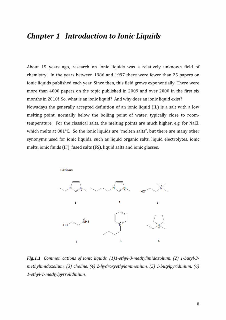
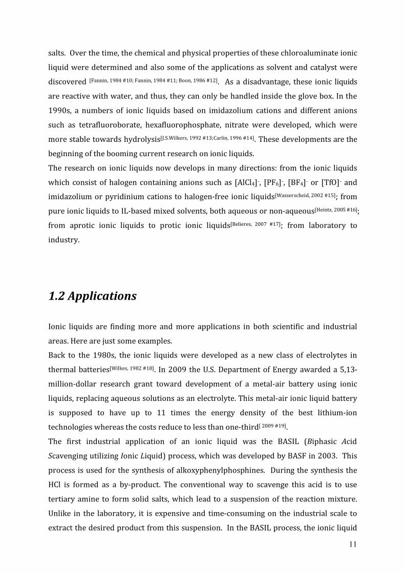
Fig.1.1 Common cations of ionic liquids. (1)1-ethyl-3-methylimidazolium, (2) 1-butyl-3-
methylimidazolium, (3) choline, (4) 2-hydroxyethylammonium, (5) 1-butylpyridinium, (6)
1-ethyl-1-methylpyrrolidinium.
9
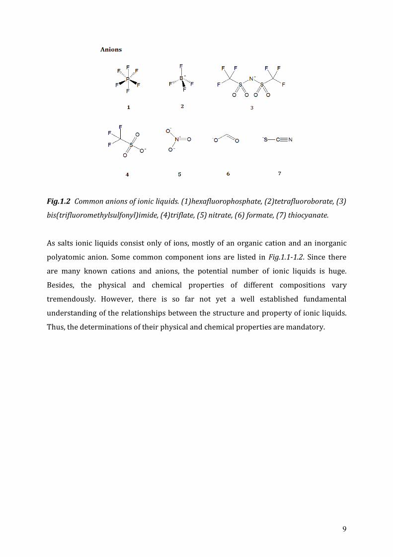
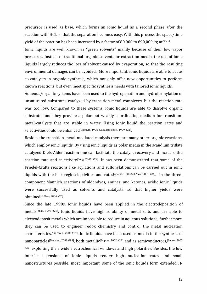
Fig.1.2 Common anions of ionic liquids. (1)hexafluorophosphate, (2)tetrafluoroborate, (3)
bis(trifluoromethylsulfonyl)imide, (4)triflate, (5) nitrate, (6) formate, (7) thiocyanate.
As salts ionic liquids consist only of ions, mostly of an organic cation and an inorganic
polyatomic anion. Some common component ions are listed in Fig.1.1-1.2. Since there
are many known cations and anions, the potential number of ionic liquids is huge.
Besides, the physical and chemical properties of different compositions vary
tremendously. However, there is so far not yet a well established fundamental
understanding of the relationships between the structure and property of ionic liquids.
Thus, the determinations of their physical and chemical properties are mandatory.
10
1.1 History Ionic liquids can be viewed as materials with a long history. The first ionic liquid
reported in the literature was ethanol-ammonium nitrate with a melting point of 52-55
°C, which was synthesized by S. Gabriel and J. Weiner in 1888[Gabriel, 1888 #1]. One of the
earliest truly room temperature ionic liquids was ethyl-ammonium nitrate with the
melting point of 12 °C, synthesized in 1914 by Paul Walden[Walden, 1914 #2]. Another key
step in ionic liquid research was the work of J. Yoke at Oregon State University in 1960s.
He found that solid copper(I) chloride and alkyl ammonium chloride formed a liquid at
room temperature when they were mixed together[Yoke, 1963 #3]. In the 1970s Jerry
Atwood and his group at the University of Alabama discovered and characterized a
series of unusual compounds, which were denoted as liquid clathrates. These
compounds are composed of a salt with an aluminium alkyl compound and one or more
aromatic molecules. They are now recognized as ionic liquids, but not strictly because of
the aromatic molecules[J.D.Atwood, 1976 #4;J.L.Atwood, 4 496 744`,1981 #5]. All these works form the
very first story of ionic liquids, but none of these materials was direct related to the
presently used generation of ionic liquids.
The impetus of the present developments was the problem of using high temperature
molten salts in the thermal batteries. Some 40 years ago, these traditional
chloroaluminate molten salts, such as LiCl or KCl mixed with AlCl3, were called ‘low
temperature molten salts’. They were used as electrolytes and were heated by
pyrotechnic procedures, when the batteries were activated. With a temperature of 375-
550°C, these batteries were just too hot to handle. To develop a molten salt electrolyte
operated at a much lower temperature was the goal of an Air Force Academy group in
the 1960s and 1970s. Lowell A. King chose the little-known alkali chloride-aluminium
chloride system [John, 2002 #6].
In 1978, the chemical and physical properties of a 1-butylpyridinium chloride-
aluminium chloride mixture (BPC-AlCl3) were measured and published[R.J.Gale, 1978
#7;J.C.Nardi, 4 122 245`, 1978 #8], which is marked as a start of the modern era of ionic liquids,
because for the first time a wider audience of chemists started to take interest in these
totally ionic, completely nonaqueous new solvents [John, 2002 #6;Peter, 2008 #9]. However, BPC-
AlCl3 is not a room-temperature liquid (Mp. 40°C) and the alkylpyridinium cation is
relatively easy to reduce[John, 2002 #6]. More attractive candidates are dialkylimidazolium
11
salts. Over the time, the chemical and physical properties of these chloroaluminate ionic
liquid were determined and also some of the applications as solvent and catalyst were
discovered [Fannin, 1984 #10; Fannin, 1984 #11; Boon, 1986 #12]. As a disadvantage, these ionic liquids
are reactive with water, and thus, they can only be handled inside the glove box. In the
1990s, a numbers of ionic liquids based on imidazolium cations and different anions
such as tetrafluoroborate, hexafluorophosphate, nitrate were developed, which were
more stable towards hydrolysis[J.S.Wilkers, 1992 #13;Carlin, 1996 #14]. These developments are the
beginning of the booming current research on ionic liquids.
The research on ionic liquids now develops in many directions: from the ionic liquids
which consist of halogen containing anions such as [AlCl4]-, [PF6]-, [BF4]- or [TfO]- and
imidazolium or pyridinium cations to halogen-free ionic liquids[Wasserscheid, 2002 #15]; from
pure ionic liquids to IL-based mixed solvents, both aqueous or non-aqueous[Heintz, 2005 #16];
from aprotic ionic liquids to protic ionic liquids[Belieres, 2007 #17]; from laboratory to
industry.
1.2 Applications Ionic liquids are finding more and more applications in both scientific and industrial
areas. Here are just some examples.
Back to the 1980s, the ionic liquids were developed as a new class of electrolytes in
thermal batteries[Wilkes, 1982 #18]. In 2009 the U.S. Department of Energy awarded a 5,13-
million-dollar research grant toward development of a metal-air battery using ionic
liquids, replacing aqueous solutions as an electrolyte. This metal-air ionic liquid battery
is supposed to have up to 11 times the energy density of the best lithium-ion
technologies whereas the costs reduce to less than one-third[ 2009 #19].
The first industrial application of an ionic liquid was the BASIL (Biphasic Acid
Scavenging utilizing Ionic Liquid) process, which was developed by BASF in 2003. This
process is used for the synthesis of alkoxyphenylphosphines. During the synthesis the
HCl is formed as a by-product. The conventional way to scavenge this acid is to use
tertiary amine to form solid salts, which lead to a suspension of the reaction mixture.
Unlike in the laboratory, it is expensive and time-consuming on the industrial scale to
extract the desired product from this suspension. In the BASIL process, the ionic liquid
12
precursor is used as base, which forms an ionic liquid as a second phase after the
reaction with HCl, so that the separation becomes easy. With this process the space/time
yield of the reaction has been increased by a factor of 80,000 to 690,000 kg m-3 h-1.
Ionic liquids are well known as “green solvents” mainly because of their low vapor
pressures. Instead of traditional organic solvents or extraction media, the use of ionic
liquids largely reduces the loss of solvent caused by evaporation, so that the resulting
environmental damages can be avoided. More important, ionic liquids are able to act as
co-catalysts in organic synthesis, which not only offer new opportunities to perform
known reactions, but even meet specific synthesis needs with tailored ionic liquids.
Aqueous/organic systems have been used to the hydrogenation and hydroformylation of
unsaturated substrates catalyzed by transition-metal complexes, but the reaction rate
was too low. Compared to these systems, ionic liquids are able to dissolve organic
substrates and they provide a polar but weakly coordinating medium for transition-
metal-catalysts that are stable in water. Using ionic liquid the reaction rates and
selectivities could be enhanced[Chauvin, 1996 #20;Carmichael, 1999 #21].
Besides the transition-metal-mediated catalysis there are many other organic reactions,
which employ ionic liquids. By using ionic liquids as polar media in the scandium triflate
catalyzed Diels-Alder reaction one can facilitate the catalyst recovery and increase the
reaction rate and selectivity[Song, 2001 #22]. It has been demonstrated that some of the
Friedel-Crafts reactions like acylations and sulfonylations can be carried out in ionic
liquids with the best regioselectivities and rates[Adams, 1998 #23;Nara, 2001 #24]. In the three-
component Mannich reactions of aldehdyes, amines, and ketones, acidic ionic liquids
were successfully used as solvents and catalysts, so that higher yields were
obtained[G.Zhao, 2004 #25] .
Since the late 1990s, ionic liquids have been applied in the electrodeposition of
metals[Zhao, 1997 #26]. Ionic liquids have high solubility of metal salts and are able to
electrodeposit metals which are impossible to reduce in aqueous solutions; furthermore,
they can be used to engineer redox chemistry and control the metal nucleation
characteristics[Andrew P., 2006 #27]. Ionic liquids have been used as media in the synthesis of
nanoparticles[Mudring, 2009 #28], both metallic[Dupont, 2002 #29] and as semiconductors,[Endres, 2002
#30] exploiting their wide electrochemical windows and high polarities. Besides, the low
interfacial tensions of ionic liquids render high nucleation rates and small
nanostructures possible; most important, some of the ionic liquids form extended H-
13
bonded systems, and these highly structured liquids have a strong effect on the
morphology of the nanoscale structures.
Currently, ionic liquids are widely applied in most sub-disciplines of analytical
chemistry, including extraction[Liu, 2009 #31], gas chromatography[Yao, 2009 #32], liquid
chromatography and capillary electrophoresis[Berthod, 2008 #33], sensors[A.Kamio, 2008 #34], and
as matrixes in MALDI mass spectrometry[J.A.Crank;D.W.Armstrong, 2009 #35] or as pairing reagents
in ESI-MS[R.J.Soukup-Hein, 2007 #36].
In polymer science, ionic liquids are used as plasticizers and solvents for polymerization
processes and as key components in new classes of polymer gels[Jianmei Lu, 2009 #37].
Supercapacitors are energy storage and conversion systems of high power for many
applications. Equipped with ionic liquids as solvent-free electrolytes, safe high-energy
supercapacitors can prevent from sacrificing power capability and cycling
stability[Mastragostino, 2009 #38].
Because of their unusual solvation characteristics, ionic liquids are proposed to be
unique solvents for biomolecules such as proteins. They are used as media for
biocatalytic reactions[Peter, 2008 #9], biosensors[H.Ohno, 2003 #39], protein stabilizations[S.N.Baker,
2004 #40;Constantinescu, 2009#41] and biopreservation[P.Majewski, 2003 #42]. In biomedicine, ionic
liquids are considered to have potential to advance formulation science for protein-
based pharmaceutical preparations and cellular therapies[Elliott Gloria, 2009 #43].
Other applications of ionic liquids include robust electrolytes for photoelectrochemical
cells, such as dye-sensitized solar cell[Grätzel, 2009 #44]. In another interesting application
the ionic liquid is coated with colloidal silver particles to become a highly reflective
material that could be used as a liquid mirror of a space telescope[Borra, 2007 #45].
More applications and recent research on the development of ionic liquids can be found
in the book of “Ionic Liquids in Synthesis”, “Ionic Liquids: From Knowledge to
Application” and “An Introduction to Ionic Liquids”. [Peter, 2008 #9][Natalia V. Plechkova, 2009
#168][Freemantle, 2010 #169]
1.3 Synthesis The preparation of ILs presents no significant difficulties, even in large quantities. For
non-protic ILs, the synthesis requires generally two steps: the alkylation of a tertiary
amine by alkyl halide, followed by the exchange of the halide anion with the
14
corresponding anion to get the desired product[Mickiko Hirao, 2000 #46]. Protic ionic liquids are
formed by proton transfer between a Brönsted acid and a Brönsted base through the
acid-base neutralization reaction[Angell, 2007 #47].
Since the presence of certain impurities can lead to a radical change of the
chemophysical properties, the purification of ionic liquids is always an important part of
the synthesis. The impurities can be the compounds originating from starting materials
through oxidation or thermal degradation, the unreacted starting materials, halide
impurities, acidic impurities, and water, which is the most common impurity in ILs, even
in hydrophobic ones. [Peter, 2008 #9]
To minimize the impurities, there are some options. First, the use of clean materials,
which means all the starting materials should be purified before synthesis; second, the
reaction should be carried out under inert gas such as nitrogen; third, the reaction
temperature should be kept as low as possible, especially for the acid-base
neutralization; finally, one has to dry the ILs after the synthesis, e.g. over a week in cold
trap with vacuum pump, and before the direct use, normally at 70°C in vacuum for 48
hours.
1.4 Chemical and physical properties Ionic liquids are receiving more and more interest because of their unique properties.
Based on these properties, a multitude of applications is being developed. Although
ionic liquids are applied in many fields and considered to be very potential to meet the
special needs for different projects, the lack of systematic and mechanistic
understanding of the properties is a bottleneck for progress. However, the research on
ionic liquids is still in the early stage, and for the most common used ionic liquids, some
properties are now widely examined.
15
1.4.1 Thermal properties
1.4.1.1 Measurement technique
The most common techniques which are used to measure the thermal properties of a
material are differential scanning calorimetry (DSC) and thermogravimetric analysis
(TGA).
DSC measures the difference of heat, which is required to increase the temperature of a
sample and a reference as a function of temperature. Using this technique, phase
transitions such as fusion, crystallization and the glass transition can be observed. The
principle of this technique is that, for phase transitions, the sample and different
amounts of heat will be needed to establish the same temperature, more by exothermic
process such as fusion, less by endothermic process such as crystallization. An
alternative to DSC is differential thermal analysis (DTA), in which same heat flow is
enforced instead the same end temperature. Similar information is provided by both
DSC and DTA.
TGA measures the changes in weight of sample in relation to temperature. It is widely
used to determine the degradation, absorbed moisture content, and the decomposition
points.
It is always benefitial to combine both techniques, DSC and TGA, to get the thermal
information about materials, and interpretation of the results is easier.
1.4.1.2 Melting, Crystallization and glass-transition temperatures
The thermal behaviors of ILs are complex and can be largely different. ILs have by
definition a melting point below 100°C; actually they cover a broad range of melting
temperature, from below room temperature to above 100°C. The combination of Volume
Based Thermodynamics (VBT) and quantum chemical calculations can be used for
understanding of the low melting points of ILs compared to classical salts[Ingo Krossing, 2007
#48;Weingärtner, 2008 #49]. At the melting temperature, the Gibbs free energy of fusion ΔfusGm is
zero; for a given temperature, the sign of ΔfusGm indicates the favored state: positive for
solid and negative for liquid. The Born-Fajans-Haber cycle provides basic insights into
the processes that control the phase transition. ΔfusGm equals the sum of the Gibbs
16
energy of lattice ΔlattGm and the Gibbs energies of solvation of cation and anion,
ΔsolvGm(A+) and ΔsolvGm(X-) in the IL. At room temperature negative ΔfusGm result from
small lattice enthalpies and large entropy changes, indicate that the favored liquid state
comes from large size and conformational flexibility of the ions.
Many factors have been discussed that influence the melting points [H.Ohno, 2002 #50;Urszula
Domanska, 2005 #51;H.Ohne, 2004 #52;Dzyuba, 2002 #53] of ILs. The dominant force in ILs is the
Columbic attraction between ions. The lattice energy of ionic solids depends on the
product of net ion charges, the ion-ion separation and the packing efficiency of the ions.
Change in size, shape and character of the component ions influences the melting
temperature. Generally, large ions tend to lower the melting points, e.g. for [EtMeIm]X-
Tm decreases in the series [Cl]->[NO3]->[BF4]->[Tf2N]-[H.Ohno, 2006#54] and for
tetraalkylammonioum bromide salts, Tm decreases with increasing cation size[Peter, 2008 #9].
Also the shape of the ions is important: increasing the symmetry of the ions or changing
from planar ions to spherical ions increases Tm by enabling more efficient ion-ion
packing in the crystal cell, which, for example, renders Tm of imidazolium salts lower
than of tetraalkylammonioum salts. For the imidazolium ionic liquids with alkyl chains
[CnMeIm]+, Tm decreases with increasing chain length for 4<n<12; for n>12, Tm starts to
increase with increasing chain length and the phase diagrams become complicated.
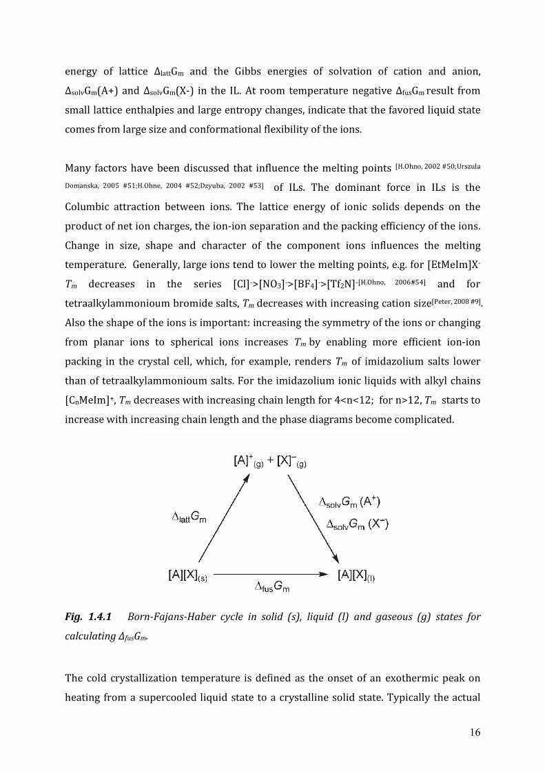
Fig. 1.4.1 Born-Fajans-Haber cycle in solid (s), liquid (l) and gaseous (g) states for
calculating ΔfusGm.
The cold crystallization temperature is defined as the onset of an exothermic peak on
heating from a supercooled liquid state to a crystalline solid state. Typically the actual
17
crystallization temperatures of ILs are 30-60K lower than equilibrium melting points,
which indicates a slow crystallization rate and a fairly stable supercooled state[H.Tokuda,
2004 #55;H.Jin, 2008 #56]. For the ILs with low melting points, the crystallization is not very
favoured because of the low lattice energy mentioned above. Instead cooling ILs from
the liquid state to a low temperature causes glass formation, which preferably happens
by rapid cooling. The glass transition is indicative of the cohesive energy within the IL,
which is decreased by repulsive Pauli forces and increased by the attractive Coulomb
and van der Waals interactions[Xu, 2003 #57]. Through the modification of the cation and
anion component can usually influence the glass temperature like melting point. For
most of the ILs, the glass temperatures are very low, varies from -20 to -120°C.
Concern about the phase transition, three types of the behavior could be summarized.
First kind of ILs have distinct freezing point on cooling and melting point on heating;
crystallize with no glass formation, e.g. [BuMeIm][TfO]. The second kind of ILs has no
true phase transitions. On cooling there only forms an amorphous glass, upon heating
the liquid is recovered, and there is no well-defined melting point or freezing point, e.g.
in [BuMeIm][Br]. The third group of ILs form glasses by supercooling and crystallize by
heating, followed by a melting transition, e.g. [BuMeIm][PF6]. [C.P.Fredlake, 2004 #58]
1.4.1.3 Decomposition Temperature
To determine the thermal stabilities of ILs thermogravimetric analysis (TGA) can be
used. Very little weight loss before decomposition confirms the negligible vapour
pressures of ILs, which facilitates their handling as solvents and forms one of the basic
requirements for the “green” nature. Traditional molten salts form tight ion pairs in the
vapour phase; in contrast, the ion pair formation in the ILs is energetically restricted
because of the reduced Columbic interactions, which leads to low vapour pressures of
ILs. Therefore the decomposition temperatures of ILs are usually related to the upper
limit of their liquid range.
A lot of decomposition temperatures Td of ILs were determined[M.kosmulski, 2003 #59;H.L.Ngo,
2000 #60;C.Drummond, 2008 #61], usually up to 500°C. Table 1.4.1 lists decomposition
temperatures of some ILs. In fact, thermal decomposition is strongly dependent on the
structure of ILs and varies with different cation-anion combination. Generally it can be
concluded:
18
i) Compared to ammonium cations the imidazolium cations tend to be thermally more
stable, e.g. Td of [BuMeIm][BF4] is 403°C, whereas Td of [BuMeNH2][BF4] is 350°C and Td
of [tert-BuNH3][BF4] is 243°C;
ii) The thermal stability of the imidazolium salts increases with increasing linear alkyl
substitution;
iii) Variation of the anion types follow the relative stabilities: [PF6]- > [Tf2N]- > [BF4]->
[Br]-> [Cl]-, e.g. Td of [EtMeIm][Br] is 311°C and Td of [EtMeIm][Cl] is 281°C;
iv) Protic ILs have generally lower Td than non-protic ILs because of the shifts in the
proton transfer equilibrium between the salt form and acid/base pairs, e.g.
[BuMeIm][Tf2N] with 423°C and [BuNH3][Tf2N] with 352°C. Td of tributylammonium
nitrate is even as low as 120°C .
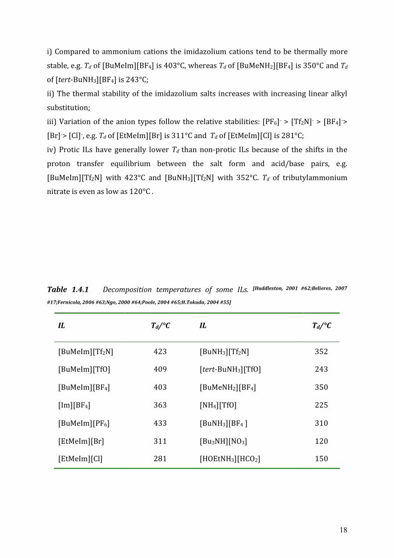
Table 1.4.1 Decomposition temperatures of some ILs. [Huddleston, 2001 #62;Belieres, 2007
#17;Fernicola, 2006 #63;Ngo, 2000 #64;Poole, 2004 #65;H.Tokuda, 2004 #55]
IL Td/°C IL Td/°C
[BuMeIm][Tf2N] 423 [BuNH3][Tf2N] 352
[BuMeIm][TfO] 409 [tert-BuNH3][TfO] 243
[BuMeIm][BF4] 403 [BuMeNH2][BF4] 350
[Im][BF4] 363 [NH4][TfO] 225
[BuMeIm][PF6] 433 [BuNH3][BF4 ] 310
[EtMeIm][Br] 311 [Bu3NH][NO3] 120
[EtMeIm][Cl] 281 [HOEtNH3][HCO2] 150
19
1.4.2 Viscosity and self-diffusion coefficient
Fluids resist the relative motion of immersed objects as well as to the motion of layers
with differing velocities within them. Viscosity is the internal property of a fluid that
describes resistance to flow. There are two quantities that are called viscosity: the
dynamic viscosity (η) is expressed in SI units of Pascal times second (Pa·s) or in the older
cgs system in poise (P) (1P = 0.1Pa·s), By contrast the kinematic viscosity (υ) is
expressed in the SI systems in terms of m2/s or in the cgs systems in terms of Stokes (St)
(1 St = 10−4 m2·s−1). The relationship between dynamic viscosity (η) and kinematic
viscosity (υ) and density (ρ) is as follows:
(1.4.1)
Formally, the viscosity is the ratio of the shearing stress, which is the pressure exerted
on the surface of a fluid in the lateral or horizontal direction, to the velocity gradient in a
fluid. For straight, parallel and uniform flow, the shear stress between layers is
proportional to the velocity gradient in the vertical direction to the layers; the constant
of proportionality is the fluid viscosity. The fluids with this kind of behaviour are called
Newtonian fluid (named after Isaac Newton). By contrast, non-Newtonian fluids have a
more complicated relationship between shear stress and velocity gradient than simple
linearity. Many fluids are Newtonian type, such as water, hydrocarbons and oils; fluids
like polymer solutions, blood, and ketchup are non-Newtonian. The popular ILs are
recognized as Newtonian fluids, and there are no data so far for non-Newtonian ILs.
1.4.2.1 Measurement methods
There are three major measurement methods to determine the viscosity of ILs based on
falling balls, capillary flow and rotational techniques. The construction of a falling ball
viscometer can be easily described as a vertical glass tube and a ball with known size
and density. In the measurement the ILs to be examined are filled into the glass tube and
stay stationary in the tube; the ball is dropped carefully through the IL. With a correct
selection, the ball reaches its terminal velocity, which can be measured by the time it
20
takes to pass two marks on the tube. Using Stroke’s Law the dynamic viscosity of IL can
be calculated:
2
92 gRs
(1.4.2)
ρs is the density of the ball, ρ is the density of the IL, g is the gravity constant, R is the
radius of the ball, υ is the terminal velocity of the ball. Commonly, the falling ball
viscometer is calibrated with a standard fluid which has a similar viscosity to the IL of
interest to get an instrument constant k; the kinematic viscosity of IL is then given by:
sk (1.4.3)
θ is the falling time between two marks on the glass tube. Generally the falling ball
viscometer is used for the ILs in the viscosity range of 10-3 to 107 P.[2000 #66]
The glass capillary viscometer is also known as U-tube viscometer or Ostwald
viscometer. It consists of a glass U-tube with a capillary section between two bulbs, one
is higher on one arm, and the other one is lower down one another arm. In the
measurement the fluid is drawn into the upper bulb using a vacuum, then allowed to
flow down through the capillary into the lower bulb. The time required for the test
liquid to flow through the capillary between two marked points is measured. The
kinematic viscosity can be calculated using:[2000 #66]
tLV
Dzzg
0
421
128 (1.4.4)
where (z1-z2) is the change of the height, D is the capillary inner diameter, L is the length
of the capillary, and V0 is the volume between the fiducial marks. With known density of
the fluid the dynamic viscosity can also be calculated. This kind of viscometer is used for
the ILs with the viscosity range of 4∙10-3 to 1.6∙102 St or 6∙10-3 to 2.4∙102 P.
The last widely used viscometer is the rotational viscometer. The idea of this kind of
viscometer is that the torque required to turn an object in a fluid is a function of the
viscosity of that fluid. Two main elements of rotational viscometer are a rotating
element and a fixed element, which could be concentric cylinders, cone and plate and
parallel disks. By measurement the test fluid is placed in the space between the two
21
elements and the torque transferred is measured, and then the viscosity of the fluid can
be calculated. Take the concentric cylinder as an example:
2
22
2
41
T
LR e
(1.4.5)
where β is the ratio of the cylinder radii, R2 is the radius of the outer cylinder, Le is the
effective length of the cylinder, T is the torque, and ω2 is the rotational speed of the outer
cylinder.
1.4.2.2 Viscosity of ionic liquids
Viscosity is a key transport property of ionic liquids, which has a great influence on the
rate of mass transport. High viscosities form barriers for many of their applications and
slow down the rate of the chemical reactions, which are diffusion controlled. As a group,
ILs tend to have higher viscosities than conventional molecular solvents, and the value
of the viscosity varies tremendously with chemical structure, composition, temperature
and the presence of solutes of impurities. At room temperature, the viscosities of ILs
range from low to 5 cP to more than 1000 cP. Some viscosities are listed in the table
1.4.2.
Table 1.4.2 Viscosities of some ILs compared with water and organic solvents at room-
temperature. [1992-1993 #67; Seddon Kenneth, 2002 #68]
IL η / cP Liquid η / cP
[EtMeIm][BF4] 67 water 0.894
[EtMeIm][PF6] 371 ethanol 1.074
[HeMeIm][NO3] 804 castor oil 985
[HeMeIm][Cl] 18000 glycerol 1490
22
As mentioned above, there are many factors that influence the viscosities of ILs. First of
all is the temperature. The viscosity of a liquid decreases as the temperature increases.
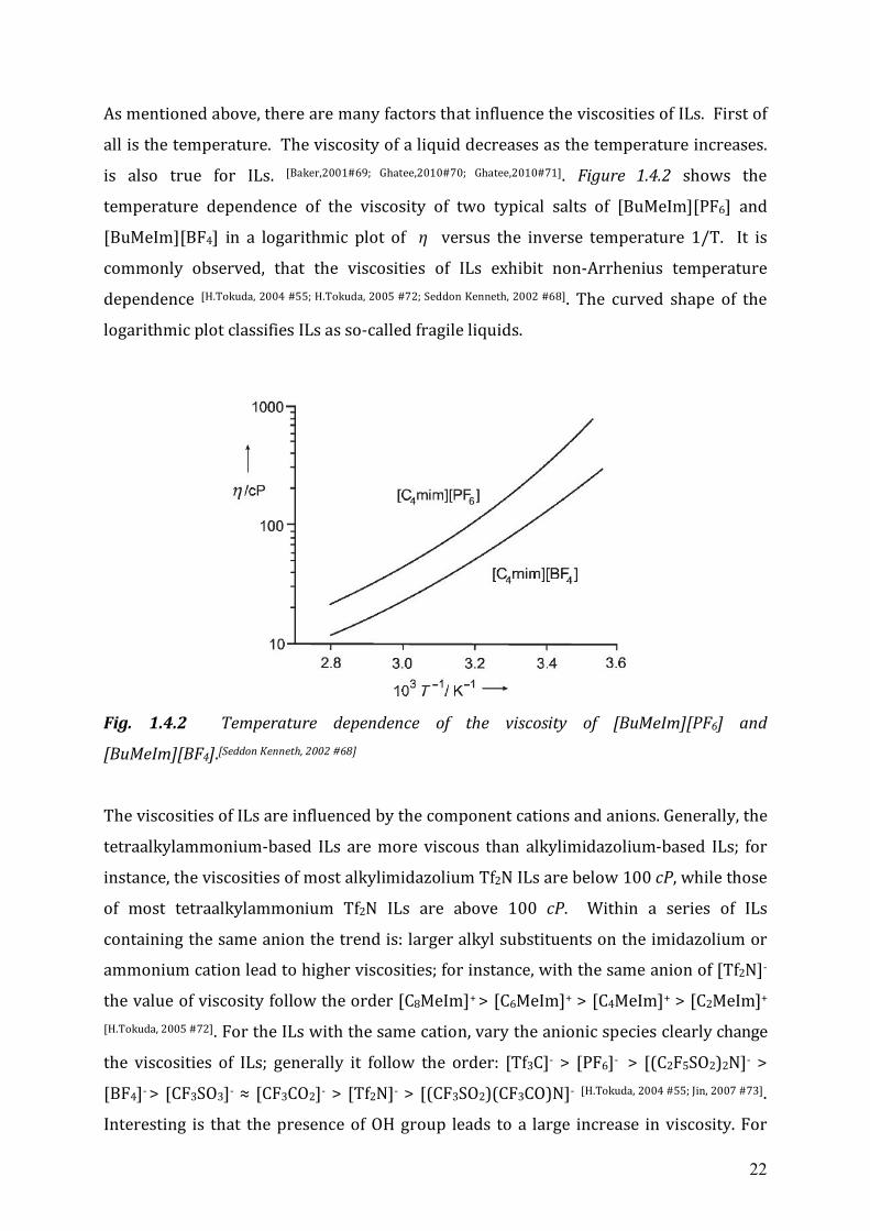
is also true for ILs. [Baker,2001#69; Ghatee,2010#70; Ghatee,2010#71]. Figure 1.4.2 shows the
temperature dependence of the viscosity of two typical salts of [BuMeIm][PF6] and
[BuMeIm][BF4] in a logarithmic plot of η versus the inverse temperature 1/T. It is
commonly observed, that the viscosities of ILs exhibit non-Arrhenius temperature
dependence [H.Tokuda, 2004 #55; H.Tokuda, 2005 #72; Seddon Kenneth, 2002 #68]. The curved shape of the
logarithmic plot classifies ILs as so-called fragile liquids.
Fig. 1.4.2 Temperature dependence of the viscosity of [BuMeIm][PF6] and
[BuMeIm][BF4].[Seddon Kenneth, 2002 #68]
The viscosities of ILs are influenced by the component cations and anions. Generally, the
tetraalkylammonium-based ILs are more viscous than alkylimidazolium-based ILs; for
instance, the viscosities of most alkylimidazolium Tf2N ILs are below 100 cP, while those
of most tetraalkylammonium Tf2N ILs are above 100 cP. Within a series of ILs
containing the same anion the trend is: larger alkyl substituents on the imidazolium or
ammonium cation lead to higher viscosities; for instance, with the same anion of [Tf2N]-
the value of viscosity follow the order [C8MeIm]+ > [C6MeIm]+ > [C4MeIm]+ > [C2MeIm]+
[H.Tokuda, 2005 #72]. For the ILs with the same cation, vary the anionic species clearly change
the viscosities of ILs; generally it follow the order: [Tf3C]- > [PF6]- > [(C2F5SO2)2N]- >
[BF4]- > [CF3SO3]- ≈ [CF3CO2]- > [Tf2N]- > [(CF3SO2)(CF3CO)N]- [H.Tokuda, 2004 #55; Jin, 2007 #73].
Interesting is that the presence of OH group leads to a large increase in viscosity. For
23
example, at 25°C the viscosity of [BuMeIm][Tf2N] is 49 cP and the viscosity of
[HOEtMeIm][Tf2N] is almost doubled to 91 cP; with two OH groups the effect is much
more dramatic: compare the N-propyl-N-methylpyrrolidinium Tf2N with 54 cP and N-
1,2-propanediol-N-methyl-pyrrolidinium Tf2N with 1500 cP. [Jin, 2007 #73]
1.4.2.3 Self diffusion coefficient
According to IUPAC definition, self-diffusion coefficient is the diffusion coefficient Di* of
species i when the chemical potential gradient equals zero. It is linked to the diffusion
coefficient Di by the equation:
i
iii a
cDDlnln*
(1.4.6)
where ai is the activity of the species i in the solution and ci is the concentration of i.
For ILs, the pulsed gradient spin echo PGSE-NMR is a common method used to
determine the self-diffusion coefficient, which allows evaluation of the diffusivity of ions
without the use of additional probe molecules.
For the diffusion of a sphere of radius r in a hydrodynamic continuum of viscosity η, the
diffusion–viscosity relationship is often described by the Stokes–Einstein (SE) equation:
r
TkD B
(1.4.7)
The coupling factor ξ accounts for the different hydrodynamic boundary conditions at
the interface between the diffusing sphere and the viscous medium.
In low-viscosity ILs at 25°C, the self-diffusion coefficients of the cations and anions are of
the order of 10-11 m2 s-1. Those of simple molecular liquids are of the order of 10-9 -10-10
m2 s-1[H.Tokuda, 2005 #72; H.Tokuda, 2004 #55]. The self-diffusion coefficients are also temperature
dependent; the values decrease with the increasing temperature. With the same anion,
e.g. [Tf2N]-, the sum of the cationic and anionic diffusion coefficients for the imidazolium-
based ILs follows the order: [C2MeIm]+ > [C1MeIm]+ > [C4MeIm]+ > [C6MeIm]+ >
24
[C8MeIm]+ ; with the same cation, e.g. [BuMeIm]+, the sum follows the order:
[(CF3SO2)2N]- > [CF3CO2]- > [CF3SO3]- > [BF4]- > [PF6]- .
1.4.3 Polarity
In the chemical reactions, solvent effects are widely discussed and have powerful
influence on the rate, equilibria and outcome of the reactions. Thus the choice of the
right solvent for the reaction is a key topic. One of the most important properties, which
classify the solvents, is the polarity. As a “designer solvent”, the polarity of an IL also
helps to predict the solubility, miscibility and distribution equilibria. However, the
solvent polarity describes the global solvation capability, which results from complex
molecular interactions. There are many experimental methods to characterize the
solvation polarity, each scale highlights different facet of these interactions. Some
methods are listed as followed and more discussions about these methods are followed
in the next two chapters.
- Dielectric spectroscopy
- Absorption spectra
- Fluorescence spectra
- Electron spin resonance spectroscopy
- Chromatography
- Solvent effects upon chemical reactions
The most common scale used to describe the polarity is the static dielectric constant (εs).
Because the direct measurement of εs requires a non-conducting medium, which for ILs
is not available, conventional methods are not suitable for the measuring of εs of ILs.
However, through the measuring of frequency dependent dielectric permittivity and
extrapolation to zero frequency the dielectric constants of electrolyte solutions can be
determined. As discussed earlier, most ILs are fluids of relatively low viscosity. Then, the
frequency-dependent behaviour falls into microwave range, from about 100MHz to
25
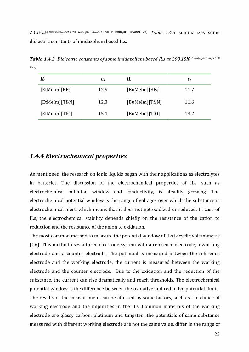
20GHz.[S.Schrodle,2006#74; C.Daguenet,2006#75; H.Weingärtner,2001#76] Table 1.4.3 summarizes some
dielectric constants of imidazolium based ILs.
Table 1.4.3 Dielectric constants of some imidazolium-based ILs at 298.15K[H.Weingärtner, 2009
#77]
IL εs IL εs
[EtMeIm][BF4] 12.9 [BuMeIm][BF4] 11.7
[EtMeIm][Tf2N] 12.3 [BuMeIm][Tf2N] 11.6
[EtMeIm][TfO] 15.1 [BuMeIm][TfO] 13.2
1.4.4 Electrochemical properties
As mentioned, the research on ionic liquids began with their applications as electrolytes
in batteries. The discussion of the electrochemical properties of ILs, such as
electrochemical potential window and conductivity, is steadily growing. The
electrochemical potential window is the range of voltages over which the substance is
electrochemical inert, which means that it does not get oxidized or reduced. In case of
ILs, the electrochemical stability depends chiefly on the resistance of the cation to
reduction and the resistance of the anion to oxidation.
The most common method to measure the potential window of ILs is cyclic voltammetry
(CV). This method uses a three-electrode system with a reference electrode, a working
electrode and a counter electrode. The potential is measured between the reference
electrode and the working electrode; the current is measured between the working
electrode and the counter electrode. Due to the oxidation and the reduction of the
substance, the current can rise dramatically and reach thresholds. The electrochemical
potential window is the difference between the oxidative and reductive potential limits.
The results of the measurement can be affected by some factors, such as the choice of
working electrode and the impurities in the ILs. Common materials of the working
electrode are glassy carbon, platinum and tungsten; the potentials of same substance
measured with different working electrode are not the same value, differ in the range of
26
±0.2 V. The impurities in ILs can have a pronounced impact on the electrochemical
window. For example, the potential of vacuum dried [BuMeIm][Tf2N] is 4.3 V, whereas
without drying is 2.9 V; the dried [BuMeIm][BF4] is 5.1 V, without drying is 4.0 V[O’Mahony,
2008 #78].
With the variation of the component cations and anions, the electrochemical windows of
ILs change to a certain extent, from about 2 V to over 6 V. Comparison of ILs with
similar anions, the electrochemical stability of cations follows the order: pyridinium <
imidazolium < sulfonium < pyrrolidinium < ammonium [S.Yeon, 2005 #79; T.Sato, 2004 #80; Z.Zhou,
2005 #81]. Because of the uncertainties by the measurements, the effect of the changing
alkyl substituents on the electrochemical window of cations is difficult to determine;
however, for the imidazolium-based ILs, when the 2-position of the imidazolium ring is
capped by an alkyl group, the stability of the cation increases clearly. It is proposed that
the limiting reaction of the imidazolium cations is the reduction of ring protons to
molecular hydrogen[G.Gray, 1996 #82], and the 2-position is the most acidic hydrogen; the
substitution of the alkyl group at that position actually improve the reductive stability of
the imidazolium cation. The anion stability towards oxidation follows the order: halides
(Cl-,F-,Br-) < fluorinated ions ([PF6]-) < triflate/triflyl ions ([CF3SO2]-, [(CF3SO2)2N]-,
[(C2F5SO2)2N]-, [(CF3SO2)3C]-) ≈ fluoroborates ([BF4]-) [S.Yeon, 2005 #79; T.Sato, 2004 #80; Z.Zhou, 2005
#81].
The ionic conductivities of ILs play an important role in their electrochemical
applications. The most common determine technique for the ILs is the impedance
bridge, which uses a two-electrode cell to carry out the measurements. The conductivity
of an electrolyte shows the available charge carriers and their mobility. Although ILs are
composed entirely of ions, their conductivities are not that high as expected. Possible
explanations could be the ion pairing, ion aggregation and reduced ion mobility due to
the large ion size. Generally the conductivities of ILs at room temperature fall into the
range of ~20 mS cm-1; exceptions are ILs with the [(HF)2.3F]- anion, which have the
conductivities at room temperature higher than 100 mS cm-1. Unlike other properties,
the conductivities of ILs are not clearly correlated to the type and size of the ions. Large
size of cation leads to lower conductivity probably due to the reduced mobility; in case
of anion, there is no clear relationship between the size and conductivity.
27
The electrical conductivity is strongly dependent on temperature, so is that of ILs, too.
With increasing temperature, the conductivities of ILs rise and often exhibit classical
Arrhenius behaviour above room temperature. The degree of change in conductivity
with temperature varies depending on the ionic liquids.
Through Walden’s rule, the conductivity and viscosity are often combined:
constant (1.4.8)
where Λ is the molar conductivity given by:
Mk (1.4.9)
where k is the absolute conductivity, M is the molecular weight and the ρ is the density.
Ideally, the Walden Product (Λη) remains constant for a given ionic liquid, regardless of
temperature. With increasing size of cation, the Walden product decreases; the size of
anion shows no clear correlation to the Walden product. Plotting the molar conductivity
(Λ) instead the absolute conductivity can normalize the effects of molar concentration
and density on the conductivity, and give a better indication of the number of mobile
charge carriers in an ionic liquid. [Peter, 2008 #9]
28
Chapter 2 Polarity Measurement Techniques for Ionic Liquids
It is well known to every chemist that the rates and equilibria of chemical reactions are
solvent-dependent. The selection of an appropriate solvent for a reaction is part of the
chemist’s workmanship. Early in the 1860s, the influence of solvents on the rates of
chemical reactions was discovered by Berthelot and Péan de Saint-Gilles[Berthelot, 1862 #83]
and followed by the work done by Menshutkin in 1890s[Menshutkin, 1890 #84]. The influence
of solvents on the position of chemical equilibrium was noted with the discovery of keto-
enol tautomerism in 1,3-dicarbonyl compounds, which was independently done by
Claisen[Claisen,1896#85], Knorr[Knorr.L.,1896#86] and Wislicenus[Wislicenus,1896#87]. With the
development of modern detection techniques, the solvent effects were characterized for
more and more chemical reactions.
The understanding of these effects relies on the concept of solvent polarity. All these
effects result basically from the different solvation, which depends on the intermolecular
forces between solute and surrounding solvent molecules. The intermolecular forces can
be divided into non-specific forces, such as electrostatic forces arising from the Coulomb
forces between charged ions and dipolar molecules and polarization forces arising from
dipole moments induced in molecules by the nearby ions or dipolar molecules; and
specific forces, such as hydrogen-bonding between hydrogen-bond donor and hydrogen-
bond acceptor, and electron-pair donor/electron-pair acceptor forces.[C. Reichardt, 1994 #88]
Therefore, it is difficult to define the term of solvent polarity. A commonly accepted
definition is the overall solvation capability of solvents, which in turn depends on the
action of all possible intermolecular interactions between solute ions or molecules and
solvent molecules. Thus, the solvent polarity actually cannot be described quantitatively
with single solvent parameters. This leads to the development of various empirical
solvent polarity scales based on carefully selected, well-understood and strongly
solvent-dependent model chemical reactions or spectral absorptions.
In case of ILs, many methods have been applied to determine their solvent polarities.
Some of these techniques will be shortly introduced in this chapter, including the basic
principles behind them and part of the results.
29
2.1 Absorption and fluorescence spectroscopy
It has long been known that the absorption or emission spectra of chemical compounds
could be influenced by the surrounding solvents due to the solvent polarity, which lead
to changes in position, intensity and shape of absorption or emission bands; this
phenomenon is called solvatochromism. With increasing solvent polarity negative
solvatochromism leads to hypsochromic (blue) shift of the absorption band and the
positive solvatochromism leads to bathochromic (red) shift. The polarities of the ground
and exited state of a light-absorbing molecule (chromophore) are different; the change
of solvent polarity will change the solvation of the molecules with different electronic
states and thus the energy gap between these electronic states. When the ground-state
molecules are better stabilized with increasing solvent polarity, it leads to negative
solvatochromism; on the contrast, if the exited-state molecules are better stabilized, it
results in positive solvatochromism.
The solvatochromic effects depend on the chemical structure and the physical
properties of the chromophore and the solvent molecules. Generally, dye molecules
with a large change in their permanent dipole moment upon excitation exhibit a strong
solvatochromism and the ability of the solute to donate or to accept hydrogen bonds to
or from surrounding solvent molecules determines the extent and sign of its
solvatochromism.[C.Reichardt, 1994 #88]
The empirical parameters of solvent polarity measured with absorption or emission
spectroscopy are normally determined by means of solvatochromic compounds. The
first solvatochromic dye used for the numbers of polarity determinations was Nile
Red(1)[Carmichael, 2000 #89], and more and more dyes have been applied, such as Reichardt’s
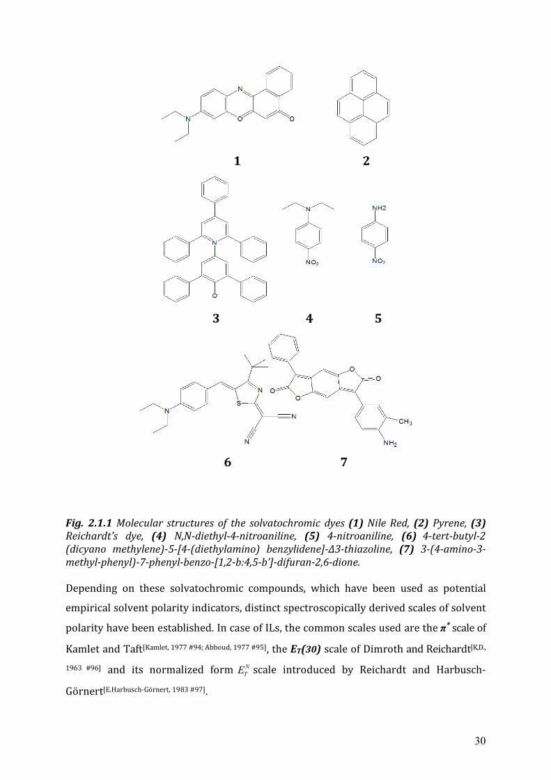
dye(3)[C.Reichardt, 2005 #90;Fletcher, 2001 #91], pyrene(2)[Fletcher, 2001 #91], 4-nitroaniline(5)[L.Crowhurst,
2003 #92], N,N-diethyl-4-nitroaniline(4)[L.Crowhurst, 2003 #92], 3-(4-amino-3-methyl-phenyl)-7-
phenyl-benzo-[1,2-b:4,5-b’]-di furan-2,6-dione(7)[A.Oehlke, 2006 #93], 4-tert-butyl-2-(dicyano
methylene)-5-[4-(diethylamino) benzyl idene]-∆3-thiazoline(6)[A.Oehlke, 2006 #93], which are
shown in Fig.2.1.1.
30
1 2
3 4 5
6 7
Fig. 2.1.1 Molecular structures of the solvatochromic dyes (1) Nile Red, (2) Pyrene, (3) Reichardt’s dye, (4) N,N-diethyl-4-nitroaniline, (5) 4-nitroaniline, (6) 4-tert-butyl-2 (dicyano methylene)-5-[4-(diethylamino) benzylidene]-∆3-thiazoline, (7) 3-(4-amino-3-methyl-phenyl)-7-phenyl-benzo-[1,2-b:4,5-b’]-difuran-2,6-dione. Depending on these solvatochromic compounds, which have been used as potential
empirical solvent polarity indicators, distinct spectroscopically derived scales of solvent
polarity have been established. In case of ILs, the common scales used are the π* scale of
Kamlet and Taft[Kamlet, 1977 #94; Abboud, 1977 #95], the ET(30) scale of Dimroth and Reichardt[K,D.,
1963 #96] and its normalized form NTE scale introduced by Reichardt and Harbusch-
Görnert[E.Harbusch-Görnert, 1983 #97].

31
2.1.1 The π*, α and β scales
Most of the scales are based on data for a single spectral parameter, which are
somewhat inadequate in the correlation analysis of other solvent-dependent processes
because of the complicated solute/solvent interactions. It is known that the empirical
parameters describing solvent polarity can be understood as the result of linear free-
energy relationships[Reichardt, 1979#98]. Kamlet and Taft[Kamlet, 1976#99; Kamlet, 1977#94; Taft, 1976 #100]
established a system, using the solvatochromic comparison of effects on the UV/Vis
spectra of a set of closely related dyes that were selected to test particular solvent
properties. This system includes three parameters, π*, α, and β.
The π* scale is based on solvent-induced shifts of the longest wavelength π → π*
absorption band of nitroaromatic indicators. The electronic transition is connected with
an intramolecular charge transfer from the electron-donor part, such as OMe, NR2, alkyl,
to the electron acceptor part, such as NO2, COC6H5 through the aromatic system.
Therefore, the exited state is more dipolar than the ground state. Seven nitroaromatics
haven been employed in the initial construction of the π* scale and the value was
normalized and averaged to give π*=0.00 for cyclohexane and π*=1.00 for dimethyl
sulfoxide[Kamlet, 1977 #94]. The α- and β - scales are based on the hydrogen-bonding effect.
In case of a solvent as hydrogen-bond acceptor interacting with the dye molecule, such
as 1a in Fig. 2.1.2, an electronic transition from a hydrogen-bonded ground state to an
excited state would lead to a hydrogen-bond strengthening in the electronic excitation
(1b in Fig. 2.1.2), corresponding to a lowering in electronic transition energy, which
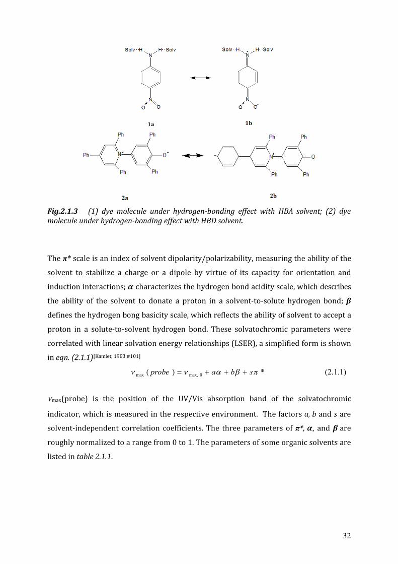
leads to a bathochromic effect.[Kamlet, 1976 #99] In case of a solvent acting as hydrogen-bond
donor to the dye molecule, such as 2a in Fig. 2.1.3, the electronic transition leads to
charge delocalization from the phenoxide oxygen into the pyridinium ring and then to
the attached phenyl groups (2b, Fig.2.1.3). Thus, the hydrogen-bonding to phenoxide
oxygen should stabilize the ground state relative to the excited state, which results in a
hypsochrimic effect.[Taft, 1976 #100]
32
Fig.2.1.3 (1) dye molecule under hydrogen-bonding effect with HBA solvent; (2) dye molecule under hydrogen-bonding effect with HBD solvent.
The π* scale is an index of solvent dipolarity/polarizability, measuring the ability of the
solvent to stabilize a charge or a dipole by virtue of its capacity for orientation and
induction interactions; α characterizes the hydrogen bond acidity scale, which describes
the ability of the solvent to donate a proton in a solvent-to-solute hydrogen bond; β
defines the hydrogen bong basicity scale, which reflects the ability of solvent to accept a
proton in a solute-to-solvent hydrogen bond. These solvatochromic parameters were
correlated with linear solvation energy relationships (LSER), a simplified form is shown
in eqn. (2.1.1)[Kamlet, 1983 #101]
*)( 0max,max sbaprobe (2.1.1)
νmax(probe) is the position of the UV/Vis absorption band of the solvatochromic
indicator, which is measured in the respective environment. The factors a, b and s are
solvent-independent correlation coefficients. The three parameters of π*, α, and β are
roughly normalized to a range from 0 to 1. The parameters of some organic solvents are
listed in table 2.1.1.
33
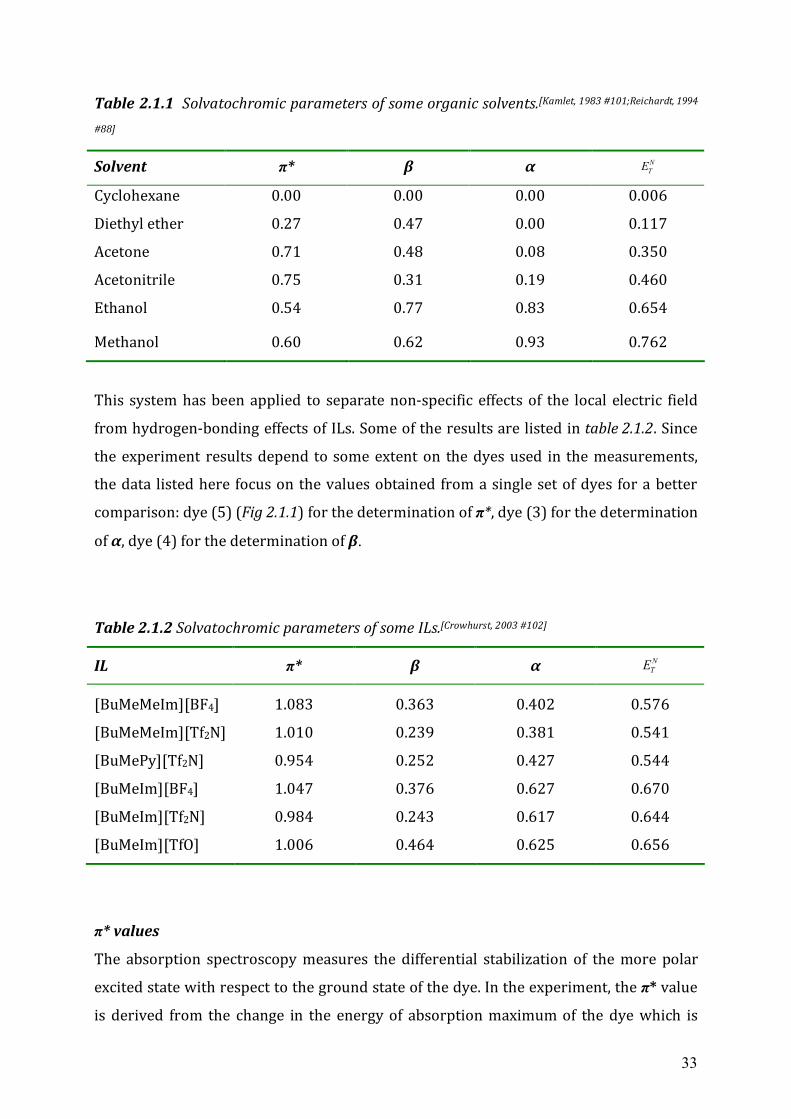
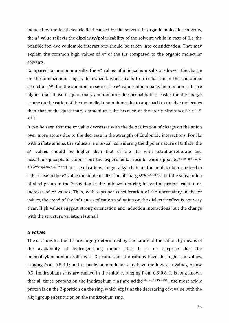
Table 2.1.1 Solvatochromic parameters of some organic solvents.[Kamlet, 1983 #101;Reichardt, 1994
#88]
Solvent π* β α NTE
Cyclohexane 0.00 0.00 0.00 0.006
Diethyl ether 0.27 0.47 0.00 0.117
Acetone 0.71 0.48 0.08 0.350
Acetonitrile 0.75 0.31 0.19 0.460
Ethanol 0.54 0.77 0.83 0.654
Methanol 0.60 0.62 0.93 0.762
This system has been applied to separate non-specific effects of the local electric field
from hydrogen-bonding effects of ILs. Some of the results are listed in table 2.1.2. Since
the experiment results depend to some extent on the dyes used in the measurements,
the data listed here focus on the values obtained from a single set of dyes for a better
comparison: dye (5) (Fig 2.1.1) for the determination of π*, dye (3) for the determination
of α, dye (4) for the determination of β.
Table 2.1.2 Solvatochromic parameters of some ILs.[Crowhurst, 2003 #102]
IL π* β α NTE
[BuMeMeIm][BF4]
[BuMeMeIm][Tf2N]
[BuMePy][Tf2N]
[BuMeIm][BF4]
[BuMeIm][Tf2N]
[BuMeIm][TfO]
1.083
1.010
0.954
1.047
0.984
1.006
0.363
0.239
0.252
0.376
0.243
0.464
0.402
0.381
0.427
0.627
0.617
0.625
0.576
0.541
0.544
0.670
0.644
0.656
π* values
The absorption spectroscopy measures the differential stabilization of the more polar
excited state with respect to the ground state of the dye. In the experiment, the π* value
is derived from the change in the energy of absorption maximum of the dye which is
34
induced by the local electric field caused by the solvent. In organic molecular solvents,
the π* value reflects the dipolarity/polarizability of the solvent; while in case of ILs, the
possible ion-dye coulombic interactions should be taken into consideration. That may
explain the common high values of π* of the ILs compared to the organic molecular
solvents.
Compared to ammonium salts, the π* values of imidazolium salts are lower; the charge
on the imidazolium ring is delocalized, which leads to a reduction in the coulombic
attraction. Within the ammonium series, the π* values of monoalkylammonium salts are
higher than those of quaternary ammonium salts; probably it is easier for the charge
centre on the cation of the monoalkylammonium salts to approach to the dye molecules
than that of the quaternary ammonium salts because of the steric hindrance.[Poole, 1989
#103]
It can be seen that the π* value decreases with the delocalization of charge on the anion
over more atoms due to the decrease in the strength of Coulombic interactions. For ILs
with triflate anions, the values are unusual; considering the dipolar nature of triflate, the
π* values should be higher than that of the ILs with tetrafluoroborate and
hexafluorophosphate anions, but the experimental results were opposite.[Crowhurst, 2003
#102;Weingärtner, 2009 #77] In case of cations, longer alkyl chain on the imidazolium ring lead to
a decrease in the π* value due to delocalization of charge[Peter, 2008 #9]; but the substitution
of alkyl group in the 2-position in the imidazolium ring instead of proton leads to an
increase of π* values. Thus, with a proper consideration of the uncertainty in the π*
values, the trend of the influences of cation and anion on the dielectric effect is not very
clear. High values suggest strong orientation and induction interactions, but the change
with the structure variation is small
α values
The α values for the ILs are largely determined by the nature of the cation, by means of
the availability of hydrogen-bong donor sites. It is no surprise that the
monoalkylammonium salts with 3 protons on the cations have the highest α values,
ranging from 0.8-1.1; and tetraalkylammonioum salts have the lowest α values, below
0.3; imidazolium salts are ranked in the middle, ranging from 0.3-0.8. It is long known
that all three protons on the imidazolium ring are acidic[Elaiwi, 1995 #104], the most acidic
proton is on the 2-position on the ring, which explains the decreasing of α value with the
alkyl group substitution on the imidazolium ring.
35
Although the α value relates mainly to the cation of the IL, the influence from the anion
can also be seen. With a common cation, such as [BuMeIm]+, there is small decrease of α
with the increasing hydrogen-bonding acceptor ability of the anion, e.g. from [BF4]- to
[[TfO]-. A probable explanation could be the competition between anion and probe dye
for the proton or the direct interactions between anion and dye[L.Crowhurst, 2003 #92].
β values
The β scale is a measure of the hydrogen bond basicity of the solvent. For ILs, the values
should be moderate and dominated by the nature of anions; the basicity increases with
decreasing strength of the conjugate acids. Since the conjugate acids are normally
strong, low values of the basicity of the anions are expected, compared to other solvents.
In fact, the experiment results show values of ILs close to other molecular solvents. The
data also indicate an influence of cations on the basicity of IL anions, but there is no clear
trend described due to the limited data.
2.1.2 The ET(30) and NTE scales
The ET(30) scale is based on the negatively solvatochromic pyridinium N-phenolate
betaine dye (3 in Fig.2.1.1) as probe molecule. It is defined as the molar electronic
transition energies (ET) of dissolved dye 3, measured in kilocalories per mole (kcal/mol)
at room temperature (25°C) and normal pressure (1 bar), according to the
eqn.(2.1.2)[Reichardt, 1994 #88]:
)(/28591~)108591.2(~)30( maxmax3
max nmNhcE AT (2.1.2)
where νmax is the frequency and λmax the wavelength of the maximum of the longest
wavelength, intramolecular charge-transfer π-π* absorption band of dye 3. The structure
of this dye was first published by Christian Reichardt in 1963[Dimroth, 1963 #105] with a
formula number of 30 added for distinction from similar dyes. It is called “Reichardt’s
dye”.
Due to the highly dipolar electronic ground state of μ = 15D and less dipolar electronic
excited state of μ = 6D, Reichardt’s dye has the longest wavelength absorption band,
36
which leads to the largest solvatochromic shifts of 375 nm, from λmax = 810 nm in
diphenyl ether (the least polar solvent in which the dye is sufficiently soluble) to λmax =
453 nm in water (the most polar solvent in which the dye is scarcely soluble).[Reichardt, 2005
#90] It can register the effect of solvent dipolarity and hydrogen bonding interactions
mainly with hydrogen bond donors. In 1983, the dimensionless normalized scale NTE
was introduced with NTE =1.00 for water and N
TE =0.00 for TMS as reference of the scale,
according to the eqn.2.1.3[Reichardt, 1983 #06]:
)()()()(
TMSEwaterETMSEsolventEE
TT
TTNT
(2.1.3)
The NTE scale has been applied to numbers of ILs[Poole, 1989 #103; Herfort, 1991 #107; L.Crowhurst, 2003
#92; Reichardt, 2005 #90], the values of some organic solvents and ILs are listed in table 2.2.1-
2.1.2. It can be seen that the values are more sensitive to the cations than to the anions;
since the positive charge of the dye is delocalized and sterically shielded, the
interactions with hydrogen bond acceptors are difficult to be detected. Similar to the π*
values, the monoalkylammonium salts have the highest value above 0.9,
tetraalkylammonium salts have the lowest below 0.5 and in between lie the imidazolium
salts. From the data of imidazolium salts with a proton in 2-position and those with
methyl group instead, the hydrogen bond donor properties of these cations are clearly
established.
2.1.3 Fluorescence spectroscopy
Fluorescence spectroscopy has also been applied to determine the polarity of ILs using
polycyclic aromatic hydrocarbon (PAH), such as pyrene (2, Fig 2.1.1). Unlike other
solvatochromic molecules, these PAHs do not exhibit spectral frequency shifts but a
variation in the ratio of emission band intensities that has been correlated with the
polarity of the PAH immediate environment. Pyrene is one of the most widely used
neutral fluorescence probes and its emission spectrum shows a significant enhancement
in the 0 - 0 vibronic band intensity in the presence of polar solvents. Based on this
37
emission response of an empirical relationship between solvent polarity and the pyrene
spontaneous emission band ratio has been established. This scale is defined as II/IIII
emission intensity ratio. Band I corresponds to a S1 (v = 0) → S0 (v = 0) transition and
band III corresponds to a S1 (v = 0) → S0 (v = 1) transition. The py scale was suggested to
be explained in terms of vibronic coupling. The dipolar nature of the solvent medium
determines the extent to which the formation of an induced dipole moment is formed by
vibrational distortion(s) of the nuclear coordinate. The increasing value of II/IIII
emission intensity ratio indicates the increasing solvent polarity. The important
intermolecular process that gives rise to the py scale is the interaction between the
solvent dipole and solute induced dipole.[Street, 1986 #108;Karpovich, 1995 #109]
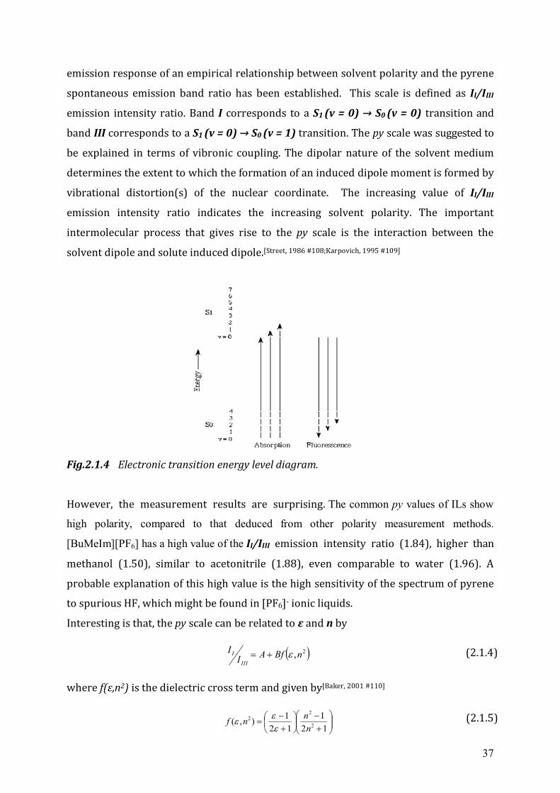
Fig.2.1.4 Electronic transition energy level diagram. However, the measurement results are surprising. The common py values of ILs show
high polarity, compared to that deduced from other polarity measurement methods.
[BuMeIm][PF6] has a high value of the II/IIII emission intensity ratio (1.84), higher than
methanol (1.50), similar to acetonitrile (1.88), even comparable to water (1.96). A
probable explanation of this high value is the high sensitivity of the spectrum of pyrene
to spurious HF, which might be found in [PF6]- ionic liquids.
Interesting is that, the py scale can be related to ε and n by 2,nBfAI
IIII
I (2.1.4)
where f(ε,n2) is the dielectric cross term and given by[Baker, 2001 #110]
121
121),( 2
22
nnnf
(2.1.5)
38
The spectrum shifts of another fluorescence probe PRODAN can also be related by .2 2
3 consthca
fSS GE
(2.1.6)
where h is Planck’s constant, c is the speed of light, a is the cavity radius swept out by
the PRODAN molecule, μE is the PRODAN’s excited-state dipole moment, μG is PRODAN’s
ground-state dipole moment, and ∆f is the solvent’s orientational polarizability, which is
given by[Baker, 2001 #110]
12
112
12
2
nnf
(2.1.7)
Based on these two probes, Baker et al. estimated ε ≈ 11.4 for [BuMeIm][PF6][Baker, 2001
#110], which is in good agreement with the data measured by dielectric spectroscopy.
2.2 Chromatographic Measurements
Another multi-parameter scale to describe the polarity of ILs is based on gas-liquid
chromatographic measurements using ILs as stationary phase. Separation in gas-liquid
chromatography is founded n the fact that the solutes interact to different extents with
the stationary liquid phase. The principal interactions that affect the solubility of a
solute in a liquid phase, e.g. retention, are dispersion, induction, orientation, and donor-
acceptor interactions, including hydrogen bonding[Poole, 1989#111]. To analyse the
contribution of the various intermolecular interactions to the singular observed value of
the retention parameter Abraham’s cavity model of solvation[Abraham, 1993 #112] has been
used[F.Poole, 1995 #113]. In this model, two Gibbs energy related steps for the transfer of a
solute from a gas state to the solvent are assumed: (1) creation of a cavity in the solvent
to accommodate the solute, which is endoergic due to the overcome of self-association of
the solvent; (2) incorporation of the solute in the cavity. The exergonic process is due to
the interaction of the solute molecule with the surrounding solvent molecules. The total
Gibbs energy change can be represented by the sum of individual Gibbs energy
contributions to the solvation process, as described by the eqn.(2.2.1):
162222 loglog LlbasrRcK HHH
L (2.2.1)
39
where c is a constant; KL, R2, π2H, α2H, β2H, and L16 are solvation parameters derived
from equilibrium measurements and refined by multiple linear regression analysis on
solvents of assumed characteristic properties: KL is the solute gas-liquid partition
coefficient, R2 is the solute excess molar refraction, π2H is the effective solute
dipolarity/polarizability parameter, α2H is the effective hydrogen-bond acidity, β2H is the
effective hydrogen bond basicity and L16 is the gas-liquid partition coefficient on
hexadecane at 25°C; r, s, a, b, l are solvent parameters: r is the ability of the solvent to
interact with solute through π- and n-electron pairs, s refers to the contribution of
solvents to the dipole-dipole and dipole-induced dipole interactions, a is the hydrogen
bond basicity of the solvent, b is the hydrogen bond acidity of the solvent, l incorporates
contributions from solvent cavity formation and dispersion interactions and indicates
how well the solvent will separate members of a homologous series. In table 2.2.1 lists
the characteristic solvent constants of some ILs.
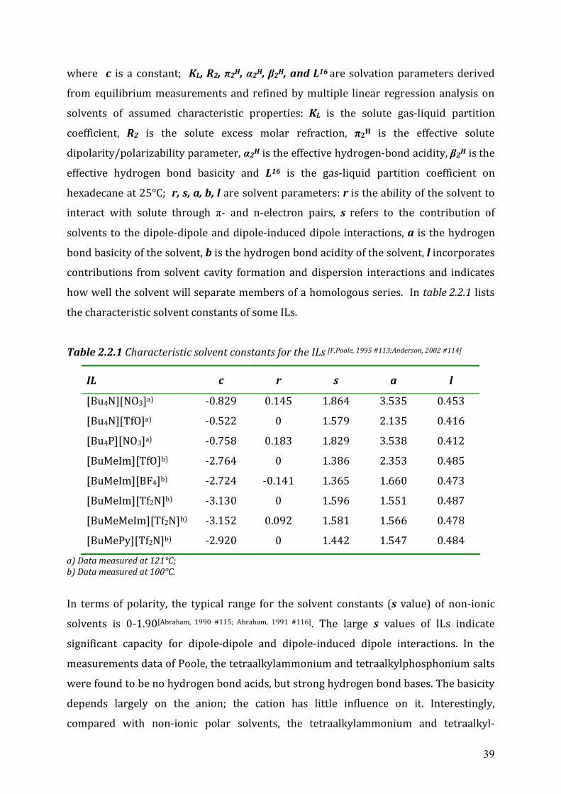
Table 2.2.1 Characteristic solvent constants for the ILs [F.Poole, 1995 #113;Anderson, 2002 #114]
IL c r s a l
[Bu4N][NO3]a) -0.829 0.145 1.864 3.535 0.453
[Bu4N][TfO]a) -0.522 0 1.579 2.135 0.416
[Bu4P][NO3]a) -0.758 0.183 1.829 3.538 0.412
[BuMeIm][TfO]b) -2.764 0 1.386 2.353 0.485
[BuMeIm][BF4]b) -2.724 -0.141 1.365 1.660 0.473
[BuMeIm][Tf2N]b) -3.130 0 1.596 1.551 0.487
[BuMeMeIm][Tf2N]b) -3.152 0.092 1.581 1.566 0.478
[BuMePy][Tf2N]b) -2.920 0 1.442 1.547 0.484
a) Data measured at 121°C; b) Data measured at 100°C.
In terms of polarity, the typical range for the solvent constants (s value) of non-ionic
solvents is 0-1.90[Abraham, 1990 #115; Abraham, 1991 #116]. The large s values of ILs indicate
significant capacity for dipole-dipole and dipole-induced dipole interactions. In the
measurements data of Poole, the tetraalkylammonium and tetraalkylphosphonium salts
were found to be no hydrogen bond acids, but strong hydrogen bond bases. The basicity
depends largely on the anion; the cation has little influence on it. Interestingly,
compared with non-ionic polar solvents, the tetraalkylammonium and tetraalkyl-
40
phosphonium salts with non-associating anions have surprisingly large l constants,
which is unusual among the polar solvents. Compared to ammonium based ILs,
imidazolium based ILs have relatively smaller s values and hydrogen bond basicity. The
dipolarity and the hydrogen bond basicity of ILs with the same cation and different
anions are quite different, while the changing of cation has little effect on them. Anions
have a clearly dominant influence on the dipolarity and hydrogen bond basicity.
2.3 Electron paramagnetic resonance spectroscopy Electron paramagnetic resonance spectroscopy (EPR) also called electron spin
resonance spectroscopy (ESR) has also been applied to assess the polarity of ILs. EPR is
used to investigate paramagnetic species, which have one or more unpaired electrons,
including organic and inorganic free radicals, triplet states or inorganic complexes with
a transition metal ion. EPR was first discovered by the Soviet physicist Yevgeny
Konstantinovich Zavoisky in 1944. The basic principles of EPR are very similar to the
NMR, except that it detects the signal from the excited electron spins instead of the
atomic nuclei spins. The limitation to paramagnetic species makes EPR to be a special
technique, since ordinary chemical solvents and matrices do not give rise to EPR spectra.
Every electron has a magnetic moment and spin quantum number s = 1/2, with
magnetic components ms = +1/2 and ms = -1/2. In the presence of an external magnetic
field, the electron's magnetic moment aligns itself either parallel (ms = -1/2) or
antiparallel (ms = +1/2) to the field, each alignment having a specific energy and the
difference between energy levels is 0BgE BE (Fig.2.3.1). The unpaired electron can
move between these two energy levels by absorbing or emitting corresponding energy,
so that the resonance takes place when the electromagnetic radiation of energy h
corresponds to the energy difference ∆E.
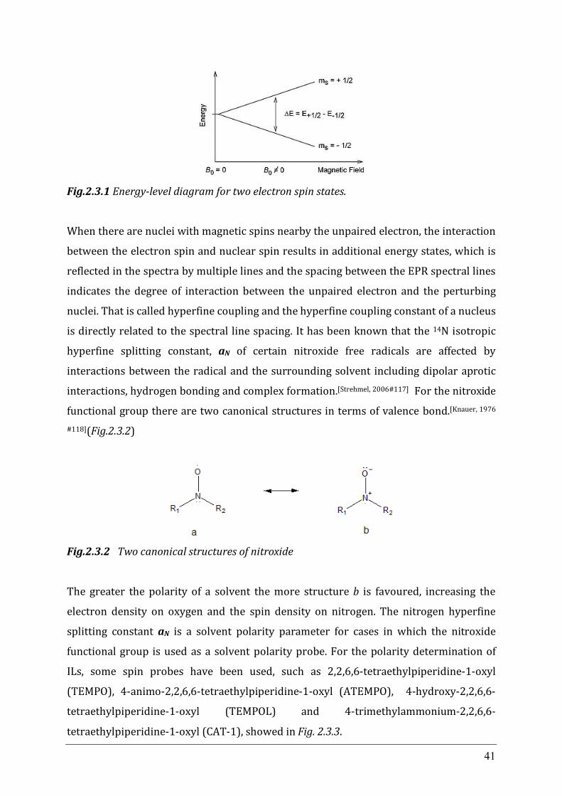
41
Fig.2.3.1 Energy-level diagram for two electron spin states.
When there are nuclei with magnetic spins nearby the unpaired electron, the interaction
between the electron spin and nuclear spin results in additional energy states, which is
reflected in the spectra by multiple lines and the spacing between the EPR spectral lines
indicates the degree of interaction between the unpaired electron and the perturbing
nuclei. That is called hyperfine coupling and the hyperfine coupling constant of a nucleus
is directly related to the spectral line spacing. It has been known that the 14N isotropic
hyperfine splitting constant, aN of certain nitroxide free radicals are affected by
interactions between the radical and the surrounding solvent including dipolar aprotic
interactions, hydrogen bonding and complex formation.[Strehmel, 2006#117] For the nitroxide
functional group there are two canonical structures in terms of valence bond.[Knauer, 1976
#118](Fig.2.3.2)
Fig.2.3.2 Two canonical structures of nitroxide
The greater the polarity of a solvent the more structure b is favoured, increasing the
electron density on oxygen and the spin density on nitrogen. The nitrogen hyperfine
splitting constant aN is a solvent polarity parameter for cases in which the nitroxide
functional group is used as a solvent polarity probe. For the polarity determination of
ILs, some spin probes have been used, such as 2,2,6,6-tetraethylpiperidine-1-oxyl
(TEMPO), 4-animo-2,2,6,6-tetraethylpiperidine-1-oxyl (ATEMPO), 4-hydroxy-2,2,6,6-
tetraethylpiperidine-1-oxyl (TEMPOL) and 4-trimethylammonium-2,2,6,6-
tetraethylpiperidine-1-oxyl (CAT-1), showed in Fig. 2.3.3.
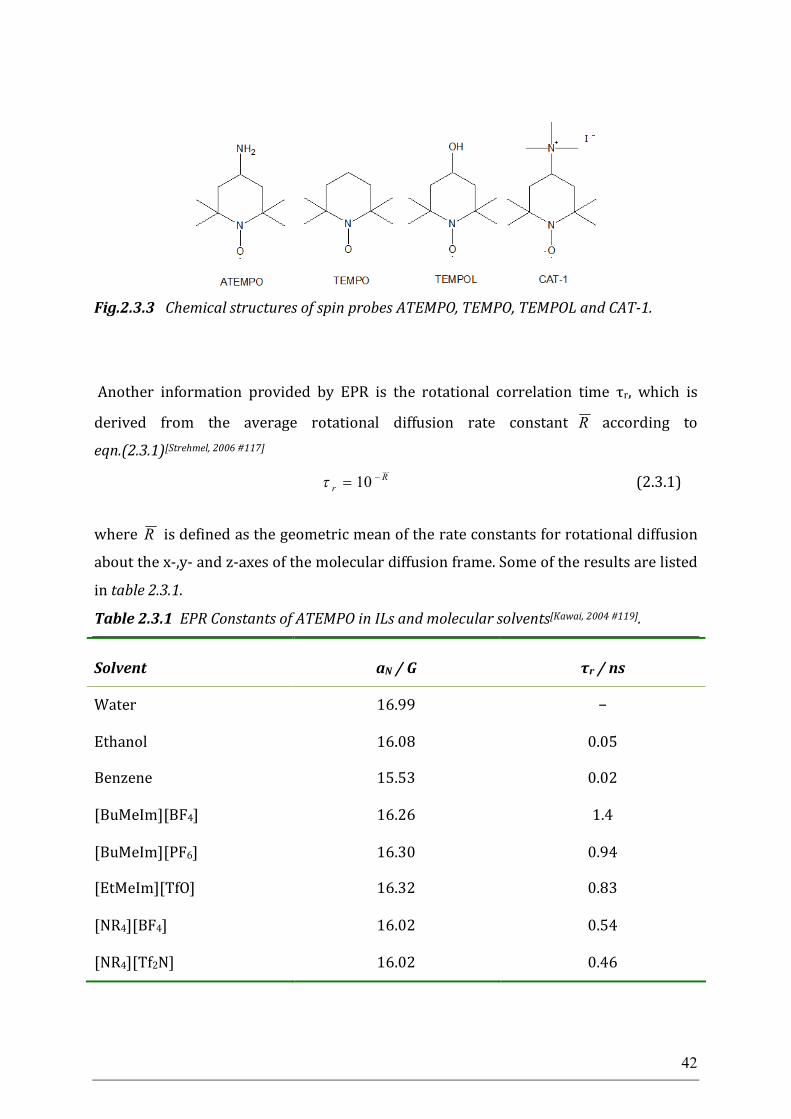
42
Fig.2.3.3 Chemical structures of spin probes ATEMPO, TEMPO, TEMPOL and CAT-1.
Another information provided by EPR is the rotational correlation time τr, which is
derived from the average rotational diffusion rate constant R according to
eqn.(2.3.1)[Strehmel, 2006 #117]
Rr
10 (2.3.1)
where R is defined as the geometric mean of the rate constants for rotational diffusion
about the x-,y- and z-axes of the molecular diffusion frame. Some of the results are listed
in table 2.3.1.
Table 2.3.1 EPR Constants of ATEMPO in ILs and molecular solvents[Kawai, 2004 #119].
Solvent aN / G τr / ns
Water 16.99 −
Ethanol 16.08 0.05
Benzene 15.53 0.02
[BuMeIm][BF4] 16.26 1.4
[BuMeIm][PF6] 16.30 0.94
[EtMeIm][TfO] 16.32 0.83
[NR4][BF4] 16.02 0.54
[NR4][Tf2N] 16.02 0.46
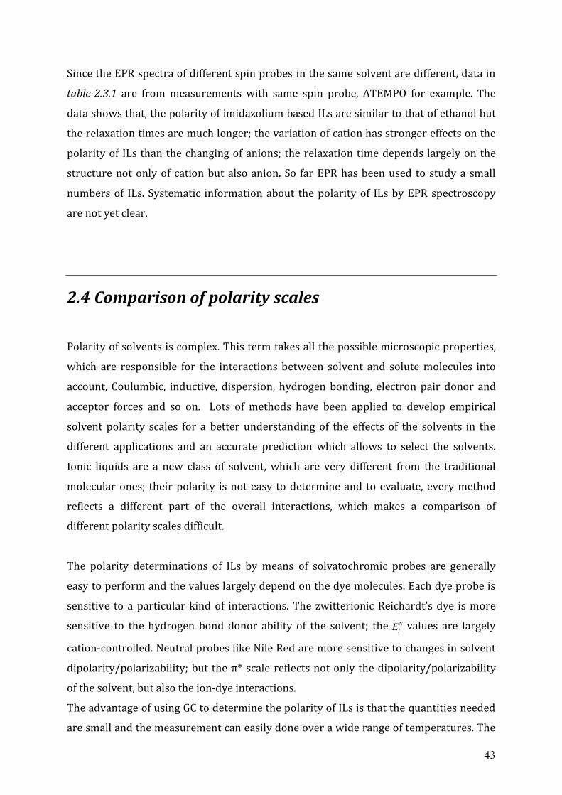
43
Since the EPR spectra of different spin probes in the same solvent are different, data in
table 2.3.1 are from measurements with same spin probe, ATEMPO for example. The
data shows that, the polarity of imidazolium based ILs are similar to that of ethanol but
the relaxation times are much longer; the variation of cation has stronger effects on the
polarity of ILs than the changing of anions; the relaxation time depends largely on the
structure not only of cation but also anion. So far EPR has been used to study a small
numbers of ILs. Systematic information about the polarity of ILs by EPR spectroscopy
are not yet clear.
2.4 Comparison of polarity scales
Polarity of solvents is complex. This term takes all the possible microscopic properties,
which are responsible for the interactions between solvent and solute molecules into
account, Coulumbic, inductive, dispersion, hydrogen bonding, electron pair donor and
acceptor forces and so on. Lots of methods have been applied to develop empirical
solvent polarity scales for a better understanding of the effects of the solvents in the
different applications and an accurate prediction which allows to select the solvents.
Ionic liquids are a new class of solvent, which are very different from the traditional
molecular ones; their polarity is not easy to determine and to evaluate, every method
reflects a different part of the overall interactions, which makes a comparison of
different polarity scales difficult.
The polarity determinations of ILs by means of solvatochromic probes are generally
easy to perform and the values largely depend on the dye molecules. Each dye probe is
sensitive to a particular kind of interactions. The zwitterionic Reichardt’s dye is more
sensitive to the hydrogen bond donor ability of the solvent; the NTE values are largely
cation-controlled. Neutral probes like Nile Red are more sensitive to changes in solvent
dipolarity/polarizability; but the π* scale reflects not only the dipolarity/polarizability
of the solvent, but also the ion-dye interactions.
The advantage of using GC to determine the polarity of ILs is that the quantities needed
are small and the measurement can easily done over a wide range of temperatures. The
44
polarity scale from GC measurements is also a multi-parameter scale. Similar to the π*
value, the high dipolar parameter s is probably due to the extra contribution from ion-
ion and ion-dipole interactions.
In both experiments, the hydrogen bond basicities of ILs are showed to be controlled by
anion. The agreement is worse for the hydrogen bond acidities. In GC measurements the
hydrogen bond acidities are largely affected by anion, while in Kamlet-Taft
measurements the cation plays an important role.
The py scale of the fluorescence spectroscopy is based on the effects from the polar
solvents on the radiative transition rate of the (0,0) band in fluorescence. The polar
solvents enhance the oscillator strength of symmetry-forbidden transitions through a
reduction of local symmetry[A.Winnik, 1985 #120]. The mechanism for that remains unclear,
which makes it difficult to interpret the results of the measurements.
EPR spectroscopy provides another polarity scale using spin probes. The results show
different trends of polarity for different probes; the hyperfine coupling constants of
TEMPO and TEMPOL dissolved in the ILs do not depend on the structure of the ILs,
while the results of CAT-1 strongly depend on structural variation of the ILs. Interesting
is that the values from the measurement with ATEMPO correlate very well with the
ET(30) scale.
Many of these polarity methods use probes molecules and the polarity scale depends to
a certain extent on the choice of the probe.[Strehmel, 2006 #121] Each scale maps a different
contribution; the choice of an appropriate polarity scale and probe depends on the
solute of interest and on the projected applications of ILs. Comparison of these scales
may not be very helpful to draw the whole picture of the polarity of ILs, but are helpful
to get a further understanding of the solvent-solute interactions.
45
Chapter 3 Dielectric Relaxation Theory The most common polarity scale relies on the static dielectric constant ε. In case of ILs,
the traditional standard methods are not available for the determination of dielectric
constants due to their intrinsic electrical conductance. However, this quantity can be
derived from microwave dielectric relaxation spectroscopy [Weingärtner, 2001 #76;Daguenet, 2006
#75;Schrodle, 2006 #74;Ingo Krossing, 2007 #48;Huang, 2008 #122;Weingärtner, 2009 #77].
Dielectric relaxation is a many particle phenomenon; it can be used as a suitable tool to
get insight into specific molecular interactions in polar liquids. Dielectric relaxation
parameters describe the behaviour of certain relaxing moieties, which generally consist
of a number of molecules correlated by short range interactions. The history of dielectric
theory can be traced back to the pioneering work of Faraday[Faraday, 1837#123] and
Maxwell[J.C.Maxwell, 1865 #124;J.C.Maxwell, 1868 #125] and later work by Clausius-Mossotti[R.Clausius,
1879 #126;P.F.Mossotti, 1847 #127], and Lorentz-Lorenz[L.Lorenz, 1880 #128;H.A.Lorentz, 1880 #129;H.A.Lorentz, 1952
#130]. The present interpretation of the dielectric parameters correlated to the molecular
structures is based upon the theory of Debye[P.Debye, 1929#131] and subsequent refinements.
In this chapter there will be a brief introduction of the dielectric relaxation theory
relevant to the measurement technique and current study.
3.1 Matter in the static electric field
3.1.1 The dielectric constant
The dielectric constant, also called “relative dielectric permittivity”, is a measure of the
ability of a material to store a charge from an applied electromagnetic field and then
transmit that energy. It can be defined as the ratio of the field strength in vacuum to that
in the material for the same distribution of charge. Consider a condenser consisting of
two parallel conducting plates, each of area A cm2, at a distance apart d cm. With a
potential difference V applied across the plates, which acquires charges +Q and –Q per
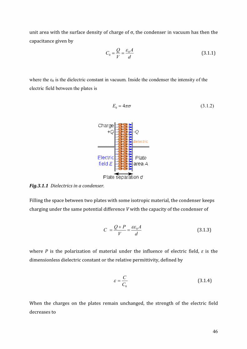
46
unit area with the surface density of charge of σ, the condenser in vacuum has then the
capacitance given by
dA
VQC 0
0
(3.1.1)
where the ε0 is the dielectric constant in vacuum. Inside the condenser the intensity of the
electric field between the plates is
40 E (3.1.2)
Fig.3.1.1 Dielectrics in a condenser.
Filling the space between two plates with some isotropic material, the condenser keeps
charging under the same potential difference V with the capacity of the condenser of
d
AV
PQC 0
(3.1.3)
where P is the polarization of material under the influence of electric field, ε is the
dimensionless dielectric constant or the relative permittivity, defined by
0C
C (3.1.4)
When the charges on the plates remain unchanged, the strength of the electric field
decreases to
47
4
E (3.1.5)
3.1.2 Polarizations
When placing a material between the plates of the condenser, the strength of the field
decreases, which could be effected by charging the surface of the dielectric opposite
each condenser plate with a charge of opposite sign to that on the plate. The surface
density of this charge is produced by an induced charge shift throughout the dielectric,
and is called polarization. It is given by
4
1 EP (3.1.6)
Different types of polarization can be classified. When placing a non-polar medium into
the condenser, under the influence of electric field two effects give rise to the
polarization: 1) the displacement of the electrons relative to the nucleus, called
electronic polarization; 2) the displacement of the atoms relative to one another, called
atomic polarization. When placing a polar medium into the condenser, another type of
polarization will occur in addition, called orientational polarization, which is due to
orientation of the molecular dipole in the field. A schematic representation of these
three types of polarization is shown in Fig.3.1.2.
The total polarization can be given by:
oraetotal PPPP (3.1.7)
where Pe is the electronic polarization, Pa the atomic polarization and Por the
orientational polarization; the Pe and Pa is due to distortion of the molecule by the field and
collectively called induced polarization Pind.. Under the electric field with the field
strength of E, the correlation between dielectric constant ε and the polarization P can be
given by:
EP stotal )1(0 EP sor )(0 EPind )1(0 (3.1.8)
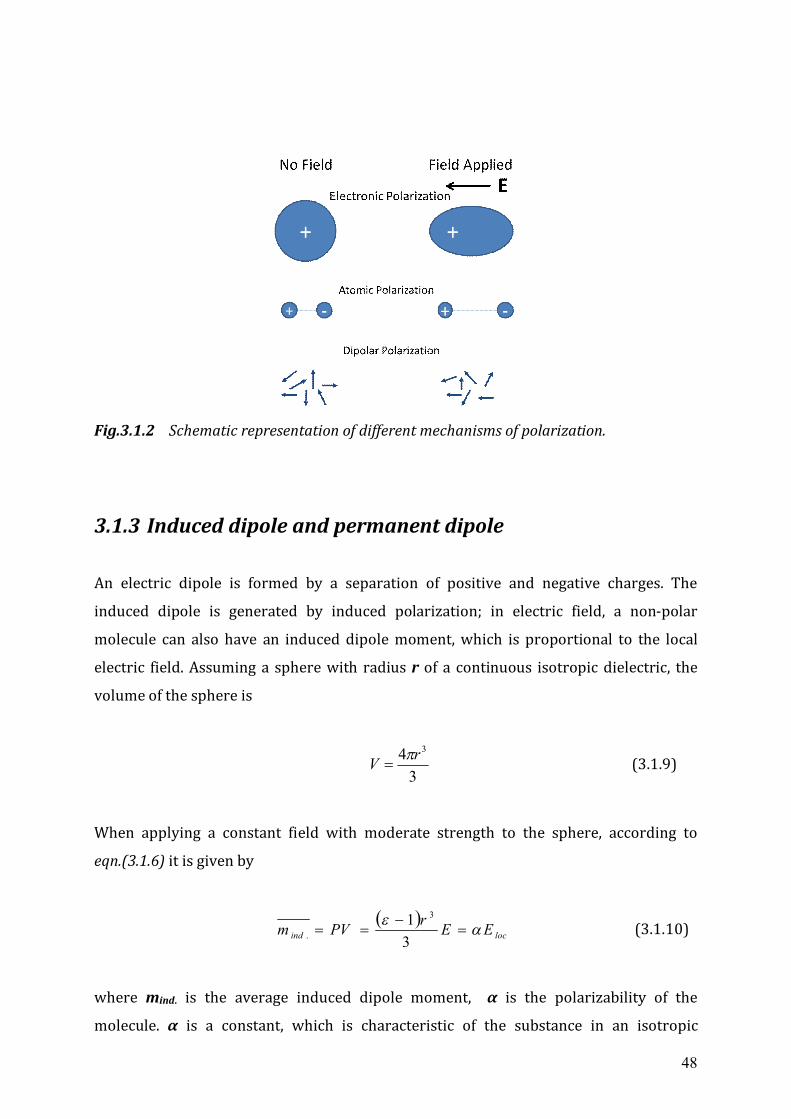
48
Fig.3.1.2 Schematic representation of different mechanisms of polarization.
3.1.3 Induced dipole and permanent dipole
An electric dipole is formed by a separation of positive and negative charges. The
induced dipole is generated by induced polarization; in electric field, a non-polar
molecule can also have an induced dipole moment, which is proportional to the local
electric field. Assuming a sphere with radius r of a continuous isotropic dielectric, the
volume of the sphere is
3
4 3rV (3.1.9)
When applying a constant field with moderate strength to the sphere, according to
eqn.(3.1.6) it is given by
locind EErPVm
31 3
. (3.1.10)
where mind. is the average induced dipole moment, α is the polarizability of the
molecule. α is a constant, which is characteristic of the substance in an isotropic
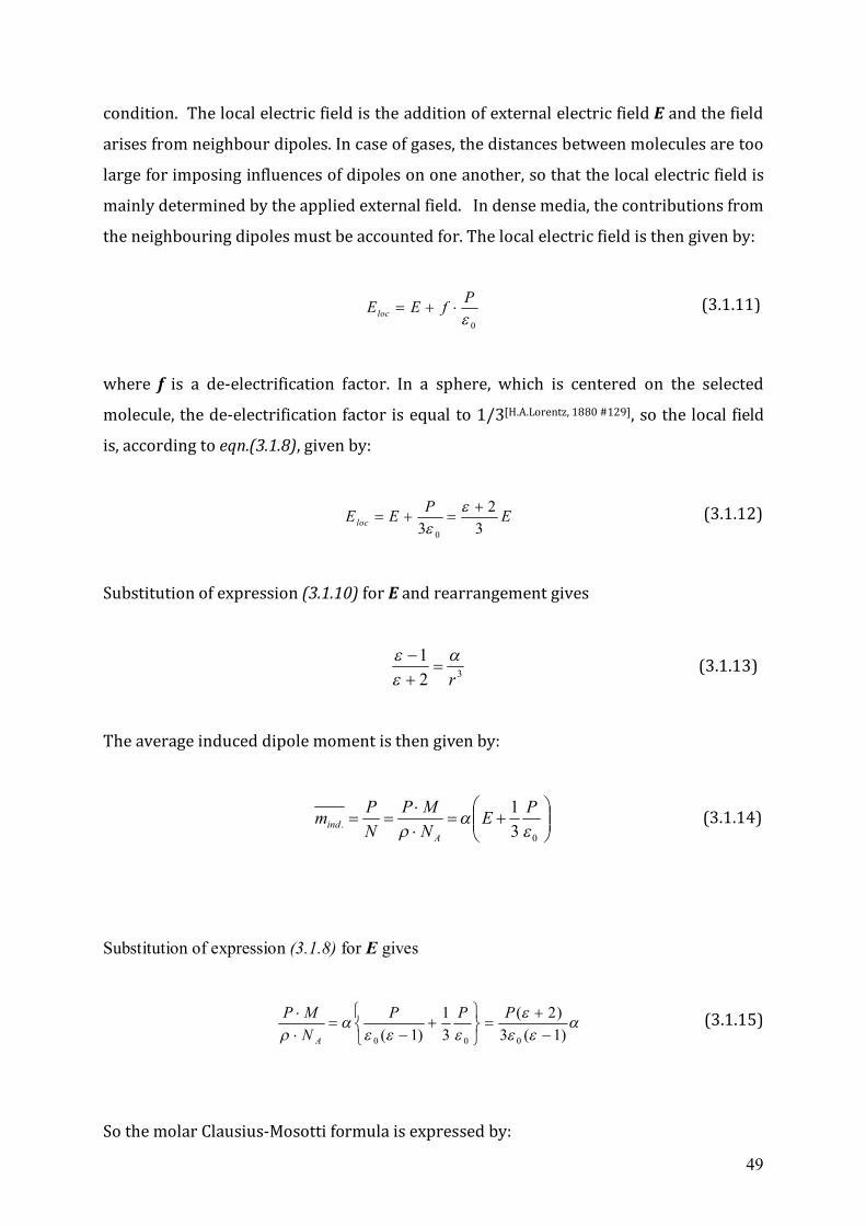
49
condition. The local electric field is the addition of external electric field E and the field
arises from neighbour dipoles. In case of gases, the distances between molecules are too
large for imposing influences of dipoles on one another, so that the local electric field is
mainly determined by the applied external field. In dense media, the contributions from
the neighbouring dipoles must be accounted for. The local electric field is then given by:
0
PfEEloc (3.1.11)
where f is a de-electrification factor. In a sphere, which is centered on the selected
molecule, the de-electrification factor is equal to 1/3[H.A.Lorentz, 1880 #129], so the local field
is, according to eqn.(3.1.8), given by:
EPEE loc 32
3 0
(3.1.12)
Substitution of expression (3.1.10) for E and rearrangement gives
321
r
(3.1.13)
The average induced dipole moment is then given by:
0
. 31
PENMP
NPm
Aind (3.1.14)
Substitution of expression (3.1.8) for E gives
)1(3)2(
31
)1( 000
PPPNMP
A
(3.1.15)
So the molar Clausius-Mosotti formula is expressed by:
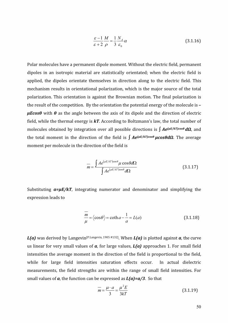
50
031
21 ANM
(3.1.16)
Polar molecules have a permanent dipole moment. Without the electric field, permanent
dipoles in an isotropic material are statistically orientated; when the electric field is
applied, the dipoles orientate themselves in direction along to the electric field. This
mechanism results in orientational polarization, which is the major source of the total
polarization. This orientation is against the Brownian motion. The final polarization is
the result of the competition. By the orientation the potential energy of the molecule is –
μEcosθ with θ as the angle between the axis of its dipole and the direction of electric
field, while the thermal energy is kT. According to Boltzmann’s law, the total number of
molecules obtained by integration over all possible directions is ∫ Ae(μE/kT)cosθ dΩ, and
the total moment in the direction of the field is ∫ Ae(μE/kT)cosθ μcosθdΩ. The average
moment per molecule in the direction of the field is
dAe
dAem
kTE
kTE
cos
cos cos (3.1.17)
Substituting a=μE/kT, integrating numerator and denominator and simplifying the
expression leads to
)(1cothcos aLa
am
(3.1.18)
L(a) was derived by Langevin[P.Langevin, 1905 #132]. When L(a) is plotted against a, the curve
us linear for very small values of a, for large values, L(a) approaches 1. For small field
intensities the average moment in the direction of the field is proportional to the field,
while for large field intensities saturation effects occur. In actual dielectric
measurements, the field strengths are within the range of small field intensities. For
small values of a, the function can be expressed as L(a)=a/3. So that
kT
Eam33
2
(3.1.19)
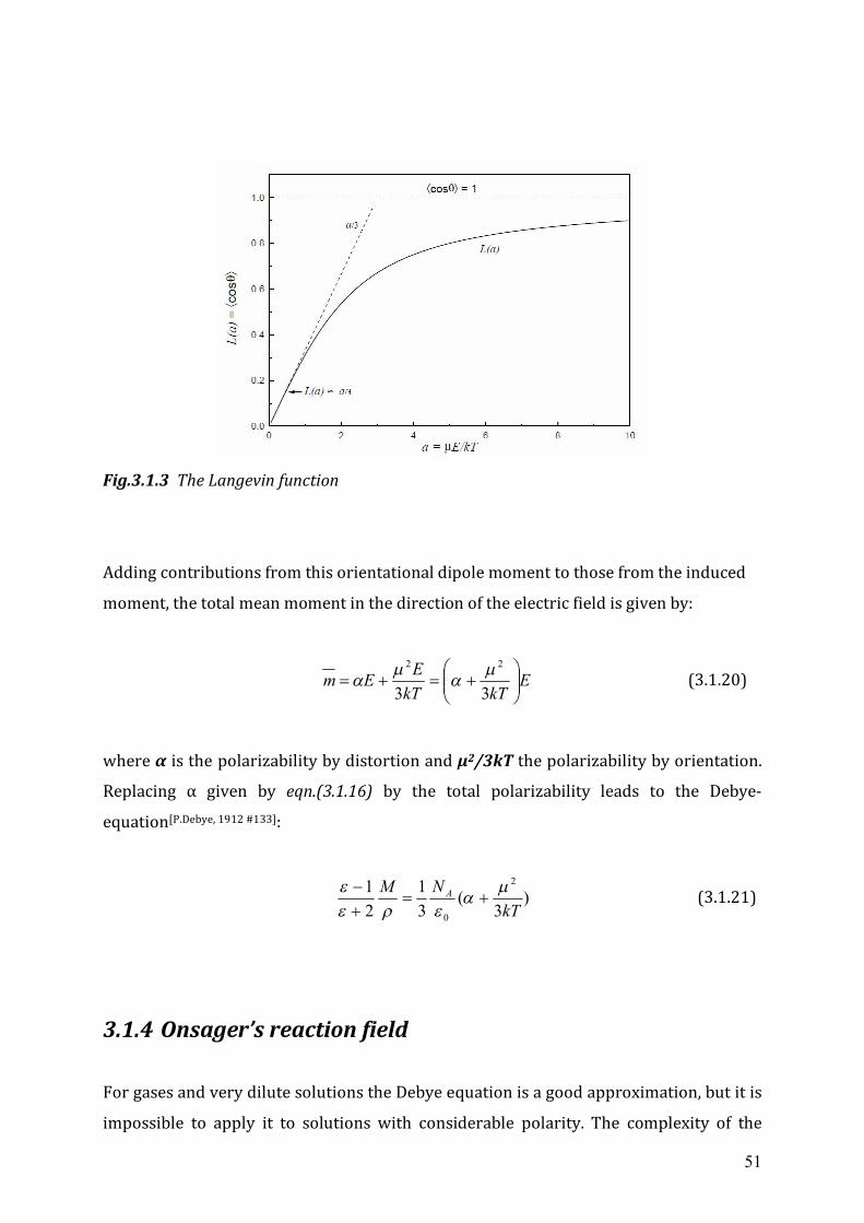
51
Fig.3.1.3 The Langevin function
Adding contributions from this orientational dipole moment to those from the induced
moment, the total mean moment in the direction of the electric field is given by:
EkTkT
EEm
33
22
(3.1.20)
where α is the polarizability by distortion and μ2/3kT the polarizability by orientation.
Replacing α given by eqn.(3.1.16) by the total polarizability leads to the Debye-
equation[P.Debye, 1912 #133]:
)3
(31
21 2
0 kTNM A
(3.1.21)
3.1.4 Onsager’s reaction field
For gases and very dilute solutions the Debye equation is a good approximation, but it is
impossible to apply it to solutions with considerable polarity. The complexity of the
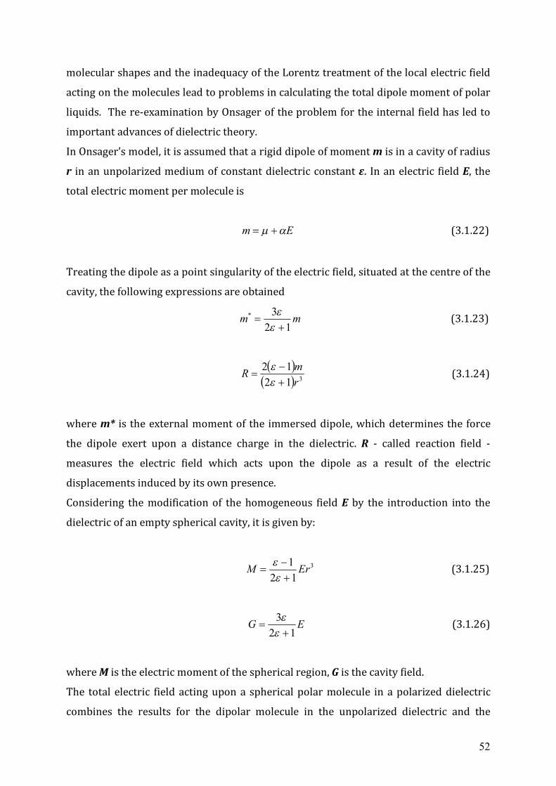
52
molecular shapes and the inadequacy of the Lorentz treatment of the local electric field
acting on the molecules lead to problems in calculating the total dipole moment of polar
liquids. The re-examination by Onsager of the problem for the internal field has led to
important advances of dielectric theory.
In Onsager’s model, it is assumed that a rigid dipole of moment m is in a cavity of radius
r in an unpolarized medium of constant dielectric constant ε. In an electric field E, the
total electric moment per molecule is
Em (3.1.22)
Treating the dipole as a point singularity of the electric field, situated at the centre of the
cavity, the following expressions are obtained
mm12
3*
(3.1.23)
312
12rmR
(3.1.24)
where m* is the external moment of the immersed dipole, which determines the force
the dipole exert upon a distance charge in the dielectric. R - called reaction field -
measures the electric field which acts upon the dipole as a result of the electric
displacements induced by its own presence.
Considering the modification of the homogeneous field E by the introduction into the
dielectric of an empty spherical cavity, it is given by:
3
121 ErM
(3.1.25)
EG12
3
(3.1.26)
where M is the electric moment of the spherical region, G is the cavity field.
The total electric field acting upon a spherical polar molecule in a polarized dielectric
combines the results for the dipolar molecule in the unpolarized dielectric and the
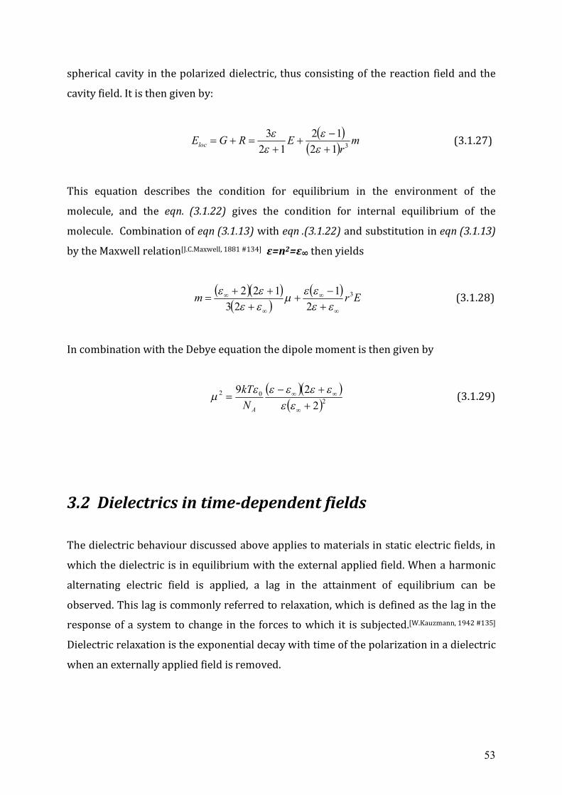
53
spherical cavity in the polarized dielectric, thus consisting of the reaction field and the
cavity field. It is then given by:
m
rERGEloc 312
1212
3
(3.1.27)
This equation describes the condition for equilibrium in the environment of the
molecule, and the eqn. (3.1.22) gives the condition for internal equilibrium of the
molecule. Combination of eqn (3.1.13) with eqn .(3.1.22) and substitution in eqn (3.1.13)
by the Maxwell relation[J.C.Maxwell, 1881 #134] ε=n2=ε∞ then yields
Erm 3
21
23122
(3.1.28)
In combination with the Debye equation the dipole moment is then given by
2
02
229
ANkT (3.1.29)
3.2 Dielectrics in time-dependent fields The dielectric behaviour discussed above applies to materials in static electric fields, in
which the dielectric is in equilibrium with the external applied field. When a harmonic
alternating electric field is applied, a lag in the attainment of equilibrium can be
observed. This lag is commonly referred to relaxation, which is defined as the lag in the
response of a system to change in the forces to which it is subjected.[W.Kauzmann, 1942 #135]
Dielectric relaxation is the exponential decay with time of the polarization in a dielectric
when an externally applied field is removed.
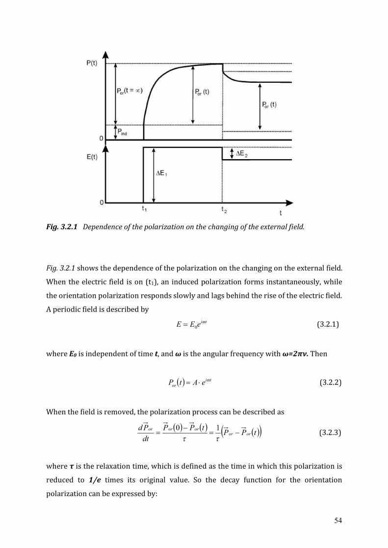
54
Fig. 3.2.1 Dependence of the polarization on the changing of the external field.
Fig. 3.2.1 shows the dependence of the polarization on the changing on the external field.
When the electric field is on (t1), an induced polarization forms instantaneously, while
the orientation polarization responds slowly and lags behind the rise of the electric field.
A periodic field is described by
tieEE 0 (3.2.1)
where E0 is independent of time t, and ω is the angular frequency with ω=2πν. Then
tior eAtP (3.2.2)
When the field is removed, the polarization process can be described as
tPPtPPdtPd
ororororor
10 (3.2.3)
where τ is the relaxation time, which is defined as the time in which this polarization is
reduced to 1/e times its original value. So the decay function for the orientation
polarization can be expressed by:
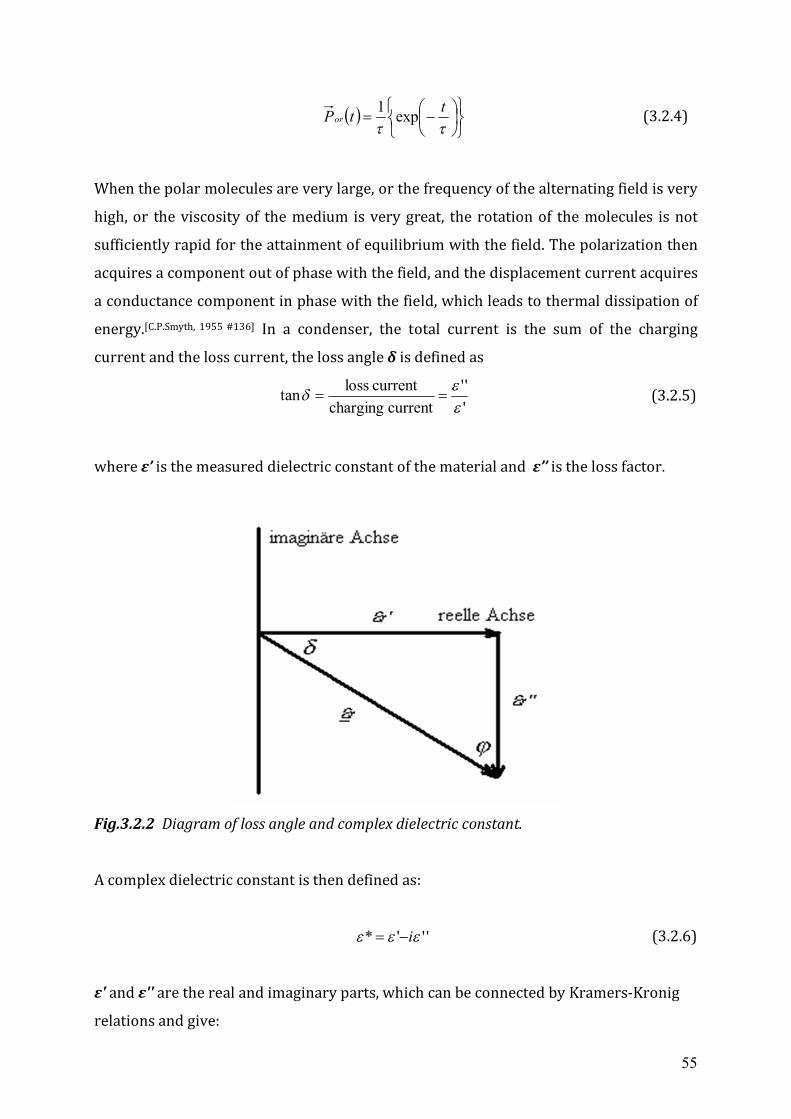
55
ttPor exp1 (3.2.4)
When the polar molecules are very large, or the frequency of the alternating field is very
high, or the viscosity of the medium is very great, the rotation of the molecules is not
sufficiently rapid for the attainment of equilibrium with the field. The polarization then
acquires a component out of phase with the field, and the displacement current acquires
a conductance component in phase with the field, which leads to thermal dissipation of
energy.[C.P.Smyth, 1955 #136] In a condenser, the total current is the sum of the charging
current and the loss current, the loss angle δ is defined as
'''
current chargingcurrent losstan
(3.2.5)
where ε’ is the measured dielectric constant of the material and ε’’ is the loss factor.
Fig.3.2.2 Diagram of loss angle and complex dielectric constant.
A complex dielectric constant is then defined as:
'''* i (3.2.6)
ε' and ε'' are the real and imaginary parts, which can be connected by Kramers-Kronig
relations and give:
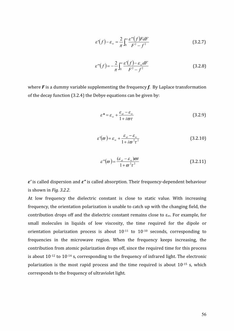
56
0 22''2'
fFFdFff
(3.2.7)
0 22
'2''fF
dFff
(3.2.8)
where F is a dummy variable supplementing the frequency f. By Laplace transformation
of the decay function (3.2.4) the Debye equations can be given by:
ist
1
* (3.2.9)
221'
ist
(3.2.10)
221)(''
tst (3.2.11)
ε’ is called dispersion and ε” is called absorption. Their frequency-dependent behaviour
is shown in Fig. 3.2.2.
At low frequency the dielectric constant is close to static value. With increasing
frequency, the orientation polarization is unable to catch up with the changing field, the
contribution drops off and the dielectric constant remains close to ε∞. For example, for
small molecules in liquids of low viscosity, the time required for the dipole or
orientation polarization process is about 10-11 to 10-10 seconds, corresponding to
frequencies in the microwave region. When the frequency keeps increasing, the
contribution from atomic polarization drops off, since the required time for this process
is about 10-12 to 10-14 s, corresponding to the frequency of infrared light. The electronic
polarization is the most rapid process and the time required is about 10-15 s, which
corresponds to the frequency of ultraviolet light.
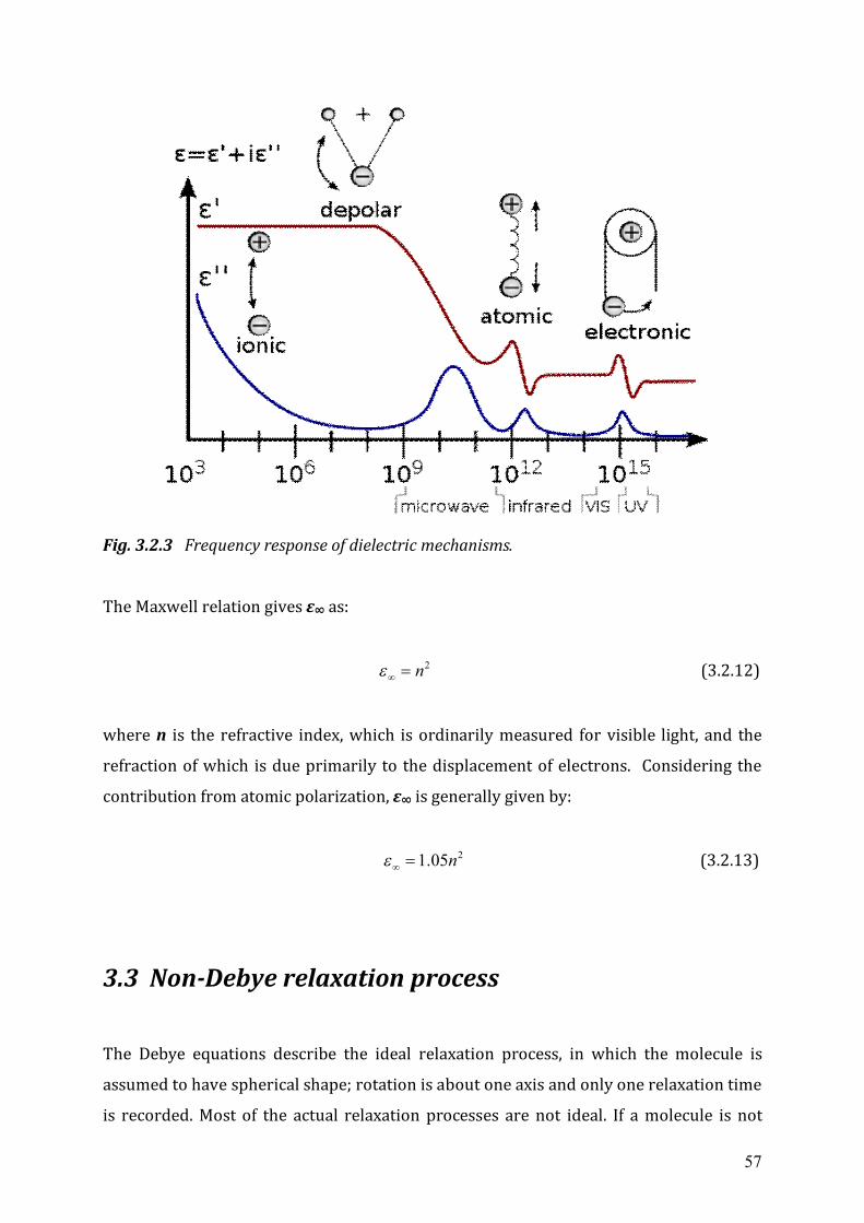
57
Fig. 3.2.3 Frequency response of dielectric mechanisms.
The Maxwell relation gives ε∞ as:
2n (3.2.12)
where n is the refractive index, which is ordinarily measured for visible light, and the
refraction of which is due primarily to the displacement of electrons. Considering the
contribution from atomic polarization, ε∞ is generally given by:
205.1 n (3.2.13)
3.3 Non-Debye relaxation process
The Debye equations describe the ideal relaxation process, in which the molecule is
assumed to have spherical shape; rotation is about one axis and only one relaxation time
is recorded. Most of the actual relaxation processes are not ideal. If a molecule is not
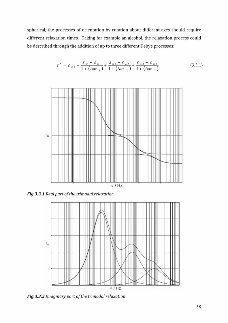
58
spherical, the processes of orientation by rotation about different axes should require
different relaxation times. Taking for example an alcohol, the relaxation process could
be described through the addition of up to three different Debye processes:
3
32
2
21
1
13 111
iii
st
(3.3.1)
Fig.3.3.1 Real part of the trimodal relaxation
Fig.3.3.2 Imaginary part of the trimodal relaxation
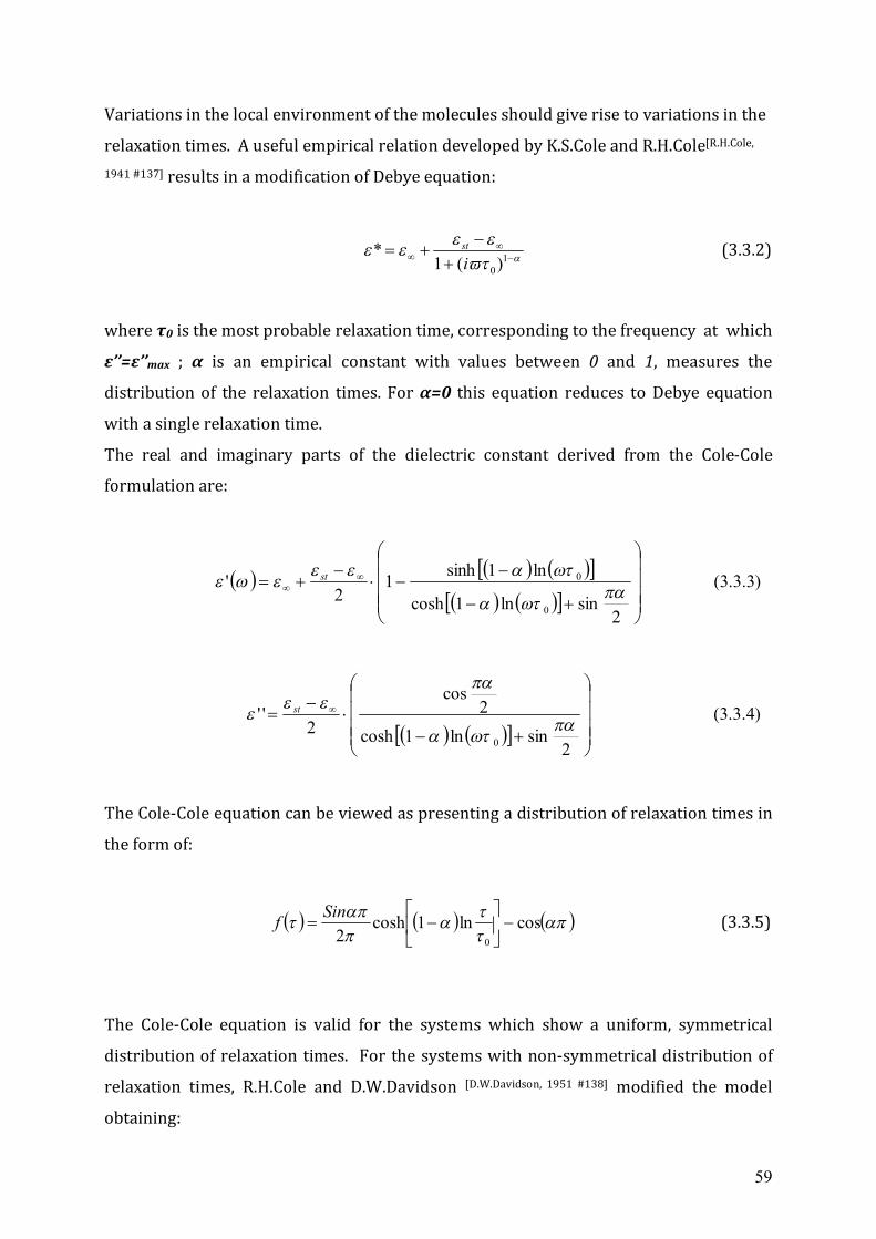
59
Variations in the local environment of the molecules should give rise to variations in the
relaxation times. A useful empirical relation developed by K.S.Cole and R.H.Cole[R.H.Cole,
1941 #137] results in a modification of Debye equation:
10)(1
*ist (3.3.2)
where τ0 is the most probable relaxation time, corresponding to the frequency at which
ε’’=ε’’max ; α is an empirical constant with values between 0 and 1, measures the
distribution of the relaxation times. For α=0 this equation reduces to Debye equation
with a single relaxation time.
The real and imaginary parts of the dielectric constant derived from the Cole-Cole
formulation are:
2sinln1cosh
ln1sinh12
'0
0
st (3.3.3)
2sinln1cosh
2cos
2''
0
st (3.3.4)
The Cole-Cole equation can be viewed as presenting a distribution of relaxation times in
the form of:
cosln1cosh
2 0
Sinf (3.3.5)
The Cole-Cole equation is valid for the systems which show a uniform, symmetrical
distribution of relaxation times. For the systems with non-symmetrical distribution of
relaxation times, R.H.Cole and D.W.Davidson [D.W.Davidson, 1951 #138] modified the model
obtaining:
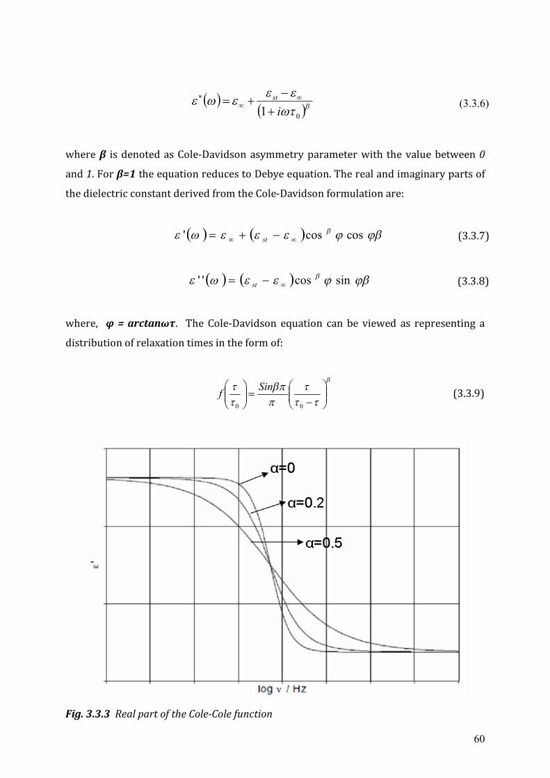
60
01 i
st
(3.3.6)
where β is denoted as Cole-Davidson asymmetry parameter with the value between 0
and 1. For β=1 the equation reduces to Debye equation. The real and imaginary parts of
the dielectric constant derived from the Cole-Davidson formulation are:
coscos' st (3.3.7)
sincos'' st (3.3.8)
where, φ = arctanωτ. The Cole-Davidson equation can be viewed as representing a
distribution of relaxation times in the form of:
00
Sinf (3.3.9)
Fig. 3.3.3 Real part of the Cole-Cole function
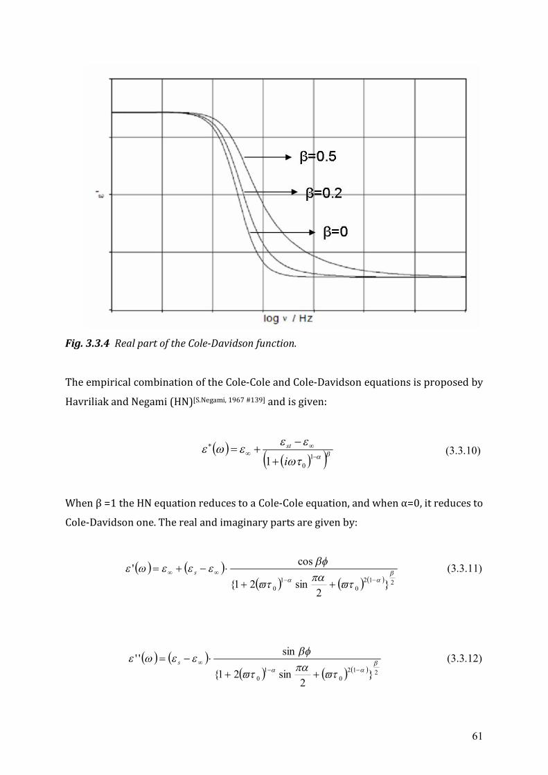
61
Fig. 3.3.4 Real part of the Cole-Davidson function.
The empirical combination of the Cole-Cole and Cole-Davidson equations is proposed by
Havriliak and Negami (HN)[S.Negami, 1967 #139] and is given:
101 i
st (3.3.10)
When β =1 the HN equation reduces to a Cole-Cole equation, and when α=0, it reduces to
Cole-Davidson one. The real and imaginary parts are given by:
212
01
0 }2
sin21{
cos'
s (3.3.11)
212
01
0 }2
sin21{
sin''
s (3.3.12)
62
where the can be expressed by:
2sin1
2cos
10
10
arctg (3.3.13)
63
Chapter 4 Experimental Setup The measurement of the dielectric properties of conducting materials like ionic liquids is
a difficult task. In non-glassy (low viscosity) ILs, the essential portion of the
reorientational dynamics of ions falls into the picosecond to nanosecond regime, which
corresponds to the microwave and radio frequency region (0.001GHz ~ 100GHz) of the
electromagnetic spectrum. Conventional techniques fail because the samples are largely
short-circuited by the high electrical conductance. Pilot studies show that, microwave
dielectric spectroscopy can be a suitable tool to measure the dielectric constant (ε’) and
loss factor (ε’’) of highly conducting ionic liquids and other ionic solvents[Weingärtner, 2001
#76; Weingärtner, 2009#77; Huang, 2008#122; Schrodle, 2006#74]. This method is based on coaxial
transmission line and wave guide techniques, which form basically a
reflection/transmission type spectroscopy and provide frequency coverage up to
several GHz. In the current study, reflection type of spectroscopy is used to measure the
dielectric properties of series of ILs. Depending on the frequency regime, it is divided
into a low-frequency part and high-frequency part; both will be introduced in this
chapter. Besides, a brief introduction of Karl-Fischer Coulometer, which is used to
determine the water content in ILs and in other solvents, will be inclusive in this
chapter.
4.1 High frequency dielectric spectrometer (50 MHz ~
20 GHz) For measurements of dielectric spectra at high frequency, a reflection dielectric
spectrometer with open-ended coaxial probe technique is employed.
4.1.1 Open-ended coaxial probe technique
A typical coaxial probe system consists of a vector network analyzer, a coaxial probe and
an external computer. This technique represents a coaxial line equipped with a tip that
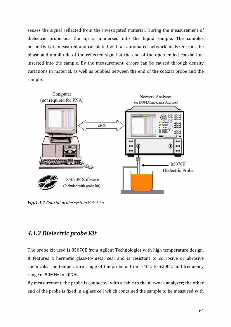
64
senses the signal reflected from the investigated material. During the measurement of
dielectric properties the tip is immersed into the liquid sample. The complex
permittivity is measured and calculated with an automated network analyzer from the
phase and amplitude of the reflected signal at the end of the open-ended coaxial line
inserted into the sample. By the measurement, errors can be caused through density
variations in material, as well as bubbles between the end of the coaxial probe and the
sample.
Fig.4.1.1 Coaxial probe system.[2004 #140]
4.1.2 Dielectric probe Kit
The probe kit used is 85070E from Agilent Technologies with high temperature design.
It features a hermetic glass-to-metal seal and is resistant to corrosive or abrasive
chemicals. The temperature range of the probe is from –40 ̊C to +200 ̊C and frequency
range of 50MHz to 20GHz.
By measurement, the probe is connected with a cable to the network analyzer; the other
end of the probe is fixed in a glass cell which contained the sample to be measured with
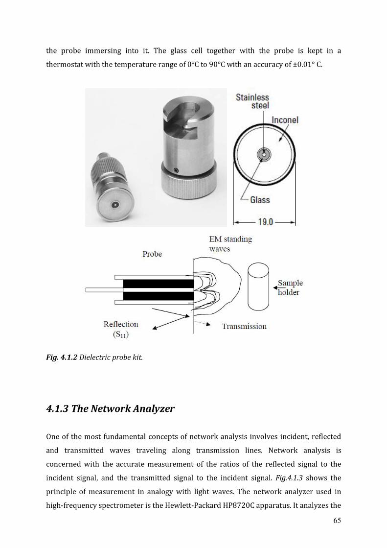
65
the probe immersing into it. The glass cell together with the probe is kept in a
thermostat with the temperature range of 0°C to 90°C with an accuracy of ±0.01° C.
Fig. 4.1.2 Dielectric probe kit.
4.1.3 The Network Analyzer
One of the most fundamental concepts of network analysis involves incident, reflected
and transmitted waves traveling along transmission lines. Network analysis is
concerned with the accurate measurement of the ratios of the reflected signal to the
incident signal, and the transmitted signal to the incident signal. Fig.4.1.3 shows the
principle of measurement in analogy with light waves. The network analyzer used in
high-frequency spectrometer is the Hewlett-Packard HP8720C apparatus. It analyzes the
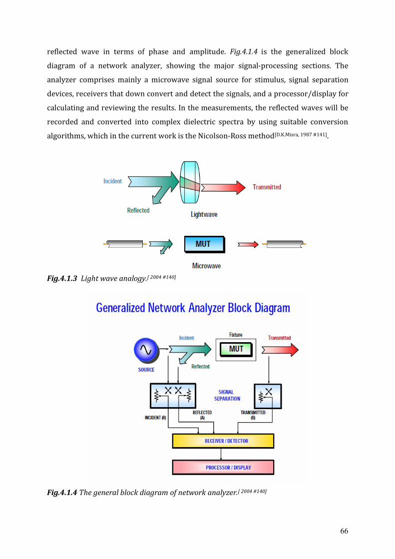
66
reflected wave in terms of phase and amplitude. Fig.4.1.4 is the generalized block
diagram of a network analyzer, showing the major signal-processing sections. The
analyzer comprises mainly a microwave signal source for stimulus, signal separation
devices, receivers that down convert and detect the signals, and a processor/display for
calculating and reviewing the results. In the measurements, the reflected waves will be
recorded and converted into complex dielectric spectra by using suitable conversion
algorithms, which in the current work is the Nicolson-Ross method[D.K.Misra, 1987 #141].
Fig.4.1.3 Light wave analogy.[ 2004 #140]
Fig.4.1.4 The general block diagram of network analyzer.[ 2004 #140]
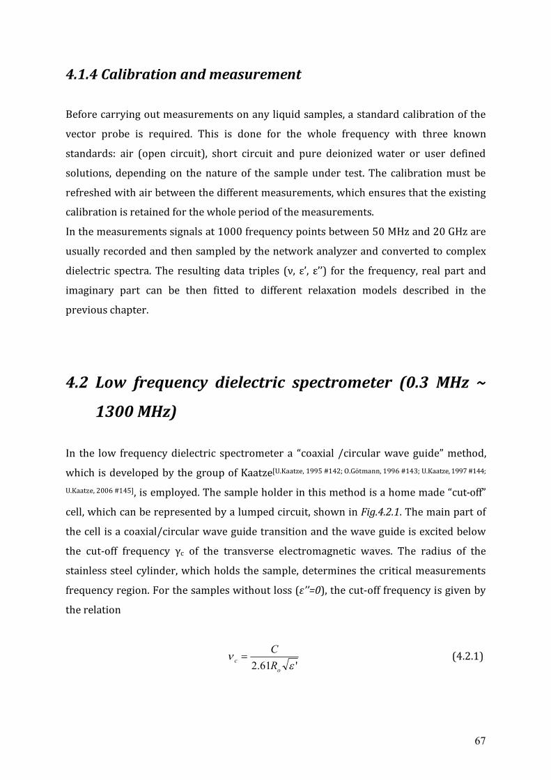
67
4.1.4 Calibration and measurement
Before carrying out measurements on any liquid samples, a standard calibration of the
vector probe is required. This is done for the whole frequency with three known
standards: air (open circuit), short circuit and pure deionized water or user defined
solutions, depending on the nature of the sample under test. The calibration must be
refreshed with air between the different measurements, which ensures that the existing
calibration is retained for the whole period of the measurements.
In the measurements signals at 1000 frequency points between 50 MHz and 20 GHz are
usually recorded and then sampled by the network analyzer and converted to complex
dielectric spectra. The resulting data triples (ν, ε’, ε’’) for the frequency, real part and
imaginary part can be then fitted to different relaxation models described in the
previous chapter.
4.2 Low frequency dielectric spectrometer (0.3 MHz ~
1300 MHz) In the low frequency dielectric spectrometer a “coaxial /circular wave guide” method,
which is developed by the group of Kaatze[U.Kaatze, 1995 #142; O.Götmann, 1996 #143; U.Kaatze, 1997 #144;
U.Kaatze, 2006 #145], is employed. The sample holder in this method is a home made “cut-off”
cell, which can be represented by a lumped circuit, shown in Fig.4.2.1. The main part of
the cell is a coaxial/circular wave guide transition and the wave guide is excited below
the cut-off frequency γc of the transverse electromagnetic waves. The radius of the
stainless steel cylinder, which holds the sample, determines the critical measurements
frequency region. For the samples without loss (ε’’=0), the cut-off frequency is given by
the relation
'61.2
o
c RC
(4.2.1)
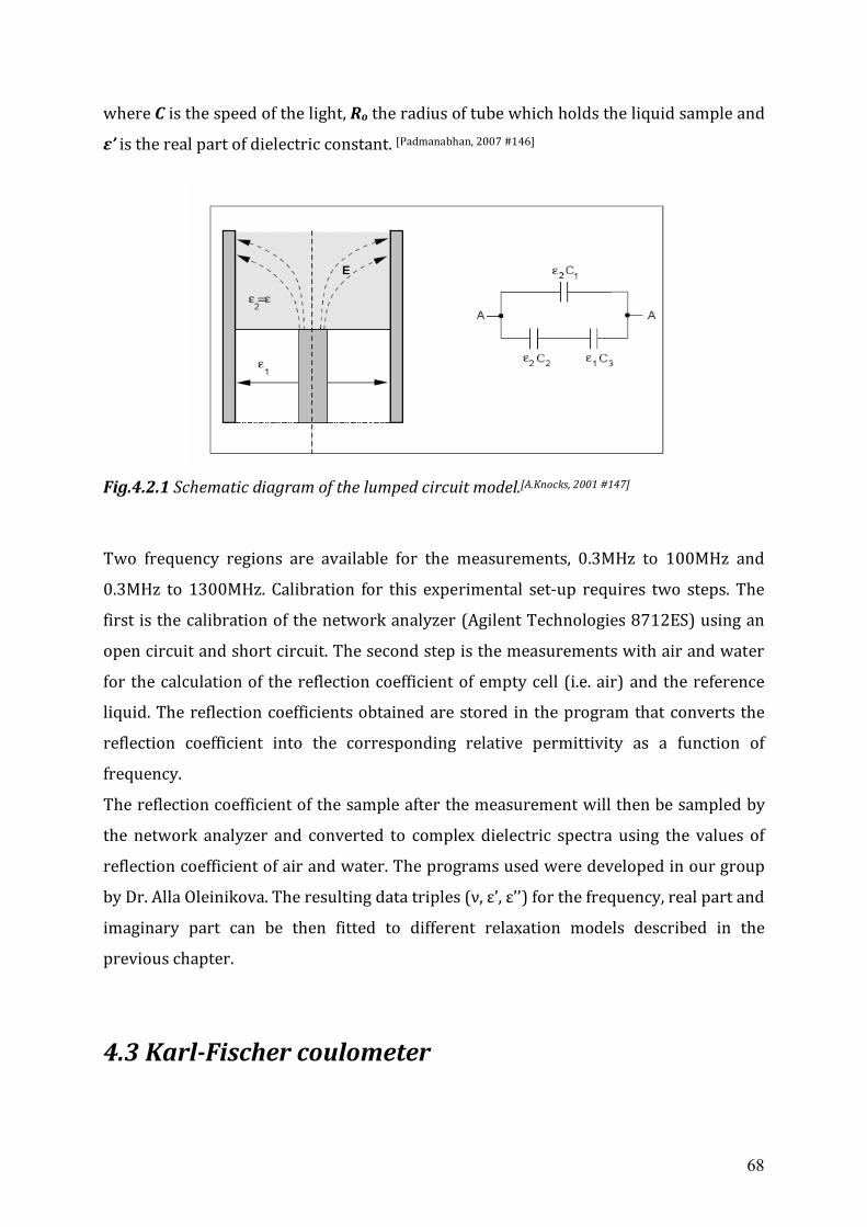
68
where C is the speed of the light, Ro the radius of tube which holds the liquid sample and
ε’ is the real part of dielectric constant. [Padmanabhan, 2007 #146]
Fig.4.2.1 Schematic diagram of the lumped circuit model.[A.Knocks, 2001 #147]
Two frequency regions are available for the measurements, 0.3MHz to 100MHz and
0.3MHz to 1300MHz. Calibration for this experimental set-up requires two steps. The
first is the calibration of the network analyzer (Agilent Technologies 8712ES) using an
open circuit and short circuit. The second step is the measurements with air and water
for the calculation of the reflection coefficient of empty cell (i.e. air) and the reference
liquid. The reflection coefficients obtained are stored in the program that converts the
reflection coefficient into the corresponding relative permittivity as a function of
frequency.
The reflection coefficient of the sample after the measurement will then be sampled by
the network analyzer and converted to complex dielectric spectra using the values of
reflection coefficient of air and water. The programs used were developed in our group
by Dr. Alla Oleinikova. The resulting data triples (ν, ε’, ε’’) for the frequency, real part and
imaginary part can be then fitted to different relaxation models described in the
previous chapter.
4.3 Karl-Fischer coulometer
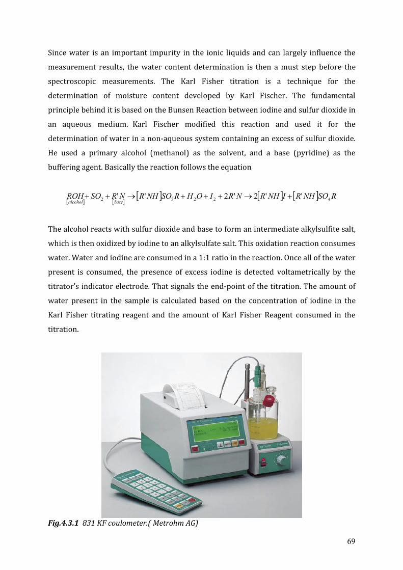
69
Since water is an important impurity in the ionic liquids and can largely influence the
measurement results, the water content determination is then a must step before the
spectroscopic measurements. The Karl Fisher titration is a technique for the
determination of moisture content developed by Karl Fischer. The fundamental
principle behind it is based on the Bunsen Reaction between iodine and sulfur dioxide in
an aqueous medium. Karl Fischer modified this reaction and used it for the
determination of water in a non-aqueous system containing an excess of sulfur dioxide.
He used a primary alcohol (methanol) as the solvent, and a base (pyridine) as the
buffering agent. Basically the reaction follows the equation
RSONHRINHRNRIOHRSONHRNRSOROH
basealcohol 42232 ''2'2''
The alcohol reacts with sulfur dioxide and base to form an intermediate alkylsulfite salt,
which is then oxidized by iodine to an alkylsulfate salt. This oxidation reaction consumes
water. Water and iodine are consumed in a 1:1 ratio in the reaction. Once all of the water
present is consumed, the presence of excess iodine is detected voltametrically by the
titrator’s indicator electrode. That signals the end-point of the titration. The amount of
water present in the sample is calculated based on the concentration of iodine in the
Karl Fisher titrating reagent and the amount of Karl Fisher Reagent consumed in the
titration.
Fig.4.3.1 831 KF coulometer.( Metrohm AG)
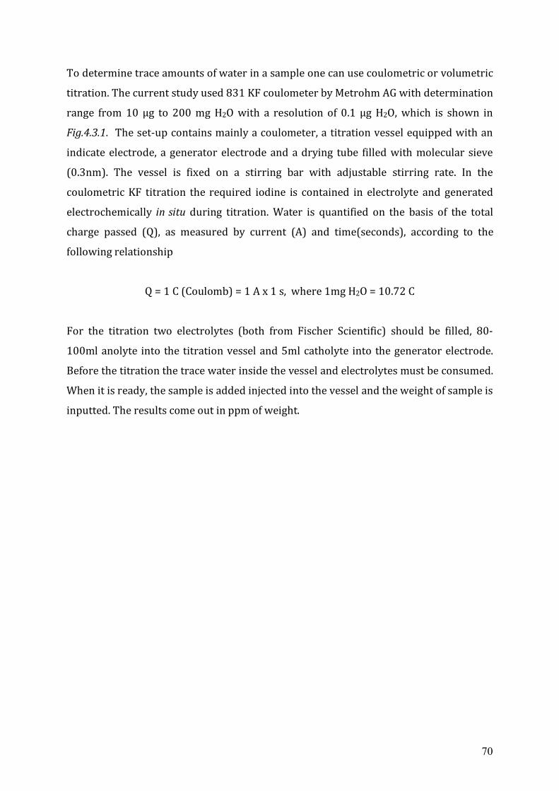
70
To determine trace amounts of water in a sample one can use coulometric or volumetric
titration. The current study used 831 KF coulometer by Metrohm AG with determination
range from 10 μg to 200 mg H2O with a resolution of 0.1 μg H2O, which is shown in
Fig.4.3.1. The set-up contains mainly a coulometer, a titration vessel equipped with an
indicate electrode, a generator electrode and a drying tube filled with molecular sieve
(0.3nm). The vessel is fixed on a stirring bar with adjustable stirring rate. In the
coulometric KF titration the required iodine is contained in electrolyte and generated
electrochemically in situ during titration. Water is quantified on the basis of the total
charge passed (Q), as measured by current (A) and time(seconds), according to the
following relationship
Q = 1 C (Coulomb) = 1 A x 1 s, where 1mg H2O = 10.72 C
For the titration two electrolytes (both from Fischer Scientific) should be filled, 80-
100ml anolyte into the titration vessel and 5ml catholyte into the generator electrode.
Before the titration the trace water inside the vessel and electrolytes must be consumed.
When it is ready, the sample is added injected into the vessel and the weight of sample is
inputted. The results come out in ppm of weight.
71
Chapter 5 Microwave Dielectric Dpectroscopy of Ionic Liquids
As neoteric materials and “green” solvents in chemical technology, ionic liquids are
receiving more and more attention. By using of ILs, a significant barrier is the absence of
understanding how the structure of ILs affects its physical properties and solvent
strength. The latter can be simply indicated by polarity and polarizability. Previous
work showed that dielectric relaxation spectroscopy can be used to determine the
solvent strength of ILs. In this chapter, the interpretation of the dielectric spectra of ILs
will be introduced as well as some experiment details, and the measurement results of
neat ILs will be discussed.
5.1 Microwave dielectric spectrum In microwave frequency range, the possible contributions to the complex dielectric
function Σ*(ν) originate from different processes: (a) microscopic fluctuations of
molecular dipoles (rotational contributions); (b) the propagation of mobile charge
carriers (translational contributions); (c) the separation of charges at interfaces
(Maxwell-Wagner polarization).[F.Kremer, 2002 #148] Ionic liquids are charged systems, the
contribution from rotation and translation can not be separated experimentally. The
complex dielectric function can be expressed either by the complex dielectric
permittivity or by complex dielectric conductivity. At non-zero frequency the
permittivity and conductivity are coupled, while at zero frequency are decoupled and
turn to be static dielectric constant and direct current conductivity. The latter one is
independently measurable, the complex dielectric function can be then expressed by
0
*
2'''
ii (5.1.1)

72
where σ is dc conductivity; the last term is a diverging low-frequency response of
imaginary part, called “ohmic loss”. The complex dielectric permittivity is expressed
by[Böttcher, 1972 #149; Böttcher, 1978 #150]
0
*
2''''''
iii (5.1.2)
where ε∞ is the high frequency limit of the real part. The key interest focus on the
relaxational terms of ∆ε’(ν) and ∆ε’’(ν). It is shown in the dielectric spectrum, with
increasing frequency, the real part ε’(ν) decreases step-like whereas the imaginary part
ε’’(ν) exhibits a maximum (Fig.5.1.1). The essential quantities which characterize the
dielectric relaxation process can be extracted from this behavior.
Fig.5.1.1 Frequency-dependent dielectric absorption.
Fig.5.1.2 shows a dielectric spectrum of [EtMeIm][Tf2N] as example, ε’(ν) is the
dielectric dispersion, ε’’(ν) is the dielectric loss with ohmic loss and ∆ε’’(ν) is corrected
imaginary part with ohmic loss being cut off. Static dielectric constant εs is defined as the
zero-frequency limit of the real part and can be extrapolated
'lim0
s (5.1.3)
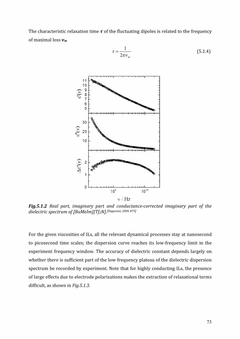
73
The characteristic relaxation time τ of the fluctuating dipoles is related to the frequency
of maximal loss νm
m
2
1 (5.1.4)
Fig.5.1.2 Real part, imaginary part and conductance-corrected imaginary part of the dielectric spectrum of [BuMeIm][Tf2N].[Daguenet, 2006 #75]
For the given viscosities of ILs, all the relevant dynamical processes stay at nanosecond
to picosecond time scales; the dispersion curve reaches its low-frequency limit in the
experiment frequency window. The accuracy of dielectric constant depends largely on
whether there is sufficient part of the low frequency plateau of the dielectric dispersion
spectrum be recorded by experiment. Note that for highly conducting ILs, the presence
of large effects due to electrode polarizations makes the extraction of relaxational terms
difficult, as shown in Fig.5.1.3.
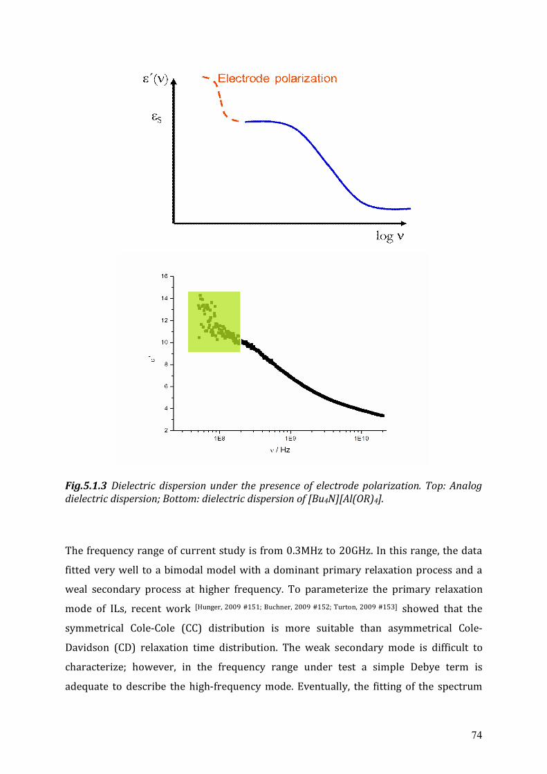
74
Fig.5.1.3 Dielectric dispersion under the presence of electrode polarization. Top: Analog dielectric dispersion; Bottom: dielectric dispersion of [Bu4N][Al(OR)4].
The frequency range of current study is from 0.3MHz to 20GHz. In this range, the data
fitted very well to a bimodal model with a dominant primary relaxation process and a
weal secondary process at higher frequency. To parameterize the primary relaxation
mode of ILs, recent work [Hunger, 2009 #151; Buchner, 2009 #152; Turton, 2009 #153] showed that the
symmetrical Cole-Cole (CC) distribution is more suitable than asymmetrical Cole-
Davidson (CD) relaxation time distribution. The weak secondary mode is difficult to
characterize; however, in the frequency range under test a simple Debye term is
adequate to describe the high-frequency mode. Eventually, the fitting of the spectrum
75
yielded terms from a combination of two processes. In this work, for all ILs the overall
fitting equation is the combination of a Cole-Cole function plus a Debye function given by
D
D
CC
CC
iS
iS
2121
)(* 1
(5.1.5)
221
2sin2ln1cosh
2ln1sinh12
'D
D
CC
CCCC SS
(5.1.6)
221
2sin2ln1cosh
2cos
2''
D
DD
CC
CC SS
(5.1.7)
For a spectrum describable by equation above, the static dielectric constant is given by
the sum of the amplitudes, εs = ε∞ + SCC + SD.
5.2 Dielectric relaxation measurements of aprotic ionic
liquids
Ionic liquids can be divided into two subsets, aprotic ILs and protic ILs. Previous
research work on ILs mainly focused on aprotic ones. In this section, the dielectric
behavior of series of aprotic ILs measured will be discussed. To get a comprehensive
understanding as far as possible, the systems were chosen to cover the general types of
ILs. The salts involve alkyl-substituted imidazolium (Im), pyrrolidinium (Pyr),
pyridinium (Py) and alkylammonium cations; the anions include tetrafluoroborate(BF4),
hexafluorophosphate(PF6), bis(trifluoromethylsulfonyl)amide(Tf2N), trifluoromethyl-
sulfonate (triflate(TfO)), dicyanamide (DCA), dimethylphosphate ((MeO)2PO2),
butylsulfate (BuOSO3), diethylphosphate ((EtO)2PO2), ethylsulfate (EtOSO3),
hydrogensulfate (HOSO3), octylsulfate (OcOSO3) and thiocyanate (SCN). The structures
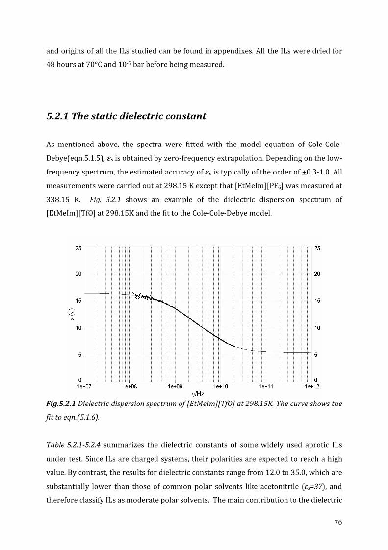
76
and origins of all the ILs studied can be found in appendixes. All the ILs were dried for
48 hours at 70°C and 10-5 bar before being measured.
5.2.1 The static dielectric constant
As mentioned above, the spectra were fitted with the model equation of Cole-Cole-
Debye(eqn.5.1.5), εs is obtained by zero-frequency extrapolation. Depending on the low-
frequency spectrum, the estimated accuracy of εs is typically of the order of +0.3-1.0. All
measurements were carried out at 298.15 K except that [EtMeIm][PF6] was measured at
338.15 K. Fig. 5.2.1 shows an example of the dielectric dispersion spectrum of
[EtMeIm][TfO] at 298.15K and the fit to the Cole-Cole-Debye model.
Fig.5.2.1 Dielectric dispersion spectrum of [EtMeIm][TfO] at 298.15K. The curve shows the
fit to eqn.(5.1.6).
Table 5.2.1-5.2.4 summarizes the dielectric constants of some widely used aprotic ILs
under test. Since ILs are charged systems, their polarities are expected to reach a high
value. By contrast, the results for dielectric constants range from 12.0 to 35.0, which are
substantially lower than those of common polar solvents like acetonitrile (εs=37), and
therefore classify ILs as moderate polar solvents. The main contribution to the dielectric
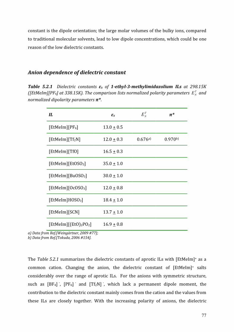
77
constant is the dipole orientation; the large molar volumes of the bulky ions, compared
to traditional molecular solvents, lead to low dipole concentrations, which could be one
reason of the low dielectric constants.
Anion dependence of dielectric constant
Table 5.2.1 Dielectric constants εs of 1-ethyl-3-methylimidazolium ILs at 298.15K ([EtMeIm][PF6] at 338.15K). The comparison lists normalized polarity parameters T
NE and normalized dipolarity parameters π*.
IL εs TNE π*
[EtMeIm][PF6] 13.0 + 0.5
[EtMeIm][Tf2N] 12.0 + 0.3 0.676a) 0.970b)
[EtMeIm][TfO] 16.5 + 0.3
[EtMeIm][EtOSO3] 35.0 + 1.0
[EtMeIm][BuOSO3] 30.0 + 1.0
[EtMeIm][OcOSO3] 12.0 + 0.8
[EtMeIm]HOSO3] 18.4 + 1.0
[EtMeIm][SCN] 13.7 + 1.0
[EtMeIm][(EtO)2PO2] 16.9 + 0.8
a) Data from Ref.[Weingärtner, 2009 #77]; b) Data from Ref.[Tokuda, 2006 #154]. The Table 5.2.1 summarizes the dielectric constants of aprotic ILs with [EtMeIm]+ as a
common cation. Changing the anion, the dielectric constant of [EtMeIm]+ salts
considerably over the range of aprotic ILs. For the anions with symmetric structure,
such as [BF4] -, [PF6] - and [Tf2N] -, which lack a permanent dipole moment, the
contribution to the dielectric constant mainly comes from the cation and the values from
these ILs are closely together. With the increasing polarity of anions, the dielectric
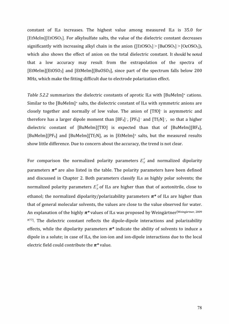
78
constant of ILs increases. The highest value among measured ILs is 35.0 for
[EtMeIm][EtOSO3]. For alkylsulfate salts, the value of the dielectric constant decreases
significantly with increasing alkyl chain in the anion ([EtOSO3] > [BuOSO3] > [OcOSO3]),
which also shows the effect of anion on the total dielectric constant. It should be noted
that a low accuracy may result from the extrapolation of the spectra of
[EtMeIm][EtOSO3] and [EtMeIm][BuOSO3], since part of the spectrum falls below 200
MHz, which make the fitting difficult due to electrode polarization effect.
Table 5.2.2 summarizes the dielectric constants of aprotic ILs with [BuMeIm]+ cations.
Similar to the [BuMeIm]+ salts, the dielectric constant of ILs with symmetric anions are
closely together and normally of low value. The anion of [TfO]- is asymmetric and
therefore has a larger dipole moment than [BF4] -, [PF6] - and [Tf2N] -, so that a higher
dielectric constant of [BuMeIm][TfO] is expected than that of [BuMeIm][BF4],
[BuMeIm][PF6] and [BuMeIm][Tf2N], as in [EtMeIm]+ salts, but the measured results
show little difference. Due to concern about the accuracy, the trend is not clear.
For comparison the normalized polarity parameters TNE and normalized dipolarity
parameters π* are also listed in the table. The polarity parameters have been defined
and discussed in Chapter 2. Both parameters classify ILs as highly polar solvents; the
normalized polarity parameters TNE of ILs are higher than that of acetonitrile, close to
ethanol; the normalized dipolarity/polarizability parameters π* of ILs are higher than
that of general molecular solvents, the values are close to the value observed for water.
An explanation of the highly π* values of ILs was proposed by Weingärtner[Weingärtner, 2009
#77]. The dielectric constant reflects the dipole-dipole interactions and polarizability
effects, while the dipolarity parameters π* indicate the ability of solvents to induce a
dipole in a solute; in case of ILs, the ion-ion and ion-dipole interactions due to the local
electric field could contribute the π* value.
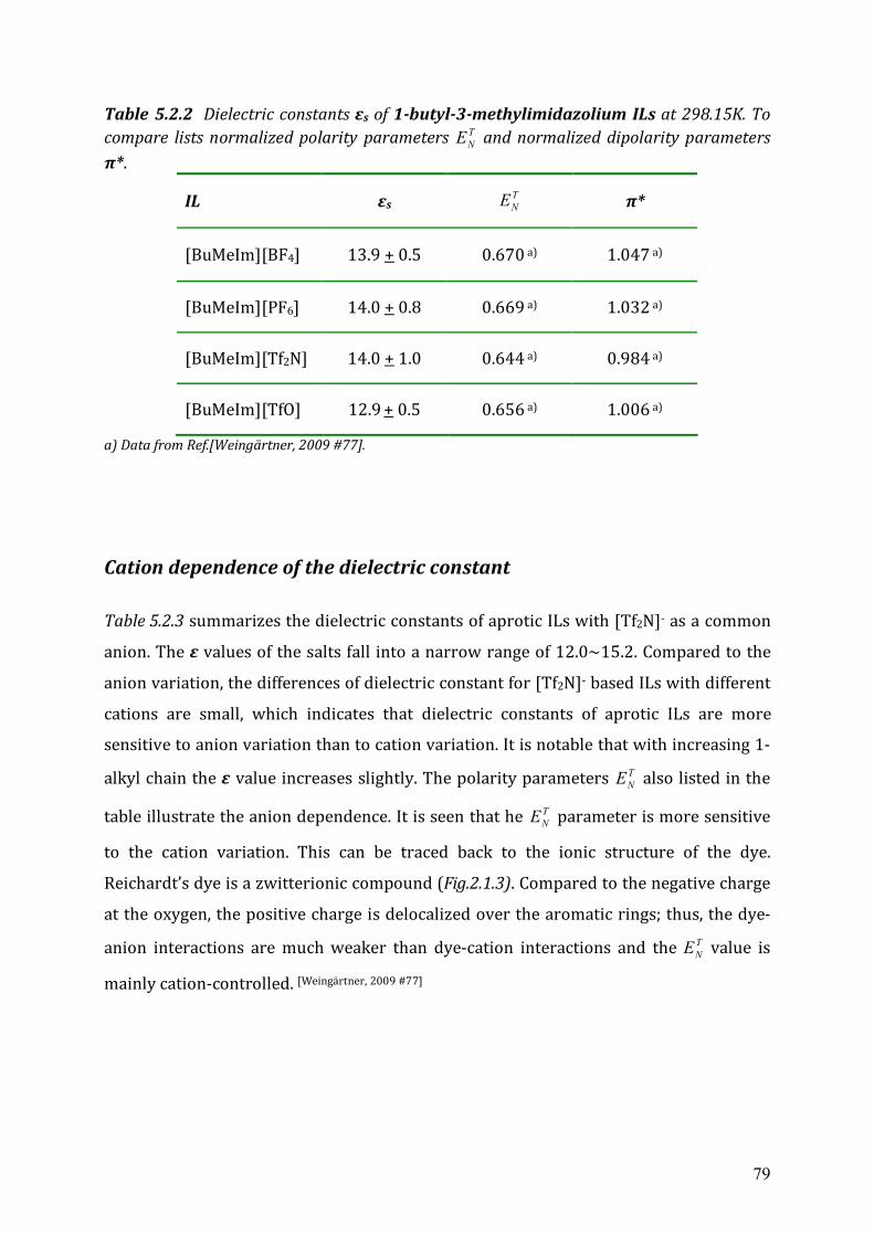
79
Table 5.2.2 Dielectric constants εs of 1-butyl-3-methylimidazolium ILs at 298.15K. To compare lists normalized polarity parameters T
NE and normalized dipolarity parameters π*.
IL εs TNE π*
[BuMeIm][BF4] 13.9 + 0.5 0.670 a) 1.047 a)
[BuMeIm][PF6] 14.0 + 0.8 0.669 a) 1.032 a)
[BuMeIm][Tf2N] 14.0 + 1.0 0.644 a) 0.984 a)
[BuMeIm][TfO] 12.9 + 0.5 0.656 a) 1.006 a)
a) Data from Ref.[Weingärtner, 2009 #77]. Cation dependence of the dielectric constant
Table 5.2.3 summarizes the dielectric constants of aprotic ILs with [Tf2N]- as a common
anion. The ε values of the salts fall into a narrow range of 12.0~15.2. Compared to the
anion variation, the differences of dielectric constant for [Tf2N]- based ILs with different
cations are small, which indicates that dielectric constants of aprotic ILs are more
sensitive to anion variation than to cation variation. It is notable that with increasing 1-
alkyl chain the ε value increases slightly. The polarity parameters TNE also listed in the
table illustrate the anion dependence. It is seen that he TNE parameter is more sensitive
to the cation variation. This can be traced back to the ionic structure of the dye.
Reichardt’s dye is a zwitterionic compound (Fig.2.1.3). Compared to the negative charge
at the oxygen, the positive charge is delocalized over the aromatic rings; thus, the dye-
anion interactions are much weaker than dye-cation interactions and the TNE value is
mainly cation-controlled. [Weingärtner, 2009 #77]
80
Table 5.2.3 Dielectric constants εs of bis(trifluoromethylsulfonyl)amide ILs at 298.15K. For comparison the table lists normalized polarity parameters T
NE and normalized dipolarity parameters π*.
IL εs TNE π*
[EtMeIm] [Tf2N] 12.0 + 0.3 0.676 a) 0.970b)
[EtMeMeIm][Tf2N] 12.8 + 0.3
[PrMeIm][Tf2N] 13.3 + 0.3 0.654 a)
[BuMeIm] [Tf2N] 14.0 + 1.0 0.596 a) 0.984 a)
[BuMeMeIm][Tf2N] 14.0 + 0.5 0.546 a)
[PeMeIm] [Tf2N] 15.0+ 0.5
[BuPy] [Tf2N] 15.2 + 0.3 0.648 a 1.01b
[PeMePyr] [Tf2N] 12.5 + 0.5
[PeEt3N] [Tf2N] 12.5 + 0.5
a) Data from Ref.[Weingärtner, 2009 #77]; b) Data from Ref.[Tokuda, 2006 #154]. ILs based on methyl-substituted imidazolium cations 1-alkyl-3-methylimidazolium is an aromatic cation with a delocalized 3-center-4-
electron configuration across the N1-C2-N3 moiety, a double bond between C4 and C5
and a weak delocalization in the central region[Weingärtner, 2008 #49]. C2 is positively charged
owing to the electron deficit in the C=N bond, whereas C4 and C5 are practically
neutral[Weingärtner, 2008 #49]. It has been proved experimentally that all three protons at C2,
C4 and C5 are acidic, and the C2 proton is more potential to be a hydrogen bond donor
towards anions[Elaiwi, 1995 #104].
Table 5.2.4 summarizes the dielectric constants of ILs based on methyl-substituted
imidazolium cations. Replacement of the proton at C2 position yields [EtMeMeIm]+ and
[BuMeMeIm]+ cations; replacement of the protons at C2, C4 and C5 positions yields
[BuMe4Im]+ cation. The former was obtained from IoLiTec (Denzlingen, Germany), the
latter were synthesized.
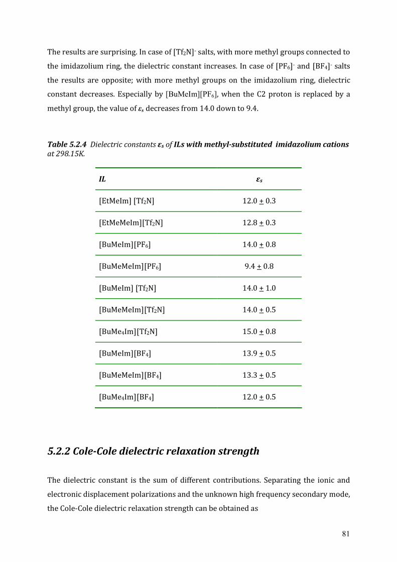
81
The results are surprising. In case of [Tf2N]- salts, with more methyl groups connected to
the imidazolium ring, the dielectric constant increases. In case of [PF6]- and [BF4]- salts
the results are opposite; with more methyl groups on the imidazolium ring, dielectric
constant decreases. Especially by [BuMeIm][PF6], when the C2 proton is replaced by a
methyl group, the value of εs decreases from 14.0 down to 9.4.
Table 5.2.4 Dielectric constants εs of ILs with methyl-substituted imidazolium cations at 298.15K.
IL εs
[EtMeIm] [Tf2N] 12.0 + 0.3
[EtMeMeIm][Tf2N] 12.8 + 0.3
[BuMeIm][PF6] 14.0 + 0.8
[BuMeMeIm][PF6] 9.4 + 0.8
[BuMeIm] [Tf2N] 14.0 + 1.0
[BuMeMeIm][Tf2N] 14.0 + 0.5
[BuMe4Im][Tf2N] 15.0 + 0.8
[BuMeIm][BF4] 13.9 + 0.5
[BuMeMeIm][BF4] 13.3 + 0.5
[BuMe4Im][BF4] 12.0 + 0.5
5.2.2 Cole-Cole dielectric relaxation strength
The dielectric constant is the sum of different contributions. Separating the ionic and
electronic displacement polarizations and the unknown high frequency secondary mode,
the Cole-Cole dielectric relaxation strength can be obtained as
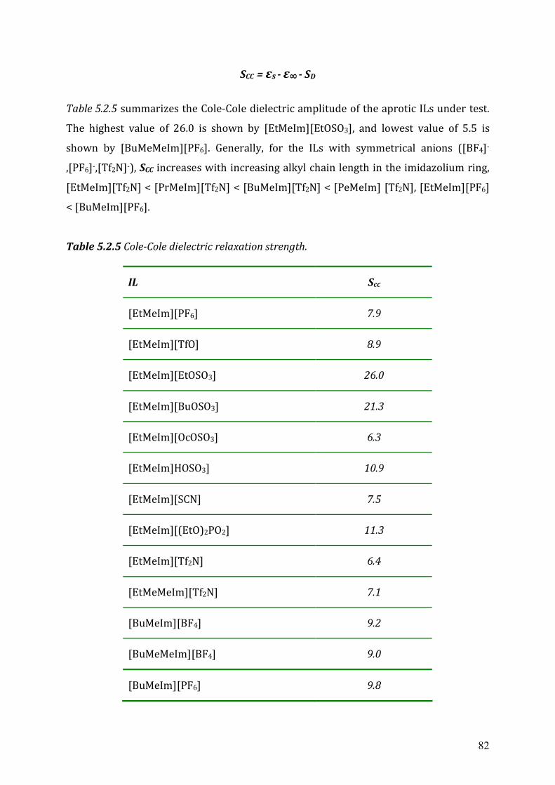
82
SCC = εs - ε∞ - SD
Table 5.2.5 summarizes the Cole-Cole dielectric amplitude of the aprotic ILs under test.
The highest value of 26.0 is shown by [EtMeIm][EtOSO3], and lowest value of 5.5 is
shown by [BuMeMeIm][PF6]. Generally, for the ILs with symmetrical anions ([BF4]-
,[PF6]-,[Tf2N]-), SCC increases with increasing alkyl chain length in the imidazolium ring,
[EtMeIm][Tf2N] < [PrMeIm][Tf2N] < [BuMeIm][Tf2N] < [PeMeIm] [Tf2N], [EtMeIm][PF6]
< [BuMeIm][PF6].
Table 5.2.5 Cole-Cole dielectric relaxation strength.
IL Scc
[EtMeIm][PF6] 7.9
[EtMeIm][TfO] 8.9
[EtMeIm][EtOSO3] 26.0
[EtMeIm][BuOSO3] 21.3
[EtMeIm][OcOSO3] 6.3
[EtMeIm]HOSO3] 10.9
[EtMeIm][SCN] 7.5
[EtMeIm][(EtO)2PO2] 11.3
[EtMeIm][Tf2N] 6.4
[EtMeMeIm][Tf2N] 7.1
[BuMeIm][BF4] 9.2
[BuMeMeIm][BF4] 9.0
[BuMe4Im][BF4] 6.9 [BuMeIm][PF6] 9.8
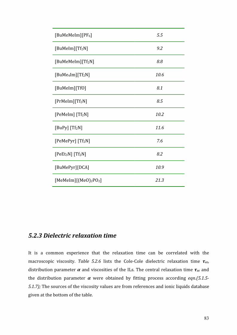
83
5.2.3 Dielectric relaxation time
It is a common experience that the relaxation time can be correlated with the
macroscopic viscosity. Table 5.2.6 lists the Cole-Cole dielectric relaxation time τcc,
distribution parameter α and viscosities of the ILs. The central relaxation time τcc and
the distribution parameter α were obtained by fitting process according eqn.(5.1.5-
5.1.7); The sources of the viscosity values are from references and ionic liquids database
given at the bottom of the table.
[BuMeMeIm][PF6] 5.5
[BuMeIm][Tf2N] 9.2
[BuMeMeIm][Tf2N] 8.8
[BuMe4Im][Tf2N] 10.6
[BuMeIm][TfO] 8.1
[PrMeIm][Tf2N] 8.5
[PeMeIm] [Tf2N] 10.2
[BuPy] [Tf2N] 11.6
[PeMePyr] [Tf2N] 7.6
[PeEt3N] [Tf2N] 8.2
[BuMePyr][DCA] 10.9
[MeMeIm][(MeO)2PO2] 21.3
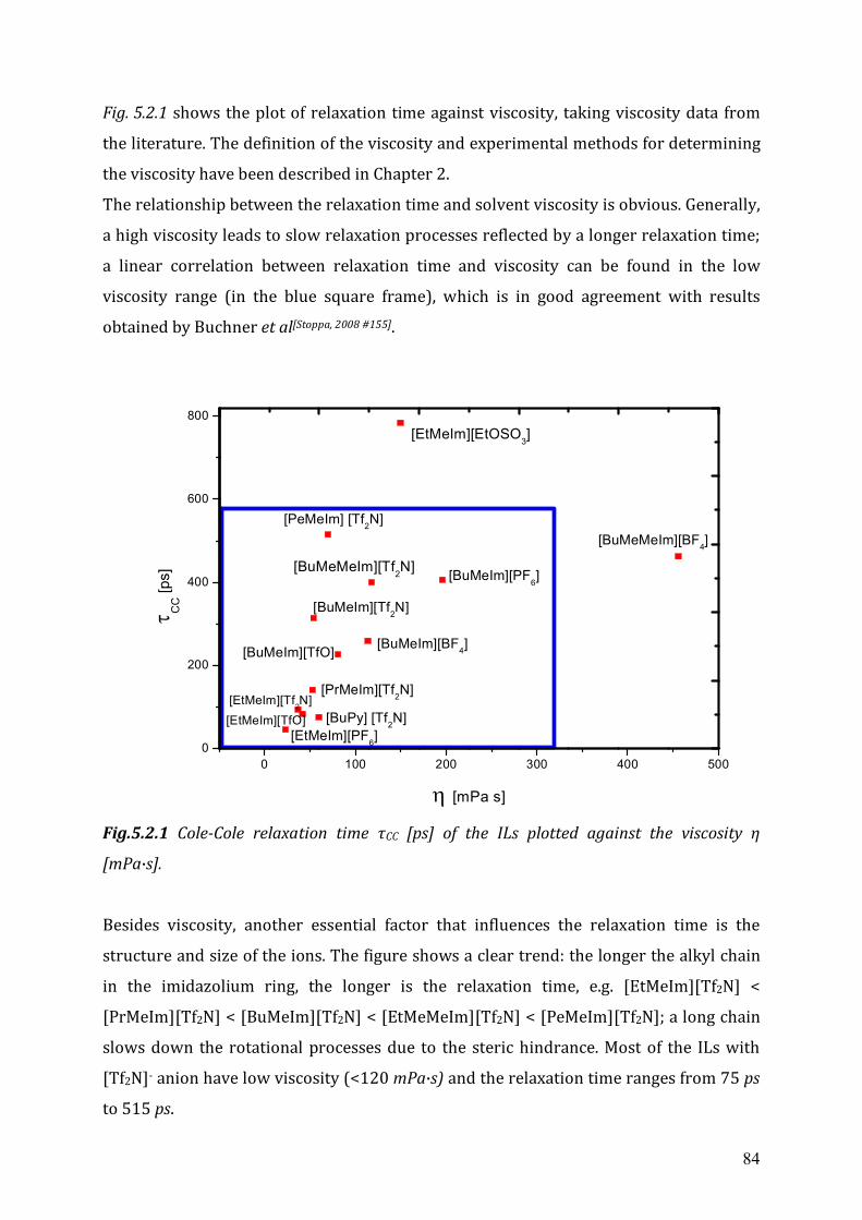
84
Fig. 5.2.1 shows the plot of relaxation time against viscosity, taking viscosity data from
the literature. The definition of the viscosity and experimental methods for determining
the viscosity have been described in Chapter 2.
The relationship between the relaxation time and solvent viscosity is obvious. Generally,
a high viscosity leads to slow relaxation processes reflected by a longer relaxation time;
a linear correlation between relaxation time and viscosity can be found in the low
viscosity range (in the blue square frame), which is in good agreement with results
obtained by Buchner et al[Stoppa, 2008 #155].
0 100 200 300 400 5000
200
400
600
800
CC [p
s]
[mPa s]
[BuMeIm][PF6]
[EtMeIm][EtOSO3]
[PeMeIm] [Tf2N]
[BuMeMeIm][Tf2N]
[BuMeMeIm][BF4]
[BuMeIm][Tf2N]
[BuMeIm][BF4][BuMeIm][TfO]
[PrMeIm][Tf2N]
[BuPy] [Tf2N][EtMeIm][PF
6]
[EtMeIm][Tf2N][EtMeIm][TfO]
Fig.5.2.1 Cole-Cole relaxation time τCC [ps] of the ILs plotted against the viscosity η
[mPa∙s].
Besides viscosity, another essential factor that influences the relaxation time is the
structure and size of the ions. The figure shows a clear trend: the longer the alkyl chain
in the imidazolium ring, the longer is the relaxation time, e.g. [EtMeIm][Tf2N] <
[PrMeIm][Tf2N] < [BuMeIm][Tf2N] < [EtMeMeIm][Tf2N] < [PeMeIm][Tf2N]; a long chain
slows down the rotational processes due to the steric hindrance. Most of the ILs with
[Tf2N]- anion have low viscosity (<120 mPa∙s) and the relaxation time ranges from 75 ps
to 515 ps.
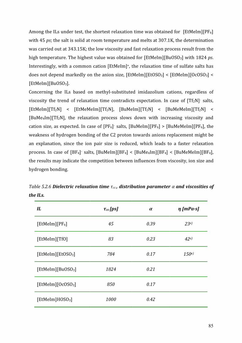
85
Among the ILs under test, the shortest relaxation time was obtained for [EtMeIm][PF6]
with 45 ps; the salt is solid at room temperature and melts at 307.1K, the determination
was carried out at 343.15K; the low viscosity and fast relaxation process result from the
high temperature. The highest value was obtained for [EtMeIm][BuOSO3] with 1824 ps.
Interestingly, with a common cation [EtMeIm]+, the relaxation time of sulfate salts has
does not depend markedly on the anion size, [EtMeIm][EtOSO3] < [EtMeIm][OcOSO3] <
[EtMeIm][BuOSO3].
Concerning the ILs based on methyl-substituted imidazolium cations, regardless of
viscosity the trend of relaxation time contradicts expectation. In case of [Tf2N]- salts,
[EtMeIm][Tf2N] < [EtMeMeIm][Tf2N], [BuMeIm][Tf2N] < [BuMeMeIm][Tf2N] <
[BuMe4Im][Tf2N], the relaxation process slows down with increasing viscosity and
cation size, as expected. In case of [PF6]- salts, [BuMeIm][PF6] > [BuMeMeIm][PF6], the
weakness of hydrogen bonding of the C2 proton towards anions replacement might be
an explanation, since the ion pair size is reduced, which leads to a faster relaxation
process. In case of [BF4]- salts, [BuMeIm][BF4] < [BuMe4Im][BF4] < [BuMeMeIm][BF4],
the results may indicate the competition between influences from viscosity, ion size and
hydrogen bonding.
Table 5.2.6 Dielectric relaxation time τcc , distribution parameter α and viscosities of
the ILs.
IL τcc [ps] α η [mPa∙s]
[EtMeIm][PF6] 45 0.39 23e)
[EtMeIm][TfO] 83 0.23 42e)
[EtMeIm][EtOSO3] 784 0.17 150e)
[EtMeIm][BuOSO3] 1824 0.21
[EtMeIm][OcOSO3] 850 0.17
[EtMeIm]HOSO3] 1000 0.42
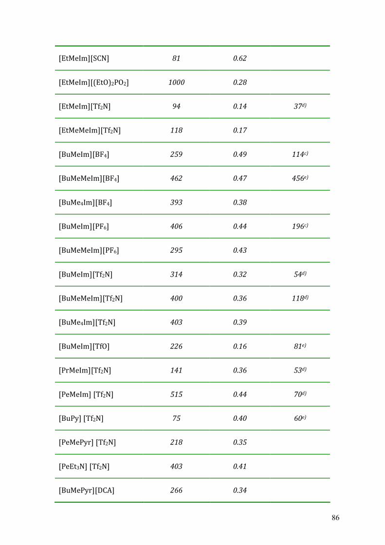
86
[EtMeIm][SCN] 81 0.62
[EtMeIm][(EtO)2PO2] 1000 0.28
[EtMeIm][Tf2N] 94 0.14 37d)
[EtMeMeIm][Tf2N] 118 0.17
[BuMeIm][BF4] 259 0.49 114c)
[BuMeMeIm][BF4] 462 0.47 456e)
[BuMe4Im][BF4] 393 0.38
[BuMeIm][PF6] 406 0.44 196c)
[BuMeMeIm][PF6] 295 0.43
[BuMeIm][Tf2N] 314 0.32 54d)
[BuMeMeIm][Tf2N] 400 0.36 118d)
[BuMe4Im][Tf2N] 403 0.39
[BuMeIm][TfO] 226 0.16 81e)
[PrMeIm][Tf2N] 141 0.36 53d)
[PeMeIm] [Tf2N] 515 0.44 70d)
[BuPy] [Tf2N] 75 0.40 60e)
[PeMePyr] [Tf2N] 218 0.35
[PeEt3N] [Tf2N] 403 0.41
[BuMePyr][DCA] 266 0.34
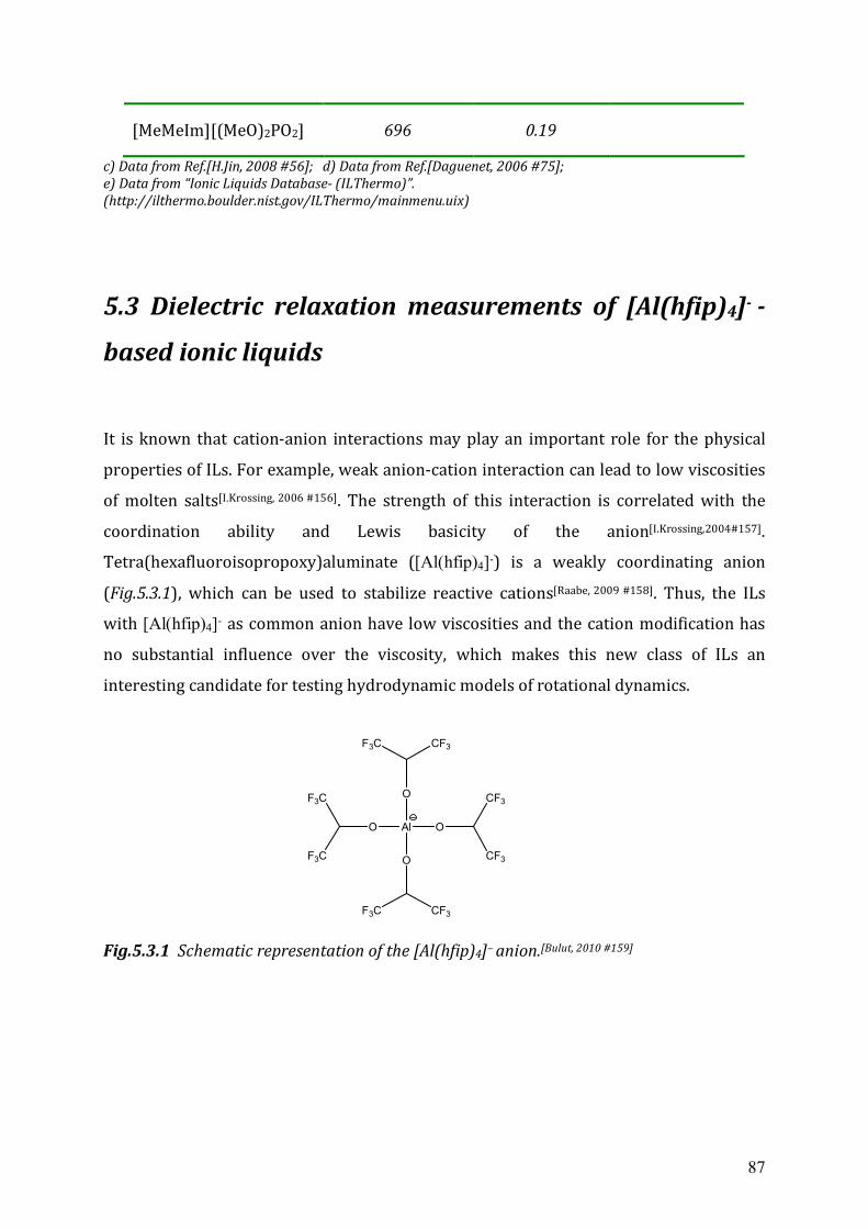
87
c) Data from Ref.[H.Jin, 2008 #56]; d) Data from Ref.[Daguenet, 2006 #75]; e) Data from “Ionic Liquids Database- (ILThermo)”. (http://ilthermo.boulder.nist.gov/ILThermo/mainmenu.uix)
5.3 Dielectric relaxation measurements of [Al(hfip)4]- -
based ionic liquids It is known that cation-anion interactions may play an important role for the physical
properties of ILs. For example, weak anion-cation interaction can lead to low viscosities
of molten salts[I.Krossing, 2006 #156]. The strength of this interaction is correlated with the
coordination ability and Lewis basicity of the anion[I.Krossing,2004#157].
Tetra(hexafluoroisopropoxy)aluminate ([Al(hfip)4]-) is a weakly coordinating anion
(Fig.5.3.1), which can be used to stabilize reactive cations[Raabe, 2009 #158]. Thus, the ILs
with [Al(hfip)4]- as common anion have low viscosities and the cation modification has
no substantial influence over the viscosity, which makes this new class of ILs an
interesting candidate for testing hydrodynamic models of rotational dynamics.
Al
O
O
O
O
CF3F3C
CF3F3C
F3C
F3C
CF3
CF3
Fig.5.3.1 Schematic representation of the [Al(hfip)4]– anion.[Bulut, 2010 #159]
[MeMeIm][(MeO)2PO2] 696 0.19
88
5.3.1 Synthesis
In this work, a series of ILs with [Al(hfip)4] – as common anion were studied. These ILs
were synthesized by the group of I. Krossing at the Albert-Ludwig-University in
Freiburg. The anion metathesis was carried out in absolute CH2Cl2, using Li[Al(hfip)4]
and methylimidazolium halides (Cl– or Br–) as starting materials. The reaction was
conducted for 24 hours at room temperature, followed by filtration of the reaction
mixture and removal of CH2Cl2. Products were rinsed with n-hexane and dried for 24
hours under vacuum. Since [Al(hfip)4]– is water-sensitive, all the steps were conducted
under inert conditions. Details of the synthesis can be found in Ref. [Bulut, 2010 #159] .
5.3.2 Dielectric measurements and data evaluation
All the ILs were tested at temperature of (343.1 0.2) K, which is well above their
melting temperatures. The working frequency ranges from 50MHz up to 20GHz. Fig.5.3.2
shows the experimental recorded real- and total imaginary part of complex dielectric
function of [BuMeMorph][Al(hfip)4].
The spectra were fitted to the Cole-Cole-Debye function (5.1.5). Dielectric relaxation
probes the collective response of all dipoles, and so does the relaxation time τCC
obtained through fitting. By contrast, hydrodynamic theory relates the single-particle
reorientation time Lrot to the viscous friction exerted by the surrounding medium[Dote,
1981 #160]. Thus, to apply the hydrodynamic relations, τCC needs first to be converted
to Lrot . The conversion between τCC and L
rot is given by [Glarum, 1960 #161]
CCLrot
1
32
(5.3.1)
where it is estimated that 22 n , as predicted by the Maxwell-relation.
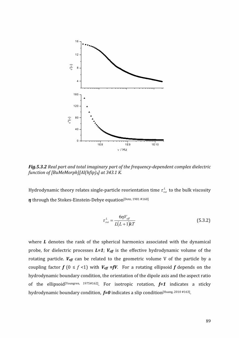
89
1E8 1E9 1E100
40
80
120
160
4
8
12
16
''(
)
/ Hz
'()
Fig.5.3.2 Real part and total imaginary part of the frequency-dependent complex dielectric function of [BuMeMorph][Al(hfip)4] at 343.1 K. Hydrodynamic theory relates single-particle reorientation time L
rot to the bulk viscosity
η through the Stokes-Einstein-Debye equation[Dote, 1981 #160]
kTLLVeffL
rot 16
(5.3.2)
where L denotes the rank of the spherical harmonics associated with the dynamical
probe, for dielectric processes L=1; Veff is the effective hydrodynamic volume of the
rotating particle. Veff can be related to the geometric volume V of the particle by a
coupling factor f (0 ≤ f <1) with Veff =fV. For a rotating ellipsoid f depends on the
hydrodynamic boundary condition, the orientation of the dipole axis and the aspect ratio
of the ellipsoid[Youngren, 1975#162]. For isotropic rotation, f=1 indicates a sticky
hydrodynamic boundary condition, f=0 indicates a slip condition[Huang, 2010 #163].
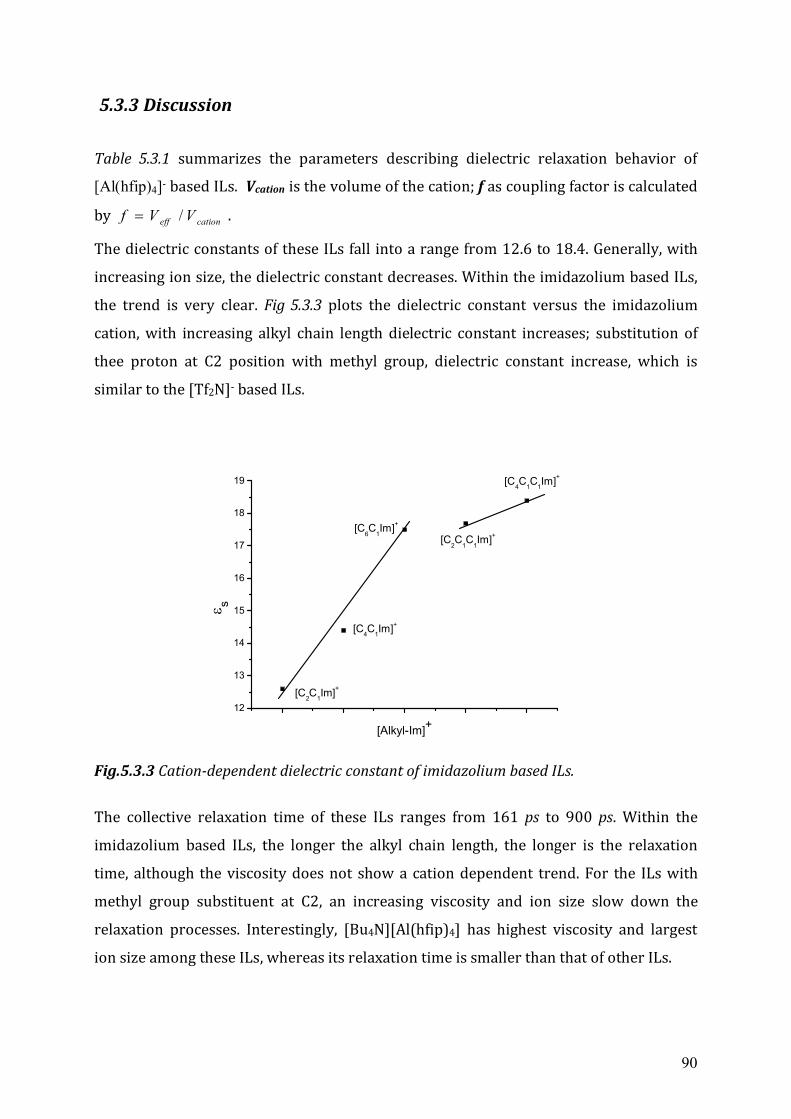
90
5.3.3 Discussion
Table 5.3.1 summarizes the parameters describing dielectric relaxation behavior of
[Al(hfip)4]- based ILs. Vcation is the volume of the cation; f as coupling factor is calculated
by cationeff VVf / .
The dielectric constants of these ILs fall into a range from 12.6 to 18.4. Generally, with
increasing ion size, the dielectric constant decreases. Within the imidazolium based ILs,
the trend is very clear. Fig 5.3.3 plots the dielectric constant versus the imidazolium
cation, with increasing alkyl chain length dielectric constant increases; substitution of
thee proton at C2 position with methyl group, dielectric constant increase, which is
similar to the [Tf2N]- based ILs.
12
13
14
15
16
17
18
19
s
[Alkyl-Im]+
[C2C1Im]+
[C4C1Im]+
[C6C
1Im]+
[C2C
1C
1Im]+
[C4C1C1Im]+
Fig.5.3.3 Cation-dependent dielectric constant of imidazolium based ILs.
The collective relaxation time of these ILs ranges from 161 ps to 900 ps. Within the
imidazolium based ILs, the longer the alkyl chain length, the longer is the relaxation
time, although the viscosity does not show a cation dependent trend. For the ILs with
methyl group substituent at C2, an increasing viscosity and ion size slow down the
relaxation processes. Interestingly, [Bu4N][Al(hfip)4] has highest viscosity and largest
ion size among these ILs, whereas its relaxation time is smaller than that of other ILs.
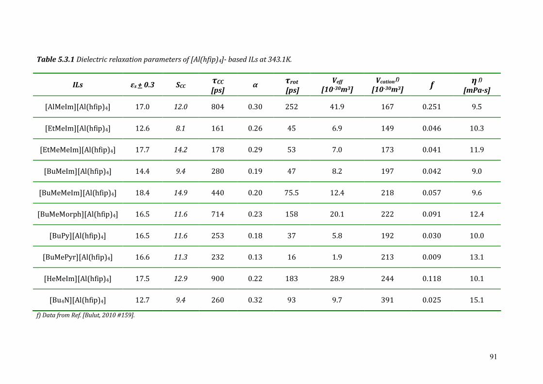
91
Table 5.3.1 Dielectric relaxation parameters of [Al(hfip)4]- based ILs at 343.1K.
ILs εs + 0.3 SCC τCC [ps]
α τrot [ps]
Veff [10-30m3]
Vcation f) [10-30m3] f η f)
[mPa∙s]
[AlMeIm][Al(hfip)4] 17.0 12.0 804 0.30 252 41.9 167 0.251 9.5
[EtMeIm][Al(hfip)4] 12.6 8.1 161 0.26 45 6.9 149 0.046 10.3
[EtMeMeIm][Al(hfip)4] 17.7 14.2 178 0.29 53 7.0 173 0.041 11.9
[BuMeIm][Al(hfip)4] 14.4 9.4 280 0.19 47 8.2 197 0.042 9.0
[BuMeMeIm][Al(hfip)4] 18.4 14.9 440 0.20 75.5 12.4 218 0.057 9.6
[BuMeMorph][Al(hfip)4] 16.5 11.6 714 0.23 158 20.1 222 0.091 12.4
[BuPy][Al(hfip)4] 16.5 11.6 253 0.18 37 5.8 192 0.030 10.0
[BuMePyr][Al(hfip)4] 16.6 11.3 232 0.13 16 1.9 213 0.009 13.1
[HeMeIm][Al(hfip)4] 17.5 12.9 900 0.22 183 28.9 244 0.118 10.1
[Bu4N][Al(hfip)4] 12.7 9.4 260 0.32 93 9.7 391 0.025 15.1
f) Data from Ref. [Bulut, 2010 #159].
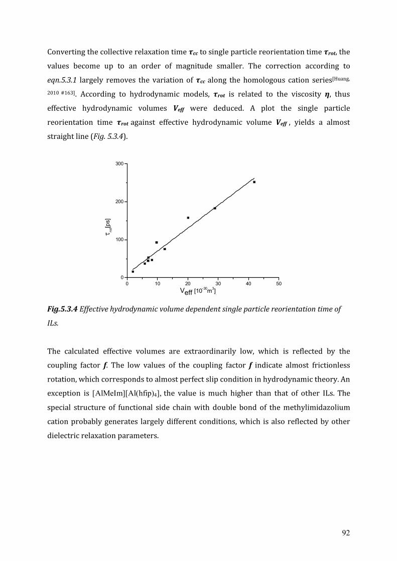
92
Converting the collective relaxation time τcc to single particle reorientation time τrot, the
values become up to an order of magnitude smaller. The correction according to
eqn.5.3.1 largely removes the variation of τcc along the homologous cation series[Huang,
2010 #163]. According to hydrodynamic models, τrot is related to the viscosity η, thus
effective hydrodynamic volumes Veff were deduced. A plot the single particle
reorientation time τrot against effective hydrodynamic volume Veff , yields a almost
straight line (Fig. 5.3.4).
0 10 20 30 40 500
100
200
300
rot[p
s]
Veff [10-30m3].
Fig.5.3.4 Effective hydrodynamic volume dependent single particle reorientation time of
ILs.
The calculated effective volumes are extraordinarily low, which is reflected by the
coupling factor f. The low values of the coupling factor f indicate almost frictionless
rotation, which corresponds to almost perfect slip condition in hydrodynamic theory. An
exception is [AlMeIm][Al(hfip)4], the value is much higher than that of other ILs. The
special structure of functional side chain with double bond of the methylimidazolium
cation probably generates largely different conditions, which is also reflected by other
dielectric relaxation parameters.
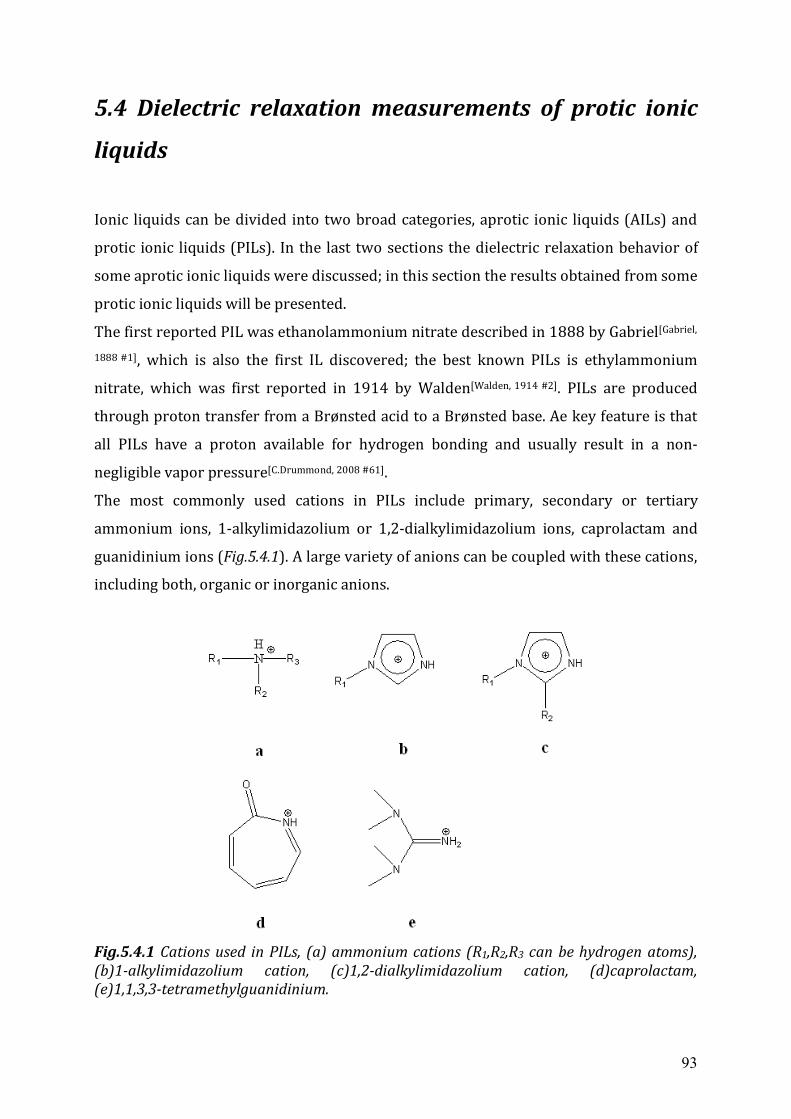
93
5.4 Dielectric relaxation measurements of protic ionic
liquids
Ionic liquids can be divided into two broad categories, aprotic ionic liquids (AILs) and
protic ionic liquids (PILs). In the last two sections the dielectric relaxation behavior of
some aprotic ionic liquids were discussed; in this section the results obtained from some
protic ionic liquids will be presented.
The first reported PIL was ethanolammonium nitrate described in 1888 by Gabriel[Gabriel,
1888 #1], which is also the first IL discovered; the best known PILs is ethylammonium
nitrate, which was first reported in 1914 by Walden[Walden, 1914 #2]. PILs are produced
through proton transfer from a Brønsted acid to a Brønsted base. Ae key feature is that
all PILs have a proton available for hydrogen bonding and usually result in a non-
negligible vapor pressure[C.Drummond, 2008 #61].
The most commonly used cations in PILs include primary, secondary or tertiary
ammonium ions, 1-alkylimidazolium or 1,2-dialkylimidazolium ions, caprolactam and
guanidinium ions (Fig.5.4.1). A large variety of anions can be coupled with these cations,
including both, organic or inorganic anions.
Fig.5.4.1 Cations used in PILs, (a) ammonium cations (R1,R2,R3 can be hydrogen atoms), (b)1-alkylimidazolium cation, (c)1,2-dialkylimidazolium cation, (d)caprolactam, (e)1,1,3,3-tetramethylguanidinium.
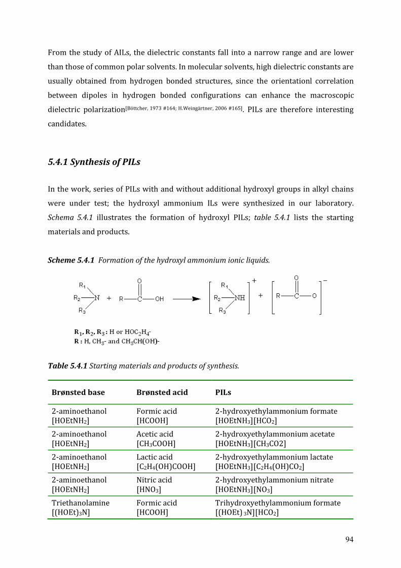
94
From the study of AILs, the dielectric constants fall into a narrow range and are lower
than those of common polar solvents. In molecular solvents, high dielectric constants are
usually obtained from hydrogen bonded structures, since the orientationl correlation
between dipoles in hydrogen bonded configurations can enhance the macroscopic
dielectric polarization[Böttcher, 1973 #164; H.Weingärtner, 2006 #165]. PILs are therefore interesting
candidates.
5.4.1 Synthesis of PILs
In the work, series of PILs with and without additional hydroxyl groups in alkyl chains
were under test; the hydroxyl ammonium ILs were synthesized in our laboratory.
Schema 5.4.1 illustrates the formation of hydroxyl PILs; table 5.4.1 lists the starting
materials and products.
Scheme 5.4.1 Formation of the hydroxyl ammonium ionic liquids.
Table 5.4.1 Starting materials and products of synthesis.
Brønsted base Brønsted acid PILs
2-aminoethanol [HOEtNH2]
Formic acid [HCOOH]
2-hydroxyethylammonium formate [HOEtNH3][HCO2]
2-aminoethanol [HOEtNH2]
Acetic acid [CH3COOH]
2-hydroxyethylammonium acetate [HOEtNH3][CH3CO2]
2-aminoethanol [HOEtNH2]
Lactic acid [C2H4(OH)COOH]
2-hydroxyethylammonium lactate [HOEtNH3][C2H4(OH)CO2]
2-aminoethanol [HOEtNH2]
Nitric acid [HNO3]
2-hydroxyethylammonium nitrate [HOEtNH3][NO3]
Triethanolamine [(HOEt)3N]
Formic acid [HCOOH]
Trihydroxyethylammonium formate [(HOEt) 3N][HCO2]
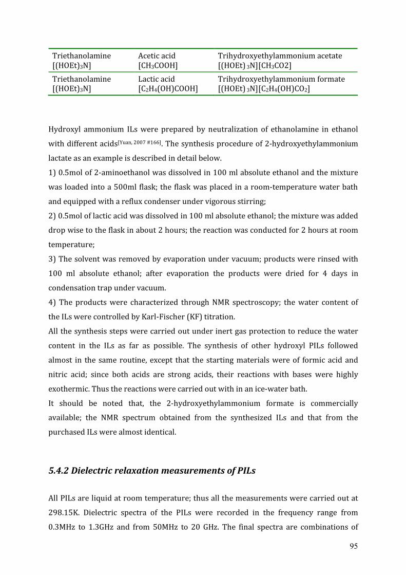
95
Triethanolamine [(HOEt)3N]
Acetic acid [CH3COOH]
Trihydroxyethylammonium acetate [(HOEt) 3N][CH3CO2]
Triethanolamine [(HOEt)3N]
Lactic acid [C2H4(OH)COOH]
Trihydroxyethylammonium formate [(HOEt) 3N][C2H4(OH)CO2]
Hydroxyl ammonium ILs were prepared by neutralization of ethanolamine in ethanol
with different acids[Yuan, 2007 #166]. The synthesis procedure of 2-hydroxyethylammonium
lactate as an example is described in detail below.
1) 0.5mol of 2-aminoethanol was dissolved in 100 ml absolute ethanol and the mixture
was loaded into a 500ml flask; the flask was placed in a room-temperature water bath
and equipped with a reflux condenser under vigorous stirring;
2) 0.5mol of lactic acid was dissolved in 100 ml absolute ethanol; the mixture was added
drop wise to the flask in about 2 hours; the reaction was conducted for 2 hours at room
temperature;
3) The solvent was removed by evaporation under vacuum; products were rinsed with
100 ml absolute ethanol; after evaporation the products were dried for 4 days in
condensation trap under vacuum.
4) The products were characterized through NMR spectroscopy; the water content of
the ILs were controlled by Karl-Fischer (KF) titration.
All the synthesis steps were carried out under inert gas protection to reduce the water
content in the ILs as far as possible. The synthesis of other hydroxyl PILs followed
almost in the same routine, except that the starting materials were of formic acid and
nitric acid; since both acids are strong acids, their reactions with bases were highly
exothermic. Thus the reactions were carried out with in an ice-water bath.
It should be noted that, the 2-hydroxyethylammonium formate is commercially
available; the NMR spectrum obtained from the synthesized ILs and that from the
purchased ILs were almost identical.
5.4.2 Dielectric relaxation measurements of PILs
All PILs are liquid at room temperature; thus all the measurements were carried out at
298.15K. Dielectric spectra of the PILs were recorded in the frequency range from
0.3MHz to 1.3GHz and from 50MHz to 20 GHz. The final spectra are combinations of
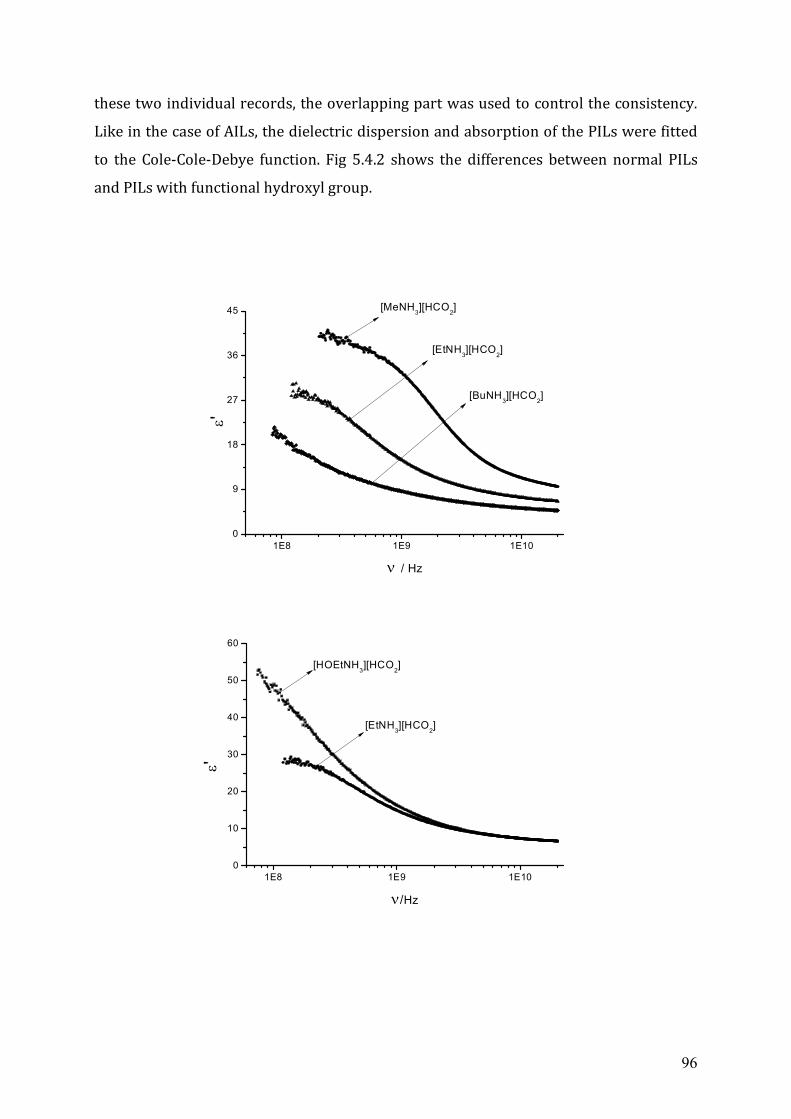
96
these two individual records, the overlapping part was used to control the consistency.
Like in the case of AILs, the dielectric dispersion and absorption of the PILs were fitted
to the Cole-Cole-Debye function. Fig 5.4.2 shows the differences between normal PILs
and PILs with functional hydroxyl group.
1E8 1E9 1E100
9
18
27
36
45
'
[BuNH3][HCO2]
[EtNH3][HCO2]
/ Hz
[MeNH3][HCO2]
1E8 1E9 1E100
10
20
30
40
50
60
[EtNH3][HCO2]
'
/Hz
[HOEtNH3][HCO2]
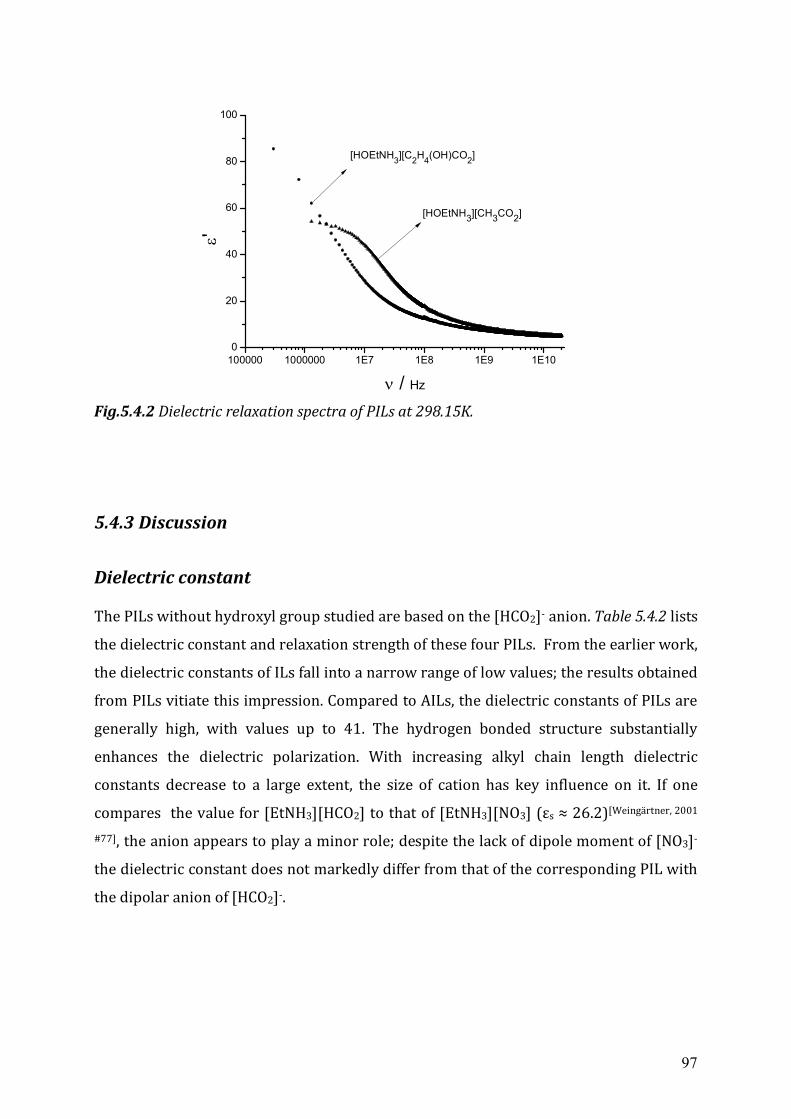
97
100000 1000000 1E7 1E8 1E9 1E100
20
40
60
80
100
'[HOEtNH3][CH3CO2]
/ Hz
[HOEtNH3][C2H4(OH)CO2]
Fig.5.4.2 Dielectric relaxation spectra of PILs at 298.15K.
5.4.3 Discussion
Dielectric constant The PILs without hydroxyl group studied are based on the [HCO2]- anion. Table 5.4.2 lists
the dielectric constant and relaxation strength of these four PILs. From the earlier work,
the dielectric constants of ILs fall into a narrow range of low values; the results obtained
from PILs vitiate this impression. Compared to AILs, the dielectric constants of PILs are
generally high, with values up to 41. The hydrogen bonded structure substantially
enhances the dielectric polarization. With increasing alkyl chain length dielectric
constants decrease to a large extent, the size of cation has key influence on it. If one
compares the value for [EtNH3][HCO2] to that of [EtNH3][NO3] (εs ≈ 26.2)[Weingärtner, 2001
#77], the anion appears to play a minor role; despite the lack of dipole moment of [NO3]-
the dielectric constant does not markedly differ from that of the corresponding PIL with
the dipolar anion of [HCO2]-.
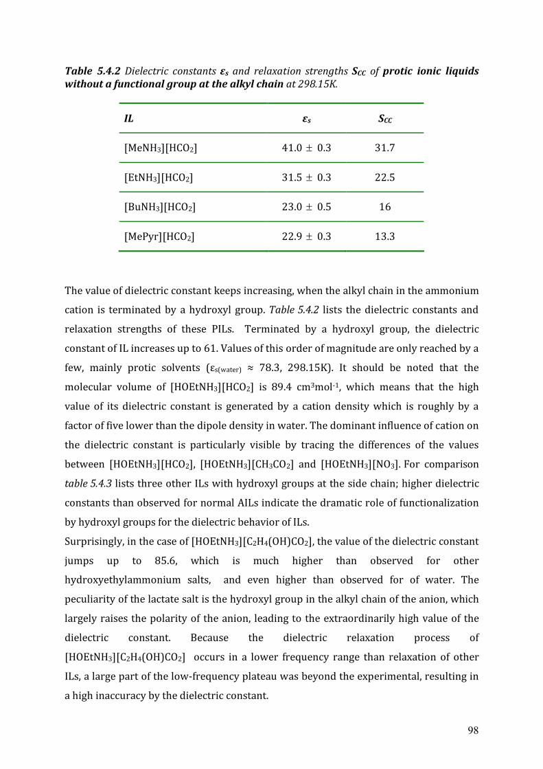
98
Table 5.4.2 Dielectric constants εs and relaxation strengths SCC of protic ionic liquids without a functional group at the alkyl chain at 298.15K.
IL εs SCC
[MeNH3][HCO2] 41.0 0.3 31.7
[EtNH3][HCO2] 31.5 0.3 22.5
[BuNH3][HCO2] 23.0 0.5 16
[MePyr][HCO2] 22.9 0.3 13.3
The value of dielectric constant keeps increasing, when the alkyl chain in the ammonium
cation is terminated by a hydroxyl group. Table 5.4.2 lists the dielectric constants and
relaxation strengths of these PILs. Terminated by a hydroxyl group, the dielectric
constant of IL increases up to 61. Values of this order of magnitude are only reached by a
few, mainly protic solvents (εs(water) ≈ 78.3, 298.15K). It should be noted that the
molecular volume of [HOEtNH3][HCO2] is 89.4 cm3mol-1, which means that the high
value of its dielectric constant is generated by a cation density which is roughly by a
factor of five lower than the dipole density in water. The dominant influence of cation on
the dielectric constant is particularly visible by tracing the differences of the values
between [HOEtNH3][HCO2], [HOEtNH3][CH3CO2] and [HOEtNH3][NO3]. For comparison
table 5.4.3 lists three other ILs with hydroxyl groups at the side chain; higher dielectric
constants than observed for normal AILs indicate the dramatic role of functionalization
by hydroxyl groups for the dielectric behavior of ILs.
Surprisingly, in the case of [HOEtNH3][C2H4(OH)CO2], the value of the dielectric constant
jumps up to 85.6, which is much higher than observed for other
hydroxyethylammonium salts, and even higher than observed for of water. The
peculiarity of the lactate salt is the hydroxyl group in the alkyl chain of the anion, which
largely raises the polarity of the anion, leading to the extraordinarily high value of the
dielectric constant. Because the dielectric relaxation process of
[HOEtNH3][C2H4(OH)CO2] occurs in a lower frequency range than relaxation of other
ILs, a large part of the low-frequency plateau was beyond the experimental, resulting in
a high inaccuracy by the dielectric constant.
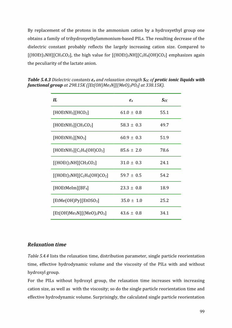
99
By replacement of the protons in the ammonium cation by a hydroxyethyl group one
obtains a family of trihydroxyethylammonium-based PILs. The resulting decrease of the
dielectric constant probably reflects the largely increasing cation size. Compared to
[(HOEt)3NH][CH3CO2], the high value for [(HOEt)3NH][C2H4(OH)CO2] emphasizes again
the peculiarity of the lactate anion.
Table 5.4.3 Dielectric constants εs and relaxation strength SCC of protic ionic liquids with functional group at 298.15K ([Et(OH)Me3N][(MeO)2PO2] at 338.15K).
IL εs SCC
[HOEtNH3][HCO2] 61.0 0.8 55.1
[HOEtNH3][CH3CO2] 58.3 0.3 49.7
[HOEtNH3][NO3] 60.9 0.3 51.9
[HOEtNH3][C2H4(OH)CO2] 85.6 2.0 78.6
[(HOEt)3NH][CH3CO2] 31.0 0.3 24.1
[(HOEt)3NH][C2H4(OH)CO2] 59.7 0.5 54.2
[HOEtMeIm][BF4] 23.3 0.8 18.9
[EtMe(OH)Py][EtOSO3] 35.0 1.0 25.2
[Et(OH)Me3N][(MeO)2PO2] 43.6 0.8 34.1
Relaxation time Table 5.4.4 lists the relaxation time, distribution parameter, single particle reorientation
time, effective hydrodynamic volume and the viscosity of the PILs with and without
hydroxyl group.
For the PILs without hydroxyl group, the relaxation time increases with increasing
cation size, as well as with the viscosity; so do the single particle reorientation time and
effective hydrodynamic volume. Surprisingly, the calculated single particle reorientation
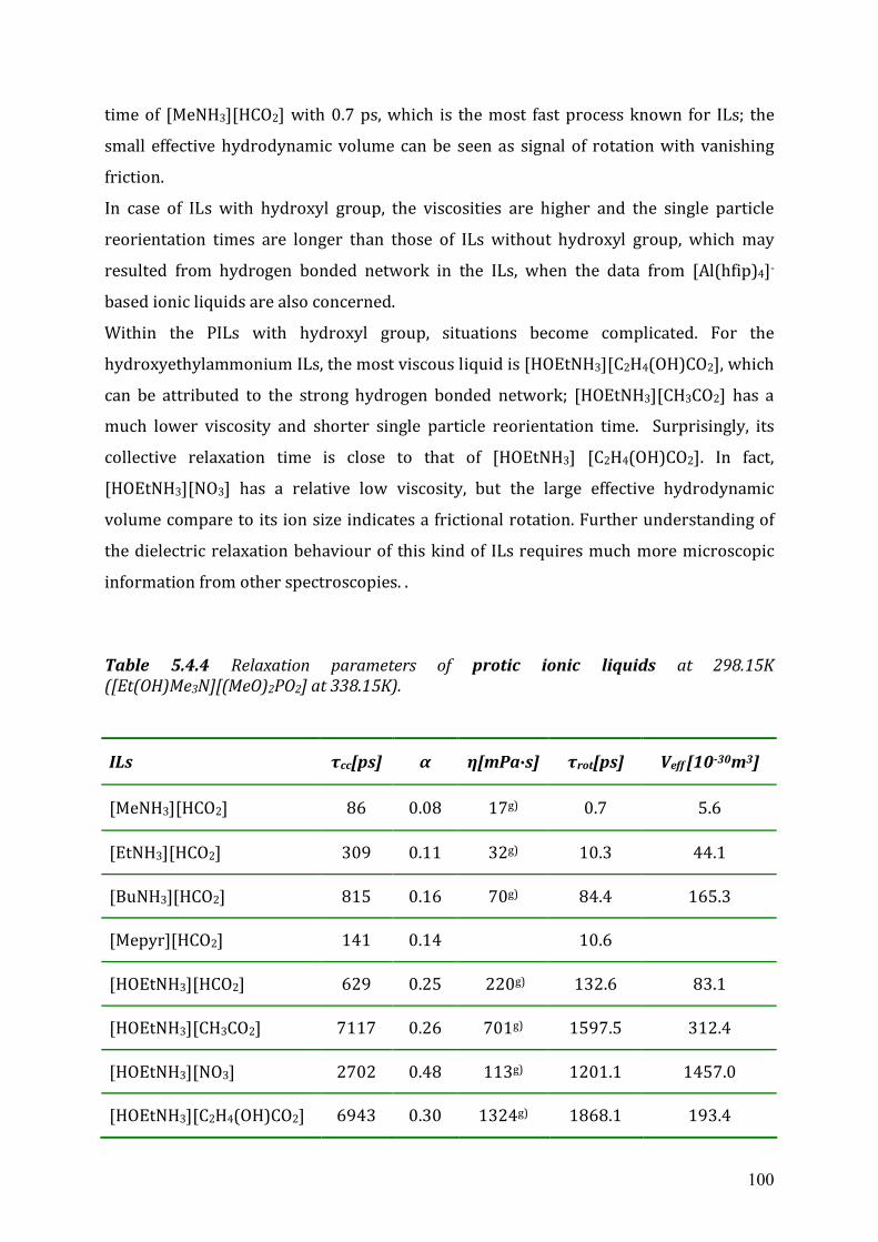
100
time of [MeNH3][HCO2] with 0.7 ps, which is the most fast process known for ILs; the
small effective hydrodynamic volume can be seen as signal of rotation with vanishing
friction.
In case of ILs with hydroxyl group, the viscosities are higher and the single particle
reorientation times are longer than those of ILs without hydroxyl group, which may
resulted from hydrogen bonded network in the ILs, when the data from [Al(hfip)4]-
based ionic liquids are also concerned.
Within the PILs with hydroxyl group, situations become complicated. For the
hydroxyethylammonium ILs, the most viscous liquid is [HOEtNH3][C2H4(OH)CO2], which
can be attributed to the strong hydrogen bonded network; [HOEtNH3][CH3CO2] has a
much lower viscosity and shorter single particle reorientation time. Surprisingly, its
collective relaxation time is close to that of [HOEtNH3] [C2H4(OH)CO2]. In fact,
[HOEtNH3][NO3] has a relative low viscosity, but the large effective hydrodynamic
volume compare to its ion size indicates a frictional rotation. Further understanding of
the dielectric relaxation behaviour of this kind of ILs requires much more microscopic
information from other spectroscopies. .
Table 5.4.4 Relaxation parameters of protic ionic liquids at 298.15K ([Et(OH)Me3N][(MeO)2PO2] at 338.15K).
ILs τcc[ps] α η[mPa∙s] τrot[ps] Veff [10-30m3]
[MeNH3][HCO2] 86 0.08 17g) 0.7 5.6
[EtNH3][HCO2] 309 0.11 32g) 10.3 44.1
[BuNH3][HCO2] 815 0.16 70g) 84.4 165.3
[Mepyr][HCO2] 141 0.14 10.6
[HOEtNH3][HCO2] 629 0.25 220g) 132.6 83.1
[HOEtNH3][CH3CO2] 7117 0.26 701g) 1597.5 312.4
[HOEtNH3][NO3] 2702 0.48 113g) 1201.1 1457.0
[HOEtNH3][C2H4(OH)CO2] 6943 0.30 1324g) 1868.1 193.4
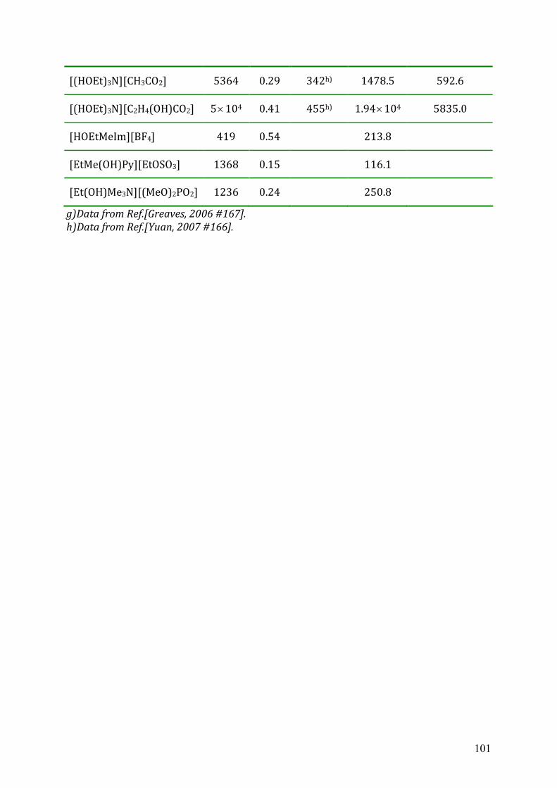
101
[(HOEt)3N][CH3CO2] 5364 0.29 342h) 1478.5 592.6
[(HOEt)3N][C2H4(OH)CO2] 5104 0.41 455h) 1.94104 5835.0
[HOEtMeIm][BF4] 419 0.54 213.8
[EtMe(OH)Py][EtOSO3] 1368 0.15 116.1
[Et(OH)Me3N][(MeO)2PO2] 1236 0.24 250.8
g)Data from Ref.[Greaves, 2006 #167]. h)Data from Ref.[Yuan, 2007 #166].
102
Chapter 6 Conclusions and Outlook Within the scope of this thesis, a series of homogenous ionic liquids were studied by
means of frequency dependent dielectric relaxation spectroscopy in microwave range
between 0.3MHz and 20 GHz.
The microwave dielectric spectrum is recorded in form of the complex dielectric
permittivity, which is separated into its real part ε’(ν) and imaginary part ε’’(ν).
Spectral analysis indicated a combination of two processes, represented by a model
based on a Cole-Cole relaxtion time distribution supplemented by a high-frequency
correction modelled by a Debye function. In this way, the static dielectric constant,
relaxation strength, relaxation time and distribution parameter are obtained.
Ionic liquids are divided into two families, non-protic ILs and protic ILs. The static
dielectric constants of protic ILs are commonly higher than those of non-protic ILs; the
hydrogen bonded structure substantially enhances the dielectric polarization. The
values of non-protic ILs are generally lower than εst = 30. In case of normal protic ILs
alued up to 41 were reached. Protic ILs with functional hydroxyl groups showed even
higher values, culminating in a value of 85.6 for [HOEtNH3][C2H4(OH)CO2]. Obviously,
the hydroxyl group in the alkyl chain of the anion highly raises the polarity of the anion,
thus increasing the dielectric constant.
For non-protic ILs, dielectric constants εst are more sensitive to anion variation than to
cation variation; with the increasing 1-alkyl chain on the imidazolium ring the value of
εst increases slightly; similar results are also obtained for [Al(hfip)4]- based ILs. ILs
based on methyl-substituted imidazolium cations do not show a clear tendency. Unlike
the non-protic ILs, the sensitivity of dielectric constants εst of protic ILs to anions and
cations are quite unsystematic.
The data of central relaxation time of ILs show a linear-like correlation to the viscosities
in the low viscosity range. Another essential factor that influences the relaxation time is
the structure and size of the ions; the longer the alkyl chain in the imidazolium rings, the
longer is the relaxation time.
103
In summarizing the experimental results dielectric relaxation spectroscopy is a powerful
tool for characterizing the dielectric behaviour of ILs, including information on the
solvent polarity provided by the dielectric constant. Polarity reflects a complex interplay
of all intermolecular interactions. Different experiments highlight different facets. The
dielectric constant of ILs mainly reflects the reorientational dipolar polarization of the
ions. Comparing the polarity parameters from different experimental methods can help
to learn more about the many molecular facets. Another interesting information involved in dielectric spectra concerns solvation
dynamics. This thesis focuses mainly on neat ILs. For a better understanding of solvation
dynamics, it could be helpful to expand the dielectric experiments to aqueous solutions
of ILs and to mixtures of ILs with organic solvents. In the thesis, most the measurements were carried out at room temperature. The
temperature dependent dielectric behaviour of ILs might reveal more information on
the ILs properties. Notably, a more general picture of the static and dynamic solvation propertied of ILs
requires a combination of dielectric spectroscopy with other techniques, both
experimental and computational.
104
Appendix A: List of references
1. Gabriel, S. and J. Weiner, Berichte der deutschen chemischen Gesellschaft, 1888. 21(2): p. 2669-2679.
2. Walden, P., Bull. Russian Acad. Sci., 1914. 8: p. 405-422. 3. Yoke, J.T., J.F. Weiss, and G. Tollin, Inorganic Chemistry, 1963. 2(6): p. 1210-1216. 4. J.D.Atwood, J.L.A.a., Advances in Chemistry Series No. 150. 1976, American
Chemical Society,DC. p. 112-127. 5. J.L.Atwood, US Patent. 4 496 744,1981. 6. John, S.W., A short history of ionic liquids?from molten salts to neoteric solvents.
2002. 4(2): p. 73-80. 7. R.J.Gale, B.G.a.R.A.O., Inorganic Chemistry, 1978. 17: p. 2728. 8. J.C.Nardi, C.L.H.a.L.A.K., US Patent. 4 122 245, 1978. 9. Peter, W.a.T.W., ed. Ionic Liquids in Syntheseis. ed. 2. Vol. 1. 2008, WILEY-VCH. 10. Fannin, A.A., et al., The Journal of Physical Chemistry, 1984. 88(12): p. 2609-2614. 11. Fannin, A.A., et al., The Journal of Physical Chemistry, 1984. 88(12): p. 2614-2621. 12. Boon, J.A., et al., The Journal of Organic Chemistry, 1986. 51(4): p. 480-483. 13. J.S.Wilkers, M.J.Z., J.Chem.Soc.,Chem.Commun, 1992: p. 965. 14. Carlin, R.T., Fuller, J., Kuhn, W. K., Lysaght, M. J., Trulove, P. C., Journal of
Applied Electrochemistry, 1996. 26(11): p. 1147-1160. 15. Wasserscheid, P., et al., Green Chemistry, 2002. 4(4). 16. Heintz, A., The Journal of Chemical Thermodynamics, 2005. 37(6): p. 525-535. 17. Belieres, J.-P. and C.A. Angell., The Journal of Physical Chemistry B, 2007. 111(18):
p. 4926-4937. 18. Wilkes, J.S., et al., Inorganic Chemistry, 1982. 21(3): p. 1263-1264. 19. Technology Review., 2009. Nov. 5. 20. Chauvin, Y., L. Mussmann, and H. Olivier, Angewandte Chemie International Edition
in English, 1996. 34(23-24): p. 2698-2700. 21. Carmichael, A.J.E., M.J.;Holbrey,J.D.;McCormac,P.B.;Seddon,K.R., Org.Lett, 1999.
1: p. 997. 22. Song, C.E.S., W.H.;Roh,E.J.;Lee,S.;Choi,J.H., Chem.Commun., 2001: p. 1122. 23. Adams, C.J.E., M.J.;Roberts,G.;Seddon,K.R., Chem.Commun., 1998: p. 2097. 24. Nara, S.J.H., J.R.;Salunkhe,M.M., J.Org.Chem., 2001. 66: p. 8616. 25. G.Zhao, T.J., H.Gao,B.Han,J.Huang and D.Sun, Green Chemistry, 2004. 6: p. 75-77. 26. Zhao, Y. and T.J. VanderNoot, Electrochimica Acta, 1997. 42(1): p. 3-13. 27. Andrew P., A.a.K.J.M., Phys.Chem.Chem.Phys., 2006. 8: p. 4265-4279. 28. Mudring, A.-V., et al., American Chemical Society: Washington DC. 2009, p. 177-
188. 29. Dupont, J., et al., Journal of the American Chemical Society, 2002. 124(16): p. 4228-
4229. 30. Endres, F. and S.Z. El Abedin, Chemical Communications, 2002(8). 31. Liu, R., et al., Analytical and Bioanalytical Chemistry, 2009. 393(3): p. 871-883. 32. Yao, C. and J.L. Anderson, Journal of Chromatography A, 2009. 1216(10): p. 1658-
1712. 33. Berthod, A., M.J. Ruiz-Ángel, and S. Carda-Broch, Journal of Chromatography A,
2008. 1184(1-2): p. 6-18. 34. A.Kamio, Y.N., Anal.Sci., 2008. 24: p. 1363. 35. J.A.Crank;D.W.Armstrong, J.Am.Soc.Mass.Spectrom, 2009. 20: p. 1790.
105
36. R.J.Soukup-Hein, J.W.R., P.K.Dasgupta,D.W.Armstrong, Anal.Chem., 2007. 79: p. 7346.
37. Jianmei Lu, F.Y.a.J.T., Progeress in Polymer Scicence, 2009. 34(5): p. 431-448. 38. Mastragostino, M. and F. Soavi, Encyclopedia of Electrochemical Power Sources,
x00Fc and G. rgen, Editors. 2009, Elsevier: Amsterdam. p. 649-657. 39. H.Ohno, C.S., K.Fukumoto,M.Yoshizawa and K.Fujita, Chem.Lett., 2003: p. 450. 40. S.N.Baker, T.M.M., S.Pandey and G.A.Baker, Chem.Commun., 2004: p. 940. 41. Constantinescu, D., C. Herrmann, and H. Weingärtner, American Chemical Society:
Washington DC. 2009,p. 107-117. 42. P.Majewski, A.P., M.Grzymislawski,K.Iwanik and J.Pernak, Acta Histochem., 2003.
105: p. 135. 43. Elliott Gloria, D., R. Kemp, and R. MacFarlane Douglas, American Chemical Society:
Washington DC. 2009,p. 95-105. 44. Grätzel, S.M.Z.a.M., Adv.Funct.Mater., 2009. 19: p. 2187-2202. 45. Borra, E.F., et al, Nature, 2007. 447: p. 979-981. 46. Mickiko Hirao, H.S., and Hiroyuki Ohno, J.Electrochem.Soc., 2000. 147(11): p. 4168-
4172. 47. Angell, J.-P.B.a.C.A., J.Phys.Chem.B, 2007. 111: p. 4926-4937. 48. Ingo Krossing, J.M.S., C.Daguenet,P.J.Dyson,A.Oleinikova,H.Weingärtner,
J.Am.Chem.Soc., 2007. 129(36): p. 11296. 49. Weingärtner, H., Angewandte Chemie International Edition 2008. 47(4): p. 654-
670;references therein. 50. H.Ohne, M.Y., Solid State Ionics, 2002. 154: p. 303-309. 51. Urszula Domanska, R.B.-L., J.Phys.Chem.B, 2005. 109: p. 12124-12132. 52. H.Ohne, M.Y., W.Ogihara, Electrochimica Acta, 2004. 50: p. 255. 53. Dzyuba, S.V.B., R.A., Chem.Phys.Chem, 2002. 3: p. 161-166. 54. Ohno, H., Bull.Chem.Soc.Jpn., 2006. 79(11): p. 1665-1680. 55. H.Tokuda, K.H., K.Ishii, Md.Abu Bin Hasan Susan,M.Watanabe, J.Phys.Chem.B,
2004. 108: p. 16593-16600. 56. H.Jin, B.O.H., J.Dong,S.Arzhantsev,G.A.Baker,J.F.Wishart,A.J.Benesi,M.Maroncelli,
J.Phys.Chem.B, 2008. 112: p. 81-92. 57. Xu, W.C., E.I.;Angell,C.A., J.Phys.Chem.B, 2003. 107: p. 6170. 58. C.P.Fredlake, J.M.C., D.G.Hert,S.Aki and J.F.Brennecke, J.Chem.Eng.Date, 2004. 49:
p. 954-964. 59. M.kosmulski, J.G.a.B.R., Thermochimica Acta, 2003. 412(1-2): p. 47-53. 60. H.L.Ngo, K.L., L.Hargens,A.B.McEwan, Thermochimica Acta, 2000. 357-358: p. 97-
102. 61. C.Drummond, T.L.G.a., Chem.Rev., 2008. 108: p. 206-237. 62. Huddleston, J.G., et al., Green Chemistry, 2001. 3(4). 63. Fernicola, A., B. Scrosati, and H. Ohno, Ionics, 2006. 12(2): p. 95-102. 64. Ngo, H.L., et al., Thermochimica Acta, 2000. 357-358: p. 97-102. 65. Poole, C.F., Journal of Chromatography A, 2004. 1037(1-2): p. 49-82. 66. Mechanical Variables Measurement:Solid,Fluid,and Thermal, ed. J.G.Webster. 2000. 67. CRC handbook of chemistry and physics. 1992-1993. 68. Seddon Kenneth, R., A. Stark, and M.-J. Torres, American Chemical Society. 2002,p.
34-49. 69. Baker, S.N., et al., The Journal of Physical Chemistry B, 2001. 105(39): p. 9663-9668. 70. Ghatee, M.H., et al., Journal of Chemical & Engineering Data, 2010: p. null-null. 71. Ghatee, M.H., et al., Fluid Phase Equilibria, 2010. 291(2): p. 188-194. 72. Tokuda, H., et al., The Journal of Physical Chemistry B, 2005. 109(13): p. 6103-6110. 73. Jin, H., et al., The Journal of Physical Chemistry B, 2007. 112(1): p. 81-92.
106
74. Schrodle, S., et al., Chemical Communications, 2006(16): p. 1748-1750. 75. Daguenet, C., et al., The Journal of Physical Chemistry B, 2006. 110(25): p. 12682-
12688. 76. Weingärtner, H., et al., The Journal of Physical Chemistry A, 2001. 105(38): p. 8646-
8650. 77. Weingärtner, H., Zeitschrift für Physikalische Chemie, 2009. 220(10): p. 1395-1405. 78. O’Mahony, A.M., et al., Journal of Chemical & Engineering Data, 2008. 53(12): p.
2884-2891. 79. Yeon, S.-H., et al., Electrochimica Acta, 2005. 50(27): p. 5399-5407. 80. Sato, T., G. Masuda, and K. Takagi, Electrochimica Acta, 2004. 49(21): p. 3603-3611. 81. Zhou, Z.B., H. Matsumoto, and K. Tatsumi, Chemistry – A European Journal, 2005.
11(2): p. 752-766. 82. Gray, G.E., J. Winnick, and P.A. Kohl, Journal of The Electrochemical Society, 1996.
143(12): p. 3820-3824. 83. Berthelot, M.P.d.S.-G., L, Ann.Chim.Phys.3.Sér., 1862: p. 385-422. 84. Menshutkin, N.Z., Z.Phys.Chem., 1890. 5: p. 589-600. 85. Claisen, L., Liebigs Ann.Chem., 1896. 291: p. 25-111. 86. Knorr.L., Liebigs Ann.Chem., 1896. 293: p. 70-120. 87. Wislicenus, W., Liebigs Ann.Chem., 1896. 291: p. 147-216. 88. Reichardt, C., Chemical Reviews, 1994. 94(8): p. 2319-2358. 89. Carmichael, A.J. and K.R. Seddon, Journal of Physical Organic Chemistry, 2000.
13(10): p. 591-595. 90. Reichardt, C., Green Chemistry, 2005. 7(5): p. 339-351. 91. Fletcher, K.A., et al., Green Chemistry, 2001. 3(5): p. 210-215. 92. L.Crowhurst, P.R.M., J.M.Perez-Arlandis,P.A.Salter and T.Welton,
Phys.Chem.Chem.Phys., 2003. 5: p. 2790-2794. 93. A.Oehlke, K.H.a.S.S., New Kournal of Chemistry, 2006. 30: p. 533-536. 94. Kamlet, M.J., J.L. Abboud, and R.W. Taft, Journal of the American Chemical Society,
1977. 99(18): p. 6027-6038. 95. Abboud, J.L., M.J. Kamlet, and R.W. Taft, Journal of the American Chemical Society,
1977. 99(25): p. 8325-8327. 96. K, D., C.Reichardt, T.Siepmann, F.Bohlmann, Liebigs Ann.Chem., 1963. 661: p. 1-37. 97. E.Harbusch-Görnert, C.R.a., Liebigs Ann.Chem., 1983: p. 721-743. 98. Reichardt, C., Angewandte Chemie International Edition in English, 1979. 18(2): p.
98-110. 99. Kamlet, M.J. and R.W. Taft, Journal of the American Chemical Society, 1976. 98(2):
p. 377-383. 100. Taft, R.W. and M.J. Kamlet, Journal of the American Chemical Society, 1976. 98(10):
p. 2886-2894. 101. Kamlet, M.J., et al., The Journal of Organic Chemistry, 1983. 48(17): p. 2877-2887. 102. Crowhurst, L., et al., Physical Chemistry Chemical Physics, 2003. 5(13): p. 2790-
2794. 103. Poole, S.K., P.H. Shetty, and C.F. Poole, Analytica Chimica Acta, 1989. 218: p. 241-
264. 104. Elaiwi, A., et al., Journal of the Chemical Society, Dalton Transactions, 1995(21): p.
3467-3472. 105. Dimroth, K., et al., Justus Liebigs Annalen der Chemie, 1963. 661(1): p. 1-37. 106. Reichardt, C. and E. Harbusch-Görnert, Liebigs Annalen der Chemie, 1983. 1983(5):
p. 721-743. 107. Herfort, I.M. and H. Schneider, Liebigs Annalen der Chemie, 1991. 1991(1): p. 27-31. 108. Street, K.W. and W.E. Acree, Analyst, 1986. 111(10): p. 1197-1201.
107
109. Karpovich, D.S. and G.J. Blanchard, The Journal of Physical Chemistry, 1995. 99(12): p. 3951-3958.
110. Baker, S.N., et al., The Journal of Physical Chemistry B, 2001. 105(39): p. 9663-9668, references cited therein.
111. Poole, C.F. and S.K. Poole, Chemical Reviews, 1989. 89(2): p. 377-395; references cited therein.
112. Abraham, M.H., Chemical Society Reviews, 1993. 22(2): p. 73-83. 113. F.Poole, S.K.P.a.C., Analyst, 1995. 120: p. 289. 114. Anderson, J.L., et al., Journal of the American Chemical Society, 2002. 124(47): p.
14247-14254. 115. Abraham, M.H., et al., Journal of Chromatography A, 1990. 518: p. 329-348. 116. Abraham, M.H., et al., Journal of Chromatography A, 1991. 587(2): p. 229-236. 117. Strehmel, V., et al., Journal of Physical Organic Chemistry, 2006. 19(5): p. 318-325;
references cited therein. 118. Knauer, B.R. and J.J. Napier, Journal of the American Chemical Society, 1976.
98(15): p. 4395-4400. 119. Kawai, A., T. Hidemori, and K. Shibuya, Chemistry Letters, 2004. 33(11): p. 1464-
1465. 120. A.Winnik, D.C.D.a.M., Can.J.Chem., 1985. 62: p. 2560. 121. Strehmel, V., et al., Journal of Physical Organic Chemistry, 2006. 19(5): p. 318-325. 122. Huang, M.M. and H. Weingärtner,. ChemPhysChem, 2008. 9(15): p. 2172-2173. 123. Faraday, M., Phil.Trans., 1837. 128: p. 79. 124. J.C.Maxwell, Phil.Trans., 1865. 155: p. 459. 125. J.C.Maxwell, Phil.Trans., 1868. 158: p. 643. 126. R.Clausius, Die Mechanische Wärmetheorie. vol II. 1879: Brauschweig. 127. P.F.Mossotti, Bibl.Univ.Modena, 1847. 6: p. 193. 128. L.Lorenz, Ann.Phys.Chem., 1880. 11: p. 70. 129. H.A.Lorentz, Ann.Phys.Chem., 1880. 9: p. 641. 130. H.A.Lorentz, Theory of Electrons. 1952: Dover:New York. 131. P.Debye, Polar Molecules. 1929: Dover:New York. 132. P.Langevin, J.Phys., 1905. 4: p. 678. 133. P.Debye, Phys.Z., 1912. 13: p. 97. 134. J.C.Maxwell, Treatise on electrocity. Vol. II. 1881, Oxford,London. 135. W.Kauzmann, Revs.Mod.Phys., 1942. 14: p. 12. 136. C.P.Smyth, Dielectric behavior and structure. 1955. 137. R.H.Cole, K.S.C.a., J.Chem.Phys., 1941. 9: p. 341. 138. D.W.Davidson, R.H.C.a., J.Chem.Phys., 1951. 19: p. 1484. 139. S.Negami, S.H.a., S.Polymer, 1967. 8: p. 161. 140. Agilent Technologies-Microwave Dielectric Spectroscopy Workshop ‘Measure the
Difference’, 2004. 141. D.K.Misra, IEEE Transcations on microwave theory and techniques, 1987. MTT-35:
p. 925. 142. U.Kaatze, R.P.a.A.W., Meas.Sci.Technol., 1995. 6: p. 1201. 143. O.Götmann, U.K., P.Petong, Meas.Sci.Technol., 1996. 7: p. 525. 144. U.Kaatze, Journal of solution chemistry, 1997. 26: p. 1049. 145. U.Kaatze, Y.F., Meas.Sci.Technol., 2006. 17: p. R17, references therein. 146. Padmanabhan, S., PhD dissertation, 2007(Ruhr University Bochum). 147. A.Knocks, PhD dissertation, 2001(Ruhr University Bochum). 148. F.Kremer, A.S., ed. Broadband dielectric spectroscopy. 2002, Springer. 149. Böttcher, C.J.F., Theory of Dielectric Polarisation. Vol. I. 1972, Amsterdam: Elsevier.
108
150. Böttcher, C.J.F., Bordewijik, P., Theory of Dielectric Polarisation. Vol. II. 1978, Amsterdam: Elsevier.
151. Hunger, J., et al., ChemPhysChem, 2009. 10(4): p. 723-733. 152. Buchner, R. and G. Hefter, Physical Chemistry Chemical Physics, 2009. 11(40): p.
8984-8999. 153. Turton, D.A., et al., Journal of the American Chemical Society, 2009. 131(31): p.
11140-11146. 154. Tokuda, H., et al., The Journal of Physical Chemistry B, 2006. 110(39): p. 19593-
19600. 155. Stoppa, A., et al., The Journal of Physical Chemistry B, 2008. 112(16): p. 4854-4858. 156. Krossing, I., et al., Journal of the American Chemical Society, 2006. 128(41): p.
13427-13434. 157. Krossing, I. and I. Raabe, Angewandte Chemie International Edition, 2004. 43(16): p.
2066-2090. 158. Raabe, I., et al., Chemistry – A European Journal, 2009. 15(8): p. 1966-1976. 159. Bulut, S., et al., Chemistry – A European Journal, 2010: p. n/a-n/a. 160. Dote, J.L., D. Kivelson, and R.N. Schwartz, The Journal of Physical Chemistry, 1981.
85(15): p. 2169-2180. 161. Glarum, S.H., The Journal of Chemical Physics, 1960. 33(5): p. 1371-1375. 162. Youngren, G.K. and A. Acrivos, The Journal of Chemical Physics, 1975. 63(9): p.
3846-3848. 163. Huang, M.-M., et al.,. The Journal of Chemical Physics, 2010. 133(10): p. 101101-4. 164. Böttcher, C.J.F., Theory of Dielectric Polarisation. Vol. I. 1973, Amsterdam: Elsevier. 165. H.Weingärtner, Z.Phys.Chem., 2006. 22o: p. 1395. 166. Yuan, X.L., S.J. Zhang, and X.M. Lu, Journal of Chemical & Engineering Data,
2007. 52(2): p. 596-599. 167. Greaves, T.L., et al., The Journal of Physical Chemistry B, 2006. 110(45): p. 22479-
22487. 168. Natalia V. Plechkova, Robin D. Rogers, Kenneth R. Seddon ed. Ionic Liquids: From
Knowledge to Application Vol.1030. 2009, American Chemical Society 169. Freemantle, Michael 1st Edition., An Introduction to Ionic Liquids 2010, Royal
Society of Chemistry
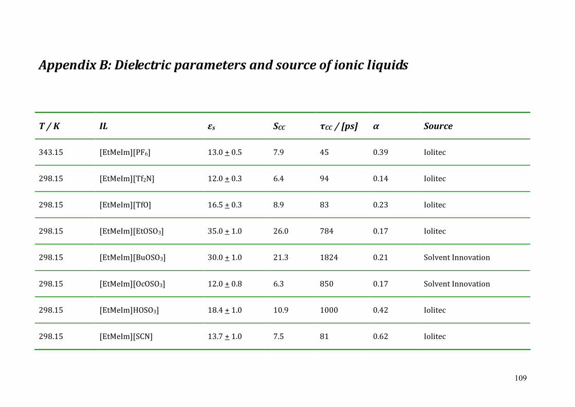
109
Appendix B: Dielectric parameters and source of ionic liquids
T / K IL εs SCC τCC / [ps] α Source
343.15 [EtMeIm][PF6] 13.0 + 0.5 7.9 45 0.39 Iolitec
298.15 [EtMeIm][Tf2N] 12.0 + 0.3 6.4 94 0.14 Iolitec
298.15 [EtMeIm][TfO] 16.5 + 0.3 8.9 83 0.23 Iolitec
298.15 [EtMeIm][EtOSO3] 35.0 + 1.0 26.0 784 0.17 Iolitec
298.15 [EtMeIm][BuOSO3] 30.0 + 1.0 21.3 1824 0.21 Solvent Innovation
298.15 [EtMeIm][OcOSO3] 12.0 + 0.8 6.3 850 0.17 Solvent Innovation
298.15 [EtMeIm]HOSO3] 18.4 + 1.0 10.9 1000 0.42 Iolitec
298.15 [EtMeIm][SCN] 13.7 + 1.0 7.5 81 0.62 Iolitec
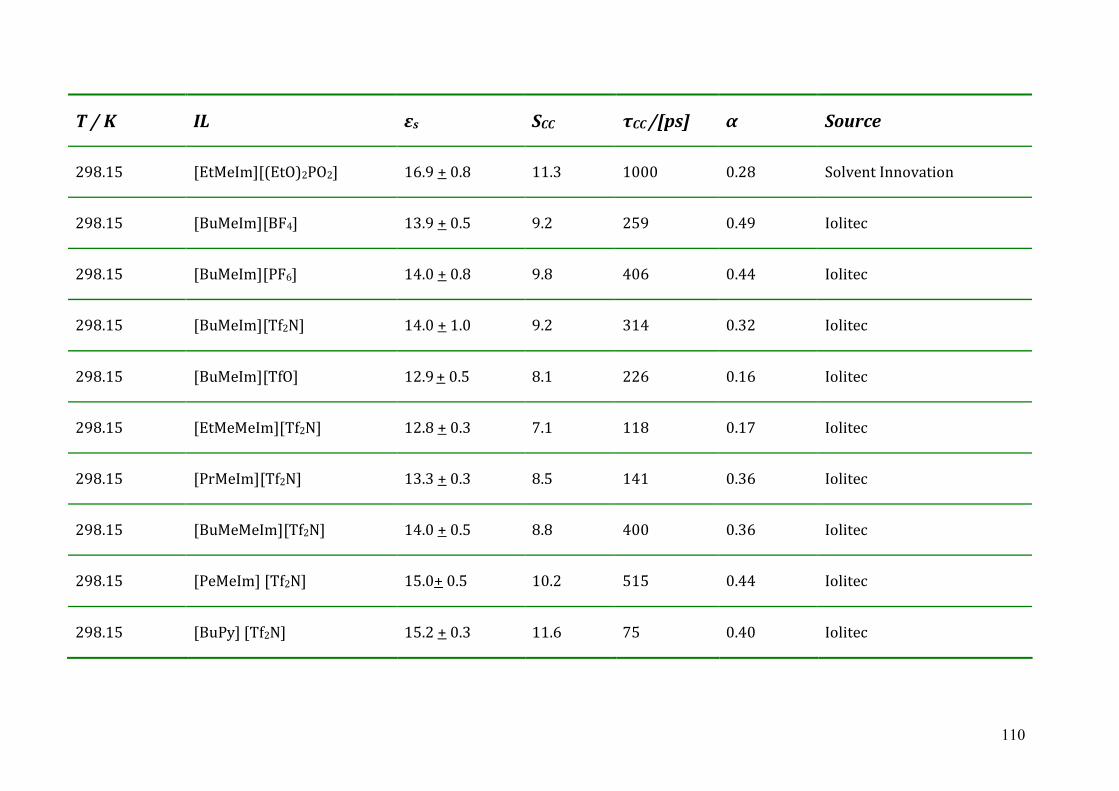
110
T / K IL εs SCC τCC /[ps] α Source
298.15 [EtMeIm][(EtO)2PO2] 16.9 + 0.8 11.3 1000 0.28 Solvent Innovation
298.15 [BuMeIm][BF4] 13.9 + 0.5 9.2 259 0.49 Iolitec
298.15 [BuMeIm][PF6] 14.0 + 0.8 9.8 406 0.44 Iolitec
298.15 [BuMeIm][Tf2N] 14.0 + 1.0 9.2 314 0.32 Iolitec
298.15 [BuMeIm][TfO] 12.9 + 0.5 8.1 226 0.16 Iolitec
298.15 [EtMeMeIm][Tf2N] 12.8 + 0.3 7.1 118 0.17 Iolitec
298.15 [PrMeIm][Tf2N] 13.3 + 0.3 8.5 141 0.36 Iolitec
298.15 [BuMeMeIm][Tf2N] 14.0 + 0.5 8.8 400 0.36 Iolitec
298.15 [PeMeIm] [Tf2N] 15.0+ 0.5 10.2 515 0.44 Iolitec
298.15 [BuPy] [Tf2N] 15.2 + 0.3 11.6 75 0.40 Iolitec
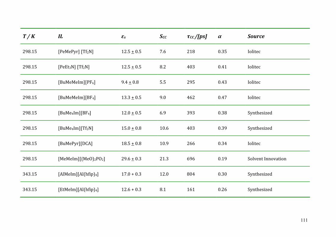
111
T / K IL εs SCC τCC /[ps] α Source
298.15 [PeMePyr] [Tf2N] 12.5 + 0.5 7.6 218 0.35 Iolitec
298.15 [PeEt3N] [Tf2N] 12.5 + 0.5 8.2 403 0.41 Iolitec
298.15 [BuMeMeIm][PF6] 9.4 + 0.8 5.5 295 0.43 Iolitec
298.15 [BuMeMeIm][BF4] 13.3 + 0.5 9.0 462 0.47 Iolitec
298.15 [BuMe4Im][BF4] 12.0 + 0.5 6.9 393 0.38 Synthesized
298.15 [BuMe4Im][Tf2N] 15.0 + 0.8 10.6 403 0.39 Synthesized
298.15 [BuMePyr][DCA] 18.5 + 0.8 10.9 266 0.34 Iolitec
298.15 [MeMeIm][(MeO)2PO2] 29.6 + 0.3 21.3 696 0.19 Solvent Innovation
343.15 [AlMeIm][Al(hfip)4] 17.0 + 0.3 12.0 804 0.30 Synthesized
343.15 [EtMeIm][Al(hfip)4] 12.6 + 0.3 8.1 161 0.26 Synthesized
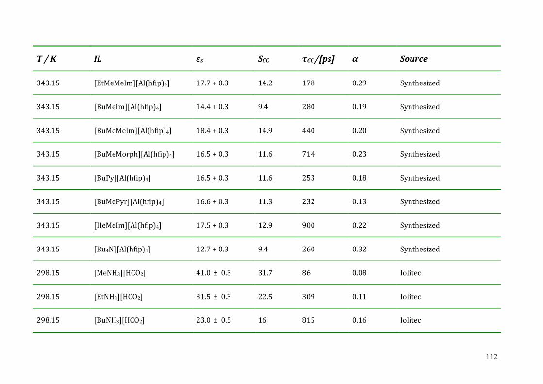
112
T / K IL εs SCC τCC /[ps] α Source
343.15 [EtMeMeIm][Al(hfip)4] 17.7 + 0.3 14.2 178 0.29 Synthesized
343.15 [BuMeIm][Al(hfip)4] 14.4 + 0.3 9.4 280 0.19 Synthesized
343.15 [BuMeMeIm][Al(hfip)4] 18.4 + 0.3 14.9 440 0.20 Synthesized
343.15 [BuMeMorph][Al(hfip)4] 16.5 + 0.3 11.6 714 0.23 Synthesized
343.15 [BuPy][Al(hfip)4] 16.5 + 0.3 11.6 253 0.18 Synthesized
343.15 [BuMePyr][Al(hfip)4] 16.6 + 0.3 11.3 232 0.13 Synthesized
343.15 [HeMeIm][Al(hfip)4] 17.5 + 0.3 12.9 900 0.22 Synthesized
343.15 [Bu4N][Al(hfip)4] 12.7 + 0.3 9.4 260 0.32 Synthesized
298.15 [MeNH3][HCO2] 41.0 0.3 31.7 86 0.08 Iolitec
298.15 [EtNH3][HCO2] 31.5 0.3 22.5 309 0.11 Iolitec
298.15 [BuNH3][HCO2] 23.0 0.5 16 815 0.16 Iolitec
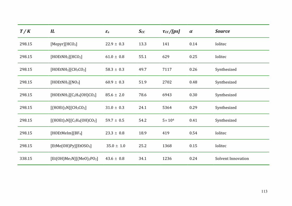
113
T / K IL εs SCC τCC /[ps] α Source
298.15 [Mepyr][HCO2] 22.9 0.3 13.3 141 0.14 Iolitec
298.15 [HOEtNH3][HCO2] 61.0 0.8 55.1 629 0.25 Iolitec
298.15 [HOEtNH3][CH3CO2] 58.3 0.3 49.7 7117 0.26 Synthesized
298.15 [HOEtNH3][NO3] 60.9 0.3 51.9 2702 0.48 Synthesized
298.15 [HOEtNH3][C2H4(OH)CO2] 85.6 2.0 78.6 6943 0.30 Synthesized
298.15 [(HOEt)3N][CH3CO2] 31.0 0.3 24.1 5364 0.29 Synthesized
298.15 [(HOEt)3N][C2H4(OH)CO2] 59.7 0.5 54.2 5104 0.41 Synthesized
298.15 [HOEtMeIm][BF4] 23.3 0.8 18.9 419 0.54 Iolitec
298.15 [EtMe(OH)Py][EtOSO3] 35.0 1.0 25.2 1368 0.15 Iolitec
338.15 [Et(OH)Me3N][(MeO)2PO2] 43.6 0.8 34.1 1236 0.24 Solvent Innovation
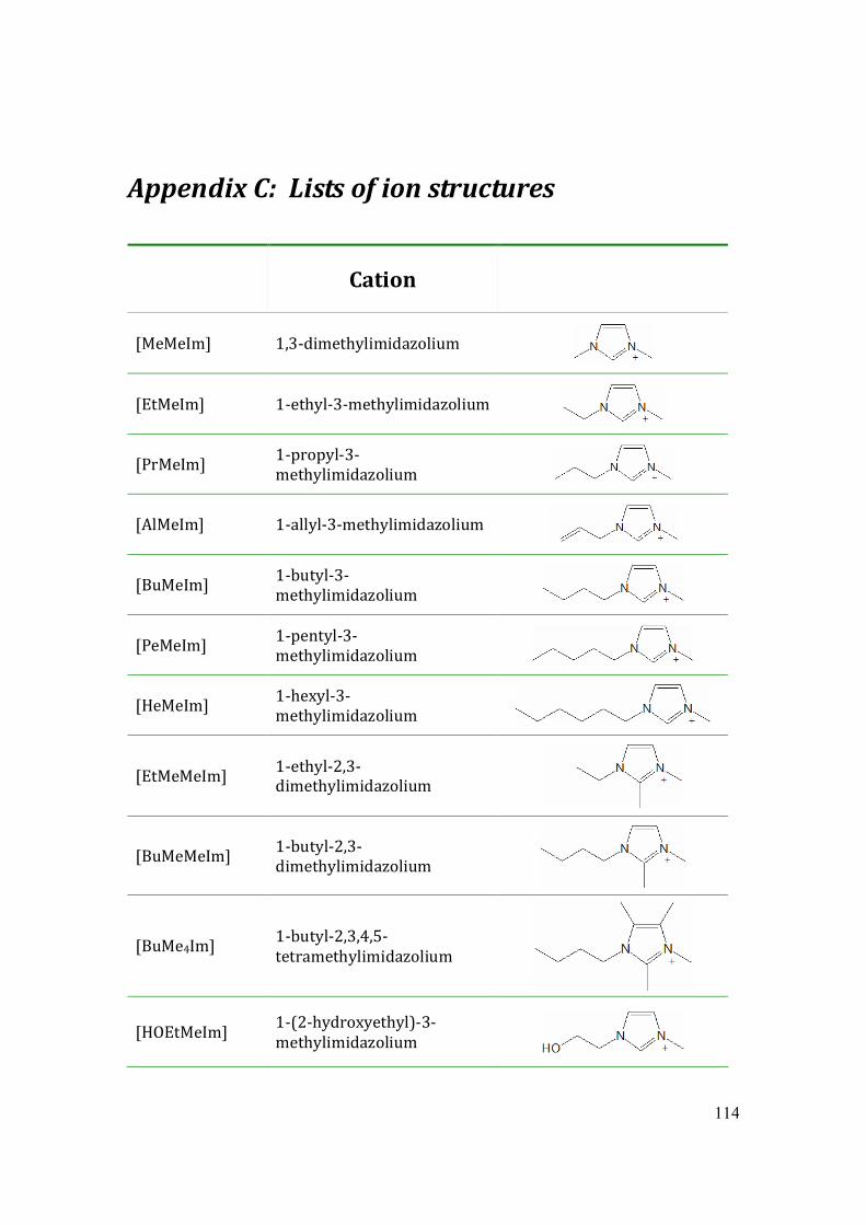
114
Appendix C: Lists of ion structures
Cation
[MeMeIm] 1,3-dimethylimidazolium
[EtMeIm] 1-ethyl-3-methylimidazolium
[PrMeIm] 1-propyl-3-methylimidazolium
[AlMeIm] 1-allyl-3-methylimidazolium
[BuMeIm] 1-butyl-3-methylimidazolium
[PeMeIm] 1-pentyl-3-methylimidazolium
[HeMeIm] 1-hexyl-3-methylimidazolium
[EtMeMeIm] 1-ethyl-2,3-dimethylimidazolium
[BuMeMeIm] 1-butyl-2,3-dimethylimidazolium
[BuMe4Im] 1-butyl-2,3,4,5-tetramethylimidazolium
[HOEtMeIm] 1-(2-hydroxyethyl)-3-methylimidazolium
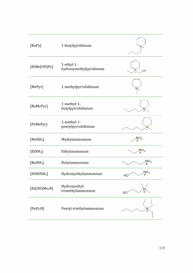
115
[BuPy] 1-butylpyridinium
[EtMe(OH)Py] 1-ethyl-1-hydroxymethylpyridinium
[MePyr] 1-methylpyrrolidinium
[BuMePyr] 1-methyl-1-butylpyrrolidinium
[PeMePyr] 1-methyl-1-pentylpyrrolidinium
[MeNH3] Methylammonium
[EtNH3] Ethylammonium
[BuNH3] Butylammonium
[HOEtNH3] Hydroxyethylammonium
[Et(OH)Me3N] Hydroxyethyl-trimethylammonium
[PeEt3N] Pentyl-triethylammonium
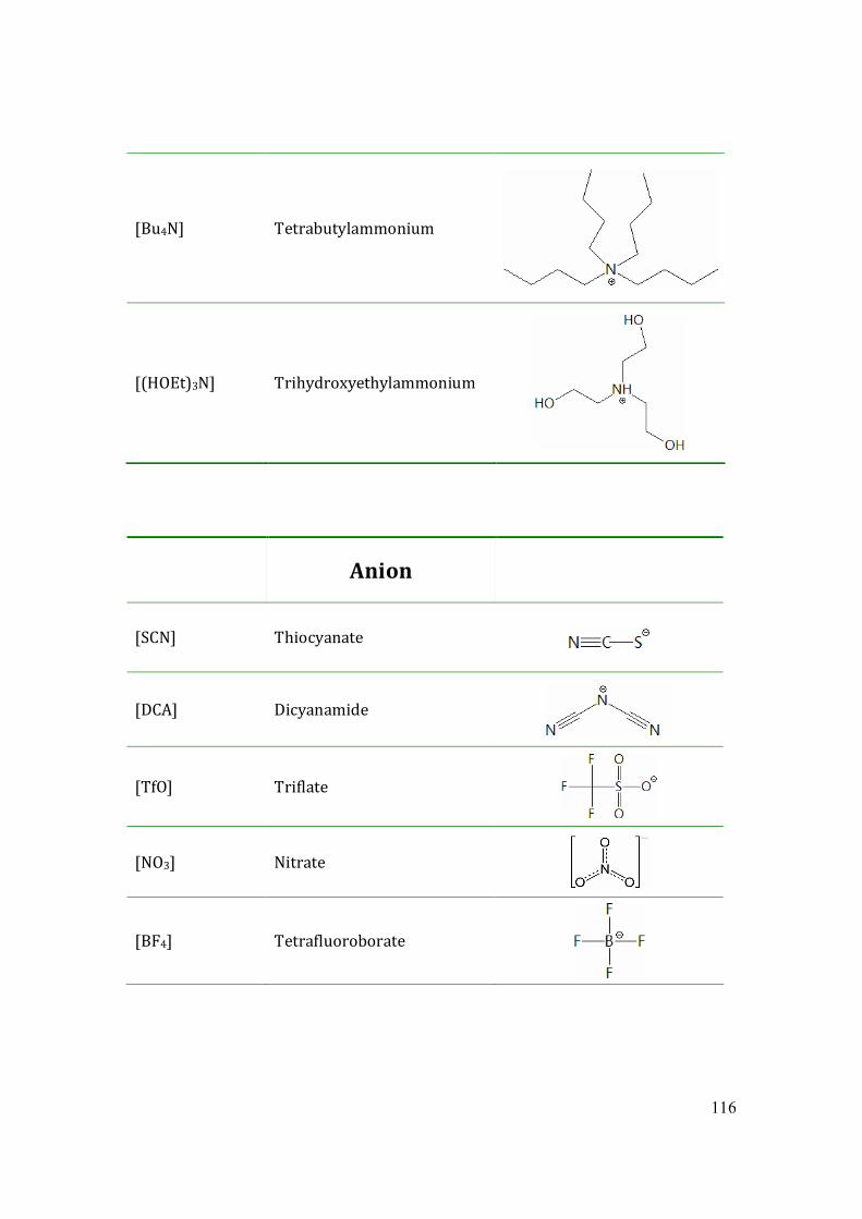
116
[Bu4N] Tetrabutylammonium
[(HOEt)3N] Trihydroxyethylammonium
Anion
[SCN] Thiocyanate
[DCA] Dicyanamide
[TfO] Triflate
[NO3] Nitrate
[BF4] Tetrafluoroborate
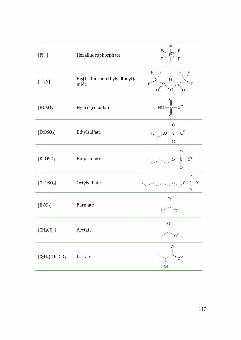
117
[PF6] Hexafluorophosphate
[Tf2N] Bis(trifluoromethylsulfonyl)imide
[HOSO3] Hydrogensulfate
[EtOSO3] Ethylsulfate
[BuOSO3] Butylsulfate
[OcOSO3] Octylsulfate
[HCO2] Formate
[CH3CO2] Acetate
[C2H4(OH)CO2] Lactate
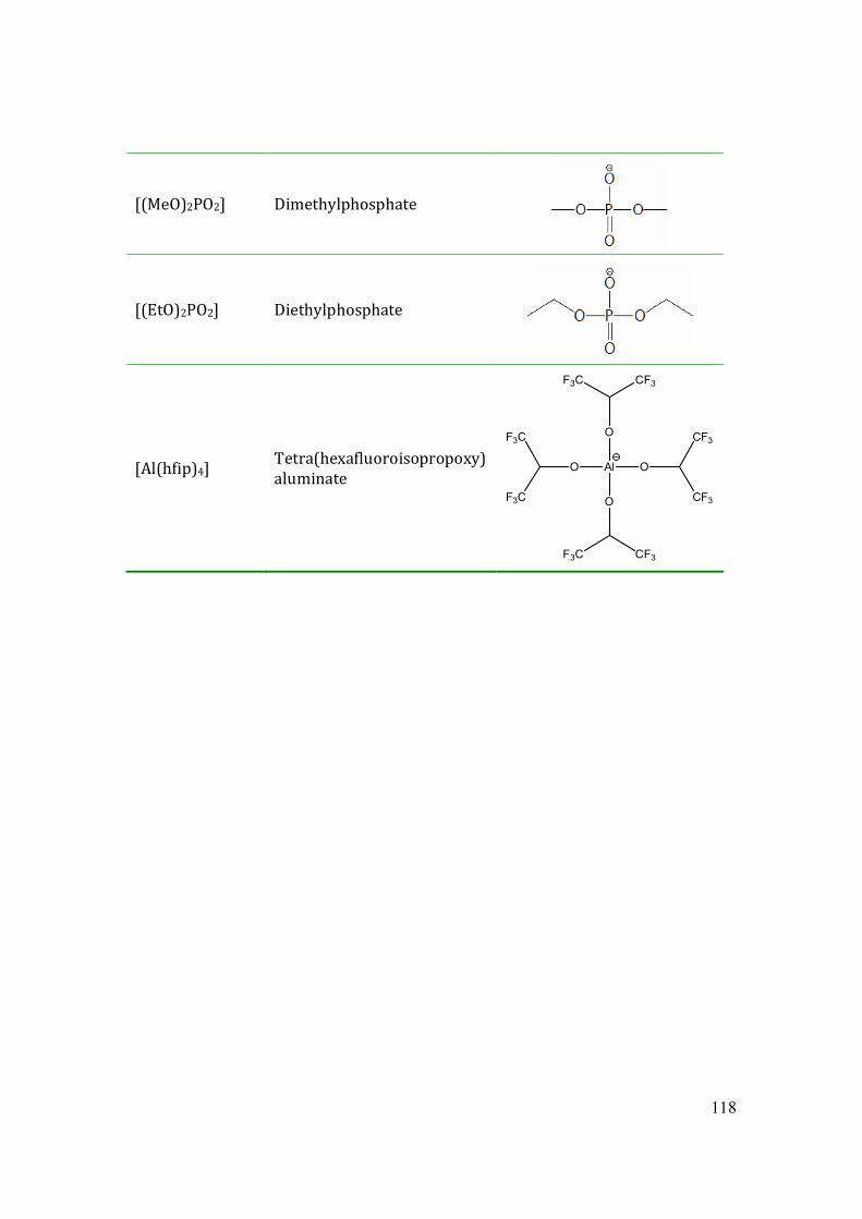
118
[(MeO)2PO2] Dimethylphosphate
[(EtO)2PO2] Diethylphosphate
[Al(hfip)4] Tetra(hexafluoroisopropoxy)aluminate
Al
O
O
O
O
CF3F3C
CF3F3C
F3C
F3C
CF3
CF3
119
Curriculum Vitae
Personal details Name: Mianmian Huang
Date of birth: 26.12.1978 in P.R.Chian, Fujian
Primary and secondary education 1985 – 1991 Primary School, China
1991 – 1997 Secondary School, China
Academic education 1997 - 2001 Bachelor of Science in Chemical Engineering
(Biotechnology)
Nanjing University of Science and Technology in China
2003 – 2005 Bachelor of Science in Chemistry,
Ruhr University Bochum
“Infrarotspektroskopische Untersuchung von
Van-der-Waals-Komplex ArCO”
2005 – 2006 Master of Science in Chemistry,
Ruhr University Bochum
“Dielektrische Spektroskopie an ionischen
Flüssigkeiten”
120
Research experience
2006 Research assistant, Physical Chemistry II,
Ruhr University Bochum
2006 – 2010 PhD studies in Physical chemistry,
Ruhr University Bochum
“Dielectric properties of ionic liquids”
Publications Huang, M. M. and H. Weingärtner
Protic Ionic Liquids with Unusually High Dielectric Permittivities.
ChemPhysChem. 2008 9(15): 2172-2173.
Mian-Mian Huang, Safak Bulut, Ingo Krossing, and Hermann Weingärtner
Communication: Are hydrodynamic models suited for describing the reorientational
dynamics of ions in ionic liquids? A case study of methylimidazolium
tetra(hexafluoroisopropoxy)aluminates
J. Chem. Phys. 133, 101101 (2010)
S. Bulut, P. Klose, M.-M. Huang, H. Weingärtner, P. J. Dyson, G. Laurenczy, C.
Friedrich, J. Menz, K. Kümmerer, and I. Krossing
Synthesis of Room Temperature Ionic Liquids with the weakly coordinating [Al(ORF)4]--
Anion (RF = C(H)(CF3)2) and the Determination of their Principal Physical Properties
Chem. Eur. J, 2010 online available
121
Mian-Mian Huang, Karola Schneiders, Peter S. Schulz, Peter Wasserscheid and Hermann
Weingärtner
Ion Speciation Driving Chirality Transfer in Imidazolium-based Camphorsulfonate Ionic
Liquids.
PCCP, online available DOI: 10.1039/c0cp01120g.
Mian-Mian Huang, Yanping Jiang, Padmanabhan Sasisanker, Gordon W. Driver,
Hermann Weingärtner
Static relative dielectric permittivities of ionic liquids at 25 oC
Submitted to Journal of Chemical and Engineering Data.