Embed Size (px)
Citation preview

Dielectric Properties and Space Charge Dynamics of Polymeric High
Voltage DC Insulating Materials


Dielectric Properties and Space Charge Dynamics of Polymeric High
Voltage DC Insulating Materials
Proefschrift
ter verkrijging van de graad van doctor aan de Technische Universiteit Delft,
op gezag van de Rector Magnificus prof. dr. ir. J. T. Fokkema, voorzitter van het College voor Promoties,
in het openbaar te verdedigen, op maandag 17 december 2007 om 17:30 uur
door
BELMA ALIJAGIĆ - JONUZ
elektrotechnisch ingenieur, geboren te Dubrovnik (Kroatië)
Dit proefschrift is goedgekeurd door de promotor: Prof. dr. J. J. Smit Samenstelling promotiecommissie: Rector Magnificus, Voorzitter Prof. dr. J. J. Smit, Technische Universiteit Delft, promotor Prof. dr. E. Ildstad, Norwegian University of Science Prof. dr. eng. J. A. Ferreira, Technische Universiteit Delft Prof. dr. ir. E. F. Steennis, Technische Universiteit Eindhoven Prof. dr. ir. J. van Turnhout, Technische Universiteit Delft Prof. ir. W. L. Kling, Technische Universiteit Delft/Eindhoven Dr. ir. P. H. F. Morshuis, Technische Universiteit Delft This research was funded by the listed companies: Philips Medical Systems, Hamburg Philips Medical Systems, Heerlen Philips Analytical, Almelo Philips FEI, Eindhoven Philips Components, Eindhoven Thales, Hengelo Tobias Jensen Capacitors, Lyngby PBF Electronics, Almelo ISBN 978-90-9022561-6 Copyright 2007 by Belma Alijagić – Jonuz Printined by PrintPartners Ipskamp, The Netherlands

Haastige spoed is zelden goed!
More haste, less speed!
Ko je žurio vrat je slomio!
Aan Edin Aan mijn ouders, Fatima en Fehim Jonuz

vii
TABLE OF CONTENTS TABLE OF CONTENTS…………………………………………. vii 1 INTRODUCTION 1.1 General………………………………………………………………. 1 1.2 Space charge measurements: state of the art………………………… 3 1.3 Aim of the thesis……...……………………………………………... 4 1.4 Outline of the thesis………………..………………………………... 5 2 EXPERIMENTAL 2.1 Introduction …………………………………………………………. 9 2.2 Test specimens………………………………………………………. 10 2.3 Pulsed electro-acoustic method……………………………………… 11
2.3.1 Description of the method…………………………………….. 11 2.3.2 Description of the equipment and measurement procedure…... 12
2.4 Polarization current measurement…………………………………… 15 2.4.1 Description of the method…………………………………….. 15 2.4.2 Description of the equipment and measurement procedure…… 15
2.5 Dielectric spectroscopy in the frequency domain……………………. 16 2.5.1 Description of the method…………………………………….. 16 2.5.2 Description of the equipment and measurement procedure…… 17
2.6 Breakdown tests……………………………………………………… 20 2.7 Electrical aging tests…………………………………………………. 20 3 THEORETICAL BACKGROUND 3.1 Introduction…………………………………………………………… 23 3.2 Space charge formation……………………………………………… 23 3.3 Conduction current…………………………………………………… 28 3.4 Dielectric polarization and relaxation………………………………… 29 4 THE EFFECT OF LONG-TERM DC STRESS ON
SPACE CHARGE DYNAMICS 4.1 Introduction…………………………………………………………… 35
viii
4.2 Charge dynamics of virgin and pre-stressed PC: results of the measurements…………………………………………… 41 4.2.1 Density, polarity and position of the accumulated space charge. 41 4.2.2 Electrical field strength………………………………………… 42 4.2.3 ρ vs. E characteristics and electrical threshold for space charge
accumulation………………………………………………….. 44 4.2.4 Space charge accumulation characteristic time……………….. 46
4.3 Charge dynamics of virgin and pre-stressed PC-TiO2: results of the measurements………………………………………………………… 48 4.3.1 Density, polarity and position of the accumulated space charge 48 4.3.2 Electrical field strength………………………………………… 49 4.3.3 ρ vs. E characteristics and electrical threshold for space charge
accumulation…………………………………………………... 51 4.3.4 Space charge accumulation characteristic time……………….. 53
4.4 Influence of TiO2 filler……………………………………………….. 54 4.5 Summary and conclusions…………………………………………… 56 5 RESULTS OF THE POLARISATION CURRENT
MEASUREMENTS 5.1 Introduction…………………………………………………………… 61 5.2 Polarisation and conduction currents in PC: results of the
measurements………………………………………………………… 62 5.3 Polarisation and conduction currents in PC-TiO2: results of the
measurements………………………………………………………… 65 5.4 Influence of TiO2 filler……………………………………………….. 67 5.5 Summary and conclusions…………………………………………… 67 6 MATERIAL CHARACTERIZATION BY
DIELECTRIC SPECTROSCOPY IN THE FREQUENCY DOMAIN
6.1 Introduction…………………………………………………………… 71 6.2 DSF on virgin and pre-stressed PC-TiO2: results of the measurements 75
6.2.1 Results of the tan δ measurements…………………………….. 74 6.2.2 Real part of complex permittivity……………………………... 85
6.3 DSF on virgin and pre-stressed PC: results of the measurements……. 86 6.3.1 Results of the tan δ measurements…………………………….. 86 6.3.2 Real part of complex permittivity……………………………... 93
6.4 Influence of TiO2 filler……………………………………………….. 94

ix
6.4 Summary and conclusions…………………………………………… 99 7 BREAKDOWN TESTS 7.1 Introduction…………………………………………………………... 101 7.2 Voltage endurance test and pre-stress determination…………………. 102 7.3 DC breakdown step-up tests…………………………………………. 103 7.4 Summary……………………………………………………………... 103 8 DISCUSSION OF THE RESULTS 8.1 Introduction…………………………………………………………... 107 8.2 Summary and discussion of the measurement results………………... 109
8.2.1 Space charge measurements…………………………………… 109 8.2.2 Polarization current measurements……………………………. 113 8.2.3 Dielectric spectroscopy in frequency domain…………………. 114 8.2.4 Breakdown tests……………………………………………….. 116
8.3 Conclusions of the discussion……………...…………………………. 117 8.3.1. Influence of TiO2 filler………………………………………… 117 8.3.2. Influence of pre-stressing……………………………………… 118 8.3.3. Conclusions……………………………………………………. 119
9 CONCLUSIONS AND RECOMENDATIONS 9.1 Introduction…………………………………………………………... 121 9.2 Conclusions…………………………………………………………… 122 9.3 Recommendations for the future work……………………………….. 125
APPENDICES Appendix A Practical case ……………………………………… 127 Appendix B Results of thermogravimetry ……………………….. 133 Appendix C Calculation of space charge ………………………… 137 Appendix D Charge accumulation ………………………………. 139 Appendix E Determination of the threshold field for space charge
accumulation ………………………..…………….. 143 Appendix F Polarization current fit …………………..………… 151 Appendix G Polarization current ……………………..………… 157

x
REFERENCES…………………………………………………...…… 161 LIST OF PUBLICATIONS …………………………………….. 169
SUMMARY…………………………………………………………… 171 SAMENVATTING………………………………………………….. 175 ACKNOWLEDGEMENTS………………………………….…… 179 CURRICULUM VITAE…………………………………………… 181

xi

xii
Introduction Chapter 1 1
IInnttrroodduuccttiioonn 11
1.1 General
The purpose of solid electrical insulating materials [1] is described as:
The purpose of electrical insulating materials is to isolate components of an electrical system from each other and from ground, while at the same time providing mechanical support to the component.
Nowadays, technology puts high demands on insulating materials with reductions in weight, dimensions, and production costs, and increases in reliability. In addition, insulating materials often have to meet other requirements, such as specific mechanical, thermal, or chemical properties. Consequently, finding a satisfactory compromise between economic demands and application dependent requirements becomes increasingly complex. To evaluate material applicability, an appropriate test method needs to be chosen. This selection process is one of the main subjects of this thesis. In addition, the research described in this thesis concentrates in particular on the determination

2 Chapter 1 Introduction
and analysis of the dielectric properties of insulating materials for DC driven applications. As a case study, polycarbonate was used, with and without the addition of TiO2 filler. Polycarbonate is frequently used in HVDC applications, in particular in X-ray applications (Appendix A). The basic idea behind the TiO2 filler addition was to reduce space charge accumulation, by increasing the materials’ ability of transportation of injected charge carriers. A test method may consist of one material test technique, or a combination of a number of material test techniques. Several material test techniques are available nowadays - destructive, non-destructive, applicable on-line or off-line - providing information about one or more material properties. Each of them has its advantages and disadvantages. For example, the advantage of some destructive techniques is that they often provide a quick answer about a material property. The great disadvantage is that the tested object cannot be used any more. As another example, the insulation condition of an electrical component that supports vital parts of some production process should be tested on-line; however, it might be easier and more favourable to use an off-line technique and to find a solution for temporary support of the vital parts of production, if possible. The current method under investigation comprises four test techniques: space charge measurements, conduction current measurements, dielectric spectroscopy in the frequency domain and breakdown testing. In the following, a brief overview is given of material properties, which are observed by the mentioned techniques. Space charge measurements The internal electrical field of an insulating material can be considerably modified by the presence of space charge. From the measured space charge profile, the distribution of the electric field is derived and as such, space charge measurements are a valuable tool to evaluate a dielectric which is to be used at DC voltage. The occurrence of space charge is often regarded as being detrimental; therefore, a relationship between space charge accumulation and electrical aging is expected. Space charge measurements provide us with a means to detect magnitude, polarity and location of charge trapped in a dielectric. In addition, different dielectrics can be compared regarding their tendency to accumulate charge. It appears that for many dielectrics a threshold field can be defined below which no or hardly any space charge accumulates. Conduction current measurements Space charge formation influences conduction mechanisms: the presence of space charge affects the conduction mechanism in the insulating material, and the conduction current-voltage characteristic is no longer linear, but it obeys a power law. Conduction current measurements allow us to identify a possible departure from ohmic conduction. Such a departure occurs when space charge
Introduction Chapter 1 3
starts to accumulate in a dielectric when the electric field is raised above a threshold level. Theoretical considerations show that this threshold level is quite close –if not identical– to the threshold for space charge accumulation. Dielectric spectroscopy in the frequency domain Dielectric changes in material structure can be detected by using dielectric spectroscopy over a wide frequency and temperature range. This technique completes the evaluation method for the characterisation of insulating materials, in particular with respect to aging. Breakdown testing Breakdown testing, usually involving step-up tests, is a frequently used insulation testing technique. However, it is very difficult and not completely correct to give a statement about the life expectancy of a polymeric material based on this test alone. The reason for this is that the classical step-up test does not take into account the time needed for space charge accumulation. On the other hand, if this time was taken into account, the test would become very time-consuming and, therefore, expensive. However, combining a breakdown test with some other less time-consuming characterisation techniques would be an appropriate alternative. Even better would be to find a relationship between the results of another characterisation technique and the voltage endurance of the material, which would then make the breakdown test redundant. In the next section we focused on the space charge phenomenon and its measurement technique, as being the youngest and least known of the four above mentioned test methods.
1.2 Space charge measurements: state of the art
The importance of intensive research into the phenomenon of space charge accumulation became obvious in the early 1980s with the application of high voltage DC cables in electrical energy transport due to their low dielectric losses over long distances in comparison with AC cables. However, the benefit of using DC is partially reduced by the damage that may be caused by space charge accumulation. The electric field in the insulation is enhanced due to the electric field of the accumulated space charge, and this enhancement may be high enough to accelerate electrical aging and even to initiate early insulation breakdown. Other high voltage DC applications - such as X-ray equipment, electron microscopes, image intensifiers, and radars - have also had to cope with the destructive effects of space charge accumulation on electrical insulation. More intensive research into the effects of space charge accumulation on electrical insulation materials started with the development of modern

4 Chapter 1 Introduction
measurement techniques, which use pulse excitation for interaction with accumulated space charge in order to localise and measure it. In most cases, a material specimen is placed in a plane capacitor configuration and charged with a DC voltage, thereby generating space charge in the material. The TSP (thermal step pulse) method [2] uses a temperature step for the displacement of space charge. LIPP (laser induced pressure pulse), PWP (pressure wave propagation), and PPP (piezoelectrically generated pressure pulse) all use the displacement of the space charge pressure pulse that travels as an acoustic wave through the material [3-6]. As a consequence of space charge displacement, the electrode charges change, resulting in an electrical signal in the external circuit of the measuring systems. The PEA (pulsed electro-acoustical) method [5], [7-12] uses short electrical pulses which interact with space charge, and result in an acoustic wave whose intensity and time delay correspond to space charge density and position. Initially, the most common methods used for space charge observation were destructive methods like the field mill and the capacitive probe [13]. Most of the research on space charge accumulation in electrical power engineering has been performed on polyethylene (PE) based materials, which are used in high voltage AC and DC cables [14-20]. There are fewer examples of research on other insulating materials: the most commonly cited are epoxy with or without filler [21-22], impregnated paper [23], polycarbonate with and without filler [24], and PMMA [25]. It has been experimentally proven for PE-based materials that space charge can be considered as one of the causes of failure [26-27]; as already mentioned, electric field enhancement due to space charge accumulation can have deleterious effects on insulation materials. In this sense, it is suitable as a parameter for material testing and ranking. Space charge can also be considered as a consequence [28-29] of electrical aging: the number and distribution of trapping sites where space charge can be captured changes due to electrical aging. The physical processes behind space charge accumulation are quite complex and still not fully understood. There are few physical models for space charge accumulation available, all of which have certain discrepancies when compared with experimental results, some of them even without experimental evidence [30-34]. More successful are phenomenological models made mainly for PE-based materials, but they are also far from universal [35-39].

Introduction Chapter 1 5
1.3 Aim of the thesis
The aim of the here described research was twofold: To establish a method to estimate the (future) performance of polymeric
insulating materials for DC driven applications. To evaluate experimentally the dielectric properties of polymeric
insulating materials relevant for normal operating conditions in high voltage DC applications.
The following approach was adopted: As a case study, polycarbonate was used, with and without the addition of TiO2 filler. The specimens were tested when virgin, and after long-term stress at high DC fields. Four test techniques were combined:
Breakdown tests (voltage endurance tests) Space charge measurements Polarization current measurements Dielectric spectroscopy in the frequency domain
1.4 Outline of the thesis
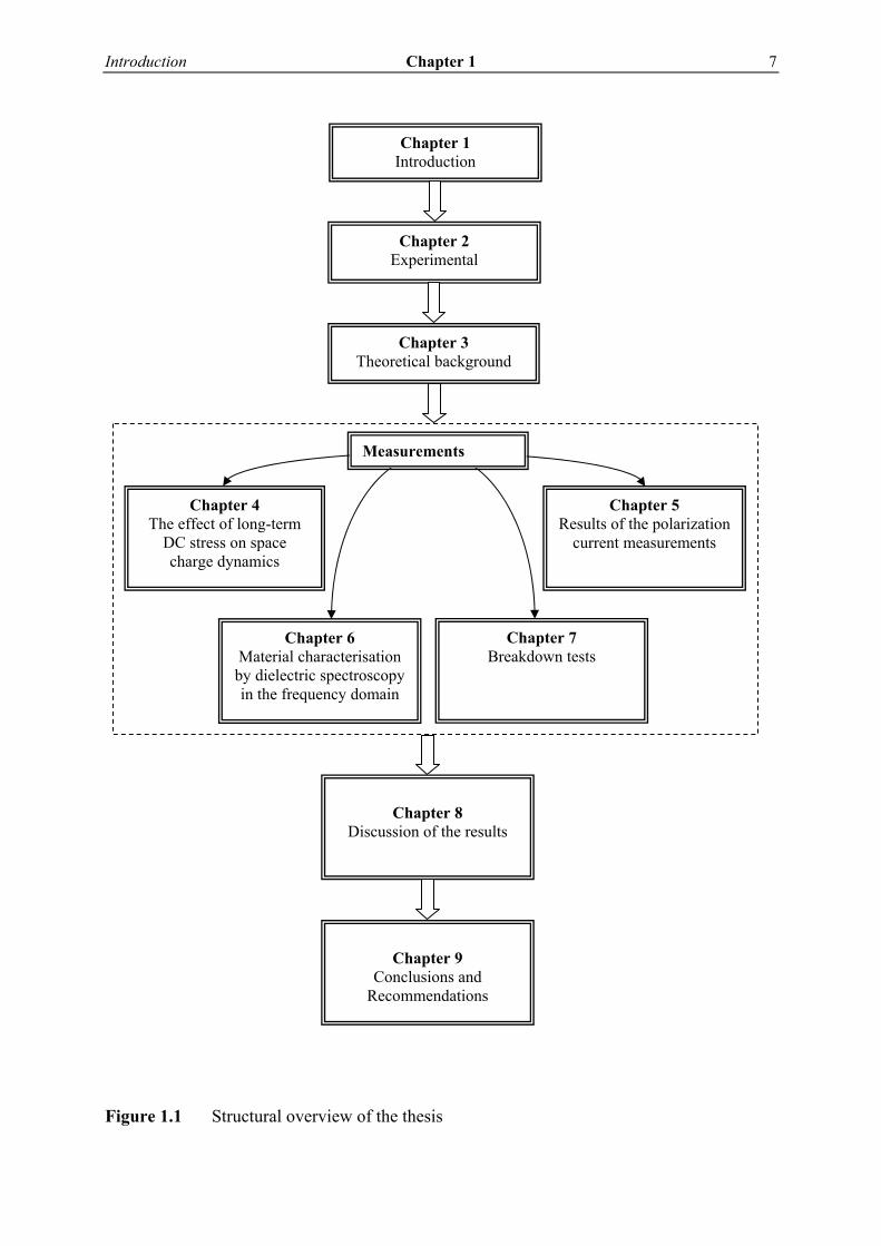
The structural overview of the thesis is given in Figure 1.1. Chapter 2 describes the technical basis of the four mentioned characterisation techniques. Chapter 3 covers the physical background and an analytical description of space charge phenomena, conduction current analysis, and dielectric spectroscopy in the frequency domain. The description of the main processes behind the breakdown of insulating materials is assumed to be well-known, and is therefore not repeated. An excellent description can be found in [40-41]. In Chapters 4-7, the experimental results are presented and discussed. Experimental investigation was carried out on virgin and pre-stressed PC and PC-TiO2 specimens. Chapter 4 presents the results of space charge measurements performed in order to establish the space charge dynamics of PC and PC-TiO2, and to analyse the effect of long-term exposure to a high electric DC field on the space charge behaviour of the materials. Based on the space charge measurements, the following space charge related quantities were calculated and derived: space charge density, polarity and position; electrical field strength and field enhancement factor; space charge accumulation characteristic times; and the electrical threshold for space charge accumulation, Eth,sc. Results of the polarisation current measurements are shown in Chapter 5. The steady-state values of the polarisation currents - the conduction currents - were plotted against applied electric fields with the objective of investigating

6 Chapter 1 Introduction
whether the examined materials show the presence of an electric threshold at which a transition between different conduction mechanisms takes place. The effects of electrical stress on the materials and the influence of TiO2 filler were also explored. Measurement results of tan δ and the real part of complex permittivity, performed by means of dielectric spectroscopy in the frequency domain are presented in Chapter 6. The objective of the chapter is to probe the dielectric relaxation processes in the tested materials, to explore the effects of electrical stress, and to establish the influence of TiO2 filler on molecular dynamics. The voltage endurance of new and pre-stressed materials is determined by means of step-up tests as described in Chapter 7. In Chapter 8, the results of the measurements are discussed in light of the main objective: to arrive at a classification method that evaluates the DC performance of polymeric insulating materials. Conclusions and recommendations for future work are given in Chapter 9.
Introduction Chapter 1 7
Figure 1.1 Structural overview of the thesis
Chapter 1 Introduction
Chapter 2 Experimental
Chapter 3 Theoretical background
Chapter 4 The effect of long-term
DC stress on space charge dynamics
Chapter 5 Results of the polarization
current measurements
Chapter 6 Material characterisation by dielectric spectroscopy in the frequency domain
Chapter 7 Breakdown tests
Chapter 8
Discussion of the results
Chapter 9
Conclusions and Recommendations
Measurements

8 Chapter 1 Introduction
Experimental methods Chapter 2 9
EExxppeerriimmeennttaall mmeetthhooddss 22
2.1 Introduction
In this chapter, a description is given of the specimens, material test techniques, and measuring set-ups used in this work. Section 2.2 contains the specimens’ specifications, and details of the specimen treatment procedures that were employed prior to measurements being taken. Sections 2.3 - 2.5 give a description of the following material test techniques:
Pulsed electro-acoustic measurements, used for space charge measurements. Dielectric spectroscopy in the frequency domain used for tan δ and complex
permittivity measurements. Polarization current measurements, used for the determination of electric
field-conduction current characteristics. The mentioned test techniques were applied to virgin and pre-stressed PC and PC-TiO2 with the objective of analyzing the following aspects:
Material performance concerning the following measured/calculated quantities:
10 Chapter 2 Experimental methods
- Space charge related quantities - Dielectric relaxations, complex permittivity - Conduction current; transition field from linear to non-linear regime - Breakdown strength
Influence of 100 kV/mm DC - 1500 hours pre-stressing on above mentioned material parameters.
Influence of the addition of TiO2 on polycarbonate dielectric properties. Section 2.6 describes the breakdown tests used for the determination of the electrical pre-stress field, which should be high enough to trigger material deterioration but at the same time low enough not to cause material breakdown. Section 2.7 gives a description of the electrical aging test.
2.2 Test specimens
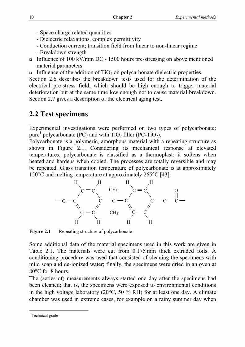
Experimental investigations were performed on two types of polycarbonate: pure1 polycarbonate (PC) and with TiO2 filler (PC-TiO2). Polycarbonate is a polymeric, amorphous material with a repeating structure as shown in Figure 2.1. Considering its mechanical response at elevated temperatures, polycarbonate is classified as a thermoplast: it softens when heated and hardens when cooled. The processes are totally reversible and may be repeated. Glass transition temperature of polycarbonate is at approximately 150°C and melting temperature at approximately 265°C [43].
Figure 2.1 Repeating structure of polycarbonate Some additional data of the material specimens used in this work are given in Table 2.1. The materials were cut from 0.175 mm thick extruded foils. A conditioning procedure was used that consisted of cleaning the specimens with mild soap and de-ionized water; finally, the specimens were dried in an oven at 80°C for 8 hours. The (series of) measurements always started one day after the specimens had been cleaned; that is, the specimens were exposed to environmental conditions in the high voltage laboratory (20°C, 50 % RH) for at least one day. A climate chamber was used in extreme cases, for example on a rainy summer day when
1 Technical grade
C
H
H
H
H
O
O C
CH3
CH3
O C C
C C
C C
H
H
H
H
C C
C C
C C
Experimental methods Chapter 2 11
the temperature and humidity in the high voltage laboratory were very difficult to control and could reach values of 25°C and 80 % RH. Table 2.1 Specimens’ specification Material
Filler type and content Thickness [mm] Relative
permittivity εr Glass transition temperature Tg
PC none 0.175 3.1 155°C PC-TiO2 TiO2 16.7 % wt 0.175 3.7 155°C Specimens used for space charge measurements and dielectric spectroscopy measurements were always space charge free. Discharging of charged specimens was brought about by short-circuit and, if necessary, by heating the specimens at 80°C for a couple of days. In extreme cases the specimens were heated at 150°C for a short period of time. Specimens that spent some period in insulating oil (for the purposes of electrical-aging tests) were cleaned in the same way. According to Thermogravimetric Analysis (TGA) and dielectric spectroscopy measurements, no detectable amount of oil had penetrated the specimens; therefore, no special cleaning procedure was applied. The results of TGA and dielectric spectroscopy measurements are shown in Appendix B.
2.3 Pulsed electro-acoustic method
2.3.1 Description of the method
A material specimen is put between two electrodes, El1 and El2, as shown in Figure 2.2 ([7]-[12], [15], [23], [24]). Given a charge-free specimen, the application of DC voltage (generated by source UDC) causes surface charge densities σ1 and σ2 on the electrodes and a volume charge density ρ in the material specimen. During a measurement, a very short, high voltage pulse is applied, generated by a pulse source. When this electric pulse is present, the resulting electric field acts on the space charge inside the material. Due to this field, the space charge and charge at the electrodes experience an electrostatic force, F. The force is of short duration and, as a result, two acoustic waves propagate in both directions, to El1 and El2. The wave traveling in the direction of El2 is initially transferred to the electrode material, which acts as a delay block for the acoustic wave until its arrival at a piezoelectric sensor/transducer. The delay is necessary because of the interference of the electromagnetic noise caused by the ignition of the electrical pulse. The piezoelectric transducer detects the acoustic wave and transforms it into an electric signal. The signal is fed into an oscilloscope, and from there into a computer. The computer stores the signal and performs some signal shaping and calibration. The wave in the direction of El1 is first reflected at El1 and then follows the same acoustic path, as previously described.

12 Chapter 2 Experimental methods
Figure 2.2 Principle of PEA measurement The result of a PEA measurement is an electrical, time-dependent signal, u(t). The signal is made space-dependent using a well known relationship between path s[m], velocity υsound [m/s] and time t [s], s = υsound⋅ t. The measured voltage signal, u in mV, is converted to a charge signal ρ in C/m3 according to relation (2.1).
(2.1)
where Kcal is the calibration factor. The calibration factor can be calculated as (2.2) from a known charge, which is in this case the surface electrode charge. A slab of charge [C/m3] is a product of a surface charge σ [C/m2] and the slab thickness b [m], ρ = σ/b. For a detailed description see Appendix C and [23].
( )specimencal
specimencalcal U
bdtuK
ε= (2.2)
where: ucal(t) is signal measured during the calibration measurement, dspecimen is the thickness of the material specimen, εspecimen is the permittivity of the material and Ucal is the DC voltage during the calibration.
2.3.2 Description of the equipment and measurement procedure
Equipment The equipment used for PEA measurements in this thesis consisted of:
Electrodes HV: stainless steel covered with semi-con rubber; LV: aluminum 18 mm, also used as a delay block. A droplet of oil was interposed between the electrodes and the test specimen, to improve acoustical coupling.
Charging DC supply: Heinzinger 40 kV, 15 mA Pulse DC supply: Heinzinger 10 kV, 5 mA Pulse width 6 ns
oscillo-scope
____
ρ F
σ1 σ2
El1 El2
C
R
UP
UDC
PVDF backing material
A computer
uK
ρcal
1=

Experimental methods Chapter 2 13
Spatial resolution Between 13 μm and 17 μm; calculated as: r = υ⋅ ΔT Where r is the spatial resolution,υ [m/s] is the sound velocity in the material, ΔT is the pulse width.
Sensor/transducer Bi-oriented PVDF foil, 9 μm Amplifier Two 23 dB amplifiers, bandwidth 0.1 – 500 MHz Oscilloscope Digital storage 2 GSa/s, HP 54522 A
The high voltage DC circuit and the signal detection circuit are completely separated in the PEA method. Therefore, the output signal is shielded easily and less electric noise enters the detection circuit. Also, the risk of damaging the detection circuit in the event of specimen breakdown is minimal. The measuring set-up, was placed in an EMC shielded space. A personal computer with a GPIB interface was used for displaying and storing of measured data. Measurement procedure There are two possible ways to perform a space charge measurement: a voltage-on or a voltage-off measurement, Figure 2.3. The time-dependent voltage signal u(t) [mV], recorded by the oscilloscope, is called the space charge profile. Space charge density is calculated from this signal (Appendix C). The average space charge density present in the test specimen is calculated from this signal according to the following relationship:
dxρ(x)d
ρd
avg ∫=0
1 (2.3)
Voltage-on measurement During a voltage-on measurement, a poling voltage is applied to the test specimen allowing space charge to accumulate. A difficulty with this way is that due to limited spatial resolution and the non-rectangularity of the high-voltage pulse [23], the signals originating from the electrode charges and the signal originating from the space charge may overlap, Figure 2.4.
Voltage-off measurement To reduce the effect of the electrode charges, a voltage-off measurement is performed: in this case the poling voltage is switched off, the electrode charges’ signals disappear, and on the screen of the oscilloscope the only visible signals are the signals originating from the accumulated space charge and mirror charges at the electrodes.
Sometimes we are interested in measuring the amount of space charge already present in a material prior to poling, for example, as a consequence of electrical aging. In such a case, only a voltage-off measurement is performed. The duration of a voltage-on measurement is chosen such that the charging process of the test specimen is completed within the duration of the test. Materials used in this thesis showed no considerable changes of accumulated space charge when charged for longer than 3 hours.

14 Chapter 2 Experimental methods
The duration of a voltage-off measurement depends on its purpose. For the calculation of accumulated space charge, the measurement takes 10 s. To observe the complete process of the discharging of the test specimen can take days.
Figure 2.3 An example of a voltage-on and voltage-off space charge measurement in
epoxy [44]: a) Voltage-on measurement at time t = 0. b) Voltage-on measurement at time t = 3 hours. It is not possible to identify a
difference between electrode charges and space charge at time t = 3 hours in the voltage-on measurement.
c) Voltage-off measurement immediately after switching off the charging voltage. Space charge is clearly visible in the voltage-off measurements.
0.5-12 ch
arge
den
sity
[µC
/cm
3 ]
-8
-4
0
4
8
voltage-on time = 0
0 specimen thickness [mm]
-8
-4
0
4
8
char
ge d
ensi
ty [µ
C/c
m3 ]
voltage-on time = 3h
-12 0.50
specimen thickness [mm]
0.5
-4
0
4
8
voltage-off time = 3h
0
char
ge d
ensi
ty [µ
C/c
m3 ]
Detected space charge
specimen thickness [mm]
LV electrode HV electrode

Experimental methods Chapter 2 15
Accuracy of the PEA measurements The accuracy of the PEA measured space charge value in this work is approximated to be 15 %. According to [15, 23], two most relevant factors affecting the accuracy of PEA measurements are: the systematic error of the calibration procedure and the statistical error due to the presence of noise in detected signal. In [23] the error is found to account for 12 %, while the statistical error contributes 1 % to 3 % to the total relative error. As the same measurement procedure and data processing were adopted in this work, as well as quite similar equipment, it is assumed that the total relative error also in this case will not exceed 15 %.
2.4 Polarization current measurement
2.4.1 Description of the method
The polarization current measurement is performed by applying a DC voltage to material placed in a parallel plane electrode configuration, Figure 2.4. The polarization processes are thereby started and a small polarization current can be measured. The polarization current has a decreasing character and when all polarization processes are finished only the small conduction current remains.
Figure 2.4 Measurement principle of the polarization current.
2.4.2 Description of the equipment and measurement procedure
Equipment The experimental set-up used for measurements of polarization current is shown in Figure 2.5. The used equipment is specified below.
Electrodes High voltage: Rogowski-profiled aluminum electrode Covered with 1 mm semicon rubber Low voltage: aluminum, guarded
Charging DC Heinzinger, 40 kV, 15 mA Electrometer Keithley 617, programmable electrometer, bipolar 100 V
source, accuracy 0.05 %, connected to the measuring electrode via 10 MΩ resistor.
electrometer
test specimen DC =
i(t) polarization current
time
conduction current a.
u.
a.u.

16 Chapter 2 Experimental methods
The measuring set-up was placed in an EMC shielded cage. A personal computer with a GPIB interface was used for displaying and storing of measured data.
Figure 2.5 Experimental set-up used for measurements of polarization current Measurement procedure For the polarization current measurement, a poling voltage is applied to the test specimen for at least 10000 s to make sure that the polarization processes are finished and that the only current which is measured is the conduction current. The polarization current is automatically recorded by a computer. All polarization current measurements reported in this thesis were performed at ambient temperature. Accuracy of the measurements The accuracy of the polarization current measurements in this work is approximated to be 12 %. The error of the measurements caused by uncertainty in DC voltage and dimensions of the test specimens is calculated to be 10 %. Statistical error of 2 % has its origin in the presence of noise, which is introduced in amplifiers and signal cables.
2.5 Dielectric spectroscopy in the frequency domain
2.5.1 Description of the method
Dielectric spectroscopy in the frequency domain makes use of the fact that each dielectric mechanism has a characteristic relaxation frequency or frequency band. For the purposes of dielectric spectroscopy, a time dependent electric field is used to probe molecular dynamics and charge transport. Reorientation (or relaxation) of dipolar groups, electronic or ionic conductivity, as well as induced polarization processes contribute to relative complex permittivity iε ε ε′ ′′= − .
electrometer
R GPIB interface
PC, data display and storage
HVDC HV electrode Semicon rubber
Guarding electrodeTest specimen
∼ ∼

Experimental methods Chapter 2 17
The complex permittivity can be calculated from the complex impedance measurement, the principle of which is given in Figure 2.6 [45].
Figure 2.6 Principle of a dielectric measurement using a frequency response analyzer. The sample material with complex permittivity ε(ω) is placed in a parallel plate capacitor configuration. The AC voltage U with the frequency of measurement f is applied to the sample capacitor by the generator. The resistor R converts the sample current I into voltage. The amplitude and the phase of U and I are measured by two phase sensitive voltmeters.
IUZ = (2.4)
Where Z denotes the impedance of the sample capacitor. Neglecting edge effects, complex permittivity is obtained from the standard equation of a parallel plate capacitor:
AεdCiεε0
=′′−′= ε (2.5)
where d is the distance between the plates, A is the area of one of the plates, ε0 is the vacuum permittivity and C is sample capacitance calculated from measured impedance.
2.5.2 Description of the equipment and measurement procedure
Equipment For the dielectric spectroscopy measurements in the frequency domain a modular measurement system made by Novocontrol was used. The equipment consisted of:
Impedance analyzer: frequency range 3 μHz to 20 MHz, impedance 10-2 Ω to 1014 Ω, accuracy tan δ ≈ 1·10-5
Cryostat: temperature range -160°C to 400°C, sensitivity of temperature controller ± 0.01 K
Temperature control: liquid nitrogen and 4-channel temperature controller Specimen holder, see Figure 2.8
Voltage source ≈
R
Specimen
I
U

18 Chapter 2 Experimental methods
For frequencies above 1 MHz [46], the sample impedance may become in the same order as the inductive impedance of the BNC cables connecting the specimen holder with the analyzer. This limits the measurements to frequencies below approximately 3 MHz. For high impedance test specimens, long cables cause additional problems due to the electrical noise created by mechanical vibrations. Therefore, cable length should be kept as short as possible. This is achieved by placing the complete analogue electronics at the top of the specimen holder, but not in the impedance analyzer. The connection to the electrodes of the specimen holder is done with solid air insulated lines that have only a tenth of the inductivity of 1 meter of BNC cable, see Figure 2.8. Depending on the test specimen temperature set point, a heating element builds up a specified pressure in the liquid nitrogen Dewar vessel in order to create a highly constant nitrogen gas flow, Figure 2.7. The pressure and temperature in the Dewar are measured by two of the temperature controller’s channels.
Figure 2.7 Specimen cell and cryostat temperature control.
After being heated by a gas jet, nitrogen gas flows directly through a sample cell that is mounted in a cryostat. The gas and sample temperature are measured by the two remaining channels of the temperature controller. The cryostat is vacuum isolated by a 2-stage rotary vane vacuum pump, providing thermal isolation by low vacuum (< 10 µbar). All temperature experiments are supported by the Novocontrol software package, providing both isothermal control and temperature ramping.
Sample cell
Cryostat
N2 outlet
Vacuum pump Vacuum gauge
Dewar
PT 100 temperature sensor
Dewar temperature sensor Liquid nitrogen evaporator
Gas heating module
Pressure sensor
Ch. 3
Ch. 2
Ch. 1
Ch. 4
Temperature controller
Dewar Gas heater Gas temperature sensor

Experimental methods Chapter 2 19
Measurement procedure For dielectric spectroscopy in the frequency domain only metallised specimens were used. The measurements reported in this thesis were recorded across broad temperature and frequency ranges. The duration of most measurements was from 5 to 12 hours. The applied voltage was 3 V. Prior to each measurement, the test specimen’s temperature was kept at 20°C for approximately 15 minutes in order to achieve thermal equilibrium between the test specimen and the electrodes of the specimen holder. After the temperature stabilization, the measurements were performed in three temperature runs. In this way, tension in the material or a preference direction2 of polarizable parts was removed.
Figure 2.8 Active specimen holder.
2 A preference direction can be a consequence of long-term exposure to high DC voltages or a consequence of the manufacturing process.
GEN V1 V2 PT100
Impedance analyser connector
PT 100 connector
Sample mounting screw
Electrode connectors
PT 100 temperature sensor
Upper electrode, current sense
Lower electrode, AC signal source
Upper electrode signal
Lower electrode signal
Input for voltage amplifier in the cell head

20 Chapter 2 Experimental methods
2.6 Breakdown tests
The breakdown tests were done by increasing the poling voltage in steps until breakdown occurred. The same set-up as for the electrical aging test was used, Figure 2.9. At least four specimens of each material used in this thesis were tested. The mode of increase of the voltage was 2 kV/minute. As the start, the voltage was set at 40 % of the probable short-time breakdown voltage. The probable short-time breakdown voltage was obtained in accordance with the following method:
The voltage was raised from zero at a uniform rate until breakdown occurred. The rate of rise that most commonly caused breakdown to occur within 60
seconds was selected. If breakdown occurred in less than six levels from the start of the test, a further four specimens were tested using a lower starting voltage. The electric strength was based on the highest nominal voltage that was withstood for 60 s without breakdown.
2.7 Electrical aging tests
The electrical aging tests were carried out by submerging the test specimens in a vessel filled with mineral insulating oil, type Shell Diala B. The specimens were placed between two stainless steel electrodes in the specimen holder shown in Figure 2.9. Sixteen specimen holders can be used at the same time in the aging set-up.
Figure 2.9 Specimen holder for aging and breakdown test set-ups.
Breakdown detection
Stainless steel
Teflon
Test specimen
Experimental methods Chapter 2 21
The specimen holders were connected to a breakdown detection circuit that provided information about the breakdown time and automatically switched off the voltage supply in the event of breakdown. The poling voltage was supplied by a Heinzinger high voltage DC source with a maximum voltage output of 150 kV and a maximum current output of 50 mA. The duration of the test was 1500 hours. The applied electric field was 100 kV/mm.

22 Chapter 2 Experimental methods
Theoretical background Chapter 3 23
TThheeoorreettiiccaall bbaacckkggrroouunndd 33
3.1 Introduction
In the following section, an overview is given of the main processes whose parameters are measured by means of: space charge measurements, polarisation current measurements, and dielectric spectroscopy in frequency domain. Thereby a physical background is explained and an analytical description is given. The description of the main processes behind the breakdown of insulating materials is assumed to be well known, and is therefore not covered. An excellent description can be found in [40-41].
3.2 Space charge formation
Space charge accumulates when the flow of charge carriers into a region of space differs from the out-flow from that region [47]. Several physical mechanisms are involved in space charge formation: charge injection/extraction, transportation, trapping, recombination, and carrier generation. Thereby, the
24 Chapter 3 Theoretical background
generation of space charge is expressed by the current continuity law, in (3.1) given in 1-dimensional form:
( ) ( ) txρ
xxJ 0
dd =
∂∂+ (3.1)
where J represents the current density and ρ the space charge density in point x. In other words, any situation where the current density J differs in space, dJ(x)/dx ≠ 0, will lead to the generation of space charge. The divergence of the current density is found at various places: at an electrode-dielectric interface, at a dielectric-dielectric interface, in the presence of a temperature gradient, in material in-homogeneity, and in a diverging field. Electrode-dielectric interface Considering the electrode-dielectric interface, the build-up of space charge depends on the difference between the flow of the charge carriers through the interface (injection/extraction), and the flow of the charge carriers through the material (transportation). If the flow through the interface equals the flow through the material, there will be no space charge formation. In cases where the injection/extraction rate of the charge carriers is higher than the transportation rate, space charge will primarily build-up in the vicinity of the electrodes. The charge polarity is, in this case, the same as the electrode polarity and this charge is denoted as a homo-charge. The electrical field due to the homo-charge decreases the electrode field, causing a decrease of injection. At the same time, the bulk field increases and, consequently, the transportation current. A steady-state situation is achieved when the injection and transportation of the charge carriers are in equilibrium. The opposite situation is also possible: injection/extraction rate being lower than transportation. The space charge in this case has the opposite polarity from the adjacent electrode and is denoted as a hetero-charge. Dielectric-dielectric interface Space charge build-up at the interface of two dielectrics is described by the Maxwell-Wagner theory [48-49]. A hypothetical configuration is used containing two dielectric slabs of thickness dA and dB placed between plane parallel electrodes (Maxwell capacitor), Figure 3.1. Combining Gauss’ law (3.2), the continuity equation (3.1), and Ohm’s law (3.3) in a homogeneous electrical field, the charge accumulated at the dielectric-dielectric interface can be calculated according to (3.4), [13], [42], Appendix D:
ερ=⋅∇ E
r (3.2)
0=∂∂+⋅∇
tJ ρr
(3.1)
EJrr
σ= (3.3)
Theoretical background Chapter 3 25
0 1 expB A A B
A B B A
tUd dσ ε σ εκ
σ σ τ− ⎛ ⎞⎛ ⎞= − −⎜ ⎟⎜ ⎟+ ⎝ ⎠⎝ ⎠
(3.4)
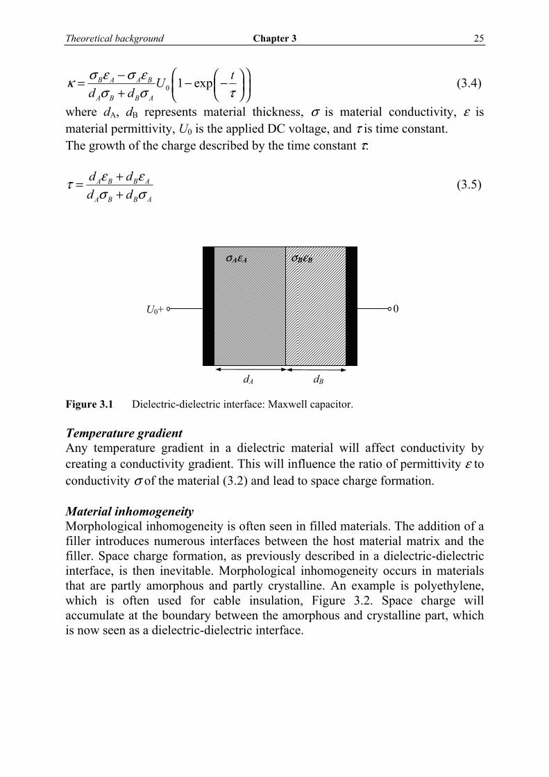
where dA, dB represents material thickness, σ is material conductivity, ε is material permittivity, U0 is the applied DC voltage, and τ is time constant. The growth of the charge described by the time constant τ:
A B B A
A B B A
d dd d
ε ετσ σ
+=+
(3.5)
Figure 3.1 Dielectric-dielectric interface: Maxwell capacitor. Temperature gradient Any temperature gradient in a dielectric material will affect conductivity by creating a conductivity gradient. This will influence the ratio of permittivity ε to conductivity σ of the material (3.2) and lead to space charge formation. Material inhomogeneity Morphological inhomogeneity is often seen in filled materials. The addition of a filler introduces numerous interfaces between the host material matrix and the filler. Space charge formation, as previously described in a dielectric-dielectric interface, is then inevitable. Morphological inhomogeneity occurs in materials that are partly amorphous and partly crystalline. An example is polyethylene, which is often used for cable insulation, Figure 3.2. Space charge will accumulate at the boundary between the amorphous and crystalline part, which is now seen as a dielectric-dielectric interface.
dA dB
U0+ 0
σAεA σBεB

26 Chapter 3 Theoretical background
Figure 3.2 Structure of a polymer with crystalline and amorphous parts. As already mentioned, several physical mechanisms are involved in space charge formation: Injection/extraction process The injection/extraction process of charge carriers at an electrode-dielectric interface is possible across or through the metal-dielectric potential barrier, which charge carriers at the electrode have to overcome to enter the dielectric material. The first type of injection is described by the Schottky process [24]. Application of an electric field leads to a reduction of a potential barrier making charge injection possible across the potential barrier. The second type of injection through the potential barrier is described by the Fowler-Nordheim process [24] in which, at fields above approximately 100 kV/mm, the potential barrier becomes very narrow making charge carrier tunnelling possible. Injected charge carriers may also recombine if the opposite charge is present in their proximity. Trapping Trapping sites, or more simply traps, are potential wells where the charge carriers can be captured. Traps are always present in an insulating material due to the fact that insulating materials are never perfectly homogeneous: crystalline and amorphous regions may be found in a piece of material. At the atomic level, there will be significant changes in interatomic spacing due to structural disorders in amorphous regions, and this will cause spatial changes in the band gap [24]. Also, incompletely bound atoms in crystal defects give rise to so-called dangling bonds [41]. The dangling bonds can be satisfied by either the removal or donation of an electron (or both) and thus behave as states within the band gap. These localised energy states in the band gap are called trapping sites: donor trapping sites (hole traps) are located immediately above the top of the valence band, acceptor trapping sites (electron traps) are located immediately below the bottom of the conduction band. Electrons or holes crossing over from the valence to the conduction band may enter the trapping sites and may have to
crystalline amorphous

Theoretical background Chapter 3 27
acquire considerable energy before they can leave. So-called self-traps are also possible: the field from an electron or hole can re-orientate the local structure thereby creating a potential well from which escape may be very difficult. Traps are usually classified according to their location, in the vicinity of physical or chemical defects. Physical defects are conformational; they can be found close to a material surface and in the amorphous parts of materials at the ends of molecular chains. They are responsible for shallow physical trapping sites. Chemical defects consist of additives (for instance, antioxidants), cross-linking by-products, and other impurities. They are responsible for deeper chemical traps. Charge carriers will be trapped at a rate dependent upon their initial kinetic energy. Transportation There will always be a certain amount of injected charge carriers that will be transported through the dielectric and finally extracted. Some of them move free, others are trapped on their way through the dielectric and then, after some time, released. Therefore, the transportation of charge carriers depends also on the density and depth of the trapping sites. This is often denoted as trap limited conduction [50], Figure 3.3. Figure 3.3 Charge carrier transport through dielectric material is defined by the density
and depth of trapping sites. The time a charge carrier spends in a trap is much greater than the time spent travelling between the traps. For example: an electron travels with a velocity of approximately 105 m/s between the traps and spends more than an hour in traps of depth 1 eV.
The time that a charge carrier spends in a trap is much greater than the time spent travelling between the traps. For example: an electron travels with a velocity of approximately 105 m/s between the traps and spends more than an hour in traps of depth 1 eV.
Potential energy
[eV]
2 eV ~ billions of years
0.5 eV ~ 1 μs 1 eV~ 1 hour
~ 105 m/s
0
x

28 Chapter 3 Theoretical background
Charge generation Charge carriers which form space charge are injected from the electrodes or are generated in the material bulk. The internal charge carriers can be electrons or holes that have gained sufficient energy to escape from the valence band into the conduction band. The corresponding excitation energy can be of thermal, electrical, or of some other radiative nature. The charge carriers are sometimes ions, which can be present in the material for various reasons: they can be formed due to the dissociation [51] of additives and impurities that are often found in insulating materials, or they can be a by-product of aging [52].
3.3 Conduction current
Conduction current is the part of a polarisation current that is measured when a DC voltage is applied across the insulating material. The polarisation current has a decreasing character, and when all polarisation processes are finished, it approaches its steady-state value: conduction current. An example of a plot of polarisation current versus polarisation time is given in Figure 3.4.
Figure 3.4 Polarisation current in pre-stressed PCTiO2. Applied electric field
17.1 kV/mm. Polarisation current is given by expression (3.6), [51], [53], Appendix E:
( ) ( ) ( )0 00
PI t U C t f tσ δε
⎡ ⎤= + +⎢ ⎥
⎣ ⎦ (3.6)
where: C0 is geometrical capacity, U0 is applied DC voltage, δ(t) is a Dirac pulse, f(t) is the dielectric response function related to polarisation processes, ε0
is the vacuum permittivity, and σ is the material conductivity. When the conduction current is plotted against different applied electric fields, the E vs. I characteristic is obtained, as given in Figure 3.5.
PCTiO2 applied field E = 17.1 kV/mm
0.001
0.01
0.1
1
10
10 100 1000 10000 100000 time [sec]
curr
ent [
pA]

Theoretical background Chapter 3 29
Figure 3.5 E vs. I characteristic: change of degree of inclination from 1:1 (ohmic
behaviour) to 2:1, indicating the change of conducting mechanisms in the material.
Taking into consideration a parallel plane electrode configuration (which is used in the research described in this thesis), in the absence of space charge, the electric field in the material is uniform and a linear relationship exists between the conduction current through the material and the applied voltage. This linear relationship is described by Ohm’s law. The linear E vs. I characteristic plotted in a log-log plot is a straight line with a degree of inclination (slope) equal to one. The degree of inclination of the characteristic can also change, indicating a change of conduction mechanisms. For instance, in the presence of space charge, the internal electric field in the material is modified and the linear relationship does not hold anymore. Therefore, the threshold field at which the degree of the inclination of the E vs. I characteristic changes, coincides in many cases with the threshold field for space charge accumulation.
3.4 Dielectric polarisation and relaxation
The majority of dielectric materials used in electrical power engineering can be described as being isotropic and linear [53], [55]. For these materials, polarisation
→
P is proportional to the applied electric field →
E through the relationship (3.7): →
P = ε0 (εr –1)→
E (3.7) where ε0 is the vacuum permittivity and εr is the relative permittivity. The process opposing polarization is called relaxation and each dielectric structure has a characteristic relaxation frequency or frequency band. The permittivity, ε = ε0εr, in an alternating electric field is a complex quantity and a function of frequency, (3.8):
a.u. E [kV/mm]
Con
duct
ion
curr
ent [
A]
a.u
. ohmic behavior
non-ohmic behavior

30 Chapter 3 Theoretical background
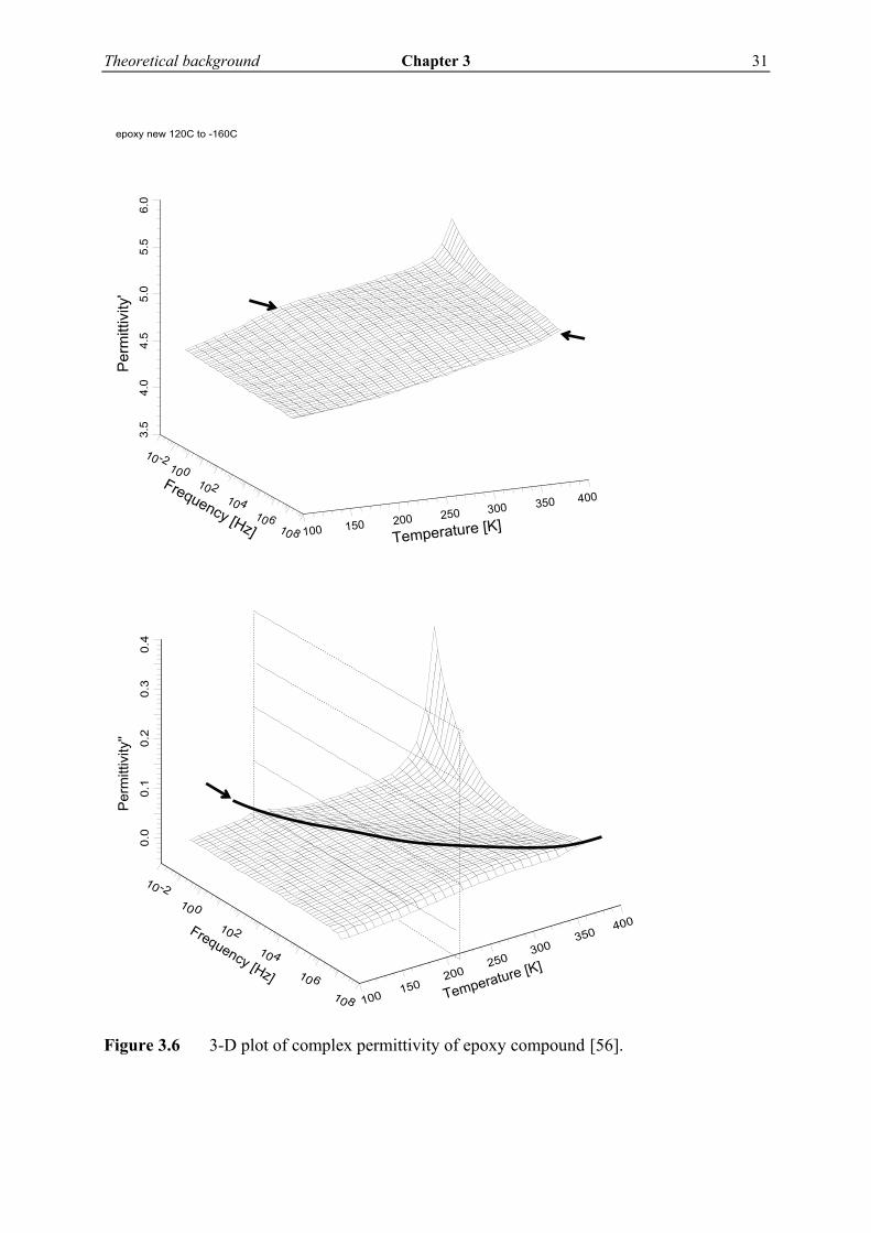
ε(ω) = ε΄(ω)- iε΄΄(ω) (3.8) ε΄(ω) is the real part of complex permittivity and represents a measure for the energy stored per period. ε΄΄(ω) is the imaginary part of complex permittivity and represents energy dissipated per period or dielectric absorption. The ratio between the real and the imaginary part of complex permittivity is termed tan δ, (3.9). tan δ is actually the phase lag between the alternating voltage V applied at a capacitor and current I through the capacitor1. tan δ= ε΄΄/ε΄ (3.9) tan δ is frequently used in practice for the testing of insulation materials and the measurements are usually performed at single frequency, 50 Hz. However, a lot more information about the structure and condition of insulating materials is available when complex permittivity is observed in a broad frequency range. Complex permittivity is not only a function of the frequency of an applied electric field, it is also temperature dependent. An example of 3 - D plots of real and imaginary parts of complex permittivity is given in Figure 3.6 [56]. The relationship between complex permittivity, frequency, and temperature [57] was first found by Debye, (3.10):
( ) ( )TiT, s
ωτεεεωε
+−=− ∞
∞ 1 (3.10)
where ε∞ is the dielectric constant at ω → ∞, εs is the dielectric constant at ω → 0, and τ(T) is the relaxation time. The real and the imaginary parts of complex permittivity can be written as (3.11) - (3.12):
( ) ( )TT,' s
221 τωεεεωε
+−=− ∞
∞ (3.11)
( ) ( ) ( )( )T
TT,'' s 221 τωωτεεωε
+−= ∞ (3.12)
1 When an alternating voltage is applied to a capacitor the current through the capacitor will consist of two parts: Real (resistive) part which is in phase with the applied voltage, IR = ωC0ε΄΄V Imaginary (capacitive) part, out of phase, IC = iωC0ε΄V Phase lag between applied alternating voltage V and current I, termed δ, is given with tanδ = ε΄΄/ε΄
Theoretical background Chapter 3 31
10 -210 0
10 210 4
10 610 8
Frequency [Hz]
3.5
4.0
4.5
5.0
5.5
6.0
Per
mitt
ivity
'
100 150 200 250 300 350 400
Temperature [K]
epoxy new 120C to -160C
10 -210 0
10 2
10 4
10 610 8
Frequency [Hz]
0.0
0.1
0.2
0.3
0.4
Per
mitt
ivity
''
100 150200
250300
350 400
Temperature [K]
Figure 3.6 3-D plot of complex permittivity of epoxy compound [56].
32 Chapter 3 Theoretical background
The relationship described by (3.10) assumes one specific relaxation time τ(T). Therefore (3.10) is valid for gasses and liquids with a low molecular content where assumption of one polar group is generally acceptable. For a polymer, some modifications are needed. A polymer often contains different polar groups, and more than one interaction with its neighbours. As a consequence, there is more than one relaxation time, and a certain fluctuation in relaxation time. In other words, a polar group is characterised by a number of relaxation times that are grouped around a certain mean relaxation time. Cole-Cole introduced a modification of (3.10) as given by (3.13):
( )( )
,1
sTi T β
ε εε ω εωτ
∞∞
−− =+ ⎡ ⎤⎣ ⎦
(3.13)
The factor β makes possible a symmetrical spread of relaxation times along the frequency axis. Another modification of the Debye expression, which is more general than (3.13), was made by Havriliak and Negami:
( )( )
,1
sTi T
αβ
ε εε ω εωτ
∞∞
−− =+ ⎡ ⎤⎣ ⎦
(3.14)
Complex permittivity exhibits several types of relaxation, each of them characterised by their own relaxation parameters. The most pronounced is α-relaxation. α-relaxation has a high and narrow peak in comparison with other relaxations; at higher temperatures the maximum extent of the relaxation shifts to higher frequencies. In polymers, this relaxation is associated with the glass transition temperature, Tg, and it is caused by the co-operative motion of a number of (polar) segments of the main molecular chain. So-called β-relaxation is characterised by a broad relaxation peak, which can have a width of several decades. The position of the maximum extent of β-relaxation also shifts to higher frequencies if the temperature is increased. This relaxation arises from localised rotational fluctuations of side groups, or fluctuations of localised parts of the main molecule chain. α-relaxation shows non-Arrhenius temperature dependence, while β-relaxation does. The α- and β-relaxation peaks have no fixed distance: this is strongly influenced by molecular structure and by different behaviour relating to temperature dependence. Therefore, it can happen that these two types of relaxation merge,

Theoretical background Chapter 3 33
making a distinction between them quite difficult. An example is given in Figure 3.7. Figure 3.7 An example of ε΄΄ and contributions of α- and β-relaxations.
α-relaxation
β-relaxation
ε΄΄
ε΄΄
log f [Hz]a.u.
a.u.

34 Chapter 3 Theoretical background

The effect of long term DC stress on space charge dynamics Chapter 4 35
TThhee eeffffeecctt ooff lloonngg--tteerrmm DDCC ssttrreessss oonn ssppaaccee cchhaarrggee ddyynnaammiiccss
44 4.1 Introduction
Space charge measurements provide us with a means to detect magnitude, polarity and location of charge trapped in a dielectric. From the measured space charge profile, the distribution of the electric field is derived and as such, space charge measurements are a valuable tool for dielectric evaluation. Furthermore, different dielectrics can be compared regarding their tendency to accumulate charge: it appears that for many dielectrics a threshold field can be defined below which no or hardly any space charge accumulates. This chapter presents results of space charge measurements performed in order to establish the space charge dynamics of PC and PC-TiO2, and to analyse the effect of long-term exposure to a high electric DC field (100 kV/mm DC for 1500 hours) on the space charge behaviour of materials. Space charge measurements were performed using the PEA method on flat PC and PC-TiO2 specimens as explained in Chapter 2: Experimental. Generally speaking, for the purposes of PEA measurements, an electric pulse is applied to the specimen, resulting in a perturbation force at the location of space charge.
36 Chapter 4 The effect of long term DC stress on space charge dynamics
As a consequence, an acoustic wave is generated which is detected by a piezoelectric sensor. The voltage signal provided by the piezoelectric sensor contains information about the density and location of space charge. Based on the space charge measurements, a number of space charge related quantities are calculated and derived, as listed below:
Space charge density and polarity, and the position of accumulated space charge.
Electrical field strength in the material. Space charge accumulation (and depletion) characteristic times. Characteristics of space charge density as a function of a polarising
electric field (ρ vs. E characteristics). Electrical threshold for space charge accumulation, Eth,sc.
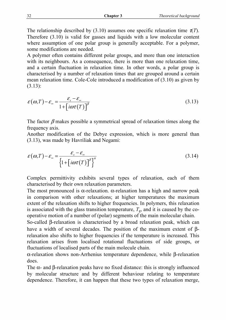
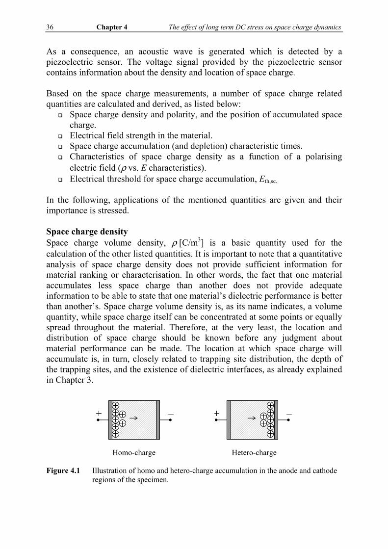
In the following, applications of the mentioned quantities are given and their importance is stressed. Space charge density Space charge volume density, ρ [C/m3] is a basic quantity used for the calculation of the other listed quantities. It is important to note that a quantitative analysis of space charge density does not provide sufficient information for material ranking or characterisation. In other words, the fact that one material accumulates less space charge than another does not provide adequate information to be able to state that one material’s dielectric performance is better than another’s. Space charge volume density is, as its name indicates, a volume quantity, while space charge itself can be concentrated at some points or equally spread throughout the material. Therefore, at the very least, the location and distribution of space charge should be known before any judgment about material performance can be made. The location at which space charge will accumulate is, in turn, closely related to trapping site distribution, the depth of the trapping sites, and the existence of dielectric interfaces, as already explained in Chapter 3. Homo-charge Hetero-charge Figure 4.1 Illustration of homo and hetero-charge accumulation in the anode and cathode
regions of the specimen.
The effect of long term DC stress on space charge dynamics Chapter 4 37
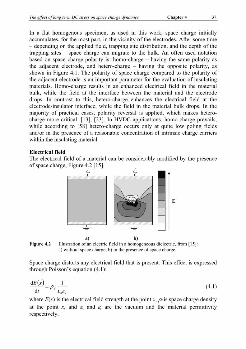
In a flat homogenous specimen, as used in this work, space charge initially accumulates, for the most part, in the vicinity of the electrodes. After some time – depending on the applied field, trapping site distribution, and the depth of the trapping sites – space charge can migrate to the bulk. An often used notation based on space charge polarity is: homo-charge – having the same polarity as the adjacent electrode, and hetero-charge – having the opposite polarity, as shown in Figure 4.1. The polarity of space charge compared to the polarity of the adjacent electrode is an important parameter for the evaluation of insulating materials. Homo-charge results in an enhanced electrical field in the material bulk, while the field at the interface between the material and the electrode drops. In contrast to this, hetero-charge enhances the electrical field at the electrode-insulator interface, while the field in the material bulk drops. In the majority of practical cases, polarity reversal is applied, which makes hetero-charge more critical. [13], [23]. In HVDC applications, homo-charge prevails, while according to [58] hetero-charge occurs only at quite low poling fields and/or in the presence of a reasonable concentration of intrinsic charge carriers within the insulating material. Electrical field The electrical field of a material can be considerably modified by the presence of space charge, Figure 4.2 [15]. a) b) Figure 4.2 Illustration of an electric field in a homogeneous dielectric, from [15]:
a) without space charge, b) in the presence of space charge. Space charge distorts any electrical field that is present. This effect is expressed through Poisson’s equation (4.1):
( ) txE
rf εε
ρ0
1d
d = (4.1)
where E(x) is the electrical field strength at the point x, ρf is space charge density at the point x, and ε0 and εr are the vacuum and the material permittivity respectively.
E

38 Chapter 4 The effect of long term DC stress on space charge dynamics
The presence of space charge in a dielectric implies that the dielectric experiences electrical fields above design values in some regions. This additional electrical stress is very hard to take into consideration in the original insulation design, due to the fact that space charge accumulation is influenced by a variety of factors that change during the lifetime of the insulation. Generally speaking, polymeric insulating materials do not indefinitely retain the nature that they possessed on first being manufactured. Over a period of time, both their chemical composition and physical morphology may change, even when not exposed to electrical stress. An enhancement factor f can be calculated as (4.2):
max 100%DC
DC
E EfE
−= ⋅ (4.2)
where EDC denotes the applied electric field, and Emax is the maximum of the actual field strength in the test-specimen. Space charge accumulation and depletion characteristic times Both charge accumulation and depletion processes are often described with more than one exponential function and corresponding time constants, as schematically depicted in Figure 4.3. The existence of several time constants is brought about by the processes that take place in the material during the accumulation period [23-24]. These are: injection/extraction, transportation, and recombination of the charge carriers. Figure 4.3 Illustration of space charge accumulation and depletion processes in time. In analytical form, the processes are described by a superposition of exponential functions according to the following expression (4.3):
( ) ( )∑ −==
−n
i
t
iiitotal etxt
1)1( τρρ (4.3)
accumulation time [s]
spac
e ch
arge
den
sity
[C
/m3 ]
slow build up
fast growth
depletion time [s]
spac
e ch
arge
den
sity
[C
/m3 ]
slow decay
rapid decay

The effect of long term DC stress on space charge dynamics Chapter 4 39
where ρtotal(t) is the total amount of accumulated charge, ρi(t) is a part of the total charge accumulated during the process described by an exponential function with the corresponding time constant τi, and x is a weight factor. According to [24], since charging phenomena are frequently affected by polarity, time constants can demonstrate polarity dependence. From a practical point of view, it is also interesting to know when the majority of the charging and discharging processes are completed: a limitation can be set at approximately 90 %, which fits quite well in the regions described as fast growth or rapid decay in Figure 4.4. In this way, the accumulation and depletion processes, or 90 % of the processes, are characterised with one exponential function and thus one time constant. Weather the 90 % accumulation and depletion time constants will be the same or not depends on space charge distribution within the material specimen. In cases where there is absolute space charge symmetry in a homogeneous material specimen, space charge will be driven out of the specimen at the same rate as it was accumulated. In contrast to this, in the most probable unsymmetrical charge distribution, a part of the accumulated charge will be driven out and a part will be forced into the bulk of the specimen. Consequently, depletion will take more time than accumulation. This is illustrated in Figure 4.4 a)-b) from [24]. Figure 4.4 Direction of charge motion in a short-circuited specimen from [24].
a) Symmetrical charge distribution, a zero field plane in the centre of the specimen.
b) Unsymmetrical charge distribution, zero-field planes outside the centre of the specimen
The practical significance of charge depletion time is that it gives the characteristic discharge time needed to release the internal DC stress of the material. It is also related to processes on a microscopic scale: the depth and distribution of trapping sites can be influenced by long-term exposure to a high
Sample
Hetrocharge Homocharge Zero field plane
Direction of charge motion
Sample
Homocharge Homocharge Zero field planes
Direction of charge motion
40 Chapter 4 The effect of long term DC stress on space charge dynamics
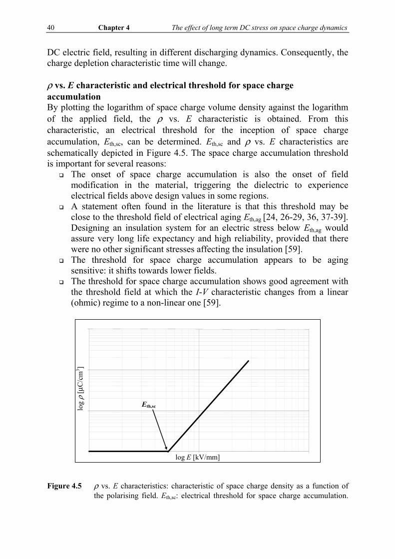
DC electric field, resulting in different discharging dynamics. Consequently, the charge depletion characteristic time will change. ρ vs. E characteristic and electrical threshold for space charge accumulation By plotting the logarithm of space charge volume density against the logarithm of the applied field, the ρ vs. E characteristic is obtained. From this characteristic, an electrical threshold for the inception of space charge accumulation, Eth,sc, can be determined. Eth,sc and ρ vs. E characteristics are schematically depicted in Figure 4.5. The space charge accumulation threshold is important for several reasons:
The onset of space charge accumulation is also the onset of field modification in the material, triggering the dielectric to experience electrical fields above design values in some regions.
A statement often found in the literature is that this threshold may be close to the threshold field of electrical aging Eth,ag [24, 26-29, 36, 37-39]. Designing an insulation system for an electric stress below Eth,ag would assure very long life expectancy and high reliability, provided that there were no other significant stresses affecting the insulation [59].
The threshold for space charge accumulation appears to be aging sensitive: it shifts towards lower fields.
The threshold for space charge accumulation shows good agreement with the threshold field at which the I-V characteristic changes from a linear (ohmic) regime to a non-linear one [59].
Figure 4.5 ρ vs. E characteristics: characteristic of space charge density as a function of
the polarising field. Eth,sc: electrical threshold for space charge accumulation.
log E [kV/mm]
log
ρ [μ
C/cm
3 ]
Eth,sc

The effect of long term DC stress on space charge dynamics Chapter 4 41
Eth,sc denotes the onset of space charge accumulation, which is supposed [59] to be close to the threshold field of electrical aging.
4.2 Charge dynamics of virgin and pre-stressed PC: results of the measurements
In this section, the results of space charge measurements on virgin and pre-stressed PC specimens are presented. In so doing, space charge quantities are considered, as listed in the introduction to this chapter.
4.2.1 Density, polarity and position of accumulated space charge
The density1 of space charge accumulated during 3 hours of poling in the PEA measuring set-up ranges from2 0.05 μC/cm3 to 2 μC/cm3. Space charge density is slightly lower for pre-stressed PC. For both new and pre-stressed specimens, homo-charge was detected in the vicinity of the electrodes. Figures 4.6-4.7. show typical space charge profiles plotted against a specimen thickness, measured 10 minutes after switching off the applied DC voltage. Figure 4.6 Homo-charge in virgin PC specimens. Applied electric field was 45.7 kV/mm
for 3 hours. The measurements were carried out 10 minutes after switching off the applied field.
1 Mean density over total specimen volume. 2 Detection limit of the PEA measuring set-up is between 0.03 μC/cm3 and 0.05 μC/cm3. Uncertainty of the measurement results is assumed to be about 15 %, see Chapter 2: Experimental.
new PC
-6
-4
-2
0
2
4
6
0.1 0.2 0.3 0.4
specimen thickness [mm]
ρ [μ
C/cm
3 ]
mirror charge HV electrode
mirror charge ground electrode
homo-charge
ground electrode HV electrode
42 Chapter 4 The effect of long term DC stress on space charge dynamics
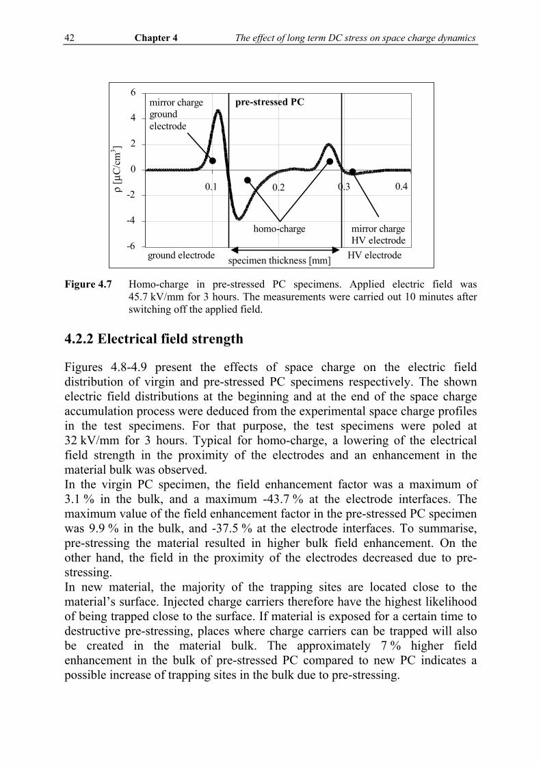
Figure 4.7 Homo-charge in pre-stressed PC specimens. Applied electric field was
45.7 kV/mm for 3 hours. The measurements were carried out 10 minutes after switching off the applied field.
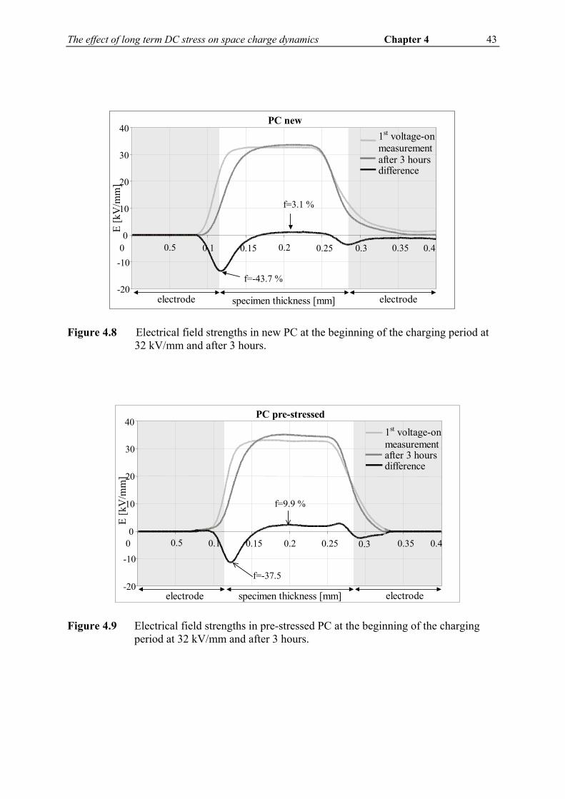
4.2.2 Electrical field strength
Figures 4.8-4.9 present the effects of space charge on the electric field distribution of virgin and pre-stressed PC specimens respectively. The shown electric field distributions at the beginning and at the end of the space charge accumulation process were deduced from the experimental space charge profiles in the test specimens. For that purpose, the test specimens were poled at 32 kV/mm for 3 hours. Typical for homo-charge, a lowering of the electrical field strength in the proximity of the electrodes and an enhancement in the material bulk was observed. In the virgin PC specimen, the field enhancement factor was a maximum of 3.1 % in the bulk, and a maximum -43.7 % at the electrode interfaces. The maximum value of the field enhancement factor in the pre-stressed PC specimen was 9.9 % in the bulk, and -37.5 % at the electrode interfaces. To summarise, pre-stressing the material resulted in higher bulk field enhancement. On the other hand, the field in the proximity of the electrodes decreased due to pre-stressing. In new material, the majority of the trapping sites are located close to the material’s surface. Injected charge carriers therefore have the highest likelihood of being trapped close to the surface. If material is exposed for a certain time to destructive pre-stressing, places where charge carriers can be trapped will also be created in the material bulk. The approximately 7 % higher field enhancement in the bulk of pre-stressed PC compared to new PC indicates a possible increase of trapping sites in the bulk due to pre-stressing.
pre-stressed PC
-6
-4
-2
0
2
4
6
0.1 0.2 0.3 0.4
mirror charge HV electrode
mirror charge ground electrode
homo-charge
ρ [μ
C/c
m3 ]
specimen thickness [mm] ground electrode HV electrode
The effect of long term DC stress on space charge dynamics Chapter 4 43
Figure 4.8 Electrical field strengths in new PC at the beginning of the charging period at
32 kV/mm and after 3 hours.
Figure 4.9 Electrical field strengths in pre-stressed PC at the beginning of the charging
period at 32 kV/mm and after 3 hours.
PC pre-stressed
40
specimen thickness [mm]
E [k
V/m
m]
1st voltage-on measurement after 3 hoursdifference
electrode electrode -20
-10
0
10
20
30
0 0.5 0.1 0.15 0.2 0.25 0.3 0.35 0.4
f=9.9 %
f=-37.5
PC new E
[kV
/mm
]
1st voltage-on measurement
difference
-20
-10
0
10
20
30
40
0 0.5 0.1 0.15 0.2 0.25 0.3 0.35
f=3.1 %
f=-43.7 %
specimen thickness [mm] electrode electrode
0.4
after 3 hours
44 Chapter 4 The effect of long term DC stress on space charge dynamics
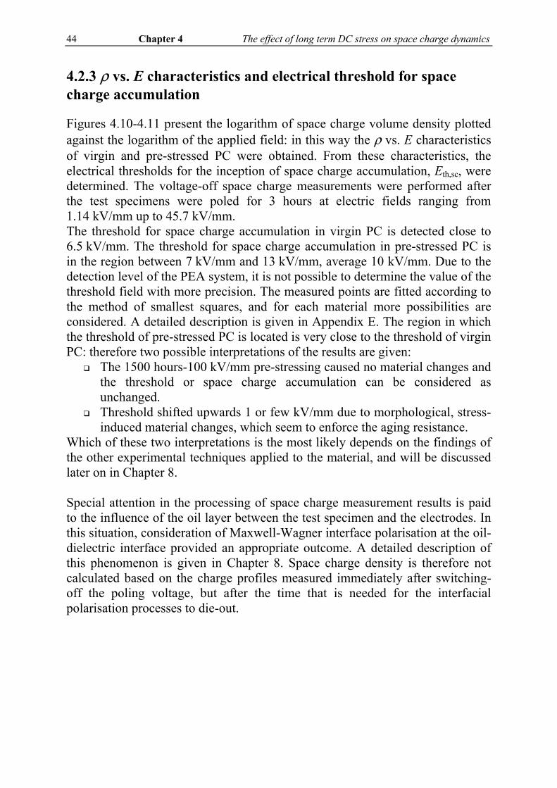
4.2.3 ρ vs. E characteristics and electrical threshold for space charge accumulation
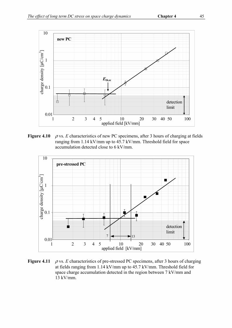
Figures 4.10-4.11 present the logarithm of space charge volume density plotted against the logarithm of the applied field: in this way the ρ vs. E characteristics of virgin and pre-stressed PC were obtained. From these characteristics, the electrical thresholds for the inception of space charge accumulation, Eth,sc, were determined. The voltage-off space charge measurements were performed after the test specimens were poled for 3 hours at electric fields ranging from 1.14 kV/mm up to 45.7 kV/mm. The threshold for space charge accumulation in virgin PC is detected close to 6.5 kV/mm. The threshold for space charge accumulation in pre-stressed PC is in the region between 7 kV/mm and 13 kV/mm, average 10 kV/mm. Due to the detection level of the PEA system, it is not possible to determine the value of the threshold field with more precision. The measured points are fitted according to the method of smallest squares, and for each material more possibilities are considered. A detailed description is given in Appendix E. The region in which the threshold of pre-stressed PC is located is very close to the threshold of virgin PC: therefore two possible interpretations of the results are given:
The 1500 hours-100 kV/mm pre-stressing caused no material changes and the threshold or space charge accumulation can be considered as unchanged.
Threshold shifted upwards 1 or few kV/mm due to morphological, stress-induced material changes, which seem to enforce the aging resistance.
Which of these two interpretations is the most likely depends on the findings of the other experimental techniques applied to the material, and will be discussed later on in Chapter 8. Special attention in the processing of space charge measurement results is paid to the influence of the oil layer between the test specimen and the electrodes. In this situation, consideration of Maxwell-Wagner interface polarisation at the oil-dielectric interface provided an appropriate outcome. A detailed description of this phenomenon is given in Chapter 8. Space charge density is therefore not calculated based on the charge profiles measured immediately after switching-off the poling voltage, but after the time that is needed for the interfacial polarisation processes to die-out.
The effect of long term DC stress on space charge dynamics Chapter 4 45
Figure 4.10 ρ vs. E characteristics of new PC specimens, after 3 hours of charging at fields
ranging from 1.14 kV/mm up to 45.7 kV/mm. Threshold field for space accumulation detected close to 6 kV/mm.
Figure 4.11 ρ vs. E characteristics of pre-stressed PC specimens, after 3 hours of charging
at fields ranging from 1.14 kV/mm up to 45.7 kV/mm. Threshold field for space charge accumulation detected in the region between 7 kV/mm and 13 kV/mm.
0.01
0.1
1
10
char
ge d
ensi
ty [μ
C/c
m3 ]
applied field [kV/mm]
new PC
1 10 100 2 3 4 5 20 30 40 50
Eth,sc
detection limit
pre-stressed PC
0.01
0.1
1
10
char
ge d
ensi
ty [ μ
C/c
m3 ]
applied field [kV/mm]1 10 100 2 3 4 5 20 30 40 50
detection limit
7 13
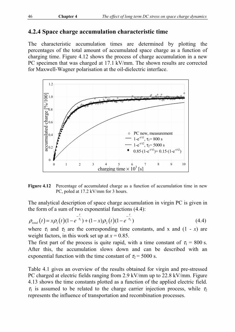
46 Chapter 4 The effect of long term DC stress on space charge dynamics
4.2.4 Space charge accumulation characteristic time
The characteristic accumulation times are determined by plotting the percentages of the total amount of accumulated space charge as a function of charging time. Figure 4.12 shows the process of charge accumulation in a new PC specimen that was charged at 17.1 kV/mm. The shown results are corrected for Maxwell-Wagner polarisation at the oil-dielectric interface.
Figure 4.12 Percentage of accumulated charge as a function of accumulation time in new
PC, poled at 17.2 kV/mm for 3 hours. The analytical description of space charge accumulation in virgin PC is given in the form of a sum of two exponential functions (4.4):
( ) ( ) ( )1 21 2(1 ) (1 ) (1 )
t t
total t x t e x t eτ τρ ρ ρ− −
= − + − − (4.4) where τ1 and τ2 are the corresponding time constants, and x and (1 - x) are weight factors, in this work set up at x = 0.85. The first part of the process is quite rapid, with a time constant of τ1 = 800 s. After this, the accumulation slows down and can be described with an exponential function with the time constant of τ2 = 5000 s. Table 4.1 gives an overview of the results obtained for virgin and pre-stressed PC charged at electric fields ranging from 2.9 kV/mm up to 22.8 kV/mm. Figure 4.13 shows the time constants plotted as a function of the applied electric field. τ1 is assumed to be related to the charge carrier injection process, while τ2 represents the influence of transportation and recombination processes.
0
0.2
0.4
0.6
0.8
1.0
1.2
0 1 2 3 4 5 6 7 8 9 10 charging time × 103 [s]
accu
mul
ated
cha
rge
[%/1
00]
PC new, measurement 1-e-t/τ1, τ1= 800 s 1-e-t/τ2, τ2= 5000 s0.85⋅(1-e-t/τ1)+ 0.15⋅(1-e-t/τ2)

The effect of long term DC stress on space charge dynamics Chapter 4 47
τ1 of virgin, as well as pre-stressed, PC is quite low, up to 5.7 kV, with a mean value of approximately 400 s. The mean value of τ1 increased to 1500 s at higher applied fields. No relation was found with the applied electric field. No influence of pre-stressing was observed. τ2 remained almost constant for virgin PC with a mean value of 4300 s. In the case of pre-stressed PC, the value of the time constant increased for applied fields higher than 5.7 kV/mm. As for τ1, no relation was found with the applied electric field. Table 4.1 Accumulation time constants in virgin and pre-stressed PC
Electric field [kV/mm]
Virgin PC τ1 [s] τ2 [s]
Pre-stressed PC τ1 [s] τ2 [s]
2.9 0.3 × 10³ 2.0 × 10³ 0.9 × 10³ 6.0 × 10³ 5.7 0.5 × 10³ 6.0 × 10³ 0.8 × 10³ 3.0 × 10³ 11.4 2.0 × 10³ 4.0 × 10³ 1.7 × 10³ 25 × 103 17.1 0.8 × 10³ 5.0 × 10³ 1.7 × 10³ 10 × 103 22.8 1.8 × 10³ 4.5 × 10³ 1.2 × 10³ 15 × 103 34.3 -- -- 1.7 × 10³ 40 × 103
Figure 4.13 Time constants τ1 and τ2 as a function of applied field in virgin and pre-
stressed PC. τ1 - Up to 5.7 kV: mean value of is approximately 400 s. At higher applied fields: the mean value 1500 s. τ2 - Virgin PC: τ2 remained almost constant with a mean value 4300 s. Pre-stressed PC: the value of the time constant increased above 5.7 kV/mm.
PC, τ1
0
1
2
3
4
0 5 10 15 20 25 30 35E [kV/mm]
τ 1 x
103 [s
]
PC new PC pre-stressed
PC, τ2
0 5 10 15 20 25 30 35E [kV/mm]
0
10
20
30
40
τ 2 x
103 [s
]
PC new PC pre-stressed

48 Chapter 4 The effect of long term DC stress on space charge dynamics
4.3 Charge dynamics of virgin and pre-stressed PC-TiO2: results of the measurements
In this section, the results of the space charge measurements on virgin and pre-stressed PC-TiO2 specimens are shown. Thereby, space charge quantities are considered, as listed in the introduction of this chapter.
4.3.1 Density, polarity and position of accumulated space charge
The density of space charge accumulated during 3 hours of charging in the PEA measuring set-up ranges from 0.05 μC/cm3 to 1 μC/cm3. Homo-charge was detected in both virgin and pre-stressed specimens at charging fields up to 34.3 kV/mm. At higher fields, hetero-charge also started to accumulate in pre-stressed PC-TiO2. Typical examples are given in Figures 4.14-4.16. Figure 4.14 Homo-charge detected in virgin PC-TiO2 specimens; measurements performed
10 minutes after switching off 45.7 kV/mm charging field.
new PCTiO2
-3
-2
-1
0
1
2
3
0.1 0.2 0.3 0.4
specimen thickness [mm]
ρ [μ
C/c
m3
mirror charge HV electrode
mirror charge ground electrode
homo-charge

The effect of long term DC stress on space charge dynamics Chapter 4 49
Figure 4.15 Homo and hetero-charge detected in a pre-stressed PC-TiO2 specimen;
measurement done 10 minutes after switching off 45.7 kV/mm charging field. Figure 4.16 Homo and hetero-charge detected in a pre-stressed PC-TiO2 specimen;
measurement done 100 minutes after switching off 45.7 kV/mm charging field.
4.3.2 Electrical field strength
The electrical field strengths in the test specimens at the beginning of charging at 32 kV/mm and after 3 hours are given in Figures 4.17-4.18. The field enhancement factor f, calculated according to (4.2), for the virgin PC-TiO2 specimen is f = 9.9 % in the bulk, and f = -44 % at the electrode interfaces.
pre-stressed PCTiO2
-3
-2
-1
0
1
2
3
0.1 0.2 0.3 0.4
specimen thickness [mm]
ρ [μ
C/c
m3 ]
mirror charge ground electrode
mirror charge HV electrode
homo-charge
hetero-charge
pre-stressed PCTiO2
-3
-2
-1
0
1
2
3
0.1 0.2 0.3 0.4
specimen thickness [mm]
ρ [μ
C/c
m3 ]
mirror charge HV electrode
mirror charge ground electrode
homo-charge
hetero-charge

50 Chapter 4 The effect of long term DC stress on space charge dynamics
In the pre-stressed PC-TiO2 specimen, the field enhancement factor is f = 2.9 % in the bulk, and f = -18.7 % at the electrode interfaces. In pre-stressed PC-TiO2, hetero-charge was also measured. The occurrence of hetero-charge, which compensates for the effect of homo-charge (lowering the electrical field in the proximity of the electrodes and increasing it in the bulk), explains the apparent improvement of pre-stressed PC-TiO2 in relation to internal field enhancement. Figure 4.17 Electrical field strengths in new PC-TiO2 at the beginning of poling at
32 kV/mm and after 3 hours. Figure 4.18 Electrical field strengths in pre-stressed PC-TiO2 at the beginning of poling at
32 kV/mm and after 3 hours.
new PCTiO2
E [k
V/m
m]
1st measurement voltage-on after 3 hours difference
-20
-10
0
10
20
30
40
0.5 0.1 0.15 0.2 0.25 0.3 0.35 0.4
f=9.9 %
f=-44 %
specimen thickness [mm] electrode electrode
pre-stressed PCTiO2
100kV/mm 1500 hours
E [k
V/m
m]
1st voltage-on measurement after 3 hours difference
-20
-10
0
10
20
30
40
0.5 0.1 0.15 0.2 0.25 0.3 0.35 0.4
f=2.9 %
f=-18.7 %
specimen thickness [mm] electrode electrode

The effect of long term DC stress on space charge dynamics Chapter 4 51
4.3.3 ρ vs. E characteristics and electrical threshold for space charge accumulation
By plotting the logarithm of space charge volume density against the logarithm of the applied field, the ρ vs. E characteristics of virgin and pre-stressed PC-TiO2 were obtained, as presented in Figures 4.19-4.20. From these characteristics, an electrical threshold for the inception of space charge accumulation was determined. The voltage-off space charge measurements were performed after the test specimens were poled for 3 hours at 1.14 kV/mm … 45.7 kV/mm. The threshold for space charge accumulation in virgin PC-TiO2 was found in the region between 3.3 kV/mm and 4.7 kV/mm, average 4.1 kV/mm. The threshold for space charge accumulation in pre-stressed PC-TiO2 is in the region between 2.8 kV/mm and 5.8 kV/mm, average 4.3 kV/mm. Space charge density is slightly lower in pre-stressed PC-TiO2. As in the case of PC, more possibilities are also considered here:
The 1500 hours-100 kV/mm pre-stressing caused no material changes and the threshold of space charge accumulation can be considered as unchanged.
Threshold shifted upwards 1 or few kV/mm due to morphological, stress-induced material changes, which seem to enforce the aging resistance.
The slight shift of the average electrical threshold field for space charge accumulation towards higher values in pre-stressed PC-TiO2 could be a consequence of hetero-charge occurrence, which compensates for homo-charge. Accumulation of hetero-charge is attributed to intrinsic carriers and will start at low poling fields. When the accumulation of homo-charge finally starts, the measured total charge density will still remain low or at zero for a certain range of poling fields because of the compensation of the hetero-charge. The threshold field for space charge accumulation will be found at the poling field in which the charge density of homo-charge becomes higher than the charge density of hetero-charge. No hetero-charge was measured in virgin PC-TiO2, therefore the hypothesis about hetero-charge compensation could provide a possible explanation for the shift of the threshold due to pre-stressing towards higher, instead of lower, electric fields.
Again, which of these interpretations is the most likely depends on the findings of the other experimental techniques applied to the material, and will be discussed later on in Chapter 8.
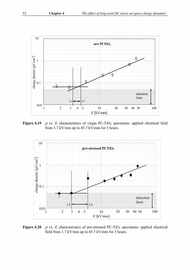
52 Chapter 4 The effect of long term DC stress on space charge dynamics
Figure 4.19 ρ vs. E characteristics of virgin PC-TiO2 specimens: applied electrical field
from 1.7 kV/mm up to 45.7 kV/mm for 3 hours.
Figure 4.20 ρ vs. E characteristics of pre-stressed PC-TiO2 specimens: applied electrical
field from 1.7 kV/mm up to 45.7 kV/mm for 3 hours.
new PCTiO2
0.01
0.1
1
10 ch
arge
den
sity
[μC
/cm
3 ]
E [kV/mm] 1 10 100 2 3 4 5 20 30 40 50
detection limit
3.3 4.7
E [kV/mm]
0.01
0.1
1
10
char
ge d
ensi
ty [μ
C/c
m3 ]
pre-stressed PCTiO2
1 10 1002 3 4 5 20 30 40 50
detection limit
5.82.8

The effect of long term DC stress on space charge dynamics Chapter 4 53
4.3.4 Space charge accumulation and depletion characteristic time
As in the case of PC, the accumulation process in PC-TiO2 is characterised by two time constants. Table 4.2 gives an overview of the time constants obtained for virgin and pre-stressed PC-TiO2. Figure 4.21 shows the time constants plotted as a function of applied electric field. τ1 of virgin PC-TiO2 exhibits an increasing character with increases in the applied field up to 11.4 kV/mm. For higher applied fields, τ1 decreases with increases in the applied field. τ1 of pre-stressed PC-TiO2 remains rather constant in the range of the applied field, with a mean value of approximately 1000 s. τ2 remains quite constant for virgin PC-TiO2, with a mean value of approximately 4000 s. In the case of pre-stressed PC-TiO2, the value of the time constant increases for applied fields higher than 5.7 kV/mm, but shows no relation with the applied field. Table 4.2 Accumulation time constants in virgin and pre-stressed PC-TiO2
Electric field [kV/mm]
Virgin PC-TiO2 τ1 [s] τ2 [s]
Pre-stressed PC-TiO2 τ1 [s] τ2 [s]
1.7 1.7 × 10³ 4.5 × 10³ 1.2 × 10³ 5.0 × 10³ 2.9 -- -- 0.8 × 10³ 5.5 × 10³ 5.7 3.0 × 10³ 5.0 × 10³ 1.6 × 10³ 9.0 × 10³ 11.4 3.5 × 10³ 4.0 × 10³ 1.1 × 10³ 6.0 × 10³ 17.1 1.2 × 10³ 3.5 × 10³ -- -- 22.8 0.6 × 10³ 4.0 × 10³ 1.5 × 10³ 8.0 × 10³ 34.3 -- -- 0.4 × 10³ 3.0 × 10³
Figure 4.21 Time constants τ1 and τ2 as a function of applied field in virgin and pre-
stressed PC-TiO2 τ1 - Virgin PC-TiO2: τ1 increases with increasing applied field up to 11.4 kV/mm. Pre-stressed PC-TiO2: τ1 remained almost constant with a mean value 1000 s. τ2 - Virgin PC-TiO2: τ2 remained almost constant with a mean value 4000 s. Pre-stressed PC-TiO2: the value of the time constant increased up to 5.7 kV/m
0
1
2
3
4
τ 1 x
103 [s
]
0 5 10 15 20 25 30 35E [kV/mm]
PCTiO2 new PCTiO2 pre-stressed
PCTiO2, τ1
2
4
6
8
10
0 5 10 15 20 25 30 35E [kV/mm]
PCTiO2 new PCTiO2 pre-stressed
PCTiO2, τ2
τ 1 x
103 [s
]
0

54 Chapter 4 The effect of long term DC stress on space charge dynamics
4.4 Influence of TiO2 filler
In this sub-section, the influence of TiO2 filler is discussed, based on the results of space charge measurements for virgin PC and PC-TiO2 specimens. The fact that the threshold for space charge accumulation shifts to lower fields in virgin filled PC is attributed to the addition of TiO2 filler, Figure 4.22. 16.7 % of TiO2 (weight) creates a considerable number of trapping sites at the filler-polymer interfaces, of which most are shallower than the original ones in PC [24, 59]. The large number of shallow traps can be easy filled, and/or left, causing an increase in charge carrier mobility. Consequently, the potential barrier for injection decreases, leading to a shift in the threshold for space charge accumulation towards lower fields.
Figure 4.22 Electrical threshold for space charge accumulation in virgin PC and
PC-TiO2. The threshold field is lowered due to the addition of TiO2. Analysing the field enhancement factors of virgin PC and virgin PC-TiO2 results in the conclusion that in both materials the electric field is lowered in the proximity of the electrodes due to homo-charge. The field enhancement factor in the proximity of the electrodes was approximately the same for virgin PC and PC-TiO2 (43.7 % and 44 %). Assuming that the addition of TiO2 filler introduces numerous trapping sites in the material, a statement can be made that in the proximity of the electrodes the surface defects prevail above the trapping sites due to the filler. The trapping sites introduced by TiO2 filler have considerable influence in the material bulk, thereby providing an explanation for the fact that the field enhancement in virgin PC-TiO2 is 9.9 %, and in virgin PC only 3.1 %.
PCTiO2
0.01
0.1
1
10
char
ge d
ensi
ty [μ
C/c
m3 ]
E [kV/mm] 1 10 100 2 3 4 5 20 30 40 50
detection limit
3.3 4.7
PC
PCTiO2: Eth,sc
PC: Eth,sc
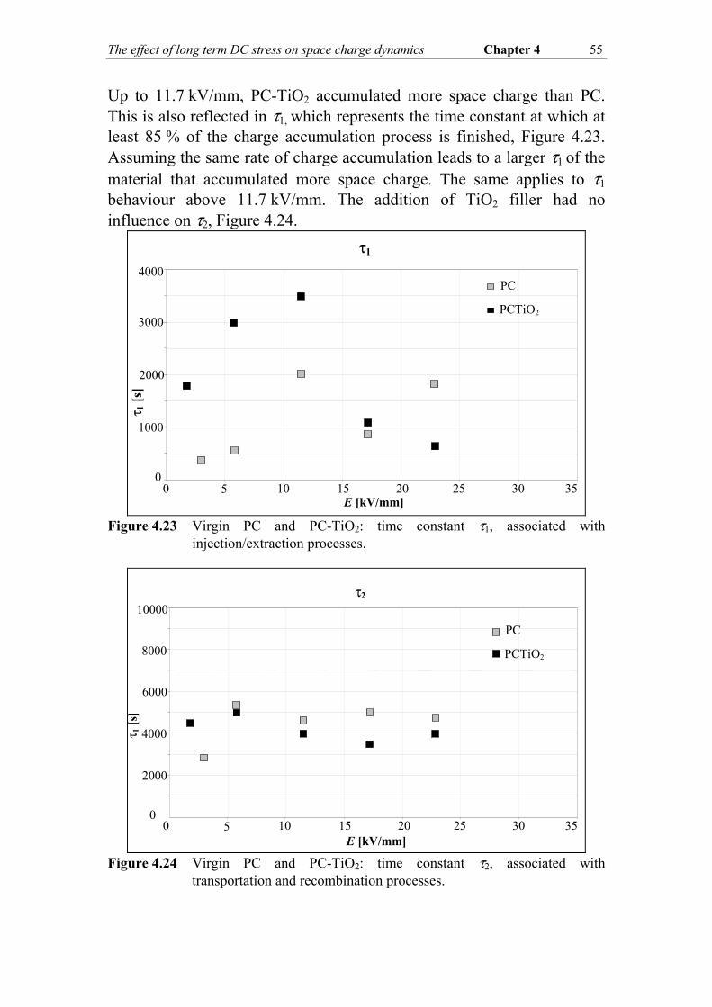
The effect of long term DC stress on space charge dynamics Chapter 4 55
Up to 11.7 kV/mm, PC-TiO2 accumulated more space charge than PC. This is also reflected in τ1, which represents the time constant at which at least 85 % of the charge accumulation process is finished, Figure 4.23. Assuming the same rate of charge accumulation leads to a larger τ1 of the material that accumulated more space charge. The same applies to τ1
behaviour above 11.7 kV/mm. The addition of TiO2 filler had no influence on τ2, Figure 4.24.
0
1000
2000
3000
4000
τ 1 [s
]
0 5 10 15 20 25 30 35 E [kV/mm]
PC
PCTiO2
τ1
Figure 4.23 Virgin PC and PC-TiO2: time constant τ1, associated with
injection/extraction processes.
2000
4000
6000
8000
10000
0 5 10 15 20 25 30 35 E [kV/mm]
PC
PCTiO2
τ2
τ 1 [s
]
0
Figure 4.24 Virgin PC and PC-TiO2: time constant τ2, associated with
transportation and recombination processes.

56 Chapter 4 The effect of long term DC stress on space charge dynamics
4.5 Summary and conclusions
Space charge measurements were performed by means of the PEA method on flat PC and PC-TiO2 specimens, with the objective of establishing the space charge dynamics of PC and PC-TiO2, and of analysing the effect of long-term exposure to a high electric DC field (100 kV/mm DC for 1500 hours) on the space charge behaviour of the materials. To introduce space charge, a DC electric field in the range 1.7 kV/mm … 45.7 kV/mm was applied across the test specimens for a period of 3 hours. The results of the measurements were corrected for Maxwell-Wagner polarisation at the oil-dielectric interface*. Based on the space charge measurements, a number of space charge related quantities were calculated and derived, as listed below:
Space charge density and polarity, and the position of accumulated space charge
Electrical field strength in the material Space charge accumulation (and depletion) characteristic times Characteristics of space charge density as a function of a polarising
electric field (ρ vs. E characteristics) Electrical threshold for space charge accumulation, Eth,sc
From the results of the space charge measurements on virgin and pre-stressed PC specimens, the following conclusions can be drawn: Homo-charge was detected in the proximity of the electrodes in both virgin and pre-stressed specimens. Homo-charge caused a lowering of the electrical field strength in the proximity of the electrodes, and field enhancement in the material bulk. Pre-stressing of the material resulted in a higher bulk field enhancement, whereas field lowering in the proximity of the electrodes decreased. A higher field enhancement in the bulk was explained by a possible increase of trapping sites due to pre-stressing. Both types of specimens showed threshold behaviour: the electrical threshold for space charge accumulation was found at approximately 6.5 kV/mm in virgin PC, and in the region between 7 kV/mm and 13 kV/mm in pre-stressed PC. Two possible interpretations of the results were given:
Threshold shifted upwards 1 or few kV/mm due to morphological, stress-induced material changes, which seem to enforce the aging resistance.
* Interposition of an oil droplet between the electrode and the test specimen during the space charge measurements is necessary in order to obtain a better acoustical coupling.

The effect of long term DC stress on space charge dynamics Chapter 4 57
The 1500 hours-100 kV/mm pre-stressing caused no material changes, and the threshold for space charge accumulation can be considered as unchanged.
The charging process was described with a sum of two exponential functions, whereby the longest one accounted for 85 % of the total accumulated charge. The corresponding time constants were related to charge injection (τ1), and to charge transportation and recombination (τ2). τ1 measured for PC appeared not to be influenced by pre-stressing. No relation was found with the applied electric field. τ2 seemed to be slightly influenced by pre-stressing: τ2 of virgin PC had a quite constant value, while τ2 of the pre-stressed specimens varied across a broad range. As for τ1, no relation was found with the applied electric field. From the results of the space charge measurements on virgin and pre-stressed PC-TiO2 specimens, the following conclusions can be drawn: Homo-charge was detected in the proximity of the electrodes in both virgin and pre-stressed specimens. In addition, hetero-charge was detected in the proximity of the HV electrodes of pre-stressed PC-TiO2. The field enhancement factor f for the new PC-TiO2 specimen was f = 9.9 % in the bulk, and f = -44 % at the electrode interfaces. In the pre-stressed PC-TiO2 specimen, the field enhancement factor was f = 2.9 % in the bulk, and f = -18.7 % at the electrode interfaces. The apparent improvement of pre-stressed PC-TiO2 in relation to the internal field enhancement was explained by the occurrence of hetero-charge, which compensated for the effect of homo-charge. The threshold for space charge accumulation in virgin PC-TiO2 was found in the region between 3.3 kV/mm and 4.7 kV/mm. The threshold for space charge accumulation in pre-stressed PC-TiO2 is in the region between 2.8 kV/mm and 5.8 kV/mm. Space charge density is slightly lower in pre-stressed PC-TiO2.Three possible explanations were given for this:
The shift of the electrical threshold field for space charge accumulation towards higher values in pre-stressed PC-TiO2 could be a consequence of hetero-charge occurrence compensating for homo-charge.
Threshold shifted upwards 1 or few kV/mm due to morphological, stress-induced material changes, which seem to enforce the aging resistance.
The 1500 hours-100 kV/mm pre-stressing caused no material changes and the threshold of space charge accumulation can be considered as unchanged.

58 Chapter 4 The effect of long term DC stress on space charge dynamics
The charging process was described with a sum of two exponential functions, whereby the longest one accounted for 85 % of the total accumulated charge. The corresponding time constants were related to the processes of charge injection/extraction, charge transportation, and charge recombination. τ1 of new PC-TiO2 exhibited an increasing character with increases in the applied field up to 11.4 kV/mm. For higher applied fields, τ1 decreased with increases in the applied field. τ1 of pre-stressed PC-TiO2 remained rather constant in the range of the applied field, showing no dependence on the applied field. τ2 remained constant for virgin PC-TiO2, with a mean value of approximately 4000 s. In the case of pre-stressed PC-TiO2, the value of the time constant increased for applied fields higher than 5.7 kV/mm, but showed no relation to the applied field. To summarise, both time constants appeared to be influenced by pre-stressing in a way that cannot be described analytically, but rather in terms of less fluctuation of τ1 and more fluctuation of τ2 around a mean value. The addition of TiO2 filler caused a lowering of the threshold field for space charge accumulation, which was not unexpected considering the fact that the filler introduced numerous interfaces in which space charge could accumulate. For the same reason, the field enhancement factor f was higher in the bulk of filled PC. In the proximity of the electrodes, surface defects prevailed over trapping sites due to the filler causing no changes in the field enhancement factor.

The effect of long term DC stress on space charge dynamics Chapter 4 59

60 Chapter 4 The effect of long term DC stress on space charge dynamics
Results of the polarization current measurements Chapter 5 61
RReessuullttss ooff tthhee ppoollaarriizzaattiioonn ccuurrrreenntt mmeeaassuurreemmeennttss 55
5.1 Introduction
This chapter presents the results of the polarization current measurements and conduction current analysis performed on the virgin and pre-stressed materials (100 kV/mm, 1500 hours) used in this thesis. The values of the conduction current, Icon, which are the steady-state values of the polarization current, are investigated as a function of the applied electric field. From the Icon vs. E characteristic, an electrical threshold field can be obtained at which any change of conduction mechanism from linear to non-linear takes place. Theoretical considerations show that this threshold level is quite close –if not identical- to the threshold for space charge accumulation. The presence of space charge excludes any ohmic conduction process and hence the two thresholds should more or less coincide. To verify the existence of such a threshold, polarization current measurements were performed allowing enough time for the polarization currents to disappear and the conduction current to show up.

62 Chapter 5 Results of the polarization current measurements
The electrical threshold field is associated with the onset of electrical aging [60, 36]. Therefore, it can be considered as an important parameter for insulation design and material characterization.
5.2 Polarization and conduction currents in PC: results of the measurements
The results of the polarization current measurements are presented in the form of graphs in which the polarization currents obtained for different polarizing fields are plotted as a function of time. For this purpose, polarizing fields in the range 2.9 kV/mm … 34.3 kV/mm were applied for 8 hours. Figures 5.1 and 5.2 show the results for virgin and pre-stressed PC specimens respectively. Two specimens were used for each experiment. When the current drops below the pA-level, the fluctuations in the measured values of the polarization current are quite large. Therefore, a moving average filter (window 2000 s) was used to minimize these fluctuations. Figures 5.3 and 5.4 show graphs of the steady-state values of the polarization current versus the applied electric field of virgin and pre-stressed PC specimens. In some cases, the (quasi) steady-state value of the polarization current - the conduction current - was not reached even after 8 hours of polarization time. The conduction currents were approximated using the following approach: the polarization currents can be fairly well described by the additive expression1 given in (5.1):
caa)( 21 n
2n
1 ++= −− tttI (5.1) where a1, a2, n1, n2, and c are constants, and t is the time. When t approaches infinity, only the constant c will remain. The constant c is actually the steady-state value of the polarization current, and therefore represents the conduction current, Icon. The values of the conduction current used for the E vs. Icon graph in Figures 5.3-5.4 were obtained by fitting formula (5.1) to the measurement results. The actual fits are shown in Appendix F. The values of Icon (E) obtained from different specimens deviate by approximately 10% to 12% as shown in the figures by means of error bars. The slope of the E vs. Icon log-log plot of virgin PC changes from 1 (ohmic behavior) to 2 close to 5 kV/mm, indicating a transition between different conduction mechanisms at that point. The slope of the E vs. Icon characteristic of pre-stressed PC shows no change: it remains approximately 2 in the entire range of the applied electric field. However, a slope larger than 1 represents a non-
1 The purpose of the used expression is to give the best fit: the physical meaning, if any, is not considered.
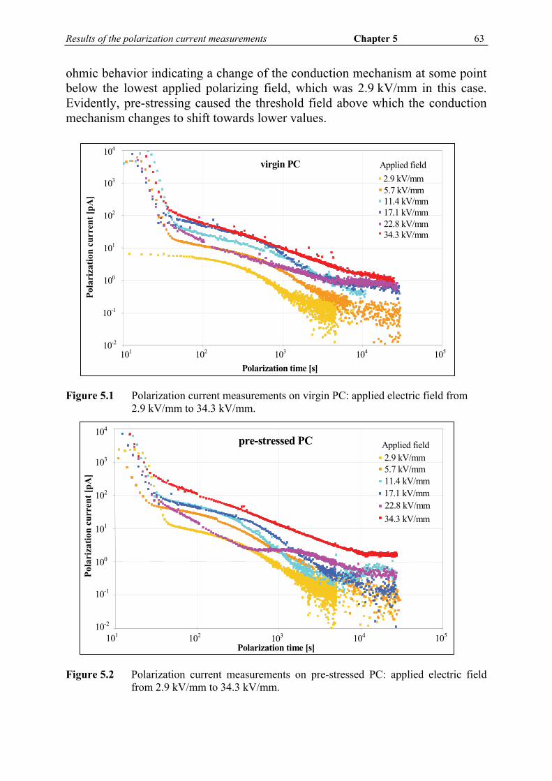
Results of the polarization current measurements Chapter 5 63
ohmic behavior indicating a change of the conduction mechanism at some point below the lowest applied polarizing field, which was 2.9 kV/mm in this case. Evidently, pre-stressing caused the threshold field above which the conduction mechanism changes to shift towards lower values.
Figure 5.1 Polarization current measurements on virgin PC: applied electric field from
2.9 kV/mm to 34.3 kV/mm.
Figure 5.2 Polarization current measurements on pre-stressed PC: applied electric field
from 2.9 kV/mm to 34.3 kV/mm.
virgin PC
10-2
10-1
100
101
102
103
104
Pola
riza
tion
curr
ent [
pA]
2.9 kV/mm 5.7 kV/mm 11.4 kV/mm 17.1 kV/mm 22.8 kV/mm 34.3 kV/mm
Applied field
101 102 Polarization time [s]
103 104 105
pre-stressed PC
101 102 103 104 105 Polarization time [s]
10-2
10-1
100
101
102
103
104
Pola
riza
tion
curr
ent [
pA]
2.9 kV/mm 5.7 kV/mm 11.4 kV/mm 17.1 kV/mm 22.8 kV/mm 34.3 kV/mm
Applied field

64 Chapter 5 Results of the polarization current measurements
Figure 5.3 Virgin PC: conduction current versus applied electric field. The conduction
currents are obtained as steady-state values of the corresponding polarization currents shown in Figure 5.1.
Figure 5.4 Pre-stressed PC: conduction current versus applied electric field. The
conduction currents are obtained as steady-state values of the corresponding polarization currents shown in Figure 5.2.
virgin PC
E [kV/mm]1 10 100 2 3 4 5 20 30 40 50
I con
[pA
]
slope = 2
slope = 1
10-1
100
10-2
10-3
pre-stressed PC
E [kV/mm]1 10 100 2 3 4 5 20 30 40 50
I con
[pA
]
slope=2
10-1
100
10-2
10-3 slope=1

Results of the polarization current measurements Chapter 5 65
5.3 Polarization and conduction currents in PCTiO2: results of the measurements
The results of the polarization current measurements as a function of polarization time are presented in Figures 5.5-5.6 for virgin PC-TiO2 and for pre-stressed PC-TiO2 respectively. The applied electric field was in the range of 1.7 kV/mm to 34.3 kV/mm.
Figure 5.5 Virgin PC-TiO2: results of polarization current measurements at applied fields in the range 1.7 kV/mm … 34.3 kV/mm.
Figure 5.6 Pre-stressed PC-TiO2: results of polarization current measurements at applied fields in the range 1.7 kV/mm … 34.3 kV/mm.
virgin PC-TiO2
1.7 kV/mm
10-2
10-1
100
101
102
103
104
Pola
riza
tion
curr
ent [
pA]
101 102 Polarization time [s]
103 104 105
2.9 kV/mm5.7 kV/mm11.4 kV/mm
17.1 kV/mm 22.8 kV/mm 34.3 kV/mm
Applied field
pre-stressed PC-TiO2
10-2
10-1
100
101
102
103
104
Pola
riza
tion
curr
ent [
pA]
1.7 kV/mm 2.9 kV/mm5.7 kV/mm11.4 kV/mm
17.1 kV/mm 22.8 kV/mm 34.3 kV/mm
Applied field
101 102 Polarization time [s]
103 104 105

66 Chapter 5 Results of the polarization current measurements
Log-log plots of the conduction currents versus the applied electric field are presented in Figures 5.7-5.8. As in the case of PC, a moving average filter is used to minimize uncertainty due to current fluctuations below pA-level. The values of the conduction currents in the figures are obtained as steady-state values of the polarization currents shown in Figures 5.5-5-6. When the polarization current did not stabilize after 8 hours, a fitting to expression (5.1) was used to estimate the conduction current.
Figure 5.7 Virgin PC-TiO2: conduction current versus applied electric field.
Figure 5.8 Pre-stressed PC-TiO2: conduction current versus applied electric field.
1 10 100 2 3 4 5 20 30 40 50
102 new PCTiO2
slope=2
slope=1
I con
[pA
]
101
100
10-1
10-2
10-3
E [kV/mm]
1 10 100 2 3 4 5 20 30 40 50
pre-stressed PCTiO2
slope=1
slope=2
102
I con
[pA
]
101
100
10-1
10-2
10-3
E [kV/mm]
Results of the polarization current measurements Chapter 5 67
The results of the polarization current measurements on virgin PC-TiO2 show a change in the slope of the E vs. Icon characteristic close to 3 kV/mm, as can be seen in Figure 5.7. The slope of the characteristic is 1, below 3 kV/mm, indicating ohmic behavior. For applied electric fields above this value, the slope exceeds the value of 2. The slope of the E vs. Icon characteristic of pre-stressed PC-TiO2 changes as well: from 1, up to 3.5 kV/mm, to approximately 2 at higher applied electric fields. The change of the slope of pre-stressed PC-TiO2 occurs at a slightly higher electric field in comparison to virgin PC-TiO2. Pre-stressing also affects the values of the conducting current: they are higher in pre-stressed PC-TiO2.
5.4 Influence of TiO2 filler
The addition of TiO2 filler to polycarbonate had a twofold effect on virgin specimens: the conduction current increased, and the electric field - at which the transition between different conduction mechanisms took place - shifted towards lower values. Qualitatively, these results agree with findings reported in [24]. The effect of TiO2 filler is not unexpected considering the fact that TiO2 is found to enhance the electrical conductivity of polymeric insulating materials [61]. Besides increasing the conductivity of the material, it also introduces numerous interfaces. At these interfaces, as already explained in 3.2, space charge builds-up. According to the trap-limited conduction theory, in the presence of space charge, the internal electric field in the material is modified and the linear relationship between the conduction current and the applied field does not hold any more, which is reflected in the change of slope in the E vs. Icon characteristic. The additional trapping sites due to TiO2 filler cause the electrical threshold to shift towards lower electric fields.
5.5 Summary and conclusions
Polarization current measurements were carried out on virgin and pre-stressed PC and PC-TiO2, and the values of the (estimated) conduction currents were plotted against the applied electric fields, with the objective of investigating whether the examined materials show the presence of an electric threshold at which a transition between different conduction mechanisms takes place. The effects of electrical stress on the materials and the influence of TiO2 filler have also been explored. The applied electric field was in the range of 1.7 kV/mm to 34.3 kV/mm. Both materials show the presence of an electric threshold field. In addition, the electric threshold field of PC was affected by pre-stressing: it decreased from an initial 5 kV/mm to below 3 kV/mm after 1500 hours of pre-stressing at

68 Chapter 5 Results of the polarization current measurements
100 kV/mm DC. The electric threshold field of PC-TiO2 was not influenced by pre-stressing. The addition of TiO2 filler to polycarbonate led to an increase in the conduction current and a lowering of the electric threshold field due to the introduction of numerous dielectric interfaces. The electric threshold field decreased from 5 kV/mm in virgin PC to 3 kV/mm in virgin PC-TiO2.

Results of the polarization current measurements Chapter 5 69

70 Chapter 5 Results of the polarization current measurements
Material characterisation by dielectric spectroscopy in the frequency domain Chapter 6 71
MMaatteerriiaall cchhaarraacctteerriissaattiioonn bbyy ddiieelleeccttrriicc ssppeeccttrroossccooppyy iinn tthhee ffrreeqquueennccyy ddoommaaiinn
66
6.1 Introduction
This chapter presents the results of dielectric spectroscopy in the frequency domain (DSF) of PC and PC-TiO2 samples, in particular to establish the influence of TiO2 filler, and to explore the effects of electrical stress (100 kV/mm, 1500 hours) on the materials. Generally speaking, for the purpose of DSF a time dependent electric field is used to probe polarisation/relaxation processes in a dielectric, or in other words, to assess the molecular dynamics of the dielectric, as explained in Chapters 2-3. The measured real and imaginary parts of complex permittivity provide information about AC polarization mechanisms. Furthermore, active relaxation mechanisms are sensitive to morphological changes of the dielectric, which are reflected in the behavior of complex permittivity. Therefore, DSF provides valuable information on the changes inflicted by aging processes on the dielectric.

72 Chapter 6 Material characterisation by dielectric spectroscopy in the frequency domain
The DSF measurements were carried out on virgin and pre-stressed specimens (1500 hours, 100 kV/mm). The results of the measurements are presented in the form of graphs in which the real part of complex permittivity, ε′(ω), and the ratio of the imaginary and the real parts, tan δ = ε″(ω)/ε′(ω), are plotted as a function of frequency and temperature. The applied frequency was in the range 10 mHz … 1 MHz and the applied charging voltage was 3 V. The experiments were performed according to the following two procedures: Procedure 1 The applied rate of temperature increase, and respective decrease, was 1 K/min. Each measurement was performed in 3 runs:
Run 1: from 30°C to 150°C Run 2: from 150°C to -150°C Run 3: from -150°C to 150°C
By raising the temperature to a value close to the glass transition temperature Tg in the first run, tension in the material or a preference direction1 of polarisable parts was removed. The glass transition temperature of polycarbonate is 155°C [62]. Figures 6.1 - 6.4 present results of ε′ and tan δ measurements at 1 Hz for the virgin PC and PC-TiO2 specimens. There is a clear difference between the measured quantities before (Run 1) and after being brought close to Tg (Runs 2 and 3). For example, values of ε′ are far lower in the first run, which indicates a lower polarisability. According to the Clausius-Mosotti equation, assuming Debye relaxation, α polarisability decreases with the decreasing real part of complex permittivity ε′:
mm Nεα
Nεεα 00 ε3
231ε3
21 ⋅⎟
⎠⎞⎜
⎝⎛
+′−=⇒⋅
+′−′
= (6.1)
where ε0 is vacuum permittivity and Nm the number of molecules. This is probably caused by the formation of a preference direction of the polarizable parts of molecules in the manufacturing stage, which is released by so-called sub-Tg annealing during the first thermal run. The results of the measurements shown in the following subsections are those from the third run. Procedure 2 A temperature ramp was applied between 20°C and 170°C to observe material behaviour in the vicinity of the glass transition temperature point. Each measurement was performed at a few selected frequencies and in the following temperature runs:
Run 1: from 20°C to 170°C Run 2: from 170°C to 20°C Run 3: from 20°C to 170°C
1 A preference direction can be a consequence of long-term exposure to high DC voltages or a consequence of the manufacturing process.

Material characterisation by dielectric spectroscopy in the frequency domain Chapter 6 73
Figure 6.1 Virgin PC, real part of complex permittivity. Runs 1, 2 and 3 at f = 1 Hz.
Figure 6.2 Virgin PC, tan δ. Runs 1, 2 and 3 at f = 1 Hz.
Virgin PC, f = 1 Hz
2.0
2.2
2.4
2.6
2.8
3.0
-150 -100 -50 0 50 100 150T [°C]
ε'
Run 1 Run 2 Run 3
Virgin PC, f = 1 Hz
0
5
10
15
20
-150 -100 -50 0 50 100 150T [°C]
tan
δ ×
10-3
Run 1 Run 2 Run 3

74 Chapter 6 Material characterisation by dielectric spectroscopy in the frequency domain
Figure 6.3 Virgin PC-TiO2, real part of complex permittivity. Runs 1, 2 and 3 at f = 1 Hz.
Figure 6.4 Virgin PC-TiO2, tan δ. Runs 1, 2 and 3 at f = 1 Hz.
Virgin PC-TiO2, f = 1 Hz
2.6
2.8
3.0
3.2
3.4
3.6
3.8
-150 -100 -50 0 50 100 150T [ºC]
ε΄Run 1 Run 2 Run 3
Virgin PC-TiO2, f = 1 Hz
0
5
10
15
20
0 50 100 150T [ºC]
tan δ×
10-3
Run 1 Run 2 Run 3
-100 -50-150

Material characterisation by dielectric spectroscopy in the frequency domain Chapter 6 75
6.2 DSF on virgin and pre-stressed PC-TiO2: results of the measurements
The results of the DSF measurements on virgin and pre-stressed polycarbonate specimens with TiO2 filler are presented in the form of graphs in which the real parts of complex permittivity, ε′(ω) and tan δ(ω), are plotted as a function of temperature for a number of frequencies. To analyse the behaviour of β-relaxations, the relaxation peak frequency is presented as a function of the reciprocal temperature in Arrhenius plots. Side chain relaxation processes, such as of the β type, usually obey the Arrhenius relationship:
0 exprB
Wk T
ν ν ⎛ ⎞= −⎜ ⎟
⎝ ⎠ (6.2)
where νr is the relaxation frequency, Wa is the activation energy, and ν0 is a constant. By plotting the logarithm of νr against the temperature reciprocal, values for Wa and νr are obtained. The activation energy Wa is a measure of the energy needed for the relaxation process. The main α-relaxation chain at the glass transition point does not generally obey equation (6.2), but requires free volume theory modelling [63]. The latter has not been used in this thesis. 6.2.1 Results of the tan δ measurements In Figure 6.5 and Figure 6.6, the tan δ of virgin and pre-stressed PC-TiO2 is shown as a function of temperature. The measurements were performed according to Procedure 1 and the results shown are from the third run. At higher temperatures, above 100°C, the material approaches its glass transition temperature and the influence of DC conductivity also increases, as will be explained later in this sub-section. This is reflected in the considerable increase of tan δ, as can be observed in Figures 6.5-6.6. A typical β-relaxation was detected for both virgin and pre-stressed specimens. The approximate location of β-relaxation is indicated by an arrow. The relaxation is several decades wide, it is symmetrical, and its peak moves to higher temperatures when the frequency is increased, as indicated in Figure 6.7.
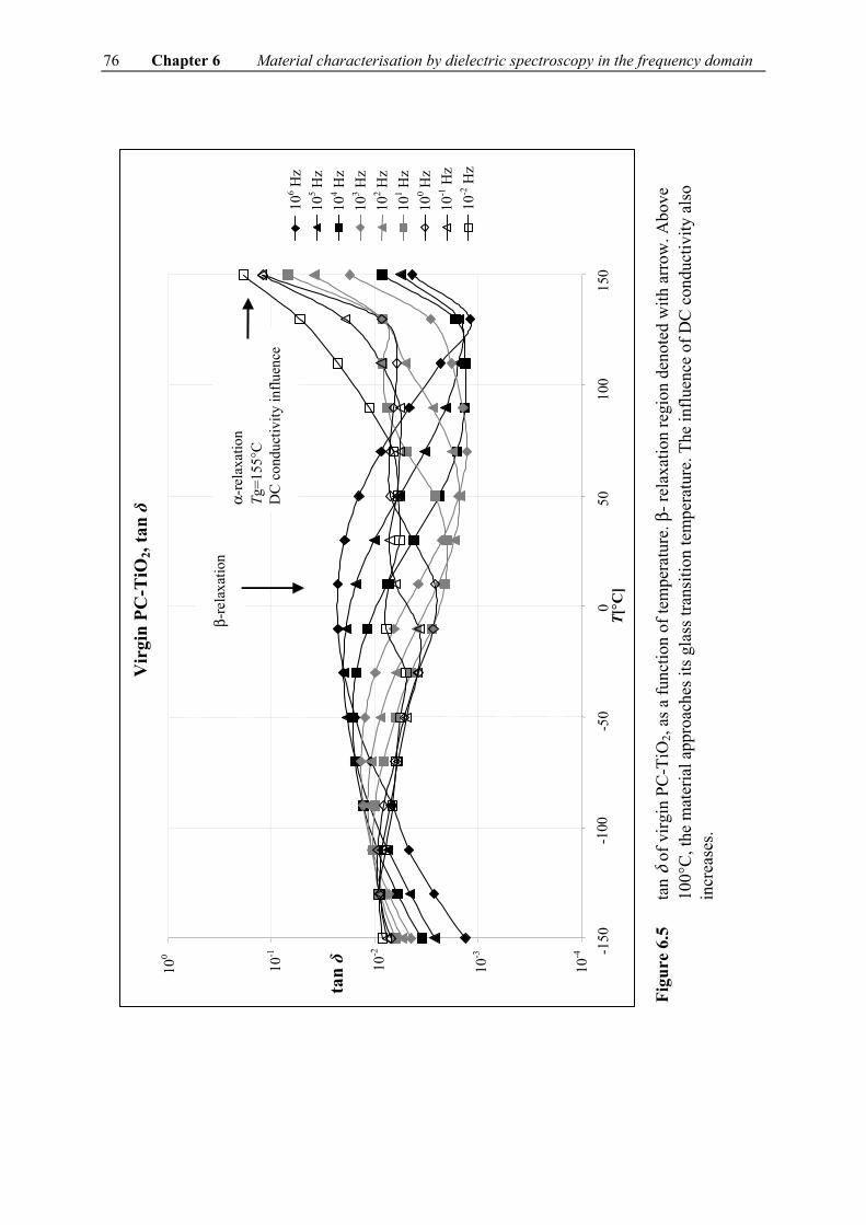
76 Chapter 6 Material characterisation by dielectric spectroscopy in the frequency domain
Figu
re 6
.5
tan
δ of
virg
in P
C-T
iO2,
as a
func
tion
of te
mpe
ratu
re. β
- rel
axat
ion
regi
on d
enot
ed w
ith a
rrow
. Abo
ve
100°
C, t
he m
ater
ial a
ppro
ache
s its
gla
ss tr
ansi
tion
tem
pera
ture
. The
influ
ence
of D
C c
ondu
ctiv
ity a
lso
incr
ease
s.
106 H
z 10
5 Hz
104 H
z 10
3 Hz
102 H
z 10
1 Hz
100 H
z 10
-1 H
z 10
-2 H
z
-150
-1
00
-50
0 50
10
0 15
0 T[
°C]
10-4
10-3
10-2
10-1
tan δ
100
Vir
gin
PC-T
iO2,
tan δ α-
rela
xatio
n Tg
=155
°C
DC
con
duct
ivity
influ
ence
β-re
laxa
tion

Material characterisation by dielectric spectroscopy in the frequency domain Chapter 6 77
106 H
z 10
5 Hz
104 H
z 10
3 Hz
102 H
z 10
1 Hz
100 H
z 10
-1 H
z 10
-2 H
z
-150
-1
00
-50
0 50
10
0 15
0 10
-4
10-3
10-2
10-1
tan δ
100
Pre-
stre
ssed
PC
-TiO
2, ta
n δ
β-re
laxa
tion
α-re
laxa
tion
Tg=1
55°C
D
C c
ondu
ctiv
ity in
fluen
ce
T[°C
]
Figu
re 6
.6
tan
δ of
pre
-stre
ssed
PC
-TiO
2, as
a fu
nctio
n of
tem
pera
ture
.β- r
elax
atio
n re
gion
den
oted
with
arr
ow.
Abo
ve 1
00°C
, the
mat
eria
l app
roac
hes i
ts g
lass
tran
sitio
n te
mpe
ratu
re. T
he in
fluen
ce o
f DC
con
duct
ivity
al
so in
crea
ses.

78 Chapter 6 Material characterisation by dielectric spectroscopy in the frequency domain
Figure 6.7 A typical β-relaxation detected in virgin PC-TiO2. The relaxation is
symmetrical, several decades wide, and its peak moves to higher temperatures as the frequency is increased.
Arrhenius plots of β-relaxations are given in Figure 6.8 and Figure 6.9. In a semi-log plot of the position of the β relaxation peak versus 1000/T, the experimental data can be fitted along a straight line, which supports the assumption of the Arrhenius process. The activation energies calculated from the slope of the Arrhenius plot are Wa = 2.18 eV for the virgin material, and Wa = 2.27 eV for the pre-stressed material. Pre-stressing the material has evidently not resulted in a significant change of temperature dependency in the side chain relaxation processes.
Virgin PC-TiO2, tan δ
10-4
10-3
10-2
10-1
100
-150 -100 -50 0 50 100 150
T [°C]
tan
δ
106 Hz 104 Hz 102 Hz
β-relaxation shift

Material characterisation by dielectric spectroscopy in the frequency domain Chapter 6 79
Figure 6.8 Arrhenius plot of virgin PC-TiO2: location of β-relaxation versus 1/T. Activation energy of the β-relaxation calculated from the slope: Wa = 2.18 eV.
Figure 6.9 Arrhenius plot of pre-stressed PC-TiO2: location of β-relaxation versus 1/T. Activation energy of the β-relaxation calculated from the slope: Wa = 2.27 eV.
In the high-temperature region, 50°C … 150°C, α-relaxation was detected, superimposed on the contribution of the conductivity to tan δ, as mentioned at the beginning of this sub-section. In Figure 6.10, ε″ is plotted against temperature for a frequency of 10 Hz, between 140°C and 200°C. The measurement was performed according to Procedure 2: ε″ was measured at a
Virgin PC-TiO2, Arrhenius plot
y = -2.18x + 13.84 R2 = 0.9822
1000/T [1/K] 3 4 5 6 7 8
-4
-2
0
2
4
6
8 lo
g f [
Hz]
Pre-stressed PC-TiO2, Arrhenius plot
y = -2.27x + 14.38 R2 = 0.9809
1000/T [1/K] 3 4 5 6 7 8
-4
-2
0
2
4
6
8
log
f [H
z]

80 Chapter 6 Material characterisation by dielectric spectroscopy in the frequency domain
constant temperature increase. The α-relaxation peak is detected slightly above the glass transition point. The increasing contribution of DC conductivity to the loss factor with temperature is also clearly visible. The contribution of DC conduction is predominantly observable above the glass-transition temperature Tg, and often obscures loss peaks of dipolar origin [63]. The effect of DC conductivity σDC on ε″ is easily seen from equation (6.3):
( ) ( )pol0
dcσε ω ε ωε ω
′′ ′′= + (6.3)
where ε″pol(ω) accounts for the losses of dipolar origin. The second term in the equation may be obtained using one of the Kramers-Kronig relations:
( ) ( ) 2 20
2 dωε ω ε ω ωπ ω ω
∞′′ ′ ′=
′ −∫ (6.4)
According to equation (6.3), the effect of DC conductivity will show up as a linear increase of ε ′′ with decreasing frequency. Using the DC conductivities reported in [24], an indication of the effect of σDC on ε″ is obtained. Extrapolation of the data results in σDC = 6.7 × 10⁻¹² S/m for virgin PC-TiO2 at 150°C and 25 kV/mm. Filling in the data in the first term of (6.3) leads to:
f.
f..
ωεσDC 120
2108581076
12
12
0=
π⋅⋅⋅=
−
−
At a frequency of 10 Hz the contribution of the first term in (6.3) is: σDC /ε0ω = 1.2×10⁻². Obviously, σDC /ε0ω accounts for a considerable share in the imaginary part of complex permittivity of PC-TiO2, which according to Figure 6.10 is: ε″ = 7×10⁻² at T = 150°C and f = 10 Hz.
Virgin PC-TiO2, f = 10 Hz
10-3
10-2
10-1
1
140 150 160 170 180 190 200 T [°C]
ε"
conductivity contribution
Tg= 155°C
α-relaxation peak
Figure 6.10 Virgin PC-TiO2: α-relaxation close to the glass transition point at 155ºC,
measurement performed at 10 Hz. The contribution of conductivity is particularly visible at higher temperatures.
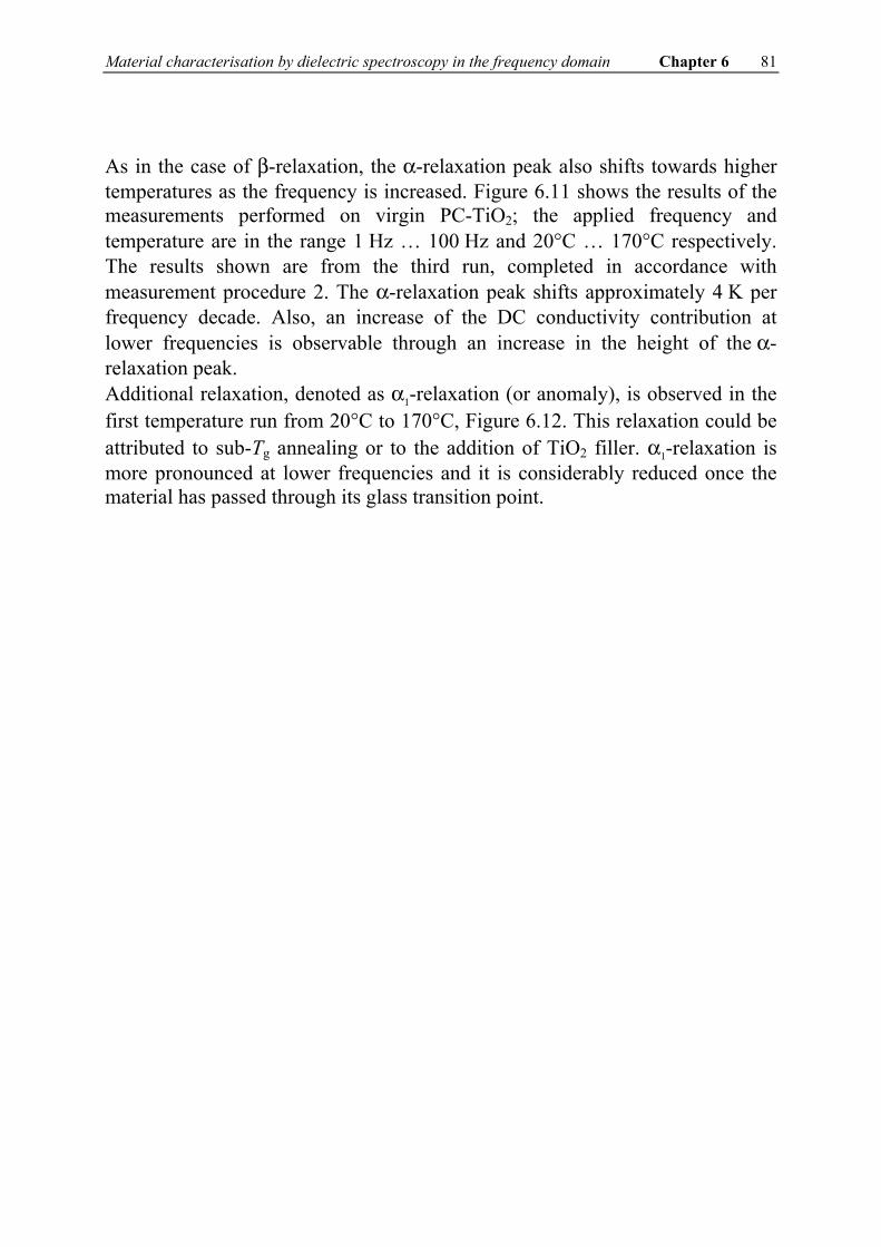
Material characterisation by dielectric spectroscopy in the frequency domain Chapter 6 81
As in the case of β-relaxation, the α-relaxation peak also shifts towards higher temperatures as the frequency is increased. Figure 6.11 shows the results of the measurements performed on virgin PC-TiO2; the applied frequency and temperature are in the range 1 Hz … 100 Hz and 20°C … 170°C respectively. The results shown are from the third run, completed in accordance with measurement procedure 2. The α-relaxation peak shifts approximately 4 K per frequency decade. Also, an increase of the DC conductivity contribution at lower frequencies is observable through an increase in the height of the α-relaxation peak. Additional relaxation, denoted as α1-relaxation (or anomaly), is observed in the first temperature run from 20°C to 170°C, Figure 6.12. This relaxation could be attributed to sub-Tg annealing or to the addition of TiO2 filler. α1-relaxation is more pronounced at lower frequencies and it is considerably reduced once the material has passed through its glass transition point.

82 Chapter 6 Material characterisation by dielectric spectroscopy in the frequency domain
Figure 6.11 Virgin PC-TiO2 Run 3: α-relaxation close to the glass transition point at 155ºC,
measurement performed at 1 Hz, 10 Hz and 100 Hz. Applied procedure: Run 1 20°C…170°C; Run 2 170°C…20°C; Run 3 20°C…170°C.
Figure 6.12 Virgin PC-TiO2, Run 1 20°C…170°C: α-relaxation close to the glass
transition point at 155ºC and α1-relaxation as a consequence of sub-Tg annealing or possibly due to the addition of TiO2 filler.
Virgin PC-TiO2, run 3
20 40 60 80 100 120 140 160 180T [°C]
0
5
10
15
20
25
30
35 ta
n δ
x 10
-3
1 Hz 10 Hz 100 Hz
increase of α-relaxation peak due to increased DC conductivity
Virgin PC-TiO2, run 1
20 40 60 80 100 120 140 160 180T [°C]
0
5
10
15
20
25
30
35
tan
δ x
10-3
1 Hz 10 Hz 100 Hz
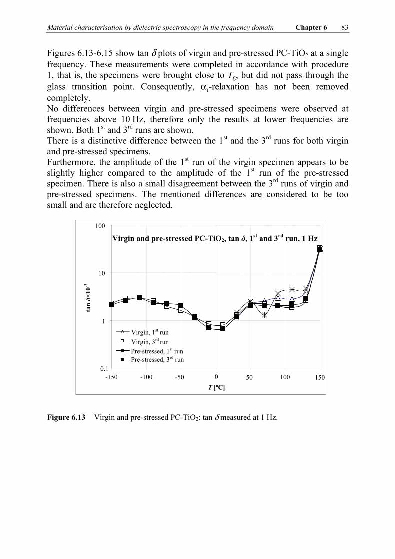
Material characterisation by dielectric spectroscopy in the frequency domain Chapter 6 83
Figures 6.13-6.15 show tan δ plots of virgin and pre-stressed PC-TiO2 at a single frequency. These measurements were completed in accordance with procedure 1, that is, the specimens were brought close to Tg, but did not pass through the glass transition point. Consequently, α1-relaxation has not been removed completely. No differences between virgin and pre-stressed specimens were observed at frequencies above 10 Hz, therefore only the results at lower frequencies are shown. Both 1st and 3rd runs are shown. There is a distinctive difference between the 1st and the 3rd runs for both virgin and pre-stressed specimens. Furthermore, the amplitude of the 1st run of the virgin specimen appears to be slightly higher compared to the amplitude of the 1st run of the pre-stressed specimen. There is also a small disagreement between the 3rd runs of virgin and pre-stressed specimens. The mentioned differences are considered to be too small and are therefore neglected. Figure 6.13 Virgin and pre-stressed PC-TiO2: tan δ measured at 1 Hz.
0.1
1
10
100
-150 -100 -50 0 T [ºC]
tan δ×
10-3
Virgin, 1st run Virgin, 3rd run
- Pre-stressed, 1st run Pre-stressed, 3rd run
50 100 150
Virgin and pre-stressed PC-TiO2, tan δ, 1st and 3rd run, 1 Hz

84 Chapter 6 Material characterisation by dielectric spectroscopy in the frequency domain
Figure 6.14 Virgin and pre-stressed PC-TiO2: tan δ measured at 0.1 Hz.
Figure 6.15 Virgin and pre-stressed PC-TiO2: tan δ measured at 0.01 Hz.
Virgin and pre-stressed PC-TiO2, tan δ, 1st and 3rd run, 0.1Hz
0.1
1
10
100
-150 -100 -50 0 50 100 150T [ºC]
tan δ×
10-3
Virgin, 1st runVirgin, 3rd runPre-stressed, 1st runPre-stressed, 3rd run
Virgin and pre-stressed PC-TiO2, tan δ, 1st and 3rd run, 0.01 Hz
0.1
1
10
100
-150 -100 -50 0 50 100 150T [ºC]
tan δ
×10-3
Virgin, 3rd runPre-stressed, 3rd runVirgin, 1st runPre-stressed, 1st run

Material characterisation by dielectric spectroscopy in the frequency domain Chapter 6 85
6.2.2 Real part of complex permittivity
The real parts of complex permittivity of virgin and pre-stressed PC-TiO2 as a function of temperature are given in Figure 6.16 and Figure 6.17 respectively.
Figure 6.16 Real part of complex permittivity of virgin PC-TiO2 as a function of
temperature.
Figure 6.17 Real part of complex permittivity of pre-stressed PC-TiO2 as a function of
temperature. The real part of complex permittivity of pre-stressed PC-TiO2 is approximately 10 % lower than that for new PC-TiO2 over the investigated frequency and
Pre-stressed PC-TiO2, ε΄
2.5
3.0
3.5
4.0
4.5
ε΄
-150 -100 -50 0 50 100 150 T [°C]
106 Hz 105 Hz 104 Hz 103 Hz 102 Hz 101 Hz 100 Hz 10-1 Hz 10-2 Hz
-150 2.5
3.0
3.5
4.0
4.5
ε΄
106 Hz 105 Hz 104 Hz 103 Hz 102 Hz 101 Hz 100 Hz 10-1 Hz 10-2 Hz
-100 -50 0 50 100 150
Virgin PC-TiO2, ε΄
T [°C]
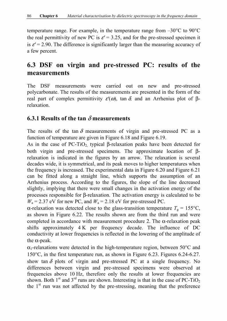
86 Chapter 6 Material characterisation by dielectric spectroscopy in the frequency domain
temperature range. For example, in the temperature range from –30°C to 90°C the real permittivity of new PC is ε′ = 3.25, and for the pre-stressed specimen it is ε′ = 2.90. The difference is significantly larger than the measuring accuracy of a few percent.
6.3 DSF on virgin and pre-stressed PC: results of the measurements
The DSF measurements were carried out on new and pre-stressed polycarbonate. The results of the measurements are presented in the form of the real part of complex permittivity ε′(ω), tan δ, and an Arrhenius plot of β-relaxation.
6.3.1 Results of the tan δ measurements
The results of the tan δ measurements of virgin and pre-stressed PC as a function of temperature are given in Figure 6.18 and Figure 6.19. As in the case of PC-TiO2, typical β-relaxation peaks have been detected for both virgin and pre-stressed specimens. The approximate location of β-relaxation is indicated in the figures by an arrow. The relaxation is several decades wide, it is symmetrical, and its peak moves to higher temperatures when the frequency is increased. The experimental data in Figure 6.20 and Figure 6.21 can be fitted along a straight line, which supports the assumption of an Arrhenius process. According to the figures, the slope of the line decreased slightly, implying that there were small changes in the activation energy of the processes responsible for β-relaxation. The activation energy is calculated to be Wa = 2.37 eV for new PC, and Wa = 2.18 eV for pre-stressed PC. α-relaxation was detected close to the glass-transition temperature Tg = 155°C, as shown in Figure 6.22. The results shown are from the third run and were completed in accordance with measurement procedure 2. The α-relaxation peak shifts approximately 4 K per frequency decade. The influence of DC conductivity at lower frequencies is reflected in the lowering of the amplitude of the α-peak. α1-relaxations were detected in the high-temperature region, between 50°C and 150°C, in the first temperature run, as shown in Figure 6.23. Figures 6.24-6.27. show tan δ plots of virgin and pre-stressed PC at a single frequency. No differences between virgin and pre-stressed specimens were observed at frequencies above 10 Hz, therefore only the results at lower frequencies are shown. Both 1st and 3rd runs are shown. Interesting is that in the case of PC-TiO2 the 1st run was not affected by the pre-stressing, meaning that the preference

Material characterisation by dielectric spectroscopy in the frequency domain Chapter 6 87
direction due to production process remained preserved. In contrast to this, the 1st run of pre-stressed PC is totally different from the 1st run of a virgin specimen: the pre-stressing erased “material memory”.
Figu
re 6
.18
tan δ
of v
irgin
PC
as a
func
tion
of te
mpe
ratu
re. D
etec
ted
β lo
ss p
eaks
mov
e to
hig
her
tem
pera
ture
s as t
he fr
eque
ncy
is in
crea
sed.
Vir
gin
PC, t
an δ
10-4
10-3
10-2
10-1
100 -1
50
-100
-5
0 0
50
100
150
106 H
z 10
5 Hz
104 H
z 10
3 Hz
102 H
z 10
1 Hz
100 H
z 10
-1 H
z 10
-2 H
z
tan δ
T [°
C]
β-re
laxa
tion
α-re
laxa
tion,
Tg=
155°
C
influ
ence
of D
C c
ondu
ctiv
ity

88 Chapter 6 Material characterisation by dielectric spectroscopy in the frequency domain
Figu
re 6
.19
tan δ
of p
re-s
tress
ed P
C a
s a fu
nctio
n of
tem
pera
ture
.
Det
ecte
d β
loss
pea
ks m
ove
to h
ighe
r tem
pera
ture
s as t
he fr
eque
ncy
is in
crea
sed.
106 H
z 10
5 Hz
104 H
z 10
3 Hz
102 H
z 10
1 Hz
100 H
z 10
-1 H
z 10
-2 H
z
-150
-1
00
-50
0 50
10
0 15
0 T
[C]
10-4
10-3
10-2
10-1
100
tan δ
Pre-
stre
ssed
PC
, tan
δ
α-re
laxa
tion
influ
ence
of D
C c
ondu
ctiv
ity
β-re
laxa
tion
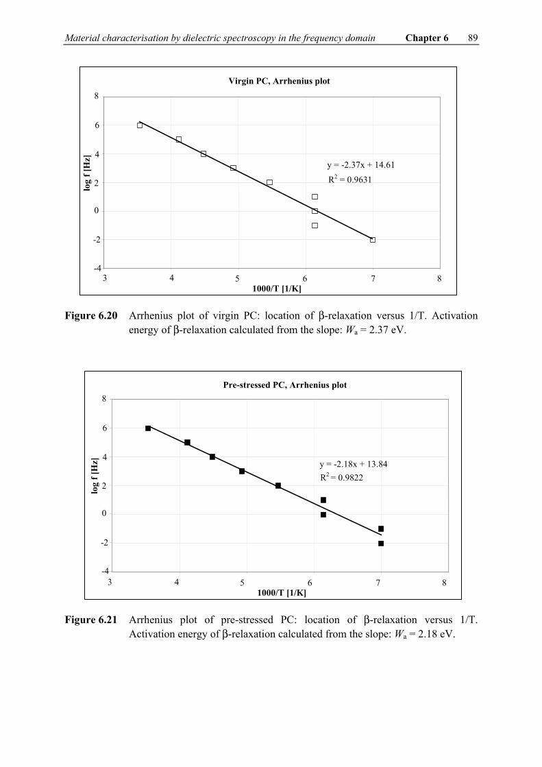
Material characterisation by dielectric spectroscopy in the frequency domain Chapter 6 89
Figure 6.20 Arrhenius plot of virgin PC: location of β-relaxation versus 1/T. Activation
energy of β-relaxation calculated from the slope: Wa = 2.37 eV.
Figure 6.21 Arrhenius plot of pre-stressed PC: location of β-relaxation versus 1/T.
Activation energy of β-relaxation calculated from the slope: Wa = 2.18 eV.
Virgin PC, Arrhenius plot
y = -2.37x + 14.61 R2 = 0.9631
-4
-2
0
2
4
6
8
1000/T [1/K]
log
f [H
z]
3 4 5 6 7 8
Pre-stressed PC, Arrhenius plot
y = -2.18x + 13.84 R2 = 0.9822
1000/T [1/K] 3 4 5 6 7 8
-4
-2
0
2
4
6
8
log
f [H
z]

90 Chapter 6 Material characterisation by dielectric spectroscopy in the frequency domain
Figure 6.22 Virgin PC, Run 3: α-relaxation close to the glass transition point at 155ºC,
measurement performed at 1 Hz, 10 Hz and 100 Hz. Applied procedure: Run 1 20°C…170°C; Run 2 170°C…20°C; Run 3 20°C…170°C.
Figure 6.23 Virgin PC, Run 1 20°C…170°C: α-relaxation close to the glass transition
point at 155ºC and α1-relaxation as a consequence of a sub-Tg annealing.
Virgin PC, run 1
0
5
10
15
20
25
30
35
20 40 60 80 100 120 140 160 180T [°C]
tan
δ ×
10-3
1 Hz10 Hz 100 Hz
Virgin PC, run 3
20 40 60 80 100 120 140 160 180T [°C]
0
5
10
15
20
25
30
35 ta
n δ
× 10
-3
1 Hz 10 Hz 100 Hz
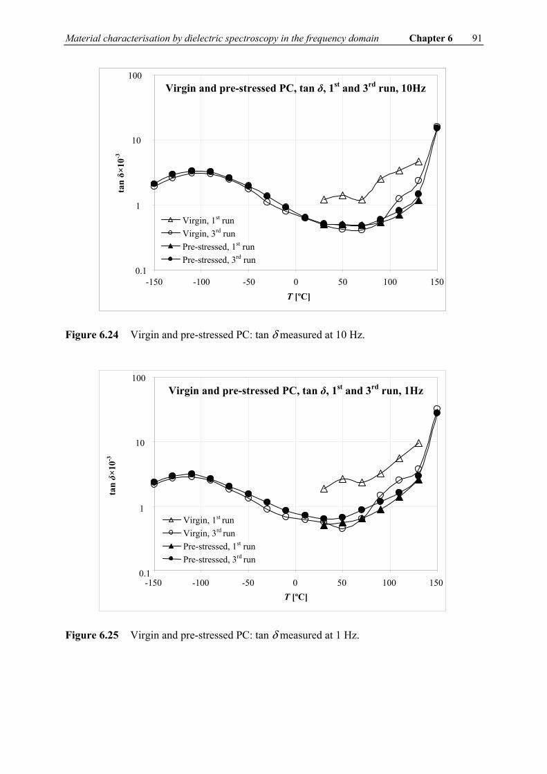
Material characterisation by dielectric spectroscopy in the frequency domain Chapter 6 91
Figure 6.24 Virgin and pre-stressed PC: tan δ measured at 10 Hz.
Figure 6.25 Virgin and pre-stressed PC: tan δ measured at 1 Hz.
Virgin and pre-stressed PC, tan δ, 1st and 3rd run, 10Hz
0.1
1
10
100
-150 -100 -50 0 50 100 150T [ºC]
tan δ×
10-3
Virgin, 1st runVirgin, 3rd runPre-stressed, 1st runPre-stressed, 3rd run
Virgin and pre-stressed PC, tan δ, 1st and 3rd run, 1Hz
T [ºC]
Virgin, 1st runVirgin, 3rd runPre-stressed, 1st runPre-stressed, 3rd run
-150 -100 -50 0 50 100 1500.1
1
10
100
tan δ×
10-3
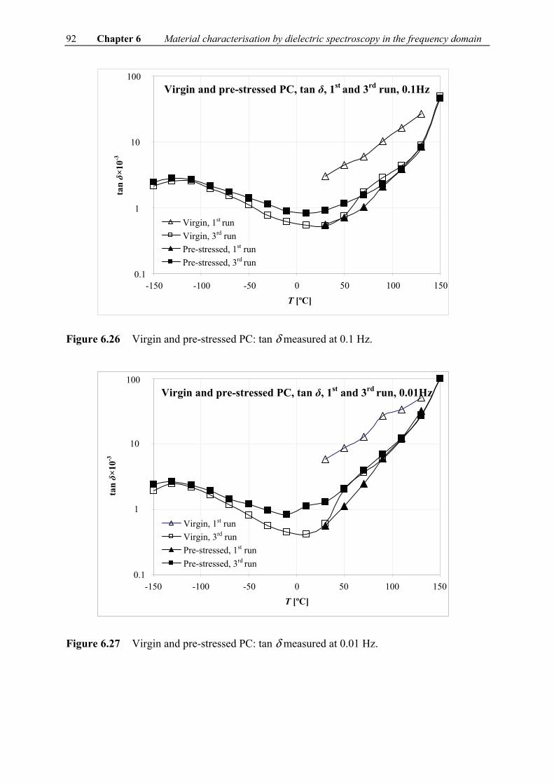
92 Chapter 6 Material characterisation by dielectric spectroscopy in the frequency domain
Figure 6.26 Virgin and pre-stressed PC: tan δ measured at 0.1 Hz.
Figure 6.27 Virgin and pre-stressed PC: tan δ measured at 0.01 Hz.
Virgin and pre-stressed PC, tan δ, 1st and 3rd run, 0.1Hz
-150 -100 -50 0 50 100 150T [ºC]
Virgin, 1st runVirgin, 3rd runPre-stressed, 1st runPre-stressed, 3rd run
0.1
1
10
100
tan δ×
10-3
Virgin and pre-stressed PC, tan δ, 1st and 3rd run, 0.01Hz
-150 -100 -50 0 50 100 150T [ºC]
Virgin, 1st runVirgin, 3rd runPre-stressed, 1st runPre-stressed, 3rd run
0.1
1
10
100
tan δ×
10-3

Material characterisation by dielectric spectroscopy in the frequency domain Chapter 6 93
6.3.2 Real part of complex permittivity
The real part of complex permittivity as a function of temperature for virgin and pre-stressed PC is given in Figure 6.28 and Figure 6.29.
Figure 6.28 Real part of complex permittivity of virgin PC as a function of temperature.
Figure 6.29 Real part of complex permittivity of pre-stressed PC as a function of temperature.
The real part of complex permittivity of pre-stressed PC is higher than that of virgin material in the whole frequency range for each temperature. For example, in the temperature range between -30°C and 90°C the real permittivity of new PC is ε′ = 2.60, and for the pre-stressed specimen it is ε′ = 2.90.
Virgin PC, ε΄
2.0
2.5
3.0
3.5
4.0
ε΄
106 Hz 105 Hz 104 Hz 103 Hz 102 Hz 101 Hz 100 Hz 10-1 Hz 10-2 Hz
-150 -100 -50 0 50 100 150 T [°C]
Pre-stressed PC, ε΄
2.0
2.5
3.0
3.5
4.0
ε΄
-150 -100 -50 0 50 100 150 T [°C]
106 Hz 105 Hz 104 Hz 103 Hz 102 Hz 101 Hz 100 Hz 10-1 Hz 10-2 Hz
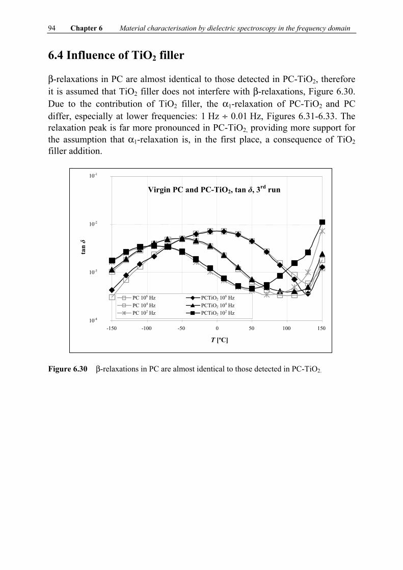
94 Chapter 6 Material characterisation by dielectric spectroscopy in the frequency domain
6.4 Influence of TiO2 filler
β-relaxations in PC are almost identical to those detected in PC-TiO2, therefore it is assumed that TiO2 filler does not interfere with β-relaxations, Figure 6.30. Due to the contribution of TiO2 filler, the α1-relaxation of PC-TiO2 and PC differ, especially at lower frequencies: 1 Hz ÷ 0.01 Hz, Figures 6.31-6.33. The relaxation peak is far more pronounced in PC-TiO2, providing more support for the assumption that α1-relaxation is, in the first place, a consequence of TiO2 filler addition. Figure 6.30 β-relaxations in PC are almost identical to those detected in PC-TiO2.
Virgin PC and PC-TiO2, tan δ, 3rd run
10-4
10-3
10-2
10-1
-150 -100 -50 0 50 100 150 T [ºC]
tan δ
PC 106 Hz PCTiO2 106 HzPC 104 Hz PCTiO2 104 HzPC 102 Hz PCTiO2 102 Hz

Material characterisation by dielectric spectroscopy in the frequency domain Chapter 6 95
Figure 6.31 Virgin PC and PC-TiO2: tan δ measured at 100 Hz. Figure 6.32 Virgin PC and PC-TiO2: tan δ measured at 1 Hz.
Virgin PC and PC-TiO2, tan δ, 3rd run
10-4
10-3
10-2
10-1
-150 -100 -50 0 50 100 150 T [ºC]
tan δ
PC 102 Hz
PC-TiO2 102 Hz
Virgin PC and PC-TiO2, tan δ, 3rd run
10-4
10-3
10-2
10-1
-150 -100 -50 0 50 100 150 T [ºC]
tan δ
PC 1 Hz
PC-TiO2 1 Hz

96 Chapter 6 Material characterisation by dielectric spectroscopy in the frequency domain
Figure 6.33 Virgin PC and PC-TiO2: tan δ measured at 0.01 Hz. Figures 6.34-6.36 present tan δ of virgin PC and PC-TiO2 measured between 20°C and 170°C in Run 3, that is, after the specimens have already passed through the glass transition point once. tan δ of PC-TiO2 specimens is higher than that of PC, exactly in the region where α1-relaxation was detected in Run 1. This is one more indication that TiO2 filler has a considerable contribution to α1-relaxation.
Virgin PC and PC-TiO2, tan δ, 3rd run
10-4
10-3
10-2
10-1
-150 -100 -50 0 50 100 150 T [ºC]
tan δ
PC 10-2 Hz
PC-TiO2 10-2 Hz

Material characterisation by dielectric spectroscopy in the frequency domain Chapter 6 97
Figure 6.34 Virgin PC and PC-TiO2: tan δ measured at 1 Hz.
Figure 6.35 Virgin PC and PC-TiO2: tan δ measured at 10 Hz.
PC-TiO2 PC
Virgin PC & PC-TiO2 run 3, f = 10 Hz
20 40 60 80 100 120 140 160 180T [°C]
0
5
10
15
20
25
30
35
tan
δ ×
10-3
Virgin PC & PC-TiO2 run 3, f = 1 Hz
PC-TiO2 PC
20 40 60 80 100 120 140 160 180T [°C]
0
5
10
15
20
25
30
35 ta
n δ
× 10
-3
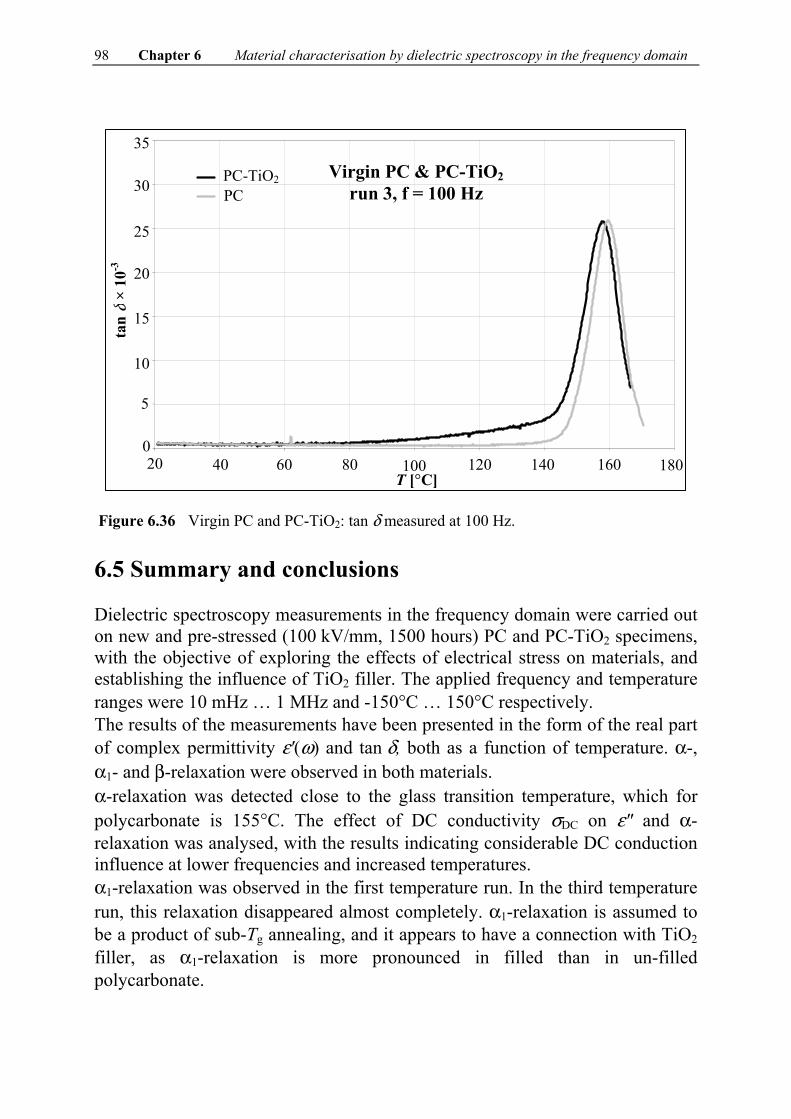
98 Chapter 6 Material characterisation by dielectric spectroscopy in the frequency domain
Figure 6.36 Virgin PC and PC-TiO2: tan δ measured at 100 Hz.
6.5 Summary and conclusions
Dielectric spectroscopy measurements in the frequency domain were carried out on new and pre-stressed (100 kV/mm, 1500 hours) PC and PC-TiO2 specimens, with the objective of exploring the effects of electrical stress on materials, and establishing the influence of TiO2 filler. The applied frequency and temperature ranges were 10 mHz … 1 MHz and -150°C … 150°C respectively. The results of the measurements have been presented in the form of the real part of complex permittivity ε′(ω) and tan δ, both as a function of temperature. α-, α1- and β-relaxation were observed in both materials. α-relaxation was detected close to the glass transition temperature, which for polycarbonate is 155°C. The effect of DC conductivity σDC on ε″ and α-relaxation was analysed, with the results indicating considerable DC conduction influence at lower frequencies and increased temperatures. α1-relaxation was observed in the first temperature run. In the third temperature run, this relaxation disappeared almost completely. α1-relaxation is assumed to be a product of sub-Tg annealing, and it appears to have a connection with TiO2 filler, as α1-relaxation is more pronounced in filled than in un-filled polycarbonate.
PC-TiO2 PC
Virgin PC & PC-TiO2 run 3, f = 100 Hz
20 40 60 80 100 120 140 160 180T [°C]
0
5
10
15
20
25
30
35 ta
n δ
× 10
-3

Material characterisation by dielectric spectroscopy in the frequency domain Chapter 6 99
To analyse the behaviour of β-relaxation, the activation energies were calculated from the slope of Arrhenius plots. The activation energy of β-relaxation in PC-TiO2 slightly increased due to pre-stressing: from 2.18 eV for virgin, to 2.27 eV for pre-stressed PC-TiO2. The opposite results were obtained for PC: the activation energy of β-relaxation in PC slightly decreased due to pre-stressing: from 2.37 eV for virgin, to 2.18 eV for pre-stressed PC. Pre-stressing materials has evidently not resulted in a significant change in the temperature dependency of the side chain relaxation processes. Comparable values of activation energies, as well as the almost identical shapes of β-relaxation in both materials, indicate that the addition of TiO2 filler has minor impact on side chain relaxation.
The real part of complex permittivity ε′(ω) increased as a consequence of pre-stressing from 2.60 for virgin PC, to 2.90 for pre-stressed PC, which has been interpreted as an increase of material polarisability. According to the Clausius-Mosotti equation, α polarisability increases with increases in the real part of complex permittivity ε′. The same interpretation does not hold true for pre-stressed PC-TiO2 as the real part of complex permittivity decreased from 3.25 in virgin material to 2.90 in pre-stressed material.

100 Chapter 6 Material characterisation by dielectric spectroscopy in the frequency domain

Breakdown tests Chapter 7 101
BBrreeaakkddoowwnn tteessttss 77
7.1 Introduction
The aim of the breakdown tests performed in the scope of the present research was twofold:
A number of breakdown tests were carried out on PC-TiO2 with the purpose of determining the life expectancy of the material when exposed to DC voltages. Only PC-TiO2 was tested in this way, assuming it to be a weaker material than pure PC because of the addition of filler. Based on the life expectancy characteristic obtained, an electrical field strength was chosen for artificial aging tests, which in this thesis is termed as pre-stressing.
A number of breakdown step-up tests were performed on new and pre-stressed PC and PC-TiO2 in order to compare the voltage endurance of the materials and the influence of pre-stressing on voltage endurance.

102 Chapter 7 Breakdown tests
7.2 Voltage endurance tests and pre-stress determination
Results of the breakdown tests are given in Figure 7.1. The voltage increase rate was 5 kV per minute up to the intended voltage, and the time to breakdown was measured. The number of tested samples for each field strength was as given in Table 7.1. Table 7.1 Field strengths (voltages) and number of tested samples, specimen thickness
0.175 mm. Field strength [kV/mm] Voltage [kV] Number of tested samples and status
171 30 3, breakdown within a couple of minutes 143 25 4, breakdown within one hour 114 20 2, no breakdown within 8 hours 46 8 16 (aging test), no breakdown after 3000 hours
Figure 7.1 Breakdown voltages versus field strengths and lifeline of PC-TiO2. Arrows
denote samples that have not broken-down: at 112 kV after 8 hours and at 46 kV/mm after 3000 hours.
All pre-stressed specimens analysed in this thesis were exposed to 100 kV/mm DC electrical stress, with the expectation that the specimens would be considerably aged after a couple of hundred hours. The majority of the test-specimens had not broken down by the time that the test was stopped, after 1500 hours.
time [hour]
100
30
40
50
60
70
80 90
200
elec
tric
field
stre
ngth
[kV
/mm
]
10-2 10-1 100 101 102 103 104 105 106

Breakdown tests Chapter 7 103
7.3 DC breakdown step-up tests
Breakdown step-up tests were performed on new and pre-stressed PC and PC-TiO2 specimens. At least four specimens were tested each time. The primary goal of the tests was to check if the stressed materials were indeed electrically aged. The secondary goal was a comparison of different materials. The rate of voltage increase was 1 kV/minute. Results of the step-up breakdown tests are given in Figure 7.2.
50
100
150
200
250
300
350
400
450
Bre
akdo
wn
stre
ss [k
V/m
m]
virgin PC pre-stressed PCvirgin PC-TiO2
pre-stressed PC-TiO2
PC PC-TiO2
virgin
virgin
pre-stressed
pre-stressed
test-specimen Figure 7.2 Results of the breakdown step-up tests on new and pre-stressed PC and PC-
TiO2. The breakdown strength of PC is considerably higher than that of PC-TiO2: between 450 kV/mm and 400 kV/mm for new PC, and between 200 kV/mm and 250 kV/mm for new PC-TiO2. Due to pre-stressing, the breakdown strength of PC is slightly decreased. Pre-stressing appears to have more influence on PC-TiO2: the breakdown strength decreased from between 200 kV/mm and 250 kV/mm, to approximately 170 kV/mm.
7.4 Summary
Two types of breakdown test were performed:
Voltage endurance test for pre-stress determination. Step-up breakdown test as a tool to compare PC and PC-TiO2, and to
determine the influence of pre-stressed material on voltage endurance.
104 Chapter 7 Breakdown tests
Based on the voltage endurance tests, a 100 kV/mm electrical DC stress was chosen as the level of pre-stressing to be applied to the materials used in this thesis. Step-up tests resulted in higher voltage endurance for PC than PC-TiO2. Voltage endurance of both PC and PC-TiO2 decreased due to pre-stressing, but PC-TiO2 was shown to be more influenced by pre-stressing than PC.

105 Chapter 7 Breakdown tests

106 Chapter 7 Breakdown tests
Discussion of the results Chapter 8 107
DDiissccuussssiioonn ooff tthhee rreessuullttss 88
8.1 Introduction
In the previous chapters, a number of material test techniques were applied to virgin and pre-stressed PC and PC-TiO2 with the objective of analysing the following aspects:
Material performance concerning measured/calculated quantities as listed below:
- Space charge related quantities - Dielectric relaxations, complex permittivity - Conduction current; transition field from linear to non-linear regime - Breakdown strength
Influence of 100 kV/mm DC – 1500 hours pre-stressing on above mentioned material parameters.
Influence of the addition of TiO2 on polycarbonate dielectric properties. The main objective of this chapter is to bring all the test techniques together, and to discuss the possibility of using them as a method for material ranking and for estimating influence of electrical stress on material performance.

108 Chapter 8 Discussion of the results
The structural overview of the chapter is given in Figure 8.1. Figure 8.1 Structural overview of Chapter 8.
Chapter 8 Discussion of the results
8.1 Introduction
8.3 Discussion and
conclusions
8.2 Summary and discussion of the results
8.2.1 Space charge measurements
Influence of interfacial polarisation
Space charge quantities
Influence of the TiO2 filler
8.2.3 Dielectric spectroscopy in the
frequency domain
Results of tan δ measurements
8.2.2 Polarization current
measurements
E vs. Icon characteristic
8.2.4 Breakdown tests
Influence of the TiO2 filler
Influence of the TiO2 filler
Results of ε’ measurements

Discussion of the results Chapter 8 109
8.2 Summary and discussion of the measurement results
8.2.1 Space charge measurements
Space charge measurements were carried out on virgin and pre-stressed PC and PC-TiO2 specimens, applying electric fields in the range 1.7 kV/mm … 45.7 kV/mm. In processing the results of the space charge measurements, special attention is paid to the influence of the oil layer used to improve the acoustical coupling between the test specimens and the electrodes. A summary of the findings concerning the space charge related quantities of both materials is presented, as well as the influence of TiO2 filler. Influence of interfacial polarisation Figure 8.2 shows a measurement performed on virgin PC. A charging field of 1 kV/mm was applied for 3 hours, and at this field, PC is not supposed to accumulate any space charge1. The charge profile signal after switching off the poling voltage is therefore expected to be identical to the signal obtained before poling began, in other words identical to the response of the electrodes to the short high-voltage pulse. The response of the electrodes to the short high-voltage PEA pulse prior to poling is shown by the thick black line in Figure 8.2. The other signals given in the figure represent voltage-off signals measured from 9 seconds after switching-off the poling voltage until the moment that the voltage-off signal reached the value of the electrodes’ response, which was after approximately 100 s. Explanation for the observed mismatch between the electrode response and voltage-off signal of a specimen that accumulates no space charge at a given poling field is based on Maxwell-Wagner polarisation which predicts the formation of an induced surface charge at the oil-PC interface. The conductivity of the thin-oil layer is much larger than that of the dielectric specimen. Consequently, a surface charge is formed at the oil-dielectric interface, and the oil-layer acts as an electrode towards the dielectric. This can also be seen from the result of the calculation of the charge collected at the interface (8.1) [7]:
b a a bs
a b
K Ub a
σ ε σ εσ σ
−=+
(8.1)
1 The assumption that the tested specimen accumulates no space charge at the applied 1 kV/mm poling field is based on the results of conductivity current measurements (Chapter 5). The linear relationship between current and voltage up to 5.7 kV/mm indicates that no presence of space charge at that field strength should be expected.
110 Chapter 8 Discussion of the results
Where U is the applied voltage, σa and σb are conductivities of involved materials, εa and εb their permittivities and a and b are the thickness of material a and b. Filling in the data listed below [7], [11]: σoil = [1×10-12, 1×10-14 ][1/Ωm]; ε r,oil= 2.7; doil=15×10-6 [m] σPC= 6.4×10⁻¹⁸ [1/Ωm]; ε r,PC= 3.1; dPC=175×10-6 [m] and simplifying (8.1) by using σPC << σoil, the charge at the oil-PC interface at 1 kV/mm is calculated by:
427.4*10oil PC PC oil PCs
oil PC PC oil PC
K U Ud d dσ ε σ ε ε
σ σ−−= ≈ =
+[μC/cm2]
The time constant of the oil-PC interface polarisation is given by (8.2) [7]:
a b
a b
b ab a
ε ετσ σ
+=+
(8.2)
Using dPC>> doil, expression (8.2) can be simplified:
oil PC PC oil oil
oil PC PC oil oil
d dd d
ε ε ετσ σ σ
+= ≈+
(8.3)
The time constant is calculated to be in the range [24 s, 2400 s] for σoil = [1×10-12, 1×10-14 ][1/Ωm]. Depletion of the oil-PC interface proceeds, even in the most rapid case, in accordance with the same time constant. In this work, the time constant used is 250 s. The space charge density is therefore not calculated from the first voltage-off signal, but 5 time constants later, namely 1250 s.

Discussion of the results Chapter 8 111
Figure 8.2 Virgin PC, voltage-off signal after 3 hours poling at 1 kV/mm. The electrode
response signal prior to poling is given by the thick black line. Space charge quantities In all test-specimens, homo-charge was detected in the vicinity of the electrodes. In addition, in pre-stressed PC-TiO2, hetero-charge was also detected. An overview of the field enhancement factors obtained at a 32 kV/mm poling field is given in Table 8.1. The same is illustrated in Figure 8.3. Pre-stressing PC resulted in a higher bulk field enhancement, whereas field lowering in the proximity of the electrodes decreased. A higher field enhancement in the bulk was explained by a possible increase of trapping sites due to pre-stressing. The apparent improvement of pre-stressed PC-TiO2 concerning internal field enhancement was explained by the occurrence of hetero-charge, which compensates for the effect of homo-charge. An overview of the electrical threshold fields for space charge accumulation in virgin and pre-stressed specimens is given in Table 8.2. The same is illustrated in Figure 8.4. Table 8.1 Overview of the field enhancement factors in virgin and pre-stressed specimens. PC PC-TiO2
Virgin Electrode proximity: -43.7 % Bulk: 3.1 %
Electrode proximity: -44 % Bulk: 9.9 %
Pre-stressed
Electrode proximity: -37.5 % Bulk: 9.9 %
Electrode proximity: -18.7 % Bulk: 2.9 %
-0.8
-0.6
-0.4
-0.2
0
0.2
0.4
0.6
0.8
0 100 200 300 400measured points [number]
dete
cted
sign
al [m
V]
500
test specimenearth electrode
HV electrode
9
10
50
50
109
100

112 Chapter 8 Discussion of the results
Electrode proximity
Figure 8.3 Field enhancement factors at a poling field of 32 kV/mm. Table 8.2 Overview of the electrical threshold fields for space charge accumulation in
virgin and pre-stressed specimens. Poling field in the range 1.7 kV/mm … 45.7 kV/mm.
PC PCTiO2
Virgin 6.5 kV/mm 3.3 kV/mm < E th,sc <4.7 kV/mm
Pre-stressed
7 kV/mm < E th,sc < 13 kV/mm
2.8 kV/mm < E th,sc < 5.8 kV/mm
Figure 8.4 Electrical threshold fields of virgin and pre-stressed PC and PC-TiO2 test-
specimens are located in the shown ranges. The poling field was in the range of 1.7 kV/mm … 45.7 kV/mm.
Virgin PC Pre-stressed PC
Virgin PC-TiO2
Pre-stressed PC-TiO2
-43.7 %
-37.5 % -44 %
-18.7 %
9.9 %
9.9 %
3.1 %
2.9 %
Virgin PC Pre-stressed PC
Virgin PC-TiO2
Pre-stressed PC-TiO2
Bulk
10 5 15
pre-stressed PC
virgin PC
E [kV/mm]
10 15 0 5 virgin PC-TiO2
pre-stressed PC-TiO2
E [kV/mm]
0
Discussion of the results Chapter 8 113
The electrical threshold of PC remained the same or increased slightly due to pre-stressing. Similar was observed for PC-TiO2. In addition, the occurrence of hetero-charge in the pre-stressed PC-TiO2 test-specimens is believed to be the cause of the increased threshold. The accumulation process of both materials was described by two time constants. No relation was found with the applied field. τ1 measured for PC appears not to be influenced by pre-stressing. τ2 of PC, and τ1 and τ2 of PC-TiO2 were influenced by pre-stressing in ways that cannot be described analytically, but rather in the terms of less fluctuation or more fluctuation around a mean value. Influence of TiO2 filler on space-charge quantities The addition of TiO2 filler caused a lowering of the threshold field for space charge accumulation, which is not unexpected considering the fact that the filler introduced numerous interfaces at which space charge could accumulate. For the same reason, the field enhancement factor f is higher in the bulk of filled PC. In the proximity of the electrodes, surface defects are believed to prevail over the trapping sites introduced by the filler. Consequently, the filler traps caused no change in the field enhancement factor close to the electrodes.
8.2.2 Polarisation current measurements
Polarisation current measurements were performed on virgin and pre-stressed PC and PCTiO2 test-specimens, applying polarising fields in the range 1.7 kV/mm … 34.3 kV/mm. The values of the (estimated) conduction currents were plotted against the polarising fields in order to define a departure field from the linear (ohmic) regime, if any. E vs. Icon characteristic and electrical transition fields for conduction mechanisms Table 8.3 gives an overview of the electrical transition fields in virgin and pre-stressed specimens, showing the change in the slope of the E vs. Icon characteristic from a linear to a non-linear regime. The same is illustrated in Figure 8.5. A change of slope for the E vs. Icon characteristic from 1 to 2 was observed in all cases. This indicates a change in the conducting mechanism: from linear (ohmic) behaviour, where conduction is governed by surpassing the thermal activation energy level of the charge carrier out of trapping sites, to the point where the charge carrier’s mobility is increased to such an extent that the linear relationship does not hold any more.

114 Chapter 8 Discussion of the results
Table 8.3 Overview of the transition fields for the conduction mechanisms. PC PC-TiO2
Virgin 6 kV/mm 3 kV/mm
Pre-stressed < 3 kV/mm 3 kV/mm < E th,sc < 3.5 kV/mm
Figure 8.5 The electrical threshold fields of virgin and pre-stressed PC and PC-TiO2 test-
specimens are located in the shown ranges. The poling field was in the range 1.7 kV/mm … 45.7 kV/mm.
Influence of TiO2 filler on conduction current measurements The addition of TiO2 filler caused a lowering of the threshold field from 6 kV/mm in unfilled PC, to 3 kV/mm in filled PC.
8.2.3 Dielectric spectroscopy in frequency domain
Dielectric spectroscopy measurements in the frequency domain were performed on virgin and pre-stressed PC and PC-TiO2 specimens at the applied frequency and temperature ranges of 10 mHz … 1 MHz and -150°C … 150°C respectively. The effect of electrical stress on the materials was explored, as well as the effect of the addition of TiO2 filler to the molecular dynamics of the tested materials. Results of the tan δ measurements The following results were obtained from the tan δ characteristic plotted against temperature at different frequencies: α-, α1- and β-relaxation were observed in both materials.
0 10 5 15
pre-stressed PC virgin PC
E [kV/mm]
0 10 5 15 virgin PC-TiO2
pre-stressed PC-TiO2
E [kV/mm]
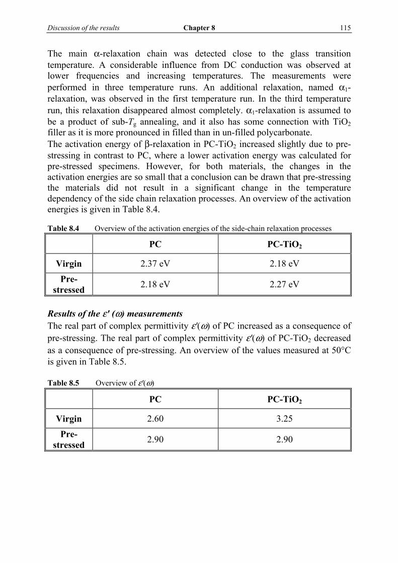
Discussion of the results Chapter 8 115
The main α-relaxation chain was detected close to the glass transition temperature. A considerable influence from DC conduction was observed at lower frequencies and increasing temperatures. The measurements were performed in three temperature runs. An additional relaxation, named α1-relaxation, was observed in the first temperature run. In the third temperature run, this relaxation disappeared almost completely. α1-relaxation is assumed to be a product of sub-Tg annealing, and it also has some connection with TiO2 filler as it is more pronounced in filled than in un-filled polycarbonate. The activation energy of β-relaxation in PC-TiO2 increased slightly due to pre-stressing in contrast to PC, where a lower activation energy was calculated for pre-stressed specimens. However, for both materials, the changes in the activation energies are so small that a conclusion can be drawn that pre-stressing the materials did not result in a significant change in the temperature dependency of the side chain relaxation processes. An overview of the activation energies is given in Table 8.4. Table 8.4 Overview of the activation energies of the side-chain relaxation processes PC PC-TiO2
Virgin 2.37 eV 2.18 eV
Pre-stressed 2.18 eV 2.27 eV
Results of the ε′ (ω) measurements The real part of complex permittivity ε′(ω) of PC increased as a consequence of pre-stressing. The real part of complex permittivity ε′(ω) of PC-TiO2 decreased as a consequence of pre-stressing. An overview of the values measured at 50°C is given in Table 8.5. Table 8.5 Overview of ε′(ω) PC PC-TiO2
Virgin 2.60 3.25
Pre-stressed 2.90 2.90

116 Chapter 8 Discussion of the results
Normally, a destructive stress would cause an increase of ε΄, being a measure of material polarisability. Indeed, this is observed in pre-stressed PC, but not in pre-stressed PC-TiO2. In this case a preference direction of the filler’s molecules induced by pre-stressing has not been removed by the hysteresis measurements (3 temperature runs). Influence of TiO2 filler The comparable values of the activation energies in virgin PC and PC-TiO2 specimens (2.37 eV and 2.18 eV), as well as the almost identical shape of β-relaxation in both materials, indicate that the addition of TiO2 filler has no impact on side chain relaxation. α1-relaxation was associated with TiO2 filler as it is more pronounced in filled than in un-filled polycarbonate. The addition of TiO2 resulted in a higher real part of complex permittivity.
8.2.4 Breakdown tests
Voltage endurance tests were performed with the objective of determining the pre-stress field. Based on the voltage endurance tests, a 100 kV/mm electrical DC stress was chosen as the level of pre-stressing to be applied to the materials used in this thesis. The results of step-up breakdown tests were used as tools to compare PC and PC-TiO2, and to determine the influence of pre-stressing on the voltage endurance of the tested materials. Step-up tests resulted in higher voltage endurance for PC than PC-TiO2. Evidently, the addition of TiO2 filler introduces numerous interfaces, which are always one of weakest points of insulation materials. Voltage endurance of both PC and PC-TiO2 slightly decreased due to pre-stressing, thereby PC-TiO2 was more influenced.
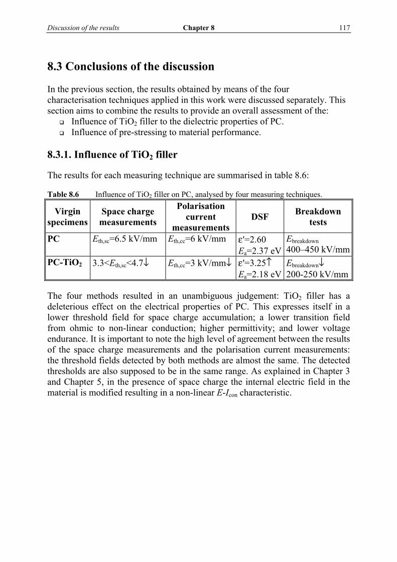
Discussion of the results Chapter 8 117
8.3 Conclusions of the discussion
In the previous section, the results obtained by means of the four characterisation techniques applied in this work were discussed separately. This section aims to combine the results to provide an overall assessment of the:
Influence of TiO2 filler to the dielectric properties of PC. Influence of pre-stressing to material performance.
8.3.1. Influence of TiO2 filler
The results for each measuring technique are summarised in table 8.6: Table 8.6 Influence of TiO2 filler on PC, analysed by four measuring techniques.
Virgin specimens
Space charge measurements
Polarisation current
measurements DSF Breakdown
tests
PC Eth,sc=6.5 kV/mm Eth,cc=6 kV/mm ε′=2.60 Ea=2.37 eV
Ebreakdown 400–450 kV/mm
PC-TiO2 3.3<Eth,sc<4.7↓ Eth,cc=3 kV/mm↓ ε′=3.25↑ Ea=2.18 eV
Ebreakdown↓ 200-250 kV/mm
The four methods resulted in an unambiguous judgement: TiO2 filler has a deleterious effect on the electrical properties of PC. This expresses itself in a lower threshold field for space charge accumulation; a lower transition field from ohmic to non-linear conduction; higher permittivity; and lower voltage endurance. It is important to note the high level of agreement between the results of the space charge measurements and the polarisation current measurements: the threshold fields detected by both methods are almost the same. The detected thresholds are also supposed to be in the same range. As explained in Chapter 3 and Chapter 5, in the presence of space charge the internal electric field in the material is modified resulting in a non-linear E-Icon characteristic.
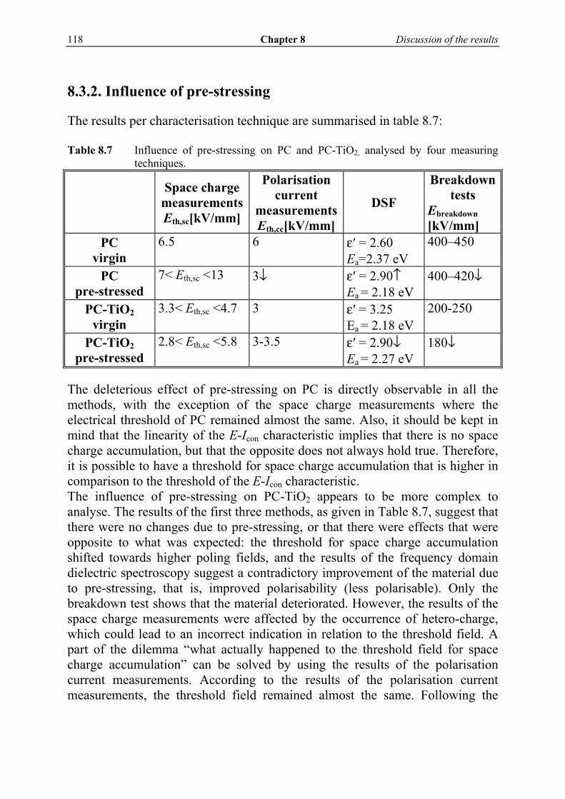
118 Chapter 8 Discussion of the results
8.3.2. Influence of pre-stressing
The results per characterisation technique are summarised in table 8.7: Table 8.7 Influence of pre-stressing on PC and PC-TiO2, analysed by four measuring
techniques.
Space charge
measurementsEth,sc[kV/mm]
Polarisation current
measurementsEth,cc[kV/mm]
DSF
Breakdown tests
Ebreakdown [kV/mm]
PC virgin
6.5 6 ε′ = 2.60 Ea=2.37 eV
400–450
PC pre-stressed
7< Eth,sc <13 3↓ ε′ = 2.90↑ Ea = 2.18 eV
400–420↓
PC-TiO2 virgin
3.3< Eth,sc <4.7 3 ε′ = 3.25 Ea = 2.18 eV
200-250
PC-TiO2 pre-stressed
2.8< Eth,sc <5.8 3-3.5 ε′ = 2.90↓ Ea = 2.27 eV
180↓
The deleterious effect of pre-stressing on PC is directly observable in all the methods, with the exception of the space charge measurements where the electrical threshold of PC remained almost the same. Also, it should be kept in mind that the linearity of the E-Icon characteristic implies that there is no space charge accumulation, but that the opposite does not always hold true. Therefore, it is possible to have a threshold for space charge accumulation that is higher in comparison to the threshold of the E-Icon characteristic. The influence of pre-stressing on PC-TiO2 appears to be more complex to analyse. The results of the first three methods, as given in Table 8.7, suggest that there were no changes due to pre-stressing, or that there were effects that were opposite to what was expected: the threshold for space charge accumulation shifted towards higher poling fields, and the results of the frequency domain dielectric spectroscopy suggest a contradictory improvement of the material due to pre-stressing, that is, improved polarisability (less polarisable). Only the breakdown test shows that the material deteriorated. However, the results of the space charge measurements were affected by the occurrence of hetero-charge, which could lead to an incorrect indication in relation to the threshold field. A part of the dilemma “what actually happened to the threshold field for space charge accumulation” can be solved by using the results of the polarisation current measurements. According to the results of the polarisation current measurements, the threshold field remained almost the same. Following the

Discussion of the results Chapter 8 119
same manner of interpretation as in the previous sub-section, the conclusion is that the threshold for space charge accumulation also remained the same.
8.3.3. Conclusions
With reference to the influence of TiO2 filler and pre-stressing on the dielectric properties of PC, the following is concluded:
TiO2 filler and pre-stressing have a deleterious effect on the electrical performance of PC.
The effect of pre-stressing on PC-TiO2 is difficult to analyse due to the occurrence of hetero-charge, and the quite complex role of the filler in relation to permittivity.
In seeking a suitable test method, which might consist of one or more measuring techniques, the following conclusions can be drawn:
Conduction current measurements and space charge measurements provide the same conclusion in relation to the threshold field of pure PC. However, space charge measurements provide more grounds for material characterisation. In this respect, conduction current analysis may be redundant as a test method. However, in analysing the influence of pre-stressing on filled PC, polarisation current measurements are still indispensable.
Dielectric spectroscopy in the frequency domain is a very powerful tool for material characterisation, providing a sensitive representation of material performance in a wide temperature and frequency range. This might not be so obvious in the cases of PC and PC-TiO2, but there are plenty of materials where the importance of using this method is more evident [50-53]. This technique should certainly be a part of a characterisation method.
Breakdown tests are inevitable for the ranking of HV insulating materials. They provide an indication of voltage endurance and life expectancy, which are often essential when choosing a suitable material.

120 Chapter 8 Discussion of the results
Conclusions and recommendations for the future work Chapter 9 121
CCoonncclluussiioonnss aanndd rreeccoommmmeennddaattiioonnss ffoorr ffuuttuurree wwoorrkk
99
The aim of the experimental research presented in this thesis was to establish a method to estimate the (future) performance of polymeric insulating materials for DC driven applications. The approach was to compare the dielectric properties of a polymeric material before and after long-term electrical pre-stressing using a number of test techniques, each of them covering different dielectric properties. Polymeric insulating materials for practical applications are rarely used in their pure form: a filler material is usually added to improve thermal, mechanical or some other property which is considered to be important for an actual application. For this purposes the dielectric properties of polycarbonate specimens with and without TiO2 filler were experimentally evaluated. Four test techniques were adopted: space charge measurements, conduction current measurements, dielectric spectroscopy in the frequency domain and breakdown test. In section 9.1 the main findings of the experimental research are summarized in a number of conclusions. On the basis of the results achieved in this thesis work, a number of recommendations will be presented in Section 9.2.
122 Chapter 9 Conclusions and recommendations for the future work
9.1 Conclusions
Space charge dynamics Space charge measurements provide us with a means to detect magnitude, polarity and location of charge trapped in a dielectric. From the measured space charge profile, the distribution of the electric field is derived and as such, space charge measurements are a valuable tool to evaluate a dielectric which is to be used at dc voltage. In addition, different dielectrics can be compared regarding their tendency to accumulate charge. It appears that for many dielectrics a threshold field can be defined below which no or hardly any space charge accumulates. The polycarbonates studied in this work all show such a threshold, within the range of electric fields at which these materials usually are stressed. For the filled polycarbonate a slightly lower threshold was found, i.e. it is easier to trap charge in the filled material. This was explained by the numerous interfaces introduced by the filler which results in a significant contribution of interfacial polarization processes. The majority of dielectrics accumulate homo-charge. Less occurring hetero-charge, is attributed to existence of considerable concentration of intrinsic charge carriers: they will be attracted by the electrodes of opposite polarity and in that way form the hetero-charge. Under influence of long-term pre-stress filled polycarbonate started to exhibit hetero charge which was assumed to be associated with inception of material dissociation. The value of the threshold field is often used as a parameter which is sensitive to aging processes. To assess the possible effect of long term electrical stress on the charge accumulation processes in the polycarbonates, the threshold field was measured for virgin and for pre-stressed specimens. A comparison led to the conclusion that no significant changes in the threshold field were brought about by the pre stress. Therefore, it was concluded, based on space charge measurements alone, that the pre-stressing did not trigger any un-reversible material modification which could be classified as electrical aging. Conduction mechanisms Conduction current measurements allow us to identify a possible departure from ohmic conduction. Such a departure occurs when space charge starts to accumulate in a dielectric when the electric field is raised above a threshold level. Theoretical considerations show that this threshold level is quite close –if not identical- to the threshold for space charge accumulation. The presence of space charge excludes any ohmic conduction process and hence the two thresholds should more or less coincide. To verify the existence of such a threshold, polarization current measurements were performed allowing enough time for the polarization currents to disappear and the conduction current to show up.
Conclusions and recommendations for the future work Chapter 9 123
For all materials studied an electrical threshold field was observed above which the relationship between conduction current Icon and applied electric field E changed from linear, ohmic, to non-linear. Without exception, the threshold field was found to be within the range of electric fields normally used in practice. The observed electrical threshold fields in virgin specimens of filled and unfilled polycarbonate matched well with the threshold fields for space charge accumulation. Pre-stressing of filled test specimens did not have a significant effect on the position of the threshold field, confirming the results of the space charge measurements. For the pre-stressed unfilled polycarbonate specimens, a slight disagreement was found between the results of space charge measurements and current measurement regarding the position of the threshold field. This was tentatively explained by the fact that the linearity of the E-Icon characteristic implies that there is no space charge accumulation, but that the opposite does not always hold true. Therefore, it is possible to have a threshold for space charge accumulation that is higher in comparison to the threshold of the E-Icon characteristic. Dielectric relaxations The dielectric relaxations of a material are sensitive to the changes in a dielectric due to aging processes. PC and PC-TiO2 exhibit two types of molecular relaxations in the temperature range –150°C … 170°C, a main chain relaxation characterized by an α-peak and a side change relaxation characterized by a β-peak. The β-relaxation was found to obey an Arrhenius relation which is a clear indication of a single thermally activated process. In both filled and unfilled specimens an additional relaxation peak close to the α-relaxation peak was detected, named α1. This relaxation was brought in connection with sub-Tg annealing and it appears to have a connection with TiO2 filler, as α1-relaxation is more pronounced in filled than in un-filled polycarbonate. Addition of the TiO2 filler also led to a higher value of the real part of the complex permittivity. Regarding the pre-stressing, only the real part of the complex permittivity was slightly modified: it was lowered in un-filled polycarbonate and it increased in filled polycarbonate. Assumption that a destructive stress would cause an increase of ε΄, was confirmed for PC, but not for PC-TiO2. A possible explanation, for the small modification, is that a preference direction of the filler’s molecules was induced by pre-stressing and obstructed orientation polarization of the base polymer molecules, which consequently responded with a lower ε΄. Comparison of the results obtained with different techniques A comparison of the results, obtained with the different testing techniques, shows that the addition of the TiO2 filler has a disadvantageous effect on the

124 Chapter 9 Conclusions and recommendations for the future work
dielectric properties of polycarbonate. The deleterious effect of pre-stressing on PC is directly observable by all the testing techniques, with the exception of the space charge measurements where the electrical threshold of PC remained almost the same. The effect of pre-stressing on PC-TiO2 appears to be difficult to analyse due to the occurrence of hetero-charge, and the quite complex role of the filler in relation to permittivity. Regarding test method comprising the testing techniques used in this work, we stated the following: As all observed threshold fields in all virgin specimens matched well, and considering the fact that the space charge measurements provide more grounds for material characterisation, polarization current measurements may be redundant as a test method. However, interpretation of the influence of pre-stressing on filled PC showed the necessity of using the polarisation current measurements as a verifying method. Dielectric spectroscopy in the frequency domain is a very powerful tool for material characterisation, providing a sensitive representation of material performance in a wide temperature and frequency range. This technique should certainly be a part of a characterisation method. Breakdown tests are inevitable for the ranking of HV insulating materials. They provide an indication of voltage endurance and life expectancy, which are often essential when choosing a suitable material.
Conclusions and recommendations for the future work Chapter 9 125
9.2 Recommendations for the future work
Thermal and combined electro-thermal pre-stressing In the research presented in this thesis, dielectric properties of the virgin and electrically pre-stressed specimens were investigated. In practical applications insulating materials are often exposed to high temperatures and consequently subjected to thermal aging too. Therefore a research on dielectric properties of thermally and electro-thermal pre-stressed insulating materials would be an appropriate continuation of this work. Variation of filler content This research confirmed a complex role of fillers in analyzing dielectric properties of insulating materials. A research on polycarbonate with different percentage of TiO2 filler content would bring more insight, at the fundamental level, in the filler influence. Dielectric spectroscopy in frequency and time domain In the research presented in this work we focused, a.o., to the relationship between the results of space charge measurements and polarization current measurements. This was expressed in comparison of the values of the electrical threshold for space charge accumulation and transition field from ohmic to non-ohmic regime. However, polarization current measurements, also known as dielectric spectroscopy in time domain (DST), are related to the dielectric spectroscopy in frequency domain (DSF) through the Fourier transformation. It is recommended to incorporate also this aspect in the future work and, similar to aging threshold obtained by space charge and conduction current measurements, to find out if by DST and DSF a convenient parameter can be obtained which is valuable for material characterization.

126 Chapter 9 Conclusions and recommendations for the future work

Appendices 127
AAppppeennddiicceess

128 Appendices

Practical case Appendix A 129
Appendix A Practical case
Non-energy High Voltage DC applications such as X-ray for medical and industrial purposes, see Figure A.1, Image intensifiers using the photon multiplication principle, Electron microscopy
require no high power and exploit the acceleration of charged particles. In an electric field the force on a charged particle is proportional to that field. Consequently, size reduction of an application relaying on the acceleration of charged particles, can be achieved by applying higher operational DC voltages. Figure A.1 An example of non-energy HVDC application: X-ray. At the same time, increasing the operational DC voltages has also some unwanted effects. Space charge accumulation is a good example. The material studied in this work, polycarbonate PC, is often used in HVDC applications, in particular in X-ray applications. Figures D.1-D.3 shows a few examples of X-ray equipments parts where polycarbonate is used as insulating material.

130 Appendix A Practical case
Figure D.2 High voltage high frequency transformer: two secondary coils with rectifier
printed circuit boards. Inside mounting parts are made of polycarbonate.
Figure D.3 Filament transformer, complete assembly for both foci of a x-ray tube. The
isolation of the two parts of the secondary winding is made from polycarbonate.

Practical case Appendix A 131
The operational field strength can be as high as 25 kV/mm applied as a series of consecutive DC pulses, each pulse duration of a couple of seconds. Normally the x-ray equipment is at least 8 hours per day operational. Besides the high electric fields the high operational temperature is also involved, as it is well known that the amount of accumulated charge increases with temperature. The operational temperature can reach 80ºC at some points. It has been thought that the addition of filler will improve - besides mechanical/thermal properties - charge transportation through polycarbonate and in this way reduce space charge accumulation. As filler, TiO2 has been chosen. Its influence on space charge accumulation and dielectric properties of polycarbonate is one of the subjects of this thesis.

132 Appendix A Practical case
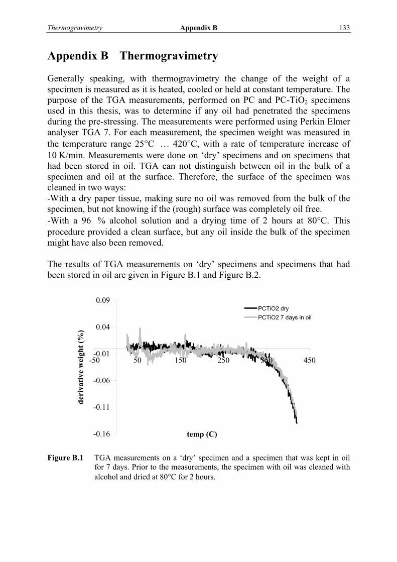
Thermogravimetry Appendix B 133
Appendix B Thermogravimetry
Generally speaking, with thermogravimetry the change of the weight of a specimen is measured as it is heated, cooled or held at constant temperature. The purpose of the TGA measurements, performed on PC and PC-TiO2 specimens used in this thesis, was to determine if any oil had penetrated the specimens during the pre-stressing. The measurements were performed using Perkin Elmer analyser TGA 7. For each measurement, the specimen weight was measured in the temperature range 25°C … 420°C, with a rate of temperature increase of 10 K/min. Measurements were done on ‘dry’ specimens and on specimens that had been stored in oil. TGA can not distinguish between oil in the bulk of a specimen and oil at the surface. Therefore, the surface of the specimen was cleaned in two ways: -With a dry paper tissue, making sure no oil was removed from the bulk of the specimen, but not knowing if the (rough) surface was completely oil free. -With a 96 % alcohol solution and a drying time of 2 hours at 80°C. This procedure provided a clean surface, but any oil inside the bulk of the specimen might have also been removed. The results of TGA measurements on ‘dry’ specimens and specimens that had been stored in oil are given in Figure B.1 and Figure B.2.
-0.16
-0.11
-0.06
-0.01
0.04
0.09
-50 50 150 250 350 450
temp (C)
deri
vativ
e w
eigh
t (%
)
PCTiO2 dryPCTiO2 7 days in oil
Figure B.1 TGA measurements on a ‘dry’ specimen and a specimen that was kept in oil
for 7 days. Prior to the measurements, the specimen with oil was cleaned with alcohol and dried at 80°C for 2 hours.
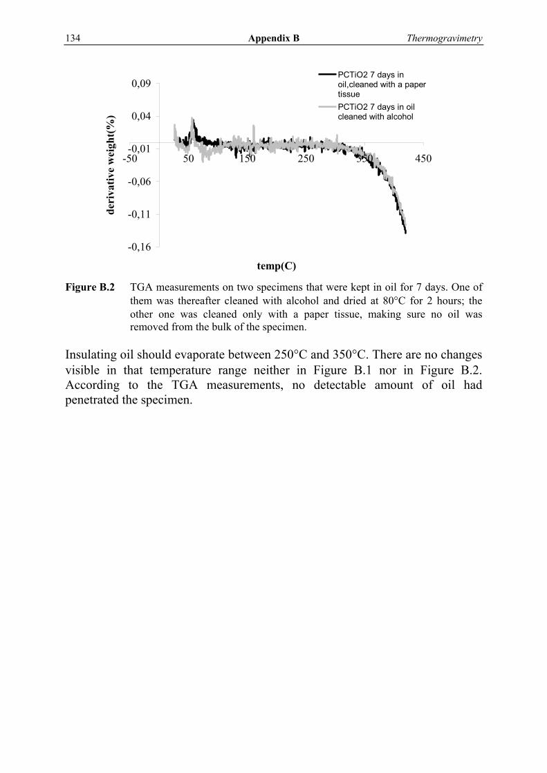
134 Appendix B Thermogravimetry
-0,16
-0,11
-0,06
-0,01
0,04
0,09
-50 50 150 250 350 450
temp(C)
deri
vativ
e w
eigh
t(%
)
PCTiO2 7 days inoil,cleaned with a papertissuePCTiO2 7 days in oilcleaned with alcohol
Figure B.2 TGA measurements on two specimens that were kept in oil for 7 days. One of
them was thereafter cleaned with alcohol and dried at 80°C for 2 hours; the other one was cleaned only with a paper tissue, making sure no oil was removed from the bulk of the specimen.
Insulating oil should evaporate between 250°C and 350°C. There are no changes visible in that temperature range neither in Figure B.1 nor in Figure B.2. According to the TGA measurements, no detectable amount of oil had penetrated the specimen.

Thermogravimetry Appendix B 135

136 Appendix B Thermogravimetry
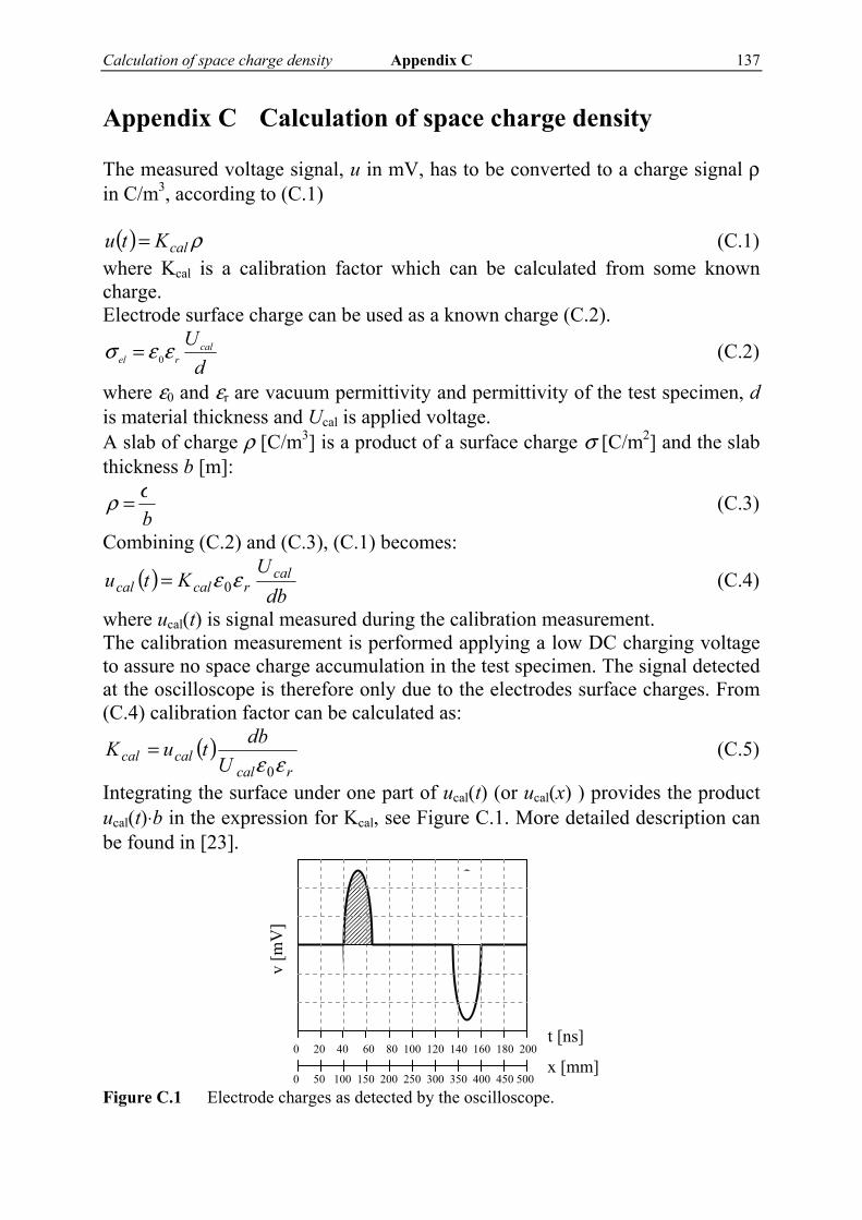
Calculation of space charge density Appendix C 137
Appendix C Calculation of space charge density
The measured voltage signal, u in mV, has to be converted to a charge signal ρ in C/m3, according to (C.1)
( ) ρcalKtu = (C.1) where Kcal is a calibration factor which can be calculated from some known charge. Electrode surface charge can be used as a known charge (C.2).
dUcal
rel εεσ 0= (C.2)
where ε0 and εr are vacuum permittivity and permittivity of the test specimen, d is material thickness and Ucal is applied voltage. A slab of charge ρ [C/m3] is a product of a surface charge σ [C/m2] and the slab thickness b [m]:
bσρ = (C.3)
Combining (C.2) and (C.3), (C.1) becomes:
( )db
UKtu cal
rcalcal εε 0= (C.4)
where ucal(t) is signal measured during the calibration measurement. The calibration measurement is performed applying a low DC charging voltage to assure no space charge accumulation in the test specimen. The signal detected at the oscilloscope is therefore only due to the electrodes surface charges. From (C.4) calibration factor can be calculated as:
( )rcal
calcal UdbtuK
εε 0= (C.5)
Integrating the surface under one part of ucal(t) (or ucal(x) ) provides the product ucal(t)⋅b in the expression for Kcal, see Figure C.1. More detailed description can be found in [23]. Figure C.1 Electrode charges as detected by the oscilloscope.
v [m
V]
t [ns] 0 20 40 60 80 100 120 140 160 180 200
0 50 100 150 200 250 300 350 400 450 500 x [mm]

138 Appendix C Calculation of space charge density

Charge accumulation Appendix D 139
Appendix D Charge accumulation
In an electro-quasi-static field, Maxwell’s equations can be written as:
0=×∇→
E (D.1)
ρε =⋅∇=⋅∇→→
ED (D.2)
0=∂∂+⋅∇
→
tρJ (D.3)
where →
D is the flux density, →
E is the electric field strength, →
J is the current density, ε is the dielectric permittivity and ρ is the free space charge density. →
J obeys Ohm’s law: →→
= EJ σ (D.4) where σ is the conductivity of the material.
Replacing →
J and ρ in (D.3), with →
Eσ respectively→
⋅∇ Eε , results in:
0=∇+∇→
→
EdtdE εσ (D.5)
Figure D.1 Interface between two dielectrics. Applied voltage is a step function with u = 0
for t ≤ 0 and u = U for t > 0.
In a homogeneous electrical field, assuming →
E ≠ 0 in one direction, Figure D.1, (D.5) becomes [13]:
( ) ( ) 0=−+− BBAABBAA EEdtdEE εεσσ (D.6)
where σA and σB denote the conductivity, εA and εB denote the permittivity, and EA and Eb denote the electrical field strengths in materials A and B. Applying dAEA + dBEB = U, and eliminating EB, the solution of the differential equation (D.6) can be written as:
dA dB
u+ u-
σAεA σBεB
EA EB t
U
140 Appendix D Charge accumulation
( ) ττ
εεε
σσσ t
BAAB
Bt
BAAB
BA e
ddUe
ddUE −−
++−
+= 1 (D.7)
Where dA and dB are material thicknesses and τ is the time constant. Denoting the charge accumulated at the interface of the two dielectrics shown in Figure D.1, with κ, the equation (D.2) can be written as:
κεε =− BBAA EE (D.8) Applying dAEA + dBEB = U to eliminate EB from (D.8), and filling in obtained expression for EA from (D.7), the charge accumulated at the interface can be written as:
( )τ
σσεσεσκ
t
BAAB
BAAB eUdd
−−⋅⋅+−= 1 (D.9)

Charge accumulation Appendix D 141

142 Appendix D Charge accumulation
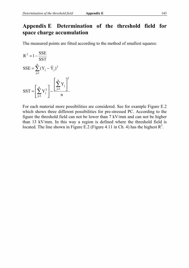
Determination of the threshold field Appendix E 143
Appendix E Determination of the threshold field for space charge accumulation
The measured points are fitted according to the method of smallest squares:
n
YYSST
)YY(SSE
SSTSSE1R
2n
1jjn
1j
2j
2j
n
1jj
2
⎥⎦
⎤⎢⎣
⎡
−⎥⎦
⎤⎢⎣
⎡=
−=
−=
∑∑
∑
=
=
=
For each material more possibilities are considered. See for example Figure E.2 which shows three different possibilities for pre-stressed PC. According to the figure the threshold field can not be lower than 7 kV/mm and can not be higher than 13 kV/mm. In this way a region is defined where the threshold field is located. The line shown in Figure E.2 (Figure 4.11 in Ch. 4) has the highest R2.

144 Appendix E Determination of the threshold field
Determination of the threshold field for space charge accumulation in PC The final results as shown in Ch 4, are presented in Figure E.1 and Figure E.2. Figure E.3 shows possible trend lines.
Figure E.1 Determination of the threshold field for space charge accumulation in virgin
PC
Figure E.2 Determination of the threshold field for space charge accumulation in pre-
stressed PC. The threshold field is located in the indicated electric field range.
0.01
0.1
1
10 ch
arge
den
sity
[ μC
/cm
3 ]
applied field [kV/mm]
new PC
1 10 100 2 3 4 5 20 30 40 50
Eth,sc
detection limit
y= 0.0026(x1.69)R2= 0.99
pre-stressed PC
0.01
0.1
1
10
char
ge d
ensi
ty [ μ
C/c
m3 ]
applied field [kV/mm]1 10 100 2 3 4 5 20 30 40 50
detection limit
13 7

Determination of the threshold field Appendix E 145
Figure E.3 Different possibilities for the threshold field for space charge accumulation in
pre-stressed PC. Line 1 and line 3 define the highest and the lowest possible threshold field.
pre-stressed PC
0.01
0.1
1
10
char
ge d
ensi
ty [ μ
C/c
m3 ]
applied field [kV/mm]1 10 100 2 3 4 5 20 30 40 50
detection limit
1 y= 0.0004(x2.73)R2= 0.907
pre-stressed PC
0.01
0.1
1
10
char
ge d
ensi
ty [ μ
C/c
m3 ]
applied field [kV/mm]1 10 100 2 3 4 5 20 30 40 50
detection limit
2 y= 0.0011(x 1.85)R2=0.948
pre-stressed PC
0.01
0.1
1
10
char
ge d
ensi
ty [ μ
C/c
m3 ]
applied field [kV/mm]1 10 100 2 3 4 5 20 30 40 50
detection limit
3 y= 0.0037(x1.48)R2= 0.936

146 Appendix E Determination of the threshold field
Determination of the threshold field for space charge accumulation in PC-TiO2 The final results as shown in Ch 4, are presented in Figure E.4 and Figure E.5. Figure E.6 and Figure E.7 show possible trend lines for threshold determination of virgin and pre-stressed PC-TiO2.
Figure E.4 Determination of the threshold field for space charge accumulation in virgin
PC-TiO2. The threshold field is located in the indicated electric field range. See also Figure E.6
Figure E.5 Determination of the threshold field for space charge accumulation in pre-
stressed PC-TiO2. The threshold field is located in the indicated electric field range. See also Figure E.7
E [kV/mm]
0.01
0.1
1
10
char
ge d
ensit
y [μ
C/c
m3 ]
pre-stressed PCTiO2
1 10 100 2 3 4 5 20 30 40 50
detection limit
2
y= 0.0183(x0.92)R2= 0.943
2.8 5.8
new PCTiO2
0.01
0.1
1
10
char
ge d
ensi
ty [ μ
C/c
m3 ]
E [kV/mm]1 10 100 2 3 4 5 20 30 40 50
detection limit
3.3 4.7
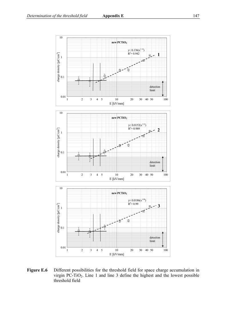
Determination of the threshold field Appendix E 147
Figure E.6 Different possibilities for the threshold field for space charge accumulation in
virgin PC-TiO2. Line 1 and line 3 define the highest and the lowest possible threshold field
new PCTiO2
0.01
0.1
1
10
char
ge d
ensi
ty [ μ
C/c
m3 ]
E [kV/mm]1 10 100 2 3 4 5 20 30 40 50
detection limit
1y= 0.136(x1.12)R2= 0.942
new PCTiO2
0.01
0.1
1
10
char
ge d
ensi
ty [ μ
C/c
m3 ]
E [kV/mm]1 10 100 2 3 4 5 20 30 40 50
detection limit
2y= 0.0152(x1.12) R2= 0.989
new PCTiO2
0.01
0.1
1
10
char
ge d
ensi
ty [ μ
C/c
m3 ]
E [kV/mm]1 10 100 2 3 4 5 20 30 40 50
detection limit
3 y= 0.0186(x1.06) R2= 0.99
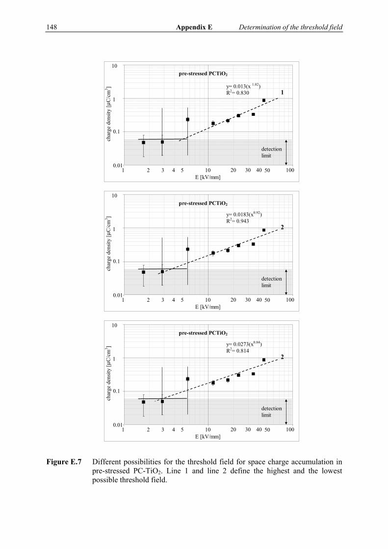
148 Appendix E Determination of the threshold field
Figure E.7 Different possibilities for the threshold field for space charge accumulation in
pre-stressed PC-TiO2. Line 1 and line 2 define the highest and the lowest possible threshold field.
E [kV/mm]
0.01
0.1
1
10
char
ge d
ensit
y [μ
C/c
m3 ]
pre-stressed PCTiO2
1 10 100 2 3 4 5 20 30 40 50
detection limit
1 y= 0.013(x 1.02)R2= 0.830
E [kV/mm]
0.01
0.1
1
10
char
ge d
ensit
y [μ
C/c
m3 ]
pre-stressed PCTiO2
1 10 100 2 3 4 5 20 30 40 50
detection limit
2
y= 0.0183(x0.92)R2= 0.943
E [kV/mm]
0.01
0.1
1
10
char
ge d
ensit
y [μ
C/c
m3 ]
pre-stressed PCTiO2
1 10 100 2 3 4 5 20 30 40 50
detection limit
2
y= 0.0273(x0.84)R2= 0.814

Determination of the threshold field Appendix E 149

150 Appendix E Determination of the threshold field

Polarization current fit Appendix F 151
Appendix F Polarization current fit
The measured polarization currents can be described by the following additive expression1
ctataI nn ++= −− 2121 (F.1)
Where a1, a2, n1, n2 and c are constants and t is the time. When t approaches infinity only the constant c will remain. Therefore, the constant c is actually the steady-state value of the polarization current, the conduction current.
1 The purpose of the used expression is to give the best fit: the physical meaning, if any, is not considered.

152 Appendix F Polarization current fit
PC virgin and pre-stresse: polarization current measurements and fits Polarization currents measured in virgin PC specimens and fits according to expression (1) are shown in Figure F.1. Results of the measurements and fits for pre-stressed PC are given in Figure F.2 Figure F.1 Polarization current measurements and fits of virgin P
1,E-15
1,E-14
1,E-13
1,E-12
1,E-11
1,E-10
1,E-09
1,E-08
1,E-07
1,E-06
1,E+01 1,E+02 1,E+03 1,E+04 1,E+05 1,E+06 1,E+07
Polarization time [sec]
Pola
rizat
ion
curr
ent [
A]
2.9 kV/mm, fit2,9 kV/mm, measurement
1,E-15
1,E-14
1,E-13
1,E-12
1,E-11
1,E-10
1,E-09
1,E-08
1,E-07
1,E-06
1,E+01 1,E+02 1,E+03 1,E+04 1,E+05 1,E+06 1,E+07
Polarization time [sec]Po
lariz
atio
n cu
rren
t [A
]
5.7 kV/mm, fit
5.7 kV/mm, measurement
1,E-15
1,E-14
1,E-13
1,E-12
1,E-11
1,E-10
1,E-09
1,E-08
1,E-07
1,E-06
1,E+01 1,E+02 1,E+03 1,E+04 1,E+05 1,E+06 1,E+07
Polarization time [sec]
Pola
rizat
ion
curr
ent [
A]
11.4 kV/mm, fit
11.4 kV/mm, measurement
1,E-15
1,E-14
1,E-13
1,E-12
1,E-11
1,E-10
1,E-09
1,E-08
1,E-07
1,E-06
1,E+01 1,E+02 1,E+03 1,E+04 1,E+05 1,E+06 1,E+07
Polarization time [sec]
Pola
rizat
ion
curr
ent [
A]
17.1 kV/mm, fit
17.1 kV/mm, measurement
1,E-15
1,E-14
1,E-13
1,E-12
1,E-11
1,E-10
1,E-09
1,E-08
1,E-07
1,E-06
1,E+01 1,E+02 1,E+03 1,E+04 1,E+05 1,E+06 1,E+07
Polarization time [sec]
Pola
rizat
ion
curr
ent [
A]
22.9 kV/mm, fit
22.9 kV/mm, measurement
1,E-15
1,E-14
1,E-13
1,E-12
1,E-11
1,E-10
1,E-09
1,E-08
1,E-07
1,E-06
1,E+01 1,E+02 1,E+03 1,E+04 1,E+05 1,E+06 1,E+07
Polarization time [sec]
Pola
rizat
ion
curr
ent [
A]
34.3 kV/mm, fit
34.3 kV/mm, measurement

Polarization current fit Appendix F 153
Figure F.2 Polarization current measurements and fits of pre-stressed PC
1,E-15
1,E-14
1,E-13
1,E-12
1,E-11
1,E-10
1,E-09
1,E-08
1,E-07
1,E-06
1,E+01 1,E+02 1,E+03 1,E+04 1,E+05 1,E+06 1,E+07
Polarization time [sec]
Pola
rizat
ion
curr
ent [
A]
2.9 kV/mm, fit
2.9 kV/mm, measurement
1,E-15
1,E-14
1,E-13
1,E-12
1,E-11
1,E-10
1,E-09
1,E-08
1,E-07
1,E-06
1,E+01 1,E+02 1,E+03 1,E+04 1,E+05 1,E+06 1,E+07
Polarization time [sec]
Pola
rizat
ion
curr
ent [
A]
5.7 kV/mm, fit
5.7 kV/mm, measurement
1,E-15
1,E-14
1,E-13
1,E-12
1,E-11
1,E-10
1,E-09
1,E-08
1,E-07
1,E-06
1,E+01 1,E+02 1,E+03 1,E+04 1,E+05 1,E+06 1,E+07
Polarization time [sec]
Pola
rizat
ion
curr
ent [
A]
11.4 kV/mm, fit
11.4 kV/mm, measurement
1,E-15
1,E-14
1,E-13
1,E-12
1,E-11
1,E-10
1,E-09
1,E-08
1,E-07
1,E-06
1,E+01 1,E+02 1,E+03 1,E+04 1,E+05 1,E+06 1,E+07
Poalrization time [sec]
Poal
rizat
ion
curr
ent [
A]
17.1 kV/mm, fit
17.1 kV/mm, measurement
1,E-15
1,E-14
1,E-13
1,E-12
1,E-11
1,E-10
1,E-09
1,E-08
1,E-07
1,E-06
1,E+01 1,E+02 1,E+03 1,E+04 1,E+05 1,E+06 1,E+07
Polarization time [sec]
Pola
rizat
ion
curr
ent [
A]
22.9 kV/mm, fit
22.9 kV/mm, measurement
1,E-15
1,E-14
1,E-13
1,E-12
1,E-11
1,E-10
1,E-09
1,E-08
1,E-07
1,E-06
1,E+01 1,E+02 1,E+03 1,E+04 1,E+05 1,E+06 1,E+07
Poalrization time [sec]
Pola
rizat
ion
curr
ent [
A]
34.3 kV/mm, fit
34.3 kV/mm, measurement
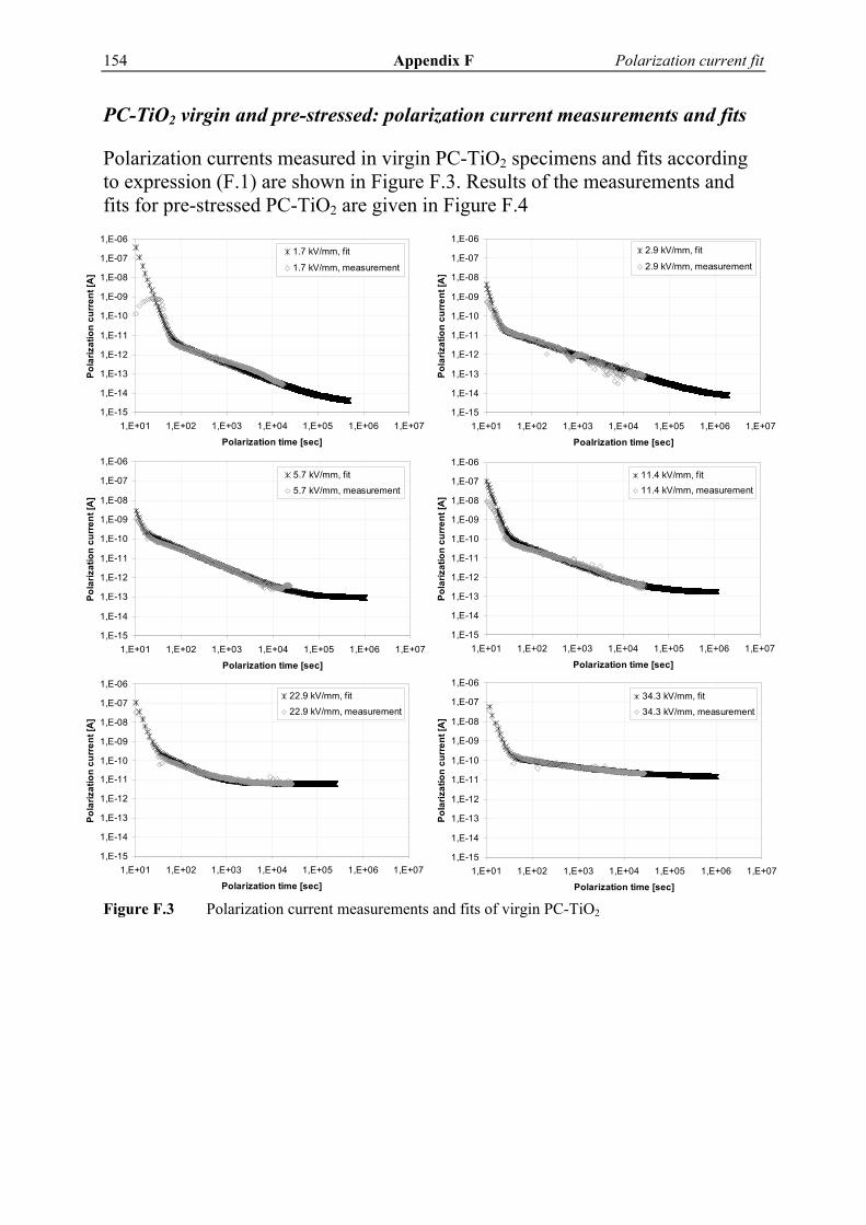
154 Appendix F Polarization current fit
PC-TiO2 virgin and pre-stressed: polarization current measurements and fits Polarization currents measured in virgin PC-TiO2 specimens and fits according to expression (F.1) are shown in Figure F.3. Results of the measurements and fits for pre-stressed PC-TiO2 are given in Figure F.4 Figure F.3 Polarization current measurements and fits of virgin PC-TiO2
1,E-15
1,E-14
1,E-13
1,E-12
1,E-11
1,E-10
1,E-09
1,E-08
1,E-07
1,E-06
1,E+01 1,E+02 1,E+03 1,E+04 1,E+05 1,E+06 1,E+07
Polarization time [sec]
Pola
rizat
ion
curr
ent [
A]
1.7 kV/mm, fit
1.7 kV/mm, measurement
1,E-15
1,E-14
1,E-13
1,E-12
1,E-11
1,E-10
1,E-09
1,E-08
1,E-07
1,E-06
1,E+01 1,E+02 1,E+03 1,E+04 1,E+05 1,E+06 1,E+07
Poalrization time [sec]Po
lariz
atio
n cu
rren
t [A
]
2.9 kV/mm, fit
2.9 kV/mm, measurement
1,E-15
1,E-14
1,E-13
1,E-12
1,E-11
1,E-10
1,E-09
1,E-08
1,E-07
1,E-06
1,E+01 1,E+02 1,E+03 1,E+04 1,E+05 1,E+06 1,E+07
Polarization time [sec]
Pola
rizat
ion
curr
ent [
A]
5.7 kV/mm, fit
5.7 kV/mm, measurement
1,E-15
1,E-14
1,E-13
1,E-12
1,E-11
1,E-10
1,E-09
1,E-08
1,E-07
1,E-06
1,E+01 1,E+02 1,E+03 1,E+04 1,E+05 1,E+06 1,E+07
Polarization time [sec]
Pola
rizat
ion
curr
ent [
A]
11.4 kV/mm, fit11.4 kV/mm, measurement
1,E-15
1,E-14
1,E-13
1,E-12
1,E-11
1,E-10
1,E-09
1,E-08
1,E-07
1,E-06
1,E+01 1,E+02 1,E+03 1,E+04 1,E+05 1,E+06 1,E+07
Polarization time [sec]
Pola
rizat
ion
curr
ent [
A]
22.9 kV/mm, fit
22.9 kV/mm, measurement
1,E-15
1,E-14
1,E-13
1,E-12
1,E-11
1,E-10
1,E-09
1,E-08
1,E-07
1,E-06
1,E+01 1,E+02 1,E+03 1,E+04 1,E+05 1,E+06 1,E+07
Polarization time [sec]
Pola
rizat
ion
curr
ent [
A]
34.3 kV/mm, fit
34.3 kV/mm, measurement

Polarization current fit Appendix F 155
Figure F.4 Polarization current measurements and fits of pre-stressed PC-TiO2
1,E-15
1,E-14
1,E-13
1,E-12
1,E-11
1,E-10
1,E-09
1,E-08
1,E-07
1,E-06
1,E+01 1,E+02 1,E+03 1,E+04 1,E+05 1,E+06 1,E+07
Polarization time [sec]
Pola
rizat
ion
curr
ent [
A]
1.7 kV/mm, fit
1.7 kV/mm, measurement
1,E-15
1,E-14
1,E-13
1,E-12
1,E-11
1,E-10
1,E-09
1,E-08
1,E-07
1,E-06
1,E+01 1,E+02 1,E+03 1,E+04 1,E+05 1,E+06 1,E+07
Polarization time [sec]
Pola
rizat
ion
curr
ent [
A]
2.9 kV/mm, fit
2.9 kV/mm, measurement
1,E-15
1,E-14
1,E-13
1,E-12
1,E-11
1,E-10
1,E-09
1,E-08
1,E-07
1,E-06
1,E+01 1,E+02 1,E+03 1,E+04 1,E+05 1,E+06 1,E+07
Polarization time [sec]
Pola
rizat
ion
curr
ent [
A]
5.7 kV/mm, fit5.7 kV/mm, measurement
1,E-15
1,E-14
1,E-13
1,E-12
1,E-11
1,E-10
1,E-09
1,E-08
1,E-07
1,E-06
1,E+01 1,E+02 1,E+03 1,E+04 1,E+05 1,E+06 1,E+07
Polarization time [sec]
Pola
rizat
ion
curr
ent [
A]
11.4 kV/mm, fit
11.4 kV/mm, measurement
1,E-15
1,E-14
1,E-13
1,E-12
1,E-11
1,E-10
1,E-09
1,E-08
1,E-07
1,E-06
1,E+01 1,E+02 1,E+03 1,E+04 1,E+05 1,E+06 1,E+07
Polarization time [sec]
Pola
rizat
ion
curr
ent [
A]
17.1 kV/mm, fit17.1 kV/mm, measurement
1,E-15
1,E-14
1,E-13
1,E-12
1,E-11
1,E-10
1,E-09
1,E-08
1,E-07
1,E-06
1,E+01 1,E+02 1,E+03 1,E+04 1,E+05 1,E+06 1,E+07
Polarization time [sec]
Pola
rizat
ion
curr
ent [
A]
22.9 kV/mm, fit
22.9 kV/mm, measurement
1,E-15
1,E-14
1,E-13
1,E-12
1,E-11
1,E-10
1,E-09
1,E-08
1,E-07
1,E-06
1,E+01 1,E+02 1,E+03 1,E+04 1,E+05 1,E+06 1,E+07
Polarization time [sec]
Pol
ariz
atio
n cu
rren
t [A
]
34.3 kV/mm, fit
34.3 kV/mm, measurement

156 Appendix F Polarization current fit

157 Appendix G Polarization current
Appendix G Polarization current
A dielectric material contains hardly any free charge carriers. Almost all charge carriers are bounded in the material. An externally applied electric field can influence these charge carriers in a way that a displacement of positive charge carriers take place with respect to negative charge carriers. A well known phenomenon called polarization P(t). The polarization P(t) and a (pulse) excitation E(t) are related through the dielectric response function f(t).
( ) ( ) ( )tftEεtP Δ= 0 (G.1) Thereby fulfills the dielectric response function the following conditions: Causality: ( ) 0≡tf for t < 0; The material possesses no permanent polarization: ( ) 0=
∞→tflim
t
Assuming linearity of the dielectric material, the superposition principle can be applied: the electrical polarization P(t) caused by a series of n pulse excitations can be described as a sum of n polarizations P(t1) …P(tn), each of them being caused by a E-pulse.
( ) ( ) ( ) ( )[ ]nn ttfE...ttfEttfEttP −++−+−Δ= 22110ε (G.2) With the number of excitation pulses approaching infinity, the total polarization obtains the form of a convolution integral:
( ) ( ) ( ) τττε dtEftP −= ∫∞
00 (G.3)
The physical interpretation of the convolution integral is that the system retains memory of pat excitation. In case of a step excitation given with:
( ) 0=tE for t<0 ( ) 0EtE = for t>0
The integral given in (G.3) becomes:

158 Appendix G Polarization current
( ) ( ) ττε dfEtPt
∫=0
00 (G.4)
Using the Ampere’s law and the formula for dielectric displacement D(t), the total current density can be written as given in expression (G.5):
( ) ( ) ( )321
321
currentnpolarizati
esargchfreecurrentDC
ttDtEHtJ
∂∂+=×∇= σ
( ) ( ) ( ) ( ) ⎥⎦
⎤⎢⎣
⎡+=+= ∫
t
dftEtPtE)t(D0
000 1 ττεε
( ) ( ) ( ) ( ) ( )[ ]tftEEdftEt
EtJt
++=⎥⎦
⎤⎢⎣
⎡+
∂∂+= ∫ δεσττεσ 000
0000 1 (G.5)
For an object with a geometrical capacity C0 and applied step voltage U0 for a certain time t1, the total polarization current through the object can be written as:
( ) ( ) ( )⎥⎦
⎤⎢⎣
⎡++= tftCUtI P δ
εσ
000 0 < t < t1 (G.6)
The current after the U0 is switched off, the depolarization current is:
( ) ( )tfCUtI D 00= t > t1 (G.7) Figure G.1 Polarization and depolarization current
I(t)
t1
Polarization current
Depolarization current
t

159 Appendix G Polarization current

160 Appendix G Polarization current

References 161
References
[1] R. Bartnikas, Engineering Dielectrics, Volume IIB, Electrical Properties
of Solid Insulating Materials: Measurements Techniques, ISBN 0-8031-0491-x, pp. 3, 1987.
[2] A. Cerifi, M.A. Dakka, A. Toureille, The validation of the thermal step
method, IEEE Transactions on Dielectrics and Electrical Insulation, Vol. 27, No. 6, pp. 1152 – 1158, 1992.
[3] C. Alquié, G. Dreyfuss, J. Lewiner, Stress-wave probing of electric field
distributions in dielectrics, Phys. Rev. Lett., Vol. 47, No. 20, pp. 1483 –1487, 1981.
[4] G.M. Sessler, J.E. West, G. Gerhard, High resolution laser-pulse method
for measuring charge distribution in dielectrics, Phys. Rev. Lett., Vol. 48, No. 8, pp. 563 – 566, 1982.
[5] T. Takada, Y. Tanaka, N. Adachi, X. Qin, Comparison between the PEA
method and the PWP method for space charge measurements in solid dielectrics, IEEE Transactions on Dielectrics and Electrical Insulation, Vol. 5, No. 6, pp. 944 – 950, 1998.
[6] W. Eisenmenger, M. Haardt, Observation of charge compensated
polarization zones in PVDF films by piezoelectric acoustic step-wave response, Solid State Community, Vol. 41, No. 12, pp. 917 – 920, 1982.
[7] Y. Li, M. Yasuda, T. Takada, Pulsed electroacoustic method for
measurement of charge accumulation in solid dielectrics, IEEE Transactions on Dielectrics and Electrical Insulation, Vol. 1, No. 2, pp. 188 – 195, 1994.
[8] T. Maeno, H. Kushibe, T. Takada, C.M. Cooke, Pulsed electro-acoustic
method for the measurements of volume charge in e-beam irradiated PMMA, IEEE Conference on electrical Insulation and Dielectric Phenomena, proceedings, pp. 389 – 397, 1985.
[9] T. Maeno, T. Futami, H. Kushibe, T. Takada, C.M. Cooke, Measurement
of spatial charge distribution in thick dielectrics using pulsed

162 References
electroacoustic method, IEEE Transactions on Dielectrics and Electrical Insulation, Vol. 23, No. 3, pp. 433 – 439, 1988.
[10] T. Takada, Acoustic and Optical Methods for Measuring Electric Charge
Distributions in Dielectrics, IEEE Transaction on DEI, Vol. 6, No.5, pp 519 – 574, 1999.
[11] K. Fukunaga, Innovative PEA space charge measurement system for
industrial applications, IEEE Electrical Insulation Magazine, Vol. 20, No. 2, pp. 18 – 26, 2004.
[12] J.M. Alison, The pulsed electro-acoustic method for the measurement of
the dynamic space charge profile within insulators, in Space charge in solid dielectric, edit by J.C. Fothergill and L.A .Dissado, ISBN 0-9533538-0-X, pp. 93 – 121, 1998.
[13] F.H. Kreuger, Industrial High DC Voltage, Volume III, Delft University
Press, ISBN 90-407-1110-0, 1995. [14] T. Mizutani, Space Charge Measurement Techniques and Space Charge
in Polyethylene, IEEE Transactions on Dielectrics and Electrical Insulation, Vol. 1, No. 5, pp 923 – 933, 1994.
[15] R. Bodega, Space Charge Accumulation in Polymeric High Voltage DC
Cable Systems, PhD thesis TU Delft, ISBN 90-8559-228-3, 2006. [16] J.C. Fothergill, G.C. Montanari, G.C. Stevens, C. Laurent, G. Teyssedre,
U.H. Nilsson, G. Platbrood, Electrical, Microstructural, Physical and Chemical Characterization of HV XLPE Cable Peelings for an Electrical Aging Diagnostic Data Base, IEEE Transaction on Dielectrics and Electrical Insulation, Vol. 10, No. 3, pp 514 – 527, 2003.
[17] M. Salah Khalil, International Research and Development Trends and
Problems of HVDC Cables with Polymeric Insulation, IEEE Electrical Insulation Magazine, Vol. 13, No. 6, pp 35 – 47, 1997.
[18] T. Mizutani, Y. Taniguchi, T. Hori, M. Ishioka, Space Charge Dynamics
of Low-density Polyethylene, 2002 Annual Report Conference on Electrical Insulation and Dielectric Phenomena, pp. 618 – 621, 2002.
[19] E. Ildstad, F. Mauseth, G. Balog, Space Charge and Electric Field
Distribution in Current Loaded Polyethylene Insulated HVDC Cables, XIIIth International Symposium on High Voltage Engineering, Netherlands 2003, pp. 1 – 5, 2003.
References 163
[20] J. Ho Nam, K.S. Suh, Interfacial Charge of XLPE/EPDM Laminates, Proceedings of 1998 International Symposium on Electrical Insulating Materials, pp. 187 – 189, 1998.
[21] O. Gallot-Lavallée, G. Teyssedre, C. Laurent, S. Rowe, Space Charge and
Orientational Polarization within Epoxy as Probed by the Pulsed Electro-Acoustic Technique, 2003 Annual Conference on Electrical Insulation and Dielectric Phenomena, pp. 249 – 252, 2003.
[22] K. Fukanaga, T. Maeno, V. Grisseri, Space Charge Observation of a
Filler Free Epoxy Resin, 2000 Conference on Electrical Insulation and Dielectric Phenomena, pp. 125 – 127, 2000.
[23] M.J.P. Jeroense, Charges and Discharges in HVDC cables, PhD thesis TU
Delft, Delft University Press, 1997. [24] J. Beyer, Space Charge and Partial Discharge Phenomena in HVDC
Devices, PhD thesis TU Delft, Delft University Press, 2001. [25] N. Vella, A. El Ila Joumha, A. Toureille, Space charge measurements by
the thermal step method and TSDC in PMMA, IEEE transactions on DEI, Vol. 4, pp. 230 – 235, 1994.
[26] G.C. Montanari, G. Mazzanti, L.A. Dissado, D.K. Das-Gupta, Space
Charge as a Trigger for Electrical Ageing of Polymeric Insulation, Charges in Solid Dielectrics, The Dielectric Society Ed, UK, pp 259 – 272, 1998.
[27] L.A. Dissado, G. Mazzanti, G.C. Montanari, The Role of Trapped Space
Charge in the Electrical Ageing of Insulating Materials, IEEE transactions on DEI, Vol. 4, pp 496 – 506, 1997.
[28] G.C. Montanari, D. Fabiani, Evaluation of DC Insulation Performance
Based on Space Charge Measurements and Accelerated Life Tests, IEEE Transactions on Dielectrics and Electrical Insulation, Vol. 7, pp. 322 – 328, 2000.
[29] G. Mazzanti, G.C. Montanari, F. Palmieri, Quantities Extracted from
Space Charge Measurements as Markers for Insulation Ageing, IEEE Transactions on Dielectrics and Electrical Insulation, Vol. 10, 2003.
[30] L. Simoni, G. Mazzanti, G.C. Montanari, L.Lefebre, A General Multi –
stress Life Model for Insulating Materials with or without Evidence for
164 References
Thresholds, IEEE Transactions on Dielectrics and Electrical Insulation, Vol.28, pp. 349 – 364, 1993.
[31] J-P. Crine, A Molecular Model to Evaluate the Impact of Aging on Space
Charges in Polymer Dielectrics, IEEE Transactions on Dielectrics and Electrical Insulation, Vol.4, pp. 487 – 495, 1997.
[32] G. Mazzanti, G.C. Montanari, L. Simoni, Considerations on the
Compatibility Conditions of the Eyring Model Applied for Multiple Stresses, IEEE Transactions on Dielectrics and Electrical Insulation, pp. 771 – 776, 1993.
[33] J-L. Parpal, J-P. Crine, C. Dang, Electrical Aging of Extruded Cables: A
Physical Model, IEEE Transactions on Dielectrics and Electrical Insulation, Vol.4, pp. 197 – 209, 1997.
[34] J-P. Crine, Influence of High DC Electrical Fields on Some Aging
Properties of XLPE, Conference Record of the 2000 IEEE Symposium on Electrical Insulation, Anaheim, CA USA, pp. 101 – 104, 2000.
[35] L.A Dissado, G. Mazzanti, G.C. Montanari, The Role of Trapped Space
Charge in the Electrical Aging of Insulating Materials, IEEE Transactions on Dielectrics and Electrical Insulation, Vol.4, pp. 496 – 506, 1997.
[36] L.A. Dissado, G. Mazzanti, G.C. Montanari, The Incorporation of Space
Charge Degradation in the Life Model for Electrical Insulating Materials, IEEE Transactions on Dielectrics and Electrical Insulation, Vol.2, pp. 1147 – 1158, 1995.
[37] G.C. Montanari, Simoni L., Aging Phenomenology and Modeling, IEEE
Transactions on Dielectrics and Electrical Insulation, Vol.28, pp. 755 – 776, 1993.
[38] G.C. Montanari, Extraction of Information from Space Charge
Measurements and Correlation with Insulation Ageing, Conference Record of the 4th International Conference on Electric Charges and Non-conductive Materials, pp. 178 – 184, 2001.
[39] L.A Dissado, G. Mazzanti, G. C. Montanari, A New Thermo-Electrical
Life Model Based on Space Charge Trapping, Conference Record of the 1996 IEEE International Symposium on Electrical insulation, pp. 642-645, 1996.

References 165
[40] R. Bartnikas, Engineering Dielectrics, Volume IIA, Electrical Properties of Solid Insulating Materials: Molecular structure and Electrical Behaviour, 1987.
[41] L.A. Dissado, J.C. Fothergill, Electrical Degradation and Breakdown in
Polymers, ISBN 0 86341 196 7, 1992. [42] J. Tao, Surface charge accumulation in SF6, PhD thesis TU Delft, 1993. [43] W.D. Callister, Materials Science and Engineering: an Introduction, ISBN
0-471-32013-7, 1999. [44] B. Alijagic-Jonuz, Lifetime performance of non-energy HVDC insulation
systems, Triumvirate III report 3, TU Delft, 2002. [45] G. Schaumburg, New Broadband Dielectric Spectrometers, Scientific
Newsletter for dielectric spectroscopy, Issue July 1994. [46] Alpha-A High Resolution Dielectric, Conductivity, Impedance Modular
Measurement System: Users Manual, Rev. 2.00 by AIS Analytical Systems GmbH, Issue 2003.
[47] P.H.F. Morshuis, Lecture Notes:High voltage DC, Delft University of
Technology, Delft, The Netherlands, 2006. [48] J. C. Maxwell, A Treatise on Electricity and Magnetism, Vol. 1, 2nd
edition, Clarendon Press, Oxford, England, 1881. [49] K.W. Wagner, Erklärung der dielektrischen Nachwirkungsvorgänge auf
Grund Maxwellscher Vorstellungen, Archiev f. Elektrotechnik, No.2, pp. 371 – 378, 1914.
[50] J.C. Fothergill, Trap Limited Conduction, Lecture notes [51] ref in [52], B. Alijagic-Jonuz, P.H.F. Morshuis, J.J. Smit, Changing of
Space Charge Related Material Properties Due to Electrical Aging, The 7th International Conference on Properties and Applications of Dielectric Materials, pp. 1 – 5, Nagoya, Japan, June 2003.
[52] B. Alijagic-Jonuz, P.H.F. Morshuis, J.J. Smit, Changing of Space Charge
Related Material Properties Due to Electrical Aging, The 7th International Conference on Properties and Applications of Dielectric Materials, pp. 1 – 5, Nagoya, Japan, June 2003.

166 References
[53] B. Holmgren, Dielectric response, breakdown strength and water tree
content of medium voltage XLPE cables, PhD thesis, KTH Höskoletryckeriet, Stockholm, Sweden, 1997.
[54] B. Alijagic-Jonuz , Bepalen van toestand van midenspanningskabels door
middel van RVM metingen, Master thesis, TU Delft, 2000. [55] H.A. Haus, J.R. Melchers, Electromagnetic Fields and Energy, Prentice
Hall, Inc., Englewood Cliffs, New Yersey, 2002. [56] B. Alijagic-Jonuz, P.H.F. Morshuis, J.J. Smit, Broadband dielectric
spectroscopy on different new and aged polymeric materials Annual report conference on electrical insulation and dielectric phenomena, pp .275 – 278, CEIDP 2004.
[57] M. Wubbenhorst, J. van Turnhout, Lecture Notes: Dielectric Properties of
Polymers, Delft University of Technology, The Netherlands, 2002. [58] L.A. Dissado, Physics of Space Charge, HVDC WP3 Report [59] L.A. Dissado, C. Laurent, G.C. Montanari, P.H.F. Morshuis,
Demonstrating a Threshold for Trapped Space Charge Accumulation in Solid Dielectrics under DC Field, IEEE Transactions on Dielectrics and Electrical Insulation, Vol. 12, No. 3, pp. 612 – 620, June 2005.
[60] T.J. Lewis, Ed J.C. Fothergill and L.A. Dissado, The micro-physics of
charge in solid dielectrics, in Space charge in solid dielectrics, The dielectric society, London, pp. 1 – 17, 1998.
[61] P. Frübing, D. Blischke, R. Gerhard-Multhaupt, B. Tiersch, M. Salah
Khalil, Dielectric relaxations in titanium-dioxide-filled polyethylene: Filler-induced chemical modifications provide the dielectric response, Annual Report Conference on Electrical Insulation and Dielectric Phenomena, 2001.
[62] B. Alijagic-Jonuz, Lifetime performance of non-energy HVDC insulation
systems, Triumvirate III report 2, TU Delft, 2002. [63] T. John Lewin, Workshop on Fundamental aspects of Insulation Aging
Mechanisms
References 167
[64] M. Wubbenhorst, J. van Turnhout, Conduction-Free Dielectric Loss ∂ε/∂lnf – a Powerful Tool for the Analysis of Strong (Ion) Conducting Dielectric Materials, Dielectric Newsletter, Scientific newsletter for dielectric spectroscopy, Issue November 2000.

168 References

List of publications 169
List of publications
B. Alijagic-Jonuz, P.H.F. Morshuis, J. Pellis, H.J. van Breen , J.J. Smit Detection of water trees in medium voltage XLPE cables by return voltage measurements, IEEE Annual report, Volume II, 2000. B. Alijagic-Jonuz, P.H.F. Morshuis, J.J. Smit, J. Pellis, Detection of thermal ageing of mass impregnated medium voltage cables by recovery voltage measurements, Proceedings, Societe Françoise du Vide, pp. 491 – 494, Paris, 2001.
B. Alijagic-Jonuz, P.H.F. Morshuis, J.J. Smit, Influence of Insulating Oil on Space Charge Formation and Electrical Threshold in Polycarbonate with Inorganic Filler, IEEE Conference on electrical insulation, proceedings, pp. 302 – 305, 2002. B. Alijagic-Jonuz, P.H.F. Morshuis, J.J. Smit, Space charge accumulation and depletion in new and aged polycarbonate, The XIII International Symposium on High Voltage Engineering, pp. 418, Delft, The Netherlands, 2003.
B. Alijagic-Jonuz, P.H.F. Morshuis, J.J. Smit, DC Insulation and the
Importance of Space Charge, Proceedings of the 7th International Philips HVDC Symposium, pp. 1 – 7, 2005.
B. Alijagic-Jonuz, P.H.F. Morshuis, J.J. Smit, Changing of Space Charge
Related Material Properties Due to Electrical Aging, The 7th International Conference on Properties and Applications of Dielectric Materials, pp. 1 – 5 Nagoya, Japan, June 2003.
B. Alijagic-Jonuz, P.H.F. Morshuis, J.J. Smit, Space charge
measurements, dielectric spectroscopy and breakdown tests on new and aged polycarbonate, Annual report conference on electrical insulation and dielectric phenomena, pp. 275 – 278, CEIDP 2004.
B. Alijagic-Jonuz, P.H.F. Morshuis, J.J. Smit, Possibilities for using space
charge quantities as aging markers and as tool for material ranking, IEEE international conference on solid dielectrics, pp. 1 – 4, Toulouse, ICSD, 2004.

170 List of publications
Summary 171
Summary
Dielectric Properties and Space Charge Dynamics of
Polymeric High Voltage DC Insulating Materials Nowadays, technology puts high demands on insulating materials with reductions in weights, dimensions, and production costs, and increases in reliability. In addition, insulating materials often have to meet other requirements, such as specific mechanical, thermal, or chemical properties. One of the main subjects of this thesis is to choose an appropriate test method for evaluation of material applicability. The research described in this thesis is performed on two types of polycarbonate, with and without the addition of TiO2 filler (PC-TiO2 and PC), materials often used in HVDC applications such as x-ray and radar. The investigated test method comprised four material test-techniques and concentrates in particular on the determination and analysis of the dielectric properties and space charge dynamics of PC and PC-TiO2. The materials were tested when virgin, and after long-term stress at high DC fields. Space charge dynamics investigated by means of PEA measurements A common problem of insulating materials for DC driven applications is space charge accumulation, the presence of which can considerably modify the intrinsic electrical field of the material. PEA (Pulsed Electro-Acoustical) measurements provide us with a means to detect magnitude, polarity and location of charge trapped in a dielectric, as well as the electric field distribution within the dielectric. For many dielectrics a threshold field can be defined below which no or hardly any space charge accumulates. This threshold is often appointed to be aging sensitive. The polycarbonates studied in this work all show such a threshold, within the range of electric fields at which these materials usually are stressed. For the filled polycarbonate a slightly lower threshold was found, i.e. it is easier to trap charge in the filled material. This was explained by the numerous interfaces introduced by the filler which results in a significant contribution of interfacial polarization processes. To assess the possible effect of long term electrical stress on the charge accumulation processes in the polycarbonates, the threshold field was measured for virgin and for pre-stressed specimens. A comparison led to the conclusion that no significant changes in the threshold field were brought about by the pre-stress. Conduction mechanisms probed by polarization current measurements Polarization current measurements allow us to identify a possible departure from ohmic conduction which occurs when space charge starts to accumulate in a dielectric when the electric field is raised above a threshold level. According to
172 Summary
theoretical considerations, this threshold level is quite close –if not identical- to the threshold for space charge accumulation. In all virgin un-filled specimens as well as in pre-stressed filled specimens an electrical threshold was observed witch matched well with the threshold fields for space charge accumulation, confirming the results of the space charge measurements. For the pre-stressed unfilled polycarbonate specimens, a slight disagreement was found between the results of space charge measurements and current measurement regarding the position of the threshold field. Dielectric spectroscopy in frequency domain for testing of dielectric relaxations Dielectric spectroscopy in the frequency domain is a very powerful tool for material characterisation, providing a sensitive representation of material performance in a wide temperature and frequency range. Polycarbonate was found to exhibit the following types of molecular relaxations: a main chain relaxation characterized by an α-peak, a side change relaxation characterized by a β-peak and an additional relaxation peak close to the α-relaxation peak, named α1. α1-relaxation was brought in connection with sub-Tg annealing and addition of TiO2 filler, as it is more pronounced in PC-TiO2 than in PC. Breakdown testing Breakdown testing, usually a step-up test, is a frequently used insulation testing technique. In this thesis breakdown tests were carried out with the purpose to choose electrical field strength for artificial aging tests, which is termed as pre-stressing. A number of breakdown step-up tests were performed on new and pre-stressed PC and PC-TiO2 with the purpose to compare the voltage endurance of the materials and the influence of pre-stressing on voltage endurance. Comparison of the results obtained with different techniques A comparison of the results, obtained with the different testing techniques, shows that the addition of the TiO2 filler has a disadvantageous effect on the dielectric properties of polycarbonate. The deleterious effect of pre-stressing on PC is directly observable by all the testing techniques, with the exception of the space charge measurements where the electrical threshold of PC remained almost the same. The effect of pre-stressing on PC-TiO2 appears to be difficult to analyse due to the occurrence of hetero-charge, and the quite complex role of the filler in relation to permittivity. Regarding test method comprising the testing techniques used in this work, we stated the following: As all observed threshold fields in all virgin specimens matched well, and considering the fact that the space charge measurements provide more grounds for material characterisation, polarization current measurements may be redundant as a test method. However, interpretation of the influence of pre-stressing on filled PC showed the necessity of using the polarisation current measurements as a verifying method. Dielectric spectroscopy in the frequency domain provides a sensitive representation of material performance in a wide temperature and frequency range. This technique should certainly be a part of a

Summary 173
characterisation method. Breakdown tests are inevitable for the ranking of HV insulating materials. They provide an indication of voltage endurance and life expectancy, which are often essential when choosing a suitable material. Belma Alijagić Jonuz

174 Summary

Samenvatting 175
Samenvatting
Diëlektrische Eigenschappen en Ruimteladingsdynamiek
van Polymere Isolatiematerialen voor Hoge Gelijkspanning
Technologie van tegenwordig stelt hoge eisen aan isolatie materialen in de zin van reduceren van gewicht, afmetingen en productiekosten, en tegelijkertijd vergroten van betrouwbaarheid. Daarnaast, moeten isolastiematerialen vaak voldoen aan andere eisen, zoals specifieke mechanische, thermische of chemische eigenschappen. Een van de hoofddoelen van dit onderzoek is het vinden van een geschikte testmethode voor het evalueren van material toepasbaarheid voor HVDC applicaties. Het onderzoek beschreven in dit proefschrift is uitgevoerd aan twee types policarbonaat, met en zonder TiO2 vulmiddel (PC-TiO2 en PC). Deze materialen worden vaak gebruikt in HVDC toepassingen zoals rontgen en radar. De onderzochte methode bestond uit vier materiaal test-techniqen and richt zich in het bijzonder op het bepalen en analiseren van de dielektrische eigenschappen en ruimteladingsdynamiek van PC en PC-TiO2. De materialen zijn getest als nieuw en na het elektrisch pre-stressen. Ruimteladingsdynamiek onderzocht met PEA meetingen Een bekend probleem dat zich voordoet in het geval van isolatie materialen voor DC toepassingen is ruimteladingaccummulatie. Het intrisieke elektrische veld kan aanzinelijk gemodicifeerd zijn in de aanwezigheid van ruimtelading. Door middel van PEA (Pulsed Electro-Acoustical) meetingen, kunnen zowel grootte, polariteit en positie van de in de traps gevangen ladingen, als het intrisieke elektrische veld verdeling bepaald worden. Voor een groot aantal dielektrische materialen kan een drempelwaarde van het elekrtisch veld gevonden worden, waaronder geen of amper ruimteladingaccumulatie plaats vindt. Deze drempelwaarde wordt vaak beschouwd als gevoelig voor veroudering. De polycarbonaten onderzocht in dit proefschrift vertonen een drempelwaarde voor ruimteladingsaccumulatie, dat zich bevindt binnen het bereik van in het praktijk normaal toegepaste elektrische velden. In PC-TiO2 is een iets lagere drempelwaarde gemeten, m.a.v. het opsluiten van ladingsdragers in traps is eerder van start gegaan in gevulde polycarbonaat. Dit komt door vele grensvlakken die zijn in het materiaal geintroduceert door het toevoegen van TiO2, en die leveren een significante bijdrage aan zogenaamde interfacial polarizatie procesen. De drempelwaarde van het elektrisch veld is gemeten voor nieuwe en elektrisch voorgespanen materialen om op die manier het effect van

176 Samenvatting
een langduurige elektrische DC belasting te kunnen bepalen. Het vergelijken van de resultaten leide tot conclusie dat er geen verschouving van de drempelwaarde is opgetreden als gevolg van de pre-stressing. Geleidingsmechanismes onderzoecht door middel van polarizatiestroom metingen Polarizatiestroom metingen stellen ons in staat om te bepalen of in een material er sprake is van een overgang van Ohmse (lineaire) naar niet-Ohmse geleiding. Zo een overgang kan optreden in het geval van ruimteladingsaccumulatie. Volgens theoretische beschouwingen, de overgang van Ohmse naar niet-Ohmse geleiding is dichtbij -als dan niet identiek- aan de drempelwaarde voor ruimteladingacumulatie. Voor zowel nieuwe als voorbelaste test-monsters een drempelwaarde is gevonden dat goed overeenkomt met de drempelwaarde gevonden met de ruimteladingsmetingen. Slechts in geval van voorbelaste PC-TiO2 is er sprake van een klein oneinigheid in de resultaten. Dielektrische spectroscopie in het frequentie domein voor het proeven van dielektrische relaxaties Dielektrische spectroscopie in het frequentie domein is een zeer complete en uitgebreide test-techniek voor het karakteriseren van materialen in een brede temperatuur en frequentie bereik. De volgende relaxaties zijn gevonden in geteste polycarbonaten: hoofdketen relaxatie gekarakteriseerd door een hoge α-piek, zijketen relaxatie gekarakteriseerd door een β-piek en een extra relaxatiepiek dichtbij α-piek, genoemd α1. α1-relaxatie is in verband gebracht met sub-Tg annelaing en toevoegen van TiO2 vullmidel, gezien het feit dat het meer aanwezig is in PC-TiO2 dan in PC. Doorslaproef Doorslagproef, meestal uitgevoerd als stap-test, is een vaak toegepaste test-techniek. In dit proefschrift, doorslagproeven zijn uitgevoerd om een geschikt elektrisch veld voor het voorbelasten te bepalen. Daarnast, een aantal proeven zij gedaan om de doorslagveldsterkte van nieuwe en voorbelasste PC en PC-TiO2 te vergelijken. Vergelijken van de resultaten verkregen door middel van verschillende techniek Het vergelijken van de resultaten verkregen door middel van de vershillende test technieken toont aan dat het toevoegen van TiO2 vullmiddel een nadelig effect heeft op dielektrische eigenshappen van polycarbonaat. De gebruikte testtechniken hebben aangewezen dat het voorbelasten van ongevuld polycarbonaat een nadelig effect heeft. Een uitzondering zijn ruimteladingsmetingen: de drempelwaarde voor de ruimteladingsaccumulatie heft geen veranderingen vertoond. Het effect van voorbelasten op PC-TiO2 schijnt moeilijk te analiseren door het vercshijnsel van accumulatie van hetero-lading en een complexe rol van de vulmiddel omtrent de permitiviteit.

Samenvatting 177
Betrefende test methode dat uit vier test techniken bestaat, we hebben de volgende geconstateerd: Gezien dat alle waargenomen drempelwaarden in niet-voorbelaste materialen onderling goed overeenkomen, en gezien het feit dat de ruimteladingsmetingen meer mogelijkheden bieden voor het characterizeren van isolatie materdialen, we constateren dat de polarizatiestroom metingen als redundant beschouwd kunnen worden. Echter, de complexiteit van beroordelen van invloed van het elektrisch voorbelasten op PC-TiO2 heeft dudelijk gemaakt hoe groot is het belaang van toepassen van polarizatiestroom metingen. Dielektrische spectroscopie in het frequentie domein geeft weer een gedetalieerde beeld van isolatiematerialen in een breid temperatuur en frequentie domein. Dit technique zou zeker een onderdeel moeten zijn van een test methode. Doorslagproven zijn onmisbaar voor het onderling vergelijken van HV isolatiematerialen. Ze leveren een indicatie van elektrische duurzaamheid en levensduurverwachting, beide vaak essentiel voor het uitkiezen van een geschikt isolatie material. Belma Alijagić Jonuz

178 Samenvatting

Acknowledgments 179
Acknowledgments
I would like to express my gratitude to all my friends, colleagues and family members for their encouragement and support. Many thanks go to my promotor prof. J. J.Smit for his guidance and scientific support. I also greatly appreciate his interest and understanding of my concerns beyond the scientific work. I thank my supervisor P.H.F.Morshuis for his supervision of this research and especially for his patience. Many thanks to Hans Negle and Arne Lunding from Philips Medical Systems – Hamburg, for the fruitful scientific discussions and interest in my work. Many thanks go to P. van Nes, A. van de Graaf en B. R. van Dr. Naagen for their indispensable technical help in the laboratory. I dedicate this work to my husband Edin and my parents: they have always believed in me and trusted that I am capable of successfully finishing this work. No words are good enough to express my gratitude to them. All my love goes to my children, Smajo and Alma.

180 Acknowledgments

Curriculum Vitae 181
Curriculum Vitae
Belma Alijagić-Jonuz was born in Dubrovnik, Croatia, on April 29, 1969. After receiving her secondary school diploma in 1988, she started her study of electrical engineering at Sarajevo University, Bosnia and Herzegovina. Due to the Bosnian war 1992-1995 her studies were interrupted and, after moving to the Netherlands as a refuge, she continued them 1996 at Delft University of Technology. The topic of her master’s thesis was in the field of high voltage cable diagnostics and entitled as Recovery Voltage Measurements on Mass Impregnated High Voltage Cable. She received her MSc in December 2000. She joined High Voltage technology and Management section in January 2001 as a research assistant. There she was working towards her Ph.D. degree till January 2005 under the supervision of Prof.dr.ir.J.J. Smit and dr.ir.P.H.F. Morshuis. From January 2005 till June 2007 she fulfilled the position of electrical engineer at Tebodin Consultants and Engineers in Den Haag, writing her Ph.D. thesis in her free time. Currently, she is working as senior electrical engineer at Gusto MSC in Rotterdam. Belma Alijagić-Jonuz is married with Edin Alijagić and has two children: Smajo (born 2001) and Alma (born 2004).


Stellingen 1) Het toevoegen van TiO2 filler aan polycarbonaat veroorzaakt
een afname van de drempel voor ruimteladingsaccumulatie en moet daarom niet worden toegepast in hoogbelaste HVDC toepassingen. [Hoofdstuk 8].
2) Het effect van een elektrische voorbelasting van PC-TiO2 is
lastig te analiseren door de aanwezigheid van hetero-lading. [Hoofdstuk 8].
3) Ondanks de interesse in on-line monitortechnieken, is het
raadzaam serieus te overwegen of een offline techniek niet economisch gunstiger en ook veiliger is.
4) Ouders leren veel meer over zichzelf door hun kinderen.
5) Beleefdheid, bescheidenheid en respect zijn in de opvoeding
en opleiding van tegenwoordig ondergeschikt aan het belang dat aan assertiviteit wordt gehecht.
6) Tolerantie is niet synoniem aan acceptatie.
7) Het doorstaan van een traumatische ervaring vergroot het
relativeringsvermogen.
8) De transitie naar duurzame energie zal nog minstens een eeuw in beslag nemen.
9) De arbeidsparticipatie van Nederlandse vrouwen wordt niet
effectief gestimuleerd.
10) De meeste mogelijkheden die Windows biedt, worden door een doorsnee gebruiker per toeval ontdekt.
Deze stellingen worden opponeerbaar en verdedigbaar geacht en zijn als zodanig goedgekeurd door de promotor, prof.dr. J. J. Smit.
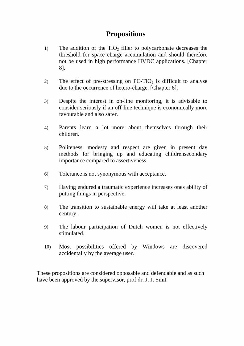
Propositions 1) The addition of the TiO2 filler to polycarbonate decreases the
threshold for space charge accumulation and should therefore not be used in high performance HVDC applications. [Chapter 8].
2) The effect of pre-stressing on PC-TiO2 is difficult to analyse
due to the occurrence of hetero-charge. [Chapter 8].
3) Despite the interest in on-line monitoring, it is advisable to consider seriously if an off-line technique is economically more favourable and also safer.
4) Parents learn a lot more about themselves through their
children.
5) Politeness, modesty and respect are given in present day methods for bringing up and educating childrensecondary importance compared to assertiveness.
6) Tolerance is not synonymous with acceptance.
7) Having endured a traumatic experience increases ones ability of
putting things in perspective.
8) The transition to sustainable energy will take at least another century.
9) The labour participation of Dutch women is not effectively
stimulated.
10) Most possibilities offered by Windows are discovered accidentally by the average user.
These propositions are considered opposable and defendable and as such have been approved by the supervisor, prof.dr. J. J. Smit.