DIDACTIC EXPERIMENTS FOR DETERMINING THE SPEED · PDF fileDIDACTIC EXPERIMENTS FOR DETERMINING THE SPEED ... 3 Didactic experiments for determining the speed of sound in the air 1623

Romanian Reports in Physics, Vol. 68, No. 4, P. 1621–1640, 2016

DIDACTIC EXPERIMENTS FOR DETERMINING THE SPEED

OF SOUND IN THE AIR

M. OPREA1,2, CRISTINA MIRON1*

1 University of Bucharest, Faculty of Physics, Bucharest, Romania 2 “Mihai Viteazu” School, Călărași, Romania

E-mail: [email protected]

Received July 2, 2015

Abstract. In this article we set out to design, develop and test didactic experiments for

the determination of the speed of sound in the air and to compare the didactic efficacy

of these experiments. Firstly, we analysed the methods based on measuring the time

interval after which the sound reflected by an obstacle is detected. Secondly, we

presented the methods of measuring the time of flight of an acoustic wave front

between two detectors (microphones). The first category of didactic experiments

(echo recording) contains sound speed determinations using an ultrasonic sensor

connected to an Arduino processing board, the reflection on one end closed tubes and

the reflection on walls situated within a large distance from the sound source. The

second category of didactic experiments (time of flight recordings) contains

determinations using a data acquisition device (NIDAQ).

Key words: sound, speed, Ping sensor, Arduino, tube, microphone, echo, data

acquisition device, LabVIEW, Audacity.

1. INTRODUCTION

A very important teaching-related aspect of the experimental activities

associated with the study of Acoustics concerns the measuring the speed of sound

through the air. Literature in this field comprises a series of studies [1, 2, 3], such

as the study of Berg and Courtney [4] about the echo-based method of measuring

the speed of the sound, the determinations performed by Litwhiler and Lovell [5]

with the help of a computer sound card and a LabVIEW software application, as

well as the determinations made by Carvalho et al. [6] with free software

application, such as Audacity.

However, such studies do not perform a comparative analysis of these

methods in order to test the efficiency of each one. That is why this paper brings

forward a new approach, by testing a wide methodical spectrum and emphasizing,

comparatively, the quality factors that differentiate the degree of efficiency of these

methods. The factors that we made reference to were: the financial investment

needed to acquire the experimental materials, the time required to perform the

mailto:%[email protected]

1622 M. Oprea, Cristina Miron 2

experiment, the minimum digital competence level of the students, the time for

data processing and last, but not least, the precision of the measurements

performed.

2. DETERMINATION OF THE SPEED OF SOUND THROUGH THE AIR

USING THE ECHO-BASED METHOD

The common principle of these methods consists in emitting a sound wave

towards a wall and receiving the echo produced (Fig. 1). Measuring the time lag

( t ) between the moment when the sound was emitted and the moment it was

received we can calculate the speed of the sound ( sv ) based on the mathematical

relation:

t

dvs

2, (1)

where d represents the value of the distance between the sound source and the

wall.

Fig. 1 – Schematic representation of the methodic principle used to determine the speed of sound

through the “echo-based method”. The colored versions can be accessed at http://www.infim.ro/rrp/.

This method of determining the speed of sound in the air was used for three

different distances: short distance [cm], medium distance [m], long distance

(dozens of meters).

2.1. DETERMINING THE SPEED OF SOUND IN THE AIR THROUGH ECHO-BASED

METHODS USING A SHORT RANGE ULTRASONIC SENSOR

We used an ultrasonic sensor Ping connected to a development Arduino

board (Fig. 2).

http://www.infim.ro/rrp/

3 Didactic experiments for determining the speed of sound in the air 1623

Fig. 2 – Experimental scheme for a short range ultrasonic sensor.

The colored versions can be accessed at http://www.infim.ro/rrp/.

This sensor has a range of action from 2 cm to 3 m. The functional control of

the sensor is done through an application uploaded on Arduino. Therefore, the

sensor is programmed to emit an ultrasonic impulse (on the 40 kHz frequency) and

detect the echo produced by an object situated on the direction of the ultrasonic

flow. The application measures the time lag emission-reception ( t ) and, knowing

the distance relative to the object d , can determine sv according the the relation

(1). The aspects associated with the experimental setup, the diagram of the

application and the results obtained can be seen in the images below (Figs. 3–6).

Fig. 3 – Experimental setup.

The colored versions can be accessed at

http://www.infim.ro/rrp/.

Fig. 4 – Experimental values obtained.







Fig. 5 – Sequences from the Arduino application diagram.


Fig. 6 – Monitoring of the obtained values.


We performed measurements of sv for different distances between the sensor

and the objects situated in its vicinity, under various conditions of temperature and

humidity of the surrounding environment.

The experimental results of sv for different accoustically reflective physical

environments are illustrated in Table 1. We used the following notations:

d – distance; t – time; sv – sound speed; srv – reference value sound speed;

smv – medium value sound speed; srmv – medium value reference sound speed;

– measurement error; m – medium measurement error; r – relative

measurement error; rm – medium relative error; – temperature; RH – relative

humidity index.

The reference values of the speed of sound through the air, were established

using the relation (2):




s

mvsr )600.0331( m/s. (2)

Table 1

Experimental results of sv for different accoustically reflective physical environments

Material d

(cm) t

(μs) sv

(m/s)

srv

(m/s)

smv

(m/s)

srmv

(m/s)

sm srmv v

sm srmv v

(m/s)

m

(m/s) srm

srmsmr

v

vv

(%)

rm

(%)

(oC)

RH

(%)

PVC

10 593 337.3 344.2

339.8 347 7.2

8.06

2.07

2.32

22 52

10 589 339.6 346.6 26 68

10 584 342.5 350.2 32 79

metal

50 2975 336.1 344.2

338.7 347 8.3 2.39

22 52

50 2950 338.9 346.6 26 68

50 2930 341.2 350.2 32 79

concrete

60 3573 335.9 344.2

338.3 347 8.7 2.50

22 52

120 7092 338.4 346.6 26 68

240 14088 340.7 350.2 32 79

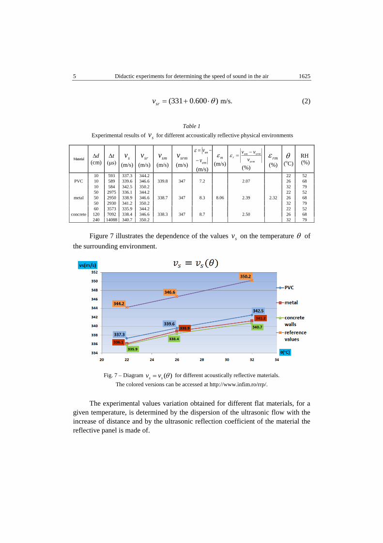
Figure 7 illustrates the dependence of the values sv on the temperature of

the surrounding environment.

Fig. 7 – Diagram )(ss vv for different acoustically reflective materials.


The experimental values variation obtained for different flat materials, for a

given temperature, is determined by the dispersion of the ultrasonic flow with the

increase of distance and by the ultrasonic reflection coefficient of the material the

reflective panel is made of.



Analysing the graphic of dependence )(ss vv for the plastic reflective

wall (Fig. 8) we deducted a medium value of its slope 575.0m rather close to the

value 600.0m associated to the reference speed value graph from the same

diagram. Therefore, the equations of the two lines )(ss vv and )(srsr vv are:

575.0326

600.0331

s

sr

v

v. (3)

Fig. 8 – Graphical representations )(ss vv , )(srsr vv . The colored versions can be accessed at


The analysis of the experimental data on the thermal interval ( C3222oC)

indicates a medium value measured for the sound speed s

mvsm 9.338 m/s related to

the medium value reference s

mvsrm 347 m/s. With a relative medium error

%32.2rm , we deduce the fact that such measurements have a good precision,

adapted for didactic purposes.


METHODS ON A MEDIUM RANGE DISTANCE

In this experiment we used a small section tube [cm2] of known length L ,

closed at one end. At the other end of the tube we placed a sensitive microphone,

connected to the sound card of a computer (Fig. 9).



Fig. 9 – Experimental scheme using a tube closed at one end.


An acoustic signal was generated next to the microphone. The acoustic wave

emitted was detected by the microphone and turned into an electric signal, digitally

processed by sound editing software installed on a PC (Audacity – free audio

editor). The acoustic wave front propagated towards the inside of the tube and,

when reaching its closed end, reflected back towards the microphone. The

microphone recorded a second signal, which was sent to the computer. The time

interval between the two detected signals was calculated from the graphic analysis

of the electrical wave forms displayed in the window of the audio editing software.

Knowing the length of the acoustic reflection tube ( L ) and the time interval

between the main wave front and the reflected one ( t ), the speed of the sound

( sv ) was calculated based on the relation:

t

Lvs

2. (4)

We performed experiments using tubes made of different materials (PVC,

metal), having different values of the cross-sections and of their lengths (Fig. 10–13).

Fig. 10 – Experimental setup using a PVC tube (L = 1 m).





Fig. 11 – Experimental setup using a long PVC tube (L = 3 m).


Fig. 12 – Experimental setup using an aluminum tube (L = 0.85 m).


Fig. 13 – Experimental setup using a copper tube (L = 1 m).


In the following diagrams (Figs. 14–16) we can observe a few results from

the set of experimental data obtained:





Fig. 14 – Experimental results for a PVC tube.


Fig. 15 – Experimental results for an aluminum tube.


Fig. 16 – Experimental results for a copper tube.


The experiments were performed in various conditions of the thermodynamic

atmospheric parameters: temperature and humidity.





The obtained results can be visualized in Table 2.

Table 2

Experimental results for sv obtained for tubes of various materials closed at one end

Material L

(cm)

(cm)

t

(ms) sv

(m/s)

srv

(m/s)

smv

(m/s)

srmv

(m/s)

srmsm vv

srmsm vv

(m/s)

m

(m/s) srm

srmsmr

v

vv

(%)

rm (%) )( C

(oC)

RH

(%)

PVC tube

100 5 5.76 347.2 346

346.5 348.23 1.73

2.02

0.49

0.57

25 55

100 2 8.66 346.4 348.5 29 64

200 1.5 11.55 346.02 350.2 32 70

Metallic

tube

Cu 100 1 5.73 349.04 346 349.04 346 3.04 0.87 25 55

Al 87 3 5.01 347.3 346 347.3 346 1.3 0.37 25 55

The notations L and correspond to the lengths and to the diameters of the

selected tubes.

One could notice an insignificant dependence of the value sv on the tube

section (S) or its length (L). However, the resolution of the reflection diagram is

more visible for long tubes with a wider section. The experimental data, recorded

in the thermal interval (25 C3225 32 oC), indicate a medium measured value of the speed

of sound s

mvsm 6.347 m/s related to a medium reference value

s

mvsrm 7.346 m/s. The

presence of a value %1rm leads to the conclusion that such an experimental

method is recommended for high precision measurements of the speed of sound in

the air.


METHODS ON A LONG RANGE DISTANCE

As a sound source we used a balloon (containing air at high pressure) situated

near a directive microphone (having a parabolic reflector) facing the wall and

connected to the sound card of a computer. The sudden release of the air contained

in the balloon generates an acoustic wave which propagates omnidirectionally. The

acoustic disturbance is detected by the microphone in two stages: at first, directly

and, a little later, through reflection on a wall situated at an established distance

d (Fig. 17).

The audio editing software displays the wave forms of the two signals in a

time domain diagram. Knowing the distance acoustic source – wall d and

determining the time interval t between the direct signal and the reflected signal

allows us to apply the formula (1) and determine sv .


Fig. 17 – Experimental scheme using the echo-based method on a wall.


The experiments were performed outside (schoolyard) using the sound

reflection on the wall of a building (school) (Figs. 18 and 19).

.

Fig. 18 – Experimental setup (front view).


Fig. 19 – Experimental setup (back view).






In Fig. 20 there is an example of an Audacity diagram containing a recording

st 099.0 s for the spatial interval md 17 m.

Fig. 20 – Time interval recording t .


In Table 3 one can observe aspects of the experimental recordings.

Table 3

Experimental results of sv obtained using the “echo on a wall” method

Area d

(m)

t

(ms) sv

(m/s)

srv

(m/s)

smv

(m/s)

srmsm vv

srmsm vv

(m/s)

srm

srmsmr

v

vv

(%)

)( C

(oC)

RH

(%)

Outdoor (schoolyard)

17 9.9 343.43

346 342.5 3.5 1.01 25 65 50 29.2 342.46

75 43.9 341.6

The experiments took place in constant temperature and atmospheric pressure

conditions. The method has a good accuracy, in direct proportion to the sesitivity

and acoustic directivity of the microphone in use. The medium value of the speed

of sound s

mvs 5.342 m/s is rather close to the reference value

s

mvsr 346 m/s. The

presence of multiple echoes requires a high resolution analysis of the wave forms

associated with the signals recorded by a microphone, in order to establish the

precise temporal interval needed to determine sv .



3. METHODS BASED ON DETERMINING THE TIME OF FLIGHT

Through these methods we can determine the value of the time interval t in

which an acoustic wave front emitted by a source placed next to a microphone is

propagated towards another microphone situated at a distance d from the first.

The acoustic signals detected by the microphones are digitally processed through a

specialized software so that we can measure the time lag between them: t .

Knowing the values of d and t we can determine sv based on the relation:

t

dvs

. (5)

3.1. DETERMINING THE TIME OF FLIGHT USING WALKIE-TALKIE STATIONS

(OUTDOOR METHOD)

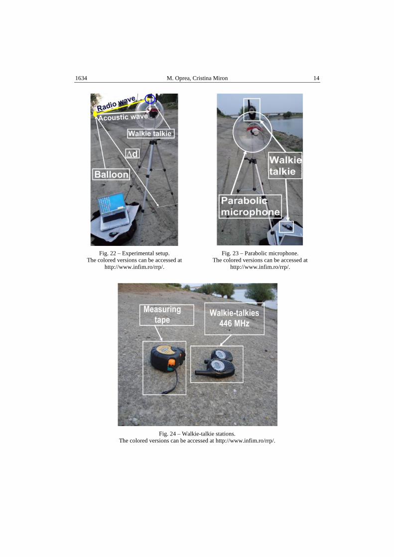
This method uses two walkie-talkies, a microphone with a parabolic reflector and on overpressurised balloon. The walkie-talkie stations were configured on the same communication channel. The microphone was connected to a laptop on which the sound recording and editing application Audacity was used (Fig. 21). Two operators were needed for the successful completion of this experiment. One of them moved with a walkie-talkie and with the balloon at a considerable distance (a few hundred meters) from the place where the other operator was located. The latter placed the walkie-talkie near the microphone and started the sound recording application (Figs. 22–24). The sudden release of air from the balloon (through explosion) generated an acoustic disturbance that was detected by the walkie-talkie and transmitted, through the radio communication channel, to the other station. This station emitted a signal upon reception which was detected and recorded by

the parabolic microphone. After a time interval t , the acoustic wave front arrived, propagated through the air. This second signal was also recorded.

Analysing the graphic which contains the recorded wave forms we

determined, with a good degree of accuracy, the value of t (Fig. 25). Measuring

the distance between the two walkie-talkies ( d ), we calculated the value of the speed of sound based on the relation (5).

Fig. 21 – Experimental scheme for determining the time of flight using walkie-talkies.







Fig. 23 – Parabolic microphone.



Fig. 24 – Walkie-talkie stations.






Fig. 25 – Determination of t and sv for d = 375 m.


Table 4 contains a few experimental results.

Table 4

Experimental results of sv using the outdoor method

d

(m)

t

(s) sv

(m/s)

srv

(m/s) smv

(m/s)

srmsm vv

(m/s) srm

srmsmr

v

vv

(%)

)( C

(oC)

RH

(%)

300 0.885 339

345.4 336.6 9 2.6 25 63 375 1.115 336.3

450 1.345 334.6

The recordings performed under constant pressure, temperature and humidity

led to a medium value of s

mvs 6.336 m/s, related to a reference value

s

mvsr 4.345 m/s.

The method employed is efficient (relative error %6.2r ) and interesting,

because it emphasizes two speeds at which the information may propagate: the

radio waves speed (speed of light) and the acoustic wave speed (speed of sound).

The resolution t (between the two detected signals) is good, due to the high

distance travelled by the acoustic wave front.

3.2. METHOD OF DETERMINING t USING A DATA ACQUISITION DEVICE

(INDOOR METHOD)

In this experiment the two microphones for sound detection were set up at a

distance of a few meters from each other. We used two data channels from the data

acquistion device NIDAQ 6008. The signals detected by the microphones were



amplified and acquired by the data entry channels, being digitally processed using

LabVIEW Signal Express. As an acoustic signal source we used an overpressurized

balloon. The explosion of the balloon near one of the microphones generated an

acoustic wave that propagated towards the other microphone (Figs. 26–28).

Fig. 26 – Experimental scheme for determining t using a data acquisition device.




Fig. 28 – DAQ signal recording.






The analysis made by the data acquisition device allows the measurement of

the time interval in which the acoustic disturbance travels between the two

detectors (Fig. 29 and Fig. 30).

Fig. 29 – Time domain signal analysis.


Fig. 30 – Time interval t measurement.


One can notice in Table 5 examples of experimental recordings.

The medium measured value of the speed of sound through this method was

s

mvs 57.350 m/s, related to a reference value

s

mvsr 4.348 m/s. The relatively small

error (under 1%) makes this method suitable for high precision measurements of

the value sv .




Table 5

Examples of experimental recordings using the indoor method

d

(m)

t

(ms) sv

(m/s)

srv

(m/s) smv

(m/s)

srmsm vv

(m/s) srm

srmsmr

v

vv

(%)

)( C

(oC)

RH

(%)

1 2.84 352.11

348.4 350.57 2.17 0.6 29 70 2 5.71 350.26

4 11.45 349.34

4. CONCLUSIONS

The conclusions of the comparison involving the experiment-based methods

presented in this article can be drawn based on the data found in Table 6. We used

quality indexes for the methodical evaluation criteria present in the table (L – low,

M – middle, H – high). We proceeded to attribute values to those indexes, ranging

on a scale from 1 to 10, as follows: L – interval 41 ; M – interval 75 ; H –

interval 108 .

The score for the applicability of each method in Physics Education was

calculated based on the formula:

DA

.VFI+TPE+DCR+DPT

S (6)

The variables present in the algebraic structure of the formula are illustrated

in Table 6 and the graphic representation in Fig. 31.

Table 6

Compared analysis of methods

Methodical evaluation criteria

Methods

Echo Time of flight

Ultrasounds Tubes Walls Walkie-talkies DAQ

Financial investment value (FIV) H8 M7 M5 H8 H10

Time required to perform experiment

(TPE) L2 L3 M7

H9 M7

Digital competences required (DCR) H9 M7 M7 M7 H9

Data processing time (DPT) L1 M7 M7 M7 M7

Data accuracy (DA) H8 H9 H8 H8 H9

Score for method applicability in

class (S) 0.400 0.375 0.307 0.258 0.272


Fig. 31 – Methodology rating. The colored versions can be accessed at http://www.infim.ro/rrp/.

Analysing the values of S for the echo-based method, we concluded that the

experiments based on ultrasonic echoes rank first, followed closely by the tubes

experiments. In what concerns the time of flight method, the leading experiments

are those involving the use of a data acquisition device (NIDAQ). Whichever of

these methods can be successfully applied in Physics Education, conveying results

that allow for both a qualitative and quantitative approach in the sound speed

measuring experiments. All in all, as we have shown in previous studies [7, 8], in

line with the findings of other authors [9, 10], the role of experiments in the

teaching of physical concepts or phenomena is of outmost importance, arising

students’ awareness and curiosity towards the topics that are investigated.

REFERENCES

1. B. E. Martin, Measuring the speed of sound: variation on a familiar theme, Phys. Teach. 39, 424

(2001).

2. H. N. Ali, Measurement of The Speed of Sound, LUMS School of Science and Engineering, July

24, 2009.

3. G. B. Karshner, Direct method for measuring the speed of sound, Am. J. Phys. 57, 920 (1989).

4. A. Berg and M. Courtney, Echo-based measurement of the speed of sound, Popular Physics,

Cornell University Library, February 2011.

5. D.H. Litwhiler and T.D. Lovell, Acoustic Measurements Using Common Computer Accessories:

Do Try This at Home, Proceedings of the American Society for Engineering Education Annual

Conference and Exposition, 2005.

6. C. C. Carvalho, J. M. B. Lopes dos Santos and M. B. Marques, A time of flight method to

measure the speed of sound using a stereo sound card, Phys. Teach. 46, 428 (2008).

7. M. Oprea and C. Miron, Mobile Phones in the Modern Teaching of Physics, Romanian Reports

in Physics 66, 4, 1236–1252 (2014).

8. M. Oprea and C. Miron, Applied Physics Projects Using the Arduino Platform, Proceedings of

the 8th International Conference on Virtual Learning ICVL, Bucharest, 2013, pp. 204–210.

9. Z. Hrepic, D. Zollman and S. Rebello, Identifying students' models of sound propagation,

Physics Education Research Conference, 2002, Boise ID.

10. C.J. Linder, Understanding sound: So what is the problem?, Physics Education 27, 5, 258–264.


Documents

DIDACTIC EXPERIMENTS FOR DETERMINING THE SPEED · PDF fileDIDACTIC EXPERIMENTS FOR DETERMINING THE SPEED ... 3 Didactic experiments for determining the speed of sound in the air 1623