Embed Size (px)
Citation preview
LETTER Communicated by Hagai Attias
Dictionary Learning Algorithms for Sparse Representation
Kenneth [email protected] F. [email protected] D. [email protected] and Computer Engineering, Jacobs School of Engineering,University of California, San Diego, La Jolla, California 92093-0407, U.S.A.
Kjersti [email protected] University College, School of Science and Technology Ullandhaug,N-4091 Stavanger, Norway
Te-Won [email protected] J. [email protected] Hughes Medical Institute, Computational Neurobiology Laboratory,Salk Institute, La Jolla, California 92037, U.S.A.
Algorithms for data-driven learning of domain-specific overcomplete dic-tionaries are developed to obtain maximum likelihood and maximuma posteriori dictionary estimates based on the use of Bayesian modelswith concave/Schur-concave (CSC) negative log priors. Such priors are ap-propriate for obtaining sparse representations of environmental signalswithin an appropriately chosen (environmentally matched) dictionary.The elements of the dictionary can be interpreted as concepts, features,or words capable of succinct expression of events encountered in the en-vironment (the source of the measured signals). This is a generalizationof vector quantization in that one is interested in a description involv-ing a few dictionary entries (the proverbial “25 words or less”), but notnecessarily as succinct as one entry. To learn an environmentally adapteddictionary capable of concise expression of signals generated by the envi-ronment, we develop algorithms that iterate between a representative setof sparse representations found by variants of FOCUSS and an update ofthe dictionary using these sparse representations.
Experiments were performed using synthetic data and natural images.For complete dictionaries, we demonstrate that our algorithms have im-
Neural Computation 15, 349–396 (2003) c© 2002 Massachusetts Institute of Technology
350 K. Kreutz-Delgado, J. Murray, B. Rao, K. Engan, T. Lee, and T. Sejnowski
proved performance over other independent component analysis (ICA)methods, measured in terms of signal-to-noise ratios of separated sources.In the overcomplete case, we show that the true underlying dictionary andsparse sources can be accurately recovered. In tests with natural images,learned overcomplete dictionaries are shown to have higher coding effi-ciency than complete dictionaries; that is, images encoded with an over-complete dictionary have both higher compression (fewer bits per pixel)and higher accuracy (lower mean square error).
1 Introduction
FOCUSS, which stands for FOCal Underdetermined System Solver, is analgorithm designed to obtain suboptimally (and, at times, maximally) sparsesolutions to the following m× n, underdetermined linear inverse problem1
(Gorodnitsky, George, & Rao, 1995; Rao & Gorodnitsky, 1997; Gorodnitsky& Rao, 1997; Adler, Rao, & Kreutz-Delgado, 1996; Rao & Kreutz-Delgado,1997; Rao, 1997, 1998),
y = Ax, (1.1)
for known A. The sparsity of a vector is the number of zero-valued ele-ments (Donoho, 1994), and is related to the diversity, the number of nonzeroelements,
sparsity = #{x[i] = 0}diversity = #{x[i] �= 0}diversity = n− sparsity.
Since our initial investigations into the properties of FOCUSS as an al-gorithm for providing sparse solutions to linear inverse problems in rel-atively noise-free environments (Gorodnitsky et al., 1995; Rao, 1997; Rao& Gorodnitsky, 1997; Gorodnitsky & Rao, 1997; Adler et al., 1996; Rao &Kreutz-Delgado, 1997), we now better understand the behavior of FOCUSSin noisy environments (Rao & Kreutz-Delgado, 1998a, 1998b) and as an in-terior point-like optimization algorithm for optimizing concave functionalssubject to linear constraints (Rao & Kreutz-Delgado, 1999; Kreutz-Delgado& Rao, 1997, 1998a, 1998b, 1998c, 1999; Kreutz-Delgado, Rao, Engan, Lee, &Sejnowski, 1999a; Engan, Rao, & Kreutz-Delgado, 2000; Rao, Engan, Cotter,& Kreutz-Delgado, 2002). In this article, we consider the use of the FO-CUSS algorithm in the case where the matrix A is unknown and must belearned. Toward this end, we first briefly discuss how the use of concave (and
1 For notational simplicity, we consider the real case only.
Dictionary Learning Algorithms for Sparse Representation 351
Schur concave) functionals enforces sparse solutions to equation 1.1. We alsodiscuss the choice of the matrix, A, in equation 1.1 and its relationship tothe set of signal vectors y for which we hope to obtain sparse representa-tions. Finally, we present algorithms capable of learning an environmentallyadapted dictionary, A, given a sufficiently large and statistically represen-tative sample of signal vectors, y, building on ideas originally presented inKreutz-Delgado, Rao, Engan, Lee, and Sejnowski (1999b), Kreutz-Delgado,Rao, and Engan (1999), and Engan, Rao, and Kreutz-Delgado (1999).
We refer to the columns of the full row-rank m× n matrix A,
A = [a1, . . . , an] ∈ Rm×n, n m, (1.2)
as a dictionary, and they are assumed to be a set of vectors capable of provid-ing a highly succinct representation for most (and, ideally, all) statisticallyrepresentative signal vectors y ∈ R
m. Note that with the assumption thatrank(A) = m, every vector y has a representation; the question at hand iswhether this representation is likely to be sparse. We call the statistical gen-erating mechanism for signals, y, the environment and a dictionary, A, withinwhich such signals can be sparsely represented an environmentally adapteddictionary.
Environmentally generated signals typically have significant statisticalstructure and can be represented by a set of basis vectors spanning a lower-dimensional submanifold of meaningful signals (Field, 1994; Ruderman,1994). These environmentally meaningful representation vectors can be ob-tained by maximizing the mutual information between the set of these vec-tors (the dictionary) and the signals generated by the environment (Comon,1994; Bell & Sejnowski, 1995; Deco & Obradovic, 1996; Olshausen & Field,1996; Zhu, Wu, & Mumford, 1997; Wang, Lee, & Juang, 1997). This proce-dure can be viewed as a natural generalization of independent componentanalysis (ICA) (Comon, 1994; Deco & Obradovic, 1996). As initially devel-oped, this procedure usually results in obtaining a minimal spanning setof linearly independent vectors (i.e., a true basis). More recently, the desir-ability of obtaining “overcomplete” sets of vectors (or “dictionaries”) hasbeen noted (Olshausen & Field, 1996; Lewicki & Sejnowski, 2000; Coifman& Wickerhauser, 1992; Mallat & Zhang, 1993; Donoho, 1994; Rao & Kreutz-Delgado, 1997). For example, projecting measured noisy signals onto thesignal submanifold spanned by a set of dictionary vectors results in noisereduction and data compression (Donoho, 1994, 1995). These dictionariescan be structured as a set of bases from which a single basis is to be selected torepresent the measured signal(s) of interest (Coifman & Wickerhauser, 1992)or as a single, overcomplete set of individual vectors from within which avector, y, is to be sparsely represented (Mallat & Zhang, 1993; Olshausen &Field, 1996; Lewicki & Sejnowski, 2000; Rao & Kreutz-Delgado, 1997).
The problem of determining a representation from a full row-rank over-complete dictionary, A = [a1, . . . , an], n m, for a specific signal mea-
352 K. Kreutz-Delgado, J. Murray, B. Rao, K. Engan, T. Lee, and T. Sejnowski
surement, y, is equivalent to solving an underdetermined inverse problem,Ax = y, which is nonuniquely solvable for any y. The standard least-squaressolution to this problem has the (at times) undesirable feature of involv-ing all the dictionary vectors in the solution2 (the “spurious artifact” prob-lem) and does not generally allow for the extraction of a categorically orphysically meaningful solution. That is, it is not generally the case that aleast-squares solution yields a concise representation allowing for a precisesemantic meaning.3 If the dictionary is large and rich enough in representa-tional power, a measured signal can be matched to a very few (perhaps evenjust one) dictionary words. In this manner, we can obtain concise seman-tic content about objects or situations encountered in natural environments(Field, 1994). Thus, there has been significant interest in finding sparse so-lutions, x (solutions having a minimum number of nonzero elements), tothe signal representation problem. Interestingly, matching a specific signalto a sparse set of dictionary words or vectors can be related to entropy min-imization as a means of elucidating statistical structure (Watanabe, 1981).Finding a sparse representation (based on the use of a “few” code or dictio-nary words) can also be viewed as a generalization of vector quantizationwhere a match to a single “code vector” (word) is always sought (taking“code book” = “dictionary”).4 Indeed, we can refer to a sparse solution, x,as a sparse coding of the signal instantiation, y.
1.1 Stochastic Models. It is well known (Basilevsky, 1994) that the sto-chastic generative model
y = Ax+ ν, (1.3)
can be used to develop algorithms enabling coding of y ∈ Rm via solving
the inverse problem for a sparse solution x ∈ Rn for the undercomplete
(n < m) and complete (n = m) cases. In recent years, there has been a greatdeal of interest in obtaining sparse codings of y with this procedure for theovercomplete (n > m) case (Mallat & Zhang, 1993; Field, 1994). In our earlierwork, we have shown that given an overcomplete dictionary, A (with thecolumns of A comprising the dictionary vectors), a maximum a posteriori(MAP) estimate of the source vector, x, will yield a sparse coding of y inthe low-noise limit if the negative log prior, − log(P(x)), is concave/Schur-concave (CSC) (Rao, 1998; Kreutz-Delgado & Rao, 1999), as discussed below.
2 This fact comes as no surprise when the solution is interpreted within a Bayesianframework using a gaussian (maximum entropy) prior.
3 Taking “semantic” here to mean categorically or physically interpretable.4 For example, n = 100 corresponds to 100 features encoded via vector quantization
(“one column = one concept”). If we are allowed to represent features using up to four
columns, we can encode
(100
1
)+(
1002
)+(
1003
)+(
1004
)= 4,087,975 concepts showing
a combinatorial boost in expressive power.
Dictionary Learning Algorithms for Sparse Representation 353
For P(x) factorizable into a product of marginal probabilities, the resultingcode is also known to provide an independent component analysis (ICA)representation of y. More generally, a CSC prior results in a sparse represen-tation even in the nonfactorizable case (with x then forming a dependentcomponent analysis, or DCA, representation).
Given independently and identically distributed (i.i.d.) data, Y = YN =(y1, . . . , yN), assumed to be generated by the model 1.3, a maximum likeli-hood estimate, AML, of the unknown (but nonrandom) dictionary A can bedetermined as (Olshausen & Field, 1996; Lewicki & Sejnowski, 2000)
AML = arg maxA
P(Y;A).
This requires integrating out the unobservable i.i.d. source vectors, X =XN = (x1, . . . , xN), in order to compute P(Y;A) from the (assumed) knownprobabilities P(x) and P(ν). In essence, X is formally treated as a set ofnuisance parameters that in principle can be removed by integration. How-ever, because the prior P(x) is generally taken to be supergaussian, thisintegration is intractable or computationally unreasonable. Thus, approxi-mations to this integration are performed that result in an approximationto P(Y;A), which is then maximized with respect to Y. A new, better ap-proximation to the integration can then be made, and this process is iterateduntil the estimate of the dictionary A has (hopefully) converged (Olshausen& Field, 1996). We refer to the resulting estimate as an approximate maxi-mum likelihood (AML) estimate of the dictionary A (denoted here by AAML).No formal proof of the convergence of this algorithm to the true maxi-mum likelihood estimate, AML, has been given in the prior literature, butit appears to perform well in various test cases (Olshausen & Field, 1996).Below, we discuss the problem of dictionary learning within the frame-work of our recently developed log-prior model-based sparse source vectorlearning approach that for a known overcomplete dictionary can be used toobtain sparse codes (Rao, 1998; Kreutz-Delgado & Rao, 1997, 1998b, 1998c,1999; Rao & Kreutz-Delgado, 1999). Such sparse codes can be found usingFOCUSS, an affine scaling transformation (AST)–like iterative algorithmthat finds a sparse locally optimal MAP estimate of the source vector xfor an observation y. Using these results, we can develop dictionary learn-ing algorithms within the AML framework and for obtaining a MAP-likeestimate, AMAP, of the (now assumed random) dictionary, A, assuming inthe latter case that the dictionary belongs to a compact submanifold corre-sponding to unit Frobenius norm. Under certain conditions, convergenceto a local minimum of a MAP-loss function that combines functions of thediscrepancy e = (y − Ax) and the degree of sparsity in x can be rigorouslyproved.
1.2 Related Work. Previous work includes efforts to solve equation 1.3in the overcomplete case within the maximum likelihood (ML) framework.
354 K. Kreutz-Delgado, J. Murray, B. Rao, K. Engan, T. Lee, and T. Sejnowski
An algorithm for finding sparse codes was developed in Olshausen andField (1997) and tested on small patches of natural images, resulting inGabor-like receptive fields. In Lewicki and Sejnowski (2000) another MLalgorithm is presented, which uses the Laplacian prior to enforce sparsity.The values of the elements of x are found with a modified conjugate gradientoptimization (which has a rather complicated implementation) as opposedto the standard ICA (square mixing matrix) case where the coefficients arefound by inverting the A matrix. The difficulty that arises when using MLis that finding the estimate of the dictionary A requires integrating over allpossible values of the joint density P(y, x;A) as a function of x. In Olshausenand Field (1997), this is handled by assuming the prior density of x is a deltafunction, while in Lewicki and Sejnowski (2000), it is approximated by agaussian. The fixed-point FastICA (Hyvarinen, Cristescu, & Oja, 1999) hasalso been extended to generate overcomplete representations. The FastICAalgorithm can find the basis functions (columns of the dictionary A) oneat a time by imposing a quasi-orthogonality condition and can be thoughtof as a “greedy” algorithm. It also can be run in parallel, meaning that allcolumns of A are updated together.
Other methods to solve equation 1.3 in the overcomplete case have beendeveloped using a combination of the expectation-maximization (EM) algo-rithm and variational approximation techniques. Independent factor anal-ysis (Attias, 1999) uses a mixture of gaussians to approximate the priordensity of the sources, which avoids the difficulty of integrating out theparameters X and allows different sources to have different densities. Inanother method (Girolami, 2001), the source priors are assumed to be su-pergaussian (heavy-tailed), and a variational lower bound is developed thatis used in the EM estimation of the parameters A and X. It is noted in Giro-lami (2001) that the mixtures used in independent factor analysis are moregeneral than may be needed for the sparse overcomplete case, and theycan be computationally expensive as the dimension of the data vector andnumber of mixtures increases.
In Zibulevsky and Pearlmutter (2001), the blind source separation prob-lem is formulated in terms of a sparse source underlying each unmixedsignal. These sparse sources are expanded into the unmixed signal with apredefined wavelet dictionary, which may be overcomplete. The unmixedsignals are linearly combined by a different mixing matrix to create theobserved sensor signals. The method is shown to give better separationperformance than ICA techniques. The use of learned dictionaries (insteadof being chosen a priori) is suggested.
2 FOCUSS: Sparse Solutions for Known Dictionaries
2.1 Known Dictionary Model. A Bayesian interpretation is obtainedfrom the generative signal model, equation 1.3, by assuming that x has the
Dictionary Learning Algorithms for Sparse Representation 355
parameterized (generally nongaussian) probability density function (pdf),
Pp(x) = Z−1p e−γpdp(x), Zp =
∫e−γpdp(x) dx, (2.1)
with parameter vector p. Similarly, the noise ν is assumed to have a param-eterized (possibly nongaussian) density Pq(ν) of the same form as equa-tion 2.1 with parameter vector q. It is assumed that x and ν have zero meansand that their densities obey the property d(x) = d(|x|), for | · | definedcomponent-wise. This is equivalent to assuming that the densities are sym-metric with respect to sign changes in the components x, x[i] ← −x[i] andtherefore that the skews of these densities are zero. We also assume thatd(0) = 0. With a slight abuse of notation, we allow the differing subscriptsq and p to indicate that dq and dp may be functionally different as well asparametrically different. We refer to densities like equation 2.1 for suitableadditional constraints on dp(x), as hypergeneralized gaussian distributions(Kreutz-Delgado & Rao, 1999; Kreutz-Delgado et al., 1999).
If we treat A, p, and q as known parameters, then x and y are jointlydistributed as
P(x, y) = P(x, y; p, q, A).
Bayes’ rule yields
P(x | y; p, A) = 1β
P(y | x; p, A) · P(x; p, A) = 1β
Pq(y− Ax) · Pp(x) (2.2)
β = P(y) = P(y; p, q, A) =∫
P(y | x) · Pp(x) dx. (2.3)
Usually the dependence on p and q is notationally suppressed, for example,β = P(y;A). Given an observation, y, maximizing equation 2.2 with respectto x yields a MAP estimate x. This ideally results in a sparse coding of theobservation, a requirement that places functional constraints on the pdfs,and particularly on dp. Note that β is independent of x and can be ignoredwhen optimizing equation 2.2 with respect to the unknown source vector x.
The MAP estimate equivalently is obtained from minimizing the negativelogarithm of P(x | y), which is
x = arg minx
dq(y− Ax)+ λdp(x), (2.4)
where λ = γp/γq and dq(y−Ax) = dq(Ax−y) by our assumption of symmetry.The quantity 1
λis interpretable as a signal-to-noise ratio (SNR). Furthermore,
assuming that both dq and dp are concave/Schur–concave (CSC) as defined insection 2.4, then the term dq(y − Ax) in equation 2.4 will encourage sparse
356 K. Kreutz-Delgado, J. Murray, B. Rao, K. Engan, T. Lee, and T. Sejnowski
residuals, e = y− Ax, while the term dp(x) encourages sparse source vectorestimates, x. A given value of λ then determines a trade-off between residualand source vector sparseness.
This most general formulation will not be used here. Although we areinterested in obtaining sparse source vector estimates, we will not enforcesparsity on the residuals but instead, to simplify the development, willassume the q = 2 i.i.d. gaussian measurement noise case (ν gaussian withknown covariance σ 2 · I), which corresponds to taking,
γqdq(y− Ax) = 12σ 2 ‖y− Ax‖2. (2.5)
In this case, problem 2.4 becomes
x = arg minx
12‖y− Ax‖2 + λdp(x). (2.6)
In either case, we note that λ → 0 as γp → 0 which (consistent withthe generative model, 1.3) we refer to as the low noise limit. Because themapping A is assumed to be onto, in the low-noise limit, the optimization,equation 2.4, is equivalent to the linearly constrained problem,
x = arg min dp(x) subject to Ax = y. (2.7)
In the low-noise limit, no sparseness constraint need be placed on the resid-uals, e = y− Ax, which are assumed to be zero. It is evident that the struc-ture of dp(·) is critical for obtaining a sparse coding, x, of the observation y(Kreutz-Delgado & Rao, 1997; Rao & Kreutz-Delgado, 1999). Throughtoutthis article, the quantity dp(x) is always assumed to be CSC (enforcing sparsesolutions to the inverse problem 1.3). As noted, and as will be evident duringthe development of dictionary learning algorithms below, we do not imposea sparsity constraint on the residuals; instead, the measurement noise ν willbe assumed to be gaussian (q = 2).
2.2 Independent Component Analysis and Sparsity Inducing Priors.An important class of densities is given by the generalized gaussians for which
dp(x) = ‖x‖pp =
n∑k=1
|x[k]|p, (2.8)
for p > 0 (Kassam, 1982). This is a special case of the larger p class (thep-class) of functions, which allows p to be negative in value (Rao & Kreutz-Delgado, 1999; Kreutz-Delgado & Rao, 1997). Note that this function hasthe special property of separability,
dp(x) =n∑
k=1
dp(x[k]),
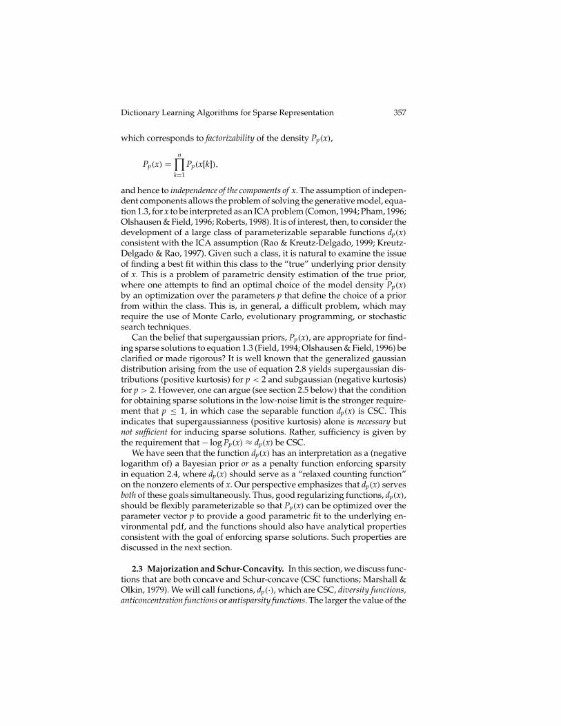
Dictionary Learning Algorithms for Sparse Representation 357
which corresponds to factorizability of the density Pp(x),
Pp(x) =n∏
k=1
Pp(x[k]),
and hence to independence of the components of x. The assumption of indepen-dent components allows the problem of solving the generative model, equa-tion 1.3, for x to be interpreted as an ICA problem (Comon, 1994; Pham, 1996;Olshausen & Field, 1996; Roberts, 1998). It is of interest, then, to consider thedevelopment of a large class of parameterizable separable functions dp(x)
consistent with the ICA assumption (Rao & Kreutz-Delgado, 1999; Kreutz-Delgado & Rao, 1997). Given such a class, it is natural to examine the issueof finding a best fit within this class to the “true” underlying prior densityof x. This is a problem of parametric density estimation of the true prior,where one attempts to find an optimal choice of the model density Pp(x)
by an optimization over the parameters p that define the choice of a priorfrom within the class. This is, in general, a difficult problem, which mayrequire the use of Monte Carlo, evolutionary programming, or stochasticsearch techniques.
Can the belief that supergaussian priors, Pp(x), are appropriate for find-ing sparse solutions to equation 1.3 (Field, 1994; Olshausen & Field, 1996) beclarified or made rigorous? It is well known that the generalized gaussiandistribution arising from the use of equation 2.8 yields supergaussian dis-tributions (positive kurtosis) for p < 2 and subgaussian (negative kurtosis)for p > 2. However, one can argue (see section 2.5 below) that the conditionfor obtaining sparse solutions in the low-noise limit is the stronger require-ment that p ≤ 1, in which case the separable function dp(x) is CSC. Thisindicates that supergaussianness (positive kurtosis) alone is necessary butnot sufficient for inducing sparse solutions. Rather, sufficiency is given bythe requirement that − log Pp(x) ≈ dp(x) be CSC.
We have seen that the function dp(x) has an interpretation as a (negativelogarithm of) a Bayesian prior or as a penalty function enforcing sparsityin equation 2.4, where dp(x) should serve as a “relaxed counting function”on the nonzero elements of x. Our perspective emphasizes that dp(x) servesboth of these goals simultaneously. Thus, good regularizing functions, dp(x),should be flexibly parameterizable so that Pp(x) can be optimized over theparameter vector p to provide a good parametric fit to the underlying en-vironmental pdf, and the functions should also have analytical propertiesconsistent with the goal of enforcing sparse solutions. Such properties arediscussed in the next section.
2.3 Majorization and Schur-Concavity. In this section, we discuss func-tions that are both concave and Schur-concave (CSC functions; Marshall &Olkin, 1979). We will call functions, dp(·), which are CSC, diversity functions,anticoncentration functions or antisparsity functions. The larger the value of the
358 K. Kreutz-Delgado, J. Murray, B. Rao, K. Engan, T. Lee, and T. Sejnowski
CSC function dp(x), the more diverse (i.e., the less concentrated or sparse)the elements of the vector x are. Thus, minimizing dp(x) with respect to xresults in less diverse (more concentrated or sparse) vectors x.
2.3.1 Schur-Concave Functions. A measure of the sparsity of the ele-ments of a solution vector x (or the lack thereof, which we refer to as thediversity of x) is given by a partial ordering on vectors known as the Lorentzorder. For any vector in the positive orthant, x ∈ Rn+, define the decreasingrearrangement
x .= (x�1�, . . . , x�n�), x�1� ≥ · · · ≥ x�n� ≥ 0
and the partial sums (Marshall & Olkin, 1979; Wickerhauser, 1994),
Sx[k] =k∑
i=1
x�n�, k = 1, . . . , n.
We say that y majorizes x, y � x, iff for k = 1, . . . , n,
Sy[k] ≥ Sx[k]; Sy[n] = Sx[n],
and the vector y is said to be more concentrated, or less diverse, than x. Thispartial order defined by majorization then defines the Lorentz order.
We are interested in scalar-valued functions of x that are consistent withmajorization. Such functions are known as Schur-concave functions, d(·): Rn+→ R. They are defined to be precisely the class of functions consistent withthe Lorentz order,
y � x ⇒ d(y) < d(x).
In words, if y is less diverse than x (according to the Lorentz order) then d(y)
is less than d(x) for d(·) Schur-concave. We assume that Schur-concavity is anecessary condition for d(·) to be a good measure of diversity (antisparsity).
2.3.2 Concavity Yields Sparse Solutions. Recall that a function d(·) is con-cave on the positive orthant Rn+ iff (Rockafellar, 1970)
d((1− γ )x+ γy) ≥ (1− γ )d(x)+ γ d(y),
∀x, y ∈ Rn+,∀γ, 0 ≤ γ ≤ 1. In addition, a scalar function is said to be permu-tation invariant if its value is independent of rearrangements of its compo-nents. An important fact is that for permutation invariant functions, con-cavity is a sufficient condition for Schur-concavity:
Concavity+ permutation invariance ⇒ Schur-concavity.
Now consider the low-noise sparse inverse problem, 2.7. It is well knownthat subject to linear constraints, a concave function on Rn+ takes its minima
Dictionary Learning Algorithms for Sparse Representation 359
on the boundary of Rn+ (Rockafellar, 1970), and as a consequence these min-ima are therefore sparse. We take concavity to be a sufficient condition for apermutation invariant d(·) to be a measure of diversity and obtain sparsityas constrained minima of d(·). More generally, a diversity measure shouldbe somewhere between Schur-concave and concave. In this spirit, one candefine almost concave functions (Kreutz-Delgado & Rao, 1997), which areSchur-concave and (locally) concave in all n directions but one, which alsoare good measures of diversity.
2.3.3 Separability, Schur-Concavity, and ICA. The simplest way to en-sure that d(x) be permutation invariant (a necessary condition for Schur-concavity) is to use functions that are separable. Recall that separability ofdp(x) corresponds to factorizability of Pp(x). Thus, separability of d(x) corre-sponds to the assumption of independent components of x under the model1.3. We see that from a Bayesian perspective, separability of d(x) correspondsto a generative model for y that assumes a source, x, with independent com-ponents. With this assumption, we are working within the framework ofICA (Nadal & Parga, 1994; Pham, 1996; Roberts, 1998). We have developedeffective algorithms for solving the optimization problem 2.7 for sparse so-lutions when dp(x) is separable and concave (Kreutz-Delgado & Rao, 1997;Rao & Kreutz-Delgado, 1999).
It is now evident that relaxing the restriction of separability generalizesthe generative model to the case where the source vector, x, has dependentcomponents. We can reasonably call an approach based on a nonsepara-ble diversity measure d(x) a dependent component analysis (DCA). Unlesscare is taken, this relaxation can significantly complicate the analysis anddevelopment of optimization algorithms. However, one can solve the low-noise DCA problem, at least in principle, provided appropriate choices ofnonseparable diversity functions are made.
2.4 Supergaussian Priors and Sparse Coding. The P-class of diversitymeasures for 0 < p ≤ 1 result in sparse solutions to the low-noise codingproblem, 2.7. These separable and concave (and thus Schur-concave) diver-sity measures correspond to supergaussian priors, consistent with the folktheorem that supergaussian priors are sparsity-enforcing priors. However,taking 1 ≤ p < 2 results in supergaussian priors that are not sparsity enforc-ing. Taking p to be between 1 and 2 yields a dp(x) that is convex and thereforenot concave. This is consistent with the well-known fact that for this rangeof p, the pth-root of dp(x) is a norm. Minimizing dp(x) in this case drives x to-ward the origin, favoring concentrated rather than sparse solutions. We seethat if a sparse coding is to be found based on obtaining a MAP estimate tothe low-noise generative model, 1.3, then, in a sense, supergaussianness is anecessary but not sufficient condition for a prior to be sparsity enforcing. Asufficient condition for obtaining a sparse MAP coding is that the negativelog prior be CSC.
360 K. Kreutz-Delgado, J. Murray, B. Rao, K. Engan, T. Lee, and T. Sejnowski
2.5 The FOCUSS Algorithm. Locally optimal solutions to the known-dictionary sparse inverse problems in gaussian noise, equations 2.6 and 2.7,are given by the FOCUSS algorithm. This is an affine-scaling transformation(AST)-like (interior point) algorithm originally proposed for the low-noisecase 2.7 in Rao and Kreutz-Delgado (1997, 1999) and Kreutz-Delgado andRao (1997); and extended by regularization to the nontrivial noise case, equa-tion 2.6, in Rao and Kreutz-Delgado (1998a), Engan et al. (2000), and Rao etal. (2002). In these references, it is shown that the FOCUSS algorithm hasexcellent behavior for concave functions (which includes the the CSC con-centration functions) dp(·). For such functions, FOCUSS quickly convergesto a local minimum, yielding a sparse solution to problems 2.7 and 2.6.
One can quickly motivate the development of the FOCUSS algorithmappropriate for solving the optimization problem 2.6 by considering theproblem of obtaining the stationary points of the objective function. Theseare given as solutions, x∗, to
AT(Ax∗ − y)+ λ∇xdp(x∗) = 0. (2.9)
In general, equation 2.9 is nonlinear and cannot be explicitly solved for asolution x∗. However, we proceed by assuming the existence of a gradientfactorization,
∇xdp(x) = α(x)�(x)x, (2.10)
where α(x) is a positive scalar function and �(x) is symmetric, positive-definite, and diagonal. As discussed in Kreutz-Delgado and Rao (1997,1998c) and Rao and Kreutz-Delgado (1999), this assumption is generallytrue for CSC sparsity functions dp(·) and is key to understanding FOCUSSas a sparsity-inducing interior-point (AST-like) optimization algorithm.5
With the gradient factorization 2.10, the stationary points of equation 2.9are readily shown to be solutions to the (equally nonlinear and implicit)system,
x∗ = (ATA+ β(x∗)�(x∗))−1ATy (2.11)
= �−1(x∗)AT(β(x∗)I + A�−1(x∗)AT)−1y, (2.12)
where β(x) = λα(x) and the second equation follows from identity A.18.Although equation 2.12 is also not generally solvable in closed form, it does
5 This interpretation, which is not elaborated on here, follows from defining a diagonalpositive-definite affine scaling transformation matrix W(x) by the relation
�(x) = W−2(x).
Dictionary Learning Algorithms for Sparse Representation 361
suggest the following relaxation algorithm,
x ← �−1(x)AT(β(x)I + A�−1(x)AT)−1y, (2.13)
which is to be repeatedly reiterated until convergence.Taking β ≡ 0 in equation 2.13 yields the FOCUSS algorithm proved in
Kreutz-Delgado and Rao (1997, 1998c) and Rao and Kreutz-Delgado (1999)to converge to a sparse solution of equation 2.7 for CSC sparsity functionsdp(·). The case β �= 0 yields the regularized FOCUSS algorithm that willconverge to a sparse solution of equation 2.6 (Rao, 1998; Engan et al., 2000;Rao et al., 2002). More computationally robust variants of equation 2.13are discussed elsewhere (Gorodnitsky & Rao, 1997; Rao & Kreutz-Delgado,1998a).
Note that for the general regularized FOCUSS algorithm, 2.13, we haveβ(x) = λα(x), where λ is the regularization parameter in equation 2.4. Thefunction β(x) is usually generalized to be a function of x, y and the itera-tion number. Methods for choosing λ include the quality-of-fit criteria, thesparsity critera, and the L-curve (Engan, 2000; Engan et al., 2000; Rao et al.,2002). The quality-of-fit criterion attempts to minimize the residual errory − Ax (Rao, 1997), which can be shown to converge to a sparse solution(Rao & Kreutz-Delgado, 1999). The sparsity criterion requires that a certainnumber of elements of each xk be nonzero.
The L-curve method adjusts λ to optimize the trade-off between the resid-ual and sparsity of x. The plot of dp(x) versus dq(y − Ax) has an L shape,the corner of which provides the best trade-off. The corner of the L-curveis the point of maximum curvature and can be found by a one-dimensionalmaximization of the curvature function (Hansen & O’Leary, 1993).
A hybrid approach known as the modified L-curve method combines the L-curve method on a linear scale and the quality-of-fit criterion, which is usedto place limits on the range of λ that can be chosen by the L-curve (Engan,2000). The modified L-curve method was shown to have good performance,but it requires a one-dimensional numerical optimization step for each xk ateach iteration, which can be computationally expensive for large vectors.
3 Dictionary Learning
3.1 Unknown, Nonrandom Dictionaries. The MLE framework treatsparameters to be estimated as unknown but deterministic (nonrandom). Inthis spirit, we take the dictionary, A, to be the set of unknown but determinis-tic parameters to be estimated from the observation set Y = YN. In particular,given YN, the maximum likelihood estimate AML is found from maximizingthe likelihood function L(A | YN) = P(YN;A). Under the assumption that
362 K. Kreutz-Delgado, J. Murray, B. Rao, K. Engan, T. Lee, and T. Sejnowski
the observations are i.i.d., this corresponds to the optimization
AML = arg maxA
N∏k=1
P(yk;A), (3.1)
P(yk;A) =∫
P(yk, x;A) dx =∫
P(yk | x;A) · Pp(x) dx
=∫
Pq(yk − Ax) · Pp(x) dx. (3.2)
Defining the sample average of a function f (y) over the sample set YN =(y1, . . . , yN) by
〈 f (y)〉N = 1N
N∑k=1
f (yk),
the optimization 3.1 can be equivalently written as
AML = arg minA−〈log(P(y;A))〉N. (3.3)
Note that P(yk;A) is equal to the normalization factor β already encoun-tered, but now with the dependence of β on A and the particular sample,yk, made explicit. The integration in equation 3.2 in general is intractable,and various approximations have been proposed to obtain an approximatemaximum likelihood estimate, AAML (Olshausen & Field, 1996; Lewicki &Sejnowski, 2000).
In particular, the following approximation has been proposed (Olshausen& Field, 1996),
Pp(x) ≈ δ(x− xk(A)), (3.4)
where
xk(A) = arg maxx
P(yk, x; A), (3.5)
for k = 1, . . . , N, assuming a current estimate, A, for A. This approximationcorresponds to assuming that the source vector xk for which yk = Axk isknown and equal to xk(A). With this approximation, the optimization 3.3becomes
AAML = arg minA〈dq(y− Ax)N, (3.6)
Dictionary Learning Algorithms for Sparse Representation 363
which is an optimization over the sample average 〈·〉N of the functional 2.4encountered earlier. Updating our estimate for the dictionary,
A ← AAML, (3.7)
we can iterate the procedure (3.5)–(3.6) until AAML has converged, hopefully(at least in the limit of large N) to AML = AML(YN) as the maximum likelihoodestimate AML(YN) has well-known desirable asymptotic properties in thelimit N →∞.
Performing the optimization in equation 3.6 for the q = 2 i.i.d. gaussianmeasurement noise case (ν gaussian with known covariance σ 2 · I) corre-sponds to taking
dq(y− Ax) = 12σ 2 ‖y− Ax‖2, (3.8)
in equation 3.6. In appendix A, it is shown that we can readily obtain theunique batch solution,
AAML = �yx�−1xx , (3.9)
�yx =1N
N∑k=1
ykxTk , �xx =
1N
N∑k=1
xkxTk . (3.10)
Appendix A derives the maximum likelihood estimate of A for the idealcase of known source vectors X = (x1, . . . , xN),
Known source vector case: AML = �yx�−1xx ,
which is, of course, actually not computable since the actual source vectorsare assumed to be hidden.
As an alternative to using the explicit solution 3.9, which requires anoften prohibitive n×n inversion, we can obtain AAML iteratively by gradientdescent on equations 3.6 and 3.8,
AAML ← AAML − µ1N
N∑k=1
ekxTk , (3.11)
ek = AAMLxk − yk, k = 1, . . . , N,
for an appropriate choice of the (possibly adaptive) positive step-size pa-rameter µ. The iteration 3.11 can be initialized as AAML = A.
A general iterative dictionary learning procedure is obtained by nestingthe iteration 3.11 entirely within the iteration defined by repeatedly solv-ing equation 3.5 every time a new estimate, AAML, of the dictionary becomes
364 K. Kreutz-Delgado, J. Murray, B. Rao, K. Engan, T. Lee, and T. Sejnowski
available. However, performing the optimization required in equation 3.5 isgenerally nontrivial (Olshausen & Field, 1996; Lewicki & Sejnowski, 2000).Recently, we have shown how the use of the FOCUSS algorithm results in aneffective algorithm for performing the optimization required in equation 3.5for the case when ν is gaussian (Rao & Kreutz-Delgado, 1998a; Engan et al.,1999). This approach solves equation 3.5 using the affine-scaling transfor-mation (AST)-like algorithms recently proposed for the low-noise case (Rao& Kreutz-Delgado, 1997, 1999; Kreutz-Delgado & Rao, 1997) and extendedby regularization to the nontrivial noise case (Rao & Kreutz-Delgado, 1998a;Engan et al., 1999). As discussed in section 2.5, for the current dictionaryestimate, A, a solution to the optimization problem, 3.5, is provided by therepeated iteration,
xk ← �−1(xk)AT(β(xk)I + A�−1(xk)AT)−1yk, (3.12)
k = 1, . . . , N, with �(x) defined as in equation 3.18, given below. This is theregularized FOCUSS algorithm (Rao, 1998; Engan et al., 1999), which hasan interpretation as an AST-like concave function minimization algorithm.The proposed dictionary learning algorithm alternates between iteration3.12 and iteration 3.11 (or the direct batch solution given by equation 3.9if the inversion is tractable). Extensive simulations show the ability of theAST-based algorithm to recover an unknown 20 × 30 dictionary matrix Acompletely (Engan et al., 1999).
3.2 Unknown, Random Dictionaries. We now generalize to the casewhere the dictionary A and the source vector set X = XN = (x1, . . . , xN) arejointly random and unknown. We add the requirement that the dictionaryis known to obey the constraint
A ∈ A = compact submanifold of Rm×n.
A compact submanifold of Rm×n is necessarily closed and bounded. On the
constraint submanifold, the dictionary A has the prior probability densityfunction P(A), which in the sequel we assume has the simple (uniform onA) form,
P(A) = cX (A ∈ A), (3.13)
where X (·) is the indicator function and c is a positive constant chosen toensure that
P(A) =∫A
P(A) dA = 1.
The dictionary A and the elements of the set X are also all assumed to bemutually independent,
P(A, X) = P(A)P(X) = P(A)Pp(x1), . . . , Pp(xN).
Dictionary Learning Algorithms for Sparse Representation 365
With the set of i.i.d. noise vectors, (ν1, . . . , νN) also taken to be jointly ran-dom with, and independent of, A and X, the observation set Y = YN =(y1, . . . , yN) is assumed to be generated by the model 1.3. With these as-sumptions, we have
P(A, X | Y) = P(Y | A, X)P(A, X)/P(Y) (3.14)
= cX (A ∈ A)P(Y | A, X)P(X)/P(Y)
= cX (A ∈ A)
P(Y)
N∏k=1
P(yk | A, xk)Pp(xk)
= cX (A ∈ A)
P(Y)
N∏k=1
Pq(y− Axk)Pp(xk),
using the facts that the observations are conditionally independent andP(yk | A, X) = P(yk | A, xk).
The jointly MAP estimates
(AMAP, XMAP) = (AMAP, x1,MAP, . . . , xN,MAP)
are found by maximizing a posteriori probability density P(A, X | Y) simul-taneously with respect to A ∈ A and X. This is equivalent to minimizingthe negative logarithm of P(A, X | Y), yielding the optimization problem,
(AMAP, XMAP) = arg minA∈A,X
〈dq(y− Ax)+ λdp(x)〉N. (3.15)
Note that this is a joint minimization of the sample average of the functional2.4, and as such is a natural generalization of the single (with respect to theset of source vectors) optimization previously encountered in equation 3.6.By finding joint MAP estimates of A and X, we obtain a problem that ismuch more tractable than the one of finding the single MAP estimate of A(which involves maximizing the marginal posterior density P(A | Y)).
The requirement that A ∈ A, where A is a compact and hence boundedsubset of R
m×n, is sufficient for the optimization problem 3.15 to avoid thedegenerate solution,6
for k = 1, . . . , N, yk = Axk, with ‖A‖ → ∞ and ‖xk‖ → 0. (3.16)
This solution is possible for unbounded A because y = Ax is almost alwayssolvable for x since learned overcomplete A’s are (generically) onto, and forany solution pair (A, x) the pair ( 1
αA, αx) is also a solution. This fact shows
that the inverse problem of finding a solution pair (A, x) is generally ill posed
6 ‖A‖ is any suitable matrix norm on A.
366 K. Kreutz-Delgado, J. Murray, B. Rao, K. Engan, T. Lee, and T. Sejnowski
unless A is constrained to be bounded (as we have explicitly done here) orthe cost functional is chosen to ensure that bounded A’s are learned (e.g.,by adding a term monotonic in the matrix norm ‖A‖ to the cost function inequation 3.15).
A variety of choices for the compact set A are available. Obviously, sincedifferent choices of A correspond to different a priori assumptions on theset of admissible matrices, A, the choice of this set can be expected to affectthe performance of the resulting dictionary learning algorithm. We willconsider two relatively simple forms for A.
3.3 Unit Frobenius–Norm Dictionary Prior. For the i.i.d. q = 2 gaussianmeasurement noise case of equation 3.8, algorithms that provably converge(in the low step-size limit) to a local minimum of equation 3.15 can be readilydeveloped for the very simple choice,
AF = {A | ‖A‖F = 1} ⊂ Rm×n, (3.17)
where ‖A‖F denotes the Frobenius norm of the matrix A,
‖A‖2F = tr(ATA) � trace (ATA),
and it is assumed that the prior P(A) is uniformly distributed on AF as percondition 3.13. As discussed in appendix A, AF is simply connected, andthere exists a path in AF between any two matrices in AF.
Following the gradient factorization procedure (Kreutz-Delgado & Rao,1997; Rao & Kreutz-Delgado, 1999), we factor the gradient of d(x) as
∇d(x) = α(x)�(x)x, α(x) > 0, (3.18)
where it is assumed that�(x) is diagonal and positive definite for all nonzerox. For example, in the case where d(x) = ‖x‖p
p ,
�−1(x) = diag(|x[i]|2−p). (3.19)
Factorizations for other diversity measures d(x) are given in Kreutz-Delgadoand Rao (1997). We also define β(x) = λα(x). As derived and proved inappendix A, a learning law that provably converges to a minimum of equa-tion 3.15 on the manifold 3.17 is then given by
ddt
xk = −�k{(ATA+ β(xk)�(xk))xk − ATyk},
ddt
A = −µ(δA− tr(ATδA)A), µ > 0, (3.20)
Dictionary Learning Algorithms for Sparse Representation 367
for k = 1, . . . , N, where A is initialized to ‖A‖F = 1, �k are n × n positivedefinite matrices, and the “error” δA is
δA = 〈e(x)xT〉N = 1N
N∑k=1
e(xk )xTk , e(xk) = Axk − yk, (3.21)
which can be rewritten in the perhaps a more illuminating form (cf. equa-tions 3.9 and 3.10),
δA = A�xx −�yx. (3.22)
A formal convergence proof of equation 3.20 is given in appendix A, whereit is also shown that the right-hand side of the second equation in 3.20 corre-sponds to projecting the error term δA onto the tangent space of AF, therebyensuring that the derivative of A lies in the tangent space. Convergence ofthe algorithm to a local optimum of equation 3.15 is formally proved byinterpreting the loss functional as a Lyapunov function whose time deriva-tive along the trajectories of the adapted parameters (A, X) is guaranteedto be negative definite by the choice of parameter time derivatives shownin equation 3.20. As a consequence of the La Salle invariance principle, theloss functional will decrease in value, and the parameters will converge tothe largest invariant set for which the time derivative of the loss functionalis identically zero (Khalil, 1996).
Equation 3.20 is a set of coupled (between A and the vectors xk) nonlin-ear differential equations that correspond to simultaneous, parallel updat-ing of the estimates A and xk. This should be compared to the alternatedseparate (nonparallel) update rules 3.11 and 3.12 used in the AML algo-rithm described in section 3.1. Note also that (except for the trace term) theright-hand side of the dictionary learning update in equation 3.20 is of thesame form as for the AML update law given in equation 3.11 (see also thediscretized version of equation 3.20 given in equation 3.28 below). The keydifference is the additional trace term in equation 3.20. This difference corre-sponds to a projection of the update onto the tangent space of the manifold3.17, thereby ensuring a unit Frobenius norm (and hence boundedness) ofthe dictionary estimate at all times and avoiding the ill-posedness problemindicated in equation 3.16. It is also of interest to note that choosing �k tobe the positive-definite matrix,
�k = ηk(ATA+ β(xk)�(xk))−1, ηk > 0, (3.23)
in equation 3.20, followed by some matrix manipulations (see equation A.18in appendix A), yields the alternative algorithm,
ddt
xk = −ηk {xk −�−1(xk)AT(β(xk)I + A�−1(xk)AT)−1yk} (3.24)

368 K. Kreutz-Delgado, J. Murray, B. Rao, K. Engan, T. Lee, and T. Sejnowski
with ηk > 0. In any event (regardless of the specific choice of the positivedefinite matrices �k as shown in appendix A), the proposed algorithm out-lined here converges to a solution (xk, A), which satisfies the implicit andnonlinear relationships,
xk = �−1(xk)AT(β(xk)I + A�−1(xk)AT)−1y,
A = �Tyx(�xx − cI)−1 ∈ AF, (3.25)
for scalar c = tr(ATδA).To implement the algorithm 3.20 (or the variant using equation 3.24) in
discrete time, a first-order forward difference approximation at time t = tlcan be used,
ddt
xk(tl) ≈ xk(tl+1)− xk(tl)
tl+1 − tl
� xk[l+ 1]− xk[l]�l
. (3.26)
Applied to equation 3.24, this yields
xk[l+ 1] = (1− µl)xk[l]+ µlxFOCUSSk [l]
xFOCUSSk [l] = �−1(xk)AT(β(xk)I + A�−1(xk)AT)−1yk
µl = ηk�l ≥ 0. (3.27)
Similarly, discretizing the A-update equation yields the A-learning rule,equation 3.28, given below. More generally, taking µl to have a value be-tween zero and one, 0 ≤ µl ≤ 1 yields an updated value xk[l+ 1], which isa linear interpolation between the previous value xk[l] and xFOCUSS
k [l].When implemented in discrete time, and setting µl = 1, the resulting
Bayesian learning algorithm has the form of a combined iteration where weloop over the operations,
xk ← �−1(xk)AT(β(xk)I + A�−1(xk)AT)−1yk,
k = 1, . . . , N and
A ← A− γ (δA− tr(ATδA)A) γ > 0. (3.28)
We call this FOCUSS-based, Frobenius-normalized dictionary-learning al-gorithm the FOCUSS-FDL algorithm. Again, this merged procedure shouldbe compared to the separate iterations involved in the maximum likelihoodapproach given in equations 3.11 and 3.12. Equation 3.28, with δA given byequation 3.21, corresponds to performing a finite step-size gradient descent
Dictionary Learning Algorithms for Sparse Representation 369
on the manifold AF. This projection in equation 3.28 of the dictionary up-date onto the tangent plane ofAF (see the discussion in appendix A) ensuresthe well-behavedness of the MAP algorithm.7 The specific step-size choiceµl = 1, which results in the first equation in equation 3.28, is discussed atlength for the low-noise case in Rao and Kreutz-Delgado (1999).
3.4 Column-Normalized Dictionary Prior. Although mathematicallyvery tractable, the unit-Frobenius norm prior, equation 3.17, appears to besomewhat too loose, judging from simulation results given below. In simu-lations with the Frobenius norm constraint AF, some columns of A can tendtoward zero, a phenomenon that occurs more often in highly overcompleteA. This problem can be understood by remembering that we are using thedp(x), p �= 0 diversity measure, which penalizes columns associated withterms in x with large magnitudes. If a column ai has a small relative magni-tude, the weight of its coefficient x[i] can be large, and it will be penalizedmore than a column with a larger norm. This leads to certain columns beingunderused, which is especially problematic in the overcomplete case.
An alternative, and more restrictive, form of the constraint set A is ob-tained by enforcing the requirement that the columns ai of A each be nor-malized (with respect to the Euclidean 2-norm) to the same constant value(Murray & Kreutz-Delgado, 2001). This constraint can be justified by notingthat Ax can be written as the nonunique weighted sum of the columns ai,
Ax =n∑
i=1
aix[i] =n∑
i=1
(ai
αi
)(αix[i]) = A′x′,
for any αi > 0, i = 1, . . . , n,
showing that there is a column-wise ambiguity that remains even after theoverall unit-Frobenius norm normalization has occurred, as one can nowFrobenius-normalize the new matrix A′.
Therefore, consider the set of matrices on which has been imposed thecolumn-wise constraint that
AC ={
A∣∣∣∣ ‖ai‖2 = aT
i ai = 1n
, i = 1, . . . , n}
. (3.29)
The set AC is an mn−n = n(m−1)–dimensional submanifold of Rm×n. Note
that every column of a matrix in AC has been normalized to the value 1√n
.
7 Because of the discrete-time approximation in equation 3.28, and even more generallybecause of numerical round-off effects in equation 3.20, a renormalization,
A ← A/‖A‖F,
is usually performed at regular intervals.
370 K. Kreutz-Delgado, J. Murray, B. Rao, K. Engan, T. Lee, and T. Sejnowski
In fact, any constant value for the column normalization can be used (in-cluding the unit normalization), but, as shown in appendix B, the particularnormalization of 1√
nresults in AC being a proper submanifold of the mn− 1
dimensional unit Frobenius manifold AF,
AC ⊂ AF,
indicating that a tighter constraint on the matrix A is being imposed. Again,it is assumed that the prior P(A) is uniformly distributed on AC in themanner of equation 3.13. As shown in appendix B, AC is simply connected.
A learning algorithm is derived for the constraint AC in appendix B,following much the same approach as in appendix A. Because the derivationof the xk update to find sparse solutions does not depend on the form ofthe constraint A, only the A update in algorithm 3.28 needs to be modified.Each column ai is now updated independently (see equation B.17),
ai ← ai − γ (I − aiaTi )δai
i = 1, . . . , n, (3.30)
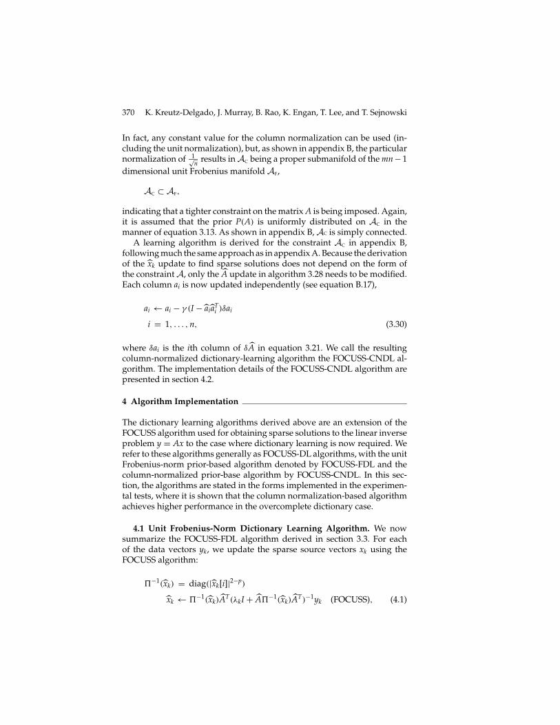
where δai is the ith column of δA in equation 3.21. We call the resultingcolumn-normalized dictionary-learning algorithm the FOCUSS-CNDL al-gorithm. The implementation details of the FOCUSS-CNDL algorithm arepresented in section 4.2.
4 Algorithm Implementation
The dictionary learning algorithms derived above are an extension of theFOCUSS algorithm used for obtaining sparse solutions to the linear inverseproblem y = Ax to the case where dictionary learning is now required. Werefer to these algorithms generally as FOCUSS-DL algorithms, with the unitFrobenius-norm prior-based algorithm denoted by FOCUSS-FDL and thecolumn-normalized prior-base algorithm by FOCUSS-CNDL. In this sec-tion, the algorithms are stated in the forms implemented in the experimen-tal tests, where it is shown that the column normalization-based algorithmachieves higher performance in the overcomplete dictionary case.
4.1 Unit Frobenius-Norm Dictionary Learning Algorithm. We nowsummarize the FOCUSS-FDL algorithm derived in section 3.3. For eachof the data vectors yk, we update the sparse source vectors xk using theFOCUSS algorithm:
�−1(xk) = diag(|xk[i]|2−p)
xk ← �−1(xk)AT(λkI + A�−1(xk)AT)−1yk (FOCUSS), (4.1)
Dictionary Learning Algorithms for Sparse Representation 371
where λk = β(xk) is the regularization parameter. After updating the Nsource vectors xk, k = 1, . . . , n, the dictionary A is reestimated,
�yx =1N
N∑k=1
ykxTk
�xx =1N
N∑k=1
xkxTk
δA = A�xx −�yx
A ← A− γ (δA− tr(ATδA)A), γ > 0, (4.2)
where γ controls the learning rate. For the experiments in section 5, the datablock size is N = 100. During each iteration all training vectors are updatedusing equation 4.1, with a corresponding number of dictionary updatesusing equation 4.2. After each update of the dictionary A, it is renormalizedto have unit Frobenius norm, ‖A‖F = 1.
The learning algorithm is a combined iteration, meaning that the FOCUSSalgorithm is allowed to run for only one iteration (not until full convergence)before the A update step. This means that during early iterations, the xk arein general not sparse. To facilitate learning A, the covariances �yx and �xxare calculated with sparsified xk that have all but the r largest elements setto zero. The value of r is usually set to the largest desired number of nonzeroelements, but this choice does not appear to be critical.
The regularization parameter λk is taken to be a monotonically increasingfunction of the iteration number,
λk = λmax tanh(10−3 · (iter− 1500))+ 1). (4.3)
While this choice of λk does not have the optimality properties of the modi-fied L-curve method (see section 2.5), it does not require a one-dimensionaloptimization for each xk and so is much less computationally expensive.This is further discussed below.
4.2 Column Normalized Dictionary Learning Algorithm. The im-proved version of the algorithm called FOCUSS-CNDL, which providesincreased accuracy especially in the overcomplete case, was proposed inMurray and Kreutz-Delgado (2001). The three key improvements are col-umn normalization that restricts the learned A, an efficient way of adjustingthe regularization parameter λk, and reinitialization to escape from local op-tima.
The column-normalized learning algorithm discussed in section 3.4 andderived in appendix B is used. Because the xk update does not dependon the constraint set A, the FOCUSS algorithm in equation 4.1 is used to
372 K. Kreutz-Delgado, J. Murray, B. Rao, K. Engan, T. Lee, and T. Sejnowski
update N vectors, as discussed in section 4.1. After every N source vectorsare updated, each column of the dictionary is then updated as
ai ← ai − γ (I − aiaTi )δai
i = 1, . . . , n, (4.4)
where δai are the columns of δA, which is found using equation 4.2. Afterupdating each ai, it is renormalized to ‖ai‖2 = 1/n by
ai ← ai√n‖ai‖
, (4.5)
which also ensures that ‖A‖F = 1 as shown in section B.1.The regularization parameter λk may be set independently for each vec-
tor in the training set, and a number of methods have been suggested,including quality of fit (which requires a certain level of reconstruction ac-curacy), sparsity (requiring a certain number of nonzero elements), andthe L-curve which attempts to find an optimal trade-off (Engan, 2000). TheL-curve method works well, but it requires solving a one-dimensional op-timization for each λk, which becomes computationally expensive for largeproblems. Alternatively, we use a heuristic method that allows the trade-offbetween error and sparsity to be tuned for each application, while lettingeach training vector yk have its own regularization parameter λk to improvethe quality of the solution,
λk = λmax
(1− ‖yk − Axk‖
‖yk‖
), λk, λmax > 0. (4.6)
For data vectors that are represented accurately, λk will be large, driving thealgorithm to find sparser solutions. If the SNR can be estimated, we can setλmax = (SNR)−1.
The optimization problem, 3.15, is concave when p ≤ 1, so there willbe multiple local minima. The FOCUSS algorithm is guaranteed to con-verge only to one of these local minima, but in some cases, it is possible todetermine when that has happened by noticing if the sparsity is too low. Pe-riodically (after a large number of iterations), the sparsity of the solutions xkis checked, and if found too low, xk is reinitialized randomly. The algorithmis also sensitive to initial conditions, and prior information may be incor-porated into the initialization to help convergence to the global solution.
5 Experimental Results
Experiments were performed using complete dictionaries (n = m) and over-complete dictionaries (n > m) on both synthetically generated data and
Dictionary Learning Algorithms for Sparse Representation 373
natural images. Performance was measured in a number of ways. With syn-thetic data, performance measures include the SNR of the recovered sourcesxk compared to the true generating source and comparing the learned dic-tionary with the true dictionary. For images of natural scenes, the true un-derlying sources are not known, so the accuracy and efficiency of the imagecoding are found.
5.1 Complete Dictionaries: Comparison with ICA. To test the FOCUSS-FDL and FOCUSS-CNDL algorithms, simulated data were created follow-ing the method of Engan et al. (1999) and Engan (2000). The dictionary A ofsize 20×20 was created by drawing each element aij from a normal distribu-tion with µ = 0, σ 2 = 1 (written as N (0, 1)) followed by a normalization toensure that ‖A‖F = 1. Sparse source vectors xk, k = 1, . . . , 1000 were createdwith r = 4 nonzero elements, where the r nonzero locations are selectedat random (uniformly) from the 20 possible locations. The magnitudes ofeach nonzero element were also drawn from N (0, 1) and limited so that|xkl| > 0.1. The input data yk were generated using y = Ax (no noise wasadded).
For the first iteration of the algorithm, the columns of the initializa-tion estimate, Ainit, were taken to be the first n = 20 training vectors yk.The initial xk estimates were then set to the pseudoinverse solution xk =AT
init(AinitATinit)
−1yk. The constant parameters of the algorithm were set asfollows: p = 1.0, γ = 1.0, and λmax = 2 × 10⁻³ (low noise, assumed SNR≈ 27 dB). The algorithms were run for 200 iterations through the entiredata set, and during each iteration, A was updated after updating 100 datavectors xk.
To measure performance, the SNR between the recovered sources xk andthe the true sources xk were calculated. Each element xk[i] for fixed i wasconsidered as a time-series vector with 1000 elements, and SNRi for eachwas found using
SNRi = 10 log10
( ‖xk[i]‖2
‖xk[i]− xk[i]‖2
). (5.1)
The final SNR is found by averaging SNRi over the i = 1, . . . , 20 vectorsand 20 trials of the algorithms. Because the dictionary A is learned only towithin a scaling factor and column permutations, the learned sources mustbe matched with corresponding true sources and scaled to unit norm beforethe SNR calculation is done.
The FOCUSS-FDL and FOCUSS-CNDL algorithms were compared withextended ICA (Lee, Girolami, & Sejnowski, 1999) and Fastica8 (Hyvarinen
8 Matlab and C versions of extended ICA can be found on-line at http://www.cnl.salk.edu/∼tewon/ICA/code.html. Matlab code for FastICA can be found at: http://www.cis.hut.fi/projects/ica/fastica/.
374 K. Kreutz-Delgado, J. Murray, B. Rao, K. Engan, T. Lee, and T. Sejnowski
15.0 18.0 21.0 24.0 27.0 30.0
Fast ICA
Extended ICA
FOCUSS-FDL
FOCUSS-CNDL
Signal-to-noise ratio (SNR) of recovered sources
SNR (dB) (+/- std dev)
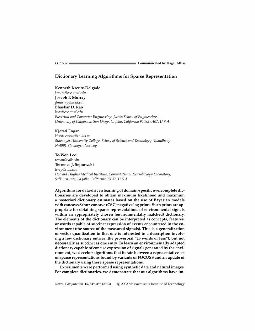
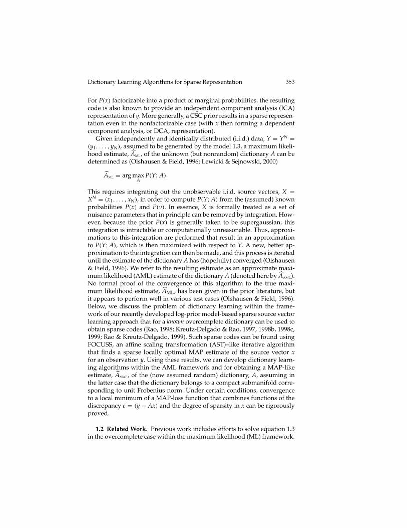
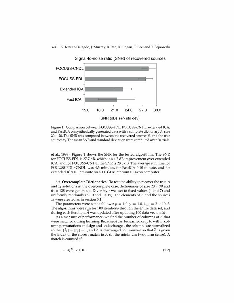
Figure 1: Comparison between FOCUSS-FDL, FOCUSS-CNDL, extended ICA,and FastICA on synthetically generated data with a complete dictionary A, size20× 20. The SNR was computed between the recovered sources xk and the truesources xk. The mean SNR and standard deviation were computed over 20 trials.
et al., 1999). Figure 1 shows the SNR for the tested algorithms. The SNRfor FOCUSS-FDL is 27.7 dB, which is a 4.7 dB improvement over extendedICA, and for FOCUSS-CNDL, the SNR is 28.3 dB. The average run time forFOCUSS-FDL/CNDL was 4.3 minutes, for FastICA 0.10 minute, and forextended ICA 0.19 minute on a 1.0 GHz Pentium III Xeon computer.
5.2 Overcomplete Dictionaries. To test the ability to recover the true Aand xk solutions in the overcomplete case, dictionaries of size 20 × 30 and64 × 128 were generated. Diversity r was set to fixed values (4 and 7) anduniformly randomly (5–10 and 10–15). The elements of A and the sourcesxk were created as in section 5.1.
The parameters were set as follows: p = 1.0, γ = 1.0, λmax = 2 × 10⁻³.The algorithms were run for 500 iterations through the entire data set, andduring each iteration, A was updated after updating 100 data vectors xk.
As a measure of performance, we find the number of columns of A thatwere matched during learning. Because A can be learned only to within col-umn permutations and sign and scale changes, the columns are normalizedso that ‖ai‖ = ‖aj‖ = 1, and A is rearranged columnwise so that aj is giventhe index of the closest match in A (in the minimum two-norm sense). Amatch is counted if
1− |aTi ai| < 0.01. (5.2)
Dictionary Learning Algorithms for Sparse Representation 375
Table 1: Synthetic Data Results.
Learned A Columns Learned x
Algorithm Size of A Diversity, r Average SD % Average SD %
FOCUSS-FDL 20× 30 7 25.3 3.4 84.2 675.9 141.0 67.6FOCUSS-CNDL 20× 30 7 28.9 1.6 96.2 846.8 97.6 84.7FOCUSS-CNDL 64× 128 7 125.3 2.1 97.9 9414.0 406.5 94.1FOCUSS-CNDL 64× 128 5–10 126.3 1.3 98.6 9505.5 263.8 95.1FOCUSS-FDL 64× 128 10–15 102.8 4.5 80.3 4009.6 499.6 40.1FOCUSS-CNDL 64× 128 10–15 127.4 1.3 99.5 9463.4 330.3 94.6
Similarly, the number of matching xk are counted (after rearranging theelements in accordance with the indices of the rearranged A),
1− |xTi xi| < 0.05. (5.3)
If the data are generated by an A that is not column normalized, othermeasures of performance need to be used to compare xk and xk.
The performance is summarized in Table 1, which compares the FOCUSS-FDL with the column-normalized algorithm (FOCUSS-CNDL). For the 20×30 dictionary, 1000 training vectors were used, and for the 64×128 dictionary10,000 were used. Results are averaged over four or more trials. For the64 × 128 matrix and r = 10–15, FOCUSS-CNDL is able to recover 99.5%(127.4/128) of the columns of A and 94.6% (9463/10,000) of the solutions xkto within the tolerance given above. This shows a clear improvement overFOCUSS-FDL, which learns only 80.3% of the A columns and 40.1% of thesolutions xk.
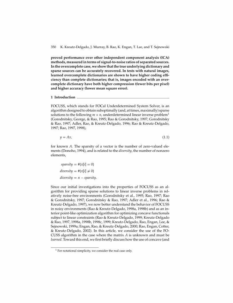
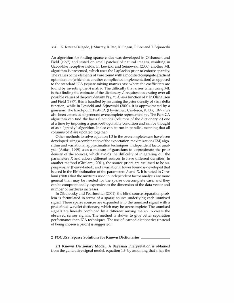
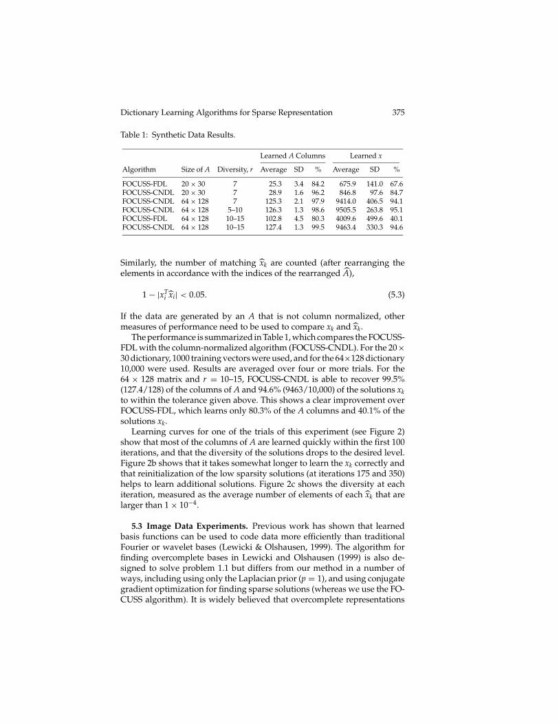
Learning curves for one of the trials of this experiment (see Figure 2)show that most of the columns of A are learned quickly within the first 100iterations, and that the diversity of the solutions drops to the desired level.Figure 2b shows that it takes somewhat longer to learn the xk correctly andthat reinitialization of the low sparsity solutions (at iterations 175 and 350)helps to learn additional solutions. Figure 2c shows the diversity at eachiteration, measured as the average number of elements of each xk that arelarger than 1× 10⁻⁴.
5.3 Image Data Experiments. Previous work has shown that learnedbasis functions can be used to code data more efficiently than traditionalFourier or wavelet bases (Lewicki & Olshausen, 1999). The algorithm forfinding overcomplete bases in Lewicki and Olshausen (1999) is also de-signed to solve problem 1.1 but differs from our method in a number ofways, including using only the Laplacian prior (p = 1), and using conjugategradient optimization for finding sparse solutions (whereas we use the FO-CUSS algorithm). It is widely believed that overcomplete representations
376 K. Kreutz-Delgado, J. Murray, B. Rao, K. Engan, T. Lee, and T. Sejnowski
0 100 200 300 400 5000
50
100
(C) Average diversity (n sparsity) = 13.4
Non
zero
ele
men
ts o
f x
Iteration
0 100 200 300 400 5000
50
100
(A) Matching columns in A = 128
Num
ber
mat
chin
g
0 100 200 300 400 5000
2000
4000
6000
8000
10000
(B) Matching solutions xk = 9573
Iteration
Num
ber
mat
chin
g
Iteration
Figure 2: Performance of the FOCUSS-CNDL algorithm with overcomplete dic-tionary A, size 64 × 128. (a) Number of correctly learned columns of A at eachiteration. (b) Number of sources xk learned. (c) Average diversity (n-sparsity) ofthe xk. The spikes in b and c indicate where some solutions xk were reinitializedbecause they were not sparse enough.
Dictionary Learning Algorithms for Sparse Representation 377
are more efficient than complete bases, but in Lewicki and Olshausen (1999),the overcomplete code was less efficient for image data (measured in bitsper pixel entropy), and it was suggested that different priors could be usedto improve the efficiency. Here, we show that our algorithm is able to learnmore efficient overcomplete codes for priors with p < 1.
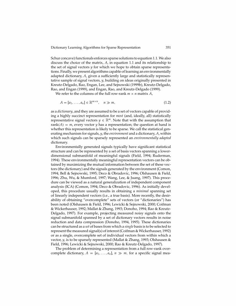
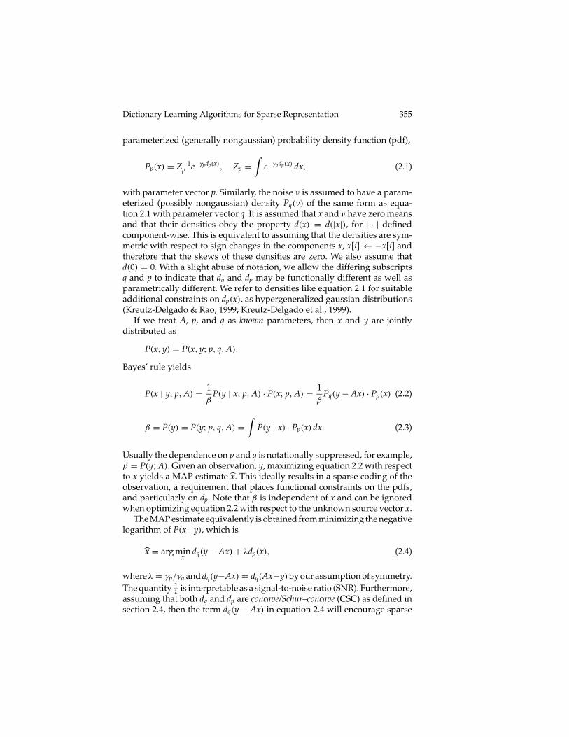
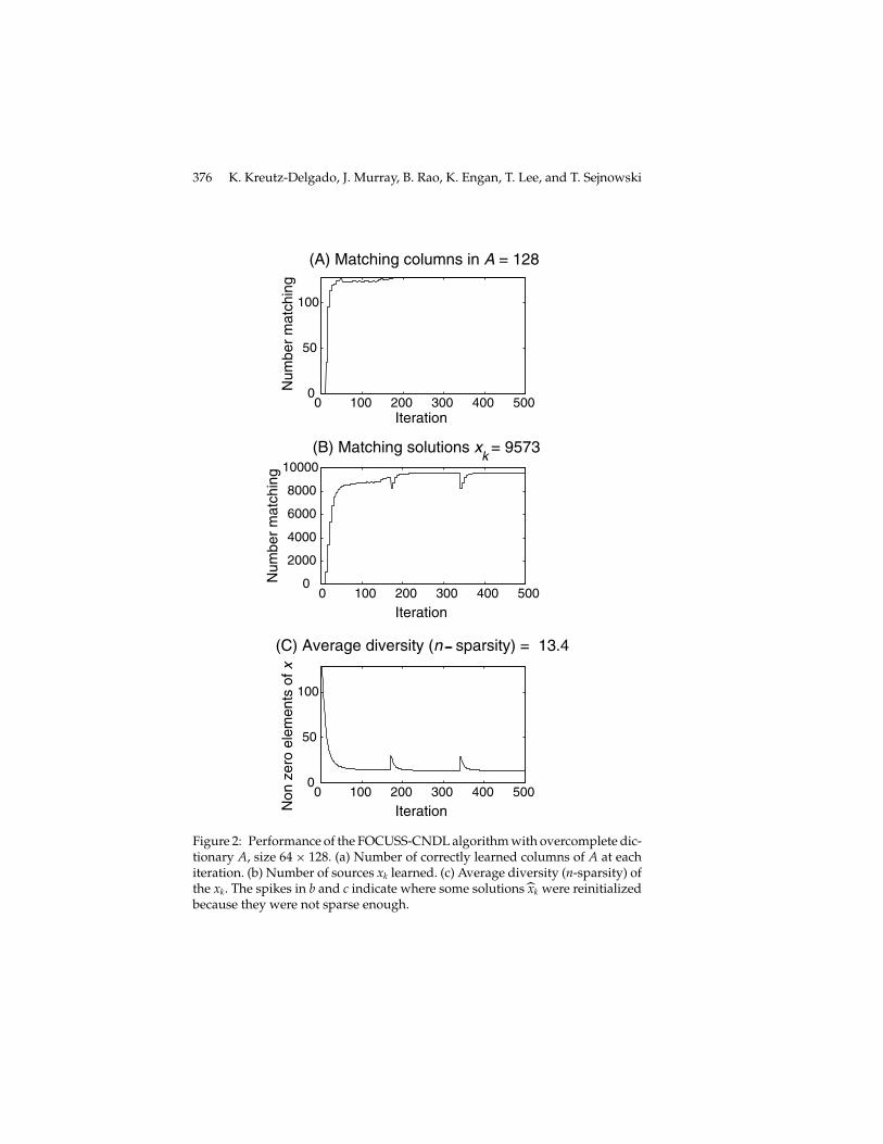
The training data consisted of 10,000 8 × 8 image patches drawn atrandom from black and white images of natural scenes. The parameterp was varied from 0.5–1.0, and the FOCUSS-CNDL algorithm was trainedfor 150 iterations. The complete dictionary (64 × 64) was compared withthe 2× overcomplete dictionary (64 × 128). Other parameters were set:γ = 0.01, λmax = 2 × 10⁻³. The coding efficiency was measured usingthe entropy (bits per pixel) method described in Lewicki and Olshausen(1999). Figure 3 plots the entropy versus reconstruction error (root meansquare error, RMSE) and shows that when p < 0.9, the entropy is less forthe overcomplete representation at the same RMSE.
An example of coding an entire image is shown in Figure 4. The originaltest image (see Figure 4a) of size 256× 256 was encoded using the learneddictionaries. Patches from the test image were not used during training. Ta-ble 2 gives results for low- and high-compression cases. In both cases, codingwith the overcomplete dictionary (64×128) gives higher compression (lowerbits per pixel) and lower error (RMSE). For the high-compression case (see
2 2.5 3 3.5 4 4.50.10
0.15
0.20
0.25
0.30
Comparison of image coding efficiency
Entropy (bits/pixel)
Rec
onst
ruct
ion
erro
r (R
MS
E)
64x64 complete 64x128 overcomplete
Figure 3: Comparing the coding efficiency of complete and 2× overcompleterepresentations on 8×8 pixel patches drawn from natural images. The points onthe curve are the results from different values of p, at the bottom right, p = 1.0,and at the top left, p = 0.5. For smaller p, the overcomplete case is more efficientat the same level of reconstruction error (RMSE).
378 K. Kreutz-Delgado, J. Murray, B. Rao, K. Engan, T. Lee, and T. Sejnowski
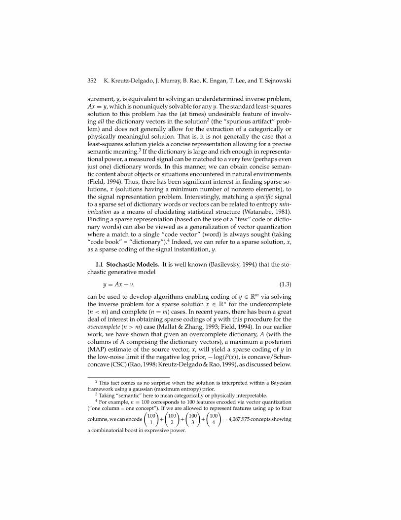
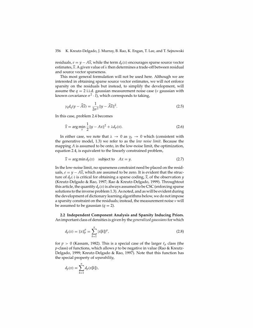
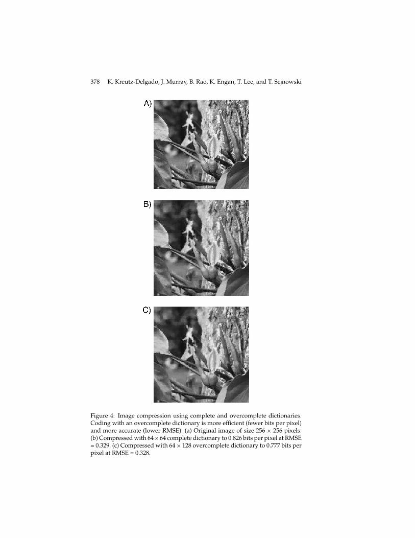
Figure 4: Image compression using complete and overcomplete dictionaries.Coding with an overcomplete dictionary is more efficient (fewer bits per pixel)and more accurate (lower RMSE). (a) Original image of size 256 × 256 pixels.(b) Compressed with 64×64 complete dictionary to 0.826 bits per pixel at RMSE= 0.329. (c) Compressed with 64× 128 overcomplete dictionary to 0.777 bits perpixel at RMSE = 0.328.
Dictionary Learning Algorithms for Sparse Representation 379
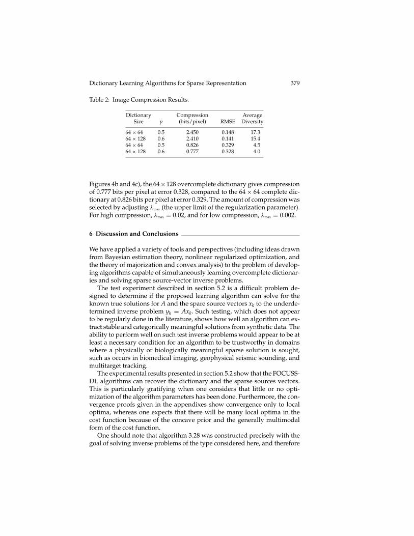
Table 2: Image Compression Results.
Dictionary Compression AverageSize p (bits/pixel) RMSE Diversity
64× 64 0.5 2.450 0.148 17.364× 128 0.6 2.410 0.141 15.464× 64 0.5 0.826 0.329 4.564× 128 0.6 0.777 0.328 4.0
Figures 4b and 4c), the 64×128 overcomplete dictionary gives compressionof 0.777 bits per pixel at error 0.328, compared to the 64× 64 complete dic-tionary at 0.826 bits per pixel at error 0.329. The amount of compression wasselected by adjusting λmax (the upper limit of the regularization parameter).For high compression, λmax = 0.02, and for low compression, λmax = 0.002.
6 Discussion and Conclusions
We have applied a variety of tools and perspectives (including ideas drawnfrom Bayesian estimation theory, nonlinear regularized optimization, andthe theory of majorization and convex analysis) to the problem of develop-ing algorithms capable of simultaneously learning overcomplete dictionar-ies and solving sparse source-vector inverse problems.
The test experiment described in section 5.2 is a difficult problem de-signed to determine if the proposed learning algorithm can solve for theknown true solutions for A and the spare source vectors xk to the underde-termined inverse problem yk = Axk. Such testing, which does not appearto be regularly done in the literature, shows how well an algorithm can ex-tract stable and categorically meaningful solutions from synthetic data. Theability to perform well on such test inverse problems would appear to be atleast a necessary condition for an algorithm to be trustworthy in domainswhere a physically or biologically meaningful sparse solution is sought,such as occurs in biomedical imaging, geophysical seismic sounding, andmultitarget tracking.
The experimental results presented in section 5.2 show that the FOCUSS-DL algorithms can recover the dictionary and the sparse sources vectors.This is particularly gratifying when one considers that little or no opti-mization of the algorithm parameters has been done. Furthermore, the con-vergence proofs given in the appendixes show convergence only to localoptima, whereas one expects that there will be many local optima in thecost function because of the concave prior and the generally multimodalform of the cost function.
One should note that algorithm 3.28 was constructed precisely with thegoal of solving inverse problems of the type considered here, and therefore
380 K. Kreutz-Delgado, J. Murray, B. Rao, K. Engan, T. Lee, and T. Sejnowski
one must be careful when comparing the results given here with other al-gorithms reported in the literature. For instance, the mixture-of-gaussiansprior used in Attias (1999) does not necessarily enforce sparsity. While otheralgorithms in the literature might perform well on this test experiment, tothe best of our knowledge, possible comparably performing algorithmssuch as Attias (1999), Girolami (2001), Hyvarinen et al. (1999), and Lewickiand Olshausen (1999) have not been tested on large, overcomplete matricesto determine their accuracy in recovering A, and so any comparison alongthese lines would be premature. In section 5.1, the FOCUSS-DL algorithmswere compared to the well-known extended ICA and FastICA algorithmsin a more conventional test with complete dictionaries. Performance wasmeasured in terms of the accuracy (SNR) of the recovered sources xk, andboth FOCUSS-DL algorithms were found to have significantly better per-formance (albeit with longer run times).
We have also shown that the FOCUSS-CNDL algorithm can learn an over-complete representation, which can encode natural images more efficientlythan complete bases learned from data (which in turn are more efficient thanstandard nonadaptive bases, such as Fourier or wavelet bases; Lewicki &Olshausen, 1999). Studies of the human visual cortex have shown a higherdegree of overrepresentation of the fovea compared to the other mammals,which suggests an interesting connection between overcomplete represen-tations and visual acuity and recognition abilities (Popovic & Sjostrand,2001).
Because the coupled dictionary learning and sparse-inverse solving al-gorithms are merged and run in parallel, it should be possible to run thealgorithms in real time to track dictionary evolution in quasistationary en-vironments once the algorithm has essentially converged. One way to dothis would be to constantly present randomly encountered new signals, yk,to the algorithm at each iteration instead of the original training set. Onealso has to ensure that the dictionary learning algorithm is sensitive to thenew data so that dictionary tracking can occur. This would be done by anappropriate adaptive filtering of the current dictionary estimate driven bythe new-data derived corrections, similar to techniques used in the adaptivefiltering literature (Kalouptsidis & Theodoridis, 1993).
Appendix A: The Frobenius-Normalized Prior Learning Algorithm
Here we provide a derivation of the algorithm 3.20–3.21 and prove thatit converges to a local minimum of equation 3.15 on the manifold AF ={A | ‖A‖F = 1} ⊂ R
m×n defined in equation 3.17. Although we focus on thedevelopment of the learning algorithm onAF, the derivations in sections A.2and A.3, and the beginning of subsection are done for a general constraintmanifold A.
Dictionary Learning Algorithms for Sparse Representation 381
A.1 Admissible Matrix Derivatives.
A.1.1 The Constraint Manifold AF. In order to determine the structuralform of admissible derivatives, A = d
dt A for matrices belonging to AF,9 it isuseful to view AF as embedded in the finite-dimensional Hilbert space ofmatrices, R
m×n, with inner product
〈A, B〉 = tr(ATB) = tr(BTA) = tr(ABT) = tr(BAT).
The corresponding matrix norm is the Frobenius norm,
‖A‖ = ‖A‖F =√
tr ATA =√
tr AAT.
We will call this space the Frobenius space and the associated inner productthe Frobenius inner product. It is useful to note the isometry,
A ∈ Rm×n ⇐⇒ A = vec(A) ∈ R
mn,
where A is the mn-vector formed by stacking the columns of A. Henceforth,bold type represents the stacked version of a matrix (e.g., B = vec(B)). Thestacked vector A belongs to the standard Hilbert space R
mn, which we shallhenceforth refer to as the stacked space. This space has the standard Euclideaninner product and norm,
〈A, B〉 = ATB, ‖A‖ =√
ATA.
It is straightforward to show that
〈A, B〉 = 〈A, B〉 and ‖A‖ = ‖A‖.In particular, we have
A ∈ AF ⇐⇒ ‖A‖ = ‖A‖ = 1.
Thus, the manifold in equation 3.17 corresponds to the (mn−1)–dimensionalunit sphere in the stacked space, Rmn (which, with a slight abuse of notation,we will continue to denote by AF). It is evident that AF is simply connectedso that a path exists between any two elements of AF and, in particular, apath exists between any initial value for a dictionary, Ainit ∈ AF, used toinitialize a learning algorithm, and a desired target value, Afinal ∈ AF.10
9 Equivalently, we want to determine the structure of elements A of the tangent space,TAF, to the smooth manifold AF at the point A.
10 For example, for 0 ≤ t ≤ 1, take the t–parameterized path,
A(t) = (1− t)Ainit + tAfinal
‖(1− t)Ainit + tAfinal‖ .
382 K. Kreutz-Delgado, J. Murray, B. Rao, K. Engan, T. Lee, and T. Sejnowski
A.1.2 Derivatives on AF: The Tangent Space TAF. Determining the formof admissible derivatives on equation 3.17 is equivalent to determining theform of admissible derivatives on the unit R
mn–sphere. On the unit sphere,we have the well-known fact that
A ∈ AF '⇒ ddt‖A‖2 = 2ATA = 0 '⇒ A ⊥ A.
This shows that the general form of A is A = ΛQ, where Q is arbitrary and
Λ =(
I− AAT
‖A‖2
)= (I−AAT) (A.1)
is the stacked space projection operator onto the tangent space of the unitR
mn–sphere at the point A (note that we used the fact that ‖A‖ = 1). The pro-jection operator Λ is necessarily idempotent, Λ = Λ2. Λ is also self-adjoint,Λ = Λ∗, where the adjoint operator Λ∗ is defined by the requirement that
〈Λ∗Q1, Q2〉 = 〈Q1,ΛQ2〉, for all Q1, Q2 ∈ Rmn,
showing that Λ is an orthogonal projection operator. In this case, Λ∗ = ΛT,so that self-adjointness corresponds to Λ being symmetric. One can readilyshow that an idempotent, self-adjoint operator is nonnegative, which in thiscase corresponds to the symmetric, idempotent operator Λ being a positivesemidefinite matrix.
This projection can be easily rewritten in the Frobenius space,
A = ΛQ = Q− 〈A, Q〉A ⇐⇒ A = �Q = Q− 〈A, Q〉A= Q− tr(ATQ)A. (A.2)
Of course, this result can be derived directly in the Frobenius space usingthe fact that
A ∈ AF '⇒ ddt‖A‖2 = 2〈A, A〉 = 2 tr(ATA) = 0,
from which it is directly evident that
A ∈ TAF at A ∈ AF ⇔ 〈A, A〉 = tr ATA = 0, (A.3)
and therefore A must be of the form11
A = �Q = Q− tr(ATQ)
tr(ATA)A = Q− tr(ATQ)A. (A.4)
11 It must be the case that � = I − |A〉〈A|‖A‖2 = I − |A〉〈A|, using the physicist’s “bra-ket”
notation (Dirac, 1958).
Dictionary Learning Algorithms for Sparse Representation 383
One can verify that � is idempotent and self-adjoint and is therefore anonnegative, orthogonal projection operator. It is the orthogonal projectionoperator from R
m×n onto the tangent space TAF.In the stacked space (with some additional abuse of notation), we repre-
sent the quadratic form for positive semidefinite symmetric matrices W as
‖A‖2W = ATWA.
Note that this defines a weighted norm if, and only if, W is positive defi-nite, which might not be the case by definition. In particular, when W = Λ,the quadratic form ‖A‖2
Λis only positive semidefinite. Finally, note from
equation A.4 that ∀A ∈ AF,
�Q = 0 ⇐⇒ Q = cA, with c = tr(ATQ). (A.5)
A.2 Minimizing the Loss Function over a General Manifold A. Con-sider the Lyapunov function,
VN(X, A) = 〈dq(y− Ax)+ λdp(x)〉N, A ∈ A, (A.6)
where A is some arbitrary but otherwise appropriately defined constraintmanifold associated with the prior, equation 3.13. Note that this is pre-cisely the loss function to be minimized in equation 3.15. If we can de-termine smooth parameter trajectories (i.e., a parameter-vector adaptationrule) (X, A) such that along these trajectories V(X, A) ≤ 0, then as a conse-quence of the La Salle invariance principle (Khalil, 1996), the parameter val-ues will converge to the largest invariant set (of the adaptation rule viewedas a nonlinear dynamical system) contained in the set
� = {(X, A) | VN(X, A) ≡ 0 and A ∈ A}. (A.7)
The set � contains the local minima of VN. With some additional technicalassumptions (generally dependent on the choice of adaptation rule), theelements of � will contain only local minima of VN.
Assuming the i.i.d. q = 2 gaussian measurement noise case of equa-tion 3.8,12 the loss (Lyapunov) function to be minimized is then
VN(X, A) =⟨
12‖Ax− y‖2 + λdp(x)
⟩N
, A ∈ A, (A.8)
which is essentially the loss function to be minimized in equation 3.15.13
12 Note that in the appendix, unlike the notation used in equations 3.8 et seq., the “hat”notation has been dropped. Nonetheless, it should be understood that the quantities Aand X are unknown parameters to be optimized over in equation 3.15, while the measuredsignal vectors Y are known.
13 The factor 12 is added for notational convenience and does not materially affect the
derivation.
384 K. Kreutz-Delgado, J. Murray, B. Rao, K. Engan, T. Lee, and T. Sejnowski
Suppose for the moment, as in equations 3.4 through 3.9, that X is as-sumed to be known, and note that then (ignoring constant terms dependingon X and Y) VN can be rewritten as
VN(A) = 〈tr(Ax− y)(Ax− y)T〉N= 〈tr(AxxTAT)− 2 tr(AxyT)+ tr(yyT)〉N= tr A�xxAT − 2 tr A�xy
VN(A) = tr{A�xxAT − 2A�xy},
for �xx and �xy = �Tyx defined as in equation 3.10. Using standard results
from matrix calculus (Dhrymes, 1984), we can show that VN(A) is minimizedby the solution 3.9. This is done by setting
∂
∂AVN(A) = 0,
and using the identities (valid for W symmetric)
∂
∂Atr AWAT = 2AW and
∂
∂Atr AB = BT.
This yields (assuming that �xx is invertible),
∂
∂AVN(A) = 2A�xx − 2�T
xy = 2(A�xx −�yx) = 0,
⇒ A = �yx�−1xx ,
which is equation 3.9, as claimed. For �xx nonsingular, the solution is uniqueand globally optimal. This is, of course, a well-known result.
Now return to the general case, equation A.8, where both X and A areunknown. For the data indexed by k = 1, . . . , N, define the quantities
dk = dp(xk), e(x) = Ax− y, and ek = Axk − yk.
The loss function and its time derivative can be written,
VN(X, A) =⟨
12
eT(x)e(x)+ λdp(x)
⟩N
VN(X, A) = 〈eT(x)e(x)+ λ∇Tdp(x)x〉N= 〈eT(x)(Ax+ Ax)+ λ∇Tdp(x)x〉N.
Then, to determine an appropriate adaptation rule, note that
VN = T1 + T2, (A.9)
Dictionary Learning Algorithms for Sparse Representation 385
where
T1 = 〈(eT(x)A+ λ∇Tdp(x))x〉N = 1N
N∑k=1
(eTk A+ λ∇Tdk)xk (A.10)
and
T2 = 〈eT(x)Ax〉N = 1N
N∑k=1
eTk Axk. (A.11)
Enforcing the separate conditions
T1 ≤ 0 and T2 ≤ 0, (A.12)
(as well as the additional condition that A ∈ A) will be sufficient to ensurethat VN ≤ 0 on A. In this case, the solution-containing set � of equation A.7is given by
� = {(X, A) | T1(X, A) ≡ 0, T2(X, A) ≡ 0 and A ∈ A}. (A.13)
Note that if A is known and fixed, then T2 ≡ 0, and only the first conditionof equation A.12 (which enforces learning of the source vectors, xk) is ofconcern. Contrawise, if source vectors xk, which ensure that e(xk) = 0 arefixed and known, then T1 ≡ 0, and the second condition of equation A.12(which enforces learning of the dictionary matrix, A) is at issue.
A.3 Obtaining the xk Solutions with the FOCUSS Algorithm. We nowdevelop the gradient factorization-based derivation of the FOCUSS algo-rithm, which provides estimates of xk while satisfying the first convergencecondition of equation A.12. The constraint manifold A is still assumed tobe arbitrary. To enforce the condition T1 ≤ 0 and derive the first adaptationrule given in equation 3.20, we note that we can factor ∇dk = ∇d(xk) as(Kreutz-Delgado & Rao, 1997; Rao & Kreutz-Delgado, 1999)
∇dk = αk�kxk
with αk = αxk > 0 and �xk = �k positive definite and diagonal for allnonzero xk. Then, defining βk = λαk > 0 and selecting an arbitrary set of(adaptable) symmetric positive-definite matrices �k, we choose the learningrule
xk = −�k{ATek + λ∇dk} = −�k{(ATA+ βk�k)xk − ATyk},k = 1, . . . , N, (A.14)
386 K. Kreutz-Delgado, J. Murray, B. Rao, K. Engan, T. Lee, and T. Sejnowski
which is the adaptation rule for the state estimates xk = xk given in the firstline of equation 3.20. With this choice, we obtain
T1 = −〈‖ATe(x)+ λ∇d(x)‖2�〉N
= − 1N
N∑k=1
‖ATek + λ∇dk‖2�k
= − 1N
N∑k=1
‖(ATA+ βk�k)xk − ATyk‖2�k≤ 0, (A.15)
as desired. Assuming convergence to the set A.13 (which will be seen to bethe case after we show below how to ensure that we also have T2 ≤ 0), wewill asymptotically obtain (reintroducing the “hat” notation to now denoteconverged parameter estimates)
‖(ATA+ βk�k )xk − ATyk‖2�k≡ 0, k = 1, . . . , N,
which is equivalent to
xk = (ATA+ βk�k)−1ATyk, k = 1, . . . , N, (A.16)
at convergence. This is also equivalent to the condition given in the first lineof equation 3.25, as shown below.
Exploiting the fact that �k in equation A.14 are arbitrary (subject to thesymmetry and positive-definiteness constraint), let us make the specificchoice shown in equation 3.23,
�k = ηk(ATA+ βk�k)−1, ηk > 0, k = 1, . . . , N. (A.17)
Also note the (trivial) identity,
(ATA+ β�)�−1AT = AT(A�−1AT + βI),
which can be recast nontrivially as
(ATA+ β�)−1AT = �−1AT(βI + A�−1AT)−1. (A.18)
With equations A.17 and A.18, the learning rule, A.14, can be recast as
xk = −ηk{xk −�−1k AT(βkI + A�−1
k AT)−1yk}, k = 1, . . . , N, (A.19)
which is the alternative learning algorithm, 3.24. At convergence (whenT1 ≡ 0) we have the condition shown in the first line of equation 3.25,
xk = �−1AT(βkI + A�−1AT)−1yk. (A.20)
Dictionary Learning Algorithms for Sparse Representation 387
This also follows from the convergence condition A.16 and the identity A.18,showing that the result, A.20, is independent of the specific choice of �k > 0.Note from equations A.14 and A.15 that T1 ≡ 0 also results in xk ≡ 0 fork = 1, . . . , N, so that we will have converged to constant values, xk, whichsatisfy equation A.20.
For the case of known, fixed A, the learning rule derived here will con-verge to sparse solutions, xk, and when discretized as in section 3.3, yieldsequation 3.27, which is the known dictionary FOCUSS algorithm (Rao &Kreutz-Delgado, 1998a, 1999).
Note that the derivation of the sparse source-vector learning algorithmhere, which enforces the condition T1 ≤ 0, is entirely independent of anyconstraints placed on A (such as, for example, the unit Frobenius-norm andcolumn-norm constraints considered in this article) or of the form of theA-learning rule. Thus alternative choices of constraints placed on A, as con-sidered in Murray and Kreutz-Delgado (2001) and described in appendix B,will not change the form of the xk-learning rule derived here. Of course,because the xk learning rule is strongly coupled to the A-learning rule, algo-rithmic performance and speed of convergence may well be highly sensitiveto conditions placed on A and the specific A learning algorithm used.
A.4 Learning the Dictionary A.
A.4.1 General Results. We now turn to the enforcement of the secondconvergence condition, T2 ≤ 0 and the development of the dictionary adap-tation rule shown in equation 3.20. First, as in equation 3.21, we define theerror term δA as
δA = 〈e(x)xT〉N = 1N
N∑k=1
e(xk)xTk = A�xx −�yx, (A.21)
using the fact that e(x) = Ax− y. Then, from equation A.11, we have
T2 = 〈eT(x)Ax〉N = 〈tr(xeT(x)A)〉N = tr(〈xeT(x)〉NA)
= tr(δATA) = δATA. (A.22)
So far, these steps are independent of any specific constraints that may beplaced on A, other than that the manifold A be smooth and compact. WithA constrained to lie on a specified smooth, compact manifold, to ensurecorrect learning behavior, it is sufficient to impose the constraint that A liesin the tangent space to the manifold and the condition that T2 ≤ 0.
A.4.2 Learning on the Unit Frobenius Sphere, AF. To ensure that T2 ≤ 0and that A is in the tangent space of the unit sphere in the Frobenius spaceR
mn, we take
A=−µΛδA ⇐⇒ A=−µ�δA=−µ(δA− tr(ATδA)A), µ > 0, (A.23)
388 K. Kreutz-Delgado, J. Murray, B. Rao, K. Engan, T. Lee, and T. Sejnowski
which is the adaptation rule given in equation 3.20. With this choice, andusing the positive semidefiniteness of Λ, we have
T2 = −µ‖δA‖2Λ ≤ 0,
as required. Note that at convergence, the condition T2 ≡ 0, yields A ≡ 0, sothat we will have converged to constant values for the dictionary elements,and
0 = �δA = �(A�xx −�yx) '⇒ δA = (A�xx −�yx) = cA, (A.24)
from equation A.5, where c = tr(ATδA). Thus, the steady-state solution is
A = �y,x(�xx − cI)−1 ∈ AF. (A.25)
Note that equations A.20 and A.25 are the steady-state values given earlierin equation 3.25.
Appendix B: Convergence of the Column–Normalized LearningAlgorithm
The derivation and proof of convergence of the column-normalized learn-ing algorithm, applicable to learning members of AC, is accomplished byappropriately modifying key steps of the development given in appendix A.As in appendix A, the standard Euclidean norm and inner product applyto column vectors, while the Frobenius norm and inner product apply tom× n matrix elements of R
m×n.
B.1 Admissible Matrix Derivatives.
B.1.1 The Constraint Manifold AC. Let ei = (0 · · · 0 1 0 · · · 0)T ∈ Rn be
the canonical unit vector whose components are all zero except for the value1 in the ith location. Then
I =n∑
i=1
eieTi and ai = Aei.
Note that
‖ai‖2=aTi ai = (Aei)
TAei = eTi ATAei = tr eieT
i ATA = tr MTi A=〈Mi, A〉,
where
Mi � AeieTi = aieT
i = [0 0 · · · 0 ai 0 · · · 0] ∈ Rm×n. (B.1)
Note that only the ith column of Mi is nonzero and is equal to ai = ithcolumn of A. We therefore have that
A =n∑
i=1
Mi. (B.2)
Dictionary Learning Algorithms for Sparse Representation 389
Also, for i, j = 1, . . . , n,
〈Mi, Mj〉= tr MTi Mj= tr eieT
i ATAejeTj = tr eT
i ATAejeTj ei=‖ai‖2δi,j, (B.3)
where δi,j is the Kronecker delta. Note, in particular, that ‖ai‖ = ‖Mi‖.Let A ∈ AC, where AC is the set of column-normalized matrices, as de-
fined by equation 3.29.AC is an mn−n = n(m−1)–dimensional submanifoldof the Frobenius space R
m×n as each of the n columns of A is normalized as
‖ai‖2 = ‖Mi‖2 ≡ 1n
,
and
‖A‖2 = tr ATA = trn∑
i=1
MTi
n∑j=1
Mj =n∑
i=1
‖ai‖2 = nn= 1,
using linearity of the trace function and property, B.3. It is evident, therefore,that
AC ⊂ AF,
for AF defined by equation 3.17.We can readily show that AC is simply connected, so that a continu-
ous path exists between any matrix A = Ainit ∈ AC to any other column-normalized matrix A′ = AFinal ∈ AC. Indeed, let A and A′ be such that
A = [a1, . . . , an], A′ = [a′1, . . . , a′n],
‖ai‖ = ‖a′j‖ = 1/√
n,∀i, j = 1, . . . , n.
There is obviously a continuous path entirely inAC from A ∈ AC to the inter-mediate matrix [a′1, a2, . . . , an] ∈ AC. Similarly, there is a continuous path en-tirely in AC from [a′1, a2, . . . , an] to [a′1, a′2, . . . , an], and so on to [a′1, . . . , a′n] =A′. To summarize, AC is a simply connected (nm−n)–dimensional subman-ifold of the simply connected (nm− 1)–dimensional manifold AF and theyare both submanifolds of the (nm)–dimensional Frobenius space R
m×n.
B.1.2 Derivatives on AC: The Tangent Space TAC. For convenience, fori = 1, . . . , n define
ai = ai
‖ai‖ =√
nai, ‖ai‖ = 1,
and
Mi = Mi
‖Mi‖ =√
nMi = aieTi , ‖Mi‖ = 1.
390 K. Kreutz-Delgado, J. Murray, B. Rao, K. Engan, T. Lee, and T. Sejnowski
Note that equation B.3 yields
〈Mi, Mj〉 = tr MTi Mj = δi,j. (B.4)
For any A ∈ AC we have for each i = 1, . . . , n,
0 = ddt‖ai‖2 = d
dtaT
i ai = ddt
eTi ATAei = 2eT
i ATAei
= 2 tr eieTi ATA = 2 tr MT
i A,
or
A ∈ AC ⇒ 〈Mi, A〉 = tr MTi A = 0 for i = 1, . . . , n. (B.5)
In fact,
A ∈ TAC at A ∈ AC ⇔ 〈Mi, A〉 = tr MTi A = 0
for i = 1, . . . , n. (B.6)
Note from equations B.2 and B.5 that
〈A, A〉 =⟨
n∑i=1
Mi, A
⟩= 0,
showing that (see equation A.3) TAC ⊂ TAF, as expected from the fact thatAC ⊂ AF.
An important and readily proven fact is that for each i = 1, . . . , n,
tr MTi A = 0 ⇔ A = PiQi (B.7)
for some matrix Qi and projection operator, Pi, defined by
PiQ � Q− Mi〈Mi, Q〉 = Q− Mi tr MTi Q. (B.8)
From equation B.4, it can be shown that the projection operators commute,
PiPj = PjPi, i �= j, i, j = 1, . . . , n, (B.9)
and are idempotent,
P2i = Pi, i = 1, . . . , n. (B.10)
Indeed, it is straightforward to show from equation B.4 that for all Q,
PiPjQ = PjPiQ = Q− Mi〈Mi, Q〉 − Mj〈Mj, Q〉, for all i �= j, (B.11)
Dictionary Learning Algorithms for Sparse Representation 391
and
P2i Q = Q− Mi〈Mi, Q〉 = PiQ, i = 1, . . . , n. (B.12)
It can also be shown that
〈PiQ1, Q2〉 = 〈Q1, PiQ2〉,showing that Pi is self–adjoint, Pi = P∗i .
Define the operator,
P = P1, . . . , Pn. (B.13)
Note that because of the commutativity of the Pi, the order of multiplica-tion on the right-hand side of equation B.11 is immaterial, and it is easilydetermined that P is idempotent,
P2 = P.
By induction on equation B.11, it is readily shown that
PQ = Q−M1〈M1, Q〉−· · ·−Mn〈Mn, Q〉 = Q−n∑
i=1
Mi〈Mi, Q〉. (B.14)
Either from the self-adjointness and idempotency of each Pi, or directly fromequation B.14, it can be shown that P itself is self–adjoint, P = P∗,
〈PQ1, Q2〉 = 〈Q1, PQ2〉.Thus, P is the orthogonal projection operator from R
m×n onto TAC.As a consequence, we have the key result that
A ∈ TAC at A ⇔ A = PQ, (B.15)
for some matrix Q ∈ Rm×n. This follows from the fact that given Q, then
the right-hand side of equation B.6 is true for A = PQ. On the other hand,if the right-hand side of equation B.6 is true for A, we can take Q = Ain equation B.15. Note that for the TAF–projection operator � given byequation A.2, we have that
P = �P = P�,
consistent with the fact that TAC ⊂ TAF.Let qi, i = 1, . . . , n be the columns of Q = [q1, . . . , qn]. The operation
Q′ = PjQ, corresponds to
q′i = qi, i �= j, and q′j = (I − ajaTj )qj,
while the operation Q′ = PQ, corresponds to
q′i = (I − aiaTi )qi, i = 1, . . . , n.
392 K. Kreutz-Delgado, J. Murray, B. Rao, K. Engan, T. Lee, and T. Sejnowski
B.2 Learning on the Manifold AC. The development of equations A.6through A.22 is independent of the precise nature of the constraint manifoldA and can be applied here to the specific case of A = AC. To ensure thatT2 ≤ 0 in equation A.22 and that A ∈ TAC, we can use the learning rule,
A = −µPδA = −µ
(δA−
n∑i=1
Mi tr MiδA
), (B.16)
for µ > 0 and δA given by equation A.21. With the ith column of δA denotedby δai, this corresponds to the learning rule,
ai = −µ(I − aiaTi )δai, i = 1, . . . , n. (B.17)
With rule B.16, we have
T2 = 〈δA, A〉 = −µ〈δA, PδA〉 = −µ〈δA, P2δA〉= −µ〈PδA, PδA〉 = −µ‖PδA‖2 ≤ 0,
where we have explicitly shown that the idempotency and self-adjointnessof P correspond to its being a nonnegative operator. Thus, we will haveconvergence to the largest invariant set for which A ≡ 0, which from equa-tion B.16 is equivalent to the set for which
PδA = δA−n∑
i=1
Mi〈Mi, δA〉 ≡ 0. (B.18)
This, in turn, is equivalent to
δA =n∑
i=1
Mi〈Mi, δA〉 =n∑
i=1
nMi〈Mi, δA〉 =n∑
i=1
ciMi, (B.19)
with
ci � n〈Mi, δA〉 = naTi δai, i = 1, . . . , n.
An equivalent statement to equation B.19 is
δai = ciai, i = 1, . . . , n.
Defining the diagonal matrix
C = diag[ci, . . . , cn]
and recalling the definitions A.21 and B.1, we obtain from equation B.19that
A�xx −�yx = δA = AC,
which can be solved as
A = �yx(�xx − C)−1. (B.20)
This is the general form of the solution found by theAC–learning algorithm.
Dictionary Learning Algorithms for Sparse Representation 393
Acknowledgments
This research was partially supported by NSF grant CCR-9902961. K. K.-D.also acknowledges the support provided by the Computational Neurobiol-ogy Laboratory, Salk Institute, during a 1998–1999 sabbatical visit.
References
Adler, J., Rao, B., & Kreutz-Delgado, K. (1996). Comparison of basis selectionmethods. In Proceedings of the 30th Asilomar Conference on Signals, Systems, andComputers. Pacific Grove, CA: IEEE.
Attias, H. (1999). Independent factor analysis. Neural Computation, 11(4), 803–851.
Basilevsky, A. (1994). Statistical factor analysis and related methods: Theory andapplications. New York: Wiley.
Bell, A., & Sejnowski, T. (1995). An information-maximization approach to blindseparation and blind deconvolution. Neural Computation, 7, 1129–1159.
Coifman, R., & Wickerhauser, M. (1992). Entropy-based algorithms for best basisselection. IEEE Transactions on Information Theory, IT-38(2), 713–718.
Comon, P. (1994). Independent component analysis: A new concept? Signal Pro-cessing, 36, 287–314.
Deco, G., & Obradovic, D. (1996). An information-theoretic approach to neural com-puting. Berlin: Springer-Verlag.
Dhrymes, P. (1984). Mathematics for econometrics (2nd ed.). New York: Springer-Verlag.
Dirac, P. A. M. (1958). The principles of quantum mechanics. Oxford: ClarendonPress.
Donoho, D. (1994). On minimum entropy segmentation. In C. Chui, L. Monte-fusco, & L. Puccio (Eds.), Wavelets: Theory, algorithms, and applications (pp. 233–269). San Diego, CA: Academic Press.
Donoho, D. (1995). De-noising by soft-thresholding. IEEE Trans. on InformationTheory, 41, 613–627.
Engan, K. (2000). Frame based signal representation and compression. Unpublisheddoctoral dissertation, Stavanger Universty College, Norway.
Engan, K., Rao, B., & Kreutz-Delgado, K. (1999). Frame design using FOCUSSwith method of optimal directions (MOD). In Proc. NORSIG-99. Tronheim,Norway: IEEE.
Engan, K., Rao, B. D., & Kreutz-Delgado, K. (2000). Regularized FOCUSS forsubset selection in noise. In Proc. NORSIG 2000, Sweden, June, 2000 (pp. 247–250). Kolmarden, Sweden: IEEE.
Field, D. (1994). What is the goal of sensory coding. Neural Computation, 6, 559–599.
Girolami, M. (2001). A variational method for learning sparse and overcompleterepresentations. Neural Computation, 13, 2517–2532.
Gorodnitsky, I., George, J., & Rao, B. (1995). Neuromagnetic source imagingwith FOCUSS: A recursive weighted minimum norm algorithm. Journal ofElectroencephalography and Clinical Neurophysiology, 95(4), 231–251.
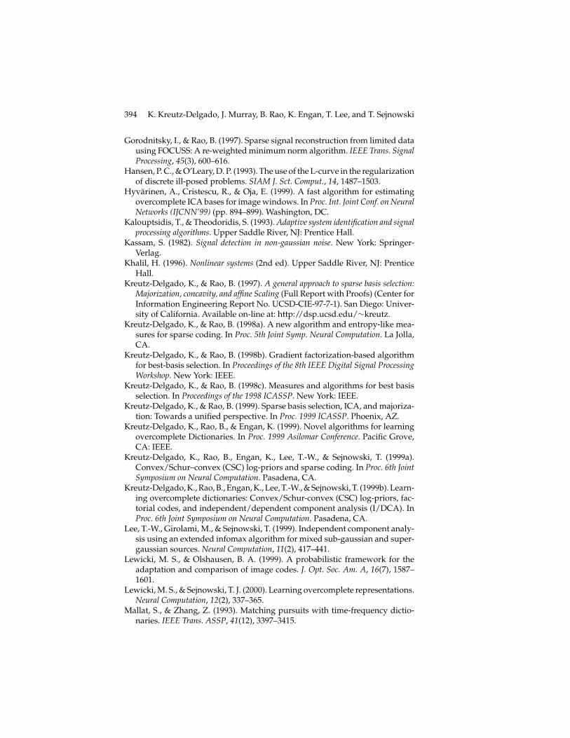
394 K. Kreutz-Delgado, J. Murray, B. Rao, K. Engan, T. Lee, and T. Sejnowski
Gorodnitsky, I., & Rao, B. (1997). Sparse signal reconstruction from limited datausing FOCUSS: A re-weighted minimum norm algorithm. IEEE Trans. SignalProcessing, 45(3), 600–616.
Hansen, P. C., & O’Leary, D. P. (1993). The use of the L-curve in the regularizationof discrete ill-posed problems. SIAM J. Sct. Comput., 14, 1487–1503.
Hyvarinen, A., Cristescu, R., & Oja, E. (1999). A fast algorithm for estimatingovercomplete ICA bases for image windows. In Proc. Int. Joint Conf. on NeuralNetworks (IJCNN’99) (pp. 894–899). Washington, DC.
Kalouptsidis, T., & Theodoridis, S. (1993). Adaptive system identification and signalprocessing algorithms. Upper Saddle River, NJ: Prentice Hall.
Kassam, S. (1982). Signal detection in non-gaussian noise. New York: Springer-Verlag.
Khalil, H. (1996). Nonlinear systems (2nd ed). Upper Saddle River, NJ: PrenticeHall.
Kreutz-Delgado, K., & Rao, B. (1997). A general approach to sparse basis selection:Majorization, concavity, and affine Scaling (Full Report with Proofs) (Center forInformation Engineering Report No. UCSD-CIE-97-7-1). San Diego: Univer-sity of California. Available on-line at: http://dsp.ucsd.edu/∼kreutz.
Kreutz-Delgado, K., & Rao, B. (1998a). A new algorithm and entropy-like mea-sures for sparse coding. In Proc. 5th Joint Symp. Neural Computation. La Jolla,CA.
Kreutz-Delgado, K., & Rao, B. (1998b). Gradient factorization-based algorithmfor best-basis selection. In Proceedings of the 8th IEEE Digital Signal ProcessingWorkshop. New York: IEEE.
Kreutz-Delgado, K., & Rao, B. (1998c). Measures and algorithms for best basisselection. In Proceedings of the 1998 ICASSP. New York: IEEE.
Kreutz-Delgado, K., & Rao, B. (1999). Sparse basis selection, ICA, and majoriza-tion: Towards a unified perspective. In Proc. 1999 ICASSP. Phoenix, AZ.
Kreutz-Delgado, K., Rao, B., & Engan, K. (1999). Novel algorithms for learningovercomplete Dictionaries. In Proc. 1999 Asilomar Conference. Pacific Grove,CA: IEEE.
Kreutz-Delgado, K., Rao, B., Engan, K., Lee, T.-W., & Sejnowski, T. (1999a).Convex/Schur–convex (CSC) log-priors and sparse coding. In Proc. 6th JointSymposium on Neural Computation. Pasadena, CA.
Kreutz-Delgado, K., Rao, B., Engan, K., Lee, T.-W., & Sejnowski, T. (1999b). Learn-ing overcomplete dictionaries: Convex/Schur-convex (CSC) log-priors, fac-torial codes, and independent/dependent component analysis (I/DCA). InProc. 6th Joint Symposium on Neural Computation. Pasadena, CA.
Lee, T.-W., Girolami, M., & Sejnowski, T. (1999). Independent component analy-sis using an extended infomax algorithm for mixed sub-gaussian and super-gaussian sources. Neural Computation, 11(2), 417–441.
Lewicki, M. S., & Olshausen, B. A. (1999). A probabilistic framework for theadaptation and comparison of image codes. J. Opt. Soc. Am. A, 16(7), 1587–1601.
Lewicki, M. S., & Sejnowski, T. J. (2000). Learning overcomplete representations.Neural Computation, 12(2), 337–365.
Mallat, S., & Zhang, Z. (1993). Matching pursuits with time-frequency dictio-naries. IEEE Trans. ASSP, 41(12), 3397–3415.
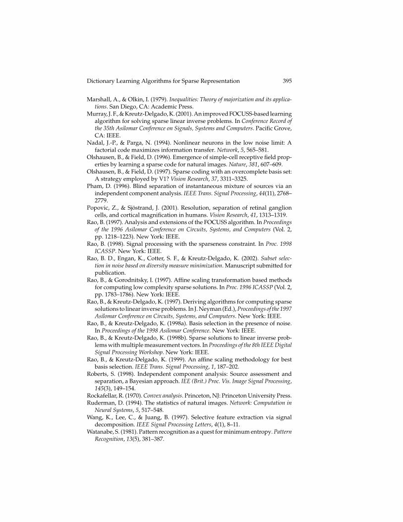
Dictionary Learning Algorithms for Sparse Representation 395
Marshall, A., & Olkin, I. (1979). Inequalities: Theory of majorization and its applica-tions. San Diego, CA: Academic Press.
Murray, J. F., & Kreutz-Delgado, K. (2001). An improved FOCUSS-based learningalgorithm for solving sparse linear inverse problems. In Conference Record ofthe 35th Asilomar Conference on Signals, Systems and Computers. Pacific Grove,CA: IEEE.
Nadal, J.-P., & Parga, N. (1994). Nonlinear neurons in the low noise limit: Afactorial code maximizes information transfer. Network, 5, 565–581.
Olshausen, B., & Field, D. (1996). Emergence of simple-cell receptive field prop-erties by learning a sparse code for natural images. Nature, 381, 607–609.
Olshausen, B., & Field, D. (1997). Sparse coding with an overcomplete basis set:A strategy employed by V1? Vision Research, 37, 3311–3325.
Pham, D. (1996). Blind separation of instantaneous mixture of sources via anindependent component analysis. IEEE Trans. Signal Processing, 44(11), 2768–2779.
Popovic, Z., & Sjostrand, J. (2001). Resolution, separation of retinal ganglioncells, and cortical magnification in humans. Vision Research, 41, 1313–1319.
Rao, B. (1997). Analysis and extensions of the FOCUSS algorithm. In Proceedingsof the 1996 Asilomar Conference on Circuits, Systems, and Computers (Vol. 2,pp. 1218–1223). New York: IEEE.
Rao, B. (1998). Signal processing with the sparseness constraint. In Proc. 1998ICASSP. New York: IEEE.
Rao, B. D., Engan, K., Cotter, S. F., & Kreutz-Delgado, K. (2002). Subset selec-tion in noise based on diversity measure minimization. Manuscript submitted forpublication.
Rao, B., & Gorodnitsky, I. (1997). Affine scaling transformation based methodsfor computing low complexity sparse solutions. In Proc. 1996 ICASSP (Vol. 2,pp. 1783–1786). New York: IEEE.
Rao, B., & Kreutz-Delgado, K. (1997). Deriving algorithms for computing sparsesolutions to linear inverse problems. In J. Neyman (Ed.), Proceedings of the 1997Asilomar Conference on Circuits, Systems, and Computers. New York: IEEE.
Rao, B., & Kreutz-Delgado, K. (1998a). Basis selection in the presence of noise.In Proceedings of the 1998 Asilomar Conference. New York: IEEE.
Rao, B., & Kreutz-Delgado, K. (1998b). Sparse solutions to linear inverse prob-lems with multiple measurement vectors. In Proceedings of the 8th IEEE DigitalSignal Processing Workshop. New York: IEEE.
Rao, B., & Kreutz-Delgado, K. (1999). An affine scaling methodology for bestbasis selection. IEEE Trans. Signal Processing, 1, 187–202.
Roberts, S. (1998). Independent component analysis: Source assessment andseparation, a Bayesian approach. IEE (Brit.) Proc. Vis. Image Signal Processing,145(3), 149–154.
Rockafellar, R. (1970). Convex analysis. Princeton, NJ: Princeton University Press.Ruderman, D. (1994). The statistics of natural images. Network: Computation in
Neural Systems, 5, 517–548.Wang, K., Lee, C., & Juang, B. (1997). Selective feature extraction via signal
decomposition. IEEE Signal Processing Letters, 4(1), 8–11.Watanabe, S. (1981). Pattern recognition as a quest for minimum entropy. Pattern
Recognition, 13(5), 381–387.
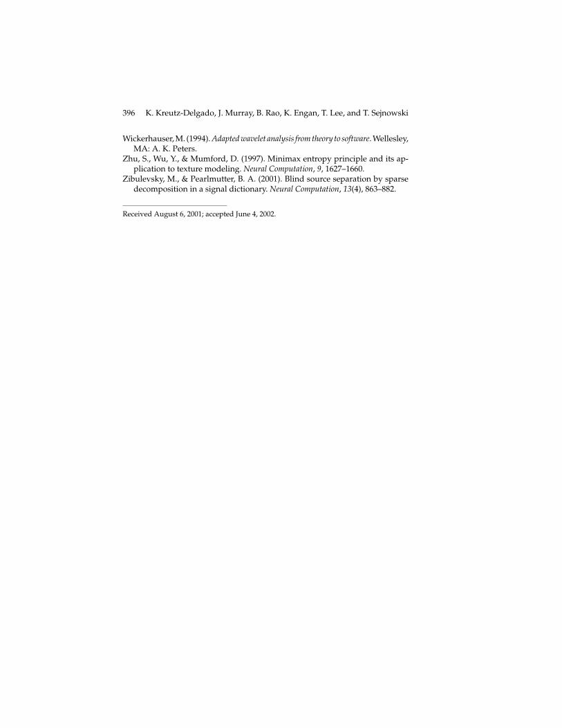
396 K. Kreutz-Delgado, J. Murray, B. Rao, K. Engan, T. Lee, and T. Sejnowski
Wickerhauser, M. (1994). Adapted wavelet analysis from theory to software. Wellesley,MA: A. K. Peters.
Zhu, S., Wu, Y., & Mumford, D. (1997). Minimax entropy principle and its ap-plication to texture modeling. Neural Computation, 9, 1627–1660.
Zibulevsky, M., & Pearlmutter, B. A. (2001). Blind source separation by sparsedecomposition in a signal dictionary. Neural Computation, 13(4), 863–882.
Received August 6, 2001; accepted June 4, 2002.