ANALYSIS OF THE OXYACETYLENE FLAME UNDER DIAMOND

DEPOSITION CONDITIONS USING FOURIER TRANSFORM INFRARED

SPECTROSCOPY

by

ERIC SZETO

Submitted in partial fulfillment of the requirements

for the degree of Master of Science

Thesis Adviser: Dr. Philip W. Morrison Jr.

Department of Chemical Engineering

CASE WESTERN RESERVE UNIVERSITY

January, 1999

ii

ANALYSIS OF THE OXYACETYLENE FLAME UNDER DIAMONDDEPOSITION CONDITIONS USING FOURIER TRANSFORM INFRARED

SPECTROSCOPY

Abstract

by

ERIC SZETO

Diamond has many useful and attractive properties. These applications include

scratchproof coatings, use as a cutting tool, and heat sinks in the microprocessor

industry. Because of its many potential applications, many experiments have been

performed to better understand the chemistry of diamond CVD using a low cost and

high growth rate reactor system: the oxyacetylene torch.

In order to get a better understanding of the chemistry in the oxyacetylene flame

under diamond deposition conditions, Fourier transform infrared spectroscopy along

with the HITRAN database were used to obtain quantitative information on various

species in the flame. Unlike many researchers who have made qualitative or relative

measurements of the species in the flame, this research gave a more quantitative

determination of the species as well as the flame temperature.

The oxyacetylene flame with a total flow rate of 2 slm was analyzed. One of the

important parameters known to influence diamond deposition is the R ratio (flow of

oxygen / flow of acetylene) and the axial distance of the substrate from the tip of the

torch nozzle. Therefore, various R (0.90 to 1.10) and axial positions (0mm to 18mm

from the tip of the nozzle) are analyzed for species concentration. The species

iii

concentrations at the position and R ratio that favors diamond deposition were

compared to unfavorable conditions. In addition, open and enclosed flames were

analyzed and compared since it is reported in literature that the enclosed flame is

better for diamond growth.

iv

ACKNOWLEDGEMENTS

Many people should be acknowledged for their assistance, guidance, help, and

support. First, I acknowledge the guidance and support of Dr. Philip W. Morrison Jr.,

whose efforts are immeasurable. I would also like to acknowledge the American

Chemical Society for their financial support.

I would also like to thank Wayne Schmidt for his help and suggestion for making

and modifying the equipment used for this experiment. Cliff Hayman must be

acknowledged for his help around the lab.

Friends and family gave me tremendous support for this project. Special thanks

goes to Shannon Tsang for her support throughout my project. In addition, I would

like to thank my grandmother for taking care of me when I was young. Most of all, I

would like to thank my mom and dad for giving me the opportunity and support for

my education. Without them, I would have never been able to obtain a college

education.

v

TABLE OF CONTENTS

Page

List of Figures viii

1.0 Introduction 1

1.1 Diamond films and its applications 1

1.2 CVD Methods 1

1.3 The purpose of this work 3

2.0 Prior Research 5

2.1 Open Flames 5

2.2 Enclosed Flames 7

2.3 Diagnostic and Flames 8

2.3.1 Optical Emission Spectroscopy 8

2.3.2 Laser induced fluorescence 8

2.3.3 Absorption spectroscopy 10

2.3.4 Mass spectroscopy 10

2.4 Fourier Transform Infrared Spectroscopy (FTIR) - Background 11

2.5 FTIR Spectroscopy and CVD 14

2.5.1 Emission/transmission measurements 14

2.5.2 FTIR and oxyacetylene flames 16

2.6 HITRAN Database 16

3.0 Equipment Description 23

3.1 Torch Reactor 23

vi

3.2 Spectrometer 23

3.3 Enclosed Flame Apparatus 25

3.4 Operational Procedure 25

4.0 Methods To Eliminate Flame Noise 31

4.1 Problem Statement 31

4.2 Methods to Eliminate Flame Noise 34

4.2.1 Two detector configuration 34

4.2.2 Pointing the flame upward 35

4.2.3 Apertures 37

4.2.4 Blocking the CO and CO2 absorptions 38

4.2.5 Long-pass infrared filters 40

5.0 Analysis of the Open Flame 55

5.1 E/T Temperature Measurements of the Open Flame 55

5.2 CO2 Measurements of the Open Flame 58

5.3 CO Measurements of the Open Flame 59

5.4 H2O Measurements of the Open Flame 60

5.5 OH Measurements of the Open Flame 62

5.6 C2H2 Measurements of the Open Flame 63

5.7 Discussion of Results 64

5.8 Comparison of Results to Previous Work 68

6.0 Analysis of the Enclosed Flame 86

6.1 Equipment Modifications 86

vii

6.1.1 Linear and non-linear detectors 86

6.1.2 Purging the arm of the spectrometer 87

6.2 Temperature Measurements in the Enclosed Flame 88

6.3 CO Measurements in the Enclosed Flame 91

6.4 CO2 Measurements in the Enclosed Flame 92

6.5 H2O Measurements in the Enclosed Flame 92

6.6 OH Measurements in the Enclosed Flame 92

6.7 C2H2 Measurements in the Enclosed Flame 93

6.8 CH4 Measurements in the Enclosed Flame 93

6.9 Discussion of the Enclosed Flame 94

6.10 Oxygen Entrainment in the Enclosed Flame 95

6.11 Comparison of the Free and Enclosed Flame 96

7.0 Conclusion 112

8.0 Future Work 115

Comprehensive References 116

Appendix I 123

viii

LIST OF FIGURES

Page

Figure 1.0-1 Regions of the acetylene flame. 4

Figure 2.4-1 Components of the Michelson 21interferometer under transmission mode.

Figure 2.4-2 Optical path in the interferometer 21under emission mode.

Figure 2.6-1 HITEMP calculation of the water 22bands at 2500K, 0.055 atm cm in 1 atm.

Figure 2.6-2 Smoothed spectrum after applying 22conv65.ab smoothing algorithm.

Figure 3.1-1 Setup of the torch reactor. 28

Figure 3.2-1 Bomem spectrometer with the 28extension arm and optics.

Figure 3.3-1 Side view of enclosed flame apparatus. 29

Figure 3.3-2 Top and bottom view of the enclosed 29flame apparatus.

Figure 3.3-3 Water emission from the flame at 18 mm 30position and R=0.90 with and without the enclosedflame apparatus.

Figure 4.1-1 Single scan interferogram of the background. 41

Figure 4.1-2 Single scan interferogram of the flame at the 41nozzle. Total flow = 2 slm, R=1.0.

Figure 4.1-3 Power spectrum of a single beam background 42without the flame. (one scan).

Figure 4.1-4 Power spectrum of a single beam spectrum with 42the flame and globar on (one scan).

ix

Figure 4.1-5 Power spectrum of a single beam spectrum 43of the flame in the region of interest. (one scan)Total flow = 2 slm, R=1.0.

Figure 4.1-6 Power spectrum of the single spectrum of the 43flame with 75 scans and globar on. Total flow = 2 slm,R=1.0.

Figure 4.2-1 Two detectors used to collect noise spectra from 44the flame at 90 degrees. Colored bars represent collected IR.

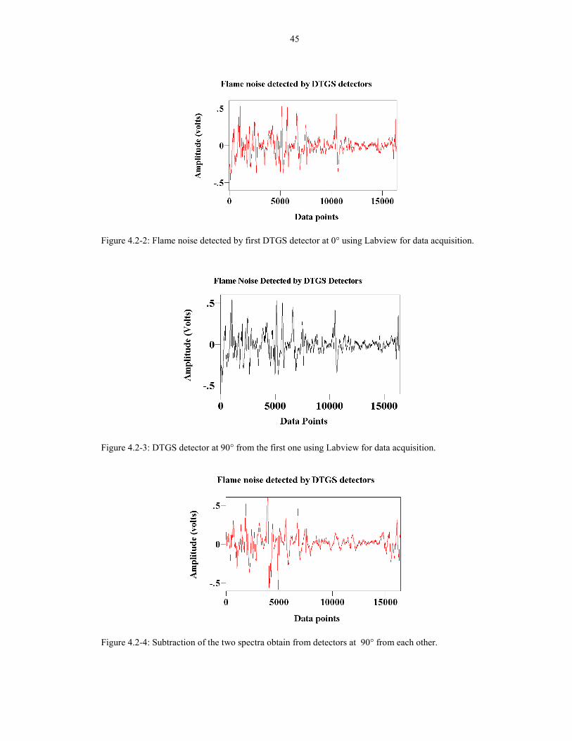
Figure 4.2-2 Flame noise detected by first DTGS detector at 0! 45using Labview for data acquisition.

Figure 4.2-3 DTGS degree at 90! from the first one using 45Labview for data acquisition.

Figure 4.2-4 Subtraction of the two spectra obtain at 90! 45from each other.

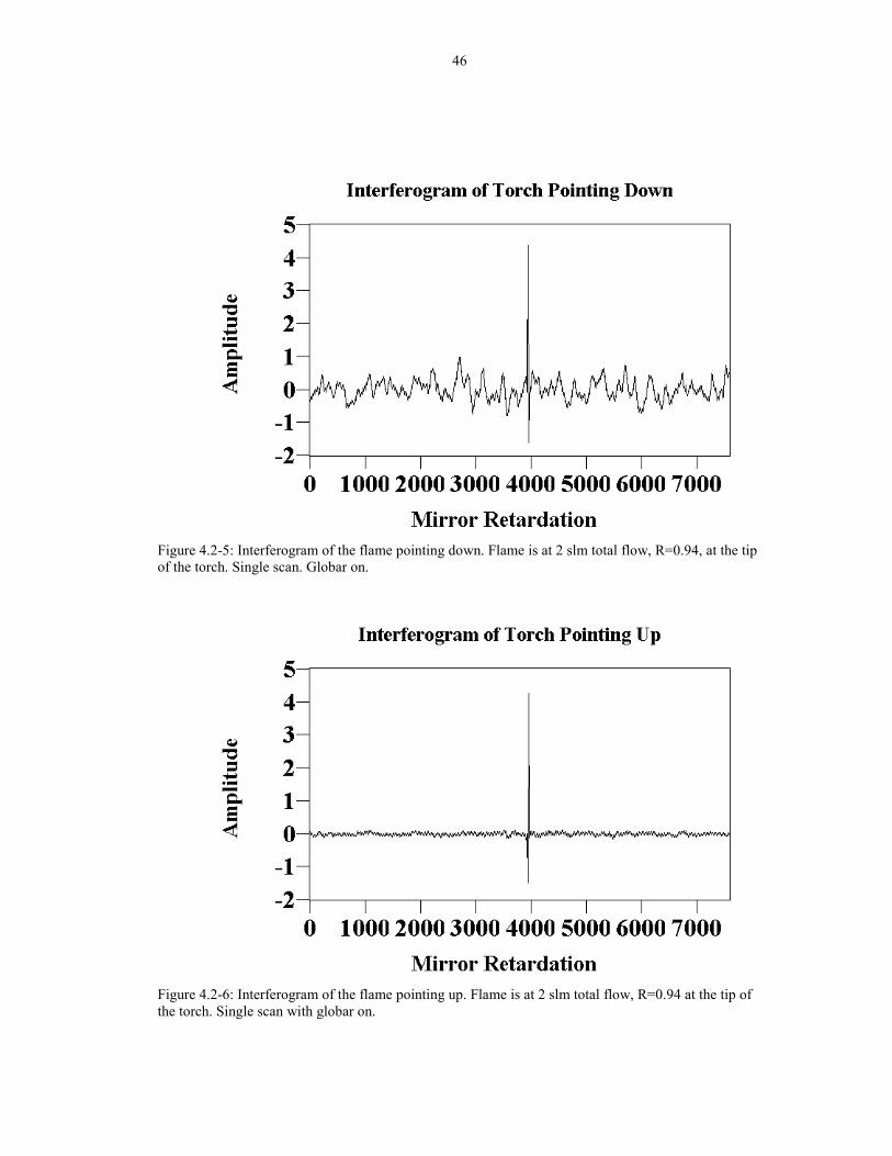
Figure 4.2-5 Interferogram of the flame pointing down. 46Flame is at 2 slm total flow, R=0.94 at the tip of the torch.Single scan. Globar on.

Figure 4.2-6 Interferogram of the flame pointing up. Flame 46is at 2 slm total flow, R=0.94 at the tip of the torch. Singlescan with globar on.

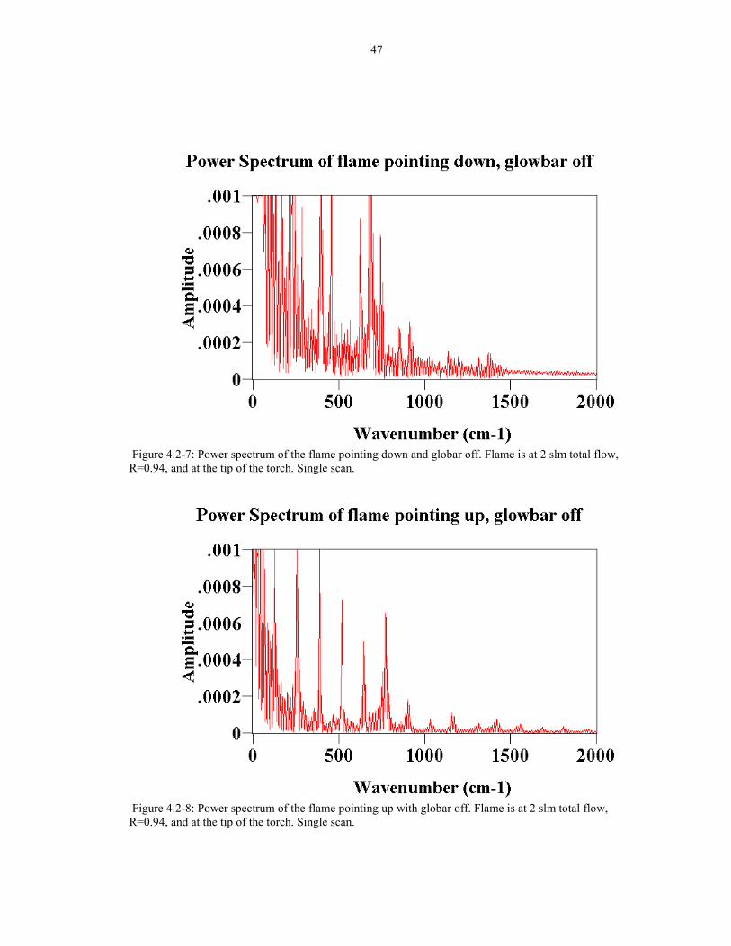
Figure 4.2-7 Power spectrum of the flame pointing down and 47globar off. Flame is at 2 slm total flow, R=0.94 at the tip ofthe torch. Single scan.

Figure 4.2-8 Power spectrum of the flame pointing up with 47globar off. Flame is at 2 slm total flow, R=0.94 at the tip ofthe torch. Single scan.

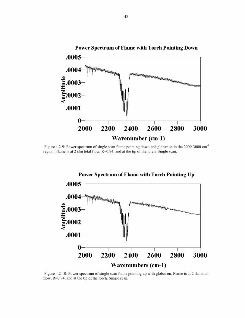
Figure 4.2-9 Power spectrum of single scan flame pointing down 48and globar on in the 2000-3000 cm-1 region. Flame is at 2 slmtotal flow, R=0.94 at the tip of the torch. Single scan.

Figure 4.2-10 Power spectrum of single scan flame pointing up 48with globar on. Flame is at 2 slm total flow, R=0.94 at the tip ofthe torch. Single scan.

x

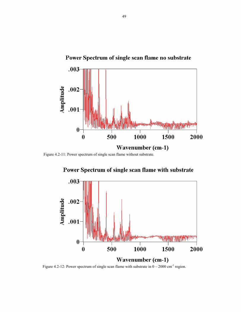
Figure 4.2-11 Power spectrum of single scan flame without substrate. 49

Figure 4.2-12 Power spectrum of single scan flame with substrate 49in 0 �2000 cm-1 region.

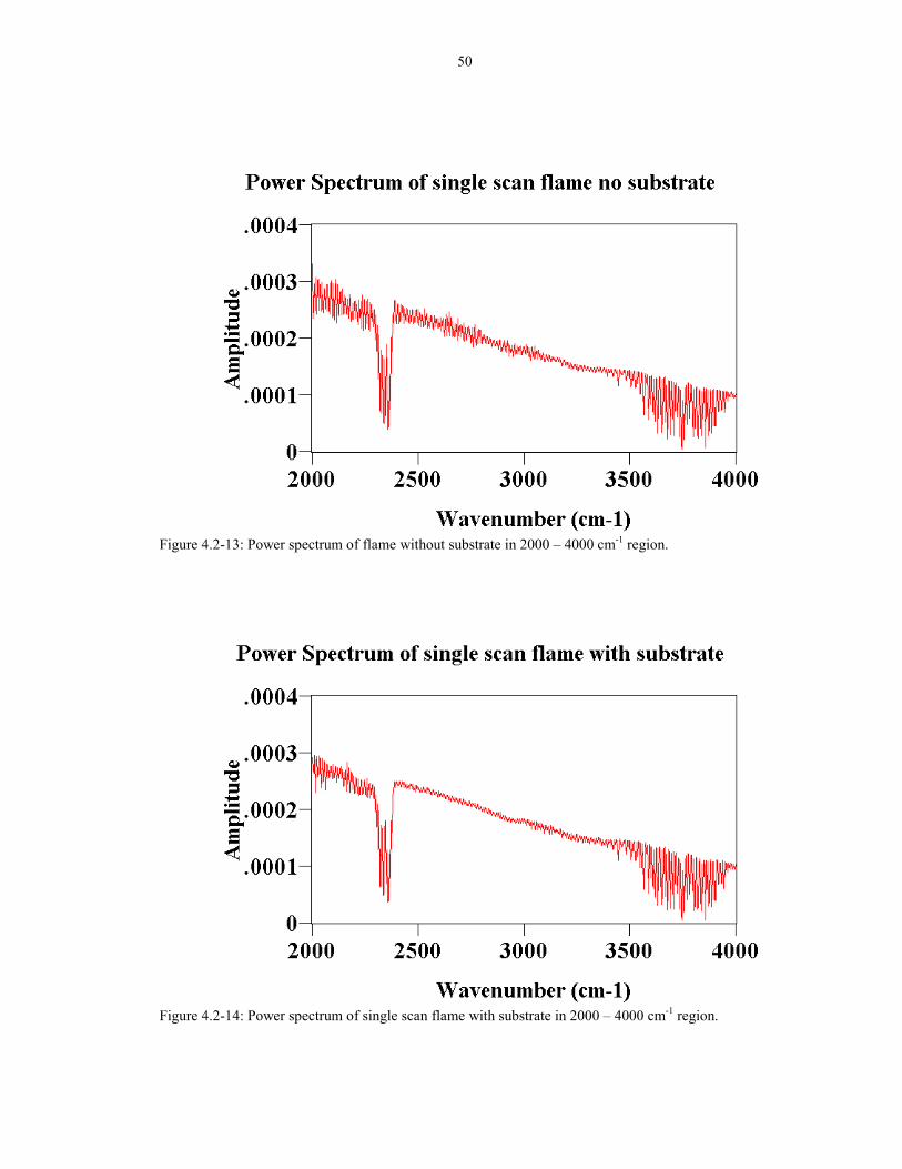
Figure 4.2-13 Power spectrum of flame with out substrate in 502000-4000 cm-1 region.

Figure 4.2-14 Power spectrum of single scan flame with substrate 50in 2000-4000 cm-1 region.

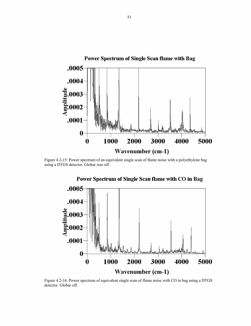
Figure 4.2-15 Power spectrum of a equivalent single scan of 51flame noise with a polyethylene bag using a DTGS detector.Globar was off.

Figure 4.2-16 Power spectrum of equivalent single scan of flame 51noise with CO in bag using DTGS detector. Globar off.

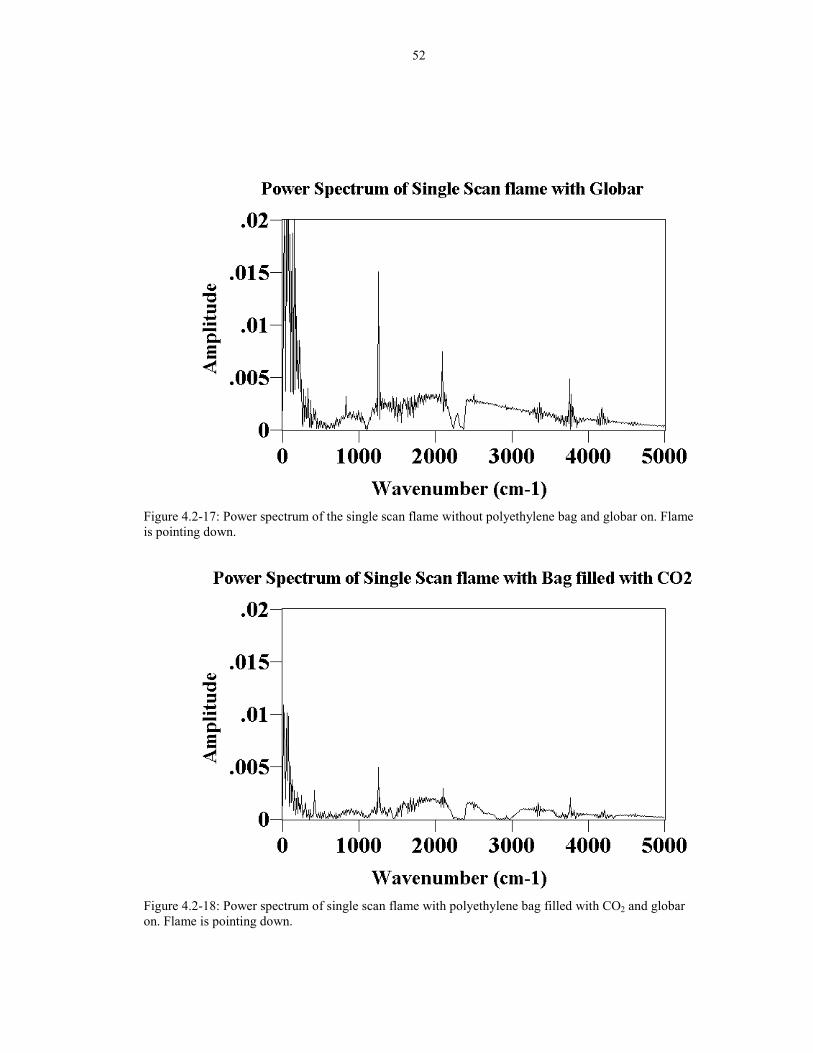
Figure 4.2-17 Power spectrum of the single scan flame without 52polyethylene bag and globar on. Flame is pointing down.

Figure 4.2-18 Power spectrum of single scan flame with 52polyethylene bag filled with CO2 and globar on. Flame ispointing down.

Figure 4.2-19 Transmission spectrum of the infared filter. 53This was taken at cm-1 using a DTGS detector. Single scan.

Figure 4.2-20 Power spectrum of a flame pointing down 53without filter. Globar is on, single scan.

Figure 4.2-21 Power spectrum of a single scan flame pointing 54down with filter. Globar is on, single scan.

Figure 5.1-1 Calculated Radiance from the transmission data: 71(1-transmission)*blackbody(1900K). Flame conditions: Totalflow = 2 slm R=0.90 at 0 mm position.

Figure 5.1-2 Experimental radiance. Flame conditions: Total 71flow = 2 slm R=0.90 at 0 mm position.

Figure 5.2-1 Experimental spectra of the CO2 hot emission bands. 72Flame conditions: Total flow = 2 slm R=0.90 at 0 mm position.

xi

Figure 5.2-2 Overlap spectra of experimental and HITRAN92 72(0.013 atm cm CO2 in 1 atm 2500K; Voigt lineshape) calculated.Flame conditions: Total flow = 2 slm R=0.90 at 0 mm position.

Figure 5.3-1 Calculated Spectrum from HITRAN96 0.11 atm cm 73in 1 atm at 2700K; Voigt lineshape.

Figure 5.3-2 Combined spectra of calculated CO (0.11 atm cm in 731 atm 2700K, HITRAN96 Voigt lineshape) and CO2 (0.013 atmcm 2500K, HITRAN92 Voigt lineshape).

Figure 5.3-3 Comparing calculated spectrum to experimental 74spectrum. Calculated parameters: CO2: 0.013 atm cm in 1 atm2500K Voigt lineshape. CO: 0.11 atm cm in 1 atm 2700K Voigtlineshape. Experimental conditions: Total flow = 2 slm R=0.90at 0 mm position.

Figure 5.3-4 Experimental Spectrum of flame: Total flow = 2 slm 74R=1.10 at 0 mm position.

Figure 5.3-5 Difference of R = 0.90 minus R=1.10. Experimental 75conditions: Ft=2 slm at the 0 mm position.

Figure 5.4-1 Experimental and calculated spectra in the water 75band region. Calculated paramters: HITEMP 0.03 atm cm in1 atm Voigt lineshape at 3000K and 1900K Flame conditions:Ft=2 slm R=0.90 at 0 mm position.

Figure5.4-2 Experimental (0 mm position, R=0.90, Ft=2 slm ) 76plotted with the calculated water bands (0.03 atm cm 3000K)Calculated spectrum is offset for clarity.

Figure 5.4-3 Comparison of room temperature water with 3000K 77water transmission. Calculated parameters: 1 atms total, Voigtlineshape. HITEMP.

Figure 5.4-4 Transmission spectrum of 0 mm position aith 77R =0.90 showing hot water bands.

xii

Figure 5.5-1 Experimental (0 mm position R=0.90 Open flame, 78Ft=2slm) plotted with the calculated spectra including the OH.bands H2O: 0.03 atm cm in 1 atm at 3000K HITEMP; Voigt.lineshape OH: 0.006 atm cm in 1 atm HITRAN 96; Voigtlineshape. Calculated spectrum is offset for clarity.

Figure 5.5-2 Calculated spectrum minus experimental spectrum 78for the water band region. Taken from flame position 0 mm withR = 0.90 Ft=2 slm. Calculated parameters: H2O: 0.03 atm cm in1 atm at 3000K HITEMP Voigt lineshape. OH: 0.006 atm cm in1 atm HITRAN 96; Voigt lineshape; * denotes 3587 cm-1 band.

Figure 5.6-1: Comparing calculated to experimental acetylene 79peak at 730 cm-1. Experimental conditions: 0.048 atm in 1 atm,15 cm pathlength, and 300K. Calculated parameters: 0.048 atm,in 1 atm 15 cm, 300K, and Voigt lineshape.

Figure 5.6-2: Comparing calculated to experimental acetylene 79peak at 3280 cm-1. Experimental conditions: 0.048 atm in 1 atm,15 cm pathlength, and 300K. Calculated parameters: 0.048 atmin 1 atm, 15 cm, 300K, and Voigt lineshape.

Figure 5.6-3 Experimental and calculated absorbance acetylene 80spectrum Flame conditions: 0 mm position, Total Flow = 2 slmand R=0.90 Calculated parameters: 0.007 atm cm in 1 atm 400KHITRAN 96; Voigt lineshape. Spectra shifted for clarity.

Figure 5.6-4 Experimental minus Calculated absorbance spectra 80in the acetylene region for 0 mm position; from Figure 5.6-1.

Figure 5.6-5 Comparing the acetylene bands at 300K with 81experimental. Calculated spectrum shifted for clarity.Calculation parameters: 0.005 atm in 1 atm, 1 cm pathlength,300K, Voigt lineshape, HITRAN 92.

Figure 5.6-6 Comparing Experimental Absorbance with 81calculated acetylene at 500K (0.005 atm cm in 1 atm Voigt lineshapeHITRAN96). Calculated spectrum shifted for clarity.

Figure 5.6-7 Comparing acetylene (400K) with experimental 82spectrum (0 mm position R=0.90) at the 730cm-1 acetylene peaks.

xiii

Figure 5.6-8 Plot of concentrations as a function of distance for 82R=0.90 Ft=2 slm.

Figure 5.6-9: Plot of concentration as a function of distance at 83R=0.94 Ft=2 slm.

Figure 5.6-10: Plot of concentration versus distance for R=0.98. 83

Figure 5.6-11: Plot of concentration versus distance for R=1.04. 84

Figure 5.6-12: Plot of concentration versus distance for R=1.10. 84

Figure 5.6-13: Plot of oxygen entrainment for different R ratios. 85

Figure 5.6-14: Plot of calculated hydrogen for various R values 85and position.

Figure 6.1-1: Single beam spectra of two different detectors 99(nonlinear and linearized). Taken at 50 scans at 1cm-1 resolution.Spectra are of the background.

Figure 6.1-2: Absorbance spectra of the flame at total flow of 2 slm 99with R=0.90. Two different detectors are shown.

Figure 6.1-3: Absorbance spectra of the standard and linearized 100detector in the CO2 region. It was taken through the flame withtotal flow rate of 2 slm and R=0.90

Figure 6.1-4: Two background spectrum (one with purge in arm 100and one without) shown here are taken with 2 scans at 1 cm-1 resolution.

Figure 6.2-1: Emission spectrum of enclosed flame at Ft = 2 slm, 1010 mm position, and R=0.90: Shown with a greybody calculated by(1-transmission spectra) * Blackbody at 450K.

Figure 6.2-2: Transmission spectrum of the enclosed flame at 101Ft=2 slm, 0mm position, and R=0.90.

Figure 6.2-3: Emission spectrum of the flame at Ft=2 slm, 1026 mm position, and R=0.90.

Figure 6.2-4: Transmission spectrum of the enclosed flame at 1026 mm position and R=0.90.

xiv

Figure 6.3-1: Emission and transmission enclosed flame spectrum 103at Ft= 2 slm, 0 mm position, and R=0.90.

Figure 6.3-2: E/T analysis of the enclosed flame for CO at Ft=2 slm, 1030 mm position, and R=0.90. Shown above is the matching of thehot CO bands at 1200K.

Figure 6.3-3: The enclosed flame at Ft=2 slm, 0 mm position, 104and R=0.90 showing that the hot CO bands indicates a temperaturehigher than 1200K. Simulated spectrum (top) does not match theexperimental shape (bottom).

Figure 6.3-4: The emission spectrum of the flame at Ft=2 slm, 1040 mm position, and R=0.90 compared to calculated spectrumof 0.05 atm cm in 1 atm CO at 2500K using HITRAN96 Voigt.

Figure 6.4-1: Enclosed flame at Ft=2 slm, 0 mm position, and R=0.90 105showing the presence of hot CO2 bands. CO2 calculation parameters:0.01 atm cm in 1 atm, 600K, HITRAN92, Lorentzian line shape.

Figure 6.4-2: Enclosed flame at Ft=2 slm, 0 mm position, and R=0.90 105showing the approximate concentration of CO2.Calculated CO2: 0.003 atm cm in 1 atm, 2000K, HITRAN92 Voigt lineshape.

Figure 6.6-1: Experimental (Ft=2 slm, 0 mm position, R=0.90) and 106calculated OH (0.0032 atm cm in 1 atm at 3000K HITRAN96 Voigt)spectra. No OH is present in the flame at 0 mm position R=0.90.

Figure 6.6-2: Enclosed flame at Ft=2 slm, 18 mm position ,and R=0.90 106shows no observable OH peaks. Calculation parameters for OH:0.0032 atm cm in 1 atm 3000K , HITRAN96 Voigt

Figure 6.8-1: Methane at two different temperatures showing 107difference in side peaks. Calculation parameters: 0.01 atm cmin 1 atm, HITRAN92 Voigt at 500K and 800K.

Figure 6.8-2: Enclosed flame at Ft= 2 slm, 0 mm position and 107R=0.90 in the methane region. Calculated parameters:0.002 atm in 1atm 400K HITRAN92 Voigt

Figure 6.9-1: Free enclosed flame: concentration versus position at R=0.90 108

Figure 6.9-2: Free enclosed flame: concentration versus position at R=0.94 108

xv

Figure 6.9-3: Free enclosed flame: concentration versus position at R=0.98 109

Figure 6.9-4: Free enclosed flame: concentration versus position at R=1.04 109

Figure 6.9-5: Free enclosed flame: concentration versus position at R=1.10 110

Figure 6.9-6: Free enclosed flame: H2 calculated versus position 110

Figure 6.9-7: Free enclosed flame: O2 entrainment calculation versus position 111

1

1.0 INTRODUCTION

1.1 Diamond Films and Its Applications

Diamond has many useful properties. It has a high hardness, high thermal

conductivity, high electrical resistivity, high wear resistance, low coefficient of

friction, is chemically inert, and is optically transparent from ultraviolet to far

infrared. [1-4] With all these properties, diamond is a very attractive material for

many applications. These applications include scratchproof coatings, cutting tool

coating, and heat sinks in the electronic industry.

1.2 CVD Methods

There are several methods of depositing diamond films by chemical vapor

deposition including the use of a hot filament, microwave plasma, or oxyacetylene

torch. In a hot filament reactor, methane and hydrogen are introduced near a hot

filament heated to 2000-2500K. The purpose of the hot filament is to dissociate the

gas mixture into radicals. This method is usually carried out at low pressures (about

20 Torr) and results in a low growth rate (approximately 0.1 to 1 µm/hr) while

attaining high quality diamond films. [1, 5] Microwave plasma is also used to deposit

diamond films on various substrates. [1, 6, 7] Typically, a polished silicon substrate is

placed in a cavity where the pressure is lowered to about 1 mTorr. Then a hydrogen

plasma is ignited with the microwave power. After the plasma is ignited, the pressure

is incrementally increased (to about 20 Torr) and methane and perhaps oxygen

containing species are then added to the plasma for diamond deposition. [8, 9]

2

However, there has been interest to grow these diamond films at higher growth

rates while minimizing the cost of the equipment. One method for diamond film

synthesis that meets these criteria is the use of an oxyacetylene torch. Previous

research has reported that at atmospheric pressure, the linear growth rate is

approximately 100-200 µm per hour. [10, 11] In the oxyacetylene torch method,

mass flow controllers control the flow of oxygen and acetylene to the torch. The

premixed gases then form the combustion flame at the nozzle. Figure 1.0-1 shows a

schematic of the flame. There are three primary regions in an open flame: inner cone,

feather, and the outer flame. In the inner cone, the gases are hot and not yet reacting

significantly. In the region between the inner cone and feather, the gases react

according to the overall reaction:

C2H2 + O2 2 CO + H2 (1.2-1)

In the outer flame, secondary combustion produces carbon dioxide and water:

2 CO + H2 + 3/2 O2 2 CO2 + H2O (1.2-2)

The secondary combustion accounts for about 2/3 of the total heat released in the

combustion of acetylene. A water-cooled substrate, usually molybdenum, is inserted

inside the flame about one mm from the inner cone. [12] The temperature of the

substrate is measured by a two-color pyrometer or a thermocouple. It has been

determined that the oxygen to acetylene flow ratio (R) is one of the primary factors

that determine the quality of the diamond films. The typical flow rate used is about 2-

3 L/min total flow rate with an R ratio of about 0.93-0.99. [12]

3

Diamond films have been grown systematically in open and enclosed flames. [12-

16] In the case of enclosed flames, the secondary combustion in the outer flame

disappears. Despite this large change in the chemistry (Equations 1.2-1 and 1.2-2), the

only major effect of enclosing the flame is lowering the growth rate. [16]

1.3 The Purpose of This Work

The purpose of this work is to better understand the chemistry of diamond CVD

using the oxyacetylene torch system. The analysis technique is in situ Fourier

transform infrared spectroscopy. This extends the work of Morrison et al. [17] in

which they perform in situ FTIR measurements of the oxyacetylene flame using the

emission and transmission method. The present work compares the tomographic

reconstruction of FTIR measurements of a deposition flame. [18] A free flame

without a substrate is analyzed in an open and enclosed atmosphere at various axial

distances from the torch nozzle ranging from 0 mm to 18 mm. In addition, the R ratio

is varied over a range of R = 0.90 to 1.10.

The methodology combines the emission and transmission FTIR measurements to

determine the species concentration and gas temperature as a function of R and

position. Species under study include CO, CO2, H2O, OH, C2H2, and CH4. The

HITRAN database with HITRAN-PC version 2.51 (developed by University of South

Florida and distributed by Ontar Corporation) aids in characterizing these species.

4

Figure 1.0-1 Regions of the acetylene flame.

5

2.0 PRIOR RESEARCH

2.1 Open Flames

Many authors have determined the range of deposition parameters for diamond

growth, and Morrison and Glass [1] have reviewed much of the work prior to 1993. A

brief summary of those works, as well as newer research, is presented here.

Hirose and Amanuma [2] found that diamond growth can occur between R = 0.7

to 1.0. Amorphous carbon was formed when the R ratio was less than 0.7, and the

etching of diamond occurred when R is greater than 1.0. The range of temperature for

diamond deposition was found to be 370 � 1200 °C. The best diamond films were

grown when the R ratio was between 0.85 to 0.98. Wang et al. [3] found similar

conditions for diamond growth using an R ratio between 0.89 and 0.99 with a

temperature range of 650-1320°C. On the contrary, Hanssen et al. [4] reported

diamond growth under both fuel rich and oxygen rich conditions: R = 0.9 to 1.08.

Schermer et al. [5] found that a supersaturation of 6 % (percentage of extra C2H2

flow compared to the neutral flame conditions) at a temperature of 1200 °C to be

optimum. The supersaturation is defined as:

an

ana

FFFaionSupersatur −= (2.1-1)

where Fa = flow of acetylene and Fan = flow of acetylene of neutral flame.

Solving for R (the ratio of oxygen flow to acetylene flow) the supersaturation is

related to R via:

6

ationSupersaturRRn =−1 (2.1-2)

where Rn = R value at neutral flame condition. In the torch system used for this

experiment, the neutral flame occurs when R = 1.03. Therefore, a supersaturation of

6% yields an R value of 0.97.

In addition, many authors have researched oxyacetylene CVD since 1993. Bang et

al. [6] studied the effect of nozzle size and substrate temperature on the quality of

diamond. At a fixed R = O2/C2H2 = 0.98, he found that the lower limit on

temperature for any diamond deposition was 680 °C. Two nozzle sizes were studied

in these experiments. They found that the 0.939 mm diameter nozzle deposited better

diamond films than the 1.067 mm diameter nozzle under identical growing

conditions. Zeatoun and Morrison [7] found that high R ratio (0.97-0.99) along with

either high (1000°C) or low (800°C) surface temperature, depending on the total flow

rate, to be optimum. Marinkovic et al. [8] were able to deposit large diamond crystals,

about 200 µm in size, on a molybdenum substrate with the R ratio = 0.93 to 0.98,

surface temperature of 700-765°C, and a total flow rate of 3.8 to 5.2 L/min. The total

deposition time was one to four hours. Zhu et al. [9] were able to grow high quality

diamond at R = 0.96 and surface temperature of 750 °C. Using Raman spectroscopy

to analyze the film, their diamond has a FWHM of 4.5 cm-1, which is within the top

quality range of synthetic CVD diamonds. Zhang et al. [10] calculated phase

diagrams using thermodynamics for diamond growth in an oxyacetylene flames. They

compared their results to many different authors� experimental results and found that

7

the calculated phase diagrams correlate very nicely with the experimental results. In

the diagram, it is predicted that diamond growth occurs when the R ratio is between

0.8 and 1.1 with the surface temperature between 1000-1250K. This is consistent with

many experimental results. [2, 4, 11, 12]

2.2 Enclosed Flames

There have been many studies on the effect of the atmosphere on the oxyacetylene

flame under diamond growing conditions. Murakawa et al. [13] eliminated the outer

flame by covering the flame and thus were able to increase the deposition area to 40

mm x 40 mm at a lower growth rate. Murakawa and Takeuchi [14] deposited

diamond films on cemented carbide and compared the performance of the diamond

films grown using an enclosed flame to that of an open flame. In addition, they found

that the heat load decreased by a factor of 1/3 because the overall reaction in the

enclosed flame is

C2H2 + O2 CO + H2 (1.2-1)

instead of

C2H2 + (5/2) O2 CO2 + H2O (1.2-2)

The heat of reaction in (1.2-1) accounts for 1/3 of the heat of reaction in (1.2-2). In

addition to the lower heat load, they found that the deposition area increased by 50%

and the size of individual grains decreased.

Doverspike et al. [15] shrouded the flame with a flow of argon to eliminate the

outer flame. These diamond films had smooth (100) faces with more amorphous

8

carbon. Morrison et al [16] deposited diamond films with the enclosed flame on

silicon. They found that the growth rate was approximately ten times slower than that

of the open flame. This may have been due to an increased in deposition area,

decreasing the linear growth rate. The deposition area, however, was about 2.5 times

higher than in the open flame. They also found that the Raman spectra of the enclosed

flame to be similar to that of cycling the R ratio. [17, 18] They found the best

diamond growth in high temperature (900 °C) and high R ratio (0.96-0.97).

2.3 Diagnostics and Flames

2.3.1 Optical Emission Spectroscopy

Matsui et al. [19] found intense emission of the excited states CH* and C2*

localized in the feather boundary. The OH* emission is localized in the intermediate

zone, right outside of the feather. In other work, Yalamanchi et al. [20] found C*, C2*,

CH*, molecular H2*, atomic H*, and atomic O* in the feather region. They also

observed C2* and CH* in the intermediate zone, just outside of the feather. However,

lower values of CH* were found in the intermediate zone compared to the primary

combustion zone. In addition, when the torch was operated under fuel rich conditions,

excess H*, OH*, and O* were also observed outside of the feather. The flame

temperature reported here was 3237K.

2.3.2 Laser induced fluorescence

Matsui et al. [21] used mass spectrometric techniques to find that the main gaseous

species in the feather region were CO and H2. They then used LIF to analyze for C2

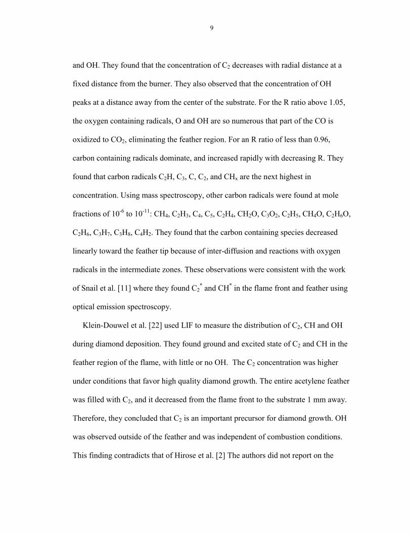
9

and OH. They found that the concentration of C2 decreases with radial distance at a

fixed distance from the burner. They also observed that the concentration of OH

peaks at a distance away from the center of the substrate. For the R ratio above 1.05,

the oxygen containing radicals, O and OH are so numerous that part of the CO is

oxidized to CO2, eliminating the feather region. For an R ratio of less than 0.96,

carbon containing radicals dominate, and increased rapidly with decreasing R. They

found that carbon radicals C2H, C3, C, C2, and CHx are the next highest in

concentration. Using mass spectroscopy, other carbon radicals were found at mole

fractions of 10-6 to 10-11: CH4, C2H3, C4, C5, C2H4, CH2O, C3O2, C2H5, CH4O, C2H6O,

C2H6, C3H7, C3H8, C4H2. They found that the carbon containing species decreased

linearly toward the feather tip because of inter-diffusion and reactions with oxygen

radicals in the intermediate zones. These observations were consistent with the work

of Snail et al. [11] where they found C2* and CH* in the flame front and feather using

optical emission spectroscopy.

Klein-Douwel et al. [22] used LIF to measure the distribution of C2, CH and OH

during diamond deposition. They found ground and excited state of C2 and CH in the

feather region of the flame, with little or no OH. The C2 concentration was higher

under conditions that favor high quality diamond growth. The entire acetylene feather

was filled with C2, and it decreased from the flame front to the substrate 1 mm away.

Therefore, they concluded that C2 is an important precursor for diamond growth. OH

was observed outside of the feather and was independent of combustion conditions.

This finding contradicts that of Hirose et al. [2] The authors did not report on the

10

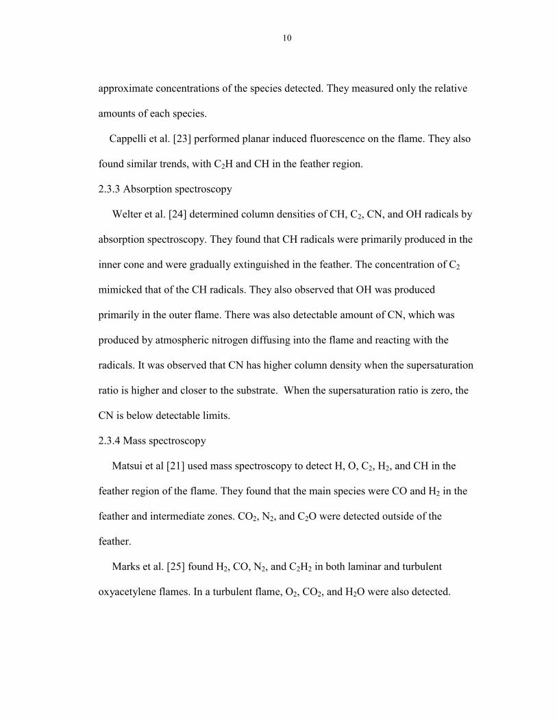
approximate concentrations of the species detected. They measured only the relative

amounts of each species.

Cappelli et al. [23] performed planar induced fluorescence on the flame. They also

found similar trends, with C2H and CH in the feather region.

2.3.3 Absorption spectroscopy

Welter et al. [24] determined column densities of CH, C2, CN, and OH radicals by

absorption spectroscopy. They found that CH radicals were primarily produced in the

inner cone and were gradually extinguished in the feather. The concentration of C2

mimicked that of the CH radicals. They also observed that OH was produced

primarily in the outer flame. There was also detectable amount of CN, which was

produced by atmospheric nitrogen diffusing into the flame and reacting with the

radicals. It was observed that CN has higher column density when the supersaturation

ratio is higher and closer to the substrate. When the supersaturation ratio is zero, the

CN is below detectable limits.

2.3.4 Mass spectroscopy

Matsui et al [21] used mass spectroscopy to detect H, O, C2, H2, and CH in the

feather region of the flame. They found that the main species were CO and H2 in the

feather and intermediate zones. CO2, N2, and C2O were detected outside of the

feather.

Marks et al. [25] found H2, CO, N2, and C2H2 in both laminar and turbulent

oxyacetylene flames. In a turbulent flame, O2, CO2, and H2O were also detected.

11

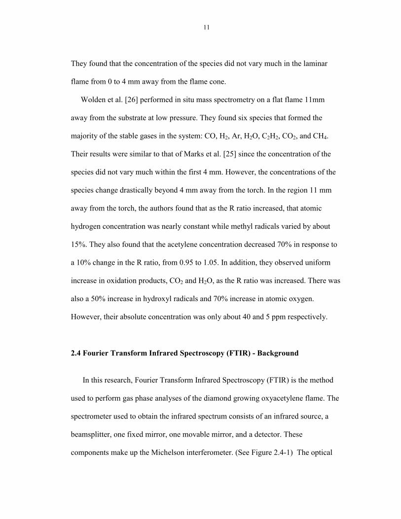
They found that the concentration of the species did not vary much in the laminar

flame from 0 to 4 mm away from the flame cone.

Wolden et al. [26] performed in situ mass spectrometry on a flat flame 11mm

away from the substrate at low pressure. They found six species that formed the

majority of the stable gases in the system: CO, H2, Ar, H2O, C2H2, CO2, and CH4.

Their results were similar to that of Marks et al. [25] since the concentration of the

species did not vary much within the first 4 mm. However, the concentrations of the

species change drastically beyond 4 mm away from the torch. In the region 11 mm

away from the torch, the authors found that as the R ratio increased, that atomic

hydrogen concentration was nearly constant while methyl radicals varied by about

15%. They also found that the acetylene concentration decreased 70% in response to

a 10% change in the R ratio, from 0.95 to 1.05. In addition, they observed uniform

increase in oxidation products, CO2 and H2O, as the R ratio was increased. There was

also a 50% increase in hydroxyl radicals and 70% increase in atomic oxygen.

However, their absolute concentration was only about 40 and 5 ppm respectively.

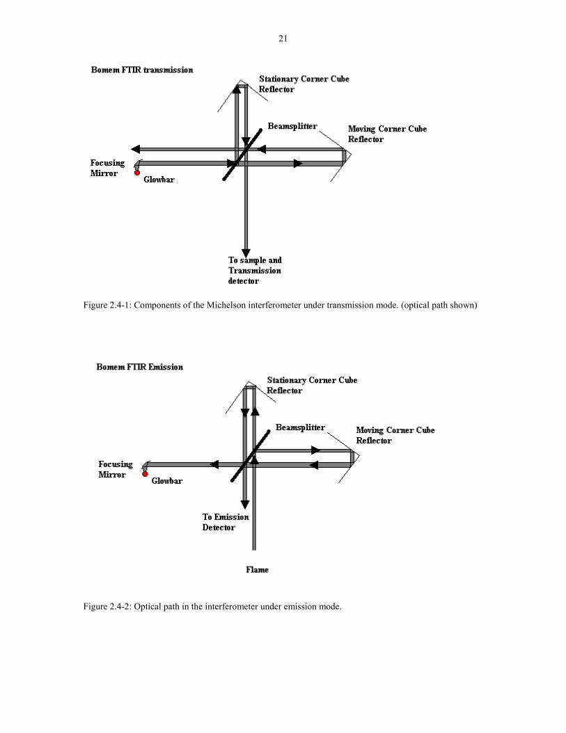
2.4 Fourier Transform Infrared Spectroscopy (FTIR) - Background

In this research, Fourier Transform Infrared Spectroscopy (FTIR) is the method

used to perform gas phase analyses of the diamond growing oxyacetylene flame. The

spectrometer used to obtain the infrared spectrum consists of an infrared source, a

beamsplitter, one fixed mirror, one movable mirror, and a detector. These

components make up the Michelson interferometer. (See Figure 2.4-1) The optical

12

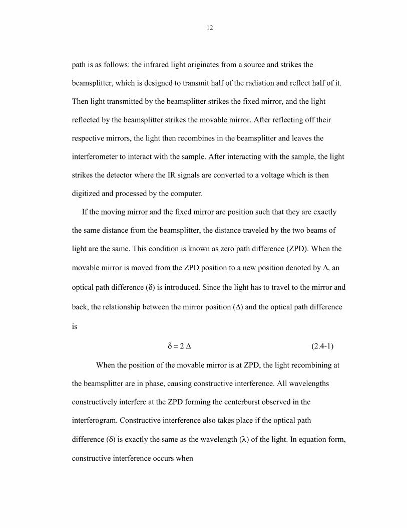
path is as follows: the infrared light originates from a source and strikes the

beamsplitter, which is designed to transmit half of the radiation and reflect half of it.

Then light transmitted by the beamsplitter strikes the fixed mirror, and the light

reflected by the beamsplitter strikes the movable mirror. After reflecting off their

respective mirrors, the light then recombines in the beamsplitter and leaves the

interferometer to interact with the sample. After interacting with the sample, the light

strikes the detector where the IR signals are converted to a voltage which is then

digitized and processed by the computer.

If the moving mirror and the fixed mirror are position such that they are exactly

the same distance from the beamsplitter, the distance traveled by the two beams of

light are the same. This condition is known as zero path difference (ZPD). When the

movable mirror is moved from the ZPD position to a new position denoted by ∆, an

optical path difference (δ) is introduced. Since the light has to travel to the mirror and

back, the relationship between the mirror position (∆) and the optical path difference

is

δ = 2 ∆ (2.4-1)

When the position of the movable mirror is at ZPD, the light recombining at

the beamsplitter are in phase, causing constructive interference. All wavelengths

constructively interfere at the ZPD forming the centerburst observed in the

interferogram. Constructive interference also takes place if the optical path

difference (δ) is exactly the same as the wavelength (λ) of the light. In equation form,

constructive interference occurs when

13

δ = n λ (2.4-2)

where n is any integer. Destructive interference occurs when the optical path

difference is exactly half of the wavelength:

δ = (n + ½) λ (2.4-3)

When the optical path difference is different that any of the above, a combination of

constructive and destructive interference occurs. A plot of the light intensity versus δ

is called an interferogram.

Since the mirror is moving with a constant velocity, the light going through the

interferometer is time modulated, and the modulation frequency (Fv) for a given

wavenumber is given by

Fv = 2 V ν (2.4-4)

where V = moving mirror velocity, and ν = wavenumber of the light in the

interferometer.

Since each wavenumber causes a constructive and destructive interference at

different optical path difference, light at different wavenumbers are then modulated at

different frequencies. This is how the spectrometer distinguishes signals coming from

different wavenumbers. Each different wavenumber of light gives rise to a sinusoidal

wave of unique frequency measured by the detector. Since the infrared source is

emitting a broadband of infrared light, information on all wavenumbers can be

obtained in a single scan. Since the interferogram is the sum of sinusoidal waves, it

can then be Fourier transformed to obtain the single beam spectrum.

14

By performing multiple scans, the signal to noise ratio of the interferogram can be

significantly improved. The reason is that the signal is added to every scan and the

noise fluctuates randomly. Therefore, by signal averaging, the relative contribution of

the noise to the spectrum are reduced. The signal to noise ratio is proportional to the

square root of the number of scans.

Figure 2.4-2 shows the light path in emission mode. The light from the flame

travels in reverse direction back through the beamsplitter and into the emission

detector located in the emission port of the spectrometer. During the emission mode,

the globar is turned off so that only the IR from the flame are modulated by the

moving mirror. This modulation are detected by the emission detector and converted

to a spectrum the same way as the transmission detector.

2.5 FTIR Spectroscopy and CVD

2.5.1 Emission/transmission measurements

Morrison and Haigis [27] were one of the first to perform emission and

transmission IR measurements on a CVD system, in this case, plasma deposition of

amorphous hydrogenated silicon. The authors used the relationship between the

emission and transmission spectra to determine gas temperature in the plasma:

)],(1[),(

)()( 0g

gbb

TTRRR υτ

υυυ −=−

(2.5-1)

where R(ν) = path corrected radiance spectrum in W/(m2 sr cm-1), ν = wavenumber in

cm-1, Tg = temperature of the gas in K, Ro = background radiance from room

15

temperature surroundings in W/m2 sr cm-1, τ = transmission spectrum, and Rbb =

Planck�s blackbody radiation. This relationship assumes that the transmission detector

is cooled to 77K, making the radiation from the detector negligible. The transmission

spectrum (τ(ν,Tg)) and the path corrected emission spectrum (R(ν)) are the measured

parameters. Rbb(ν,Tg) is Planck�s blackbody function given by:

1

),(2

31

−

=gT

Cgbb

e

CTR ν

νν (2.5-2)

C1=1.191 x 10-8 W/m2 sr (cm-1)4 and C2 = 1.439 K cm and Rbb(ν,Tg) is in W/m2 sr

cm-1. The temperature of the gas for the Planck�s function is the temperature of the

blackbody at which Equation 2.5-1 is satisfied. Given the high temperature of the

flame, the emission at room temperature, Ro, is generally taken to be negligible.

This method was also used by Morrison et al. [28] to study the aerosol synthesis of

TiO2 particles. In this work, the authors used FTIR as an in situ diagnostic tool in the

oxidation of TiCl4 in a premixed methane-oxygen flame. Transmission FTIR yielded

quantitative information on HCl, CO2, and H2O by comparing experimental spectra to

spectra calculated from spectroscopic constants found in the HITRAN database. From

the emission and transmission spectra, the authors were also able to obtain

temperature, composition, and particle characteristics in the electrically modified

flames. This same technique are used in the present analysis of the oxyacetylene

flame.

16

2.5.2 FTIR and oxyacetylene flames

Preliminary measurements by Morrison et al [29] have shown that a combination

of emission and transmission measurements yields species concentration (CO2, H2O,

CO, and OH) and gas temperature. In later measurements, Morrison et al. [30]

reported in situ measurements using the emission and transmission method together

with tomography. They found that the feather of the flame was approximately 3000K

and the temperature decreased slightly in the outer flame. In the radial direction, they

observed that the concentration of CO decreases linearly from the inner cone to the

outer cone, with a high concentration in the feather region. CO2 , H2O, and OH exist

primarily in the outer flame. The authors did not observe any radical species using the

FTIR, and the CO2, H2O, CO, and OH measurements were not quantitative.

2.6 HITRAN Database

The HITRAN database was used to calculate high-resolution optical transmission

spectra of the individual gases. The HITRAN database is a catalogue of spectroscopic

constants of various gases found in the atmosphere including CO2, CO, H2O, OH,

C2H2 , and CH4. A personal computer software package (HITRAN-PC ver. 2.51,

Ontar Corporation) was developed by the University of South Florida to calculate gas

spectra at a given partial pressure, total pressure, and temperature. A description of

the procedures using the HITRAN database can be found in Morrison et al. [31]. The

only change in methodology is the use of the 1996 HITRAN database and HITEMP

17

database in addition to the 1992 database. The 1996 database is an update of the 1992

database plus additional gases. The HITEMP database includes additional hot bands

and rotational levels for CO2, CO, and H2O appropriate to at least 1000K. However, it

was determined that the catalogued CO2 bands in HITEMP are incomplete at

temperatures above 1500K. In addition, the HITRAN-PC software cannot handle the

full set of the spectroscopic constants in the CO database. Therefore, H2O and

sometimes CO (with a some spectral lines omitted) are calculated using the HITEMP

database while the other gases are calculated using either the 1992 or 1996 database.

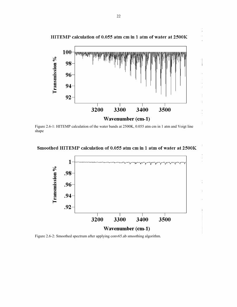
Using HITRAN-PC, a spectrum of a gas can be calculated from spectroscopic

constants in one of the HITRAN databases. The high-resolution spectra (typically

better than 0.01 cm-1) can then be smoothed to a spectra with the same resolution as

those obtained from the FTIR (typically 1cm-1). The method works as follows [31]:

An inverse Fourier Transform is applied to the calculated HITRAN spectrum to

obtain an interferogram. The interferogram is then truncated and apodized to the same

resolution found in the FTIR. These steps mimic the processes that go on inside the

FTIR. The modified spectrum is then Fourier transform back to obtain the 1 cm-1

spectrum. The spectra obtained can then be compared to the experimental spectra to

determine the temperature and quantity of gases present in the flame. Morrison et al.

[31] have verified the accuracy of the procedures outlined above using known

quantities of gas. Morrison et al. have also successfully applied the method to flame

measurements. [28] A sample of a spectra before and after conversion is shown in

Figure 2.6-1 and 2.6-2. A copy of the smoothing program is in Appendix I.

18

In calculating the spectrum for gases in the flame, the wavenumber range was

chosen such that it covers the region of interest and is consistent with the point to

point resolution of the FTIR. In addition, the number of points must be a power of

two. There are three different line shape calculations depending on the conditions and

specie: Doppler, Voigt, and Lorentzian. The choice of line shape depends on the half

width parameter at 296K, the temperature coefficient, the temperature, the total

pressure, the molecular weight, and line position. If the ratio of the Lorentzian line

width to the Doppler line width (Lorentz/Doppler) is less than 0.1, then the Gaussian

line shape is appropriate. [31] If Lorentz/Doppler is between 0.1 and 5, then the Voigt

calculation is appropriate. If the parameter Lorentz/Doppler is greater than 5, then the

Lorentzian calculation is appropriate. Under most condition found in C2H2 / O2

flames, the line shape is typically Voigt.

The Lorentz/Doppler parameter is defined as:

)(7601))296((U

PT

gDL n= (2.6-1)

where L/D = Lorentz/Doppler, g = half width parameter at 296 in (cm-1/atm), T =

temperature of interest in (K), n= temperature coefficient, P= total pressure in (Torr),

and U = Doppler half width half maximum

MTvxU o ))(1058.3( 7−= (2.6-2)

where νo = line position in (cm-1), and M = molecular weight in (g / gmol).

19

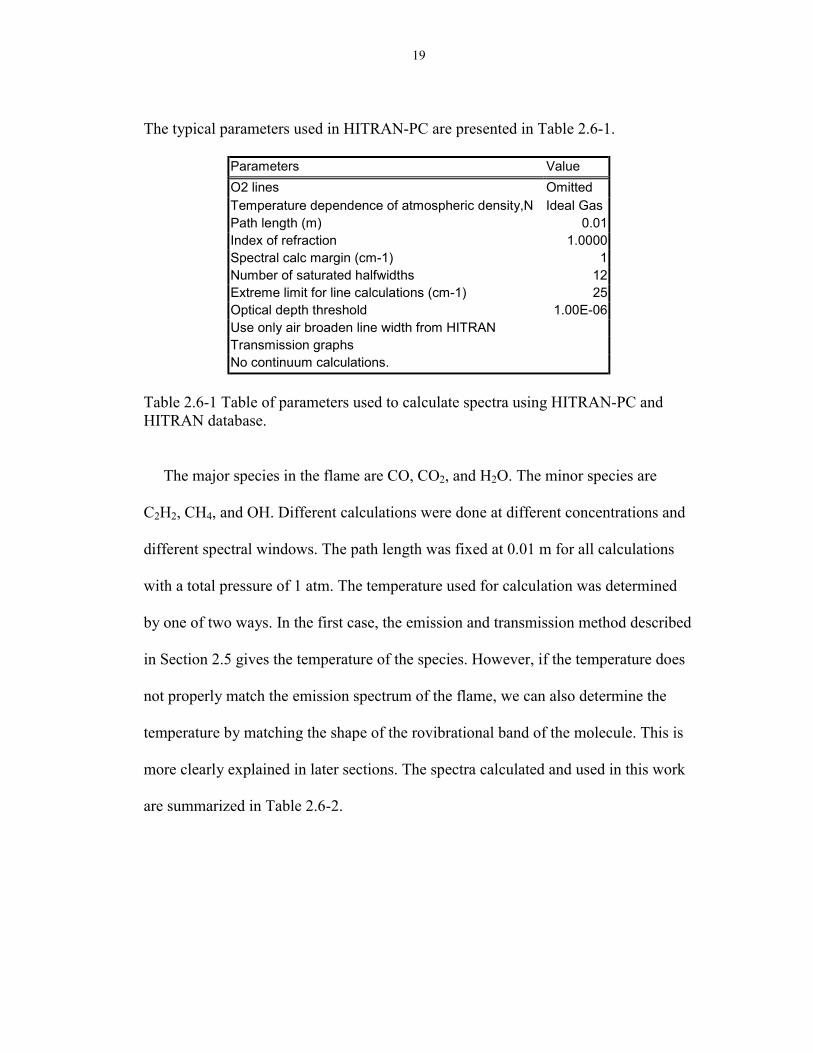
The typical parameters used in HITRAN-PC are presented in Table 2.6-1.

Parameters ValueO2 lines OmittedTemperature dependence of atmospheric density,N Ideal GasPath length (m) 0.01Index of refraction 1.0000Spectral calc margin (cm-1) 1Number of saturated halfwidths 12Extreme limit for line calculations (cm-1) 25Optical depth threshold 1.00E-06Use only air broaden line width from HITRANTransmission graphsNo continuum calculations.

Table 2.6-1 Table of parameters used to calculate spectra using HITRAN-PC andHITRAN database.

The major species in the flame are CO, CO2, and H2O. The minor species are

C2H2, CH4, and OH. Different calculations were done at different concentrations and

different spectral windows. The path length was fixed at 0.01 m for all calculations

with a total pressure of 1 atm. The temperature used for calculation was determined

by one of two ways. In the first case, the emission and transmission method described

in Section 2.5 gives the temperature of the species. However, if the temperature does

not properly match the emission spectrum of the flame, we can also determine the

temperature by matching the shape of the rovibrational band of the molecule. This is

more clearly explained in later sections. The spectra calculated and used in this work

are summarized in Table 2.6-2.

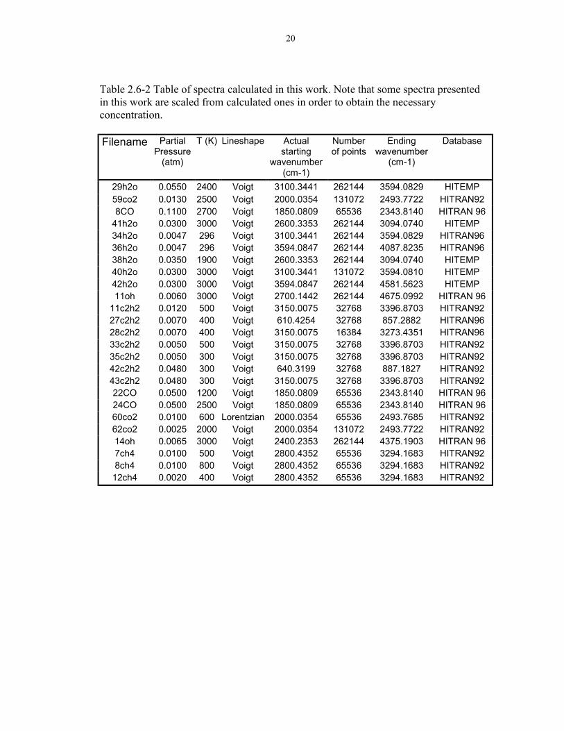
20

Table 2.6-2 Table of spectra calculated in this work. Note that some spectra presentedin this work are scaled from calculated ones in order to obtain the necessaryconcentration.

Filename PartialPressure

(atm)

T (K) Lineshape Actualstarting

wavenumber(cm-1)

Numberof points

Endingwavenumber

(cm-1)

Database

29h2o 0.0550 2400 Voigt 3100.3441 262144 3594.0829 HITEMP59co2 0.0130 2500 Voigt 2000.0354 131072 2493.7722 HITRAN928CO 0.1100 2700 Voigt 1850.0809 65536 2343.8140 HITRAN 96

41h2o 0.0300 3000 Voigt 2600.3353 262144 3094.0740 HITEMP34h2o 0.0047 296 Voigt 3100.3441 262144 3594.0829 HITRAN9636h2o 0.0047 296 Voigt 3594.0847 262144 4087.8235 HITRAN9638h2o 0.0350 1900 Voigt 2600.3353 262144 3094.0740 HITEMP40h2o 0.0300 3000 Voigt 3100.3441 131072 3594.0810 HITEMP42h2o 0.0300 3000 Voigt 3594.0847 262144 4581.5623 HITEMP11oh 0.0060 3000 Voigt 2700.1442 262144 4675.0992 HITRAN 96

11c2h2 0.0120 500 Voigt 3150.0075 32768 3396.8703 HITRAN9227c2h2 0.0070 400 Voigt 610.4254 32768 857.2882 HITRAN9628c2h2 0.0070 400 Voigt 3150.0075 16384 3273.4351 HITRAN9633c2h2 0.0050 500 Voigt 3150.0075 32768 3396.8703 HITRAN9235c2h2 0.0050 300 Voigt 3150.0075 32768 3396.8703 HITRAN9242c2h2 0.0480 300 Voigt 640.3199 32768 887.1827 HITRAN9243c2h2 0.0480 300 Voigt 3150.0075 32768 3396.8703 HITRAN9222CO 0.0500 1200 Voigt 1850.0809 65536 2343.8140 HITRAN 9624CO 0.0500 2500 Voigt 1850.0809 65536 2343.8140 HITRAN 9660co2 0.0100 600 Lorentzian 2000.0354 65536 2493.7685 HITRAN9262co2 0.0025 2000 Voigt 2000.0354 131072 2493.7722 HITRAN9214oh 0.0065 3000 Voigt 2400.2353 262144 4375.1903 HITRAN 967ch4 0.0100 500 Voigt 2800.4352 65536 3294.1683 HITRAN928ch4 0.0100 800 Voigt 2800.4352 65536 3294.1683 HITRAN9212ch4 0.0020 400 Voigt 2800.4352 65536 3294.1683 HITRAN92

21

Figure 2.4-1: Components of the Michelson interferometer under transmission mode. (optical path shown)

Figure 2.4-2: Optical path in the interferometer under emission mode.

22

Figure 2.6-1: HITEMP calculation of the water bands at 2500K, 0.055 atm cm in 1 atm and Voigt lineshape

Figure 2.6-2: Smoothed spectrum after applying conv65.ab smoothing algorithm.

23

3.0 EQUIPMENT DESCRIPTION

3.1 Torch reactor

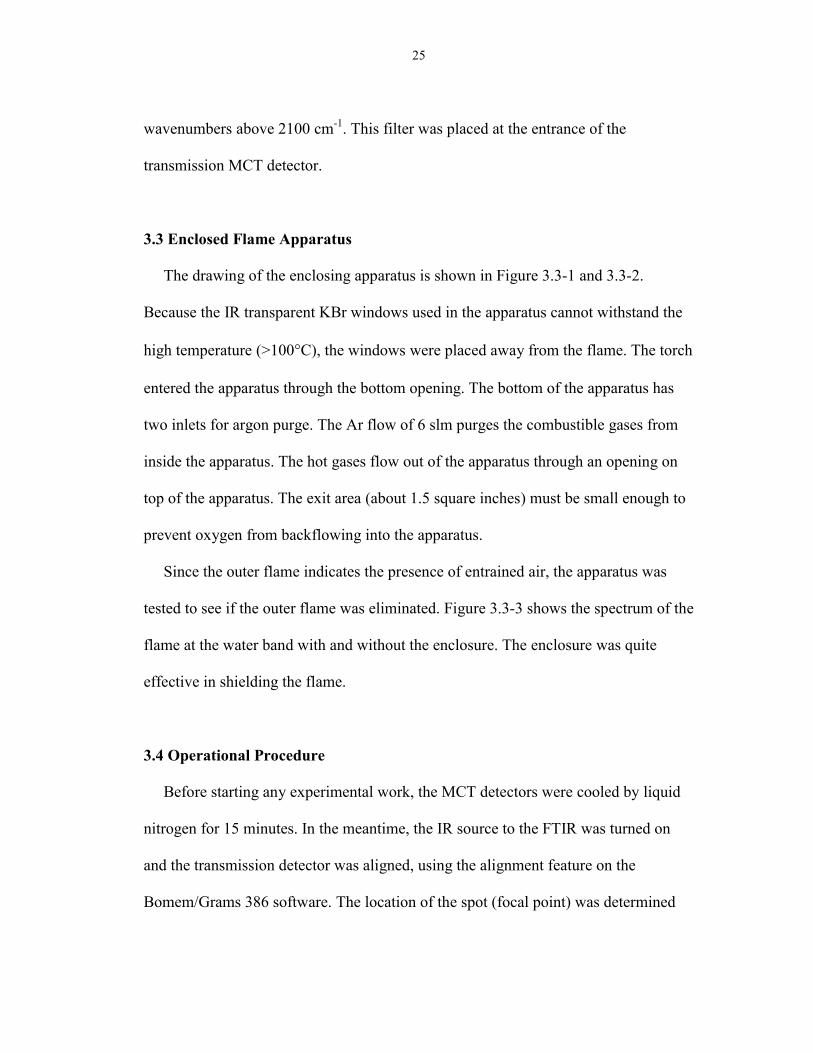
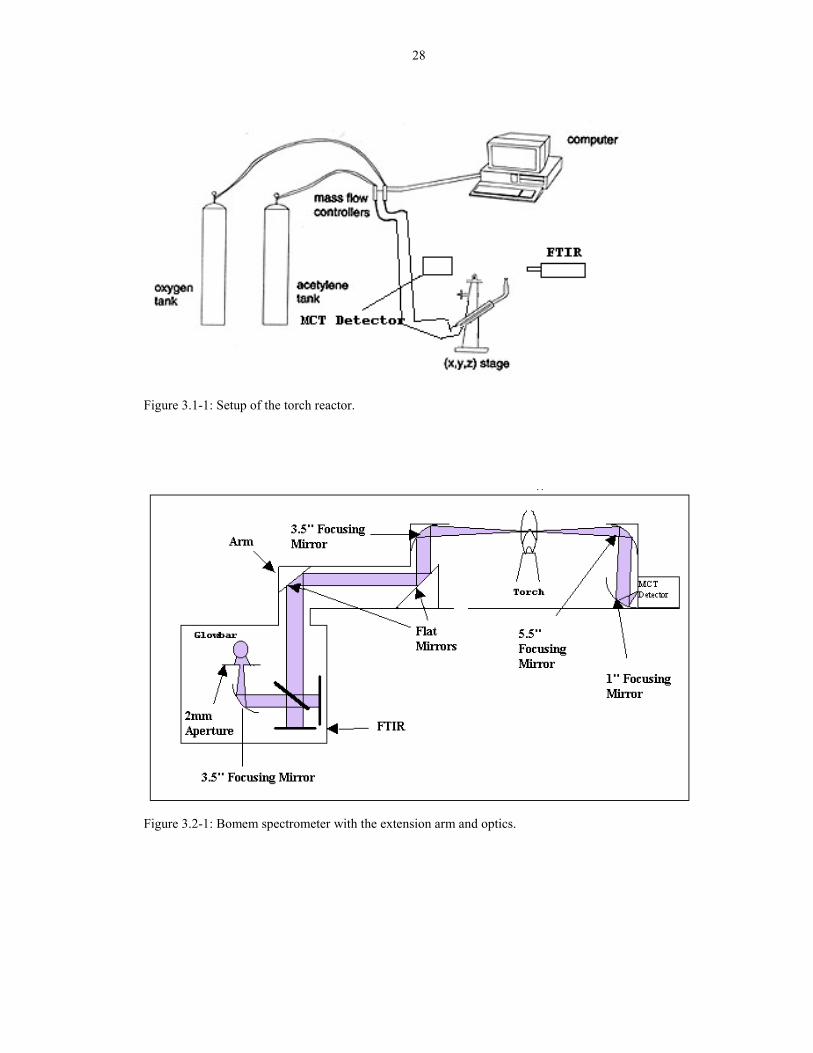
Figure 3.1-1 shows the oxyacetylene torch reactor. [1] The system is composed of

a cutting torch made by Victor with a size 0 tip positioned on an xyz translator. The 0

tip has a 1-mm diameter hole and was straightened slightly so that the inverted torch

can be used with the FTIR extension arm. The torch was pointing upward to

minimize the flicker noise in the IR spectra. (See Chapter 4 for a detailed analysis.)

The flow rate to the torch was 2L/min total. MKS Instruments Inc. makes the mass

flow controllers used to control the flow rates of acetylene and oxygen. Both

controllers are types 1259C-10000RV that have a range of 0-10 slm of N2. The mass

flow controllers was linked to a computer using Labview software (National

Instruments). The software controlled the R ratio while depositing diamond films.

A telescope made by Specell Model M820-S with a 1/20-mm scale was used to

measure the distance between the inner cone and the substrate in addition to

measuring the width of the flame.

3.2 Spectrometer

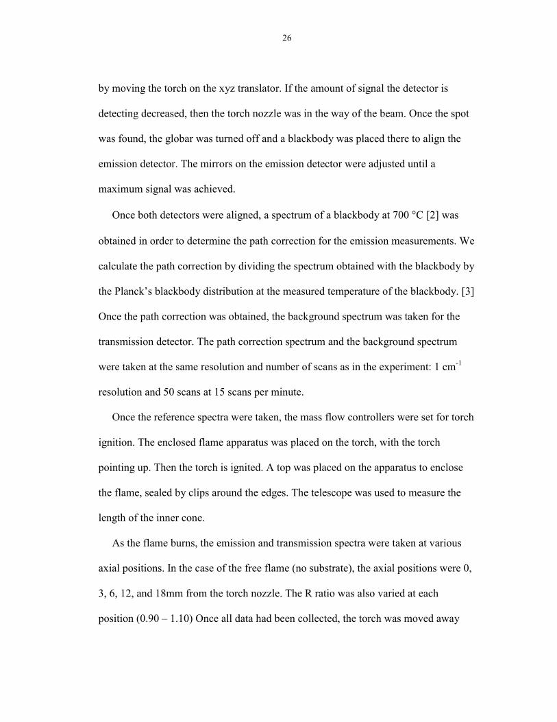
The FTIR spectrometer used for this experiment is a Bomem model MB157 with a

maximum resolution of 1cm-1 (See Figure 3.0-1 and 3.0-2). The range of sensitivity is

500 cm-1 to 6500 cm-1. The spectrometer has an internal globar that is similar to a

blackbody at 1300K. A 2 mm aperture was placed in front of the globar to reduce the

spot size and gain spatial resolution. The globar is capable of obtaining power from

24

an external power supply in the event that a hotter globar temperature is desired. An

emission port is available on the spectrometer for placing an MCT detector to collect

emission spectra. Two Mercury-Cadmium-Telluride (MCT) detectors, with a mid and

near IR range and cooled by liquid nitrogen, are used. All spectra are averages of fifty

scans at 15 scans per minute.

An extension arm was placed over to spectrometer to direct the beam to the flame.

Figure 3.2-1 presents a schematic drawing of the spectrometer and the arm. The beam

from the globar travels through the aperture and a 3.5� focal length mirror inside the

spectrometer. This parabolic mirror collimates the beam into the spectrometer. Then

the collimated IR beam from the spectrometer reflects from two flat gold plated

mirrors to divert and extend the beam. The beam is then sent to a parabolic mirror

with a focal length of 3.5 inches. The flame was placed at the focal point at the 3.5�

focal length mirror. Since the globar is behind a 2-mm aperture (which acts as the

limiting aperture), the globar can be viewed as a 2-mm diameter source. The first

parabolic mirror has a focal length of 3.5 inches and the parabolic mirror before the

sample also has a 3.5 inch focal length resulting in a magnification of one. Therefore,

the spot size is approximately the size of the internal globar, 2 mm in diameter.

However, due to the imperfections of the optics, the measured size was 3 mm in

diameter.

Since flickering interferes with the FTIR measurements, a longwave bandpass

filter (OCLI) was used for some experiments (see Chapter 4). Since most of the

flickering occurs in the CO and CO2 bands (2100-2400 cm-1), the filter blocks

25

wavenumbers above 2100 cm-1. This filter was placed at the entrance of the

transmission MCT detector.

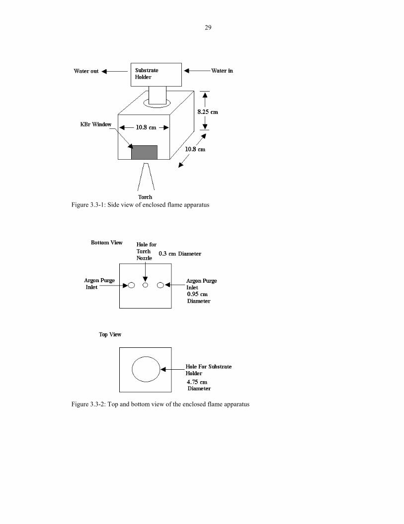
3.3 Enclosed Flame Apparatus

The drawing of the enclosing apparatus is shown in Figure 3.3-1 and 3.3-2.

Because the IR transparent KBr windows used in the apparatus cannot withstand the

high temperature (>100°C), the windows were placed away from the flame. The torch

entered the apparatus through the bottom opening. The bottom of the apparatus has

two inlets for argon purge. The Ar flow of 6 slm purges the combustible gases from

inside the apparatus. The hot gases flow out of the apparatus through an opening on

top of the apparatus. The exit area (about 1.5 square inches) must be small enough to

prevent oxygen from backflowing into the apparatus.

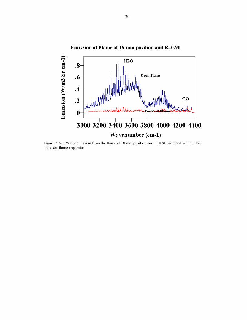
Since the outer flame indicates the presence of entrained air, the apparatus was

tested to see if the outer flame was eliminated. Figure 3.3-3 shows the spectrum of the

flame at the water band with and without the enclosure. The enclosure was quite

effective in shielding the flame.

3.4 Operational Procedure

Before starting any experimental work, the MCT detectors were cooled by liquid

nitrogen for 15 minutes. In the meantime, the IR source to the FTIR was turned on

and the transmission detector was aligned, using the alignment feature on the

Bomem/Grams 386 software. The location of the spot (focal point) was determined

26

by moving the torch on the xyz translator. If the amount of signal the detector is

detecting decreased, then the torch nozzle was in the way of the beam. Once the spot

was found, the globar was turned off and a blackbody was placed there to align the

emission detector. The mirrors on the emission detector were adjusted until a

maximum signal was achieved.

Once both detectors were aligned, a spectrum of a blackbody at 700 °C [2] was

obtained in order to determine the path correction for the emission measurements. We

calculate the path correction by dividing the spectrum obtained with the blackbody by

the Planck�s blackbody distribution at the measured temperature of the blackbody. [3]

Once the path correction was obtained, the background spectrum was taken for the

transmission detector. The path correction spectrum and the background spectrum

were taken at the same resolution and number of scans as in the experiment: 1 cm-1

resolution and 50 scans at 15 scans per minute.

Once the reference spectra were taken, the mass flow controllers were set for torch

ignition. The enclosed flame apparatus was placed on the torch, with the torch

pointing up. Then the torch is ignited. A top was placed on the apparatus to enclose

the flame, sealed by clips around the edges. The telescope was used to measure the

length of the inner cone.

As the flame burns, the emission and transmission spectra were taken at various

axial positions. In the case of the free flame (no substrate), the axial positions were 0,

3, 6, 12, and 18mm from the torch nozzle. The R ratio was also varied at each

position (0.90 � 1.10) Once all data had been collected, the torch was moved away

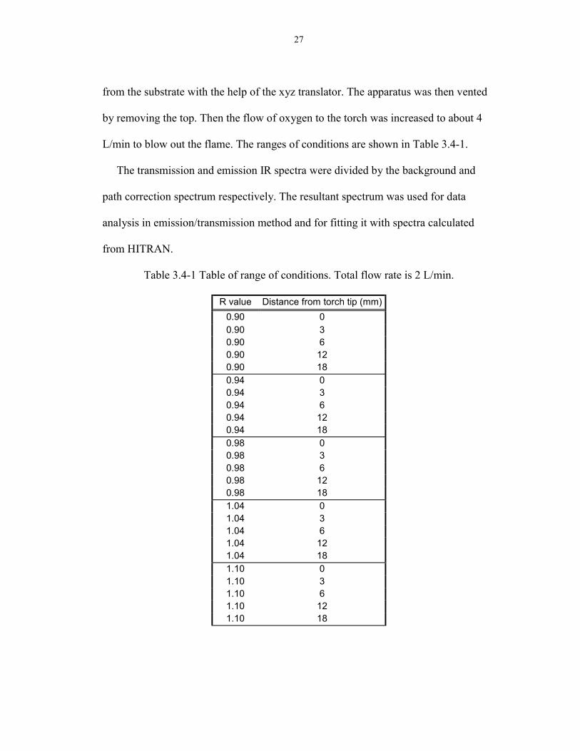
27

from the substrate with the help of the xyz translator. The apparatus was then vented

by removing the top. Then the flow of oxygen to the torch was increased to about 4

L/min to blow out the flame. The ranges of conditions are shown in Table 3.4-1.

The transmission and emission IR spectra were divided by the background and

path correction spectrum respectively. The resultant spectrum was used for data

analysis in emission/transmission method and for fitting it with spectra calculated

from HITRAN.

Table 3.4-1 Table of range of conditions. Total flow rate is 2 L/min.

R value Distance from torch tip (mm)0.90 00.90 30.90 60.90 120.90 180.94 00.94 30.94 60.94 120.94 180.98 00.98 30.98 60.98 120.98 181.04 01.04 31.04 61.04 121.04 181.10 01.10 31.10 61.10 121.10 18

28

Figure 3.1-1: Setup of the torch reactor.

Figure 3.2-1: Bomem spectrometer with the extension arm and optics.

29

Figure 3.3-1: Side view of enclosed flame apparatus

Figure 3.3-2: Top and bottom view of the enclosed flame apparatus

30

Figure 3.3-3: Water emission from the flame at 18 mm position and R=0.90 with and without theenclosed flame apparatus.

31

4.0 METHODS TO ELIMINATE FLAME NOISE

4.1 Problem Statement

The FTIR expects to detect just the modulated frequencies produced by the

interferometer (Chapter Two). For the spectrometer used for this experiment, the

Fourier frequency range lies between 105 � 1400 Hz (corresponding to 500 cm-1 to

6500 cm-1). However, the hot oxyacetylene flame also emits fluctuating IR radiation

inside the range 0-500 Hz that interferes with the FTIR measurements. Therefore, a

high level of noise is introduced to the infrared spectrum. Researchers postulate that

the source of modulation (flicker) is a combination of turbulence, combustion

instabilities, and buoyancy of the hot gases. Flicker may also result from the

combustion reactions occurring simultaneously at the exit of the torch. As more

reactions occur simultaneously, the amount of heat produce and the concentrations of

the species vary. Since the rates of reactions are determined by the concentration, the

reaction rates vary also. Therefore, the system never quite reaches equilibrium. Elfeky

et al. [1] studied turbulent flames and suggested that the flames become noisy because

of combustion instabilities. They suggested that the noise is associated with

irregularities of the flame front and speed. The flame flicker is then the fluctuation of

the amount of emitting species, pressure, or other characteristics of the flame front

due to flow pulsation. Even though the flames used in our experiments were mainly

laminar [2], these radiation fluctuations can still be present due to the combustion

reactions occurring in the inner cone of the flame. It was observed that as the

equivalence ratio increases (R decreasing), the amplitude of oscillation increased. [1]

32

They observed that lean limit of flammability was governed by low frequency

oscillations (less than 30 Hz) and fuel rich conditions were governed frequencies

greater than 30 Hz (30Hz corresponds to about 140 cm-1 on the Bomem MB151

spectrometer). Since it is necessary to be slightly fuel rich when depositing diamond,

it is expected that higher frequencies will be observed in the oxyacetylene flame.

Due to the fluctuating IR from the flame, the transmission interferograms taken

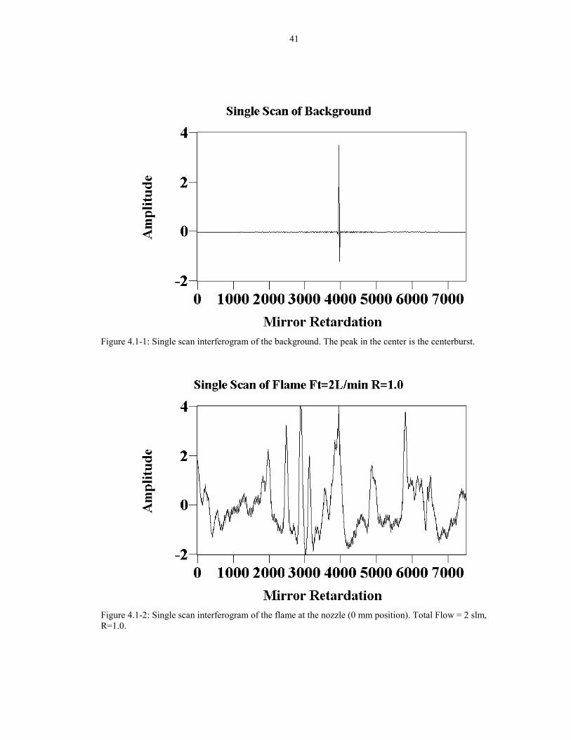
through the flame have extra noise. Figure 4.1-1 shows an interferogram of a

background spectrum (no flame present). The centerburst is clearly seen in the

middle, at about 3900 x-units with the wings of the interferogram quickly falling to

some very low value. In contrast, an interferogram taken through the flame is shown

in Figure 4.1-2. Note that the centerburst is very hard to see due to the noise of the

flame. Furthermore, the flicker intensity is the same magnitude as the centerburst.

The frequency of the noise in the flame can be determined by measuring the

flicker with the globar off and converting the �interferogram� to a power spectrum.

Since each wavenumber has a distinct modulation frequency for a particular

spectrometer, the detector detects these frequencies which is then Fourier transformed

to intensity vs. frequency. (Since the frequency is proportional to wavenumber

(Equation 2.5-4), intensity vs wavenumber is directly related to intensity vs.

frequency). The power spectrum is nothing more than a complex Fourier transform of

the noise interferogram, yielding a plot of amplitude vs. frequency. We then plot

amplitude vs frequency as amplitude vs. wavenumbers to identify where the noise

peaks appear in a flame spectrum. Any noise signal that shows up below 500 cm-1 is

33

clearly noise since the detector cannot detect below 500 cm-1. Therefore, a peak that

appeared at 300 cm-1 is from the torch emitting IR modulated at a low frequency that

corresponded to 300 cm-1 for the MB157 spectrometer. The modulation frequency of

the flame can then be calculated knowing the conversion between frequency and

wavenumber for the particular spectrometer. The spectrometer used in this

experiment has the 7225 cm-1 modulated at 1500 Hz. This was calculated by putting a

chopper in between a blackbody and a transmission detector. The chopper was

modulating the blackbody signal at 1500 Hz and a peak at 7225 cm-1 was observed in

the spectrum.

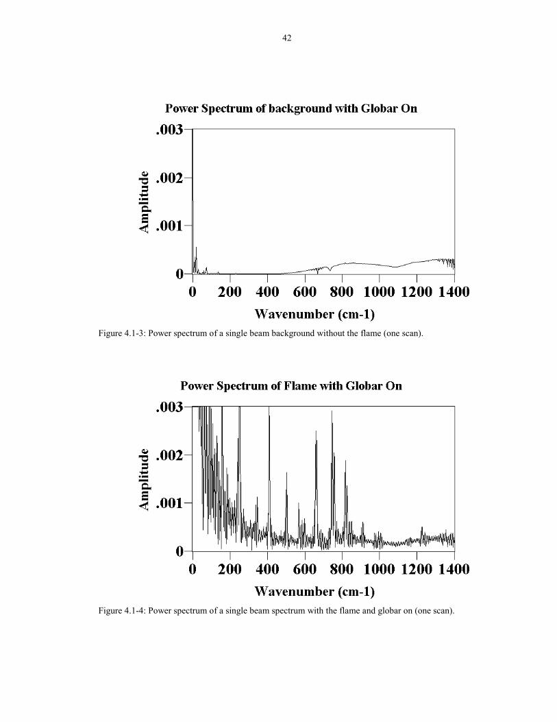
The power spectrum of the background (globar on) in Figure 4.1-3 shows that

there is very little amplitude below 500 cm-1. The power spectrum of a single scan

through the flame with the globar on is shown in Figures 4.1-4 (low wavenumber)

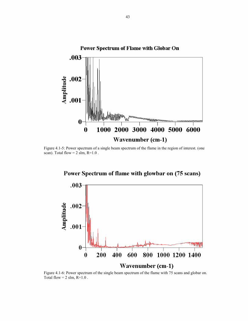
and 4.1-5 (full spectrum). The two figures show that there are many noise spikes at

low wavenumbers (frequencies), and the spikes can be more than one hundred times

the globar intensity. This means that the flame was heavily modulated at low

frequencies, interfering with the low wavenumber FTIR measurements. In addition,

the flicker raised the noise generally throughout the entire spectrum. If the modulated

IR signal emitting from the flame was purely random noise, it should signal average

away with multiple scans. The power spectrum of the same flame with 75 scans (5

minutes) shows that the frequency had been reduced significantly (See Figure 4.1-6),

but the low wavenumber region is still contaminated with the flicker noise. The

reason for this arises because the signal to noise ratio is proportional to the square

34

root of the number of scans, and the flicker noise level is large compared to the FTIR

signal. If the noise is about 100 times the FTIR signal, it would take 10,000 scans to

reduce the noise to the intensity level of the globar. At one cm-1 resolution, this would

take about 11 hours.

In summary, the low wavenumber region is most effected by the flame flickering.

This is due to the flame emission modulating at low frequencies, which lie within the

range of the modulated frequency for the FTIR used for this experiment. Since a lot

of useful information is in the low wavenumber regions, we have investigated several

ways to minimize the flicker noise

4.2 Methods to Eliminate Flame Noise

Several techniques have been investigated to reduce the flicker noise. These

include using a two detector configuration, pointing the flame upward, using

apertures, blocking the CO and CO2 absorption, and using a long-pass infrared filter.

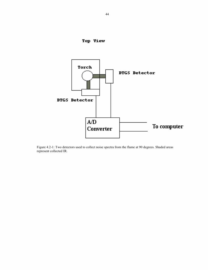
4.2.1 Two detector configuration

The idea here was to use two detectors for data acquisition, one to detect noise and

the other to detect signal plus noise. If both detectors saw the same flicker noise, then

subtracting the two interferograms should result in a flicker free interferogram. To

test that idea, two detectors were used to collect noise from the flame at positions 90

degrees from each other. (Figure 4.2-1) The same FTIR powered both detectors, and

an A/D converter (Model AT-AO-10 with the software Labview 4.0 by National

Instruments) collected voltage data from the two DTGS detectors. Prior to

35

measurements on the flame, the two detector system was tested using a light bulb as a

modulated IR source. The two spectra collected from the two detectors overlapped.

When used to measure the flame, however, the two �flickering intererograms�

collected from the two detectors do not exactly match. (Figures 4.2-2 and 4.2-3) If the

noises were identical, then a spectra subtraction of the two noise spectra should yield

zero. However, that is not the case as shown in Figure 4.2-4.

In summary, the noise in the flame is not symmetric since the noise at 90° from

each other was different. In addition, the noise generated by the flame is very random,

so the two noise �interferograms� detected at different times were also different.

Therefore, the double detector configuration will not work.

4.2.2 Pointing the flame upward

When pointing the flame upward, we observed that the noise level decreased

significantly. As hot gases exit the nozzle, buoyant forces give the gases a tendency to

travel upward. If the torch tip was pointing downward, the hot gases exiting the

nozzle flow downward while buoyancy drives them upward. This causes disturbance

in the gases resulting in oscillations. Figure 4.2-5 shows the single scan of the flame

pointing downward. The signal to noise ratio (SNR) for this interferogram is about

6.8. In contrast, the single scan of the flame pointing upward is shown in Figure 4.2-

6. The SNR for this interferogram is about 76, which is about 11 times better than the

flame pointing down. The power spectra for the flickering �interferograms� (globar

off) are shown in Figure 4.2-7 and 4.2-8 respectively. The amplitude of the noise is

generally less with the torch pointing up than down. The dominant frequencies are

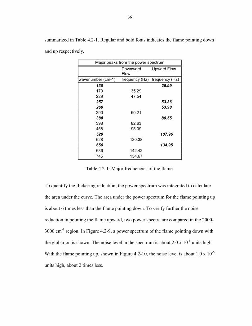
36

summarized in Table 4.2-1. Regular and bold fonts indicates the flame pointing down

and up respectively.

Major peaks from the power spectrumDownwardFlow

Upward Flow

wavenumber (cm-1) frequency (Hz) frequency (Hz)130 26.99170 35.29229 47.54257 53.36260 53.98290 60.21388 80.55398 82.63458 95.09520 107.96628 130.38650 134.95686 142.42745 154.67

Table 4.2-1: Major frequencies of the flame.

To quantify the flickering reduction, the power spectrum was integrated to calculate

the area under the curve. The area under the power spectrum for the flame pointing up

is about 6 times less than the flame pointing down. To verify further the noise

reduction in pointing the flame upward, two power spectra are compared in the 2000-

3000 cm-1 region. In Figure 4.2-9, a power spectrum of the flame pointing down with

the globar on is shown. The noise level in the spectrum is about 2.0 x 10-5 units high.

With the flame pointing up, shown in Figure 4.2-10, the noise level is about 1.0 x 10-5

units high, about 2 times less.

37

Another scenario to examine related to buoyancy driven flicker is the amount of

flicker noise introduced by placing the substrate in the flame. The power spectrum of

a single scan flame pointing up without the substrate is shown in Figure 4.2-11 and

4.2-13. The power spectrum of a single scan flame with the substrate is shown in

Figures 4.2-12 and 4.2-14. The spectra without the substrate have lower amplitude

noise in the low frequency region (ie. low wavenumbers) compared to the one with

the substrate. However, at higher frequencies, the one with the substrate is slightly

better. This means that the substrate is causing more low frequency flicker and less

high frequency flicker.

In summary, it is more advantageous to take FTIR spectra of the flame pointing

up. The amplitude of the flicker at all frequencies is generally lower with the flame

pointing up than it is down. In addition, when the substrate is placed over the flame to

deposit diamond, the low frequency flickering was increased while the higher

frequency noises were decreased.

4.2.3 Apertures

Another method to reduce the flicker noise was to place an aperture between the

flame and the transmission detector. The objective is to screen out flicker that may be

collected by the detector optics with as little impact as possible on the FTIR signal.

To study the effect of the SNR with apertures, apertures of different sizes were placed

in the path of the IR between the flame and the transmission detector with the flame

pointing up. The aperture was adjusted to see which size would yield the best SNR.

The signal is taken to be the height of the centerburst in the interferogram and the

38

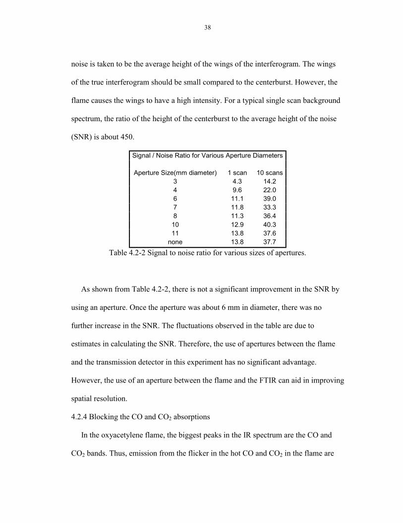
noise is taken to be the average height of the wings of the interferogram. The wings

of the true interferogram should be small compared to the centerburst. However, the

flame causes the wings to have a high intensity. For a typical single scan background

spectrum, the ratio of the height of the centerburst to the average height of the noise

(SNR) is about 450.

Signal / Noise Ratio for Various Aperture Diameters

Aperture Size(mm diameter) 1 scan 10 scans3 4.3 14.24 9.6 22.06 11.1 39.07 11.8 33.38 11.3 36.410 12.9 40.311 13.8 37.6

none 13.8 37.7Table 4.2-2 Signal to noise ratio for various sizes of apertures.

As shown from Table 4.2-2, there is not a significant improvement in the SNR by

using an aperture. Once the aperture was about 6 mm in diameter, there was no

further increase in the SNR. The fluctuations observed in the table are due to

estimates in calculating the SNR. Therefore, the use of apertures between the flame

and the transmission detector in this experiment has no significant advantage.

However, the use of an aperture between the flame and the FTIR can aid in improving

spatial resolution.

4.2.4 Blocking the CO and CO2 absorptions

In the oxyacetylene flame, the biggest peaks in the IR spectrum are the CO and

CO2 bands. Thus, emission from the flicker in the hot CO and CO2 in the flame are

39

largely responsible for the modulated signal. Therefore, if a bag of CO or CO2 is

placed between the flame and the detector, the bag absorbes most of the CO and CO2

emission from the flame, thereby reducing the noise level to the rest of the spectrum.

However, the bag needs to be optically thick, so the major disadvantage of this is that

all the CO and CO2 information is lost.

For comparison, Figure 4.2-15 shows the power spectrum of the flicker noise

from the flame going through an empty polyethylene bag. The power spectrum of the

same bag filled with CO is shown in Figure 4.2-16. As shown in the figures, the CO

in the bag was not very efficient in minimizing the noise in the power spectrum. The

spectra here were taken with the DTGS detector instead of the MCT detector. Notice

that the flickering frequencies are much higher than the ones with MCT (Figure 4.2-

11) because the DTGS detector is much slower than the MCT detector. Therefore, the

flickering frequencies appear higher when using the DTGS detector.

Similarly, the power spectra of the flicker noise from the flame (globar on)

without the bag and the bag filled with CO2 is shown in Figures 4.2-17 and 4.2-18

respectively. The spikes in the power spectrum have drastically decreased. The

polyethylene bag has not decreased the amount of noise in the spectrum because if it

did, the same trend would be observed in the CO bag experiment. Therefore, it must

be the CO2 in the bag that has decreased the flicker noise received by the detector.

In summary, the CO2 bag is much more efficient in reducing the spikes and noise

in the spectra, especially in the 500-6500 cm-1 region. Thus, methods to filter out the

IR emission from CO2 can also reduce the flicker noise.

40

4.2.5 Long-pass infrared filters

The use of an infrared long-pass filter should also achieve the same effect as the

CO2 bag. A long-pass infrared filter ( Optical Coatings Laboratory Inc.) is designed

to filter out everything above 2100 cm-1, and this can remove the dominant CO and

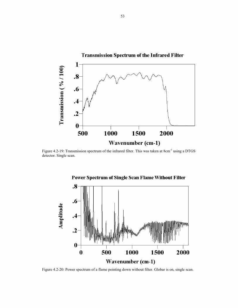
CO2 emission from the flame. The transmission spectrum of the filter is shown in

Figure 4.2-19. Therefore, spectra taken with the filter can be used to obtain low

wavenumber (less than 2100 cm-1) data, and the spectra taken without the filter can be

used to analyze regions above 2100cm-1 (where flicker noise is unimportant).

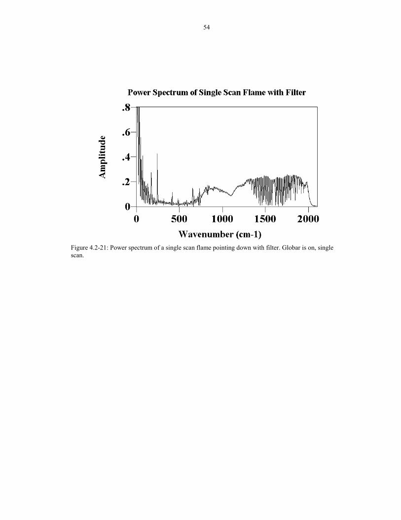
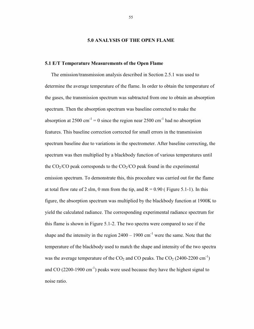
In order to prove this point, a power spectrum was again analyzed for both cases,

with and without the filter (Figures 4.2-20 and 4.2-21). As shown, the noise spikes are

greatly reduced as well as the general noise level (see regions near 1000 cm-1). The

peak-to-peak value is approximately .0061 for the case with the filter and is about

0.013 for the case without the filter. The peak-to-peak value is the amplitude of noise

in the 1200 cm-1 region of the spectrum. The noise level decreased by a factor of two

with the use of a filter.

In summary, two methods have worked well in minimizing the flame noise:

pointing the flame up and the use of an infrared filter. Both methods reduced the

general noise level. These two methods should allow for an increased in SNR in the

low wavenumber region. Therefore, both methods were incorporated in obtaining

data in this experiment.

41

Figure 4.1-1: Single scan interferogram of the background. The peak in the center is the centerburst.

Figure 4.1-2: Single scan interferogram of the flame at the nozzle (0 mm position). Total Flow = 2 slm,R=1.0.

42

Figure 4.1-3: Power spectrum of a single beam background without the flame (one scan).

Figure 4.1-4: Power spectrum of a single beam spectrum with the flame and globar on (one scan).

43

Figure 4.1-5: Power spectrum of a single beam spectrum of the flame in the region of interest. (onescan). Total flow = 2 slm, R=1.0 .

Figure 4.1-6: Power spectrum of the single beam spectrum of the flame with 75 scans and globar on.Total flow = 2 slm, R=1.0 .

44

Figure 4.2-1: Two detectors used to collect noise spectra from the flame at 90 degrees. Shaded areasrepresent collected IR.

45

Figure 4.2-2: Flame noise detected by first DTGS detector at 0° using Labview for data acquisition.

Figure 4.2-3: DTGS detector at 90° from the first one using Labview for data acquisition.

Figure 4.2-4: Subtraction of the two spectra obtain from detectors at 90° from each other.

46

Figure 4.2-5: Interferogram of the flame pointing down. Flame is at 2 slm total flow, R=0.94, at the tipof the torch. Single scan. Globar on.

Figure 4.2-6: Interferogram of the flame pointing up. Flame is at 2 slm total flow, R=0.94 at the tip ofthe torch. Single scan with globar on.

47

Figure 4.2-7: Power spectrum of the flame pointing down and globar off. Flame is at 2 slm total flow,R=0.94, and at the tip of the torch. Single scan.

Figure 4.2-8: Power spectrum of the flame pointing up with globar off. Flame is at 2 slm total flow,R=0.94, and at the tip of the torch. Single scan.

48

Figure 4.2-9: Power spectrum of single scan flame pointing down and globar on in the 2000-3000 cm-1

region. Flame is at 2 slm total flow, R=0.94, and at the tip of the torch. Single scan.

Figure 4.2-10: Power spectrum of single scan flame pointing up with globar on. Flame is at 2 slm totalflow, R=0.94, and at the tip of the torch. Single scan.

49

Figure 4.2-11: Power spectrum of single scan flame without substrate.

Figure 4.2-12: Power spectrum of single scan flame with substrate in 0 � 2000 cm-1 region.

50

Figure 4.2-13: Power spectrum of flame without substrate in 2000 � 4000 cm-1 region.

Figure 4.2-14: Power spectrum of single scan flame with substrate in 2000 � 4000 cm-1 region.

51

Figure 4.2-15: Power spectrum of an equivalent single scan of flame noise with a polyethylene bagusing a DTGS detector. Globar was off.

Figure 4.2-16: Power spectrum of equivalent single scan of flame noise with CO in bag using a DTGSdetector. Globar off.

52

Figure 4.2-17: Power spectrum of the single scan flame without polyethylene bag and globar on. Flameis pointing down.

Figure 4.2-18: Power spectrum of single scan flame with polyethylene bag filled with CO2 and globaron. Flame is pointing down.

53

Figure 4.2-19: Transmission spectrum of the infrared filter. This was taken at 8cm-1 using a DTGSdetector. Single scan.

Figure 4.2-20: Power spectrum of a flame pointing down without filter. Globar is on, single scan.

54

Figure 4.2-21: Power spectrum of a single scan flame pointing down with filter. Globar is on, singlescan.

55

5.0 ANALYSIS OF THE OPEN FLAME

5.1 E/T Temperature Measurements of the Open Flame

The emission/transmission analysis described in Section 2.5.1 was used to

determine the average temperature of the flame. In order to obtain the temperature of

the gases, the transmission spectrum was subtracted from one to obtain an absorption

spectrum. Then the absorption spectrum was baseline corrected to make the

absorption at 2500 cm-1 = 0 since the region near 2500 cm-1 had no absorption

features. This baseline correction corrected for small errors in the transmission

spectrum baseline due to variations in the spectrometer. After baseline correcting, the

spectrum was then multiplied by a blackbody function of various temperatures until

the CO2/CO peak corresponds to the CO2/CO peak found in the experimental

emission spectrum. To demonstrate this, this procedure was carried out for the flame

at total flow rate of 2 slm, 0 mm from the tip, and R = 0.90 ( Figure 5.1-1). In this

figure, the absorption spectrum was multiplied by the blackbody function at 1900K to

yield the calculated radiance. The corresponding experimental radiance spectrum for

this flame is shown in Figure 5.1-2. The two spectra were compared to see if the

shape and the intensity in the region 2400 � 1900 cm-1 were the same. Note that the

temperature of the blackbody used to match the shape and intensity of the two spectra

was the average temperature of the CO2 and CO peaks. The CO2 (2400-2200 cm-1)

and CO (2200-1900 cm-1) peaks were used because they have the highest signal to

noise ratio.

56

The water cannot be analyzed using the emission/transmission method because

there was a significant amount of water in the background. In addition, the

background level of water fluctuated, making it very hard to distinguish between

room temperature and high temperature water in the transmission spectrum. This

produced the inverted peaks in the transmission spectrum (negative peaks in the

calculated radiance of Figure 5.1-1). Therefore, the water temperature was

determined using the emission spectrum only (see below).

Using the E/T method, we had determined the average flame temperature for

different positions and R ratios in the flame (total flow rate = 2 slm). Table 5.1-1

shows the results. As shown in the table, the E/T temperature is about 1900K in the

CO band and about 1850K in the CO2 band.

From the E/T analysis, we observe that the average temperature is not a function

of position and is independent of R. The average temperature does not vary by more

than 100°C. The E/T temperature is an average because both the emission and

transmission are collected along a line of sight, so the cold portions of the flame pulls

down the radiance while increasing the absorption (1 - transmittance). Thus, the

observed E/T temperature is some average of the maximum temperature and room

temperature. Therefore, the maximum temperature (highest temperature of the

species) in the flame was used in the HITRAN analysis of concentration.

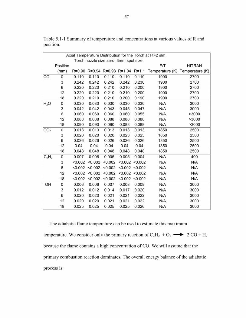
57

Table 5.1-1 Summary of temperature and concentrations at various values of R andposition.

Axial Temperature Distribution for the Torch at Ft=2 slmTorch nozzle size zero. 3mm spot size.

Position E/T HITRAN(mm) R=0.90 R=0.94 R=0.98 R=1.04 R=1.1 Temperature (K) Temperature (K)

CO 0 0.110 0.110 0.110 0.110 0.110 1900 27003 0.242 0.242 0.242 0.242 0.230 1900 27006 0.220 0.220 0.210 0.210 0.200 1900 270012 0.220 0.220 0.210 0.210 0.200 1900 270018 0.220 0.210 0.210 0.200 0.190 1900 2700

H2O 0 0.030 0.030 0.030 0.030 0.030 N/A 30003 0.042 0.042 0.043 0.045 0.047 N/A 30006 0.060 0.060 0.060 0.060 0.055 N/A >300012 0.088 0.088 0.088 0.088 0.088 N/A >300018 0.090 0.090 0.090 0.088 0.088 N/A >3000

CO2 0 0.013 0.013 0.013 0.013 0.013 1850 25003 0.020 0.020 0.020 0.023 0.025 1850 25006 0.026 0.026 0.026 0.026 0.026 1850 250012 0.04 0.04 0.04 0.04 0.04 1850 250018 0.048 0.048 0.048 0.048 0.048 1850 2500

C2H2 0 0.007 0.006 0.005 0.005 0.004 N/A 4003 <0.002 <0.002 <0.002 <0.002 <0.002 N/A N/A6 <0.002 <0.002 <0.002 <0.002 <0.002 N/A N/A12 <0.002 <0.002 <0.002 <0.002 <0.002 N/A N/A18 <0.002 <0.002 <0.002 <0.002 <0.002 N/A N/A

OH 0 0.006 0.006 0.007 0.008 0.009 N/A 30003 0.012 0.012 0.014 0.017 0.020 N/A 30006 0.020 0.020 0.021 0.021 0.022 N/A 300012 0.020 0.020 0.021 0.021 0.022 N/A 300018 0.025 0.025 0.025 0.025 0.026 N/A 3000

The adiabatic flame temperature can be used to estimate this maximum

temperature. We consider only the primary reaction of C2H2 + O2 2 CO + H2

because the flame contains a high concentration of CO. We will assume that the

primary combustion reaction dominates. The overall energy balance of the adiabatic

process is:

58

∆H = 0 = ∆Hf (298) + ∆Hp (5.1-1)

where ∆Hf = heat of formation and ∆Hp = enthalpy change of the products. Therefore,

under adiabatic conditions, the heat of reaction must equal to the enthalpy change of

the products from room temperature to the flame temperature. If chemical equilibrium

is neglected and all the products are CO and H2, then the heat of reaction is �338 kJ.

Based on this, the adiabatic flame temperature is about 3000K. This value is similar

to the experimental temperature.

5.2 CO2 Measurements of the Open Flame

Using the temperature from the E/T analysis of the CO/CO2 bands, the CO2

emission cannot be simulated correctly. The shapes of the calculated emission

spectrum using HITRAN and HITEMP at the E/T temperature differs substantially

from the experimental emission spectrum. Figure 5.2-1 shows the hot bands present

in the experimental emission spectrum around the 2400 cm-1 region. These peaks do

not appear in flames less than 2000K. Therefore, it is not possible that the CO2 is

about 1800K, as predicted by the E/T measurements. These trends were also observed

by Scutaru et al. [1] where they found that HITRAN92 is missing many high

temperature lines below 2300 cm-1 when the temperature is above 700K. They

compared experimental radiance spectra to those calculated using HITRAN92 in the

temperature range of 750K to 2850K. Since the authors showed some spectra of

experimental vs. HITRAN calculated spectra, those empirical correlations can be

used to estimate the amount of CO2 in our flame. According to Scutaru et al. [1], the

59

HITRAN92 database did a reasonable good job at fitting the CO2 bands in the region

of 2350 � 2400 cm-1 at high temperature. In addition, they found that the HITRAN92

calculated intensity of the peaks at 2200 � 2300 cm-1 is roughly 50% of the

experimental values. Therefore, we used the region 2350 � 2400 cm-1 to fit the

experimental spectrum to the HITRAN calculated spectrum. Restricting our analysis

to that region only, we found that 0.013 atm cm of CO2 at 2500K was in the flame at

0 mm position, total flow rate of 2 slm and R=0.90 (see Figure 5.2-2).

As shown in Figure 5.2-2, the 2350 � 2400 cm-1 region fits reasonably well, and

the intensity of the calculated spectrum in the region 2200-2300 cm-1 is roughly 50%

of the experimental spectrum, which corresponds to what others have observed. [1]

Therefore, for all the other gases (CO, H2O, OH, C2H2 , CH4, CO2), the temperature

was adjusted until the shapes in the radiance fits with the calculated shapes. The

HITRAN temperature and concentrations for CO2 appear in Table 5.1-1 and Figures

5.6-8 to 5.6-12.

5.3 CO Measurements of the Open Flame

The calculated CO emission for 2700K at 0.11 atm cm is shown in Figure 5.3-1.

This spectrum matches very nicely with the CO region of the experimental emission

spectrum of the flame at 0 mm position, total flow rate of 2 slm and R=0.90 (Figure

5.2-1). By combining this with the calculated CO2 spectrum in Figure 5.2-2, the

resulting spectrum is shown in Figure 5.3-2. The comparison between this calculated

spectrum to the experimental emission spectrum is shown in Figure 5.3-3. These two

60

spectra are very close to each other except for the missing hot CO2 bands.

Concentration and temperature results for CO at other conditions appear in Table 5.1-

1 and Figures 5.6-8 to 5.6-12.

The main result found in Table 5.1-1 is that the concentrations of CO and CO2 do

not vary significantly with R ratio. For instance, consider the emission spectrum of

the flame at 0 mm position, total flow rate of 2 slm, and R=1.10 shown in Figure 5.3-

4 (Note that the neutral flame condition is at R=1.03). The two spectra of R=0.90

(Figure 5.2-1) and R=1.10 (Figure 5.3-4) do not differ very much as shown by the

subtraction of the two spectra (Figure 5.3-5). The difference is about 0.1 at max,

which is about an 8% difference. Noting the temperatures are roughly the same, this

implies that the amount of CO2 is about 8% higher when the R ratio is 1.10 compared

to 0.90. However, since the amount of CO2 in the flame is low, an 8% increase yields

0.014 atm cm for R = 1.10 vs. 0.013 atm cm for R=0.90. This increase is very small.

However, there is a definite trend that when the R ratio increases, the amount of CO2

in the flame increases.

5.4 H2O Measurements of the Open Flame

To obtain the amount of water in the flame, the emission spectra has been studied

because the transmission spectrum is contaminated with water from the background.

The amount of water in the background changes with time, making it hard to

determine the amount of water in the flame. The emission spectra are better since the

61

water vapor in the room does not emit IR whereas hot water vapor in the flame emits

significant IR.

The best place to look when analyzing the water is in the 2600 � 3100 cm-1 region

since both the H2O and OH bands are observed in that region. In addition, the

curvature of the spectrum in this region is strongly dependent on the temperature of

the water. Therefore, if the temperature of the water is correct, the shape should be

the same. This is shown in Figure 5.4-1 where the water emission is compared the

calculated (HITEMP Voigt) emission spectra at 1900K and 3000K. The experimental

emission spectrum is much closer to the 3000K spectra. Therefore, the water in the

flame should be about 3000K as shown in Figure 5.4-2. In the open free flame (Ft = 2

slm, R = 0.90 at the 0 mm position), there is ~0.03 atm cm of water. The calculated

(HITEMP) spectrum fits the observed spectrum well. The water concentration does

not vary much with R ratio at the 0 mm position. The water bands at R=0.90 and 1.10

are compared, there is no significant difference in the water emission.

Since the water is at about 3000K, there should be hot water lines in the

transmission spectrum. Even though the background spectrum is dominated by room

temperature water from the atmosphere, the hot water bands should still appear in the

transmission spectrum since hot water is much broader that room temperature water

(shown in Figure 5.4-3). (Although the partial pressure is different in the two

calculated spectra, the 0.03 atm cm of water at 3000K is equivalent to 0.003 atm cm

water at 300K since the concentration and path length is constant). Using Figure 5.4-3

62

as a guide, we can observe these hot water bands in the experimental transmission

spectrum (Figure 5.4-4).

Similar water analyses were done at different position and R value of the flame.

The results are tabulated in Table 5.1-1 and shown in Figures 5.6-8 through 5.6-12.

5.5 OH Measurements of the Open Flame

There are OH features in the spectrum as shown in Figure 5.4-1 and 5.4-2. When

trying to determine the temperature of the OH, different temperatures were compared

to the experimental spectrum until there is a good fit. When the OH is added to the

water spectrum (0.03 atm cm at 3000K), the 3000K OH spectrum fit better because

the features below 3000 cm-1 are more intense, agreeing with the experimental

spectrum. The comparison of the calculated H2O + OH spectra and the experimental

spectrum is shown in Figure 5.5-1. The difference of the two spectra is shown in

Figure 5.5-2. There is a slight difference in the baseline, with a maximum difference

of 36% and an average error of �2%. This error is considered good. Some of the

difference is that the temperature of the water is postulated to be above 3000K, but

the database used for calculation was only available up to 3000K. Note that there is

an extra line in Figure 5.5-2 (noted by an asterisk) at 3587 cm-1, which may be due to

missing data in the HITRAN database.

Similar analyses were done at other position and R values of the flame for OH.

The results are tabulated in Table 5.1-1 and shown in Figures 5.6-8 through 5.6-12.

63

5.6 C2H2 Measurements of the Open Flame

The two strongest absorption features for C2H2 are at 730 cm-1 and 3280 cm-1.

Preliminary comparisons of HITRAN calculations and experiment found that the

calculated acetylene peaks in the 730 cm-1 and 3280 cm-1 bands are not consistent

with each other. Therefore, detailed experiments were carried out to compare the

experimental and calculated acetylene spectra. A spectrum of acetylene flowing (at

0.048 atm and 300K) through a gas cell of 15 cm long was taken at 1 cm-1 resolution

and appears in Figures 5.6-1 (730 cm-1 band) and 5.6-2 (3280 cm-1 band). Notice that

the calculated spectrum at 730 m-1 is about six times higher than the experimental

spectrum (Figure 5.6-1). The Q branch (730 cm-1) shown has an absorbance of 11.5

units while the experimental spectrum shows an absorbance of 1.7 units. When

comparing the spectra at the 3280 cm-1 (Figure 5.6-2), the peaks are much more

similar in intensity and shape. Therefore, HITRAN92 and HITRAN96 over predicts

the peak at 730 cm-1 while the peak at 3280 cm-1 is more accurate. Therefore, the

peak at 3280 cm-1 was used for quantitative analysis.

The emission spectra do not show any acetylene at any R values or locations in the

flame; C2H2 is observed only in the transmission. Therefore, the temperature of the

acetylene must be low. Using the experimental transmittance alone, we find the best

fit with 0.007 atm cm at 400K. A comparison of calculation and experimental spectra

is shown in Figure 5.6-3 with the difference of the two spectra shown in Figure 5.6-4.

The average difference is 0.0006, which is very small. The average percentage error

is about 6%. Most of it is due to the noise in the transmission spectrum. Other

64

position and R values were calculated for C2H2 and are tabulated in Table 5.1-1 and

shown in Figure 5.6-8 through 5.6-12.

The temperature of the acetylene dictates the shape of its transmission spectrum.

Therefore, if the experimental shapes of the acetylene peak (at 3280 cm-1) match the

calculated shapes, then the temperature is correct. At 300K, the maxima in the P and

R branches are not at the same location as the experimental C2H2 spectrum (Figure

5.6-5). The same scenario occurs when 500K acetylene is calculated (Figure 5.6-6).

The 400K calculated spectrum matches up much better (Figure 5.6-3).

At 0 mm position, acetylene is observed for all R ratios, and as the R ratio

increases, the amount of acetylene decreases. The detection limit for acetylene is

0.002 atm cm, twice the noise level. At the 3, 6, 12, and 18 mm positions, the level of

acetylene is below the detection limit.

If acetylene is present in the flame, the acetylene peak at 730 cm-1 should also

appear in the transmission spectrum. This peak is observed in the transmission

spectrum using the longpass infrared filter to reduce the flicker noise (Figure 5.6-7).

However, the calculated 730 cm-1 peak is bigger than the experimental, in line with

experiments with the acetylene gas cell.

5.7 Discussion of Results

In the following discussion, we assume that the species observed with the FTIR in

this experiment are produced by the following four reactions:

C2H2 + O2 2 CO + H2 (5.7-1)H2 + ½ O2 H2O (5.7-2)

65

2CO + O2 2 CO2 (5.7-3)H2+ O2 2OH (5.7-4)

Equation 5.7-1 is the primary combustion step while the other reactions account for

secondary combustion processes. Now consider the following analysis for the data at

0 mm position and R = 0.90. Since 0.013 atm cm of CO2 is produced, there is 0.013

atm cm of CO converted to CO2 due to the 1:1 stoichiometry of Equation 5.7-1.

Combined with measured CO, that means at least 0.123 atm cm of CO is produced in

the primary combustion. From stoichiometry, that means at least 0.062 atm cm of H2

is produced in the primary reaction (Equation 5.7-1). However, the amount of H2 can

be higher if some of the C2H2 converts directly to C or C2, which are not detectable

by the FTIR. Since there are 0.03 atm cm of H2O present in the flame, at least 0.032

atm cm of H2 (or 0.064 atm cm of hydrogen radicals) is in the flame. Similar analysis

for H2 at other positions and R values appears in Table 5.7-1.

Since we know how much CO and CO2 is in the flame, it is also possible to

determine how much C2H2 is consumed by the reactions. Based on the first reaction,

there should be about 0.0615 atm cm of C2H2 consumed to produce 0.123 atm cm of

CO. With a residual 0.007 atm cm at 400K, the corrected concentration is (assuming

the CO and CO2 are at 2500K in the flame):

5218.)300(300400007.0

30025000615.0 22 ==+ KHC atm cm (5.7-5)

where C2H2 (300K) is the equivalent amount of C2H2 entering the flame at a

temperature of 300K. If the amount of oxygen / acetylene ratio is 0.90, then the

amount of oxygen fed to the torch is about 0.47 atm cm 300K and 0.056 atm cm at

66

2500K. The oxygen entrainment is the difference between the amount of oxygen

needed to produce the observed CO, OH, CO2, and H2O, and the amount fed to the

torch. There should be about 0.086 atm cm necessary to produce the observed CO,

OH, CO2, and H2O in the flame. This leads to an oxygen entrainment of 0.03 atm cm

(2500K) at the 0 mm position. Since the oxygen entrainment comes from the air,

there would be nitrogen in the flame that is not detectable by the FTIR. The nitrogen

entrainment is calculated based on the air containing 79% nitrogen and 21 % oxygen.

Value for different positions and R values are tabulated in Table 5.7-1. Note that the

values there have the units of atm cm. Therefore, if the path length of each individual

gases were known, then those values can be divided by its path length to yield partial

pressure. Unfortunately, the path lengths are unknown, but some general trends are

still clear (Figure 5.6-13 to 5.6-14).

Note that the O2 diffusion is greater when it is farther from the nozzle. This makes

very good intuitive sense since more oxygen will entrain the flame farther along the

flow axis. There is a big jump between the 0 and 3 mm position because of the great

concentration difference there. Based on the way the O2 entrainment is calculated, if

this position contains a high level of C and C2 radicals that the FTIR cannot detect, it

lowers the calculated amount of oxygen fed to the torch, thereby increasing the O2

entrainment.

The amount of H2 is highest at the 3 mm position, which is the region in which

diamond growth occurs. When the flow rate is 2 slm, the inner cone is about 4 mm in

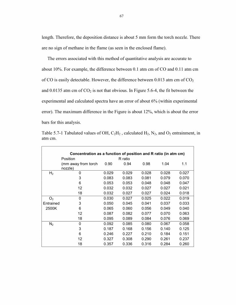
67

length. Therefore, the deposition distance is about 5 mm form the torch nozzle. There

are no sign of methane in the flame (as seen in the enclosed flame).

The errors associated with this method of quantitative analysis are accurate to

about 10%. For example, the difference between 0.1 atm cm of CO and 0.11 atm cm

of CO is easily detectable. However, the difference between 0.013 atm cm of CO2

and 0.0135 atm cm of CO2 is not that obvious. In Figure 5.6-4, the fit between the

experimental and calculated spectra have an error of about 6% (within experimental

error). The maximum difference in the Figure is about 12%, which is about the error

bars for this analysis.

Table 5.7-1 Tabulated values of OH, C2H2 , calculated H2, N2, and O2 entrainment, inatm cm.

Concentration as a function of position and R ratio (in atm cm)Position R ratio(mm away from torchnozzle)

0.90 0.94 0.98 1.04 1.1

H2 0 0.029 0.029 0.028 0.028 0.0273 0.083 0.083 0.081 0.079 0.0706 0.053 0.053 0.048 0.048 0.04712 0.032 0.032 0.027 0.027 0.02118 0.032 0.027 0.027 0.024 0.018

O2 0 0.030 0.027 0.025 0.022 0.019Entrained 3 0.050 0.045 0.041 0.037 0.033

2500K 6 0.065 0.060 0.056 0.049 0.04012 0.087 0.082 0.077 0.070 0.06318 0.095 0.089 0.084 0.076 0.069

N2 0 0.092 0.085 0.080 0.067 0.0583 0.187 0.168 0.156 0.140 0.1256 0.246 0.227 0.210 0.184 0.15112 0.327 0.308 0.290 0.261 0.23718 0.357 0.336 0.316 0.284 0.260

68

In summary, we found that different species have slightly different temperature

because they are located in different parts of the flame. The major trends is that the

concentration of CO2, H2O, and O2 entrained increases with increasing axial position.

The amount of C2H2 decreases with increasing axial position, and CO and H2 have a

maximum at position 3 mm from the torch nozzle. There is also a big jump in the

partial pressure * pathlength at the 3 mm position. These results are shown in Figures

5.6-8 to 5.6-14.

As the R ratio increases, the amount of CO is about constant at the 0 mm position

and it decreases at positions greater than 0 mm. For the H2O, the amount is constant

at 0 mm position, increases at the 3 mm position, then decreases at the 6 mm position,

and finally levels off at positions greater than 12 mm. For the CO2, as R increases, the

amount of CO2 remains constant at all positions except for the 3 mm, where it

increases. For the C2H2 , the amount decreases with increasing R ratio. For OH, the

amount increases with increasing R ratio. Finally for the H2 and O2 entrainment, the

amount decreases with increasing R ratio.

5.8 Comparison of Results to Previous Work

Morrison et al. [2, 3] performed in situ measurements of the oxyacetylene flame

with the FTIR. The most extensive data set is the radial profiles of concentration and

temperature at 9 mm from the torch nozzle. They found that the temperature of the

flame is about 3000K at the tip of the torch, consistent with HITRAN temperature

here. Since the temperature reported in this experiment is the average temperature

69

over a 3 mm spot size, then the temperatures reported by Morrison et al. must be

average over the first 3 mm in order to draw a correct comparison. If the temperature

in the first 3 mm is averaged, the temperature is very close. However, they did report

a decrease in relative concentration of the CO species farther from the flame, which is

again consistent with what is observed here. The authors did not observe any

acetylene in the flame.

Matsui et al. [4, 5] observed CH* and C2* by emission spectroscopy in the inner

cone which were not observed in this experiment. However, C2* is not observable by

the FTIR, and the concentration of CH* may be too low to be detected using the FTIR

under the noisy flame. They estimated partial pressure of CH as 2 x 10-5 to 6 x 10-5

atm. [6] These concentrations are too low to be measured. Matsui et al. also observed

OH in the flame at the outer boundary. The results in this experiment are consistent

with that since we quantitatively showed OH is in higher amounts farther from the

inner cone.

Yalamanchi et al. [7] found C, CH, and H in the inner cone. Again, the C and H

are not observable by the FTIR and the concentration of CH may be too low to be

detected (the authors did not report on the concentration of CH).

Matsui et al. [8] found high concentration of CO and H2 in the feather region of

the flame at R = 0.90. This is also consistent with results presented here in this

experiment, where high concentration of CO is found in the feather region (3mm

from torch tip) (Table 5.1-1 and Figures 5.6-8 to 5.6-12 and Figure 5.6-14). The

authors also found water and acetylene at lower levels than CO and H2 in the flame.

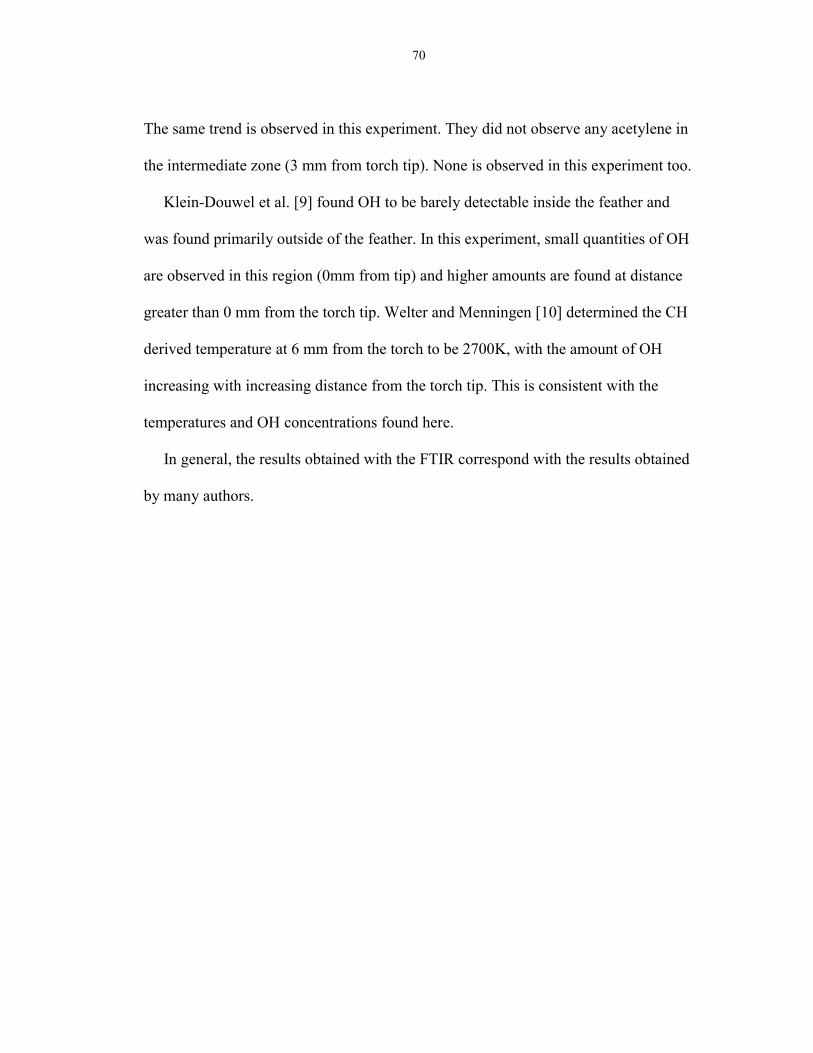
70

The same trend is observed in this experiment. They did not observe any acetylene in

the intermediate zone (3 mm from torch tip). None is observed in this experiment too.

Klein-Douwel et al. [9] found OH to be barely detectable inside the feather and

was found primarily outside of the feather. In this experiment, small quantities of OH

are observed in this region (0mm from tip) and higher amounts are found at distance

greater than 0 mm from the torch tip. Welter and Menningen [10] determined the CH

derived temperature at 6 mm from the torch to be 2700K, with the amount of OH

increasing with increasing distance from the torch tip. This is consistent with the

temperatures and OH concentrations found here.

In general, the results obtained with the FTIR correspond with the results obtained

by many authors.

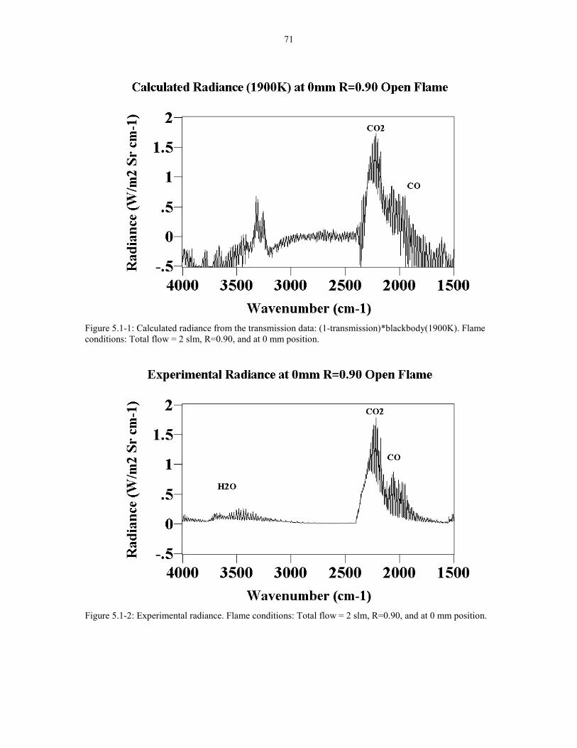
71

Figure 5.1-1: Calculated radiance from the transmission data: (1-transmission)*blackbody(1900K). Flameconditions: Total flow = 2 slm, R=0.90, and at 0 mm position.

Figure 5.1-2: Experimental radiance. Flame conditions: Total flow = 2 slm, R=0.90, and at 0 mm position.

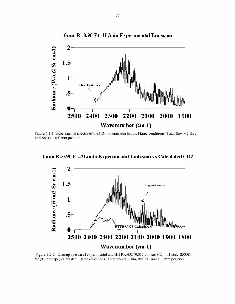
72

Figure 5.2-1: Experimental spectra of the CO2 hot emission bands. Flame conditions: Total flow = 2 slm,R=0.90, and at 0 mm position.

Figure 5.2-2: Overlap spectra of experimental and HITRAN92 (0.013 atm cm CO2 in 1 atm, 2500K;Voigt lineshape) calculated. Flame conditions: Total flow = 2 slm, R=0.90, and at 0 mm position.

73

Figure 5.3-1: Calculated spectrum from HITRAN96 with 0.11 atm cm in 1 atm at 2700K; Voigt lineshape.

Figure 5.3-2: Combined spectra of calculated CO (0.11 atm cm in 1 atm, 2700K, HITRAN96 Voigtlineshape) and CO2 (0.013 atm cm 2500K, HITRAN92 Voigt lineshape).

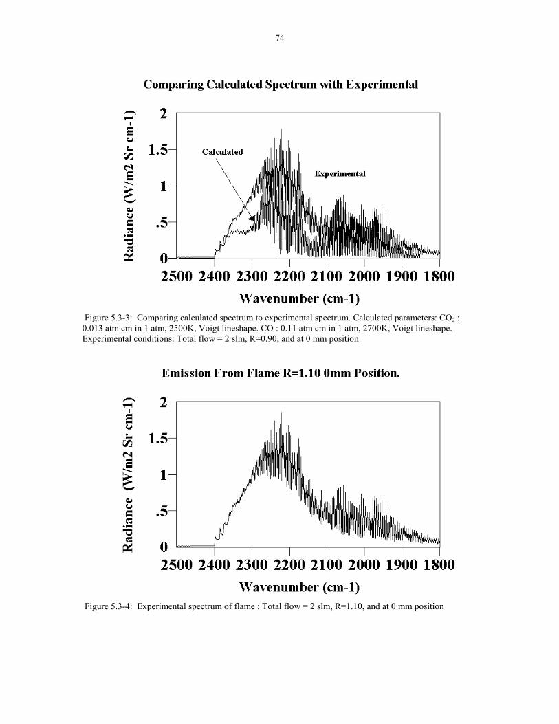
74

Figure 5.3-3: Comparing calculated spectrum to experimental spectrum. Calculated parameters: CO2 :0.013 atm cm in 1 atm, 2500K, Voigt lineshape. CO : 0.11 atm cm in 1 atm, 2700K, Voigt lineshape.Experimental conditions: Total flow = 2 slm, R=0.90, and at 0 mm position

Figure 5.3-4: Experimental spectrum of flame : Total flow = 2 slm, R=1.10, and at 0 mm position

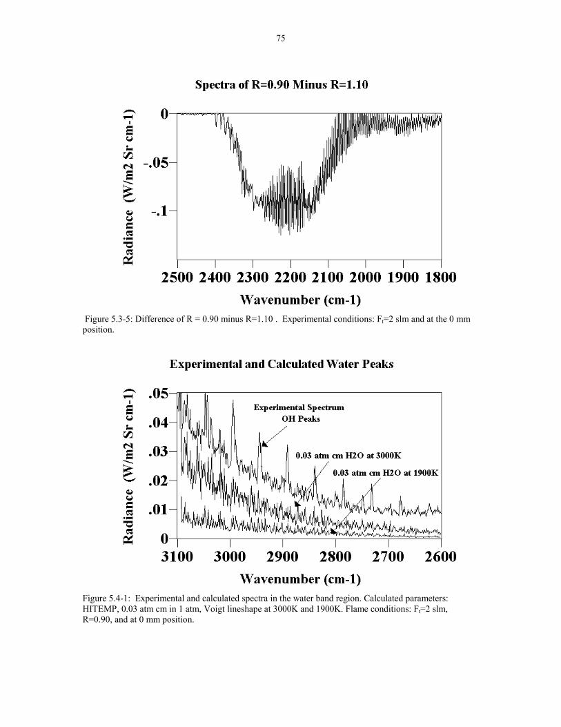
75

Figure 5.3-5: Difference of R = 0.90 minus R=1.10 . Experimental conditions: Ft=2 slm and at the 0 mmposition.

Figure 5.4-1: Experimental and calculated spectra in the water band region. Calculated parameters:HITEMP, 0.03 atm cm in 1 atm, Voigt lineshape at 3000K and 1900K. Flame conditions: Ft=2 slm,R=0.90, and at 0 mm position.

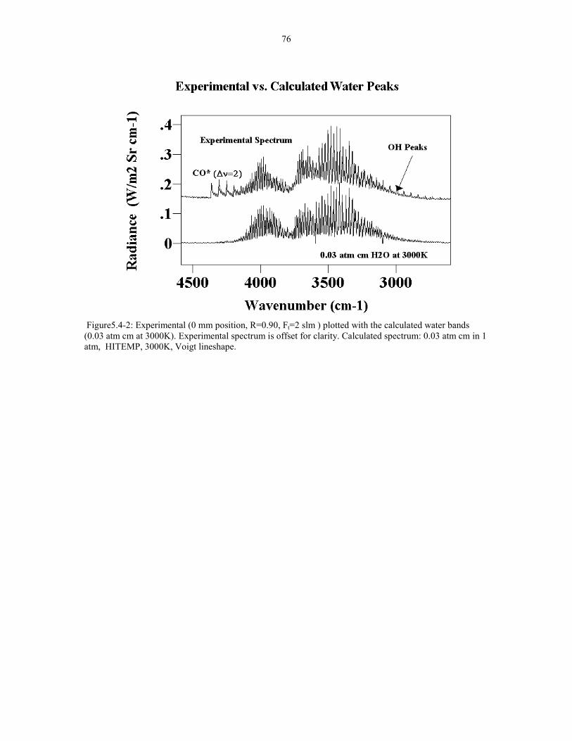
76

Figure5.4-2: Experimental (0 mm position, R=0.90, Ft=2 slm ) plotted with the calculated water bands(0.03 atm cm at 3000K). Experimental spectrum is offset for clarity. Calculated spectrum: 0.03 atm cm in 1atm, HITEMP, 3000K, Voigt lineshape.

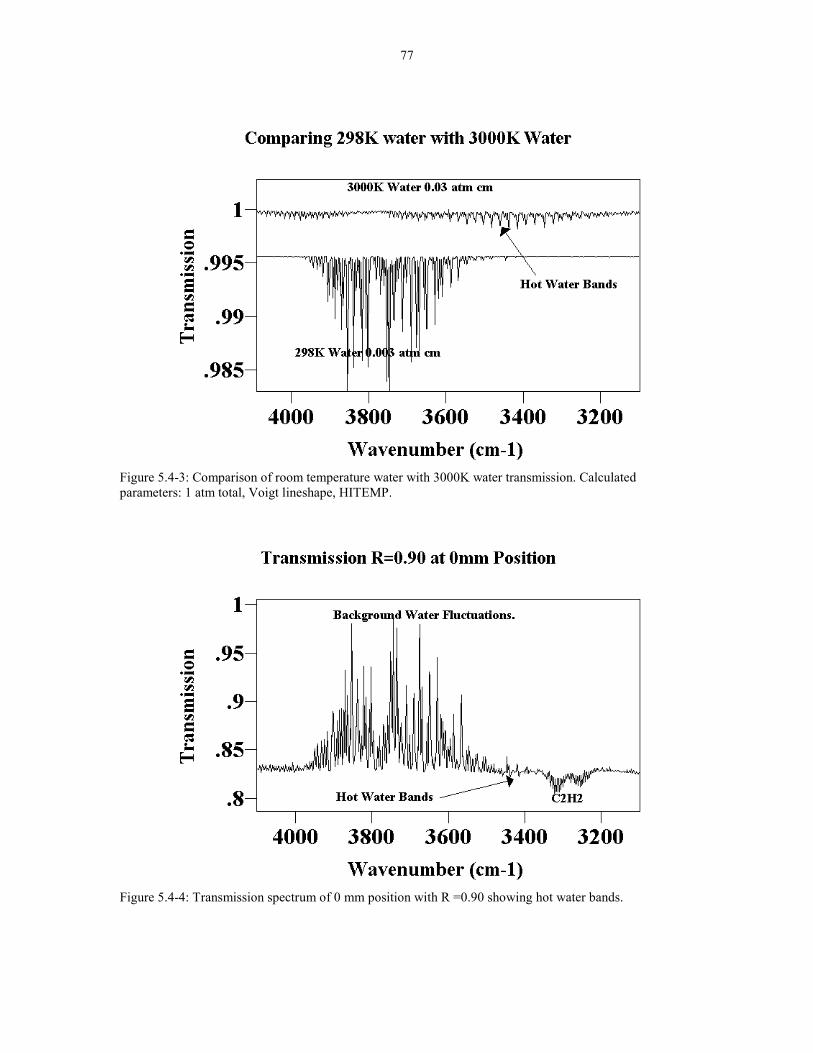
77

Figure 5.4-3: Comparison of room temperature water with 3000K water transmission. Calculatedparameters: 1 atm total, Voigt lineshape, HITEMP.

Figure 5.4-4: Transmission spectrum of 0 mm position with R =0.90 showing hot water bands.

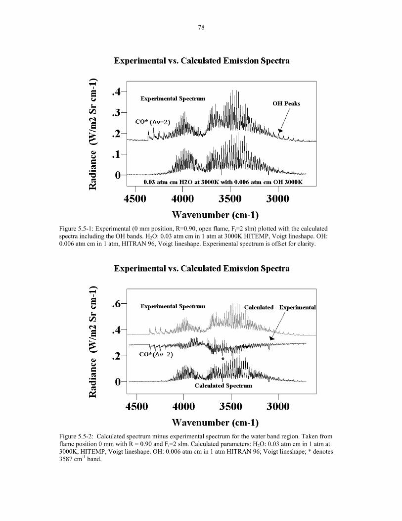
78

Figure 5.5-1: Experimental (0 mm position, R=0.90, open flame, Ft=2 slm) plotted with the calculatedspectra including the OH bands. H2O: 0.03 atm cm in 1 atm at 3000K HITEMP, Voigt lineshape. OH:0.006 atm cm in 1 atm, HITRAN 96, Voigt lineshape. Experimental spectrum is offset for clarity.

Figure 5.5-2: Calculated spectrum minus experimental spectrum for the water band region. Taken fromflame position 0 mm with R = 0.90 and Ft=2 slm. Calculated parameters: H2O: 0.03 atm cm in 1 atm at3000K, HITEMP, Voigt lineshape. OH: 0.006 atm cm in 1 atm HITRAN 96; Voigt lineshape; * denotes3587 cm-1 band.

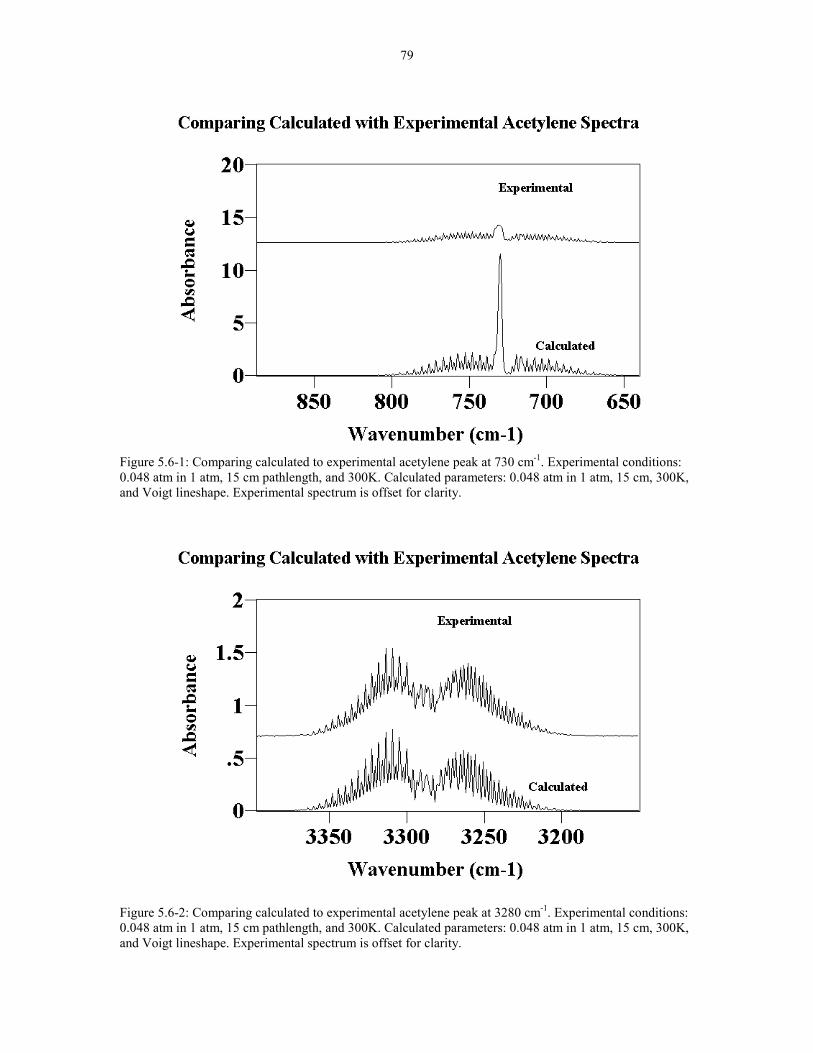
79

Figure 5.6-1: Comparing calculated to experimental acetylene peak at 730 cm-1. Experimental conditions:0.048 atm in 1 atm, 15 cm pathlength, and 300K. Calculated parameters: 0.048 atm in 1 atm, 15 cm, 300K,and Voigt lineshape. Experimental spectrum is offset for clarity.

Figure 5.6-2: Comparing calculated to experimental acetylene peak at 3280 cm-1. Experimental conditions:0.048 atm in 1 atm, 15 cm pathlength, and 300K. Calculated parameters: 0.048 atm in 1 atm, 15 cm, 300K,and Voigt lineshape. Experimental spectrum is offset for clarity.

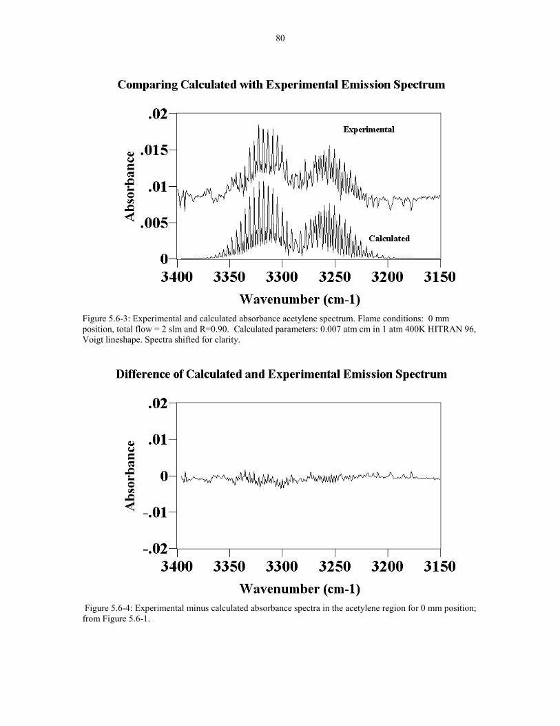
80

Figure 5.6-3: Experimental and calculated absorbance acetylene spectrum. Flame conditions: 0 mmposition, total flow = 2 slm and R=0.90. Calculated parameters: 0.007 atm cm in 1 atm 400K HITRAN 96,Voigt lineshape. Spectra shifted for clarity.

Figure 5.6-4: Experimental minus calculated absorbance spectra in the acetylene region for 0 mm position;from Figure 5.6-1.

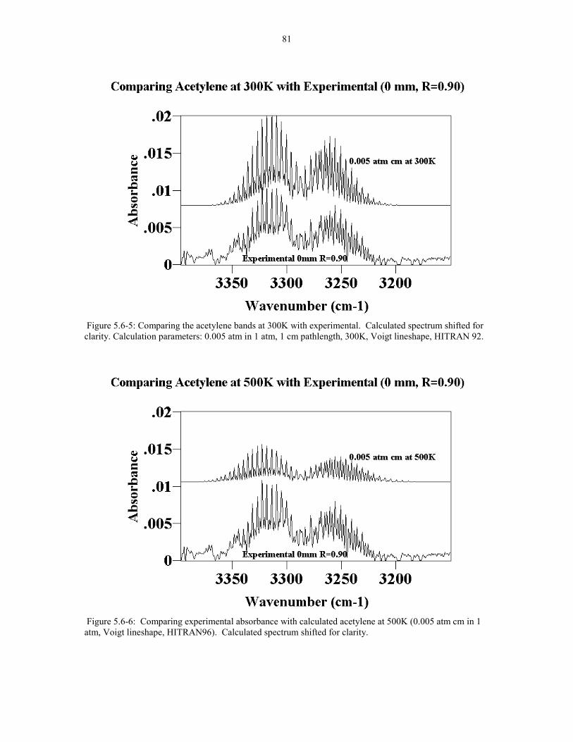
81

Figure 5.6-5: Comparing the acetylene bands at 300K with experimental. Calculated spectrum shifted forclarity. Calculation parameters: 0.005 atm in 1 atm, 1 cm pathlength, 300K, Voigt lineshape, HITRAN 92.

Figure 5.6-6: Comparing experimental absorbance with calculated acetylene at 500K (0.005 atm cm in 1atm, Voigt lineshape, HITRAN96). Calculated spectrum shifted for clarity.

82

Figure 5.6-7: Comparing calculated acetylene spectrum (400K) with experimental spectrum (0 mmposition and R=0.90) in the 730cm-1 region.

Free Open Flame R = 0.90

0.000

0.010

0.020

0.030

0.040

0.050

0.060

0.070

0.080

0.090

0.100

0 5 10 15 20

Distance from Torch (mm)

Part

ial P

ress

ure

* Pat

h le

ngth

(atm

cm

)

0.000

0.050

0.100

0.150

0.200

0.250

0.300

CO

con

cent

ratio

n (a

tm c

m)

H2OCO2C2H2OHCO

Figure 5.6-8: Plot of concentrations as a function of distance for R=0.90 Ft=2 slm.

83

Open free flame R=0.94

0.000

0.010

0.020

0.030

0.040

0.050

0.060

0.070

0.080

0.090

0.100

0 5 10 15 20

Distance from torch (mm)

Part

ial P

ress

ure

* Pat

h le

ngth

(atm

cm

)

0.000

0.050

0.100

0.150

0.200

0.250

0.300

CO

con

cent

ratio

n (a

tm c

m)

H2O

CO2

C2H2

OH

CO

Figure 5.6-9: Plot of concentration as a function of distance at R=0.94 Ft=2 slm

Figure 5.6-10: Plot of concentration versus distance for R=0.98

Open free flame R=0.98

0.000

0.020

0.040

0.060

0.080

0.100

0 5 10 15 20Distance from torch (mm)

Part

ial P

ress

ure

* Pat

h le

ngth

(a

tm c

m)

0.000

0.050

0.100

0.150

0.200

0.250

0.300C

O c

once

ntra

tion

(atm

cm

)

H2OCO2C2H2OHCO

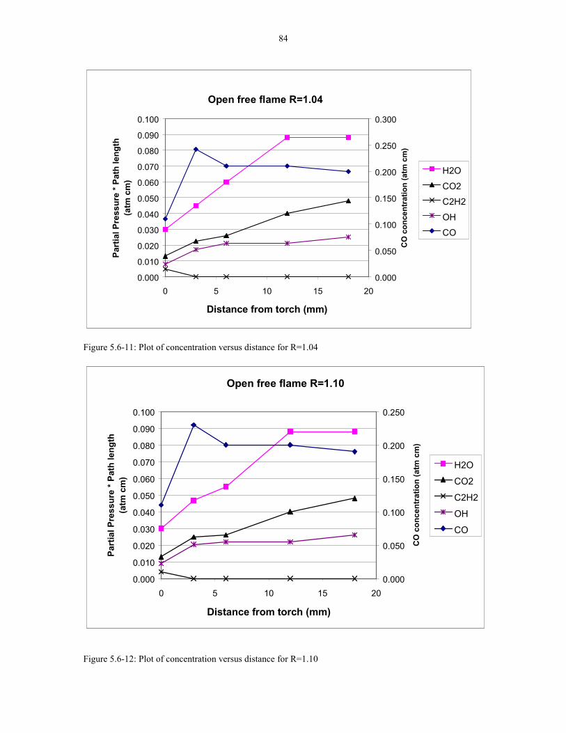
84

Open free flame R=1.04

0.000

0.010

0.020

0.030

0.040

0.050

0.060

0.070

0.080

0.090

0.100

0 5 10 15 20

Distance from torch (mm)

Part

ial P

ress

ure

* Pat

h le

ngth

(a

tm c

m)

0.000

0.050

0.100

0.150

0.200

0.250

0.300

CO

con

cent

ratio

n (a

tm c

m)

H2O

CO2C2H2

OHCO

Figure 5.6-11: Plot of concentration versus distance for R=1.04

Open free flame R=1.10

0.000

0.010

0.020

0.030

0.040

0.050

0.060

0.070

0.080

0.090

0.100

0 5 10 15 20

Distance from torch (mm)

Part

ial P

ress

ure

* Pat

h le

ngth

(a

tm c

m)

0.000

0.050

0.100

0.150

0.200

0.250C

O c

once

ntra

tion

(atm

cm

)

H2O

CO2

C2H2

OH

CO

Figure 5.6-12: Plot of concentration versus distance for R=1.10

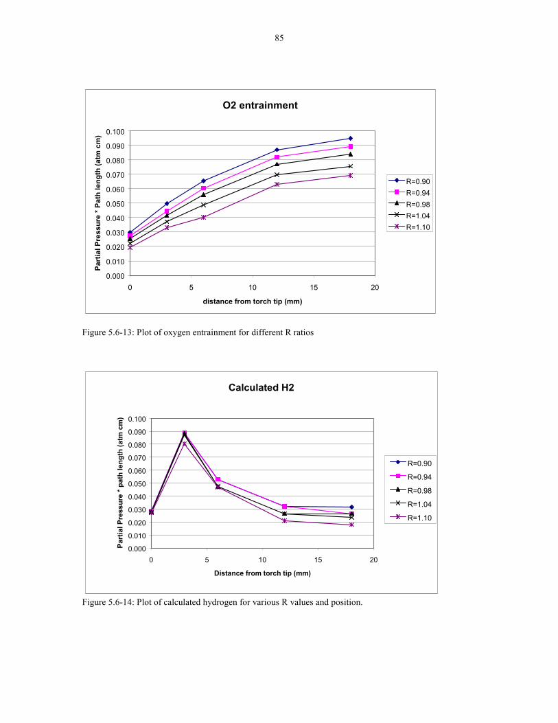
85

O2 entrainment

0.000

0.010

0.020

0.030

0.040

0.050

0.060

0.070

0.080

0.090

0.100

0 5 10 15 20

distance from torch tip (mm)

Part

ial P

ress

ure

* Pat

h le

ngth

(atm

cm

)

R=0.90R=0.94R=0.98R=1.04R=1.10

Figure 5.6-13: Plot of oxygen entrainment for different R ratios

Calculated H2

0.000

0.010

0.020

0.030

0.040

0.050

0.060

0.070

0.080

0.090

0.100

0 5 10 15 20

Distance from torch tip (mm)

Part

ial P

ress

ure

* pat

h le

ngth

(atm

cm

)

R=0.90

R=0.94

R=0.98

R=1.04

R=1.10

Figure 5.6-14: Plot of calculated hydrogen for various R values and position.

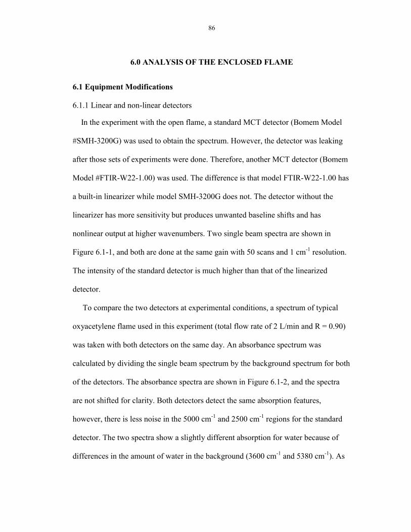
86

6.0 ANALYSIS OF THE ENCLOSED FLAME

6.1 Equipment Modifications

6.1.1 Linear and non-linear detectors

In the experiment with the open flame, a standard MCT detector (Bomem Model

#SMH-3200G) was used to obtain the spectrum. However, the detector was leaking

after those sets of experiments were done. Therefore, another MCT detector (Bomem

Model #FTIR-W22-1.00) was used. The difference is that model FTIR-W22-1.00 has

a built-in linearizer while model SMH-3200G does not. The detector without the

linearizer has more sensitivity but produces unwanted baseline shifts and has

nonlinear output at higher wavenumbers. Two single beam spectra are shown in

Figure 6.1-1, and both are done at the same gain with 50 scans and 1 cm-1 resolution.

The intensity of the standard detector is much higher than that of the linearized

detector.

To compare the two detectors at experimental conditions, a spectrum of typical

oxyacetylene flame used in this experiment (total flow rate of 2 L/min and R = 0.90)

was taken with both detectors on the same day. An absorbance spectrum was

calculated by dividing the single beam spectrum by the background spectrum for both

of the detectors. The absorbance spectra are shown in Figure 6.1-2, and the spectra

are not shifted for clarity. Both detectors detect the same absorption features,

however, there is less noise in the 5000 cm-1 and 2500 cm-1 regions for the standard

detector. The two spectra show a slightly different absorption for water because of

differences in the amount of water in the background (3600 cm-1 and 5380 cm-1). As

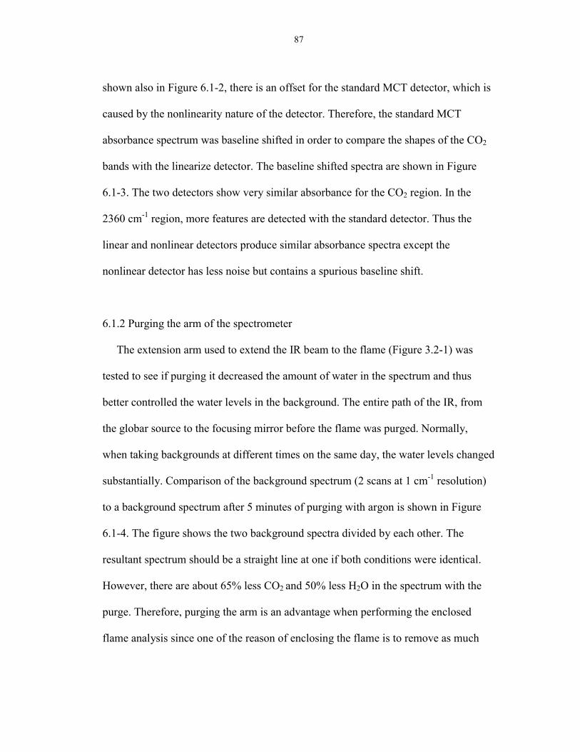
87

shown also in Figure 6.1-2, there is an offset for the standard MCT detector, which is

caused by the nonlinearity nature of the detector. Therefore, the standard MCT

absorbance spectrum was baseline shifted in order to compare the shapes of the CO2

bands with the linearize detector. The baseline shifted spectra are shown in Figure

6.1-3. The two detectors show very similar absorbance for the CO2 region. In the

2360 cm-1 region, more features are detected with the standard detector. Thus the

linear and nonlinear detectors produce similar absorbance spectra except the

nonlinear detector has less noise but contains a spurious baseline shift.

6.1.2 Purging the arm of the spectrometer

The extension arm used to extend the IR beam to the flame (Figure 3.2-1) was

tested to see if purging it decreased the amount of water in the spectrum and thus

better controlled the water levels in the background. The entire path of the IR, from

the globar source to the focusing mirror before the flame was purged. Normally,

when taking backgrounds at different times on the same day, the water levels changed

substantially. Comparison of the background spectrum (2 scans at 1 cm-1 resolution)

to a background spectrum after 5 minutes of purging with argon is shown in Figure

6.1-4. The figure shows the two background spectra divided by each other. The

resultant spectrum should be a straight line at one if both conditions were identical.

However, there are about 65% less CO2 and 50% less H2O in the spectrum with the

purge. Therefore, purging the arm is an advantage when performing the enclosed

flame analysis since one of the reason of enclosing the flame is to remove as much

88

water as possible from the spectrum. Another method to remove the water from the

spectrum was to use a desiccant in the arm. However, the desiccant did not perform

as well as purging the arm.

Therefore, the arm of the spectrometer was purged with ultra high purity nitrogen

(instead of argon because of availability) at 99.999% purity. The enclosed flame

apparatus was purged with ultra high purity argon (99.999%) to keep the KBr

windows cool and to remove the combustible gases that builds up inside.

6.2 Temperature Measurement in the Enclosed Flame

The enclosed flame has particles at the 0 mm position. This is observed in the

emission spectrum where all the gas emission features are �riding� on a greybody

shape at about 450K as seen in Figure 6.2-1. The particles are also observed in the

transmission spectrum where the entire transmission spectrum is baseline shifted from

one (Figure 6.2-2). The shift in the transmission spectrum is caused by the particles

blocking some of the light by scattering and absorption. The greybody shape seen in

Figure 6.2-1 is calculated by taking (1 � transmission) of Figure 6.2-2 and

multiplying it with a blackbody at 450K. At positions 3 mm and greater, the particles

disappeared because the transmission spectra do not show a baseline shift. This is

shown in the emission spectrum of Figure 6.2-3 where the emission spectrum does

not show a �hump� at the low wavenumber region. The transmission spectrum

(Figure 6.2-4) also shows a baseline value of 1.

89

To calculate the gas temperature by E/T, the blackbody emissions due to the

particle was subtracted from the emission spectrum before further analysis. Then the

emission baseline was shifted to zero if necessary. Then the transmission spectrum

was converted to absorbance, and the baseline due to the particles was removed.

Afterward, the spectrum was converted back to the transmission spectrum. Then, the

E/T analysis was done on the enclosed flame just like the open flames to determine

the average temperature of the CO2 and CO bands. For the water, the temperature was

determined by observing the 2100 � 2600 cm-1 region for curvature in the radiance

spectra as describe in the open free flame section. The results are tabulated in Table

6.2-1.

The temperature of the CO2 is much lower than all the other species when using

the E/T method. One reason for this is that the CO2 may be closer to the edge of the

flame. In addition, the CO temperature obtained is much cooler than that of the open

free flame because of the CO being trapped inside the enclosed flame apparatus.

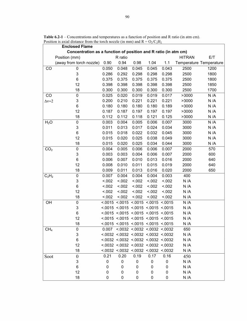
90

Table 6.2-1 � Concentrations and temperatures as a function of position and R ratio (in atm cm).Position is axial distance from the torch nozzle (in mm) and R = O2/C2H2

Enclosed FlameConcentration as a function of position and R ratio (in atm cm)

Position (mm) R ratio HITRAN E/T(away from torch nozzle) 0.90 0.94 0.98 1.04 1.1 Temperature Temperature

CO 0 0.050 0.048 0.045 0.045 0.043 2500 12003 0.286 0.292 0.298 0.298 0.298 2500 18006 0.375 0.375 0.375 0.375 0.375 2500 180012 0.398 0.398 0.398 0.398 0.398 2500 185018 0.300 0.300 0.300 0.300 0.300 2500 1700

CO 0 0.025 0.020 0.019 0.019 0.017 >3000 N /A∆ν=2 3 0.200 0.210 0.221 0.221 0.221 >3000 N /A

6 0.180 0.180 0.180 0.180 0.189 >3000 N /A12 0.187 0.187 0.197 0.197 0.197 >3000 N /A18 0.112 0.112 0.118 0.121 0.125 >3000 N /A

H2O 0 0.003 0.004 0.005 0.006 0.007 3000 N /A3 0.011 0.013 0.017 0.024 0.034 3000 N /A6 0.015 0.018 0.022 0.032 0.045 3000 N /A12 0.015 0.020 0.025 0.038 0.049 3000 N /A18 0.015 0.020 0.025 0.034 0.044 3000 N /A

CO2 0 0.004 0.005 0.006 0.006 0.007 2000 5703 0.003 0.003 0.004 0.006 0.007 2000 6006 0.006 0.007 0.010 0.013 0.016 2000 64012 0.008 0.010 0.011 0.015 0.019 2000 64018 0.009 0.011 0.013 0.016 0.020 2000 650

C2H2 0 0.007 0.004 0.004 0.004 0.003 4003 <.002 <.002 <.002 <.002 <.002 N /A6 <.002 <.002 <.002 <.002 <.002 N /A12 <.002 <.002 <.002 <.002 <.002 N /A18 <.002 <.002 <.002 <.002 <.002 N /A

OH 0 <.0015 <.0015 <.0015 <.0015 <.0015 N /A3 <.0015 <.0015 <.0015 <.0015 <.0015 N /A6 <.0015 <.0015 <.0015 <.0015 <.0015 N /A12 <.0015 <.0015 <.0015 <.0015 <.0015 N /A18 <.0015 <.0015 <.0015 <.0015 <.0015 N /A

CH4 0 0.007 <.0032 <.0032 <.0032 <.0032 6503 <.0032 <.0032 <.0032 <.0032 <.0032 N /A6 <.0032 <.0032 <.0032 <.0032 <.0032 N /A12 <.0032 <.0032 <.0032 <.0032 <.0032 N /A18 <.0032 <.0032 <.0032 <.0032 <.0032 N /A

Soot 0 0.21 0.20 0.19 0.17 0.16 4503 0 0 0 0 0 N /A6 0 0 0 0 0 N /A12 0 0 0 0 0 N /A18 0 0 0 0 0 N /A

91

6.3 CO Measurements in the Enclosed Flame

It is difficult to quantitatively analyze the CO2 and CO in an enclosed flame

because much of the CO is trapped inside the box. A large cold band of CO is

observed in the transmission spectrum: CO builds up in the box and obscures the CO

spectrum. Thus, the cold CO band absorbs some of the emission from the hot CO in

the flame as shown in Figure 6.3-1. Therefore, in order to get the concentration of the

CO in the flame, only the hot band edge from the emission spectrum was analyzed.

These hot bands are outside of the cold band in the transmission spectrum in regions

between 1900 � 2000 cm-1. The temperature determined by E/T analysis (1200K)

does not match the temperature of the CO needed to match the emission spectrum

because E/T gives average temperature, which includes the CO outside the flame.

These are shown in Figures 6.3-2 and 6.3-3. In Figure 6.3-3, it is shown that 1200K

CO does not fit the emission CO bands very well. Part of the reason again is the E/T

gives average temperature of the CO in the line of sight. If there are colder CO in the

enclosed flame apparatus, it lowered the �apparent� temperature of the CO.

The CO temperature in the flame is much closer to 2500K with a concentration of

0.05 atm cm at the 0 mm position when R = 0.90 (Figures 6.3-4). Similar analyses are

done at other positions and R values of the enclosed flame. The results are tabulated

in Table 6.2-1.

92

6.4 CO2 Measurements in the Enclosed Flame

The temperature of the CO2 has the same problem as with CO when performing

the E/T analysis. From E/T analysis, the CO2 should be about 600K. However, when

CO2 is at 600K, it does not have the hot features shown in experimental emission

spectrum (Figure 6.4-1). Those hot bands do not appear until it is above 2000K.

Therefore, this is the approximate temperature of the CO2 in the flame. Again, some

lines of the hot CO2 are missing as discussed in the open flame section (Section 5.2).

The same procedures used in the open flame analysis were used for the enclosed

flame to determine the concentration of CO2 at other axial positions and R values.

Those results are tabulated in Table 6.2-1.

6.5 H2O Measurements in the Enclosed Flame

It is again difficult to determine the temperature of the water in the flame using

E/T analysis because the fluctuating amount of water in the atmosphere makes the

transmission spectrum unreliable. Therefore, only the water in the emission spectrum

was analyzed, especially the hot water bands. The methods used to analyze

quantitatively the water are similar to the method used for the open free flame.

Therefore, only the results are presented here in Table 6.2-1.

6.6 OH Measurements in the Enclosed Flame

It is particularly easy to observe any OH peaks in the 2800 � 3000 cm-1 because

there is little water emission in this region. The experimental and calculated OH

93

spectra are shown in Figure 6.6-1. No OH is observed in the flame at 0 mm position

and R = 0.90. The detection limit is 0.0015 atm cm (twice the noise) for the enclosed

flame. No observable OH is found in any region when R = 0.90 (See Figure 6.6-2 for

the 18 mm position when R = 0.90) nor at any other positions and R values.

6.7 C2H2 Measurements in the Enclosed Flame

Acetylene is only observed in the 0 mm position. The acetylene at 3200 cm-1 is

fitted with the calculated spectrum to determine the concentration. The best

temperature fit is 400K using an analysis similar to the open flame. The detection

limit for acetylene is 0.002 atm cm. Therefore, all other positions have less than 0.002

atm cm of C2H2.

6.8 CH4 Measurements in the Enclosed Flame

In some cases, a methane peak shows up in the transmission spectrum but not the

emission spectrum. This indicates that the methane is cold and not readily emitting

IR. The temperature of the methane is determined by the width of the main peak

(Figure 6.8-1). The experimental spectrum is shown in Figure 6.8-2 with the width of

the peaks matching up nicely as well as portions of the R branch. This corresponds to

about 400K with a concentration of 0.002 atm cm. The detection limit for CH4 is

0.0008 atm cm in 1 atm at 400K.

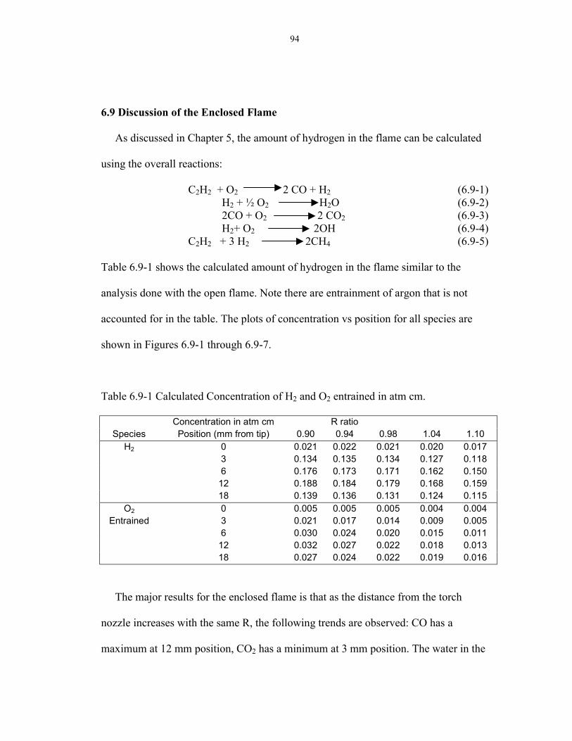
94

6.9 Discussion of the Enclosed Flame

As discussed in Chapter 5, the amount of hydrogen in the flame can be calculated

using the overall reactions:

C2H2 + O2 2 CO + H2 (6.9-1)H2 + ½ O2 H2O (6.9-2)2CO + O2 2 CO2 (6.9-3)H2+ O2 2OH (6.9-4)

C2H2 + 3 H2 2CH4 (6.9-5)

Table 6.9-1 shows the calculated amount of hydrogen in the flame similar to the

analysis done with the open flame. Note there are entrainment of argon that is not

accounted for in the table. The plots of concentration vs position for all species are

shown in Figures 6.9-1 through 6.9-7.

Table 6.9-1 Calculated Concentration of H2 and O2 entrained in atm cm.

Concentration in atm cm R ratioSpecies Position (mm from tip) 0.90 0.94 0.98 1.04 1.10

H2 0 0.021 0.022 0.021 0.020 0.0173 0.134 0.135 0.134 0.127 0.1186 0.176 0.173 0.171 0.162 0.15012 0.188 0.184 0.179 0.168 0.15918 0.139 0.136 0.131 0.124 0.115

O2 0 0.005 0.005 0.005 0.004 0.004Entrained 3 0.021 0.017 0.014 0.009 0.005

6 0.030 0.024 0.020 0.015 0.01112 0.032 0.027 0.022 0.018 0.01318 0.027 0.024 0.022 0.019 0.016

The major results for the enclosed flame is that as the distance from the torch

nozzle increases with the same R, the following trends are observed: CO has a

maximum at 12 mm position, CO2 has a minimum at 3 mm position. The water in the

95

flame increases with increasing distance from the nozzle at low R but maximizes at

12 mm at high R. The acetylene decreases with increasing axial position with

methane appearing only in the 0 mm position with R = 0.90. The OH is not detected

at all. The O2 entrainment and H2 are at maximum at the 12 mm axial position.

With the same position and increasing R, the following trends are observed: CO,

H2, and C2H2 tend to decrease. CO2, O2 entrained, and H2O tend to increase. Table

6.11-1 summarizes these results.

6.10 Oxygen Entrainment in the Enclosed Flame

Theoretically, there should not be any oxygen entrainment in the enclosed flame if

the apparatus is totally leak-proof. However, the apparatus may have a small leakage

from air in the atmosphere. The amount of O2 �entrainment� in the enclosed flame,

however, is only two to three times less than that of the free flame, if the amount of

carbon radicals is neglected. This is because the amount of oxygen fed to the torch is

based on the amount of acetylene back calculated from the observed species (CO2,

and CO). If there are carbon radicals and/or C2 species in the flame, then the actual

amount of acetylene fed to the torch would be higher, thereby increasing the

calculated oxygen feed and decreasing the calculated oxygen entrainment. The

assumption that there are very little carbon radicals and C2 may not be valid.

Therefore, the amount of O2 entraiment here is the maximum amount of entrainment.

The amount of O2 entrainment is lower at the 18 mm position for a reason. The

carbon radicals that are not observable by the FTIR (but could be present) in the

96

regions closer to the torch nozzle are now reacted to form CO and CO2. Since the

calculation for oxygen entrainment is based on the amount of CO and CO2 species

observed, this will decrease the oxygen entrainment. This is because more of the

carbon is now observable, therefore increasing the calculated amount of oxygen fed

to the torch.

6.11 Comparison of the Free and Enclosed Flame

No authors have done work in analyzing the concentration of the species in an

enclosed flame. One of the reasons is that it is very difficult to carry out analytical

techniques in an enclosed atmosphere. Therefore, no comparison to others can be

made.

Soot is observed in the enclosed flame at the 0 mm position. The temperature of

the soot is close to the temperature of the acetylene. In the enclosed flame, there are

no signs of OH in the flame under diamond growing conditions (fuel rich). This is

consistent with the theory that OH is not important for diamond deposition [1] and the

enclosed flame grows diamond films at a higher quality. [2]

The amount of acetylene in the 0 mm position is about the same for open and

enclosed flame. However, methane is observed in the enclosed flame at axial position

close to the nozzle and at low R. Both observations are consistent with the fact that

diamond is grown near the cone.

There is much more CO in the enclosed flame at positions greater than 3 mm from

the nozzle. Since there is no oxygen in the enclosed flame surroundings, the

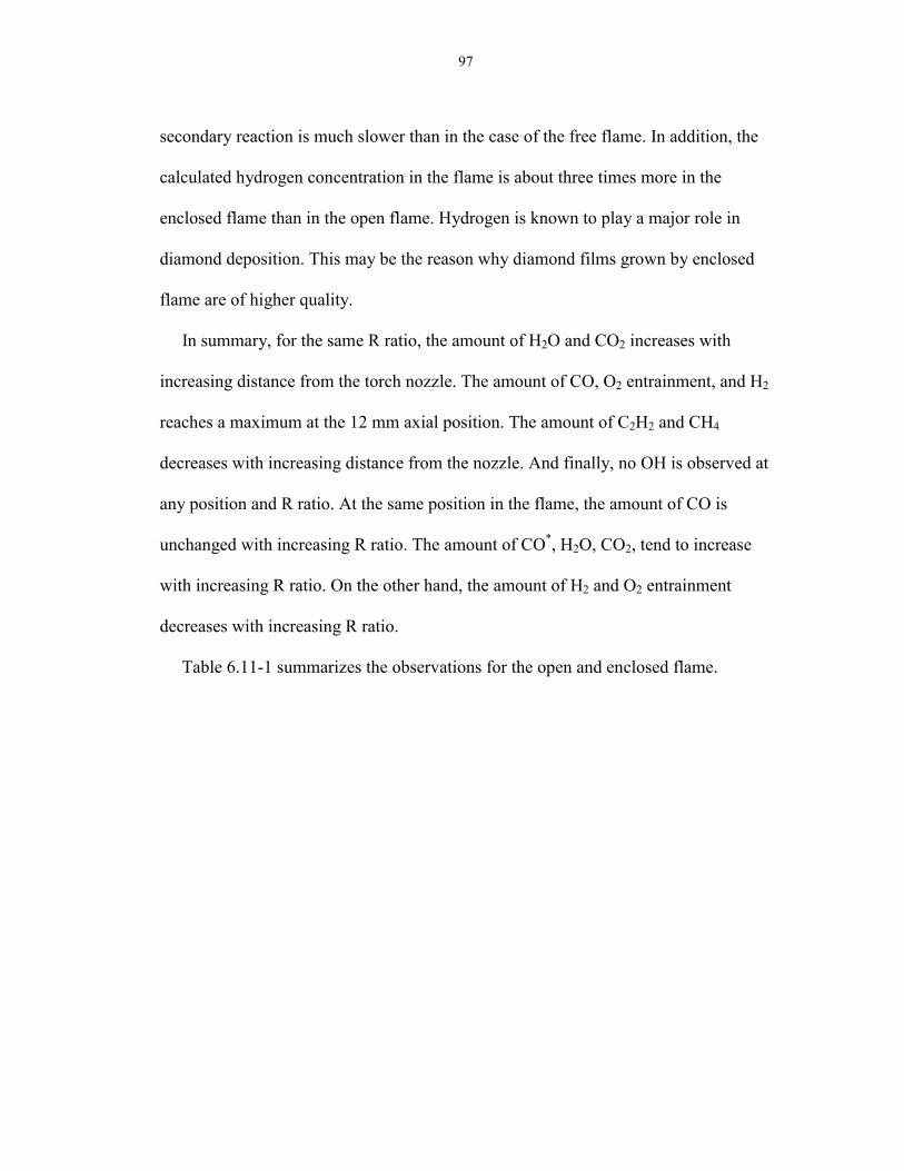
97

secondary reaction is much slower than in the case of the free flame. In addition, the

calculated hydrogen concentration in the flame is about three times more in the

enclosed flame than in the open flame. Hydrogen is known to play a major role in

diamond deposition. This may be the reason why diamond films grown by enclosed

flame are of higher quality.

In summary, for the same R ratio, the amount of H2O and CO2 increases with

increasing distance from the torch nozzle. The amount of CO, O2 entrainment, and H2

reaches a maximum at the 12 mm axial position. The amount of C2H2 and CH4

decreases with increasing distance from the nozzle. And finally, no OH is observed at

any position and R ratio. At the same position in the flame, the amount of CO is

unchanged with increasing R ratio. The amount of CO*, H2O, CO2, tend to increase

with increasing R ratio. On the other hand, the amount of H2 and O2 entrainment

decreases with increasing R ratio.

Table 6.11-1 summarizes the observations for the open and enclosed flame.

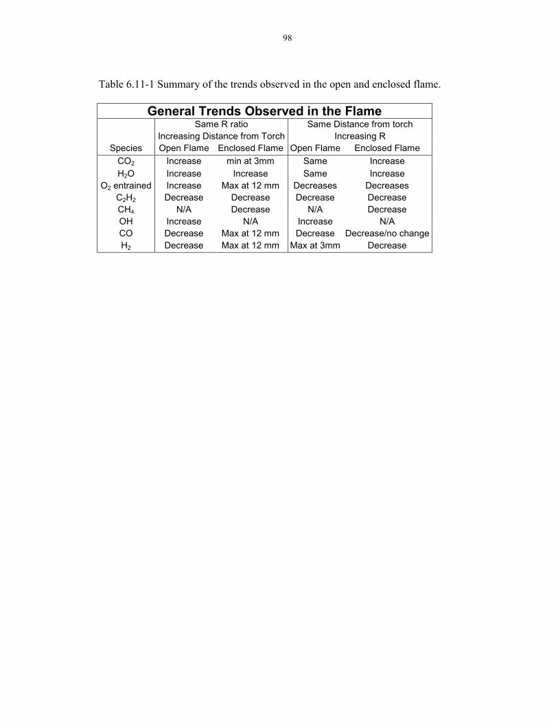
98

Table 6.11-1 Summary of the trends observed in the open and enclosed flame.

General Trends Observed in the FlameSame R ratio Same Distance from torch

Increasing Distance from Torch Increasing RSpecies Open Flame Enclosed Flame Open Flame Enclosed Flame

CO2 Increase min at 3mm Same IncreaseH2O Increase Increase Same Increase

O2 entrained Increase Max at 12 mm Decreases DecreasesC2H2 Decrease Decrease Decrease DecreaseCH4 N/A Decrease N/A DecreaseOH Increase N/A Increase N/ACO Decrease Max at 12 mm Decrease Decrease/no changeH2 Decrease Max at 12 mm Max at 3mm Decrease

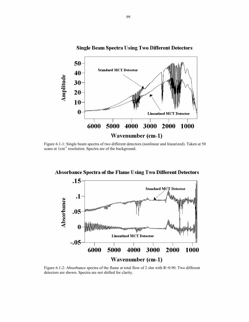
99

Figure 6.1-1: Single beam spectra of two different detectors (nonlinear and linearized). Taken at 50scans at 1cm-1 resolution. Spectra are of the background.

Figure 6.1-2: Absorbance spectra of the flame at total flow of 2 slm with R=0.90. Two differentdetectors are shown. Spectra are not shifted for clarity.

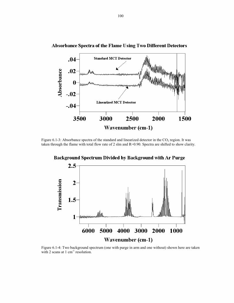
100

Figure 6.1-3: Absorbance spectra of the standard and linearized detector in the CO2 region. It wastaken through the flame with total flow rate of 2 slm and R=0.90. Spectra are shifted to show clarity.

Figure 6.1-4: Two background spectrum (one with purge in arm and one without) shown here are takenwith 2 scans at 1 cm-1 resolution.

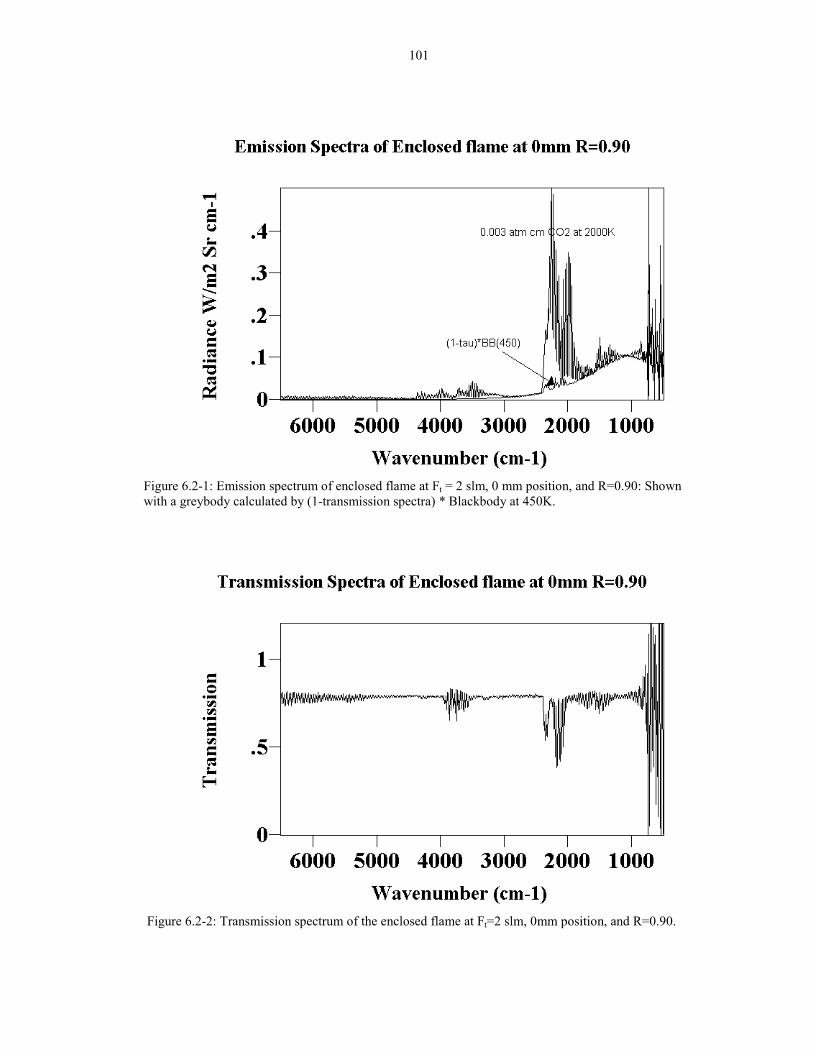
101

Figure 6.2-1: Emission spectrum of enclosed flame at Ft = 2 slm, 0 mm position, and R=0.90: Shownwith a greybody calculated by (1-transmission spectra) * Blackbody at 450K.

Figure 6.2-2: Transmission spectrum of the enclosed flame at Ft=2 slm, 0mm position, and R=0.90.

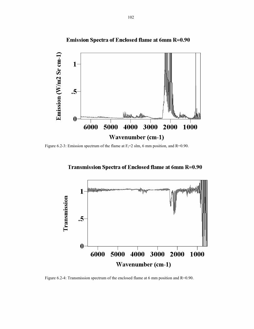
102

Figure 6.2-3: Emission spectrum of the flame at Ft=2 slm, 6 mm position, and R=0.90.

Figure 6.2-4: Transmission spectrum of the enclosed flame at 6 mm position and R=0.90.

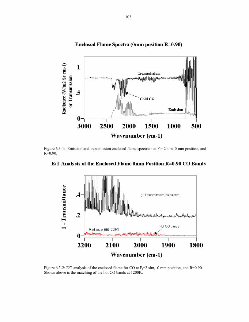
103

Figure 6.3-1: Emission and transmission enclosed flame spectrum at Ft= 2 slm, 0 mm position, andR=0.90.

Figure 6.3-2: E/T analysis of the enclosed flame for CO at Ft=2 slm, 0 mm position, and R=0.90.Shown above is the matching of the hot CO bands at 1200K.

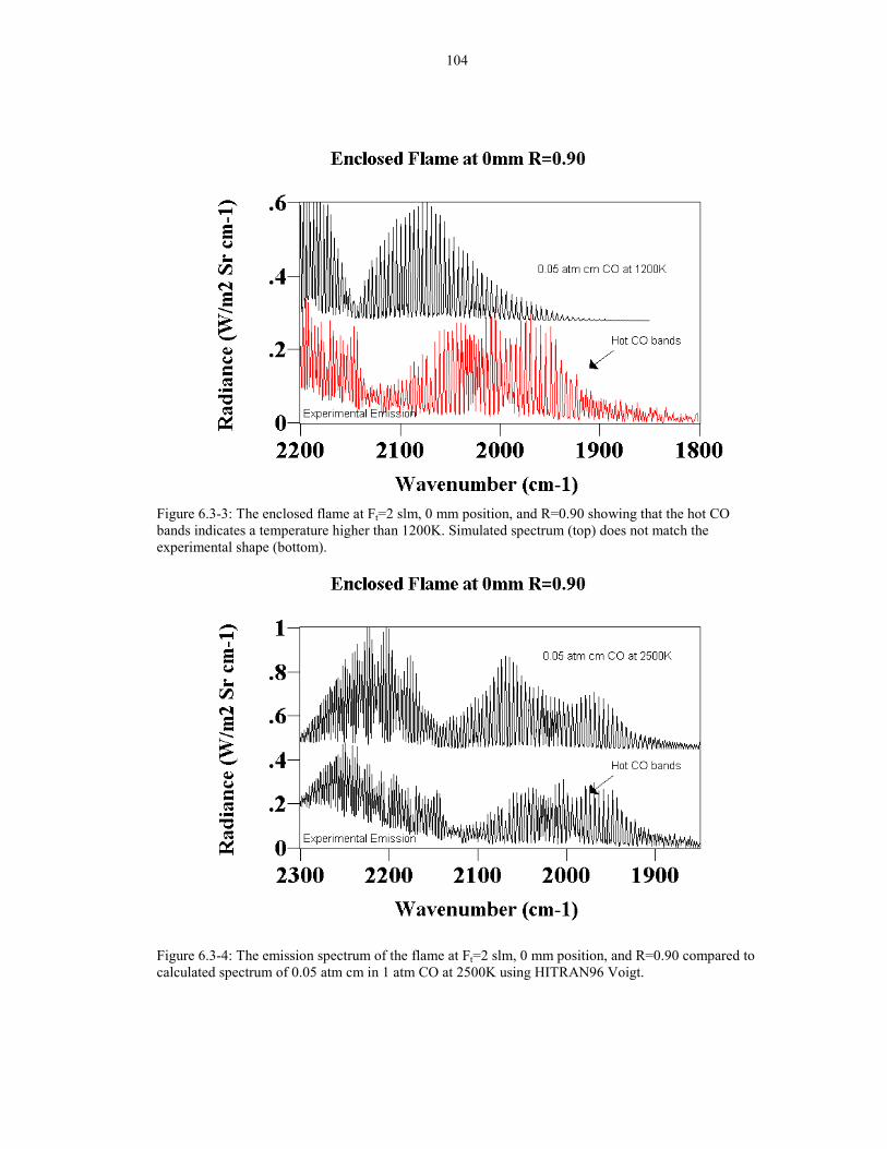
104

Figure 6.3-3: The enclosed flame at Ft=2 slm, 0 mm position, and R=0.90 showing that the hot CObands indicates a temperature higher than 1200K. Simulated spectrum (top) does not match theexperimental shape (bottom).

Figure 6.3-4: The emission spectrum of the flame at Ft=2 slm, 0 mm position, and R=0.90 compared tocalculated spectrum of 0.05 atm cm in 1 atm CO at 2500K using HITRAN96 Voigt.

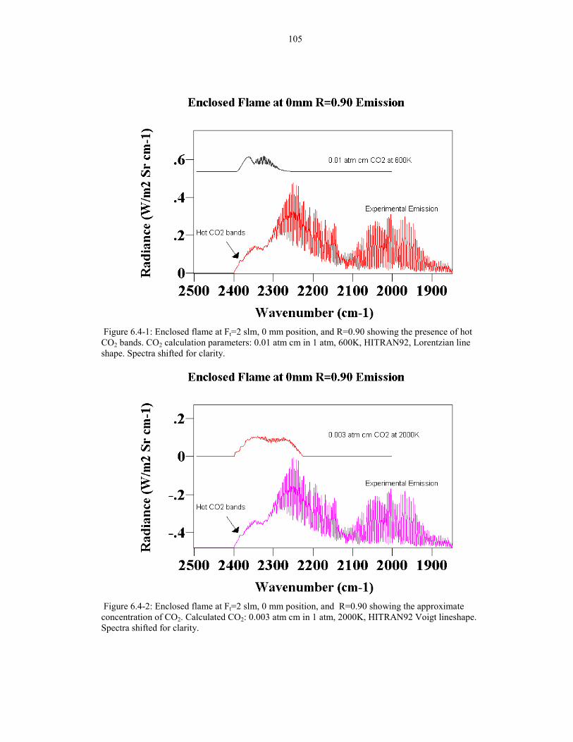
105

Figure 6.4-1: Enclosed flame at Ft=2 slm, 0 mm position, and R=0.90 showing the presence of hotCO2 bands. CO2 calculation parameters: 0.01 atm cm in 1 atm, 600K, HITRAN92, Lorentzian lineshape. Spectra shifted for clarity.

Figure 6.4-2: Enclosed flame at Ft=2 slm, 0 mm position, and R=0.90 showing the approximateconcentration of CO2. Calculated CO2: 0.003 atm cm in 1 atm, 2000K, HITRAN92 Voigt lineshape.Spectra shifted for clarity.

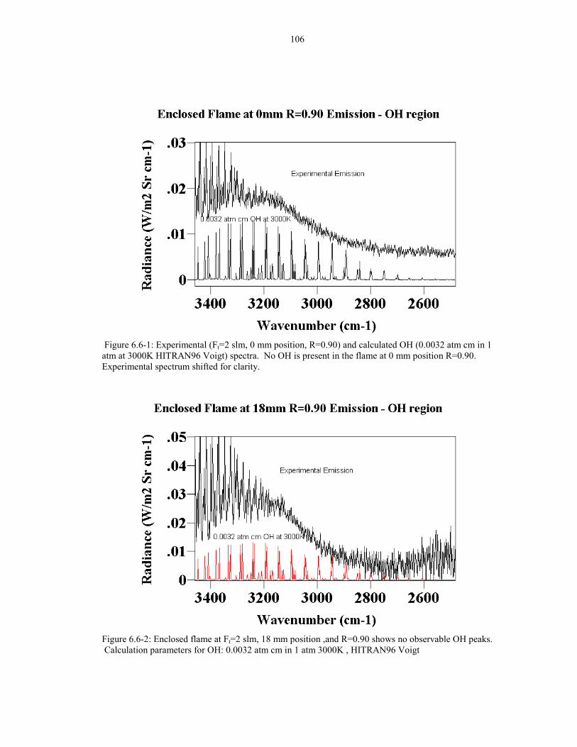
106

Figure 6.6-1: Experimental (Ft=2 slm, 0 mm position, R=0.90) and calculated OH (0.0032 atm cm in 1atm at 3000K HITRAN96 Voigt) spectra. No OH is present in the flame at 0 mm position R=0.90.Experimental spectrum shifted for clarity.

Figure 6.6-2: Enclosed flame at Ft=2 slm, 18 mm position ,and R=0.90 shows no observable OH peaks. Calculation parameters for OH: 0.0032 atm cm in 1 atm 3000K , HITRAN96 Voigt

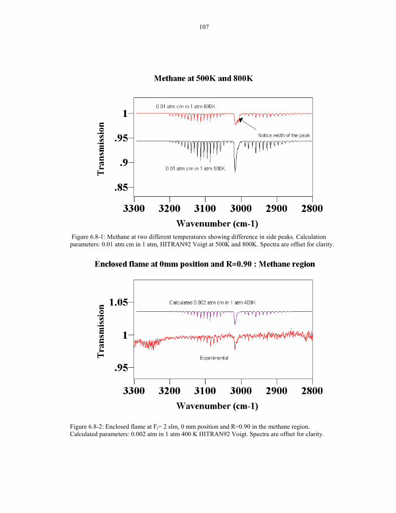
107

Figure 6.8-1: Methane at two different temperatures showing difference in side peaks. Calculationparameters: 0.01 atm cm in 1 atm, HITRAN92 Voigt at 500K and 800K. Spectra are offset for clarity.

Figure 6.8-2: Enclosed flame at Ft= 2 slm, 0 mm position and R=0.90 in the methane region.Calculated parameters: 0.002 atm in 1 atm 400 K HITRAN92 Voigt. Spectra are offset for clarity.

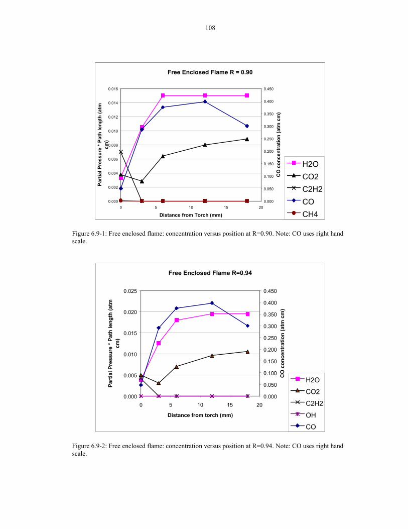
108

Free Enclosed Flame R = 0.90

0.000

0.002

0.004

0.006

0.008

0.010

0.012

0.014

0.016

0 5 10 15 20

Distance from Torch (mm)

Part

ial P

ress

ure

* Pat

h le

ngth

(atm

cm

)

0.000

0.050

0.100

0.150

0.200

0.250

0.300

0.350

0.400

0.450

CO

con

cent

ratio

n (a

tm c

m)

H2OCO2C2H2COCH4

Figure 6.9-1: Free enclosed flame: concentration versus position at R=0.90. Note: CO uses right handscale.

Free Enclosed Flame R=0.94

0.000

0.005

0.010

0.015

0.020

0.025

0 5 10 15 20

Distance from torch (mm)

Part

ial P

ress

ure

* Pat

h le

ngth

(atm

cm

)

0.000

0.050

0.100

0.150

0.200

0.250

0.300

0.350

0.400

0.450C

O c

once

ntra

tion

(atm

cm

)

H2O

CO2

C2H2

OH

CO

Figure 6.9-2: Free enclosed flame: concentration versus position at R=0.94. Note: CO uses right handscale.

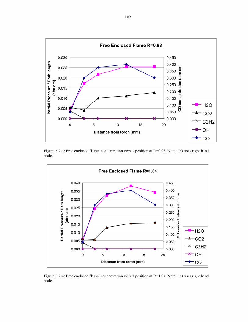
109

Free Enclosed Flame R=0.98

0.000

0.005

0.010

0.015

0.020

0.025

0.030

0 5 10 15 20

Distance from torch (mm)

Part

ial P

ress

ure

* Pat

h le

ngth

(a

tm c

m)

0.000

0.050

0.100

0.150

0.200

0.250

0.300

0.350

0.400

0.450

CO

con

cent

ratio

n (a

tm c

m)

H2O

CO2

C2H2

OH

CO

Figure 6.9-3: Free enclosed flame: concentration versus position at R=0.98. Note: CO uses right handscale.

Free Enclosed Flame R=1.04

0.000

0.005

0.010

0.015

0.020

0.025

0.030

0.035

0.040

0 5 10 15 20

Distance from torch (mm)

Part

ial P

ress

ure

* Pat

h le

ngth

(a

tm c

m)

0.000

0.050

0.100

0.150

0.200

0.250

0.300

0.350

0.400

0.450C

O c

once

ntra

tion

(atm

cm

)

H2O

CO2C2H2OHCO

Figure 6.9-4: Free enclosed flame: concentration versus position at R=1.04. Note: CO uses right handscale.

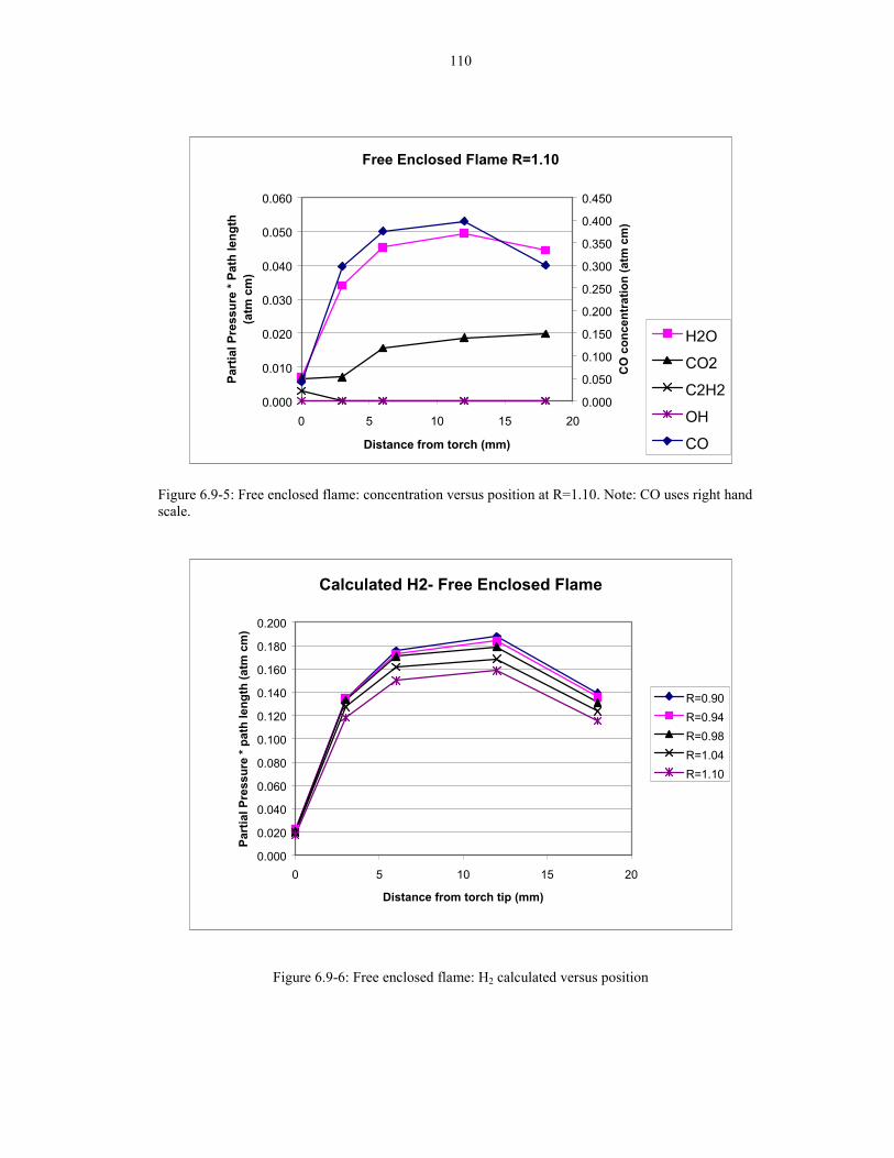
110

Free Enclosed Flame R=1.10

0.000

0.010

0.020

0.030

0.040

0.050

0.060

0 5 10 15 20

Distance from torch (mm)

Part

ial P

ress

ure

* Pat

h le

ngth

(a

tm c

m)

0.000

0.050

0.100

0.150

0.200

0.250

0.300

0.350

0.400

0.450

CO

con

cent

ratio

n (a

tm c

m)

H2O

CO2

C2H2

OH

CO

Figure 6.9-5: Free enclosed flame: concentration versus position at R=1.10. Note: CO uses right handscale.

Calculated H2- Free Enclosed Flame

0.000

0.020

0.040

0.060

0.080

0.100

0.120

0.140

0.160

0.180

0.200

0 5 10 15 20

Distance from torch tip (mm)

Part

ial P

ress

ure

* pat

h le

ngth

(atm

cm

)

R=0.90R=0.94R=0.98R=1.04R=1.10

Figure 6.9-6: Free enclosed flame: H2 calculated versus position

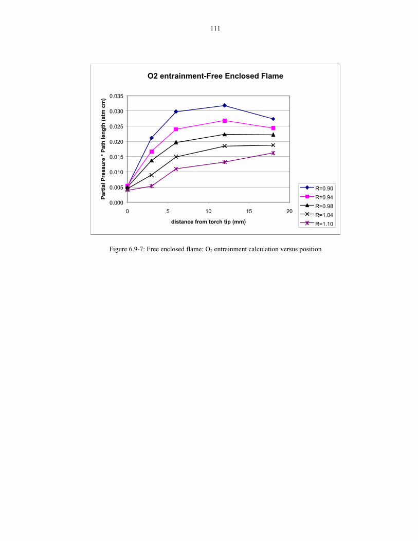
111

O2 entrainment-Free Enclosed Flame

0.000

0.005

0.010

0.015

0.020

0.025

0.030

0.035

0 5 10 15 20

distance from torch tip (mm)

Part

ial P

ress

ure

* Pat

h le

ngth

(atm

cm

)

R=0.90R=0.94R=0.98R=1.04R=1.10

Figure 6.9-7: Free enclosed flame: O2 entrainment calculation versus position

112

7.0 CONCLUSION

Fourier transform infrared spectroscopy has been employed to determine species

concentrations in an oxyacetylene flame. To obtain quantitative measurements of the

oxyacetylene flame using the FTIR, methods to reduce the noise of the flame have

been investigated. One method uses a two detector configuration where one detector

detects the signal plus noise and the other detects just noise. However, the flame does

not emit symmetrically, so this method does not work. A second method uses an

aperture to reduce the amount of noise hitting the detector, but the signal to noise

ratio does not improve using apertures. Another method that does reduce noise is

inverting the torch such that the torch points upward. This method reduces the flame

noise because the flow is now in the direction of buoyant forces. Finally, the use of an

infrared filter to block out the CO2 and CO emission was also efficient in reducing the

noise in the low wavenumber regions.

Once the noise of the flame is minimized, emission/transmission FTIR analysis

was used in conjunction with the HITRAN database to obtain quantitative

information on various species in the flame. The average temperature of the species

along with the maximum temperature have been determined. Quantitative analyses of

the free oxyacetylene flame are carried out in an open and enclosed environment.

Concentrations of species CO, CO2, H2O, OH, CH4, and C2H2 are found, and the

amounts of H2 and O2 entrainment to the flame are calculated. We find that the

enclosed flame contains much more CO and hydrogen than the open flame. This

could be the reason why diamond films grown in the enclosed flame are higher in

113

quality. In addition to the increase amount of hydrogen and CO, the OH disappears

and the hydrogen concentration reachs a maximum at 3 mm from the torch nozzle

(where diamond deposition occurs). In the case of the open flame, we calculate that

the oxygen entrainment increases with increasing distance from the flame. However,

for the enclosed flame, the oxygen entrainment somewhat decreases with increasing

distance. From the way the oxygen entrainment is calculated, this indicates that there

were substantially higher amounts of carbon radical (or atoms) in the enclosed flame,

which cannot be detected by the FTIR. These carbon radicals can play a major role in

diamond deposition.

The detection limits for acetylene, methane, and OH radicals have been

determined. We find that acetylene is observed only at the 0 mm axial position, and

methane is seen only at the 0 mm axial position (R = 0.90) in the enclosed flame.

In addition to gases, particles of soot are also observed in the enclosed flame at the

0 mm axial position. Since this is a carbon rich region, it is not surprising that soot is

formed here.

The HITRAN database was a very useful tool. Using HITRAN, we are able to

calculate quantitatively spectra close to that of the experimental data, making

quantitative analysis possible. However, there are some shortcomings for the

software. It was found that HITEMP, HITRAN do not correctly calculate the CO2

bands at high temperature, and the acetylene band at 730 cm-1 is overcalculated.

Furthermore, the HITEMP CO database does not work well with HITRAN96 because

114

the HITEMP database contains numbers that are too small and causes an overflow in

the program.

Despite all the quantitative results, there are some limitations to using the FTIR.

The exact path length is unknown, making the calculation of the species partial

pressures impossible. In addition, since this is a line of sight measurement, the

concentrations reported here are average and not point concentrations. Furthermore,

with the FTIR method, it is not possible to analyze for carbon radicals in the flame.

There may be substantial amounts of carbon radicals in the enclosed flame, as seen in

the oxygen entrainment calculations.

115

8.0 FUTURE WORK

In order to achieve a better understanding of how the flame varies with a substrate

in place depositing diamond, additional experiments are needed. First, the FTIR

should be used to make measurements of the flame with the substrate in place while

depositing diamond films. The gas phase composition of the flame may change when

diamond films are depositing due to further reactions on the surface of the substrate.

The films should then be analyzed for its growth rate and quality in order to correlate

diamond growth to species concentration.

Secondly, the FTIR should be coupled with the cascade arc so that a higher

intensity IR source can be used. This higher intensity source will enable an aperture

to be placed in between the substrate and the IR source to gain spatial resolution. The

3 mm spot size used in these experiments is too large since the deposition distance is

less than 1 mm from the inner cone. Therefore, it is necessary to obtain spatial

resolution of less than 1 mm. If the cascade arc is used, it will be possible to probe the

boundary layer.

Another idea for future work is to use a faster FTIR so that the Fourier frequencies

are greater than the flickering frequencies. This will aid in reducing the noise in the

spectrum. With the use of the cascade arc, apertures, and faster FTIR, the signal to

noise ratio and spatial resolution will substantially increase.

Lastly, tomography should be considered for spatial resolution. Also, some of the

problems encountered with CO in the enclosed flame apparatus may be minimized

because the location of the cold CO will be more apparent.

116

Chapter One References

[1] J. C. Angus and C. C. Hayman, "Low-pressure, metastable growth of diamondand diamondlike phases," Science 241, 913 (1988).

[2] D. S. Knight and W. B. White, "Characterization of diamond films by Ramanspectroscopy," J. Mater. Res. 4, 385 (1989).

[3] D. B. Oakes and J. E. Butler, "Diamond synthesis in oxygen-acetylene flames:Inhomogeneities and the effects of hydrogen addition," J. Appl. Phys.69, 2602 (1991).

[4] L. M. Hanssen, K. A. Snail, W. A. Carrington, J. E. Butler, S. Kellogg, and D.B. Oakes, "Diamond and non-diamond carbon synthesis in an oxygen-acetylene flame," Thin Solid Films 196, 271 (1991).

[5] J. C. Angus, Y. Wang, and M. Sunkara, "Metastable growth of diamond anddiamondlike phases," Ann. Rev. Mat. Sci. 21, 221 (1991).

[6] J. C. Angus, M. Sunkara, S. R. Sahaida, and J. T. Glass, "Twinning and facetingin early stages of diamond growth by chemical vapor deposition," J.Mater. Res. 7, 3001 (1992).

[7] J.-S. Lee and K.-S. Liu, "Deposition of diamond films on SiO2 surfaces using ahigh power microwave enhanced chemical vapor deposition process," J.Appl. Phys. 81, 486 (1996).

[8] R. Locher, C. Wild, N. Herres, D. Behr, and P. Koidl, "Nitrogen Stabilized(100) Texture In Chemical-Vapor-Deposited Diamond Films," Appl.Phys. Lett. 65(1), 34 (1994).

[9] M. Kamo, Y. Sato, S. Matsumoto, and S. Setaka, "," J. Cryst. Growth 62, 642(1983).

[10] Y. Matsui, H. Yabe, T. Sugimoto, and Y. Hirose, "The structure of acetyleneflames for diamond synthesis," Diam. Related Mater. 1, 19 (1991).

[11] Y. Hirose and N. Kondo, Program and Book of Abstracts, Japan AppliedPhysics, 1988 Spring Meeting (Japanese Physical Society, Tokyo,1988), p. 434.

[12] L. A. Zeatoun and P. W. Morrison Jr., "Optimizing diamond growth for anatmospheric oxyacetylene torch," J. Mater. Res. 12, 1237 (1997).

117

[13] K. Doverspike, J. E. Butler, and J. A. Freitas Jr., "Deposition of flame growndiamond films in a controlled atmosphere" in Materials ResearchSociety Symposium Proceedings: Wide Band Gap Semiconductors,edited by T. D. Moustakas, J. I. Pankove, and Y. Hamakawa (MaterialsResearch Society, Pittsburgh, PA, 1992), Vol. 242, p. 37.

[14] J. J. Schermer, J. E. M. Hogenkamp, G. C. J. Otter, G. Janssen, W. J. P. vanEnckevort, and L. J. Giling, "Controlled deposition of diamond from anacetylene-oxygen combustion flame," Diam. Related Mater. 2, 1149(1993).

[15] Y. Hirose and S. Amanuma, "The synthesis of high quality diamond incombustion flames," J. Appl. Phys. 68, 6401 (1990).

[16] P. W. Morrison Jr., A. Somashekhar, J. T. Glass, and J. T. Prater, "Growth ofdiamond films using an enclosed combustion flame," J. Appl. Phys. 78,4144 (1995).

[17] P. W. Morrison Jr., J. E. Cosgrove, J. R. Markham, and P. R. Solomon, "In-SituIR Spectroscopy of an Oxygen-Acetylene Flame During Diamond FilmGrowth," Carbon 28, 767 (1990).

[18] P. W. Morrison Jr., J. E. Cosgrove, J. R. Markham, and P. R. Solomon,"Tomographic reconstruction of FT-IR measurements of an oxygen-acetylene flame during diamond film growth" in MRS InternationalConference Proceedings Series: New Diamond Science and Technology(Proceedings of the Second International Conference on New DiamondScience and Technology, edited by R. Messier, J. T. Glass, J. E. Butler,and R. Roy (Materials Research Society, Pittsburgh, PA, 1991), p. 219.

Chapter Two References

[1] P. W. Morrison Jr. and J. T. Glass, "Flame characteristics for combustiongrowth of diamond" in EMIS Datareview Series: Properties andGrowth of Diamond, edited by G. Davies (Institution of ElectricalEngineers, London, UK, 1994), Vol. 9, p. 368.

[2] Y. Hirose and S. Amanuma, "The synthesis of high quality diamond incombustion flames," J. Appl. Phys. 68, 6401 (1990).

118

[3] R.-B. Wang, M. Sommer, and F. W. Smith, "Deposition of diamond films viathe oxyacetylene torch: experimental results and thermodynamicpredictions," J. Cryst. Growth 119, 271 (1992).

[4] L. M. Hanssen, K. A. Snail, W. A. Carrington, J. E. Butler, S. Kellogg, and D.B. Oakes, "Diamond and non-diamond carbon synthesis in an oxygen-acetylene flame," Thin Solid Films 196, 271 (1991).

[5] J. J. Schermer, J. E. M. Hogenkamp, G. C. J. Otter, G. Janssen, W. J. P. vanEnckevort, and L. J. Giling, "Controlled deposition of diamond from anacetylene-oxygen combustion flame," Diam. Related Mater. 2, 1149(1993).

[6] K. Bang, A. J. Ghajar, and R. Komanduri, "The effect of substrate surfacetemperature on the morphology and quality of diamond films producedby the oxyacetylene combustion flame," Thin Solid Films 238, 172(1994).

[7] L. A. Zeatoun and P. W. Morrison Jr., "Optimizing diamond growth for anatmospheric oxyacetylene torch," J. Mater. Res. 12, 1237 (1997).

[8] S. Marinkovic and S. Zec, "Formation of large diamond crystals inoxyacetylene flame chemical vapour deposition," J. Mat. Sci. 31, 5999(1996).

[9] W. Zhu, B. H. Tan, J. Ahn, and H. S. Tan, "Studies of diamond films/crystalssynthesized by oxyacetylene combustion flame technique," J. Mat. Sci.30, 2130 (1995).

[10] D. W. Zhang, Z. J. Liu, Y. Z. Wan, and J. T. Wang, "Phase Diagram fordiamond growth in atmospheric oxyacetylene flames," J. Appl. Phys.66, 49 (1998).

[11] K. A. Snail, R. G. Vardiman, J. P. Estrera, J. W. Glesener, C. Merzbacher, C. J.Craigie, C. M. Marks, R. Glosser, and J. A. Freitas Jr., "Diamondgrowth in turbulent oxygen-acetylene flames," J. Appl. Phys. 74, 7561(1993).

[12] R. Phillips, J. Wei, and Y. Tzeng, "High quality flame-deposited diamond filmsfor IR optical windows," Thin Solid Films 212, 30 (1992).

[13] M. Murakawa, S. Takeuchi, and Y. Hirose, "An experiment in large areadiamond coating using a combustion flame torch in its traversingmode," Surf. Coat. Technol. 43-44, 22 (1990).

119

[14] M. Murakawa and S. Takeuchi, "Diamond coating using multiple flame torchesin an atmospheric chamber," Surf. Coat. Technol. 54/55, 403 (1992).

[15] K. Doverspike, J. E. Butler, and J. A. Freitas Jr., "Deposition of flame growndiamond films in a controlled atmosphere" in Materials ResearchSociety Symposium Proceedings: Wide Band Gap Semiconductors,edited by T. D. Moustakas, J. I. Pankove, and Y. Hamakawa (MaterialsResearch Society, Pittsburgh, PA, 1992), Vol. 242, p. 37.

[16] P. W. Morrison Jr., A. Somashekhar, J. T. Glass, and J. T. Prater, "Growth ofdiamond films using an enclosed combustion flame," J. Appl. Phys. 78,4144 (1995).

[17] F. R. Sivazlian, J. A. von Windheim, and J. T. Glass, "Diamond growth in anoxy-acetylene flame by an alternating gas ratio technique" in MaterialsResearch Society Symposium Proceedings: Novel Forms of Carbon,edited by C. L. Renschler, J. J. Pouch, and D. M. Cox (MaterialsResearch Society, Pittsburgh, PA, 1992), Vol. 270, p. 329.

[18] J. A. von Windheim, F. Sivazlian, M. T. McClure, and J. T. Glass, "Nucleationand growth of diamond using a computer controlled oxy-acetylenetorch," Diam. Related Mater. 2, 438 (1993).

[19] Y. Matsui, H. Yabe, T. Sugimoto, and Y. Hirose, "The structure of acetyleneflames for diamond synthesis," Diam. Related Mater. 1, 19 (1991).

[20] R. S. Yalamanchi and K. S. Harshavardham, "Diamond growth in combustionflames," J. Appl. Phys. 68(11), 5941 (1990).

[21] Y. Matsui, A. Yuuki, M. Sahara, and Y. Hirose, "Flame structure and diamondgrowth mechanism of acetylene torch," Jpn. J. Appl. Phys. 28, 1718(1989).

[22] R. J. H. Klein-Douwel, J. J. L. Spaanjaars, and J. J. ter Meulen, "Two-dimensional distribution of C2, CH, and OH in a diamond depositingoxyacetylene flame measured by laser induced fluorescence," J. Appl.Phys. 78 (3), 2086 (1995).

[23] M. A. Cappelli and P. H. Paul, "An investigation of diamond film deposition ina premixed oxyacetylene flame," J. Appl. Phys. 67 (5), 2596 (1989).

120

[24] M. D. Welter and K. L. Menningen, "Radical Density measurements in anoxyacetylene torch diamond growth flame," J. Appl. Phys. 82(4), 1900(1997).

[25] C. M. Marks, H. R. Burris, J. L. Grun, and K. A. Snail, "Studies of turbulentoxyacetylene flames used for diamond growth," J. Appl. Phys. 73, 755(1993).

[26] C. A. Wolden, R. F. Davis, and Z. Sitar, "In situ mass spectrometry duringdiamond chemical vapor deposition using a low pressure flat flame," J.Mater. Res. 12(10), 2733 (1997).

[27] P. W. Morrison Jr. and J. R. Haigis, "In situ infrared measurements of film andgas properties during the plasma deposition of amorphous hydrogenatedsilicon," J. Vac. Sci. Technol. A 11, 490 (1993).

[28] P. W. Morrison Jr., R. Raghavan, A. J. Timpone, C. P. Artelt, and S. E.Pratsinis, "in situ Fourier transform infrared characterization ofelectrically assisted flame synthesis of TiO2 particles," Chem. Mat. 9,2702 (1997).

[29] P. W. Morrison Jr., J. E. Cosgrove, J. R. Markham, and P. R. Solomon, "In-SituIR Spectroscopy of an Oxygen-Acetylene Flame During Diamond FilmGrowth," Carbon 28, 767 (1990).

[30] P. W. Morrison Jr., J. E. Cosgrove, J. R. Markham, and P. R. Solomon,"Tomographic reconstruction of FT-IR measurements of an oxygen-acetylene flame during diamond film growth" in MRS InternationalConference Proceedings Series: New Diamond Science and Technology(Proceedings of the Second International Conference on New DiamondScience and Technology, edited by R. Messier, J. T. Glass, J. E. Butler,and R. Roy (Materials Research Society, Pittsburgh, PA, 1991), p. 219.

[31] P. W. Morrison Jr., and O. Taweechokesupsin, Calculation of gas phase spectrafor quantitative Fourier transform infrared spectroscopy of chemicalvapor deposition, {iJ. Electrochem. Soc.}, {b145}, 3212 (1998).

Chapter Three References

[1] L. A. Zeatoun and P. W. Morrison Jr., "Optimizing diamond growth for anatmospheric oxyacetylene torch," J. Mater. Res. 12, 1237 (1997).

121

[2] J. Wang, T. Wang, Z. Zhen, Y. Luo, M. R. Clench, and D. J. Mowthorpe, "Theinfluence of the temperature of blackbody for calibrating FTIR systemon the instrument response function," SPECTROSC. LETT. 30, 783(1997).

[3] P. W. Morrison Jr. and J. R. Haigis, "In situ infrared measurements of film andgas properties during the plasma deposition of amorphous hydrogenatedsilicon," J. Vac. Sci. Technol. A 11, 490 (1993).

Chapter Four References

[1] S. Elfeky, A. Penninger, L. Karpati, and A. Bereczky, "Noise emission fromopen turbulent premixed flame," Periodica Polytechnica, MechanicalEngineering 40 (2), 85 (1995).

[2] L. A. Zeatoun and P. W. Morrison Jr., "Optimizing diamond growth for anatmospheric oxyacetylene torch," J. Mater. Res. 12, 1237 (1997).

Chapter Five References

[1] D. Scutaru, L. Rosenmann, and J. Taine, "Approximate Intensities of CO2 HotBands at 2.7, 4.3, and 12 micron for High Temperature and MediumResolution Applications," J. Quant. Spectrosc. Radiat. Transfer 52, 765(1994).

[2] P. W. Morrison Jr., J. E. Cosgrove, J. R. Markham, and P. R. Solomon,"Tomographic reconstruction of FT-IR measurements of an oxygen-acetylene flame during diamond film growth" in MRS InternationalConference Proceedings Series: New Diamond Science and Technology(Proceedings of the Second International Conference on New DiamondScience and Technology, edited by R. Messier, J. T. Glass, J. E. Butler,and R. Roy (Materials Research Society, Pittsburgh, PA, 1991), p. 219.

[3] P. W. Morrison Jr., J. E. Cosgrove, J. R. Markham, and P. R. Solomon, "In-SituIR Spectroscopy of an Oxygen-Acetylene Flame During Diamond FilmGrowth," Carbon 28, 767 (1990).

122

[4] G. Zhimeng, Y. Sheng, and L. Heyi, "The roles of hydrogen in deposition ofdiamond film using hydrogen-oxyacetylene combustion flame," J. Mat.Sci. Lett. 14, 244 (1995).

[5] Y. Matsui, H. Yabe, T. Sugimoto, and Y. Hirose, "The structure of acetyleneflames for diamond synthesis," Diam. Related Mater. 1, 19 (1991).

[6] P. F. Jessen and A. G. Gaydon, "Estimation of carbon radical concentrations infuel rich acetylene-oxygen flames by absorption spectroscopy" in xxxSymposium (International) on Combustion (Combustion Institute,Pittsburgh, PA, 1968), p. 481.

[7] R. S. Yalamanchi and K. S. Harshavardham, "Diamond growth in combustionflames," J. Appl. Phys. 68(11), 5941 (1990).

[8] Y. Matsui, A. Yuuki, M. Sahara, and Y. Hirose, "Flame structure and diamondgrowth mechanism of acetylene torch," Jpn. J. Appl. Phys. 28, 1718(1989).

[9] R. J. H. Klein-Douwel, J. J. L. Spaanjaars, and J. J. ter Meulen, "Two-dimensional distribution of C2, CH, and OH in a diamond depositingoxyacetylene flame measured by laser induced fluorescence," J. Appl.Phys. 78 (3), 2086 (1995).

[10] M. D. Welter and K. L. Menningen, "Radical Density measurements in anoxyacetylene torch diamond growth flame," J. Appl. Phys. 82(4), 1900(1997).

Chapter Six Reference

[1] R. J. H. Klein-Douwel, J. J. L. Spaanjaars, and J. J. ter Meulen, "Two-dimensional distribution of C2, CH, and OH in a diamond depositingoxyacetylene flame measured by laser induced fluorescence," J. Appl.Phys. 78 (3), 2086 (1995).

[2] P. W. Morrison Jr., A. Somashekhar, J. T. Glass, and J. T. Prater, "Growth ofdiamond films using an enclosed combustion flame," J. Appl. Phys. 78,4144 (1995).

123

Appendix I Conv65K.ab Basic Program

' This program converts a high resolution, simulated transmission' spectrum into a simulated FTIR spectrum at a lower resolution.' The input spectrum is calculated using the HITRAN-PC programcalled' trans.exe at a high resolution (0.1 to 0.01 cm-1 depending onthe' pressure). CONV65K.AB performs an inverse FFT to generate an' equivalent i-gram for the transmission spectrum and thentruncates' the i-gram to reduce the resolution and performs a triangular' apodization on the truncated i-gram. CONV65K.AB thenperforms a' FFT to convert the apodized i-gram to the simulated FTIRspectrum.' Copyright 1995,1996 Philip W. Morrison, Jr.' Case Western Reserve Univ.

freeif getright() < getleft() then xflip ' makes sure lo --> hi

' check number of pointspts = npts #s ' pts = npts of HITRANPC filemm=log(pts)/log(2)xx = mm - int(mm)if xx<>0 then dialogbeg "# of points not = power of 2" :dialogend : stop

' check for correct resolutionfi = getffp() : la = getflp()resinit = abs(la-fi)/(pts - 1) 'resolution of HITRANPC file

if abs(resinit* 32/0.4821686 - 1) <= 1e-6 then goto 100if abs(resinit* 64/0.4821686 - 1) <= 1e-6 then goto 100if abs(resinit*128/0.4821686 - 1) <= 1e-6 then goto 100if abs(resinit*256/0.4821686 - 1) <= 1e-6 then goto 100dialogbeg "Check resolution on HITRANPC spectrum"print "Spectrum resolution is "; resinit; " cm-1"print "Must be 0.0150677, 0.007534 cm-1, or 0.003767 cm-1"print "Probably wrong endpoint values"print " "dialogendstop

100 input "Enter desired cm-1 resolution (1, 2, 4, or 8): "resfinal

if resfinal = 1 then resratio = 1.32/.9643519 : reseff = 1.32' 0.9643519 = nominal resolution of 1 cm-1 MB157' 1.32 = effective resolution of 1 cm-1 MB157, MCT

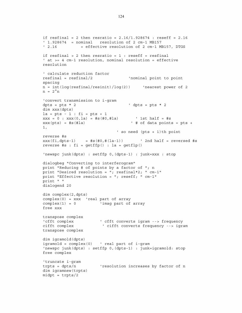
124

if resfinal = 2 then resratio = 2.16/1.928674 : reseff = 2.16' 1.928674 = nominal resolution of 2 cm-1 MB157' 2.16 = effective resolution of 2 cm-1 MB157, DTGS

if resfinal > 2 then resratio = 1 : reseff = resfinal' at >= 4 cm-1 resolution, nominal resolution = effectiveresolution

' calculate reduction factorresfinal = resfinal/2 'nominal point to pointspacingn = int(log(resfinal/resinit)/log(2)) 'nearest power of 2n = 2^n

'convert transmission to i-gramdpts = pts * 2 ' dpts = pts * 2dim xxx(dpts)la = pts - 1 : fi = pts + 1xxx = 0 : xxx(0,la) = #s(#0,#la) ' 1st half = #sxxx(pts) = #s(#la) ' # of data points = pts +1,

' so need (pts + 1)th pointreverse #sxxx(fi,dpts-1) = #s(#0,#(la-1)) ' 2nd half = reversed #sreverse #s : fi = getffp() : la = getflp()

'newspc junk(dpts) : setffp 0,(dpts-1) : junk=xxx : stop

dialogbeg "Converting to interferogram"print "Reducing # of points by a factor of "; nprint "Desired resolution = "; resfinal*2; " cm-1"print "Effective resolution = "; reseff; " cm-1"print " "dialogend 20

dim complex(2,dpts)complex(0) = xxx 'real part of arraycomplex(1) = 0 'imag part of arrayfree xxx

transpose complex'cfft complex ' cfft converts igram --> frequencycifft complex ' cifft converts frequency --> igramtranspose complex

dim igramold(dpts)igramold = complex(0) ' real part of i-gram'newspc junk(dpts) : setffp 0,(dpts-1) : junk=igramold: stopfree complex

'truncate i-gramtrpts = dpts/n 'resolution increases by factor of ndim igramnew(trpts)midpt = trpts/2

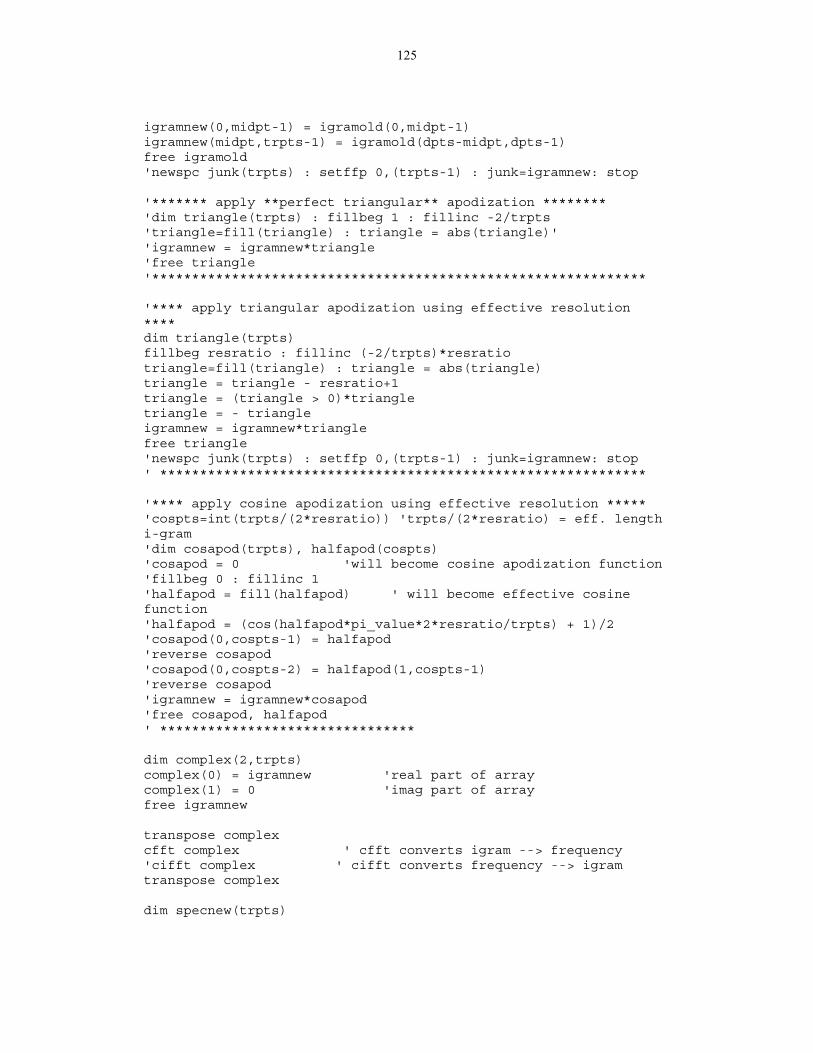
125

igramnew(0,midpt-1) = igramold(0,midpt-1)igramnew(midpt,trpts-1) = igramold(dpts-midpt,dpts-1)free igramold'newspc junk(trpts) : setffp 0,(trpts-1) : junk=igramnew: stop

'******* apply **perfect triangular** apodization ********'dim triangle(trpts) : fillbeg 1 : fillinc -2/trpts'triangle=fill(triangle) : triangle = abs(triangle)''igramnew = igramnew*triangle'free triangle'**************************************************************

'**** apply triangular apodization using effective resolution****dim triangle(trpts)fillbeg resratio : fillinc (-2/trpts)*resratiotriangle=fill(triangle) : triangle = abs(triangle)triangle = triangle - resratio+1triangle = (triangle > 0)*triangletriangle = - triangleigramnew = igramnew*trianglefree triangle'newspc junk(trpts) : setffp 0,(trpts-1) : junk=igramnew: stop' *************************************************************

'**** apply cosine apodization using effective resolution *****'cospts=int(trpts/(2*resratio)) 'trpts/(2*resratio) = eff. lengthi-gram'dim cosapod(trpts), halfapod(cospts)'cosapod = 0 'will become cosine apodization function'fillbeg 0 : fillinc 1'halfapod = fill(halfapod) ' will become effective cosinefunction'halfapod = (cos(halfapod*pi_value*2*resratio/trpts) + 1)/2'cosapod(0,cospts-1) = halfapod'reverse cosapod'cosapod(0,cospts-2) = halfapod(1,cospts-1)'reverse cosapod'igramnew = igramnew*cosapod'free cosapod, halfapod' ********************************

dim complex(2,trpts)complex(0) = igramnew 'real part of arraycomplex(1) = 0 'imag part of arrayfree igramnew

transpose complexcfft complex ' cfft converts igram --> frequency'cifft complex ' cifft converts frequency --> igramtranspose complex

dim specnew(trpts)

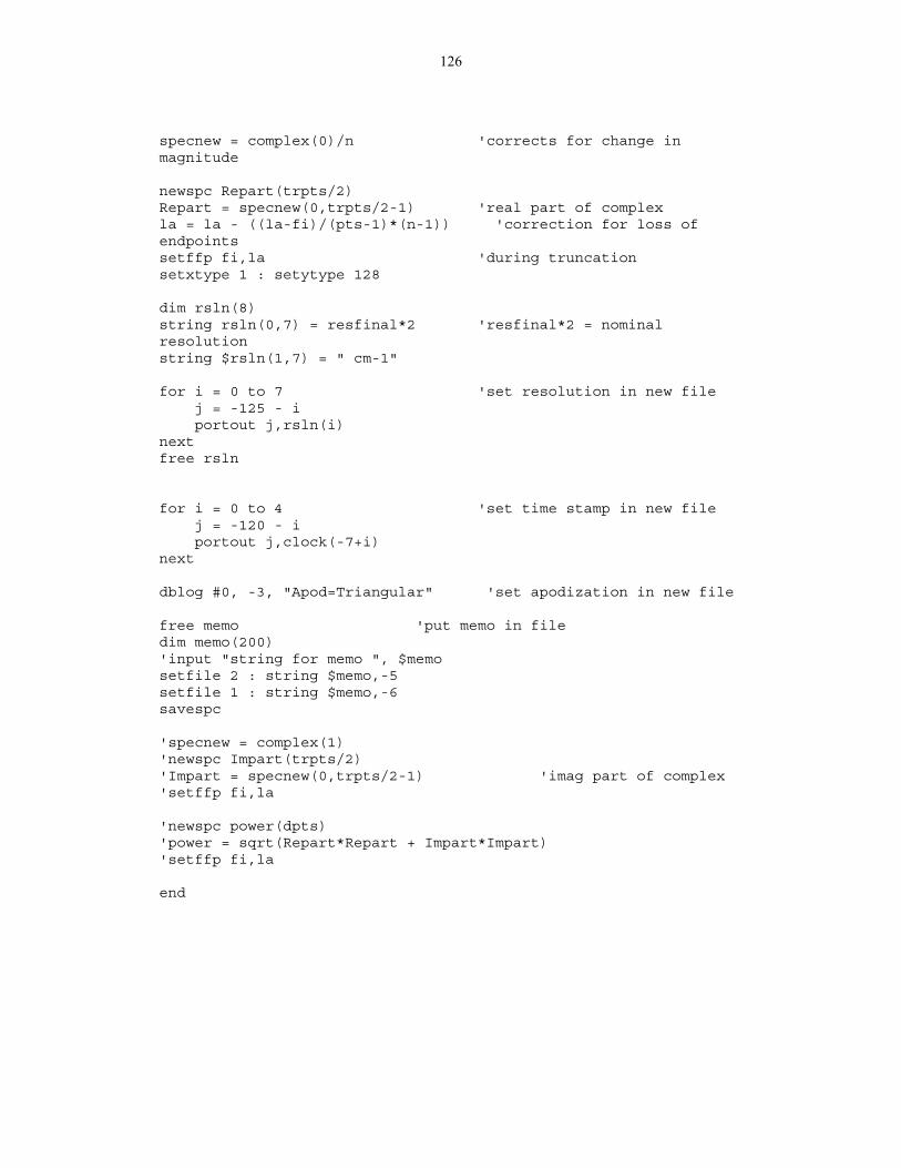
126

specnew = complex(0)/n 'corrects for change inmagnitude

newspc Repart(trpts/2)Repart = specnew(0,trpts/2-1) 'real part of complexla = la - ((la-fi)/(pts-1)*(n-1)) 'correction for loss ofendpointssetffp fi,la 'during truncationsetxtype 1 : setytype 128

dim rsln(8)string rsln(0,7) = resfinal*2 'resfinal*2 = nominalresolutionstring $rsln(1,7) = " cm-1"

for i = 0 to 7 'set resolution in new file j = -125 - i portout j,rsln(i)nextfree rsln

for i = 0 to 4 'set time stamp in new file j = -120 - i portout j,clock(-7+i)next

dblog #0, -3, "Apod=Triangular" 'set apodization in new file

free memo 'put memo in filedim memo(200)'input "string for memo ", $memosetfile 2 : string $memo,-5setfile 1 : string $memo,-6savespc

'specnew = complex(1)'newspc Impart(trpts/2)'Impart = specnew(0,trpts/2-1) 'imag part of complex'setffp fi,la

'newspc power(dpts)'power = sqrt(Repart*Repart + Impart*Impart)'setffp fi,la

end