Diagrams Representing Relationships between …web2.utc.edu/~pbv184/PSY595/L8 - EFA, CFA, and SEM.doc · Web viewREGRESSION /DESCRIPTIVES MEAN STDDEV CORR SIG N /MISSING LISTWISE

EFA, CFA, and SEM(You should have read the EFA chapter in T&F, the Structural Equation Modeling chapter, and be reading the Byrne text.)Observed Variable

A variable whose values are observable.

Examples: IQ Test scores (Scores are directly observable), GREV, GREQ, GREA, UGPA, Minnesota Job Satisfaction Scale, Affective Commitment Scale, Gender, Questionnaire items.

Latent Variable

A variable, i.e., characteristic, presumed to exist, but whose values are NOT observable. A Factor in Factor Analysis literature. A characteristic of people that is not directly observable.

Intelligence, Depression, Job Satisfaction, Affective Commitment, Tendency to display affective state

No direct observation of values of latent variables is possible. Brain states? Brain chemistry?

Indicator

An observed variable whose values are assumed to be related to the values of a latent variable.

Reflective Indicator

An observed variable whose values are partially determined by, i.e., are influenced by or reflect, the values of a latent variable. For example, responses to Conscientiousness items are assumed to reflect a person’s Conscientiousness.

Formative Indicator

An observed variable whose values partially determine, i.e., cause or form, the values of a latent variable.

Exogenous Variable (Ex = Out)

A variable whose values originate from / are caused by factors outside the model, i.e., are not explained within the theory with which we’re working. That is, a variable whose variation we don’t attempt to explain or predict by whatever theory we’re working with. Causes of exogenous variable originate outside the model. Exogenous variables can be observed or latent.

Endogenous variable (En ~~ In)

A variable whose values are explained within the theory with which we’re working. We account for all variation in the values of endogenous variables using the constructs of whatever theory we’re working with. Causes of endogenous variables originate within the model.

Intro to SEM - 1 Printed on 5/9/2023

Basic SEM Path Analytic Notation

Observed variables are symbolized by squares or rectangles.

Latent Variables are symbolized by Circles or ellipses.

Correlations or covariances between variables are represented by double-headed arrows.

"Causal" or "Predictive" or “Regression” relationships between variables are represented by single-headed arrows


ObservedVariable

103 84121 76 . . . 97 81

106 78115 80. . . 93 83

ObservedVariable B

"Cor / Cov"Arrow

ObservedVariable A

103 84121 76 . . . 97 81

101 90128 72 . . . 93 80

LatentVariable A

LatentVariable B

"Cor / Cov"Arrow

106 78115 80. . . 93 83

104 79114 79. . . 92 81

LatentVariable

ObservedVariable

"Causal"Arrow

LatentVariable

ObservedVariable

"Causal"Arrow

LatentVariable

"Causal"Arrow

LatentVariable

"Causal"Arrow

ObservedVariable

ObservedVariable

Latent Variable

Values of individuals on latent variables are not observable, hence the dimmed text.

Exogenous Observed Variables

Exogenous variable connect to other variables in the model through either a “causal” arrow or a correlation

Exogenous Latent Variables

Exogenous latent variables also connect to other variables in the model through either a “causal” arrow or a correlation

Endogenous Observed Variables - Endogenous Latent Variable

Endogenous variables connect to other variables in the model by being on the “receiving” end of one or more “causal” arrows. Specifically, endogenous variables are typically represented as being “caused” by 1) other variables in the theory and 2) random error. Thus, 100% of the variation in every endogenous variable is accounted for by either other variables in the model or random error. This means that random error is an exogenous latent variable in SEM diagrams. Random error is a catch-all concept representing all “other” things that are affecting the endogenous variable.

Summary statistics associated with symbols

Our SEM program, Amos, prints means and variances above and to the right. Typically the mean and variance of latent variables are fixed at 0 and 1 respectively, although there are exceptions to this in advanced applications.


"Causal"Arrow

ObservedVariable

ObservedVariable

LatentVariable

"Causal"Arrow

LatentVariable

ObservedVariable

"Causal"Arrow "Causal"

ArrowLatent

Variable

Randomerror

"Correlation"Arrow

"Correlation"Arrow

ObservedVariable

Mean, Variance

LatentVariable

Mean, Variance

"Causal"Arrow

B or

"Correlation"Arrow

r or Covariance

Randomerror

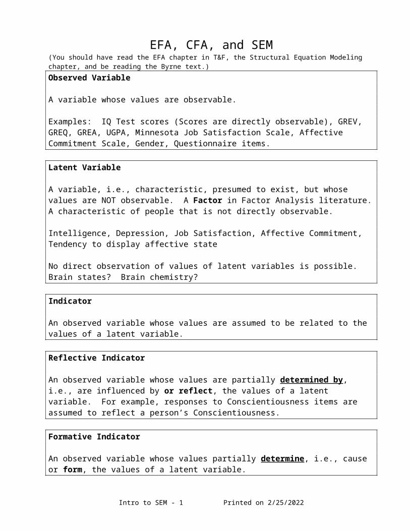
Path Diagrams of Analyses We’ve Done Previously

Following is how some of the analyses we’ve performed previously would be represented using path diagrams.

1. Simple correlation between two observed variables.

2. Simple correlations between three observed variables.

3. Simple regression of an observed dependent variable onto one observed independent variable.

4. Multiple Regression of an observed dependent variable onto three observed independent variables.


GRE-Q P511G eB or

GRE-V GRE-Q GRE-A

rVQ rQA

rVA

GRE-V GRE-Q

rVQ

GRE-Q P511G eBQ or Q

GRE-V

UPGA

BV or V

BU or U

Note that the endogenous variable is caused in part by catch-all influences.

Note that the endogenous variable is caused in part by catch-all influences.

ANOVA in SEM Models

Since ANOVA is simply regression analysis, the representation of ANOVA in SEM is merely as a regression analysis. The key is to represent the differences between groups with group coding variables, just as we did in 513 and in the beginning of 595 . . .

1) Independent Groups t-testThe two groups are represented by a single, dichotomous observed group-coding variable. It is the independent variable in the regression analysis.

2) One Way ANOVAThe K groups are represented by K-1 group-coding variables created using one of the coding schemes (although I recommend contrast coding). They are the independent variables in the regression analysis. If contrast codes are used, the correlations between all the group coding variables are 0, so no arrows between them need be shown.

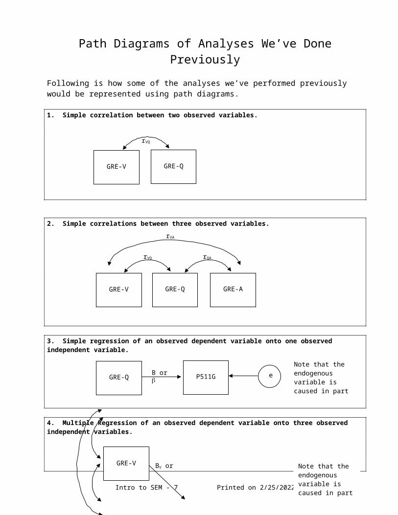
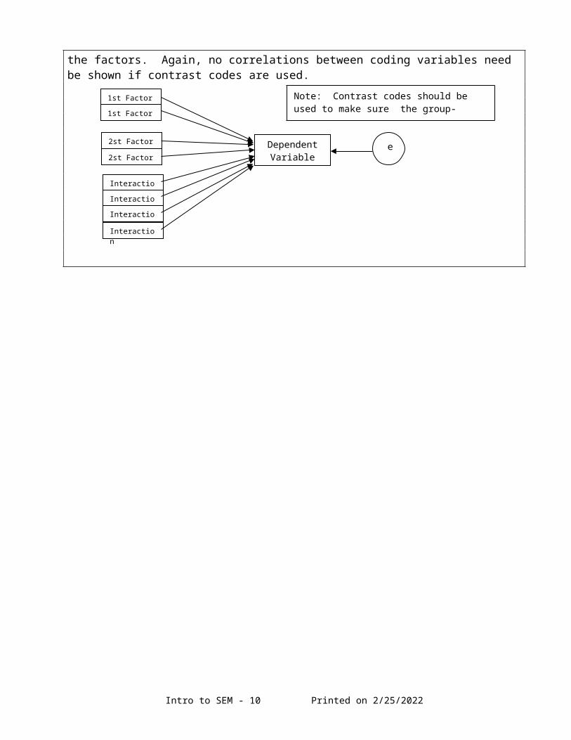
3) Factorial ANOVA.Each factor is represented by G-1 group-coding variables created using one of the coding schemes. The interaction(s) is/are represented by products of the group-coding variables representing the factors. Again, no correlations between coding variables need be shown if contrast codes are used.


Dichotomous variable representing the two groups

DependentVariable

e

1st Group-coding contrast code variable

2nd Group-coding contrast code variable.

(K-1)th Group-coding contrast code variable.

. . . . .

DependentVariable

e

1st Factor

1st Factor

2st Factor

2st Factor

Interaction

Interaction

Interaction

Interaction

DependentVariable

e

Note: Contrast codes were used so Group-coding variables are uncorrelated.

Note: Contrast codes should be used to make sure the group-coding variables uncorrelated.

Path Diagrams representing Exploratory Factor Analysis

1) Exploratory Factor Analysis solution with one factor.

The factor is represented by a latent variable with three or more observed indicators. (Three is the generally recommended minimum no. of indicators for a factor.)

Note that factors are exogenous. Indicators are endogenous. Since the indicators are endogenous, all of their variance must be accounted for by the model. Thus, each indicator must have an error latent variable to account for the variance in it not accounted for by the factor.

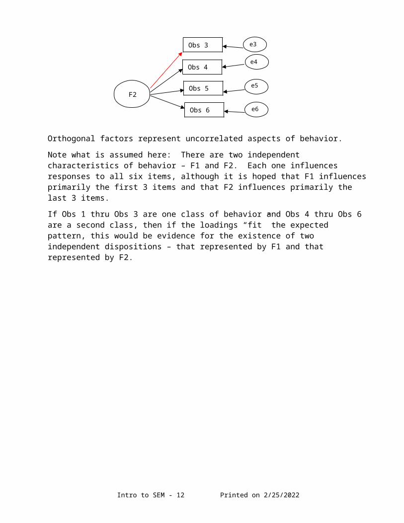
2) Exploratory Factor Analysis solution with two orthogonal factors.

Each factor is represented by a latent variable with three or more indicators. The orthogonality of the factors is represented by the fact that there is no arrow connecting the factor symbols.

Let’s assume that Obs1, 2, and 3 are thought to be primary indicators of F1 and 4,5,6 of F2.

For exploratory factor analysis, each variable is allowed to load on all factors. Of course, the hope is that the loadings will be substantial on only some of the factors and will be close to 0 on the others, but the loadings on all factors are retained, even if they’re close to 0. The loadings that might be close to 0 in the model are shown in red and orange.

Orthogonal factors represent uncorrelated aspects of behavior.

Note what is assumed here: There are two independent characteristics of behavior – F1 and F2. Each one influences responses to all six items, although it is hoped that F1 influences primarily the first 3 items and that F2 influences primarily the last 3 items.

If Obs 1 thru Obs 3 are one class of behavior and Obs 4 thru Obs 6 are a second class, then if the loadings “fit” the expected pattern, this would be evidence for the existence of two independent dispositions – that represented by F1 and that represented by F2.


Obs 1

Obs 2

Obs 3

Obs 4

Obs 5

Obs 6

e1

e2

e3

e4

e5

e6

F1

F2

Obs 1

Obs 2

Obs 3

e1

e2

e3

F

3) Exploratory Factor Analysis solution with two oblique factors.

Each factor is represented by a latent variable with three or more indicators. The obliqueness of the factors is represented by the fact that there IS an arrow connecting the factors.

Again, in exploratory factor analysis, all indicators load on all factors, even if the loadings are close to zero.

Exploratory factor analysis (EFA) programs, such as that in SPSS, always report estimates of all loadings.

This solution is potentially as important as the orthogonal solution, although in general, I think that researchers are more interested in independent dispositions than they are in correlated dispositions. But discovering why two dispositions are separate but still correlated is an important and potentially rewarding task.


F

Obs 1

Obs 2

Obs 3

Obs 4

Obs 5

Obs 6

e4

e5

e6

e7

e8

e9

F1

F2

Confirmatory vs Exploratory Factor AnalysisIn Exploratory Factor Analysis, the loading of every item on every factor is estimated. The analyst hopes that some of those loadings will be large and some will be small. An EFA two-orthogonal-factor model is represented by the following diagram.

Note that there are arrows (loadings) connecting each variable to each factor. We have no hypotheses about the loading values – we’re exploring – so we estimate all loadings and let them lead us. No EFA programs (except that in Mplus) allow you to specify or fix loadings to pre-determined values.

In contrast to the exploration implicit in EFA, a factor analysis in which some loadings are fixed at specific values is called a Confirmatory Factor Analysis. The analysis is confirming one or more hypotheses about loadings, hypotheses representing by our fixing them at specific (usually 0) values.

Unfortunately, EFA and CFA cannot be done using the same computer program except MPlus.

The problem is that all EFA programs except that in Mplus won’t allow some loadings to be fixed at predetermined values. And CFA programs, except Mplus canNOT estimate the above model. Amos and all CFA programs other than MPlus require that some of the loadings be fixed.

So, in many instances, you will have to employ both SPSS (for EFA) and AMOS (for CFA) in exploring the interrelations between variables and factors. Often, analysts will use an EFA program to estimate ALL loadings to all factors, then use an SEM program to perform a confirmatory factor analysis, fixing those loadings that were close to 0 in the EFA to 0 in the CFA.

Note that in the above confirmatory model, loadings of indicators 4-6 on F1 are fixed at 0, as are loadings of indicators 1-3 on F2. (The arrows are missing, therefore assumed to be zero.)


Obs 1

Obs 2

Obs 3

Obs 4

Obs 5

Obs 6

e4

e5

e6

e7

e8

e9

F1

F2

Obs 1

Obs 2

Obs 3

Obs 4

Obs 5

Obs 6

F2

F1

E1

E2

E3

E4

E5

E6

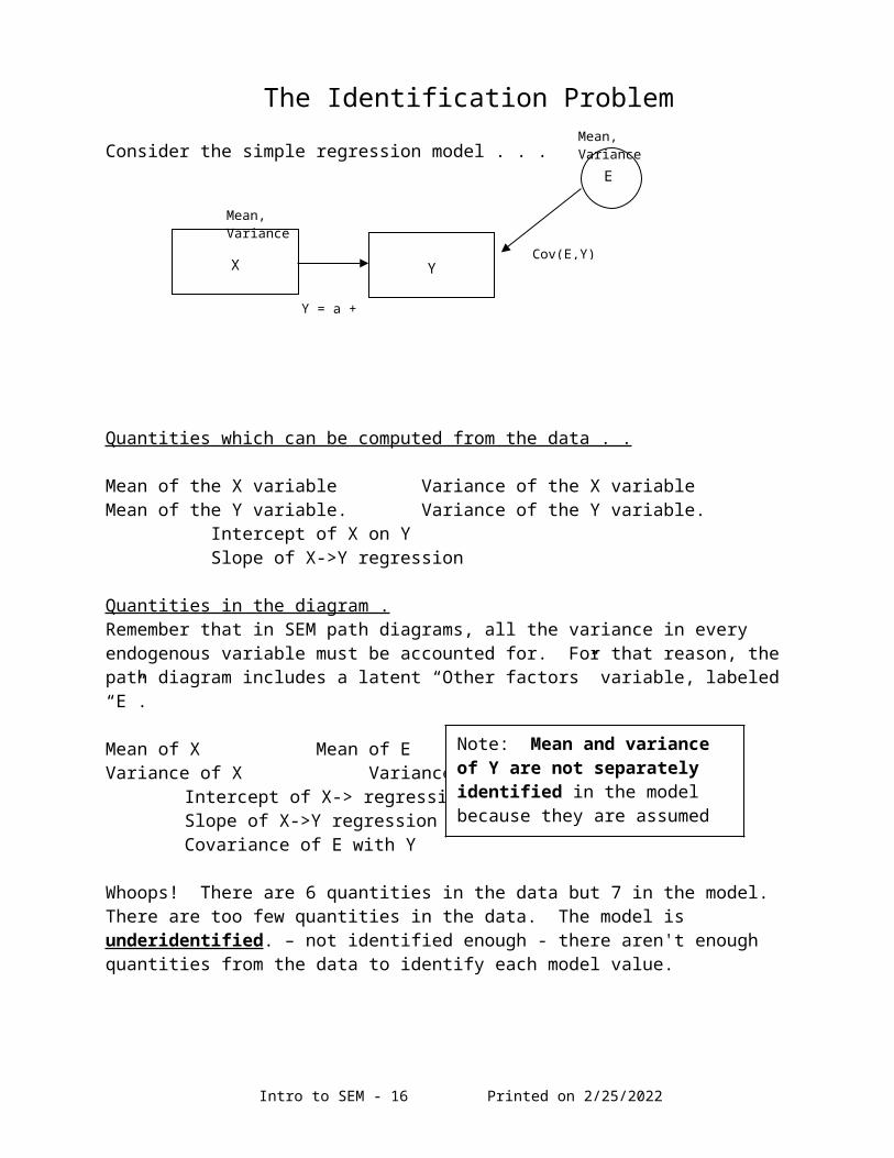
The Identification Problem

Consider the simple regression model . . .

Quantities which can be computed from the data . .

Mean of the X variable Variance of the X variableMean of the Y variable. Variance of the Y variable.

Intercept of X on YSlope of X->Y regression

Quantities in the diagram .Remember that in SEM path diagrams, all the variance in every endogenous variable must be accounted for. For that reason, the path diagram includes a latent “Other factors” variable, labeled “E”.

Mean of X Mean of EVariance of X Variance of E

Intercept of X-> regressionSlope of X->Y regressionCovariance of E with Y

Whoops! There are 6 quantities in the data but 7 in the model. There are too few quantities in the data. The model is underidentified. – not identified enough - there aren't enough quantities from the data to identify each model value.


X Y

E

Mean, Variance

Mean, Variance

Y = a + b*X

Cov(E,Y)

Note: Mean and variance of Y are not separately identified in the model because they are assumed to be completely determined by Y’s relationship to X and to E.

Dealing with underidentification . . .

The mean of E is always assumed to be 0.

1) Fix the variance of E to be 1.

So in this regression model, the path diagram will be

In this case, the model is said to be “just identified” or “completely identified”. This means that every estimable quantity in the model corresponds to one quantity obtained from the data.

Or,

2) Fix covariance of E with Y at 1.

Underidentified: Bad.

Just identified: OK

Overidentified: Great, you have degrees of freedom.


Y = a + b*X

Cov(E,Y)

X Y

E

Mean, Variance

Mean, Variance

1

Y=a+B*X

X Y

E

Mean, Variance

0, 1

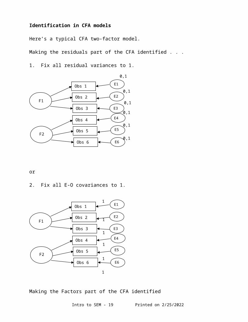
Identification in CFA models

Here’s a typical CFA two-factor model.

Making the residuals part of the CFA identified . . .

1. Fix all residual variances to 1.

or

2. Fix all E-O covariances to 1.

Making the Factors part of the CFA identified

1. Fix one of the loadings for each factor at 1Or2. Fix the variance of each factor at 1.


Obs 1

Obs 2

Obs 3

Obs 4

Obs 5

Obs 6

F2

F1

E1

E2

E3

E4

E5

E60,1

0,1

0,1

0,1

0,1

0,1

Obs 1

Obs 2

Obs 3

Obs 4

Obs 5

Obs 6

F2

F1

E1

E2

E3

E4

E5

E61

1

1

1

1

1

Examples

1. Fixing all variances.

2. Fixing residual loadings but Factor variances

3. Fixing residual loadings and factor loadings.


Obs 1

Obs 2

Obs 3

Obs 4

Obs 5

Obs 6

F2

F1

E1

E2

E3

E4

E5

E6

1

1

1

1

1

1

1

1

Obs 1

Obs 2

Obs 3

Obs 4

Obs 5

Obs 6

F2

F1

E1

E2

E3

E4

E5

E6

1

1

1

1

1

1

1

1

Obs 1

Obs 2

Obs 3

Obs 4

Obs 5

Obs 6

F2

F1

E1

E2

E3

E4

E5

E6

1

1

1

1

1

1

1

1

Programming with path diagrams: Introduction to Amos

Amos is an add-on program to SPSS that performs confirmatory factor analysis and structural equation modeling.

It is designed to emphasize a visual interface and has been written so that virtually all analyses can be performed by drawing path diagrams.

It also contains a text-based programming language for those who wish to write programs in the command language.

The Amos drawing toolkit with functions of the most frequently used tools.


Observed variable tool

Tool to draw latent variables

Tool to draw correlation arrows

Tool to draw regression arrows

Tool to select a single object

Tool to put text on the diagram

Tool to select all objects in diagram

Tool to deselect all objects in diagram

Tool to copy an object Tool to erase an object

Tool to move an object

Tool to tell Amos to run the diagram.

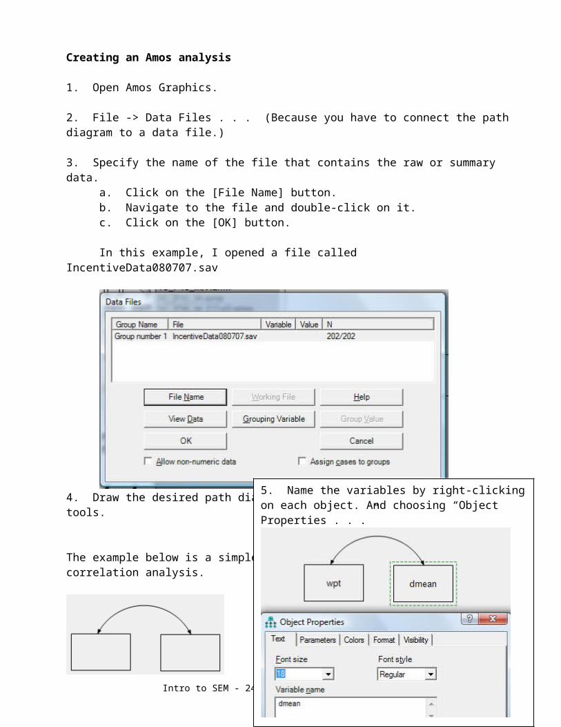
Creating an Amos analysis

1. Open Amos Graphics.

2. File -> Data Files . . . (Because you have to connect the path diagram to a data file.)

3. Specify the name of the file that contains the raw or summary data.a. Click on the [File Name] button.b. Navigate to the file and double-click on it.c. Click on the [OK] button.

In this example, I opened a file called IncentiveData080707.sav

4. Draw the desired path diagram using the appropriate drawing tools.

The example below is a simple correlation analysis.


5. Name the variables by right-clicking on each object. And choosing “Object Properties . . .”

Amos Details

For most of the analyses you’ll perform using Amos, you should get in the habit of doing the following . . .

View -> Analysis Properties -> Estimation

Check “Estimate means and intercepts”

View -> Analysis Properties -> Output

Check “Standardized estimates”Check “Squared multiple correlations”

Remember that you must fix some parameter values to make the models identified.


Doing old things in a new way: Analyses we’ve done before, now performed using AmosThe data used for this example are the VALDAT data. We’ll simply look at the output here. Later, we’ll focus on the menu sequences needed to get this output.

a. SPSS analysis of the correlation of FORMULA with P511G

Correlations

1.000 .502**.502** 1.000

. .000.000 .

83 7979 81

P511GFORMULAP511GFORMULAP511GFORMULA

PearsonCorrelation

Sig.(2-tailed)

N

P511G FORMULA

Correlations

Correlation is significant at the 0.01 level(2-tailed).

**.

b. Amos Input Path Diagram - Input Parameter Values (Note, I told Amos to estimate means for this analysis.)

c. Amos Output Path Diagram - Unstandardized (Raw) coefficients

c. Amos Path Diagram - Standardized coefficients


All variables are exogenous.

The mean and variance of Formula.

The mean and variance of p511g.

The correlation of p511g and Formula.

Means and variances of standardized variables are not displayed, since they are 0 and 1 respectively.

The covariance of p511g and Formula.

Simple Regression Analysis: SPSS and Amos

The data used here are the VALDAT data.

a. SPSS Version 10 output

GET FILE='E:\MdbT\P595\Amos\valdatnm.sav'..REGRESSION /MISSING LISTWISE /STATISTICS COEFF OUTS R ANOVA /CRITERIA=PIN(.05) POUT(.10) /NOORIGIN /DEPENDENT p511g /METHOD=ENTER formula .

RegressionVariables Entered/Removedb

FORMULAa . EnterModel1

VariablesEntered

VariablesRemoved Method

All requested variables entered.a.

Dependent Variable: P511Gb.

Model Summary

.480a .230 .220 4.725E-02Model1

R R SquareAdjustedR Square

Std. Error ofthe Estimate

Predictors: (Constant), FORMULAa.

ANOVAb

5.005E-02 1 5.005E-02 22.420 .000a

.167 75 2.233E-03

.217 76

RegressionResidualTotal

Model1

Sum ofSquares df Mean Square F Sig.

Predictors: (Constant), FORMULAa.

Dependent Variable: P511Gb.

Coefficientsa

.496 .078 6.361 .0003.004E-04 .000 .480 4.735 .000

(Constant)FORMULA

Model1

B Std. Error

UnstandardizedCoefficients

Beta

Standardized

Coefficients

t Sig.

Dependent Variable: P511Ga.


b. Amos Input Path Diagram - Input parameter values

c. Amos Output Path Diagram - Unstandardized (Raw) coefficients

Mean of X Variance of X

d. Amos Output Path Diagram - Standardized coefficients(View/Set -> Analysis Properties -> Output to get Amos to print Standardized estimates what a pain!!)

Note that .482 + .882 = 1. All of variance of p511g has been accounted for. We say that formula and error partition the total variance of p511g.


The model is underidentified unless you fix the value of one parameter. Fix either the variance of the latent error variable to 1 or the regression weight to 1. Here, the variance has been fixed.

Note that the fixed parameter values were not changed.

For what it's worth, the estimated unstandardized (raw score) relationship of p511g to the “other factors” latent variable.

The estimated unstandardized (raw score) relationship of p511g .to Formula - the slope, to 2 decimal places.

Variance of Formula.

Correlation of p511g with latent “other factors”..= sqrt(1-r2)=sqrt(1-.482) = sqrt(1-.23) = sqrt(.77)=.88

Correlation of p511g with Formula.

r2 for the model. You may have to pull down [View/Set] -> Analysis Properties -> Output to ask for this to be printed.

Two IV Regression Example - SPSS and Amos

The data here are the VALDATnm data. UGPA and GREQ are predictors of P511G.

a. SPSS output.GET FILE='G:\MdbT\P595\P595AL09-Amos\valdatnm.sav'.DATASET NAME DataSet1 WINDOW=FRONT.REGRESSION /DESCRIPTIVES MEAN STDDEV CORR SIG N /MISSING LISTWISE /STATISTICS COEFF OUTS R ANOVA /CRITERIA=PIN(.05) POUT(.10) /NOORIGIN /DEPENDENT p511g /METHOD=ENTER ugpa greq .

Regression[DataSet1] G:\MdbT\P595\P595AL09-Amos\valdatnm.sav

Correlations

1.000 .225 .322

.225 1.000 -.262

.322 -.262 1.000

. .025 .002

.025 . .011

.002 .011 .

77 77 77

77 77 77

77 77 77

p511g

ugpa

greq

p511g

ugpa

greq

p511g

ugpa

greq

PearsonCorrelation

Sig. (1-tailed)

N

p511g ugpa greq

Variables Entered/Removed b

greq, ugpa a . EnterModel1

Variables EnteredVariablesRemoved Method


Dependent Variable: p511gb.

Model Summary

.455a .207 .185 .04828Model1

R R Square Adjusted R SquareStd. Error ofthe Estimate

Predictors: (Constant), greq, ugpaa.

Coefficients a

.571 .069 8.228 .000

.048 .016 .332 3.098 .003

.000 .000 .410 3.817 .000

(Constant)

ugpa

greq

Model1

B Std. Error

Unstandardized Coefficients

Beta

StandardizedCoefficients

t Sig.

Dependent Variable: p511ga.


b. Amos Input Path Diagram - Input parameters.

c. Amos Output Path Diagram - Unstandardized (Raw) coefficientsI forgot to check “Estimate means and intercepts, so no means are printed.)


Raw Regression coefficient relating p511g to residual effects.

Raw partial regression coefficient relating p511g to ugpa

Raw regression coefficient relating p511g to Formula. (Zero to two decimal places.)

The variance of the (unobserved) error latent variable must be specified at 1.

Note that if the IVs are correlated, you must specify that they are correlated. Otherwise, Amos will perform the analysis assuming they're uncorrelated.

Raw partial regression coefficient relating p511g to GREQ to 2 decimal places.

Covariance of ugpa and greq.

Variance of ugpa

d. Amos Output Path Diagram - Standardized coefficients.

Note that .332 + .412 + .892 = 1.07 > 1.0. This is because r2s partition variance only when variables are uncorrelated.e. Amos Text Output - Details of input and minimizationChi-square = 0.000Degrees of freedom = 0Probability level cannot be computedMaximum Likelihood Estimates----------------------------Regression Weights: Estimate S.E. C.R. Label ------------------- -------- ------- ------- -------

p511g <----- ugpa 0.048 0.015 3.140 p511g <---- error 0.047 0.004 12.329 p511g <----- greq 0.000 0.000 3.869

Standardized Regression Weights: Estimate-------------------------------- --------

p511g <----- ugpa 0.332 p511g <---- error 0.891 p511g <----- greq 0.410

Covariances: Estimate S.E. C.R. Label ------------ -------- ------- ------- -------

ugpa <-----> greq -8.537 3.861 -2.211

Correlations: Estimate------------- --------

ugpa <-----> greq -0.262

Variances: Estimate S.E. C.R. Label ---------- -------- ------- ------- -------

error 1.000 ugpa 0.134 0.022 6.164 greq 7897.622 1281.163 6.164

Squared Multiple Correlations: Estimate------------------------------ --------

p511g 0.207


Standardized partial regression coefficients.

Correlation of ugpa and greq.

Multiple R2.

SQRT(1-R2)=sqrt(1-.21) = sqrt(.79)=.89

Note – No overall test of significance of R2.This test is available in the ANOVA box in SPSS.

Oneway Analysis of Variance Example - SPSS and Amos

The data for this example follow. They're used to introduce the 595 students to contrast coding. The dependent variable is Job Satisfaction (JS). The research factor is Job, with three levels. It is contrast coded by CC1 and CC2.

The data for this example are in ‘MdbT\P595\Amos\ OnewayegData.sav’

ID JS JOB CC1 CC2

1 6 1 .667 .000 2 7 1 .667 .000 3 8 1 .667 .000 4 11 1 .667 .000 5 9 1 .667 .000 6 7 1 .667 .000 7 7 1 .667 .000 8 5 2 -.333 .500 9 7 2 -.333 .500 10 8 2 -.333 .500 11 9 2 -.333 .500 12 10 2 -.333 .500 13 8 2 -.333 .500 14 9 2 -.333 .500 15 4 3 -.333 -.500 16 3 3 -.333 -.500 17 6 3 -.333 -.500 18 5 3 -.333 -.500 19 7 3 -.333 -.500 20 8 3 -.333 -.500 21 2 3 -.333 -.500

a. SPSS Oneway output.

OnewayANOVA

JS

40.095 2 20.048 5.930 .011

60.857 18 3.381

100.952 20

BetweenGroups

Within Groups

Total



The rule for forming a contrast variable between two sets of groups is

1st Value = No. of groups in 2nd set / Total no. of groups.

2nd Value= - No. of groups in 1st set / Total no. of groups.

3rd Value = 0 for all groups to be excluded.

So, 1st Value of CC1 = 2 / 3 = .667.

2nd Value of CC1 = - 1 / 3

1st Value of CC2 = 1 / 2 = .5

2nd Value of CC2 = -1 / 2 = -..5

3rd Value of CC2 = 0 to exclude Job 1.

b. SPSS Regression Output.

regression variables = js cc1 cc2 /dependent = js /enter.

RegressionVariables Entered/Removed b

CC2, CC1 a . EnterModel1

VariablesEntered

VariablesRemoved Method


Dependent Variable: JSb.

Model Summary

.630a .397 .330 1.8387Model1

R R SquareAdjusted R

SquareStd. Error ofthe Estimate

Predictors: (Constant), CC2, CC1a.

ANOVA b

40.095 2 20.048 5.930 .011a

60.857 18 3.381

100.952 20

Regression

Residual

Total

Model1


Predictors: (Constant), CC2, CC1a.

Dependent Variable: JSb.

Coefficients a

6.952 .401 17.326 .000

1.357 .851 .292 1.594 .128

3.000 .983 .559 3.052 .007

(Constant)

CC1

CC2

Model1

B Std. Error

Unstandardized Coefficients

Beta

StandardizedCoefficients

t Sig.

Dependent Variable: JSa.


c. Amos Input Path Diagram.

d. Amos Output Path Diagram - Unstandardized (Raw) Coefficients

e. Amos Output Path Diagram - Standardized Coefficients


Note that the correlation between group coding variables must be estimated. It's zero here because they're contrast codes.

This was prepared using Amos 3.6. I chose the "Estimate means" option. This was not required, but it caused means to be displayed.

InterceptMean and variance.

Note that .292 + .562 + .782 = 1.01 ~~ 1.r2s partition variance since the variables are all independent.

Multiple R2

f. Amos Text Output - Results

Result (Default model)Minimum was achievedChi-square = .00000Degrees of freedom = 0Probability level cannot be computedMaximum Likelihood EstimatesRegression Weights: (Group number 1 - Default model)

Estimate S.E. C.R. P

Label

JS <--- CC1 1.35714 .80749 1.68069 .09282JS <--- CC2 3.00000 .93241 3.21747 .00129

Standardized Regression Weights: (Group number 1 - Default model)Estimate

JS <--- CC1 .29179JS <--- CC2 .55859

Means: (Group number 1 - Default model)Estimate S.E. C.R. P Label

CC1 .00033 .10541 .00316 .99748CC2 .00000 .09129 .00000 1.00000

Intercepts: (Group number 1 - Default model)Estimate S.E. C.R. P Label

JS 6.95193 .38065 18.26308 ***

Covariances: (Group number 1 - Default model)


Coefficients Box – B coefficients only

Coefficients Box – Standardized coefficients

Descriptive statistics

Coefficients box - Constant

Estimate S.E. C.R. P LabelCC1 <--> CC2 .00000 .04303 .00000 1.00000

Correlations: (Group number 1 - Default model)Estimate

CC1 <--> CC2 .00000

Variances: (Group number 1 - Default model)Estimate S.E. C.R. P Label

CC1 .22222 .07027 3.16228 .00157CC2 .16667 .05270 3.16228 .00157resid 2.89796 .91642 3.16228 .00157

Squared Multiple Correlations: (Group number 1 - Default model)Estimate

JS .39717


Note that AMOS does not provide a test of the null hypothesis that in the population, the multiple R = 0. This test is provided in the ANOVA box in SPSS.

Model summary

Not in SPSS

Descriptive statistics

Documents

Diagrams Representing Relationships between …web2.utc.edu/~pbv184/PSY595/L8 - EFA, CFA, and SEM.doc · Web viewREGRESSION /DESCRIPTIVES MEAN STDDEV CORR SIG N /MISSING LISTWISE