Diagrammatic &Graphical Presentation of Data

Amity Business School

Lecture 2 : Diagrammatic & Graphical

Presentation of Data

Department of Decision Sciences


Objective of the Lecture

To introduce diagrammatic and graphical statistical methods that

allows managers to summarize data visually to produce useful

information.

To understand the importance of the graphical methods commonly

used to summarize both qualitative and quantitative data.

To know how they are prepared and how they should be

interpreted.


Introduction The most common and simple forms of pictorial representation of

data are:

(i) Bar diagram

(ii) Histogram

(iii) Pie diagram

(iv) Stem-Leaf display

(v) Frequency Polygon

(vi) Ogive

Though the first two approaches above are similar in nature, the bar

diagram is meant for categorical data whereas the histogram and

stem-leaf display are meant solely for quantitative data. On the

other hand, pie diagram can be used for both types of data.


Example 1.1: University Placement Office Survey

The student placement office at a university conducted a survey of

last year's business school graduates to determine the general areas

in which the graduates found jobs. The placement office intended to

use the resulting information to help decide where to concentrate

its efforts in attracting companies to campus to conduct job

interviews. Each graduate was asked in which area he or she found

a job. The areas of employment are

Accounting

Finance

General management

Marketing/Sales

Other


The responses were recorded using the codes 1, 2, 3, 4, find 5,

respectively. Construct a frequency and relative frequency

distribution for these data and graphically summarize the data by

producing a bar chart and a pie chart.

Data on the next slide…


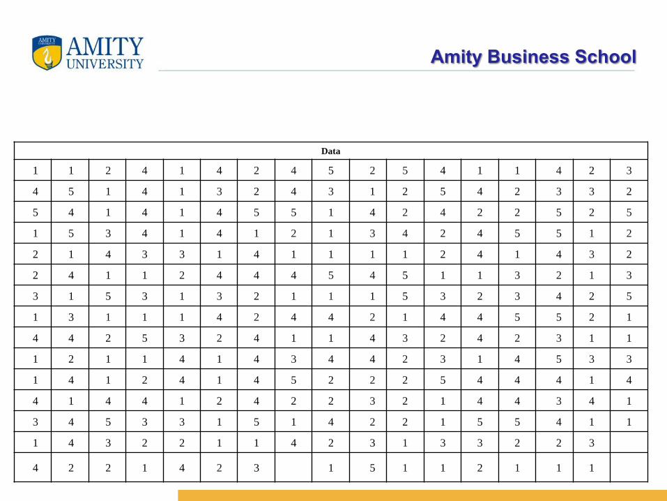
Data

1 1 2 4 1 4 2 4 5 2 5 4 1 1 4 2 3

4 5 1 4 1 3 2 4 3 1 2 5 4 2 3 3 2

5 4 1 4 1 4 5 5 1 4 2 4 2 2 5 2 5

1 5 3 4 1 4 1 2 1 3 4 2 4 5 5 1 2

2 1 4 3 3 1 4 1 1 1 1 2 4 1 4 3 2

2 4 1 1 2 4 4 4 5 4 5 1 1 3 2 1 3

3 1 5 3 1 3 2 1 1 1 5 3 2 3 4 2 5

1 3 1 1 1 4 2 4 4 2 1 4 4 5 5 2 1

4 4 2 5 3 2 4 1 1 4 3 2 4 2 3 1 1

1 2 1 1 4 1 4 3 4 4 2 3 1 4 5 3 3

1 4 1 2 4 1 4 5 2 2 2 5 4 4 4 1 4

4 1 4 4 1 2 4 2 2 3 2 1 4 4 3 4 1

3 4 5 3 3 1 5 1 4 2 2 1 5 5 4 1 1

1 4 3 2 2 1 1 4 2 3 1 3 3 2 2 3

4 2 2 1 4 2 3 1 5 1 1 2 1 1 1


Scanning the data produces no real information. To extract the

information requires the application of a statistical or graphical

technique. To choose the appropriate technique we must first

identify the type of data. In this example the data are nominal

because the numbers represent categories. The only calculation

permitted on nominal data is to count the number of occurrences of

each category. The list of the categories and their count constitute

the frequency distribution. The relative frequency distribution is

produced by converting the frequencies into proportion. The

frequency and relative frequency distributions are combined in

Table 1.1


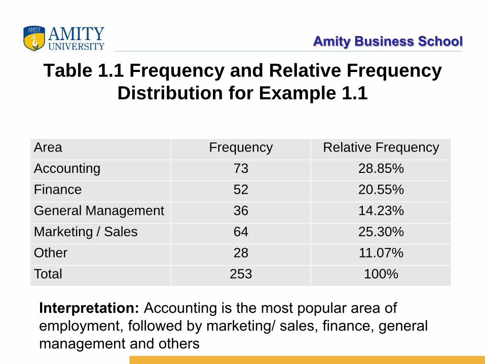
Table 1.1 Frequency and Relative Frequency

Distribution for Example 1.1

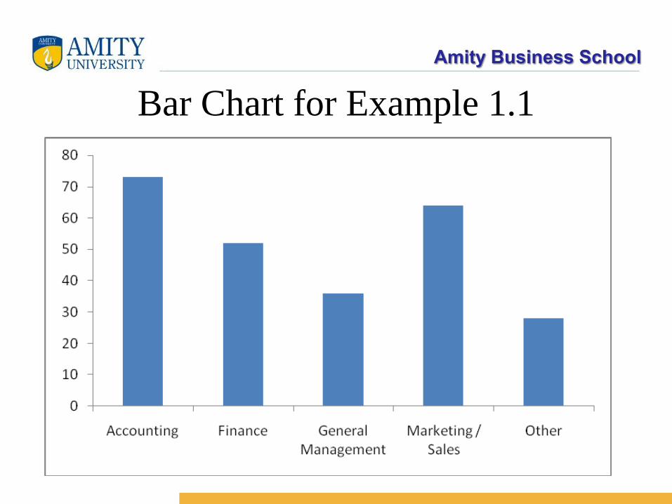
Area Frequency Relative Frequency

Accounting 73 28.85%

Finance 52 20.55%

General Management 36 14.23%

Marketing / Sales 64 25.30%

Other 28 11.07%

Total 253 100%

Interpretation: Accounting is the most popular area of

employment, followed by marketing/ sales, finance, general

management and others


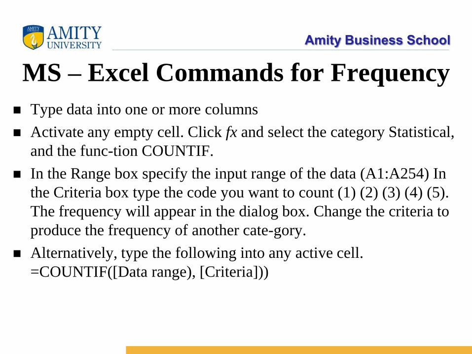
MS – Excel Commands for Frequency

Type data into one or more columns

Activate any empty cell. Click fx and select the category Statistical,

and the function COUNTIF.

In the Range box specify the input range of the data (A1:A254) In

the Criteria box type the code you want to count (1) (2) (3) (4) (5).

The frequency will appear in the dialog box. Change the criteria to

produce the frequency of another category.

Alternatively, type the following into any active cell.

=COUNTIF([Data range), [Criteria]))


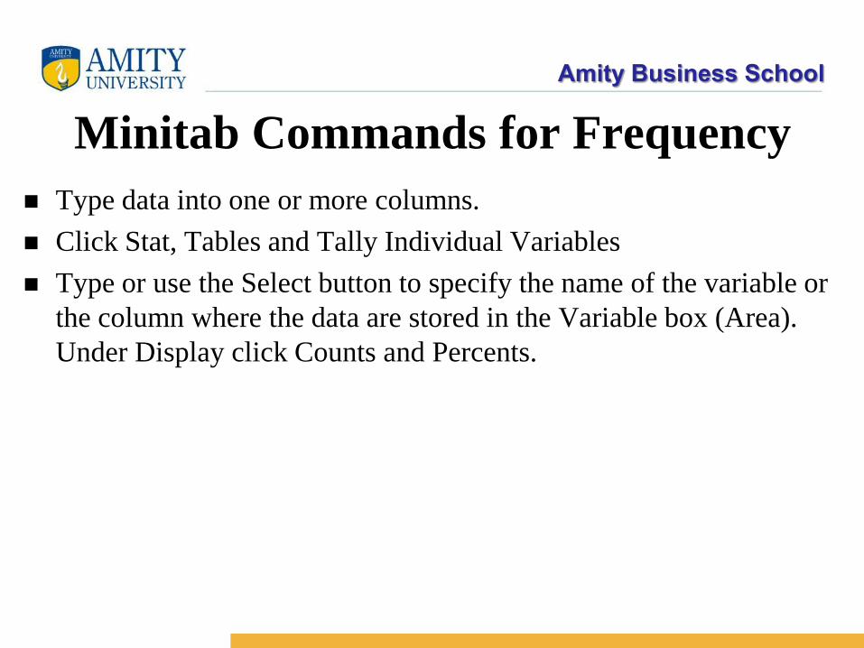
Minitab Commands for Frequency

Type data into one or more columns.

Click Stat, Tables and Tally Individual Variables

Type or use the Select button to specify the name of the variable or

the column where the data are stored in the Variable box (Area).

Under Display click Counts and Percents.


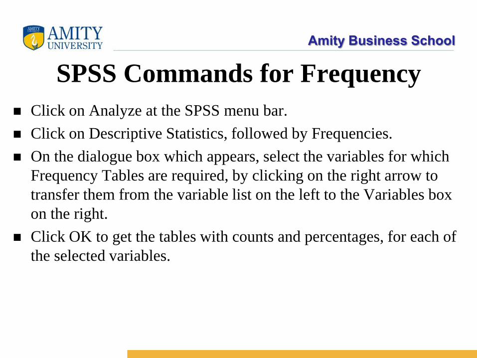
SPSS Commands for Frequency

Click on Analyze at the SPSS menu bar.

Click on Descriptive Statistics, followed by Frequencies.

On the dialogue box which appears, select the variables for which

Frequency Tables are required, by clicking on the right arrow to

transfer them from the variable list on the left to the Variables box

on the right.

Click OK to get the tables with counts and percentages, for each of

the selected variables.


Bar and Pie Chart

Graphical techniques generally catch a reader's eye more quickly

than does a table of numbers. Two graphical techniques can be used

to display the results shown in the table. A bar chart is often used to

display frequencies; a pie chart graphically shows relative

frequencies.


Bar Chart for Example 1.1


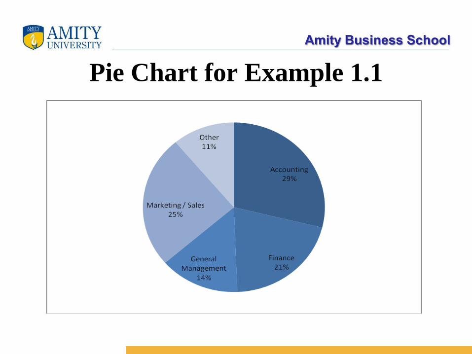
Pie Chart

If we wish to emphasize the relative frequencies instead of drawing

the bar chart, we draw the pie chart. A pie chart is simply a circle

subdivided into slices that represent the categories. It is drawn so

that the size of each slice is proportional to the percentage

corresponding to that category. For example, since the entire circle

is composed of 360 degrees, a category that contains 25% of the

observations is represented by a slice of the pie that contains 25%

of 360 degrees, which is equal to 90 degrees. The number of

degrees for each category in Example 1.1 is shown in Table 1.2.


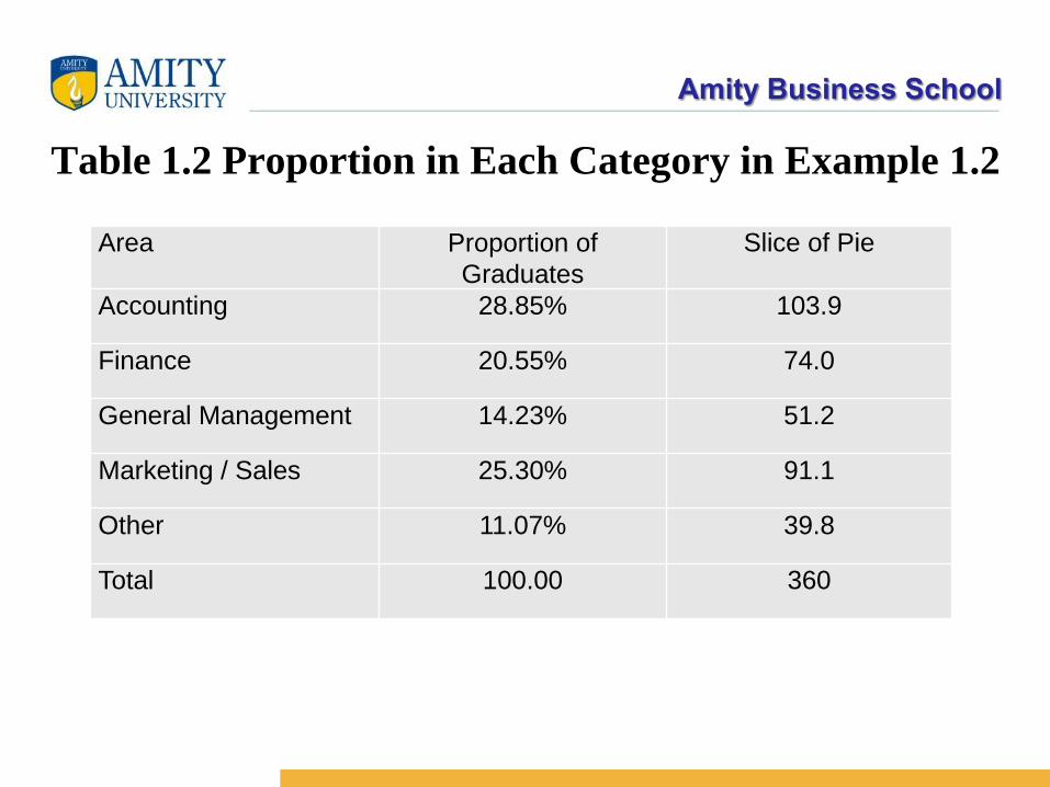
Table 1.2 Proportion in Each Category in Example 1.2

Area Proportion of

Graduates

Slice of Pie

Accounting 28.85% 103.9

Finance 20.55% 74.0

General Management 14.23% 51.2

Marketing / Sales 25.30% 91.1

Other 11.07% 39.8

Total 100.00 360


Pie Chart for Example 1.1


MS – Excel Commands for Bar and Pie Chart

After creating the frequency distribution, highlight the column of

frequencies.

For a bar chart click the Chart Wizard, Column and Finish. For a

pie chart click Pie instead of Column.

Click Chart (on Tool Bar), Chart Options. and make whatever

changes you think

make the chart look best.


Minitab Commands for Bar and Pie ChartFor a bar chart:

Click Graph and Bar Chart.

In the Bars represent box click Counts of unique values and select Simple.

Type or use the Select button to specify the variable in the Variables box

(Area).

We clicked Labels and added the title and clicked Data Labels and use y-

value labels to display the frequencies at the top of the columns.

For a pie chart:

Click Graph and Pie Chart.

Click Chart raw data and in the Categorical variables box type or use the

Select button to specify the variable (Area).

We clicked Labels and added the title. We clicked Slice Labels and

clicked Category name and Percent.


SPSS Commands for Bar and Pie Chart


Click on Descriptive Statistics, followed by Frequencies.

On the dialogue box which appears, select the variables for which

Frequency Tables are required, by clicking on the right arrow to transfer

them from the variable list on the left to the Variables box on the right.

Click OK to get the tables with counts and percentages, for each of the

selected variables.

Charts can be requested by clicking on Charts on the main dialogue box,

selecting the required type of charts, and clicking Continue before step 4

above.

Alternatively : click on Graphs at the SPSS menu bar followed by Chart

Builder


Histogram

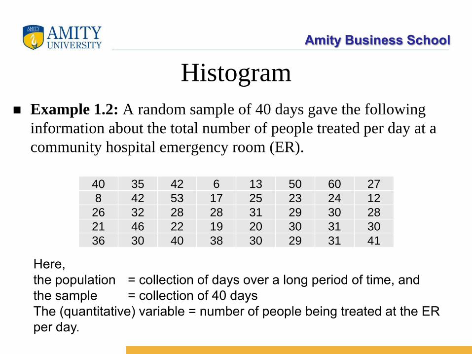
Example 1.2: A random sample of 40 days gave the following

information about the total number of people treated per day at a

community hospital emergency room (ER).

40 35 42 6 13 50 60 27

8 42 53 17 25 23 24 12

26 32 28 28 31 29 30 28

21 46 22 19 20 30 31 30

36 30 40 38 30 29 31 41

Here,

the population = collection of days over a long period of time, and

the sample = collection of 40 days

The (quantitative) variable = number of people being treated at the ER

per day.


Since the variable is quantitative and can take many possible values

(much more than a typical categorical variable), it does not make

sense to have frequencies for distinct entries (we might end up with

40 distinct entries with each having frequency 1). So, here we first

find the minimum (min) and maximum (max) entries to get a spread

of the variable (in the sample).

There is a systematic way of finding the min and max. First, find

the min and max for each column, which is easy to do, since there

are much fewer entries in a single column (compared to the whole

array). Next, find,


(overall) min = minimum of column minimums

and

(overall) max = maximum of column maximums.

By this method, we get

Column minimums = 8, 30, 22, 6, 13, 23, 24 and 12;

Column maximums = 40,46,53,38,31,50,60 and 41;

and hence

min = 6 and max = 60


Note that the unit here (i.e., the smallest possible increment of the

quantitative variable) is 1 (or 1 patient). We modify the range (6,

60) by extending by one half of a unit on both sides. This called a

modified range and for the present data set, our modified range is

(5.5, 60.5). The lower limit of the modified range is 5.5, and the

upper limit is 60.5. The idea behind the modified range is that it

includes the boundary values (6 and 60) properly. The length (L) of

the modified range is

L = upper limit – lower limit

= 60.5 – 5.5 = 55


This length L is now divided into several subintervals which gives

us a few classes. The number of classes, say k, is a convenient

number, usually taken between 5 and 8. For the present case take k

= 5 and then

l = length of each class = L/k = 11

(The notation l is used to denote the length of each class or sub

interval)

Therefore, we can divide the modified range (5.5, 60.5) into

successive contiguous classes: (5.5, 5.5 + l) = (5.5, 16.5), (16.5,

16.5 + l) = (16.5, 27.5), (27.5, 27.5 + l) = (27.5, 38.5), (38.5, 38.5 +

l) = (38.5, 49.5) and (49.5, 49.5 + l) = (49.5, 60.5).


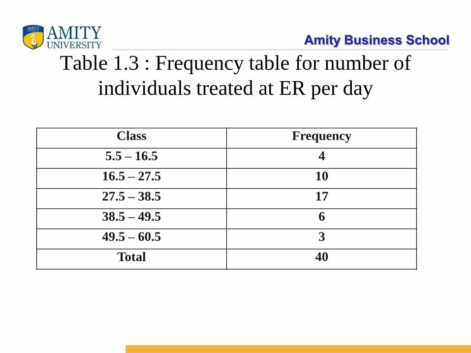
Table 1.3 : Frequency table for number of

individuals treated at ER per day

Class Frequency

5.5 – 16.5 4

16.5 – 27.5 10

27.5 – 38.5 17

38.5 – 49.5 6

49.5 – 60.5 3

Total 40


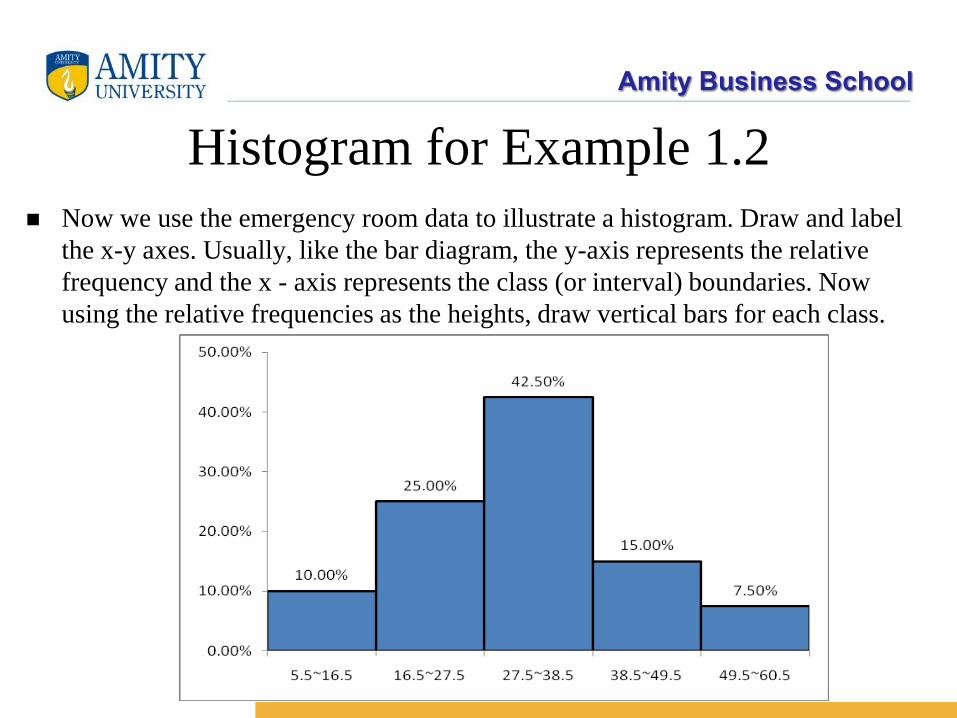
Histogram for Example 1.2

Now we use the emergency room data to illustrate a histogram. Draw and label

the x-y axes. Usually, like the bar diagram, the y-axis represents the relative

frequency and the x - axis represents the class (or interval) boundaries. Now

using the relative frequencies as the heights, draw vertical bars for each class.


Given a frequency table (with fixed number of classes and class

boundaries), the histogram of a dataset is unique (unlike the bar

diagram). This is due to the natural ordering of the classes. Another

departure from the bar diagram is the absence of fixed gap between

two successive classes.

A bar graph and a histogram are essentially the same thing; both are

graphical presentations of the data in a frequency distribution. A

histogram is just a bar graph with no separation between bars. The

separation between bars is appropriate for qualitative data because

the data are discrete; no intermediate values are possible. For

discrete quantitative data, a separation between bars is also

appropriate.


Frequency Polygon Histogram gives rise to another simple concept called relative

frequency polygon. Find the midpoint of each class (midpoint of a

class is found by adding the two endpoints of the class and then

dividing by 2), and then plot the relative frequencies (on y-axis)

against the midpoints (on x-axis). Connect the adjacent points with

straight line segments, and the resultant diagram is a frequency

polygon. A frequency polygon shows the trend in the data in terms of

frequency (which is also evident in the histogram).

From the frequency polygon in Figure 1.3 it is clear that for the

emergency room dataset, the frequency or relative frequency increases

as the number of patients per day increases to 33, and beyond this the

frequency starts falling. Roughly, we see that there are more days

when we treat 25 patients per day than 15 patients per day. Similarly,

less number of days treat 45 patients per day than 35 patients per day.


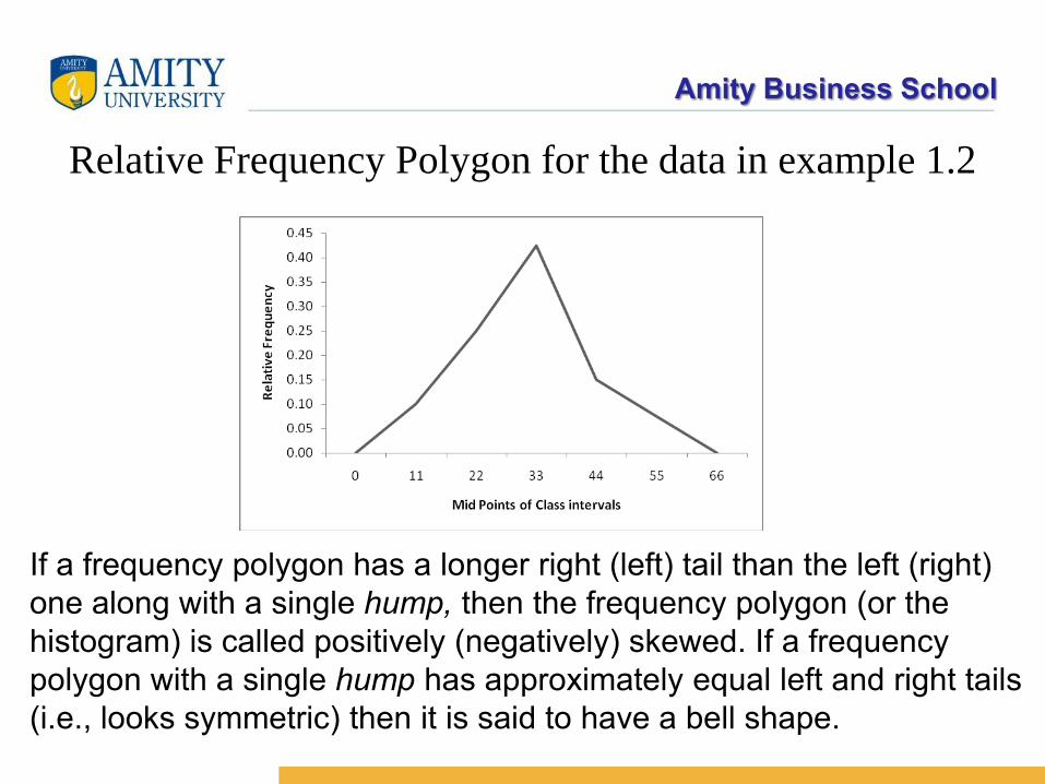
Relative Frequency Polygon for the data in example 1.2

If a frequency polygon has a longer right (left) tail than the left (right)

one along with a single hump, then the frequency polygon (or the

histogram) is called positively (negatively) skewed. If a frequency

polygon with a single hump has approximately equal left and right tails

(i.e., looks symmetric) then it is said to have a bell shape.


MS Excel Commands for Histogram

Type the data into one column. In another column type the upper limits of the

class intervals. Excel calls them bins

Clicks Tool, Data Analysis …, and Histogram. If Data Analysis does not appear

in the menu box, you have to install it by using Excel Options and Add ins.

Specify the Input Range and the Bin Range. Click Chart Output. Click Labels if

the first row contains names.

To remove the gaps place the cursor over one of the rectangles-and click the right

button of the mouse. Click (with the left button) Format Data Series .... Click

Options, move the pointer to Gap Width and change the number from 150 to O.

Click Chart and Chart Options ... to make cosmetic changes.

Note that the numbers along the horizontal axis represent the upper limits of each

class although they appear to be placed in the centers. Except for the first class,

Excel counts the number of observations in each class that are greater than the

lower limit and less than or equal to the upper limit.


Minitab Commands for Histogram

Note that Minitab counts the number of observations in each class that are

strictly less than the upper limit and greater than or equal to the lower

limit.

Type or import the data into one column.

Click Graph, Histogram ... , and Simple.

Type or use the Select button to specify the name of the variable in the

Graph variables box . Click Data View.

Click Data Display and Bar. Minitab will create a histogram using its own

choices of class intervals.

To choose your own classes, double-click the horizontal axis. Click

Binning.

Under Interval Type choose Cutpoint. Under Interval Definition choose

Midpoint/Cutpoint positions and type in your choices.


Stem and Leaf Display

The stem-leaf display is an extremely useful way of studying data

structure for a quantitative variable. A frequency table and the

corresponding histogram provide a useful organization and pictorial

representation of data. However, in a frequency table (like Table

2.6) we do lose individual values of the observations. A stem-leaf

display is a simple device that groups the whole dataset and

produces a histogram or bar diagram like picture, yet allows us to

recover the original dataset if required. We illustrate this with the

following example.


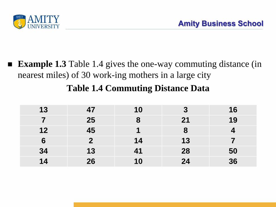
Example 1.3 Table 1.4 gives the one-way commuting distance (in

nearest miles) of 30 working mothers in a large city

Table 1.4 Commuting Distance Data

13 47 10 3 16

7 25 8 21 19

12 45 1 8 4

6 2 14 13 7

34 13 41 28 50

14 26 10 24 36


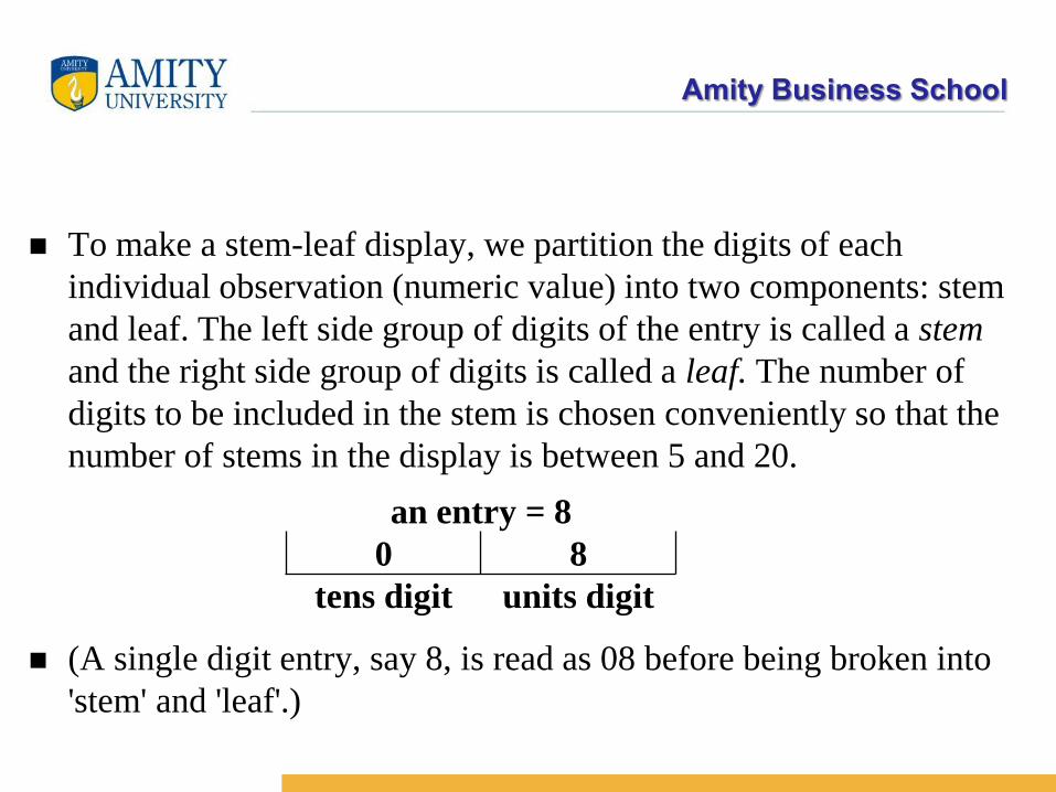
To make a stem-leaf display, we partition the digits of each

individual observation (numeric value) into two components: stem

and leaf. The left side group of digits of the entry is called a stem

and the right side group of digits is called a leaf. The number of

digits to be included in the stem is chosen conveniently so that the

number of stems in the display is between 5 and 20.

(A single digit entry, say 8, is read as 08 before being broken into

'stem' and 'leaf'.)

an entry = 8

0 8

tens digit units digit


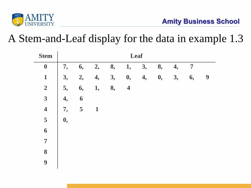
For the data in Table 1.4, where all entries are one- or two-digit

numbers, we use tens digit of an entry to form the stem and the

units digit to form the corresponding leaf. For the first entry 13, the

stem is 1 and the leaf is 3. The entry 8 is treated as 08, meaning 0

for its stem and 8 for its leaf. Figure 1.5 gives the stem-leaf display

of the above mentioned data. From Figure 1.5, it is clear that most

of the entries are in the l0-mile range [i.e., (10, 19) miles], followed

by the 0-mile range [i.e., (0, 9) miles]. The horizontal length of the

leaves represents the frequency for the corresponding stem which is

essentially a class. The stem 1 represents the class 10-19 miles, or

more correctly the class 9.5-19.5 miles, since the data entries are

rounded values and hence anyone commuting 9.5 (or 9.6 or 9.7 or

9.8 or 9.9) miles would be assigned the value 10.


A Stem-and-Leaf display for the data in example 1.3

Stem Leaf

0 7, 6, 2, 8, 1, 3, 8, 4, 7

1 3, 2, 4, 3, 0, 4, 0, 3, 6, 9

2 5, 6, 1, 8, 4

3 4, 6

4 7, 5 1

5 0,

6

7

8

9


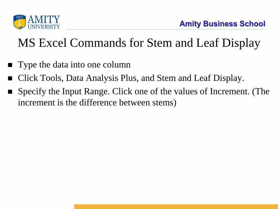
MS Excel Commands for Stem and Leaf Display

Type the data into one column

Click Tools, Data Analysis Plus, and Stem and Leaf Display.

Specify the Input Range. Click one of the values of Increment. (The

increment is the difference between stems)


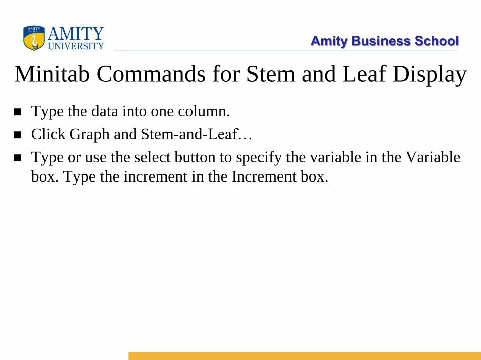
Minitab Commands for Stem and Leaf Display

Type the data into one column.

Click Graph and Stem-and-Leaf…

Type or use the select button to specify the variable in the Variable

box. Type the increment in the Increment box.


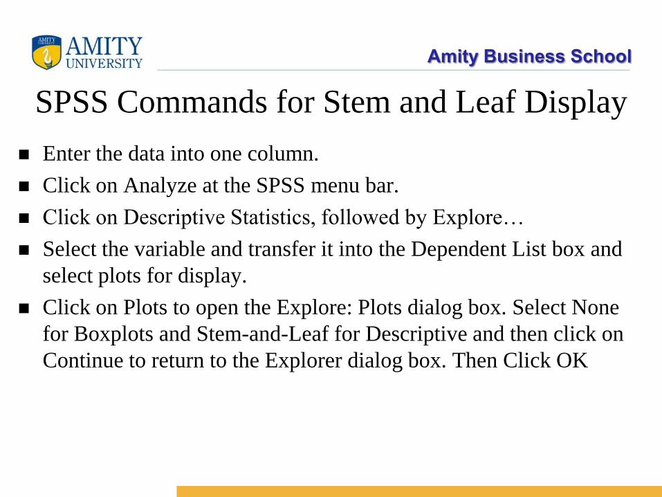
SPSS Commands for Stem and Leaf Display

Enter the data into one column.


Click on Descriptive Statistics, followed by Explore…

Select the variable and transfer it into the Dependent List box and

select plots for display.

Click on Plots to open the Explore: Plots dialog box. Select None

for Boxplots and Stem-and-Leaf for Descriptive and then click on

Continue to return to the Explorer dialog box. Then Click OK


Ogive

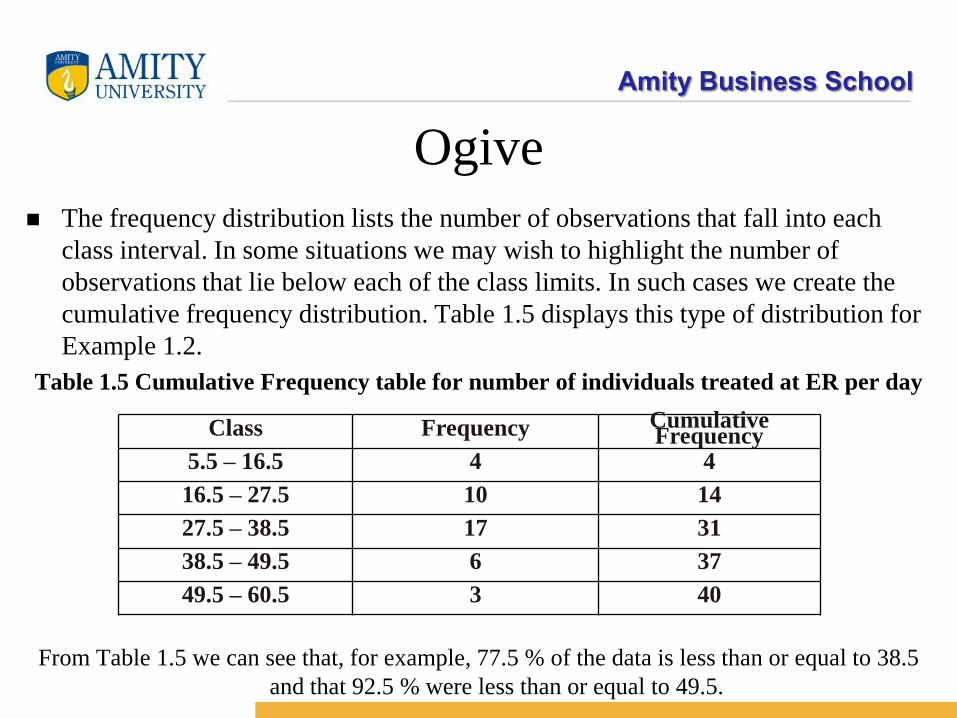
The frequency distribution lists the number of observations that fall into each

class interval. In some situations we may wish to highlight the number of

observations that lie below each of the class limits. In such cases we create the

cumulative frequency distribution. Table 1.5 displays this type of distribution for

Example 1.2.

Table 1.5 Cumulative Frequency table for number of individuals treated at ER per day

From Table 1.5 we can see that, for example, 77.5 % of the data is less than or equal to 38.5

and that 92.5 % were less than or equal to 49.5.

Class Frequency Cumulative Frequency

5.5 – 16.5 4 4

16.5 – 27.5 10 14

27.5 – 38.5 17 31

38.5 – 49.5 6 37

49.5 – 60.5 3 40


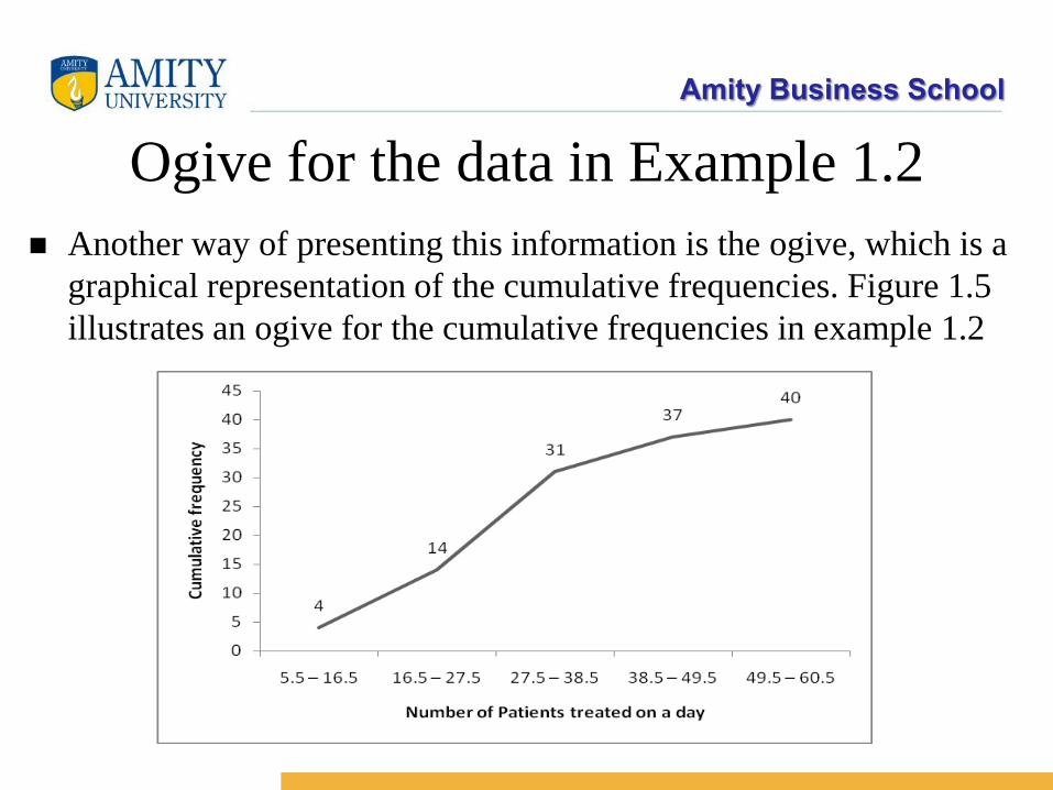
Ogive for the data in Example 1.2

Another way of presenting this information is the ogive, which is a

graphical representation of the cumulative frequencies. Figure 1.5

illustrates an ogive for the cumulative frequencies in example 1.2


Summary

A set of data, even if modest in size, is often difficult to interpret

directly in the form in which it is gathered. Graphical methods

provide procedures for organizing and summarizing data so that

patterns are revealed and the data are more easily interpreted.

Frequency distributions, relative frequency distributions, percent

frequency distributions, bar graphs, and pie charts were presented

as tabular and graphical procedures for summarizing qualitative

data. Frequency distributions, relative frequency distributions,

percent frequency distributions, histograms, cumulative frequency

distributions, and ogives were presented as ways of summarizing

quantitative data. A stem-and-leaf display provides an exploratory

data analysis technique that can be used to summarize quantitative

data.


Self Test

1. A frequency distribution is a tabular summary of data showing the

a. fraction of items in several classes

b. percentage of items in several classes

c. relative percentage of items in several classes

d. number of items in several classes

2. Qualitative data can be graphically represented by using a(n)

a. histogram

b. frequency polygon

c. ogive

d. bar graph


3. The relative frequency of a class is computed by

a. dividing the midpoint of the class by the sample size

b. dividing the frequency of the class by the midpoint

c. dividing the sample size by the frequency of the class

d. dividing the frequency of the class by the sample size

4. The percent frequency of a class is computed by

a. multiplying the relative frequency by 10

b. dividing the relative frequency by 100

c. multiplying the relative frequency by 100

d. adding 100 to the relative frequency


5. Fifteen percent of the students in a school of Business

Administration are majoring in Economics, 20% in Finance, 35% in

Management, and 30% in Accounting. The graphical device(s)

which can be used to present these data is (are)

a. a line graph

b. only a bar graph

c. only a pie chart

d. both a bar graph and a pie chart


6. A cumulative relative frequency distribution shows

a. the proportion of data items with values less than or equal to the

upper limit of each class

b. the proportion of data items with values less than or equal to the

lower limit of each class

c. the percentage of data items with values less than or equal to the

upper limit of each class

d. the percentage of data items with values less than or equal to the

lower limit of each class


7. The most common graphical presentation of quantitative data is a

a. histogram

b. bar graph

c. relative frequency

d. pie chart

8. In constructing a frequency distribution, the approximate class

width is computed as

a. (largest data value - smallest data value)/number of classes

b. (largest data value - smallest data value)/sample size

c. (smallest data value - largest data value)/sample size

d. largest data value/number of classes


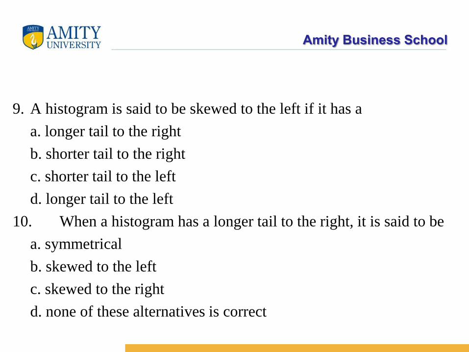
9. A histogram is said to be skewed to the left if it has a

a. longer tail to the right

b. shorter tail to the right

c. shorter tail to the left

d. longer tail to the left

10. When a histogram has a longer tail to the right, it is said to be

a. symmetrical

b. skewed to the left

c. skewed to the right

d. none of these alternatives is correct


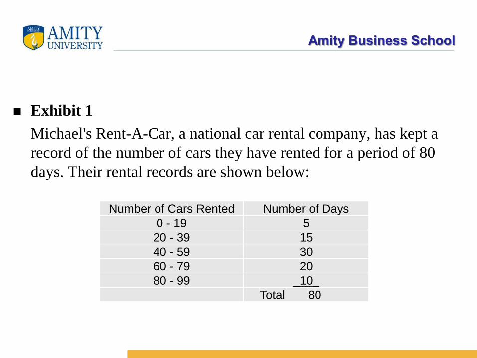
Exhibit 1

Michael's Rent-A-Car, a national car rental company, has kept a

record of the number of cars they have rented for a period of 80

days. Their rental records are shown below:

Number of Cars Rented Number of Days

0 - 19 5

20 - 39 15

40 - 59 30

60 - 79 20

80 - 99 _10_

Total 80


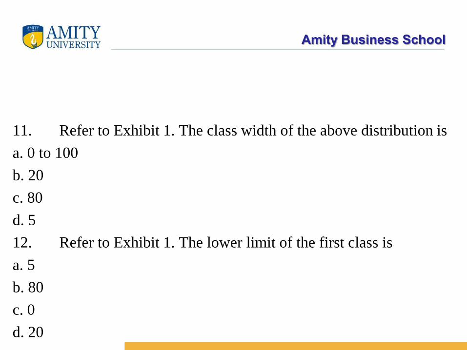
11. Refer to Exhibit 1. The class width of the above distribution is

a. 0 to 100

b. 20

c. 80

d. 5

12. Refer to Exhibit 1. The lower limit of the first class is

a. 5

b. 80

c. 0

d. 20


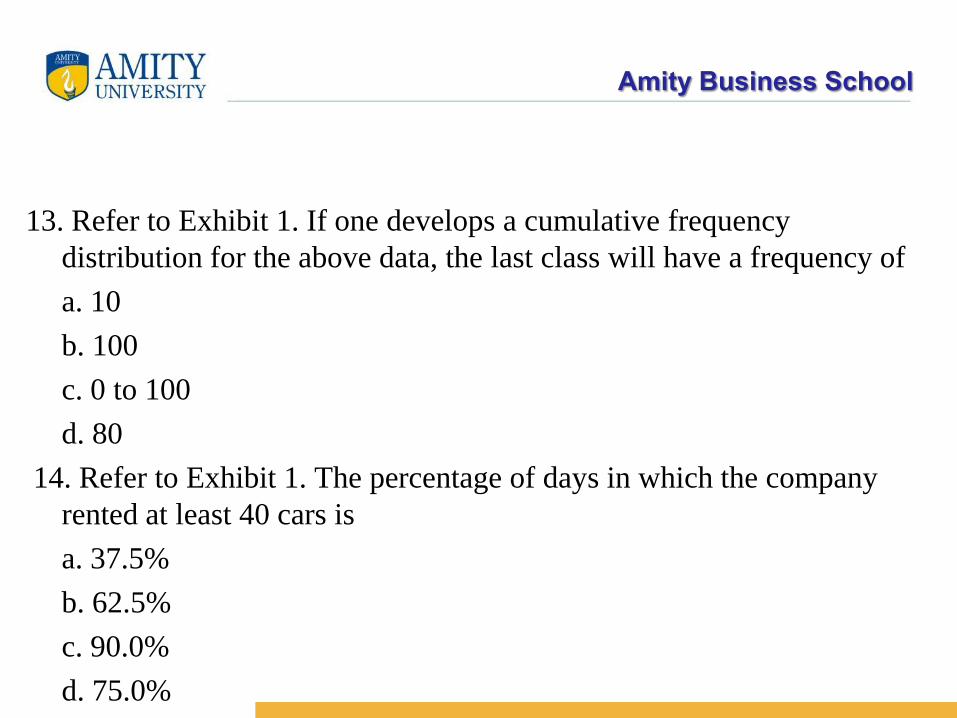
13. Refer to Exhibit 1. If one develops a cumulative frequency

distribution for the above data, the last class will have a frequency of

a. 10

b. 100

c. 0 to 100

d. 80

14. Refer to Exhibit 1. The percentage of days in which the company

rented at least 40 cars is

a. 37.5%

b. 62.5%

c. 90.0%

d. 75.0%


15. Refer to Exhibit 1. The number of days in which the company

rented less than 60 cars is

a. 20

b. 30

c. 50

d. 60


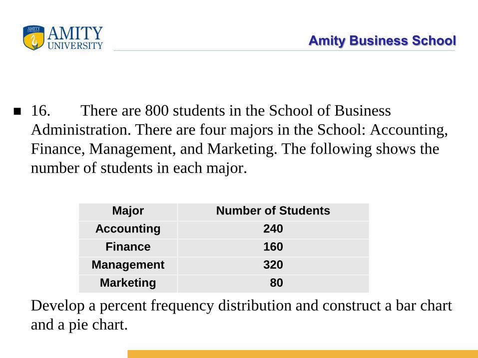
16. There are 800 students in the School of Business

Administration. There are four majors in the School: Accounting,

Finance, Management, and Marketing. The following shows the

number of students in each major.

Develop a percent frequency distribution and construct a bar chart

and a pie chart.

Major Number of Students

Accounting 240

Finance 160

Management 320

Marketing 80


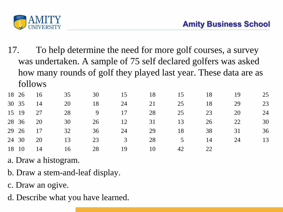
17. To help determine the need for more golf courses, a survey

was undertaken. A sample of 75 self declared golfers was asked

how many rounds of golf they played last year. These data are as

follows18 26 16 35 30 15 18 15 18 19 25

30 35 14 20 18 24 21 25 18 29 23

15 19 27 28 9 17 28 25 23 20 24

28 36 20 30 26 12 31 13 26 22 30

29 26 17 32 36 24 29 18 38 31 36

24 30 20 13 23 3 28 5 14 24 13

18 10 14 16 28 19 10 42 22

a. Draw a histogram.

b. Draw a stem-and-leaf display.

c. Draw an ogive.

d. Describe what you have learned.

Documents

Diagrammatic &Graphical Presentation of Data