Diagram 70. The Integer-Array Arr - … advanced/Data Struct Adv 2012... · Flowchart of Selection Sort Do this as an exercise. ... Pseudocode of Bubble Sort The following pseudocode

Intro to Data Structures and HLL Prog 5: Searching and Sorting (eac) Page 1

6. Standard Algorithms

The algorithms we will examine perform Searching and Sorting. 6.1 Searching Algorithms

Two algorithms will be studied. These are:

The Linear Search

The Binary Search

6.1.1. Linear Search

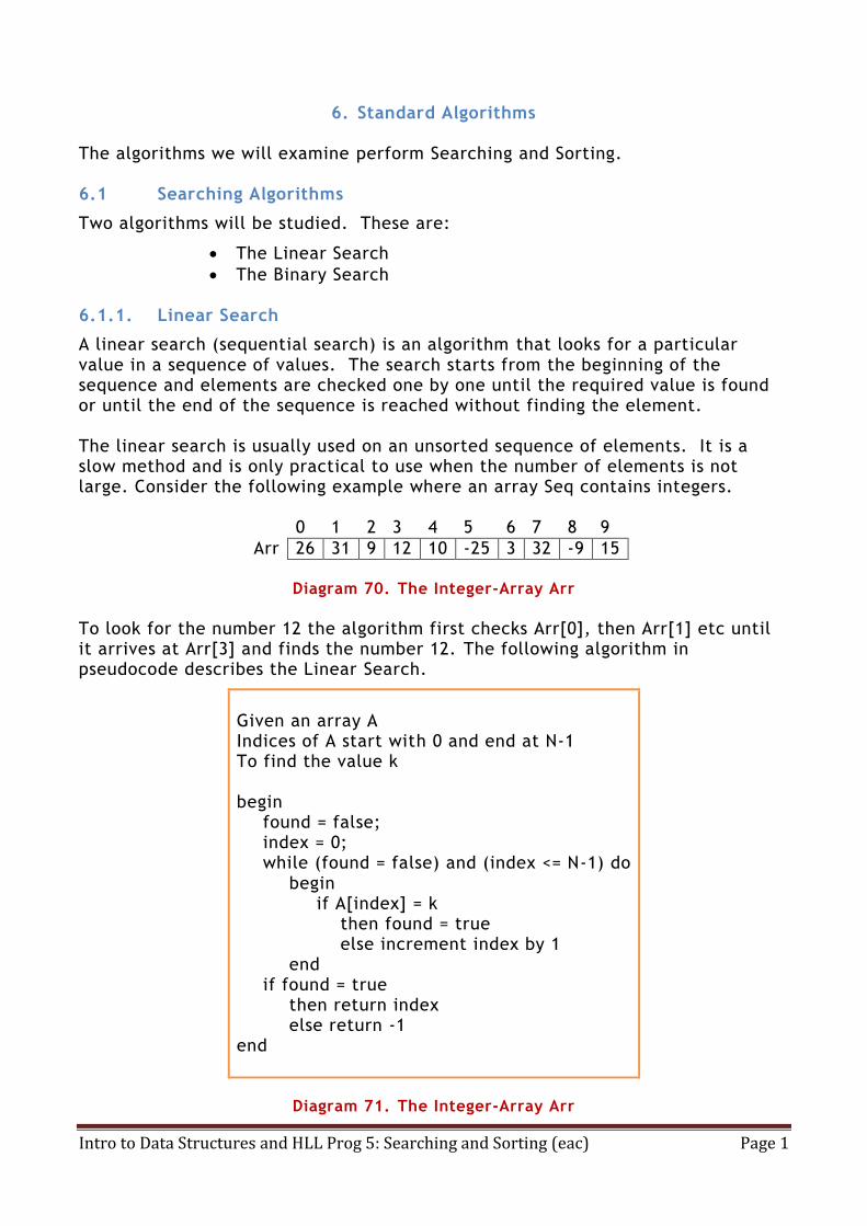
A linear search (sequential search) is an algorithm that looks for a particular value in a sequence of values. The search starts from the beginning of the sequence and elements are checked one by one until the required value is found or until the end of the sequence is reached without finding the element. The linear search is usually used on an unsorted sequence of elements. It is a slow method and is only practical to use when the number of elements is not large. Consider the following example where an array Seq contains integers.

0 1 2 3 4 5 6 7 8 9

Arr 26 31 9 12 10 -25 3 32 -9 15

Diagram 70. The Integer-Array Arr

To look for the number 12 the algorithm first checks Arr[0], then Arr[1] etc until it arrives at Arr[3] and finds the number 12. The following algorithm in pseudocode describes the Linear Search.

Given an array A Indices of A start with 0 and end at N-1 To find the value k begin found = false; index = 0; while (found = false) and (index <= N-1) do begin if A[index] = k then found = true else increment index by 1 end if found = true then return index else return -1 end

Diagram 71. The Integer-Array Arr


6.1.1.1. Exercise on Linear Search

Draw a flowchart of the Linear Search. 6.1.2. Binary Search

The binary search is a very fast search on a sequence of SORTED elements. The reasoning behind this kind of search is to look at the element in the middle and if it is not the element required then the range of elements to be searched is halved. Let us consider an example. In the array A below let us search for the element 34 by following the binary search algorithm.

0 1 2 3 4 5 6 7 8 9 10 11 12 13 14

5 12 19 25 29 34 38 45 46 50 57 64 70 77 85

Diagram 72. A Sorted Array

First = 0; Last = 14; Mid = int ( (First + Last)/2 ) = 7 Check if A[7] = 34 or not. Since A[7] is not equal to 34 then it is not yet found. However, since the elements are sorted, we know that 34, if it is present in the sequence, must be in the region from A[0] to A[6] since A[7] = 45 and 45 > 34. Now correct the values of First, Last and Mid. First = 0; Last = 6; Mid = 3. Is A[3] = 34? No. Therefore adjust First, Last and Mid again. Since A[3] = 25 < 34 then: First = 4; Last = 6; Mid = 5. Is A[5] = 34? Yes. Then the element 34 was found at index 5.

The pseudocode of the binary search is shown hereunder.

BinarySearch (array A; value val) // val is the value to be searched in array A //A has indices that start from 0 and end at N-1 begin first = 0; last = N-1; found = false;


while (first <= last) and (found = false) begin mid = int (first + last)/2 ); if A[mid] = val then begin found = true; pos = mid; end; if A[mid] > val then last = mid – 1; if A[mid] < val then first = mid + 1 end; if found then return pos else return -1 end

Diagram 73. Pseudocode of Binary Search

6.1.2.1. Exercise on Binary Search

a) In the following array manually search for the elements 31, 85 and 25.

0 1 2 3 4 5 6 7 8 9 10 11 12 13

12 18 23 31 36 42 54 55 59 63 70 77 85 92

b) Draw a flowchart of the binary search.

c) Write an algorithm of the binary search using recursion.

6.2 Sorting Algorithms There are many sorting algorithms, some are slow in execution and some are fast. Here we will consider five of these algorithms which are:

Insertion Sort

Selection Sort

Bubble Sort

Quick Sort

Merge Sort 6.2.1. Insertion Sort The Insertion Sort picks elements one by one and each time it sorts the picked elements until all the elements are sorted. Here is an example.


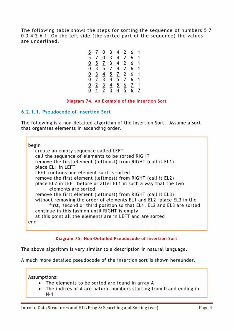
The following table shows the steps for sorting the sequence of numbers 5 7 0 3 4 2 6 1. On the left side (the sorted part of the sequence) the values are underlined.

5 7 0 3 4 2 6 1 5 7 0 3 4 2 6 1 0 5 7 3 4 2 6 1 0 3 5 7 4 2 6 1 0 3 4 5 7 2 6 1 0 2 3 4 5 7 6 1 0 2 3 4 5 6 7 1 0 1 2 3 4 5 6 7

Diagram 74. An Example of the Insertion Sort

6.2.1.1. Pseudocode of Insertion Sort The following is a non-detailed algorithm of the Insertion Sort. Assume a sort that organises elements in ascending order.

begin create an empty sequence called LEFT call the sequence of elements to be sorted RIGHT remove the first element (leftmost) from RIGHT (call it EL1) place EL1 in LEFT LEFT contains one element so it is sorted remove the first element (leftmost) from RIGHT (call it EL2) place EL2 in LEFT before or after EL1 in such a way that the two

elements are sorted remove the first element (leftmost) from RIGHT (call it EL3) without removing the order of elements EL1 and EL2, place EL3 in the

first, second or third position so that EL1, EL2 and EL3 are sorted continue in this fashion until RIGHT is empty at this point all the elements are in LEFT and are sorted end

Diagram 75. Non-Detailed Pseudocode of Insertion Sort

The above algorithm is very similar to a description in natural language. A much more detailed pseudocode of the insertion sort is shown hereunder.

Assumptions:

The elements to be sorted are found in array A

The indices of A are natural numbers starting from 0 and ending in N-1


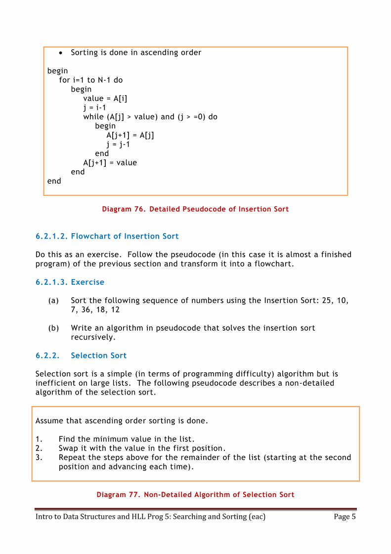
Sorting is done in ascending order begin for i=1 to N-1 do begin value = A[i] j = i-1 while (A[j] > value) and (j > =0) do begin A[j+1] = A[j] j = j-1 end A[j+1] = value end end

Diagram 76. Detailed Pseudocode of Insertion Sort

6.2.1.2. Flowchart of Insertion Sort Do this as an exercise. Follow the pseudocode (in this case it is almost a finished program) of the previous section and transform it into a flowchart. 6.2.1.3. Exercise

(a) Sort the following sequence of numbers using the Insertion Sort: 25, 10,

7, 36, 18, 12 (b) Write an algorithm in pseudocode that solves the insertion sort

recursively.

6.2.2. Selection Sort Selection sort is a simple (in terms of programming difficulty) algorithm but is inefficient on large lists. The following pseudocode describes a non-detailed algorithm of the selection sort.

Assume that ascending order sorting is done. 1. Find the minimum value in the list. 2. Swap it with the value in the first position. 3. Repeat the steps above for the remainder of the list (starting at the second

position and advancing each time).

Diagram 77. Non-Detailed Algorithm of Selection Sort


Effectively, the list is divided into two parts:

The sublist of items already sorted, which is built up from left to right .

The sublist of items remaining to be sorted, occupying the remainder of the sequence.

Here is an example of this sort algorithm sorting five elements:

64 25 12 22 11 11 25 12 22 64 11 12 25 22 64 11 12 22 25 64 11 12 22 25 64

6.2.2.1. Detailed Pseudocode of Selection Sort

Here is a more detailed algorithm of the Selection Sort.

Selection_Sort (Arr, n) // Arr is the name of the array to be sorted // n is the number of elements to be sorted // the indices of the array vary from 0 to n-1 begin index = n-1 while index > 1 do begin greatest = Arr[0] position = 0

counter = 1 while counter < index do begin

if greatest < Arr[counter] then begin

greatest = Arr[counter] position = counter

end counter++

end swap Arr[position] with Arr[index] index –-

end end

Diagram 78. Detailed Algorithm of Selection Sort


6.2.2.2. Flowchart of Selection Sort

Do this as an exercise. Follow the detailed pseudocode.

6.2.2.3. Exercise

(a) Sort the following sequence of numbers using the Selection Sort: 25, 10, 7, 36, 18, 12

(b) Write an algorithm in pseudocode that solves the Selection Sort recursively.

6.2.3. Bubble Sort The Bubble Sort is a simple sorting algorithm. It works by repeatedly going through the list to be sorted and compares each pair of adjacent elements. If the two values are in the wrong order then the elements are swapped. This means that if the algorithm is performing a sort in ascending order and A and B are compared then they are swapped if A>B.

After one “pass” (a “pass” is performed when each pair of adjacent elements is compared) other passes are repeated until the list of elements is sorted. The algorithm gets its name from the way smaller elements "bubble" to the top of the list. As an example let us take the array of numbers "5 1 4 2 8", and sort it in ascending order. In each step the underscored elements are the ones being compared.

First Pass:

( 5 1 4 2 8 ) to ( 1 5 4 2 8 ). Here the algorithm compares the first two elements, and swaps them. ( 1 5 4 2 8 ) to ( 1 4 5 2 8 ). Swap since 5 > 4. ( 1 4 5 2 8 ) to ( 1 4 2 5 8 ). Swap since 5 > 2. ( 1 4 2 5 8 ) to ( 1 4 2 5 8 ). Now, since these elements are already in order (8 > 5) the algorithm does not swap them.

Second Pass:

( 1 4 2 5 8 ) to ( 1 4 2 5 8 ). No swap. ( 1 4 2 5 8 ) to ( 1 2 4 5 8 ). Swap since 4 > 2. ( 1 2 4 5 8 ) to ( 1 2 4 5 8 ). No swap. ( 1 2 4 5 8 ) to ( 1 2 4 5 8 ). No swap Now, the array is already sorted, but our algorithm does not know if it is completed. The algorithm needs one whole pass without any swap to know it is sorted.


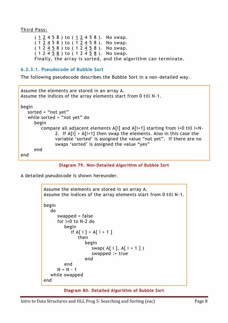
Third Pass:

( 1 2 4 5 8 ) to ( 1 2 4 5 8 ). No swap. ( 1 2 4 5 8 ) to ( 1 2 4 5 8 ). No swap. ( 1 2 4 5 8 ) to ( 1 2 4 5 8 ). No swap. ( 1 2 4 5 8 ) to ( 1 2 4 5 8 ). No swap. Finally, the array is sorted, and the algorithm can terminate.

6.2.3.1. Pseudocode of Bubble Sort

The following pseudocode describes the Bubble Sort in a non-detailed way.

Assume the elements are stored in an array A. Assume the indices of the array elements start from 0 till N-1. begin sorted = “not yet” while sorted = “not yet” do begin compare all adjacent elements A[i] and A[i+1] starting from i=0 till i=N-

2. If A[i] > A[i+1] then swap the elements. Also in this case the variable ‘sorted’ is assigned the value “not yet”. If there are no swaps ‘sorted’ is assigned the value “yes”

end end

Diagram 79. Non-Detailed Algorithm of Bubble Sort

A detailed pseudocode is shown hereunder.

Assume the elements are stored in an array A. Assume the indices of the array elements start from 0 till N-1. begin do swapped = false for i=0 to N-2 do begin if A[ i ] > A[ i + 1 ] then begin swap( A[ i ], A[ i + 1 ] ) swapped := true end end N = N - 1 while swapped end

Diagram 80. Detailed Algorithm of Bubble Sort


6.2.3.2. Flowchart of Bubble Sort Work out the flowchart of the bubble sort as an exercise.

6.2.3.3. Exercise

(a) Perform the bubble sort on the following sequence of numbers: 25, 48, 23, 60, 33

(b) In the detailed pseudocode of the bubble sort we find the statement N = N – 1. Why is this statement present?

(c) Work out a recursive algorithm of the Bubble Sort.

6.2.4. Quick Sort Quicksort is a very efficient sorting algorithm. It works in this way:

1. Choose the “pivot”. This is one of the elements to be sorted.

We choose the leftmost element as the pivot. 2. Find the pivot’s sorted place. When the pivot is placed in its

correct position it leaves two sequences (one on its left and one on its right) to be sorted. The sequence on its left is made up of all the elements smaller than the pivot (assuming sorting in ascending order) while the sequence on its right is made up of all the elements bigger than the pivot.

3. Repeat steps 1 and 2 on the two sequences and repeat recursively.

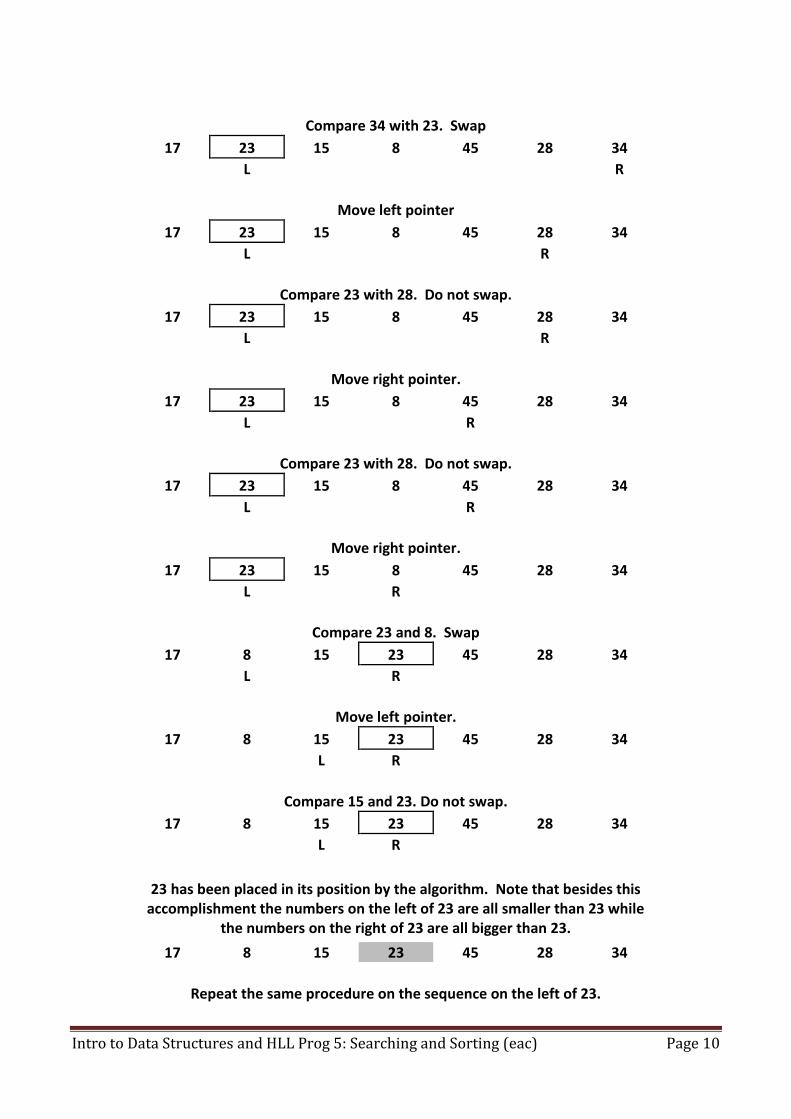
The following example shows the sequence 23, 34, 15, 8, 45, 28 and 17 being sorted in ascending order using the Quicksort.

Sequence to be sorted. 23 34 15 8 45 28 17

Choose 23 as the pivot.

23 34 15 8 45 28 17

Include left (L) and right (R) pointers.

23 34 15 8 45 28 17

L

R

Compare numbers at left and right pointers i.e. compare 23 with 17. Swap.

17 34 15 8 45 28 23

L

R

Move left pointer.

17 34 15 8 45 28 23

L

R


Compare 34 with 23. Swap

17 23 15 8 45 28 34

L

R

Move left pointer

17 23 15 8 45 28 34

L

R

Compare 23 with 28. Do not swap.

17 23 15 8 45 28 34

L

R

Move right pointer.

17 23 15 8 45 28 34

L

R

Compare 23 with 28. Do not swap.

17 23 15 8 45 28 34

L

R

Move right pointer.

17 23 15 8 45 28 34

L

R

Compare 23 and 8. Swap

17 8 15 23 45 28 34

L

R

Move left pointer.

17 8 15 23 45 28 34

L R

Compare 15 and 23. Do not swap.

17 8 15 23 45 28 34

L R

23 has been placed in its position by the algorithm. Note that besides this

accomplishment the numbers on the left of 23 are all smaller than 23 while the numbers on the right of 23 are all bigger than 23.

17 8 15 23 45 28 34

Repeat the same procedure on the sequence on the left of 23.


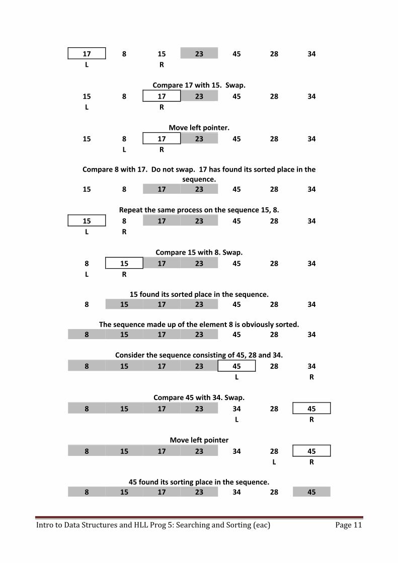
17 8 15 23 45 28 34

L

R

Compare 17 with 15. Swap.

15 8 17 23 45 28 34

L

R

Move left pointer.

15 8 17 23 45 28 34

L R

Compare 8 with 17. Do not swap. 17 has found its sorted place in the

sequence.

15 8 17 23 45 28 34

Repeat the same process on the sequence 15, 8.

15 8 17 23 45 28 34

L R


8 15 17 23 45 28 34

L R

15 found its sorted place in the sequence. 8 15 17 23 45 28 34

The sequence made up of the element 8 is obviously sorted. 8 15 17 23 45 28 34

Consider the sequence consisting of 45, 28 and 34.

8 15 17 23 45 28 34

L

R


8 15 17 23 34 28 45

L

R

Move left pointer

8 15 17 23 34 28 45

L R

45 found its sorting place in the sequence. 8 15 17 23 34 28 45


Consider the sequence 34, 28.

8 15 17 23 34 28 45

L R

Compare 34 and 28. Swap.

8 15 17 23 28 34 45

L R

34 is now in its sorted place.

8 15 17 23 28 34 45

Sequence made up of number 28 is obviously sorted. 8 15 17 23 28 34 45

Diagram 81. An Example of the Quick Sort

The part where the sequence is divided into two is called the “partition phase”. Quicksort makes use of a strategy called “divide and conquer” whereby a task is divided into smaller tasks. Quicksort is also an “in place” algorithm. This means that this algorithm does not use any additional space other than that where the data to be sorted is found. Quicksort is the fastest known sorting algorithm in practice. 6.2.4.1. Pseudocode of Quick Sort

Partition (array, left, right) // assume that the pivot is always the leftmost element begin pivot_value = array[left] pivot_index = left l = left r = right while r > l do begin if array[l] > array[r] then begin //swap array[l] with array[r] temp = array[l] array[l] = array[r] array[r] = temp if pivot_index = l then pivot_index = r


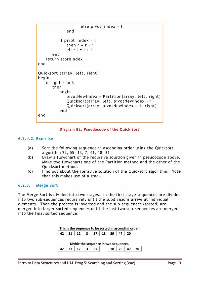
else pivot_index = l end if pivot_index = l then r = r – 1 else l = l + 1 end return storeIndex end Quicksort (array, left, right) begin if right > left then begin pivotNewIndex = Partition(array, left, right) Quicksort(array, left, pivotNewIndex - 1) Quicksort(array, pivotNewIndex + 1, right) end end

Diagram 82. Pseudocode of the Quick Sort

6.2.4.2. Exercise

(a) Sort the following sequence in ascending order using the Quicksort

algorithm 22, 55, 13, 7, 41, 18, 31 (b) Draw a flowchart of the recursive solution given in pseudocode above.

Make two flowcharts one of the Partition method and the other of the Quicksort method.

(c) Find out about the iterative solution of the Quicksort algorithm. Note that this makes use of a stack.

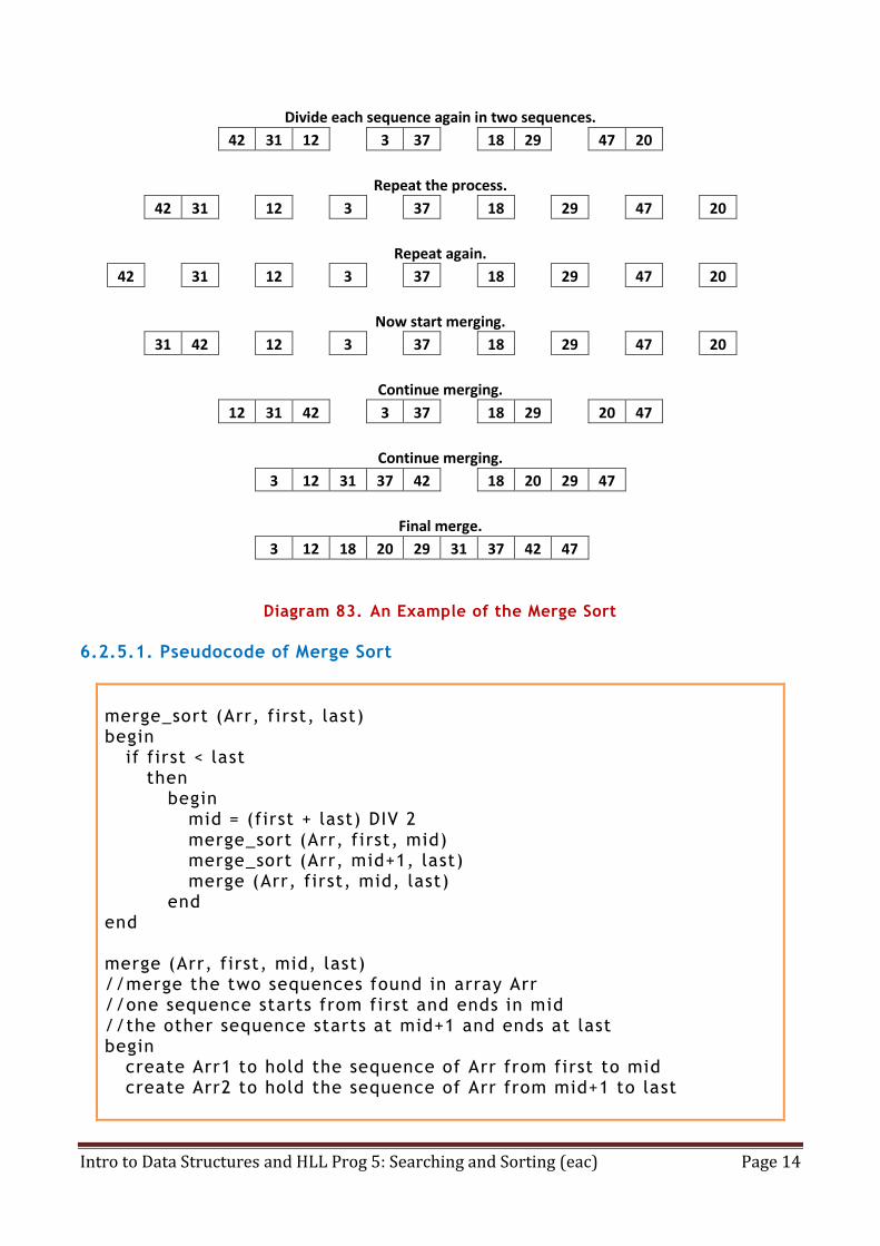
6.2.5. Merge Sort The Merge Sort is divided into two stages. In the first stage sequences are divided into two sub-sequences recursively until the subdivisions arrive at individual elements. Then the process is inverted and the sub-sequences (sorted) are merged into larger sorted sequences until the last two sub-sequences are merged into the final sorted sequence.

This is the sequence to be sorted in ascending order.

42 31 12 3 37 18 29 47 20

Divide the sequence in two sequences.

42 31 12 3 37

18 29 47 20


Divide each sequence again in two sequences.

42 31 12

3 37

18 29

47 20

Repeat the process.

42 31

12

3

37

18

29

47

20

Repeat again.

42

31

12

3

37

18

29

47

20

Now start merging.

31 42

12

3

37

18

29

47

20

Continue merging.

12 31 42

3 37

18 29

20 47

Continue merging.

3 12 31 37 42

18 20 29 47

Final merge.

3 12 18 20 29 31 37 42 47

Diagram 83. An Example of the Merge Sort

6.2.5.1. Pseudocode of Merge Sort

merge_sort (Arr, first, last) begin if first < last then begin mid = (first + last) DIV 2 merge_sort (Arr, first, mid) merge_sort (Arr, mid+1, last) merge (Arr, first, mid, last) end end merge (Arr, first, mid, last) //merge the two sequences found in array Arr //one sequence starts from first and ends in mid //the other sequence starts at mid+1 and ends at last begin create Arr1 to hold the sequence of Arr from first to mid create Arr2 to hold the sequence of Arr from mid+1 to last


copy the elements from first to mid from array Arr to array [Arr1 copy the elements from mid+1 to last from array Arr to array [Arr2 //merge the two sequences set two pointers p_Arr1 and p_Arr2 at the start of eachsequence set another pointer p_Arr at the start of Arr while there are still elements in both Arr1 and Arr2 that have [not been copied to Arr do begin if Arr1[p_Arr1] < Arr2[p_Arr2] then begin place Arr1[p_Arr1] in Arr at p_Arr increment p_Arr by 1 increment p_Arr1 by 1 end else begin place Arr2[p_Arr2] in Arr at p_Arr increment p_Arr by 1 increment p_Arr2 by 1 end end place remaining (sorted) elements in Arr1 or Arr2 in A rr end

Diagram 84. Pseudocode of the Merge Sort

6.2.5.2. Exercise

a) Sort the following sequence using the Merge Sort: 34, 78, 17, 55, 3, 61, 12. b) Draw the flowchart of the Merge Sort (from the above pseudocode). c) Find out about the iterative solution.

6.2.6. Big-O Notation

Big O notation is used in Computer Science to describe the performance (complexity) of an algorithm. Big O can be used to describe the execution time required or the space used (memory) by an algorithm. O(1)

O(1) describes an algorithm that will always e xecute in the same time (or space) regardless of the size of the input data set. An example of s uch an algorithm is found below.


method IsFirstElementT ( S : string )

begin if ( S[0] = T ) then return true else return false end

Diagram 85. An Algorithm of Complexity O(1)

O(N) O(N) describes an algorithm whose performance will grow linearly and in direct proportion to the size of the input data set. The example below also demonstrates how Big O favours the worst -case performance scenario; a matching string could be found during any iteration of the for loop and the function would return early, but Big O notation will always assume the upper limit where the algorithm will perform the maximum number of iterations.

method ContainsChar ( str, charstr: string )

begin for i = 0 to length (str) -1 do begin if ( str[i] = charstr ) then return true end return false end

Diagram 86. An Algorithm of Complexity O(N)

O(N2)

O(N2) represents an algorithm whose performance is directly proportional to the square of the size of the input data set. This is common with algorithms that involve nested iterations over the data set. Deeper nested iterations will result in O(N 3), O(N4) etc.

bool ContainsDuplicates(String[] strings) { for(int i = 0; i < strings.Length; i++) { for(int j = 0; j < strings.Length; j++) {


if(i == j) // Don't compare with self { continue; } if(strings[i] == strings[j]) { return true; } } } return false; }

Diagram 87. An Algorithm of Complexity O(n2)

O(2N) O(2N) denotes an algorithm whose growth will double with each additional element in the input data set. The execution time of an O(2N) function will quickly become very large.

Logarithms Logarithms are slightly trickier to explain so I’ll use a common example: the binary search technique as you know halves the data set with each iteration until the value is found or until it is found out that the value required is not in the sequence. This type of algorithm is described as O(log N). The iterative halving of data sets described in the binary search example produces a growth curve that peaks at the beginning and slowly flattens out as the size of the data sets increase e.g. an input data set containing 10 items takes one second to complete, a data set containing 100 items takes two seconds, and a data set containing 1000 items will take three seconds. Doubling the size of the input data set has little effect on its growth as after a single iteration of the algorithm the data set will be halved and therefore on a par with an input data set half the size. This makes algorithms like binary search extremely efficient when dealing with large data sets. The following table shows the order of the time of execution and memory in terms of the big-O notation.

Name Best Average Worst Memory

Insertion Sort O(n) O(n2) O(n2) 1


Selection Sort O(n2) O(n2) O(n2) 1

Bubble Sort O(n) O(n2) O(n2) 1

Quick Sort O(n log n) O(n log n) O(n2) O(log n)

Merge Sort O(n log n) O(n log n) O(n log n) n

In-place Merge Sort O(n log n) O(n log n) O(n log n) 1

Diagram 88. Time Complexities of the Sorting Algorithms

Although the Insertion, Selection and Bubble sorts have all the same complexity i.e. their time of execution depends on n2, empirical timings show that the Insertion sort is faster than the Selection sort which is then faster than the Bubble sort. The same comparison can be done with the Quick sort and the Merge sort. The Quick sort is faster than the Merge sort in the average case.

Documents

Diagram 70. The Integer-Array Arr - … advanced/Data Struct Adv 2012... · Flowchart of Selection Sort Do this as an exercise. ... Pseudocode of Bubble Sort The following pseudocode