Diagnostic Pressure Equation as a Weak Constraint in a

Diagnostic Pressure Equation as a Weak Constraint in a Storm-ScaleThree-Dimensional Variational Radar Data Assimilation System

GUOQING GE

Center for Analysis and Prediction of Storms, University of Oklahoma, Norman, Oklahoma

JIDONG GAO

NOAA/National Severe Storm Laboratory, Norman, Oklahoma

MING XUE

Center for Analysis and Prediction of Storms, and School of Meteorology, University of Oklahoma,

Norman, Oklahoma

(Manuscript received 16 November 2011, in final form 20 March 2012)

ABSTRACT

A diagnostic pressure equation is incorporated into a storm-scale three-dimensional variational data as-

similation (3DVAR) system in the form of a weak constraint in addition to a mass continuity equation

constraint (MCEC). The goal of this diagnostic pressure equation constraint (DPEC) is to couple different

model variables to help build a more dynamic consistent analysis, and therefore improve the data assimilation

results and subsequent forecasts. Observational System Simulation Experiments (OSSEs) are first performed

to examine the impact of the pressure equation constraint on storm-scale radar data assimilation using an

idealized tornadic thunderstorm simulation. The impact of MCEC is also investigated relative to that of

DPEC. It is shown that DPEC can improve the data assimilation results slightly after a given period of data

assimilation. Including both DPEC and MCEC yields the best data assimilation results. Sensitivity tests show

that MCEC is not very sensitive to the choice of its weighting coefficients in the cost function, while DPEC is

more sensitive and its weight should be carefully chosen. The updated 3DVAR system with DPEC is further

applied to the 5 May 2007 Greensburg, Kansas, tornadic supercell storm case assimilating real radar data. It

is shown that the use of DPEC can speed up the spinup of precipitation during the intermittent data assim-

ilation process and also improve the follow-on forecast in terms of the general evolution of storm cells and

mesocyclone rotation near the time of observed tornado.

1. Introduction

There are many challenges in forecasting convective

storms. One of them is how to produce a dynamic con-

sistent initial condition for storm-scale numerical weather

prediction (NWP) (see the appendix for acronym ex-

pansions and variable definitions) models. Currently, the

Weather Surveillance Radar-1988 Doppler (WSR-88D)

network is the only source of routine observations in the

United States that can resolve storm-scale features at

high enough spatial and temporal resolutions. Therefore,

in recent years, many studies are focused on the assim-

ilation of these radar data into NWP models to provide

better initial conditions (e.g., Crook and Tuttle 1994;

Sun and Crook 1997; Sun and Crook 2001; Hu et al.

2006a,b; Stensrud and Gao 2010). The problem is chal-

lenging because the radar only observes a few parameters,

typically limited to the radial velocity and reflectivity,

while most state variables have to be ‘‘retrieved’’ in the

data assimilation (DA) process.

Several DA methods have been applied to the radar

DA problem; they include three-dimensional variational

data assimilation (3DVAR), four-dimensional variational

data assimilation (4DVAR), and ensemble Kalman fil-

ter (EnKF). The 4DVAR method is attractive because it

Corresponding author address: Dr. Jidong Gao, 120 David L.

Boren Blvd., National Severe Storm Laboratory, Norman, OK

73072.

E-mail: [email protected]

AUGUST 2012 G E E T A L . 1075

DOI: 10.1175/JTECH-D-11-00201.1

� 2012 American Meteorological Society

uses an NWP model as a strong constraint and tries to fit

the model state to observations taken at different times

during the assimilation window, thereby producing a dy-

namically consistent state and retrieving unobserved

variables. Sun and Crook (1997, 1998) and Sun (2005)

had shown encouraging results with a 4DVAR based on

a cloud model. However, the need to develop and

maintain complex adjoint codes for NWP models and

the difficulties encountered with complex ice micro-

physics that are important for storm-scale predictions

have limited the adoption of the 4DVAR method in

storm-scale NWP operations. The EnKF is an emerging

technique, which promises to produce similar assimila-

tion quality as 4DVAR, but avoids the coding of an

adjoint model. Many radar DA studies have been car-

ried out in recent years with EnKF (e.g., Snyder and

Zhang 2003; Zhang et al. 2004; Caya et al. 2005; Tong

and Xue 2005; Xue et al. 2006; Aksoy et al. 2009; Zhang

et al. 2009; Aksoy et al. 2010; Dowell et al. 2011; Snook

et al. 2011). These studies have shown the great poten-

tial of the EnKF method. On the other hand, EnKF

is not as mature as the variational methods and so far

successful applications to real data assimilation prob-

lems are still limited. Computationally, it has similar

costs to 4DVAR.

The 3DVAR method is computationally much more

efficient, making its real-time applications much more

practical. Some studies (e.g., Hu et al. 2006a,b; Hu and

Xue 2007a; Stensrud and Gao 2010) have successfully

demonstrated the ability of the 3DVAR to assimilate

radar data to predict tornadic supercell storms. The

Advanced Regional Prediction System (ARPS; Xue

et al. 2000, 2001, 2003) 3DVAR system and its cloud

analysis package have been used to produce continental

U.S.–scale real-time weather predictions at up to 1-km

resolution (Xue et al. 2008, 2011). However, despite its

successful applications, the 3DVAR method is often

challenged by its theoretical suboptimality resulting from

its use of static background error covariance and the lack

of suitable balances among model variables. Research

efforts have been made to incorporate flow-dependent

background error covariance in a 3DVAR framework.

For example, Liu and Xue (2006) and Liu et al. (2007)

reported efforts to build flow-dependent background

error covariance in a 3DVAR system using anisotropic

recursive filters and demonstrated improvement in mois-

ture retrieval from GPS slant-path water vapor observa-

tions. Hamill and Snyder (2000), Lorenc (2003), Buehner

(2005), and Wang et al. (2008a,b) advocated a hybrid

approach that incorporates flow-dependent background

covariance derived from an forecast ensemble into

a 3DVAR framework, and the method is recently ap-

plied to a radar DA problem for a landfalling hurricane

(Li et al. 2012). The similar methodology can be ex-

tended to 4DVAR also. Because of the use of an en-

semble, the method is also expensive and requires much

research.

Another alternative to improve the balance among

model variables in the 3DVAR analysis is to include

suitable weak constraints in the 3DVAR cost function,

which also helps spread observational information to

state variables not directly observed. Gao et al. (1999,

2001, 2004), Hu et al. (2006a,b) and Hu and Xue (2007b)

incorporated an anelastic mass continuity equation into

the cost function of the ARPS 3DVAR system as a weak

constraint and found that this constraint can improve the

wind analysis and subsequent storm forecasts. However,

there is no direct linkage between the wind and ther-

modynamic (pressure and temperature) variables in the

system. Xiao et al. (2005) reported their efforts to build

linkages between the wind and thermodynamic fields in

the Fifth-Generation NCAR/Penn State Mesoscale Mode)

MM5 3DVAR system by using a constraint based on

a linearized Richardson equation, which is derived from

mass continuity, adiabatic thermodynamic, and hydro-

static equations. The hydrostatic and adiabatic assump-

tions in their study are not suitable for the storm-scale

DA, however. Some other 3DVAR radar analysis and

assimilation studies (e.g., Protat and Zawadzki 2000; Liou

2001; Protat et al. 2001; Weygandt et al. 2002a,b; Liou

et al. 2003; Zhao et al. 2006, 2008; Liou and Chang 2009)

turned to a two-step approach, where a thermodynamic

retrieval technique is applied to derive the temperature

and pressure fields from several time levels of retrieved

wind fields. This technique was pioneered by Gal-Chen

(1978) and Hane and Scott (1978). One of the difficulties

with such an approach lies with the accurate retrieval of

three wind components and their time tendencies, which

by itself is a difficult problem. The results are especially

sensitive to the estimate of the time tendencies (Crook

1994).

In the equation constraint to be introduced in this

study, the calculation of the wind tendency term is avoi-

ded by applying the divergence operator to the three

model momentum equations. The derived equation is the

diagnostic pressure equation in typical anelastic systems

where three momentum tendency terms cancel out. This

diagnostic pressure equation is incorporated into our

3DVAR cost function in the form of a weak constraint in

addition to the aforementioned mass continuity equa-

tion constraint (MCEC). The main goal of this constraint

is to improve the consistency between dynamic and

thermodynamic fields. Xu et al. (2001) tried to include

a similar constraint in their simple adjoint system for re-

trieving three-dimensional winds from single-Doppler

radar that treats the radial velocity as a tracer. They found

1076 J O U R N A L O F A T M O S P H E R I C A N D O C E A N I C T E C H N O L O G Y VOLUME 29

that the DPEC can help improve the retrieval of wind

fields in single time data analysis. However, the impact

of DPEC through intermittent data assimilation cycles,

and on the follow-on forecasts, has not been investigated

in a full NWP model.

In this paper, we will discuss the development of the

DPEC within the ARPS 3DVAR framework and its

tests with supercell thunderstorms. The rest of the paper

is organized as follows. Section 2 will discuss the schemes

adopted by the 3DVAR system and focus on the de-

velopment and implementation of the DPEC. Section 3

examines the impact of the DPEC on storm analysis and

prediction in an OSSE framework, while section 4 applies

the system to the 5 May 2007 Greensburg, Kansas, tor-

nadic supercell thunderstorm case and examines the im-

pact of the equation constraints on the storm forecast. The

summary and future plan will be presented in section 5.

2. The equation constraints in the ARPS 3DVARsystem

A 3DVAR system within the ARPS model frame-

work (Xue et al. 2000, 2001, 2003) has been developed

and applied to the assimilation of weather radar and

other data (Gao et al. 1999, 2004; Hu et al. 2006a,b; Hu

and Xue 2007b; Xue et al. 2008; Stensrud and Gao 2010).

In the system, the cost function J is written as the sum of

the background and observational terms plus a penalty

or equation constraint term (Jc),

J(x) 5 Jb 1 Jo 1 Jc

51

2(x 2 xb)TB21(x 2 xb)

11

2[H(x)2yo]TR21[H(x) 2 yo] 1 Jc. (1)

Following the standard notion of Ide et al. (1997),

x and xb are the analysis and background state vectors,

and yo is the observation vector. Respectively, B and R

are the background and observation error covariance

matrices, and H(x) is the nonlinear observation opera-

tor. To improve the conditioning of the J minimization

problem and avoid the need for the inverse of B, a new

control variable v is introduced, which is related to the

analysis increment dx 5 x 2 xb according to

dx 5 B1/2v. (2)

In terms of v, the background term becomes,

Jb 5 (1/2)vTv. (3)

Consequently, the minimization is performed in the

space of v. The recursive filter proposed by Purser et al.

(2003a,b) is used to model the effect of the background

error covariance, or more precisely the square root of B.

Currently in our 3DVAR system, the background term xb

can be provided by a sounding profile, the previous ARPS

model forecast, or the forecast from another model. The

analysis vector x contains the three wind components (u, y,

and w), potential temperature (u), pressure ( p), and water

vapor mixing ratio (qv). The observations include Doppler

radar radial velocity, and single- (such as surface ob-

servations) and multiple-level conventional observa-

tions (such as those of rawinsondes and wind profilers).

Term Jc in Eq. (1) includes any penalty or equation

constraint terms. Currently, it includes two terms as

defined in the following:

Jc 5 Q(x)TA21Q Q(x) 1 P(x)TA21

P P(x). (4)

The first term on right-hand side (rhs) of Eq. (4) is

intended to minimize the 3D anelastic mass divergence

so as to provide the key coupling among the three wind

components. The definition and impact of this constraint

have been investigated by Gao et al. (1999, 2004) and Hu

et al. (2006b). In this study, we will reinvestigate its

relative impact and sensitivity to weights as compared to

that of DPEC using OSSE experiments.

The second term on the rhs of Eq. (4) is the DPEC

term in which

P [ $ � E

[ 2 =2p9 2 $ � (rV � $V)

1 g›

›z

"r

u9

u2

p9

rc2s

1q9v

« 1 qv

2q9v 1 qliquid1ice

1 1 qv

!#

1 $ � C 1 $ �D, (5)

where

E 5›(rV)

›t5 i

›(ru)

›t1 j

›(rv)

›t1 k

›(rw)

›t, (6)

V 5 iu 1 jv 1 kw, (7)

C 5 i(rfv 2 r ~f w) 1 j(rfu) 1 k(r ~f u), (8)

D 5 iDu 1 jDy

1 kDw. (9)

The vector E is the forcing term of the vector Euclidian

momentum equations. The primed variables are pertur-

bations from a base state, cs is the acoustic wave speed,

and « is the ratio of the gas constants for dry air and

water vapor. The Coriolis coefficients f 5 2V sin(f) and~f 5 2V cos(f), where V is the angular velocity of the earth

and f is latitude. The terms Du, Dy, and Dw contain the


subgrid-scale turbulence and computational mixing terms.

Other symbols follow conventions and are detailed in the

appendix. When the mass continuity equation is applied,

Eq. (5) becomes P 5 0, where P represents the rhs of (5).

Equation (5) is derived by applying the divergence

operator to the three momentum equations of the ARPS

model (Xue et al. 2000):

r›u

›t5 2rV � $u 2

›p9

›x1 rf y 2 r~f w� �

1 Du, (10)

r›y

›t5 2rV � $y 2

›p9

›y2 rfu 1 D

y, (11)

r›w

›t5 2rV � $w 2

›p9

›z

1 rg

"u9

u2

p9

rc2s

1q9v

« 1 qv

2q9v 1 qliquid1ice

1 1 qv

#

1 r ~f u 1 Dw. (12)

Equations (10)–(12) are the basis of the thermody-

namic retrieval technique mentioned in the previous

section. To obtain a good storm-scale thermodynamic

retrieval, it is required to have a very good estimation of

the three velocity tendency terms on the left-hand side

of Eqs. (10)–(12), that is, r(›u/›t), r(›y/›t), r(›w/›t).

However, this task is often very difficult because the

storm-scale features change very rapidly in time while

radar observations are usually taken every 5–6 min, as is

the case with the U.S. operational WSR-88D radars. The

inaccuracy and incompleteness of the wind observations

from radars worsens the scenario. To overcome this prob-

lem and help establish better balance among model

variables, we incorporate the diagnostic divergence Eq.

(5) into the 3DVAR system in the form of a weak con-

straint [named P in Eq. (4)]. In this way, the calculation

of wind tendency terms is avoided.

The two As in Eq. (4) are the error covariance matrices

associated with the corresponding constraints, which are

assumed to be diagonal with empirically defined constant

diagonal elements as the variances. The inverse diagonal

matrices are called weighting coefficients and determine

the relative importance of each constraint, and their op-

timal values can be determined through numerical ex-

periments, similar to the way to determine certain weights

in cloud-scale variation data assimilation systems (e.g.,

Sun and Crook 2001). Usually, the constraint terms with

their weights should be similar orders of magnitude as

other terms in J for them to be effective.

It is very important to make sure the gradient of the

cost function is computed correctly; otherwise, the mini-

mization is erroneous. Similar to Wang (1993) and Sun

et al. (1991), let x be the analysis vector and J(x) be the

cost function. To expand J(x 1 a$xJ) at the direction $xJ

using the Taylor series, it can be derived that

F(a) 5J(x 1 a$xJ) 2 J(x)

a$xJ � $xJ5 1:0 1 O(ak$xJk). (13)

For a very small a, if the gradient is computed cor-

rectly, then the F(a) should take the value of one. The

FIG. 1. The verification of the gradient calculation variation of (a) f(a)with log(a) and (b)

logjf(a) 2 1j with log(a).

TABLE 1. List of OSSE data assimilation experiments

(see text for details).

DP weighting

coefficient if

used

MC weighting

coefficient if

used

CNTL 4.0 3 106 4.0 3 106

DP 4.0 3 106

MC 4.0 3 106

NoEC

CNTLDd5 8.0 3 105 4.0 3 106

CNTLDm5 2.0 3 107 4.0 3 106

CNTLDd25 1.6 3 105 4.0 3 106

CNTLDm25 1.0 3 108 4.0 3 106

CNTLMd5 4.0 3 106 8.0 3 105

CNTLMm5 4.0 3 106 2.0 3 107

CNTLMd25 4.0 3 106 1.6 3 105

CNTLMm25 4.0 3 106 1.0 3 108


updated ARPS 3DVAR with DPEC has been verified

using the above method. Figure 1 shows that when a

takes a small value from 1025 to 10215, F(a) takes the

value of one up to the computer precision. This justifies

that the gradient calculation is correct.

To check whether the minimization process goes well

after including additional DPEC in the 3DVAR system,

the behavior of the cost function and its individual terms

are examined by plotting the evolution of the cost function

with the number of iterations as similar to Gao et al.

(2001). It was verified (not shown here) that the total cost

function and the three individual terms (radar observa-

tion, DPEC, and MCEC, respectively) all decrease well in

the minimization process for different cases and different

weighting coefficients. The above tests confirm that the

updated ARPS 3DVAR system with one more weak

constraint (DPEC) works correctly and is ready for the

following idealized testing and real case studies.

FIG. 2. The RMS errors of model fields during the 1-h assimilation period for the (a) u

component of wind, (b) vertical velocity w, (c) perturbation potential temperature, (d)

pressure, (e) water vapor mixing ratio, (f) cloud water mixing ratio, (g) cloud ice mixing ratio,

and (h) simulated reflectivity from model rain/snow/hail mixing ratios. CNTL (purple solid

line), DP (blue dot-dashed line), MC (green dotted line), and NoEC (red solid line) are

shown.


3. The impact of the diagnostic pressure equationconstraint in OSSEs

a. The prediction model and OSSE design

To examine the impact of DPEC on radar data as-

similation in the storm-scale 3DVAR, a series of OSSEs

are conducted using simulated radar data for the 20 May

1977 Del City, Oklahoma, supercell storm (Ray et al.

1981). The ARPS model is used to create a truth simu-

lation of the Del City supercell using a 54 km 3 54 km 3

16 km physical domain with 57 3 57 3 35 grid points and

1-km horizontal and 0.5-km vertical resolutions, re-

spectively. The truth simulation is initialized from a mod-

ified real sounding, as documented in Xue et al. (2001), in

addition to a 14-K ellipsoidal thermal bubble centered

at x 5 48, y 5 16, and z 5 1.5 km, with radii of 10 km in

the x and y directions and 1.5 km in the z direction. The

Lin et al. (1983) three-ice microphysical scheme is used

together with a 1.5-order turbulent kinetic energy sub-

grid parameterization. Open conditions are used at the

lateral boundaries. A wave radiation condition is also

applied at the top boundary. Free-slip conditions are

applied to the bottom boundary. The length of simula-

tion is up to 2 h. A constant wind of u 5 3 m s21 and y 5

14 m s21 is subtracted from the observed sounding to

keep the primary storm cell near the center of model

grid. The evolution of the simulated storms is similar to

those documented in Xue et al. (2001).

In the truth simulation, the supercell rapidly develops

over the first 20 min from the thermal bubble. The strength

of the cell decreases thereafter. At around 55 min, the cell

splits into two. The north-northeastward-moving cell (the

right mover) in the model tends to dominate the system.

Another cell (the left mover) moves northwestward and

splits again at 95 min.

The experiments assimilate simulated radial velocity

(Vr) observations from two radars, which are located at

the southwest (x 5 0 km, y 5 0 km) and southeast (x 5

54 km, y 5 0 km) corners of the model domain. The Vr

observations are assumed to be available at the grid

points and calculated as follows:

Vr 5 u sinc cosl 1y cosc cosl 1w sinl, (14)

where c is the elevation angle; l is the azimuth angle;

and u, y, and w are the three wind components from the

truth simulation. For simplicity, the beam broadening,

earth curvature effects, and the precipitation terminal

velocity are not considered in either observation simula-

tion or assimilation. Random Gaussian noise with a zero

mean and a standard deviation of 1 m s21 is added to the

simulated Vr observations.

The first 3DVAR analysis assimilates radar data taken

from truth simulation at t 5 30 min of model time and its

first guess is horizontally homogeneous, with vertical

variation specified by the same sounding profile as the

truth simulation, which means there is no storm in the

background at this time. From the first analysis, the ARPS

model is run for 5 min when another 3DVAR analysis

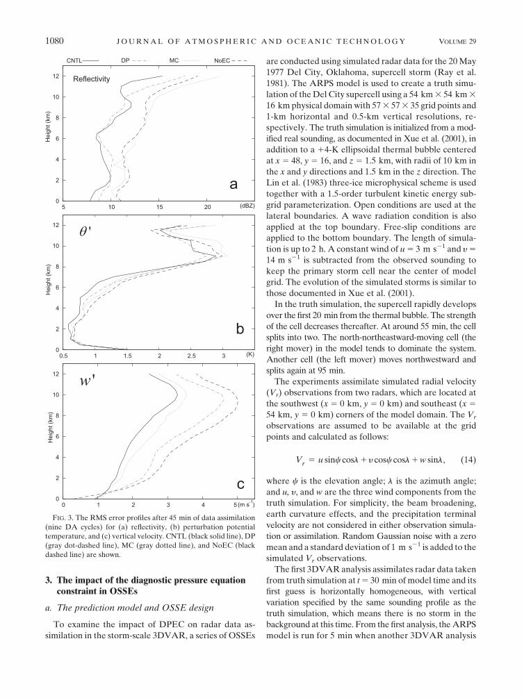
FIG. 3. The RMS error profiles after 45 min of data assimilation

(nine DA cycles) for (a) reflectivity, (b) perturbation potential

temperature, and (c) vertical velocity. CNTL (black solid line), DP

(gray dot-dashed line), MC (gray dotted line), and NoEC (black

dashed line) are shown.


is performed using the forecast as the background.

Such intermittent assimilation cycles are repeated every

5 min until 90 min, giving a data assimilation period of

60 min.

Table 1 lists all of the data assimilation experiments.

The first four experiments (CNTL, MC, DP, and NoEC)

are designed to investigate the impact of DPEC. For

comparison purposes, the impact of MCEC is also ex-

amined. Experiment CNTL includes both constraints

DPEC and MCEC. Experiment MC includes MCEC

only, while experiment DP includes DPEC only. In ex-

periment NoEC, neither DPEC nor MCEC is included.

The next four experiments, CNTLDm5, CNTLDd5,

CNTLDm25, and CNTLDd25, are designed to test the

sensitivity of the data assimilation to the DPEC weighting

coefficient. CNTLDm5 is the same as CNTL except that

the DP weighting coefficient used in CNTL is multiplied

by 5. In CNTLDd5, the DP weighting coefficient is di-

vided by 5. In CNTLDm25 and CNTLDd25, the co-

efficients are changed by a factor of 25.

The next four experiments, CNTLMm5, CNTLMd5,

CNTLMm25, and CNTLMd25, are designed to test the

sensitivity to the MCEC weighting coefficient. They are

the same as CNTL except that the MCEC weight is

changed by a factor of 5 or 25, following the same naming

convention as the DPEC sensitivity experiments.

To compare the accuracy of the data assimilation re-

sults from different experiments, the root-mean-squared

(RMS) error statistics of model variables between the

experiments and the truth simulation are computed as

RMS_s 5

ffiffiffiffiffiffiffiffiffiffiffiffiffiffiffiffiffiffiffiffiffiffiffiffiffiffiffiffi1

N�N

i51

(s 2 st)2i

s, (15)

where N is the total number of 3D grid points used in

the calculation, and the subscript t stands for the truth

simulation. The computation of the RMS error statistics

is only done over model grid points where the reflectivity

(calculated from the local hydrometeor mixing ratios) of

FIG. 4. The simulated reflectivity fields at z 5 6.5 km MSL for (a) the truth simulation experiments (b) NoEC, (c) DP, (d) MC, and

(e) CNTL; and the differences of the analyzed reflectivity from the truth at the same level for (f) NoEC, (g) DP, (h) MC, and (i) CNTL. All

fields are at 75-min model time or after 45 min of data assimilation.


the truth simulation is greater than 10 dBZ, which roughly

corresponds to storm region.

b. Results of OSSEs

To investigate the impact of DPEC, the RMS error

statistics are calculated during the whole assimilation

period for model variables, as shown in Fig. 2. For ease

of display, the RMS errors of simulated reflectivity are

shown in place of the errors for rain/snow/hail mixing

ratios, and the RMS error for the y wind component is

not shown, because it evolves similarly to the u wind

component.

From Fig. 2, it is seen that the errors are the lowest in

CNTL, where both DPEC and MCEC are included.

When only MCEC is included in MC, the errors are also

lower than those of NoEC and DP, but somewhat higher

than those of CNTL, especially during the earlier cycles.

Including DPEC only is less effective than including

MCEC only during the earlier cycles, but its accumu-

lated effects seem to exceed those of MCEC during the

later cycles in MC, especially for temperature and pres-

sure, which are most directly involved in the diagnostic

pressure equation (Figs. 1c,d). These results indicate that

including both DPEC and MCEC yields the best results

and the addition of DPEC has positive impacts.

To more clearly illustrate the impact of the two con-

straints, Fig. 3 shows the RMS error profiles after 45 min

of data assimilation (nine DA cycles). The RMS error of

reflectivity is evidently reduced in DP compared to

NoEC and in CNTL compared to MC, both of which are

due to the addition of DPEC. The largest difference in

reflectivity is over 4 dBZ between 6- and 8-km levels. At

most levels, the RMS errors of CNTL that includes both

constraints are the smallest among all four experiments.

For potential temperature, DP and CNTL generally pro-

duce smaller RMS error than NoEC and MC, respectively,

FIG. 5. The perturbation potential temperature at z 5 6.5 km MSL for (a) the truth simulation, (b) NoEC, (c) DP, (e) MC, and

(e) CNTL; and the difference of the temperature field between each data assimilation experiment and the truth simulation at z 5 6.5 km

MSL for (f) NoEC, (g) DP, (h) MC, and (i) CNTL. All the above plots are available at t 5 75 min into truth simulation (i.e., after 45-min

data assimilation).


with noticeable differences between 4 and 6.5 km, and

between 8.5 and 12 km (Fig. 3b). Figure 3c shows that

the additional use of DPEC in DP reduces the RMS

error of vertical velocity by about 0.4 m s21 at 10 km

MSL compared to NoEC, and similarly between CNTL

and MC (Fig. 3c). The use of MCEC reduces the w error

by over 1 m s21 near the 10-km level as shown by com-

paring MC and NoEC. The use of both equation con-

straints (CNTL) produces an error reduction of about

1.6 m s21 compared to the NoEC case at the same level.

The decrease in the vertical velocity RMS error by the

inclusion of equation constraints is very obvious above

the 1.5-km level.

To see the differences in the analyzed model fields,

we show in Figs. 3–5 the analyzed reflectivity, u9 and

w fields, and their differences from the truth, together with

the truth fields themselves, from the four experiments at

75 min of truth simulation time or 45 min into the data

assimilation. Figure 4 shows the reflectivity fields at 6.5 km

MSL. At this time, the reflectivity pattern for the right-

moving cell is recovered well in all four experiments.

Larger errors lie with the left-moving cell in the north-

western part of the domain and in the region between

the two cells, especially in NoEC and MC (Figs. 4f,h).

Experiments DP and CNTL, with the inclusion of DPEC,

are seen to produce better analyses of reflectivity than

NoEC and MC (cf. Figs. 4g, i versus Figs. 4f,h). Exper-

iment CNTL yields the best results in terms of the re-

flectivity error in the whole domain (Fig. 4i).

Figure 5 shows the corresponding analyzed u9 fields

and their differences from the truth. In general, the u9

field is recovered very well for both left- and right-moving

cells in all four experiments, and the pattern differences

among the experiments are relatively small at first glance.

However, from the difference fields, it can be clearly seen

that the use of DPEC only in DP mainly helps improve the

recovery of the temperature structure with the left-moving

cell (cf. Figs. 5g,f), and MCEC only in MC mainly helps

FIG. 6. The vertical velocity at z 5 6.0 km MSL for (a) the truth simulation, (b) CNTL, (d) NoEC, (e) DP, (f) MC; and the difference of

the vertical velocity between each data assimilation experiment and the truth simulation at z 5 6.0 km MSL for (c) CNTL, (g) NoEC,

(h) DP, and (i) MC. All the above plots are available at t 5 75 min into truth simulation (i.e., after 45-min data assimilation).


improve the temperature structure with the right-moving

cell (cf. Figs. 5h,f). As a whole, experiment CNTL with both

constraints again performs the best in terms of the analyzed

temperature structures for the whole storm system, given

the generally smaller temperature errors (Fig. 5i).

In Fig. 6, the corresponding w fields at z 5 6 km MSL

are shown. It is easily seen that the w structure associ-

ated with the right-moving storm cell is recovered well at

this time in all four experiments (Figs. 6b–e). For the

left-moving cell there are larger differences. Overall, CNTL

produces the best analysis of w field, and MC the second

best. Comparing the error fields, it is clear that MCEC has

a larger impact on the w analysis than DPEC, which is not

surprising because the mass continuity equation is mostly

responsible for linking w with the horizontal velocity com-

ponents, which are much better observed by the radars.

To summarize, both DPEC and MCEC built into the

3DVAR provide a positive impact on the analysis of

FIG. 7. The RMS error of model fields during the 1-h assimilation period for the (a) u

component of wind, (b) vertical velocity w, (c) perturbation potential temperature, (d) pres-

sure, (e) water vapor mixing ratio, (f) cloud water mixing ratio, (g) cloud ice mixing ratio, and

(h) simulated reflectivity from model rain/snow/hail mixing ratios. CNTL (black solid line),

CNTLDd5 (black dotted line), CNTLDm5 (gray short-dashed line), CNTLDd25 (gray dot-dashed

line), and CNTLDm25 (black long-dashed line) are shown.


a supercell storm system when assimilating radar radial

velocity data through intermittent assimilation cycles. The

impact of MCEC is clearer at the first several data as-

similation cycles, while the impact of DPEC is more ob-

vious in later cycles. Including both constraints at the

same time yields the best data assimilation results in most

model variables, especially for w and u, the hydrometeor

fields as represented by simulated reflectivity.

To test the sensitivity of the results to the weighting

coefficients of DPEC and MCEC, eight more sensitivity

experiments are conducted (Table 1). These experiments

are similar to CNTL, which uses both constraints, except

for the different values of their weight coefficients.

Figures 7and 8 show the evolution of the RMS errors of

these sensitivity experiments, as well as CNTL during

the 1-h data assimilation period for various model fields.

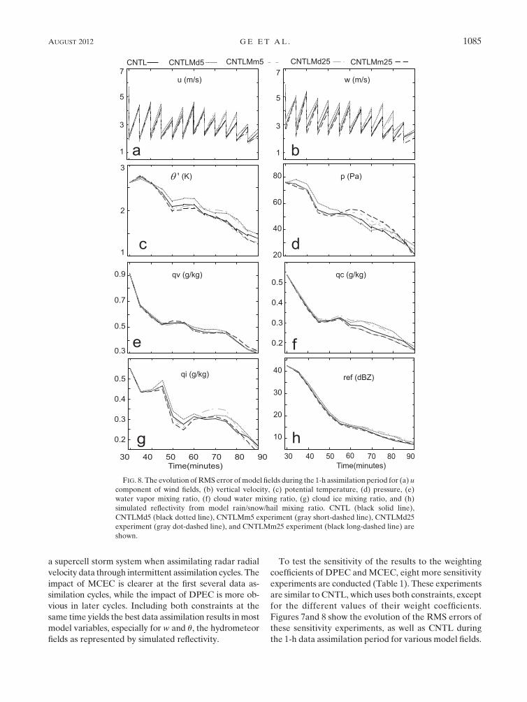
FIG. 8. The evolution of RMS error of model fields during the 1-h assimilation period for (a) u

component of wind fields, (b) vertical velocity, (c) potential temperature, (d) pressure, (e)

water vapor mixing ratio, (f) cloud water mixing ratio, (g) cloud ice mixing ratio, and (h)

simulated reflectivity from model rain/snow/hail mixing ratio. CNTL (black solid line),

CNTLMd5 (black dotted line), CNTLMm5 experiment (gray short-dashed line), CNTLMd25

experiment (gray dot-dashed line), and CNTLMm25 experiment (black long-dashed line) are

shown.


The sensitivity to the DPEC weighting coefficient is

shown in Fig. 7. When the DPEC weighting coefficient is

increased or decreased by a factor of 5, the RMS errors

are not changed much compared to those of CNTL for

all model variables. When the DPEC weighting coefficient

is decreased by a factor of 25, the RMS errors are still not

too different. However, when the DPEC weighting co-

efficient is increased by a factor of 25, the RMS errors

become significantly larger than those of CNTL, especially

for u, w, pressure, and u; their errors even increase with the

data assimilation cycles (Figs. 7a–d). This indicates that

one should be cautious in choosing the DPEC weighting

coefficient. A very large weighting coefficient should be

avoided, because it might give DPEC much more of the

total cost function and then degrade the quality of the

data assimilation.

Figure 8 presents the sensitivity to the MCEC weighting

coefficient. When the weighting coefficient is increased

or decreased by a factor of 5, the RMS errors are not

changed much. When the weighting coefficient is changed

by a factor of 25, the RMS errors are increased somewhat

in later assimilation cycles for temperature, pressure, and

cloud water and ice mixing ratios (Figs. 8d–g). Therefore,

it can be concluded that the mass continuity equation

constraint is not very sensitive to the weighting coefficient

within reasonable range.

In summary, in this section, we demonstrated the positive

impact of DPEC and MCEC in the 3DVAR system with

simulated radar data. It was found that the data assimilation

results are the best when both constraints are utilized. In

next section, we examine the impact of DPEC using a real

case.

4. The 5 May 2007 Greensburg tornadic supercellstorm case

The 5 May 2007 Greensburg, Kansas, tornadic thun-

derstorm complex produced 18 tornadoes in the Dodge

City forecast area and 47 tornado reports in Kansas,

Nebraska, and Missouri. One of them is the strongest

tornadoes in recent years. This tornado started moving

through Greensburg at 0245 UTC 5 May 2007 [2145

central daylight time CDT) 4 May] and destroyed over

90% of the town. The tornado damage was rated at

EF5—the highest rating on the enhanced Fujita scale

(McCarthy et al. 2007). A detail description of the su-

percell that spawned this tornado and its environment

setting can be found in Stensrud and Gao (2010).

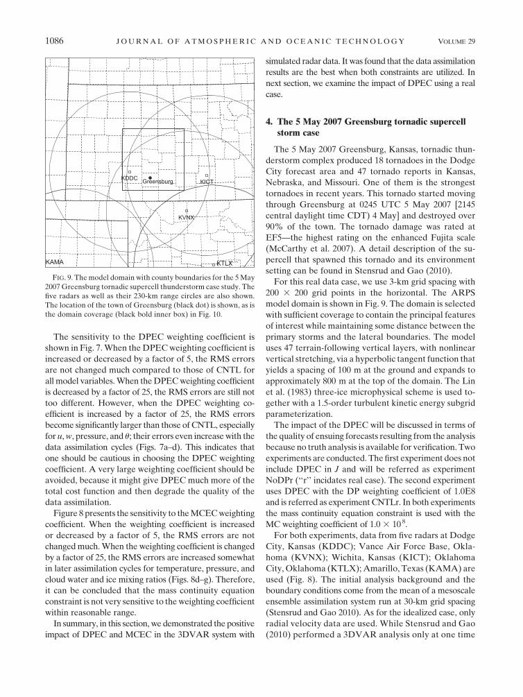
For this real data case, we use 3-km grid spacing with

200 3 200 grid points in the horizontal. The ARPS

model domain is shown in Fig. 9. The domain is selected

with sufficient coverage to contain the principal features

of interest while maintaining some distance between the

primary storms and the lateral boundaries. The model

uses 47 terrain-following vertical layers, with nonlinear

vertical stretching, via a hyperbolic tangent function that

yields a spacing of 100 m at the ground and expands to

approximately 800 m at the top of the domain. The Lin

et al. (1983) three-ice microphysical scheme is used to-

gether with a 1.5-order turbulent kinetic energy subgrid

parameterization.

The impact of the DPEC will be discussed in terms of

the quality of ensuing forecasts resulting from the analysis

because no truth analysis is available for verification. Two

experiments are conducted. The first experiment does not

include DPEC in J and will be referred as experiment

NoDPr (‘‘r’’ incidates real case). The second experiment

uses DPEC with the DP weighting coefficient of 1.0E8

and is referred as experiment CNTLr. In both experiments

the mass continuity equation constraint is used with the

MC weighting coefficient of 1.0 3 10 8.

For both experiments, data from five radars at Dodge

City, Kansas (KDDC); Vance Air Force Base, Okla-

homa (KVNX); Wichita, Kansas (KICT); Oklahoma

City, Oklahoma (KTLX); Amarillo, Texas (KAMA) are

used (Fig. 8). The initial analysis background and the

boundary conditions come from the mean of a mesoscale

ensemble assimilation system run at 30-km grid spacing

(Stensrud and Gao 2010). As for the idealized case, only

radial velocity data are used. While Stensrud and Gao

(2010) performed a 3DVAR analysis only at one time

FIG. 9. The model domain with county boundaries for the 5 May

2007 Greensburg tornadic supercell thunderstorm case study. The

five radars as well as their 230-km range circles are also shown.

The location of the town of Greensburg (black dot) is shown, as is

the domain coverage (black bold inner box) in Fig. 10.


level before the launch of the forecast, the present study

performs cycled 3DVAR analyses with a 1-h-long as-

similation period before the forecast. A 5-min ARPS

forecast follows each analysis, and this process is repeated

until the end of the 1-h assimilation period. From the final

analysis, a 1-h forecast is launched. Thus, each experi-

ment consisted of a 1-h assimilation period (from 0130 to

0230 UTC) and a 1-h forecast period (0230–0330 UTC).

The radar reflectivity mosaic from the aforementioned

five WSR-88D radars is used for forecast verification. The

evolution of the storm as indicated by the radar reflectivity

mosaic at 2 km MSL is shown in Fig. 10 from 0230 to

0330 UTC every 20 min. We focus on the discussion of the

major supercell thunderstorm at the southernmost side

that produces the EF-5 tornado hitting the Greensburg

area between 0245 and ;0305 UTC. It bears a hook echo

signature at 0230 UTC (Fig. 10a). As the major storm

reaches Greensburg, the hook echo signature becomes

less prominent (Figs. 10b,c) due to reflectivity wrap up.

During this period, the radar velocity observations (not

shown) indicate strong cyclonic rotation associated with

the strong tornado. The major storm moves gradually

toward northeast. After passing the town of Greensburg,

the storm maintains a visible hook echo and continues to

move to the northeast. A second EF-3 tornado develops

at the end of Greensburg tornado just northeast of the

town (McCarthy et al. 2007).

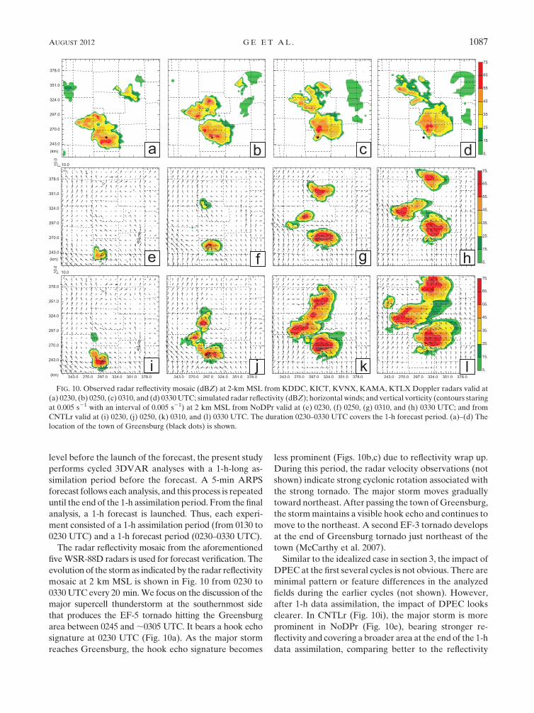
Similar to the idealized case in section 3, the impact of

DPEC at the first several cycles is not obvious. There are

minimal pattern or feature differences in the analyzed

fields during the earlier cycles (not shown). However,

after 1-h data assimilation, the impact of DPEC looks

clearer. In CNTLr (Fig. 10i), the major storm is more

prominent in NoDPr (Fig. 10e), bearing stronger re-

flectivity and covering a broader area at the end of the 1-h

data assimilation, comparing better to the reflectivity

FIG. 10. Observed radar reflectivity mosaic (dBZ) at 2-km MSL from KDDC, KICT, KVNX, KAMA, KTLX Doppler radars valid at

(a) 0230, (b) 0250, (c) 0310, and (d) 0330 UTC; simulated radar reflectivity (dBZ); horizontal winds; and vertical vorticity (contours staring

at 0.005 s21 with an interval of 0.005 s21) at 2 km MSL from NoDPr valid at (e) 0230, (f) 0250, (g) 0310, and (h) 0330 UTC; and from

CNTLr valid at (i) 0230, (j) 0250, (k) 0310, and (l) 0330 UTC. The duration 0230–0330 UTC covers the 1-h forecast period. (a)–(d) The

location of the town of Greensburg (black dots) is shown.


observation (Fig. 10a). North of the major storm, a storm

cell also develops in CNTLr (Fig. 10i), although it is much

weaker than observed (Fig. 10a). At the upper levels, this

cell is better developed (not shown). In comparison,

NoDPr completely misses this cell at this time. Based on

these results, we can say that the inclusion of DPEC does

help improve the storm analysis, consistent with our

earlier OSSE results.

From the improved analysis, a better forecast should

be expected. Forecasts are launched from each of the

above two analyses. After 20 min of forecast at 0250 UTC,

the major storm cell in CNTLr strengthens and develops

a hook echo signature with a clearly defined vorticity center

while two more cells are fully developed to its north and

northwest (Fig. 10j), more or less matching the obser-

vation (Fig. 10b). On the other hand, the primary cell in

NoDPr is weaker and the matching northwest cells are

completely absent (Fig. 10f). During the next 20 min

until 0310 UTC, the primary cell in CNTLr develops

further and shows a clearer hook echo signature (Fig.

10k). Overall, the intensity of the cells is overpredicted,

which may have to do with model error or error in the

storm environment. Stensrud and Gao (2010) found strong

sensitivity of the forecast to the storm environment, while

Dawson et al. (2010) had shown the large sensitivity of

predicted storm to microphysics parameterization. The

cells in NoDPr are generally weaker (Fig. 10g), but do

not necessarily show a better match to the observation

(Fig. 10c). By the end of the 1-h forecast period, the major

storm is predicted well in both CNTLr and NoDPr in

terms of its moving path and general rainfall coverage.

Both experiments overpredict the northern cells. To

quantitatively evaluate the above two forecasts, equi-

table threat scores (ETSs) for reflectivity at 2.1 km MSL

(with the 15-dBZ threshold) are computed and plotted

in Fig. 11. It is seen that CNTLr (dashed line) yields

higher scores than NoDPr (solid line), which agrees with

our subjective assessment above.

To further examine the difference in the two forecasts,

the maximum vertical vorticity (z) below 2 km MSL is

computed from the forecasts every minute. The time

series of the z are plotted in Fig. 12. It is shown that

CNTLr (dashed line) predicts larger low-level maximum

z than NoDPr (solid line) during the entire forecast pe-

riod, especially during the last half-hour. A larger low-

level z usually indicates stronger and deeper mesocyclone

rotation. As an example, Fig. 13 shows z in a vertical cross

section through the low-level maximum z center of the

major storm at y 5 253.5 km at 0250 UTC for both ex-

periments. It can be seen that CNTLr (Fig. 13b) predicts

a stronger and deeper rotating column than NoDPr (Fig.

13a). Considering that this is a strong tornadic supercell,

we believe the forecast of CNTLr is more accurate.

5. Summary and conclusions

Storm-scale 3DVAR is computationally efficient and

operationally feasible for assimilating full-volume Doppler

radar data for the prediction of thunderstorms. However,

it is often challenged as being less optimal for the storm-

scale application because of its use of static background

error covariance and lack of balance among analyzed

model variables. To reduce this problem, we proposed to

incorporate into the ARPS 3DVAR cost function a weak

constraint based on the diagnostic pressure equation

derived from the full ARPS momentum equations. The

main goal is to help improve dynamic consistency among

model variables and therefore improve the analysis of

convective storms and their subsequent forecast.

FIG. 11. Equitable threat scores of predicted reflectivity at

2.1 km MSL with 15-dBZ thresholds. NoDPr (solid line) and

CNTLr (dashed line) are shown.

FIG. 12. The time series of maximum vertical vorticities below

2 km from 0230 to 0330 UTC 5 May 2007 every 1 min. The hori-

zontal axis shows the time (UTC), the vertical axis shows the ver-

tical vorticity value (s21). Experiments NoDPr (solid line) and

CNTLr (dashed line) are shown.


The impact of DPEC is first investigated using an ide-

alized tornadic supercell thunderstorm through OSSEs.

A 1-h data assimilation period is used through 5-min in-

termittent assimilation cycles and radar radial velocity

observations from two assumed radars that are used in all

the experiments. For comparison purpose, the impact of

MCEC already contained in the ARPS 3DVAR is also

examined.

The DPEC is found in the OSSEs to have small im-

pacts during the first several data assimilation cycles when

MCEC is seen to have larger impacts. However, the im-

pact of DPEC becomes more pronounced during the later

cycles. Including both DPEC and MCEC in the 3DVAR

cost function is found to yield the best analysis of the

storm. Sensitivity experiments on the weighting coefficients

show that DPEC is not very sensitive to the choice of its

weighting coefficient, and the coefficient can be increased

or decreased by a factor of 5 without too much effect on

the assimilation results. However, large DPEC weight

(increase by a factor of 25 in our idealized case) should

be avoided because it gives DPEC too much of the total

J and evidently degrades data assimilation results.

The new ARPS 3DVAR system with DPEC is further

applied to the 5 May 2007 Greensburg tornadic super-

cell storm. The use of DPEC in this real case is shown to

speed up the spinup of convective cells during the in-

termittent data assimilation process, and improve the en-

suing forecast in terms of the general evolution of storm

cells and the low-level rotation near the time of observed

tornado.

Overall, the additional DPEC in the ARPS 3DVAR

system has positive impacts on storm-scale 3DVAR data

assimilation of Doppler radar data, and on the subsequent

forecast. In the future, the system will be tested with more

real data cases to hopefully demonstrate the robustness of

the conclusions.

Acknowledgments. This work was supported by NSF

Grants ATM-0331756, ATM-0738370, NSF ATM-

0530814, NSF AGS-0802888, and NOAA’s Warn-on-

Forecast Project. The third author was also supported by

NSF OCI-0905040, AGS-0941491, and AGS-1046171.

Robin Tanamachi kindly provided the manually deal-

iased radial velocity dataset of the Dodge City, Kansas

(KDDC) radar. Computations were performed at the

Pittsburgh Supercomputing Center (PSC) and Oklahoma

Supercomputing Center for Research and Education

(OSCER). We appreciate three anonymous reviewers for

their very thoughtful comments, which helped signifi-

cantly improve the quality of this paper from its original

form.

APPENDIX

List of Acronyms and Variables

3DVAR Three-dimensional variational data

assimilation

4DVAR Four-dimensional variational data

assimilation

ARPS Advanced Regional Prediction System

CDT Central Daylight Time

DA Data assimilation

DPEC Diagnostic pressure equation constraint

EF Enhanced Fujita scale

EnKF Ensemble Kalman filter

ETS Equitable threat scores

MCEC Mass continuity equation constraint

FIG. 13. The vertical vorticity (10–5 s21) at the vertical cross section through the center of the major storm at

y 5 253.5 km at 0250 UTC 5 May 2007 for the (a) NoDPr and (b) CNTLr.


MM5 Fifth-generation Pennsylvania State Uni-

versity (PSU)–National Center for At-

mospheric Research (NCAR) Mesoscale

ModelNWP Numerical weather prediction

OSSE Observational System Simulation Experi-

mentRHS Right-hand side

RMS Root-mean square

WSR-88D Weather Surveillance Radar-1988

Doppler (radar)

J Total cost function

Jb Background term in the total cost function

Jo Observation term in the total cost function

Jc Equation constraint term in the total cost

functionx Analysis vector

xb Background vector

B Background error covariance matrices

H Observation forward operator

yo Observation vector

R Observation error covariance matrices

dx Analysis increment vector

V Analysis vector (in incremental form cost

function)

(. . .)T Transpose operator

u u component wind (in x direction)

y y component wind (in y direction)

w Vertical velocity

u Potential temperature

p Pressure

qv Water vapor mixing ratio

Q MCEC

P DPEC

$ Gradient operator

� Dot product operator

E Forcing term of the vector Euclidian mo-

mentum equations

=2 Laplace operator

(� � �)9 Deviation from the base state

� � �)ð Base state

V Wind vector

g Gravitational constant

› Partial derivative operator

cs Acoustic wave speed

« Ratio of the gas constants for day air and

water vapor

qliquid1ice Mixing ratios for precipitations in liquid

and ice phases

C Coriolis force vector

D The vector containing subgrid scale turbu-

lence and computational mixing termsi Unit vector in x direction

j Unit vector in y direction

k Unit vector in z direction

f Coriolis coefficient~f Coriolis coefficient

V Angular velocity of the earth

f Latitude

O(. . .) Big O notation

k. . .k Euclidean norm

Vr Radial velocity

c Elevation angle of a radar beam

REFERENCES

Aksoy, A., D. C. Dowell, and C. Snyder, 2009: A multicase com-

parative assessment of the ensemble Kalman filter for assim-

ilation of radar observations. Part I: Storm-scale analyses.

Mon. Wea. Rev., 137, 1805–1824.

——, ——, and ——, 2010: A multicase comparative assessment of

the ensemble Kalman filter for assimilation of radar obser-

vations. Part II: Short-range ensemble forecasts. Mon. Wea.

Rev., 138, 1273–1292.

Buehner, M., 2005: Ensemble-derived stationary and flow-

dependent background-error covariances: Evaluation in a

quasi-operational NWP setting. Quart. J. Roy. Meteor. Soc.,

131, 1013–1043.

Caya, A., J. Sun, and C. Snyder, 2005: A comparison between the

4D-VAR and the ensemble Kalman filter techniques for radar

data assimilation. Mon. Wea. Rev., 133, 3081–3094.

Crook, N. A., 1994: Numerical simulations initialized with radar-

derived winds. Part I: Simulated data experiments. Mon. Wea.

Rev., 122, 1189–1203.

——, and J. D. Tuttle, 1994: Numerical simulations initialized with

radar-derived winds. Part II: Forecasts of three gust front ca-

ses. Mon. Wea. Rev., 122, 1214–1217.

Dawson, D. T., II, M. Xue, J. A. Milbrandt, and M. K. Yau, 2010:

Comparison of evaporation and cold pool development be-

tween single-moment and multi-moment bulk microphysics

schemes in idealized simulations of tornadic thunderstorms.

Mon. Wea. Rev., 138, 1152–1171.

Dowell, D. C., L. J. Wicker, and C. Snyder, 2011: Ensemble Kal-

man filter assimilation of radar observations of the 8 May 2003

Oklahoma City supercell: Influences of reflectivity observa-

tions on storm-scale analyses. Mon. Wea. Rev., 139, 272–294.

Gal-Chen, T., 1978: A method for the initialization of the anelastic

equations: Implications for matching models with observa-

tions. Mon. Wea. Rev., 106, 587–606.

Gao, J.-D., M. Xue, A. Shapiro, and K. K. Droegemeier, 1999: A

variational method for the analysis of three-dimensional wind

fields from two Doppler radars. Mon. Wea. Rev., 127, 2128–2142.

——, ——, ——, Q. Xu, and K. K. Droegemeier, 2001: Three-

dimensional simple adjoint velocity retrievals from single

Doppler radar. J. Atmos. Oceanic Technol., 18, 26–38.

——, ——, K. Brewster, and K. K. Droegemeier, 2004: A three-

dimensional variational data analysis method with recursive

filter for Doppler radars. J. Atmos. Oceanic Technol., 21, 457–

469.

Hamill, T. M., and C. Snyder, 2000: A hybrid ensemble Kalman

filter–3D variational analysis scheme. Mon. Wea. Rev., 128,2905–2919.

Hane, C. E., and B. C. Scott, 1978: Temperature and pressure

perturbations within convective clouds derived from detailed


air motion information: Preliminary testing. Mon. Wea. Rev.,

106, 654–661.

Hu, M., and M. Xue, 2007a: Analysis and prediction of 8 May 2003

Oklahoma City tornadic thunderstorm and embedded tor-

nado using ARPS with assimilation of WSR-88D radar data.

Preprints, 22nd Conf. on Weather Analysis and Forecasting/

18th Conf. on Numerical Weather Prediction, Salt Lake City,

UT, Amer. Meteor. Soc., 1B.4. [Available online at http://

ams.confex.com/ams/pdfpapers/123683.pdf.]

——, and ——, 2007b: Impact of configurations of rapid in-

termittent assimilation of WSR-88D radar data for the 8 May

2003 Oklahoma City tornadic thunderstorm case. Mon. Wea.

Rev., 135, 507–525.

——, ——, and K. Brewster, 2006a: 3DVAR and cloud analysis

with WSR-88D level-II data for the prediction of Fort Worth

tornadic thunderstorms. Part I: Cloud analysis and its impact.

Mon. Wea. Rev., 134, 675–698.

——, ——, J. Gao, and K. Brewster, 2006b: 3DVAR and cloud

analysis with WSR-88D level-II data for the prediction of Fort

Worth tornadic thunderstorms. Part II: Impact of radial ve-

locity analysis via 3DVAR. Mon. Wea. Rev., 134, 699–721.

Ide, K., P. Courtier, M. Ghil, and A. Lorenc, 1997: Unified notation

for data assimilation: Operational, sequential and variational.

J. Meteor. Soc. Japan, 75, 181–189.

Li, Y., X. Wang, and M. Xue, 2012: Assimilation of radar radial

velocity data with the WRF ensemble-3DVAR hybrid system

for the prediction of Hurricane Ike (2008). Mon. Wea. Rev.,

in press.

Lin, Y.-L., R. D. Farley, and H. D. Orville, 1983: Bulk parame-

terization of the snow field in a cloud model. J. Climate Appl.

Meteor., 22, 1065–1092.

Liou, Y.-C., 2001: The derivation of absolute potential temperature

perturbations and pressure gradients from wind measure-

ments in three-dimensional space. J. Atmos. Oceanic Technol.,

18, 577–590.

——, and Y.-J. Chang, 2009: A variational multiple–Doppler radar

three-dimensional wind synthesis method and its impacts on

thermodynamic retrieval. Mon. Wea. Rev., 137, 3992–4010.

——, T.-C. C. Wang, and K.-S. Chung, 2003: A three-dimensional

variational approach for deriving the thermodynamic struc-

ture using Doppler wind observations—An application to

a subtropical squall line. J. Appl. Meteor., 42, 1443–1454.

Liu, H., and M. Xue, 2006: Retrieval of moisture from slant-path

water vapor observations of a hypothetical GPS network using

a three-dimensional variational scheme with anisotropic

background error. Mon. Wea. Rev., 134, 933–949.

——, ——, R. J. Purser, and D. F. Parrish, 2007: Retrieval of

moisture from simulated GPS slant-path water vapor obser-

vations using 3DVAR with anisotropic recursive filters. Mon.

Wea. Rev., 135, 1506–1521.

Lorenc, A., 2003: The potential of the ensemble Kalman filter for

NWP—A comparison with 4D-Var. Quart. J. Roy. Meteor.

Soc., 129, 3183–3203.

McCarthy, D., L. Ruthi, and J. Hutton, 2007: The Greensburg, KS

tornado. Preprints, 22th Conf. on Weather Analysis and

Forecasting and 18th Conf. on Numerical Weather Prediction,

Park City, UT, Amer. Meteor. Soc., J2.4. [Available online at

http://ams.confex.com/ams/pdfpapers/126927.pdf.]

Protat, A., and I. Zawadzki, 2000: Optimization of dynamic re-

trievals from a multiple-Doppler radar network. J. Atmos.

Oceanic Technol., 17, 753–760.

——, ——, and A. Caya, 2001: Kinematic and thermodynamic

study of a shallow hailstorm sampled by the McGill bistatic

multiple-Doppler radar network. J. Atmos. Sci., 58, 1222–

1248.

Purser, R. J., W.-S. Wu, D. F. Parrish, and N. M. Roberts, 2003a:

Numerical aspects of the application of recursive filters to

variational statistical analysis. Part I: Spatially homogeneous

and isotropic Gaussian covariances. Mon. Wea. Rev., 131,

1524–1535.

——, ——, ——, and ——, 2003b: Numerical aspects of the ap-

plication of recursive filters to variational statistical analysis.

Part II: Spatially inhomogeneous and anisotropic general co-

variances. Mon. Wea. Rev., 131, 1536–1548.

Ray, P. S., and Coauthors, 1981: The morphology of severe tor-

nadic storms on 20 May 1977. J. Atmos. Sci., 38, 1643–1663.

Snook, N., M. Xue, and Y. Jung, 2011: Analysis of a tornadic me-

soscale convective vortex based on ensemble Kalman filter

assimilation of CASA X-band and WSR-88D radar data. Mon.

Weat. Rev., 139, 3446–3468.

Snyder, C., and F. Zhang, 2003: Assimilation of simulated Doppler

radar observations with an ensemble Kalman filter. Mon. Wea.

Rev., 131, 1663–1677.

Stensrud, D. J., and J. Gao, 2010: Importance of horizontally in-

homogeneous environmental initial conditions to ensemble

storm-scale radar data assimilation and very short-range

forecasts. Mon. Wea. Rev., 138, 1250–1272.

Sun, J., 2005: Initialization and numerical forecasting of a supercell

storm observed during STEPS. Mon. Wea. Rev., 133, 793–813.

——, and N. A. Crook, 1997: Dynamical and microphysical re-

trieval from Doppler radar observations using a cloud model

and its adjoint. Part I: Model development and simulated data

experiments. J. Atmos. Sci., 54, 1642–1661.

——, and ——, 1998: Dynamical and microphysical retrieval from

Doppler radar observations using a cloud model and its ad-

joint. Part II: Retrieval experiments of an observed Florida

convective storm. J. Atmos. Sci., 55, 835–852.

——, and ——, 2001: Real-time low-level wind and temperature

analysis using single WSR-88D data. Wea. Forecasting, 16,

117–132.

——, D. W. Flicker, and D. K. Lilly, 1991: Recovery of three-di-

mensional wind and temperature fields from single-Doppler

radar data. J. Atmos. Sci., 48, 876–890.

Tong, M., and M. Xue, 2005: Ensemble Kalman filter assimila-

tion of Doppler radar data with a compressible non-

hydrostatic model: OSS experiments. Mon. Wea. Rev., 133,

1789–1807.

Wang, X., D. M. Barker, C. Snyder, and T. M. Hamill, 2008a: A

hybrid ETKF-3DVAR data assimilation scheme for the WRF

model. Part I: Observing system simulation experiment. Mon.

Wea. Rev., 136, 5116–5131.

——, ——, ——, and ——, 2008b: A hybrid ETKF-3DVAR data

assimilation scheme for the WRF model. Part II: Real obser-

vation experiment. Mon. Wea. Rev., 136, 5132–5147.

Wang, Z., 1993: Variational data assimilation with 2-D shallow

water equations and 3-D FSU global spectral models. Dis-

sertation, Department of Mathematics, Florida State Uni-

versity, 224 pp.

Weygandt, S. S., A. Shapiro, and K. K. Droegemeier, 2002a: Re-

trieval of model initial fields from single-Doppler observations

of a supercell thunderstorm. Part I: Single-Doppler velocity

retrieval. Mon. Wea. Rev., 130, 433–453.

——, ——, and ——, 2002b: Retrieval of model initial fields from

single-Doppler observations of a supercell thunderstorm. Part

II: Thermodynamic retrieval and numerical prediction. Mon.

Wea. Rev., 130, 454–476.


Xiao, Q., Y.-H. Kuo, J. Sun, W.-C. Lee, E. Lim, Y.-R. Guo, and D. M.

Barker, 2005: Assimilation of Doppler radar observations with

a regional 3DVAR system: Impact of Doppler velocities on

forecasts of a heavy rainfall case. J. Appl. Meteor., 44, 768–788.

Xu, Q., H. Gu, and S. Yang, 2001: Simple adjoint method for three-

dimensional wind retrievals from single-Doppler radar. Quart.

J. Roy. Meteor. Soc., 127, 1053–1068.

Xue, M., K. K. Droegemeier, and V. Wong, 2000: The Advanced

Regional Prediction System (ARPS)—A multiscale non-

hydrostatic atmospheric simulation and prediction tool. Part I:

Model dynamics and verification. Meteor. Atmos. Phys., 75,

161–193.

——, and Coauthors, 2001: The Advanced Regional Prediction

System (ARPS)—A multi-scale nonhydrostatic atmospheric

simulation and prediction tool. Part II: Model physics and

applications. Meteor. Atmos. Phys., 76, 143–166.

——, D.-H. Wang, J.-D. Gao, K. Brewster, and K. K. Droegemeier,

2003: The Advanced Regional Prediction System (ARPS),

storm-scale numerical weather prediction and data assimila-

tion. Meteor. Atmos. Phys., 82, 139–170.

——, M. Tong, and K. K. Droegemeier, 2006: An OSSE framework

based on the ensemble square-root Kalman filter for evalu-

ating impact of data from radar networks on thunderstorm

analysis and forecast. J. Atmos. Oceanic Technol., 23, 46–66.

——, and Coauthors, 2008: CAPS realtime storm-scale ensemble

and high-resolution forecasts as part of the NOAA Hazardous

Weather Testbed 2008 Spring Experiment. Preprints, 24th

Conf. Several Local Storms, Savannah, GA, Amer. Meteor.

Soc., 12.12. [Available online at http://ams.confex.com/ams/

pdfpapers/142036.pdf.]

——, and Coauthors, 2011: Realtime convection-permitting ensemble

and convection-resolving deterministic forecasts of CAPS for the

hazardous weather testbed 2010 spring experiment. Preprints,

24th Conf. Weather Forecasting/20th Conf. Numerical Weather

Prediction, Seattle, WA, Amer. Meteor. Soc., 9A.2. [Available

online at http://ams.confex.com/ams/91Annual/webprogram/

Manuscript/Paper183227/Xue_CAPS_2011_SpringExperiment_

24thWAF20thNWP_ExtendedAbstract.pdf.]

Zhang, F., C. Snyder, and J. Sun, 2004: Impacts of initial estimate

and observations on the convective-scale data assimilation

with an ensemble Kalman filter. Mon. Wea. Rev., 132, 1238–

1253.

——, Y. Weng, J. A. Sippel, Z. Meng, and C. H. Bishop, 2009:

Cloud-resolving hurricane initialization and prediction

through assimilation of Doppler radar observations with an

ensemble Kalman filter. Mon. Wea. Rev., 137, 2105–2125.

Zhao, Q., J. Cook, Q. Xu, and P. R. Harasti, 2006: Using radar wind

observations to improve mesoscale numerical weather pre-

diction. Wea. Forecasting, 21, 502–522.

——, ——, ——, and ——, 2008: Improving short-term storm

predictions by assimilating both radar radial-wind and re-

flectivity observations. Wea. Forecasting, 23, 373–391.


Documents

Diagnostic Pressure Equation as a Weak Constraint in a