Differential Equations 1 - Second Part

The Heat Equation

Lecture Notes - 2011 - 11th March

Universita di Padova

Roberto Monti

Contents

Chapter 1. Heat Equation 51. Introduction 52. The foundamental solution and its properties 63. Parabolic mean formula 144. Parabolic maximum principles 165. Regularity of local solutions and Cauchy estimates 196. Harnack inequality 22

Chapter 2. Maximum principles 231. Maximum principle for elliptic-parabolic operators 232. Hopf Lemma 243. Strong maximum principle 26

3

CHAPTER 1

Heat Equation

1. Introduction

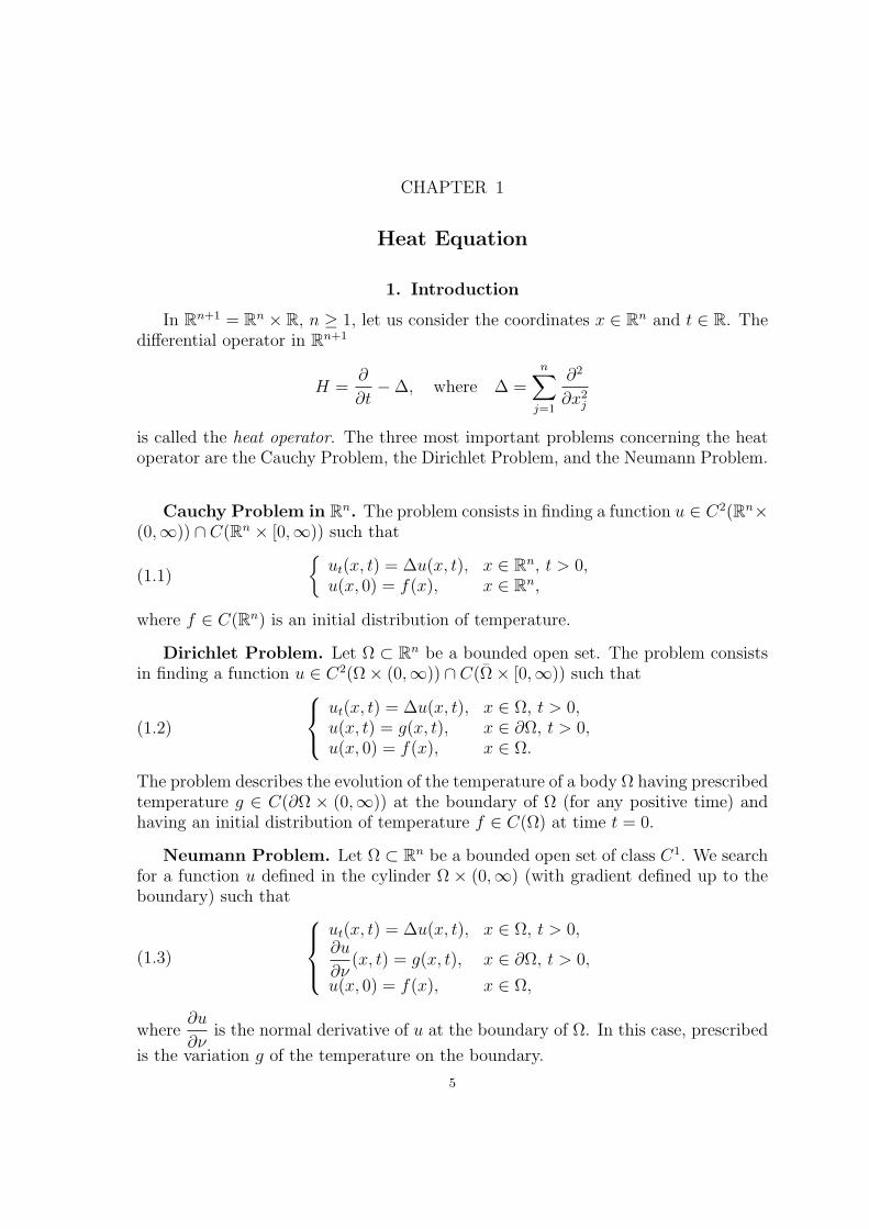
In Rn+1 = Rn × R, n ≥ 1, let us consider the coordinates x ∈ Rn and t ∈ R. Thedifferential operator in Rn+1

H =∂

∂t−∆, where ∆ =

n∑j=1

∂2

∂x2j

is called the heat operator. The three most important problems concerning the heatoperator are the Cauchy Problem, the Dirichlet Problem, and the Neumann Problem.

Cauchy Problem in Rn. The problem consists in finding a function u ∈ C2(Rn×(0,∞)) ∩ C(Rn × [0,∞)) such that

(1.1)

ut(x, t) = ∆u(x, t), x ∈ Rn, t > 0,u(x, 0) = f(x), x ∈ Rn,

where f ∈ C(Rn) is an initial distribution of temperature.

Dirichlet Problem. Let Ω ⊂ Rn be a bounded open set. The problem consistsin finding a function u ∈ C2(Ω× (0,∞)) ∩ C(Ω× [0,∞)) such that

(1.2)

ut(x, t) = ∆u(x, t), x ∈ Ω, t > 0,u(x, t) = g(x, t), x ∈ ∂Ω, t > 0,u(x, 0) = f(x), x ∈ Ω.

The problem describes the evolution of the temperature of a body Ω having prescribedtemperature g ∈ C(∂Ω × (0,∞)) at the boundary of Ω (for any positive time) andhaving an initial distribution of temperature f ∈ C(Ω) at time t = 0.

Neumann Problem. Let Ω ⊂ Rn be a bounded open set of class C1. We searchfor a function u defined in the cylinder Ω × (0,∞) (with gradient defined up to theboundary) such that

(1.3)

ut(x, t) = ∆u(x, t), x ∈ Ω, t > 0,∂u

∂ν(x, t) = g(x, t), x ∈ ∂Ω, t > 0,

u(x, 0) = f(x), x ∈ Ω,

where∂u

∂νis the normal derivative of u at the boundary of Ω. In this case, prescribed

is the variation g of the temperature on the boundary.

5

6 1. HEAT EQUATION

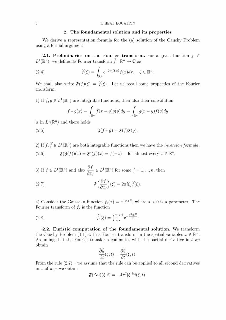
2. The foundamental solution and its properties

We derive a representation formula for the (a) solution of the Cauchy Problemusing a formal argument.

2.1. Preliminaries on the Fourier transform. For a given function f ∈L1(Rn), we define its Fourier transform f : Rn → C as

(2.4) f(ξ) =

∫Rn

e−2πi〈ξ,x〉f(x)dx, ξ ∈ Rn.

We shall also write F(f)(ξ) = f(ξ). Let us recall some properties of the Fouriertransform.

1) If f, g ∈ L1(Rn) are integrable functions, then also their convolution

f ∗ g(x) =

∫Rnf(x− y)g(y)dy =

∫Rng(x− y)f(y)dy

is in L1(Rn) and there holds

(2.5) F(f ∗ g) = F(f)F(g).

2) If f, f ∈ L1(Rn) are both integrable functions then we have the inversion formula:

(2.6) F(F(f))(x) = F2(f)(x) = f(−x) for almost every x ∈ Rn.

3) If f ∈ L1(Rn) and also∂f

∂xj∈ L1(Rn) for some j = 1, ..., n, then

(2.7) F( ∂f∂xj

)(ξ) = 2πiξj f(ξ).

4) Consider the Gaussian function fs(x) = e−s|x|2, where s > 0 is a parameter. The

Fourier transform of fs is the function

(2.8) fs(ξ) =(πs

)n2e−

π2|ξ|2s .

2.2. Euristic computation of the foundamental solution. We transformthe Cauchy Problem (1.1) with a Fourier transform in the spatial variables x ∈ Rn.Assuming that the Fourier transform commutes with the partial derivative in t weobtain

∂u

∂t(ξ, t) =

∂u

∂t(ξ, t).

From the rule (2.7) – we assume that the rule can be applied to all second derivativesin x of u, – we obtain

F(∆u)(ξ, t) = −4π2|ξ|2u(ξ, t).

2. THE FOUNDAMENTAL SOLUTION AND ITS PROPERTIES 7

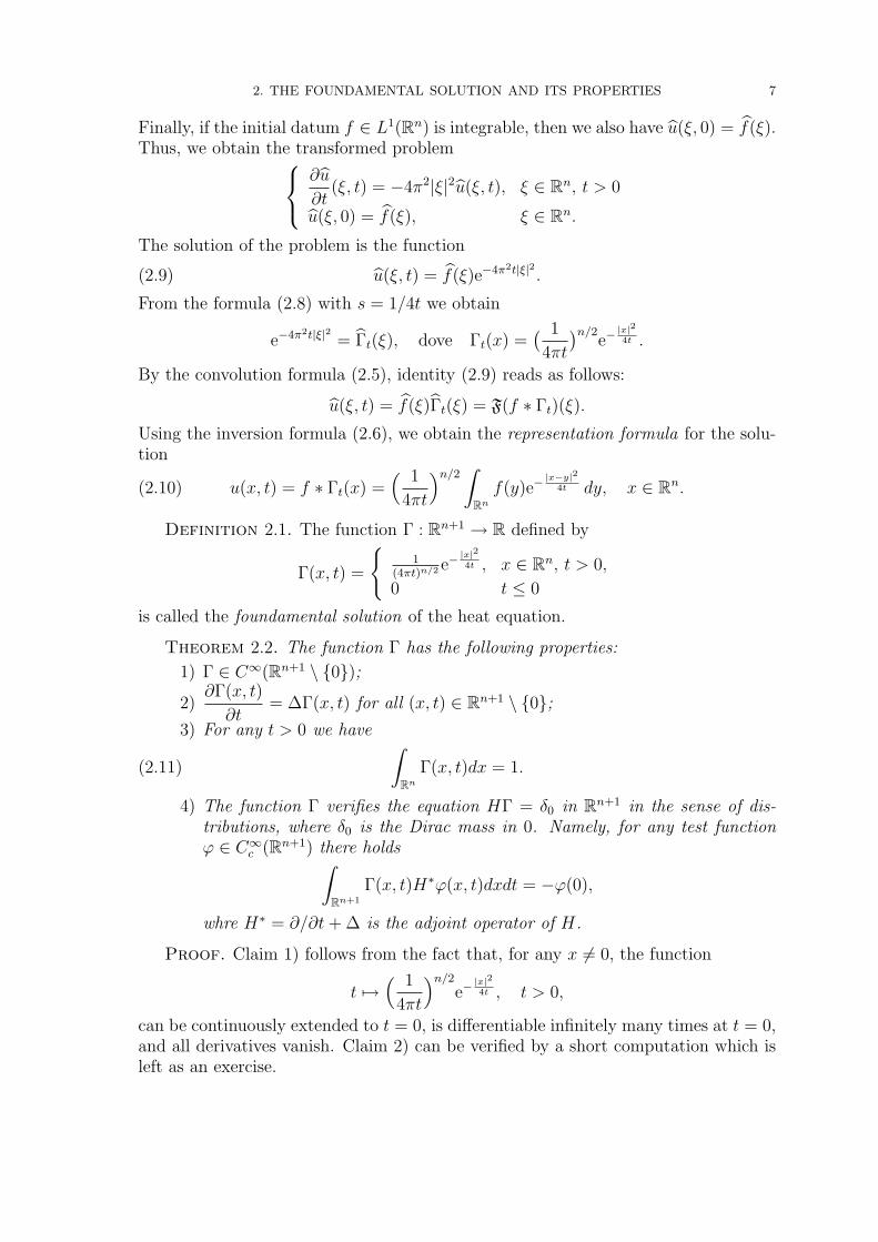
Finally, if the initial datum f ∈ L1(Rn) is integrable, then we also have u(ξ, 0) = f(ξ).Thus, we obtain the transformed problem

∂u

∂t(ξ, t) = −4π2|ξ|2u(ξ, t), ξ ∈ Rn, t > 0

u(ξ, 0) = f(ξ), ξ ∈ Rn.

The solution of the problem is the function

(2.9) u(ξ, t) = f(ξ)e−4π2t|ξ|2 .

From the formula (2.8) with s = 1/4t we obtain

e−4π2t|ξ|2 = Γt(ξ), dove Γt(x) =( 1

4πt

)n/2e−|x|24t .

By the convolution formula (2.5), identity (2.9) reads as follows:

u(ξ, t) = f(ξ)Γt(ξ) = F(f ∗ Γt)(ξ).

Using the inversion formula (2.6), we obtain the representation formula for the solu-tion

(2.10) u(x, t) = f ∗ Γt(x) =( 1

4πt

)n/2 ∫Rnf(y)e−

|x−y|24t dy, x ∈ Rn.

Definition 2.1. The function Γ : Rn+1 → R defined by

Γ(x, t) =

1

(4πt)n/2e−|x|24t , x ∈ Rn, t > 0,

0 t ≤ 0

is called the foundamental solution of the heat equation.

Theorem 2.2. The function Γ has the following properties:

1) Γ ∈ C∞(Rn+1 \ 0);

2)∂Γ(x, t)

∂t= ∆Γ(x, t) for all (x, t) ∈ Rn+1 \ 0;

3) For any t > 0 we have

(2.11)

∫Rn

Γ(x, t)dx = 1.

4) The function Γ verifies the equation HΓ = δ0 in Rn+1 in the sense of dis-tributions, where δ0 is the Dirac mass in 0. Namely, for any test functionϕ ∈ C∞c (Rn+1) there holds∫

Rn+1

Γ(x, t)H∗ϕ(x, t)dxdt = −ϕ(0),

whre H∗ = ∂/∂t+ ∆ is the adjoint operator of H.

Proof. Claim 1) follows from the fact that, for any x 6= 0, the function

t 7→( 1

4πt

)n/2e−|x|24t , t > 0,

can be continuously extended to t = 0, is differentiable infinitely many times at t = 0,and all derivatives vanish. Claim 2) can be verified by a short computation which isleft as an exercise.

8 1. HEAT EQUATION

Identity (2.11) follows from the well known formula∫ +∞

−∞e−s

2

ds =√π

and from Fubini-Tonelli theorem. In fact, we have:∫Rn

( 1

4πt

)n/2e−|x|24t dx =

( 1

4πt

)n/2 n∏i=1

∫ +∞

−∞e−

x2i4t dxi =

1

πn/2

n∏i=1

∫ +∞

−∞e−x

2i dxi = 1.

We prove Claim 4). For ΓH∗ϕ ∈ L1(Rn+1), by dominated convergence we have:∫Rn+1

Γ(x, t)H∗ϕ(x, t)dxdt =

∫ ∞0

∫Rn

Γ(x, t)H∗ϕ(x, t)dx dt

= limε↓0

∫ ∞ε

∫Rn

Γ(x, t)H∗ϕ(x, t)dx dt.

For any fixed t > 0, by an integration by parts we obtain∫Rn

Γ(x, t)∆ϕ(x, t)dx =

∫Rn

∆Γ(x, t)ϕ(x, t)dx.

There is no boundary contribution, because ϕ has compact support. Moreover, wehave ∫ ∞

ε

Γ(x, t)∂ϕ(x, t)

∂tdt = −

∫ ∞ε

∂Γ(x, t)

∂tϕ(x, t)dt− Γ(x, ε)ϕ(x, ε).

Summing up and using HΓ = 0, that holds on the set where t > 0, we obtain∫ ∞ε

∫Rn

Γ(x, t)H∗ϕ(x, t)dx dt =

∫ ∞ε

∫RnHΓ(x, t)ϕ(x, t)dx dt−

∫Rn

Γ(x, ε)ϕ(x, ε)dx

= −∫

RnΓ(x, ε)ϕ(x, ε)dx

= −∫

RnΓ(ξ, 1)ϕ(2

√εξ, ε)dξ.

Taking the limit as ε ↓ 0, by dominated convergence we prove the claim.

2.3. Cauchy Problem: existence of solutions.

Theorem 2.3. Let f ∈ C(Rn) ∩ L∞(Rn). The function u defined by the repre-sentation formula (2.10) solves the Cauchy Problem (1.1), and namely:

1) u ∈ C∞(Rn × (0,∞)) and ut(x, t) = ∆u(x, t) for all x ∈ Rn and t > 0;2) For any x0 ∈ Rn there holds

limx→x0,t↓0

u(x, t) = f(x0),

with uniform convergence for x0 belonging to a compact set;3) Moreover, ‖u(·, t)‖∞ ≤ ‖f‖∞ for all t > 0.

Proof. Claim 1) follows from the fact that we can take partial derivatives of anyorder in x and t into the integral in the representation formula (2.10). We prove, forinstance, that for any x ∈ Rn and for any t > 0 there holds

∂

∂t

∫Rnf(y)e−

|x−y|24t dy =

∫Rnf(y)

∂

∂te−|x−y|2

4t dy.

2. THE FOUNDAMENTAL SOLUTION AND ITS PROPERTIES 9

By the Corollary to the Dominated Convergence Theorem, it suffices to show thatfor any 0 < t0 ≤ T < ∞ there exists a function g ∈ L1(Rn), in variable y, such that(for fixed x ∈ Rn and) for any t ∈ [t0, T ] we have

|x− y|2

4t2e−|x−y|2

4t ≤ g(y), for all y ∈ Rn.

This holds with the choice

g(y) =|x− y|2

4t20e−|x−y|2

4T .

The case of derivatives in the variables x and the case of higher order derivatives isanalogous and is left as an exercise.

By the previous argument, it follows that, for t > 0, we can take the heat operatorinto the integral:

ut(x, t)−∆u(x, t) =

∫Rnf(y)

( ∂∂t−∆x

)Γ(x− y, t)dy

=

∫Rnf(y)

Γt(x− y, t)−∆Γ(x− y, t)

dy = 0.

Thus, u solves the heat equation for positive times.We prove claim 2). Let K ⊂ Rn be a compact set and let x0 ∈ K. We may rewrite

the representation formula (2.10) in the following way:

u(x, t) =1

πn/2

∫Rn

Γ(ξ, 1/4)f(2√tξ + x)dξ, x ∈ Rn, t > 0.

Hence, we have

|u(x, t)− f(x0)| ≤ 1

πn/2

∫Rn

Γ(ξ, 1/4)|f(2√tξ + x)− f(x0)|dξ.

Fix now ε > 0 and choose R > 0 such that

1

πn/2

∫|ξ|>R

Γ(ξ, 1/4)dξ ≤ ε.

As f is uniformly continuous on compact sets, there exists a δ > 0 such that for all|ξ| ≤ R we have

|x− x0| < δ and 0 < t < δ ⇒ |f(2√tξ − x)− f(x0)| < ε.

The choice of δ is uniform in x0 ∈ K. After all, we get

|u(x, t)− f(x0)| ≤ 1

πn/2

∫|ξ|≤R

Γ(ξ, 1/4)|f(2√tξ + x)− f(x0)|dξ

+1

πn/2

∫|ξ|>R

Γ(ξ, 1/4)|f(2√tξ + x)− f(x0)|dξ

≤ ε+ 2‖f‖∞ε.

This proves claim 2). Claim 3) follows directly from the representation formula.

10 1. HEAT EQUATION

2.4. Tychonov’s counterexample. In general, the solution of the Cauchy Pro-blem

(2.12)

ut(x, t) = ∆u(x, t), x ∈ Rn, t > 0,u(x, 0) = f(x), x ∈ Rn,

even with f ∈ C(Rn)∩L∞(Rn), is not unique in the class of functions C(Rn×[0,∞))∩C∞(Rn ∩ (0,∞)).

In dimension n = 1, let us consider the problem

(2.13)

ut(x, t) = uxx(x, t), x ∈ R, t > 0,u(x, 0) = 0, x ∈ R.

The function u = 0 is a solution. We construct a second solution that is not identicallyzero.

Let ϕ : C→ C be the function

ϕ(z) =

e−1/z2 , if z 6= 0,0, if z = 0.

The function ϕ is holomorphic in C\0. Moreover, the function t 7→ ϕ(t) with t ∈ Ris of class C∞(R) and ϕ(n)(0) = 0 for all n ∈ N. Let us consider the series of functions

u(x, t) =∞∑n=0

ϕ(n)(t)x2n

(2n)!, t ≥ 0, x ∈ R.

We shall prove the following facts:

1) The sum defining u and the series of the derivatives of any order convergeuniformly on any set of the form [−R,R]× [T,∞) with R, T > 0;

2) u is a continuous function up to the boundary in the halfspace t ≥ 0.

From 2) it follows that u attains the initial datum 0 at the time t = 0. By 1), we caninterchange sum and partial derivatives. Then we can compute

uxx(x, t) =∞∑n=1

ϕ(n)(t)x2n−2

(2n− 2)!=

∞∑m=0

ϕ(m+1)(t)x2m

(2m)!

=∂

∂t

∞∑m=0

ϕ(m)(t)x2m

(2m)!= ut(x, t).

Let us prove claim 1). For fixed t > 0, by the Cauchy formula for holomorphicfunctions we obtain

ϕ(n)(t) =n!

2πi

∫|z−t|=t/2

ϕ(z)

(z − t)n+1dz.

On the circle |z − t| = t/2, we have |ϕ(z)| ≤ e−Re(1/z2) ≤ e−4/t2 and thus

|ϕ(n)(t)| ≤ n!

2π

∫ 2π

0

e−4/t2

(t/2)n+1

t

2dϑ = n!2n

e−4/t2

tn.

We shall use the following inequality, that can be proved by induction:

n!2n

(2n)!≤ 1

n!.

2. THE FOUNDAMENTAL SOLUTION AND ITS PROPERTIES 11

Thus we get:

|u(x, t)| ≤∞∑n=0

|ϕ(n)(t)| |x|2n

(2n)!≤

∞∑n=0

n!2ne−4/t2

tn|x|2n

(2n)!

≤ e−4/t2∞∑n=0

1

n!

( |x|2t

)n= e−4/t2+|x|2/t,

where the last sum converges uniformly for t ≥ T > 0 and |x| ≤ R < ∞. ByWeierstrass’ criterion, the sum defining u converges uniformly on the same set. Inparticular, by comparison we find

limt→0

e−4/t2+|x|2/t = 0 ⇒ limt→0|u(x, t)| = 0

with uniform convergence for |x| ≤ R. This proves claim 2).The study of convergence of the series of derivatives is analogous and is left as an

exercise to the reader.

2.5. Nonhomogeneous problem. Let us consider the nonhomogeneous Cauchyproblem

(2.14)

ut(x, t)−∆u(x, t) = f(x, t), x ∈ Rn, t > 0,u(x, 0) = 0, x ∈ Rn,

where f : Rn × (0,∞) → R is a suitable function. We discuss the regularity of flater. A candidate solution of the problem can be obtained on using the “Duhamel’sPrinciple”. Fix s > 0 and assume there exists a (the) solution v(·; s) of the CauchyProblem

(2.15)

vt(x, t; s) = ∆v(x, t; s), x ∈ Rn, t > s,v(x, s; s) = f(x, s), x ∈ Rn.

On integrating the solutions v(x, t; s) for s ∈ (0, t) we obtain the function

(2.16) u(x, t) =

∫ t

0

v(x, t; s)ds.

When we formally insert t = 0 into this identity, we get u(x, 0) = 0. If we formallydifferentiate the identity – taking derivatives into the integral is a idelicate issue, here,– we obtain

ut(x, t) = v(x, t; t) +

∫ t

0

vt(x, t; s)ds e ∆u(x, t) =

∫ t

0

∆v(x, t; s)ds,

and thus ut(x, t) − ∆u(x, t) = v(x, t; t) = f(x, t). If the previous computations areallowed, the function u is a solution to the problem (2.14).

Inserting the representation formula (2.10) for the solutions v(x, t; s) into (2.16),we get the representation formula for the solution u

(2.17) u(x, t) =

∫ t

0

∫Rn

Γ(x− y, t− s)f(y, s)dy ds, x ∈ Rn, t > 0.

In order the make rigorous the previuous argument, we need estimates for thesolution to the Cauchy problem near time t = 0.

12 1. HEAT EQUATION

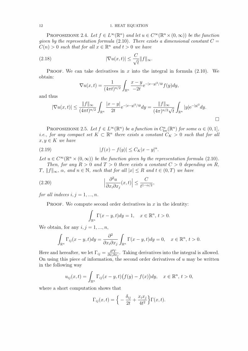
Proposizione 2.4. Let f ∈ L∞(Rn) and let u ∈ C∞(Rn× (0,∞)) be the functiongiven by the representation formula (2.10). There exists a dimensional constant C =C(n) > 0 such that for all x ∈ Rn and t > 0 we have

(2.18) |∇u(x, t)| ≤ C√t‖f‖∞.

Proof. We can take derivatives in x into the integral in formula (2.10). Weobtain:

∇u(x, t) =1

(4πt)n/2

∫Rn

x− y−2t

e−|x−y|2/4tf(y)dy,

and thus

|∇u(x, t)| ≤ ‖f‖∞(4πt)n/2

∫Rn

|x− y|2t

e−|x−y|2/4tdy =

‖f‖∞(4π)n/2

√t

∫Rn|y|e−|y|2dy.

Proposizione 2.5. Let f ∈ L∞(Rn) be a function in Cαloc(Rn) for some α ∈ (0, 1],

i.e., for any compact set K ⊂ Rn there exists a constant CK > 0 such that for allx, y ∈ K we have

(2.19) |f(x)− f(y)| ≤ CK |x− y|α.

Let u ∈ C∞(Rn × (0,∞)) be the function given by the representation formula (2.10).Then, for any R > 0 and T > 0 there exists a constant C > 0 depending on R,

T , ‖f‖∞, α, and n ∈ N, such that for all |x| ≤ R and t ∈ (0, T ) we have

(2.20)∣∣∣ ∂2u

∂xi∂xj(x, t)

∣∣∣ ≤ C

t1−α/2,

for all indeces i, j = 1, ..., n.

Proof. We compute second order derivatives in x in the identity:∫Rn

Γ(x− y, t)dy = 1, x ∈ Rn, t > 0.

We obtain, for any i, j = 1, ..., n,∫Rn

Γij(x− y, t)dy =∂2

∂xi∂xj

∫Rn

Γ(x− y, t)dy = 0, x ∈ Rn, t > 0.

Here and hereafter, we let Γij = ∂2Γ∂xi∂xj

. Taking derivatives into the integral is allowed.

On using this piece of information, the second order derivatives of u may be writtenin the following way

uij(x, t) =

∫Rn

Γij(x− y, t)(f(y)− f(x)

)dy, x ∈ Rn, t > 0,

where a short computation shows that

Γij(x, t) =− δij

2t+xixj4t2

Γ(x, t).

2. THE FOUNDAMENTAL SOLUTION AND ITS PROPERTIES 13

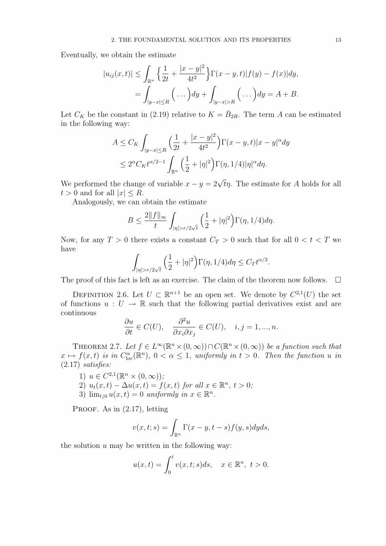
Eventually, we obtain the estimate

|uij(x, t)| ≤∫

Rn

1

2t+|x− y|2

4t2

Γ(x− y, t)|f(y)− f(x)|dy,

=

∫|y−x|≤R

(. . .)dy +

∫|y−x|>R

(. . .)dy = A+B.

Let CK be the constant in (2.19) relative to K = B2R. The term A can be estimatedin the following way:

A ≤ CK

∫|y−x|≤R

( 1

2t+|x− y|2

4t2

)Γ(x− y, t)|x− y|αdy

≤ 2αCKtα/2−1

∫Rn

(1

2+ |η|2

)Γ(η, 1/4)|η|αdη.

We performed the change of variable x− y = 2√tη. The estimate for A holds for all

t > 0 and for all |x| ≤ R.Analogously, we can obtain the estimate

B ≤ 2‖f‖∞t

∫|η|>r/2

√t

(1

2+ |η|2

)Γ(η, 1/4)dη.

Now, for any T > 0 there exists a constant CT > 0 such that for all 0 < t < T wehave ∫

|η|>r/2√t

(1

2+ |η|2

)Γ(η, 1/4)dη ≤ CT t

α/2.

The proof of this fact is left as an exercise. The claim of the theorem now follows.

Definition 2.6. Let U ⊂ Rn+1 be an open set. We denote by C2,1(U) the setof functions u : U → R such that the following partial derivatives exist and arecontinuous

∂u

∂t∈ C(U),

∂2u

∂xi∂xj∈ C(U), i, j = 1, ..., n.

Theorem 2.7. Let f ∈ L∞(Rn× (0,∞))∩C(Rn× (0,∞)) be a function such thatx 7→ f(x, t) is in Cα

loc(Rn), 0 < α ≤ 1, uniformly in t > 0. Then the function u in(2.17) satisfies:

1) u ∈ C2,1(Rn × (0,∞));2) ut(x, t)−∆u(x, t) = f(x, t) for all x ∈ Rn, t > 0;3) limt↓0 u(x, t) = 0 uniformly in x ∈ Rn.

Proof. As in (2.17), letting

v(x, t; s) =

∫Rn

Γ(x− y, t− s)f(y, s)dyds,

the solution u may be written in the following way:

u(x, t) =

∫ t

0

v(x, t; s)ds, x ∈ Rn, t > 0.

14 1. HEAT EQUATION

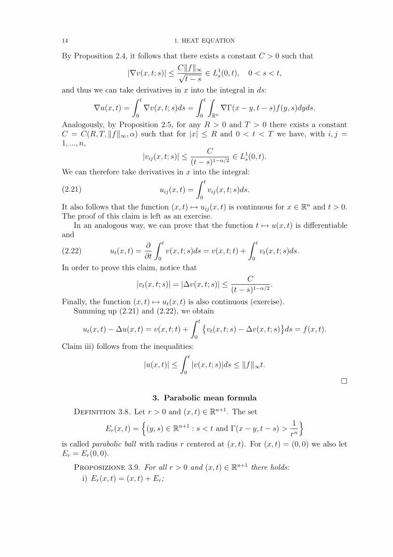
By Proposition 2.4, it follows that there exists a constant C > 0 such that

|∇v(x, t; s)| ≤ C‖f‖∞√t− s

∈ L1s(0, t), 0 < s < t,

and thus we can take derivatives in x into the integral in ds:

∇u(x, t) =

∫ t

0

∇v(x, t; s)ds =

∫ t

0

∫Rn∇Γ(x− y, t− s)f(y, s)dyds.

Analogously, by Proposition 2.5, for any R > 0 and T > 0 there exists a constantC = C(R, T, ‖f‖∞, α) such that for |x| ≤ R and 0 < t < T we have, with i, j =1, ..., n,

|vij(x, t; s)| ≤C

(t− s)1−α/2 ∈ L1s(0, t).

We can therefore take derivatives in x into the integral:

uij(x, t) =

∫ t

0

vij(x, t; s)ds.(2.21)

It also follows that the function (x, t) 7→ uij(x, t) is continuous for x ∈ Rn and t > 0.The proof of this claim is left as an exercise.

In an analogous way, we can prove that the function t 7→ u(x, t) is differentiableand

(2.22) ut(x, t) =∂

∂t

∫ t

0

v(x, t; s)ds = v(x, t; t) +

∫ t

0

vt(x, t; s)ds.

In order to prove this claim, notice that

|vt(x, t; s)| = |∆v(x, t; s)| ≤ C

(t− s)1−α/2 .

Finally, the function (x, t) 7→ ut(x, t) is also continuous (exercise).Summing up (2.21) and (2.22), we obtain

ut(x, t)−∆u(x, t) = v(x, t; t) +

∫ t

0

vt(x, t; s)−∆v(x, t; s)

ds = f(x, t).

Claim iii) follows from the inequalities:

|u(x, t)| ≤∫ t

0

|v(x, t; s)|ds ≤ ‖f‖∞t.

3. Parabolic mean formula

Definition 3.8. Let r > 0 and (x, t) ∈ Rn+1. The set

Er(x, t) =

(y, s) ∈ Rn+1 : s < t and Γ(x− y, t− s) > 1

rn

is called parabolic ball with radius r centered at (x, t). For (x, t) = (0, 0) we also letEr = Er(0, 0).

Proposizione 3.9. For all r > 0 and (x, t) ∈ Rn+1 there holds:

i) Er(x, t) = (x, t) + Er;

3. PARABOLIC MEAN FORMULA 15

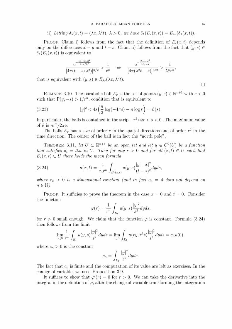
ii) Letting δλ(x, t) = (λx, λ2t), λ > 0, we have δλ(Er(x, t)) = Eλr(δλ(x, t)).

Proof. Claim i) follows from the fact that the definition of Er(x, t) dependsonly on the differences x − y and t − s. Claim ii) follows from the fact that (y, s) ∈δλ(Er(x, t)) is equivalent to

e− |x−y/λ|

2

t−s/λ2

[4π(t− s/λ2)]n/2>

1

rn⇔ e

− |λx−y|2

λ2t−s

[4π(λ2t− s)]n/2>

1

λnrn,

that is equivalent with (y, s) ∈ Eλr(λx, λ2t).

Remark 3.10. The parabolic ball Er is the set of points (y, s) ∈ Rn+1 with s < 0such that Γ(y,−s) > 1/rn, condition that is equivalent to

(3.23) |y|2 < 4s(n

2log(−4πs)− n log r

)= ϑ(s).

In particular, the balls is contained in the strip −r2/4π < s < 0. The maximum valueof ϑ is nr2/2πe.

The balls Er has a size of order r in the spatial directions and of order r2 in thetime direction. The center of the ball is in fact the “north pole”.

Theorem 3.11. let U ⊂ Rn+1 be an open set and let u ∈ C2(U) be a functionthat satisfies ut = ∆u in U . Then for any r > 0 and for all (x, t) ∈ U such thatEr(x, t) ⊂ U there holds the mean formula

(3.24) u(x, t) =1

cnrn

∫Er(x,t)

u(y, s)|y − x|2

(t− s)2dyds,

where cn > 0 is a dimensional constant (and in fact cn = 4 does not depend onn ∈ N).

Proof. It sufficies to prove the theorem in the case x = 0 and t = 0. Considerthe function

ϕ(r) =1

rn

∫Er

u(y, s)|y|2

s2dyds,

for r > 0 small enough. We claim that the function ϕ is constant. Formula (3.24)then follows from the limit

limr↓0

1

rn

∫Er

u(y, s)|y|2

s2dyds = lim

r↓0

∫E1

u(ry, r2s)|y|2

s2dyds = cnu(0),

where cn > 0 is the constant

cn =

∫E1

|y|2

s2dyds.

The fact that cn is finite and the computation of its value are left as exercises. In thechange of variable, we used Proposition 3.9.

It suffices to show that ϕ′(r) = 0 for r > 0. We can take the derivative into theintegral in the definition of ϕ, after the change of variable transforming the integration

16 1. HEAT EQUATION

domain into E1:

ϕ′(r) =

∫E1

y · ∇u(ry, r2s) + 2rsus(ry, r

2s) |y|2s2dyds

=1

rn+1

∫Er

y · ∇u(y, s) + 2sus(y, s)

|y|2s2dyds

=1

rn+1

∫Er

y · ∇u(y, s)|y|2

s2dyds+

1

rn+1

∫Er

2us(y, s)|y|2

sdyds

=1

rn+1

(A+B

).

Consider the function

ψ(y, s) =|y|2

4s− n

2log(−4πs) + n log r.

The definition of ψ is suggested by condition (3.23) that characterizes the parabolicball Er. The function satisfies ψ = 0 on ∂Er and, moreover,

(3.25) ∇ψ(y, s) =y

2s.

We use the last identity to transform B in the following way:

B =

∫Er

2us(y, s)|y|2

sdyds = 4

∫Er

us(y, s)y · ∇ψ(y, s)dyds

= −4

∫Er

ψ(y, s)div(us(y, s)y)dyds

= −4

∫Er

ψ(y, s)y · ∇us(y, s) + nus(y, s)

dyds.

We used the divergence theorem (integration by parts) in the variables y for fixeds (and, implicitly, also Fubini-Tonelli theorem). Now we integrate by parts in s forfixed y in the first term, and we use the differential equation us = ∆u in the secondone. We get

B = 4

∫Er

ψs(y, s)y · ∇u(y, s)− nψ(y, s)∆u(y, s)

dyds

= 4

∫Er

− |y|

2

4s2− n

2s

y · ∇u(y, s)dyds+ 4n

∫Er

∇ψ(y, s) · ∇u(y, s)dyds

= −∫Er

|y|2

s2y · ∇u(y, s)dyds = −A.

We used again the divergence theorem and the properties of ψ.We eventually obtain A+B = 0 identically in r > 0 and the theorem is proved.

4. Parabolic maximum principles

Let Ω ⊂ Rn be an open set and T > 0. We denote by ΩT = Ω×(0, T ) the cylinderof height T over Ω. With abuse of notation, we define the parabolic boundary of ΩT

as the set ∂ΩT ⊂ Rn+1 defined in the following way

∂ΩT = ∂Ω× [0, T ] ∪ Ω× 0.

4. PARABOLIC MAXIMUM PRINCIPLES 17

Theorem 4.12 (Weak maximum principle). Let Ω ⊂ Rn be a bounded open setand let u ∈ C2(ΩT ) ∩ C(ΩT ) be a solution of the equation ut −∆u = 0 in ΩT . Thenwe have

maxΩT|u| = max

∂ΩT|u|.

The weak maximum principle is a corollary of the strong maximum principle. Wepostpone the proof.

Theorem 4.13 (Strong maximum principle). Let Ω ⊂ Rn be a connected open setand let u ∈ C2(ΩT ) be a solution to the differential equation ut −∆u = 0 in ΩT . Ifthere is a point (x0, t0) ∈ ΩT such that

|u(x0, t0)| = max(x,t)∈ΩT

|u(x, t)|

then we have u(x, t) = u(x0, t0) for all (x, t) ∈ Ω× (0, t0].

Proof. Let (x0, t0) ∈ ΩT be a point such that

u(x0, t0) = M := max(x,t)∈ΩT

u(x, t).

Let (x, t) ∈ ΩT be any point such that t < t0 and such that the line segment Sconnecting (x0, t0) to (x, t), i.e.,

S =

(xτ , tτ ) = (1− τ)(x0, t0) + τ(x, t) ∈ Rn+1 : 0 ≤ τ ≤ 1,

is entirely contained in ΩT . Let

A =τ ∈ [0, 1] : u(xτ , tτ ) = M

.

We have A 6= ∅ because 0 ∈ A. We shall prove that if τ ∈ A then also τ + δ ∈ A forall 0 < δ < δ0, for some δ0 > 0. Indeed, there exists r > 0 such that Er(xτ , tτ ) ⊂ ΩT ,because ΩT is open and thus, by the parabolic mean formula, we have

M = u(xτ , tτ ) =1

4rn

∫Er(xτ ,tτ )

u(y, s)|y − xτ |2

(s− tτ )2dyds

≤ M

4rn

∫Er(xτ ,tτ )

|y − xτ |2

(s− tτ )2dyds = M.

It follows that u = M in Er(xτ , tτ ) and the existence of δ > 0 is implied by the“shape” of parabolic balls. From the previous argument it follows that A = [0, 1] andthus u = M on S.

Let (x, t) ∈ ΩT be any point such that 0 < t < t0. As Ω is a connectedopen set, then it is pathwise connected by polygonal arcs: there exist m + 1 pointsx0, x1, ..., xm = x contained Ω such that each segment [xi−1, xi], i = 1, ...,m, is con-tained in Ω. Choose times t0 > t1 > ... > tm = t. A successive application of the previ-ous argument shows that u = M on each segment Si =

(1−τ)(xi−1, ti−1)+τ(xi, ti) ∈

ΩT : 0 ≤ τ ≤ 1

and thus u(x, t) = M . By continuity, the claim holds also fort = t0.

Proof of Theorem 4.12. We prove for instance that

M = maxΩT

u = max∂ΩT

u.

18 1. HEAT EQUATION

Notice that the maximum on the left hand side is attained, beacause u is continuousin ΩT , that is a compact set. Then there exists (x0, t0) ∈ ΩT such that u(x0, t0) = M .

If (x0, t0) ∈ ∂ΩT the proof is finished. Let (x0, t0) ∈ Ω×(0, T ]. Let Ωx0 ⊂ Ω denotethe connected component of Ω containing x0. From the strong maximum principle itfollows that u = M on Ωx0 × (0, t0]. This holds also in the case t0 = T . Eventually,u attaines the maximum (also) on the parabolic boundary ∂ΩT .

The weak maximum principle implies the uniqueness of the solution of the para-bolic Dirichlet problem on a bounded domain with initial and boundary conditions.

Theorem 4.14 (Uniqueness for the Dirichlet problem). Let Ω ⊂ Rn be a boundedset, T > 0, f ∈ C(ΩT ) and g ∈ C(∂ΩT ). Then the problem

(4.26)

ut −∆u = f, in ΩT ,u = g, su ∂ΩT ,

has at most one solution u ∈ C2(ΩT ) ∩ C(ΩT ).

Proof. Indeed, if u, v are solutions then the function w = u − v satisfies w = 0on ∂ΩT and wt −∆w = 0 in ΩT . From the weak maximum principle, it follows thatmaxΩT |w| = max∂Ωt |w| = 0 and thus u = v.

The uniqueness for the Cauchy problem on Rn requires a global version of themaximum principle.

Theorem 4.15. Let f ∈ C(Rn) and let u ∈ C2(Rn × (0, T )) ∩ C(Rn × [0, T ]) bea solution of the Cauchy problem

(4.27)

ut −∆u = 0, in Rn × (0, T ),u = f, su Rn

that satisfies for some constants A, b > 0

(4.28) |u(x, t)| ≤ Aeb|x|2

, x ∈ Rn, t ∈ [0, T ].

Then we have

(4.29) supx∈Rn, t∈[0,T ]

|u(x, t)| ≤ supx∈Rn|f(x)|.

Proof. We prove, for instance, that u(x, t) ≤ supRn f for x ∈ Rn and t ∈ [0, T ].Assume that there also holds 4bT < 1. This assumption will be removed at the endof the proof. Then there exists ε > 0 such that 4b(T + ε) < 1 and thus 1

4(T+ε)= b+ γ

for some γ > 0. Let δ > 0 be a positive parameter and consider the function

v(x, t) = u(x, t)− δ

(T + ε− t)n/2e

|x|24(T+ε−t) , x ∈ Rn, t ∈ [0, T ].

An explicit computation, that is omitted, shows that vt = ∆v. Moreover, from (4.28)it follows that for x ∈ Rn and t ∈ [0, T ] we have

v(x, t) ≤ Aeb|x|2 − δ

(T + ε)n/2e|x|2

4(T+ε) = Aeb|x|2 − δ

(T + ε)n/2e(b+γ)|x|2 .

As δ > 0, there exists R > 0 such that for |x| ≥ R and for all t ∈ [0, T ] we have

v(x, t) ≤ supx∈Rn

f(x).

5. REGULARITY OF LOCAL SOLUTIONS AND CAUCHY ESTIMATES 19

On the other hand, letting Ω = |x| < R, by the weak maximum principle we have

max(x,t)∈ΩT

v(x, t) = max(x,t)∈∂ΩT

v(x, t) ≤ supx∈Rn

f(x).

After all, we obtain

u(x, t)− δ

(T + ε− t)n/2e

|x|24(T+ε−t) = v(x, t) ≤ sup

x∈Rnf(x), x ∈ Rn, t ∈ [0, T ],

and letting δ ↓ 0 we obtain the claim.The restriction 4bT < 1 can be removed on dividing the interval [0, T ] into subin-

tervals [0, T1], [T1, 2T1], [(k−1)T1, kT1] with kT1 = T and 4bT1 < 1, and then applyingthe previous argument to each subinterval.

Theorem 4.16 (Uniqueness for the Cauchy problem). Let T > 0, f ∈ C(Rn ×[0, T ]) and g ∈ C(Rn). Then the Cauchy problem

(4.30)

ut −∆u = f, in Rn × (0, T ),u(x, 0) = g(x), for x ∈ Rn,

has at most one solution u ∈ C2(Rn × (0, T )) ∩ C(Rn × [0, T ]) within the class offunctions that satisfies the growth condition

(4.31) |u(x, t)| ≤ Aeb|x|2

, x ∈ Rn, t ∈ [0, T ],

for some constants A, b > 0.

The proof is an elementary exercise.

5. Regularity of local solutions and Cauchy estimates

Let us define the parabolic cylinder centered at (x, t) ∈ Rn+1 with radius r > 0 asthe set Cr(x, t) ⊂ Rn+1 defined in the following way

Cr(x, t) =

(y, s) ∈ Rn+1 : |y − x| < r, t− r2 < s < t.

In the sequel, we shall also let Cr = Cr(0, 0). The sets Cr(x, t) are a cylindricalversion of the parabolic balls Er(x, t).

Theorem 5.17. Let Ω ⊂ Rn be an open set, T > 0, and let u ∈ C2,1(ΩT ) be asolution to the equation ut −∆u = 0 in ΩT . Then there holds u ∈ C∞(ΩT ).

Proof. Let (x0, t0) ∈ ΩT be a fixed point and let us define the cylinders

C ′ = Cr(x0, t0), C ′′ = C2r(x0, t0), C ′′′ = C3r(x0, t0).

We fix the radius r > 0 small enough in such a way that C ′′′ ⊂ ΩT .Let ζ ∈ C∞(Rn+1) be a cutt-off function with the following properties: ζ = 1

on C ′′ and ζ = 0 on Rn × [0, t0] \ C ′′′. The function v = ζu satisfies the followingdifferential equation

vt −∆v = ζ(ut −∆u) + uζt − 2∇ζ · ∇u− u∆ζ = uζt − 2∇ζ · ∇u− u∆ζ = f.

20 1. HEAT EQUATION

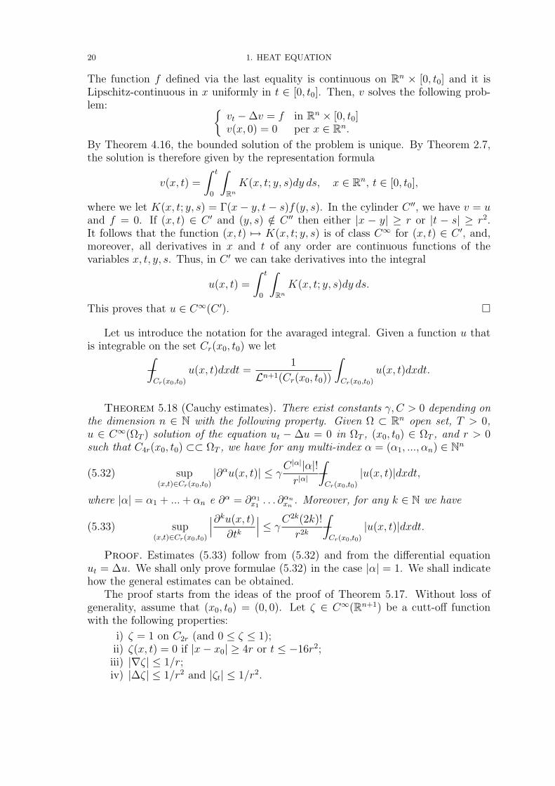
The function f defined via the last equality is continuous on Rn × [0, t0] and it isLipschitz-continuous in x uniformly in t ∈ [0, t0]. Then, v solves the following prob-lem:

vt −∆v = f in Rn × [0, t0]v(x, 0) = 0 per x ∈ Rn.

By Theorem 4.16, the bounded solution of the problem is unique. By Theorem 2.7,the solution is therefore given by the representation formula

v(x, t) =

∫ t

0

∫RnK(x, t; y, s)dy ds, x ∈ Rn, t ∈ [0, t0],

where we let K(x, t; y, s) = Γ(x− y, t− s)f(y, s). In the cylinder C ′′, we have v = uand f = 0. If (x, t) ∈ C ′ and (y, s) /∈ C ′′ then either |x − y| ≥ r or |t − s| ≥ r2.It follows that the function (x, t) 7→ K(x, t; y, s) is of class C∞ for (x, t) ∈ C ′, and,moreover, all derivatives in x and t of any order are continuous functions of thevariables x, t, y, s. Thus, in C ′ we can take derivatives into the integral

u(x, t) =

∫ t

0

∫RnK(x, t; y, s)dy ds.

This proves that u ∈ C∞(C ′).

Let us introduce the notation for the avaraged integral. Given a function u thatis integrable on the set Cr(x0, t0) we let∫

Cr(x0,t0)

u(x, t)dxdt =1

Ln+1(Cr(x0, t0))

∫Cr(x0,t0)

u(x, t)dxdt.

Theorem 5.18 (Cauchy estimates). There exist constants γ, C > 0 depending onthe dimension n ∈ N with the following property. Given Ω ⊂ Rn open set, T > 0,u ∈ C∞(ΩT ) solution of the equation ut − ∆u = 0 in ΩT , (x0, t0) ∈ ΩT , and r > 0such that C4r(x0, t0) ⊂⊂ ΩT , we have for any multi-index α = (α1, ..., αn) ∈ Nn

(5.32) sup(x,t)∈Cr(x0,t0)

|∂αu(x, t)| ≤ γC |α||α|!r|α|

∫Cr(x0,t0)

|u(x, t)|dxdt,

where |α| = α1 + ...+ αn e ∂α = ∂α1x1. . . ∂αnxn . Moreover, for any k ∈ N we have

(5.33) sup(x,t)∈Cr(x0,t0)

∣∣∣∂ku(x, t)

∂tk

∣∣∣ ≤ γC2k(2k)!

r2k

∫Cr(x0,t0)

|u(x, t)|dxdt.

Proof. Estimates (5.33) follow from (5.32) and from the differential equationut = ∆u. We shall only prove formulae (5.32) in the case |α| = 1. We shall indicatehow the general estimates can be obtained.

The proof starts from the ideas of the proof of Theorem 5.17. Without loss ofgenerality, assume that (x0, t0) = (0, 0). Let ζ ∈ C∞(Rn+1) be a cutt-off functionwith the following properties:

i) ζ = 1 on C2r (and 0 ≤ ζ ≤ 1);ii) ζ(x, t) = 0 if |x− x0| ≥ 4r or t ≤ −16r2;

iii) |∇ζ| ≤ 1/r;iv) |∆ζ| ≤ 1/r2 and |ζt| ≤ 1/r2.

5. REGULARITY OF LOCAL SOLUTIONS AND CAUCHY ESTIMATES 21

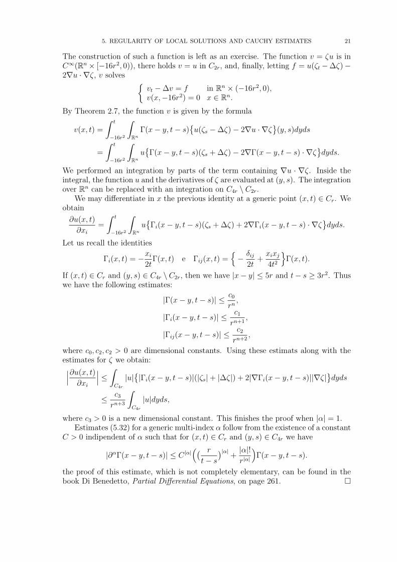
The construction of such a function is left as an exercise. The function v = ζu is inC∞(Rn × [−16r2, 0)), there holds v = u in C2r, and, finally, letting f = u(ζt −∆ζ)−2∇u · ∇ζ, v solves

vt −∆v = f in Rn × (−16r2, 0),v(x,−16r2) = 0 x ∈ Rn.

By Theorem 2.7, the function v is given by the formula

v(x, t) =

∫ t

−16r2

∫Rn

Γ(x− y, t− s)u(ζs −∆ζ)− 2∇u · ∇ζ

(y, s)dyds

=

∫ t

−16r2

∫Rnu

Γ(x− y, t− s)(ζs + ∆ζ)− 2∇Γ(x− y, t− s) · ∇ζdyds.

We performed an integration by parts of the term containing ∇u · ∇ζ. Inside theintegral, the function u and the derivatives of ζ are evaluated at (y, s). The integrationover Rn can be replaced with an integration on C4r \ C2r.

We may differentiate in x the previous identity at a generic point (x, t) ∈ Cr. Weobtain

∂u(x, t)

∂xi=

∫ t

−16r2

∫Rnu

Γi(x− y, t− s)(ζs + ∆ζ) + 2∇Γi(x− y, t− s) · ∇ζdyds.

Let us recall the identities

Γi(x, t) = −xi2t

Γ(x, t) e Γij(x, t) =− δij

2t+xixj4t2

Γ(x, t).

If (x, t) ∈ Cr and (y, s) ∈ C4r \C2r, then we have |x− y| ≤ 5r and t− s ≥ 3r2. Thuswe have the following estimates:

|Γ(x− y, t− s)| ≤ c0

rn,

|Γi(x− y, t− s)| ≤c1

rn+1,

|Γij(x− y, t− s)| ≤c2

rn+2,

where c0, c2, c2 > 0 are dimensional constants. Using these estimats along with theestimates for ζ we obtain:∣∣∣∂u(x, t)

∂xi

∣∣∣ ≤ ∫C4r

|u||Γi(x− y, t− s)|(|ζs|+ |∆ζ|) + 2|∇Γi(x− y, t− s)||∇ζ|

dyds

≤ c3

rn+3

∫C4r

|u|dyds,

where c3 > 0 is a new dimensional constant. This finishes the proof when |α| = 1.Estimates (5.32) for a generic multi-index α follow from the existence of a constant

C > 0 indipendent of α such that for (x, t) ∈ Cr and (y, s) ∈ C4r we have

|∂αΓ(x− y, t− s)| ≤ C |α|(( r

t− s)|α|

+|α|!r|α|

)Γ(x− y, t− s).

the proof of this estimate, which is not completely elementary, can be found in thebook Di Benedetto, Partial Differential Equations, on page 261.

22 1. HEAT EQUATION

6. Harnack inequality

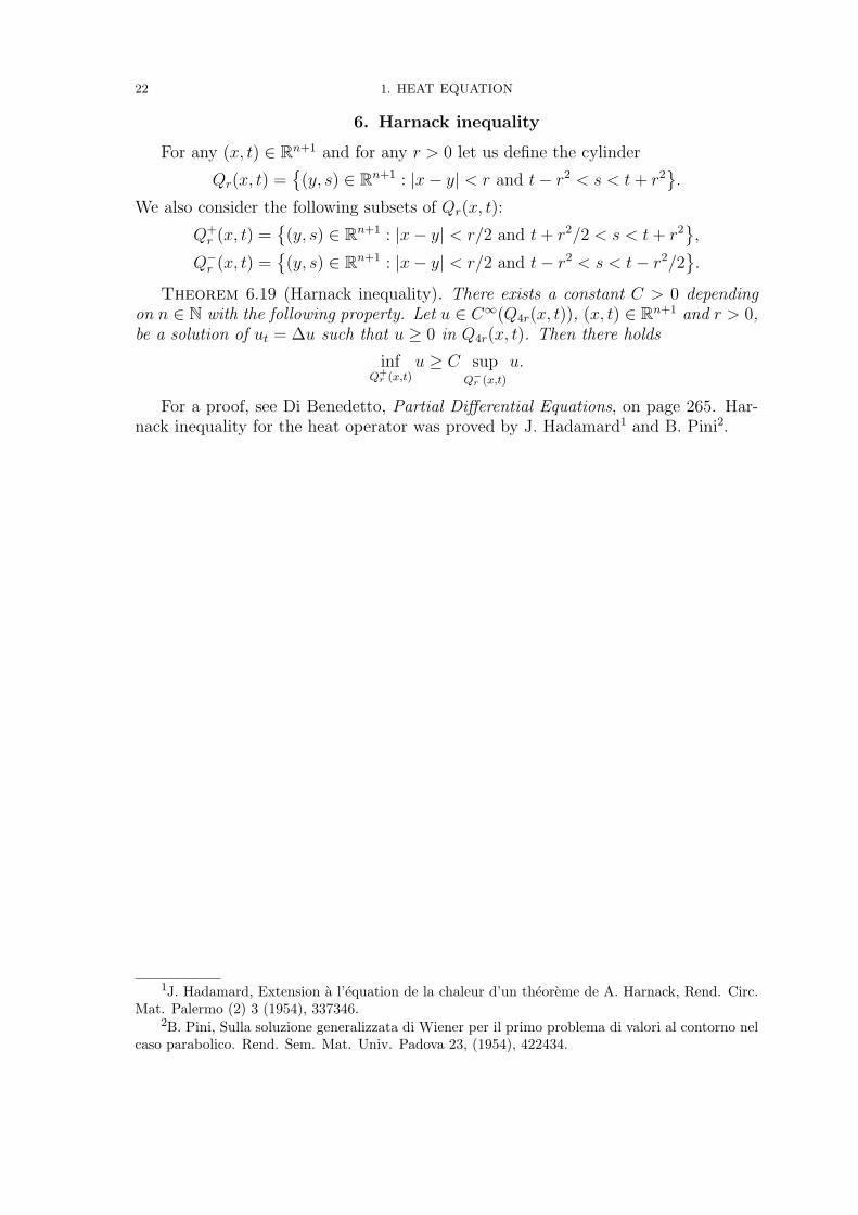
For any (x, t) ∈ Rn+1 and for any r > 0 let us define the cylinder

Qr(x, t) =

(y, s) ∈ Rn+1 : |x− y| < r and t− r2 < s < t+ r2.

We also consider the following subsets of Qr(x, t):

Q+r (x, t) =

(y, s) ∈ Rn+1 : |x− y| < r/2 and t+ r2/2 < s < t+ r2

,

Q−r (x, t) =

(y, s) ∈ Rn+1 : |x− y| < r/2 and t− r2 < s < t− r2/2.

Theorem 6.19 (Harnack inequality). There exists a constant C > 0 dependingon n ∈ N with the following property. Let u ∈ C∞(Q4r(x, t)), (x, t) ∈ Rn+1 and r > 0,be a solution of ut = ∆u such that u ≥ 0 in Q4r(x, t). Then there holds

infQ+r (x,t)

u ≥ C supQ−r (x,t)

u.

For a proof, see Di Benedetto, Partial Differential Equations, on page 265. Har-nack inequality for the heat operator was proved by J. Hadamard1 and B. Pini2.

1J. Hadamard, Extension a l’equation de la chaleur d’un theoreme de A. Harnack, Rend. Circ.Mat. Palermo (2) 3 (1954), 337346.

2B. Pini, Sulla soluzione generalizzata di Wiener per il primo problema di valori al contorno nelcaso parabolico. Rend. Sem. Mat. Univ. Padova 23, (1954), 422434.

CHAPTER 2

Maximum principles

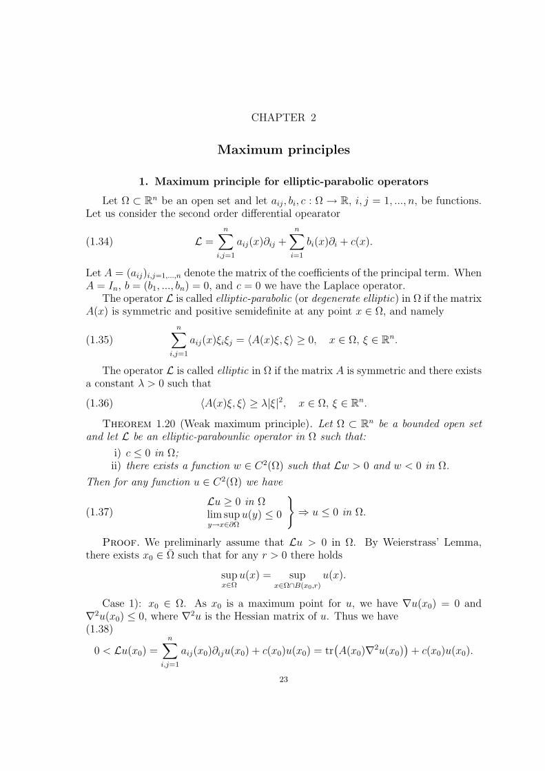
1. Maximum principle for elliptic-parabolic operators

Let Ω ⊂ Rn be an open set and let aij, bi, c : Ω → R, i, j = 1, ..., n, be functions.Let us consider the second order differential opearator

(1.34) L =n∑

i,j=1

aij(x)∂ij +n∑i=1

bi(x)∂i + c(x).

Let A = (aij)i,j=1,...,n denote the matrix of the coefficients of the principal term. WhenA = In, b = (b1, ..., bn) = 0, and c = 0 we have the Laplace operator.

The operator L is called elliptic-parabolic (or degenerate elliptic) in Ω if the matrixA(x) is symmetric and positive semidefinite at any point x ∈ Ω, and namely

(1.35)n∑

i,j=1

aij(x)ξiξj = 〈A(x)ξ, ξ〉 ≥ 0, x ∈ Ω, ξ ∈ Rn.

The operator L is called elliptic in Ω if the matrix A is symmetric and there existsa constant λ > 0 such that

(1.36) 〈A(x)ξ, ξ〉 ≥ λ|ξ|2, x ∈ Ω, ξ ∈ Rn.

Theorem 1.20 (Weak maximum principle). Let Ω ⊂ Rn be a bounded open setand let L be an elliptic-parabounlic operator in Ω such that:

i) c ≤ 0 in Ω;ii) there exists a function w ∈ C2(Ω) such that Lw > 0 and w < 0 in Ω.

Then for any function u ∈ C2(Ω) we have

(1.37)Lu ≥ 0 in Ωlim supy→x∈∂Ω

u(y) ≤ 0

⇒ u ≤ 0 in Ω.

Proof. We preliminarly assume that Lu > 0 in Ω. By Weierstrass’ Lemma,there exists x0 ∈ Ω such that for any r > 0 there holds

supx∈Ω

u(x) = supx∈Ω∩B(x0,r)

u(x).

Case 1): x0 ∈ Ω. As x0 is a maximum point for u, we have ∇u(x0) = 0 and∇2u(x0) ≤ 0, where ∇2u is the Hessian matrix of u. Thus we have(1.38)

0 < Lu(x0) =n∑

i,j=1

aij(x0)∂iju(x0) + c(x0)u(x0) = tr(A(x0)∇2u(x0)

)+ c(x0)u(x0).

23

24 2. MAXIMUM PRINCIPLES

Recall that if A,B are n × n-matrices that are symmetric and positive semidefinite,then there holds tr(AB) ≥ 0. Indeed, letting (dij) = D =

√B, we have bij =∑n

k=1 dikdkj, and thus

tr(AB) =n∑i=1

A(i)B(i) =

n∑i=1

aijbij =n∑k=1

n∑i,j=1

aijdikdjk ≥ 0.

In our case, we have A ≥ 0 and B = −∇2u(x0) ≥ 0, and thus

tr(A(x0)∇2u(x0)

)≤ 0.

From (1.38) we deduce that c(x0)u(x0) > 0. By assumption i), we therefore haveu(x0) < 0. This shows that u(x) < 0 for all x ∈ Ω.

Case 2): x0 ∈ ∂Ω. In this case, the claim follows directly from the followinginequality:

supx∈Ω

u(x) = lim supx→x0

u(x) ≤ 0.

Now assume that Lu ≥ 0 in Ω. The function u + εw with ε > 0 satisfies theassumptions of the previous argument:

L(u+ εw) = Lu+ εLw > 0 and lim supy→x∈∂Ω

(u(y) + εw(y)) ≤ 0.

Thus we have u+ εw ≤ 0 in Ω, and letting ε ↓ 0 we obtain u ≤ 0 in Ω.

Remark 1.21. Assume that a11(x) > δ for some δ > 0 and for all x ∈ Ω. Assumealso that b1 and c are bounded in the bounded open set Ω ⊂ Rn, with c ≤ 0. Thefunction w ∈ C∞(Rn)

w(x) = e−λx1 −M, x ∈ Rn,

satisfies Lw > 0 and w < 0 in Ω, provided that λ,M ∈ R+ are large enough. Indeed,we have

Lw(x) =(λ2a11(x)− λb1(x) + c(x)

)e−λx1 −Mc(x).

We can can thus find λ > 0 such that (λ2a11(x) − λb1(x) + c(x) > 0 in Ω, and thenwe can find M > 0 such that e−λx1 −M < 0 for all x ∈ Ω.

2. Hopf Lemma

Definition 2.22 (Interior ball property). An open set Ω ⊂ Rn has the interiorball property at the point x0 ∈ ∂Ω if there exist x ∈ Ω and r > 0 such that B(x, r) ⊂ Ωand ∂B(x, r)∩∂Ω = x0. The unit vector ν = x−x0

|x−x0| is called interior normal to ∂Ω

at the point x0.

If Ω ⊂ Rn is an open set with boundary of class C2, then it has the interior ballproperty at any point of the boundary.

Theorem 2.23 (Hopf Lemma). Let Ω be an open set with the interior ball propertyat the point x0 ∈ ∂Ω. Let L be an elliptic operator in Ω with bounded coeffecientsbi, aij, i, j = 1, ..., n, and with c = 0. Let u ∈ C2(Ω) ∩ C1(Ω) be a function such that:

i) Lu ≥ 0 in Ω;ii) u(x) < u(x0) for all x ∈ Ω.

2. HOPF LEMMA 25

Then we have

∂u(x0)

∂ν< 0,

where ν is an interior normal to ∂Ω at x0.

Proof. By assumption, there exist y ∈ Ω and r > 0 such that B(y, r) ⊂ Ω and∂B(y, r) ∩ ∂Ω = x0. Let us consider the comparison function

v(x) = e−α|x−y|2 − e−αr2 ,

where α > 0 is a parameter to be discussed later. A short computation shows that

vj = −2αe−α|x−y|2

(xj − yj),

vij = −2α[− 2α(xj − yj)(xi − yi) + δij

]e−α|x−y|

2

,

and thus

Lv =n∑

i,j=1

aijvij +n∑j=1

bjvj

= e−α|x−y|2[

4α2〈A(x− y), (x− y)〉 − 2α(tr(A) + 〈b, x− y〉)],

where A = (aij)i,j=1,...,n and b = (b1, ..., bn) depend on x. If |x − y| ≥ % > 0, then bythe ellipticity condition (1.36) we have

〈A(x− y), (x− y)〉 ≥ λ|x− y|2 ≥ λ%2,

As tr(A) + 〈b, x− y〉 is bounded for x ∈ Ω, for any fixed % > 0 there exists α > 0 suchthat Lv(x) > 0 for all x ∈ Ω such that |x− y| ≥ %.

Let us consider the anulus Ω0 =x ∈ Ω : % < |x − y| < r

, and for ε > 0 let us

define the auxiliary function w = u − u(x0) + εv. The function w has the followingproperties:

(i) Lw = Lu+ εLv > 0 in Ω0.(ii) If |x− y| = r then w(x) = u(x)− u(x0) ≤ 0, because x0 is a maximum point

for u.(iii) If |x − y| = % then w(x) = u(x) − u(x0) + εv(x) ≤ 0 provided that ε > 0 is

small enough. This is possible, because x0 is a strict maximum point.

By the weak maximum principle, it follows that w ≤ 0 in Ω0, i.e.,

u(x)− u(x0) ≤ −εv(x), x ∈ Ω0.

Thus, denoting by ν = y−x0

|y−x0| the interior normal to ∂Ω at x0, we have

∂u(x0)

∂ν= lim

t→0+

u(x0 + tν)− u(x0)

t≤ −ε lim

t→0+

v(x0 + tν)

t= −2εαre−αr

2

< 0.

26 2. MAXIMUM PRINCIPLES

3. Strong maximum principle

Theorem 3.24 (Strong maximum principle). Let Ω ⊂ Rn be a connected open setand let L be an elliptic operator in Ω with bounded coefficients bi, aij, i, j = 1, ..., n,and c = 0. Let u ∈ C2(Ω) be a function such that Lu ≥ 0 in Ω. If there exists x0 ∈ Ωsuch that u(x0) = maxx∈Ω u(x), then we have u(x) = u(x0) for all x ∈ Ω.

Proof. The set Ω0 =x ∈ Ω : u(x) < u(x0)

is open because u is continuous.

Assume by contradiction that Ω0 6= ∅. As Ω is connected, we have ∂Ω0 ∩ Ω 6= ∅.Indeed, if ∂Ω0 ∩ Ω = ∅, then we would have

Ω = Ω0 ∪ Ω \ Ω0 = Ω0 ∪ Ω \ Ω0,

and Ω would be the union of two nonempty, disjoint open sets.It follows that there exist y ∈ Ω0 and r > 0 such that B(y, r) ⊂ Ω0 and ∂B(y, r)∩

∂Ω0 = x1 for some point x1 ∈ Ω. As u(x0) = u(x1), we have ∇u(x1) = 0. On theother hand, u(x1) > u(x) for all x ∈ B(y, r) and Lu ≥ 0 in B(y, r). Hopf Lemmaimplies that

〈∇u(x1), ν〉 =∂u(x1)

∂ν< 0,

where ν = y−x1

|y−x1| is an interior normal to Ω0 at x1 ∈ ∂Ω0. This is a contradiction.