DFT notes 2014

8/13/2019 DFT notes 2014

http://slidepdf.com/reader/full/dft-notes-2014 1/10

1

DFT Approximate DTFT

Take note that Discrete Fourier Transform DFT provides an approximation of DTFT. Both DTFT

and DFT can be used to obtain the frequency spectrum of a discrete time signals but only DFT can be computed by the computer.

Discreet Time Fourier Transform DTFT

Discrete Fourier Transform DFT

Examples from slide no 15

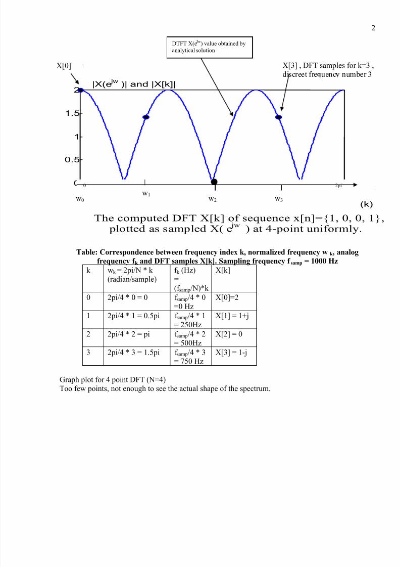
Consider a sequence x[n] = {1, 0, 0, 1}, obtain its 4 points DFT, X [k ] and plot the magnitudespectrum. The discrete time signal x[n] is obtained after sampling using sampling frequency

1000Hz.

Solution

Refer to the slide for detail calculation to get the value for X[k]

N=4 (4 point DFT) . We take 4 points DFT because there are 4 input samples to be processed.k=0, X[0] = 2

k=1, X[1] = 1+j

k=2, X[2] = 0k=3, X[3] = 1-j

The DTFT plot can be obtained by assuming that x[n] consist of only 4 samples and represented by

]3[][][ nnn x

The plot (blue curve) shows the magnitude of the DTFT value for frequency ranging from 0 to thesampling frequency Fs = 1000 Hz . The x-axis shows the frequency w ranging from 0 to 2pi andfrequency index k. You can also convert the frequency representation in the x-axis to anolog

frequency in hertz as shown in the following table.

Take note that the 4 DFT samples is located on the DTFT curve corresponding to the discrete w0

(k=0) , w1 (k=1) , w3 (k=3) , w4 (k=4)

)(1

0

N

n

n j jen xe X

1,,1,0 ][1

0

2

N k en xk X N

n

kn N

j

8/13/2019 DFT notes 2014


2

frequen

Table: Correspondence between frequency index k, normalized frequency w k , analog

frequency f k and DFT samples X[k]. Sampling frequency f samp = 1000 Hz

k wk = 2pi/N * k (radian/sample)

f k (Hz)

=

(f samp/N)*k

X[k]

0 2pi/4 * 0 = 0 f samp/4 * 0=0 Hz

X[0]=2

1 2pi/4 * 1 = 0.5pi f samp/4 * 1

= 250Hz

X[1] = 1+j

2 2pi/4 * 2 = pi f samp/4 * 2= 500Hz

X[2] = 0

3 2pi/4 * 3 = 1.5pi f samp/4 * 3= 750 Hz

X[3] = 1-j

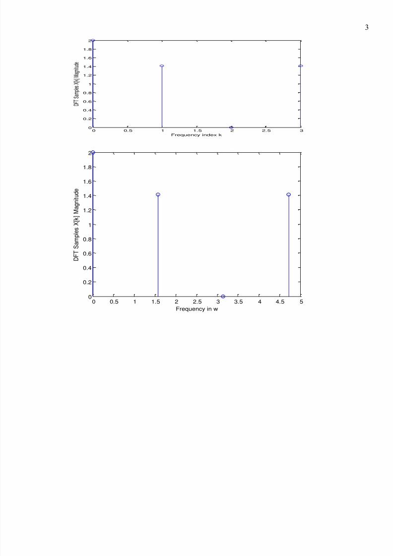
Graph plot for 4 point DFT (N=4)Too few points, not enough to see the actual shape of the spectrum.

0 0.2 0.4 0.6 0.8 10

0.5

1

1.5

2

0 1 2 3 (k)

(w)

|X(e jw

)| and |X[k]|

The computed DFT X[k] of sequence x[n]={1, 0, 0, 1 plotted as sampled X( e

jw) at 4-point uniformly.

0 0.2 0.4 0.6 0.8 10

0.5

1

1.5

2

0 1 2 3 (k)

(w)

|X(e jw

)| and |X[k]|



0 2pi

w0

w1

w2 w3

X[0] X[3] , DFT samples for k=3 ,discreet fre uenc number 3

DTFT X(e w) value obtained by

analytical solution

8/13/2019 DFT notes 2014


3

0 0.5 1 1.5 2 2.5 30

0.2

0.4

0.6

0.8

1

1.2

1.4

1.6

1.8

2

Frequency index k

D F T S

a m p l e s X [ k ] M a g n i t u d e

0 0.5 1 1.5 2 2.5 3 3.5 4 4.5 50

0.2

0.4

0.6

0.8

1

1.2

1.4

1.6

1.8

2

Frequency in w

D F T S a m p l e s X [ k ] M a g n i t u d e

8/13/2019 DFT notes 2014


4

0 100 200 300 400 500 600 700 8000

0.2

0.4

0.6

0.8

1

1.2

1.4

1.6

1.8

2

Frequency in Hz , fsamp =1000Hz

D F T S a m p l e s X [ k ] M a g n i t u

d e

0 100 200 300 400 500 600 700 800 9000

0.2

0.4

0.6

0.8

1

1.2

1.4

1.6

1.8

2



8 Point DFT

8/13/2019 DFT notes 2014


5

0 100 200 300 400 500 600 700 800 900 10000

0.2

0.4

0.6

0.8

1

1.2

1.4

1.6

1.8

2


D F T S a m p l e s X [ k ] M a g n i t u

d e

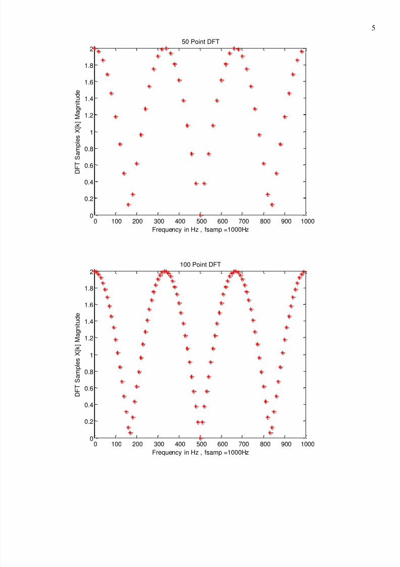
50 Point DFT

0 100 200 300 400 500 600 700 800 900 10000

0.2

0.4

0.6

0.8

1

1.2

1.4

1.6

1.8

2



100 Point DFT

8/13/2019 DFT notes 2014


6

Note that the spectrum of discrete time signal is periodic and repeat every 2pi or every sampling

frequency fsamp. Therefore it is better to plot from the frequency 0-pi or from 0 to fsamp/2

(500Hz)

0 50 100 150 200 250 300 350 400 450 5000

0.2

0.4

0.6

0.8

1

1.2

1.4

1.6

1.8

2


D F T

S a m p l e s X [ k ] M a g n i t u d e

100 Point DFT

In this particular case, we can analytically compute DTFT since we can write the equation for the

signal. The DTFT plot can be obtained by assuming that x[n] consist of only 4 samples {1,0,0,1} andrepresented by ]3[][][ nnn x . After the equation for DTFT signal X(e

jw) is obtained it can be

plotted for various value of w such as 0, pi/8 , pi/4 .

In practical situation that involve spectrum analysis of audio signal or signal captured from the

sensors (such as EEG, ECG), the equation are not known. In this situation, we just need to capture alarge number of samples say N , eg. N=1000. Then do N point DFT. The N/2 DFT samples are

plotted against the N/2 discreet frequencies.

Here are the summarized steps to perform DFT to estimate the spectrum of a captured signal usingthe computer program

Step 1) Capture the signalStep 2) Perform A/D conversion

Step 3) Capture N samples, N is large

Step 4) Do N point DFT to obtain X[k] , k=0,1,2, …N-1

Step 5) Plot X[k] vs the discreet frequencies wk for k=0,1,2 …N/2

8/13/2019 DFT notes 2014


7

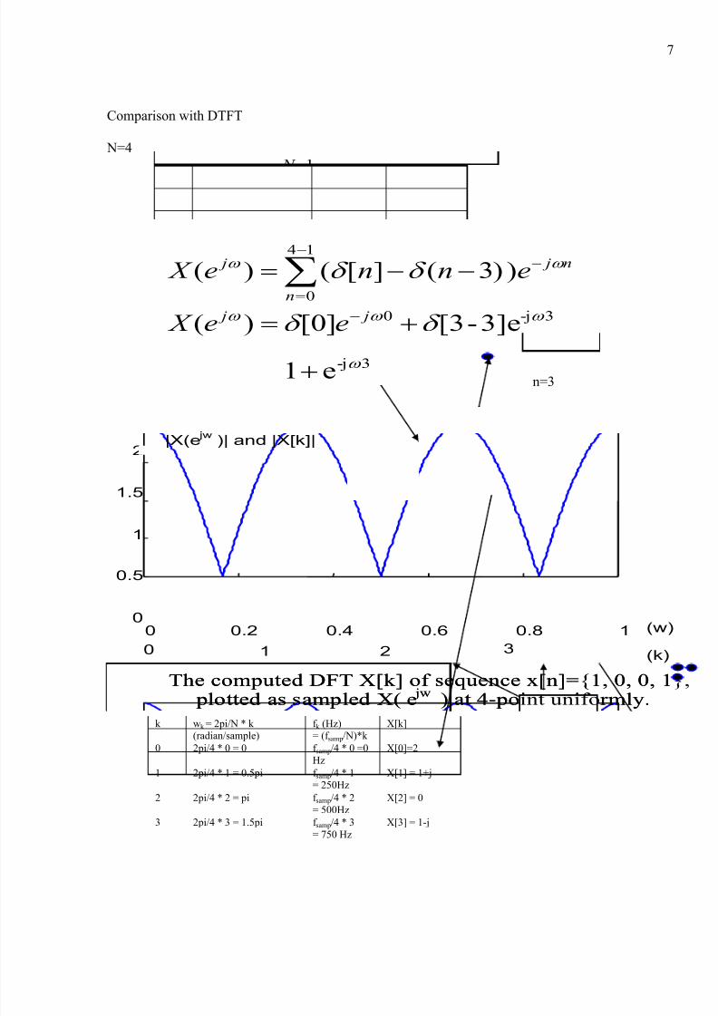
Comparison with DTFT

N=4

k wk = 2pi/N * k (radian/sample)

f k (Hz)= (f samp/N)*k

X[k]

0 2pi/4 * 0 = 0 f samp/4 * 0 =0

Hz

X[0]=2

1 2pi/4 * 1 = 0.5pi f samp/4 * 1= 250Hz

X[1] = 1+j

2 2pi/4 * 2 = pi f samp/4 * 2= 500Hz

X[2] = 0

3 2pi/4 * 3 = 1.5pi f samp/4 * 3

= 750 Hz

X[3] = 1-j

0 0.2 0.4 0.6 0.8 10

0.5

1

1.5

2

0 1 2 3(k)

(w)

|X(e jw

)| and |X[k]|



0 0.2 0.4 0.6 0.8 10

0.5

1

1.5

2

0 1 2 3(k)

(w)

|X(e jw

)| and |X[k]|



))3(][()(14

0

n

n j jenne X

)(1

0

N

n

n j j en xe X

3]e-[3]0[)( 3-j0

j j ee X

e1 3-j

n=3

8/13/2019 DFT notes 2014


8

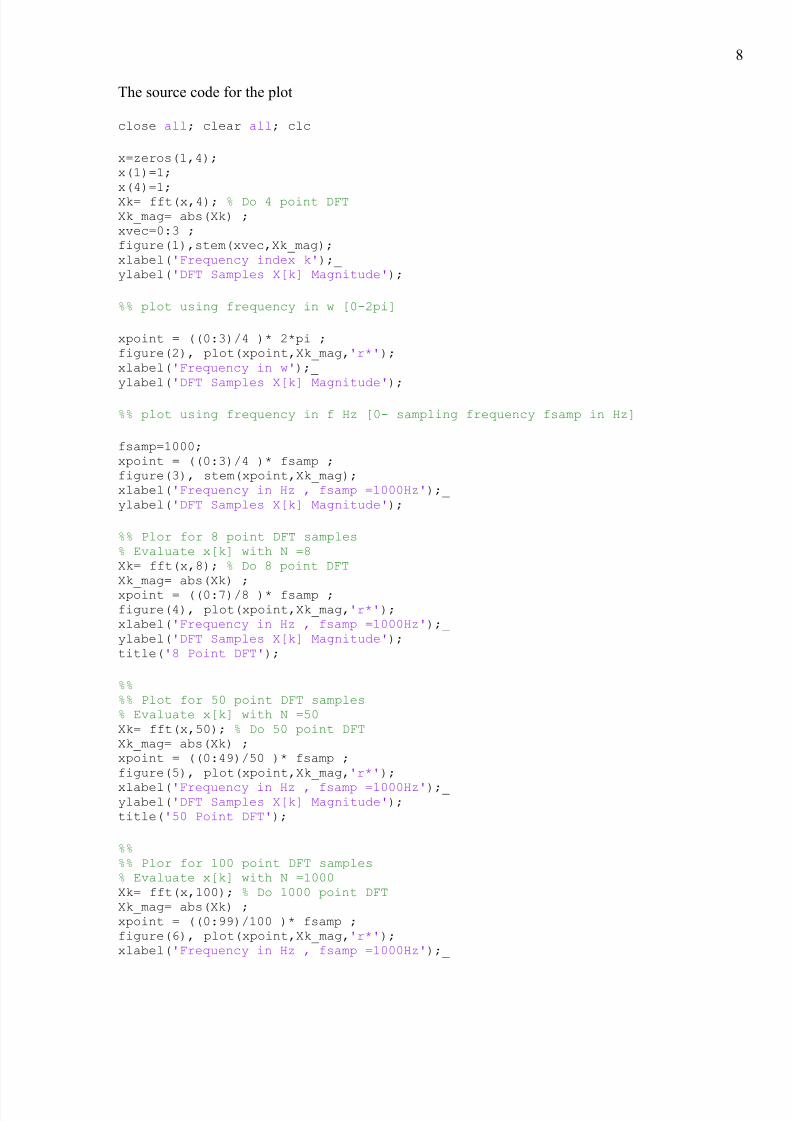
The source code for the plot

close all; clear all; clc

x=zeros(1,4); x(1)=1; x(4)=1; Xk= fft(x,4); % Do 4 point DFT Xk_mag= abs(Xk) ; xvec=0:3 ; figure(1),stem(xvec,Xk_mag); xlabel('Frequency index k');_ ylabel('DFT Samples X[k] Magnitude');

%% plot using frequency in w [0-2pi]

xpoint = ((0:3)/4 )* 2*pi ; figure(2), plot(xpoint,Xk_mag,'r*'); xlabel('Frequency in w');_ ylabel('DFT Samples X[k] Magnitude');

%% plot using frequency in f Hz [0- sampling frequency fsamp in Hz]

fsamp=1000; xpoint = ((0:3)/4 )* fsamp ; figure(3), stem(xpoint,Xk_mag); xlabel('Frequency in Hz , fsamp =1000Hz');_ ylabel('DFT Samples X[k] Magnitude');

%% Plor for 8 point DFT samples % Evaluate x[k] with N =8 Xk= fft(x,8); % Do 8 point DFT Xk_mag= abs(Xk) ; xpoint = ((0:7)/8 )* fsamp ; figure(4), plot(xpoint,Xk_mag,'r*'); xlabel('Frequency in Hz , fsamp =1000Hz');_ ylabel('DFT Samples X[k] Magnitude'); title('8 Point DFT');

%% %% Plot for 50 point DFT samples % Evaluate x[k] with N =50 Xk= fft(x,50); % Do 50 point DFTXk_mag= abs(Xk) ; xpoint = ((0:49)/50 )* fsamp ; figure(5), plot(xpoint,Xk_mag,'r*'); xlabel('Frequency in Hz , fsamp =1000Hz');_ ylabel('DFT Samples X[k] Magnitude'); title('50 Point DFT');

%% %% Plor for 100 point DFT samples % Evaluate x[k] with N =1000 Xk= fft(x,100); % Do 1000 point DFTXk_mag= abs(Xk) ; xpoint = ((0:99)/100 )* fsamp ; figure(6), plot(xpoint,Xk_mag,'r*'); xlabel('Frequency in Hz , fsamp =1000Hz');_

8/13/2019 DFT notes 2014


9ylabel('DFT Samples X[k] Magnitude'); title('100 Point DFT');

%% Plot from 0 till fsamp/2

% for 100 point DFT xfreq = xpoint(1:50); % take half of the frequency points Xk_new = Xk_mag(1:50); % take half of the DFT samples

figure(7), plot(xfreq,Xk_new,'r*'); xlabel('Frequency in Hz , fsamp =1000Hz');_ ylabel('DFT Samples X[k] Magnitude'); title('100 Point DFT');

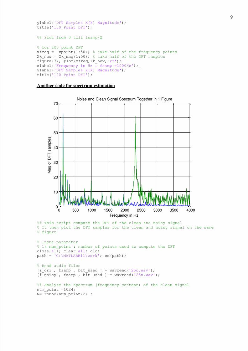
Another code for spectrum estimation

0 500 1000 1500 2000 2500 3000 3500 40000

10

20

30

40

50

60

70

Frequency in Hz

M a g o f D F T s a m p l e s

Noise and Clean Signal Spectrum Together in 1 Figure

%% This script compute the DFT of the clean and noisy signal % It then plot the DFT samples for the clean and noisy signal on the same % figure

% Input parameter % 1) num_point : number of points used to compute the DFTclose all; clear all; clc; path = 'C:\MATLABR11\work'; cd(path);

% Read audio files [i_ori , fsamp , bit_used ] = wavread('25o.wav'); [i_noisy , fsamp , bit_used ] = wavread('25n.wav');

%% Analyze the spectrum (frequency content) of the clean signal num_point =1024;N= round(num_point/2) ;

8/13/2019 DFT notes 2014


10

SClean= fft(i_ori,num_point) ; % create num_point DFT samples from 0 to fsamp %w= (0:(num_point-1))/(num_point/2) * (fsamp/2) ; % frequency in Hz from [0fsamp/2] w= (0:(N-1))/N * (fsamp/2) ; % frequency vector in Hz from [0 fsamp/2] , take Nsamples

plot( w, abs( SClean(1:N) ) ), grid on;

xlabel('Frequency in Hz'); ylabel('Mag of DFT samples for Clean Signal'); title('Clean Signal Spectrum ');

%% Analyze the spectrum (frequency content) of the clean and noisy signal

SNoisy= fft(i_noisy,num_point) ; % create 512 DFT samples from 0 to Fsamp w= (0:(N-1))/N * (fsamp/2) ; % frequency vector in Hz from [0 fsamp/2] , take Nsamples figure, plot( w, abs( [SClean(1:N) SNoisy(1:N)] ) ), grid on; xlabel('Frequency in Hz'); ylabel('Mag of DFT samples'); title('Noise and Clean Signal Spectrum Together in 1 Figure');

Documents

DFT notes 2014