dexin-zhou.pdf

8/10/2019 dexin-zhou.pdf

http://slidepdf.com/reader/full/dexin-zhoupdf 1/50



Dedication

Dedicated to all my family members who raised me and always supported me to pursuemy dreams.



Acknowledgments

I would like to thank my senior project advisors, Greg Landweber and Cliona Golden,for their dedicated discussion and instructions on my project. I also appreciate ProfessorTsu-Yu Tsao for sitting on my board and offering his suggestions from an economicsperspective. Mark Shi, a director of Citigroup’s Counterparty Risk Management, gave methe initial research idea when I mentioned to him that I was interested in the applicationof mathematics in the financial industry in a Chinatown restaurant. Without his help, itwould have been very hard to start this project. Again, I appreciate my family membersfor their unreserved support. Last but not the least, I want to thank all my friends atBard, who treated me like a family member and who gave me courage to move on in thehardest time of my college life.



Abstract

This project is a survey of different aspects of financial risk. My research focuses on thenature of stock price and stock return time series, since it is one of the key factors in thesimulation of returns and losses over a period of time.

The main techniques used in this project are from the field of linear algebra and theFast Fourier Transform (FFT). Time series in nature can be viewed as vectors that live inmulti-dimensions. Therefore, linear algebra naturally arises when dealing with the exist-ing data. The main techniques used are Singular Value Decomposition (SVD) and linearprojection. The former technique examines the orthogonal composition of the data andthe latter examines the relationship of a stock’s projection and the stock return to thetime series itself. The Fast Fourier transform treats stock returns as samples from a signaland identifies the possible patterns out of the stock return time series.

There are two main results. First, the signal processing techniques tell us that there areno obvious regular cycles in stock return time series. Secondly, the stock sector informationreflects in the singular value decomposition. Finally, there are many attempts in thisresearch that are yet to be concluded.



Contents

Dedication 1

Acknowledgments 2

Abstract 3

1 Introduction 6

2 Background Research 9

2.1 Steps in Constructing Value at Risk (VaR) . . . . . . . . . . . . . . . . . . 9

2.2 Variables . . . . . . . . . . . . . . . . . . . . . . . . . . . . . . . . . . . . . 102.3 Other Expressions of VaR . . . . . . . . . . . . . . . . . . . . . . . . . . . . 112.4 Normal Distribution . . . . . . . . . . . . . . . . . . . . . . . . . . . . . . . 11

2.5 Student’s t-distribution . . . . . . . . . . . . . . . . . . . . . . . . . . . . . 122.6 VaR for Parametric Distribution . . . . . . . . . . . . . . . . . . . . . . . . 122.7 Desirable Properties of VaR . . . . . . . . . . . . . . . . . . . . . . . . . . . 13

2.8 Covariance . . . . . . . . . . . . . . . . . . . . . . . . . . . . . . . . . . . . 132.9 Analytic Variance-Covariance, or Delta-Normal Approach . . . . . . . . . . 14

2.10 Delta-Normal VaR for Other Instruments . . . . . . . . . . . . . . . . . . . 152.11 Simulation Method . . . . . . . . . . . . . . . . . . . . . . . . . . . . . . . . 152.12 The Bootstrap . . . . . . . . . . . . . . . . . . . . . . . . . . . . . . . . . . 162.13 C omputing VAR . . . . . . . . . . . . . . . . . . . . . . . . . . . . . . . . . 17

2.14 Simulations with Multiple Variables . . . . . . . . . . . . . . . . . . . . . . 172.15 The Cholesky Factorization . . . . . . . . . . . . . . . . . . . . . . . . . . . 182.16 Number of Independent Factors . . . . . . . . . . . . . . . . . . . . . . . . . 19

2.17 Singular Value Decomposition . . . . . . . . . . . . . . . . . . . . . . . . . . 202.18 Eigenvalues and Singular Values . . . . . . . . . . . . . . . . . . . . . . . . 20



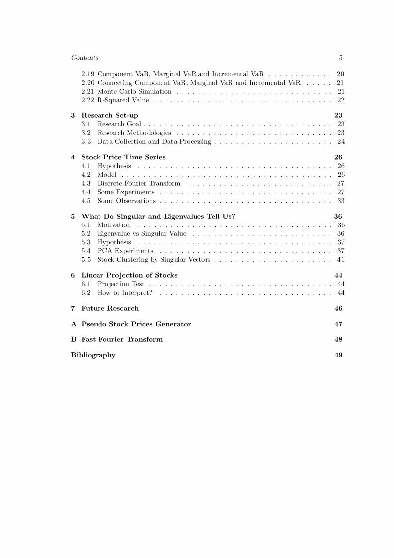
Contents 5

2.19 Component VaR, Marginal VaR and Incremental VaR . . . . . . . . . . . . 202.20 Connecting Component VaR, Marginal VaR and Incremental VaR . . . . . 212.21 Monte Carlo Simulation . . . . . . . . . . . . . . . . . . . . . . . . . . . . . 21

2.22 R -Squared Value . . . . . . . . . . . . . . . . . . . . . . . . . . . . . . . . . 22

3 Research Set-up 23

3.1 Research Goal . . . . . . . . . . . . . . . . . . . . . . . . . . . . . . . . . . . 233.2 Research Methodologies . . . . . . . . . . . . . . . . . . . . . . . . . . . . . 233.3 Data Collection and Data Processing . . . . . . . . . . . . . . . . . . . . . . 24

4 Stock Price Time Series 26

4.1 Hypothesis . . . . . . . . . . . . . . . . . . . . . . . . . . . . . . . . . . . . 264.2 Model . . . . . . . . . . . . . . . . . . . . . . . . . . . . . . . . . . . . . . . 264.3 Discrete Fourier Transform . . . . . . . . . . . . . . . . . . . . . . . . . . . 27

4.4 Some Experiments . . . . . . . . . . . . . . . . . . . . . . . . . . . . . . . . 274.5 Some Observations . . . . . . . . . . . . . . . . . . . . . . . . . . . . . . . . 33

5 What Do Singular and Eigenvalues Tell Us? 36

5.1 Motivation . . . . . . . . . . . . . . . . . . . . . . . . . . . . . . . . . . . . 365.2 Eigenvalue vs Singular Value . . . . . . . . . . . . . . . . . . . . . . . . . . 365.3 Hypothesis . . . . . . . . . . . . . . . . . . . . . . . . . . . . . . . . . . . . 375.4 PCA Experiments . . . . . . . . . . . . . . . . . . . . . . . . . . . . . . . . 375.5 Stock Clustering by Singular Vectors . . . . . . . . . . . . . . . . . . . . . . 41

6 Linear Projection of Stocks 44

6.1 Pro jection Test . . . . . . . . . . . . . . . . . . . . . . . . . . . . . . . . . . 44

6.2 How to Interpret? . . . . . . . . . . . . . . . . . . . . . . . . . . . . . . . . 44

7 Future Research 46

A Pseudo Stock Prices Generator 47

B Fast Fourier Transform 48

Bibliography 49



1

Introduction

Risk is commonly regarded as a concept of the precise probability of specific eventualities.

It is more precisely defined as a state of uncertainty where some of the possibilities in-

volve a loss, catastrophe, or other undesirable outcome. In fact, we face all kinds of risks

throughout our lives. The risks we face in our daily lives include car accidents, sickness,

and investment portfolio depreciation. Therefore, evaluating risks is very important.

To a financial institution, managing risk is always considered one of the top priorities.

Insufficient or badly managed risk can cause significant consequences to the firm. For

instance, AIG’s risk management practices caused the debacle of the insurance giant. The

Credit Default Swap (CDS) contracts that they sold severely damaged the firm’s financial

conditions in the financial crisis. As a result, the AIG stock price fell to below one dollar

from over $60. Another example comes from SocGen of France, where the rogue trader

Jerome Kerviel caused a loss of 4 billion Euros or 7 billion dollars.

People in the financial market face different risks. Usually the risks are categorized

into three categories: market risk, liquidity risk, and credit risk. Value-at-Risk (VAR)

was invented as a measurement of a portfolio’s exposure to all categories’ risks, but it is



1. INTRODUCTION 7

Figure 1.0.1. AIG Stock Prices

most commonly used to measure the market risk. Value at Risk (VaR) is a mathematical

approach for estimating the maximum potential loss of a given portfolio within some period

of time with some likelihood of occurrence. It is sometimes regarded as a barometer for

the trader.

The computation of VaR can be highly dependent on the nature of financial time series.

The historical simulation and Monte-Carlo simulation methods rely heavily on the actual

historical time series and the computer generated time series to predict the future price

movement of certain securities. Therefore, this project focuses on the study of the nature

and charcateristics of financial time series. More specifically, we mainly consider equity

and equity index time series, because the equity market data in the study is more readily

attainable than data from other markets.

Chapter 1 discusses some of the standard computation techniques and theoretical defi-

nitions of Value at Risk. The chapter is followed by an introduction to the research set-up

where the goals, methodologies, data collection and data analysis techniques are intro-

duced. Chapter 4 discusses the analysis that treats stock price and stock return series as

signals and uses Discrete Fourier Transform (DFT) to analyze the data. The following

chapter, What do Singular and eigenvalues tell us? , discusses the results from using sin-



1. INTRODUCTION 8

gular value decomposition and eigen-decomposition to analyze the stock return data. The

linear projection chapter studies the relationship between the linear projection of a stock

onto different set of stocks and the stock time series itself. Finally, we discuss the possible

topics for future research.

Since our question is rather broad, the project is open-ended and the structure of the

project is rather loose. This also reflects the process of the research. We decide to pursue

whatever idea that seems interesting at the time and get partial results. In other words,

this project deals with multiple ideas to try to address the same big question.



2

Background Research

The following discussions and mathematical calculations are standard in academic re-

search. Some of these are direct citations from various sources [1–9].

2.1 Steps in Constructing Value at Risk (VaR)

The steps in constructing the VaR are:

1. Mark to market the current portfolio (the current value of the portfolio on the

market).

2. Measure the variability of risk factors.

3. Set the time horizon.

4. Set the confidence level (the threshold probability that the value.)

5. Report the worst loss by processing all the preceding information.



2. BACKGROUND RESEARCH 10

Example 2.1.1. For instance a $100M portfolio with 15 percent annual volatility (stan-

dard deviation) in 10 days at 99 percent confidence level is

$100M × 15% ×

10 days/252 days × 2.33 = $7M,

where 252 is the approximate number of trading days in a year. ♦

2.2 Variables

The following variables are commonly used in risk management and related probability

and statistics texts. Many of the following variables are similar. Usually, when we are

talking about the current situation, the variables are deterministic (predictable from the

existing information) and variables concerning the future are stochastic (unpredictable

from the existing information.)

• E (.) is the expected value of a variable.

• W is the portfolio/asset value in general. (In the context of a standard textbook, it

usually stands for the value in the future and is stochastic.)

• R is the rate of return. We define R = (W t −W 0)/W 0. (In most contexts, this term

is random, since we are talking about the return in the future.)

• R∗ is the cut off return. It is the maximum loss under the given confidence interval.

(It is a deterministic variable, since the confidence level is given.)

• µ is the mean rate of return. We have µ = E (R). It is deterministic.

• W 0 is the current value of the portfolio or asset. It is a deterministic term, since we

can mark the portfolio to market.

• W ∗ = W 0(1 + R∗) is the cut off value of the portfolio/asset corresponding to R∗. In

general R∗ is negative. Thus we can write it as −|R∗|. It is a deterministic term.






2.5 Student’s t-distribution

The student’s t-distribution is sometimes used to deal with the “fat tail” of stock return

distribution. The probability density function of the student’s t-distribution is

p(x) = Γ(υ+1

2 )√

υπΓ(υ2

)

1 +

x2

υ

−(υ+1

2 )

where

• mean = 0 for υ > 1, otherwise undefined.

• variance = υ/(υ − 2) for υ > 2, otherwise undefined.

2.6 VaR for Parametric Distribution

The VaR computation can be simplified under the assumption that it belongs to a para-

metric family, such as the normal distribution. We translate the general distribution f (w)

to a standard normal distribution Φ().

• R∗ with a standard normal deviate of α > 0 by setting

−α = −|R∗| − µ

σ

is equivalent to setting 1 − c = W ∗

−∞ f (w) dw = −|R∗|−∞ f (r)dr =

−α−∞ Φ()d.

• Standard Normal Cumulative Distribution is N (d) = d

−∞

Φ()d.

• The cut-off return is R∗ = −ασ + µ.

• VAR(mean) = −W 0(R∗ − µ) = W 0ασ√

∆t.

• VAR(zero) = −W 0R∗ = W 0(ασ√

∆t − µ∆t).




2.7 Desirable Properties of VaR

A risk measure can be viewed as a function of the distribution of portfolio value W . Value

at Risk is summarized into a single number ρ(W ) (it can be measured in the dollar value),

with the following properties:

• Monotonicity: If W 1 ≤ W 2, ρ(W 1) ≥ ρ(W 2), or if one portfolio has systemically lower

returns than another for all states of the world, its risk must be greater.

• Translation invariance. ρ(W + k) = ρ(W )

−k, or adding cash k to a portfolio should

reduce its risk by k.

• Homogeneity: ρ(bW ) = bρ(W ), or increasing the size of a portfolio by b should simply

scale its risk by the same factor (this rules out liquidity effects for large portfolios).

• Subadditivity: ρ(W 1 + W 2) ≤ ρ(W 1) + ρ(W 2), or merging portfolios cannot increase

risk.

2.8 Covariance

The covariance between two real-valued random variables X and Y , with expected values

E (x) = µ and E (Y ) = ν is defined as

cov(X, Y ) = E ((X − µ)(Y − ν )).

Covariance can also be expressed as

cov(X, Y ) = ρσxσy,

where ρ is called correlation coefficient and σx and σy are the standard deviation of variable

X and Y .




2.9 Analytic Variance-Covariance, or Delta-Normal Approach

The analytic variance-covariance approach assumes that the distribution of the changes

in portfolio value is normal.

Example 2.9.1. Consider a portfolio with two stocks, with n1 shares of stock 1 valued at

S 1 and n2 shares of stock 2 valued at S 2. The value of the portfolio is W = n1S 1 + n2S 2.

We can select the stock prices S 1 and S 2 as the risk factors. We have:

RW = ∆W

W = n1S 1

W

∆S 1S 1 +

n2S 2W

∆S 2S 2 = ω1R1 + ω2R2,

where

• RW = the rate of return on the portfolio,

• Ri = the rate of return on stock i, i.e, Ri ≡ ∆S i/S i,

• ωi = the percentage of the portfolio invested in stock i.

ωi = 1,

• ∆S is the difference between the security prices at time t and time 0.

Prices are expected to be log-normally distributed, so that the log-returns during the

period (t

−1, t), i.e.,

Rt = ln S tS t−1

= ln

1 − S t − S t−1

S t−1

∼ ∆S t

S t−1,

are normally distributed.

We have RW ∼ N (µW , σW ) with




µW =

2i=1

ωiµi, and

σ2W = ω2

1σ21 + ω2

2σ22 + 2ω1ω2 cov(R1, R2)

= ω21σ2

1 + ω22σ2

2 + 2ω1ω2ρσ1σ2

= (ω1 ω2)

σ2

1 ρσ1σ2

ρσ1σ2 σ22

ω1

ω2

= (ω1 ω2)

σ1 0

0 σ2

ω1

ω2

1 ρρ 1

σ1 0

0 σ2

ω1

ω2

= wΩwT = wσCσwT ,

where w = (ω1 ω2), Ω is the variance-covariance matrix, σ is the diagonal standard

deviation matrix, and C is the correlation matrix. ♦

2.10 Delta-Normal VaR for Other Instruments

We can use a first-order Taylor expansion of the pricing equation to generalize our previous

analysis, giving us

dW =ni=1

∂W

∂f idf i =

ni=1

∆idf i,

where ∆i denotes the “delta” of the position in the instrument. It follows that

σ(dW ) =

ni=1

∆2i σ2(df i) +

ni=1

n j=1,j=i

∆i∆ jcov(df i, df j).

It assumes that the risk factors are normally distributed and the change in asset value

dW is also normally distributed.

2.11 Simulation Method

The first step in the simulation consists of a particular stochastic model for the behavior of

prices. A commonly used model is geometric brownian motion (GBM). The model assumes




that innovations in the asset price are uncorrelated over time and that small movements

in prices can be described by

dS t = µtS tdt + σtS tdz,

where dz is a random variable distributed normally with mean zero and variance dt. It is

assumed that the price of the assets does not depend on random variables. It is Brownian

in the sense that its variance continuously decreases with the time interval, V (dz) = dt.

This rules out processes with sudden jumps.

The variables µt and σt represent the instantaneous drift and volatility at time t. They

evolve over time. The variables µt and σt can be functions of past variables, in which

case it would be easy to simulate time variation in a GARCH (General Autoregressive

Conditional Heteroscedasticity) process.

In practice, the process with infinitesimally small increment dt can be approximated

by discrete moves of size ∆t. Define t as the present time, T as the target time, and

τ = T − t as the (VAR) time horizon. We can first chop τ into n increments, with

∆t = τ/n. (The choice of number of steps should depend on the VAR horizon and the

required accuracy. A smaller number of steps will be faster to implement but may not

provide a good approximation to the stochastic process.)

Integrating ds/s over a finite interval, we have approximately

∆S t = S t−1(µ∆t + σ√

∆t),

where is a standard normal random variable (with mean zero and unit variance). We

have E (∆S/S ) = µ∆t and V (∆S/S ) = σ2∆t.

2.12 The Bootstrap

An alternative to generating random numbers from a hypothetical distribution is to sample

from historical data. Thus we are agnostic about the distribution. For example, suppose




we observe a series of M returns R = ∆S/S , then R = (R1, . . . , RM ), which can

be assumed to be independent identically distributed random variables drawn from an

unknown distribution. The historical simulation methods consist of using this series once

to generate pseudo returns.

2.13 Computing VAR

The steps for simulating VAR are as follows:

1. Choose a stochastic process and parameters.

2. Generate a pseudosequence of variables 1, 2, . . . , n, from which prices are computed

as S t+1, S t+2, . . . , S t+n.

3. Calculate the value of the asset (or portfolio) F t+n = F T under this particular

sequence of prices at the target horizon.

4. Repeat steps 2 and 3 as many times as necessary, i.e. n times.

This process creates a distribution of values F 1T , . . . , F N T . We can sort the observations and

tabulate the expected value E (F T ) and the quantile Q(F T , c). Then

VAR(c, T ) = E (F T ) − Q(F T , c)

2.14 Simulations with Multiple Variables

If the variables are uncorrelated, the randomization can be performed independently for

each variable

∆S j,t = S j,t−1(µ j∆t + σ j j,t√

∆t),

where the values are independent across the time or periods and series j = 1, . . . , N .




Generally, however, variables are correlated. To account for this correlation, we start

with a set of independent variables η , which are then transformed into i variables setting,

1 = η1,

2 = η1 + (1 − ρ2)1/2η2,

where ρ is the correlation coefficient between the variable i. The variable 2 is unity, since

V (2) = ρ2V (η1) + [(1 − ρ2)1/2]2V (η2) = 1. Then the covariance of the i is

cov(1, 2) = cov[η1, ρη1 + (1 − ρ2

)1/2

η2] = ρcov(η1, η2) = ρ.

2.15 The Cholesky Factorization

We suppose that we have a vector of N values of , which we would like to display some

correlation structure V () = E () = R. Since the matrix R is a symmetric real matrix,

it can be decomposed into its Cholesky factors

R = T T ,

where T is a lower triangular matrix with zeros in the upper right corner.

Then start from an N -vector η, which is composed of independent variables all with

unit variances. In other words, V (η) = I , where I is the identity matrix. Next, construct

the variable = T η. Its variance matrix is

V () = E () = E (T ηη T ) = T E (ηη)T = T IT = T T = R.

Thus we have confirmed that the values of have the desired correlations.

For example, in a two-variable case, the matrix can be decomposed into

1 ρρ 1

=

α11 0α12 α22

α11 α12

0 α22

=

α2

11 α11α12

α11α12 α212 + α2

22

.




Because the Cholesky matrix is triangular, the factors can be found by successive substi-

tution by setting

α211 = 1,

α11α12 = ρ,

α212 + α2

22 = 1,

which yields 1 ρρ 1

=

1 0

ρ (1 − ρ2)1/2

η1η2

.

If A has real entries and is symmetric and positive definite, then A can be decomposed

as

A = LLT ,

where L is a lower triangular matrix with strictly positive diagonal entries. If A is a sym-

metric positive-definite matrix with real entries, L can be assumed to have real entries

as well. Cholesky factorization is mainly used for the numerical solution of linear equa-

tions Ax = b. If A is positive definite, then we have A = LLT . Then solve Ly = b for y

and then find LT x = y for x. Cholesky factorization, in our case, helps generate corre-

lated random variables through a variance-covariance matrix (variance-covariance matrix

is positive symmetric).

2.16 Number of Independent Factors

The variable R must be a positive-definite matrix for the decomposition to work. Oth-

erwise, there is no way to transform N independent sources of risks into N correlated

variables of . If the matrix is not positive-definite, the Cholesky factorization will not

work.

We can use the Singular Value Decomposition (principal component analysis) to reduce

the computation without much loss.




2.17 Singular Value Decomposition

Suppose M is an m × n matrix with real entries. Then there exists a factorization of the

form

M = U ΣV T ,

where U is an m×m matrix, Σ is an m×n diagonal matrix with nonnegative numbers on

the diagonal, and V T is an n × n matrix. Such a factorization is called a Singular Value

Decomposition. We have that:

• V contains a set of orthonormal “input” basis vectors for M .

• U contains a set of orthonormal “output” basis for M .

• the matrix Σ contains the singular values.

SVD allows us to truncate the matrix into M = U tΣtV T t , where M is the closest approxi-

mation of rank t to the matrix M .

2.18 Eigenvalues and Singular Values

Eigenvalues and singular values are similar concepts. Suppose the matrix A has column

vectors centered at zero. Then AT A is essentially a covariance matrix, where the entry

ai,j = Ai, A j and the covariance between the columns related to item i and j is σi,j =

ai,jn − 1

. In this case, the eigenvalues of the matrix AT A are just the squares of the singular

values of A multiplied by some normalization constant.

2.19 Component VaR, Marginal VaR and Incremental VaR

Marginal VaR measures the change in return-VaR resulting from a marginal change in

the relative position in instrument i. Hence we have:

M −VAR ≡ ∂r p∂wi

for i ∈ p.






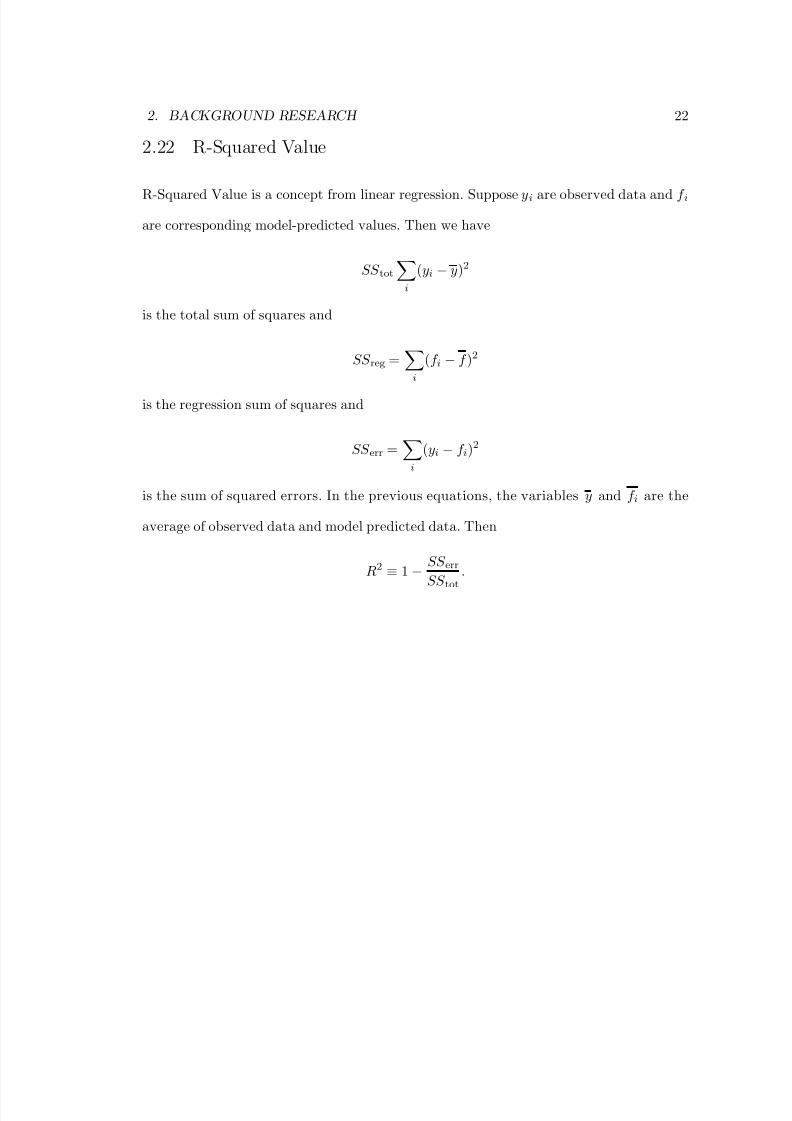
2.22 R-Squared Value

R-Squared Value is a concept from linear regression. Suppose yi are observed data and f i

are corresponding model-predicted values. Then we have

SS toti

(yi − y)2

is the total sum of squares and

SS reg =i

(f i − f )2

is the regression sum of squares and

SS err =i

(yi − f i)2

is the sum of squared errors. In the previous equations, the variables y and f i are the

average of observed data and model predicted data. Then

R2 ≡ 1 − SS errSS

tot

.



3

Research Set-up

3.1 Research Goal

My research goal is to use mathematical tools to identify risks in an equity portfolio. The

research here emphasizes the quantification of Value at Risk. In other words, we try to

quantify the risk in a portfolio with the Value at Risk measurement.

3.2 Research Methodologies

Instead of using purely theoretical mathematical methodologies, I take a different route in

my research. I start by processing data using different techniques and then I try to explain

the theories that justify the findings. The research methodology can be summarized in the

following steps.

1. Data collection and data processing.

2. Data observation.

3. Make a proposition.

4. Test the proposition.



3. RESEARCH SET-UP 24

5. Revise the proposition.

6. Justify the proposition.

3.3 Data Collection and Data Processing

The stock data sample is collected from Google Finance and the index data (Dow Jones

Industrial Average) are collected from Yahoo Finance. Each data point is a close price of

the day. Holidays and weekends, during which there are no trading activities, are excluded

from our data sets.

The data range from January 23rd, 1999 to January 20th, 2009. We may test a chosen

range of time in this range. This time-frame allows us to test the time-series in both the

long term and the short-term.

When choosing stocks for the data sample, I intentionally spread out the sectors of the

stocks so that stocks in different sectors can be tested. The stocks in the sample are listed

as follows:

The components of the sample are as follows.



3. RESEARCH SET-UP 25

No. Stocks Ticker Sector

1 JP Morgan JPM Banking/Financial2 Bank of America BAC Banking/Financial

3 Citi Group C Banking/Financial4 Morgan Stanley MS Banking/Financial5 Wells Fargo WFC Banking/Financial6 MasterCard M Credit Card/Financial7 News Corp NWS Media8 Coca-Cola KO Beverage/Food9 Microsoft MSFT Software/IT

10 Oracle ORCL Database/IT11 WalMart WMT Retail12 ConocoPhillips COP Oil/Commodity13 ExxonMobile XOM Oil/Commodity

14 Chesapeake CHK Oil/Commodity15 XTO Energy XTO Oil/Commodity16 GlaxoSmithKline GSK Drugs17 Pfitzer PFE Drugs18 Rio Tinto PFE Metal Mining/Commodity19 BHP Bilton BHP Metal Mining/Commodity20 Anglo American AAUK Metal Mining/Commodity

Table 3.3.1. Sample Stocks

MATLAB 2007 is the primary tool for the data analysis. The return data matrix is

generated by calculating the log-return using the following formula

rt = log(P t) − log(P t−1)

for each of the stocks.



4

Stock Price Time Series

“It will fluctuate.” - JP Morgan, when asked what the stock market would do.

4.1 Hypothesis

Stock prices change from time to time. Stock price movement is itself a time series. The

stock prices do rise and fall from people’s buying and selling activities. Therefore, there

might be some common frequencies at which stock generate abnormal returns. For in-

stance, in some literatures it is found that the stock prices are generally lower in December

and higher in January. People’s mentality may also contribute to the mean-return of stock

prices in small scales. Therefore, the stock prices or stock returns are not totally random

walks. By using time series analysis, some interesting facts about the stock prices may be

revealed.

4.2 Model

The model is built upon a sunspot model (please refer to Appendix B for the code). The

mathematical tools reveal the relative strength or energy on each of the frequency nodes.



4. STOCK PRICE TIME SERIES 27

That is to say, we will be able to observe the possible abnormal return/stock price change

frequencies.

4.3 Discrete Fourier Transform

The Discrete Fourier Transform (DFT) transforms one function into another. The DFT

is called the frequency domain representation of the original function (which is often a

function defined on the time domain).

The mathematical definition of DFT is as follows [8].

The sequence of N complex numbers x0, . . . , xN −1 is transformed into the sequence of

N complex numbers X 0, . . . , X N −1 by the DFT according to the following formula:

X k =

N −1n=0

xne− 2πi

N kn k = 0, . . . , N − 1,

where e−2πi

N kn is a primitive N’th root of unity.

4.4 Some Experiments

We use MATLAB to examine some of the stock and index time series that we obtained

from various data sources. The JP Morgan time series from January 23rd, 1999 to January

20th, 2009 is:




After performing a DFT, we get




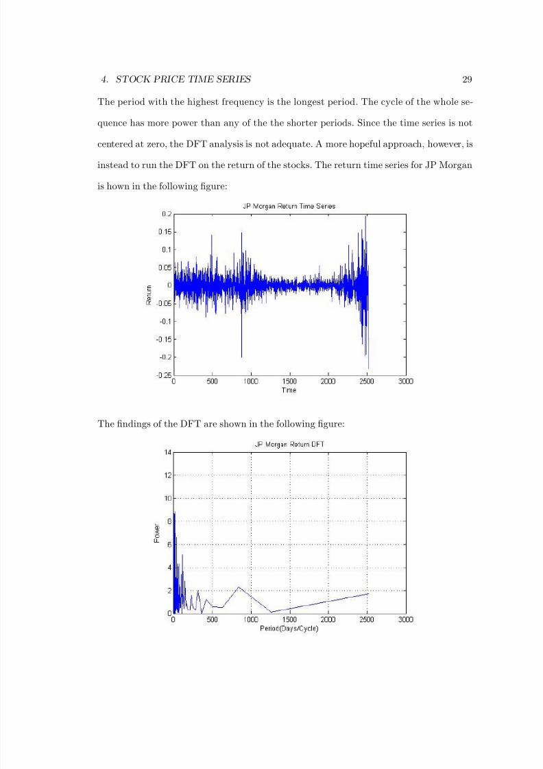
The period with the highest frequency is the longest period. The cycle of the whole se-

quence has more power than any of the the shorter periods. Since the time series is not

centered at zero, the DFT analysis is not adequate. A more hopeful approach, however, is

instead to run the DFT on the return of the stocks. The return time series for JP Morgan

is hown in the following figure:

The findings of the DFT are shown in the following figure:




Besides seeing that the energies are concentrated in the lower period, there is no obvious

conclusion. The experiment is repeated on a few other time series.

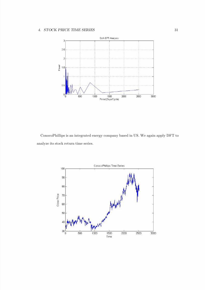
We applied a similar analysis to Dow Jones Industrial Average Index:




ConocoPhillips is an integrated energy company based in US. We again apply DFT to

analyze its stock return time series.




Again, all the time series above display very similar properties under DFT. In the following

section, we will try to explain the behaviors of the stock return time series.




4.5 Some Observations

Despite the unexciting graphs we get from applying the Discrete Fourier Transform, we

can still observe some trends of particular stocks from the graphs. We see 500 days as

a period that covers about two years (there are about 250 trading days in a year). JP

Morgan has a peak at a period close to 3-year cycle. In the shorter term, a scaled image

reveals some facts. With the help of MATLAB’s data cursor, some additional peaks can

be located and tentatively explained.

Days/Cycle Energy Possible Explanations

5.96 11.86 Weekly Fluctuation22.06 8.709 Monthly Fluctuation38.11 6.258 N/A76.21 4.384 Quarterly Fluctuation114.3 4.747 N/A

The Dow Jones Industrial shows a peak on approximately a two-year and one-year cycle.

The 83.77 days/cycle period has relatively strong energy perhaps related to the quarterly

changes. The 228.5 days/cycle period perhaps corresponds to the yearly fluctuation.

ConocoPhillips also has some interesting peaks.

Days/Cycle Energy Possible Explanations

4.03 8.953 Weekly Fluctuation24.9 4.434 Monthly Fluctuation

73.97 2.877 Quarterly Fluctuation86.72 3.33 N/A

251.5 1.829 Semi-Annual Fluctuation838.3 0.8711 N/A

Before getting too optimistic with our findings, let’s examine a random sequence. The

sequence is generated by some simple MatLab codes (please refer to Appendix A). The

sequence is a random walk with fixed variance and zero mean (here 0.01 is specified).




This pseudo return time series is clearly distinct from any stock return time series that

was shown previously. The returns are more bounded and compact in the pseudo return

series and volatility looks uniform throughout the series. The DFT Analysis gives rise to

the following graph:

The pseudo return time series is not that different from the actual stock return! Also, if

we want to, we can assign peaks meanings.




The only observable difference between this and the previous DFT analysis charts is

that the tail of this DFT chart is much higher than the three analyses on the real historical

data, suggesting more energy on the longer periods. Whether this observation is true to

most of the stocks is yet to be concluded.

However, we can see that the cyclical behavior on DFT analysis is mainly a result of

random walk behavior. At least, it is safe to conclude that there is no strong indication of

stocks’ cyclic with fixed frequency.



5

What Do Singular and Eigenvalues Tell Us?

5.1 Motivation

Principal Component Analysis (PCA) can help people indentify the factor that causes

the most impact [12]. PCA plays a very important role in risk management techniques.

The technique can be used to reduce the dimension of a covariance matrix. Besides its

application in Monte Carlo simulation, Principle Component Analysis can also reduce the

computation time of the analytic method. However, the modified matrix using PCA has

a downward bias on the VaR. Whereas people hope to facilitate the computation, under-

estimating risks can cause big problems to risk management. Therefore, it is important

to study the nature of singular and eigenvalues of a matrix, which are central concepts in

PCA.

5.2 Eigenvalue vs Singular Value

Eigenvalues and singular values are the same concept when we treat a covariance matrix,

since the eigen-decomposition already yields a orthogonol basis. In fact, the singular values

are the square roots of the eigenvalues of the covariance times a certain constant. However,



5. WHAT DO SINGULAR AND EIGENVALUES TELL US? 37

when we study the data matrix, singular value decomposition provides a more convenient

way to look at the matrix, since the data matrices are usually not square matrices.

5.3 Hypothesis

The singular value indicates the magnitude of variation in a certain direction. The first

hypothesis is that the more concentrated the portfolio, the greater the size of the corre-

sponding eigenvalues, since more risks will be concentrated on the principal direction.

The second hypothesis is that the relative importance (percentage of the sum of eigenval-

ues) of the dominant eigenvalue will likely decrease as the portfolio diversifies. Conversely,

the relative importance of the least eigenvalue is likely to increase.

The relative magnitude of a singular value is defined as

M relative = σ2

iσ2i

.

5.4 PCA Experiments

Several portfolio configurations have been carried out to test the properties.

The first portfolio stock selection includes five financial stocks. They are JP Morgan,

Bank of America, Citigroup, Morgan Stanley and Wells Fargo. The first diversification

comes from replacing Wells Fargo by News Corp. The second diversified portfolio consists

of JP Morgan, Bank of America, Morgan Stanley, News Corp and Microsoft. The third

diversified portfolio consists of Coca-Cola, Bank of America, Citigroup, Morgan Stanley

and News Corp. The fourth consists of JP Morgan, WalMart, Morgan Stanley, News

Corp and Microsoft. Finally, the last set of stocks has JP Morgan, Bank of America,

ConocoPhillips, Coca-Cola and GlaxoSmithKline. The start date of our testing is January




23rd, 1999. The length of the data that we use is 251 trading days, or approximately one

year.

This experiment shows that our first hypothesis is questionable,

however, the second hypothesis may be valid in some sense. Therefore, additional experi-

ments are carried out.

This time, a different set of portfolios are being tested and, to show the consistency of

the theory, the set of stock selections are tested under different dates.

Stock Pool No. Company Tickers

1 COP XOM CHK XTO BHP2 COP XOM CHK XTO PFE3 COP BAC CHK XTO PFE4 COP BAC JPM XTO PFE




The start dates of the time series are 300 trading days, 600 trading days and 1200 trading

days after Jan 20, 1999 in the three separate trials. The undiversified portfolio includes

4 oil production/refinery firms and one basic material (BHP Bilton), which has a lot of

exposure to oil price. We gradually diversify the portfolio with financial stocks and Pfizer,

a major drug production company.

Experiment 1:

Experiment 2:




Experiment 3:




These experiments in some sense validated our hypothesis, as we observe from the

tables, that the leading singular values decline as we diversify the portfolio compositions.

However, some anomalies also appear. For example, the diversified portfolio has more

relative magnitude on the first singular value than the second and third singular value in

the second experiment. That is to say, after diversifying the portfolio, the variation on the

principal direction does not decrease versus the other directions.

5.5 Stock Clustering by Singular Vectors

Considering the vectoral nature of our time series presentation, I reflected on my early

work on Data Clustering. The question now can be viewed as:“can we use the singular

vectors to cluster stocks?”, which means, stocks with similar movement are set apart from

the rest in the group. For the specific technique on clustering with SVD, please refer to

[11].

Our experiment starts with oil/energy sector, since oil/energy stocks have very strong

comovements due to the signficant influence of oil prices. The five stocks are XOM, XTO,

CHK, COP and BHP.




The test results are as follows, indicating each stock’s corresponding value on the first

singular vector:

Symbol Value

COP -0.3243XOM -0.2607CHK -0.6752XTO -0.5108BHP -0.3318

As we can observe from the table, all singular values are negative. Then some of the stocks

in the set are replaced by stocks from other sectors. For instance, we when we replace COP

by a financial stock, JPM, the result becomes

Symbol Value

COP 0.3290XOM 0.2621CHK 0.7260XTO 0.5431GSK -0.0317

The value corresponding GSK becomes negative while the other values are positive, dis-

tinguishing GSK from the rest of the stocks in the set. Replacing one more stock in the

portfolio, the result is presented as follows:

Symbol Value

COP 0.3623XOM 0.2870CHK 0.8842PFE -0.0531GSK -0.0415

Now we look into a different sector. The financial sector stocks usually have a lot of

comovements. Therefore, we take a set of five financial stocks and apply SVD.

Symbol Value

JPM 0.4464BAC 0.0017

C 0.5294MS 0.6312

WFC 0.3495

As we expected, since all of the stocks are from the same sector, the signs of the corre-

sponding values on the first singular vector are the same. Meanwhile, we notice that the





6

Linear Projection of Stocks

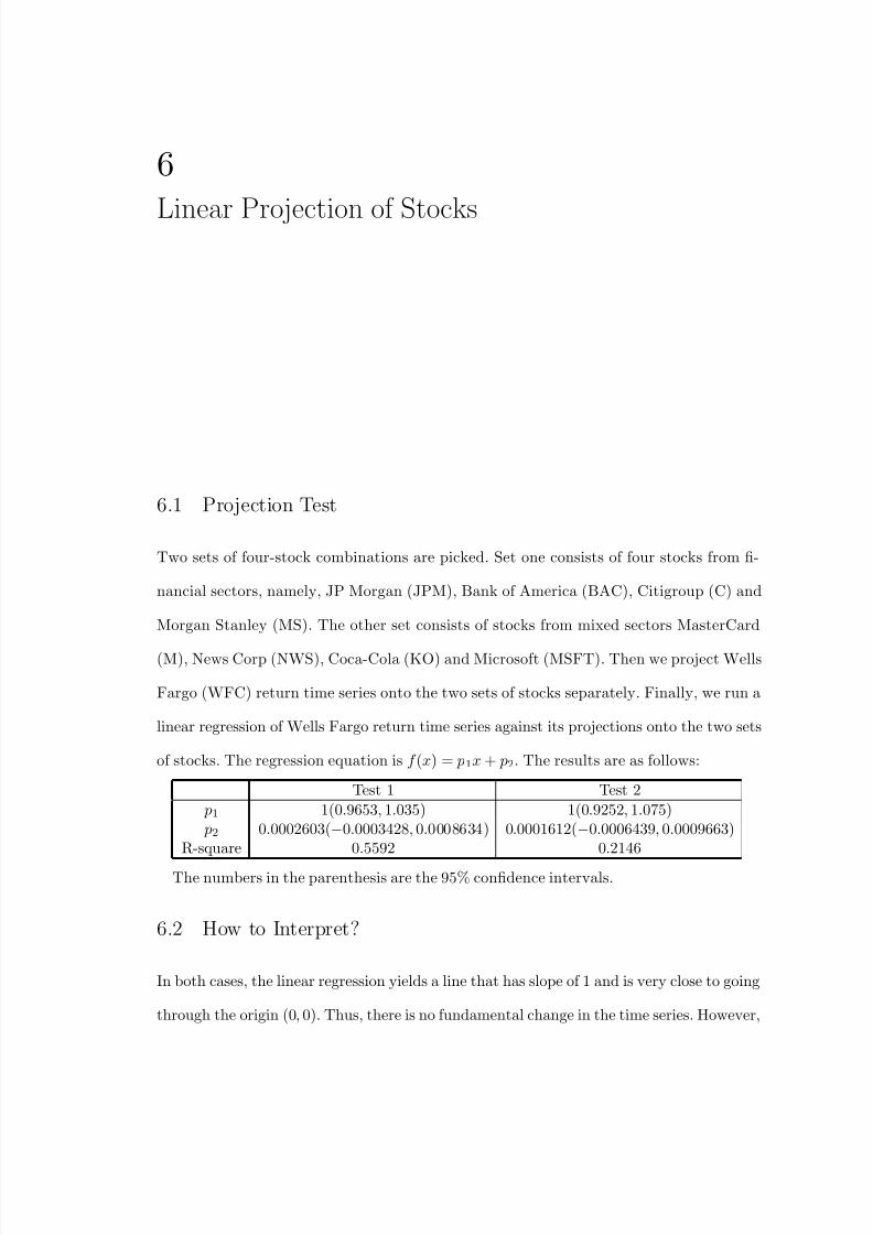
6.1 Projection Test

Two sets of four-stock combinations are picked. Set one consists of four stocks from fi-

nancial sectors, namely, JP Morgan (JPM), Bank of America (BAC), Citigroup (C) and

Morgan Stanley (MS). The other set consists of stocks from mixed sectors MasterCard

(M), News Corp (NWS), Coca-Cola (KO) and Microsoft (MSFT). Then we project Wells

Fargo (WFC) return time series onto the two sets of stocks separately. Finally, we run a

linear regression of Wells Fargo return time series against its projections onto the two sets

of stocks. The regression equation is f (x) = p1x + p2. The results are as follows:

Test 1 Test 2

p1 1(0.9653, 1.035) 1(0.9252, 1.075) p2 0.0002603(−0.0003428, 0.0008634) 0.0001612(−0.0006439, 0.0009663)

R-square 0.5592 0.2146

The numbers in the parenthesis are the 95% confidence intervals.

6.2 How to Interpret?

In both cases, the linear regression yields a line that has slope of 1 and is very close to going

through the origin (0, 0). Thus, there is no fundamental change in the time series. However,



6. LINEAR PROJECTION OF STOCKS 45

the R-square, a variable that explains the total variation explained by the model, dropped

from the first test to the second test. Thus, the projection projected onto the financial

sector is closer to the original series than the one projected onto the mixed sector. Of

course, this result is more or less expected.



7

Future Research

The nature of stock return time series is very intriguing. One direction that particularly

interests me and is, I think, deserving of further research is using signal processing to

analyze the stock return time series. The inconclusiveness of the analysis in this project

could well be a result of the basic nature of the signal processing tool implemented. Some

more sophisticated techniques may tell more interesting stories about the data.

Singular Value Decomposition may provide some previously unidentified relationship

among the stocks in a portfolio. Also, by identifying the greatest direction of variation,

we may be able to hedge the portfolio better by adding a component that counteracts the

risk on that direction.



Appendix A

Pseudo Stock Prices Generator

%This function generates random stock price time series.%mu specifies the average return over the time%sigma specifies the standard deviation of the time series%dt specifies the time interval of each step of simulation%h gives the time horizon (number of days) of the simulation%s0 is the start price (price of day 1)

function sn=gen_s_i(mu,sigma,dt,h,s0)

sn=zeros(1,h); %create a vector that stores the time series.sn(1)=s0; %set the day 1 price to s0epsilon=randn(h-1); %create the drift of each day after day 1 from normal distribufor i=1:h-1

%calculate the prices of each day in the time seriessn(i+1)=sn(i).*(1+mu*dt+sigma.*dt.^(1/2).*epsilon(i));

end



Appendix B

Fast Fourier Transform

%Please refer to MatLab Fourier Analysis Demo

Y = fft(timeseries);N = length(Y);Y(1) = [];power = abs(Y(1:N/2)).^2;nyquist = 1/2;freq = (1:N/2)/(N/2)*nyquist;plot(freq,power), grid on %plot power against frequency

period = 1./freq;plot(period,power), grid on %plot power against period



Bibliography

[1] Philippe Jorion, Value at Risk , 2nd ed., McGraw-Hill Professional, New York, 2000.

[2] Michel Crouchy, Dan Galai, and Robert Mark, Risk Management , 1st ed., McGraw-Hill Professional, New York, 2000.

[3] Darrell Duffie and Jun Pan, An Overview of Value at Risk , Journal of DerivativesSpring (1997), 7-49.

[4] Mark Garman, Ending the Search for Component VaR, http://www.fea.com/

resources/pdf/a_endsearchvar.pdf.

[5] Winfried Hallerbach, Decomposing Portfolio Value-at-Risk , http://www.

smartquant.com/references/VaR/var48.pdf .

[6] Colleen Cassidy and Marianne Gizycki, Measuring Traded Market Risk: Value-At-Risk

and Backtesting Techniques , http://www.rba.gov.au/rdp/rdp9708.pdf.

[7] Mico Loretan, Generating market risk scenarios using principal components analysis:

methodological and practical considerations , http://www.bis.org/publ/ecsc07c.

pdf.

[8] Carl Meyer, Matrix Analysis and Applied Linear Algebra Book , SIAM, Philadelphia,2001.

[9] Steven Lehar, An Intuitive Explanation of Fourier Theory , http://cns-alumni.bu.

edu/~slehar/fourier/fourier.html.

[10] Cleve Moler, Fourier Analysis , http://www.mathworks.com/moler/fourier.pdf.

[11] Ralph Abbey, Jeremy Diepenbrock, Dexin Zhou, Carl Meyer, and Shaina Race, Search

Engines and Data Clustering , http://meyer.math.ncsu.edu/Meyer/REU/REU2007/

Documents

dexin-zhou.pdf