Embed Size (px)
Citation preview
48
CHAPTER 2
Section 2.1 1.
a. S = {1324, 1342, 1423, 1432, 2314, 2341, 2413, 2431, 3124, 3142, 4123, 4132, 3214, 3241, 4213, 4231}.
b. Event A contains the outcomes where 1 is first in the list:
A = {1324, 1342, 1423, 1432}.
c. Event B contains the outcomes where 2 is first or second: B = {2314, 2341, 2413, 2431, 3214, 3241, 4213, 4231}.
d. The event A∪B contains the outcomes in A or B or both:
A∪B = {1324, 1342, 1423, 1432, 2314, 2341, 2413, 2431, 3214, 3241, 4213, 4231}. A∩B = ∅, since 1 and 2 can’t both get into the championship game. A′ = S – A = {2314, 2341, 2413, 2431, 3124, 3142, 4123, 4132, 3214, 3241, 4213, 4231}.
2.
a. A = {RRR, LLL, SSS}. b. B = {RLS, RSL, LRS, LSR, SRL, SLR}. c. C = {RRL, RRS, RLR, RSR, LRR, SRR}. d. D = {RRL, RRS, RLR, RSR, LRR, SRR, LLR, LLS, LRL, LSL, RLL, SLL, SSR, SSL, SRS, SLS, RSS, LSS} e. Event D′ contains outcomes where either all cars go the same direction or they all go different
directions: D′ = {RRR, LLL, SSS, RLS, RSL, LRS, LSR, SRL, SLR}. Because event D totally encloses event C (see the lists above), the compound event C∪D is just event D: C∪D = D = {RRL, RRS, RLR, RSR, LRR, SRR, LLR, LLS, LRL, LSL, RLL, SLL, SSR, SSL, SRS, SLS, RSS, LSS}. Using similar reasoning, we see that the compound event C∩D is just event C: C∩D = C = {RRL, RRS, RLR, RSR, LRR, SRR}.
Chapter 2: Probability
49
3. a. A = {SSF, SFS, FSS}. b. B = {SSS, SSF, SFS, FSS}. c. For event C to occur, the system must have component 1 working (S in the first position), then at least
one of the other two components must work (at least one S in the second and third positions): C = {SSS, SSF, SFS}.
d. C′ = {SFF, FSS, FSF, FFS, FFF}.
A∪C = {SSS, SSF, SFS, FSS}. A∩C = {SSF, SFS}. B∪C = {SSS, SSF, SFS, FSS}. Notice that B contains C, so B∪C = B. B∩C = {SSS SSF, SFS}. Since B contains C, B∩C = C.
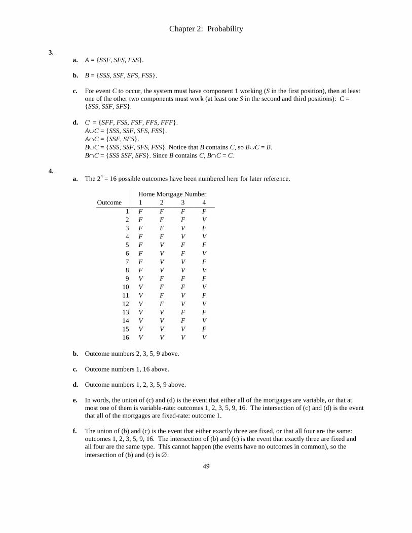
4.
a. The 24 = 16 possible outcomes have been numbered here for later reference.
Home Mortgage Number Outcome 1 2 3 4
1 F F F F 2 F F F V 3 F F V F 4 F F V V 5 F V F F 6 F V F V 7 F V V F 8 F V V V 9 V F F F
10 V F F V 11 V F V F 12 V F V V 13 V V F F 14 V V F V 15 V V V F 16 V V V V
b. Outcome numbers 2, 3, 5, 9 above. c. Outcome numbers 1, 16 above. d. Outcome numbers 1, 2, 3, 5, 9 above. e. In words, the union of (c) and (d) is the event that either all of the mortgages are variable, or that at
most one of them is variable-rate: outcomes 1, 2, 3, 5, 9, 16. The intersection of (c) and (d) is the event that all of the mortgages are fixed-rate: outcome 1.
f. The union of (b) and (c) is the event that either exactly three are fixed, or that all four are the same:
outcomes 1, 2, 3, 5, 9, 16. The intersection of (b) and (c) is the event that exactly three are fixed and all four are the same type. This cannot happen (the events have no outcomes in common), so the intersection of (b) and (c) is ∅.
Chapter 2: Probability
50
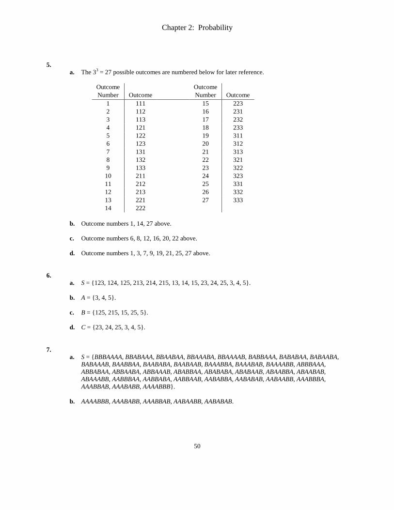
5.
a. The 33 = 27 possible outcomes are numbered below for later reference.
Outcome Outcome Number Outcome Number Outcome
1 111 15 223 2 112 16 231 3 113 17 232 4 121 18 233 5 122 19 311 6 123 20 312 7 131 21 313 8 132 22 321 9 133 23 322 10 211 24 323 11 212 25 331 12 213 26 332 13 221 27 333 14 222
b. Outcome numbers 1, 14, 27 above. c. Outcome numbers 6, 8, 12, 16, 20, 22 above. d. Outcome numbers 1, 3, 7, 9, 19, 21, 25, 27 above.
6.
a. S = {123, 124, 125, 213, 214, 215, 13, 14, 15, 23, 24, 25, 3, 4, 5}.
b. A = {3, 4, 5}. c. B = {125, 215, 15, 25, 5}. d. C = {23, 24, 25, 3, 4, 5}.
7.
a. S = {BBBAAAA, BBABAAA, BBAABAA, BBAAABA, BBAAAAB, BABBAAA, BABABAA, BABAABA, BABAAAB, BAABBAA, BAABABA, BAABAAB, BAAABBA, BAAABAB, BAAAABB, ABBBAAA, ABBABAA, ABBAABA, ABBAAAB, ABABBAA, ABABABA, ABABAAB, ABAABBA, ABAABAB, ABAAABB, AABBBAA, AABBABA, AABBAAB, AABABBA, AABABAB, AABAABB, AAABBBA, AAABBAB, AAABABB, AAAABBB}.
b. AAAABBB, AAABABB, AAABBAB, AABAABB, AABABAB.
Chapter 2: Probability
51
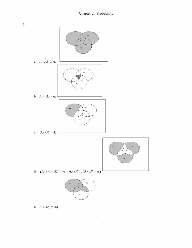
8.
a. A1 ∪ A2 ∪ A3
b. A1 ∩ A2 ∩ A3
c. 1 2 3A AA ′ ′∩ ∩
d. 1 2 3 1 2 3 1 2 3 )(( ) ( )A AA A A A A AA′ ′ ′ ′∩ ∩ ∪ ∩′ ′∩ ∪ ∩ ∩
e. A1 ∪ (A2 ∩ A3)
Chapter 2: Probability
52
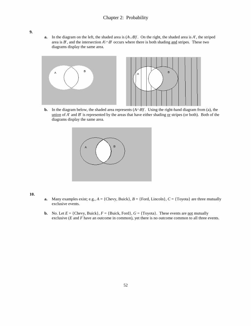
9. a. In the diagram on the left, the shaded area is (A∪B)′. On the right, the shaded area is A′, the striped
area is B′, and the intersection A′∩B′ occurs where there is both shading and stripes. These two diagrams display the same area.
b. In the diagram below, the shaded area represents (A∩B)′. Using the right-hand diagram from (a), the union of A′ and B′ is represented by the areas that have either shading or stripes (or both). Both of the diagrams display the same area.
10.
a. Many examples exist; e.g., A = {Chevy, Buick}, B = {Ford, Lincoln}, C = {Toyota} are three mutually exclusive events.
b. No. Let E = {Chevy, Buick}, F = {Buick, Ford}, G = {Toyota}. These events are not mutually
exclusive (E and F have an outcome in common), yet there is no outcome common to all three events.
Chapter 2: Probability
53
Section 2.2 11.
a. .07. b. .15 + .10 + .05 = .30. c. Let A = the selected individual owns shares in a stock fund. Then P(A) = .18 + .25 = .43. The desired
probability, that a selected customer does not shares in a stock fund, equals P(A′) = 1 – P(A) = 1 – .43 = .57. This could also be calculated by adding the probabilities for all the funds that are not stocks.
12.
a. No, this is not possible. Since event A ∩ B is contained within event B, it must be the case that P(A ∩ B) ≤ P(B). However, .5 > .4.
b. By the addition rule, P(A ∪ B) = .5 + .4 – .3 = .6. c. P(neither A nor B) = P(A′ ∩ B′) = P((A ∪ B)′) = 1 – P(A∪B) = 1 – .6 = .4. d. The event of interest is A∩B′; from a Venn diagram, we see P(A ∩ B′) = P(A) – P(A ∩ B) = .5 – .3 =
.2.
e. From a Venn diagram, we see that the probability of interest is P(exactly one) = P(at least one) – P(both) = P(A ∪ B) – P(A ∩ B) = .6 – .3 = .3.
13.
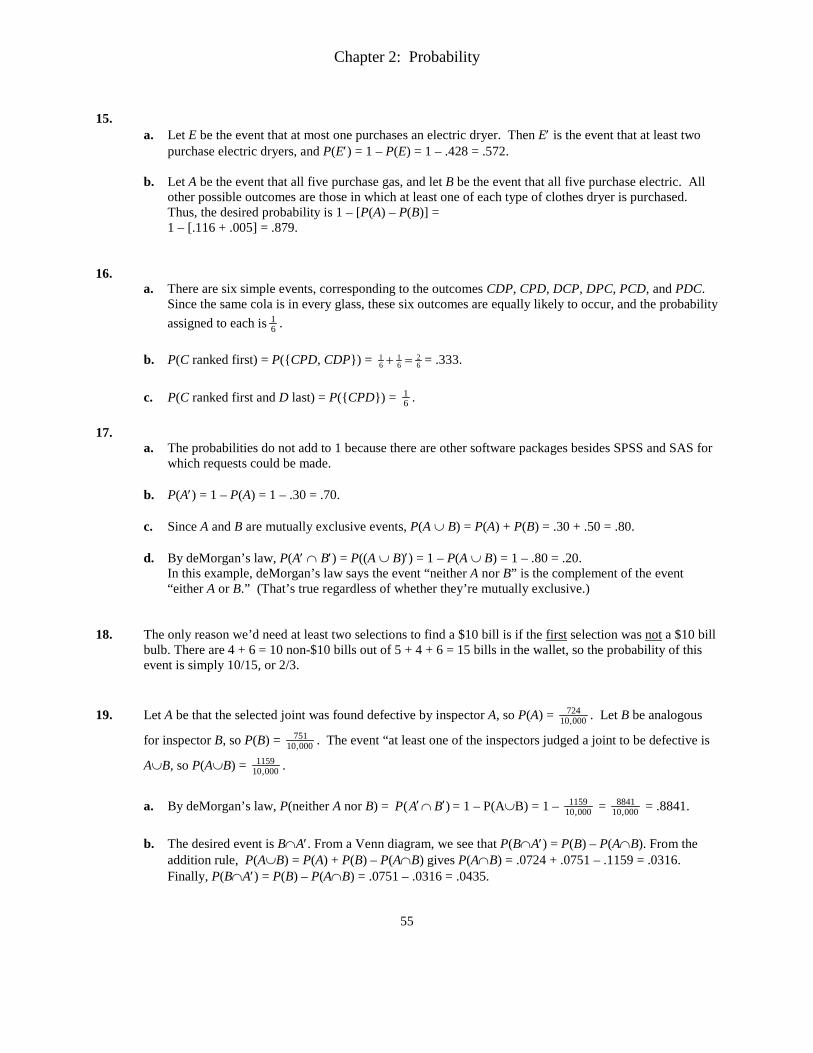
a. 1 2A A∪ = “awarded either #1 or #2 (or both)”: from the addition rule, P(A1 ∪ A2) = P(A1) + P(A2) – P(A1 ∩ A2) = .22 + .25 – .11 = .36.
b. 1 2AA′ ′∩ = “awarded neither #1 or #2”: using the hint and part (a),
1 2 1 2 1 2( ) (( ) ) 1 ( )P A A A P A AP A′ ′∩ ∪ = − ∪′ = = 1 – .36 = .64.
c. 1 2 3A A A∪ ∪ = “awarded at least one of these three projects”: using the addition rule for 3 events,
1 2 3( )AP A A∪ ∪ = 1 2 3 1 2 1 3 2 3 1 2 3) ( ) ( ) ( ) ( ) ( ) )( (P A P A P A A P A A P A A P A A AP A + + − ∩ − ∩ − ∩ + ∩ ∩ = .22 +.25 + .28 – .11 – .05 – .07 + .01 = .53.
d. 1 2 3A AA ′′ ′∩ ∩ = “awarded none of the three projects”: 1 2 3( )AP A A′ ′∩ ∩′ = 1 – P(awarded at least one) = 1 – .53 = .47.
Chapter 2: Probability
54
e. 1 2 3A AA ′′∩ ∩ = “awarded #3 but neither #1 nor #2”: from a Venn diagram,
1 2 3( )A AP A′∩ ∩′ = P(A3) – P(A1 ∩ A3) – P(A2 ∩ A3) + P(A1 ∩ A2 ∩ A3) = .28 – .05 – .07 + .01 = .17. The last term addresses the “double counting” of the two subtractions.
f. 1 2 3( )AA A′∩ ∪′ = “awarded neither of #1 and #2, or awarded #3”: from a Venn diagram,
1 2 3( ))( A AP A′∩ ∪′ = P(none awarded) + P(A3) = .47 (from d) + .28 = 75.
Alternatively, answers to a-f can be obtained from probabilities on the accompanying Venn diagram:
14. Let A = an adult consumes coffee and B = an adult consumes carbonated soda. We’re told that P(A) = .55,
P(B) = .45, and P(A ∪ B) = .70. a. The addition rule says P(A∪B) = P(A) + P(B) – P(A∩B), so .70 = .55 + .45 – P(A∩B) or P(A∩B) = .55
+ .45 – .70 = .30.
b. There are two ways to read this question. We can read “does not (consume at least one),” which means the adult consumes neither beverage. The probability is then P(neither A nor B) = )(P BA′ ′∩ = 1 – P(A ∪ B) = 1 – .70 = .30.
The other reading, and this is presumably the intent, is “there is at least one beverage the adult does not consume, i.e. BA′ ′∪ . The probability is )(P BA′ ′∪ = 1 – P(A ∩ B) = 1 – .30 from a = .70. (It’s just a coincidence this equals P(A ∪ B).) Both of these approaches use deMorgan’s laws, which say that )(P BA′ ′∩ = 1 – P(A∪B) and
)(P BA′ ′∪ = 1 – P(A∩B).
Chapter 2: Probability
55
15.
a. Let E be the event that at most one purchases an electric dryer. Then E′ is the event that at least two purchase electric dryers, and P(E′) = 1 – P(E) = 1 – .428 = .572.
b. Let A be the event that all five purchase gas, and let B be the event that all five purchase electric. All
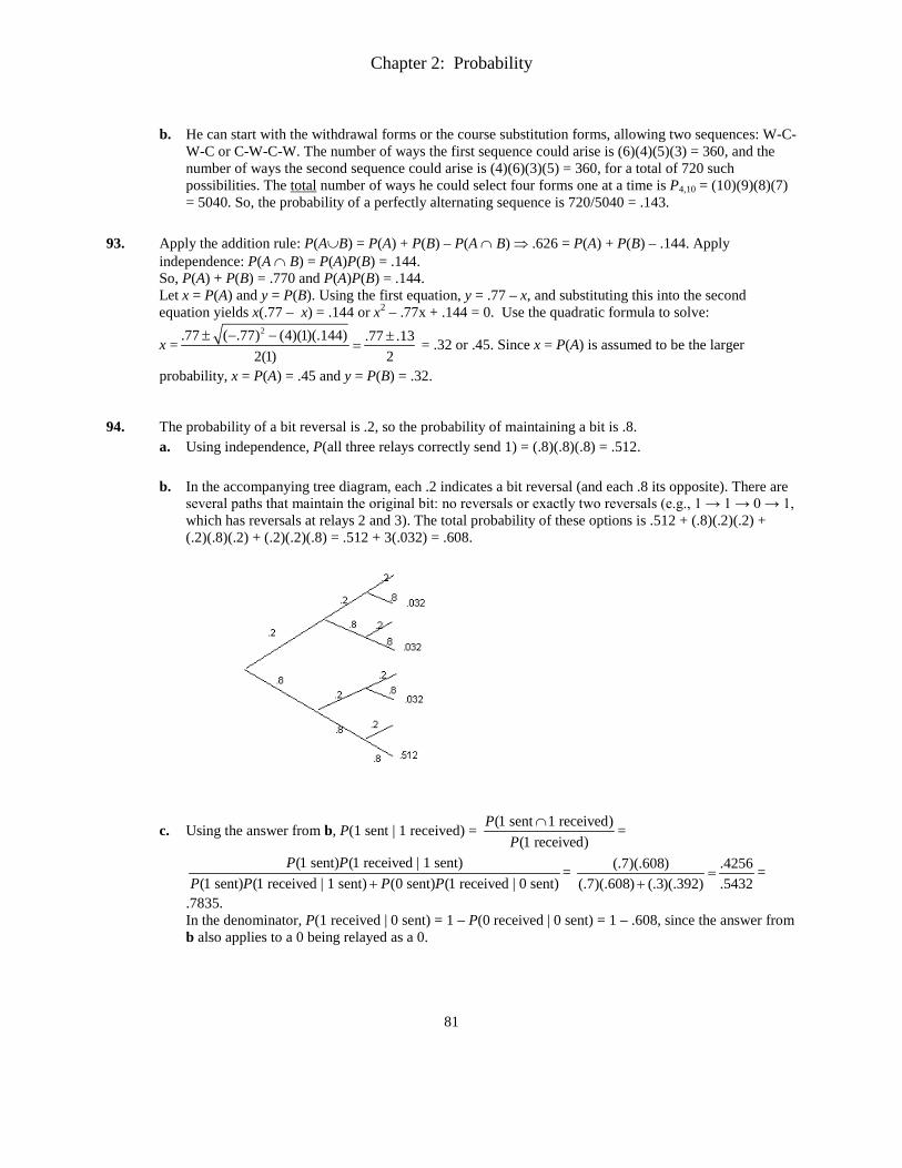
other possible outcomes are those in which at least one of each type of clothes dryer is purchased. Thus, the desired probability is 1 – [P(A) – P(B)] = 1 – [.116 + .005] = .879.
16. a. There are six simple events, corresponding to the outcomes CDP, CPD, DCP, DPC, PCD, and PDC.
Since the same cola is in every glass, these six outcomes are equally likely to occur, and the probability assigned to each is 6
1 . b. P(C ranked first) = P({CPD, CDP}) = 1 1 2
6 6 6+ = = .333. c. P(C ranked first and D last) = P({CPD}) = 6
1 . 17.
a. The probabilities do not add to 1 because there are other software packages besides SPSS and SAS for which requests could be made.
b. P(A′) = 1 – P(A) = 1 – .30 = .70. c. Since A and B are mutually exclusive events, P(A ∪ B) = P(A) + P(B) = .30 + .50 = .80. d. By deMorgan’s law, P(A′ ∩ B′) = P((A ∪ B)′) = 1 – P(A ∪ B) = 1 – .80 = .20.
In this example, deMorgan’s law says the event “neither A nor B” is the complement of the event “either A or B.” (That’s true regardless of whether they’re mutually exclusive.)
18. The only reason we’d need at least two selections to find a $10 bill is if the first selection was not a $10 bill
bulb. There are 4 + 6 = 10 non-$10 bills out of 5 + 4 + 6 = 15 bills in the wallet, so the probability of this event is simply 10/15, or 2/3.
19. Let A be that the selected joint was found defective by inspector A, so P(A) = 000,10
724 . Let B be analogous
for inspector B, so P(B) = 000,10751 . The event “at least one of the inspectors judged a joint to be defective is
A∪B, so P(A∪B) = 000,101159 .
a. By deMorgan’s law, P(neither A nor B) = )(P BA′ ′∩ = 1 – P(A∪B) = 1 – 000,10
1159 = 000,108841 = .8841.
b. The desired event is B∩A′. From a Venn diagram, we see that P(B∩A′) = P(B) – P(A∩B). From the
addition rule, P(A∪B) = P(A) + P(B) – P(A∩B) gives P(A∩B) = .0724 + .0751 – .1159 = .0316. Finally, P(B∩A′) = P(B) – P(A∩B) = .0751 – .0316 = .0435.
Chapter 2: Probability
56
20. a. Let S1, S2 and S3 represent day, swing, and night shifts, respectively. Let C1 and C2 represent unsafe
conditions and unrelated to conditions, respectively. Then the simple events are S1C1, S1C2, S2C1, S2C2, S3C1, S3C2.
b. P(C1)= P({S1C1, S2C1, S3C1})= .10 + .08 + .05 = .23. c. P( 1S ′ ) = 1 – P({S1C1, S1C2}) = 1 – ( .10 + .35) = .55.
21. In what follows, the first letter refers to the auto deductible and the second letter refers to the homeowner’s deductible. a. P(MH) = .10. b. P(low auto deductible) = P({LN, LL, LM, LH}) = .04 + .06 + .05 + .03 = .18. Following a similar
pattern, P(low homeowner’s deductible) = .06 + .10 + .03 = .19. c. P(same deductible for both) = P({LL, MM, HH}) = .06 + .20 + .15 = .41. d. P(deductibles are different) = 1 – P(same deductible for both) = 1 – .41 = .59. e. P(at least one low deductible) = P({LN, LL, LM, LH, ML, HL}) = .04 + .06 + .05 + .03 + .10 + .03 =
.31.
f. P(neither deductible is low) = 1 – P(at least one low deductible) = 1 – .31 = .69. 22. Let A = motorist must stop at first signal and B = motorist must stop at second signal. We’re told that P(A)
= .4, P(B) = .5, and P(A ∪ B) = .6. a. From the addition rule, P(A ∪ B) = P(A) + P(B) – P(A ∩ B), so .6 = .4 + .5 – P(A ∩ B), from which
P(A ∩ B) = .4 + .5 – .6 = .3. b. From a Venn diagram, P(A ∩ B′) = P(A) – P(A ∩ B) = .4 – .3 = .1. c. From a Venn diagram, P(stop at exactly one signal) = P(A ∪ B) – P(A ∩ B) = .6 – .3 = .3. Or, P(stop at
exactly one signal) = P([A ∩ B′]∪ [A′ ∩ B]) = P(A ∩ B′) + P(A′ ∩ B) = [P(A) – P(A ∩ B)] + [P(B) – P(A ∩ B)] = [.4 – .3] + [.5 – .3] = .1 + .2 = .3.
23. Assume that the computers are numbered 1-6 as described and that computers 1 and 2 are the two laptops. There are 15 possible outcomes: (1,2) (1,3) (1,4) (1,5) (1,6) (2,3) (2,4) (2,5) (2,6) (3,4) (3,5) (3,6) (4,5) (4,6) and (5,6).
a. P(both are laptops) = P({(1,2)}) = 15
1 =.067. b. P(both are desktops) = P({(3,4) (3,5) (3,6) (4,5) (4,6) (5,6)}) = 15
6 = .40. c. P(at least one desktop) = 1 – P(no desktops) = 1 – P(both are laptops) = 1 – .067 = .933.
d. P(at least one of each type) = 1 – P(both are the same) = 1 – [P(both are laptops) + P(both are
desktops)] = 1 – [.067 + .40] = .533.
Chapter 2: Probability
57
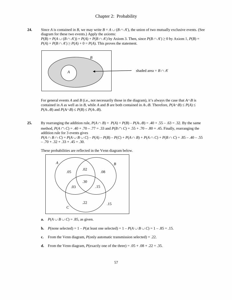
24. Since A is contained in B, we may write B = A ∪ (B ∩ A′), the union of two mutually exclusive events. (See diagram for these two events.) Apply the axioms: P(B) = P(A ∪ (B ∩ A′)) = P(A) + P(B ∩ A′) by Axiom 3. Then, since P(B ∩ A′) ≥ 0 by Axiom 1, P(B) = P(A) + P(B ∩ A′) ≥ P(A) + 0 = P(A). This proves the statement. For general events A and B (i.e., not necessarily those in the diagram), it’s always the case that A∩B is contained in A as well as in B, while A and B are both contained in A∪B. Therefore, P(A∩B) ≤ P(A) ≤ P(A∪B) and P(A∩B) ≤ P(B) ≤ P(A∪B).
25. By rearranging the addition rule, P(A ∩ B) = P(A) + P(B) – P(A∪B) = .40 + .55 – .63 = .32. By the same
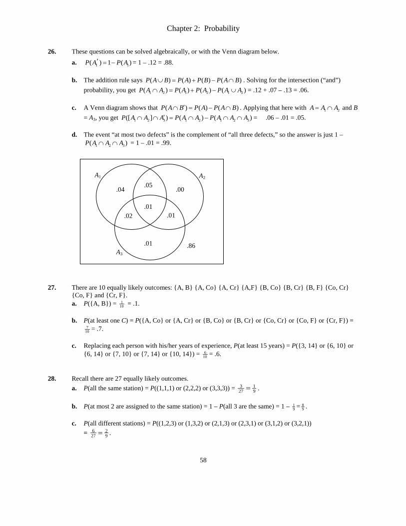
method, P(A ∩ C) = .40 + .70 – .77 = .33 and P(B ∩ C) = .55 + .70 – .80 = .45. Finally, rearranging the addition rule for 3 events gives P(A ∩ B ∩ C) = P(A ∪ B ∪ C) – P(A) – P(B) – P(C) + P(A ∩ B) + P(A ∩ C) + P(B ∩ C) = .85 – .40 – .55 – .70 + .32 + .33 + .45 = .30. These probabilities are reflected in the Venn diagram below.
a. P(A ∪ B ∪ C) = .85, as given. b. P(none selected) = 1 – P(at least one selected) = 1 – P(A ∪ B ∪ C) = 1 – .85 = .15. c. From the Venn diagram, P(only automatic transmission selected) = .22. d. From the Venn diagram, P(exactly one of the three) = .05 + .08 + .22 = .35.
A
B
shaded area = B ∩ A′
.05 .02
.03
.08
.30 .15
.22 .15
A B
C
Chapter 2: Probability
58
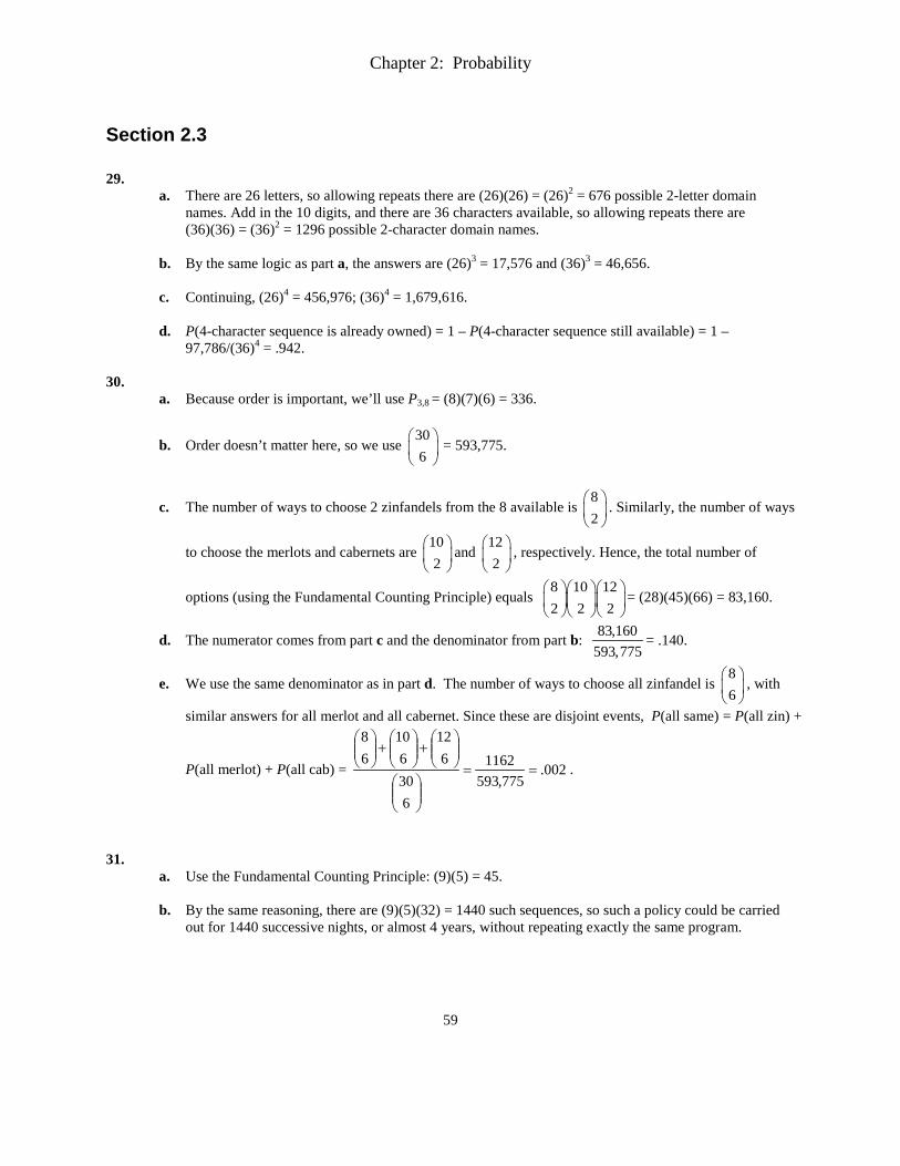
26. These questions can be solved algebraically, or with the Venn diagram below.
a. 1 1( ) 1 ( )P A P A′ = − = 1 – .12 = .88.
b. The addition rule says ) ( )( ( ) ( )P B P A P B A BA P∪ = + − ∩ . Solving for the intersection (“and”) probability, you get 1 2 1 2 1 2) ( ) ( ) ( )( A P A P AP A P A A∩ = + − ∪ = .12 + .07 – .13 = .06.
c. A Venn diagram shows that ) ( ) ( )( B P AP A P A B′∩ = − ∩ . Applying that here with 1 2A AA= ∩ and B
= A3, you get 1 2 3 1 2 1 2 3([ ) ((] ) )P A P AA A A P A A A′∩ − ∩ ∩=∩ ∩ = .06 – .01 = .05.
d. The event “at most two defects” is the complement of “all three defects,” so the answer is just 1 – 1 2 3( )P A A A∩ ∩ = 1 – .01 = .99.
27. There are 10 equally likely outcomes: {A, B} {A, Co} {A, Cr} {A,F} {B, Co} {B, Cr} {B, F} {Co, Cr}
{Co, F} and {Cr, F}. a. P({A, B}) = 1
10 = .1. b. P(at least one C) = P({A, Co} or {A, Cr} or {B, Co} or {B, Cr} or {Co, Cr} or {Co, F} or {Cr, F}) =
710 = .7.
c. Replacing each person with his/her years of experience, P(at least 15 years) = P({3, 14} or {6, 10} or
{6, 14} or {7, 10} or {7, 14} or {10, 14}) = 610 = .6.
28. Recall there are 27 equally likely outcomes. a. P(all the same station) = P((1,1,1) or (2,2,2) or (3,3,3)) = 9
1273 = .
b. P(at most 2 are assigned to the same station) = 1 – P(all 3 are the same) = 1 – 1
9 = 89 .
c. P(all different stations) = P((1,2,3) or (1,3,2) or (2,1,3) or (2,3,1) or (3,1,2) or (3,2,1))
= 92
276 = .
.04
.05
.02
.00
.01 .01
.01 .86
A1 A2
A3
Chapter 2: Probability
59
Section 2.3 29.
a. There are 26 letters, so allowing repeats there are (26)(26) = (26)2 = 676 possible 2-letter domain names. Add in the 10 digits, and there are 36 characters available, so allowing repeats there are (36)(36) = (36)2 = 1296 possible 2-character domain names.
b. By the same logic as part a, the answers are (26)3 = 17,576 and (36)3 = 46,656.
c. Continuing, (26)4 = 456,976; (36)4 = 1,679,616.
d. P(4-character sequence is already owned) = 1 – P(4-character sequence still available) = 1 –
97,786/(36)4 = .942.
30. a. Because order is important, we’ll use P3,8 = (8)(7)(6) = 336.
b. Order doesn’t matter here, so we use 306
= 593,775.
c. The number of ways to choose 2 zinfandels from the 8 available is 82
. Similarly, the number of ways
to choose the merlots and cabernets are 102
and 122
, respectively. Hence, the total number of
options (using the Fundamental Counting Principle) equals 8 10 122 2 2
= (28)(45)(66) = 83,160.
d. The numerator comes from part c and the denominator from part b: 83,160593,775
= .140.
e. We use the same denominator as in part d. The number of ways to choose all zinfandel is 86
, with
similar answers for all merlot and all cabernet. Since these are disjoint events, P(all same) = P(all zin) +
P(all merlot) + P(all cab) = 002.775,593
1162
630
612
610
68
==
+
+
.
31.
a. Use the Fundamental Counting Principle: (9)(5) = 45. b. By the same reasoning, there are (9)(5)(32) = 1440 such sequences, so such a policy could be carried
out for 1440 successive nights, or almost 4 years, without repeating exactly the same program.
Chapter 2: Probability
60
32.
a. Since there are 5 receivers, 4 CD players, 3 speakers, and 4 turntables, the total number of possible selections is (5)(4)(3)(4) = 240.
b. We now only have 1 choice for the receiver and CD player: (1)(1)(3)(4) = 12. c. Eliminating Sony leaves 4, 3, 3, and 3 choices for the four pieces of equipment, respectively:
(4)(3)(3)(3) = 108. d. From a, there are 240 possible configurations. From c, 108 of them involve zero Sony products. So,
the number of configurations with at least one Sony product is 240 – 108 = 132.
e. Assuming all 240 arrangements are equally likely, P(at least one Sony) =132240
= .55.
Next, P(exactly one component Sony) = P(only the receiver is Sony) + P(only the CD player is Sony) + P(only the turntable is Sony). Counting from the available options gives
P(exactly one component Sony) = (1)(3)(3)(3) (4)(1)(3)(3) (4)(3)(3)(1) 99 .413
240 240+ +
= = .
33. a. Since there are 15 players and 9 positions, and order matters in a line-up (catcher, pitcher, shortstop,
etc. are different positions), the number of possibilities is P9,15 = (15)(14)…(7) or 15!/(15–9)! = 1,816,214,440.
b. For each of the starting line-ups in part (a), there are 9! possible batting orders. So, multiply the answer
from (a) by 9! to get (1,816,214,440)(362,880) = 659,067,881,472,000. c. Order still matters: There are P3,5 = 60 ways to choose three left-handers for the outfield and P6,10 =
151,200 ways to choose six right-handers for the other positions. The total number of possibilities is = (60)(151,200) = 9,072,000.
34.
a. Since order doesn’t matter, the number of ways to randomly select 5 keyboards from the 25 available
is 255
= 53,130.
b. Sample in two stages. First, there are 6 keyboards with an electrical defect, so the number of ways to
select exactly 2 of them is 62
. Next, the remaining 5 – 2 = 3 keyboards in the sample must have
mechanical defects; as there are 19 such keyboards, the number of ways to randomly select 3 is 193
.
So, the number of ways to achieve both of these in the sample of 5 is the product of these two counting
numbers: 62
193
= (15)(969) = 14,535.
Chapter 2: Probability
61
c. Following the analogy from b, the number of samples with exactly 4 mechanical defects is 19 64 1
,
and the number with exactly 5 mechanical defects is 195 0
6
. So, the number of samples with at least
4 mechanical defects is 19 64 1
+ 195 0
6
, and the probability of this event is
19 6 19 64 1 5 0
255
+
= 34,88453,130
= .657. (The denominator comes from a.)
35.
a. There are 105
= 252 ways to select 5 workers from the day shift. In other words, of all the ways to
select 5 workers from among the 24 available, 252 such selections result in 5 day-shift workers. Since
the grand total number of possible selections is 245
= 42504, the probability of randomly selecting 5
day-shift workers (and, hence, no swing or graveyard workers) is 252/42504 = .00593.
b. Similar to a, there are 85
= 56 ways to select 5 swing-shift workers and 65
= 6 ways to select 5
graveyard-shift workers. So, there are 252 + 56 + 6 = 314 ways to pick 5 workers from the same shift. The probability of this randomly occurring is 314/42504 = .00739.
c. P(at least two shifts represented) = 1 – P(all from same shift) = 1 – .00739 = .99261. d. There are several ways to approach this question. For example, let A1 = “day shift is unrepresented,”
A2 = “swing shift is unrepresented,” and A3 = “graveyard shift is unrepresented.” Then we want P(A1 ∪ A2 ∪ A3).
N(A1) = N(day shift unrepresented) = N(all from swing/graveyard) =8 6
5
+ = 2002,
since there are 8 + 6 = 14 total employees in the swing and graveyard shifts. Similarly,
N(A2) = 10 6
5 +
= 4368 and N(A3) = 10 8
5 +
= 8568. Next, N(A1 ∩ A2) = N(all from graveyard) = 6
from b. Similarly, N(A1 ∩ A3) = 56 and N(A2 ∩ A3) = 252. Finally, N(A1 ∩ A2 ∩ A3) = 0, since at least one shift must be represented. Now, apply the addition rule for 3 events:
P(A1 ∪ A2 ∪ A3) =2002 4368 8568 6 56 252 0
425014624425044
+ + − − − += = .3441.
36. There are
25
= 10 possible ways to select the positions for B’s votes: BBAAA, BABAA, BAABA, BAAAB,
ABBAA, ABABA, ABAAB, AABBA, AABAB, and AAABB. Only the last two have A ahead of B throughout the vote count. Since the outcomes are equally likely, the desired probability is 2/10 = .20.
Chapter 2: Probability
62
37.
a. By the Fundamental Counting Principle, with n1 = 3, n2 = 4, and n3 = 5, there are (3)(4)(5) = 60 runs. b. With n1 = 1 (just one temperature), n2 = 2, and n3 = 5, there are (1)(2)(5) = 10 such runs.
c. For each of the 5 specific catalysts, there are (3)(4) = 12 pairings of temperature and pressure. Imagine
we separate the 60 possible runs into those 5 sets of 12. The number of ways to select exactly one run
from each of these 5 sets of 12 is 512
1
= 125. Since there are
560
ways to select the 5 runs overall,
the desired probability is 5
5/ 112 60 60
/1 5 5
2 =
= .0456.
38.
a. A sonnet has 14 lines, each of which may come from any of the 10 pages. Order matters, and we’re sampling with replacement, so the number of possibilities is 10 × 10 × … × 10 = 1014.
b. Similarly, the number of sonnets you could create avoiding the first and last pages (so, only using lines from the middle 8 sonnets) is 814. Thus, the probability that a randomly-created sonnet would not use any lines from the first or last page is 814/1014 = .814 = .044.
39. In a-c, the size of the sample space is N = 5 6 4 15
3 3
=
+
+
= 455.
a. There are four 23W bulbs available and 5+6 = 11 non-23W bulbs available. The number of ways to
select exactly two of the former (and, thus, exactly one of the latter) is 4 112 1
= 6(11) = 66. Hence,
the probability is 66/455 = .145.
b. The number of ways to select three 13W bulbs is 53
= 10. Similarly, there are 63
= 20 ways to
select three 18W bulbs and 43
= 4 ways to select three 23W bulbs. Put together, there are 10 + 20 + 4
= 34 ways to select three bulbs of the same wattage, and so the probability is 34/455 = .075.
c. The number of ways to obtain one of each type is 5 6 41 1 1
= (5)(6)(4) = 120, and so the probability
is 120/455 = .264.
d. Rather than consider many different options (choose 1, choose 2, etc.), re-frame the problem this way: at least 6 draws are required to get a 23W bulb iff a random sample of five bulbs fails to produce a 23W bulb. Since there are 11 non-23W bulbs, the chance of getting no 23W bulbs in a sample of size 5
is 11 15
/5 5
= 462/3003 = .154.
Chapter 2: Probability
63
40.
a. If the A’s were distinguishable from one another, and similarly for the B’s, C’s and D’s, then there would be 12! possible chain molecules. Six of these are:
A1A2A3B2C3C1D3C2D1D2B3B1 A1A3A2B2C3C1D3C2D1D2B3B1 A2A1A3B2C3C1D3C2D1D2B3B1 A2A3A1B2C3C1D3C2D1D2B3B1 A3A1A2B2C3C1D3C2D1D2B3B1 A3A2A1B2C3C1D3C2D1D2B3B1
These 6 (=3!) differ only with respect to ordering of the 3 A’s. In general, groups of 6 chain molecules can be created such that within each group only the ordering of the A’s is different. When the A subscripts are suppressed, each group of 6 “collapses” into a single molecule (B’s, C’s and D’s are still distinguishable). At this point there are (12!/3!) different molecules. Now suppressing subscripts on the B’s, C’s, and
D’s in turn gives 4
12 3!(
6 03!)
9,60= chain molecules.
b. Think of the group of 3 A’s as a single entity, and similarly for the B’s, C’s, and D’s. Then there are 4!
= 24 ways to order these triplets, and thus 24 molecules in which the A’s are contiguous, the B’s, C’s,
and D’s also. The desired probability is 24 .00006494369,600
= .
41.
a. (10)(10)(10)(10) = 104 = 10,000. These are the strings 0000 through 9999.
b. Count the number of prohibited sequences. There are (i) 10 with all digits identical (0000, 1111, …, 9999); (ii) 14 with sequential digits (0123, 1234, 2345, 3456, 4567, 5678, 6789, and 7890, plus these same seven descending); (iii) 100 beginning with 19 (1900 through 1999). That’s a total of 10 + 14 + 100 = 124 impermissible sequences, so there are a total of 10,000 – 124 = 9876 permissible sequences.
The chance of randomly selecting one is just 987610,000
= .9876.
c. All PINs of the form 8xx1 are legitimate, so there are (10)(10) = 100 such PINs. With someone
randomly selecting 3 such PINs, the chance of guessing the correct sequence is 3/100 = .03.
d. Of all the PINs of the form 1xx1, eleven is prohibited: 1111, and the ten of the form 19x1. That leaves 89 possibilities, so the chances of correctly guessing the PIN in 3 tries is 3/89 = .0337.
42.
a. If Player X sits out, the number of possible teams is 3 4 41 2 2
= 108. If Player X plays guard, we
need one more guard, and the number of possible teams is3 4 41 21
= 72. Finally, if Player X plays
forward, we need one more forward, and the number of possible teams is 3 4 41 2 1
= 72. So, the
total possible number of teams from this group of 12 players is 108 + 72 + 72 = 252.
b. Using the idea in a, consider all possible scenarios. If Players X and Y both sit out, the number of
possible teams is 3 5 51 2 2
= 300. If Player X plays while Player Y sits out, the number of possible
Chapter 2: Probability
64
teams is 3 5 51 1 2
+3 5 51 2 1
= 150 + 150 = 300. Similarly, there are 300 teams with Player X
benched and Player Y in. Finally, there are three cases when X and Y both play: they’re both guards, they’re both forwards, or they split duties. The number of ways to select the rest of the team under
these scenarios is 3 5 51 0 2
+ 3 5 51 2 0
+ 3 5 51 1 1
= 30 + 30 + 75 = 135.
Since there are 155
= 3003 ways to randomly select 5 players from a 15-person roster, the probability
of randomly selecting a legitimate team is300 300 135
3003+ +
=735
3003= .245.
43. There are 525
= 2,598,960 five-card hands. The number of 10-high straights is (4)(4)(4)(4)(4) = 45 = 1024
(any of four 6s, any of four 7s, etc.). So, P(10 high straight) = 1024 .0003942,598,960
= . Next, there ten “types
of straight: A2345, 23456, …, 910JQK, 10JQKA. So, P(straight) = 102410 .003942,598,960
× = . Finally, there
are only 40 straight flushes: each of the ten sequences above in each of the 4 suits makes (10)(4) = 40. So,
P(straight flush) = 40 .000015392,598,960
= .
44.
−
=−
=−
=
kn
nkkn
nknk
nkn
!)!(!
)!(!!
The number of subsets of size k equals the number of subsets of size n – k, because to each subset of size k there corresponds exactly one subset of size n – k: the n – k objects not in the subset of size k. The combinations formula counts the number of ways to split n objects into two subsets: one of size k, and one of size n – k.
Chapter 2: Probability
65
Section 2.4 45.
a. P(A) = .106 + .141 + .200 = .447, P(C) =.215 + .200 + .065 + .020 = .500, and P(A ∩ C) = .200.
b. P(A|C) = 400.500.200.
)()(
==∩CP
CAP . If we know that the individual came from ethnic group 3, the
probability that he has Type A blood is .40. P(C|A) = ( )( )
P A CP A∩
=
.200
.447= .447. If a person has Type A
blood, the probability that he is from ethnic group 3 is .447. c. Define D = “ethnic group 1 selected.” We are asked for P(D|B′). From the table, P(D∩B′) = .082 +
.106 + .004 = .192 and P(B′) = 1 – P(B) = 1 – [.008 + .018 + .065] = .909. So, the desired probability is
P(D|B′) = 211.909.192.
)()(
==′′∩
BPBDP .
46. Let A be that the individual is more than 6 feet tall. Let B be that the individual is a professional basketball
player. Then P(A|B) = the probability of the individual being more than 6 feet tall, knowing that the individual is a professional basketball player, while P(B|A) = the probability of the individual being a professional basketball player, knowing that the individual is more than 6 feet tall. P(A|B) will be larger. Most professional basketball players are tall, so the probability of an individual in that reduced sample space being more than 6 feet tall is very large. On the other hand, the number of individuals that are pro basketball players is small in relation to the number of males more than 6 feet tall.
47.
a. Apply the addition rule for three events: P(A ∪ B ∪ C) = .6 + .4 + .2 – .3 – .15 – .1 + .08 = .73. b. P(A ∩ B ∩ C′) = P(A ∩ B) – P(A ∩ B ∩ C) = .3 – .08 = .22.
c. P(B|A) = ( ) .3 .50( ) .6
P A BP A∩
= = and P(A|B) = ( ) .3 .75( ) .4
P A BP B∩
= = . Half of students with Visa cards also
have a MasterCard, while three-quarters of students with a MasterCard also have a Visa card.
d. P(A ∩ B | C) = ([ ] ) ( ) .08( ) ( ) .2
P A B P A BP C P C
C C∩ ∩= =
∩ ∩ = .40.
e. P(A ∪ B | C) = ([ ] ) ([ [ )( ) ( )
] ]P A B P A BP C P C
C C C∪ ∩ ∩ ∪ ∩= . Use a distributive law:
= ( ) ([)
) ( ])(
] [P C P CA B P AP C
C B C∩ + ∩ ∩ ∩ ∩− = ( ) (( )
) ( )CP A B PP C CAP
BC
−∩ + ∩ ∩ ∩ =
.15 .1 .08.2
+ − = .85.
Chapter 2: Probability
66
48.
a. 2 12 1
1
( ) .06( | )( ) .12
P A AA
AP
P A ∩= = = .50. The numerator comes from Exercise 26.
b. 1 2 3 1 1 2 31 2 3 1
1 1
) ) .01| ([ ])( ) ( ) . 2
(1
(P A PA A A A AA A AP
AP AA P A
∩ ∩ ∩ ∩ ∩∩ ∩ = = = = .0833. The numerator
simplifies because 1 2 3A A A∩ ∩ is a subset of A1, so their intersection is just the smaller event. c. For this example, you definitely need a Venn diagram. The seven pieces of the partition inside the
three circles have probabilities .04, .05, .00, .02, .01, .01, and .01. Those add to .14 (so the chance of no defects is .86). Let E = “exactly one defect.” From the Venn diagram, P(E) = .04 + .00 + .01 = .05. From the addition above, P(at least one defect) = 1 2 3( )AP A A∪ ∪ = .14. Finally, the answer to the question is
1 2 31 2 3
1 2 3 1 2 3
[ ) ) .05)) ) .14
( ] (( |( (
P E A P EP E AP A P A
A AA AA A A A
∩ ∪ ∪∪ ∪ = = =
∪ ∪ ∪ ∪= .3571. The numerator
simplifies because E is a subset of 1 2 3A A A∪ ∪ .
d. 3 1 23 1 2
1 2
[ ) .05)) .0
(6
( ]|(
AP A AP A AP A
AA
∩ ∩=
∩′
′ ∩ = = .8333. The numerator is Exercise 26(c), while the
denominator is Exercise 26(b). 49.
a. P(small cup) = .14 + .20 = .34. P(decaf) = .20 + .10 + .10 = .40.
b. P(decaf | small) = decaf )(small .20(small) .34
PP
=∩ = .588. 58.8% of all people who purchase a small cup of
coffee choose decaf.
c. P(small | decaf) = decaf )(small .20(decaf ) .40
PP
=∩ = .50. 50% of all people who purchase decaf coffee choose
the small size.
50. a. P(M ∩ LS ∩ PR) = .05, directly from the table of probabilities. b. P(M ∩ Pr) = P(M ∩ LS ∩ PR) + P(M ∩ SS ∩ PR) = .05 + .07 = .12. c. P(SS) = sum of 9 probabilities in the SS table = .56. P(LS) = 1 – .56 = .44. d. From the two tables, P(M) = .08 + .07 + .12 + .10 + .05 + .07 = .49. P(Pr) = .02 + .07 + .07 + .02 + .05
+ .02 = .25.
e. P(M|SS ∩ Pl) = ( ) .08 .533( ) .04 .08 .03
PP∩
= =+
∩∩ +
M SS PlSS Pl
.
f. P(SS|M ∩ Pl) = ( ) .08 .444( ) .08 .10
PP
∩ ∩= =
∩ +SS M Pl
M Pl. P(LS|M ∩ Pl) = 1 – P(SS|M ∩ Pl) = 1 – .444 =
.556.
Chapter 2: Probability
67
51.
a. Let A = child has a food allergy, and R = child has a history of severe reaction. We are told that P(A) = .08 and P(R | A) = .39. By the multiplication rule, P(A ∩ R) = P(A) × P(R | A) = (.08)(.39) = .0312.
b. Let M = the child is allergic to multiple foods. We are told that P(M | A) = .30, and the goal is to find P(M). But notice that M is actually a subset of A: you can’t have multiple food allergies without having at least one such allergy! So, apply the multiplication rule again: P(M) = P(M ∩ A) = P(A) × P(M | A) = (.08)(.30) = .024.
52. We know that P(A1 ∪ A2) = .07 and P(A1 ∩ A2) = .01, and that P(A1) = P(A2) because the pumps are
identical. There are two solution methods. The first doesn’t require explicit reference to q or r: Let A1 be the event that #1 fails and A2 be the event that #2 fails. Apply the addition rule: P(A1 ∪ A2) = P(A1) + P(A2) – P(A1 ∩ A2) ⇒ .07 = 2P(A1) – .01 ⇒ P(A1) = .04. Otherwise, we assume that P(A1) = P(A2) = q and that P(A1 | A2) = P(A2 | A1) = r (the goal is to find q). Proceed as follows: .01 = P(A1 ∩ A2) = P(A1) P(A2 | A1) = qr and .07 = P(A1 ∪ A2) =
1 2 1 2 1 2) (( )( )P A P AA A P A A′∩ + ∩ + ∩′ = .01 + q(1 – r) + q(1 – r) ⇒ q(1 – r) = .03. These two equations give 2q – .01 = .07, from which q = .04 (and r = .25).
53. P(B|A) = )()(
)()(
APBP
APBAP
=∩ (since B is contained in A, A ∩ B = B)
= 0833.60.05.
=
54.
a. P(A2 | A1) = 50.22.11.
)()(
1
21 ==∩AP
AAP. If the firm is awarded project 1, there is a 50% chance they will
also be awarded project 2.
b. P(A2 ∩ A3 | A1) = 0455.22.01.
)()(
1
321 ==∩∩
APAAAP
. If the firm is awarded project 1, there is a 4.55%
chance they will also be awarded projects 2 and 3.
c. )(
)]()[()(
)]([)|(
1
3121
1
321132 AP
AAAAPAP
AAAPAAAP
∩∪∩=
∪∩=∪
682.22.15.
)()()()(
1
3213121 ==∩∩−∩+∩
=AP
AAAPAAPAAP. If the firm is awarded project 1, there is
a 68.2% chance they will also be awarded at least one of the other two projects.
d. 0189.53.01.
)()(
)|(321
321321321 ==
∪∪∩∩
=∪∪∩∩AAAPAAAP
AAAAAAP . If the firm is awarded at least one
of the projects, there is a 1.89% chance they will be awarded all three projects.
Chapter 2: Probability
68
55. Let A = {carries Lyme disease} and B = {carries HGE}. We are told P(A) = .16, P(B) = .10, and P(A ∩ B |
A ∪ B) = .10. From this last statement and the fact that A∩B is contained in A∪B,
.10 = ( )( )
P A BP A B
∩∪
⇒ P(A ∩ B) = .10P(A ∪ B) = .10[P(A) + P(B) – P(A ∩ B)] = .10[.10 + .16 – P(A ∩ B)] ⇒
1.1P(A ∩ B) = .026 ⇒ P(A ∩ B) = .02364.
Finally, the desired probability is P(A | B) = ( ) .02364( ) .10
P A BP B∩
= = .2364.
56. 1)()(
)()()(
)()(
)()()|()|( ==
∩′+∩=
∩′+
∩=′+
BPBP
BPBAPBAP
BPBAP
BPBAPBAPBAP
57. P(B | A) > P(B) iff P(B | A) + P(B′ | A) > P(B) + P(B′|A) iff 1 > P(B) + P(B′|A) by Exercise 56 (with the
letters switched). This holds iff 1 – P(B) > P(B′ | A) iff P(B′) > P(B′ | A), QED.
58. )(
)]()[()(
))[()|(CP
CBCAPCP
CBAPCBAP ∩∪∩=
∩∪=∪
)()()()(
CPCBAPCBPCAP ∩∩−∩+∩
= = P(A |
C) + P(B | C) – P(A ∩ B | C) 59. The required probabilities appear in the tree diagram below.
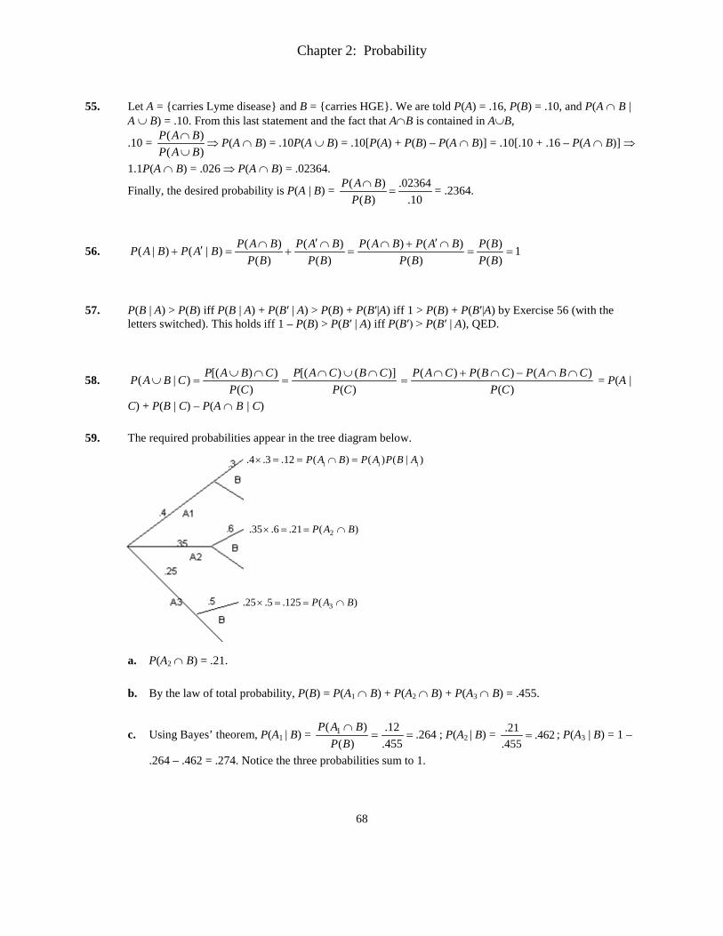
a. P(A2 ∩ B) = .21. b. By the law of total probability, P(B) = P(A1 ∩ B) + P(A2 ∩ B) + P(A3 ∩ B) = .455.
c. Using Bayes’ theorem, P(A1 | B) = 264.455.12.
)()( 1 ==
∩BP
BAP; P(A2 | B) = 462.
455.21.
= ; P(A3 | B) = 1 –
.264 – .462 = .274. Notice the three probabilities sum to 1.
1 11.4 .3 .12 ( ) ( ) ( | )P A B P A P B A× = = ∩ =
)(21.6.35. 2 BAP ∩==×
)(125.5.25. 3 BAP ∩==×
Chapter 2: Probability
69
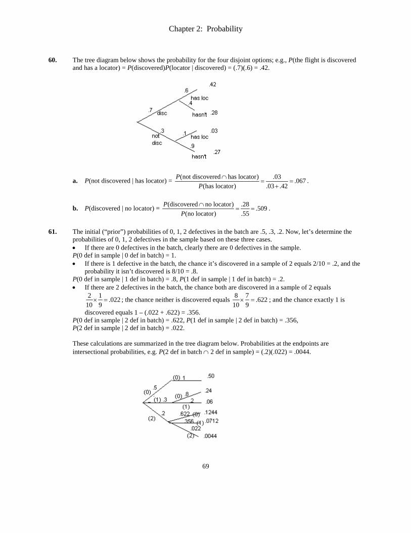
60. The tree diagram below shows the probability for the four disjoint options; e.g., P(the flight is discovered
and has a locator) = P(discovered)P(locator | discovered) = (.7)(.6) = .42.
a. P(not discovered | has locator) = (not discovered has locator) .03 .067(has locator) .03 .42
PP
∩= =
+.
b. P(discovered | no locator) = (discovered no locator) .28 .509(no locator) .55
PP
∩= = .
61. The initial (“prior”) probabilities of 0, 1, 2 defectives in the batch are .5, .3, .2. Now, let’s determine the
probabilities of 0, 1, 2 defectives in the sample based on these three cases. • If there are 0 defectives in the batch, clearly there are 0 defectives in the sample. P(0 def in sample | 0 def in batch) = 1. • If there is 1 defective in the batch, the chance it’s discovered in a sample of 2 equals 2/10 = .2, and the
probability it isn’t discovered is 8/10 = .8. P(0 def in sample | 1 def in batch) = .8, P(1 def in sample | 1 def in batch) = .2. • If there are 2 defectives in the batch, the chance both are discovered in a sample of 2 equals
2 1 .02210 9
× = ; the chance neither is discovered equals 8 7 .62210 9
× = ; and the chance exactly 1 is
discovered equals 1 – (.022 + .622) = .356. P(0 def in sample | 2 def in batch) = .622, P(1 def in sample | 2 def in batch) = .356, P(2 def in sample | 2 def in batch) = .022. These calculations are summarized in the tree diagram below. Probabilities at the endpoints are intersectional probabilities, e.g. P(2 def in batch ∩ 2 def in sample) = (.2)(.022) = .0044.
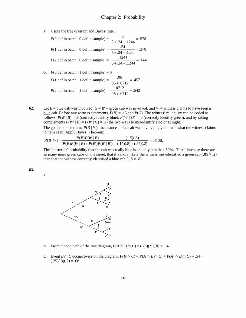
Chapter 2: Probability
70
a. Using the tree diagram and Bayes’ rule,
P(0 def in batch | 0 def in sample) = 578.1244.24.5.
5.=
++
P(1 def in batch | 0 def in sample) = 278.1244.24.5.
24.=
++
P(2 def in batch | 0 def in sample) = 144.1244.24.5.
1244.=
++
b. P(0 def in batch | 1 def in sample) = 0
P(1 def in batch | 1 def in sample) = 457.0712.06.
06.=
+
P(2 def in batch | 1 def in sample) = 543.0712.06.
0712.=
+
62. Let B = blue cab was involved, G = B′ = green cab was involved, and W = witness claims to have seen a
blue cab. Before any witness statements, P(B) = .15 and P(G). The witness’ reliability can be coded as follows: P(W | B) = .8 (correctly identify blue), P(W′ | G) = .8 (correctly identify green), and by taking complements P(W′ | B) = P(W | G) = .2 (the two ways to mis-identify a color at night). The goal is to determine P(B | W), the chance a blue cab was involved given that’s what the witness claims to have seen. Apply Bayes’ Theorem:
( ) ( | ) (.15)(.8)( | )( ) ( | ) ( ) ( | ) (.15)(.8) (.85)(.2)
P B P W BP B WP B P W B P B P W B
= =′ ′+ +
= .4138.
The “posterior” probability that the cab was really blue is actually less than 50%. That’s because there are so many more green cabs on the street, that it’s more likely the witness mis-identified a green cab (.85 × .2) than that the witness correctly identified a blue cab (.15 × .8).
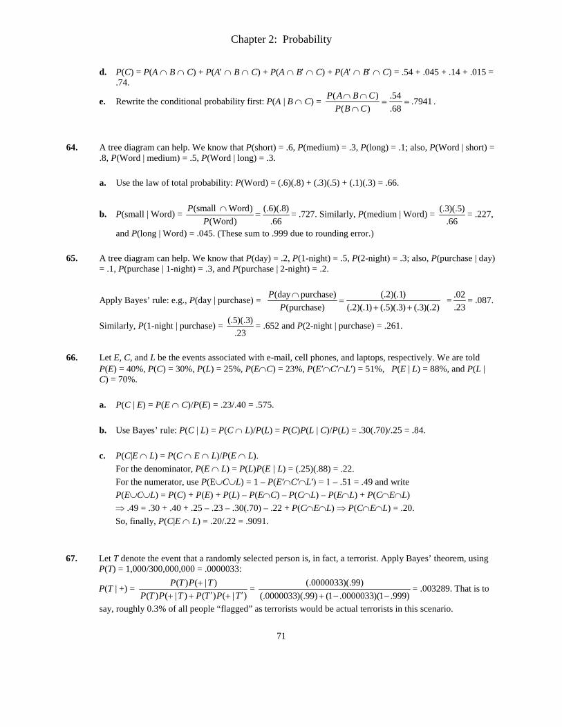
63. a.
b. From the top path of the tree diagram, P(A ∩ B ∩ C) = (.75)(.9)(.8) = .54. c. Event B ∩ C occurs twice on the diagram: P(B ∩ C) = P(A ∩ B ∩ C) + P(A′ ∩ B ∩ C) = .54 +
(.25)(.8)(.7) = .68.
Chapter 2: Probability
71
d. P(C) = P(A ∩ B ∩ C) + P(A′ ∩ B ∩ C) + P(A ∩ B′ ∩ C) + P(A′ ∩ B′ ∩ C) = .54 + .045 + .14 + .015 = .74.
e. Rewrite the conditional probability first: P(A | B ∩ C) = 7941.68.54.
)()(
==∩∩∩CBP
CBAP .
64. A tree diagram can help. We know that P(short) = .6, P(medium) = .3, P(long) = .1; also, P(Word | short) = .8, P(Word | medium) = .5, P(Word | long) = .3.
a. Use the law of total probability: P(Word) = (.6)(.8) + (.3)(.5) + (.1)(.3) = .66.
b. P(small | Word) = (small Word) (.6)(.8)(Word) .66
PP
∩= = .727. Similarly, P(medium | Word) = (.3)(.5)
.66= .227,
and P(long | Word) = .045. (These sum to .999 due to rounding error.)
65. A tree diagram can help. We know that P(day) = .2, P(1-night) = .5, P(2-night) = .3; also, P(purchase | day) = .1, P(purchase | 1-night) = .3, and P(purchase | 2-night) = .2.
Apply Bayes’ rule: e.g., P(day | purchase) = (day purchase) (.2)(.1)(purchase) (.2)(.1) (.5)(.3) (.3)(.2)
PP
∩=
+ + = .02
.23= .087.
Similarly, P(1-night | purchase) = (.5)(.3).23
= .652 and P(2-night | purchase) = .261.
66. Let E, C, and L be the events associated with e-mail, cell phones, and laptops, respectively. We are told
P(E) = 40%, P(C) = 30%, P(L) = 25%, P(E∩C) = 23%, P(E′∩C′∩L′) = 51%, P(E | L) = 88%, and P(L | C) = 70%.
a. P(C | E) = P(E ∩ C)/P(E) = .23/.40 = .575. b. Use Bayes’ rule: P(C | L) = P(C ∩ L)/P(L) = P(C)P(L | C)/P(L) = .30(.70)/.25 = .84. c. P(C|E ∩ L) = P(C ∩ E ∩ L)/P(E ∩ L).
For the denominator, P(E ∩ L) = P(L)P(E | L) = (.25)(.88) = .22. For the numerator, use P(E∪C∪L) = 1 – P(E′∩C′∩L′) = 1 – .51 = .49 and write P(E∪C∪L) = P(C) + P(E) + P(L) – P(E∩C) – P(C∩L) – P(E∩L) + P(C∩E∩L) ⇒ .49 = .30 + .40 + .25 – .23 – .30(.70) – .22 + P(C∩E∩L) ⇒ P(C∩E∩L) = .20. So, finally, P(C|E ∩ L) = .20/.22 = .9091.
67. Let T denote the event that a randomly selected person is, in fact, a terrorist. Apply Bayes’ theorem, using
P(T) = 1,000/300,000,000 = .0000033:
P(T | +) = ( ) ( | )( ) ( | ) ( ) ( | )
P T P TP T P T P T P T
+′ ′+ + +
= )999.1)(0000033.1()99)(.0000033(.
)99)(.0000033(.−−+
= .003289. That is to
say, roughly 0.3% of all people “flagged” as terrorists would be actual terrorists in this scenario.
Chapter 2: Probability
72
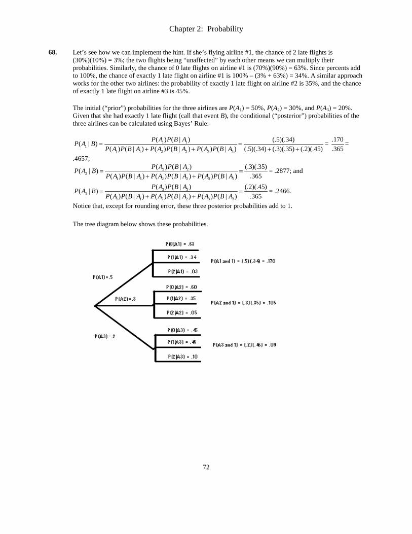
68. Let’s see how we can implement the hint. If she’s flying airline #1, the chance of 2 late flights is (30%)(10%) = 3%; the two flights being “unaffected” by each other means we can multiply their probabilities. Similarly, the chance of 0 late flights on airline #1 is (70%)(90%) = 63%. Since percents add to 100%, the chance of exactly 1 late flight on airline #1 is 100% – (3% + 63%) = 34%. A similar approach works for the other two airlines: the probability of exactly 1 late flight on airline #2 is 35%, and the chance of exactly 1 late flight on airline #3 is 45%. The initial (“prior”) probabilities for the three airlines are P(A1) = 50%, P(A2) = 30%, and P(A3) = 20%. Given that she had exactly 1 late flight (call that event B), the conditional (“posterior”) probabilities of the three airlines can be calculated using Bayes’ Rule:
2 2 3
1 11
1 1 3
( ) ( | ) (.5)(.34)| )( ) ( | ) ( ) ( | ) ( ) ( | ) (.5)(.34) (.3)(.35) (.2)(.45)
( P A P B ABP A P B A P A P B A P A P
P AB A
= =+ + + +
= .170.365
=
.4657; 2 2
22 31 321
( ) ( | ) (.3)(.35)| )( ) ( | ) ( ) ( | ) ( ) ( | ) .3 5
(6
P A P B ABP A P B A P A P B A P A P
P AB A
= =+ +
= .2877; and
3 33
2 31 321
( ) ( | ) (.2)(.45)| )( ) ( | ) ( ) ( | ) ( ) ( | ) .3 5
(6
P A P B ABP A P B A P A P B A P A P
P AB A
= =+ +
= .2466.
Notice that, except for rounding error, these three posterior probabilities add to 1. The tree diagram below shows these probabilities.
Chapter 2: Probability
73
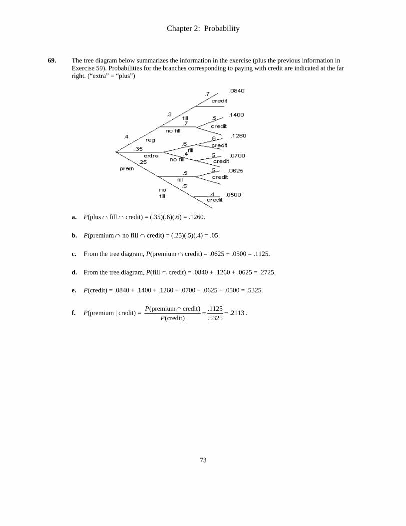
69. The tree diagram below summarizes the information in the exercise (plus the previous information in
Exercise 59). Probabilities for the branches corresponding to paying with credit are indicated at the far right. (“extra” = “plus”)
a. P(plus ∩ fill ∩ credit) = (.35)(.6)(.6) = .1260. b. P(premium ∩ no fill ∩ credit) = (.25)(.5)(.4) = .05. c. From the tree diagram, P(premium ∩ credit) = .0625 + .0500 = .1125. d. From the tree diagram, P(fill ∩ credit) = .0840 + .1260 + .0625 = .2725. e. P(credit) = .0840 + .1400 + .1260 + .0700 + .0625 + .0500 = .5325.
f. P(premium | credit) = (premium credit) .1125 .2113(credit) .5325
PP
∩= = .
Chapter 2: Probability
74
Section 2.5 70. Using the definition, two events A and B are independent if P(A | B) = P(A);
P(A | B) = .6125; P(A) = .50; .6125 ≠ .50, so A and B are not independent. Using the multiplication rule, the events are independent if P(A ∩ B)=P(A)P(B); P(A ∩ B) = .25; P(A)P(B) = (.5)(.4) = .2. .25 ≠ .2, so A and B are not independent.
71.
a. Since the events are independent, then A′ and B′ are independent, too. (See the paragraph below Equation 2.7.) Thus, P(B′|A′) = P(B′) = 1 – .7 = .3.
b. Using the addition rule, P(A ∪ B) = P(A) + P(B) – P(A ∩ B) =.4 + .7 – (.4)(.7) = .82. Since A and B are
independent, we are permitted to write P(A ∩ B) = P(A)P(B) = (.4)(.7).
c. P(AB′ | A ∪ B) = ( ( )) ( ( ) ( ) (.4)(1 .7) .12 .146( ) ( )
)( ) .8 .822
P A PP AB A B P ABP A B
BP AP A B B
′ ′∩ ∪= = = = =
∪′
∪∪− .
72. P(A1 ∩ A2) = .11 while P(A1)P(A2) = .055, so A1 and A2 are not independent.
P(A1 ∩ A3) = .05 while P(A1)P(A3) = .0616, so A1 and A3 are not independent. P(A2 ∩ A3) = .07 and P(A2)P(A3) = .07, so A2 and A3 are independent.
73. From a Venn diagram, P(B) = P(A′ ∩ B) + P(A ∩ B) = P(B) ⇒ P(A′ ∩ B) = P(B) – P(A ∩ B). If A and B
are independent, then P(A′ ∩ B) = P(B) – P(A)P(B) = [1 – P(A)]P(B) = P(A′)P(B). Thus, A′ and B are independent.
Alternatively, ( ) ( ) ( )( | )( ) ( )
P A B P B P A BP A BP B P B′∩ − ∩′ = = = ( ) ( ) ( )
( )P B P A P B
P B−
= 1 – P(A) = P(A′).
74. Using subscripts to differentiate between the selected individuals,
P(O1 ∩ O2) = P(O1)P(O2) = (.45)(.45) = .2025. P(two individuals match) = P(A1 ∩ A2) + P(B1 ∩ B2) + P(AB1 ∩ AB2) + P(O1∩O2) = .402 + .112 + .042 + .452 = .3762.
75. Let event E be the event that an error was signaled incorrectly.
We want P(at least one signaled incorrectly) = P(E1 ∪ … ∪ E10). To use independence, we need intersections, so apply deMorgan’s law: = P(E1 ∪ …∪ E10) = 1 – 1 10 )(P EE ′∩ ∩′
. P(E′) = 1 – .05 = .95, so for 10 independent points, 1 10 )(P EE ′∩ ∩′
= (.95)…(.95) = (.95)10. Finally, P(E1 ∪ E2 ∪ …∪ E10) = 1 – (.95)10 = .401. Similarly, for 25 points, the desired probability is 1 – (P(E′))25 = 1 – (.95)25 = .723.
Chapter 2: Probability
75
76. Follow the same logic as in Exercise 75: If the probability of an event is p, and there are n independent “trials,” the chance this event never occurs is (1 – p)n, while the chance of at least one occurrence is 1 – (1 – p)n. With p = 1/9,000,000,000 and n = 1,000,000,000, this calculates to 1 – .9048 = .0952. Note: For extremely small values of p, (1 – p)n ≈ 1 – np. So, the probability of at least one occurrence under these assumptions is roughly 1 – (1 – np) = np. Here, that would equal 1/9.
77. Let p denote the probability that a rivet is defective.
a. .15 = P(seam needs reworking) = 1 – P(seam doesn’t need reworking) = 1 – P(no rivets are defective) = 1 – P(1st isn’t def ∩ … ∩ 25th isn’t def) = 1 – (1 – p)…(1 – p) = 1 – (1 – p)25. Solve for p: (1 – p)25 = .85 ⇒ 1 – p = (.85)1/25 ⇒ p = 1 – .99352 = .00648.
b. The desired condition is .10 = 1 – (1 – p)25. Again, solve for p: (1 – p)25 = .90 ⇒
p = 1 – (.90)1/25 = 1 – .99579 = .00421. 78. P(at least one opens) = 1 – P(none open) = 1 – (.04)5 = .999999897.
P(at least one fails to open) = 1 – P(all open) = 1 – (.96)5 = .1846. 79. Let A1 = older pump fails, A2 = newer pump fails, and x = P(A1 ∩ A2). The goal is to find x. From the Venn
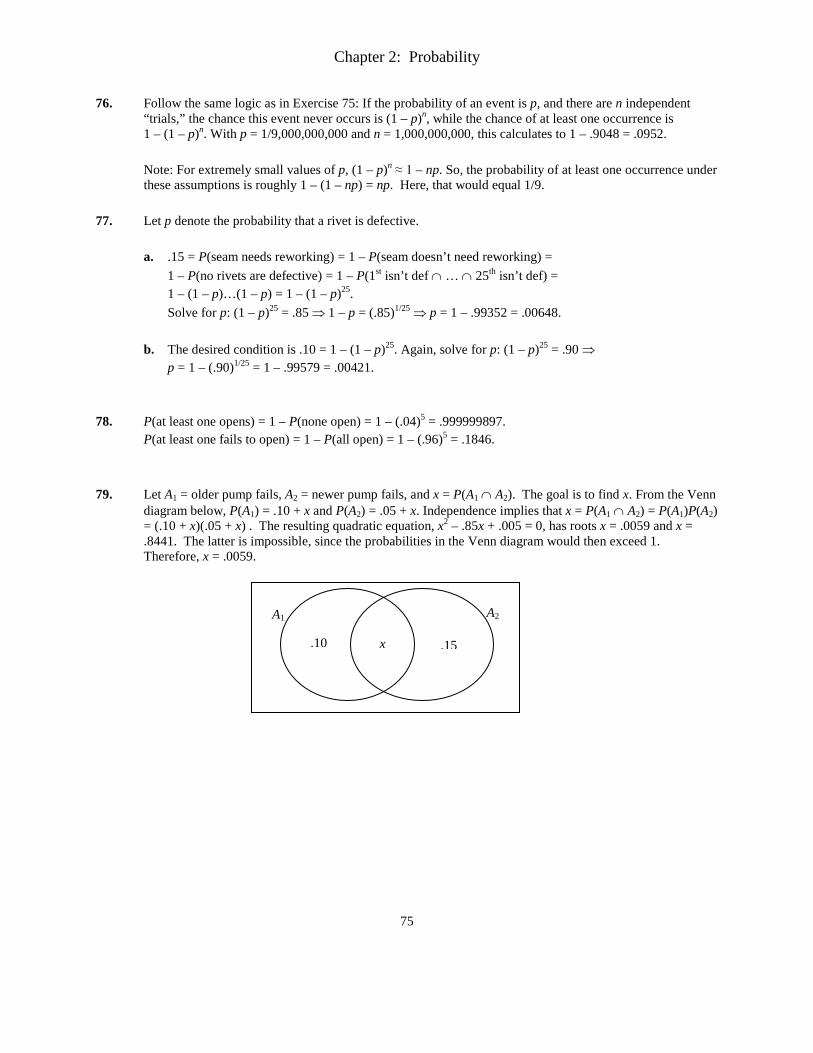
diagram below, P(A1) = .10 + x and P(A2) = .05 + x. Independence implies that x = P(A1 ∩ A2) = P(A1)P(A2) = (.10 + x)(.05 + x) . The resulting quadratic equation, x2 – .85x + .005 = 0, has roots x = .0059 and x = .8441. The latter is impossible, since the probabilities in the Venn diagram would then exceed 1. Therefore, x = .0059.
.10 .15 x
A1 A2
Chapter 2: Probability
76
80. Let Ai denote the event that component #i works (i = 1, 2, 3, 4). Based on the design of the system, the
event “the system works” is 1 2 3 4) ( )( A A AA ∪ ∪ ∩ . We’ll eventually need 1 2 )(P A A∪ , so work that out first: 1 2 1 2 1 2) ( ) ( ) ( ) (.9) (.9) (.9)(.9 .( ) 99A P A P A P A AP A ∪ = + − ∩ = + − = . The third term uses independence of events. Also, 3 4( )P A A∩ = (.8)(.8) = .64, again using independence.
Now use the addition rule and independence for the system:
1 2 3 4 1 2 3 4 1 2 3 4
1 2 3 4 1 2 3 4
) ( )) ( ) ( ) ) ( ))( ) ( ) ) ( )
(.99) (.64) (.99)(.6
(( ((
4) .9964(
A A A P A P A A A A AP A P A A
P A A P AA AP P AA A
∪ ∪ ∩ = ∪ + ∩ − ∪ ∩ ∩= ∪ + ∩ − ∪ × ∩= + − =
(You could also use deMorgan’s law in a couple of places.) 81. Using the hints, let P(Ai) = p, and x = p2. Following the solution provided in the example,
P(system lifetime exceeds t0) = p2 + p2 – p4 = 2p2 – p4 = 2x – x2. Now, set this equal to .99: 2x – x2 = .99 ⇒ x2 – 2x + .99 = 0 ⇒ x = 0.9 or 1.1 ⇒ p = 1.049 or .9487. Since the value we want is a probability and cannot exceed 1, the correct answer is p = .9487.
82. A = {(3,1)(3,2)(3,3)(3,4)(3,5)(3,6)} ⇒ P(A) = 6
3616= ; B = {(1,4)(2,4)(3,4)(4,4)(5,4)(6,4)} ⇒ P(B) = 6
1 ;
and C = {(1,6)(2,5)(3,4)(4,3)(5,2)(6,1)} ⇒ P(C) = 61 .
A∩B = {(3,4)} ⇒ P(A∩B) = 361 = P(A)P(B); A∩C = {(3,4)} ⇒ P(A∩C) = 36
1 = P(A)P(C); and B∩C =
{(3,4)} ⇒ P(B∩C) = 361 = P(B)P(C). Therefore, these three events are pairwise independent.
However, A∩B∩C = {(3,4)} ⇒ P(A∩B∩C) = 361 , while P(A)P(B)P(C) = =
1 1 1 16 6 6 216⋅ ⋅ = , so P(A∩B∩C) ≠
P(A)P(B)P(C) and these three events are not mutually independent. 83. We’ll need to know P(both detect the defect) = 1 – P(at least one doesn’t) = 1 – .2 = .8.
a. P(1st detects ∩ 2nd doesn’t) = P(1st detects) – P(1st does ∩ 2nd does) = .9 – .8 = .1. Similarly, P(1st doesn’t ∩ 2nd does) = .1, so P(exactly one does)= .1 + .1= .2.
b. P(neither detects a defect) = 1 – [P(both do) + P(exactly 1 does)] = 1 – [.8+.2] = 0. That is, under this model there is a 0% probability neither inspector detects a defect. As a result, P(all 3 escape) = (0)(0)(0) = 0.
Chapter 2: Probability
77
84. We’ll make repeated use of the independence of the Ais and their complements. a. 1 2 3 1 2 3) ( ) ( ) ( )( A A P A P AA P AP ∩ ∩ = = (.95)(.98)(.80) = .7448.
b. This is the complement of part a, so the answer is 1 – .7448 = .2552. c. 1 2 3 1 2 3) ( ) ( ) (( )A A P A P A P AP A ′ ′ ′ ′ ′∩ ∩ =′ = (.05)(.02)(.20) = .0002.
d. 1 2 3 1 2 3) ( ) ( ( )( )A A P A P A PA AP ′ ′∩ ∩ = = (.05)(.98)(.80) = .0392.
e. 1 2 3 1 2 3 1 2 3] ] ])([ [ [A A AP A A AA A A′ ′∩ ∩ ∪ ∩ ∩ ∪ ∩ ∩′ = (.05)(.98)(.80) + (.95)(.02)(.80) + (.95)(.98)(.20)
= .07302. f. This is just a little joke — we’ve all had the experience of electronics dying right after the warranty
expires! 85.
a. Let D1 = detection on 1st fixation, D2 = detection on 2nd fixation. P(detection in at most 2 fixations) = P(D1) + 1 2( )P D D′∩ ; since the fixations are independent,
P(D1) + 1 2( )P D D′∩ = P(D1) + 1( )P D′ P(D2) = p + (1 – p)p = p(2 – p).
b. Define D1, D2, … , Dn as in a. Then P(at most n fixations) = P(D1) + 1 2( )P D D′∩ + 1 2 3( )D DP D′∩ ∩′ + … + 1 2 1( )n nP D D DD −′ ′∩ ∩ ∩ ∩′
= p + (1 – p)p + (1 – p)2p + … + (1 – p)n–1p = p[1 + (1 – p) + (1 – p)2 + … + (1 – p)n–1] =
1 (1 ) 1 (1 )1 (1 )
·n
npp pp
− −= − −
− −.
Alternatively, P(at most n fixations) = 1 – P(at least n+1 fixations are required) = 1 – P(no detection in 1st n fixations) = 1 – 1 2 )( nD DP D ′ ′∩ ∩ ∩′
= 1 – (1 – p)n.
c. P(no detection in 3 fixations) = (1 – p)3.
d. P(passes inspection) = P({not flawed} ∪ {flawed and passes}) = P(not flawed) + P(flawed and passes) = .9 + P(flawed) P(passes | flawed) = .9 + (.1)(1 – p)3.
e. Borrowing from d, P(flawed | passed) = 3
3
(flawed passed) .1(1 )(passed) .9 .1(1 )
P pP p
∩ −=
+ −. For p = .5,
P(flawed | passed) = 3
3
.1(1 .5) .0137.9 .1(1 .5)
−=
+ −.
Chapter 2: Probability
78
86.
a. P(A) = 2,00010,000
= .2. Using the law of total probability, ( ) ( ) ( | ) ( ) ( | )P B P A P B A P A P B A′ ′= + =
1,999 2,000(.2) (.8)9,999 9,999
+ = .2 exactly. That is, P(B) = P(A) = .2. Finally, use the multiplication rule:
1,999) ( ) ( | ) (.2)9,999
( B P A P B AP A∩ = × = = .039984. Events A and B are not independent, since P(B) =
.2 while 1,999| ) .199929 999
(,
P B A = = , and these are not equal.
b. If A and B were independent, we’d have ) ( ) ( ) (.2)(.2) .0( 4B P A P BP A∩ = × = = . This is very close to
the answer .039984 from part a. This suggests that, for most practical purposes, we could treat events A and B in this example as if they were independent.
c. Repeating the steps in part a, you again get P(A) = P(B) = .2. However, using the multiplication rule,
2 1) ( ) ( | )10
(9
B P A P B AP A∩ = × = × =.0222. This is very different from the value of .04 that we’d get
if A and B were independent!
The critical difference is that the population size in parts a-b is huge, and so the probability a second board is green almost equals .2 (i.e., 1,999/9,999 = .19992 ≈ .2). But in part c, the conditional probability of a green board shifts a lot: 2/10 = .2, but 1/9 = .1111.
87. a. Use the information provided and the addition rule:
P(A1 ∪ A2) = P(A1) + P(A2) – P(A1 ∩ A2) ⇒ P(A1 ∩ A2) = P(A1) + P(A2) – P(A1 ∪ A2) = .55 + .65 – .80 = .40.
b. By definition, 2 32 3
3
( ) .40( |( ) .70
) P A AAP A
P A ∩== = .5714. If a person likes vehicle #3, there’s a 57.14%
chance s/he will also like vehicle #2.
c. No. From b, 2 3( )|P A A = .5714 ≠ P(A2) = .65. Therefore, A2 and A3 are not independent. Alternatively, P(A2 ∩ A3) = .40 ≠ P(A2)P(A3) = (.65)(.70) = .455.
d. The goal is to find 2 3 1| )( AP A A′∪ , i.e. 2 3 1
1
([ ] )( )A AP A
P A′∪ ∩
′. The denominator is simply 1 – .55 = .45.
There are several ways to calculate the numerator; the simplest approach using the information provided is to draw a Venn diagram and observe that 2 3 1 1 2 3 1) (([ (] ) )A A P A A PA A AP ′∪ ∩ = ∪ ∪ − =
.88 – .55 = .33. Hence, 2 3 1| )( AP A A′∪ = .33.45
= .7333.
Chapter 2: Probability
79
88. Let D = patient has disease, so P(D) = .05. Let ++ denote the event that the patient gets two independent,
positive tests. Given the sensitivity and specificity of the test, P(++ | D) = (.98)(.98) = .9604, while P(++ | D′) = (1 – .99)(1 – .99) = .0001. (That is, there’s a 1-in-10,000 chance of a healthy person being mis-diagnosed with the disease twice.) Apply Bayes’ Theorem:
( ) ( | ) (.05)(.9604)( | )( ) ( | ) ( ) ( | ) (.05)(.9604) (.95)(.0001)
P D P DP DP D P D P D P D
++++ = =
′ ′++ + ++ + = .9980
89. The question asks for P(exactly one tag lost | at most one tag lost) = 1 2 1 2 1 2((( ) ))) | (C C CC CP C′ ′∩ ∪ ∩ ∩ ′ . Since the first event is contained in (a subset of) the second event, this equals
1 2 1 2
1 2
(( ))(
( )( )
)C CC
P CP
CC
′∩ ∪ ∩′∩
′= 1 2 1 2 1 2 1 2
1 2 1 2
( ( (1
) ( ) ) ( ) ) ( )) ( )( 1 ) (
P P CC C P C C P C P CP CP C P CC P C
′=
− −′ ′ ′∩ + ∩ +
∩by independence =
2 21(1 ) (1 ) 2 (1 ) 2
1 1π π π π π π π
π π π=
−−
=−+ −
+− .
Chapter 2: Probability
80
Supplementary Exercises 90.
a. 103
= 120.
b. There are 9 other senators from whom to choose the other two subcommittee members, so the answer
is 1 × 92
= 36.
c. There are 120 possible subcommittees. Among those, the number which would include none of the 5
most senior senators (i.e., all 3 members are chosen from the 5 most junior senators) is 53
= 10.
Hence, the number of subcommittees with at least one senior senator is 120 – 10 = 110, and the chance of this randomly occurring is 110/120 = .9167.
d. The number of subcommittees that can form from the 8 “other” senators is 83
= 56, so the
probability of this event is 56/120 = .4667.
91.
a. P(line 1) = 5001500
= .333;
P(crack) = ( ) ( ) ( ).50 500 .44 400 .40 600 6661500 1500
+ += = .444.
b. This is one of the percentages provided: P(blemish | line 1) = .15.
c. P(surface defect) = ( ) ( ) ( ).10 500 .08 400 .15 600 1721500 1500
+ += ;
P(line 1 ∩ surface defect) = ( ).10 500 501500 1500
= ;
so, P(line 1 | surface defect) = 50 /1500172 /
51 00 25
017
= = .291.
92.
a. He will have one type of form left if either 4 withdrawals or 4 course substitutions remain. This means the first six were either 2 withdrawals and 4 subs or 6 withdrawals and 0 subs; the desired probability
is 6 4 62 4 6
1
40
06
+
= 16210
=.0762.
Chapter 2: Probability
81
b. He can start with the withdrawal forms or the course substitution forms, allowing two sequences: W-C-
W-C or C-W-C-W. The number of ways the first sequence could arise is (6)(4)(5)(3) = 360, and the number of ways the second sequence could arise is (4)(6)(3)(5) = 360, for a total of 720 such possibilities. The total number of ways he could select four forms one at a time is P4,10 = (10)(9)(8)(7) = 5040. So, the probability of a perfectly alternating sequence is 720/5040 = .143.
93. Apply the addition rule: P(A∪B) = P(A) + P(B) – P(A ∩ B) ⇒ .626 = P(A) + P(B) – .144. Apply
independence: P(A ∩ B) = P(A)P(B) = .144. So, P(A) + P(B) = .770 and P(A)P(B) = .144. Let x = P(A) and y = P(B). Using the first equation, y = .77 – x, and substituting this into the second equation yields x(.77 – x) = .144 or x2 – .77x + .144 = 0. Use the quadratic formula to solve:
x =2.77 ( .77) (4)(1)(.144) .77 .13
2(1) 2± − − ±
= = .32 or .45. Since x = P(A) is assumed to be the larger
probability, x = P(A) = .45 and y = P(B) = .32.
94. The probability of a bit reversal is .2, so the probability of maintaining a bit is .8.
a. Using independence, P(all three relays correctly send 1) = (.8)(.8)(.8) = .512. b. In the accompanying tree diagram, each .2 indicates a bit reversal (and each .8 its opposite). There are
several paths that maintain the original bit: no reversals or exactly two reversals (e.g., 1 → 1 → 0 → 1, which has reversals at relays 2 and 3). The total probability of these options is .512 + (.8)(.2)(.2) + (.2)(.8)(.2) + (.2)(.2)(.8) = .512 + 3(.032) = .608.
c. Using the answer from b, P(1 sent | 1 received) = 1 received)(1 sent(1 received)
PP
∩ =
(1 received | 1 sent)(1 received | 1 sent)
(1 sent)(1 sent) (0 se (1 received n | 0 sen )t) t
PPP P
PP+
= (.7)(.608) .4256(.7)(.608) (.3)(.392) .5432
=+
=
.7835. In the denominator, P(1 received | 0 sent) = 1 – P(0 received | 0 sent) = 1 – .608, since the answer from b also applies to a 0 being relayed as a 0.
Chapter 2: Probability
82
95. a. There are 5! = 120 possible orderings, so P(BCDEF) = 1
120 = .0833. b. The number of orderings in which F is third equals 4×3×1*×2×1 = 24 (*because F must be here), so
P(F is third) = 24120 = .2. Or more simply, since the five friends are ordered completely at random, there
is a ⅕ chance F is specifically in position three.
c. Similarly, P(F last) = 4 3 2 1 1120
× × × × = .2.
d. P(F hasn’t heard after 10 times) = P(not on #1 ∩ not on #2 ∩ … ∩ not on #10) = 104 4
5 545
× × =
=
.1074.
96. Palmberg equation: ( / *)( )1 ( / *)d
c ccc c
Pβ
β=+
a. ( * / *) 1 1( *) .51 ( * / *) 1 1 1 1d
c ccc c
Pβ β
β β= = = =+ + +
.
b. The probability of detecting a crack that is twice the size of the “50-50” size c* equals
(2 * / *) 2(2 *)1 (2 * / *) 1 2dP c cc
c c
β β
β β= =+ +
. When β = 4, 4
4
2 16(2 *)1 2 17dP c = =+
= .9412.
c. Using the answers from a and b, P(exactly one of two detected) = P(first is, second isn’t) + P(first
isn’t, second is) = (.5)(1 – .9412) + (1 – .5)(.9412) = .5.
d. If c = c*, then Pd(c) = .5 irrespective of β. If c < c*, then c/c* < 1 and Pd(c) → 00 1+
= 0 as β → ∞.
Finally, if c > c* then c/c* > 1 and, from calculus, Pd(c) → 1 as β → ∞. 97. When three experiments are performed, there are 3 different ways in which detection can occur on exactly
2 of the experiments: (i) #1 and #2 and not #3; (ii) #1 and not #2 and #3; and (iii) not #1 and #2 and #3. If the impurity is present, the probability of exactly 2 detections in three (independent) experiments is (.8)(.8)(.2) + (.8)(.2)(.8) + (.2)(.8)(.8) = .384. If the impurity is absent, the analogous probability is 3(.1)(.1)(.9) = .027. Thus, applying Bayes’ theorem, P(impurity is present | detected in exactly 2 out of 3)
= (detected in exactly 2 present)(detected in exactly 2)
PP
∩ = (.384)(.4)(.384)(.4) (.027)(.6)+
= .905.
Chapter 2: Probability
83
98. Our goal is to find P(A ∪ B ∪ C ∪ D ∪ E). We’ll need all of the following probabilities:
P(A) = P(Allison gets her calculator back) = 1/5. This is intuitively obvious; you can also see it by writing out the 5! = 120 orderings in which the friends could get calculators (ABCDE, ABCED, …, EDCBA) and observe that 24 of the 120 have A in the first position. So, P(A) = 24/120 = 1/5. By the same reasoning, P(B) = P(C) = P(D) = P(E) = 1/5. P(A ∩ B) = P(Allison and Beth get their calculators back) = 1/20. This can be computed by considering all 120 orderings and noticing that six — those of the form ABxyz — have A and B in the correct positions. Or, you can use the multiplication rule: P(A ∩ B) = P(A)P(B | A) = (1/5)(1/4) = 1/20. All other pairwise intersection probabilities are also 1/20. P(A ∩ B ∩ C) = P(Allison and Beth and Carol get their calculators back) = 1/60, since this can only occur if two ways — ABCDE and ABCED — and 2/120 = 1/60. So, all three-wise intersections have probability 1/60. P(A ∩ B ∩ C ∩ D) = 1/120, since this can only occur if all 5 girls get their own calculators back. In fact, all four-wise intersections have probability 1/120, as does P(A ∩ B ∩ C ∩ D ∩ E) — they’re the same event. Finally, put all the parts together, using a general inclusion-exclusion rule for unions:
) ( ) ( ) ( ) ( ) ( )( ) ( ) ( )( ) ( )( ) ( )( )1 1 1 1 1 1 1 1 1 765 10 10
(
5 1 .6335 20 60 120 2 6120 120 24 1 02
B C D E P A P B P C P D P EP A B P A C P D EP A B C P C D EP A B C D P B C D EP A B C D E
P A∪ ∪ ∪ ∪ = + + + +− ∩ − ∩ − − ∩+ ∩ ∩ + + ∩ ∩− ∩ ∩ ∩ − − ∩ ∩ ∩+ ∩ ∩ ∩ ∩
= ⋅ − ⋅ + ⋅ − ⋅ + = − + − + = =
The final answer has the form 1 1 1 1 1 1 1 12 6 24 1! 2! 3! 4! 5!
1 + − = − + − +− . Generalizing to n friends, the
probability at least one will get her own calculator back is 11 1 1 1 1( 1)1! 2! 3! 4! !
n
n−− + − + + − .
When n is large, we can relate this to the power series for ex evaluated at x = –1:
0
2 3
1
1
1! 2! 3!1 1 1 1 1 111! 2! 3! 1! 2! 3!
1 1 111! 2!
1!
1
3!
x
k
kx x x
e
ek
x
e
∞
=
−
−
+ + + ⇒
+ − + = − − + − ⇒
− =
= =
− +
+
= −
−
∑
So, for large n, P(at least one friend gets her own calculator back) ≈ 1 – e–1 = .632. Contrary to intuition, the chance of this event does not converge to 1 (because “someone is bound to get hers back”) or to 0 (because “there are just too many possible arrangements”). Rather, in a large group, there’s about a 63.2% chance someone will get her own item back (a match), and about a 36.8% chance that nobody will get her own item back (no match).
Chapter 2: Probability
84
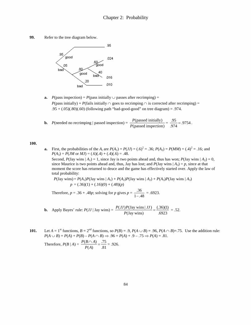
99. Refer to the tree diagram below.
a. P(pass inspection) = P(pass initially ∪ passes after recrimping) =
P(pass initially) + P(fails initially ∩ goes to recrimping ∩ is corrected after recrimping) = .95 + (.05)(.80)(.60) (following path “bad-good-good” on tree diagram) = .974.
b. P(needed no recrimping | passed inspection) = (passed initially)(passed inspection)P
P= .95 .9754
.974= .
100.
a. First, the probabilities of the Ai are P(A1) = P(JJ) = (.6)2 = .36; P(A2) = P(MM) = (.4)2 = .16; and P(A3) = P(JM or MJ) = (.6)(.4) + (.4)(.6) = .48. Second, P(Jay wins | A1) = 1, since Jay is two points ahead and, thus has won; P(Jay wins | A2) = 0, since Maurice is two points ahead and, thus, Jay has lost; and P(Jay wins | A3) = p, since at that moment the score has returned to deuce and the game has effectively started over. Apply the law of total probability: P(Jay wins) = P(A1)P(Jay wins | A1) + P(A2)P(Jay wins | A2) + P(A3)P(Jay wins | A3) p = (.36)(1) + (.16)(0) + (.48)(p)
Therefore, p = .36 + .48p; solving for p gives p = .361 .48−
= .6923.
b. Apply Bayes’ rule: P(JJ | Jay wins) = ( ) (Jay wins | )(Jay wins)
(.36)(1).6923
P JJ P JJP
= = .52.
101. Let A = 1st functions, B = 2nd functions, so P(B) = .9, P(A ∪ B) = .96, P(A ∩ B)=.75. Use the addition rule:
P(A ∪ B) = P(A) + P(B) – P(A ∩ B) ⇒ .96 = P(A) + .9 – .75 ⇒ P(A) = .81.
Therefore, P(B | A) = ( ) .75( ) .81
P B AP A∩
= = .926.
Chapter 2: Probability
85
102.
a. P(F) = 919/2026 = .4536. P(C) = 308/2026 = .1520.
b. P(F ∩ C) = 110/2026 = .0543. Since P(F) × P(C) = .4536 × .1520 = .0690 ≠ .0543, we find that events F and C are not independent.
c. P(F | C) = P(F ∩ C)/P(C) = 110/308 = .3571.
d. P(C | F) = P(C ∩ F)/P(F) = 110/919 = .1197.
e. Divide each of the two rows, Male and Female, by its row total. Blue Brown Green Hazel Male .3342 .3180 .1789 .1689 Female .3906 .3156 .1197 .1741 According to the data, brown and hazel eyes have similar likelihoods for males and females. However, females are much more likely to have blue eyes than males (39% versus 33%) and, conversely, males have a much greater propensity for green eyes than do females (18% versus 12%).
103. A tree diagram can help here.
a. P(E1 ∩ L) = P(E1)P(L | E1) = (.40)(.02) = .008.
b. The law of total probability gives P(L) = ∑ P(Ei)P(L | Ei) = (.40)(.02) + (.50)(.01) + (.10)(.05) = .018.
c. 1 1| ) 1 ( )( |L P LP E E′ ′=′ − = 1 )(1( )
P EP L
L′′∩
− = 1 1) |(1 ( )
( )1 P L EP EP L
′−
−= (.40)(.98)1
1 .018−
−= .601.
104. Let B denote the event that a component needs rework. By the law of total probability,
P(B) = ∑ P(Ai)P(B | Ai) = (.50)(.05) + (.30)(.08) + (.20)(.10) = .069.
Thus, P(A1 | B) = (.50)(.05).069
= .362, P(A2 | B) = (.30)(.08).069
= .348, and P(A3 | B) = .290.
105. This is the famous “Birthday Problem” in probability.
a. There are 36510 possible lists of birthdays, e.g. (Dec 10, Sep 27, Apr 1, …). Among those, the number with zero matching birthdays is P10,365 (sampling ten birthdays without replacement from 365 days. So,
P(all different) = 1010,365
10
(365)(364) (356)365 (365)P
= = .883. P(at least two the same) = 1 – .883 = .117.
Chapter 2: Probability
86
b. The general formula is P(at least two the same) = 1 – ,365
365k
k
P. By trial and error, this probability equals
.476 for k = 22 and equals .507 for k = 23. Therefore, the smallest k for which k people have at least a 50-50 chance of a birthday match is 23.
c. There are 1000 possible 3-digit sequences to end a SS number (000 through 999). Using the idea from
a, P(at least two have the same SS ending) = 1 – 10,1000101000
P= 1 – .956 = .044.
Assuming birthdays and SS endings are independent, P(at least one “coincidence”) = P(birthday coincidence ∪ SS coincidence) = .117 + .044 – (.117)(.044) = .156.
Chapter 2: Probability
87
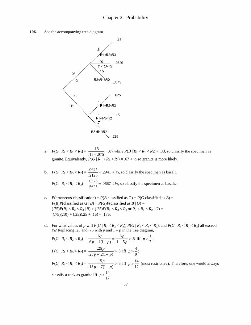
106. See the accompanying tree diagram.
a. P(G | R1 < R2 < R3) = .15 .67.15 .075
=+
while P(B | R1 < R2 < R3) = .33, so classify the specimen as
granite. Equivalently, P(G | R1 < R2 < R3) = .67 > ½ so granite is more likely.
b. P(G | R1 < R3 < R2) = .0625 .2941.2125
= < ½, so classify the specimen as basalt.
P(G | R3 < R1 < R2) = .0375 .0667.5625
= < ½, so classify the specimen as basalt.
c. P(erroneous classification) = P(B classified as G) + P(G classified as B) =
P(B)P(classified as G | B) + P(G)P(classified as B | G) = (.75)P(R1 < R2 < R3 | B) + (.25)P(R1 < R3 < R2 or R3 < R1 < R2 | G) = (.75)(.10) + (.25)(.25 + .15) = .175.
d. For what values of p will P(G | R1 < R2 < R3), P(G | R1 < R3 < R2), and P(G | R3 < R1 < R2) all exceed ½? Replacing .25 and .75 with p and 1 – p in the tree diagram,
P(G | R1 < R2 < R3) = .6 .6 .5.6 .1(1 ) .1 .5
p pp p p
= >+ − +
iff 17
p > ;
P(G | R1 < R3 < R2) = .25 .5.25 .2(1 )
pp p
>+ −
iff 49
p > ;
P(G | R3 < R1 < R2) = .15 .5.15 .7(1 )
pp p
>+ −
iff 1417
p > (most restrictive). Therefore, one would always
classify a rock as granite iff 1417
p > .
Chapter 2: Probability
88
107. P(detection by the end of the nth glimpse) = 1 – P(not detected in first n glimpses) =
1 – 1 2 )( nG GP G ′ ′∩ ∩ ∩′ = 1 – 1 2) ( )( ( ) nP GP G P G′ ′ ′
= 1 – (1 – p1)(1 – p2) … (1 – pn) = 1 – )1(1 i
n
ip−Π
=.
108.
a. P(walks on 4th pitch) = P(first 4 pitches are balls) = (.5)4 = .0625. b. P(walks on 6th pitch) = P(2 of the first 5 are strikes ∩ #6 is a ball) =
P(2 of the first 5 are strikes)P(#6 is a ball) = 52
(.5)2(.5)3 (.5) = .15625.
c. Following the pattern from b, P(walks on 5th pitch) = 41
(.5)1(.5)3(.5) = .125. Therefore, P(batter
walks) = P(walks on 4th) + P(walks on 5th) + P(walks on 6th) = .0625 + .125 + .15625 = .34375.
d. P(first batter scores while no one is out) = P(first four batters all walk) = (.34375)4 = .014. 109.
a. P(all in correct room) = 1 14! 24= = .0417.
b. The 9 outcomes which yield completely incorrect assignments are: 2143, 2341, 2413, 3142, 3412,
3421, 4123, 4321, and 4312, so P(all incorrect) = 924
= .375.
110.
a. P(all full) = P(A ∩ B ∩ C) = (.9)(.7)(.8) = .504. P(at least one isn’t full) = 1 – P(all full) = 1 – .504 = .496.
b. P(only NY is full) = P(A ∩ B′ ∩ C′) = P(A)P(B′)P(C′) = (.9)(1–.7)(1–.8) = .054. Similarly, P(only Atlanta is full) = .014 and P(only LA is full) = .024. So, P(exactly one full) = .054 + .014 + .024 = .092.
Chapter 2: Probability
89
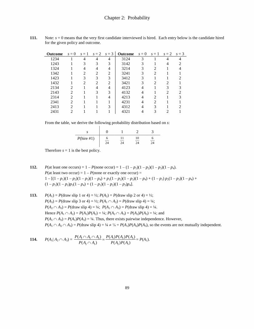
111. Note: s = 0 means that the very first candidate interviewed is hired. Each entry below is the candidate hired
for the given policy and outcome.
Outcome s = 0 s = 1 s = 2 s = 3 Outcome s = 0 s = 1 s = 2 s = 3 1234 1 4 4 4 3124 3 1 4 4 1243 1 3 3 3 3142 3 1 4 2 1324 1 4 4 4 3214 3 2 1 4 1342 1 2 2 2 3241 3 2 1 1 1423 1 3 3 3 3412 3 1 1 2 1432 1 2 2 2 3421 3 2 2 1 2134 2 1 4 4 4123 4 1 3 3 2143 2 1 3 3 4132 4 1 2 2 2314 2 1 1 4 4213 4 2 1 3 2341 2 1 1 1 4231 4 2 1 1 2413 2 1 1 3 4312 4 3 1 2 2431 2 1 1 1 4321 4 3 2 1
From the table, we derive the following probability distribution based on s:
s 0 1 2 3 P(hire #1)
246
2411
2410
246
Therefore s = 1 is the best policy. 112. P(at least one occurs) = 1 – P(none occur) = 1 – (1 – p1)(1 – p2)(1 – p3)(1 – p4).
P(at least two occur) = 1 – P(none or exactly one occur) = 1 – [(1 – p1)(1 – p2)(1 – p3)(1 – p4) + p1(1 – p2)(1 – p3)(1 – p4) + (1 – p1) p2(1 – p3)(1 – p4) + (1 – p1)(1 – p2)p3(1 – p4) + (1 – p1)(1 – p2)(1 – p3)p4].
113. P(A1) = P(draw slip 1 or 4) = ½; P(A2) = P(draw slip 2 or 4) = ½; P(A3) = P(draw slip 3 or 4) = ½; P(A1 ∩ A2) = P(draw slip 4) = ¼; P(A2 ∩ A3) = P(draw slip 4) = ¼; P(A1 ∩ A3) = P(draw slip 4) = ¼. Hence P(A1 ∩ A2) = P(A1)P(A2) = ¼; P(A2 ∩ A3) = P(A2)P(A3) = ¼; and P(A1 ∩ A3) = P(A1)P(A3) = ¼. Thus, there exists pairwise independence. However, P(A1 ∩ A2 ∩ A3) = P(draw slip 4) = ¼ ≠ ⅛ = P(A1)P(A2)P(A3), so the events are not mutually independent.
114. P(A1| A2 ∩ A3) = 1 2 3 1 2 3
2 3 2 3
( ) ( ) ( ) ( )( ) ( ) ( )
P A A A P A P A P AP A A P A P A∩ ∩
=∩
= P(A1).

Copyright © Cengage Learning. All rights reserved.
Probability

Copyright © Cengage Learning. All rights reserved.
2.5 Independence
3
Independence
The definition of conditional probability enables us to revise the probability P(A) originally assigned to A when we are subsequently informed that another event B has occurred; the new probability of A is P(A | B).
In our examples, it was frequently the case that P(A | B) differed from the unconditional probability P(A), indicating that the information “B has occurred” resulted in a change in the chance of A occurring.
Often the chance that A will occur or has occurred is not affected by knowledge that B has occurred, so that P(A | B) = P(A).
4
Independence
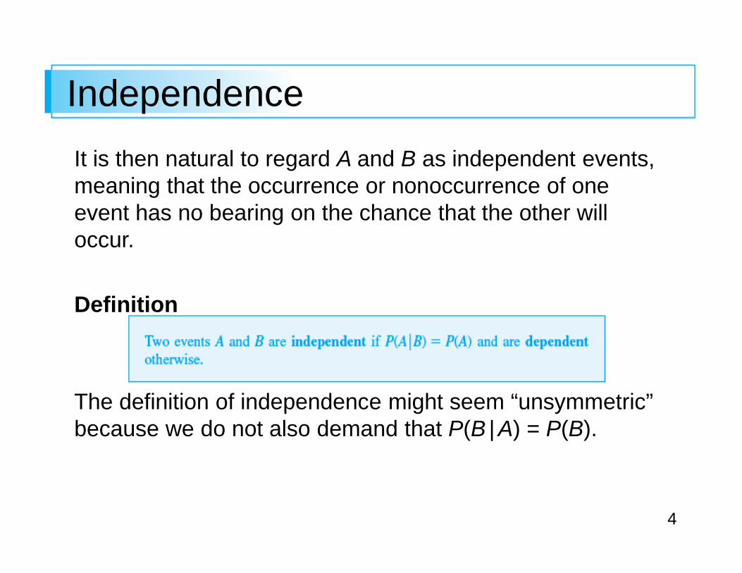
It is then natural to regard A and B as independent events, meaning that the occurrence or nonoccurrence of one event has no bearing on the chance that the other will occur.
Definition
The definition of independence might seem “unsymmetric” because we do not also demand that P(B | A) = P(B).
5
Independence
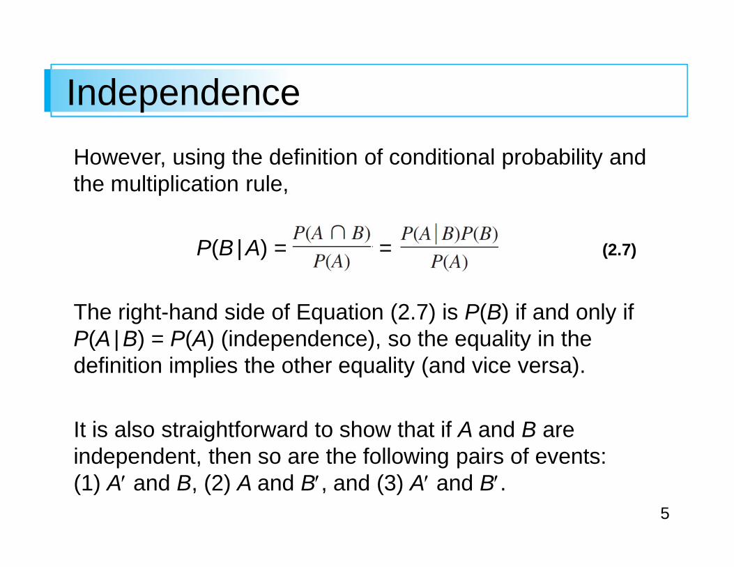
However, using the definition of conditional probability and the multiplication rule,
P(B | A) = = (2.7)
The right-hand side of Equation (2.7) is P(B) if and only if P(A | B) = P(A) (independence), so the equality in the definition implies the other equality (and vice versa).
It is also straightforward to show that if A and B are independent, then so are the following pairs of events: (1) A′ and B, (2) A and B′, and (3) A′ and B′.
6
Example 2.32
Consider a gas station with six pumps numbered 1, 2, . . . , 6, and let Ei denote the simple event that a randomly selected customer uses pump i (i = 1, . . . ,6).
Suppose thatP(E1) = P(E6) = .10,
P(E2) = P(E5) = .15,
P(E3) = P(E4) = .25
Define events A, B, C by
A = {2, 4, 6}, B = {1, 2, 3}, C = {2, 3, 4, 5}.
7
Example 2.32
We then have P(A) = .50, P(A | B) = .30, and P(A | C) = .50. That is, events A and B are dependent, whereas events A and C are independent.
Intuitively, A and C are independent because the relative division of probability among even- and odd-numbered pumps is the same among pumps 2, 3, 4, 5 as it is among all six pumps.
cont’d

8
The Multiplication Rule for P(A ∩ B)
9
The Multiplication Rule for P(A ∩ B)
Frequently the nature of an experiment suggests that two events A and B should be assumed independent.
This is the case, for example, if a manufacturer receives a circuit board from each of two different suppliers, each board is tested on arrival, and
A = {first is defective} and
B = {second is defective}.
10
The Multiplication Rule for P(A ∩ B)
If P(A) = .1, it should also be the case that P(A | B) = .1; knowing the condition of the second board shouldn’t provide information about the condition of the first.
The probability that both events will occur is easily calculated from the individual event probabilities when the events are independent.
11
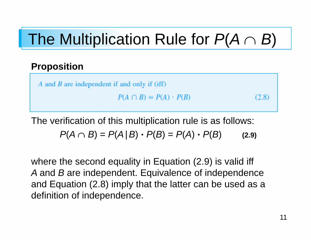
The Multiplication Rule for P(A ∩ B)
Proposition
The verification of this multiplication rule is as follows:
P(A ∩ B) = P(A | B) P(B) = P(A) P(B) (2.9)
where the second equality in Equation (2.9) is valid iff A and B are independent. Equivalence of independence and Equation (2.8) imply that the latter can be used as a definition of independence.
12
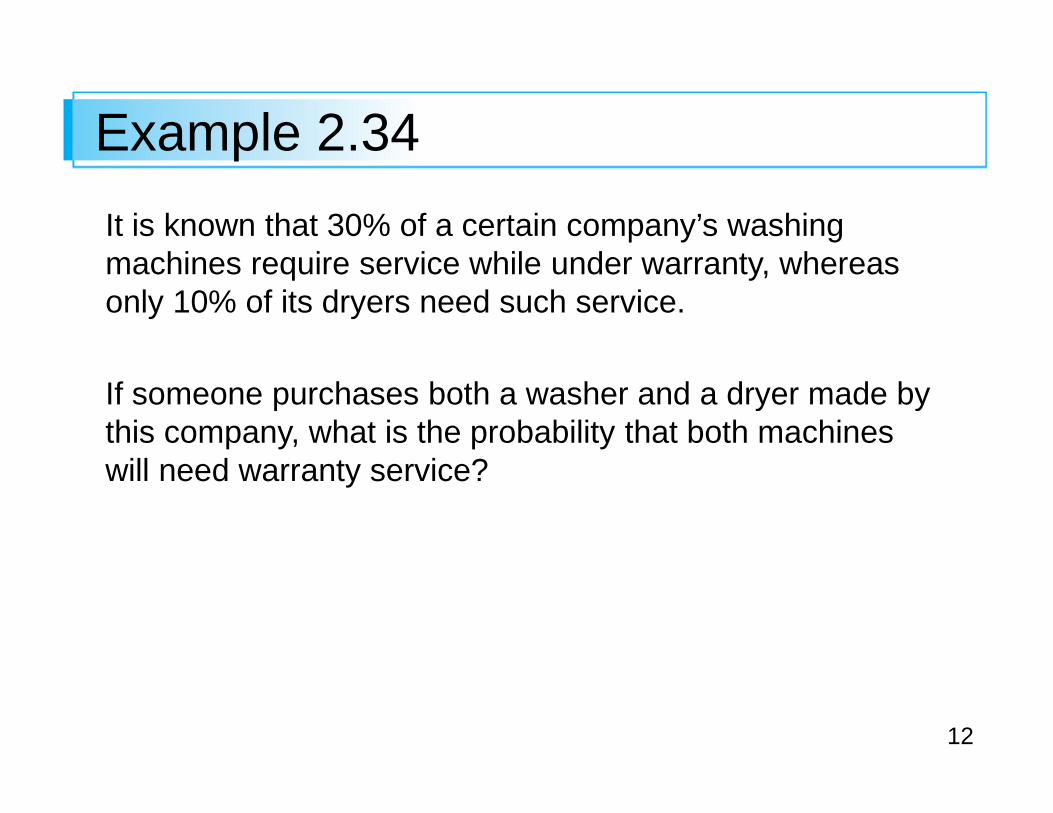
Example 2.34
It is known that 30% of a certain company’s washing machines require service while under warranty, whereas only 10% of its dryers need such service.
If someone purchases both a washer and a dryer made by this company, what is the probability that both machines will need warranty service?
13
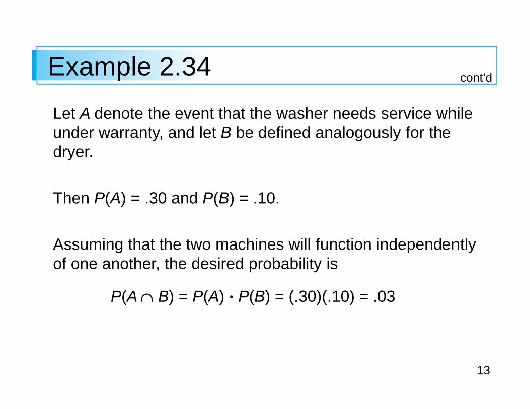
Example 2.34
Let A denote the event that the washer needs service while under warranty, and let B be defined analogously for the dryer.
Then P(A) = .30 and P(B) = .10.
Assuming that the two machines will function independently of one another, the desired probability is
P(A ∩ B) = P(A) P(B) = (.30)(.10) = .03
cont’d

14
Independence of More Than Two Events
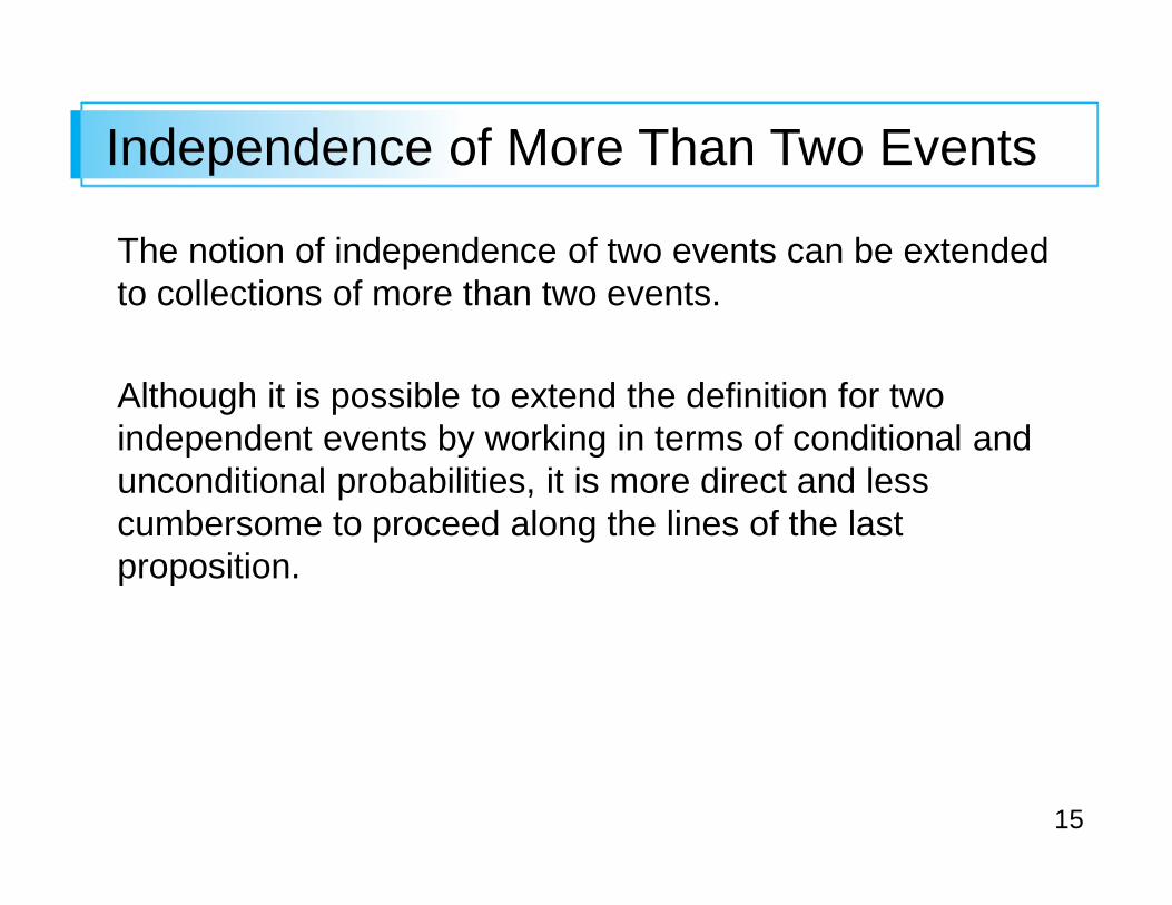
15
Independence of More Than Two Events
The notion of independence of two events can be extended to collections of more than two events.
Although it is possible to extend the definition for two independent events by working in terms of conditional and unconditional probabilities, it is more direct and less cumbersome to proceed along the lines of the last proposition.
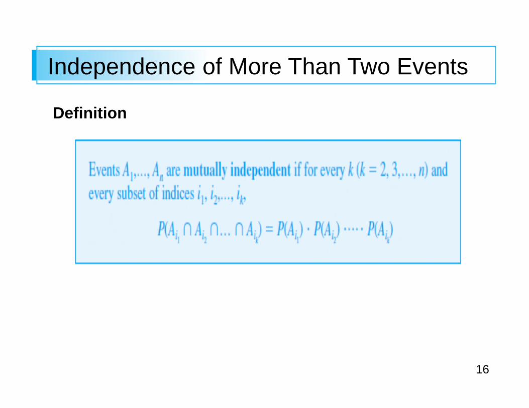
16
Independence of More Than Two Events
Definition
17
Independence of More Than Two Events
To paraphrase the definition, the events are mutually independent if the probability of the intersection of any subset of the n events is equal to the product of the individual probabilities.
In using the multiplication property for more than two independent events, it is legitimate to replace one or more of the Ais by their complements (e.g., if A1, A2, and A3 are independent events, so are and ).
18
Independence of More Than Two Events
As was the case with two events, we frequently specify at the outset of a problem the independence of certain events.
The probability of an intersection can then be calculated via multiplication.
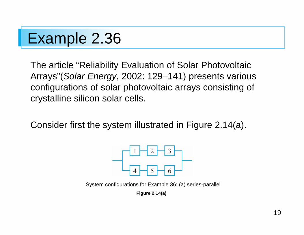
19
Example 2.36
The article “Reliability Evaluation of Solar Photovoltaic Arrays”(Solar Energy, 2002: 129–141) presents various configurations of solar photovoltaic arrays consisting of crystalline silicon solar cells.
Consider first the system illustrated in Figure 2.14(a).
Figure 2.14(a)
System configurations for Example 36: (a) series-parallel
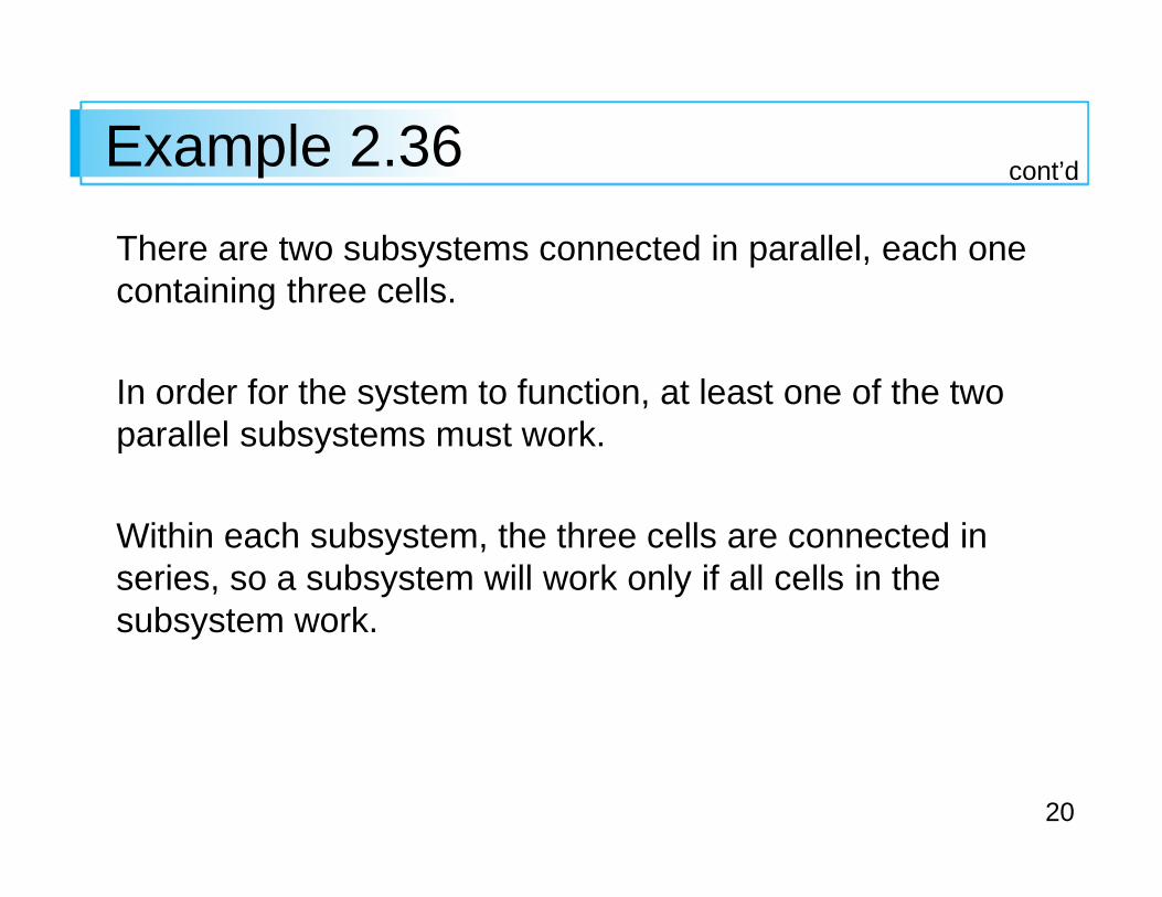
20
Example 2.36
There are two subsystems connected in parallel, each one containing three cells.
In order for the system to function, at least one of the two parallel subsystems must work.
Within each subsystem, the three cells are connected in series, so a subsystem will work only if all cells in the subsystem work.
cont’d
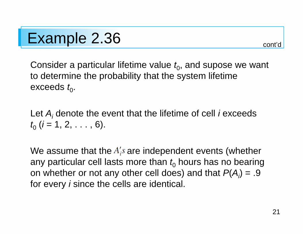
21
Example 2.36
Consider a particular lifetime value t0, and supose we want to determine the probability that the system lifetime exceeds t0.
Let Ai denote the event that the lifetime of cell i exceedst0 (i = 1, 2, . . . , 6).
We assume that the are independent events (whether any particular cell lasts more than t0 hours has no bearing on whether or not any other cell does) and that P(Ai) = .9 for every i since the cells are identical.
cont’d
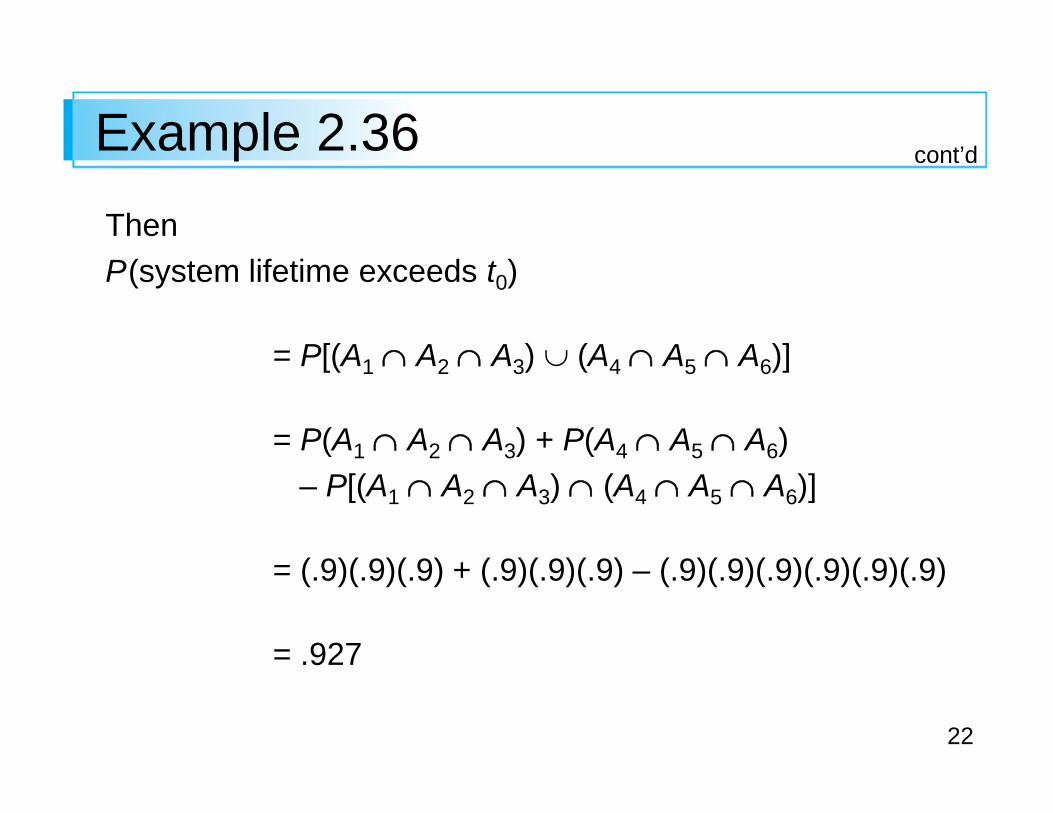
22
Example 2.36
Then
P(system lifetime exceeds t0)
= P[(A1 ∩ A2 ∩ A3) ∪ (A4 ∩ A5 ∩ A6)]
= P(A1 ∩ A2 ∩ A3) + P(A4 ∩ A5 ∩ A6)
– P[(A1 ∩ A2 ∩ A3) ∩ (A4 ∩ A5 ∩ A6)]
= (.9)(.9)(.9) + (.9)(.9)(.9) – (.9)(.9)(.9)(.9)(.9)(.9)
= .927
cont’d
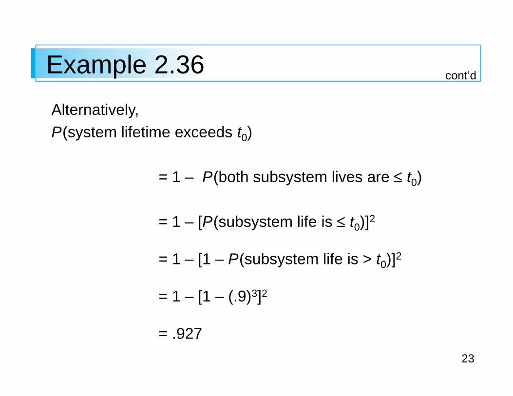
23
Example 2.36
Alternatively,
P(system lifetime exceeds t0)
= 1 – P(both subsystem lives are ≤ t0)
= 1 – [P(subsystem life is ≤ t0)]2
= 1 – [1 – P(subsystem life is > t0)]2
= 1 – [1 – (.9)3]2
= .927
cont’d
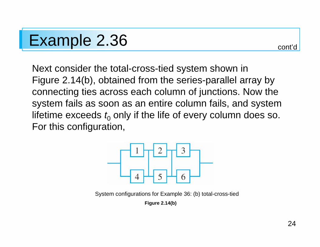
24
Example 2.36
Next consider the total-cross-tied system shown in Figure 2.14(b), obtained from the series-parallel array by connecting ties across each column of junctions. Now the system fails as soon as an entire column fails, and system lifetime exceeds t0 only if the life of every column does so. For this configuration,
Figure 2.14(b)
System configurations for Example 36: (b) total-cross-tied
cont’d
25
Example 2.36
P(system lifetime is at least t0)
= [P(column lifetime exceeds t0)]3
= [1 – P(column lifetime ≤ t0)]3
= [1 – P(both cells in a column have lifetime ≤ t0)]3
= [1 – (1 – .9)2]3
= .970
cont’d

Copyright © Cengage Learning. All rights reserved.
Probability

Copyright © Cengage Learning. All rights reserved.
2.1 Sample Spaces and Events
3
Sample Spaces and Events
An experiment is any activity or process whose outcome is subject to uncertainty.
Although the word experiment generally suggests a planned or carefully controlled laboratory testing situation, we use it here in a much wider sense.
Thus experiments that may be of interest include tossing a coin once or several times, selecting a card or cards from a deck, weighing a loaf of bread, ascertaining the commuting time from home to work on a particular morning, obtaining blood types from a group of individuals, or measuring the compressive strengths of different steel beams.

4
The Sample Space of an Experiment
5
The Sample Space of an Experiment
Definition
6
Example 2.1
The simplest experiment to which probability applies is one with two possible outcomes.
One such experiment consists of examining a single weld to see whether it is defective.
The sample space for this experiment can be abbreviated as = {N, D}, where N represents not defective, D represents defective, and the braces are used toenclose the elements of a set.
7
Example 2.1
Another such experiment would involve tossing a thumbtack and noting whether it landed point up or point down, with sample space = {U, D}, and yet another would consist of observing the gender of the next child born at the local hospital, with = {M, F}.
cont’d

8
Events
9
Events
In our study of probability, we will be interested not only in the individual outcomes of but also in various collections of outcomes from .
Definition
10
Events
When an experiment is performed, a particular event A is said to occur if the resulting experimental outcome is contained in A.
In general, exactly one simple event will occur, but many compound events will occur simultaneously.
11
Example 2.5
Consider an experiment in which each of three vehicles taking a particular freeway exit turns left (L) or right (R) at the end of the exit ramp.
The eight possible outcomes that comprise the sample space are LLL, RLL, LRL, LLR, LRR, RLR, RRL, and RRR.
Thus there are eight simple events, among which are E1 = {LLL} and E5 = {LRR}.
12
Example 2.5
Some compound events include
A = {LLL, LRL, LLR} = the event that exactly one of the
three vehicles turns right
B = {LLL, RLL, LRL, LLR} = the event that at most one of the vehicles turns right
C = {LLL, RRR} = the event that all three vehicles turn in the same direction
cont’d
13
Example 2.5
Suppose that when the experiment is performed, the outcome is LLL.
Then the simple event E1 has occurred and so also have the events B and C (but not A).
cont’d
14
Some Relations from Set Theory
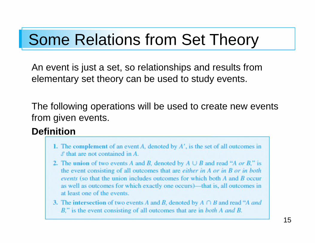
15
Some Relations from Set Theory
An event is just a set, so relationships and results from elementary set theory can be used to study events.
The following operations will be used to create new events from given events.
Definition
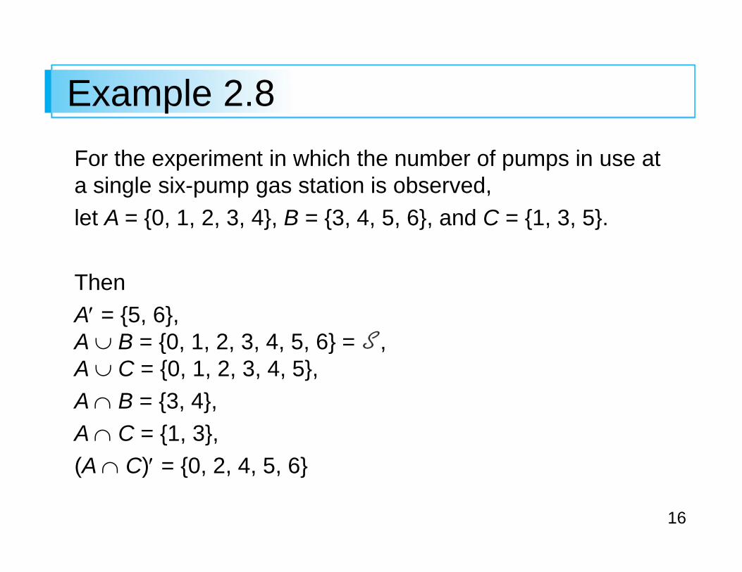
16
Example 2.8
For the experiment in which the number of pumps in use at a single six-pump gas station is observed,
let A = {0, 1, 2, 3, 4}, B = {3, 4, 5, 6}, and C = {1, 3, 5}.
Then
A′ = {5, 6}, A ∪ B = {0, 1, 2, 3, 4, 5, 6} = ,A ∪ C = {0, 1, 2, 3, 4, 5},
A ∩ B = {3, 4},
A ∩ C = {1, 3},
(A ∩ C)′ = {0, 2, 4, 5, 6}
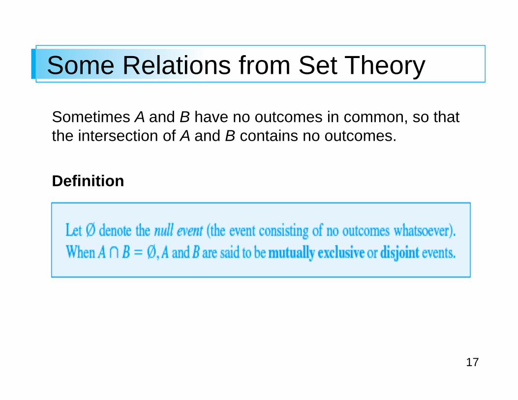
17
Some Relations from Set Theory
Sometimes A and B have no outcomes in common, so that the intersection of A and B contains no outcomes.
Definition
18
Example 2.10
A small city has three automobile dealerships: a GM dealer selling Chevrolets and Buicks; a Ford dealer selling Fords and Lincolns; and a Toyota dealer.
If an experiment consists of observing the brand of the next car sold, then the events A = {Chevrolet, Buick} and B = {Ford, Lincoln} are mutually exclusive becausethe next car sold cannot be both a GM product and a Ford product (at least until the two companies merge!).
19
Some Relations from Set Theory
The operations of union and intersection can be extended to more than two events.
For any three events A, B, and C, the event A ∪ B ∪ C is the set of outcomes contained in at least one of the three events, whereas A ∩ B ∩ C is the set of outcomes contained in all three events.
Given events A1, A2, A3 ,..., these events are said to be mutually exclusive (or pairwise disjoint) if no two events have any outcomes in common.
20
Some Relations from Set Theory
A pictorial representation of events and manipulations with events is obtained by using Venn diagrams.
To construct a Venn diagram, draw a rectangle whose interior will represent the sample space .
Then any event A is represented as the interior of a closedcurve (often a circle) contained in .
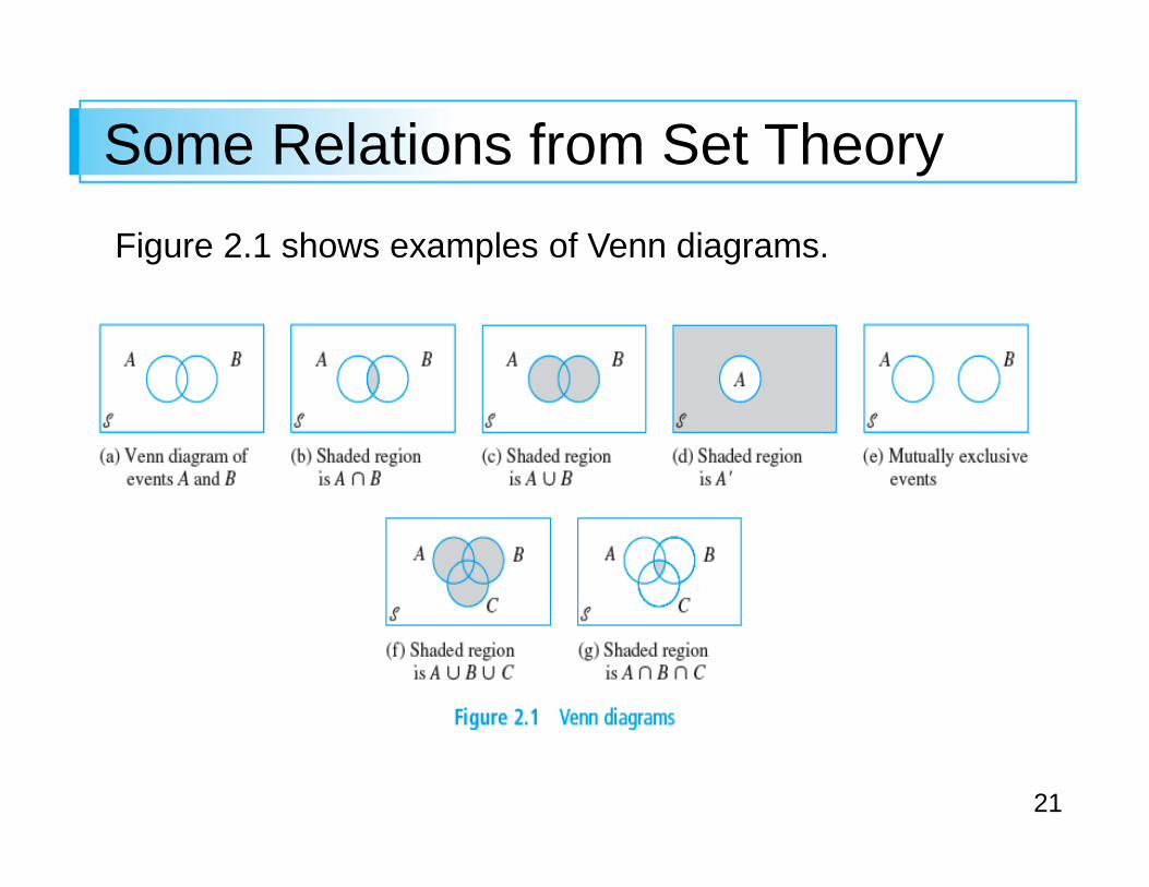
21
Some Relations from Set Theory
Figure 2.1 shows examples of Venn diagrams.

Copyright © Cengage Learning. All rights reserved.
Probability
Copyright © Cengage Learning. All rights reserved.
2.2Axioms, Interpretations,
and Properties of Probability
3
Axioms, Interpretations, and Properties of Probability
Given an experiment and a sample space , the objective of probability is to assign to each event A a number P(A),called the probability of the event A, which will give a precise measure of the chance that A will occur.
To ensure that the probability assignments will be consistent with our intuitive notions of probability, all assignments should satisfy the following axioms (basic properties) of probability.
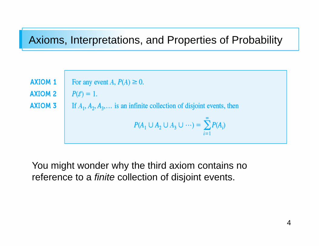
4
Axioms, Interpretations, and Properties of Probability
You might wonder why the third axiom contains no reference to a finite collection of disjoint events.
5
Axioms, Interpretations, and Properties of Probability
It is because the corresponding property for a finitecollection can be derived from our three axioms. We want our axiom list to be as short as possible and not contain any property that can be derived from others on the list.
Axiom 1 reflects the intuitive notion that the chance of A occurring should be nonnegative.
The sample space is by definition the event that must occur when the experiment is performed ( contains all possible outcomes), so Axiom 2 says that the maximum possible probability of 1 is assigned to .
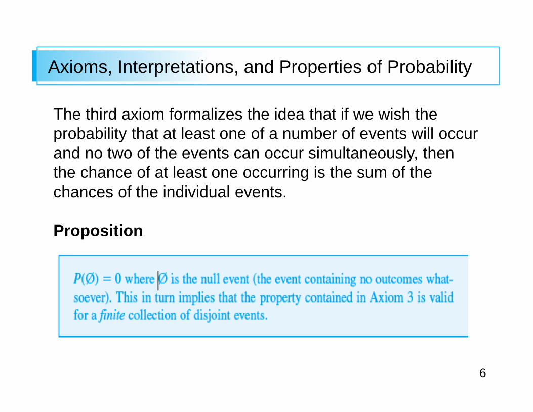
6
Axioms, Interpretations, and Properties of Probability
The third axiom formalizes the idea that if we wish the probability that at least one of a number of events will occurand no two of the events can occur simultaneously, then the chance of at least one occurring is the sum of the chances of the individual events.
Proposition
7
Example 2.11
Consider tossing a thumbtack in the air. When it comes to rest on the ground, either its point will be up (the outcome U) or down (the outcome D). The sample space for this event is therefore = {U, D}.
The axioms specify P( ) = 1, so the probability assignment will be completed by determining P(U) and P(D).
Since U and D are disjoint and their union is , the foregoing proposition implies that
1 = P( ) = P(U) + P(D)
8
Example 2.11
It follows that P(D) = 1 – P(U).
One possible assignment of probabilities is
P(U) = .5, P(D) = .5,
whereas another possible assignment is
P(U) = .75, P(D) = .25.
In fact, letting p represent any fixed number between 0 and 1, P(U) = p, P(D) = 1 – p is an assignment consistent with the axioms.
cont’d
9
Example 2.12
Consider testing batteries coming off an assembly line one by one until one having a voltage within prescribed limits is found.
The simple events are
E1 = {S}, E2 = {FS},
E3 = {FFS}, E4 = {FFFS}, . . . .
Suppose the probability of any particular battery being satisfactory is .99.
10
Example 2.12
Then it can be shown that
P(E1) = .99, P(E2) = (.01)(.99),
P(E3) = (.01)2(.99), . . . is an assignment of probabilities to the simple events that satisfies the axioms. In particular, because the Eis are disjoint and = E1 ∪ E2 ∪ E3 ∪…,it must be the case that
1 = P(S) = P(E1) + P(E2) + P(E3) + ···
= .99[1 + .01 + (.01)2 + (.01)3 + ···]
cont’d
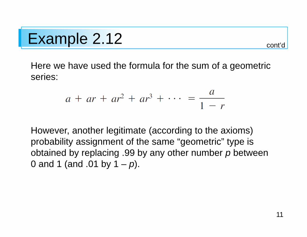
11
Example 2.12
Here we have used the formula for the sum of a geometric series:
However, another legitimate (according to the axioms) probability assignment of the same “geometric” type is obtained by replacing .99 by any other number p between 0 and 1 (and .01 by 1 – p).
cont’d
12
Interpreting Probability
13
Interpreting Probability
Examples 2.11 and 2.12 show that the axioms do not completely determine an assignment of probabilities to events. The axioms serve only to rule out assignments inconsistent with our intuitive notions of probability.
In the tack-tossing experiment of Example 2.11, two particular assignments were suggested.
The appropriate or correct assignment depends on the nature of the thumbtack and also on one’s interpretation of probability.
14
Interpreting Probability
The interpretation that is most frequently used and most easily understood is based on the notion of relative frequencies.
Consider an experiment that can be repeatedly performed in an identical and independent fashion, and let A be an event consisting of a fixed set of outcomes of the experiment.
Simple examples of such repeatable experiments include the tacktossing and die-tossing experiments previously discussed.
15
Interpreting Probability
If the experiment is performed n times, on some of the replications the event A will occur (the outcome will be in the set A), and on others, A will not occur.
Let n(A) denote the number of replications on which A does occur.
Then the ratio n(A)/n is called the relative frequency of occurrence of the event A in the sequence of n replications.
16
Interpreting Probability
For example, let A be the event that a package sent within the state of California for 2nd day delivery actually arrives within one day.
The results from sending 10 such packages (the first 10 replications) are as follows:
17
Interpreting Probability
Figure 2.2(a) shows how the relative frequency n(A)/nfluctuates rather substantially over the course of the first 50 replications.
Figure 2.2
Behavior of relative frequency (a) Initial fluctuation
18
Interpreting Probability
But as the number of replications continues to increase, Figure 2.2(b) illustrates how the relative frequency stabilizes.
Figure 2.2
Behavior of relative frequency (b) Long-run stabilization
19
Interpreting Probability
More generally, empirical evidence, based on the results of many such repeatable experiments, indicates that any relative frequency of this sort will stabilize as the number of replications n increases.
That is, as n gets arbitrarily large, n(A)/n approaches a limiting value referred to as the limiting (or long-run) relative frequency of the event A.
The objective interpretation of probability identifies this limiting relative frequency with P(A).
20
Interpreting Probability
Suppose that probabilities are assigned to events in accordance with their limiting relative frequencies.
Then a statement such as “the probability of a package being delivered within one day of mailing is .6” means that of a large number of mailed packages, roughly 60% will arrive within one day.
Similarly, if B is the event that an appliance of a particular type will need service while under warranty, then P(B) = .1 is interpreted to mean that in the long run 10% of such appliances will need warranty service.
21
Interpreting Probability
This doesn’t mean that exactly 1 out of 10 will need service, or that exactly 10 out of 100 will need service, because 10 and 100 are not the long run.
This relative frequency interpretation of probability is said to be objective because it rests on a property of the experiment rather than on any particular individual concerned with the experiment.
For example, two different observers of a sequence of coin tosses should both use the same probability assignments since the observers have nothing to do with limiting relative frequency.
22
Interpreting Probability
In practice, this interpretation is not as objective as it might seem, since the limiting relative frequency of an event will not be known.
Thus we will have to assign probabilities based on our beliefs about the limiting relative frequency of events under study.
Fortunately, there are many experiments for which there will be a consensus with respect to probability assignments.
23
Interpreting Probability
When we speak of a fair coin, we shall mean
P(H) = P(T) = .5,
and a fair die is one for which limiting relative frequencies
of the six outcomes are all suggesting probability
assignments P({1}) = · · · = P({6}) =
Because the objective interpretation of probability is based on the notion of limiting frequency, its applicability is limited to experimental situations that are repeatable.
24
Interpreting Probability
Yet the language of probability is often used in connection with situations that are inherently unrepeatable.
Examples include: “The chances are good for a peace agreement”; “It is likely that our company will be awarded the contract”; and “Because their best quarterback is injured, I expect them to score no more than 10 points against us.”
In such situations we would like, as before, to assign numerical probabilities to various outcomes and events (e.g., the probability is .9 that we will get the contract).
25
Interpreting Probability
We must therefore adopt an alternative interpretation of these probabilities. Because different observers may have different prior information and opinions concerning such experimental situations, probability assignments may now differ from individual to individual.
Interpretations in such situations are thus referred to as subjective.
The book by Robert Winkler listed in the chapter references gives a very readable survey of several subjective interpretations.

26
More Probability Properties
27
More Probability Properties
Proposition
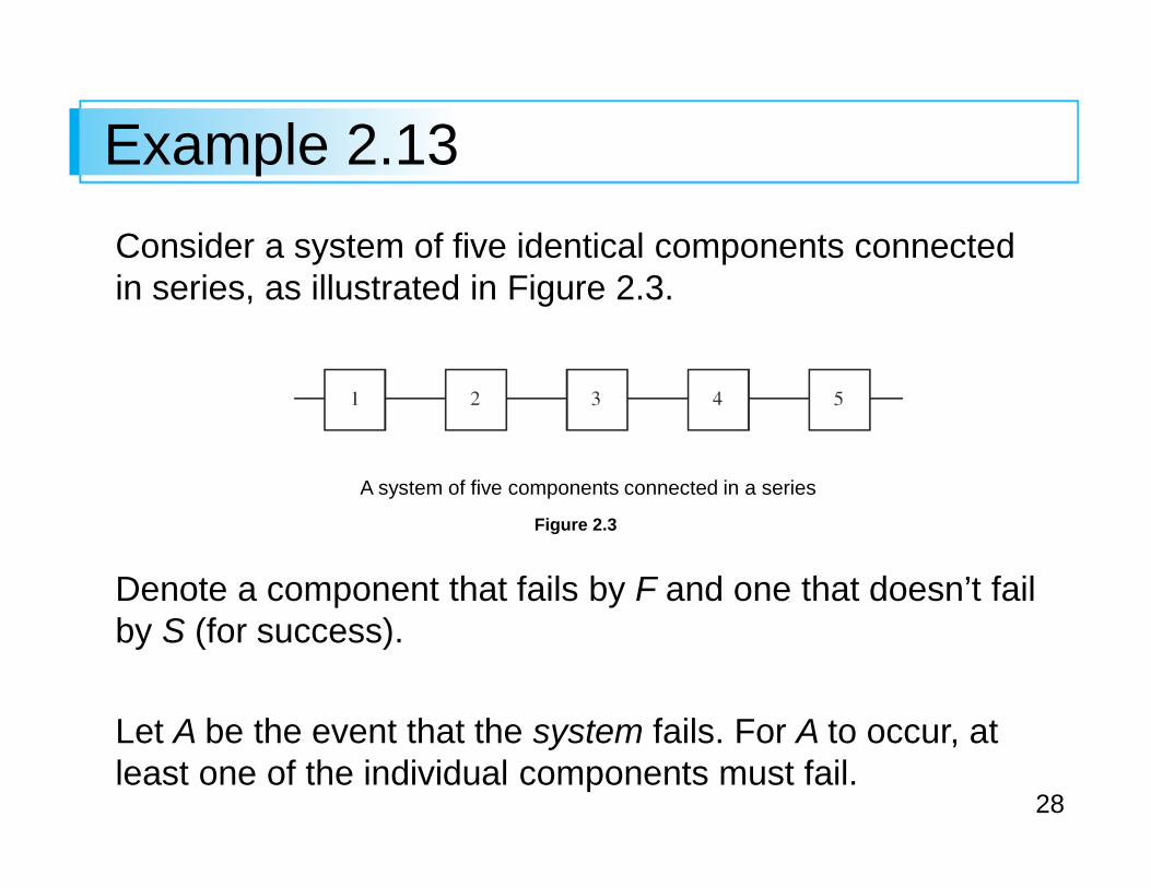
28
Example 2.13
Consider a system of five identical components connected in series, as illustrated in Figure 2.3.
Denote a component that fails by F and one that doesn’t fail by S (for success).
Let A be the event that the system fails. For A to occur, at least one of the individual components must fail.
Figure 2.3
A system of five components connected in a series
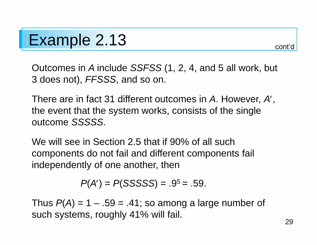
29
Example 2.13
Outcomes in A include SSFSS (1, 2, 4, and 5 all work, but 3 does not), FFSSS, and so on.
There are in fact 31 different outcomes in A. However, A′,the event that the system works, consists of the singleoutcome SSSSS.
We will see in Section 2.5 that if 90% of all such components do not fail and different components fail independently of one another, then
P(A′) = P(SSSSS) = .95 = .59.
Thus P(A) = 1 – .59 = .41; so among a large number of such systems, roughly 41% will fail.
cont’d
30
More Probability Properties
In general, the foregoing proposition is useful when the event of interest can be expressed as “at least . . . ,” since then the complement “less than . . .” may be easier to work with (in some problems, “more than . . .” is easier to deal with than “at most . . .”).
When you are having difficulty calculating P(A) directly, think of determining P(A′).
Proposition
31
More Probability Properties
This is because 1 = P(A) + P(A′) ≥ P(A) since P(A′) ≥ 0.
When events A and B are mutually exclusive,P(A ∪ B) = P(A) + P(B).
For events that are not mutually exclusive, adding P(A) and P(B) results in “doublecounting” outcomes in the intersection. The next result shows how to correct for this.
Proposition
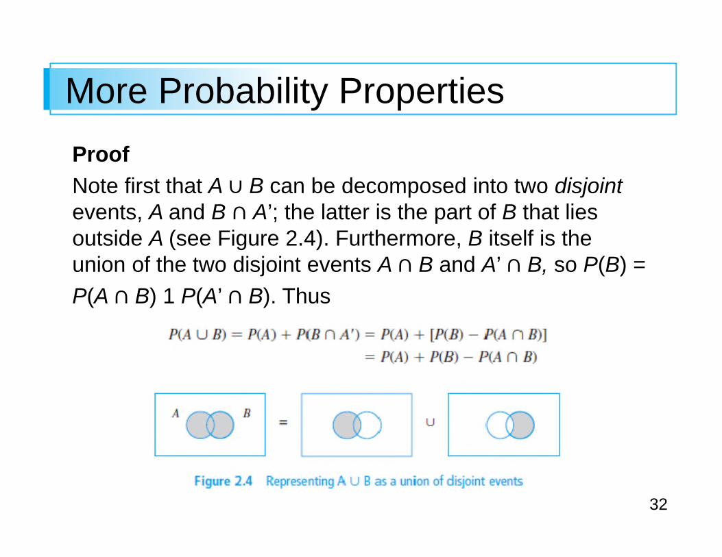
32
More Probability Properties
Proof
Note first that A B can be decomposed into two disjoint events, A and B A’; the latter is the part of B that lies outside A (see Figure 2.4). Furthermore, B itself is the union of the two disjoint events A B and A’ B, so P(B) =
P(A B) 1 P(A’ B). Thus
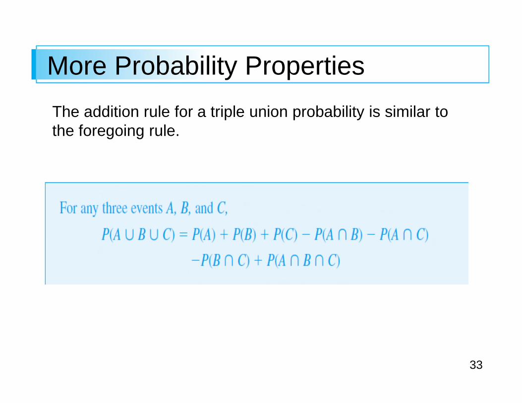
33
More Probability Properties
The addition rule for a triple union probability is similar to the foregoing rule.
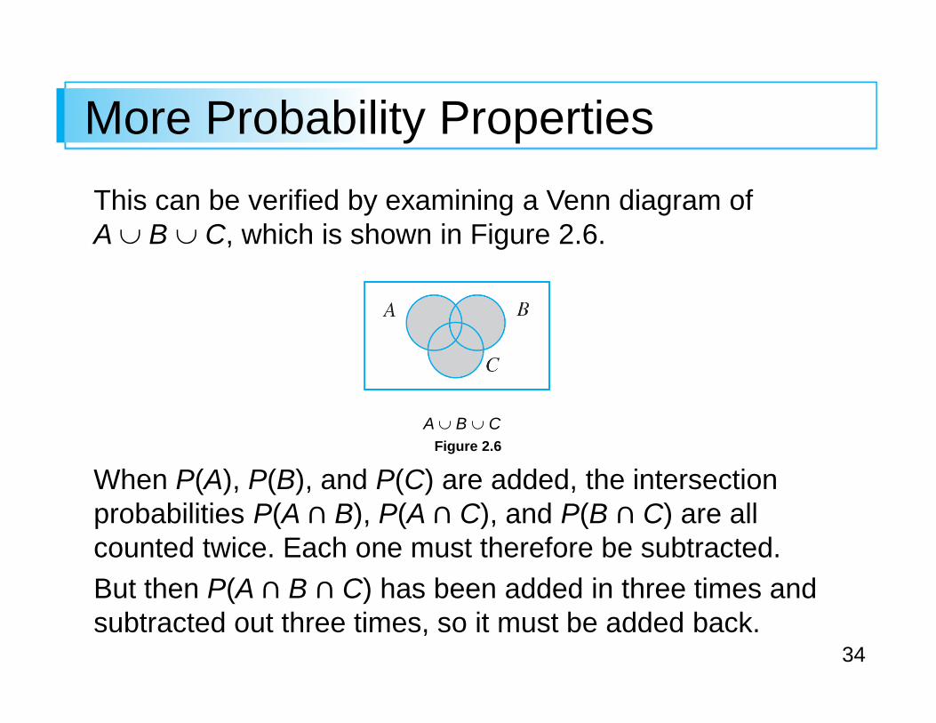
34
More Probability Properties
This can be verified by examining a Venn diagram ofA ∪ B ∪ C, which is shown in Figure 2.6.
When P(A), P(B), and P(C) are added, the intersection probabilities P(A B), P(A C), and P(B C) are all counted twice. Each one must therefore be subtracted.
But then P(A B C) has been added in three times and subtracted out three times, so it must be added back.
Figure 2.6
A ∪ B ∪ C
35
More Probability Properties
In general, the probability of a union of k events is obtained
by summing individual event probabilities, subtracting double intersection probabilities, adding triple intersection probabilities, subtracting quadruple intersection robabilities,
and so on.
36
Determining Probabilities Systematically
37
Determining Probabilities Systematically
Consider a sample space that is either finite or “countably infinite” (the latter means that outcomes can be listed in an infinite sequence, so there is a first outcome, a secondoutcome, a third outcome, and so on—for example, the battery testing scenario of Example 12).
Let E1, E2, E3, … denote the corresponding simple events, each consisting of a single outcome.
38
Determining Probabilities Systematically
A sensible strategy for probability computation is to first determine each simple event probability, with the requirement that ΣP(Ei) = 1.
Then the probability of any compound event A is computed by adding together the P(Ei)’s for all Ei’s in A:
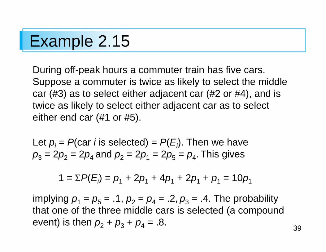
39
Example 2.15
During off-peak hours a commuter train has five cars. Suppose a commuter is twice as likely to select the middle car (#3) as to select either adjacent car (#2 or #4), and is twice as likely to select either adjacent car as to select either end car (#1 or #5).
Let pi = P(car i is selected) = P(Ei). Then we havep3 = 2p2 = 2p4 and p2 = 2p1 = 2p5 = p4. This gives
1 = ΣP(Ei) = p1 + 2p1 + 4p1 + 2p1 + p1 = 10p1
implying p1 = p5 = .1, p2 = p4 = .2, p3 = .4. The probability that one of the three middle cars is selected (a compound event) is then p2 + p3 + p4 = .8.

40
Equally Likely Outcomes

41
Equally Likely Outcomes
In many experiments consisting of N outcomes, it is reasonable to assign equal probabilities to all N simple events.
These include such obvious examples as tossing a fair coin or fair die once or twice (or any fixed number of times), or selecting one or several cards from a well-shuffled deck of 52. With p = P(Ei) for every i,
That is, if there are N equally likely outcomes, the probability for each is
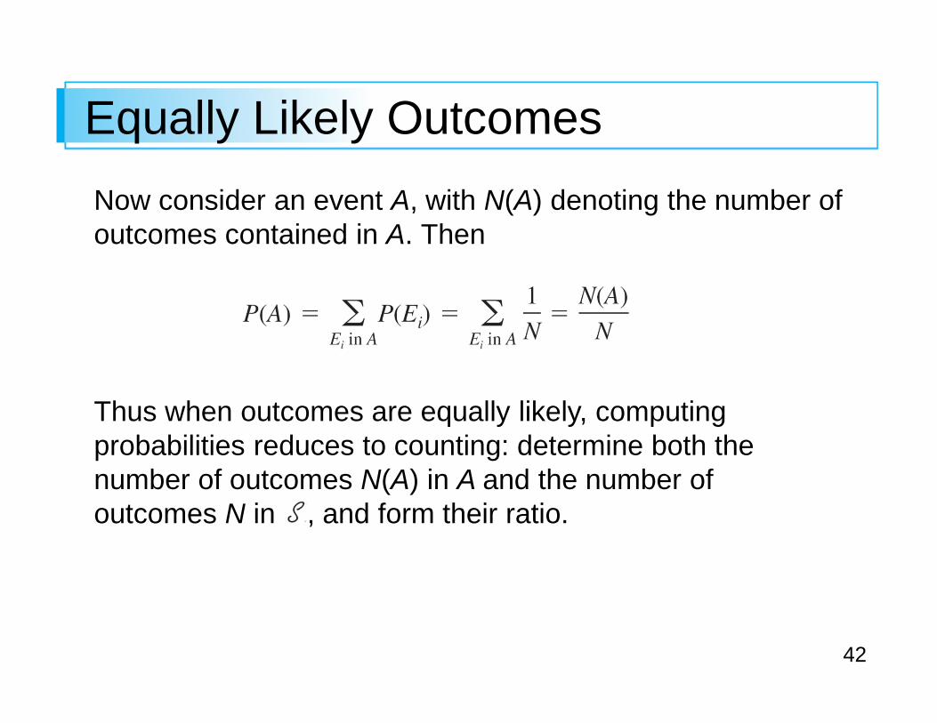
42
Equally Likely Outcomes
Now consider an event A, with N(A) denoting the number of outcomes contained in A. Then
Thus when outcomes are equally likely, computing probabilities reduces to counting: determine both the number of outcomes N(A) in A and the number of outcomes N in , and form their ratio.
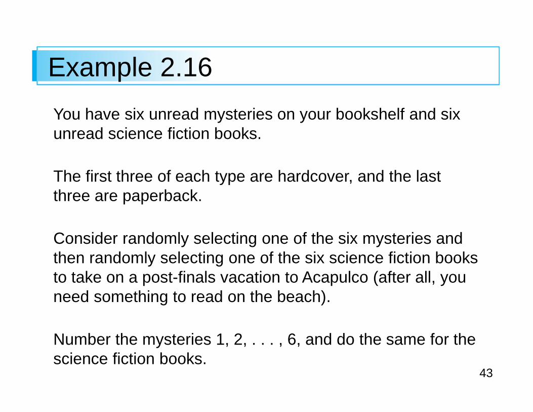
43
Example 2.16
You have six unread mysteries on your bookshelf and six unread science fiction books.
The first three of each type are hardcover, and the last three are paperback.
Consider randomly selecting one of the six mysteries and then randomly selecting one of the six science fiction books to take on a post-finals vacation to Acapulco (after all, you need something to read on the beach).
Number the mysteries 1, 2, . . . , 6, and do the same for the science fiction books.
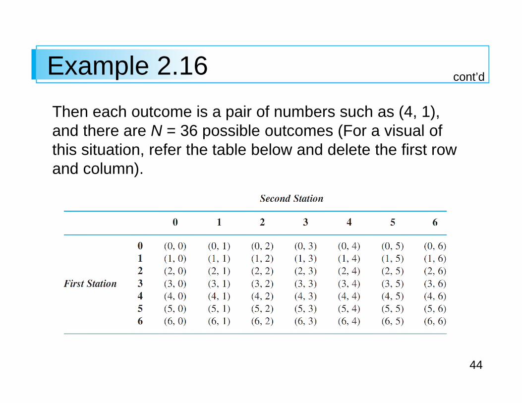
44
Example 2.16
Then each outcome is a pair of numbers such as (4, 1), and there are N = 36 possible outcomes (For a visual of this situation, refer the table below and delete the first row and column).
cont’d
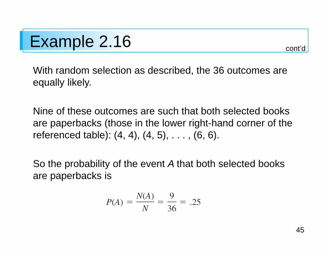
45
Example 2.16
With random selection as described, the 36 outcomes are equally likely.
Nine of these outcomes are such that both selected books are paperbacks (those in the lower right-hand corner of the referenced table): (4, 4), (4, 5), . . . , (6, 6).
So the probability of the event A that both selected books are paperbacks is
cont’d

Copyright © Cengage Learning. All rights reserved.
Probability
Copyright © Cengage Learning. All rights reserved.
2.3 Counting Techniques
3
Counting Techniques
When the various outcomes of an experiment are equally likely (the same probability is assigned to each simple event), the task of computing probabilities reduces to counting.
Letting N denote the number of outcomes in a sample space and N(A) represent the number of outcomes contained in an event A,
(2.1)
4
Counting Techniques
If a list of the outcomes is easily obtained and N is small, then N and N(A) can be determined without the benefit of any general counting principles.
There are, however, many experiments for which the effort involved in constructing such a list is prohibitive because N is quite large.
By exploiting some general counting rules, it is possible to compute probabilities of the form (2.1) without a listing of outcomes.
These rules are also useful in many problems involving outcomes that are not equally likely.

5
The Product Rule for Ordered Pairs
6
The Product Rule for Ordered Pairs
Our first counting rule applies to any situation in which a set (event) consists of ordered pairs of objects and we wish to count the number of such pairs.
By an ordered pair, we mean that, if O1 and O2 are objects, then the pair (O1, O2) is different from the pair (O2, O1).
For example, if an individual selects one airline for a trip from Los Angeles to Chicago and (after transacting business in Chicago) a second one for continuing on to New York, one possibility is (American, United), another is (United, American), and still another is (United, United).
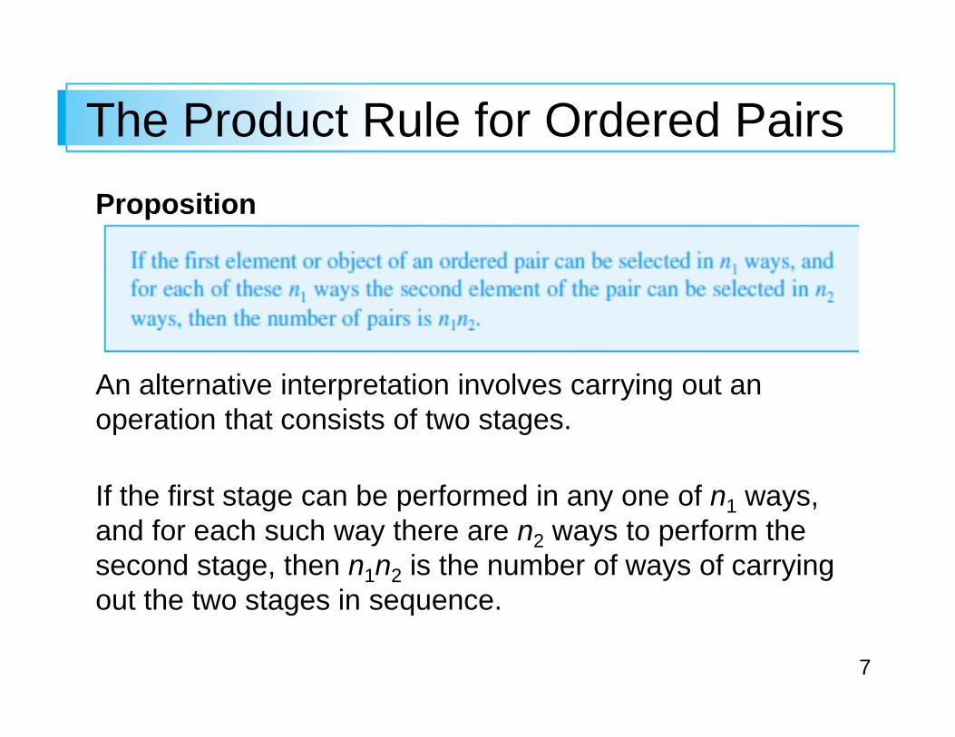
7
The Product Rule for Ordered Pairs
Proposition
An alternative interpretation involves carrying out an operation that consists of two stages.
If the first stage can be performed in any one of n1 ways, and for each such way there are n2 ways to perform the second stage, then n1n2 is the number of ways of carrying out the two stages in sequence.
8
Example 2.18
A family has just moved to a new city and requires the services of both an obstetrician and a pediatrician. There are two easily accessible medical clinics, each having two obstetricians and three pediatricians.
The family will obtain maximum health insurance benefits by joining a clinic and selecting both doctors from that clinic. In how many ways can this be done?
Denote the obstetricians by O1, O2, O3, and O4 and the pediatricians by P1, . . . ., P6.
9
Example 2.18
Then we wish the number of pairs (Oi, Pj) for which Oi and Pj are associated with the same clinic.
Because there are four obstetricians, n1 = 4, and for each there are three choices of pediatrician, so n2 = 3.
Applying the product rule gives N = n1n2 = 12 possible choices.
cont’d
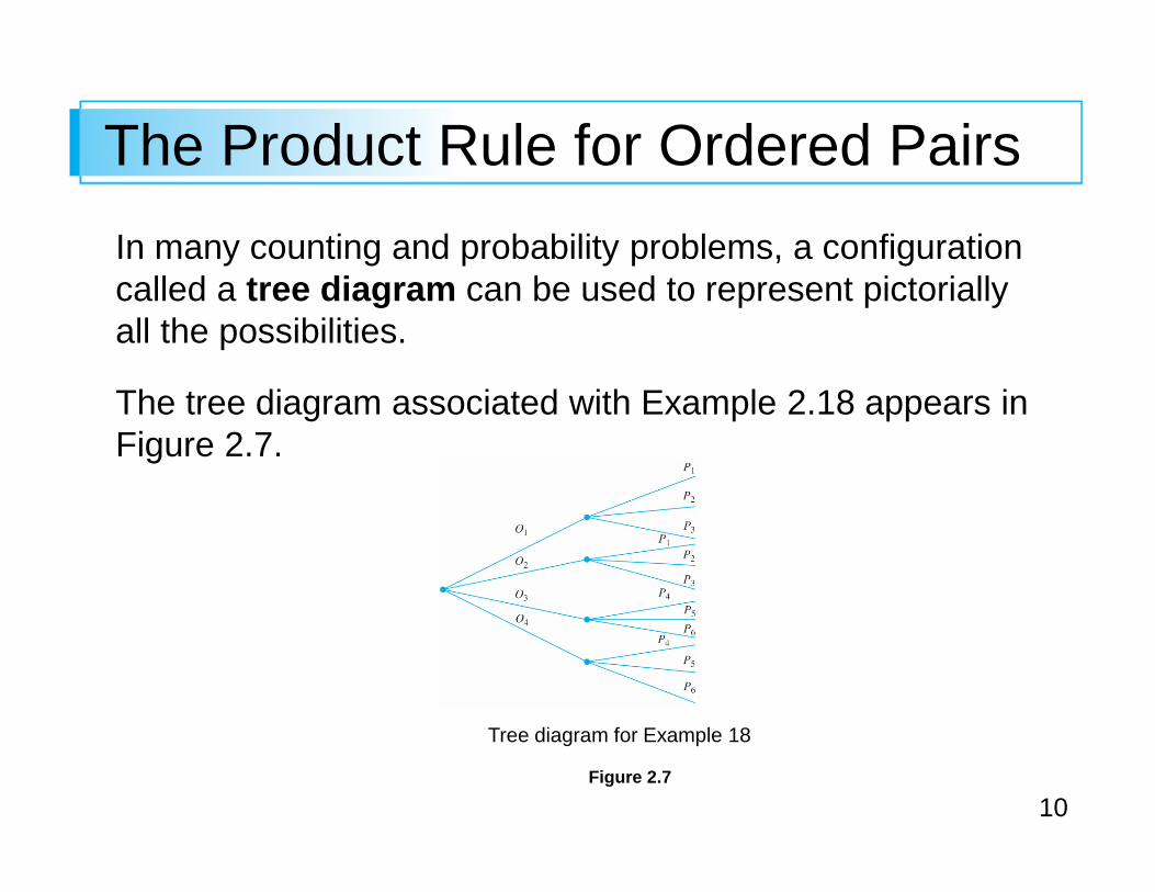
10
The Product Rule for Ordered Pairs
In many counting and probability problems, a configuration called a tree diagram can be used to represent pictorially all the possibilities.
The tree diagram associated with Example 2.18 appears in Figure 2.7.
Figure 2.7
Tree diagram for Example 18
11
The Product Rule for Ordered Pairs
Starting from a point on the left side of the diagram, for each possible first element of a pair a straight-line segment emanates rightward.
Each of these lines is referred to as a first-generation branch.
Now for any given first-generation branch we construct another line segment emanating from the tip of the branch for each possible choice of a second element of the pair.
12
The Product Rule for Ordered Pairs
Each such line segment is a second-generation branch. Because there are four obstetricians, there are four first-generation branches, and three pediatricians for each obstetrician yields three second-generation branches emanating from each first-generation branch.
Generalizing, suppose there are n1 first-generation branches, and for each first generation branch there are n2 second-generation branches.
The total number of second-generation branches is then n1n2.
13
The Product Rule for Ordered Pairs
Since the end of each second-generation branch corresponds to exactly one possible pair (choosing a first element and then a second puts us at the end of exactly one second-generation branch), there are n1n2 pairs, verifying the product rule.
The construction of a tree diagram does not depend on having the same number of second-generation branches emanating from each first-generation branch.
14
The Product Rule for Ordered Pairs
If the second clinic had four pediatricians, then there would be only three branches emanating from two of the first-generation branches and four emanating from each of the other two first-generation branches.
A tree diagram can thus be used to represent pictorially experiments other than those to which the product rule applies.

15
A More General Product Rule
16
A More General Product Rule
If a six-sided die is tossed five times in succession rather than just twice, then each possible outcome is an ordered collection of five numbers such as (1, 3, 1, 2, 4) or (6, 5, 2, 2, 2).
We will call an ordered collection of k objects a k-tuple (so a pair is a 2-tuple and a triple is a 3-tuple).
Each outcome of the die-tossing experiment is then a 5-tuple.
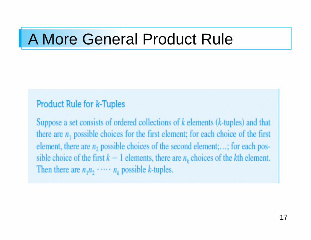
17
A More General Product Rule
18
A More General Product Rule
An alternative interpretation involves carrying out an operation in k stages.
If the first stage can be performed in any one of n1 ways, and for each such way there are n2 ways to perform the second stage, and for each way of performing the first two stages there are n3 ways to perform the 3rd stage, and so on, then n1n2 · · · nk is the number of ways to carry out the entire k-stage operation in sequence.
This more general rule can also be visualized with a tree diagram. For the case k = 3, simply add an appropriate number of 3rd generation branches to the tip of each 2nd generation branch.
19
A More General Product Rule
If, for example, a college town has four pizza places, a theater complex with six screens, and three places to go dancing, then there would be four 1st generation branches, six 2nd generation branches emanating from the tip of each 1st generation branch, and three 3rd generation branches leading off each 2nd generation branch.
Each possible 3-tuple corresponds to the tip of a 3rd generation branch.
20
Example 2.19
Example 17 continued…
Suppose the home remodeling job involves first purchasing several kitchen appliances. They will all be purchased from the same dealer, and there are five dealers in the area.
With the dealers denoted by D1, . . . , D5, there areN = n1n2n3 = (5)(12)(9) = 540 3-tuples of the form (Di, Pj, Qk), so there are 540 ways to choose first an appliance dealer, then a plumbing contractor, and finally an electrical contractor.

21
Permutations and Combinations
22
Permutations and Combinations
Consider a group of n distinct individuals or objects (“distinct” means that there is some characteristic that differentiates any particular individual or object from any other).
How many ways are there to select a subset of size k from the group?
For example, if a Little League team has 15 players on its roster, how many ways are there to select 9 players to form a starting lineup?
23
Permutations and Combinations
Or if a university bookstore sells ten different laptop computers but has room to display only three of them, in how many ways can the three be chosen?
An answer to the general question just posed requires that we distinguish between two cases. In some situations, such as the baseball scenario, the order of selection is important.
For example, Angela being the pitcher and Ben the catcher gives a different lineup from the one in which Angela is catcher and Ben is pitcher.
24
Permutations and Combinations
Often, though, order is not important and one is interested only in which individuals or objects are selected, as would be the case in the laptop display scenario.
Definition
25
Permutations and Combinations
The number of permutations can be determined by using our earlier counting rule for k-tuples. Suppose, for example, that a college of engineering has seven departments, which we denote by a, b, c, d, e, f, and g.
Each department has one representative on the college’s student council. From these seven representatives, one is to be chosen chair, another is to be selected vice-chair, and a third will be secretary.
How many ways are there to select the three officers? That is, how many permutations of size 3 can be formed from the 7 representatives?
26
Permutations and Combinations
To answer this question, think of forming a triple (3-tuple) in which the first element is the chair, the second is the vice-chair, and the third is the secretary.
One such triple is (a, g, b), another is (b, g, a), and yet another is (d, f, b). Now the chair can be selected in any ofn1 = 7 ways.
For each way of selecting the chair, there are n2 = 6 ways to select the vice-chair, and hence 7 × 6 = 42 (chair, vice-chair) pairs.
27
Permutations and Combinations
Finally, for each way of selecting a chair and vice-chair, there are n3 = 5 ways of choosing the secretary. This gives
P3,7 = (7)(6)(5) = 210
as the number of permutations of size 3 that can be formed from 7 distinct individuals. A tree diagram representation would show three generations of branches.
The expression for P3,7 can be rewritten with the aid of factorial notation. Recall that 7! (read “7 factorial”) is compact notation for the descending product of integers (7)(6)(5)(4)(3)(2)(1).
28
Permutations and Combinations
More generally, for any positive integer m,
m! = m(m – 1)(m – 2) · · · · (2)(1.) This gives 1! = 1, and we also define 0! = 1. Then
P3,7 = (7)(6)(5) =
More generally,
Pk,n = n(n – 1)(n – 2) · · · · (n – (k – 2))(n – (k – 1))
Multiplying and dividing this by (n – k)! gives a compact expression for the number of permutations.
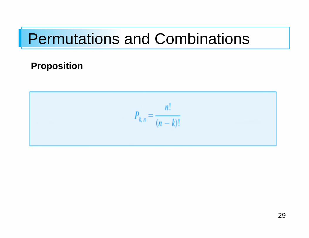
29
Permutations and Combinations
Proposition
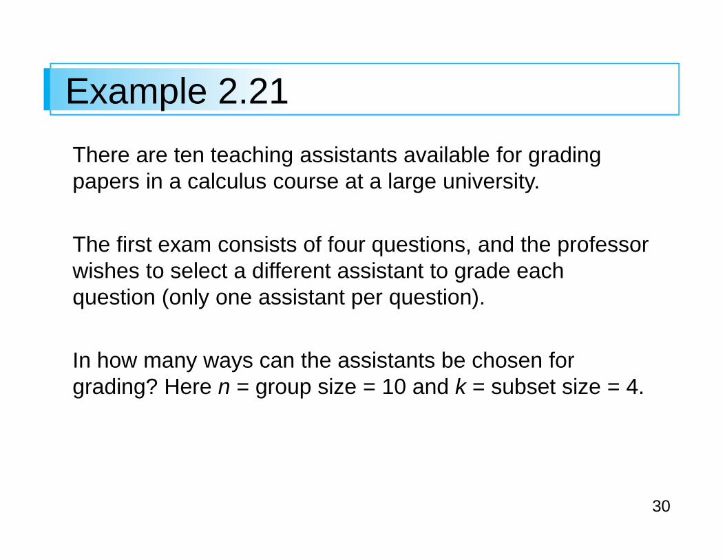
30
Example 2.21
There are ten teaching assistants available for grading papers in a calculus course at a large university.
The first exam consists of four questions, and the professor wishes to select a different assistant to grade each question (only one assistant per question).
In how many ways can the assistants be chosen for grading? Here n = group size = 10 and k = subset size = 4.
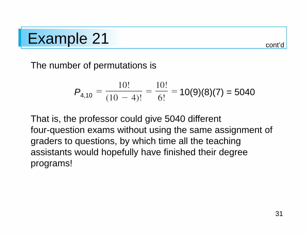
31
Example 21
The number of permutations is
P4,10 10(9)(8)(7) = 5040
That is, the professor could give 5040 different four-question exams without using the same assignment of graders to questions, by which time all the teaching assistants would hopefully have finished their degree programs!
cont’d
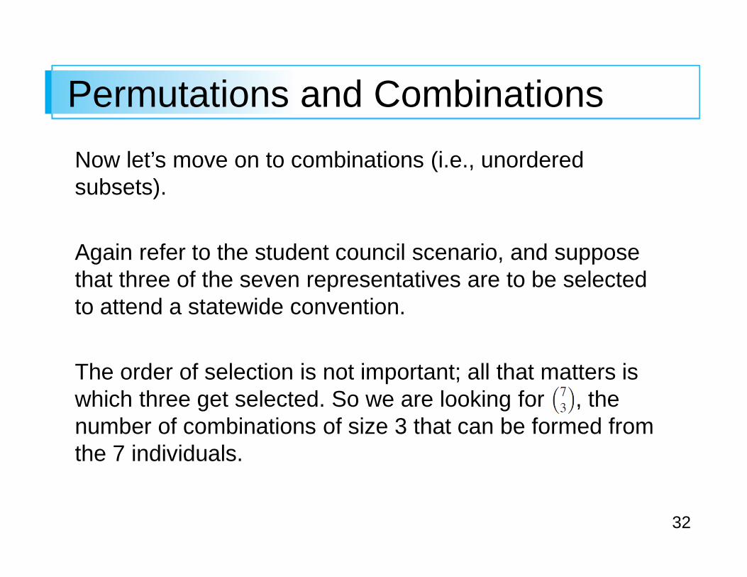
32
Permutations and Combinations
Now let’s move on to combinations (i.e., unordered subsets).
Again refer to the student council scenario, and suppose that three of the seven representatives are to be selected to attend a statewide convention.
The order of selection is not important; all that matters is which three get selected. So we are looking for , the number of combinations of size 3 that can be formed from the 7 individuals.
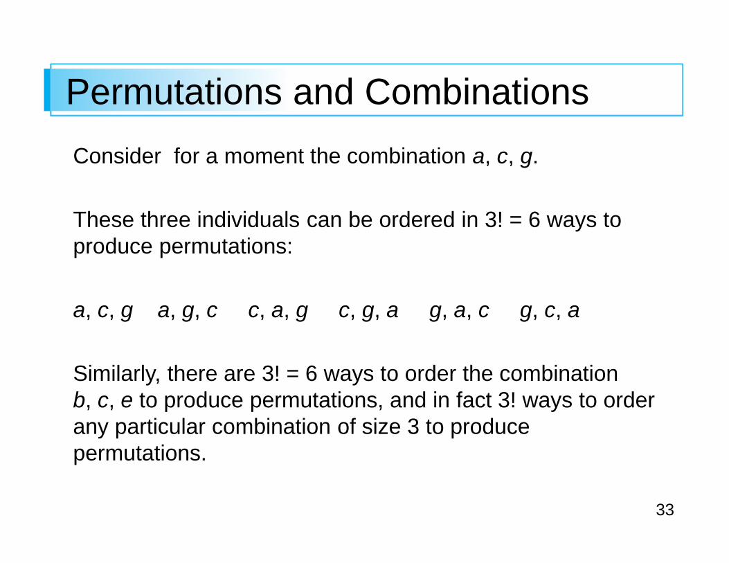
33
Permutations and Combinations
Consider for a moment the combination a, c, g.
These three individuals can be ordered in 3! = 6 ways to produce permutations:
a, c, g a, g, c c, a, g c, g, a g, a, c g, c, a
Similarly, there are 3! = 6 ways to order the combination b, c, e to produce permutations, and in fact 3! ways to order any particular combination of size 3 to produce permutations.
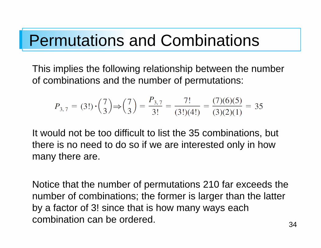
34
Permutations and Combinations
This implies the following relationship between the number of combinations and the number of permutations:
It would not be too difficult to list the 35 combinations, but there is no need to do so if we are interested only in how many there are.
Notice that the number of permutations 210 far exceeds the number of combinations; the former is larger than the latter by a factor of 3! since that is how many ways each combination can be ordered.
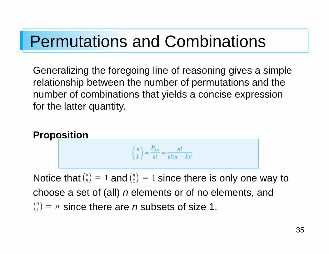
35
Permutations and Combinations
Generalizing the foregoing line of reasoning gives a simple relationship between the number of permutations and the number of combinations that yields a concise expression for the latter quantity.
Proposition
Notice that and since there is only one way to
choose a set of (all) n elements or of no elements, and
since there are n subsets of size 1.
36
Example 2.22
A particular iPod playlist contains 100 songs, 10 of which are by the Beatles.
Suppose the shuffle feature is used to play the songs in random order (the randomness of the shuffling process is investigated in “Does Your iPod Really Play Favorites?”
What is the probability that the first Beatles song heard is the fifth song played?
In order for this event to occur, it must be the case that the first four songs played are not Beatles’ songs (NBs) and that the fifth song is by the Beatles (B).
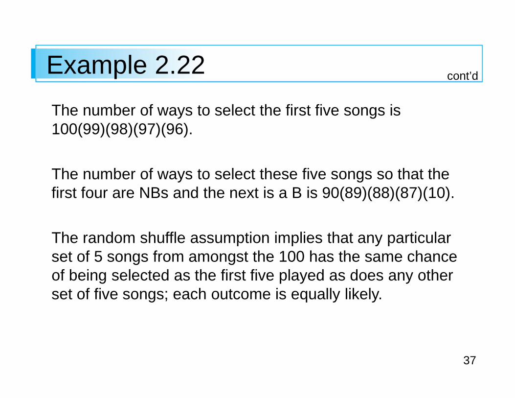
37
Example 2.22
The number of ways to select the first five songs is 100(99)(98)(97)(96).
The number of ways to select these five songs so that the first four are NBs and the next is a B is 90(89)(88)(87)(10).
The random shuffle assumption implies that any particular set of 5 songs from amongst the 100 has the same chance of being selected as the first five played as does any other set of five songs; each outcome is equally likely.
cont’d
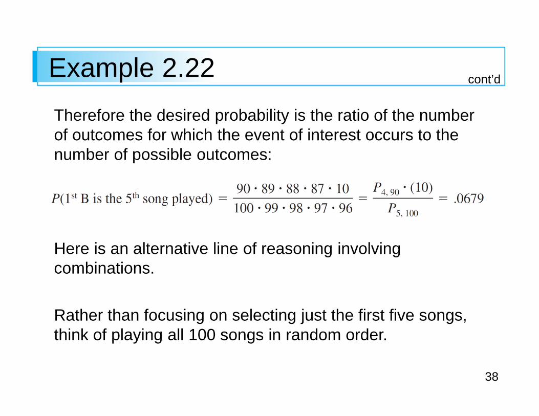
38
Example 2.22
Therefore the desired probability is the ratio of the number of outcomes for which the event of interest occurs to the number of possible outcomes:
Here is an alternative line of reasoning involving combinations.
Rather than focusing on selecting just the first five songs, think of playing all 100 songs in random order.
cont’d
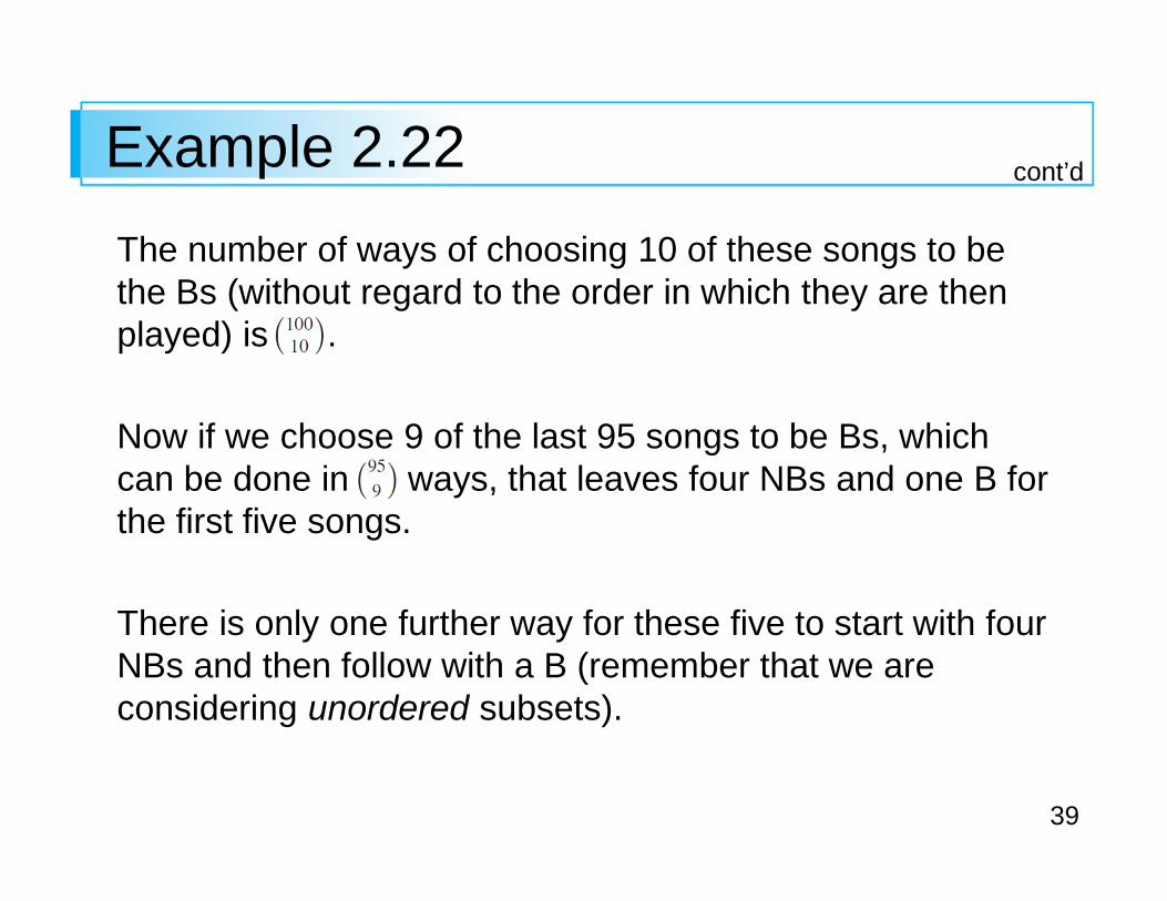
39
Example 2.22
The number of ways of choosing 10 of these songs to be the Bs (without regard to the order in which they are then played) is .
Now if we choose 9 of the last 95 songs to be Bs, which can be done in ways, that leaves four NBs and one B for the first five songs.
There is only one further way for these five to start with four NBs and then follow with a B (remember that we are considering unordered subsets).
cont’d
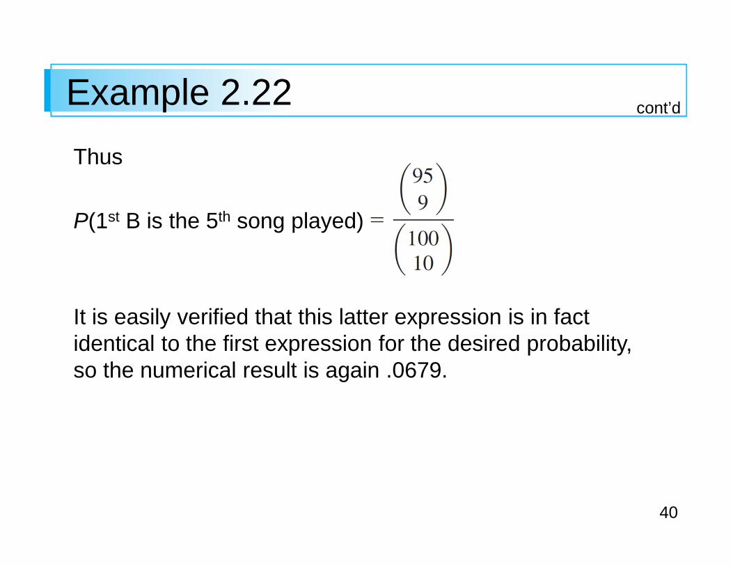
40
Example 2.22
Thus
P(1st B is the 5th song played)
It is easily verified that this latter expression is in fact identical to the first expression for the desired probability, so the numerical result is again .0679.
cont’d
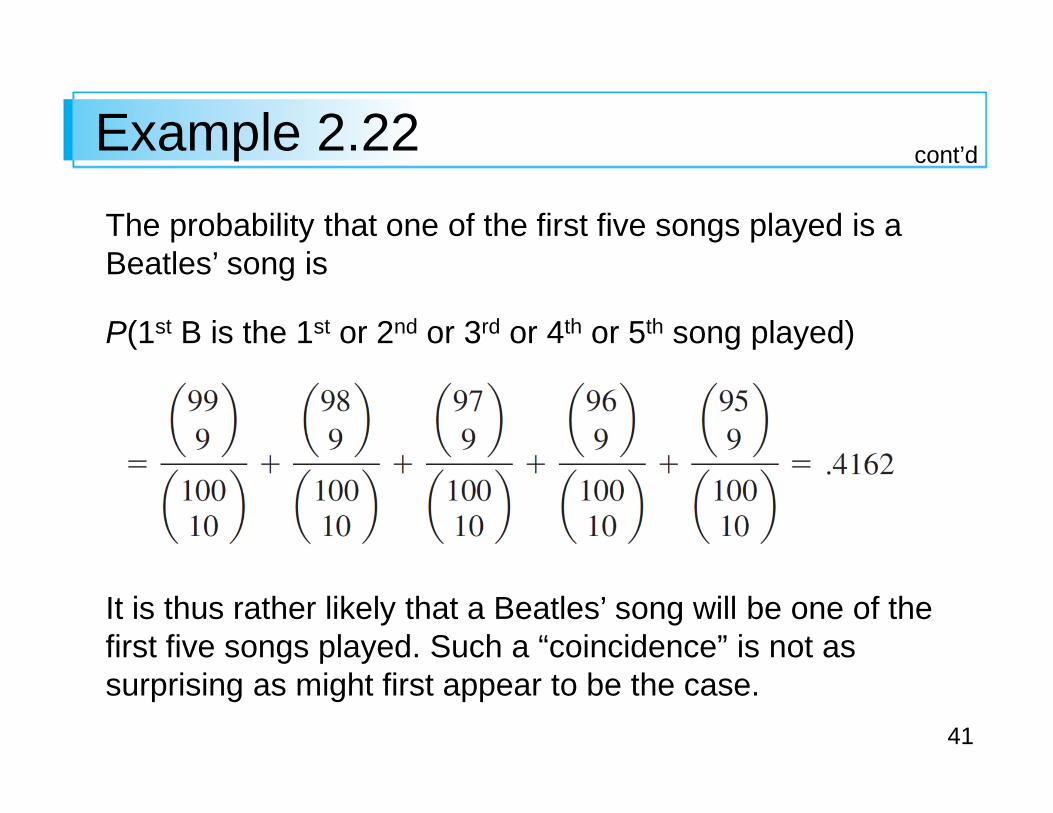
41
Example 2.22
The probability that one of the first five songs played is a Beatles’ song is
P(1st B is the 1st or 2nd or 3rd or 4th or 5th song played)
It is thus rather likely that a Beatles’ song will be one of the first five songs played. Such a “coincidence” is not as surprising as might first appear to be the case.
cont’d
Copyright © Cengage Learning. All rights reserved.
Probability
Copyright © Cengage Learning. All rights reserved.
2.4 Conditional Probability
3
Conditional Probability
The probabilities assigned to various events depend on what is known about the experimental situation when the assignment is made.
Subsequent to the initial assignment, partial information relevant to the outcome of the experiment may become available. Such information may cause us to revise some of our probability assignments.
For a particular event A, we have used P(A) to represent the probability, assigned to A; we now think of P(A) as the original, or unconditional probability, of the event A.
4
Conditional Probability
In this section, we examine how the information “an event B has occurred” affects the probability assigned to A.
For example, A might refer to an individual having a particular disease in the presence of certain symptoms.
If a blood test is performed on the individual and the result is negative (B = negative blood test), then the probability of having the disease will change (it should decrease, but not usually to zero, since blood tests are not infallible).
5
Conditional Probability
We will use the notation P(A | B) to represent the conditional probability of A given that the event B has occurred. B is the “conditioning event.”
As an example, consider the event A that a randomly selected student at your university obtained all desired classes during the previous term’s registration cycle. Presumably P(A) is not very large.
However, suppose the selected student is an athlete who gets special registration priority (the event B). Then P(A | B) should be substantially larger than P(A), although perhaps still not close to 1.
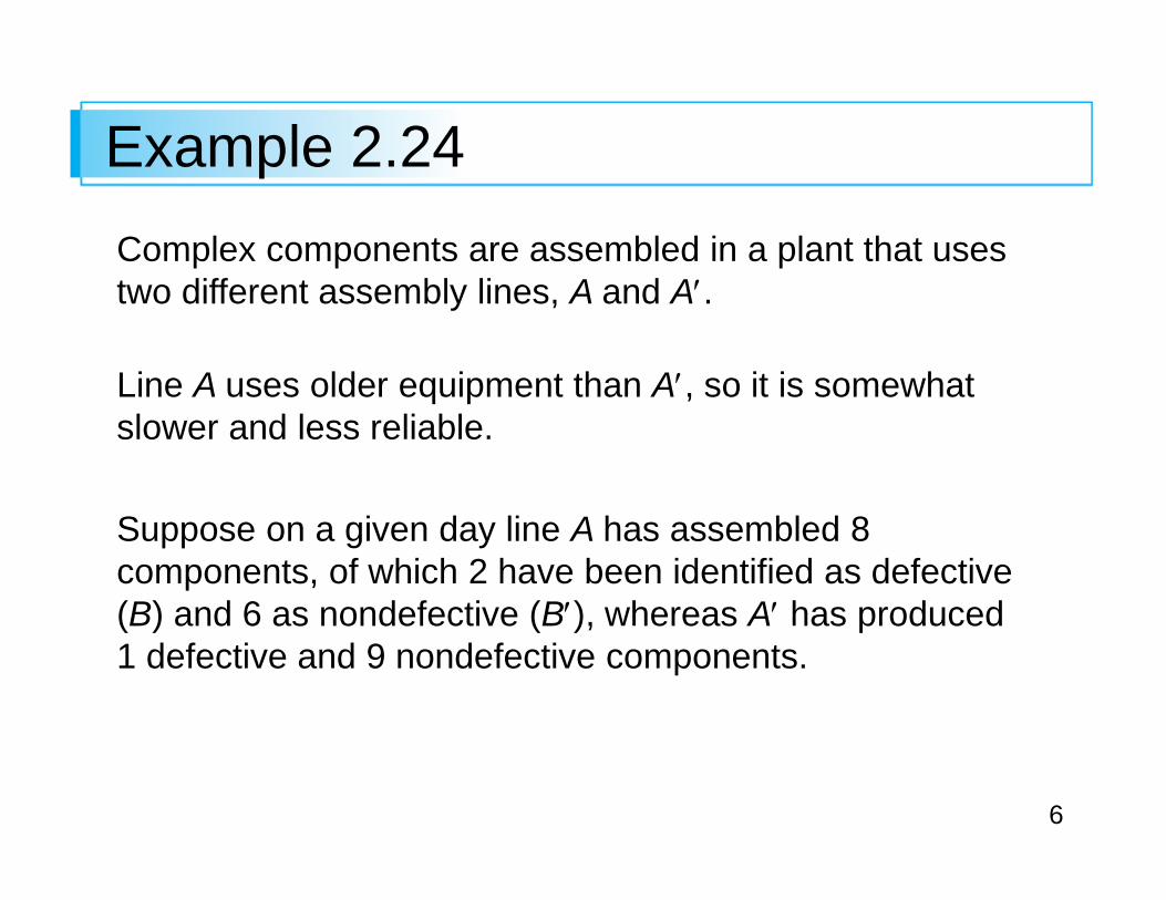
6
Example 2.24
Complex components are assembled in a plant that uses two different assembly lines, A and A′.
Line A uses older equipment than A′, so it is somewhat slower and less reliable.
Suppose on a given day line A has assembled 8 components, of which 2 have been identified as defective (B) and 6 as nondefective (B′), whereas A′ has produced 1 defective and 9 nondefective components.
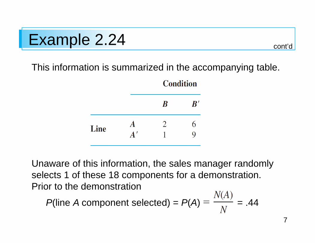
7
Example 2.24
This information is summarized in the accompanying table.
Unaware of this information, the sales manager randomly selects 1 of these 18 components for a demonstration.Prior to the demonstration
P(line A component selected) = P(A) = .44
cont’d
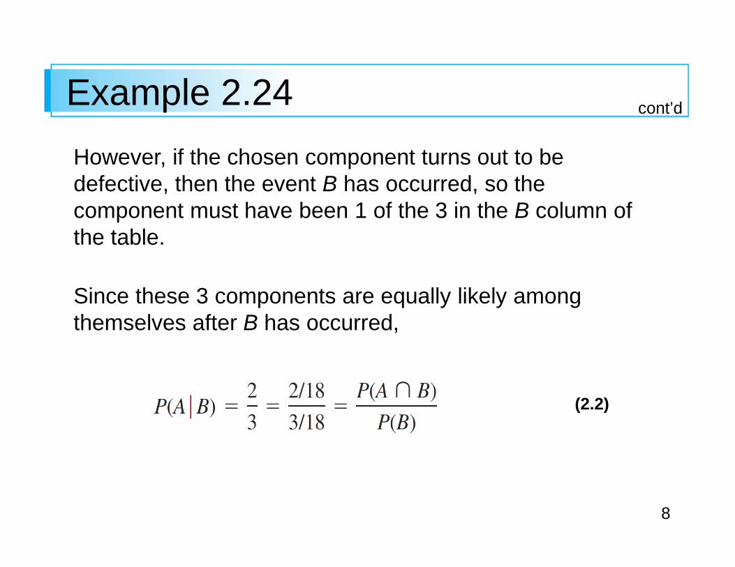
8
Example 2.24
However, if the chosen component turns out to be defective, then the event B has occurred, so the component must have been 1 of the 3 in the B column of the table.
Since these 3 components are equally likely amongthemselves after B has occurred,
(2.2)
cont’d
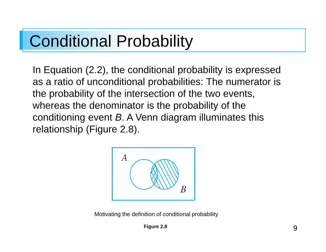
9
Conditional Probability
In Equation (2.2), the conditional probability is expressed as a ratio of unconditional probabilities: The numerator is the probability of the intersection of the two events, whereas the denominator is the probability of the conditioning event B. A Venn diagram illuminates this relationship (Figure 2.8).
Motivating the definition of conditional probability
Figure 2.8
10
Conditional Probability
Given that B has occurred, the relevant sample space is no longer S but consists of outcomes in B; A has occurred if and only if one of the outcomes in the intersection occurred, so the conditional probability of A given B is
proportional to
The proportionality constant 1/P(B) is used to ensure that the probability P(B | B) of the new sample space B equals 1.
11
The Definition of Conditional Probability
12
The Definition of Conditional Probability
Example 2.24 demonstrates that when outcomes are equally likely, computation of conditional probabilities can be based on intuition.
When experiments are more complicated, though, intuition may fail us, so a general definition of conditional probability is needed that will yield intuitive answers in simple problems.
The Venn diagram and Equation (2.2) suggest how to proceed.
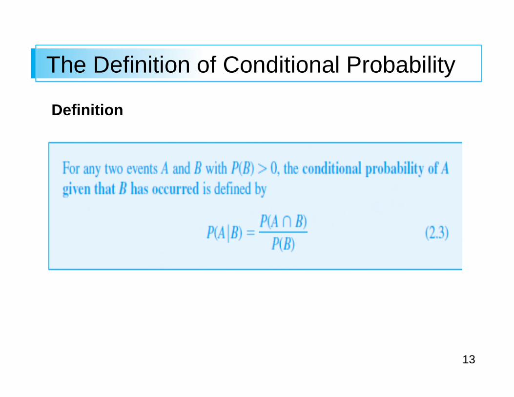
13
The Definition of Conditional Probability
Definition
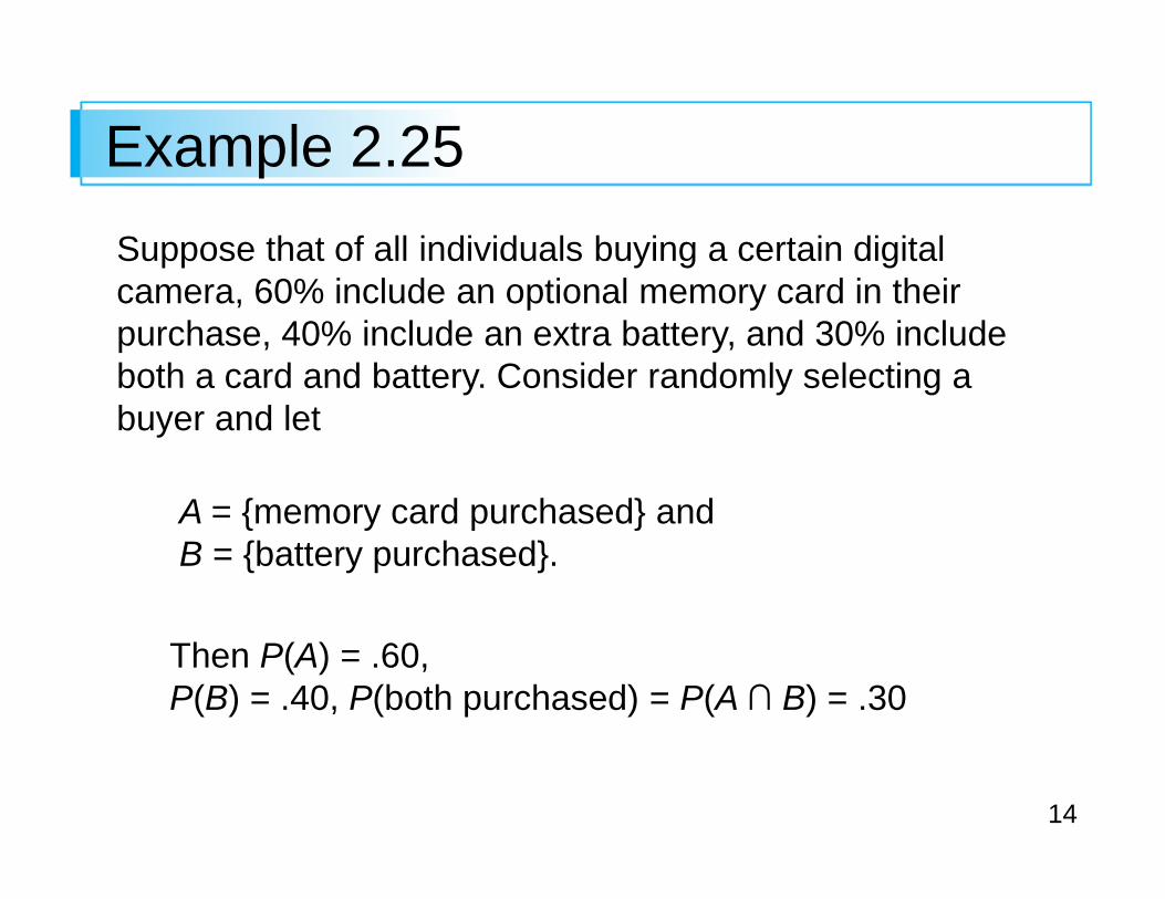
14
Example 2.25
Suppose that of all individuals buying a certain digital camera, 60% include an optional memory card in their purchase, 40% include an extra battery, and 30% include both a card and battery. Consider randomly selecting a buyer and let
A = {memory card purchased} andB = {battery purchased}.
Then P(A) = .60, P(B) = .40, P(both purchased) = P(A ∩ B) = .30
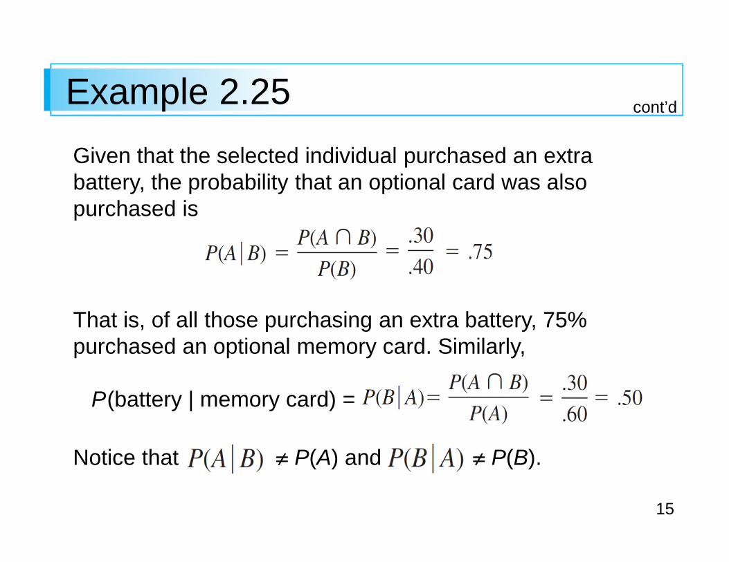
15
Example 2.25
Given that the selected individual purchased an extra battery, the probability that an optional card was also purchased is
That is, of all those purchasing an extra battery, 75% purchased an optional memory card. Similarly,
P(battery | memory card) =
Notice that ≠ P(A) and ≠ P(B).
cont’d
16
The Multiplication Rule for P(A ∩ B)
17
The Multiplication Rule for P(A ∩ B)
The definition of conditional probability yields the following result, obtained by multiplying both sides of Equation (2.3) by P(B).
The Multiplication Rule
This rule is important because it is often the case that P(A ∩ B) is desired, whereas both P(B) and can be specified from the problem description.
Consideration of gives P(A ∩ B) = P(A)
18
Example 2.27
Four individuals have responded to a request by a blood bank for blood donations. None of them has donated before, so their blood types are unknown. Suppose only type O+ is desired and only one of the four actually has this type. If the potential donors are selected in random order for typing, what is the probability that at least three individuals must be typed to obtain the desired type?
Making the identification
B = {first type not O+} and
A = {second type not O+}, P(B) =
19
Example 2.27
Given that the first type is not O+, two of the three
individuals left are not O+, so
The multiplication rule now gives
P(at least three individuals are typed) = P(A ∩ B)
cont’d
20
Example 2.27
The multiplication rule is most useful when the experiment consists of several stages in succession.
The conditioning event B then describes the outcome of the first stage and A the outcome of the second, so that
—conditioning on what occurs first—will often be known.
The rule is easily extended to experiments involvingmore than two stages.
cont’d
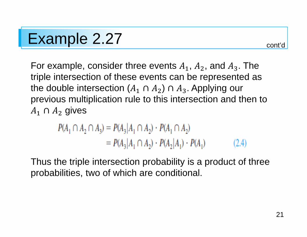
21
Example 2.27
For example, consider three events , , and . The triple intersection of these events can be represented as the double intersection ( ) . Applying our previous multiplication rule to this intersection and then to
gives
Thus the triple intersection probability is a product of three probabilities, two of which are conditional.
cont’d
22
Bayes’ Theorem
23
Bayes’ Theorem
The computation of a posterior probability from given prior probabilities P(Ai) and conditional probabilities
occupies a central position in elementary probability.
The general rule for such computations, which is really just a simple application of the multiplication rule, goes back to Reverend Thomas Bayes, who lived in the eighteenth century.
To state it we first need another result. Recall that events A1, . . . , Ak are mutually exclusive if no two have any common outcomes. The events are exhaustive if one Ai
must occur, so that A1 ∪ …∪ Ak =
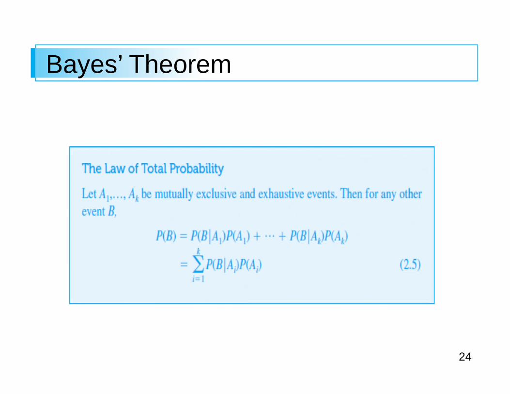
24
Bayes’ Theorem
25
Example 2.30
An individual has 3 different email accounts. Most of her messages, in fact 70%, come into account #1, whereas 20% come into account #2 and the remaining 10% into account #3.
Of the messages into account #1, only 1% are spam, whereas the corresponding percentages for accounts #2 and #3 are 2% and 5%, respectively.
What is the probability that a randomly selected message is spam?
26
Example 2.30
To answer this question, let’s first establish some notation:
Ai = {message is from account # i} for i = 1, 2, 3,
B = {message is spam}
Then the given percentages imply that
P(A1) = .70, P(A2) = .20, P(A3) = .10
cont’d
27
Example 2.30
Now it is simply a matter of substituting into the equation for the law of total probability:
P(B) = (.01)(.70) + (.02)(.20) + (.05)(.10) = .016
In the long run, 1.6% of this individual’s messages will be spam.
cont’d
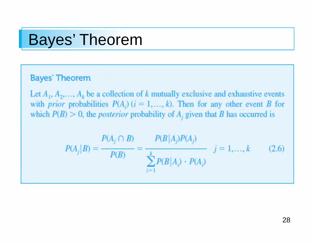
28
Bayes’ Theorem
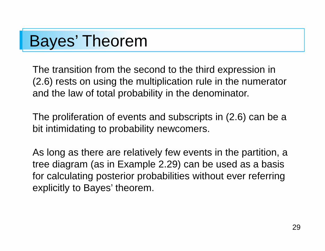
29
Bayes’ Theorem
The transition from the second to the third expression in (2.6) rests on using the multiplication rule in the numerator and the law of total probability in the denominator.
The proliferation of events and subscripts in (2.6) can be a bit intimidating to probability newcomers.
As long as there are relatively few events in the partition, a tree diagram (as in Example 2.29) can be used as a basis for calculating posterior probabilities without ever referring explicitly to Bayes’ theorem.