Deviation inequalities and moderate deviation principle ...reynaudb/jps/ergolim/BPSV_CIRM_2012.pdf · Université Blaise Pascal ... Figure: Cell division from E. J. Stewart and al

Introduction Goals Framework for the results Results Application

Deviation inequalities and moderatedeviation principle for Bifurcating Markov

Chains.

S. Valère BITSEKI PENDAjoint work with

(H. Djellout and A. Guillin)

Université Blaise PascalLaboratoire de Mathématiques

Colloque Jeunes Probabilistes Statisticiens, CIRM 2012


Outline

1 IntroductionMotivationThe model of bifurcating Markov chain

2 Goals

3 Framework for the results

4 Results

5 Application


Motivation

Guyon, J. Limit theorems for bifurcating markov chains.Application to the detection of cellular aging. Ann. Appl.Probab., (2007), Vol. 17, No. 5-6, pp. 1538-1569.

Escherichia Coli (E.Coli)

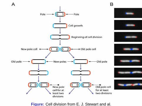
Figure: Cell division from E. J. Stewart and al.


Motivation

Guyon, J. Bize, A. Paul, G. Stewart, E.J. Delmas, J.F.Taddéi, F. Statistical study of cellular aging. CEMRACS2004 Proceedings, ESAIM Proceedings, (2005), 14, pp.100-114.


Motivation

First order bifurcating autoregressive process BAR(1)


Motivation


X

n


Motivation


L(X1) = ν, and ∀n ≥ 1,

X2n = α0Xn + β0 + ε2n

X2n+1 = α1Xn + β1 + ε2n+1,(1)


Motivation


where ν is a distribution probability on R, α0, α1 ∈ (−1, 1);β0, β1 ∈ R and

((ε2n, ε2n+1), n ≥ 1

)forms a sequence of

centered i.i.d bivariate random variables with covariancematrix

Γ = σ2(

1 ρρ 1

), σ2 > 0, ρ ∈ (−1, 1).


Motivation

θ = (α0, β0, α1, β1), σ and ρ.

H0 = (α0, β0) = (α1, β1) against H1 = (α0, β0) 6= (α1, β1).


Motivation

θ = (α0, β0, α1, β1), σ and ρ.H0 = (α0, β0) = (α1, β1) against H1 = (α0, β0) 6= (α1, β1).


Motivation

L(X1) = ν, and ∀n ≥ 1,

X2n = α0Xn + β0 + ε2n

X2n+1 = α1Xn + β1 + ε2n+1,(1)

where ν is a distribution probability on R, α0, α1 ∈ (−1, 1);β0, β1 ∈ R and

((ε2n, ε2n+1), n ≥ 1

)forms a sequence of

centered i.i.d bivariate random variables with covariance matrix

Γ = σ2(

1 ρρ 1

), σ2 > 0, ρ ∈ (−1, 1).

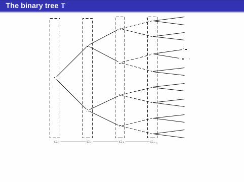
The binary tree T

G0 G1 G2 Grn

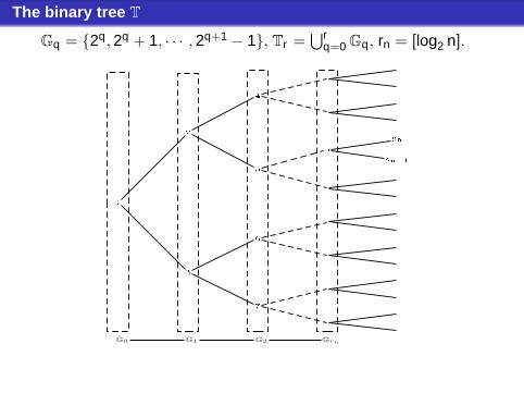
The binary tree T

Gq = 2q, 2q + 1, · · · , 2q+1 − 1, Tr =⋃r

q=0 Gq, rn = [log2 n].

G0 G1 G2 Grn


The model of bifurcating Markov chain

• (S,S)

• P : S × S2 → [0, 1] such that

P(., A) is measurable for all A ∈ S2,P(x , .) is a probability measure on (S2,S2) for all x ∈ S.

• P0(·, ·) = P(·, · ×S), P1(·, ·) = P(·, S× ·) and Q =P0 + P1

2.

• For all f ∈ B(S3),

Pf : x 7→ Pf (x) =

∫S2

f (x , y , z)P(x , dydz). (2)

• ν a probability on (S,S)



• (S,S)

• P : S × S2 → [0, 1] such that


• P0(·, ·) = P(·, · ×S), P1(·, ·) = P(·, S× ·) and Q =P0 + P1

2.


Pf : x 7→ Pf (x) =

∫S2

f (x , y , z)P(x , dydz). (2)




• (S,S)

• P : S × S2 → [0, 1] such that


• P0(·, ·) = P(·, · ×S), P1(·, ·) = P(·, S× ·) and Q =P0 + P1

2.


Pf : x 7→ Pf (x) =

∫S2

f (x , y , z)P(x , dydz). (2)




• (S,S)

• P : S × S2 → [0, 1] such that


• P0(·, ·) = P(·, · ×S), P1(·, ·) = P(·, S× ·) and Q =P0 + P1

2.


Pf : x 7→ Pf (x) =

∫S2

f (x , y , z)P(x , dydz). (2)




• (S,S)

• P : S × S2 → [0, 1] such that


• P0(·, ·) = P(·, · ×S), P1(·, ·) = P(·, S× ·) and Q =P0 + P1

2.


Pf : x 7→ Pf (x) =

∫S2

f (x , y , z)P(x , dydz). (2)




• (Xn, n ∈ T) : (Ω,F , (Fr , r ∈ N), P) → (S,S)

•(a) Xn is Frn -measurable for all n ∈ T,(b) L(X1) = ν,(c) for all r ∈ N and for all family (fn, n ∈ Gr ) ⊆ Bb(S3)

E

[∏n∈Gr

fn(Xn, X2n, X2n+1)/Fr

]=∏

n∈Gr

Pfn(Xn).



• (Xn, n ∈ T) : (Ω,F , (Fr , r ∈ N), P) → (S,S)

•(a) Xn is Frn -measurable for all n ∈ T,(b) L(X1) = ν,(c) for all r ∈ N and for all family (fn, n ∈ Gr ) ⊆ Bb(S3)

E

[∏n∈Gr

fn(Xn, X2n, X2n+1)/Fr

]=∏

n∈Gr

Pfn(Xn).


Outline

1 Introduction

2 Goals


4 Results

5 Application


For all i ∈ T, set ∆i = (Xi , X2i , X2i+1).

MTr (f ) =1|Tr |

∑i∈Tr

f (Xi) if f ∈ B(S)

and

MTr (f ) =1|Tr |

∑i∈Tr

f (∆i) if f ∈ B(S3)

Non asymptotic behavior for MTr (f ) (f ∈ B(S)orB(S3))

A moderate deviation principle for MTr (f )b|Tr |

(for f ∈ B(S3) such

that Pf = 0) where

MTr (f ) =∑i∈Tr

f (∆i) if f ∈ B(S3)



MTr (f ) =1|Tr |

∑i∈Tr


and

MTr (f ) =1|Tr |

∑i∈Tr

f (∆i) if f ∈ B(S3)




that Pf = 0) where

MTr (f ) =∑i∈Tr

f (∆i) if f ∈ B(S3)



MTr (f ) =1|Tr |

∑i∈Tr


and

MTr (f ) =1|Tr |

∑i∈Tr

f (∆i) if f ∈ B(S3)




that Pf = 0) where

MTr (f ) =∑i∈Tr

f (∆i) if f ∈ B(S3)


Outline

1 Introduction

2 Goals

3 Framework for the resultsFunctional spaceHypothesis

4 Results

5 Application


Functional space

We will work with the subspace F of B(S) which verifies

(i) F contains the constants,

(ii) F 2 ⊂ F ,

(iii) F ⊗ F ⊂ L1(P(x , .)) for all x ∈ S, and P(F ⊗ F ) ⊂ F ,

(iv) there exists a probability µ on (S,S) such that F ⊂ L1(µ)and lim

r→∞Qr f (x) = (µ, f ) for all x ∈ S and f ∈ F ,

(v) for all f ∈ F , there exists g ∈ F such that for all r ∈ N,|Qr f | ≤ g,

(vi) F ⊂ L1(ν)


Hypothesis

Two cases for the results

(H1) Geometric ergodicity of Q: ∀f ∈ F such that (µ, f ) = 0,∃g ∈ F such that ∀r ∈ N and ∀x ∈ S, |Qr f (x)| ≤ αr g(x) forsome α ∈ (0, 1).

(H2) Uniform geometric ergodicity of Q: ∃c > 0 such that

|Qr f (x)| ≤ cαr for some α ∈ (0, 1) and for all x ∈ S,


Hypothesis






Hypothesis






Outline

1 Introduction

2 Goals


4 Results

5 Application


• S.Valère. Bitseki Penda, Hacène. Djellout and Arnaud.Guillin. Deviation inequalities, Moderate deviations andsome limit theorems for bifurcating Markov chains withapplication. arXiv:1111.7303 (2011)


Theorem (Deviation inequalities I)

Let f ∈ F such that (µ, f ) = 0. We assume hypothesis (H1).Then for all r ∈ N

P(|MTr (f )| > δ

)≤

c′

δ4

(14

)r+1if α2 < 1

2

c′

δ4 r2(1

4

)r+1if α2 = 1

2

c′

δ4 α4r+4 if α2 > 12

(3)

where the positive constant c′ depends on α and f .

When f depends on the mother-daughters triangle (∆i)

Theorem (Deviation inequalities II)

We assume that (H1) is fulfilled. Let f ∈ B(S3)

such that Pf andPf 2 exists and belong to F and (µ, Pf ) = 0. Then for all δ > 0and all r ∈ N

P(∣∣MTr (f )

∣∣ > δ)≤

c′

δ2

(12

)r+1if α2 < 1

2 ;

c′

δ2 r(1

2

)r+1if α2 = 1

2 ;

c′

δ2 α2(r+1) if α2 > 12 ,

(4)

where the positive constant c′ depends on f and α.

If Pf = 0,

P(∣∣MTr (f )

∣∣ > δ)≤ c′

δ4

(14

)r+1

(5)

When f depends on the mother-daughters triangle (∆i)

Theorem (Deviation inequalities II)

We assume that (H1) is fulfilled. Let f ∈ B(S3)

such that Pf andPf 2 exists and belong to F and (µ, Pf ) = 0. Then for all δ > 0and all r ∈ N

P(∣∣MTr (f )

∣∣ > δ)≤

c′

δ2

(12

)r+1if α2 < 1

2 ;

c′

δ2 r(1

2

)r+1if α2 = 1

2 ;

c′

δ2 α2(r+1) if α2 > 12 ,

(4)

where the positive constant c′ depends on f and α.

If Pf = 0,

P(∣∣MTr (f )

∣∣ > δ)≤ c′

δ4

(14

)r+1

(5)


Ideas for the proofs

Markov inequality+ control of second and fourth order moment of MTr (f ) using(H1) and hypothesis (i)-(vi) on F .

• Notice that the dichotomy around the value α2 = 12

naturally appears in the calculus.



Markov inequality

+ control of second and fourth order moment of MTr (f ) using(H1) and hypothesis (i)-(vi) on F .














Under the stronger assumption of uniform geometric ergodicityof Q, we have the following more sharp estimations for theabove empirical mean.

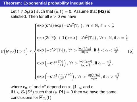
Theorem: Exponential probability inequalities

Let f ∈ Bb(S) such that (µ, f ) = 0. Assume that (H2) issatisfied. Then for all δ > 0 we have

P(

MTr (f ) > δ)≤

exp (c′′δ) exp(−c′δ2|Tr |

), ∀r ∈ N, if α < 1

2

exp (2c′δ(r + 1)) exp(−c′δ2|Tr |

), ∀r ∈ N, if α = 1

2

exp(−c′δ2|Tr |

), ∀r > log(δ/c0)

log α , if 12 < α <

√2

2

exp(−c′δ2 |Tr |

r+1

), ∀r > log(c0/δ)

log√

2, if α =

√2

2 ,

exp(−c′δ2

( 1α2

)r+1)

, ∀r > log(δ/c0)log α , if α >

√2

2

(6)

where c0, c′ and c′′ depend on α, ‖f‖∞ and c.

If f ∈ Bb(S3)

such that (µ, Pf ) = 0 then we have the sameconclusions for MTr (f ).

Theorem: Exponential probability inequalities

Let f ∈ Bb(S) such that (µ, f ) = 0. Assume that (H2) issatisfied. Then for all δ > 0 we have

P(

MTr (f ) > δ)≤

exp (c′′δ) exp(−c′δ2|Tr |

), ∀r ∈ N, if α < 1

2

exp (2c′δ(r + 1)) exp(−c′δ2|Tr |

), ∀r ∈ N, if α = 1

2

exp(−c′δ2|Tr |

), ∀r > log(δ/c0)

log α , if 12 < α <

√2

2

exp(−c′δ2 |Tr |

r+1

), ∀r > log(c0/δ)

log√

2, if α =

√2

2 ,

exp(−c′δ2

( 1α2

)r+1)

, ∀r > log(δ/c0)log α , if α >

√2

2

(6)

where c0, c′ and c′′ depend on α, ‖f‖∞ and c.If f ∈ Bb

(S3)

such that (µ, Pf ) = 0 then we have the sameconclusions for MTr (f ).


ideas for the proof

Chernoff inequality + successive conditioning and successiveapplications of Azuma-Bennet-Hoeffding using (H2).

• Once again, notice that the dichotomy around α = 12 and

α2 = 12 in (6) naturally appears from the calculations.


ideas for the proof

Chernoff inequality

+ successive conditioning and successiveapplications of Azuma-Bennet-Hoeffding using (H2).




ideas for the proof





ideas for the proof





Moderate deviation principle for MTr (f )

Let (bn) be an increasing sequence of positive real numberssuch that

(I) bn√n−→ +∞,

(II) if α2 < 12 , the sequence (bn) is such that

bn

n−→ 0,

(III) if α2 = 12 , the sequence (bn) is such that

bn log nn

−→ 0,

(IV) if α2 > 12 , the sequence (bn) is such that

bnαrn+1

√n

−→ 0.

• The conditions (II)-(IV) come from deviation inequalities(6).




(I) bn√n−→ +∞,


bn

n−→ 0,


bn log nn

−→ 0,


bnαrn+1

√n

−→ 0.





(I) bn√n−→ +∞,


bn

n−→ 0,


bn log nn

−→ 0,


bnαrn+1

√n

−→ 0.




Let f ∈ Bb(S3) such that Pf = 0. (Zr ) =(

1b|Tr |

MTr (f ))

Theorem (Moderate deviation principle)

Assume that (H2) is satisfied. Let (bn) be a sequence of realnumbers satisfying the above assumptions (I)-(IV), then (Zr )

satisfies a MDP in R with the speedb2|Tr ||Tr | and rate function

I(x) = x2

2(µ,Pf 2).

Particularly, for all δ > 0, we have

limr→∞

|Tr |b2|Tr |

log P(

1b|Tr |

|M|Tr |(f )| > δ

)= −I(δ). (7)

P(

1bTr

|MTr (f )| ≥ δ

)∼ exp

(−

b2Tr

Tr

δ2

2(µ, Pf 2)

)(7′)




1b|Tr |

MTr (f ))




I(x) = x2

2(µ,Pf 2).


limr→∞

|Tr |b2|Tr |

log P(

1b|Tr |

|M|Tr |(f )| > δ

)= −I(δ). (7)

P(

1bTr

|MTr (f )| ≥ δ

)∼ exp

(−

b2Tr

Tr

δ2

2(µ, Pf 2)

)(7′)




1b|Tr |

MTr (f ))




I(x) = x2

2(µ,Pf 2).


limr→∞

|Tr |b2|Tr |

log P(

1b|Tr |

|M|Tr |(f )| > δ

)= −I(δ). (7)

P(

1bTr

|MTr (f )| ≥ δ

)∼ exp

(−

b2Tr

Tr

δ2

2(µ, Pf 2)

)(7′)


Outline

1 Introduction

2 Goals


4 Results

5 Application


We consider the BAR(1) process

L(X1) = ν, and∀n ≥ 1,

X2n = α0Xn + β0 + ε2n

X2n+1 = α1Xn + β1 + ε2n+1,

The noise values in a compact set.F = Cb(R)(H2) are automatically satisfied with α = max(|α0|, |α1|).The least square estimator θr =

(αr

0, βr0, α

r1, β

r1

)of

θ = (α0, β0, α1, β1) is given by, for η ∈ 0, 1

αrη =

|Tr |−1 ∑i∈Tr

Xi X2i+η−(|Tr |−1 ∑

i∈Tr

Xi

)(|Tr |−1 ∑

i∈Tr

X2i+η

)

|Tr |−1∑

i∈Tr

X 2i −(|Tr |−1

∑i∈Tr

Xi

)2

βrη = |Tr |−1 ∑

i∈Tr

X2i+η − αrη|Tr |−1 ∑

i∈Tr

Xi .

(8)



L(X1) = ν, and∀n ≥ 1,

X2n = α0Xn + β0 + ε2n

X2n+1 = α1Xn + β1 + ε2n+1,

The noise values in a compact set.

F = Cb(R)(H2) are automatically satisfied with α = max(|α0|, |α1|).The least square estimator θr =

(αr

0, βr0, α

r1, β

r1

)of


αrη =

|Tr |−1 ∑i∈Tr

Xi X2i+η−(|Tr |−1 ∑

i∈Tr

Xi

)(|Tr |−1 ∑

i∈Tr

X2i+η

)

|Tr |−1∑

i∈Tr

X 2i −(|Tr |−1

∑i∈Tr

Xi

)2

βrη = |Tr |−1 ∑

i∈Tr


i∈Tr

Xi .

(8)



L(X1) = ν, and∀n ≥ 1,

X2n = α0Xn + β0 + ε2n

X2n+1 = α1Xn + β1 + ε2n+1,

The noise values in a compact set.F = Cb(R)

(H2) are automatically satisfied with α = max(|α0|, |α1|).The least square estimator θr =

(αr

0, βr0, α

r1, β

r1

)of


αrη =

|Tr |−1 ∑i∈Tr

Xi X2i+η−(|Tr |−1 ∑

i∈Tr

Xi

)(|Tr |−1 ∑

i∈Tr

X2i+η

)

|Tr |−1∑

i∈Tr

X 2i −(|Tr |−1

∑i∈Tr

Xi

)2

βrη = |Tr |−1 ∑

i∈Tr


i∈Tr

Xi .

(8)



L(X1) = ν, and∀n ≥ 1,

X2n = α0Xn + β0 + ε2n

X2n+1 = α1Xn + β1 + ε2n+1,

The noise values in a compact set.F = Cb(R)(H2) are automatically satisfied with α = max(|α0|, |α1|).

The least square estimator θr =(αr

0, βr0, α

r1, β

r1

)of


αrη =

|Tr |−1 ∑i∈Tr

Xi X2i+η−(|Tr |−1 ∑

i∈Tr

Xi

)(|Tr |−1 ∑

i∈Tr

X2i+η

)

|Tr |−1∑

i∈Tr

X 2i −(|Tr |−1

∑i∈Tr

Xi

)2

βrη = |Tr |−1 ∑

i∈Tr


i∈Tr

Xi .

(8)



L(X1) = ν, and∀n ≥ 1,

X2n = α0Xn + β0 + ε2n

X2n+1 = α1Xn + β1 + ε2n+1,

The noise values in a compact set.F = Cb(R)(H2) are automatically satisfied with α = max(|α0|, |α1|).The least square estimator θr =

(αr

0, βr0, α

r1, β

r1

)of


αrη =

|Tr |−1 ∑i∈Tr

Xi X2i+η−(|Tr |−1 ∑

i∈Tr

Xi

)(|Tr |−1 ∑

i∈Tr

X2i+η

)

|Tr |−1∑

i∈Tr

X 2i −(|Tr |−1

∑i∈Tr

Xi

)2

βrη = |Tr |−1 ∑

i∈Tr


i∈Tr

Xi .

(8)


µ1 : Θ → R and µ2 : Θ× R∗+ → R by writing

(µ, x) = µ1(θ) and (µ, x2) = µ2(θ, σ2), (9)

where θ = (α0, β0, α1, β1) ∈ Θ = (−1, 1)× R× (−1, 1)× R, andµ is the stationary distribution of Q.

Theorem

∀δ > 0 and ∀γ < min(

c1b1+δ , c1b

1+√

δ, c1b

1+ 4√δ

), where c1 = c1(µ1, µ2)

we have P(∥∥∥θr − θ

∥∥∥ > δ)≤

exp(c′′(γδ)1−p/2

)exp

(−c′(γδ)2−p|Tr |

), ∀r ∈ N, if α < 1

2

exp(c′(γδ(r + 1))1−p/2

)exp

(−c′(γδ)2−p|Tr |

), ∀r ∈ N, if α = 1

2

exp(−c′(γδ)2−p|Tr |

), ∀r >

log((γδ)1−p/2/c0)log α , if 1

2 < α <√

22

exp(−c′(γδ)2−p |Tr |

r+1

), ∀r >

log(c0/(γδ)1−p/2)log

√2

, if α =√

22

exp(−c′(γδ)2−p

( 1α2

)r+1)

, ∀r >log((γδ)1−p/2/c0)

log α , if α >√

22 ,

(10)

where c′ and c′′ depend on α, ‖f‖∞ and c, c0 depends on α,‖f‖∞, c and γ, and p ∈ 0, 1, 3/2.


End.

Documents

Deviation inequalities and moderate deviation principle ...reynaudb/jps/ergolim/BPSV_CIRM_2012.pdf · Université Blaise Pascal ... Figure: Cell division from E. J. Stewart and al