DevelopmentofanonlinearFiniteElementbeam model for dynamic ...publications.lib.chalmers.se/records/fulltext/142971.pdf · The ber model, which is based on a dynamic co-rotational

Development of a nonlinear Finite Element beammodel for dynamic contact problems applied topaper formingMaster’s Thesis in Solid and Fluid Mechanics

ERIK SVENNING

Fraunhofer Chalmers CentreDepartment of Computational Engineering and DesignCHALMERS UNIVERSITY OF TECHNOLOGYGoteborg, Sweden 2011Master’s Thesis 2011:05

MASTER’S THESIS 2011:05

Development of a nonlinear Finite Element beam model for

dynamic contact problems applied to paper forming

Master’s Thesis in Solid and Fluid MechanicsERIK SVENNING

Fraunhofer Chalmers CentreDepartment of Computational Engineering and Design

CHALMERS UNIVERSITY OF TECHNOLOGY

Goteborg, Sweden 2011

Development of a nonlinear Finite Element beam model for dynamic contact problemsapplied to paper forming

c©ERIK SVENNING, 2011

Master’s Thesis 2011:05ISSN 1652-8557Fraunhofer Chalmers CentreDepartment of Computational Engineering and DesignChalmers University of TechnologySE-412 96 GoteborgSwedenTelephone: + 46 (0)31-772 1000

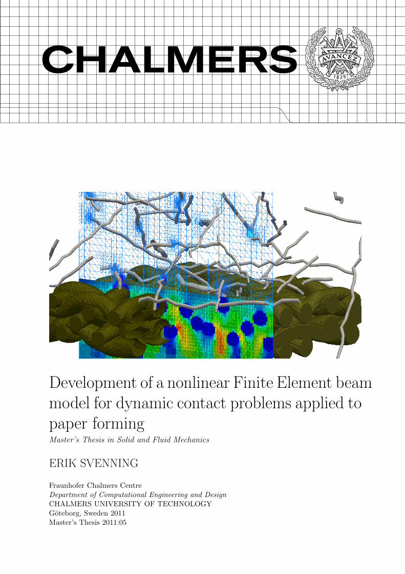
Cover:Paper fibers falling down onto a forming fabric. The wireframe shows the grid refinementsaround the fibers and the forming fabric. The slice is colored by the fluid velocity. Formingfabric geometry courtesy of Albany International.

Chalmers ReproserviceGoteborg, Sweden 2011

Finite element computations of the dynamic impact and contact of interacting bodies arenotoriously difficult.

F. Cirak and M. West, 2005

, FCC, Master’s Thesis 2011:05 5

Development of a nonlinear Finite Element beam model for dynamic contact problemsapplied to paper formingMaster’s Thesis in Solid and Fluid MechanicsERIK SVENNINGFraunhofer Chalmers CentreDepartment of Computational Engineering and DesignChalmers University of Technology

Abstract

A Finite Element model for simulation of paper forming has been developed andvalidated. Paper forming is the first step in the paper machine where a fiber sus-pension leaves the headbox and flows through a forming fabric. The fibers land onthe fabric and start to form the fiber web. Understanding this process is importantfor the development of better paper products, because the orientation and distri-bution of the individual fibers during this step have a large influence on the finalquality. Simulation of paper forming offers great challenges since it involves struc-tures with large displacements and large rotations, flow with complex boundaries,fluid-structure interaction with strong coupling and dynamic collisions.

The fiber model, which is based on a dynamic co-rotational formulation of theEuler-Bernoulli beam equation, accounts for geometric nonlinearities under the as-sumption of small strains. Two contact models have been implemented, a penaltymethod and the impulse based method Decomposition Contact Response. Thesemodels can handle fiber-fiber collisions as well as collisions between fibers and theforming fabric, which may have arbitrary geometry. Friction is included in the mod-els and elastic/inelastic collisions are accounted for with the coefficient of restitution.The fiber model was implemented in C++ and the nonlinear system of equations wassolved with Newton’s method. The flow around the fibers was simulated with theCFD software IBOFlow developed at FCC. IBOFlow is based on a finite volume dis-cretization on a Cartesian octree grid that can be dynamically refined and coarsened.The flow around the moving fibers is resolved and the Hybrid Immersed BoundaryMethod is used to model the presence of fibers in the flow.

Extensive validation of the implementation has been performed against severaldemanding test cases from the literature. These cases include static instability withpostbuckling, large amplitude oscillation of slender structures and dynamic impacts.Large effort was dedicated to making the code robust and efficient.

The code was used to study two fluid-structure interaction problems. First, asingle fiber oscillating in a cross flow was studied and the numerical results werecompared to an analytical solution obtained from a Fourier series expansion of theEuler-Bernoulli beam equation. Paper forming with two forming fabrics of differentgeometry was also studied. A qualitative comparison of the resulting distributionand orientation of paper fibers was made.

Keywords: paper forming, fluid-structure interaction, FEM, contact modeling, ImmersedBoundary Methods

, FCC, Master’s Thesis 2011:05 I

II , FCC, Master’s Thesis 2011:05

Contents

Abstract I

Contents III

Preface V

Notations VI

1 Introduction 11.1 Purpose . . . . . . . . . . . . . . . . . . . . . . . . . . . . . . . . . . . . . 11.2 Limitations . . . . . . . . . . . . . . . . . . . . . . . . . . . . . . . . . . . 21.3 Approach . . . . . . . . . . . . . . . . . . . . . . . . . . . . . . . . . . . . 21.4 Review of beam models . . . . . . . . . . . . . . . . . . . . . . . . . . . . . 21.5 Review of contact models . . . . . . . . . . . . . . . . . . . . . . . . . . . 4

1.5.1 Penalty methods . . . . . . . . . . . . . . . . . . . . . . . . . . . . 41.5.2 Lagrange multipliers . . . . . . . . . . . . . . . . . . . . . . . . . . 61.5.3 Impulse based methods . . . . . . . . . . . . . . . . . . . . . . . . . 7

2 Theory 82.1 Fluid model . . . . . . . . . . . . . . . . . . . . . . . . . . . . . . . . . . . 8

2.1.1 Fluid-structure coupling . . . . . . . . . . . . . . . . . . . . . . . . 92.1.2 Simplified alternative for fluid-structure coupling . . . . . . . . . . 112.1.3 Treatment of complex boundaries . . . . . . . . . . . . . . . . . . . 112.1.4 CFD solver used in the present work . . . . . . . . . . . . . . . . . 11

2.2 Fiber model . . . . . . . . . . . . . . . . . . . . . . . . . . . . . . . . . . . 122.2.1 Geometry of a fiber . . . . . . . . . . . . . . . . . . . . . . . . . . . 122.2.2 Small rotation FE formulation . . . . . . . . . . . . . . . . . . . . . 152.2.3 Mathematics of finite rotations . . . . . . . . . . . . . . . . . . . . 172.2.4 Computation of element deformations . . . . . . . . . . . . . . . . . 182.2.5 Large rotation Finite Element formulation . . . . . . . . . . . . . . 192.2.6 Dynamic FE formulation . . . . . . . . . . . . . . . . . . . . . . . . 21

2.3 Contact detection . . . . . . . . . . . . . . . . . . . . . . . . . . . . . . . . 222.3.1 Spatial search - identifying segments that are close to each other . . 232.3.2 Distance between a segment and a fixed point . . . . . . . . . . . . 232.3.3 Distance between two segments . . . . . . . . . . . . . . . . . . . . 26

2.4 Contact models . . . . . . . . . . . . . . . . . . . . . . . . . . . . . . . . . 282.4.1 A penalty method suitable for paper forming . . . . . . . . . . . . . 282.4.2 Decomposition Contact Response . . . . . . . . . . . . . . . . . . . 29

2.4.2.1 DCR for fiber-fiber contact . . . . . . . . . . . . . . . . . 312.4.2.2 DCR for fiber-fabric contact . . . . . . . . . . . . . . . . . 32

2.5 Measures of fiber web properties . . . . . . . . . . . . . . . . . . . . . . . . 322.5.1 Mass distribution (Grammage) . . . . . . . . . . . . . . . . . . . . 322.5.2 Fiber directions (anisotropy) . . . . . . . . . . . . . . . . . . . . . . 33

3 Numerical results 343.1 Validation of FE solver . . . . . . . . . . . . . . . . . . . . . . . . . . . . . 34

3.1.1 Validation of static problems . . . . . . . . . . . . . . . . . . . . . . 343.1.1.1 Hockling of a cable . . . . . . . . . . . . . . . . . . . . . . 343.1.1.2 Lateral buckling of a hinged frame . . . . . . . . . . . . . 37

, FCC, Master’s Thesis 2011:05 III

3.1.2 Validation of dynamic problems . . . . . . . . . . . . . . . . . . . . 403.1.2.1 Free vibration of right-angle cantilever beam . . . . . . . . 403.1.2.2 Vibration of a cantilever beam with twisted cross section . 44

3.1.3 Validation of problems involving contact . . . . . . . . . . . . . . . 493.1.3.1 Collision of two rods . . . . . . . . . . . . . . . . . . . . . 493.1.3.2 Impact between spinning rod and table . . . . . . . . . . . 51

3.2 Fluid-Structure Interaction without contact . . . . . . . . . . . . . . . . . 543.2.1 Oscillating cantilever beam in cross flow . . . . . . . . . . . . . . . 54

3.3 Simulations of paper forming . . . . . . . . . . . . . . . . . . . . . . . . . . 603.3.1 Problem description . . . . . . . . . . . . . . . . . . . . . . . . . . 603.3.2 Laydown simulation . . . . . . . . . . . . . . . . . . . . . . . . . . 633.3.3 Qualitative comparison of two forming fabrics . . . . . . . . . . . . 67

4 Summary and Conclusions 72

5 Further work 73

A Formulas for three-dimensional rotations 76

B Formulas for the static co-rotational formulation 76B.1 Γ . . . . . . . . . . . . . . . . . . . . . . . . . . . . . . . . . . . . . . . . . 76B.2 P . . . . . . . . . . . . . . . . . . . . . . . . . . . . . . . . . . . . . . . . . 78B.3 F . . . . . . . . . . . . . . . . . . . . . . . . . . . . . . . . . . . . . . . . . 78

C Fourier series expansion of an oscillating cantilever beam in a fluid 78

D Jacobian of inertia force 81

E Shortest unsigned distance between two segments 84

IV , FCC, Master’s Thesis 2011:05

Preface

This thesis is submitted in partial fulfillment of the requirements for the MSc degree fromChalmers University of Technology. The work was carried out during the period fromJanuary 2011 to June 2011 at Fraunhofer Chalmers Centre (FCC). Professor KennethRunesson at the Department of Applied Mechanics, Division of Material & ComputationalMechanics was examiner and Bjorn Andersson at FCC was supervisor.

Acknowledgements

This work was part of the ISOP project with industrial partners Albany International,Eka Chemicals, Stora Enso and Tetra Pak. It was supported in part by the SwedishFoundation for Strategic Research (SSF) through the Gothenburg Mathematical ModelingCentre (GMMC).

I wish to thank the colleagues at FCC for the great atmosphere. I especially want tothank my supervisor Bjorn Andersson for encouraging support, fruitful discussions andgreat help with programming. I would also like to thank my examiner Professor KennethRunesson. A special thanks to Dr. Andreas Mark for sharing his expertise in CFD, forteaching me high performance computing and for always keeping his door open. I wouldlike to thank Assoc. Professor Fredrik Edelvik for his faith in me and for giving me thepossibility to work with this interesting project. Thanks to Dr. Robert Bohlin for helpwith quaternions and to Assoc. Professor Mats Jirstrand for help with Mathematica. Myfellow student Anton Berce is greatfully acknowledged for sharing his knowledge aboutpaper machines and for the good discussions about work and life.

Finally, I would like to thank Annie for her love and support.

Goteborg June 2011Erik Svenning

, FCC, Master’s Thesis 2011:05 V

Nomenclature

δu Infinitesimal change in u

δDirac Dirac delta function

δij Kronecker delta

λ Lagrangian multiplier

µfr Coefficient of friction

ν Poisson’s ratio

u An overbar indicates the deformational part of a quantity.

ρ Density

ω Spin axis

θ Angle

A Angular acceleration

ex, ey, ez Base vectors in the current configuration.

f Force

n Unit normal

pe Subscript e indicates a variable associated with the end point of an element.

ps Subscript s indicates a variable associated with the start point of an element.

ploc Subscript loc indicates a variable expressed in local coordinates.

q Vector that rotates with the major axis of the cross section.

t Unit tangent

uel The superscript el indicates that the variable is associated with an element.

vrel Relative velocity

w Angular velocity

Ω Spin tensor

E Change of coordinates matrix. The base vectors in the current configuration are thecolumns of E.

Iρ Inertia tensor

T Rotation tensor

Tg Subscript or superscript g denotes a variable expressed in global coordinates.

Γ Matrix that relates the rotation of the element frame to the displacements androtations at the element nodes.

VI , FCC, Master’s Thesis 2011:05

B Matrix containing the derivatives of the base functions.

F Matrix used in the computation of the geometric stiffness. F is a function of theinternal force vector only.

H Matrix that transforms the tangent stiffness and internal force vector from anglesto spin variables.

K Tangent stiffness matrix

M Mass matrix

P Projector matrix

Ψ Rotational pseudovector

p Momentum

ϕ Twisting angle of undeformed cross section

cd Drag coefficient

E Young’s modulus

ecor Coefficient of restitution

fn Normal force

g Gap function

i Index: i = 1, 2, 3; Einstein’s summation convention is used where summation isimplied over repeated indices unless otherwise stated.

L Length of undeformed segment.

l Length of deformed segment.

M Bending moment

Ra Radius of major axis of the elliptical cross section

Rb Radius of minor axis of the elliptical cross section

S () Spin operator

V Potential energy

, FCC, Master’s Thesis 2011:05 VII

VIII , FCC, Master’s Thesis 2011:05

1 Introduction

Paper forming is the first step in the paper machine where a fiber suspension leaves theheadbox and flows through a forming fabric. The fibers land on the fabric and start toform the fiber web. Understanding this process is important for the development of betterpaper products, because the orientation and distribution of the individual fibers duringthis step have a large influence on the final paper quality.

Simulation of this process offers huge challenges since it involves transient fluid flowwith many immersed solid objects subjected to large displacements. The problem involvesfluid structure interaction with strong coupling: the immersed objects are forced to followthe fluid, but the fluid is also strongly influenced by the immersed objects. The effectof strong coupling can be described by throwing a ball in air and water. The trajectoryof a ball thrown in air can be described relatively accurate even without considering thesurrounding fluid, the coupling is quite weak and the weak coupling makes the problemeasier. The trajectory of a ball thrown in water is much more difficult to predict, the waterwill have a very strong influence on the motion of the ball. The difficulty of the problemis influenced by how heavy the ball is compared to the fluid. The ball is heavy comparedto the air, which makes the case of a ball in air easy. When compared to water, the weightof the ball is relatively low. As a result, the motion of the ball is influenced more by thefluid forces than by its own inertia. This effect makes the formulation of the fluid-structurecoupling important and the problem becomes difficult. The problem becomes very difficultwhen the object has the same density as the fluid. When this occurs, the object is said tobe buoyant. Paper fibers in water are buoyant.

Strong coupling is not the only challenge in simulations of paper forming, contactphenomena play an important role when the fibers fall down onto the forming fabric.Contact forces with friction keep the fibers from falling off the forming fabric and beeingcarried away by the flow. The number of contacts increases as more and more fibers laydown on top of the fiber web. Since the fiber web is kept together by contact forces, veryrobust modeling of contacts is required.

Understanding the phenomena governing paper forming requires DNS simulations wherethe coupling between the fluid and the solid objects is handled properly and the flow aroundevery fiber is resolved. Simulations of fibers described in the literature use drag correlationsinstead of resolving the flow around the individual fibers and model the fibers as chains ofspheres or rigid rods instead of employing rigorous beam models that are normally usedto study slender structures. Therefore, an implementation of more accurate methods isnecessary.

1.1 Purpose

The goal of the project is to develop a model that can be used to study initial paperforming. To achieve this, a nonlinear Finite Element beam model with collisions is required.Therefore, the goal of this thesis consists of two parts:

• Implement and validate a Finite Element code for simulation of paper fibers. Themodel must be rigorous and derived from fundamental laws of continuum mechanics.The code must be fast and robust. In order to ensure that the implementationis correct and physically sound, the code should be validated against demandingstructural dynamics problems described in the literature.

• Show that the code can be used to simulate paper forming. Especially, it must beshown that the code can handle a large number of interacting fibers without stabilityproblems.


1.2 Limitations

The project is mainly restricted in the following directions:

• Linear elastic material is assumed, other constitutive models are not considered.

• Initial simulations of paper forming are performed in order to demonstrate the capa-bilities of the code. However, there are not enough computational resources availableto perform a full set of simulations of paper forming.

• Two contact models are implemented and compared. It is not the purpose of thisproject to implement all possible classes of contact algorithms.

• It is not the purpose of this project to investigate the effects of turbulence on theprocess.

1.3 Approach

FCC’s in-house CFD code IBOFlow [16] (Immersed Boundary Octree Flow solver) is usedto simulate the fluid flow around the paper fibers. Geometrical descriptions of formingfabrics and paper fibers are generated with GeoDict [10]. A Finite Element fiber modelbased on a co-rotational formulation of the Euler-Bernoulli beam equation is implemented.Two contact models are also implemented and included in the Finite Element model anddemanding test problems from the literature are chosen for validation of the fiber code.The FE code is coupled with the CFD code, resulting in a simulation software capableof handling fluid-structure interaction with strong coupling and dynamic impacts betweenthe solid objects. The Immersed Boundary Method is used to resolve the flow around thefibers, while the forming fabrics are described numerically with voxelizations.

A simple drag correlation with one-way coupling was also implemented. The resultsobtained from these simplified simulations should be interpreted carefully, but this optiongives the possibility to show that the FE code can handle a large number of fibers withoutstability problems. It is also shown that relevant postprocessing data can be extractedfrom the simulations and a qualitative comparison between two forming fabrics is made.

The code is written in C++ and generic high performance libraries are used for distancesearches, matrix computations and solution of the large and sparse system of equations.The open source program Paraview is used for 3D visualizations and Matlab is used todraw 2D plots.

1.4 Review of beam models

Beams are slender objects characterized by the fact that one dimension is much larger thanthe other two dimensions. Many researches have derived equations governing the dynamicmotion of such objects. Two widely used examples are the Euler-Bernoulli beam theoryand the Timoshenko beam theory [12]. In the classical, small displacement formulation, theEuler-Bernoulli beam equation includes the effect of translational inertia, but it neglectsthe effect of rotational inertia. Bending is included in the strain energy, but shearing isnot. The Timoshenko beam equation includes rotational inertia as well as shearing in thecross section. It does, however, assume small rotations and small strains. Both the Euler-Bernoulli and the Timoshenko beam theories are good approximations for slender beamsoscillating at low frequencies, but the Timoshenko beam theory is a better approximationfor non-slender beams and high frequencies. In simulations of paper forming, the paperfibers will be transported by the fluid flow field and may be subjected to large displacements

2 , FCC, Master’s Thesis 2011:05

as well as large (finite) rotations. The Euler-Bernoulli and Timoshenko beam theories aspresented in [12] do not allow finite rotations and therefore these models can not be usedwithout modification. Han et al. [12] also discuss the Rayleigh beam theory and the Shearbeam theory. These models suffer from the same fundamental weakness, they do not allowfinite rotations.

Ibrahimbegovic and Mikdad [17] derived a beam model based on the Reissner beamtheory. The model is geometrically exact and it is capable of handling finite strains as wellas finite rotations. Different ways of parametrizing large rotations were discussed.

Simo and Vu-Quoc [29] derived a fully nonlinear, geometrically exact beam model. Themodel is capable of handling finite strains as well as finite rotations. Several numericalexamples were given and the computational aspects of the implementation were discussed.

Nour-Omid and Rankin [25] derived a co-rotational formulation which can be used toextend a linear Finite Element model so that finite rotations are allowed. The funda-mental idea of the co-rotational approach is that the linear equations are formulated ina co-rotational frame which moves with the element. In this way, finite rotations can beallowed even if the original Finite Element model assumes small rotations. The consistentlinearization of the co-rotational formulation results in a projector matrix, which is used tomodify the linear element model. The model proposed in [25] is derived for static problems.

Crisfield, Galvanetto and Jelenic [5] studied the dynamics of co-rotational beams sub-jected to finite rotations. The weak form of the inertia terms was derived and differenttime stepping schemes were discussed.

Several authors interested in the motion of fibers in a fluid flow have modeled fibers asa chain of spheres or rods. One example is the model proposed by Lindstrom and Uesaka[18, 19, 20], where fibers are treated as a chain of rigid rods connected with springs. Thederivation of the model proposed in [19] starts with Newton’s second law for linear andangular momentum. The fibers are considered to be inextensible, but the inextensibilityconstraint is neither enforced with Lagrangian multipliers nor with an axial stiffness in thesetting of a penalty method. Instead, a constraint on the velocity in the joints betweenthe segments is proposed. However, no discussion is given on how the resulting constraintforce is computed or how it enters the equation of motion.

The equations in the models proposed by Crisfield et al. [5], Ibrahimbegovic andMikdad [17], Nour-Omid and Rankin [25] and Simo and Vu-Quoc [29] are solved withNewton’s method. Therefore second order convergence of the iterations is obtained withthese models, so that an accurate solution is obtained after just a few iterations. Further-more, Newton’s method is very robust, so that these models will converge even in caseswhere strong nonlinearities occur. It is unclear if Lindstrom and Uesaka [19] use Newton’smethod.

A beam model suitable for simulation of paper fibers must allow finite rotations. Theclassical theories described in [12] do not fulfill this criterion without modification. It isdesirable to use a fiber model based on a beam theory. Therefore, three possible choicesremain: the finite strain Reissner beam model proposed by Ibrahimbegovic and Mikdad[17], the finite strain beam model proposed by Simo and Vu-Quoc [29] and the finite rota-tion co-rotational formulation proposed by Nour-Omid and Rankin [25] with inertia termscomputed according to Crisfield et al. [5]. Paper fibers falling down onto a forming fabricwill be subjected to large rotations, but the strain will be small or moderate. Therefore,the extra complexity in [17] and [29] needed to allow finite strains is not necessary for thepurpose of the present work.

The models in [17], [25] and [29] are all physically sound models that would be suitablefor simulations of paper forming. The co-rotational approach described by Nour-Omid andRankin [25] with inertia accounted for as described by Crisfield et al. [5] is the simplest


model that fulfills the requirements for simulation of paper fibers. Therefore, this modelis chosen for the implementation in the present work.

1.5 Review of contact models

The contact models described in the literature can roughly be divided into three classes ofalgorithms [13]: penalty methods, methods based on Lagrangian multipliers and impulse-based methods. All three classes of contact models suffer from different kinds of numericalproblems. There is no perfect contact model that works well for all types of problems,the choice of contact model will depend on the properties of the problem studied and thedesired level of detail of the simulation. This section gives a short overview of the differenttypes of contact models available.

In the following, the overlap is characterized by the gap function g, which measures thepenetration in the normal direction of the contacting surfaces.

1.5.1 Penalty methods

Penalty methods allow the elements to overlap and add a repulsive force which increaseswith increasing overlap. Explicitly adding a contact force which depends on the magnitudeof the overlap is the fundamental idea of this algorithm and this idea is used in all differentformulations of penalty methods. The difference between different penalty methods ishow this repulsive force is computed. Wriggers [32] added a quadratic term to the energypotential, resulting in a penalty force that varies linearly with the overlap. This approachis energy conserving, all collisions are considered to be elastic. Crowe, Sommerfeld andTsuji [6] use a penalty force based on Hertzian contact theory for spheres of equal size,where the normal force is given by:

fn = −f0 (−g (x))1.5 − ηvrel · n (1.1)

Here, f0 is the normal stiffness and the Hertzian theory is extended with dissipation char-acterized by a damping coefficent η. This approach allows modeling of collisions that arenot completely elastic, but the relation between η and the coefficient of restitution ecor isnot trivial. A relation between η and ecor for a sphere is given in [6]. However, it thatrelation η depends on the mass of the sphere as well as the overlap. Since η depends onthe configuration of the system, it can no longer be interpreted as a constant materialparameter.

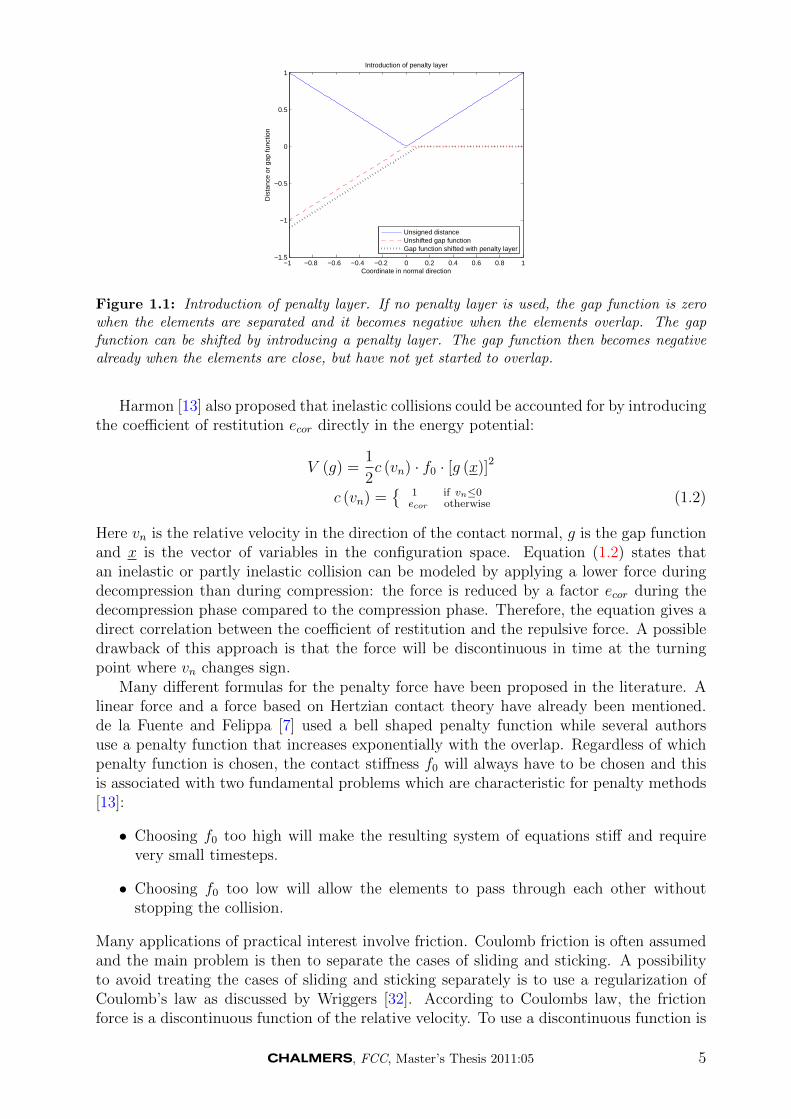
Harmon [13] proposed several extensions to penalty methods in his PhD thesis. Onesuch modification is the introduction of penalty layers. The gap function g is usuallydefined in such a way that g = 0 when the distance between the impacting elements iszero and g < 0 when the elements are overlapping. It is possible to shift the gap functionso that g = 0 when the distance between the elements is small but not zero. The gapfunction then becomes negative when the distance is exactly zero. The idea of a shiftedgap function is visualized in figure (1.1). In this way, a penalty force can be applied whenthe elements are close rather than actually overlapping. Harmon [13] suggests using thisapproach for cases where the geometrical effects of overlap are difficult to repair. Such acase occurs when the geometry of the problem is complicated. In this case, it is fairly easyto determine the distance from a point to a surface, but it could be difficult to determine ifthe point is outside the geometry or if it is inside the geometry so that overlap has occured.If this is a problem, a penalty layer can be applied to ensure that overlap never occurs inthe simulation.


−1 −0.8 −0.6 −0.4 −0.2 0 0.2 0.4 0.6 0.8 1−1.5

−1

−0.5

0

0.5

1Introduction of penalty layer

Coordinate in normal directionD

ista

nce

or g

ap fu

nctio

n

Unsigned distanceUnshifted gap functionGap function shifted with penalty layer

Figure 1.1: Introduction of penalty layer. If no penalty layer is used, the gap function is zerowhen the elements are separated and it becomes negative when the elements overlap. The gapfunction can be shifted by introducing a penalty layer. The gap function then becomes negativealready when the elements are close, but have not yet started to overlap.

Harmon [13] also proposed that inelastic collisions could be accounted for by introducingthe coefficient of restitution ecor directly in the energy potential:

V (g) =1

2c (vn) · f0 · [g (x)]2

c (vn) =

1 if vn≤0ecor otherwise (1.2)

Here vn is the relative velocity in the direction of the contact normal, g is the gap functionand x is the vector of variables in the configuration space. Equation (1.2) states thatan inelastic or partly inelastic collision can be modeled by applying a lower force duringdecompression than during compression: the force is reduced by a factor ecor during thedecompression phase compared to the compression phase. Therefore, the equation gives adirect correlation between the coefficient of restitution and the repulsive force. A possibledrawback of this approach is that the force will be discontinuous in time at the turningpoint where vn changes sign.

Many different formulas for the penalty force have been proposed in the literature. Alinear force and a force based on Hertzian contact theory have already been mentioned.de la Fuente and Felippa [7] used a bell shaped penalty function while several authorsuse a penalty function that increases exponentially with the overlap. Regardless of whichpenalty function is chosen, the contact stiffness f0 will always have to be chosen and thisis associated with two fundamental problems which are characteristic for penalty methods[13]:

• Choosing f0 too high will make the resulting system of equations stiff and requirevery small timesteps.

• Choosing f0 too low will allow the elements to pass through each other withoutstopping the collision.

Many applications of practical interest involve friction. Coulomb friction is often assumedand the main problem is then to separate the cases of sliding and sticking. A possibilityto avoid treating the cases of sliding and sticking separately is to use a regularization ofCoulomb’s law as discussed by Wriggers [32]. According to Coulombs law, the frictionforce is a discontinuous function of the relative velocity. To use a discontinuous function is


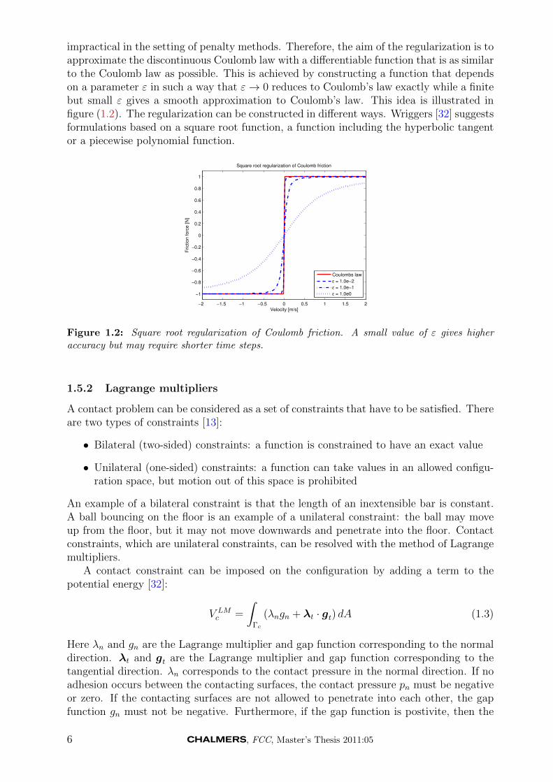
impractical in the setting of penalty methods. Therefore, the aim of the regularization is toapproximate the discontinuous Coulomb law with a differentiable function that is as similarto the Coulomb law as possible. This is achieved by constructing a function that dependson a parameter ε in such a way that ε→ 0 reduces to Coulomb’s law exactly while a finitebut small ε gives a smooth approximation to Coulomb’s law. This idea is illustrated infigure (1.2). The regularization can be constructed in different ways. Wriggers [32] suggestsformulations based on a square root function, a function including the hyperbolic tangentor a piecewise polynomial function.

−2 −1.5 −1 −0.5 0 0.5 1 1.5 2

−1

−0.8

−0.6

−0.4

−0.2

0

0.2

0.4

0.6

0.8

1

Velocity [m/s]

Frictio

n f

orc

e [

N]

Square root regularization of Coulomb friction

Coulombs law

ε = 1.0e−2

ε = 1.0e−1

ε = 1.0e0

Figure 1.2: Square root regularization of Coulomb friction. A small value of ε gives higheraccuracy but may require shorter time steps.

1.5.2 Lagrange multipliers

A contact problem can be considered as a set of constraints that have to be satisfied. Thereare two types of constraints [13]:

• Bilateral (two-sided) constraints: a function is constrained to have an exact value

• Unilateral (one-sided) constraints: a function can take values in an allowed configu-ration space, but motion out of this space is prohibited

An example of a bilateral constraint is that the length of an inextensible bar is constant.A ball bouncing on the floor is an example of a unilateral constraint: the ball may moveup from the floor, but it may not move downwards and penetrate into the floor. Contactconstraints, which are unilateral constraints, can be resolved with the method of Lagrangemultipliers.

A contact constraint can be imposed on the configuration by adding a term to thepotential energy [32]:

V LMc =

∫Γc

(λngn + λt · gt) dA (1.3)

Here λn and gn are the Lagrange multiplier and gap function corresponding to the normaldirection. λt and gt are the Lagrange multiplier and gap function corresponding to thetangential direction. λn corresponds to the contact pressure in the normal direction. If noadhesion occurs between the contacting surfaces, the contact pressure pn must be negativeor zero. If the contacting surfaces are not allowed to penetrate into each other, the gapfunction gn must not be negative. Furthermore, if the gap function is postivite, then the


contact pressure must be zero and if the contact pressure is not zero, then the gap functionmust be zero. Therefore, the contact pressure and normal gap function are subjected tothe Kuhn-Tucker-Karush conditions [32]:

gn ≥ 0 pn ≤ 0 gnpn = 0 on Γc (1.4)

In the equation above, Γc is the part of the boundary subjected to contact.Coulomb’s law can be used in the tangential direction and slip-stick behavior can be

enforced exactly without regularization. In order to do this, the cases of slip and stickmust be treated separately.

Many variants of the Lagrange multiplier method exist. The constraint equations canbe discretized either implicitly, enforcing the constraints at the end of the time step, orexplicitly, enforcing the constraints at the start of the time step [13]. Furthermore, per-turbed Lagrange formulations exist, where a Lagrange multiplier method is mixed with apenalty method [32].

The Lagrange multiplier method can be used for dynamic problems with perfectlyelastic collisions [3]. For such cases, the constraint equations can be formulated by requiringthat the overlap is zero at the end of the time step.

In order to model inelastic collisions with Lagrange multipliers, it would not suffice toadd a constraint on the displacement. In principle, a constraint could instead be added onthe velocity to ensure that the pre- and postcollisional velocities are related by the coeffi-cient of restitution. However, if a constraint on the velocity is imposed, the impenetrabilityconstraint on the displacement would have to be sacrificed.

1.5.3 Impulse based methods

A collision between two solid objects results in a high contact force during a short timeinterval. Instead of resolving the high force and the short time interval, the contact forcescan be treated as instantaneous forces, i.e. impulses [13]. Impulse based methods use thisapproach to predict a change in momentum due to the collision instead of predicting achange in acceleration.

One example is the Hard sphere model discussed in [6]. In that model, instantaneouscontact between two spheres is considered. Elastic and inelastic collisions are accountedfor with the coefficient of restitution ecor.There are two possible choices for the time stepping strategy in impulse based methods:

• Simulate until a collision occurs, resolve the collision and then simulate until the nextcollision occurs. An advantage of this approach is that geometry overlap will neveroccur, because the simulation is halted just before impact and the collision is resolvedbefore proceeding. A disadvantage is that there are cases when this algorithm willnot be able to reach the end time of the simulation tend in a finite number of timesteps because an infinite number of collisions occur before reaching that time [2].An example of this phenomenon is a ball with 0 < ecor < 1 bouncing on the floor.At each bounce, a fraction of the kinetic energy in the ball will be restituted andthe time to the next impact will be smaller than the time between the previous twoimpacts. As a result, the ball will hit the floor an infinite number of times beforecoming to rest. Chatterjee and Ruina [2] suggest that this problem could be handledwith extrapolation or truncation of the motion.

• Predictor-corrector steps: first take a time step with a predefined time step size,then resolve all the collisions that have occured during that time step. When allcollisions have been resolved, a new time step can be taken. If this approach is


chosen, some overlap must be allowed and this overlap must be handled in a robustway. The main advantage of this approach is that a fixed time step can be used andtherefore the number of time steps needed to simulate a given physical time intervalwill be known a-priori. An example of this approach is the Decomposition ContactResponse (DCR) algorithm proposed by Cirak and West [4]. This algorithm relies ona decomposition of the momentum p = M ·v into a normal and a tangential part. Thenormal direction is defined as the gradient of the constraint function: n = ∇g. Theimpulse in the normal direction is found by projecting p onto n = ∇g and from thisthe tangential impulse can be computed. When the impulse has been decomposedinto its normal and tangential parts, the coefficient of restitution ecor can be used toupdate the normal impulse and Coulomb’s law can be used to update the tangentialimpulse. This algorithm can handle the different cases of sliding and sticking withoutdifficulty.

2 Theory

2.1 Fluid model

The motion of an incompressible viscous fluid is governed by the Navier-Stokes equations:

∂uj∂xj

= 0 (2.1)

ρf∂

∂t(ui) + ρfuj

∂ui∂xj

= − ∂p

∂xi+

∂

∂xj

(µ∂ui∂xj

)+ ρggi (2.2)

In the equation above, ρf is the fluid density, ui is the velocity in coordinate directioni, p is the pressure, µ is the fluid viscosity and gi is the gravity. (2.1) is the continuityequation and (2.2) gives the momentum equations in the three coordinate direction. Thefour equations in (2.1) and (2.2) can be used to solve for the four unknowns: the threecomponents of the velocity and the pressure. The Navier-Stokes equations are nonlinearand coupled, note that each velocity component is present in all four equations. Therefore,the equations in (2.1) and (2.2) can not be used one by one to solve for one variable ata time. The equations can be solved simultaneously, or they can be rewritten to enablesolution of one equation at a time. The nonlinearity in the equations could be handledby solving them with e.g. Newton’s method or fix-point iterations. The widely used CFDcodes use fix-point iterations and solve the equations in a segregated way, thus solvingfor one variable at a time. Two problems must be handled to solve the equations in asegregated way. First, the coupling of the equations must be handled sufficiently well, sothat the iterative solution converges. The second problem is that the momentum equations(2.2) offer equations for the velocity components, but the continuity equation (2.1) can notbe used to solve for the pressure without modification. A popular way to solve (2.1) and(2.2) in a segregated way is to use the SIMPLE method and rewrite the continuity equationas an equation for pressure correction. The SIMPLE method can be summarized as follows[21]:

1. Solve the momentum equations (2.2) with a guessed pressure.

2. Solve the pressure correction equation.

3. Update the pressure with the computed pressure correction. Correct the velocity sothat continuity holds.


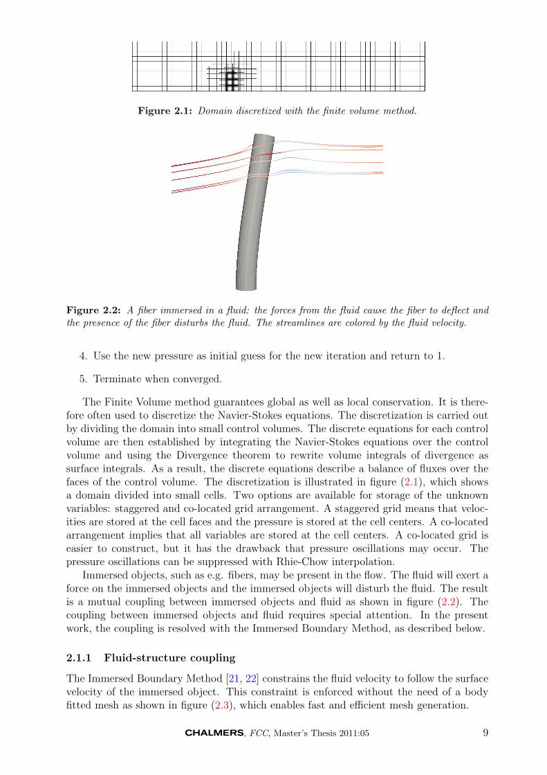
Figure 2.1: Domain discretized with the finite volume method.

Figure 2.2: A fiber immersed in a fluid: the forces from the fluid cause the fiber to deflect andthe presence of the fiber disturbs the fluid. The streamlines are colored by the fluid velocity.

4. Use the new pressure as initial guess for the new iteration and return to 1.

5. Terminate when converged.

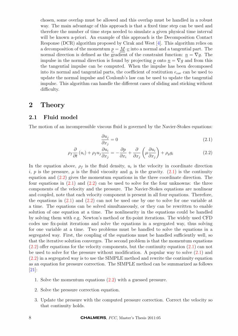
The Finite Volume method guarantees global as well as local conservation. It is there-fore often used to discretize the Navier-Stokes equations. The discretization is carried outby dividing the domain into small control volumes. The discrete equations for each controlvolume are then established by integrating the Navier-Stokes equations over the controlvolume and using the Divergence theorem to rewrite volume integrals of divergence assurface integrals. As a result, the discrete equations describe a balance of fluxes over thefaces of the control volume. The discretization is illustrated in figure (2.1), which showsa domain divided into small cells. Two options are available for storage of the unknownvariables: staggered and co-located grid arrangement. A staggered grid means that veloc-ities are stored at the cell faces and the pressure is stored at the cell centers. A co-locatedarrangement implies that all variables are stored at the cell centers. A co-located grid iseasier to construct, but it has the drawback that pressure oscillations may occur. Thepressure oscillations can be suppressed with Rhie-Chow interpolation.

Immersed objects, such as e.g. fibers, may be present in the flow. The fluid will exert aforce on the immersed objects and the immersed objects will disturb the fluid. The resultis a mutual coupling between immersed objects and fluid as shown in figure (2.2). Thecoupling between immersed objects and fluid requires special attention. In the presentwork, the coupling is resolved with the Immersed Boundary Method, as described below.

2.1.1 Fluid-structure coupling

The Immersed Boundary Method [21, 22] constrains the fluid velocity to follow the surfacevelocity of the immersed object. This constraint is enforced without the need of a bodyfitted mesh as shown in figure (2.3), which enables fast and efficient mesh generation.


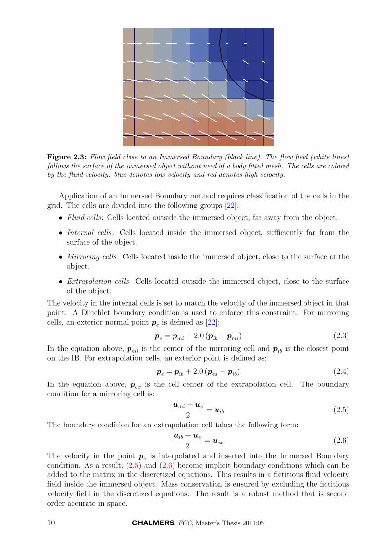
Figure 2.3: Flow field close to an Immersed Boundary (black line). The flow field (white lines)follows the surface of the immersed object without need of a body fitted mesh. The cells are coloredby the fluid velocity: blue denotes low velocity and red denotes high velocity.

Application of an Immersed Boundary method requires classification of the cells in thegrid. The cells are divided into the following groups [22]:

• Fluid cells : Cells located outside the immersed object, far away from the object.

• Internal cells : Cells located inside the immersed object, sufficiently far from thesurface of the object.

• Mirroring cells : Cells located inside the immersed object, close to the surface of theobject.

• Extrapolation cells : Cells located outside the immersed object, close to the surfaceof the object.

The velocity in the internal cells is set to match the velocity of the immersed object in thatpoint. A Dirichlet boundary condition is used to enforce this constraint. For mirroringcells, an exterior normal point pe is defined as [22]:

pe = pmi + 2.0 (pib − pmi) (2.3)

In the equation above, pmi is the center of the mirroring cell and pib is the closest pointon the IB. For extrapolation cells, an exterior point is defined as:

pe = pib + 2.0 (pex − pib) (2.4)

In the equation above, pex is the cell center of the extrapolation cell. The boundarycondition for a mirroring cell is:

umi + ue2

= uib (2.5)

The boundary condition for an extrapolation cell takes the following form:

uib + ue2

= uex (2.6)

The velocity in the point pe is interpolated and inserted into the Immersed Boundarycondition. As a result, (2.5) and (2.6) become implicit boundary conditions which can beadded to the matrix in the discretized equations. This results in a fictitious fluid velocityfield inside the immersed object. Mass conservation is ensured by excluding the fictitiousvelocity field in the discretized equations. The result is a robust method that is secondorder accurate in space.


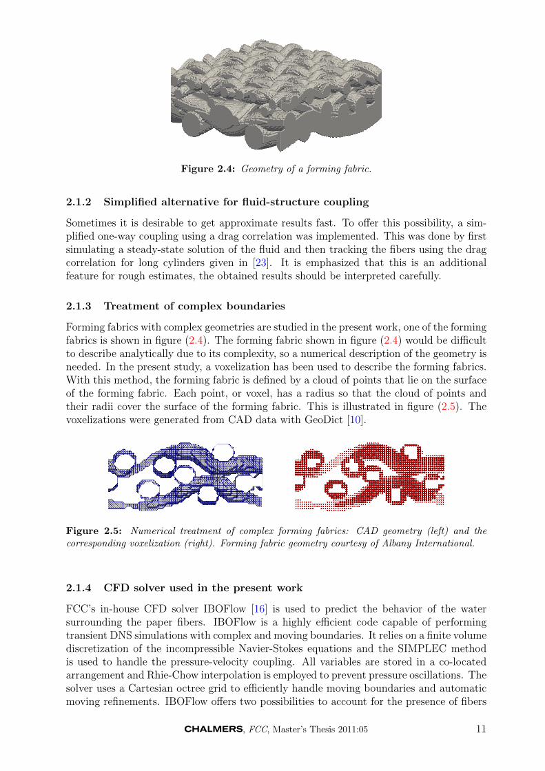
Figure 2.4: Geometry of a forming fabric.

2.1.2 Simplified alternative for fluid-structure coupling

Sometimes it is desirable to get approximate results fast. To offer this possibility, a sim-plified one-way coupling using a drag correlation was implemented. This was done by firstsimulating a steady-state solution of the fluid and then tracking the fibers using the dragcorrelation for long cylinders given in [23]. It is emphasized that this is an additionalfeature for rough estimates, the obtained results should be interpreted carefully.

2.1.3 Treatment of complex boundaries

Forming fabrics with complex geometries are studied in the present work, one of the formingfabrics is shown in figure (2.4). The forming fabric shown in figure (2.4) would be difficultto describe analytically due to its complexity, so a numerical description of the geometry isneeded. In the present study, a voxelization has been used to describe the forming fabrics.With this method, the forming fabric is defined by a cloud of points that lie on the surfaceof the forming fabric. Each point, or voxel, has a radius so that the cloud of points andtheir radii cover the surface of the forming fabric. This is illustrated in figure (2.5). Thevoxelizations were generated from CAD data with GeoDict [10].

Figure 2.5: Numerical treatment of complex forming fabrics: CAD geometry (left) and thecorresponding voxelization (right). Forming fabric geometry courtesy of Albany International.

2.1.4 CFD solver used in the present work

FCC’s in-house CFD solver IBOFlow [16] is used to predict the behavior of the watersurrounding the paper fibers. IBOFlow is a highly efficient code capable of performingtransient DNS simulations with complex and moving boundaries. It relies on a finite volumediscretization of the incompressible Navier-Stokes equations and the SIMPLEC methodis used to handle the pressure-velocity coupling. All variables are stored in a co-locatedarrangement and Rhie-Chow interpolation is employed to prevent pressure oscillations. Thesolver uses a Cartesian octree grid to efficiently handle moving boundaries and automaticmoving refinements. IBOFlow offers two possibilities to account for the presence of fibers


in the flow: the Mirroring Immersed Boundary method [21] and the Hybrid ImmersedBoundary method [22]. These methods are capable of fully resolving the flow around eachindividual fiber and constraining the fluid velocity to follow the fiber velocity with secondorder accuracy. The resolved velocity field allows computation of the fluid force acting ona fiber segment by integrating the traction vector over the surface of the fiber segment.

2.2 Fiber model

The Finite Element (FE) model of a fiber is built up in several steps. First, the geometry ofa fiber is described and definitions are introduced. Then the static FE model of a segmentwhich is only subjected to small rotations is formulated. This is a classical problem whichcan be found in many standard books on Finite Elements, see e.g. [15, 26]. However, herewe have the additional complication of a varying cross section. When the linear FE modelis established, the extensions necessary for finite rotations are described. This is achievedby using the method of co-rotational frames. Finally, inertia terms are added to the staticmodel so that transient simulations can be performed. Newmark’s interpolation is used tointerpolate velocities and accelerations in time. Hilber’s α-method [14] is used to introducenumerical dissipation without sacrificing the second order accuracy.

The ultimate goal of the discussion in this section is to obtain a tangent stiffness matrixand a residual force vector that can be used to perform a transient simulation with Newton’smethod. The internal force vector f

intand the inertia force vector f

mcan be computed as

described below. Fluid forces, contact forces and possibly gravity are added to the externalforce vector f

ext. When the solution has been found, the inertia force and internal force

should be balanced by the external force. Therefore, the residual is computed accordingto:

res = fext− f

int− f

m(2.7)

In the same way, the tangent stiffness matrix is composed of the Jacobian of the internalforce, the Jacobian of the inertia force and the Jacobian of the external forces:

K = Kint

+Km

+Kext

(2.8)

When the tangent stiffness matrix and the residual have been computed, these can be usedto take an iteration and find the increment ∆x:

∆x = −K−1 · res (2.9)

The increment vector ∆x contains the displacement increments ∆u and the rotation (spin)increments ∆ω. The nodal coordinates are updated with the displacement incrementsaccording to:

uk+1 = uk + ∆u (2.10)

The spin increment ∆ω is used to update the rotation matrix of the node as described later.When the displacements and rotations have been updated, the velocities and accelerationsare updated with Newmark’s method as described in [5].

2.2.1 Geometry of a fiber

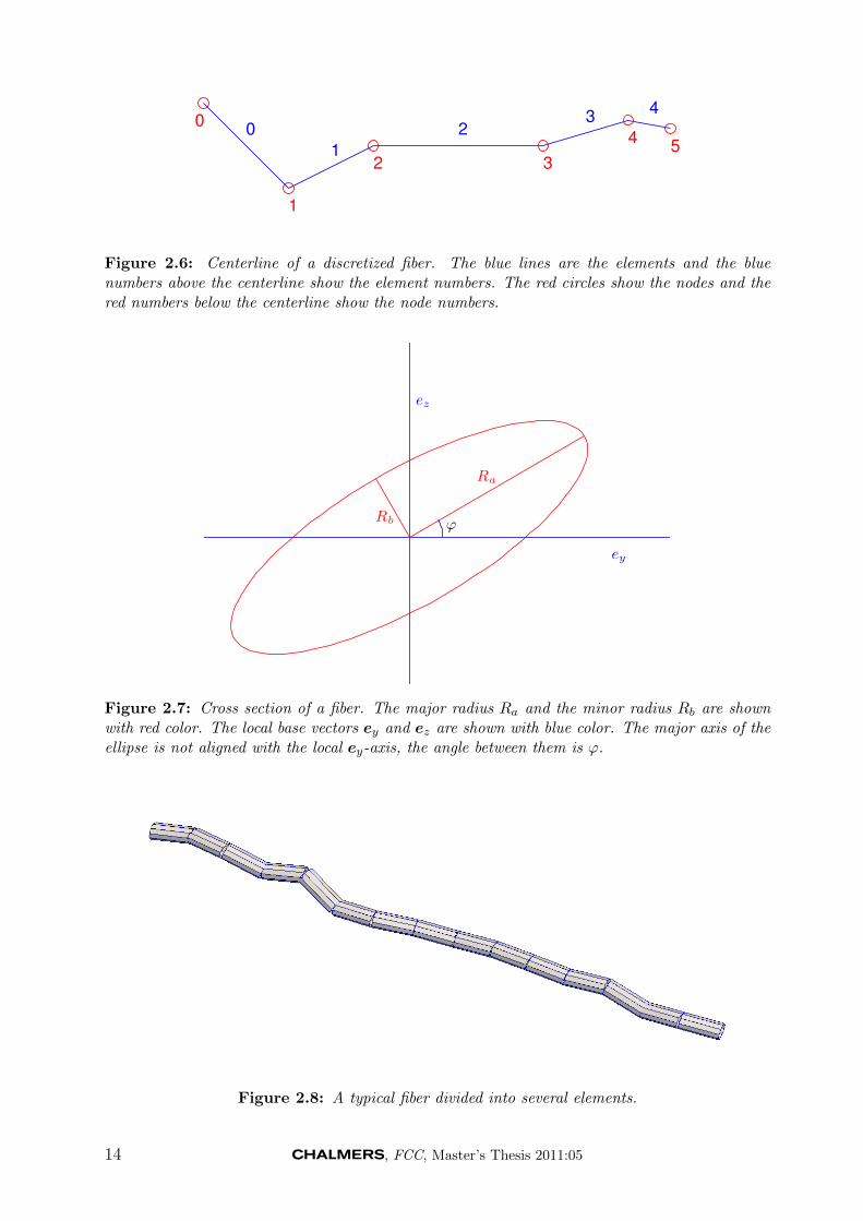
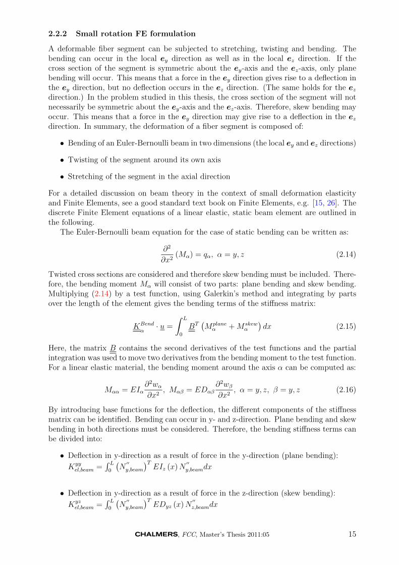
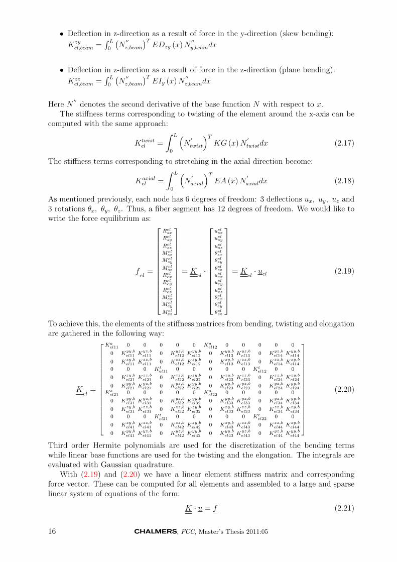
A fiber is discretized by dividing it into several elements. Each element is associated withtwo nodes, a node at the start point and a node at the end point. Figure (2.6) shows the


centerline of a fiber with nodes and elements highlighted. The fiber is assumed to have anelliptical cross section with major radius Ra and minor radius Rb. The cross section maybe hollow with interior major radius Ra,int and interior minor radius Rb,int. The majoraxis of the ellipse does not have to be aligned with the local ey-axis. The angle betweenthe major axis and the local ey-axis in the undeformed configuration is ϕ. A typical fibercross section with Ra, Rb and ϕ highlighted is shown in figure (2.7). The major radius Ra,the minor radius Rb and the angle ϕ are not constant, they may vary linearly along theaxis of the element.

Geometric nonlinearities will be accounted for in the present work and therefore a localcoordinate system is associated with every element. The base vectors of this local frameare defined as follows: The local ex vector lies along the line joining the start point and theend point of the element. If the start point is denoted by ps and the end point is denotedby pe, then ex is computed as:

ex =pe − ps|pe − ps|

(2.11)

The local ey-axis is aligned with the major axis in the start point when the element isundeformed. When the element is deformed, ey and ez are defined as proposed by Nour-Omid and Rankin [25]: Let q be a vector in the direction of the major axis in the startpoint. q is rigidly attached to the start point and rotates with the start point. ey and ezare computed from ex and q:

ez =ex × q|ex × q|

(2.12)

ey = ez × ex (2.13)

In this way, an orthogonal frame is constructed from the location of the nodes and thedirection of the major axis of the cross section.

Every node has 6 degrees of freedom: translation in 3 directions and rotation about 3axes. Hence a beam element has 12 degrees of freedom (dofs):

• 3 coordinates describing the location of the start point

• 3 angles describing rotation about the coordinate axes in the start point

• 3 coordinates describing the location of the end point

• 3 angles describing rotation about the coordinate axes in the end point

Figure (2.8) shows a typical fiber consisting of several elements.


0

1

2 3

45

0

1

23

4

Figure 2.6: Centerline of a discretized fiber. The blue lines are the elements and the bluenumbers above the centerline show the element numbers. The red circles show the nodes and thered numbers below the centerline show the node numbers.

Ra

Rb

ey

ez

ϕ

Figure 2.7: Cross section of a fiber. The major radius Ra and the minor radius Rb are shownwith red color. The local base vectors ey and ez are shown with blue color. The major axis of theellipse is not aligned with the local ey-axis, the angle between them is ϕ.

Figure 2.8: A typical fiber divided into several elements.


2.2.2 Small rotation FE formulation

A deformable fiber segment can be subjected to stretching, twisting and bending. Thebending can occur in the local ey direction as well as in the local ez direction. If thecross section of the segment is symmetric about the ey-axis and the ez-axis, only planebending will occur. This means that a force in the ey direction gives rise to a deflection inthe ey direction, but no deflection occurs in the ez direction. (The same holds for the ezdirection.) In the problem studied in this thesis, the cross section of the segment will notnecessarily be symmetric about the ey-axis and the ez-axis. Therefore, skew bending mayoccur. This means that a force in the ey direction may give rise to a deflection in the ezdirection. In summary, the deformation of a fiber segment is composed of:

• Bending of an Euler-Bernoulli beam in two dimensions (the local ey and ez directions)

• Twisting of the segment around its own axis

• Stretching of the segment in the axial direction

For a detailed discussion on beam theory in the context of small deformation elasticityand Finite Elements, see a good standard text book on Finite Elements, e.g. [15, 26]. Thediscrete Finite Element equations of a linear elastic, static beam element are outlined inthe following.

The Euler-Bernoulli beam equation for the case of static bending can be written as:

∂2

∂x2(Mα) = qα, α = y, z (2.14)

Twisted cross sections are considered and therefore skew bending must be included. There-fore, the bending moment Mα will consist of two parts: plane bending and skew bending.Multiplying (2.14) by a test function, using Galerkin’s method and integrating by partsover the length of the element gives the bending terms of the stiffness matrix:

KBend

α· u =

∫ L

0

BT(Mplane

α +M skewα

)dx (2.15)

Here, the matrix B contains the second derivatives of the test functions and the partialintegration was used to move two derivatives from the bending moment to the test function.For a linear elastic material, the bending moment around the axis α can be computed as:

Mαα = EIα∂2wα∂x2

, Mαβ = EDαβ∂2wβ∂x2

, α = y, z, β = y, z (2.16)

By introducing base functions for the deflection, the different components of the stiffnessmatrix can be identified. Bending can occur in y- and z-direction. Plane bending and skewbending in both directions must be considered. Therefore, the bending stiffness terms canbe divided into:

• Deflection in y-direction as a result of force in the y-direction (plane bending):

Kyyel,beam =

∫ L0

(N′′

y,beam

)TEIz (x)N

′′

y,beamdx

• Deflection in y-direction as a result of force in the z-direction (skew bending):

Kyzel,beam =

∫ L0

(N′′

y,beam

)TEDyz (x)N

′′

z,beamdx


• Deflection in z-direction as a result of force in the y-direction (skew bending):

Kzyel,beam =

∫ L0

(N′′

z,beam

)TEDzy (x)N

′′

y,beamdx

• Deflection in z-direction as a result of force in the z-direction (plane bending):

Kzzel,beam =

∫ L0

(N′′

z,beam

)TEIy (x)N

′′

z,beamdx

Here N′′

denotes the second derivative of the base function N with respect to x.The stiffness terms corresponding to twisting of the element around the x-axis can be

computed with the same approach:

Ktwistel =

∫ L

0

(N′

twist

)TKG (x)N

′

twistdx (2.17)

The stiffness terms corresponding to stretching in the axial direction become:

Kaxialel =

∫ L

0

(N′

axial

)TEA (x)N

′

axialdx (2.18)

As mentioned previously, each node has 6 degrees of freedom: 3 deflections ux, uy, uz and3 rotations θx, θy, θz. Thus, a fiber segment has 12 degrees of freedom. We would like towrite the force equilibrium as:

fel

=

RelsxRelsyRelszMelsx

Melsy

Melsz

RelexReleyRelezMelex

Meley

Melez

= K

el·

uelsxuelsyuelszθelsxθelsyθelszuelexueleyuelezθelexθeleyθelez

= K

el· uel (2.19)

To achieve this, the elements of the stiffness matrices from bending, twisting and elongationare gathered in the following way:

Kel

=

Kael11 0 0 0 0 0 Ka

el12 0 0 0 0 0

0 Kyy,bel11 Kyz,b

el11 0 Kyz,bel12 Kyy,b

el12 0 Kyy,bel13 Kyz,b


el14

0 Kzy,bel11 Kzz,b

el11 0 Kzz,bel12 Kzy,b

el12 0 Kzy,bel13 Kzz,b


el14

0 0 0 Ktel11 0 0 0 0 0 Kt

el12 0 0

0 Kzy,bel21 Kzz,b




el24

0 Kyy,bel21 Kyz,b




el24Kael21 0 0 0 0 0 Ka

el22 0 0 0 0 0

0 Kyy,bel31 Kyz,b




el34

0 Kzy,bel31 Kzz,b




el34

0 0 0 Ktel21 0 0 0 0 0 Kt

el22 0 0

0 Kzy,bel41 Kzz,b




el44

0 Kyy,bel41 Kyz,b




el44

(2.20)

Third order Hermite polynomials are used for the discretization of the bending termswhile linear base functions are used for the twisting and the elongation. The integrals areevaluated with Gaussian quadrature.

With (2.19) and (2.20) we have a linear element stiffness matrix and correspondingforce vector. These can be computed for all elements and assembled to a large and sparselinear system of equations of the form:

K · u = f (2.21)


This equation can be solved for u. For a discussion on the topic of assembling the elementmatrices to a global matrix, see e.g. [15].

2.2.3 Mathematics of finite rotations

In linear theory, angles are assumed to be small so that the local coordinate system ofeach element is constant. In the present work, angles can not be assumed to be small andtherefore the local element frame will not be constant. This fact necessitates the treatmentof rotating coordinate systems. Therefore, the elementary mathematics of finite rotationsis reviewed before proceeding with the formulation of nonlinear beam elements.

A coordinates system in space can be described with 3 base vectors: ex, ey and ez.These are the base vectors of the local frame, expressed in the global coordinate system.With these base vectors, a second order tensor E that transforms a vector from the localcoordinate system to the global coordinate system can be formed. This tensor has thelocal base vectors expressed in the global frame as columns:

E =[ex ey ez

](2.22)

A first order tensor v is transformed from local to global coordinates according to:

vglob = E · vloc (2.23)

A second order tensor A is transformed from local to global coordinates according to:

Aglob = E ·Aloc · ET (2.24)

As noted in [5], E is an orthogonal tensor and therefore has the following properties:

E−1 = ET ; det (E) = 1 (2.25)

An orthogonal second order tensor T can also represent a rotation. In such a case,there is a relation between the spin axis ω (a vector), the spin tensor Ω (a skew symmetrictensor) and the rotation tensor T (an orthogonal tensor). The relation between ω and Ωis defined by the spin operation S() [25]:

Ω = S (ω) = ω× =

0 −ω3 ω2

ω3 0 −ω1

−ω2 ω1 0

(2.26)

As noted in [25], S() is related to the cross product through (ω and r are vectors):

S (ω) · r = ω × r = −r × ω = −S (r) · ω (2.27)

The function axial() reverses the effect of spin:

axial (Ω) = axial

0 −ω3 ω2

ω3 0 −ω1

−ω2 ω1 0

=

ω1

ω2

ω3

= ω (2.28)

The relation between the spin tensor Ω and the corresponding rotation tensor T isgiven by the matrix exponent:

T = exp (Ω) (2.29)


The matrix logarithm reverses the effect of the matrix exponent:

Ω = log (T) (2.30)

Explicit expressions for the matrix exponential and the matrix logarithm are given inappendix A.

The above formulas can be used to update the rotations in the nodes. If a spin increment∆ω has been computed, the rotation matrix T can be updated according to [25]:

Tn+1 = exp (S (∆ω)) ·Tn (2.31)

Here n+1 denotes the new iteration step and n denotes the old iteration step. In equation(2.31), the rotation tensor is updated with a spin increment ∆ω. The linear FE formulationpresented in the previous section has the rotation angles as unknows. Therefore, it isnecessary to perform a change of variables from angles to spin variables. This can be doneby studying the variation of the angles at a node:

δθ =∂θ

∂ω· δω = Λ · δω (2.32)

The tensor Λ in the equation above was derived in [25]. An expression for Λ is given inappendix A.

2.2.4 Computation of element deformations

Measures of the deformation of an element are necessary to evaluate the internal forcevector. To identify the deformation of an element, consider a fiber segment subjected toan arbitrary motion expressed in the local coordinate system. The segment has 12 dofswith corresponding displacements and rotations:

uel = [ uels,x uels,y uels,z θels,x θels,y θels,zuele,x uele,y uele,z θele,x θele,y θele,z ] (2.33)

The local coordinate system is rigidly attached to the first node of the segment, so thedeformational displaclements in the first node are identically zero:

uels,x = uels,y = uels,z = 0 (2.34)

The ex-axis of the local coordinate system is always aligned with the centerline of thesegment. Therefore, the deformational displacement in the second node can be expressedas:

uele,x = l − L (2.35)

uele,y = uele,z = 0 (2.36)

Here, l is the length of the deformed segment and L is the initial length of the segment.In summary, the deformation of an element (with rigid body motion filtered out) in localcoordinates can be expressed as:

uel = [ 0 0 0 θels,x θels,y θ

els,z(l−L) 0 0 θele,x θ

ele,y θ

ele,z ] (2.37)

To calculate the length of a segment is trivial, but calculation of the deformational rotationsin (2.37) requires further attention. Let E denote the transformation matrix from the localframe to the global frame in the current configuration, as described in the previous section.Furthermore, let E0 denote the change of variables from the local frame to the global frame


in the initial configuration. Also, let T be a rotation matrix associated with each nodedescribing how a vector attached to that node has rotated. Then, the rotation matrixcorresponding to the rotational deformation can be computed according to equation (14)in [25]:

Te = ET ·Tg · E0 (2.38)

In equation (2.38), the notation used in [25] has been adopted, so that a superposed bardenotes the deformational part of a quatitiy. The superscript g denotes quantities expressedin global coordinates. It should be noted that the expression in (2.38) is not the only wayto compute the rotational deformation. See for example eqn (22) in [5] for an alternativeexpression. Eqn (2.38) gives a rotation matrix describing the rotational deformation. Thesmall deformation formulation requires the deformational rotation angles. Therefore, theseangles must be extracted from Te. This is done by using the matrix logarithm describedin the previous section:

θe = axial(log(Te)) (2.39)

2.2.5 Large rotation Finite Element formulation

This section presents the static terms in the nonlinear FE formulation used in the presentthesis. The co-rotational (CR) formulation proposed by Nour-Omid and Rankin [24],[25]is used. The essence of the co-rotational technique is that small strains are assumed,but the small strain finite element formulation is expressed in a coordinate system whichis attached to each element and moves with the element. In this way, the small strainformulation developed previously can be extended to include large rotation effects.

The linear formulation developed in the previous section is expressed with angles asrotational parameters. As noted previously, it is convenient to use spin variables to updatethe rotation tensors and therefore a change of variables must be performed. Following thework in [25], this change of variables transforms the small rotation internal force vectoraccording to:

fel

a

(uel,ωel

)= H

(θel

a

)· f

el

a

(uel,θ

el), a = s, e (2.40)

Here, H is given by:

H(θel

a

)=

I 0

0 Λ(θel

a

) =

I 0

0 ∂θela

∂ωela

, a = s, e (2.41)

Λ in equation (2.41) is given in appendix A. Now consider the internal force vector f ,

which in contrast to f and f properly accounts for finite rotations. f is the derivative ofthe strain energy Φ with respect to the nodal coordinates and rotations. Therefore, f canbe expressed as:

fi =∂φ

∂dj= Chain rule =

∂dj∂di

∂φ

∂dj= P T

ij f j (2.42)

Here di is a total displacement or a rotation in the node and di is the correspondingdeformational part of the displacement or rotation. The employment of the chain rule ineqn (2.42) reveals that the internal force vector can be written as a contraction of a matrixP and the linear, small deformation force vector f .

With the definition above, the matrix P is computed as:

Pij =∂di∂dj

(2.43)


Therefore, a 6 · 6 block of the matrix P , associated with nodes a and b is computed as:

Pab

=

∂uela∂uelb

∂uela∂ωelb

∂ωela∂uelb

∂ωela∂ωelb

; a = s, e; b = s, e (2.44)

In (2.44), ωela is the spin variable associated with node a, expressed in local coordinates.Transforming (2.42) to global coordinates gives the following expression for the internalforce vector:

f g = G · P T · f e (2.45)

Here G is the matrix that transforms a 12 · 1 vector from local to global coordinates:

G =

E 0 0 00 E 0 00 0 E 00 0 0 E

(2.46)

When the global equations of motion are solved, (2.45) enters the residual. To solvethe resulting system of equations with Newton’s method, the variation of (2.45) must becomputed. Following the work in [25], this is computed as:

δf g = G · P T · δf el +G · δP T · f el + δG · P T · f el (2.47)

The three terms in (2.47) are derived in [25]. Somewhat lengthy calculations give thefollowing expressions:

G · P T · δf el = G · P T ·Kel(uel,ωel

)· P ·GT · δdg

G · δP T · f el = (...) = −G · Γ · FT· P ·GT · δdg, F =

[S(felint,a)

0

]δG · P T · f el = (...) = −G · F · ΓT ·GT · δdg, F =

[S(felint,a)S(mel

int,a)

](2.48)

In (2.48), Γ is the derivative of the spin of the local element frame with respect to thenodal degrees of freedom. For a beam element with two nodes it is given by:

ΓT = [ ∂ωE∂us

∂ωE∂ωs

∂ωE∂ue

∂ωE∂ωe

] (2.49)

F and F in (2.48) are matrices which depend on the internal force vector, which has herebeen partitioned as:

f ela

=[felint,amelint,a

](2.50)

In the equation above, f elint,a is the internal element force associated with node a and melint,a

is the internal element moment associated with node a.An explicit epression for F is given in appendix B. Γ depends on the definition of

the local frame. An expression for Γ with the choice of coordinate system used in thepresent work is given in appendix B. Inserting the expressions in (2.48) into (2.47) givesthe following expression for the tangent stiffness matrix in local coordinates:

Kel = P T ·Kel · P − Γ · FT· P − F · ΓT (2.51)

It should be noted that the second and third terms in (2.51) are unsymmetric. For reasonsof computational efficiency, it is desirable to have a symmetric tangent stiffness matrix.


In [25] it is proven that the tangent stiffness in (2.51) can be symmetrized in such a waythat second order convergence of the Newton iterations is preserved. This symmetrizationtakes the following form:

Kel

symm= P T ·Kel · P − Γ · F T − P T · F · ΓT , F =

S(felint,s)S( 1

2melint,s)

S(felint,e)S( 1

2melint,e)

(2.52)

The matrix Kel

in (2.52) is the small deformation tangent stiffness expressed in spin vari-ables. Its 6 · 6 blocks associated with nodes a and b are given by:

Kel

ab

(uel,ωel

)= HT

a· K

el

ab

(uel,θ

el)·H

b+ δab

∂HT

a

∂ωelb· f el

a(2.53)

The equations (2.45) and (2.52) give expressions for the internal force vector and thecorresponding tangent stiffness, which can be used directly to solve quasi static problemssuch as the quasi static examples in the validation section. As noted in [25], the derivativeof H in (2.53) is negligible for a sufficiently fine grid.

2.2.6 Dynamic FE formulation

The equations (2.45) and (2.52) give the local internal force vector and tangent stiffness forthe quasistatic case. A simulation of paper fibers will be highly transient, especially whencollisions are present. Therefore, inertia effects must be added to the governing equations.The strong form of the equations of motion are given by equation (27) and (28) in [5]:

∂k

∂t= f ext +

∂

∂x(E · f int)

∂π

∂t= mext +

∂r

∂x× (E · f int) +

∂

∂x(E ·mint) (2.54)

Following the notation in [5], k is the linear momentum and π is the angular momentum.f ext is the externally applied body force and mext is the externally applied body moment.E is the transformation from local to global coordinates, f int is the internal force in apoint and mint is the internal moment in a point. Since this section deals with the inertiaterms, the expressions for ∂k

∂tand ∂π

∂tare considered. Equations (29) and (30) in [5] give

the follwing expressions for k and π for a beam cross section:

k = ρA∂u

∂t(2.55)

π = E · J · ET ·w (2.56)

Note that no assumptions on A and J have been introduced in (2.55) and (2.56), so thegeometry of the cross section may vary over the length of the segment. This is in contrastto the formulation in [5], where the cross section is assumed to be constant. In the presentwork, the geometry of the cross section will be allowed to vary throughout the derivationof the inertia terms.

First consider the linear momentum. Take the time derivative of (2.55) (where u isgiven in global coordinates):

∂k

∂t= ρA

∂2u

∂t2(2.57)


Now consider the angular momentum. Take the time derivative of (2.56):

·π =

·E · J · ET ·w + E · J ·

·ET ·w + E · J · ET · ·w =

= S (w) · E · J · ET ·w + E · J · (S (w) · E)T ·w + E · J · ET · ·w =

= S (w) · E · J · ET ·w + E · J · ET · ·w (2.58)

To get the weak form of the inertia force, multiply (2.58) by a test function N and integrateover the length of the beam element:

f gm

=

∫ l

0

N1

·k

N1·π

N2

·k

N2·π

dx =

∫ l

0

N1ρA

··u

N1

(S(w)·E·J·ET ·w+E·J·ET · ·w

)N2ρA

··u

N2

(S(w)·E·J·ET ·w+E·J·ET · ·w

)

dx (2.59)

Here N1 and N2 are the base functions. Galerkin’s method is used, so the functions used tointerpolate nodal quantities are the same as the test functions. Therefore, the quantitiesthat may vary with the axial coordinate are interpolated according to:

··u = N1

··u1 +N2

··u2

w = N1w1 +N2w2

·w = N1

·w1 +N2

·w2 (2.60)

Linear base functions are used to interpolate the inertia terms, as suggested in [5]. Theinformation given above is sufficient to evaluate the element inertia force numerically withGaussian quadrature. In order to solve the resulting system of equations with Newton’smethod, it is necessary to calculate the variation of (2.59). Taking this variation willrequire taking the variation of the local frame. In this thesis, the local frame is defined assuggested by Nour-Omid and Rankin [25]. This definition is different than the definitionof the element frame used in [5]. Therefore, the derivation of the Jacobian presented in[5] can not be used. A derivation of the Jacobian of the inertia force with the coordinatesystem used in the present work is given in appendix D.

2.3 Contact detection

Before any contact model can be applied, the fibers in contact must be identified. Moreprecisely, the point of contact and the overlap must be determined. For circular cylinderswith constant radius, an explicit formula for the contact point can easily be found. Forsegments with elliptic cross section with varying radii, the author has not succeeded tofind explicit formulas for the shortest distance between two segments. Therefore, theshortest distance and the corresponding collision normal must be computed iteratively.To iteratively locate contact points becomes computationally expensive and therefore it isnecessary to divide the contact detection into two step. First a search is performed basedonly on the nodal coordinates in order to find segments that are so close to each other thatthere is a possibility that contact might occur. Then the more expensive exact contactsearch is applied only to those segments that have been found to be so close to each otherthat contact could occur.

The section is divided into three parts. First, the algorithm used for locating segmentsthat are close each other is described. Then, an iterative scheme for finding the shortestdistance between a segment and a fixed, exterior point is derived. Finally, the shortestdistance between two segments is studied.


2.3.1 Spatial search - identifying segments that are close to each other

The problem of identifying collision candidates can be solved in different ways. The easiestway is to loop over all elements and check every element against all other elements. If thenumber of elements is N , the computational cost for this algorithm will scale like O (N2).For problems where N is large, the computational cost for contact detection with thisapproach becomes unacceptably high. As noted in [31], the computational time spent incontact search may be well over 80% of the total CPU time for a typical problem with 1000elements. Therefore an algorithm which scales better than O (N2) must be employed.

One good way to overcome this problem is to construct a binary search tree and usethe tree structure to search for contact pairs. The computational cost for creating a binarysearch tree is O (N log N) and the cost of searching is O (N log N) [32]. Therefore thetotal cost will also scale like O (N log N) which is much better than O (N2). In thepresent work, a kd-tree is used for the contact search. A kd-tree is a binary tree withnodes representing points in space. The points are inserted into the tree in such a waythat every node splits the space along one of the coordinate axes. Implementing a kd-treewas not a part of the present work, an implementation already available was used.

2.3.2 Distance between a segment and a fixed point

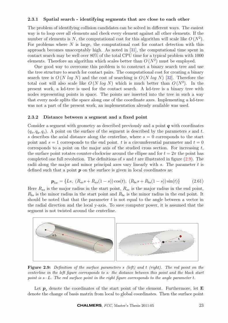
Consider a segment with geometry as described previously and a point q with coordinates(qx, qy, qz). A point on the surface of the segment is described by the parameters s and t.s describes the axial distance along the centerline, where s = 0 corresponds to the startpoint and s = 1 corresponds to the end point. t is a circumferential parameter and t = 0corresponds to a point on the major axis of the studied cross section. For increasing t,the surface point rotates counter-clockwise around the ellipse and for t = 2π the point hascompleted one full revolution. The definitions of s and t are illustrated in figure (2.9). Theradii along the major and minor principal axes vary linearly with s. The parameter t isdefined such that a point p on the surface is given in local coordinates as:

ploc = Ls, (Raes+Ras(1− s)) cos(t), (Rbes+Rbs(1− s)) sin(t) (2.61)

Here Ras is the major radius in the start point, Rae is the major radius in the end point,Rbs is the minor radius in the start point and Rbe is the minor radius in the end point. Itshould be noted that that the parameter t is not equal to the angle between a vector inthe radial direction and the local y-axis. To save computer power, it is assumed that thesegment is not twisted around the centerline.

Figure 2.9: Definition of the surface parameters s (left) and t (right). The red point on thecenterline in the left figure corresponds to s: the distance between this point and the black startpoint is s · L. The red surface point in the right figure corresponds to the angle parameter t.

Let ps denote the coordinates of the start point of the element. Furthermore, let Edenote the change of basis matrix from local to global coordinates. Then the surface point


can be expressed in global coordinates as:

p = ps + E · ploc (2.62)

Let the exterior point be q. Then a vector from the segment surface to the exteriorpoint can be calculated as:

d = q − p = q − ps − E · ploc (2.63)

The square of the distance between the surface and the exterior point is:

d2 = d · d (2.64)

The parameters (s, t) corresponding to the shortest distance between the segment surfaceand the exterior point can be found by solving the following minimization problem:

Find (s, t) such that d(s, t)→ min (2.65)

To find the parameters corresponding to the minimum of a distance which is always pos-itive, it is sufficient to find the minimum of the square of the distance. Therefore, theminimization problem in (2.65) can be reformulated as:

Find (s, t) such that (d(s, t))2 → min (2.66)

The function to be minimized in (2.66) has critical points when the gradient is zero:

∂

∂xα

(d2)

= 0, xα = (s, t) (2.67)

The equation in (2.67) can be solved with Newton’s method. To recast the problem intothe framework of Newton’s method in several variables, (2.67) is considered as a residualwhich should be forced to zero:

resα =∂

∂xα

(d2), xα = (s, t) (2.68)

Performing the differentiation in (2.68) gives the residual as:

res1 =∂d2

∂s= −2diEij

∂plocj∂s

res2 =∂d2

∂t= −2diEij

∂plocj∂t

(2.69)

To perform Newton iterations, the Jacobian K of the residual in (2.69) must be computed.The Jacobian is calculated as:

Kαβ =∂

∂xβ(resα) , xα = s, t, xβ = s, t (2.70)

Since the Jacobian of the residual is obtained by differentiating d2 twice, d2 can be consieredas a potential for the problem to be solved. Since the Jacobian of the residual (the Hessian


of d2) is derived from a potential, it will be symmetric. Performing the differentiation in(2.70) gives the following expressions for the Jacobian:

K11 =∂2d2

∂s∂s=

∂

∂s

(−2diEij

∂plocj∂s

)= 2Eik

∂plock∂s

Eij∂plocj∂s

K12 = K21 =∂2d2

∂t∂s=

∂

∂t

(−2diEij

∂plocj∂s

)= 2Eik

∂plock∂t

Eij∂plocj∂s− 2diEij

∂2plocj∂t∂s

K22 =∂2d2

∂t∂t=

∂

∂t

(−2diEij

∂plocj∂t

)= 2Eik

∂plock∂t

Eij∂plocj∂t− 2diEij

∂2plocj∂t∂t

(2.71)

The derivatives of the surface point coordinates in the local frame needed in (2.69) and(2.71) are:

∂ploc∂s

= [L, (Rae −Ras) cos(t), (Rbe −Rbs) sin(t)]

∂ploc∂t

= [0, sin(t)(−(Raes+Ras(1− s))), cos(t)(Rbes+RbS(1− s))]

∂2ploc∂s∂s

= [0, 0, 0]

∂2ploc∂t∂s

= [0, −(Rae −Ras) sin(t), (Rbe −Rbs) cos(t)]

∂2ploc∂t∂t

= [0, cos(t)(−(Raes+Ras(1− s))), sin(t)(−(Rbes+Rbs(1− s)))]

With expressions for the residual and the Jacobian available, Newton iterations can beperformed to get successively better approximations of the closest point on the segmentsurface. For each iteration, perform the following:

• ∆x = −K−1 · res

• x = x+ ∆x

• Terminate when converged

The procedure outlined above solves the unconstrained optimization problem of findingthe point on an elliptic surface which is closest to a given exterior point. It does notaccount for the constraint that the segment has finite length, so that the parameter s isconstrained: s ∈ [0, 1]. If s < 0, the closest point on the surface is on the edge at s = 0and if s > 1, the closest point is on the edge at s = 1. If this occurs, s should be set to 0or 1, depending on which edge has been encountered, and iterations should be performedto find the t corresponding to the shortest distance. To achieve this, the Jacobian derivedpreviously can be reduced so that the iterations do not change the value of s:

res1 = 0 (2.72)

K11 = 1 (2.73)

K12 = K21 = 0 (2.74)

By reducing the Jacobian in this way, the case where a point on the ellipse surface is closestto the exterior point and the case where a point on the edge is closest to the exterior pointcan be handled in the same iteration loop.


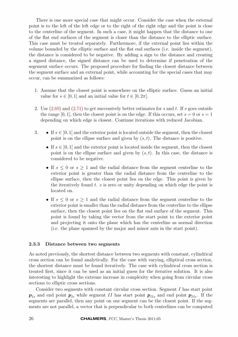
There is one more special case that might occur. Consider the case when the externalpoint is to the left of the left edge or to the right of the right edge and the point is closeto the centerline of the segment. In such a case, it might happen that the distance to oneof the flat end surfaces of the segment is closer than the distance to the elliptic surface.This case must be treated separately. Furthermore, if the external point lies within thevolume bounded by the elliptic surface and the flat end surfaces (i.e. inside the segment),the distance is considered to be negative. By adding a sign to the distance and creatinga signed distance, the signed distance can be used to determine if penetration of thesegement surface occurs. The proposed procedure for finding the closest distance betweenthe segment surface and an external point, while accounting for the special cases that mayoccur, can be summarized as follows:

1. Assume that the closest point is somewhere on the elliptic surface. Guess an initialvalue for s ∈ [0, 1] and an initial value for t ∈ [0, 2π].

2. Use (2.69) and (2.71) to get successively better estimates for s and t. If s goes outsidethe range [0, 1], then the closest point is on the edge. If this occurs, set s = 0 or s = 1depending on which edge is closest. Continue iterations with reduced Jacobian.

3. • If s ∈ ]0, 1[ and the exterior point is located outside the segment, then the closestpoint is on the ellipse surface and given by (s, t). The distance is positive.

• If s ∈ ]0, 1[ and the exterior point is located inside the segment, then the closestpoint is on the ellipse surface and given by (s, t). In this case, the distance isconsidered to be negative.

• If s ≤ 0 or s ≥ 1 and the radial distance from the segment centerline to theexterior point is greater than the radial distance from the centerline to theellipse surface, then the closest point lies on the edge. This point is given bythe iteratively found t. s is zero or unity depending on which edge the point islocated on.

• If s ≤ 0 or s ≥ 1 and the radial distance from the segment centerline to theexterior point is smaller than the radial distance from the centerline to the ellipsesurface, then the closest point lies on the flat end surface of the segment. Thispoint is found by taking the vector from the start point to the exterior pointand projecting it onto the plane which has the centerline as normal direction(i.e. the plane spanned by the major and minor axis in the start point).

2.3.3 Distance between two segments

As noted previously, the shortest distance between two segments with constant, cylindricalcross section can be found analytically. For the case with varying, elliptical cross section,the shortest distance must be found iteratively. The case with cylindrical cross section istreated first, since it can be used as an initial guess for the iterative solution. It is alsointeresting to highlight the extreme increase in complexity when going from circular crosssections to elliptic cross sections.

Consider two segments with constant circular cross section. Segment I has start pointpIs and end point pIe while segment II has start point pIIs and end point pIIe. If thesegments are parallel, then any point on one segment can be the closest point. If the seg-ments are not parallel, a vector that is perpendicular to both centerlines can be computed


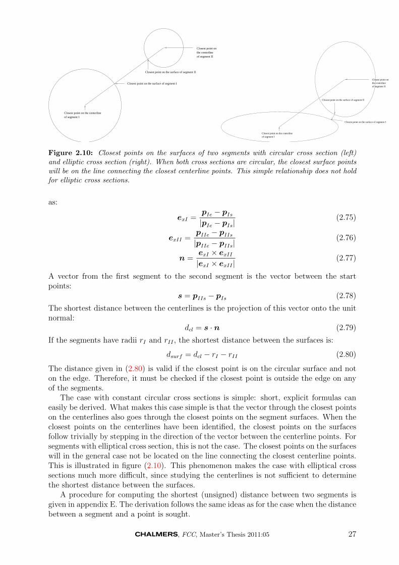
Closest point on the centerlineof segment I

Closest point on the surface of segment I

Closest point on the surface of segment II

Closest point onthe centerlineof segment II

Closest point on the centerlineof segment I

Closest point onthe centerlineof segment II

Closest point on the surface of segment II

Closest point on the surface of segment I

Figure 2.10: Closest points on the surfaces of two segments with circular cross section (left)and elliptic cross section (right). When both cross sections are circular, the closest surface pointswill be on the line connecting the closest centerline points. This simple relationship does not holdfor elliptic cross sections.

as:

exI =pIe − pIs|pIe − pIs|

(2.75)

exII =pIIe − pIIs|pIIe − pIIs|

(2.76)

n =exI × exII|exI × exII |

(2.77)

A vector from the first segment to the second segment is the vector between the startpoints:

s = pIIs − pIs (2.78)

The shortest distance between the centerlines is the projection of this vector onto the unitnormal:

dcl = s · n (2.79)

If the segments have radii rI and rII , the shortest distance between the surfaces is:

dsurf = dcl − rI − rII (2.80)

The distance given in (2.80) is valid if the closest point is on the circular surface and noton the edge. Therefore, it must be checked if the closest point is outside the edge on anyof the segments.

The case with constant circular cross sections is simple: short, explicit formulas caneasily be derived. What makes this case simple is that the vector through the closest pointson the centerlines also goes through the closest points on the segment surfaces. When theclosest points on the centerlines have been identified, the closest points on the surfacesfollow trivially by stepping in the direction of the vector between the centerline points. Forsegments with elliptical cross section, this is not the case. The closest points on the surfaceswill in the general case not be located on the line connecting the closest centerline points.This is illustrated in figure (2.10). This phenomenon makes the case with elliptical crosssections much more difficult, since studying the centerlines is not sufficient to determinethe shortest distance between the surfaces.

A procedure for computing the shortest (unsigned) distance between two segments isgiven in appendix E. The derivation follows the same ideas as for the case when the distancebetween a segment and a point is sought.


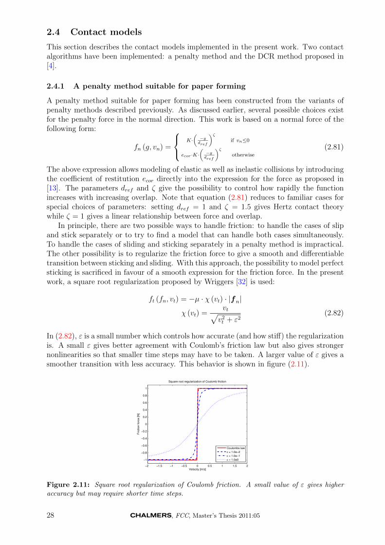
2.4 Contact models

This section describes the contact models implemented in the present work. Two contactalgorithms have been implemented: a penalty method and the DCR method proposed in[4].

2.4.1 A penalty method suitable for paper forming

A penalty method suitable for paper forming has been constructed from the variants ofpenalty methods described previously. As discussed earlier, several possible choices existfor the penalty force in the normal direction. This work is based on a normal force of thefollowing form:

fn (g, vn) =

K·(−gdref

)ζif vn≤0

ecor·K·(−gdref

)ζotherwise

(2.81)

The above expression allows modeling of elastic as well as inelastic collisions by introducingthe coefficient of restitution ecor directly into the expression for the force as proposed in[13]. The parameters dref and ζ give the possibility to control how rapidly the functionincreases with increasing overlap. Note that equation (2.81) reduces to familiar cases forspecial choices of parameters: setting dref = 1 and ζ = 1.5 gives Hertz contact theorywhile ζ = 1 gives a linear relationship between force and overlap.

In principle, there are two possible ways to handle friction: to handle the cases of slipand stick separately or to try to find a model that can handle both cases simultaneously.To handle the cases of sliding and sticking separately in a penalty method is impractical.The other possibility is to regularize the friction force to give a smooth and differentiabletransition between sticking and sliding. With this approach, the possibility to model perfectsticking is sacrificed in favour of a smooth expression for the friction force. In the presentwork, a square root regularization proposed by Wriggers [32] is used:

ft (fn, vt) = −µ · χ (vt) · |fn|

χ (vt) =vt√v2t + ε2

(2.82)

In (2.82), ε is a small number which controls how accurate (and how stiff) the regularizationis. A small ε gives better agreement with Coulomb’s friction law but also gives strongernonlinearities so that smaller time steps may have to be taken. A larger value of ε gives asmoother transition with less accuracy. This behavior is shown in figure (2.11).

−2 −1.5 −1 −0.5 0 0.5 1 1.5 2

−1

−0.8

−0.6

−0.4

−0.2

0

0.2

0.4

0.6

0.8

1

Velocity [m/s]

Friction forc

e [N

]

Square root regularization of Coulomb friction

Coulombs law

ε = 1.0e−2

ε = 1.0e−1

ε = 1.0e0

Figure 2.11: Square root regularization of Coulomb friction. A small value of ε gives higheraccuracy but may require shorter time steps.


When the magnitude of the normal force and the tangential force have been computed,the total contact force is computed as:

f = fnn+ ftt (2.83)

Here n is the contact normal direction and t is the tangential sliding direction. n iscomputed as (pI and pII are the closest points on segment I and II):

n =pII − pI|pII − pI |

if |pII − pI | 6= 0 (2.84)

n =∂pI∂s× ∂pI

∂t∣∣∣∂pI∂s × ∂pI∂t

∣∣∣ otherwise (2.85)

i.e. the normal is taken as the closest point on surface II minus the closest point on surfaceI if these points do not coincide. If the closest points do coincide, the collision normal isinstead taken as the normal direction of surface I.

The tangential sliding direction is computed as:

t =vtang|vtang|

if |vtang| 6= 0 (2.86)

t = 0 otherwise (2.87)

Note that t could be set to any value if |vtang| = 0, because in this case the friction forcewill be zero any way.

The contact force is a function of the overlap and the relative velocity, which in turnare functions of the nodal positions at the current time step. As a result, the contact forceswill change during the iterations of a single time step. Therefore, only adding the contactforces to the right hand side without changing the tangent stiffness matrix will destroythe second order convergence of the Newton iterations. In order to retain second orderconvergence, the Jacobian of the contact must be computed and added to the tangentstiffness matrix. As mentioned previously, the author has not succeeded to find an explicitexpression for the contact point. Therefore it is not possible to compute the Jacobian ofthe contact force analytically and two options remain:

• Compute the Jacobian of the contact force numerically. This is always possible, butit comes at an increased computational cost.

• Perform the simulation without using a Jacobian for the contact force and acceptthat the convergence will not be second order.

Both options have been tried in the present work. It was found that the loss of convergencewas small for the cases of interest here and therefore most of the simulations were performedwithout using a Jacobian for the contact force.

2.4.2 Decomposition Contact Response

The algorithm proposed by Cirak and West [4] has been implemented in the present work.Next, the algorithm given in [4] is described in greater detail than in the introduction.Then, modifications are proposed to make the algorithm suitable for simulations of paperforming.

The DCR method is an algorithm of predictor-corrector type: first a predictor time stepis taken as if no contacts occured, then interpenetrations are removed and velocities are


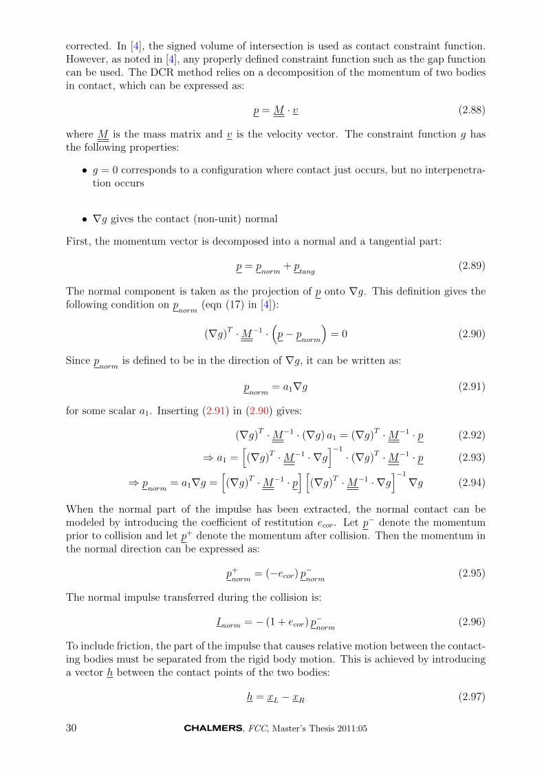
corrected. In [4], the signed volume of intersection is used as contact constraint function.However, as noted in [4], any properly defined constraint function such as the gap functioncan be used. The DCR method relies on a decomposition of the momentum of two bodiesin contact, which can be expressed as:

p = M · v (2.88)

where M is the mass matrix and v is the velocity vector. The constraint function g hasthe following properties:

• g = 0 corresponds to a configuration where contact just occurs, but no interpenetra-tion occurs

• ∇g gives the contact (non-unit) normal

First, the momentum vector is decomposed into a normal and a tangential part:

p = pnorm

+ ptang

(2.89)

The normal component is taken as the projection of p onto ∇g. This definition gives thefollowing condition on p

norm(eqn (17) in [4]):

(∇g)T ·M−1 ·(p− p

norm

)= 0 (2.90)

Since pnorm

is defined to be in the direction of ∇g, it can be written as:

pnorm

= a1∇g (2.91)

for some scalar a1. Inserting (2.91) in (2.90) gives:

(∇g)T ·M−1 · (∇g) a1 = (∇g)T ·M−1 · p (2.92)

⇒ a1 =[(∇g)T ·M−1 · ∇g

]−1

· (∇g)T ·M−1 · p (2.93)

⇒ pnorm

= a1∇g =[(∇g)T ·M−1 · p

] [(∇g)T ·M−1 · ∇g

]−1

∇g (2.94)

When the normal part of the impulse has been extracted, the normal contact can bemodeled by introducing the coefficient of restitution ecor. Let p− denote the momentumprior to collision and let p+ denote the momentum after collision. Then the momentum inthe normal direction can be expressed as:

p+

norm= (−ecor) p−norm (2.95)

The normal impulse transferred during the collision is:

Inorm = − (1 + ecor) p−norm

(2.96)

To include friction, the part of the impulse that causes relative motion between the contact-ing bodies must be separated from the rigid body motion. This is achieved by introducinga vector h between the contact points of the two bodies:

h = xL − xR (2.97)


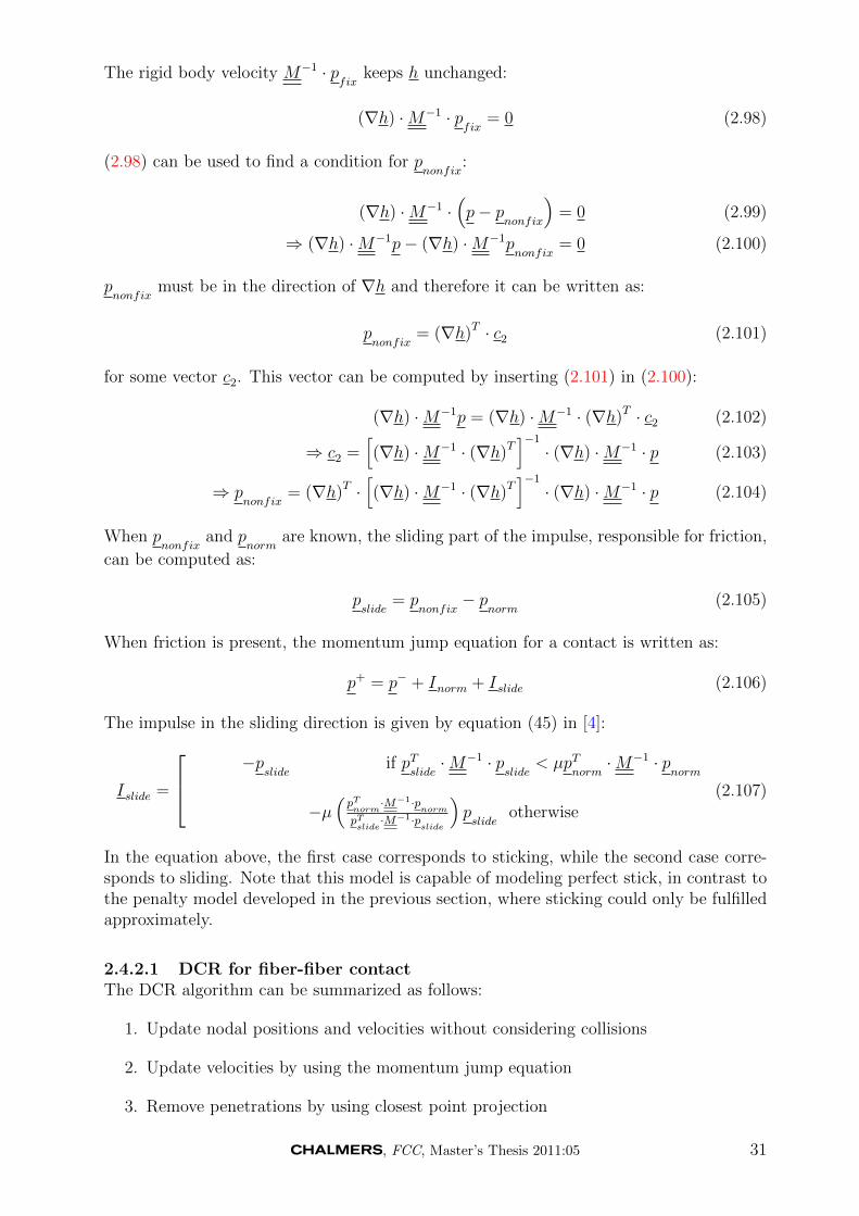
The rigid body velocity M−1 · pfix

keeps h unchanged:

(∇h) ·M−1 · pfix

= 0 (2.98)

(2.98) can be used to find a condition for pnonfix

:

(∇h) ·M−1 ·(p− p

nonfix

)= 0 (2.99)

⇒ (∇h) ·M−1p− (∇h) ·M−1pnonfix

= 0 (2.100)

pnonfix

must be in the direction of ∇h and therefore it can be written as:

pnonfix

= (∇h)T · c2 (2.101)

for some vector c2. This vector can be computed by inserting (2.101) in (2.100):

(∇h) ·M−1p = (∇h) ·M−1 · (∇h)T · c2 (2.102)

⇒ c2 =[(∇h) ·M−1 · (∇h)T

]−1

· (∇h) ·M−1 · p (2.103)

⇒ pnonfix

= (∇h)T ·[(∇h) ·M−1 · (∇h)T

]−1

· (∇h) ·M−1 · p (2.104)

When pnonfix

and pnorm

are known, the sliding part of the impulse, responsible for friction,

can be computed as:

pslide

= pnonfix

− pnorm

(2.105)

When friction is present, the momentum jump equation for a contact is written as:

p+ = p− + Inorm + Islide (2.106)

The impulse in the sliding direction is given by equation (45) in [4]:

Islide =

−pslide

if pTslide·M−1 · p

slide< µpT

norm·M−1 · p

norm

−µ(pTnorm

·M−1·pnorm

pTslide·M−1·p

slide

)pslide

otherwise(2.107)

In the equation above, the first case corresponds to sticking, while the second case corre-sponds to sliding. Note that this model is capable of modeling perfect stick, in contrast tothe penalty model developed in the previous section, where sticking could only be fulfilledapproximately.

2.4.2.1 DCR for fiber-fiber contactThe DCR algorithm can be summarized as follows:

1. Update nodal positions and velocities without considering collisions

2. Update velocities by using the momentum jump equation

3. Remove penetrations by using closest point projection


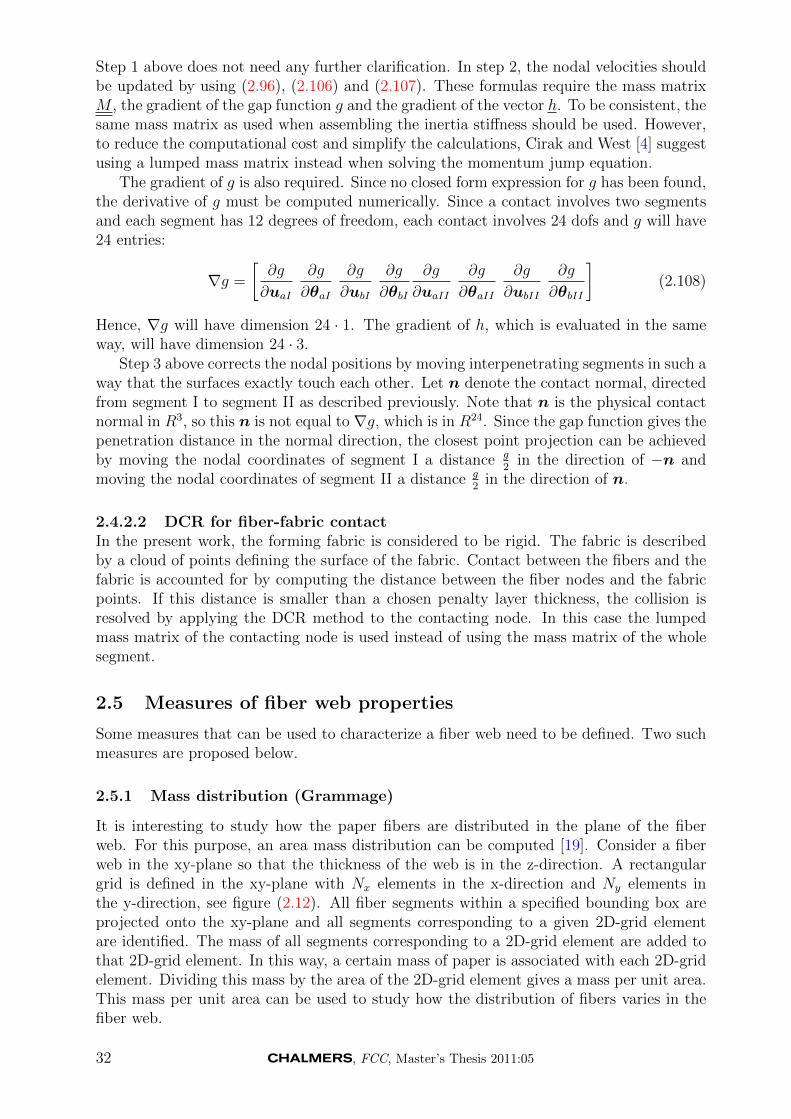
Step 1 above does not need any further clarification. In step 2, the nodal velocities shouldbe updated by using (2.96), (2.106) and (2.107). These formulas require the mass matrixM , the gradient of the gap function g and the gradient of the vector h. To be consistent, thesame mass matrix as used when assembling the inertia stiffness should be used. However,to reduce the computational cost and simplify the calculations, Cirak and West [4] suggestusing a lumped mass matrix instead when solving the momentum jump equation.

The gradient of g is also required. Since no closed form expression for g has been found,the derivative of g must be computed numerically. Since a contact involves two segmentsand each segment has 12 degrees of freedom, each contact involves 24 dofs and g will have24 entries:

∇g =

[∂g

∂uaI

∂g

∂θaI

∂g

∂ubI

∂g

∂θbI

∂g

∂uaII

∂g

∂θaII

∂g

∂ubII

∂g

∂θbII

](2.108)

Hence, ∇g will have dimension 24 · 1. The gradient of h, which is evaluated in the sameway, will have dimension 24 · 3.

Step 3 above corrects the nodal positions by moving interpenetrating segments in such away that the surfaces exactly touch each other. Let n denote the contact normal, directedfrom segment I to segment II as described previously. Note that n is the physical contactnormal in R3, so this n is not equal to ∇g, which is in R24. Since the gap function gives thepenetration distance in the normal direction, the closest point projection can be achievedby moving the nodal coordinates of segment I a distance g

2in the direction of −n and

moving the nodal coordinates of segment II a distance g2

in the direction of n.

2.4.2.2 DCR for fiber-fabric contactIn the present work, the forming fabric is considered to be rigid. The fabric is describedby a cloud of points defining the surface of the fabric. Contact between the fibers and thefabric is accounted for by computing the distance between the fiber nodes and the fabricpoints. If this distance is smaller than a chosen penalty layer thickness, the collision isresolved by applying the DCR method to the contacting node. In this case the lumpedmass matrix of the contacting node is used instead of using the mass matrix of the wholesegment.

2.5 Measures of fiber web properties

Some measures that can be used to characterize a fiber web need to be defined. Two suchmeasures are proposed below.

2.5.1 Mass distribution (Grammage)

It is interesting to study how the paper fibers are distributed in the plane of the fiberweb. For this purpose, an area mass distribution can be computed [19]. Consider a fiberweb in the xy-plane so that the thickness of the web is in the z-direction. A rectangulargrid is defined in the xy-plane with Nx elements in the x-direction and Ny elements inthe y-direction, see figure (2.12). All fiber segments within a specified bounding box areprojected onto the xy-plane and all segments corresponding to a given 2D-grid elementare identified. The mass of all segments corresponding to a 2D-grid element are added tothat 2D-grid element. In this way, a certain mass of paper is associated with each 2D-gridelement. Dividing this mass by the area of the 2D-grid element gives a mass per unit area.This mass per unit area can be used to study how the distribution of fibers varies in thefiber web.


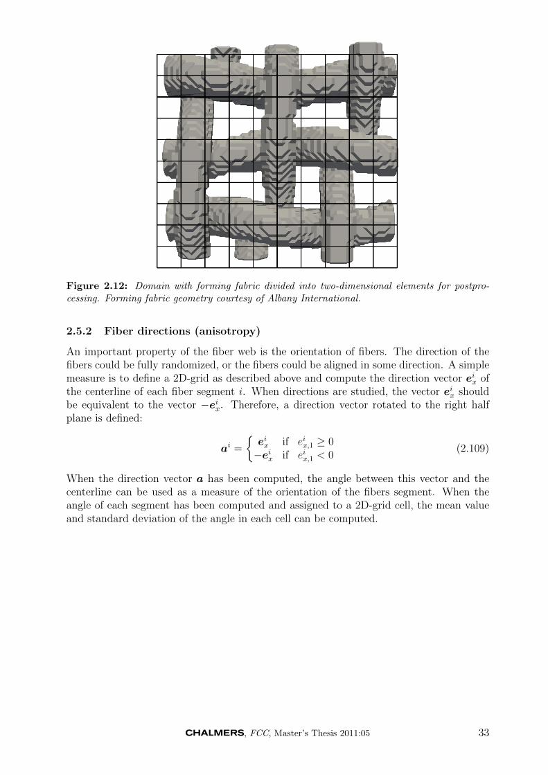
Figure 2.12: Domain with forming fabric divided into two-dimensional elements for postpro-cessing. Forming fabric geometry courtesy of Albany International.

2.5.2 Fiber directions (anisotropy)

An important property of the fiber web is the orientation of fibers. The direction of thefibers could be fully randomized, or the fibers could be aligned in some direction. A simplemeasure is to define a 2D-grid as described above and compute the direction vector eix ofthe centerline of each fiber segment i. When directions are studied, the vector eix shouldbe equivalent to the vector −eix. Therefore, a direction vector rotated to the right halfplane is defined:

ai =

eix if eix,1 ≥ 0−eix if eix,1 < 0

(2.109)

When the direction vector a has been computed, the angle between this vector and thecenterline can be used as a measure of the orientation of the fibers segment. When theangle of each segment has been computed and assigned to a 2D-grid cell, the mean valueand standard deviation of the angle in each cell can be computed.


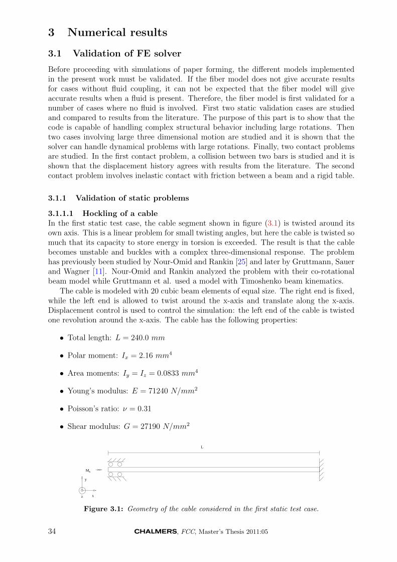
3 Numerical results

3.1 Validation of FE solver

Before proceeding with simulations of paper forming, the different models implementedin the present work must be validated. If the fiber model does not give accurate resultsfor cases without fluid coupling, it can not be expected that the fiber model will giveaccurate results when a fluid is present. Therefore, the fiber model is first validated for anumber of cases where no fluid is involved. First two static validation cases are studiedand compared to results from the literature. The purpose of this part is to show that thecode is capable of handling complex structural behavior including large rotations. Thentwo cases involving large three dimensional motion are studied and it is shown that thesolver can handle dynamical problems with large rotations. Finally, two contact problemsare studied. In the first contact problem, a collision between two bars is studied and it isshown that the displacement history agrees with results from the literature. The secondcontact problem involves inelastic contact with friction between a beam and a rigid table.

3.1.1 Validation of static problems

3.1.1.1 Hockling of a cableIn the first static test case, the cable segment shown in figure (3.1) is twisted around itsown axis. This is a linear problem for small twisting angles, but here the cable is twisted somuch that its capacity to store energy in torsion is exceeded. The result is that the cablebecomes unstable and buckles with a complex three-dimensional response. The problemhas previously been studied by Nour-Omid and Rankin [25] and later by Gruttmann, Sauerand Wagner [11]. Nour-Omid and Rankin analyzed the problem with their co-rotationalbeam model while Gruttmann et al. used a model with Timoshenko beam kinematics.

The cable is modeled with 20 cubic beam elements of equal size. The right end is fixed,while the left end is allowed to twist around the x-axis and translate along the x-axis.Displacement control is used to control the simulation: the left end of the cable is twistedone revolution around the x-axis. The cable has the following properties:

• Total length: L = 240.0 mm

• Polar moment: Ix = 2.16 mm4

• Area moments: Iy = Iz = 0.0833 mm4

• Young’s modulus: E = 71240 N/mm2

• Poisson’s ratio: ν = 0.31

• Shear modulus: G = 27190 N/mm2

Mx

L

x

y

z

Figure 3.1: Geometry of the cable considered in the first static test case.


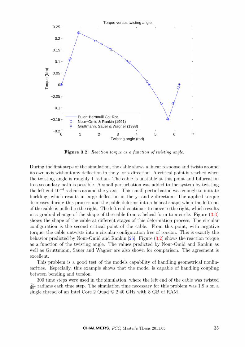
0 1 2 3 4 5 6 7−0.2

−0.15

−0.1

−0.05

0

0.05

0.1

0.15

0.2

0.25Torque versus twisting angle

Twisting angle (rad)

Tor

que

(Nm

)

Euler−Bernoulli Co−Rot.Nour−Omid & Rankin (1991)Gruttmann, Sauer & Wagner (1998)

Figure 3.2: Reaction torque as a function of twisting angle.

During the first steps of the simulation, the cable shows a linear response and twists aroundits own axis without any deflection in the y- or z-direction. A critical point is reached whenthe twisting angle is roughly 1 radian. The cable is unstable at this point and bifurcationto a secondary path is possible. A small perturbation was added to the system by twistingthe left end 10−4 radians around the y-axis. This small perturbation was enough to initiatebuckling, which results in large deflection in the y- and z-direction. The applied torquedecreases during this process and the cable deforms into a helical shape when the left endof the cable is pulled to the right. The left end continues to move to the right, which resultsin a gradual change of the shape of the cable from a helical form to a circle. Figure (3.3)shows the shape of the cable at different stages of this deformation process. The circularconfiguration is the second critical point of the cable. From this point, with negativetorque, the cable untwists into a circular configuration free of torsion. This is exactly thebehavior predicted by Nour-Omid and Rankin [25]. Figure (3.2) shows the reaction torqueas a function of the twisting angle. The values predicted by Nour-Omid and Rankin aswell as Gruttmann, Sauer and Wagner are also shown for comparison. The agreement isexcellent.

This problem is a good test of the models capability of handling geometrical nonlin-earities. Especially, this example shows that the model is capable of handling couplingbetween bending and torsion.

300 time steps were used in the simulation, where the left end of the cable was twisted2π300

radians each time step. The simulation time necessary for this problem was 1.9 s on asingle thread of an Intel Core 2 Quad @ 2.40 GHz with 8 GB of RAM.


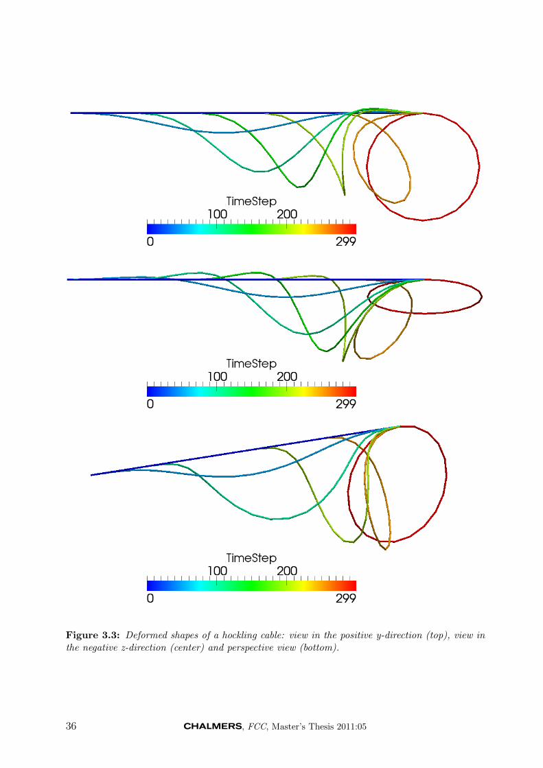
Figure 3.3: Deformed shapes of a hockling cable: view in the positive y-direction (top), view inthe negative z-direction (center) and perspective view (bottom).


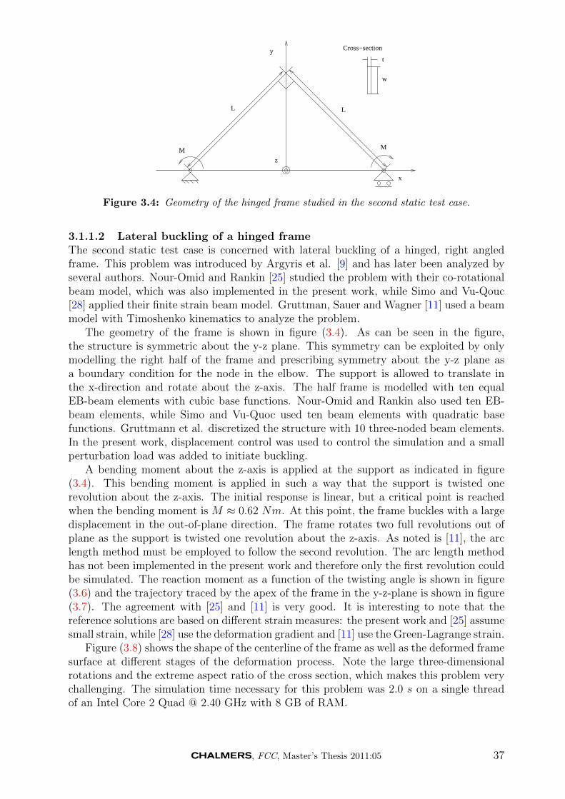
x

y

LL

Cross−section

t

w

M M

z

Figure 3.4: Geometry of the hinged frame studied in the second static test case.

3.1.1.2 Lateral buckling of a hinged frameThe second static test case is concerned with lateral buckling of a hinged, right angledframe. This problem was introduced by Argyris et al. [9] and has later been analyzed byseveral authors. Nour-Omid and Rankin [25] studied the problem with their co-rotationalbeam model, which was also implemented in the present work, while Simo and Vu-Qouc[28] applied their finite strain beam model. Gruttman, Sauer and Wagner [11] used a beammodel with Timoshenko kinematics to analyze the problem.

The geometry of the frame is shown in figure (3.4). As can be seen in the figure,the structure is symmetric about the y-z plane. This symmetry can be exploited by onlymodelling the right half of the frame and prescribing symmetry about the y-z plane asa boundary condition for the node in the elbow. The support is allowed to translate inthe x-direction and rotate about the z-axis. The half frame is modelled with ten equalEB-beam elements with cubic base functions. Nour-Omid and Rankin also used ten EB-beam elements, while Simo and Vu-Quoc used ten beam elements with quadratic basefunctions. Gruttmann et al. discretized the structure with 10 three-noded beam elements.In the present work, displacement control was used to control the simulation and a smallperturbation load was added to initiate buckling.

A bending moment about the z-axis is applied at the support as indicated in figure(3.4). This bending moment is applied in such a way that the support is twisted onerevolution about the z-axis. The initial response is linear, but a critical point is reachedwhen the bending moment is M ≈ 0.62 Nm. At this point, the frame buckles with a largedisplacement in the out-of-plane direction. The frame rotates two full revolutions out ofplane as the support is twisted one revolution about the z-axis. As noted is [11], the arclength method must be employed to follow the second revolution. The arc length methodhas not been implemented in the present work and therefore only the first revolution couldbe simulated. The reaction moment as a function of the twisting angle is shown in figure(3.6) and the trajectory traced by the apex of the frame in the y-z-plane is shown in figure(3.7). The agreement with [25] and [11] is very good. It is interesting to note that thereference solutions are based on different strain measures: the present work and [25] assumesmall strain, while [28] use the deformation gradient and [11] use the Green-Lagrange strain.

Figure (3.8) shows the shape of the centerline of the frame as well as the deformed framesurface at different stages of the deformation process. Note the large three-dimensionalrotations and the extreme aspect ratio of the cross section, which makes this problem verychallenging. The simulation time necessary for this problem was 2.0 s on a single threadof an Intel Core 2 Quad @ 2.40 GHz with 8 GB of RAM.


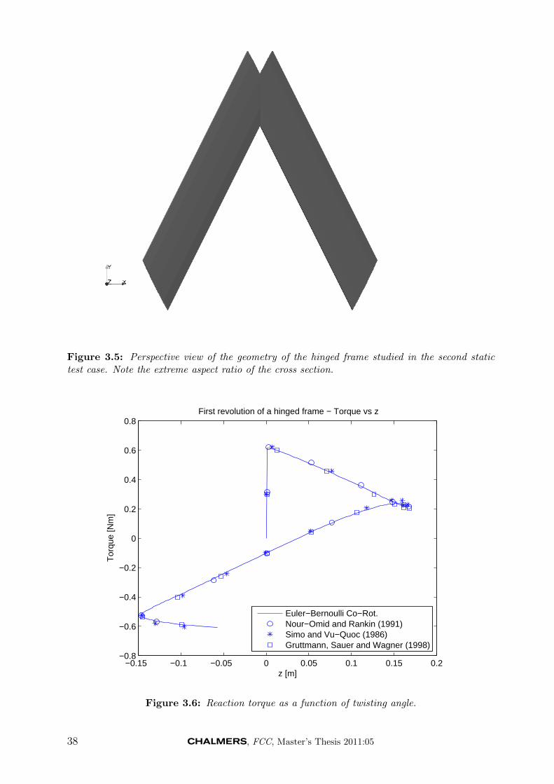
Figure 3.5: Perspective view of the geometry of the hinged frame studied in the second statictest case. Note the extreme aspect ratio of the cross section.

−0.15 −0.1 −0.05 0 0.05 0.1 0.15 0.2−0.8

−0.6

−0.4

−0.2

0

0.2

0.4

0.6

0.8First revolution of a hinged frame − Torque vs z

z [m]

Tor

que

[Nm

]

Euler−Bernoulli Co−Rot.Nour−Omid and Rankin (1991)Simo and Vu−Quoc (1986)Gruttmann, Sauer and Wagner (1998)

Figure 3.6: Reaction torque as a function of twisting angle.


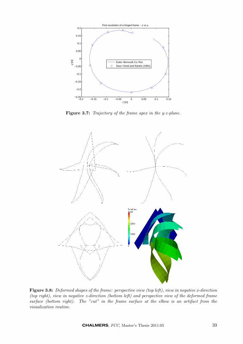
−0.2 −0.15 −0.1 −0.05 0 0.05 0.1 0.15−0.25

−0.2

−0.15

−0.1

−0.05

0

0.05

0.1

0.15

0.2First revolution of a hinged frame − z vs y

z [m]

y [m

]

Euler−Bernoulli Co−Rot.

Nour−Omid and Rankin (1991)

Figure 3.7: Trajectory of the frame apex in the y-z-plane.

Figure 3.8: Deformed shapes of the frame: perspective view (top left), view in negative x-direction(top right), view in negative z-direction (bottom left) and perspective view of the deformed framesurface (bottom right). The ”cut” in the frame surface at the elbow is an artifact from thevisualization routine.


3.1.2 Validation of dynamic problems

3.1.2.1 Free vibration of right-angle cantilever beamThe first dynamic test case hase been studied by several authors, among others Simo andVu-Quoc [29] and later Ibrahimbegovic and Mikdad [17]. In this problem, the L-shapedcantilever beam shown in figure (3.9) is studied. A point force is applied in the out-of-plane direction at the elbow. Figure (3.9) shows the time history of the force, which hasa maximum value of 50 N and is applied for two seconds. The geometry of the beam isdefined in figure (3.9) and the properties of the cross section are:

• GAy = GAz = EA = 106

• EIy = EIz = GJ = 103

• Aρ = 1

• Iρx = 20

• Iρy = Iρz = 10

It should be noted that in the present work, a model based on the Euler-Bernoulli beamtheory was used, which implicitly assumes GAy = GAz = ∞. As will be seen, thisassumption does not have a noticeable effect on the results for this test case. The reasonfor this is most likely that the structure studied in this problem is indeed very slender andtherefore the Euler-Bernoulli assumption is justified.

The beam is initially at rest and starts to deflect when the external force is applied.After the force has been removed, the structure performs free vibrations with large magni-tude. As noted in [17], the amplitude of the vibration is of the same order of magnitude asthe length of the structure. Therefore, this problem is a good test of the models capabilityof handling transient problems involving large rotations and displacements.

Figure (3.10) shows the z-displacement of the elbow as a function of time, while figure(3.11) shows the z-displacement of the tip. Values predicted by Ibrahimbegovic and Mikdad[17] as well as by Simo and Vu-Quoc [29] are also shown for comparison. Note that theagreement is good even though different beam models were used in the reference solutions[17] and [29]. Ibrahimbegovic and Mikdad used the Reissner beam theory while Simo andVu-Quoc used a geometrically exact finite strain rod model. The results shown in figure(3.10) and (3.11) were obtained with the same time step size as used by Simo and Vu-Quoc:∆t = 0.25 s, but 20 elements were used for the spatial resolution. The solution presentedby Simo and Vu-Quoc was obtained with ten elements with quadratic base functions, andin that study it was not investigated whether the solution obtained was grid-independent ornot. This lack of grid-independency is probably the reason for the discrepancy observed forthe deflection of the elbow at t ≈ 17 s. Here, the result from the present study agrees wellwith the results predicted by Ibrahimbegovic and Mikdad while slightly different resultsare given by Simo and Vu-Quoc.

Figure (3.12) shows the temporal convergence of the solution and figure (3.13) showsthe spatial convergence. An element size of h = 2 m corresponding to a mesh consisting often elements gives a fairly grid independent solution. However, note that ∆t = 0.25 s doesnot give a solution independent of the time step size. With a time step size of ∆t = 0.25 s,the displacement of the tip shows a valley in the curve at t ≈ 24 s. This valley is levelledout when the time step is decreased.

Figure (3.14) shows the centerline of the deformed beam at different instants in timeand the surface of the deformed beam is shown in figure (3.15). The simulation timenecessary for this problem, with 40 elements and 480 time steps, was 3.9 s on a singlethread of an Intel Core 2 Quad @ 2.40 GHz with 8 GB of RAM.


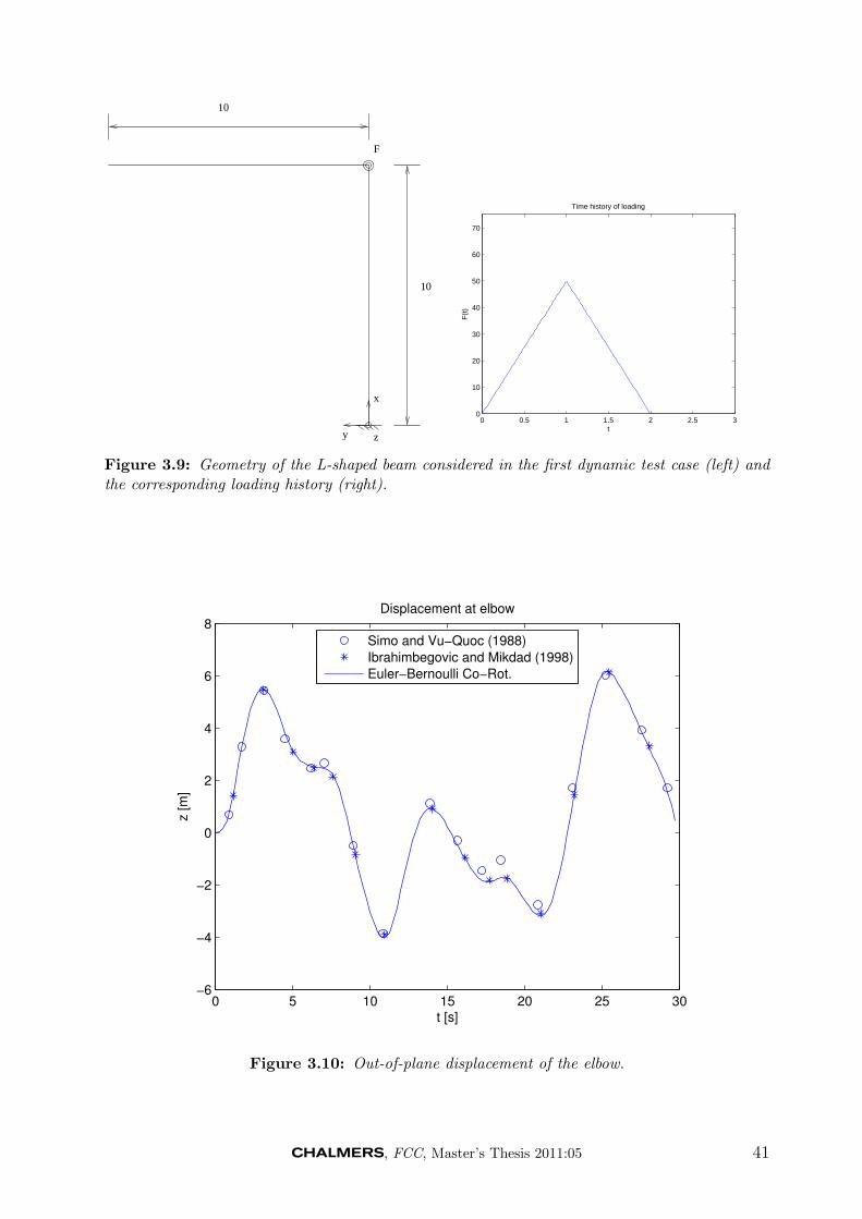
F

10

10

x

y z

0 0.5 1 1.5 2 2.5 30

10

20

30

40

50

60

70

Time history of loading

F(t

)

t

Figure 3.9: Geometry of the L-shaped beam considered in the first dynamic test case (left) andthe corresponding loading history (right).

0 5 10 15 20 25 30−6

−4

−2

0

2

4

6

8Displacement at elbow

t [s]

z [

m]

Simo and Vu−Quoc (1988)

Ibrahimbegovic and Mikdad (1998)


Figure 3.10: Out-of-plane displacement of the elbow.


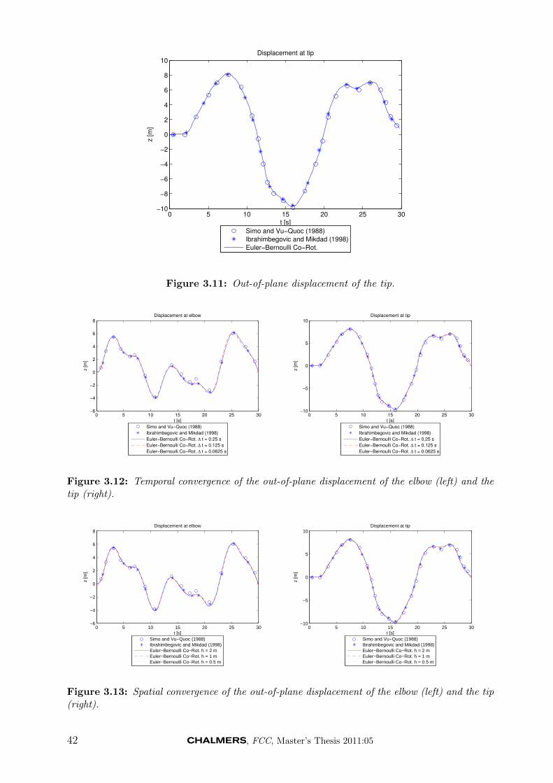
0 5 10 15 20 25 30−10

−8

−6

−4

−2

0

2

4

6

8

10Displacement at tip

t [s]

z [m

]




Figure 3.11: Out-of-plane displacement of the tip.

0 5 10 15 20 25 30−6

−4

−2

0

2

4

6


t [s]

z [

m]



Euler−Bernoulli Co−Rot. ∆ t = 0.25 s



0 5 10 15 20 25 30−10

−5

0

5


t [s]

z [

m]






Figure 3.12: Temporal convergence of the out-of-plane displacement of the elbow (left) and thetip (right).

0 5 10 15 20 25 30−6

−4

−2

0

2

4

6


t [s]

z [m

]

Simo and Vu−Quoc (1988)Ibrahimbegovic and Mikdad (1998)Euler−Bernoulli Co−Rot. h = 2 mEuler−Bernoulli Co−Rot. h = 1 mEuler−Bernoulli Co−Rot. h = 0.5 m

0 5 10 15 20 25 30−10

−5

0

5


t [s]

z [m

]

Simo and Vu−Quoc (1988)Ibrahimbegovic and Mikdad (1998)Euler−Bernoulli Co−Rot. h = 2 mEuler−Bernoulli Co−Rot. h = 1 mEuler−Bernoulli Co−Rot. h = 0.5 m

Figure 3.13: Spatial convergence of the out-of-plane displacement of the elbow (left) and the tip(right).


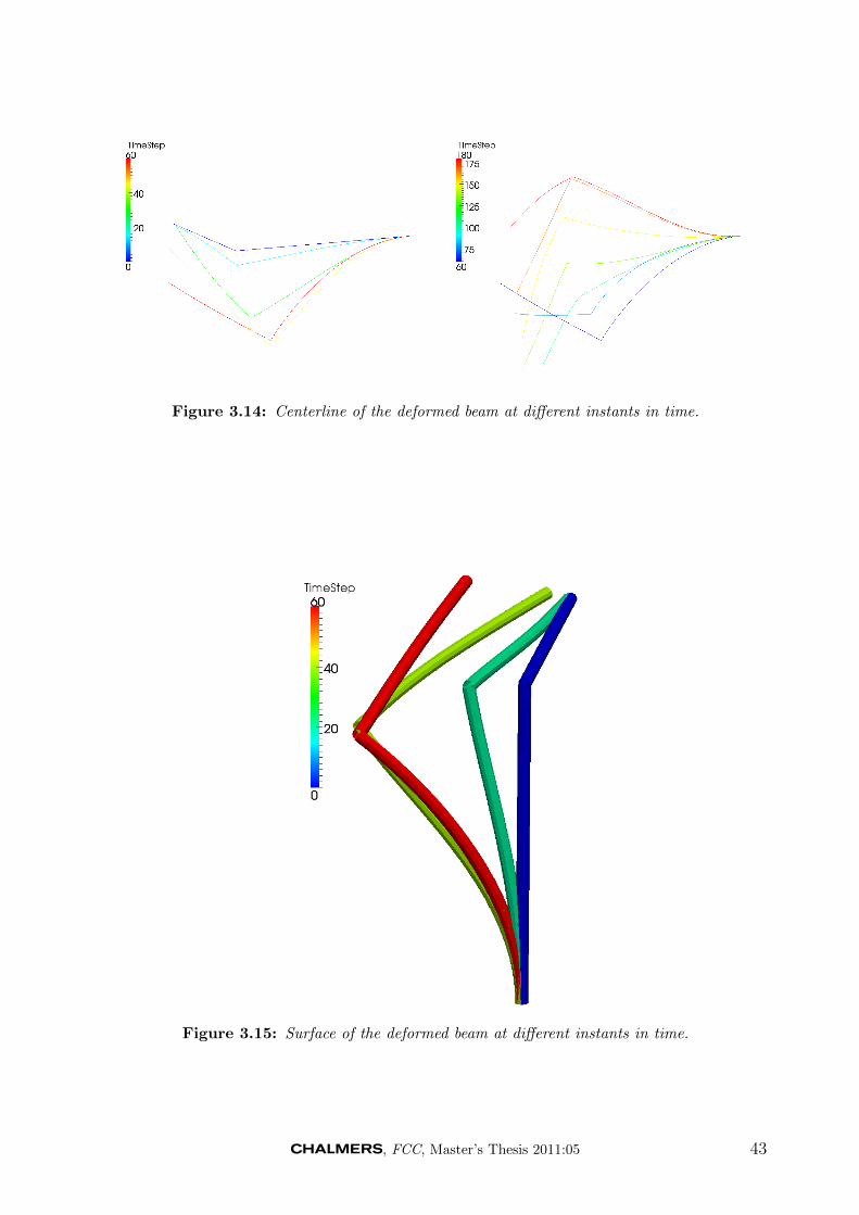
Figure 3.14: Centerline of the deformed beam at different instants in time.

Figure 3.15: Surface of the deformed beam at different instants in time.


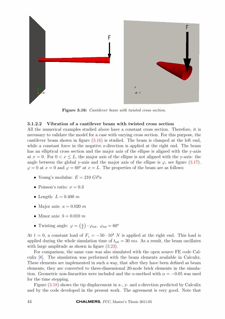
Figure 3.16: Cantilever beam with twisted cross section.

3.1.2.2 Vibration of a cantilever beam with twisted cross sectionAll the numerical examples studied above have a constant cross section. Therefore, it isnecessary to validate the model for a case with varying cross section. For this purpose, thecantilever beam shown in figure (3.16) is studied. The beam is clamped at the left end,while a constant force in the negative z-direction is applied at the right end. The beamhas an elliptical cross section and the major axis of the ellipse is aligned with the y-axisat x = 0. For 0 < x ≤ L, the major axis of the ellipse is not aligned with the y-axis: theangle between the global y-axis and the major axis of the ellipse is ϕ, see figure (3.17).ϕ = 0 at x = 0 and ϕ = 60o at x = L. The properties of the beam are as follows:

• Young’s modulus: E = 210 GPa

• Poisson’s ratio: ν = 0.3

• Length: L = 0.400 m

• Major axis: a = 0.020 m

• Minor axis: b = 0.010 m

• Twisting angle: ϕ =(xL

)· ϕtot, ϕtot = 60o

At t = 0, a constant load of Fz = −50 · 103 N is applied at the right end. This load isapplied during the whole simulation time of ttot = 30 ms. As a result, the beam oscillateswith large amplitude as shown in figure (3.23).

For comparison, the same case was also simulated with the open source FE code Cal-culix [8]. The simulation was performed with the beam elements available in Calculix.These elements are implemented in such a way, that after they have been defined as beamelements, they are converted to three-dimensional 20-node brick elements in the simula-tion. Geometric non-linearities were included and the α-method with α = −0.05 was usedfor the time stepping.

Figure (3.18) shows the tip displacement in x-, y- and z-direction predicted by Calculixand by the code developed in the present work. The agreement is very good. Note that


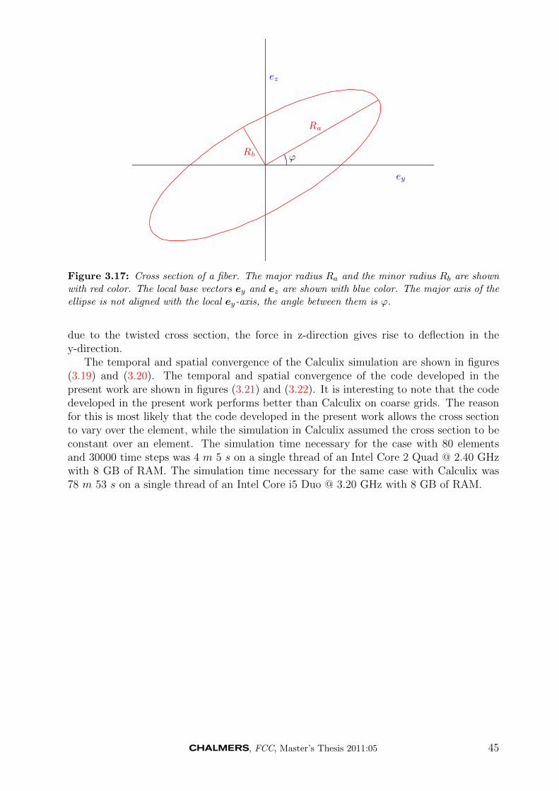
Ra

Rb

ey

ez

ϕ

Figure 3.17: Cross section of a fiber. The major radius Ra and the minor radius Rb are shownwith red color. The local base vectors ey and ez are shown with blue color. The major axis of theellipse is not aligned with the local ey-axis, the angle between them is ϕ.

due to the twisted cross section, the force in z-direction gives rise to deflection in they-direction.

The temporal and spatial convergence of the Calculix simulation are shown in figures(3.19) and (3.20). The temporal and spatial convergence of the code developed in thepresent work are shown in figures (3.21) and (3.22). It is interesting to note that the codedeveloped in the present work performs better than Calculix on coarse grids. The reasonfor this is most likely that the code developed in the present work allows the cross sectionto vary over the element, while the simulation in Calculix assumed the cross section to beconstant over an element. The simulation time necessary for the case with 80 elementsand 30000 time steps was 4 m 5 s on a single thread of an Intel Core 2 Quad @ 2.40 GHzwith 8 GB of RAM. The simulation time necessary for the same case with Calculix was78 m 53 s on a single thread of an Intel Core i5 Duo @ 3.20 GHz with 8 GB of RAM.


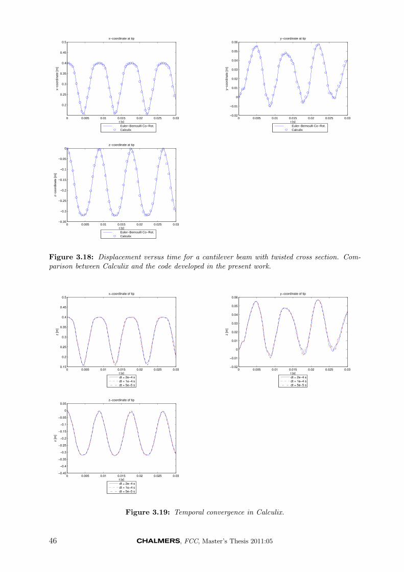
0 0.005 0.01 0.015 0.02 0.025 0.03

0.2

0.25

0.3

0.35

0.4

0.45

0.5x−coordinate at tip

t [s]

x−co

ordi

nate

[m]

Euler−Bernoulli Co−Rot.Calculix

0 0.005 0.01 0.015 0.02 0.025 0.03−0.02

−0.01

0

0.01

0.02

0.03

0.04

0.05

0.06y−coordinate at tip

t [s]

y−co

ordi

nate

[m]


0 0.005 0.01 0.015 0.02 0.025 0.03−0.35

−0.3

−0.25

−0.2

−0.15

−0.1

−0.05

0z−coordinate at tip

t [s]

z−co

ordi

nate

[m]


Figure 3.18: Displacement versus time for a cantilever beam with twisted cross section. Com-parison between Calculix and the code developed in the present work.

0 0.005 0.01 0.015 0.02 0.025 0.030.15

0.2

0.25

0.3

0.35

0.4

0.45

0.5x−coordinate of tip

t [s]

z [

m]

dt = 2e−4 s

dt = 1e−4 s

dt = 5e−5 s

0 0.005 0.01 0.015 0.02 0.025 0.03−0.02

−0.01

0

0.01

0.02

0.03

0.04

0.05

0.06y−coordinate of tip

t [s]

z [

m]

dt = 2e−4 s

dt = 1e−4 s

dt = 5e−5 s

0 0.005 0.01 0.015 0.02 0.025 0.03−0.45

−0.4

−0.35

−0.3

−0.25

−0.2

−0.15

−0.1

−0.05

0

0.05z−coordinate of tip

t [s]

z [

m]

dt = 2e−4 s

dt = 1e−4 s

dt = 5e−5 s

Figure 3.19: Temporal convergence in Calculix.


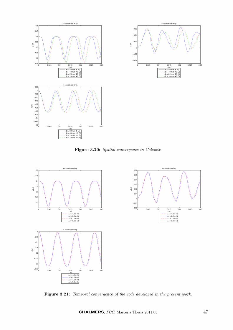
0 0.005 0.01 0.015 0.02 0.025 0.030.15

0.2

0.25

0.3

0.35

0.4

0.45


t [s]

z [

m]

dx = 80 mm (5 El)

dx = 40 mm (10 El)

dx = 20 mm (20 El)

dx = 10 mm (40 El)

0 0.005 0.01 0.015 0.02 0.025 0.03

−0.04

−0.02

0

0.02

0.04

0.06

y−coordinate of tip

t [s]

z [

m]

dx = 80 mm (5 El)

dx = 40 mm (10 El)

dx = 20 mm (20 El)

dx = 10 mm (40 El)

0 0.005 0.01 0.015 0.02 0.025 0.03−0.5

−0.45

−0.4

−0.35

−0.3

−0.25

−0.2

−0.15

−0.1

−0.05

0

0.05z−coordinate of tip

t [s]

z [

m]

dx = 80 mm (5 El)

dx = 40 mm (10 El)

dx = 20 mm (20 El)

dx = 10 mm (40 El)

Figure 3.20: Spatial convergence in Calculix.

0 0.005 0.01 0.015 0.02 0.025 0.03

0.2

0.25

0.3

0.35

0.4

0.45

0.5

t [s]

x [m

]

x−coordinate of tip

∆ t = 4.0e−4 s

∆ t = 2.0e−4 s

∆ t = 1.0e−4 s

∆ t = 5.0e−5 s

0 0.005 0.01 0.015 0.02 0.025 0.03−0.02

−0.01

0

0.01

0.02

0.03

0.04

0.05


t [s]

y [m

]

∆ t = 4.0e−4 s

∆ t = 2.0e−4 s

∆ t = 1.0e−4 s

∆ t = 5.0e−5 s

0 0.005 0.01 0.015 0.02 0.025 0.03−0.35

−0.3

−0.25

−0.2

−0.15

−0.1

−0.05

0z−coordinate of tip

t [s]

z [m

]

∆ t = 4.0e−4 s

∆ t = 2.0e−4 s

∆ t = 1.0e−4 s

∆ t = 5.0e−5 s

Figure 3.21: Temporal convergence of the code developed in the present work.


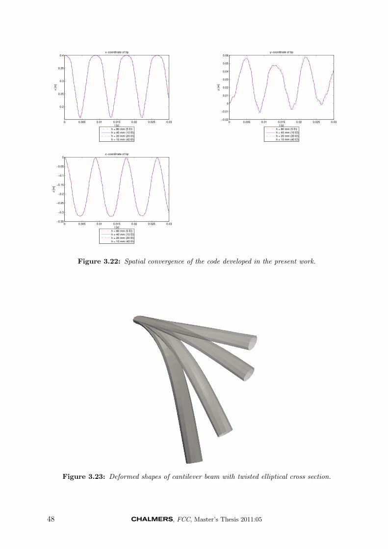
0 0.005 0.01 0.015 0.02 0.025 0.03

0.2

0.25

0.3

0.35


t [s]

x [m

]

h = 80 mm (5 El)

h = 40 mm (10 El)

h = 20 mm (20 El)

h = 10 mm (40 El)

0 0.005 0.01 0.015 0.02 0.025 0.03−0.02

−0.01

0

0.01

0.02

0.03

0.04

0.05


t [s]

y [m

]

h = 80 mm (5 El)

h = 40 mm (10 El)

h = 20 mm (20 El)

h = 10 mm (40 El)

0 0.005 0.01 0.015 0.02 0.025 0.03−0.35

−0.3

−0.25

−0.2

−0.15

−0.1

−0.05

0z−coordinate of tip

t [s]

z [m

]

h = 80 mm (5 El)

h = 40 mm (10 El)

h = 20 mm (20 El)

h = 10 mm (40 El)

Figure 3.22: Spatial convergence of the code developed in the present work.

Figure 3.23: Deformed shapes of cantilever beam with twisted elliptical cross section.


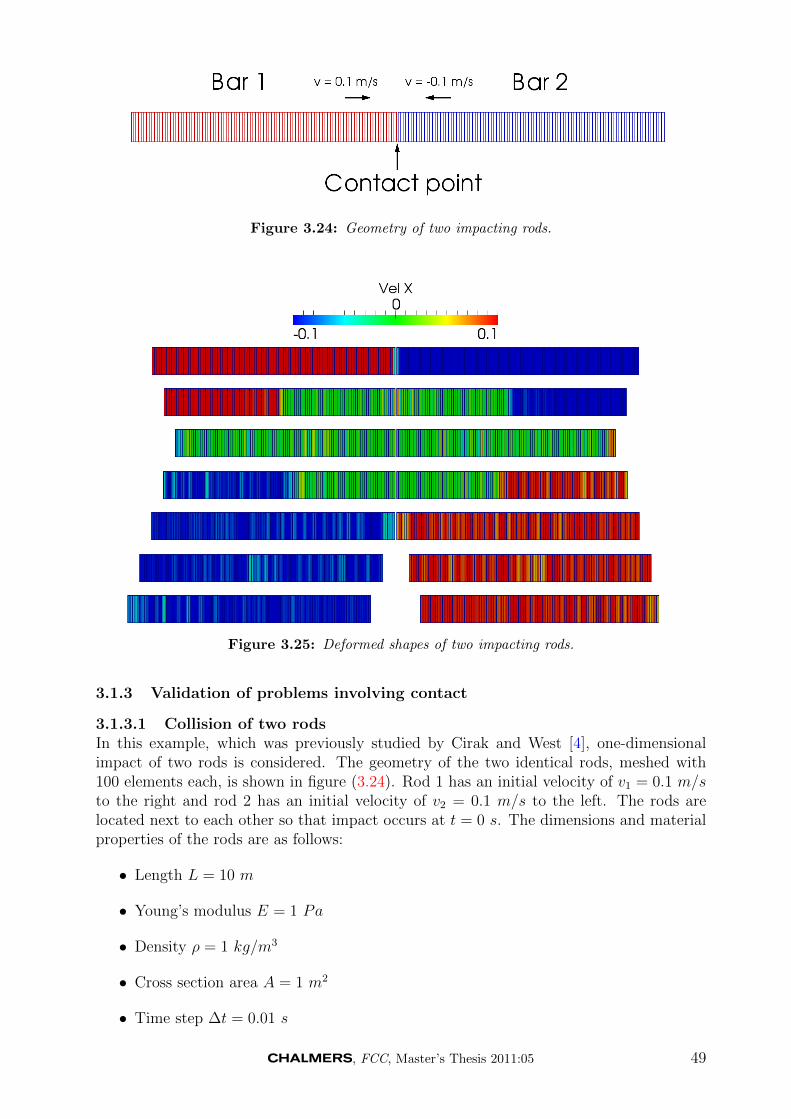
Figure 3.24: Geometry of two impacting rods.

Figure 3.25: Deformed shapes of two impacting rods.

3.1.3 Validation of problems involving contact

3.1.3.1 Collision of two rodsIn this example, which was previously studied by Cirak and West [4], one-dimensionalimpact of two rods is considered. The geometry of the two identical rods, meshed with100 elements each, is shown in figure (3.24). Rod 1 has an initial velocity of v1 = 0.1 m/sto the right and rod 2 has an initial velocity of v2 = 0.1 m/s to the left. The rods arelocated next to each other so that impact occurs at t = 0 s. The dimensions and materialproperties of the rods are as follows:

• Length L = 10 m

• Young’s modulus E = 1 Pa

• Density ρ = 1 kg/m3

• Cross section area A = 1 m2

• Time step ∆t = 0.01 s


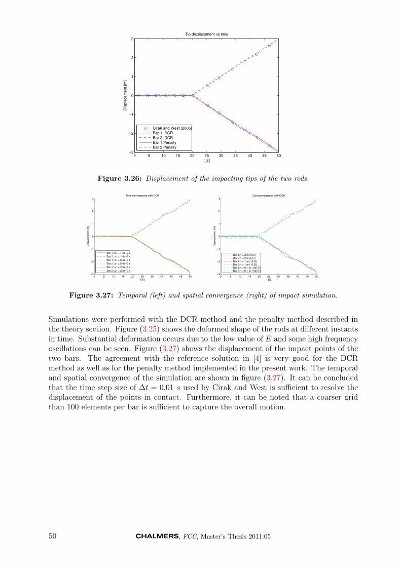
0 5 10 15 20 25 30 35 40 45 50−3

−2

−1

0

1

2

3Tip displacement vs time

t [s]

Dis

pla

cem

ent [m

]

Cirak and West (2005)

Bar 1: DCR

Bar 2: DCR

Bar 1:Penalty

Bar 2:Penalty

Figure 3.26: Displacement of the impacting tips of the two rods.

0 5 10 15 20 25 30 35 40 45 50−3

−2

−1

0

1

2

3

t [s]

Dis

pla

cem

ent [m

]

Time convergence with DCR

Bar 1: ∆ t = 1.0e−2 s

Bar 2: ∆ t = 1.0e−2 s

Bar 1: ∆ t = 5.0e−3 s

Bar 2: ∆ t = 5.0e−3 s

Bar 1: ∆ t = 2.5e−3 s

Bar 2: ∆ t = 2.5e−3 s

0 5 10 15 20 25 30 35 40 45 50−3

−2

−1

0

1

2

3Grid convergence with DCR

t [s]

Dis

pla

cem

ent [m

]

Bar 1:h = 2 m (5 El)

Bar 2:h = 2 m (5 El)

Bar 1:h = 1 m (10 El)

Bar 2:h = 1 m (10 El)

Bar 1:h = 0.1 m (100 El)

Bar 2:h = 0.1 m (100 El)

Figure 3.27: Temporal (left) and spatial convergence (right) of impact simulation.

Simulations were performed with the DCR method and the penalty method described inthe theory section. Figure (3.25) shows the deformed shape of the rods at different instantsin time. Substantial deformation occurs due to the low value of E and some high frequencyoscillations can be seen. Figure (3.27) shows the displacement of the impact points of thetwo bars. The agreement with the reference solution in [4] is very good for the DCRmethod as well as for the penalty method implemented in the present work. The temporaland spatial convergence of the simulation are shown in figure (3.27). It can be concludedthat the time step size of ∆t = 0.01 s used by Cirak and West is sufficient to resolve thedisplacement of the points in contact. Furthermore, it can be noted that a coarser gridthan 100 elements per bar is sufficient to capture the overall motion.


3.1.3.2 Impact between spinning rod and tableThe last validation case is a spinning rod falling onto a table. This problem, which involvesfricton and inelastic contact, was previously studied by Stewart and Trinkle [30]. The rodshown in figure (3.28) is released from a height of 1 m with an angle of 30o to the horizontal.Initially, the center of mass of the rod has no translational velocity, but the initial angularvelocity is 4 rad/s about the center of mass. Gravity causes the rod to fall downwardsand impact the table located at y = 0. The table is rigid and the coefficient of frictionfor the contact between the rod and the table is µfr = 0.6. The impacts are considered tobe inelastic with ecor = 0. The length of the rod excluding the rounded ends is l = 0.5 mand it has a radius of r = 0.05 m. The mass of the rod is 1 kg and its moment of inertiawith respect to the center of gravity is J = 0.002 kgm2. Stewart and Trinkle studied arigid rod. The code developed in the present work deals with elastic problems and can notsimulate perfectly rigid objects. Instead, the rod was meshed with one element and thematerial parameters of steel were used (E = 210 GPa, ν = 0.3). In this way, the rod willbehave as almost rigid in the simulations.

The initial angular velocity causes the rod to rotate as it falls towards the table. Itimpacts the table with one of its ends and continues to rotate towards the table with itsother end. Eventually the other end hits the table and the rod comes to rest. Figure (3.29)shows the centerline of the rod at different instants in time as it falls towards the table.Note that the rod has a radius of r = 0.05 m and therefore the centerline of the rod stopsat a distance of 0.05 m from the table.

The problem has been simulated with the penalty method and the DCR method imple-mented in the present work. When the penalty method was used, the penalty parameterwas set to K = 1.0 · 104 N . The reference length was set to dref = 5 · 10−2 m and theexponent was set to ζ = 1.0 resulting in a linear penalty force. Figure (3.30) shows acomparison with the results given by Stewart and Trinkle [30]. The agreement betweenthe penalty method and the reference solution is good. Note that this good agreement wasachieved even though a regularization of Coulomb’s law was used in this simulation. Theagreement between the DCR method and the reference solution is fair, but som discrep-ancy can be seen between t = 0.4 s and t = 0.6 s. Especially, note that the DCR methodpredicts a slightly too high vertical velocity after the first impact at t = 0.4 s. The reasonfor this could be the explicit character of the DCR method: the closest point projectionleads to an increase in internal energy, allowing for a light bounce-off when this internalenergy is released as kinetic energy.

The temporal convergence of the simulations performed is shown in figure (3.31) forthe penalty method and in figure (3.32) for the DCR method. A time step of ∆t = 62.5 µsgives a reasonable resolution for both methods. This can be compared to the results givenin [30], where a time step of 5 ms gave a solution independent of the time step length. Thereason for the difference in necessary time step length is most likely that [30] used a rigidbody code to study a rigid body problem, while the present work used an elasticity codeto study the same rigid body problem.

The simulation time for this problem with a time step of ∆t = 31.25 µs was 13.7 swith the penalty method. A time step of ∆t = 31.25 µs corresponds to 32000 time stepsand the simulation was performed on a single thread of an Intel Core 2 Quad @ 2.40 GHzwith 8 GB of RAM. The simulation time needed by the impulse based method was 16.5 swith the same settings and the same computer.


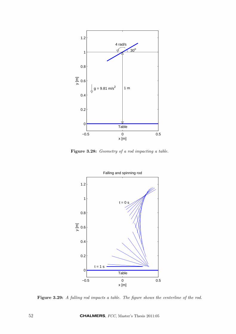
−0.5 0 0.5

0

0.2

0.4

0.6

0.8

1

1.2

x [m]

y [m

]

1 m

Table

30o

4 rad/s

g = 9.81 m/s2

Figure 3.28: Geometry of a rod impacting a table.

−0.5 0 0.5

0

0.2

0.4

0.6

0.8

1

1.2

x [m]

y [m

]

t = 0 s

t = 1 s

Falling and spinning rod

Table

Figure 3.29: A falling rod impacts a table. The figure shows the centerline of the rod.


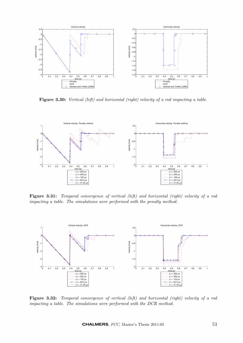
0 0.1 0.2 0.3 0.4 0.5 0.6 0.7 0.8 0.9 1−4

−3.5

−3

−2.5

−2

−1.5

−1

−0.5

0

0.5Vertical velocity

time [s]

velo

city

[m/s

]

PenaltyDCRStewart and Trinkle (1996)

0 0.1 0.2 0.3 0.4 0.5 0.6 0.7 0.8 0.9 1−1.8

−1.6

−1.4

−1.2

−1

−0.8

−0.6

−0.4

−0.2

0

0.2Horizontal velocity

time [s]

velo

city

[m/s

]

PenaltyDCRStewart and Trinkle (1996)

Figure 3.30: Vertical (left) and horizontal (right) velocity of a rod impacting a table.

0 0.1 0.2 0.3 0.4 0.5 0.6 0.7 0.8 0.9 1−4

−3

−2

−1

0

1Vertical velocity: Penalty method

time [s]

ve

locity [

m/s

]

∆ t = 500 µs

∆ t = 250 µs

∆ t = 125 µs

∆ t = 62.5 µs

∆ t = 31.25 µs

0 0.1 0.2 0.3 0.4 0.5 0.6 0.7 0.8 0.9 1−2

−1.5

−1

−0.5

0

0.5Horizontal velocity: Penalty method

time [s]

ve

locity [

m/s

]

∆ t = 500 µs

∆ t = 250 µs

∆ t = 125 µs

∆ t = 62.5 µs

∆ t = 31.25 µs

Figure 3.31: Temporal convergence of vertical (left) and horizontal (right) velocity of a rodimpacting a table. The simulations were performed with the penalty method.

0 0.1 0.2 0.3 0.4 0.5 0.6 0.7 0.8 0.9 1−4

−3

−2

−1

0

1Vertical velocity: DCR

time [s]

ve

locity [

m/s

]

∆ t = 500 µs

∆ t = 250 µs

∆ t = 125 µs

∆ t = 62.5 µs

∆ t = 31.25 µs

0 0.1 0.2 0.3 0.4 0.5 0.6 0.7 0.8 0.9 1−2

−1.5

−1

−0.5

0

0.5Horizontal velocity: DCR

time [s]

ve

locity [

m/s

]

∆ t = 500 µs

∆ t = 250 µs

∆ t = 125 µs

∆ t = 62.5 µs

∆ t = 31.25 µs

Figure 3.32: Temporal convergence of vertical (left) and horizontal (right) velocity of a rodimpacting a table. The simulations were performed with the DCR method.


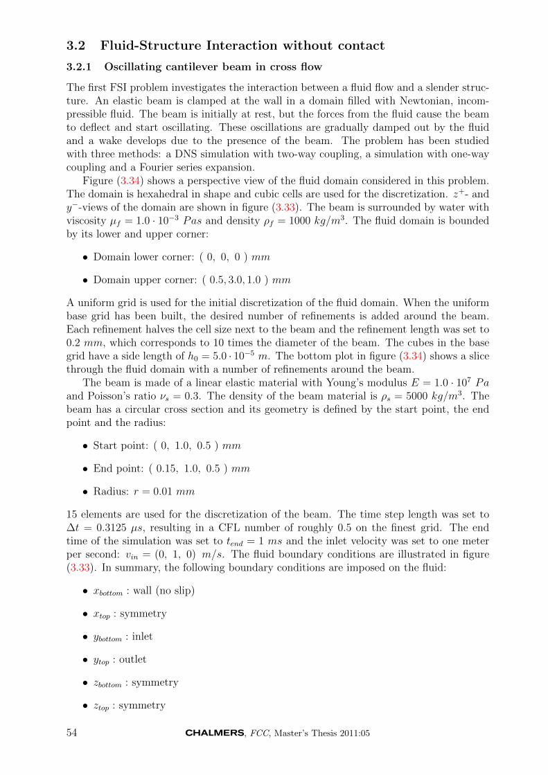
3.2 Fluid-Structure Interaction without contact

3.2.1 Oscillating cantilever beam in cross flow

The first FSI problem investigates the interaction between a fluid flow and a slender struc-ture. An elastic beam is clamped at the wall in a domain filled with Newtonian, incom-pressible fluid. The beam is initially at rest, but the forces from the fluid cause the beamto deflect and start oscillating. These oscillations are gradually damped out by the fluidand a wake develops due to the presence of the beam. The problem has been studiedwith three methods: a DNS simulation with two-way coupling, a simulation with one-waycoupling and a Fourier series expansion.

Figure (3.34) shows a perspective view of the fluid domain considered in this problem.The domain is hexahedral in shape and cubic cells are used for the discretization. z+- andy−-views of the domain are shown in figure (3.33). The beam is surrounded by water withviscosity µf = 1.0 · 10−3 Pas and density ρf = 1000 kg/m3. The fluid domain is boundedby its lower and upper corner:

• Domain lower corner: ( 0, 0, 0 ) mm

• Domain upper corner: ( 0.5, 3.0, 1.0 ) mm

A uniform grid is used for the initial discretization of the fluid domain. When the uniformbase grid has been built, the desired number of refinements is added around the beam.Each refinement halves the cell size next to the beam and the refinement length was set to0.2 mm, which corresponds to 10 times the diameter of the beam. The cubes in the basegrid have a side length of h0 = 5.0 · 10−5 m. The bottom plot in figure (3.34) shows a slicethrough the fluid domain with a number of refinements around the beam.

The beam is made of a linear elastic material with Young’s modulus E = 1.0 · 107 Paand Poisson’s ratio νs = 0.3. The density of the beam material is ρs = 5000 kg/m3. Thebeam has a circular cross section and its geometry is defined by the start point, the endpoint and the radius:

• Start point: ( 0, 1.0, 0.5 ) mm

• End point: ( 0.15, 1.0, 0.5 ) mm

• Radius: r = 0.01 mm

15 elements are used for the discretization of the beam. The time step length was set to∆t = 0.3125 µs, resulting in a CFL number of roughly 0.5 on the finest grid. The endtime of the simulation was set to tend = 1 ms and the inlet velocity was set to one meterper second: vin = (0, 1, 0) m/s. The fluid boundary conditions are illustrated in figure(3.33). In summary, the following boundary conditions are imposed on the fluid:

• xbottom : wall (no slip)

• xtop : symmetry

• ybottom : inlet

• ytop : outlet

• zbottom : symmetry

• ztop : symmetry


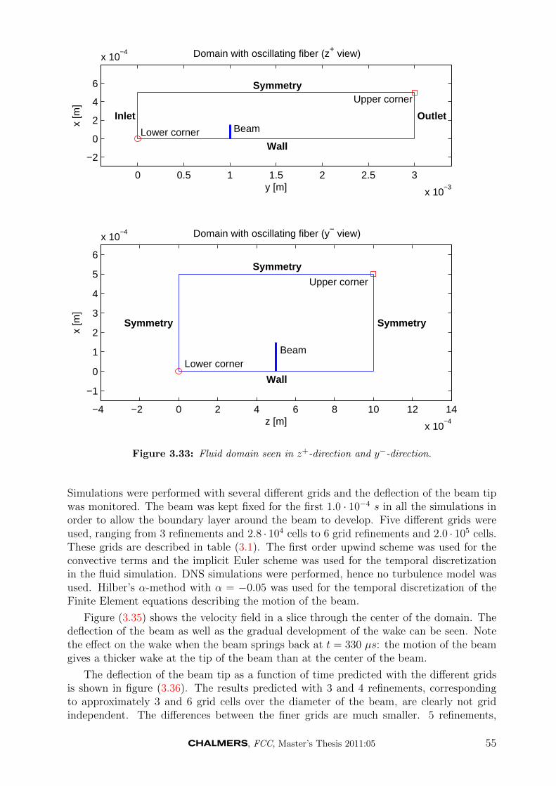
0 0.5 1 1.5 2 2.5 3

x 10−3

−2

0

2

4

6

x 10−4

Lower corner

Upper corner

BeamInlet Outlet

Wall

Symmetry

y [m]

x [m

]

Domain with oscillating fiber (z+ view)

−4 −2 0 2 4 6 8 10 12 14

x 10−4

−1

0

1

2

3

4

5

6

x 10−4

Lower corner

Upper corner

Beam

Wall

Symmetry

Symmetry Symmetry

z [m]

x [m

]

Domain with oscillating fiber (y− view)

Figure 3.33: Fluid domain seen in z+-direction and y−-direction.

Simulations were performed with several different grids and the deflection of the beam tipwas monitored. The beam was kept fixed for the first 1.0 · 10−4 s in all the simulations inorder to allow the boundary layer around the beam to develop. Five different grids wereused, ranging from 3 refinements and 2.8 · 104 cells to 6 grid refinements and 2.0 · 105 cells.These grids are described in table (3.1). The first order upwind scheme was used for theconvective terms and the implicit Euler scheme was used for the temporal discretizationin the fluid simulation. DNS simulations were performed, hence no turbulence model wasused. Hilber’s α-method with α = −0.05 was used for the temporal discretization of theFinite Element equations describing the motion of the beam.

Figure (3.35) shows the velocity field in a slice through the center of the domain. Thedeflection of the beam as well as the gradual development of the wake can be seen. Notethe effect on the wake when the beam springs back at t = 330 µs: the motion of the beamgives a thicker wake at the tip of the beam than at the center of the beam.

The deflection of the beam tip as a function of time predicted with the different gridsis shown in figure (3.36). The results predicted with 3 and 4 refinements, correspondingto approximately 3 and 6 grid cells over the diameter of the beam, are clearly not gridindependent. The differences between the finer grids are much smaller. 5 refinements,


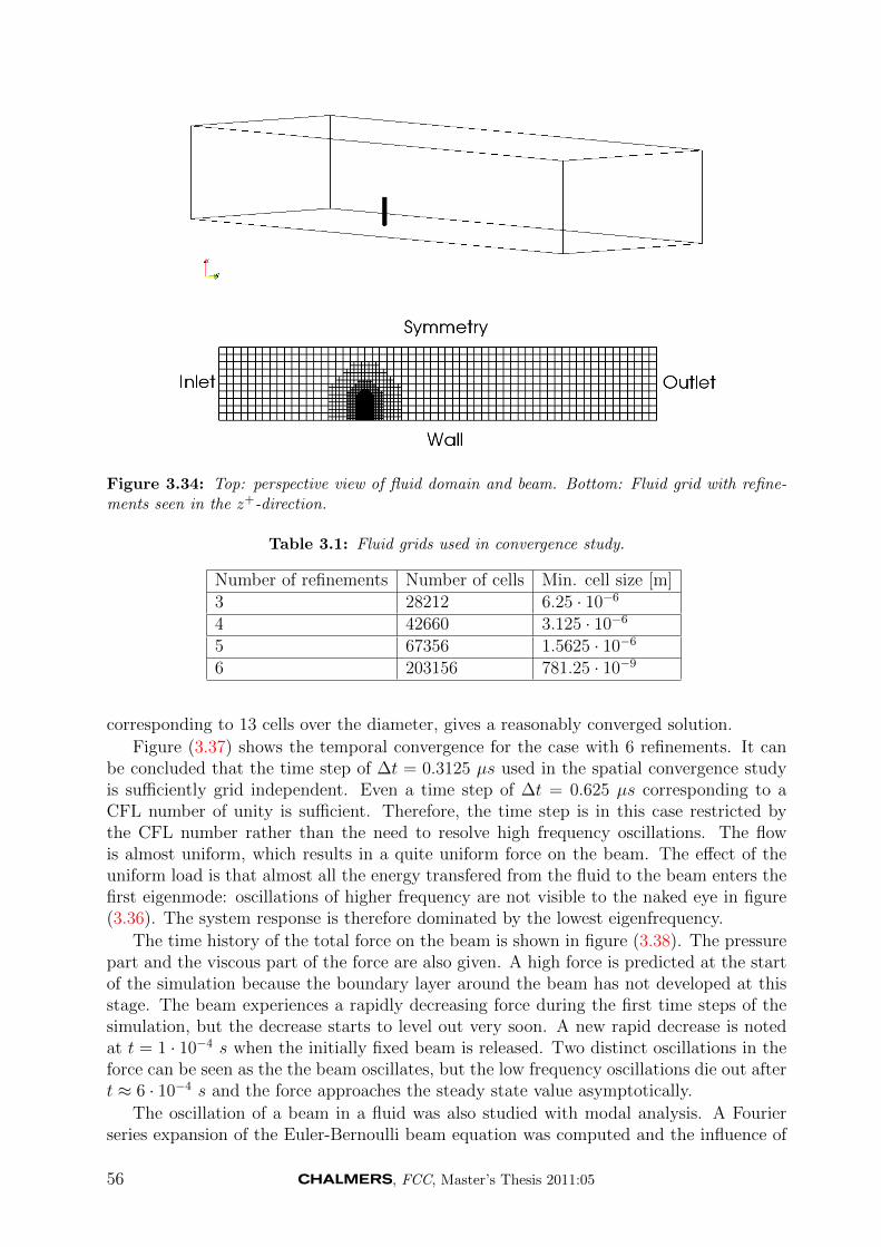
Figure 3.34: Top: perspective view of fluid domain and beam. Bottom: Fluid grid with refine-ments seen in the z+-direction.

Table 3.1: Fluid grids used in convergence study.

Number of refinements Number of cells Min. cell size [m]3 28212 6.25 · 10−6

4 42660 3.125 · 10−6

5 67356 1.5625 · 10−6

6 203156 781.25 · 10−9

corresponding to 13 cells over the diameter, gives a reasonably converged solution.

Figure (3.37) shows the temporal convergence for the case with 6 refinements. It canbe concluded that the time step of ∆t = 0.3125 µs used in the spatial convergence studyis sufficiently grid independent. Even a time step of ∆t = 0.625 µs corresponding to aCFL number of unity is sufficient. Therefore, the time step is in this case restricted bythe CFL number rather than the need to resolve high frequency oscillations. The flowis almost uniform, which results in a quite uniform force on the beam. The effect of theuniform load is that almost all the energy transfered from the fluid to the beam enters thefirst eigenmode: oscillations of higher frequency are not visible to the naked eye in figure(3.36). The system response is therefore dominated by the lowest eigenfrequency.

The time history of the total force on the beam is shown in figure (3.38). The pressurepart and the viscous part of the force are also given. A high force is predicted at the startof the simulation because the boundary layer around the beam has not developed at thisstage. The beam experiences a rapidly decreasing force during the first time steps of thesimulation, but the decrease starts to level out very soon. A new rapid decrease is notedat t = 1 · 10−4 s when the initially fixed beam is released. Two distinct oscillations in theforce can be seen as the the beam oscillates, but the low frequency oscillations die out aftert ≈ 6 · 10−4 s and the force approaches the steady state value asymptotically.

The oscillation of a beam in a fluid was also studied with modal analysis. A Fourierseries expansion of the Euler-Bernoulli beam equation was computed and the influence of


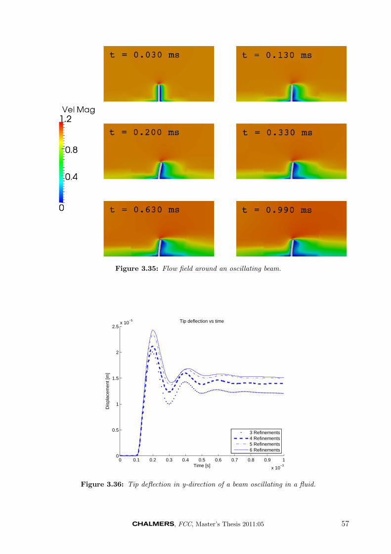
Figure 3.35: Flow field around an oscillating beam.

0 0.1 0.2 0.3 0.4 0.5 0.6 0.7 0.8 0.9 1

x 10−3

0

0.5

1

1.5

2

2.5x 10

−5 Tip deflection vs time

Time [s]

Dis

plac

emen

t [m

]

3 Refinements4 Refinements5 Refinements6 Refinements

Figure 3.36: Tip deflection in y-direction of a beam oscillating in a fluid.


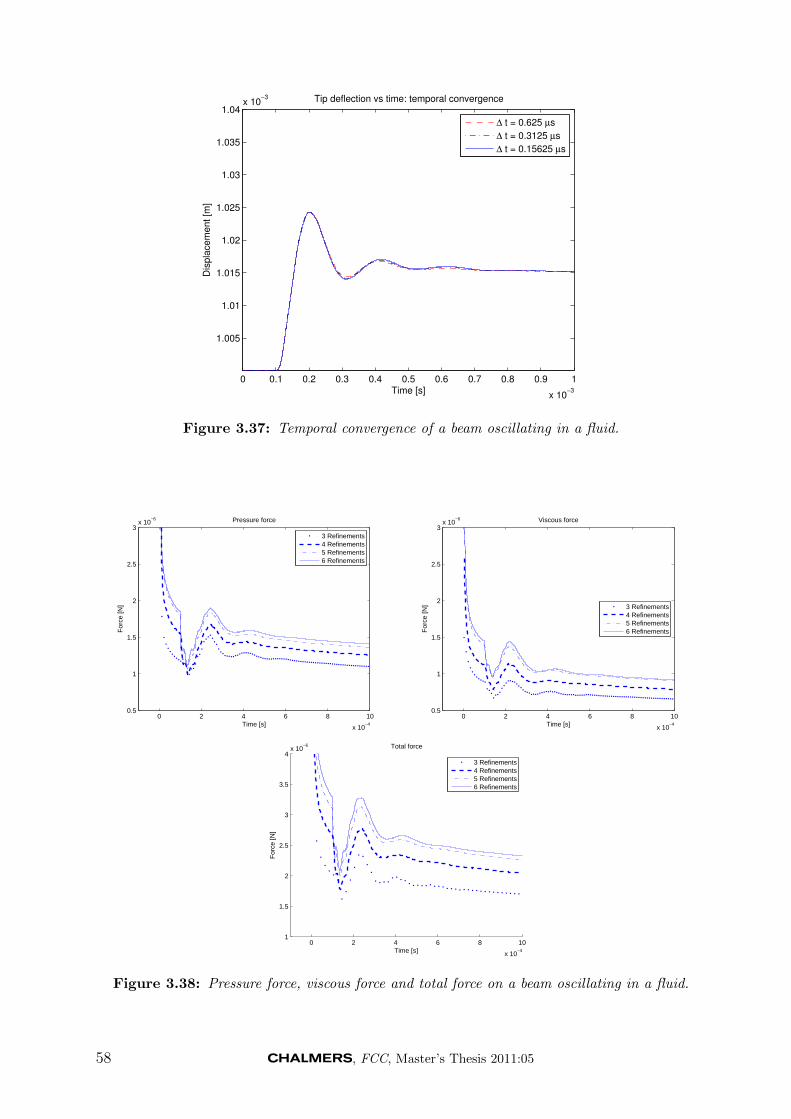
0 0.1 0.2 0.3 0.4 0.5 0.6 0.7 0.8 0.9 1

x 10−3

1.005

1.01

1.015

1.02

1.025

1.03

1.035

1.04x 10

−3 Tip deflection vs time: temporal convergence

Time [s]

Dis

pla

cem

ent [m

]

∆ t = 0.625 µs

∆ t = 0.3125 µs

∆ t = 0.15625 µs

Figure 3.37: Temporal convergence of a beam oscillating in a fluid.

0 2 4 6 8 10

x 10−4

0.5

1

1.5

2

2.5

3x 10

−6 Pressure force

Time [s]

For

ce [N

]


0 2 4 6 8 10

x 10−4

0.5

1

1.5

2

2.5

3x 10

−6 Viscous force

Time [s]

For

ce [N

]


0 2 4 6 8 10

x 10−4

1

1.5

2

2.5

3

3.5

4x 10

−6 Total force

Time [s]

For

ce [N

]


Figure 3.38: Pressure force, viscous force and total force on a beam oscillating in a fluid.


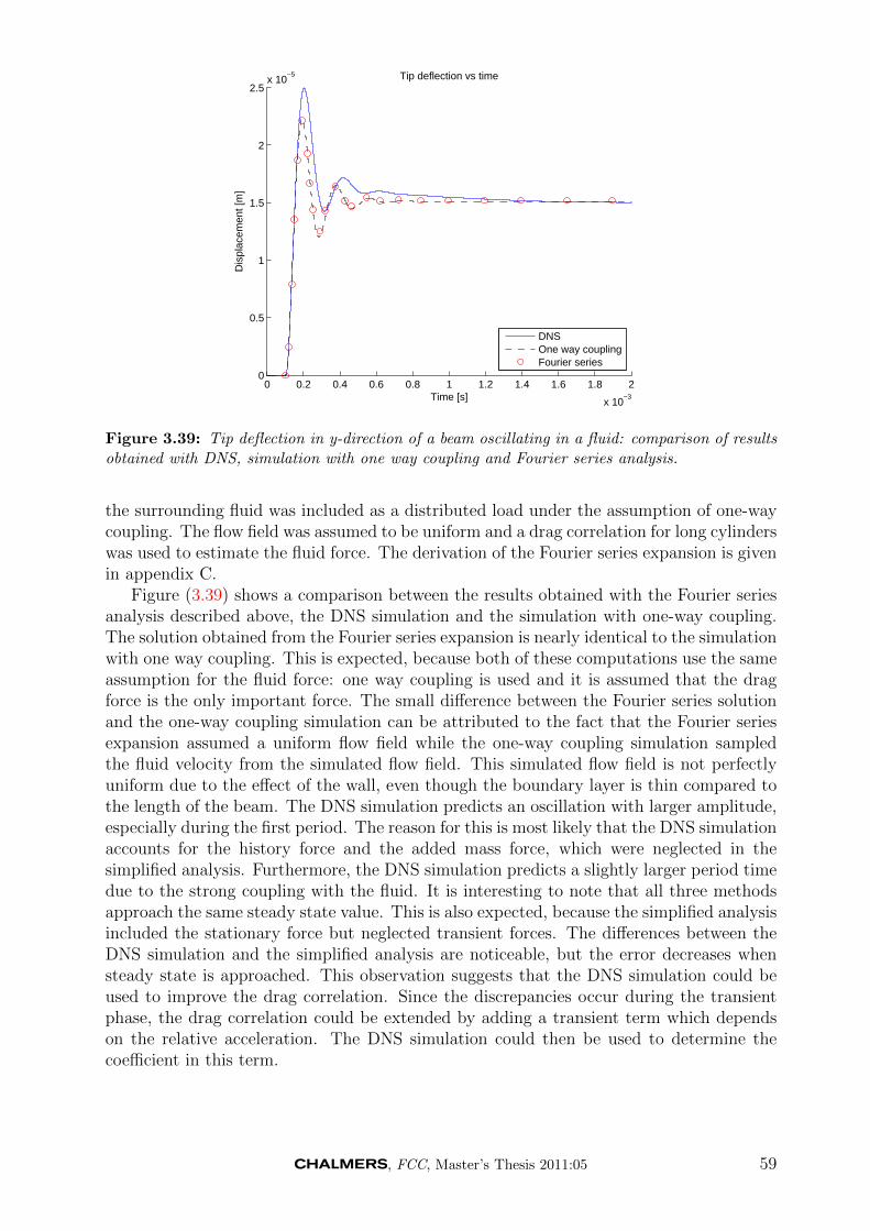
0 0.2 0.4 0.6 0.8 1 1.2 1.4 1.6 1.8 2

x 10−3

0

0.5

1

1.5

2

2.5x 10

−5 Tip deflection vs time

Time [s]

Dis

plac

emen

t [m

]

DNSOne way couplingFourier series

Figure 3.39: Tip deflection in y-direction of a beam oscillating in a fluid: comparison of resultsobtained with DNS, simulation with one way coupling and Fourier series analysis.

the surrounding fluid was included as a distributed load under the assumption of one-waycoupling. The flow field was assumed to be uniform and a drag correlation for long cylinderswas used to estimate the fluid force. The derivation of the Fourier series expansion is givenin appendix C.

Figure (3.39) shows a comparison between the results obtained with the Fourier seriesanalysis described above, the DNS simulation and the simulation with one-way coupling.The solution obtained from the Fourier series expansion is nearly identical to the simulationwith one way coupling. This is expected, because both of these computations use the sameassumption for the fluid force: one way coupling is used and it is assumed that the dragforce is the only important force. The small difference between the Fourier series solutionand the one-way coupling simulation can be attributed to the fact that the Fourier seriesexpansion assumed a uniform flow field while the one-way coupling simulation sampledthe fluid velocity from the simulated flow field. This simulated flow field is not perfectlyuniform due to the effect of the wall, even though the boundary layer is thin compared tothe length of the beam. The DNS simulation predicts an oscillation with larger amplitude,especially during the first period. The reason for this is most likely that the DNS simulationaccounts for the history force and the added mass force, which were neglected in thesimplified analysis. Furthermore, the DNS simulation predicts a slightly larger period timedue to the strong coupling with the fluid. It is interesting to note that all three methodsapproach the same steady state value. This is also expected, because the simplified analysisincluded the stationary force but neglected transient forces. The differences between theDNS simulation and the simplified analysis are noticeable, but the error decreases whensteady state is approached. This observation suggests that the DNS simulation could beused to improve the drag correlation. Since the discrepancies occur during the transientphase, the drag correlation could be extended by adding a transient term which dependson the relative acceleration. The DNS simulation could then be used to determine thecoefficient in this term.


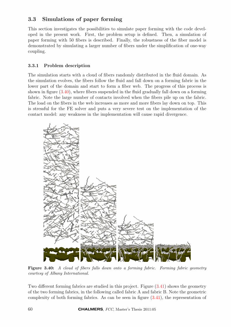
3.3 Simulations of paper forming

This section investigates the possibilities to simulate paper forming with the code devel-oped in the present work. First, the problem setup is defined. Then, a simulation ofpaper forming with 50 fibers is described. Finally, the robustness of the fiber model isdemonstrated by simulating a larger number of fibers under the simplification of one-waycoupling.

3.3.1 Problem description

The simulation starts with a cloud of fibers randomly distributed in the fluid domain. Asthe simulation evolves, the fibers follow the fluid and fall down on a forming fabric in thelower part of the domain and start to form a fiber web. The progress of this process isshown in figure (3.40), where fibers suspended in the fluid gradually fall down on a formingfabric. Note the large number of contacts involved when the fibers pile up on the fabric.The load on the fibers in the web increases as more and more fibers lay down on top. Thisis stressful for the FE solver and puts a very severe test on the implementation of thecontact model: any weakness in the implementation will cause rapid divergence.

Figure 3.40: A cloud of fibers falls down onto a forming fabric. Forming fabric geometrycourtesy of Albany International.

Two different forming fabrics are studied in this project. Figure (3.41) shows the geometryof the two forming fabrics, in the following called fabric A and fabric B. Note the geometriccomplexity of both forming fabrics. As can be seen in figure (3.41), the representation of


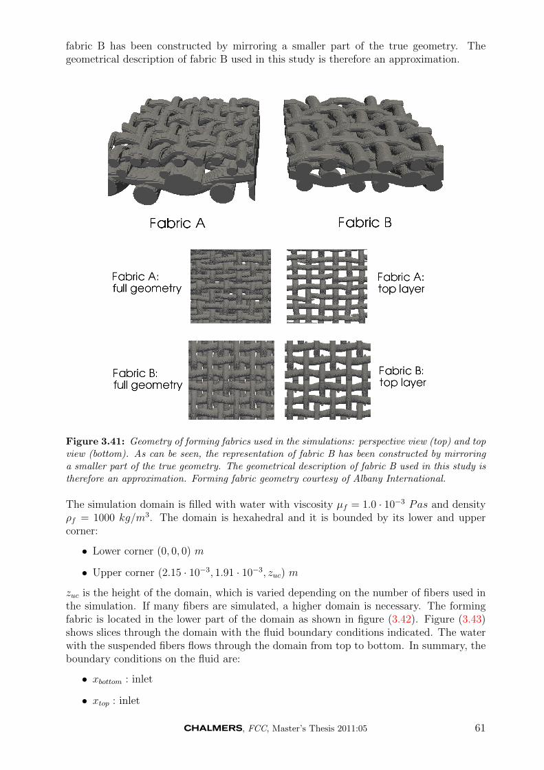
fabric B has been constructed by mirroring a smaller part of the true geometry. Thegeometrical description of fabric B used in this study is therefore an approximation.

Figure 3.41: Geometry of forming fabrics used in the simulations: perspective view (top) and topview (bottom). As can be seen, the representation of fabric B has been constructed by mirroringa smaller part of the true geometry. The geometrical description of fabric B used in this study istherefore an approximation. Forming fabric geometry courtesy of Albany International.

The simulation domain is filled with water with viscosity µf = 1.0 · 10−3 Pas and densityρf = 1000 kg/m3. The domain is hexahedral and it is bounded by its lower and uppercorner:

• Lower corner (0, 0, 0) m

• Upper corner (2.15 · 10−3, 1.91 · 10−3, zuc) m

zuc is the height of the domain, which is varied depending on the number of fibers used inthe simulation. If many fibers are simulated, a higher domain is necessary. The formingfabric is located in the lower part of the domain as shown in figure (3.42). Figure (3.43)shows slices through the domain with the fluid boundary conditions indicated. The waterwith the suspended fibers flows through the domain from top to bottom. In summary, theboundary conditions on the fluid are:

• xbottom : inlet

• xtop : inlet


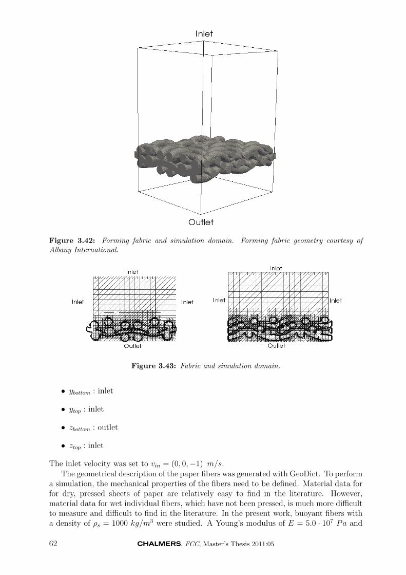
Figure 3.42: Forming fabric and simulation domain. Forming fabric geometry courtesy ofAlbany International.

Figure 3.43: Fabric and simulation domain.

• ybottom : inlet

• ytop : inlet

• zbottom : outlet

• ztop : inlet

The inlet velocity was set to vin = (0, 0,−1) m/s.The geometrical description of the paper fibers was generated with GeoDict. To perform

a simulation, the mechanical properties of the fibers need to be defined. Material data forfor dry, pressed sheets of paper are relatively easy to find in the literature. However,material data for wet individual fibers, which have not been pressed, is much more difficultto measure and difficult to find in the literature. In the present work, buoyant fibers witha density of ρs = 1000 kg/m3 were studied. A Young’s modulus of E = 5.0 · 107 Pa and


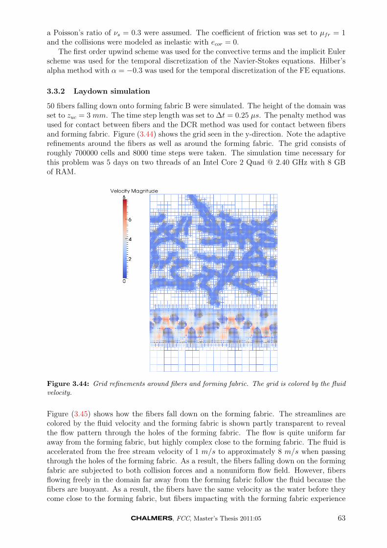
a Poisson’s ratio of νs = 0.3 were assumed. The coefficient of friction was set to µfr = 1and the collisions were modeled as inelastic with ecor = 0.

The first order upwind scheme was used for the convective terms and the implicit Eulerscheme was used for the temporal discretization of the Navier-Stokes equations. Hilber’salpha method with α = −0.3 was used for the temporal discretization of the FE equations.

3.3.2 Laydown simulation

50 fibers falling down onto forming fabric B were simulated. The height of the domain wasset to zuc = 3 mm. The time step length was set to ∆t = 0.25 µs. The penalty method wasused for contact between fibers and the DCR method was used for contact between fibersand forming fabric. Figure (3.44) shows the grid seen in the y-direction. Note the adaptiverefinements around the fibers as well as around the forming fabric. The grid consists ofroughly 700000 cells and 8000 time steps were taken. The simulation time necessary forthis problem was 5 days on two threads of an Intel Core 2 Quad @ 2.40 GHz with 8 GBof RAM.

Figure 3.44: Grid refinements around fibers and forming fabric. The grid is colored by the fluidvelocity.

Figure (3.45) shows how the fibers fall down on the forming fabric. The streamlines arecolored by the fluid velocity and the forming fabric is shown partly transparent to revealthe flow pattern through the holes of the forming fabric. The flow is quite uniform faraway from the forming fabric, but highly complex close to the forming fabric. The fluid isaccelerated from the free stream velocity of 1 m/s to approximately 8 m/s when passingthrough the holes of the forming fabric. As a result, the fibers falling down on the formingfabric are subjected to both collision forces and a nonuniform flow field. However, fibersflowing freely in the domain far away from the forming fabric follow the fluid because thefibers are buoyant. As a result, the fibers have the same velocity as the water before theycome close to the forming fabric, but fibers impacting with the forming fabric experience


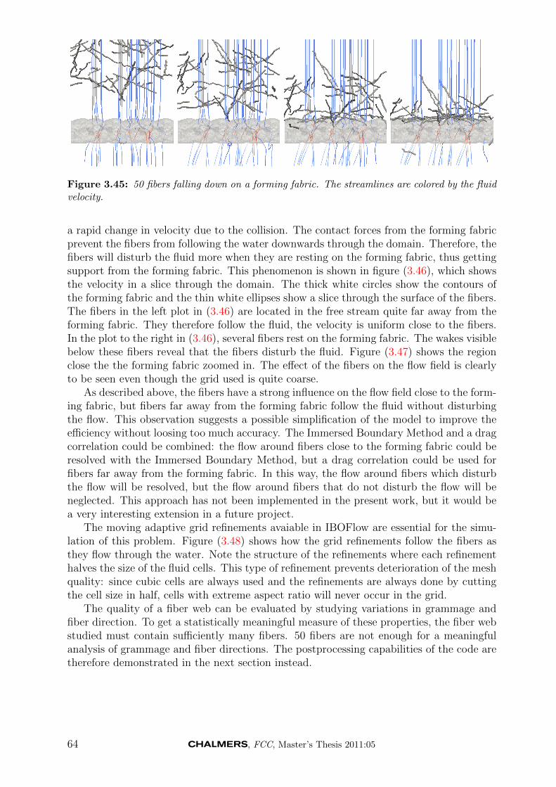
Figure 3.45: 50 fibers falling down on a forming fabric. The streamlines are colored by the fluidvelocity.

a rapid change in velocity due to the collision. The contact forces from the forming fabricprevent the fibers from following the water downwards through the domain. Therefore, thefibers will disturb the fluid more when they are resting on the forming fabric, thus gettingsupport from the forming fabric. This phenomenon is shown in figure (3.46), which showsthe velocity in a slice through the domain. The thick white circles show the contours ofthe forming fabric and the thin white ellipses show a slice through the surface of the fibers.The fibers in the left plot in (3.46) are located in the free stream quite far away from theforming fabric. They therefore follow the fluid, the velocity is uniform close to the fibers.In the plot to the right in (3.46), several fibers rest on the forming fabric. The wakes visiblebelow these fibers reveal that the fibers disturb the fluid. Figure (3.47) shows the regionclose the the forming fabric zoomed in. The effect of the fibers on the flow field is clearlyto be seen even though the grid used is quite coarse.

As described above, the fibers have a strong influence on the flow field close to the form-ing fabric, but fibers far away from the forming fabric follow the fluid without disturbingthe flow. This observation suggests a possible simplification of the model to improve theefficiency without loosing too much accuracy. The Immersed Boundary Method and a dragcorrelation could be combined: the flow around fibers close to the forming fabric could beresolved with the Immersed Boundary Method, but a drag correlation could be used forfibers far away from the forming fabric. In this way, the flow around fibers which disturbthe flow will be resolved, but the flow around fibers that do not disturb the flow will beneglected. This approach has not been implemented in the present work, but it would bea very interesting extension in a future project.

The moving adaptive grid refinements avaiable in IBOFlow are essential for the simu-lation of this problem. Figure (3.48) shows how the grid refinements follow the fibers asthey flow through the water. Note the structure of the refinements where each refinementhalves the size of the fluid cells. This type of refinement prevents deterioration of the meshquality: since cubic cells are always used and the refinements are always done by cuttingthe cell size in half, cells with extreme aspect ratio will never occur in the grid.

The quality of a fiber web can be evaluated by studying variations in grammage andfiber direction. To get a statistically meaningful measure of these properties, the fiber webstudied must contain sufficiently many fibers. 50 fibers are not enough for a meaningfulanalysis of grammage and fiber directions. The postprocessing capabilities of the code aretherefore demonstrated in the next section instead.


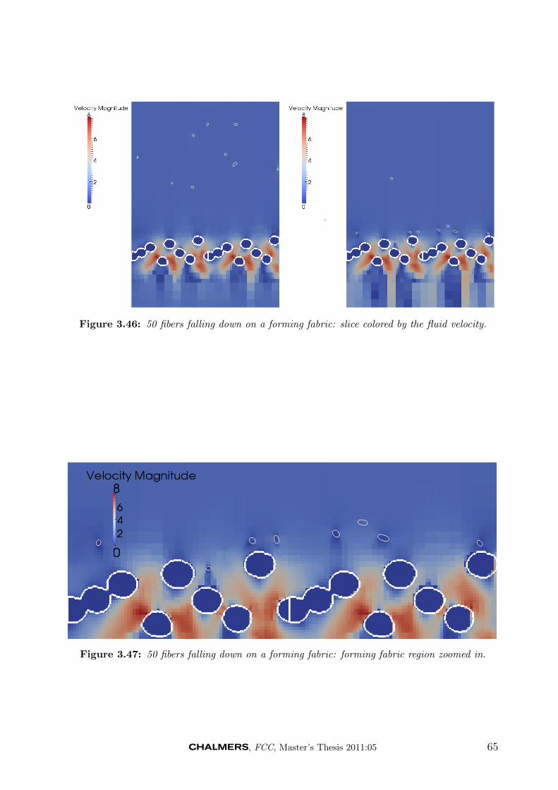
Figure 3.46: 50 fibers falling down on a forming fabric: slice colored by the fluid velocity.

Figure 3.47: 50 fibers falling down on a forming fabric: forming fabric region zoomed in.


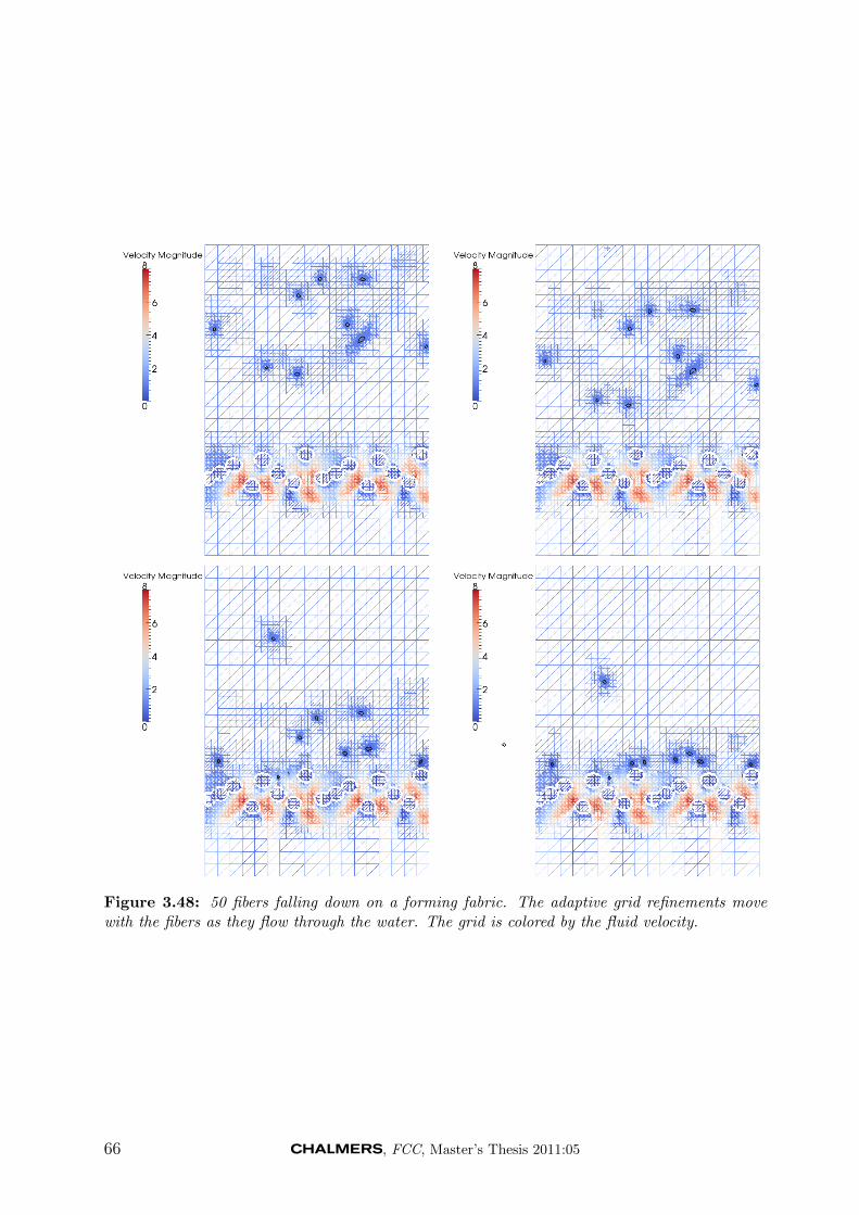
Figure 3.48: 50 fibers falling down on a forming fabric. The adaptive grid refinements movewith the fibers as they flow through the water. The grid is colored by the fluid velocity.


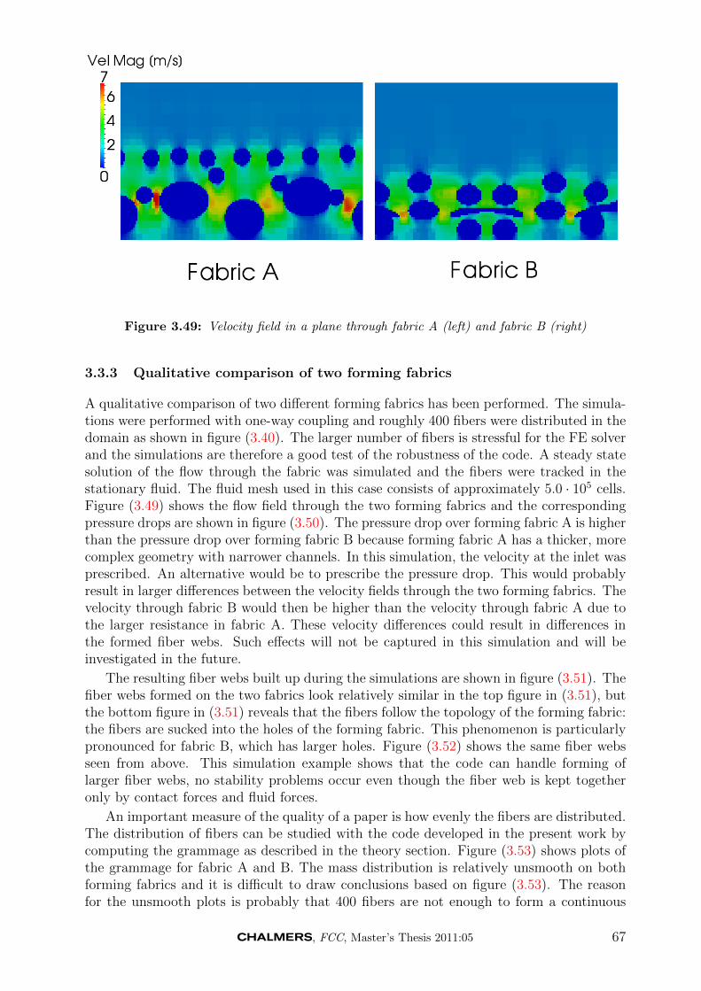
Figure 3.49: Velocity field in a plane through fabric A (left) and fabric B (right)

3.3.3 Qualitative comparison of two forming fabrics

A qualitative comparison of two different forming fabrics has been performed. The simula-tions were performed with one-way coupling and roughly 400 fibers were distributed in thedomain as shown in figure (3.40). The larger number of fibers is stressful for the FE solverand the simulations are therefore a good test of the robustness of the code. A steady statesolution of the flow through the fabric was simulated and the fibers were tracked in thestationary fluid. The fluid mesh used in this case consists of approximately 5.0 · 105 cells.Figure (3.49) shows the flow field through the two forming fabrics and the correspondingpressure drops are shown in figure (3.50). The pressure drop over forming fabric A is higherthan the pressure drop over forming fabric B because forming fabric A has a thicker, morecomplex geometry with narrower channels. In this simulation, the velocity at the inlet wasprescribed. An alternative would be to prescribe the pressure drop. This would probablyresult in larger differences between the velocity fields through the two forming fabrics. Thevelocity through fabric B would then be higher than the velocity through fabric A due tothe larger resistance in fabric A. These velocity differences could result in differences inthe formed fiber webs. Such effects will not be captured in this simulation and will beinvestigated in the future.

The resulting fiber webs built up during the simulations are shown in figure (3.51). Thefiber webs formed on the two fabrics look relatively similar in the top figure in (3.51), butthe bottom figure in (3.51) reveals that the fibers follow the topology of the forming fabric:the fibers are sucked into the holes of the forming fabric. This phenomenon is particularlypronounced for fabric B, which has larger holes. Figure (3.52) shows the same fiber websseen from above. This simulation example shows that the code can handle forming oflarger fiber webs, no stability problems occur even though the fiber web is kept togetheronly by contact forces and fluid forces.

An important measure of the quality of a paper is how evenly the fibers are distributed.The distribution of fibers can be studied with the code developed in the present work bycomputing the grammage as described in the theory section. Figure (3.53) shows plots ofthe grammage for fabric A and B. The mass distribution is relatively unsmooth on bothforming fabrics and it is difficult to draw conclusions based on figure (3.53). The reasonfor the unsmooth plots is probably that 400 fibers are not enough to form a continuous


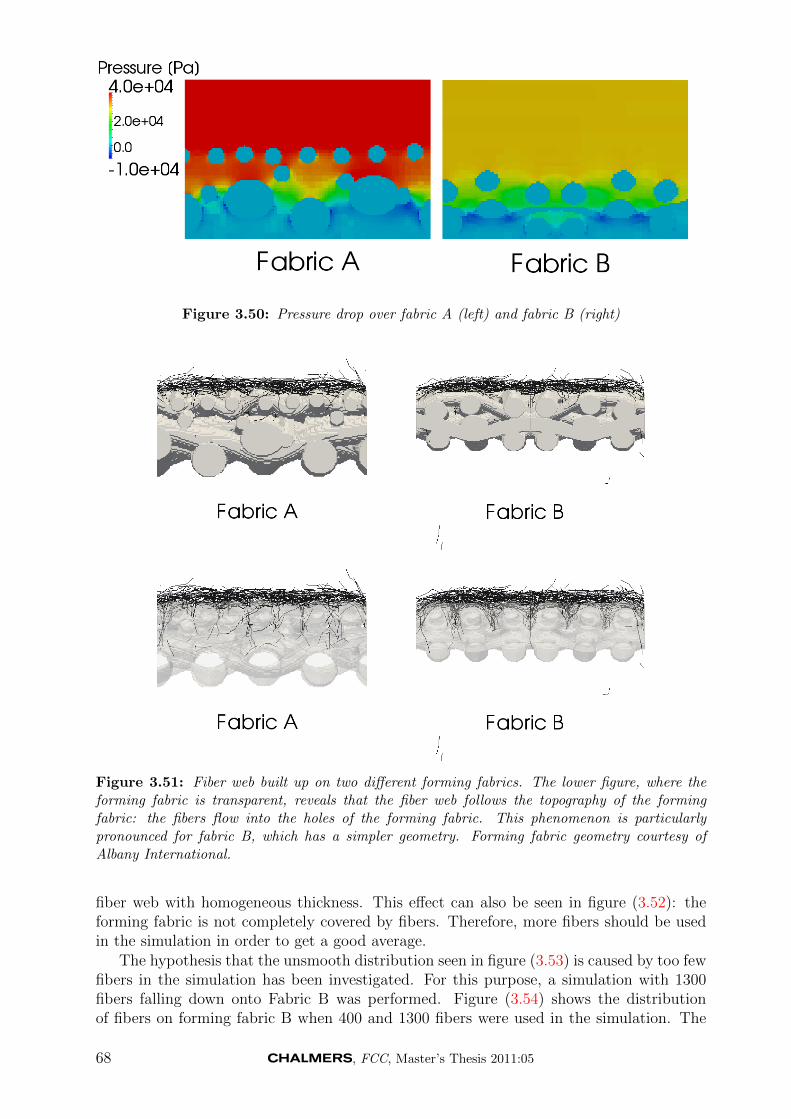
Figure 3.50: Pressure drop over fabric A (left) and fabric B (right)

Figure 3.51: Fiber web built up on two different forming fabrics. The lower figure, where theforming fabric is transparent, reveals that the fiber web follows the topography of the formingfabric: the fibers flow into the holes of the forming fabric. This phenomenon is particularlypronounced for fabric B, which has a simpler geometry. Forming fabric geometry courtesy ofAlbany International.

fiber web with homogeneous thickness. This effect can also be seen in figure (3.52): theforming fabric is not completely covered by fibers. Therefore, more fibers should be usedin the simulation in order to get a good average.

The hypothesis that the unsmooth distribution seen in figure (3.53) is caused by too fewfibers in the simulation has been investigated. For this purpose, a simulation with 1300fibers falling down onto Fabric B was performed. Figure (3.54) shows the distributionof fibers on forming fabric B when 400 and 1300 fibers were used in the simulation. The


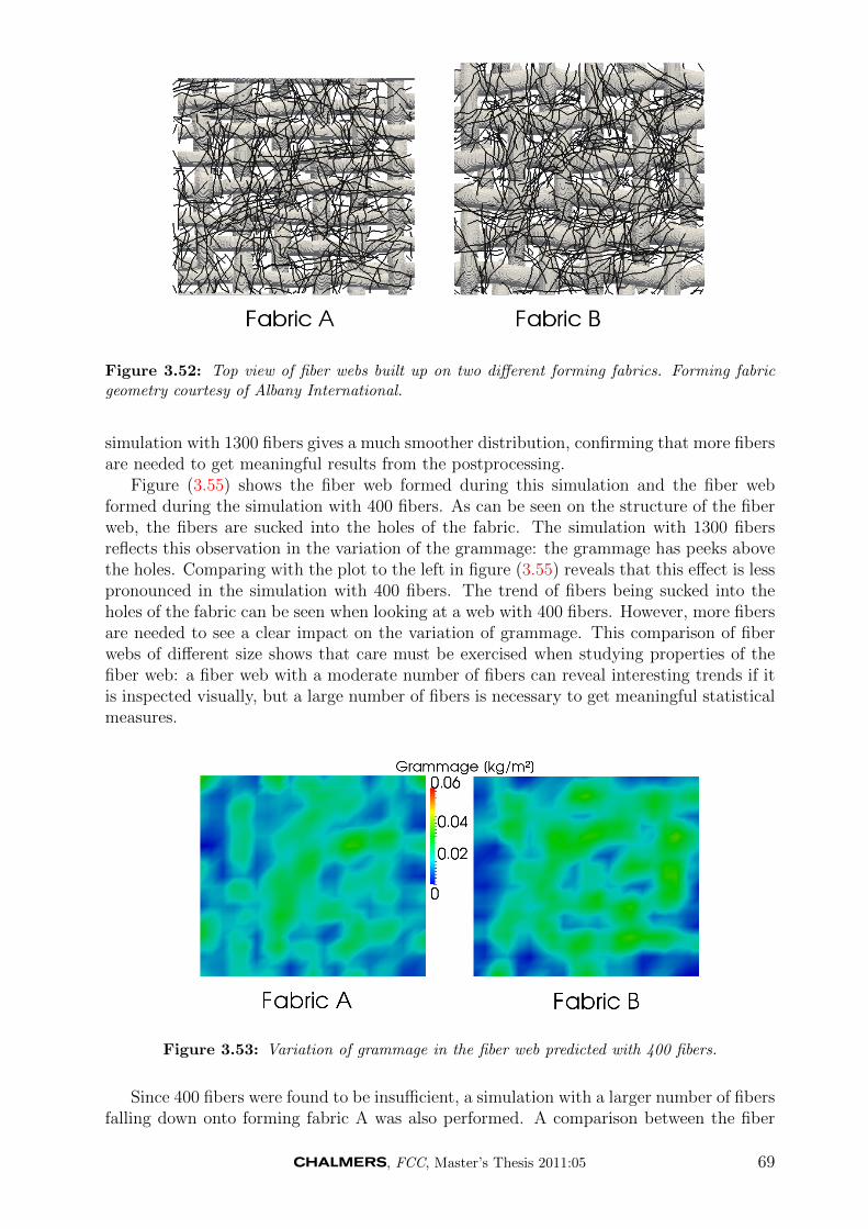
Figure 3.52: Top view of fiber webs built up on two different forming fabrics. Forming fabricgeometry courtesy of Albany International.

simulation with 1300 fibers gives a much smoother distribution, confirming that more fibersare needed to get meaningful results from the postprocessing.

Figure (3.55) shows the fiber web formed during this simulation and the fiber webformed during the simulation with 400 fibers. As can be seen on the structure of the fiberweb, the fibers are sucked into the holes of the fabric. The simulation with 1300 fibersreflects this observation in the variation of the grammage: the grammage has peeks abovethe holes. Comparing with the plot to the left in figure (3.55) reveals that this effect is lesspronounced in the simulation with 400 fibers. The trend of fibers being sucked into theholes of the fabric can be seen when looking at a web with 400 fibers. However, more fibersare needed to see a clear impact on the variation of grammage. This comparison of fiberwebs of different size shows that care must be exercised when studying properties of thefiber web: a fiber web with a moderate number of fibers can reveal interesting trends if itis inspected visually, but a large number of fibers is necessary to get meaningful statisticalmeasures.

Figure 3.53: Variation of grammage in the fiber web predicted with 400 fibers.

Since 400 fibers were found to be insufficient, a simulation with a larger number of fibersfalling down onto forming fabric A was also performed. A comparison between the fiber


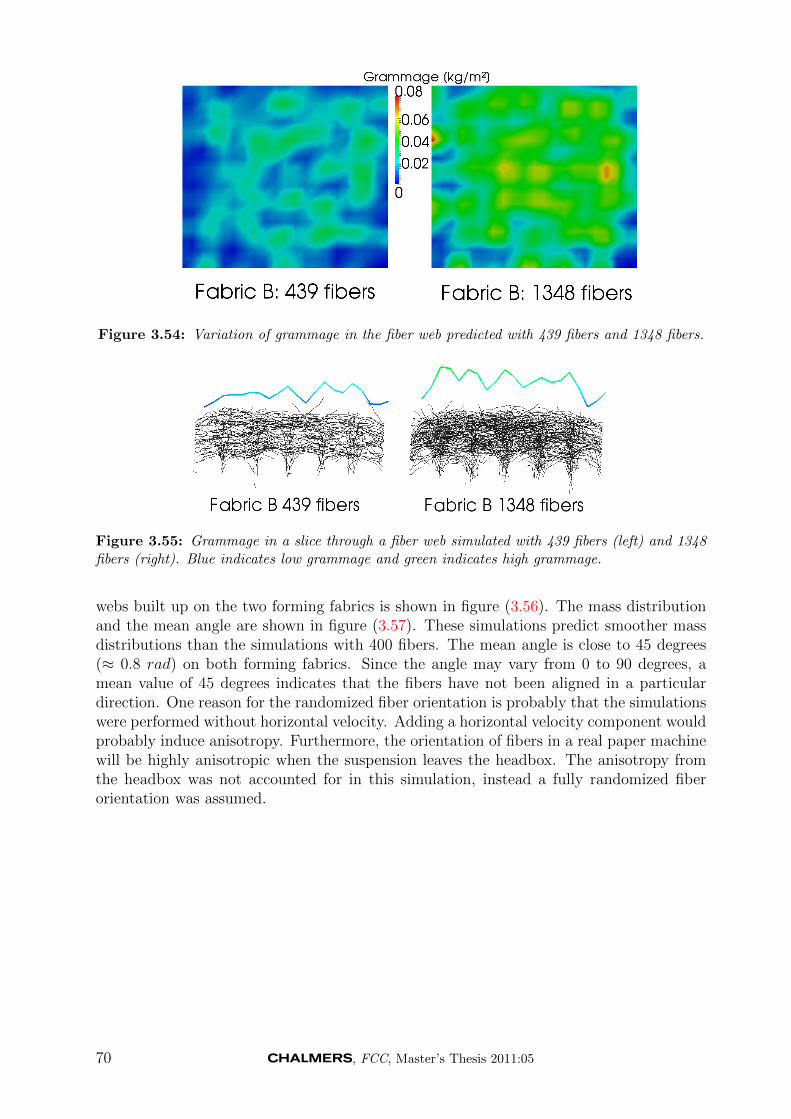
Figure 3.54: Variation of grammage in the fiber web predicted with 439 fibers and 1348 fibers.

Figure 3.55: Grammage in a slice through a fiber web simulated with 439 fibers (left) and 1348fibers (right). Blue indicates low grammage and green indicates high grammage.

webs built up on the two forming fabrics is shown in figure (3.56). The mass distributionand the mean angle are shown in figure (3.57). These simulations predict smoother massdistributions than the simulations with 400 fibers. The mean angle is close to 45 degrees(≈ 0.8 rad) on both forming fabrics. Since the angle may vary from 0 to 90 degrees, amean value of 45 degrees indicates that the fibers have not been aligned in a particulardirection. One reason for the randomized fiber orientation is probably that the simulationswere performed without horizontal velocity. Adding a horizontal velocity component wouldprobably induce anisotropy. Furthermore, the orientation of fibers in a real paper machinewill be highly anisotropic when the suspension leaves the headbox. The anisotropy fromthe headbox was not accounted for in this simulation, instead a fully randomized fiberorientation was assumed.


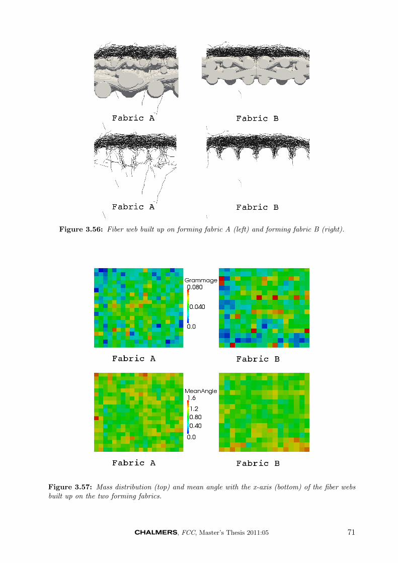
Figure 3.56: Fiber web built up on forming fabric A (left) and forming fabric B (right).

Figure 3.57: Mass distribution (top) and mean angle with the x-axis (bottom) of the fiber websbuilt up on the two forming fabrics.


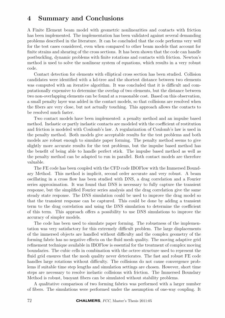
4 Summary and Conclusions

A Finite Element beam model with geometric nonlinearities and contacts with frictionhas been implemented. The implementation has been validated against several demandingproblems described in the literature. It can be concluded that the code performs very wellfor the test cases considered, even when compared to other beam models that account forfinite strains and shearing of the cross sections. It has been shown that the code can handlepostbuckling, dynamic problems with finite rotations and contacts with friction. Newton’smethod is used to solve the nonlinear system of equations, which results in a very robustcode.

Contact detection for elements with elliptical cross section has been studied. Collisioncandidates were identified with a kd-tree and the shortest distance between two elementswas computed with an iterative algorithm. It was concluded that it is difficult and com-putationally expensive to determine the overlap of two elements, but the distance betweentwo non-overlapping elements can be found at a reasonable cost. Based on this observation,a small penalty layer was added in the contact models, so that collisions are resolved whenthe fibers are very close, but not actually touching. This approach allows the contacts tobe resolved much faster.

Two contact models have been implemented: a penalty method and an impulse basedmethod. Inelastic or partly inelastic contacts are modeled with the coefficient of restitutionand friction is modeled with Coulomb’s law. A regularization of Coulomb’s law is used inthe penalty method. Both models give acceptable results for the test problems and bothmodels are robust enough to simulate paper forming. The penalty method seems to giveslightly more accurate results for the test problems, but the impulse based method hasthe benefit of being able to handle perfect stick. The impulse based method as well asthe penalty method can be adapted to run in parallel. Both contact models are thereforevaluable.

The FE code has been coupled with the CFD code IBOFlow with the Immersed Bound-ary Method. This method is implicit, second order accurate and very robust. A beamoscillating in a cross flow has been studied with DNS, a drag correlation and a Fourierseries approximation. It was found that DNS is necessary to fully capture the transientresponse, but the simplified Fourier series analysis and the drag correlation give the samesteady state response. The DNS simulation could be used to improve the drag model sothat the transient response can be captured. This could be done by adding a transientterm to the drag correlation and using the DNS simulation to determine the coefficientof this term. This approach offers a possibility to use DNS simulations to improve theaccuracy of simpler models.

The code has been used to simulate paper forming. The robustness of the implemen-tation was very satisfactory for this extremely difficult problem. The large displacementsof the immersed objects are handled without difficulty and the complex geometry of theforming fabric has no negative effects on the fluid mesh quality. The moving adaptive gridrefinement technique available in IBOFlow is essential for the treatment of complex movingboundaries. The cubic cells in combination with the octree structure used to represent thefluid grid ensures that the mesh quality never deteriorates. The fast and robust FE codehandles large rotations without difficulty. The collisions do not cause convergence prob-lems if suitable time step lengths and simulation settings are chosen. However, short timesteps are necessary to resolve inelastic collisions with friction. The Immersed BoundaryMethod is robust, buoyant fibers can be simulated without stability problems.

A qualitative comparison of two forming fabrics was performed with a larger numberof fibers. The simulations were performed under the assumption of one-way coupling. It


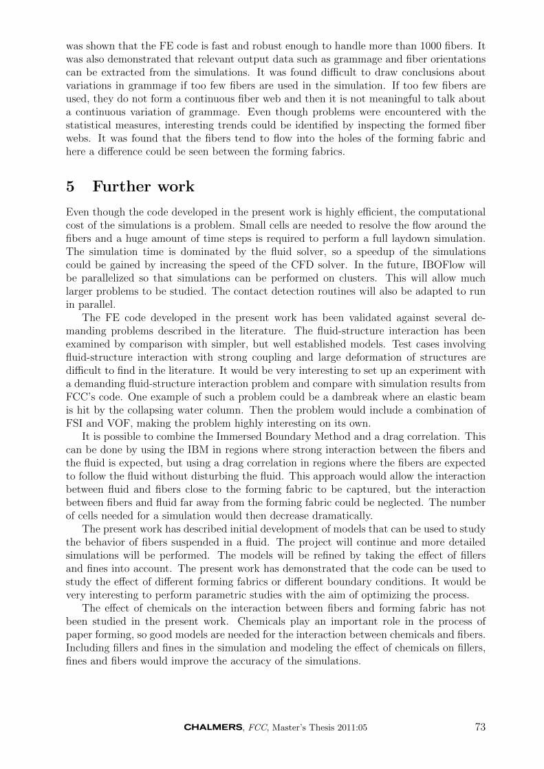
was shown that the FE code is fast and robust enough to handle more than 1000 fibers. Itwas also demonstrated that relevant output data such as grammage and fiber orientationscan be extracted from the simulations. It was found difficult to draw conclusions aboutvariations in grammage if too few fibers are used in the simulation. If too few fibers areused, they do not form a continuous fiber web and then it is not meaningful to talk abouta continuous variation of grammage. Even though problems were encountered with thestatistical measures, interesting trends could be identified by inspecting the formed fiberwebs. It was found that the fibers tend to flow into the holes of the forming fabric andhere a difference could be seen between the forming fabrics.

5 Further work

Even though the code developed in the present work is highly efficient, the computationalcost of the simulations is a problem. Small cells are needed to resolve the flow around thefibers and a huge amount of time steps is required to perform a full laydown simulation.The simulation time is dominated by the fluid solver, so a speedup of the simulationscould be gained by increasing the speed of the CFD solver. In the future, IBOFlow willbe parallelized so that simulations can be performed on clusters. This will allow muchlarger problems to be studied. The contact detection routines will also be adapted to runin parallel.

The FE code developed in the present work has been validated against several de-manding problems described in the literature. The fluid-structure interaction has beenexamined by comparison with simpler, but well established models. Test cases involvingfluid-structure interaction with strong coupling and large deformation of structures aredifficult to find in the literature. It would be very interesting to set up an experiment witha demanding fluid-structure interaction problem and compare with simulation results fromFCC’s code. One example of such a problem could be a dambreak where an elastic beamis hit by the collapsing water column. Then the problem would include a combination ofFSI and VOF, making the problem highly interesting on its own.

It is possible to combine the Immersed Boundary Method and a drag correlation. Thiscan be done by using the IBM in regions where strong interaction between the fibers andthe fluid is expected, but using a drag correlation in regions where the fibers are expectedto follow the fluid without disturbing the fluid. This approach would allow the interactionbetween fluid and fibers close to the forming fabric to be captured, but the interactionbetween fibers and fluid far away from the forming fabric could be neglected. The numberof cells needed for a simulation would then decrease dramatically.

The present work has described initial development of models that can be used to studythe behavior of fibers suspended in a fluid. The project will continue and more detailedsimulations will be performed. The models will be refined by taking the effect of fillersand fines into account. The present work has demonstrated that the code can be used tostudy the effect of different forming fabrics or different boundary conditions. It would bevery interesting to perform parametric studies with the aim of optimizing the process.

The effect of chemicals on the interaction between fibers and forming fabric has notbeen studied in the present work. Chemicals play an important role in the process ofpaper forming, so good models are needed for the interaction between chemicals and fibers.Including fillers and fines in the simulation and modeling the effect of chemicals on fillers,fines and fibers would improve the accuracy of the simulations.


References

[1] A. Bostrom. Fundamental structural dynamics. Department of Mechanics, ChalmersUniversity of Technology, 2001.

[2] A. Chatterjee and A. Ruina. A new algebraic rigid body collision law based on impulsespace considerations. Journal of Applied Mechanics, 65:939–951, 1998.

[3] A. B. Chaudhary and K. J. Bathe. A solution method for static and dynamic analysisof three-dimensional contact problems with friction. Computers and Structures, 6:855–873, 1986.

[4] F. Cirak and M. West. Decomposition contact response (dcr) for explicit finite elementdynamics. International Journal for Numerical Methods in Engineering, 64:1078–1110,2005.

[5] M.A. Crisfield, U. Galvanetto, and G. Jelenic. Dynamics of 3-d co-rotational beams.Computational Mechanics, 20:507–519, 1997.

[6] C. Crowe, M. Sommerfeld, and Y. Tsuji. Multiphase flows with droplets and particles.CRC Press, 1998.

[7] H. M. de la Fuente and C.A. Felippa. Ephemeral penalty functions for contact-impactdynamics. Finite Elements in Analysis and Design, 9:177–191, 1991.

[8] G. Dhondt and K. Wittig. Calculix, a free software three-dimensional structural finiteelement program. http://www.Calculix.de.

[9] J.H. Argyris et al. Finite element method - the natural approach. Comput. Methodsin Appl. Mech. Engrg., 17/18:1–106, 1979.

[10] GeoDict. http://www.geodict.com.

[11] F. Gruttmann, R. Sauer, and W. Wagner. A geometrical nonlinear eccentric 3d-beam element with arbitrary cross-sections. Comput. Methods in Appl. Mech. Engrg.,160:383–400, 1998.

[12] S. M. Han, H. Benaroya, and T. Wei. Dynamics of transversely vibrating beams usingfour engineering theories. Journal of Sound and Vibration, 225:935–988, 1999.

[13] D. Harmon. Robust, Efficient and Accurate Contact Algorithms. PhD thesis, Columbiauniversity, 2010.

[14] H. M. Hilber, T. J. R. Hughes, and R. L. Taylor. Improved numerical dissipationfor time integration algorithms in structural dynamics. Earthquake Engineering andStructural Dynamics, 5:283–292, 1977.

[15] T. J. R. Hughes. The Finite Element Method - Linear Static and Dynamic FiniteElement Analysis. Dover, New York, 1987.

[16] IBOFlow. http://www.fcc.chalmers.se/comp/products/iboflow/.

[17] A. Ibrahimbegovic and M.A. Mikdad. Finite rotations in dynamics of beams andimplicit time-stepping schemes. International Journal for Numerical Methods in En-gineering, 41:781–814, 1998.


http://www.Calculix.de

http://www.geodict.com

http://www.fcc.chalmers.se/comp/products/iboflow/

[18] S. B. Lindstrom and T. Uesaka. Simulation of the motion of flexible fibers in viscousfluid flow. Physics of Fluids, 19:113307, 2007.

[19] S. B. Lindstrom and T. Uesaka. Particle-level simulation of forming of the fibernetwork in papermaking. International Journal of Engineering Science, 46:858–876,2008.

[20] S. B. Lindstrom and T. Uesaka. Simulation of semidilute suspensions of non-brownianfibers in shear flow. The Journal of Chemical Physics, 128:024901, 2008.

[21] A. Mark. The Mirroring Immersed Boundary Method - Modeling Fluids with Movingand Interacting Bodies. PhD thesis, Chalmers University of Technology, 2008.

[22] A. Mark, R. Rundqvist, and F. Edelvik. Comparison between different immersedboundary conditions for simulation of complex fluid flows. International Conferenceon Multiphase Flow, 2010.

[23] E. E. Michaelides. Particles, bubbles and drops. World Scientific Publishing, 2006.ISBN: 981-256-647-3.

[24] B. Nour-Omid and C.C. Rankin. The use of projectors to improve finite elementperformance. Computers and Structures, 30:257–267, 1988.

[25] B. Nour-Omid and C.C. Rankin. Finite rotation analysis and consistent linearizationusing projectors. Computer Methods in Applied Mechanics and Engineering, 93:353–384, 1991.

[26] N. Ottosen and H. Peterson. Introduction to the Finite Element Method. PrenticeHall, 1992.

[27] M. J. D. Powell. An efficient method for finding the minimum of a function of severalvariables without calculating derivatives. The Computer Journal, 7:155–162, 1964.

[28] J.C. Simo and L. Vu-Quoc. A three-dimensional finite-strain rod model. part ii: Com-putational aspects. Computer Methods in Applied Mechanics and Engineering, 58:79–116, 1986.

[29] J.C. Simo and L. Vu-Quoc. On the dynamics in space of rods undergoing largemotions - a geometrically exact approach. Computer Methods in Applied Mechanicsand Engineering, 66:125–161, 1988.

[30] D.E. Stewart and J.C. Trinkle. An implicit time-stepping scheme for rigid bodydynamics with inelastic collisions and coulomb friction. International Journal forNumerical Methods in Engineering, 39:2673–2691, 1996.

[31] J.R. Williams and R. O’Connor. Discrete element simulation and the contact problem.Archives of Computational Methods in Engineering, 6:279–304, 1999.

[32] P. Wriggers. Computational Contact Mechanics. Springer Berlin Heidelberg NewYork, 2006.


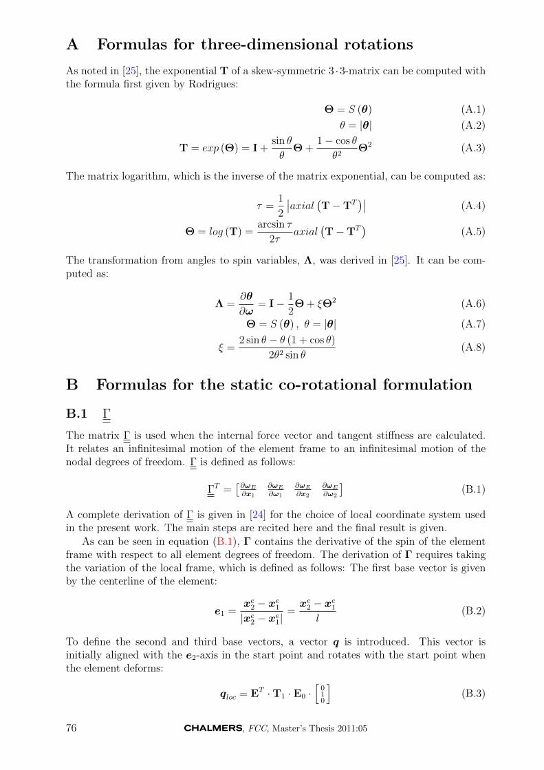
A Formulas for three-dimensional rotations

As noted in [25], the exponential T of a skew-symmetric 3 ·3-matrix can be computed withthe formula first given by Rodrigues:

Θ = S (θ) (A.1)

θ = |θ| (A.2)

T = exp (Θ) = I +sin θ

θΘ +

1− cos θ

θ2Θ2 (A.3)

The matrix logarithm, which is the inverse of the matrix exponential, can be computed as:

τ =1

2

∣∣axial (T−TT)∣∣ (A.4)

Θ = log (T) =arcsin τ

2τaxial

(T−TT

)(A.5)

The transformation from angles to spin variables, Λ, was derived in [25]. It can be com-puted as:

Λ =∂θ

∂ω= I− 1

2Θ + ξΘ2 (A.6)

Θ = S (θ) , θ = |θ| (A.7)

ξ =2 sin θ − θ (1 + cos θ)

2θ2 sin θ(A.8)

B Formulas for the static co-rotational formulation

B.1 Γ

The matrix Γ is used when the internal force vector and tangent stiffness are calculated.It relates an infinitesimal motion of the element frame to an infinitesimal motion of thenodal degrees of freedom. Γ is defined as follows:

ΓT =[∂ωE∂x1

∂ωE∂ω1

∂ωE∂x2

∂ωE∂ω2

](B.1)

A complete derivation of Γ is given in [24] for the choice of local coordinate system usedin the present work. The main steps are recited here and the final result is given.

As can be seen in equation (B.1), Γ contains the derivative of the spin of the elementframe with respect to all element degrees of freedom. The derivation of Γ requires takingthe variation of the local frame, which is defined as follows: The first base vector is givenby the centerline of the element:

e1 =xe2 − xe1|xe2 − xe1|

=xe2 − xe1

l(B.2)

To define the second and third base vectors, a vector q is introduced. This vector isinitially aligned with the e2-axis in the start point and rotates with the start point whenthe element deforms:

qloc = ET ·T1 · E0 ·[

010

](B.3)


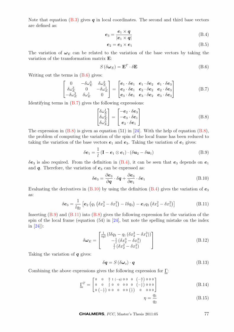
Note that equation (B.3) gives q in local coordinates. The second and third base vectorsare defined as:

e3 =e1 × q|e1 × q|

(B.4)

e2 = e3 × e1 (B.5)

The variation of ωE can be related to the variation of the base vectors by taking thevariation of the transformation matrix E:

S (δωE) = ET · δE (B.6)

Writing out the terms in (B.6) gives: 0 −δω3E δω2

E

δω3E 0 −δω1

E

−δω2E δω1

E 0

=

e1 · δe1 e1 · δe2 e1 · δe3

e2 · δe1 e2 · δe2 e2 · δe3

e3 · δe1 e3 · δe2 e3 · δe3

(B.7)

Identifying terms in (B.7) gives the following expressions:δω1E

δω2E

δω3E

=

−e2 · δe3

−e3 · δe1

e2 · δe1

(B.8)

The expression in (B.8) is given as equation (51) in [24]. With the help of equation (B.8),the problem of computing the variation of the spin of the local frame has been reduced totaking the variation of the base vectors e1 and e3. Taking the variation of e1 gives:

δe1 =1

l(I− e1 ⊗ e1) · (δu2 − δu1) (B.9)

δe3 is also required. From the definition in (B.4), it can be seen that e3 depends on e1

and q. Therefore, the variation of e3 can be expressed as:

δe3 =∂e3

∂q· δq +

∂e3

∂e1

· δe1 (B.10)

Evaluating the derivatives in (B.10) by using the definition (B.4) gives the variation of e3

as:

δe3 =1

lq2

[e2

(q1

(δx3

2 − δx31

)− lδq3

)− e1q2

(δx2

2 − δx21

)](B.11)

Inserting (B.9) and (B.11) into (B.8) gives the following expression for the variation of thespin of the local frame (equation (54) in [24], but note the spelling mistake on the indexin [24]):

δωE =

1lq2

(lδq3 − q1 (δx32 − δx3

1))

−1l

(δx32 − δx3

1)1l

(δx22 − δx2

1)

(B.12)

Taking the variation of q gives:

δq = S (δωs) · q (B.13)

Combining the above expressions gives the following expression for Γ:

ΓT =

[0 0 η

l1 (−η) 0 0 0 (− ηl ) 0 0 0

0 0 1l

0 0 0 0 0 (− 1l ) 0 0 0

0 (− 1l ) 0 0 0 0 0 ( 1

l ) 0 0 0 0

](B.14)

η =q1

q2

(B.15)


B.2 P

According to eqn (33) in [25], the 6 · 6 blocks of the matrix P can be computed as:

Pab

= Iδab −Ψa· ΓT

b(B.16)

By taking Γ from (B.14) and Ψ from equation (34) in [25], the projector matrix P is foundto be:

P =

1 0 0 0 0 0 0 0 0 0 0 00 1 0 0 0 0 0 0 0 0 0 00 0 1 0 0 0 0 0 0 0 0 00 0 −η/l 0 η 0 0 0 η/l 0 0 00 0 −1/l 0 1 0 0 0 1/l 0 0 00 1/l 0 0 0 1 0 −1/l 0 0 0 00 0 0 0 0 0 1 0 0 0 0 00 1 0 0 0 0 0 0 0 0 0 00 0 1 0 0 0 0 0 0 0 0 00 0 −η/l −1 η 0 0 0 η/l 1 0 00 0 −1/l 0 0 0 0 0 1/l 0 1 00 1/l 0 0 0 0 0 −1/l 0 0 0 1

(B.17)

B.3 F

The matrix F depends on the internal force vector of an element. Let n1 and m1 be theinternal force and moment in the start point of the element. In the same way, let n2 andm2 be the internal force and moment in the end point. The matrix F is defined in [25] as:

F =

S (n1)

12S (m1)

S (n2)

12S (m2)

(B.18)

Here, S () denotes the spin operator described in the theory section.

C Fourier series expansion of an oscillating cantilever

beam in a fluid

The force on a cylinder submerged in a fluid can be described by the drag force. Otherforces, such as the history force, may also be important. However, only the drag force isconsidered in this simplified Fourier series expansion. For a given cylinder geometry, thedrag coefficient cd can be obtained from tabulated data or curve fitting formulas and thetotal drag force on the cylinder is computed as [6]:

Fdrag =1

2ρF cdAproj

∣∣∣uF − ·w∣∣∣ (uF − ·

w)

(C.1)

In the present work, values for cd for flow around a long cylinder given by Clift et al. areused [23]:

cd = 9.689Re0.78

(1 + 0.147 ·Re0.82) if 0.1 < Re < 5

cd = 9.689Re0.78

(1 + 0.227 ·Re0.5) if 5 ≤ Re < 40

cd = 9.689Re0.78

(1 + 0.0838 ·Re0.82) if 40 ≤ Re < 400

(C.2)


The projected area of a circular beam is Aproj = 2r · L, where r is the radius of the beamand L is the total beam length. The force per unit length on a thin slice of the beam istherefore:

q =1

2ρF cd2r

∣∣∣vF − ·w∣∣∣ (vF − ·

w)

(C.3)

With the fluid properties and simulation settings used here, the boundary layer on thelower wall will be thin compared to the length of the beam. Therefore, the far-field fluidvelocity is regarded as constant. As a result, the fluid force on the beam will only varywith the beam velocity in that point.

The Euler-Bernoulli beam equation can be written as [1]:

α··w =

q

EI− wIV , α =

AcsρsEI

(C.4)

Here, a superscript with roman letters denotes derivative with respect to x, the coordinatein the axial direction of the beam. Acs is the cross section area of the beam and w denotesthe deflection of the beam. The problem can be studied with modal analysis by makingthe following ansatz for the deflection:

w (x, t) ≈m∑n=1

Xn (x)Tn (t) (C.5)

In the equation above, Xn is a function of x only and Tn is a function of t only. Subscriptn denotes functions associated with mode n and m is the total number of modes includedin the approximation. The functions Xn must fulfill the boundary conditions. For Euler-Bernoulli beams, Xn can be expressed in Duncan functions [1]:

Xn = A1ns1 (µnx) + A2nc1 (µnx) + A3ns2 (µnx) + A4nc2 (µnx) (C.6)

s1 (ξ) = sin ξ + sinh ξ (C.7)

c1 (ξ) = cos ξ + cosh ξ (C.8)

s2 (ξ) = − sin ξ + sinh ξ (C.9)

c2 (ξ) = − cos ξ + cosh ξ (C.10)

As noted in [1], the Duncan functions are related through:

c2 (ξ) = s′

2 (ξ) = c′′

1 (ξ) = s′′′

1 (ξ) (C.11)

Furthermore, the Duncan functions are ideal for Dirichlet boundary conditions at ξ = 0because they have the following convenient properties [1]:

s1 (0) = s2 (0) = c2 (0) = 0, c1 (0) = 2 (C.12)

c′

1 (0) = s′

2 (0) = c′

2 (0) = 0, s′

1 (0) = 2 (C.13)

s′′

1 (0) = c′′

1 (0) = s′′

2 (0) = 0, c′′

2 (0) = 2 (C.14)

s′′′

1 (0) = c′′′

1 (0) = c′′′

2 (0) = 0, s′′′

2 (0) = 2 (C.15)

The beam studied in this example is clamped at the left end and free at the right end.Therefore, the deflection and the angle are zero at x = 0. The bending moment and thetransverse force are zero at the free end at x = L. These boundary conditions must be


fulfilled at all instants in time and therefore Xn must fulfill these conditions. The resultingconditions on Xn are:

Xn (0) = 0 (C.16)

X′

n (0) = 0 (C.17)

X′′

n (λnL) = 0 (C.18)

X′′′

n (λnL) = 0 (C.19)

By inserting these conditions into (C.6), the eigenvalue λn and three of the constantsA1n, A2n, A3n and A4n can be obtained. The result is the following expression for Xn:

Xn (x) = A4n

[c2 (λnx)− c1 (λnL)

s1 (λnL)s2 (λnx)

](C.20)

If the constant A4n is included in the time function Tn (t), the deflection can be expressedas:

w (x, t) =∞∑n=1

Tn (t)

[c2 (λnx)− c1 (λnL)

s1 (λnL)s2 (λnx)

](C.21)

Insert (C.21) into the PDE in (C.4):

∞∑n=1

Tn (t)λ4n

[s1 (λnx)− c1 (λnL)

s1 (λnL)c2 (λnx)

]= (C.22)

=∞∑n=1

(−Acsρs

EI

··T n (t)

[s1 (λnx)− c1 (λnL)

s1 (λnL)c2 (λnx)

])+

q

EI(C.23)

Define ω2n = λ4

nEIAρs

and bn = c1(λnL)s1(λnL)

. Insert these definitions together with the expression

for the distributed load in equation (C.23):

∞∑n=1

[ω2nTn +

··T n

][s1 (λnx)− bnc2 (λnx)] = − q0

Acsρs

∣∣∣ ·wrel∣∣∣ ·wrel (C.24)

Expand the load in the same Fourier series as X (x):

f = − q0

Aρs

∣∣∣ ·w − vf ∣∣∣ ( ·w − vf) !=∞∑n=1

an (t) [c2 (λnx)− bns2 (λnx)] (C.25)

To compute the coefficients an, start by multiplying (C.25) by the eigenmode shape[c2 (λmx)− bns2 (λmx)] and integrate over the length of the beam:∫ L

0

f · [c2 (λmx)− bns2 (λmx)] dx =

∫ L

0

∞∑n=1

an (t) [c2 (λnx)− bns2 (λnx)] [c2 (λmx)− bms2 (λmx)] dx =

=∞∑n=1

an (t)

∫ L

0

[c2 (λnx)− bns2 (λnx)] [c2 (λmx)− bms2 (λmx)] dx︸︷︷︸I1

(C.26)

The integral I1 in equation (C.26) was evaluated numerically. It was found that the or-thogonality of the eigenmodes holds and the value of the integral was found to be:

I1 =

∫ L

0

[c2 (λnx)− bns2 (λnx)] [c2 (λmx)− bms2 (λmx)] dx = L · δmn (C.27)


Here δmn denotes the Kronecker delta. Inserting (C.27) in (C.26) gives an as:

an (t) =1

L

∫ L

0

f · [c2 (λnx)− bns2 (λnx)] dx =

=1

L

∫ L

0

q0

Aρs

∣∣∣ ·w − vf ∣∣∣ ( ·w − vf) [c2 (λnx)− bns2 (λnx)] dx (C.28)

The integral in equation (C.28) above is a complicated function of x and would be difficultto integrate analytically. Especially, note that q0 depends on cd which in turn is a functionof the Reynolds number Re. The Reynolds number is calculated from the local relativevelocity, which varies with x, so that q0 = q0 (x). Therefore, the integral in (C.28) isintegrated numerically with the Runge-Kutta 45 scheme. When an has been evaluated,the expanded expression for the load can be inserted in equation (C.24):

∞∑n=1

[··T n + ω2

nTn

][c2 (λnx)− bns2 (λnx)] =

∞∑n=1

an (t) [c2 (λnx)− bns2 (λnx)] (C.29)

Equation (C.29) gives an ordinary differential equation for each Tn:

··T n + ω2

nTn = an (C.30)

Equation (C.30) can be integrated in time with Newmark’s method. Let k denote timestep. The acceleration at the new time step is computed as:

··Tk+1

n =1

β∆t2

[(T k+1n − T kn

)−∆t

·Tk

n −∆t2 (0.5− β)··Tk

n

](C.31)

Insert (C.31) in (C.30):

1

β∆t2T k+1n +

1

β∆t2

[−T kn −∆t

·Tk

n −∆t2 (0.5− β)··Tk

n

]︸︷︷︸

ck

+ω2nT

k+1n = ak+1

n (C.32)

If semi-explicit integration is used, so that an is evaluated at the previous time step insteadof at the current time step, T k+1

n can be computed as:

T k+1n =

akn − ck(1

β∆t2+ ω2

n

) (C.33)

When T k+1n is known the velocity and acceleration are updated according to:

·Tk+1

n =γ

β∆t

(T k+1n − T kn

)+

(1− γ

β

)·Tk

n + ∆t

(1− γ

2β

)··Tk

n (C.34)

··Tk+1

n =1

β∆t2

[(T k+1n − T kn

)−∆t

·Tk

n −∆t2 (0.5− β)··Tk

n

](C.35)

D Jacobian of inertia force

To compute the Jacobian of the inertia force, first consider the variation of the translationalterms:

δ(NaρA

··u)

= NaρAδ··u = NaρA

∂··u

∂u· δu (D.1)


The derivative of the nodal acceleration with respect to the nodal displacement must bedetermined to evaluate the expression above. In the present work, Newmark’s interpolationis used to interpolate the nodal quantities in time. In the following, β and γ denote theNewmark interpolation parameters. The relation between the coordinate and accelerationat the new time step is given by equation (53) in [5]:

··un+1

=1

β∆t2

[(un+1 − un

)−∆t

·un−∆t2 (0.5− β)

··un]

(D.2)

Take the derivative of (D.2):

∂··un+1

i

∂un+1j

=δijβ∆t2

(D.3)

Insert (D.3) and (2.60) in (2.59):

δ(NaρA

··u)

=NaρA

β∆t2δu =

NaN1ρA

β∆t2δu1 +

NaN2ρA

β∆t2δu2, a = 1, 2 (D.4)

The formula above gives an explicit expression for the inertia stiffness terms correspondingto the translational degrees of freedom.

Next, consider the variation of the rotational terms, which is more involved. Takingthe variation of the rotational terms in (2.59) gives:

δ[Na

(S (w) · E · J · ET ·w + E · J · ET · ·w

)]=

Na (δS (w)) · E · J · ET ·w︸︷︷︸c1

+NaS (w) · (δE) · J · ET ·w︸︷︷︸c2

+NaS (w) · E · J ·(δET

)·w︸︷︷︸

c3

+

NaS (w) · E · J · ET · δw︸︷︷︸c4

+Na (δE) · J · ET · ·w︸︷︷︸c5

+NaE · J ·(δET

)· ·w︸︷︷︸

c6

+NaE · J · ET · δ ·w︸︷︷︸c7

(D.5)

To evaluate the first term above, first note that δS (w) = S (δw). Then consider theNewmark interpolation for the angular velocity given by eqn (54) in [5]:

wn+1 =γ

β∆t

(Ψn+1 −Ψn

)+

(1− γ

β

)wn + ∆t

(1− γ

2β

)·wn

(D.6)

⇒ ∂wn+1i

∂Ψn+1j

=γ

β∆tδij ⇒ δw =

γ

β∆tδΨ (D.7)

Here Ψ is an additive angle parameter. The relation between this angle and the corre-sponding spin variable is given by:

δΨ = H (∆Ψ) · δω (D.8)

Now use (D.7) and (D.8) to evaluate c1 in (D.5):

c1 = −N iγ

β∆tS(E · J · ETw

)·H · δω (D.9)

To evaluate c2, the variation of the local element frame must be computed. To achievethis, first consider the variation of the local frame contracted with an arbitrary vector z:

δE · z = S (δωgE) · E · z = −S (E · z) · δωgE (D.10)


Now consider the variation of the element frame in global coordinates with respect to thenodal degrees of freedom in global coordinates:

δωgE = E · δωeE = E · ∂ωeE

∂xe· δxe = E · ∂ω

eE

∂xe·GT · δxg, (D.11)

G =

[E 0 0 00 E 0 00 0 E 00 0 0 E

], (D.12)

δxg = [δus δωs δue δωe] (D.13)

By comparing (D.11) with [24] and [25], it is noted that:

∂ωeE∂xe

= Γ (D.14)

By using the explicit expression for Γ for a beam given in [24], δωgE can be expressed inknown quantities:

δωgE = E · Γ ·GT︸︷︷︸Γg

·δxg (D.15)

Inserting (D.15) in (D.10) gives the variation of the local frame contracted with a vectorz:

δE · z = −S (E · z) · Γg · δxg (D.16)

Use the expression above to evaluate c2:

c2 = NiS (w) · (δE) · J · ET ·w︸︷︷︸z

= −NiS (w) · S(E · J · ET ·w

)· Γg · δxg (D.17)

To evaluate c3, first consider the variation of the transpose of the local frame contractedwith an arbitrary vector z:(

δET)· z = (S (δωgE) · E)T · z = ET · S (δωgE)T · z =

−ET · S (δωgE) · z = ET · S (z) · δωgE = ET · S (z) · Γg · δxg (D.18)

Inserting (D.18) into the expression for c3 gives:

c3 = NiS (w) · E · J · ET · S (w) · Γg · δxg (D.19)

c4, c5 and c6 can be evaluated in the same way:

c4 = NiS (w) · E · J · ET · δw =Niγ

β∆tS (w) · E · J · ET ·H · δω (D.20)

c5 = Ni (δE) · J · ET · ·w = −NiS(E · J · ET · ·w

)· Γg · δxg (D.21)

c6 = NiE · J ·(δET

)· ·w = NiE · J · ET · S

·(w) · Γg · δxg (D.22)

To evaluate c7, the derivative of the angular acceleration with respect to the nodal degrees offreedom must be computed. This can be done by starting with the Newmark interpolationgiven by equation (55) in [5]:

·wn+1 =

1

β∆t2

(Ψn+1 −Ψn −∆twn −∆t2

(1

2− β

)·wn

)⇒ ∂

·wn+1

∂Ψn+1

=1

β∆t2δij (D.23)

⇒ δ·w =

1

β∆t2δΨ (D.24)


Insert (D.24) into the expression for c7:

c7 =Ni

β∆t2E · J · ET · δΨ =

Ni

β∆t2E · J · ET ·H · δω (D.25)

By inserting the above expressions into (D.5), the contribution to the tangent stiffnessfrom the rotational inertia is obtained.

E Shortest unsigned distance between two segments

Consider a point pI on the surface of segment I and a point pII on the surface of segmentII. Expressed in the local frame of the corresponding element, the coordinates of thesepoints are:

plocI = LIsI , (Rae,IsI +Ras,I(1− sI)) cos(tI), (Rbe,IsI +Rbs,I(1− sI)) sin(tI)plocII = LIIsII , (Rae,IIsII +Ras,II(1− sII)) cos(tII), (Rbe,IIsII +Rbs,II(1− sII)) sin(tII)

(E.1)

Let pIs and pIIs be the start point of segment I and II, respectively. Then, the coordinatesof the surface points can be expressed in the global frame as:

pgI = EI · plocI + pIs (E.2)

pgII = EII · plocII + pIIs (E.3)

The change of basis matrices EI and EII are not a function of s or t and therefore theyare constants. A vector d from a point on segment I to a point on segment II can becomputed as:

d = pgII − pgI = EII · plocII − EI · plocI + pIIs − pIs (E.4)

The square of the distance between the two points is:

d2 = d · d (E.5)

The distance d has extreme values when the square of the distance d2 has extreme values.d2 has extreme values when the gradient is equal to zero:

∂d2

∂xα= 0, xα = sI , tI , sII , tII (E.6)

The system of equations in (E.6) can be solved with Newton’s method. Recasting theproblem into the framework of Newton’s method, the residual becomes:

res1 =∂d2

∂sI= −2diE

Iij

∂pI,locj

∂sI

res2 =∂d2

∂tI= −2diE

Iij

∂pI,locj

∂tI

res3 =∂d2

∂sII= 2diE

IIij

∂pII,locj

∂sII

res4 =∂d2

∂tII= 2diE

IIij

∂pII,locj

∂tII(E.7)


The Jacobian corresponding to the residual in (E.7) is:

K11 =∂2d2

∂sI∂sI= 2EI

ik

∂pI,lock

∂sIEIij

∂pI,locj

∂sI− 2diE

Iij

∂2pI,locj

∂s2I

K12 =∂2d2

∂tI∂sI= 2EI

ik

∂pI,lock

∂tIEIij

∂pI,locj

∂sI− 2diE

Iij

∂2pI,locj

∂tI∂sI

K13 =∂2d2

∂sII∂sI= −2EII

ik

∂pII,lock

∂sIIEIij

∂pI,locj

∂sI

K14 =∂2d2

∂tII∂sI= −2EII

ik

∂pII,lock

∂tIIEIij

∂pI,locj

∂sIK21 = K12

K22 =∂2d2

∂tI∂tI=

∂2d2

∂tI∂sI= 2EI

ik

∂pI,lock

∂tIEIij

∂pI,locj

∂tI− 2diE

Iij

∂2pI,locj

∂tI∂tI

K23 =∂2d2

∂sII∂tI= −2EII

ik

∂pII,lock

∂sIIEIij

∂pI,locj

∂tI

K24 =∂2d2

∂tII∂tI= −2EII

ik

∂pII,lock

∂tIIEIij

∂pI,locj

∂tIK31 = K13

K32 = K23

K33 =∂2d2

∂sII∂sII= 2EII

ik

∂pII,lock

∂sIIEIIij

∂pII,locj

∂sII+ 2diE

IIij

∂2pII,locj

∂s2II

K34 =∂2d2

∂tII∂sII= 2EII

ik

∂pII,lock

∂tIIEIIij

∂pII,locj

∂sII+ 2diE

IIij

∂2pII,locj

∂tII∂sIIK41 = K14

K42 = K24

K43 = K34

K44 =∂2d2

∂tII∂tII= 2EII

ik

∂pII,lock

∂tIIEIIij

∂pII,locj

∂tII+ 2diE

IIij

∂2pII,locj

∂t2II(E.8)

The derivatives of the surface point coordinates in the local frame (∂pI,lock

∂sIand so on )

are computed in exactly the same way as for the case when the shortest distance betweena segment and a point is sought. Note that pI is independent of sII and tII . In the sameway, pII is independent of sI and tI . With the residual in (E.7) and the Jacobian in (E.8),Newton iterations can be performed to find the closest surface points on two segments. Asfor the case when the distance between a segment and a point is sought, the algorithmmust account for the fact that the segments have finite length, so that only sI ∈ [0, 1] andsII ∈ [0, 1] is allowed. This can be achieved by reducing the Jacobian, thus constrainingthe solution to the closest segment edge:

• if sI < 0, then set sI = 0 and reduce the Jacobian and residual according to:

1. res1 = 0

2. K11 = 1

3. K12 = K13 = K14 = K21 = K31 = K41 = 0

• if sI > 1, then set sI = 1 and reduce the Jacobian and residual according to:


1. res1 = 0

2. K11 = 1

3. K12 = K13 = K14 = K21 = K31 = K41 = 0

• if sII < 0, then set sII = 0 and reduce the Jacobian and residual according to:

1. res3 = 0

2. K33 = 1

3. K31 = K32 = K34 = K13 = K23 = K43 = 0

• if sII > 1, then set sII = 1 and reduce the Jacobian and residual according to:

1. res3 = 0

2. K33 = 1

3. K31 = K32 = K34 = K13 = K23 = K43 = 0

The procedure outlined above can be used to find the shortest unsigned distance betweentwo segments. It can, however, not be used to determine the overlap (signed distance)in the case of overlapping segments. If the segments are overlapping, the algorithm willreturn the shortest unsigned distance, which is zero. This fact must be taken into accountin the contact algorithm, e.g. by employing a penalty layer so that overlap never occurs.If the overlap must be computed, a possible solution is to start with the algorithm aboveand first locate the values of s and t corresponding to zero distance. When the Newtoniterations get stuck on this point, one can proceed with an optimization algorithm thatis not based on derivatives, e.g. Powell’s method [27]. The s and t found with Newton’smethod could then be used as initial guess for Powell’s method.


Documents

DevelopmentofanonlinearFiniteElementbeam model for dynamic ...publications.lib.chalmers.se/records/fulltext/142971.pdf · The ber model, which is based on a dynamic co-rotational