Developmentandapplicationsofagrowthmodelfor Pinus radiata ... · AgrowthmodelforradiatapineplantationsinElBierzo 67 beroftreesperhectareandstandbasalarea)areneeded todefinethestandconditionsatanypointintime.To

Instituto Nacional de Investigación y Tecnología Agraria y Alimentación (INIA) Investigación Agraria: Sistemas y Recursos Forestales 2009 18(1), 64-80Disponible on line en www.inia.es/srf ISSN: 1131-7965

Development and applications of a growth model for Pinus radiataD. Don plantations in El Bierzo (Spain)

E. Sevillano-Marco*, A. Fernández-Manso and F. Castedo-DoradoDepartamento de Ingeniería y Ciencias Agrarias, Universidad de León, Escuela Superior y Técnica de Ingeniería Agraria,

Avda. de Astorga SN, 24400 Ponferrada, Spain.

Abstract

A dynamic growth model for Pinus radiata D. Don plantations in El Bierzo (Spain) was developed with data from two inven-tories of permanent plots, of between 7 and 36 years old, established by the University of León. In this model, stand conditions atany point in time are defined by three state variables (stand basal area, number of trees per hectare and dominant height). The modelincludes three transition functions derived by the generalized algebraic difference approach to enable projection of the state vari-ables at any particular time. Once they are known, the number of trees in each diameter class is estimated with a distribution func-tion, by recovery of the parameters of the Weibull function by use of the moments method. Finally, a generalized height-diameterfunction and a taper function allow estimation of total or merchantable stand volume. The model provides satisfactory predictionsfor a time interval of three years. Simulation of the growth of four stands under two silvicultural regimes and two different sitesconfirm that the estimates provided by the overall model adequately represent the effects of both stand density and site quality.Other applications for the model are analysed and discussed.

Key words: forest growth modelling, whole-stand model, disaggregation system, radiata pine, silvicultural alternatives.

Resumen

Desarrollo y aplicaciones de un modelo de crecimiento para plantaciones de Pinus radiata D. Don en El Bierzo (León)

Se ha desarrollado un modelo dinámico de crecimiento para plantaciones de Pinus radiata D. Don en El Bierzo (León) a par-tir de datos de dos inventarios de parcelas permanentes, de entre 7 y 36 años de edad, establecidas por la Universidad de León. Eneste modelo, las condiciones del rodal en un instante dado están definidas por tres variables de estado (área basimétrica, númerode pies por hectárea y altura dominante). El modelo incluye tres funciones de transición obtenidas mediante la metodología deecuaciones en diferencias algebraicas generalizadas que permite la proyección de las variables de estado a un determinado instan-te en el tiempo. Una vez conocidas las variables de estado, una función de distribución estima el número de pies en cada clase dia-métrica mediante la metodología de recuperación de los parámetros de la función de Weibull usando el método de los momentos.Finalmente, una función de altura-diámetro generalizada y una función de perfil de tronco permiten la estimación del volumentotal o comercial del rodal. El modelo proporciona predicciones satisfactorias para un intervalo de proyección de tres años. Lasimulación del crecimiento de cuatro rodales bajo dos regímenes selvícolas distintos y dos calidades de estación diferentes corro-bora que las estimaciones proporcionadas por el modelo global representan adecuadamente los efectos de la densidad de la masay la calidad de la estación. Finalmente se analizan y discuten otras aplicaciones del modelo elaborado.

Palabras clave: modelización del crecimiento forestal, modelo de masa, sistema de desagregación, pino radiata, alternativasselvícolas.

1. Introduction

1.1. Radiata pine in the area of study

Radiata pine (Pinus radiata D. Don) is an exoticspecies introduced in plantations worldwide because of

its high growth rate and all-around advantages (e.g.,Sutton, 1999). It is a well represented species in north-ern Spain, particularly in the Basque Country (160 000ha) and Galicia (92 000 ha).Although radiata pine was introduced in the region of

El Bierzo relatively recently, it currently occupies an

* Corresponding author: [email protected]: 25-08-08. Accepted: 07-01-09.

A growth model for radiata pine plantations in El Bierzo 65

area of approximately 15 000 ha (Fernández-Manso etal., 2001). The oldest stands in the region were plantedin the 1970s, with seeds initially obtained from nearbyareas, such as Galicia. These stands were originally des-tined for production of mining timber, and were there-fore planted at high densities and managed in short rota-tions (approximately 15 years); silvicultural practiceswere rarely carried out. Mining activities have nowdeclined and trends are changing towards extended rota-tions and enhancement of silviculture practices. Theseafforestations introduced the species for the first time ina typical inland region of Spain, where Mediterraneanand Eurosiberian conditions meet.Most of the region is a rural marginal area in which

forestry is becoming a highly recommended type of landuse. Radiata plantations would certainly help to meet thechallenges threatening the area (land abandonment, minerestructuring, decline of traditional economy and of popu-lation), thus contributing to sustainable development.

1.2. Forest growth models

Forest management decisions are based on informa-tion about current and likely future forest conditions.Consequently, it is often necessary to predict thechanges in the system with growth and yield models,which estimate forest dynamics over time. Such modelshave been widely used in forest management becausethey enable updating of inventories, prediction of futureyields, and exploration of management alternatives,thus providing information for decision-making in sus-tainable forest management (Vanclay, 1994).The wide range of forest growth models available dif-

fer in complexity and the detail in which they describethe systems under consideration. At one end of therange are the traditional empirical models based onperiodic tree measurements, which make no attempt tomeasure all factors that may affect tree growth, and atthe other end the complex process models, based on themechanisms inherent to growth, which incorporate alarge amount of information in the response functions.Of the two basic types of empirical models (whole-

stand and individual-tree models), whole-stand modelsare generally recommended when dealing with homoge-neous, even-aged, pure stands (García, 1988, 1993; Van-clay, 1994), because they can be constructed on thebasis of variables often available in forest inventorydata, and also represent a good compromise betweengenerality and accuracy of the estimates.

Whole-stand models characterize the state of thestand by means of a small number of aggregate vari-ables, such as basal area, mean diameter, volume perhectare, stems per hectare, average spacing or top height(García, 1993). This type of models therefore requirefew details for growth simulation. On the other hand,they provide rather limited information about the futurestand (in some cases only stand volume) (Vanclay,1994). To overcome underlying limitations, whole-standmodels can be disaggregated mathematically using adiameter distribution function, which may be combinedwith a generalized height-diameter equation and with ataper function to estimate commercial volumes. Similarmethodologies have been used by Mabvurira et al.(2002), Kotze (2003), Trincado et al. (2003), Diéguez-Aranda et al. (2006a) and Castedo-Dorado et al. (2007)in the development of forest growth models for planta-tions.Preliminary studies in the region of El Bierzo have

provided basic guidelines for the establishment andmanagement of plantations (Castedo-Dorado et al.,2005a). However, the integrity and performance of theseguidelines require a more elaborated simulation tool,such a dynamic growth model.On the other hand, a recently developed whole-stand

model for radiata pine stands is in use in the neighbour-ing region of Galicia (Castedo-Dorado et al., 2007).This model was developed with data from 225 invento-ries of permanent plots and it was demonstrated to berobust for medium term projections of stand volume.Nevertheless, it produces biased estimates when appliedto the local data from the El Bierzo region, as explainedin subsequent sections in this study. For this reason, anattempt was made to localize the already fitted model,so that it can be applied to El Bierzo without the need todevelop a new model. Most adaptation procedures fallinto one of three categories (Huang, 2002): the parame-ter re-estimation method, the proportional adjustmentmethod or the regression adjustment method. Accordingto Huang (2002), the most desirable approach for local-izing any model is to refit the individual components(submodels) with local data. Therefore, the structure ofthe model adopted in this study was the same as thatdescribed by Castedo-Dorado et al. (2007). The samesubmodels were considered (and in most cases the samebase equations), and a new set of parameters were re-estimated from the local data.The objective of the present study was to develop a

management-oriented whole-stand model for simulat-ing the growth of radiata pine plantations in El Bierzo.

66 E. Sevillano-Marco et al. / Invest Agrar: Sist Recur For (2009) 18(1), 64-80

The model is constituted by the same interrelated mod-ules as those developed for the Galician model: a sitequality system (both for dominant height growth andsite index prediction), an equation for reducing treenumber, a stand basal area growth function, and a disag-gregation system composed of a diameter distributionfunction, a generalized height-diameter function and atotal merchantable volume equation.

2. Material and methods

2.1. Data

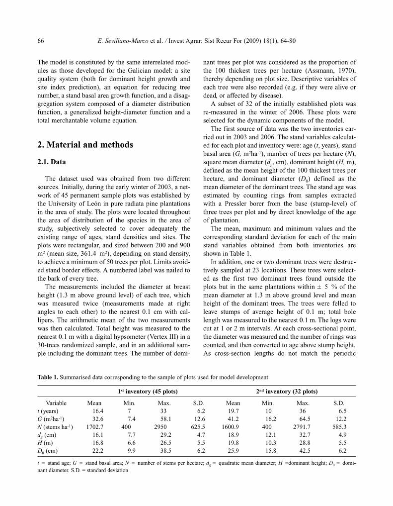
The dataset used was obtained from two differentsources. Initially, during the early winter of 2003, a net-work of 45 permanent sample plots was established bythe University of León in pure radiata pine plantationsin the area of study. The plots were located throughoutthe area of distribution of the species in the area ofstudy, subjectively selected to cover adequately theexisting range of ages, stand densities and sites. Theplots were rectangular, and sized between 200 and 900m2 (mean size, 361.4 m2), depending on stand density,to achieve a minimum of 50 trees per plot. Limits avoid-ed stand border effects. A numbered label was nailed tothe bark of every tree.The measurements included the diameter at breast

height (1.3 m above ground level) of each tree, whichwas measured twice (measurements made at rightangles to each other) to the nearest 0.1 cm with cal-lipers. The arithmetic mean of the two measurementswas then calculated. Total height was measured to thenearest 0.1 m with a digital hypsometer (Vertex III) in a30-trees randomized sample, and in an additional sam-ple including the dominant trees. The number of domi-

nant trees per plot was considered as the proportion ofthe 100 thickest trees per hectare (Assmann, 1970),thereby depending on plot size. Descriptive variables ofeach tree were also recorded (e.g. if they were alive ordead, or affected by disease).A subset of 32 of the initially established plots was

re-measured in the winter of 2006. These plots wereselected for the dynamic components of the model.The first source of data was the two inventories car-

ried out in 2003 and 2006. The stand variables calculat-ed for each plot and inventory were: age (t, years), standbasal area (G, m2ha-1), number of trees per hectare (N),square mean diameter (dg, cm), dominant height (H, m),defined as the mean height of the 100 thickest trees perhectare, and dominant diameter (D0) defined as themean diameter of the dominant trees. The stand age wasestimated by counting rings from samples extractedwith a Pressler borer from the base (stump-level) ofthree trees per plot and by direct knowledge of the ageof plantation.The mean, maximum and minimum values and the

corresponding standard deviation for each of the mainstand variables obtained from both inventories areshown in Table 1.In addition, one or two dominant trees were destruc-

tively sampled at 23 locations. These trees were select-ed as the first two dominant trees found outside theplots but in the same plantations within ± 5 % of themean diameter at 1.3 m above ground level and meanheight of the dominant trees. The trees were felled toleave stumps of average height of 0.1 m; total bolelength was measured to the nearest 0.1 m. The logs werecut at 1 or 2 m intervals. At each cross-sectional point,the diameter was measured and the number of rings wascounted, and then converted to age above stump height.As cross-section lengths do not match the periodic

1st inventory (45 plots) 2nd inventory (32 plots)

Variable Mean Min. Max. S.D. Mean Min. Max. S.D.t (years) 16.4 7 33 6.2 19.7 10 36 6.5G (m2ha-1) 32.6 7.4 58.1 12.6 41.2 16.2 64.5 12.2N (stems ha-1) 1702.7 400 2950 625.5 1600.9 400 2791.7 585.3dg (cm) 16.1 7.7 29.2 4.7 18.9 12.1 32.7 4.9H (m) 16.8 6.6 26.5 5.5 19.8 10.3 28.8 5.5D0 (cm) 22.2 9.9 38.5 6.2 25.9 15.8 42.5 6.2

t = stand age; G = stand basal area; N = number of stems per hectare; dg = quadratic mean diameter; H =dominant height; D0 = domi-nant diameter. S.D. = standard deviation

Table 1. Summarised data corresponding to the sample of plots used for model development


ber of trees per hectare and stand basal area) are neededto define the stand conditions at any point in time. Toproject the future stand state, the model uses three tran-sition functions of the corresponding state variables.Once the state variables are known for a given time, themodel is disaggregated mathematically by use of adiameter distribution function, which is combined witha generalized height-diameter equation and with a taperfunction to estimate total and merchantable stand vol-umes.

2.2.2. Development and fitting of transition functionsfor state variables

Transition functions must possess some importantproperties to provide consistent estimates: (i) consisten-cy, i.e. no change for zero elapsed time; (ii) path-invari-ance, i.e. the result of projecting the state first from t0 tot1, and then from t1 to t2, must be the same as that of theone-step projection from t0 to t2; and (iii) causality, i.e.a change in status can only be influenced by inputs with-in the relevant time interval (García, 1994). Transitionfunctions generated by integration of differential equa-tions (or summation of difference equations when usingdiscrete time) automatically satisfy these conditions.Fulfillment of the above mentioned properties for the

transition functions depends on both the constructionmethod and the mathematical function used to developthe model. Most of these properties can be achievedwith techniques of dynamic equation derivation, knownin forestry as theAlgebraic DifferenceApproach (ADA)(Bailey and Clutter, 1974) or its generalization (GADA)(Cieszewski and Bailey, 2000).Dynamic equations have the general form (omitting

the vector of model parameters) Y = f (t, t0, Y0), where Yis the value of the function at age t, and Y0 is the refer-ence variable defined as the value of the function at aget0. TheADA essentially involves replacing a base-modelsite-specific parameter with its initial-condition solu-tion. The GADA allows expansion of the base equationsaccording to various theories about growth characteris-tics (e.g., asymptote, growth rate), thereby allowingmore than one parameter to be site-specific and allow-ing the derivation of more flexible dynamic equations(see Cieszewski, 2001, 2002, 2003). More details aboutADA and GADA derivation can be viewed in Cieszews-ki and Bailey (2000) and Cieszewski (2002). The ADAor GADA can be applied in modelling the growth of anysite dependent variable involving the use of unobserv-

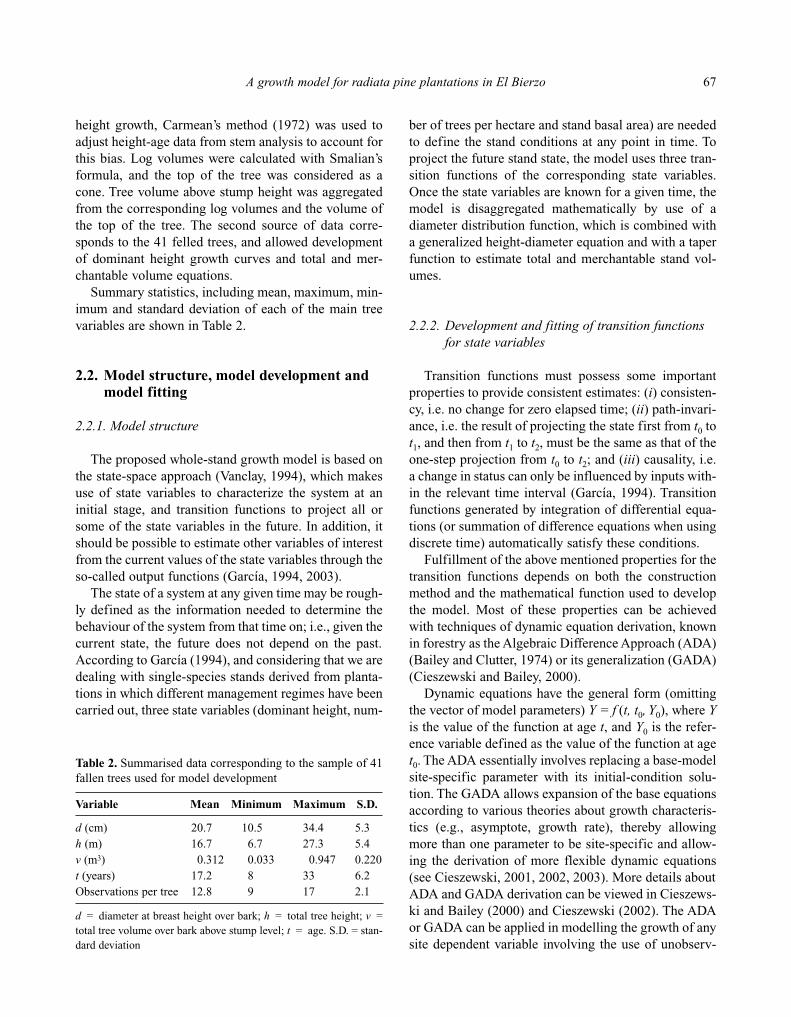
height growth, Carmean’s method (1972) was used toadjust height-age data from stem analysis to account forthis bias. Log volumes were calculated with Smalian’sformula, and the top of the tree was considered as acone. Tree volume above stump height was aggregatedfrom the corresponding log volumes and the volume ofthe top of the tree. The second source of data corre-sponds to the 41 felled trees, and allowed developmentof dominant height growth curves and total and mer-chantable volume equations.Summary statistics, including mean, maximum, min-

imum and standard deviation of each of the main treevariables are shown in Table 2.

2.2. Model structure, model development andmodel fitting

2.2.1. Model structure

The proposed whole-stand growth model is based onthe state-space approach (Vanclay, 1994), which makesuse of state variables to characterize the system at aninitial stage, and transition functions to project all orsome of the state variables in the future. In addition, itshould be possible to estimate other variables of interestfrom the current values of the state variables through theso-called output functions (García, 1994, 2003).The state of a system at any given time may be rough-

ly defined as the information needed to determine thebehaviour of the system from that time on; i.e., given thecurrent state, the future does not depend on the past.According to García (1994), and considering that we aredealing with single-species stands derived from planta-tions in which different management regimes have beencarried out, three state variables (dominant height, num-

Variable Mean Minimum Maximum S.D.

d (cm) 20.7 10.5 34.4 5.3h (m) 16.7 6.7 27.3 5.4v (m3) 0.312 0.033 0.947 0.220t (years) 17.2 8 33 6.2Observations per tree 12.8 9 17 2.1

d = diameter at breast height over bark; h = total tree height; v =total tree volume over bark above stump level; t = age. S.D. = stan-dard deviation

Table 2. Summarised data corresponding to the sample of 41fallen trees used for model development


able variables substituted by the self-referencing con-cept (Northway, 1985) of model definition (Cieszewski,2004), such as stand height, number of trees per unitarea, stand basal area, stand volume, stand biomass orstand carbon sequestration.In the present study, dynamic equations with one and

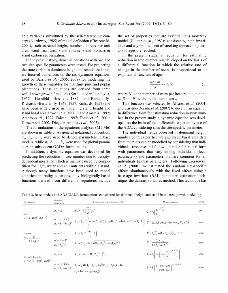
two site-specific parameters were tested. For projectingthe state variables dominant height and stand basal area,we focused our efforts on the six dynamics equationsused by Barrio et al. (2006, 2008) for modelling thegrowth of these variables for maritime pine and poplarplantations. These equations are derived from threewell-known growth functions (Korf –cited in Lundqvist,1957–, Hossfeld –Hossfeld, 1882– and Bertalanffy-Richards –Bertalanffy, 1949, 1957; Richards, 1959) andhave been widely used in modelling stand height andstand basal area growth (e.g. McDill andAmateis, 1992;Amaro et al., 1997; Falcao, 1997; Tomé et al., 2001;Cieszewski, 2002; Diéguez-Aranda et al., 2005).The formulations of the equations analysed (M1-M6)

are shown in Table 3. As general notational convention,a1, a2,…, an were used to denote parameters in basemodels, while b1, b2,…, bm were used for global param-eters in subsequent GADA formulations.In addition, a dynamic equation was developed for

predicting the reduction in tree number due to density-dependent mortality, which is mainly caused by compe-tition for light, water and soil nutrients within a stand.Although many functions have been used to modelempirical mortality equations, only biologically-basedfunctions derived from differential equations include

the set of properties that are essential in a mortalitymodel (Clutter et al., 1983): consistency, path invari-ance and asymptotic limit of stocking approaching zeroas old ages are reached.In the present study, an equation for estimating

reduction in tree number was developed on the basis ofa differential function in which the relative rate ofchange in the number of stems is proportional to anexponential function of age:

(1)

where N is the number of trees per hectare at age t andα, β and δ are the model parameters.This function was selected by Álvarez et al. (2004)

and Castedo-Dorado et al. (2007) to develop an equationin difference form for estimating reduction in stem num-ber. In the present study, a dynamic equation was devel-oped on the basis of this differential equation by use ofthe ADA, considering α as the site-specific parameter.The individual trends observed in dominant height,

number of trees per hectare and stand basal area datafrom the plots can be modelled by considering that indi-viduals’ responses all follow a similar functional formwith parameters that vary among individuals (localparameters) and parameters that are common for allindividuals (global parameters). Following Cieszewskiet al. (2000), we estimated the random site-specificeffects simultaneously with the fixed effects using abase-age invariant (BAI) parameter estimation tech-nique: the dummy variables method. This technique has

Table 3. Base models and ADA/GADA formulations considered for dominant height and stand basal area growth modelling

Base equationParameterrelated to site

Solution for X with initial values (t0,Y0) Dynamic equation Model

Xa =23

01

00 ln at

a

YX =

2

1

0

1

01

b

t

t

b

YbY = (M1)

Korf:

( )321 exp ataaY = ( )Xa exp1 =

Xbba 212 +=( ) ( )( )+±+=

2

00102001021

0 ln4ln 3333 YtbtbYtbtX bbbb

( ) ( )( )30210 expexp btXbbXY += (M2)

Xa =2 = 10

100

3

Y

atX a ( )( )( )2

0011 11 bttYbbY = (M3)Hossfeld:

32

1

1 ata

aY

+=

Xba += 11

Xba 22 = ( )( )3002

210102

10 4 btYbbYbYX +±=

302

01

1 btXb

XbY

++

= (M4)

Xa =2 ( )( ) 01

10021ln tbYX b=

20

21

1

01 11

bttb

b

YbY = (M5)

Bertalanffy-Richards:

( )( ) 3

21 exp1 ataaY =)exp(1 Xa =

Xbba /323 +=)4)(ln(ln

2

1030200200 LbLbYLbYX +=

))exp(1ln( 010 tbL =

)/(

01

10

032

)exp(1

)exp(1Xbb

tb

tbYY

+

= (M6)

tNN

dtdN /


been used in several other studies in fitting growth func-tions for these stand variables (e.g., Diéguez-Aranda etal., 2005; Barrio et al., 2006, 2008; Castedo et al.,2007).In the general formulation of the dynamic equations,

the error terms are assumed to be independent and iden-tically distributed with zero mean. Nevertheless,because of the longitudinal nature of the data sets usedfor model fitting, correlation between the residualswithin the same individual (plot or tree) may be expect-ed. This problem may be especially important in thedevelopment of the dominant height dynamic model onthe basis of data from stem analysis, because of thenumber of measurements corresponding to the sametree. Nevertheless, in the construction of the dynamicequations for reduction in tree number and for basalarea growth, which implies the use of data from the firstand second inventory of 32 plots, the maximum numberof possible time correlations among residuals is practi-cally inexistent, and therefore the problem of autocorre-lated errors can be ignored in the fitting process.To overcome the possible autocorrelation, we mod-

elled the error terms using a continuous time autoregres-sive error structure (CAR(x)), which allows the model tobe applied to irregularly spaced, unbalanced data (Gre-goire et al., 1995; Zimmerman and Núñez-Antón, 2001).To evaluate the presence of autocorrelation and the orderof the CAR(x) to be used, graphs representing residualsplotted against lag-residuals from previous observationswithin each tree or plot were examined visually. Thedummy variables method and the CAR(x) error structurewas programmed by use of the SAS/ETSMODEL pro-cedure (SAS Institute Inc., 2004a), which allows fordynamic updating of the residuals.

2.2.3. Disaggregation system

Diameter distribution

Among the parametric density functions that havebeen used to describe the diameter distribution of astand (e.g., Charlier, Normal, Beta, Gamma, JohnsonSB, Weibull), the Weibull function is the most frequent-ly used, because of its flexibility and simplicity (Cao,2004; Merganic and Sterba, 2006; Palahí et al., 2006).Expression of the Weibull density function is:

(2)

where x is the random variable, a the location parameterdefining the origin of the function, b the scale parame-ter and c the shape parameter controlling the skewness.Of the two basic methodologies used to obtain the

Weibull parameters (parameter estimation and parame-ter recovery), we used the parameter recovery approach,because as stated by several authors (e.g., Cao et al.,1982; Borders and Patterson, 1990; Torres-Rojo et al.,2000; Parresol, 2003) it provides better results thanparameter estimation, even in long-term projections. Torecover the Weibull parameters we used the moments-based parameter recovery method (Burk and Newberry,1984) because it directly warrants that the sum of thedisaggregated basal area obtained by the Weibull func-tion equals the stand basal area provided by an explicitgrowth function of this variable, resulting in numericcompatibility (e.g., Frazier, 1981).In the moments method, the parameters of theWeibull

function are recovered from the first three order momentsof the diameter distribution (i.e. the mean, variance andskewness coefficient, respectively). Alternatively, thelocation parameter (a) may be set to zero. The use of thiscondition restricts the parameters of the Weibull functionto two, therefore making it both easier to model and pro-viding similar results to the three-parameter Weibull, atleast for even-aged, single-species stands (Maltamo et al.,1995; Mabvurira et al., 2002). To recover parameters band c the following expressions were used:

(3)

(4)

where d is the arithmetic mean diameter of the observeddistribution, var is its variance and the Γ is the gammafunction.Once the mean and the variance of the diameter dis-

tribution are known, while taking into account that Eq.3 only depends on parameter c, the latter can beobtained by iterative procedures. Subsequently, parame-ter b can be calculated directly from Eq. 4. As the disag-gregation system is developed for inclusion in a whole-stand growth model, only the arithmetic mean diameterrequires to be modelled, and the variance is directlyobtainable from the arithmetic and the quadratic meandiameter (dg) by use of the relationship var = d2

g - d 2.Hence, the arithmetic mean diameter was modelled with

Eq. 5, which ensures that predictions of d are lower than dg:

c

b

axc

eb

ax

b

cxf =

1

)(

+++

=cc

c

d 11

21

11

var 2

2

2

+=

c

db

11


(5)

Where X is a vector of explanatory variables (e.g.dominant height, number of trees per hectare, age) thatdefine the state of the stand at a specific point in timeand must be obtained from any of the functions of thestand growth model and β is a vector of parameters tobe estimated.A diagram of the disaggregation system including all

the components proposed in the present study is report-ed by Diéguez-Aranda et al., (2006a).

Height estimation for diameter classes

Once the diameter distribution is known, the next stepis the estimation of the height of the average tree in eachdiameter class. Since the height-diameter relationshipvaries from stand to stand due to heterogeneous site con-ditions and silviculture state, and is not constant over timeeven within the same stand (Assmann, 1970), we used ageneralized h-d model which takes into account standvariables that introduce the dynamics of each stand intothe model (e.g., Curtis, 1967; Gadow and Hui, 1999).The generalized h-d model used in the present study

was a modification proposed by Castedo-Dorado et al.(2005b, 2006) on the basis of the Schnute (1981) func-tion, by forcing it to pass through point (0, 1.3), to pre-vent negative height estimates for small trees, and topredict the dominant height of the stand (H) when thediameter at breast height of the subject tree (d) equalsthe dominant diameter of the stand (D0).Parameter estimates were obtained by ordinary least

squares, by application of the Gauss-Newton’s iterativemethod of the SAS/STAT® NLIN procedure (SAS Insti-tute Inc., 2004b).

Total and merchantable volume estimation

Once the diameter and height of the average tree ineach diameter class are estimated, the total tree volumecan be calculated directly by use of a volume equation.Since volume prediction to any merchantable limit isusually required, a taper equation can be used. Integra-tion of a taper equation from the ground to any heightprovides an estimate of the merchantable volume to thatheight (Kozak, 2004).Ideally, a volume estimation system should be com-

patible, i.e., the volume computed by integration of the

taper equation from the ground to the top of the treeshould be equal to that calculated by a total volumeequation (Demaerschalk, 1972; Clutter, 1980). The totalvolume equation is preferred when classification of theproducts by merchantable sizes is not required, therebysimplifying the calculations and making the methodmore suitable for practical purposes.A compatible system was fitted with data correspon-

ding to diameter at different heights and total stem vol-ume from 41 destructively sampled trees. To correct theinherent autocorrelation of the hierarchical data used,the error term was expanded by use of an autoregressivecontinuous model. The presence of autocorrelation andthe order of the CAR(x) to be used were examined asexplained in Section 2.2.2.The compatible volume system of Fang et al. (2000)

was used in this study because it was found to be verysuitable for describing the stem profile and predictingstem volume for different species in several stand struc-tures and regions (Diéguez-Aranda et al., 2006b; Corralet al., 2007), including Pinus radiata (Castedo-Doradoet al., 2007). The fittings were carried out by use of theSAS/ETS® MODEL procedure (SAS Institute Inc.,2004a), which allows for dynamic updating of the resid-uals.Aggregation of total (v) or merchantable (vi) tree vol-

ume times number of trees in each diameter class pro-vides total (V) or merchantable stand volume (Vi),respectively.

2.3. Selection of the best equation in each module

Comparison of the estimates of the different modelsfitted in each module was based on numerical andgraphical analyses. Two statistical criteria obtained fromthe residuals were examined: the coefficient of determi-nation for nonlinear regression (pseudo-R2), showingthe proportion of the total variance of the dependentvariable explained by the model (Ryan, 1997), and theroot mean square error (RMSE), which analyses theaccuracy of the estimates.Other important step in evaluating the models was

graphical analysis of the residuals and examination ofthe appearance of the fitted curves overlaid on the tra-jectories of the dependent variables for each plot. Visu-al or graphical inspection is an essential point in select-ing the most appropriate model because curve profilesmay differ drastically, even though fit statistics andresiduals are similar (e.g., Huang et al., 2003).

Xedd g=


2.4. Overall evaluation of the whole-stand model

Although the behaviour of individual sub-modelswithin the model plays an important role in determin-ing the overall outcome, the validity of each individualcomponent does not guarantee the validity of the over-all outcome, which is usually considered more impor-tant in practice. The overall model outcome musttherefore also be evaluated. The only method that canbe regarded as “true” validation involves the use of anew independent data set (Vanclay and Skovsgaard,1997; Kozak and Kozak, 2003; Yang et al., 2004).However, as new independent data for model valida-tion were not available, only an evaluation of the pre-dictive ability of the overall whole-stand model wascarried out. For that purpose, observed state variablesfrom the first inventory of the 32 plots measured twicewere used to estimate total stand volume at the age ofthe second inventory, including all the components ofthe whole-stand model. It must be taken into accountthat total stand volume is the critical output variable ofthe whole model, since its estimation involves all thefunctions included and is important in economicassessments.In order to assess whether the variance of the predic-

tions is within some tolerance limits, the critical errorstatistic (Ecrit.) was used. The critical error is expressedas a percentage of the observed mean and is computedby re-arranging Freese’s χ 2

n statistic (Reynolds, 1984;Robinson and Froese, 2004):

(6)

where n is the total number of observations in the dataset, is the observed value, ŷi the value predicted fromthe fitted model, y is the average of the observed val-ues, τ is a standard normal deviate at the specifiedprobability level (τ = 1.96 for α = 0.05), and isobtained for α = 0.05 and n degrees of freedom. If thespecified allowable error expressed as a percentage ofthe observed mean is within the limit of the criticalerror, the x 2n test indicates that the model does notgive satisfactory predictions; the contrary result indi-cates that the predictions are acceptable.In addition, plots of observed against predicted val-

ues of stand volume were inspected. If a model isgood, the slope of the regression line betweenobserved and predicted values should pass through theorigin at 45º.

3. Results

3.1. Transition function for state variables

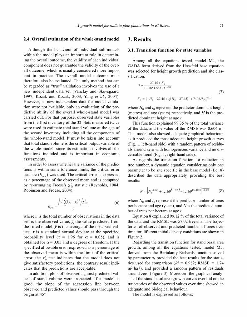
Among all the equations tested, model M4, theGADA form derived from the Hossfeld base equationwas selected for height growth prediction and site clas-sification:

(7)

where H0 and t0 represent the predictor dominant height(metres) and age (years) respectively, and H is the pre-dicted dominant height at age t.This function explained 99.35 % of the total variance

of the data, and the value of the RMSE was 0.604 m.This model also showed adequate graphical behaviour,as it produced the most adequate height growth curves(Fig. 1, left-hand side) with a random pattern of residu-als around zero with homogeneous variance and no dis-cernable trend (Fig. 1, right-hand side).As regards the transition function for reduction in

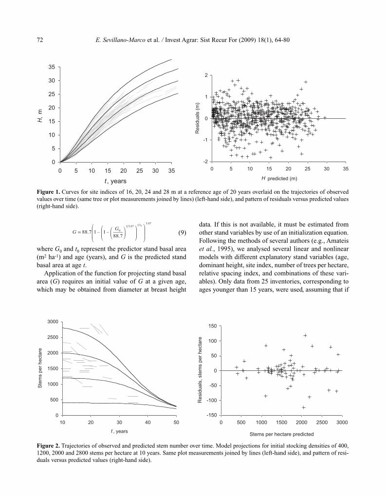
tree number, a dynamic equation considering only oneparameter to be site specific in the base model (Eq. 8)described the data appropriately, providing the bestresults:

(8)

where N0 and t0 represent the predictor number of treesper hectare and age (years), and N is the predicted num-ber of trees per hectare at age t.Equation 8 explained 99.12 % of the total variance of

the data and the RMSE was 57.02 trees/ha. The trajec-tories of observed and predicted number of trees overtime for different initial density conditions are shown inFigure 2.Regarding the transition function for stand basal area

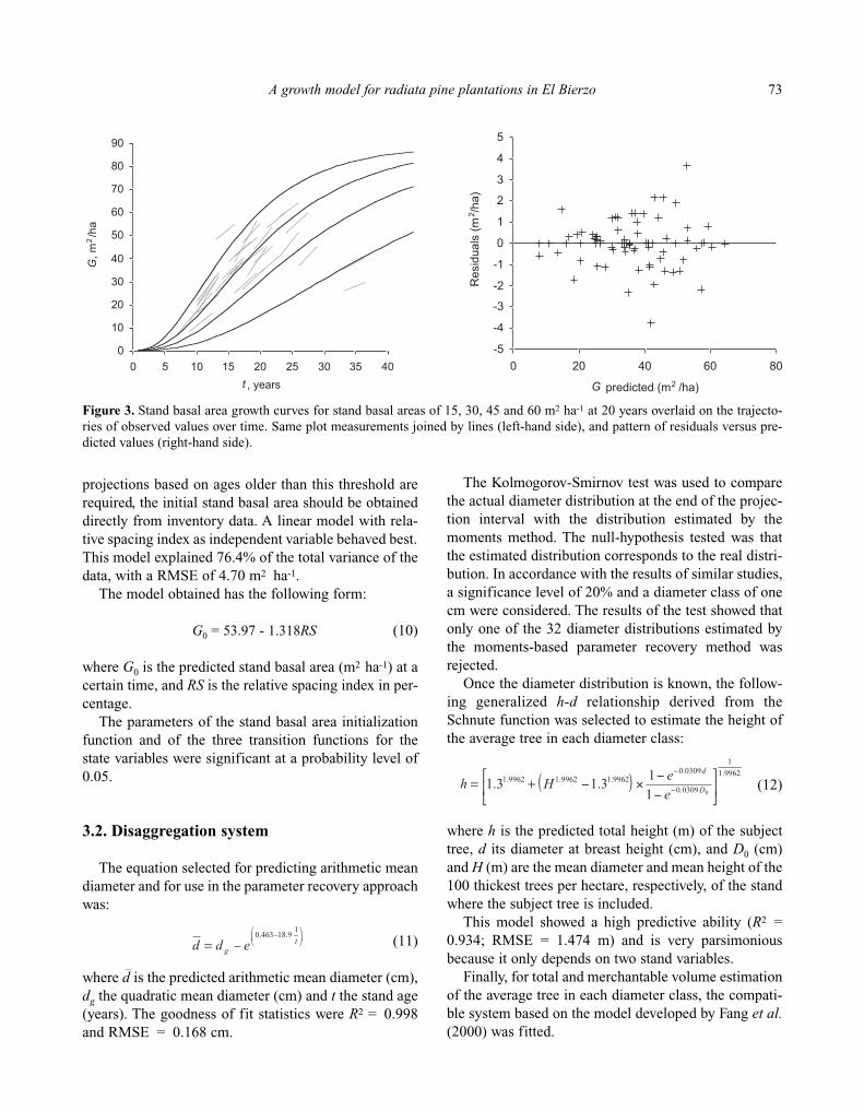
growth, among all the equations tested, model M5,derived from the Bertalanfy-Richards function solvedby parameter a2 provided the best results for the statis-tics used for comparison (R2 = 0.982; RMSE = 1.74m2 ha-1), and provided a random pattern of residualsaround zero (Figure 3). Moreover, the graphical analy-sis of the stand basal area growth curves overlaid on thetrajectories of the observed values over time showed anadequate and biological behaviour.The model is expressed as follows:

( )y

χyyτE

crit

n

iii

crit

2.

1

22

.

ˆ==

522.10

0

5.18511

45.27 +=

tX

XH

( ) ++= 522.100

2002

10 740645.2745.27 tHHHX

( ) ( )[ ] 366.1

1

100100366.10

0169.1169.1+= ttNN


(9)

where G0 and t0 represent the predictor stand basal area(m2 ha-1) and age (years), and G is the predicted standbasal area at age t.Application of the function for projecting stand basal

area (G) requires an initial value of G at a given age,which may be obtained from diameter at breast height

data. If this is not available, it must be estimated fromother stand variables by use of an initialization equation.Following the methods of several authors (e.g., Amateiset al., 1995), we analysed several linear and nonlinearmodels with different explanatory stand variables (age,dominant height, site index, number of trees per hectare,relative spacing index, and combinations of these vari-ables). Only data from 25 inventories, corresponding toages younger than 15 years, were used, assuming that if

07.307.31

0

0

7.88117.88=

tt

GG

0

5

10

15

20

25

30

35

0 5 10 15 20 25 30 35

t , years

H,

m

-2

-1

0

1

2

0 5 10 15 20 25 30 35

H predicted (m)

Res

idua

ls(m

)Figure 1. Curves for site indices of 16, 20, 24 and 28 m at a reference age of 20 years overlaid on the trajectories of observedvalues over time (same tree or plot measurements joined by lines) (left-hand side), and pattern of residuals versus predicted values(right-hand side).

0

500

1000

1500

2000

2500

3000

10 20 30 40 50

t , years

Ste

ms

perh

ecta

re

-150

-100

-50

0

50

100

150

0 500 1000 1500 2000 2500 3000

Stems per hectare predicted

Res

idua

ls,s

tem

spe

rhec

tare

Figure 2. Trajectories of observed and predicted stem number over time. Model projections for initial stocking densities of 400,1200, 2000 and 2800 stems per hectare at 10 years. Same plot measurements joined by lines (left-hand side), and pattern of resi-duals versus predicted values (right-hand side).


projections based on ages older than this threshold arerequired, the initial stand basal area should be obtaineddirectly from inventory data. A linear model with rela-tive spacing index as independent variable behaved best.This model explained 76.4% of the total variance of thedata, with a RMSE of 4.70 m2 ha-1.The model obtained has the following form:

G0 = 53.97 - 1.318RS (10)

where G0 is the predicted stand basal area (m2 ha-1) at acertain time, and RS is the relative spacing index in per-centage.The parameters of the stand basal area initialization

function and of the three transition functions for thestate variables were significant at a probability level of0.05.

3.2. Disaggregation system

The equation selected for predicting arithmetic meandiameter and for use in the parameter recovery approachwas:

(11)

where d is the predicted arithmetic mean diameter (cm),dg the quadratic mean diameter (cm) and t the stand age(years). The goodness of fit statistics were R2 = 0.998and RMSE = 0.168 cm.

The Kolmogorov-Smirnov test was used to comparethe actual diameter distribution at the end of the projec-tion interval with the distribution estimated by themoments method. The null-hypothesis tested was thatthe estimated distribution corresponds to the real distri-bution. In accordance with the results of similar studies,a significance level of 20% and a diameter class of onecm were considered. The results of the test showed thatonly one of the 32 diameter distributions estimated bythe moments-based parameter recovery method wasrejected.Once the diameter distribution is known, the follow-

ing generalized h-d relationship derived from theSchnute function was selected to estimate the height ofthe average tree in each diameter class:

(12)

where h is the predicted total height (m) of the subjecttree, d its diameter at breast height (cm), and D0 (cm)and H (m) are the mean diameter and mean height of the100 thickest trees per hectare, respectively, of the standwhere the subject tree is included.This model showed a high predictive ability (R2 =

0.934; RMSE = 1.474 m) and is very parsimoniousbecause it only depends on two stand variables.Finally, for total and merchantable volume estimation

of the average tree in each diameter class, the compati-ble system based on the model developed by Fang et al.(2000) was fitted.

0

10

20

30

40

50

60

70

80

90

0 5 10 15 20 25 30 35 40t , years

G,m

2/h

a

-5

-4

-3

-2

-1

0

1

2

3

4

5

0 20 40 60 80

G predicted (m2 /ha)

Res

idua

ls(m

2 /ha)

Figure 3. Stand basal area growth curves for stand basal areas of 15, 30, 45 and 60 m2 ha-1 at 20 years overlaid on the trajecto-ries of observed values over time. Same plot measurements joined by lines (left-hand side), and pattern of residuals versus pre-dicted values (right-hand side).

= tg edd

19.18463.0

( ) 9962.1

1

0309.0

0309.09962.19962.19962.1

01

13.13.1 += D

d

e

eHh


This system is constituted by the following compo-nents:Taper function:

(13)

where I1 = 1 if p1 ≤ qi ≤ p2; 0 otherwiseI2 = 1 if p2 < qi ≤ 1; 0 otherwise

p1 and p2 are relative heights from ground level wherethe two inflection points assumed in the model occur

Merchantable volume equation:

(14)

Volume equation:

v = a0da1ha2 (15)

where: d = diameter at breast height over bark (cm); di

= top diameter at height hi over bark (cm); h = total treeheight (m); hi = height above the ground to top diameterdi (m); hst = stump height (m); v = total tree volumeover bark (m3) above stump level; vi = merchantable vol-ume over bark (m3), the volume from stump level to aspecified top diameter di; a0, a1, a2, b1, b2, b3, p1, p2 =regression coefficients to be estimated; k = (π/40 000),metric constant to convert from diameter squared in cmin cm2 to cross-section area in m2; qi = h1 / h.A third-order continuous autoregressive error struc-

ture was necessary to correct the inherent serial autocor-relation of the experimental stem data. The model pro-vided a very good data fit, explaining 98.9% of the totalvariance of di, and the RMSE = 0.847 cm.The resulting parameter estimates were: a0 =

0.000087; a1 = 1.614; a2 = 1.109; b1 = 0.000012; b2 =0.000025; b3 = 0.000035; p1 = 0.05781; p2 = 0.1940.All the parameters of the taper function and of all

other equations corresponding to the disaggregationsystem were significant at a probability level of 0.05.

3.3. Overall evaluation of the whole-stand model

Assessment of model accuracy requirements was car-ried out by comparison between observed volume at the

age of the second inventory and the volume estimatedfrom the whole model. For this purpose, observed dom-inant height, number of trees per hectare and stand basalarea from the first inventory of the 32 plots measuredtwice, served as initial values for the correspondingtransition functions (Eqs. 7, 8 and 9). These functionswere used to project the stand state at the age of the sec-ond inventory. Equation 11 was then used to estimatethe arithmetic mean diameter, which allowed calcula-tion of the variance of the diameter distribution. Equa-tions 3 and 4 were used to recover the Weibull parame-ters, thus allowing estimation of the number of trees ineach diameter class. Finally, equations 12 and 15 wereused to estimate the height and the total volume of theaverage tree in each diameter class respectively. Aggre-gation of total tree volume multiplied by the number oftrees in each diameter class provided total stand volume.A plot of observed against predicted values of stand

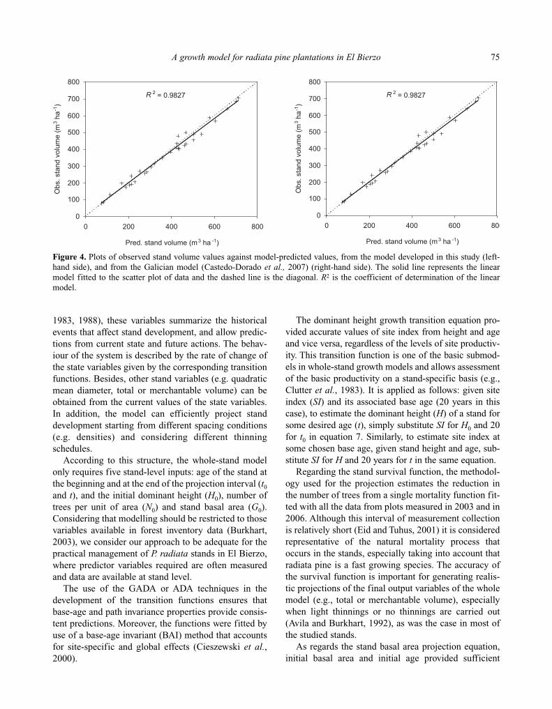
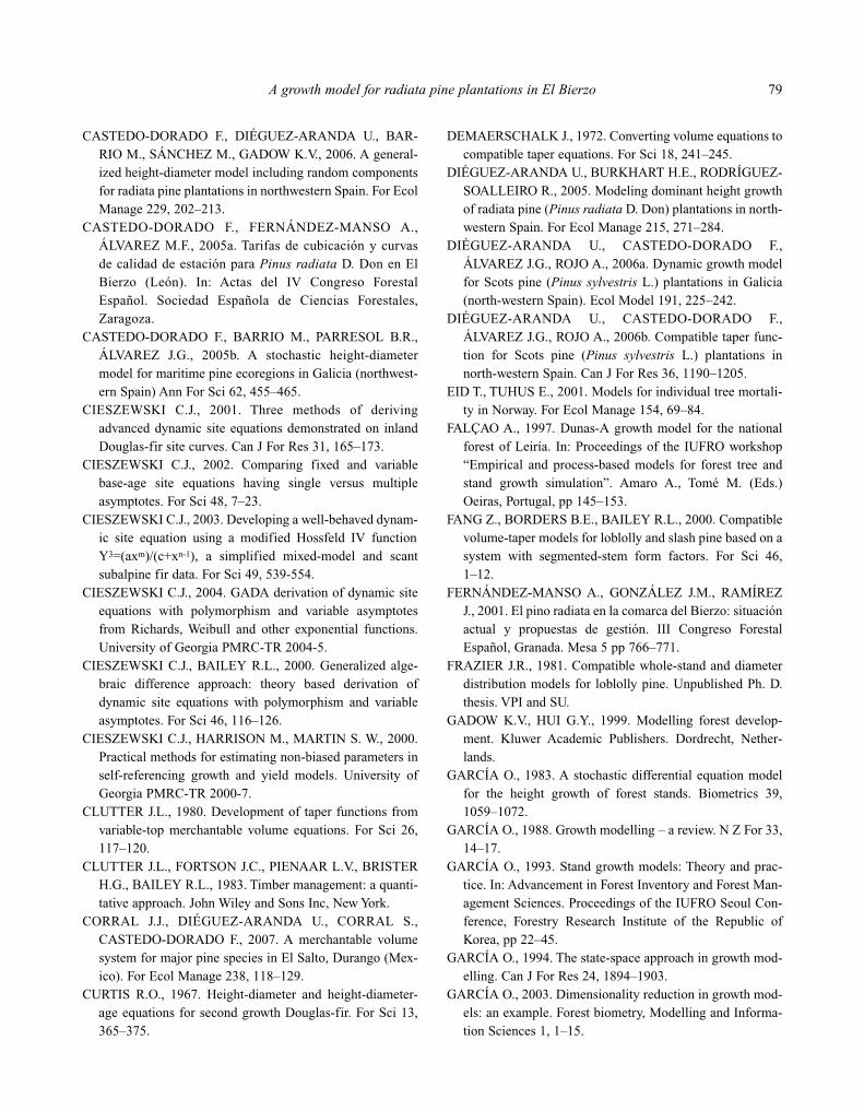
volume obtained following the above procedure for thetime interval considered (3 years) is shown in Figure 4(left-hand side). The linear model fitted for the plotbehaved well (R2 = 0.983), however the plot showedthat there was a slight tendency towards overestimationof stand volume for the prediction interval. A criticalerror of 10.79% was obtained in the projection of totalstand volume for this time interval.The plot of the observed stand volume values against

the values predicted by the model developed with datafrom Galician stands (Castedo-Dorado et al., 2007) isshown in Figure 4 (right-hand side). Although the per-centage variability explained by the linear model fittedfor the scatter plot is high (R2 = 0.978), the Galicianmodel clearly underestimates the stand volume. More-over, the critical error obtained in the projection of standvolume (23.84%) is much higher than that obtained byuse of the local model.

4. Discussion

In this study, a dynamic whole-stand growth modelfor radiata pine plantations in an inland region of Spain(El Bierzo) is presented. The growth model described iscomprehensive because it addresses all forest variablescommonly incorporated in quantitative descriptions offorest growth. The method of construction adopted isrobust because it is based on only three stand variables:dominant height (H), number of trees per hectare (N)and stand basal area (G). In accordance with García’sstate space approach to modelling plantations (García,

( ) ( )( ) 22111211 1 IIIk

ibbk

i qhcd +=

( ) ( ) ( ) ( )( )221121212321122101

21 1 IIIk

ibk

i qrbbIrbbIIrbhcv ++++=

( ) ( )( )

( )( )

( ) 132

23

21

122121 111 0221132

11

bkstbb

kbb

bb

kbbIIII hhrppbbb ==== +

( ) ( ) ( ) ( ) 2132112101

012211

12121 11

rbrrbrrb

hdacprpr

bkaabkbk

++===


1983, 1988), these variables summarize the historicalevents that affect stand development, and allow predic-tions from current state and future actions. The behav-iour of the system is described by the rate of change ofthe state variables given by the corresponding transitionfunctions. Besides, other stand variables (e.g. quadraticmean diameter, total or merchantable volume) can beobtained from the current values of the state variables.In addition, the model can efficiently project standdevelopment starting from different spacing conditions(e.g. densities) and considering different thinningschedules.According to this structure, the whole-stand model

only requires five stand-level inputs: age of the stand atthe beginning and at the end of the projection interval (t0and t), and the initial dominant height (H0), number oftrees per unit of area (N0) and stand basal area (G0).Considering that modelling should be restricted to thosevariables available in forest inventory data (Burkhart,2003), we consider our approach to be adequate for thepractical management of P. radiata stands in El Bierzo,where predictor variables required are often measuredand data are available at stand level.The use of the GADA or ADA techniques in the

development of the transition functions ensures thatbase-age and path invariance properties provide consis-tent predictions. Moreover, the functions were fitted byuse of a base-age invariant (BAI) method that accountsfor site-specific and global effects (Cieszewski et al.,2000).

The dominant height growth transition equation pro-vided accurate values of site index from height and ageand vice versa, regardless of the levels of site productiv-ity. This transition function is one of the basic submod-els in whole-stand growth models and allows assessmentof the basic productivity on a stand-specific basis (e.g.,Clutter et al., 1983). It is applied as follows: given siteindex (SI) and its associated base age (20 years in thiscase), to estimate the dominant height (H) of a stand forsome desired age (t), simply substitute SI for H0 and 20for t0 in equation 7. Similarly, to estimate site index atsome chosen base age, given stand height and age, sub-stitute SI for H and 20 years for t in the same equation.Regarding the stand survival function, the methodol-

ogy used for the projection estimates the reduction inthe number of trees from a single mortality function fit-ted with all the data from plots measured in 2003 and in2006. Although this interval of measurement collectionis relatively short (Eid and Tuhus, 2001) it is consideredrepresentative of the natural mortality process thatoccurs in the stands, especially taking into account thatradiata pine is a fast growing species. The accuracy ofthe survival function is important for generating realis-tic projections of the final output variables of the wholemodel (e.g., total or merchantable volume), especiallywhen light thinnings or no thinnings are carried out(Avila and Burkhart, 1992), as was the case in most ofthe studied stands.As regards the stand basal area projection equation,

initial basal area and initial age provided sufficient

R 2 = 0.9827

0

100

200

300

400

500

600

700

800

0 200 400 600 800

Pred. stand volume (m3 ha -1)

Obs

.sta

ndvo

lum

e(m

3ha

-1)

R 2 = 0.9827

0

100

200

300

400

500

600

700

800

0 200 400 600 800

Pred. stand volume (m3 ha -1)

Obs

.sta

ndvo

lum

e(m

3ha

-1)

Figure 4. Plots of observed stand volume values against model-predicted values, from the model developed in this study (left-hand side), and from the Galician model (Castedo-Dorado et al., 2007) (right-hand side). The solid line represents the linearmodel fitted to the scatter plot of data and the dashed line is the diagonal. R2 is the coefficient of determination of the linearmodel.


information about the future trajectory of the basal areaof the stand, regardless of initial spacing, thinning histo-ry or site quality. This can be explained because standbasal area and age are good enough estimators of qual-ity in stands where silviculture is applied next to forestdynamics with low thinning (Bravo-Oviedo et al.,2004). The basal area initialization function developedshould only be used to predict this variable in standssimilar to those where the experimental data were col-lected, i.e., unthinned or lightly thinned stands youngerthan 15 years. The initialization and the projection func-tion are not compatible because of the variation overtime in the relative spacing index. This incompatibilityis not a major problem, as the initialization functionwould only be used when no inventory data are available(Amateis et al., 1995).Explanatory variables of the components of the dis-

aggregation system can be easily obtained at any pointin time from the three transition functions previouslymentioned. The only exception is dominant diameter ofthe generalized h-d relationship, which is a difficultvariable to project (Lappi, 1997), and must be estimatedfrom the diameter distribution.Total stand volume was selected in the present study

as the critical output variable for the whole-standgrowth model, although other stand variables can beassessed on the basis of this model. For instance, with-in the framework of climate change challenges, anincreasing interest in studying the amount of biomassand carbon sequestration through forest management isexpected and could be adequately tackled using themodel. For example, if biomass equations that includethe diameter at breast height and the total height as inde-pendent variables are developed for this species theycan be easily incorporated into the disaggregation sys-tem proposed and converted in carbon pools (e.g., Meri-no et al., 2005).

Considering the required accuracy in forest growthmodelling at stand-level, where a mean prediction errorof the observed mean at 95% confidence intervals with-in ± 10%-20% is generally realistic and reasonable as alimit for the actual choice of acceptance and rejectionlevels (Huang et al., 2003), it can be stated that, on thebasis of the critical error statistic obtained (10.79%), themodel developed in this study provides satisfactory pre-dictions.Taking the same criterion into account, the model

developed from the Galician data (Castedo-Dorado etal., 2007) cannot be applied directly to the region of ElBierzo, since the critical error statistics obtained in this

case (23.84%) is higher than the upper limit usuallyconsidered for acceptance of a model. This result isexpected a priori, since a fitted model is likely to pro-duce errors when used on a local data set different fromthe data used in its construction (Huang, 2002). More-over, these results also justify the need to adapt the Gali-cian model, refitting the individual submodels on thebasis of local (El Bierzo) data.In summary, the overall evaluation of the model

developed for El Bierzo demonstrates that it is robust, atleast for short term projections of stand volume. Thischaracteristic is especially interesting for planning pur-poses in fast growing species, as is the case here. As thestudy is based on stands of ages between 7-36 years,predictions for stands less than 7-years or more than 36years-old should be used with caution.

5.Applications and conclusions

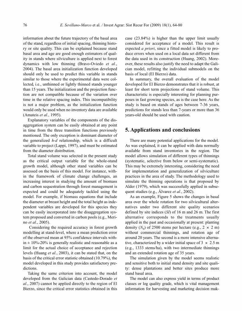
There are many potential applications for the model.As was explained, it can be applied with data normallyavailable from stand inventories in the region. Themodel allows simulation of different types of thinnings(systematic, selective from below or semi-systematic).This may be extremely interesting, considering the needfor implementation and generalization of silviculturepractices in the area of study. The methodology used tosimulate the thinning operations is that proposed byAlder (1979), which was successfully applied in subse-quent studies (e.g., Álvarez et al., 2002).As an example, Figure 5 shows the changes in basal

area over the whole rotation for two silvicultural alter-natives under two different site quality scenariosdefined by site indices (SI) of 16 m and 26 m. The firstalternative corresponds to the treatments usuallyapplied in the past and occasionally at present: plantingdensity (N0) of 2500 stems per hectare (e.g., 2 × 2 m)without commercial thinnings, and rotation age ofaround 20 years. The second is a more intensive alterna-tive, characterized by a wider initial space of 3 × 2.5 m(e.g., 1333 stems/ha), with two intermediate thinningsand an extended rotation age of 35 years.The simulation given by the model seems realistic

and sensitive both to initial stand density and site quali-ty: dense plantations and better sites produce morestand basal area.The model can also express yield in terms of product

classes or log quality grade, which is vital managementinformation for harvesting and marketing decision mak-


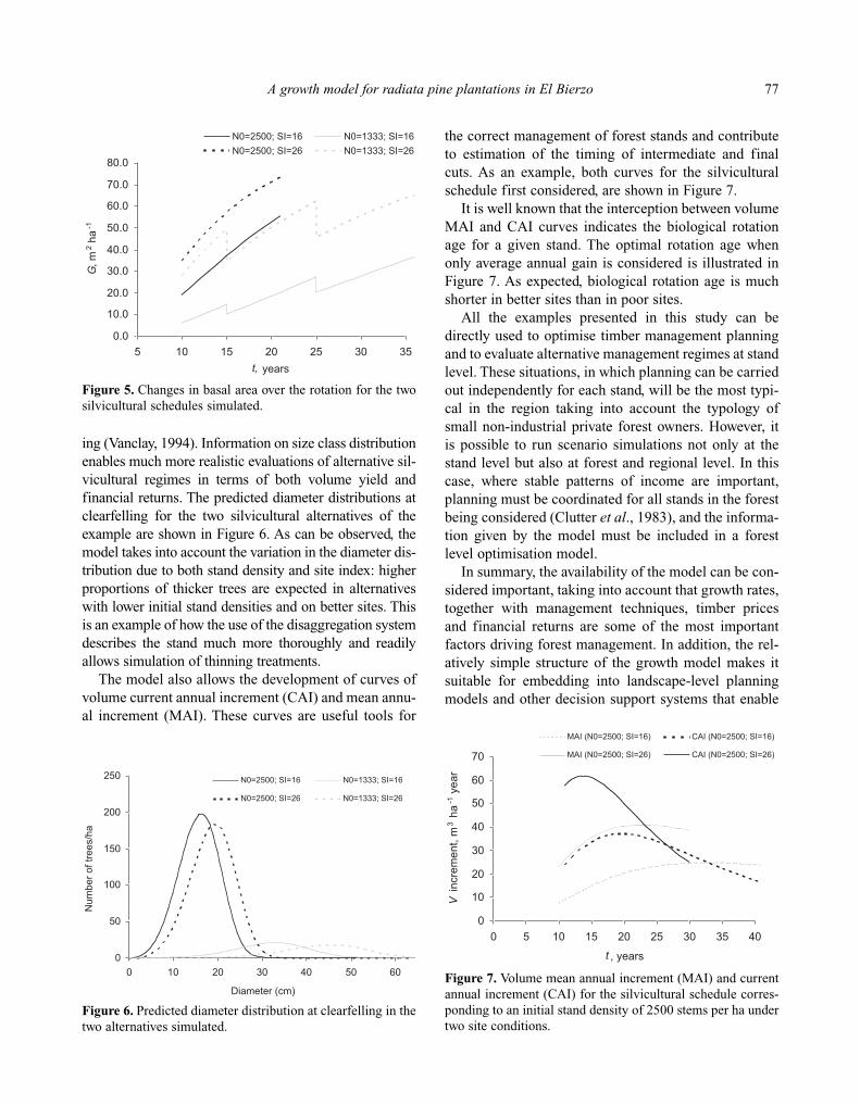
ing (Vanclay, 1994). Information on size class distributionenables much more realistic evaluations of alternative sil-vicultural regimes in terms of both volume yield andfinancial returns. The predicted diameter distributions atclearfelling for the two silvicultural alternatives of theexample are shown in Figure 6. As can be observed, themodel takes into account the variation in the diameter dis-tribution due to both stand density and site index: higherproportions of thicker trees are expected in alternativeswith lower initial stand densities and on better sites. Thisis an example of how the use of the disaggregation systemdescribes the stand much more thoroughly and readilyallows simulation of thinning treatments.The model also allows the development of curves of

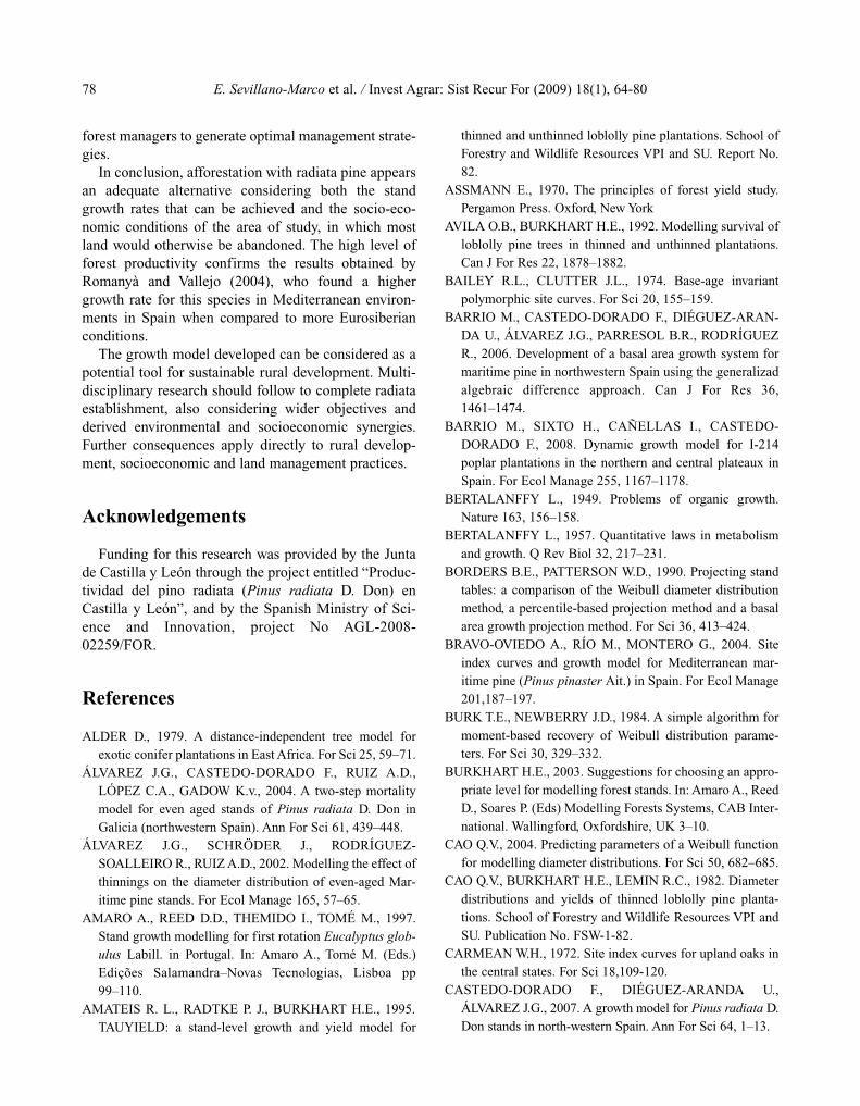
volume current annual increment (CAI) and mean annu-al increment (MAI). These curves are useful tools for

the correct management of forest stands and contributeto estimation of the timing of intermediate and finalcuts. As an example, both curves for the silviculturalschedule first considered, are shown in Figure 7.It is well known that the interception between volume

MAI and CAI curves indicates the biological rotationage for a given stand. The optimal rotation age whenonly average annual gain is considered is illustrated inFigure 7. As expected, biological rotation age is muchshorter in better sites than in poor sites.All the examples presented in this study can be

directly used to optimise timber management planningand to evaluate alternative management regimes at standlevel. These situations, in which planning can be carriedout independently for each stand, will be the most typi-cal in the region taking into account the typology ofsmall non-industrial private forest owners. However, itis possible to run scenario simulations not only at thestand level but also at forest and regional level. In thiscase, where stable patterns of income are important,planning must be coordinated for all stands in the forestbeing considered (Clutter et al., 1983), and the informa-tion given by the model must be included in a forestlevel optimisation model.In summary, the availability of the model can be con-

sidered important, taking into account that growth rates,together with management techniques, timber pricesand financial returns are some of the most importantfactors driving forest management. In addition, the rel-atively simple structure of the growth model makes itsuitable for embedding into landscape-level planningmodels and other decision support systems that enable

0.0

10.0

20.0

30.0

40.0

50.0

60.0

70.0

80.0

5 10 15 20 25 30 35t, years

G,m

2ha

-1

N0=2500; SI=16 N0=1333; SI=16N0=2500; SI=26 N0=1333; SI=26

Figure 5. Changes in basal area over the rotation for the twosilvicultural schedules simulated.

0

50

100

150

200

250

0 10 20 30 40 50 60

Diameter (cm)

Num

bero

ftre

es/h

a

N0=2500; SI=16 N0=1333; SI=16

N0=2500; SI=26 N0=1333; SI=26

Figure 6. Predicted diameter distribution at clearfelling in thetwo alternatives simulated.

0

10

20

30

40

50

60

70

0 5 10 15 20 25 30 35 40

t , years

Vin

crem

ent,

m3

ha-1

year

MAI (N0=2500; SI=16) CAI (N0=2500; SI=16)

MAI (N0=2500; SI=26) CAI (N0=2500; SI=26)

Figure 7. Volume mean annual increment (MAI) and currentannual increment (CAI) for the silvicultural schedule corres-ponding to an initial stand density of 2500 stems per ha undertwo site conditions.


forest managers to generate optimal management strate-gies.In conclusion, afforestation with radiata pine appears

an adequate alternative considering both the standgrowth rates that can be achieved and the socio-eco-nomic conditions of the area of study, in which mostland would otherwise be abandoned. The high level offorest productivity confirms the results obtained byRomanyà and Vallejo (2004), who found a highergrowth rate for this species in Mediterranean environ-ments in Spain when compared to more Eurosiberianconditions.The growth model developed can be considered as a

potential tool for sustainable rural development. Multi-disciplinary research should follow to complete radiataestablishment, also considering wider objectives andderived environmental and socioeconomic synergies.Further consequences apply directly to rural develop-ment, socioeconomic and land management practices.

Acknowledgements

Funding for this research was provided by the Juntade Castilla y León through the project entitled “Produc-tividad del pino radiata (Pinus radiata D. Don) enCastilla y León”, and by the Spanish Ministry of Sci-ence and Innovation, project No AGL-2008-02259/FOR.

References

ALDER D., 1979. A distance-independent tree model forexotic conifer plantations in EastAfrica. For Sci 25, 59–71.

ÁLVAREZ J.G., CASTEDO-DORADO F., RUIZ A.D.,LÓPEZ C.A., GADOW K.v., 2004. A two-step mortalitymodel for even aged stands of Pinus radiata D. Don inGalicia (northwestern Spain). Ann For Sci 61, 439–448.

ÁLVAREZ J.G., SCHRÖDER J., RODRÍGUEZ-SOALLEIRO R., RUIZA.D., 2002. Modelling the effect ofthinnings on the diameter distribution of even-aged Mar-itime pine stands. For Ecol Manage 165, 57–65.

AMARO A., REED D.D., THEMIDO I., TOMÉ M., 1997.Stand growth modelling for first rotation Eucalyptus glob-ulus Labill. in Portugal. In: Amaro A., Tomé M. (Eds.)Edições Salamandra–Novas Tecnologias, Lisboa pp99–110.

AMATEIS R. L., RADTKE P. J., BURKHART H.E., 1995.TAUYIELD: a stand-level growth and yield model for

thinned and unthinned loblolly pine plantations. School ofForestry and Wildlife Resources VPI and SU. Report No.82.

ASSMANN E., 1970. The principles of forest yield study.Pergamon Press. Oxford, NewYork

AVILA O.B., BURKHART H.E., 1992. Modelling survival ofloblolly pine trees in thinned and unthinned plantations.Can J For Res 22, 1878–1882.

BAILEY R.L., CLUTTER J.L., 1974. Base-age invariantpolymorphic site curves. For Sci 20, 155–159.

BARRIO M., CASTEDO-DORADO F., DIÉGUEZ-ARAN-DA U., ÁLVAREZ J.G., PARRESOL B.R., RODRÍGUEZR., 2006. Development of a basal area growth system formaritime pine in northwestern Spain using the generalizadalgebraic difference approach. Can J For Res 36,1461–1474.

BARRIO M., SIXTO H., CAÑELLAS I., CASTEDO-DORADO F., 2008. Dynamic growth model for I-214poplar plantations in the northern and central plateaux inSpain. For Ecol Manage 255, 1167–1178.

BERTALANFFY L., 1949. Problems of organic growth.Nature 163, 156–158.

BERTALANFFY L., 1957. Quantitative laws in metabolismand growth. Q Rev Biol 32, 217–231.

BORDERS B.E., PATTERSON W.D., 1990. Projecting standtables: a comparison of the Weibull diameter distributionmethod, a percentile-based projection method and a basalarea growth projection method. For Sci 36, 413–424.

BRAVO-OVIEDO A., RÍO M., MONTERO G., 2004. Siteindex curves and growth model for Mediterranean mar-itime pine (Pinus pinaster Ait.) in Spain. For Ecol Manage201,187–197.

BURK T.E., NEWBERRY J.D., 1984. A simple algorithm formoment-based recovery of Weibull distribution parame-ters. For Sci 30, 329–332.

BURKHART H.E., 2003. Suggestions for choosing an appro-priate level for modelling forest stands. In: AmaroA., ReedD., Soares P. (Eds) Modelling Forests Systems, CAB Inter-national. Wallingford, Oxfordshire, UK 3–10.

CAO Q.V., 2004. Predicting parameters of a Weibull functionfor modelling diameter distributions. For Sci 50, 682–685.

CAO Q.V., BURKHART H.E., LEMIN R.C., 1982. Diameterdistributions and yields of thinned loblolly pine planta-tions. School of Forestry and Wildlife Resources VPI andSU. Publication No. FSW-1-82.

CARMEANW.H., 1972. Site index curves for upland oaks inthe central states. For Sci 18,109-120.

CASTEDO-DORADO F., DIÉGUEZ-ARANDA U.,ÁLVAREZ J.G., 2007. A growth model for Pinus radiata D.Don stands in north-western Spain. Ann For Sci 64, 1–13.


CASTEDO-DORADO F., DIÉGUEZ-ARANDA U., BAR-RIO M., SÁNCHEZ M., GADOW K.V., 2006. A general-ized height-diameter model including random componentsfor radiata pine plantations in northwestern Spain. For EcolManage 229, 202–213.

CASTEDO-DORADO F., FERNÁNDEZ-MANSO A.,ÁLVAREZ M.F., 2005a. Tarifas de cubicación y curvasde calidad de estación para Pinus radiata D. Don en ElBierzo (León). In: Actas del IV Congreso ForestalEspañol. Sociedad Española de Ciencias Forestales,Zaragoza.

CASTEDO-DORADO F., BARRIO M., PARRESOL B.R.,ÁLVAREZ J.G., 2005b. A stochastic height-diametermodel for maritime pine ecoregions in Galicia (northwest-ern Spain) Ann For Sci 62, 455–465.

CIESZEWSKI C.J., 2001. Three methods of derivingadvanced dynamic site equations demonstrated on inlandDouglas-fir site curves. Can J For Res 31, 165–173.

CIESZEWSKI C.J., 2002. Comparing fixed and variablebase-age site equations having single versus multipleasymptotes. For Sci 48, 7–23.

CIESZEWSKI C.J., 2003. Developing a well-behaved dynam-ic site equation using a modified Hossfeld IV functionY3=(axm)/(c+xn-1), a simplified mixed-model and scantsubalpine fir data. For Sci 49, 539-554.

CIESZEWSKI C.J., 2004. GADA derivation of dynamic siteequations with polymorphism and variable asymptotesfrom Richards, Weibull and other exponential functions.University of Georgia PMRC-TR 2004-5.

CIESZEWSKI C.J., BAILEY R.L., 2000. Generalized alge-braic difference approach: theory based derivation ofdynamic site equations with polymorphism and variableasymptotes. For Sci 46, 116–126.

CIESZEWSKI C.J., HARRISON M., MARTIN S. W., 2000.Practical methods for estimating non-biased parameters inself-referencing growth and yield models. University ofGeorgia PMRC-TR 2000-7.

CLUTTER J.L., 1980. Development of taper functions fromvariable-top merchantable volume equations. For Sci 26,117–120.

CLUTTER J.L., FORTSON J.C., PIENAAR L.V., BRISTERH.G., BAILEY R.L., 1983. Timber management: a quanti-tative approach. John Wiley and Sons Inc, NewYork.

CORRAL J.J., DIÉGUEZ-ARANDA U., CORRAL S.,CASTEDO-DORADO F., 2007. A merchantable volumesystem for major pine species in El Salto, Durango (Mex-ico). For Ecol Manage 238, 118–129.

CURTIS R.O., 1967. Height-diameter and height-diameter-age equations for second growth Douglas-fir. For Sci 13,365–375.

DEMAERSCHALK J., 1972. Converting volume equations tocompatible taper equations. For Sci 18, 241–245.

DIÉGUEZ-ARANDA U., BURKHART H.E., RODRÍGUEZ-SOALLEIRO R., 2005. Modeling dominant height growthof radiata pine (Pinus radiata D. Don) plantations in north-western Spain. For Ecol Manage 215, 271–284.

DIÉGUEZ-ARANDA U., CASTEDO-DORADO F.,ÁLVAREZ J.G., ROJO A., 2006a. Dynamic growth modelfor Scots pine (Pinus sylvestris L.) plantations in Galicia(north-western Spain). Ecol Model 191, 225–242.

DIÉGUEZ-ARANDA U., CASTEDO-DORADO F.,ÁLVAREZ J.G., ROJO A., 2006b. Compatible taper func-tion for Scots pine (Pinus sylvestris L.) plantations innorth-western Spain. Can J For Res 36, 1190–1205.

EID T., TUHUS E., 2001. Models for individual tree mortali-ty in Norway. For Ecol Manage 154, 69–84.

FALÇAO A., 1997. Dunas-A growth model for the nationalforest of Leiría. In: Proceedings of the IUFRO workshop“Empirical and process-based models for forest tree andstand growth simulation”. Amaro A., Tomé M. (Eds.)Oeiras, Portugal, pp 145–153.

FANG Z., BORDERS B.E., BAILEY R.L., 2000. Compatiblevolume-taper models for loblolly and slash pine based on asystem with segmented-stem form factors. For Sci 46,1–12.

FERNÁNDEZ-MANSO A., GONZÁLEZ J.M., RAMÍREZJ., 2001. El pino radiata en la comarca del Bierzo: situaciónactual y propuestas de gestión. III Congreso ForestalEspañol, Granada. Mesa 5 pp 766–771.

FRAZIER J.R., 1981. Compatible whole-stand and diameterdistribution models for loblolly pine. Unpublished Ph. D.thesis. VPI and SU.

GADOW K.V., HUI G.Y., 1999. Modelling forest develop-ment. Kluwer Academic Publishers. Dordrecht, Nether-lands.

GARCÍA O., 1983. A stochastic differential equation modelfor the height growth of forest stands. Biometrics 39,1059–1072.

GARCÍA O., 1988. Growth modelling – a review. N Z For 33,14–17.

GARCÍA O., 1993. Stand growth models: Theory and prac-tice. In: Advancement in Forest Inventory and Forest Man-agement Sciences. Proceedings of the IUFRO Seoul Con-ference, Forestry Research Institute of the Republic ofKorea, pp 22–45.

GARCÍA O., 1994. The state-space approach in growth mod-elling. Can J For Res 24, 1894–1903.

GARCÍA O., 2003. Dimensionality reduction in growth mod-els: an example. Forest biometry, Modelling and Informa-tion Sciences 1, 1–15.


GREGOIRE T.G., SCHABENBERGER O., BARRETT J.P.,1995. Linear modelling of irregularly spaced, unbalanced,longitudinal data from permanent-plot measurements. CanJ For Res 25, 137–156.

HOSSFELD J.W., 1882. Mathematik für Forstmänner,Ökonomen und Cameralisten. Gotha, 4 Bd, pp 310.

HUANG S., 2002. Validating and localizing growth and yieldmodels: procedures, problems and prospects. In: AmaroA., Reed D., Soares P., (Eds.). Workshop on reality, modelsand parameter estimation – the forestry scenario. Sesimbra(Portugal).

HUANG S.,YANGY., WANGY., 2003. A critical look at pro-cedures for validating growth and yield models. In: AmaroA, Reed D, Soares P (Eds.) Modelling forest systems. CABInternational, Wallingford, Oxfordshire, UK, pp 271–293.

KOTZE H., 2003. A strategy for growth and yield research inpine and eucalipt plantations in Komatiland Forests inSouth Africa. In: Amaro A., Reed D., Soares P. (Eds) Mod-elling Forest Systems, CAB International, Wallingford,Oxfordshire, UK, pp 75–84.

KOZAK A., 2004. My last words on taper functions. ForChron 80, 507–515.

KOZAKA., KOZAK R., 2003. Does cross validation provideadditional information in the evaluation of regression mod-els? Can J For Res 33, 976–987.

LAPPI J., 1997. A longitudinal analysis of height/diametercurves. For Sci 43, 555–570.

LUNDQVIST B., 1957. On the height growth in cultivatedstands of pine and spruce in northern Sweden. Medd FranStatens Skogforsk 47, 1–64.

MABVURIRA D., MALTAMO M., KANGASA., 2002. Pre-dicting and calibrating diameter distributions of Eucalyp-tus grandis (Hill) Maiden plantations in Zimbabwe. NewFor 23, 207–223.

MALTAMO M., PUUMALAINEN J., PÄIVINEN R., 1995.Comparison of Beta and Weibull functions for modellingbasal area diameter distributions in stands of Pinussylvestris and Picea abies. Scand J For Res 10, 284–295.

MCDILL M.E., AMATEIS R.I., 1992. Measuring forest sitequality using the parameters of a dimensionally compatibleheight growth function. For Sci 38, 409–429.

MERGANIC J., STERBA H., 2006. Characterisation of diam-eter distribution using the Weibull function: method ofmoments. Eur J For Res 125, 427–439.

MERINO A., BALBOA M.A., RODRÍGUEZ R., ÁLVAREZJ.G., 2005. Nutrient exports under different harvestingregimes in fast-growing forest plantations in southernEurope. For Ecol Manage 207, 325–339.

NORTHWAY S.M., 1985. Fitting site index equations andother selfreferencing functions. For Sci 31, 233–235.

PALAHÍ M., PUKKALA T., TRASOBARES T., 2006. Mod-elling the diameter distribution of Pinus sylvestris, Pinusnigra and Pinus halepensis forest stands in Catalonia usingthe truncated Weibull function. Forestry 79, 553–562.

PARRESOL B.R., 2003. Recovering parameters of Johnson’sSB distribution. USDA Forest Service. Res Pap SRS-31.

REYNOLDS M.R., 1984. Estimating the error in model pre-dictions. For Sci 30, 454–469.

RICHARDS F.J., 1959. A flexible growth function for empir-ical use. J Exp Bot 10, 290–300.

ROBINSON A.P., FROESE R.E., 2004. Model validationusing equivalence tests. Ecol Model 176, 349–358.

ROMANYÀ J., VALLEJO V.R., 2004. Productivity of Pinusradiata plantations in Spain in response to climate and soil.For Ecol Manage 195, 177–189.

RYAN T.P., 1997. Modern regression methods. John Wileyand Sons Inc, NewYork.

SAS Institute Inc., 2004a. SAS/ETS® 9.1 User’s guide. Cary,NC: SAS Institute Inc. USA.

SAS Institute Inc., 2004b. SAS/STAT® 9.1 User’s guide. Cary,NC: SAS Institute Inc. USA.

SCHNUTE J., 1981.A versatile growth model with statistical-ly stable parameters. Can J Fish Aquatic Sci 38,1128–1140.

SUTTON W.R.J., 1999. The need for planted forests and theexample of radiata pine. New For 17, 95–109.

TOMÉ M., RIBEIRO F., SOARES P., 2001. O modelo Glob-ulus 2.1. Relatorios Técnicocientíficos do GIMREF,nº1/2001. Universidade Técnica de Lisboa, Instituto Supe-rior deAgronomía, Departamento de Engenharia Florestal,69 pp.

TORRES-ROJO J.M., MAGAÑA-TORRES O.S., ACOSTA-MIRELES M., 2000. Metodología para mejorar la predic-ción de parámetros de distribuciones diamétricas. Agro-ciencia 34, 627–637.

TRINCADO G.V., QUEZADA P.R., GADOW K.V., 2003. Acomparison of two stand table projection methods foryoung Eucalyptus nitens (Maiden) plantations in Chile. ForEcol Manage 180, 443–451.

VANCLAY J.K., 1994. Modelling forest growth and yield.Applications to mixed tropical forests. CAB International.Wallingford, UK.

VANCLAY J.K., SKOVSGAARD J.P., 1997. Evaluation for-est growth models. Ecol Model 98, 1–12.

YANGY., MONSERUD R.A., HUANG S., 2004. An evalua-tion of diagnostic test and their roles in validating forestbiometric models. Can J For Res 34, 619–629.

ZIMMERMAN D.L., NÚÑEZ-ANTÓN V., 2001. Parametricmodelling of growth curve data: an overview (with discus-sion). Test 10, 1–73.

Documents

Developmentandapplicationsofagrowthmodelfor Pinus radiata ... · AgrowthmodelforradiatapineplantationsinElBierzo 67 beroftreesperhectareandstandbasalarea)areneeded todefinethestandconditionsatanypointintime.To