Development of Vision-aided Navigation for aWearable Outdoor Augmented Reality System

Alberico Menozzi∗, Brian Clipp†, Eric Wenger∗, Jared Heinly‡,Enrique Dunn‡, Herman Towles∗, Jan-Michael Frahm‡, Gregory Welch§

∗Applied Research Associates, Inc. (ARA), Raleigh, NC 27615 – Email: amenozzi@ara.com†URC Ventures, Redmond, WA – Email: bclipp@gmail.com

‡University of North Carolina, Chapel Hill, NC – Email: jmf@cs.unc.edu§University of Central Florida, Orlando, FL – Email: welch@ucf.edu

Abstract—This paper describes the development of vision-aided navigation (i.e., pose estimation) for a wearable augmentedreality system operating in natural outdoor environments. Thissystem combines a novel pose estimation capability, a helmet-mounted see-through display, and a wearable processing unit toaccurately overlay geo-registered graphics on the user’s view ofreality. Accurate pose estimation is achieved through integrationof inertial, magnetic, GPS, terrain elevation data, and computer-vision inputs. Specifically, a helmet-mounted forward-lookingcamera and custom computer vision algorithms are used toprovide measurements of absolute orientation (i.e., orientationof the helmet with respect to the Earth). These orientation mea-surements, which leverage mountainous terrain horizon geometryand/or known landmarks, enable the system to achieve significantimprovements in accuracy compared to GPS/INS solutions ofsimilar size, weight, and power, and to operate robustly in thepresence of magnetic disturbances. Recent field testing activities,across a variety of environments where these vision-based signalsof opportunity are available, indicate that high accuracy (lessthan 10 mrad) in graphics geo-registration can be achieved. Thispaper presents the pose estimation process, the methods behindthe generation of vision-based measurements, and representativeexperimental results.

Index Terms—inertial navigation, augmented reality, computervision.

I. INTRODUCTION

In his 2009 review [1], Welch stated that the “Holy Grail”for researchers working on tracking for augmented reality(AR) “still seems to be robust and accurate tracking outdoors,for augmented reality everywhere. Researchers around theworld are working on 6 DOF position and orientation-awarecomputer interfaces that will support access to informationembedded in or attached to the physical world all around us.”At around the same time, the effort described in this paperstarted, with the specific objective of developing a wearableAR system to provide intuitive visualization of geo-registeredgraphics on a see-through display. The core challenge hasindeed been to achieve robust and accurate estimation of pose(i.e., position and orientation) outdoors.

In this particular application, the pose estimation problemis challenging on numerous fronts. The system must (a) trackthe pose of the user’s head quickly and precisely (latency isvery obvious when looking through a see-through display), (b)do so using relatively low-cost, low-SWAP (size, weight, andpower) hardware in a ruggedized package, and (c) operate

(a) (b)

(c) (d)

3

1

1

3

2

2

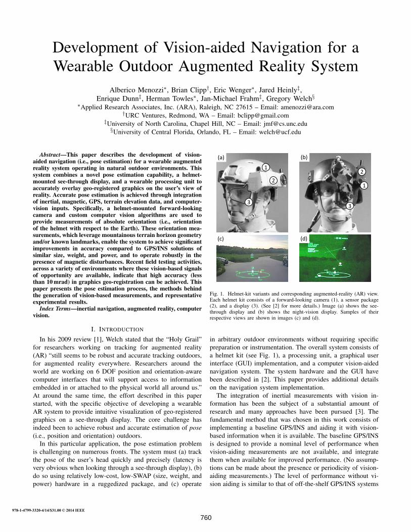
Fig. 1. Helmet-kit variants and corresponding augmented-reality (AR) view.Each helmet kit consists of a forward-looking camera (1), a sensor package(2), and a display (3). (See [2] for more details.) Image (a) shows the see-through display and (b) shows the night-vision display. Samples of theirrespective views are shown in images (c) and (d).

in arbitrary outdoor environments without requiring specificpreparation or instrumentation. The overall system consists ofa helmet kit (see Fig. 1), a processing unit, a graphical userinterface (GUI) implementation, and a computer vision-aidednavigation system. The system hardware and the GUI havebeen described in [2]. This paper provides additional detailson the navigation system implementation.

The integration of inertial measurements with vision in-formation has been the subject of a substantial amount ofresearch and many approaches have been pursued [3]. Thefundamental method that was chosen in this work consists ofimplementing a baseline GPS/INS and aiding it with vision-based information when it is available. The baseline GPS/INSis designed to provide a nominal level of performance whenvision-aiding measurements are not available, and integratethem when available for improved performance. (No assump-tions can be made about the presence or periodicity of vision-aiding measurements.) The level of performance without vi-sion aiding is similar to that of off-the-shelf GPS/INS systems

760

of similar SWAP, with additional measures to address latencyand enhance robustness to magnetic and dynamic disturbances.When vision-based information is available, however, thecurrent system is able to achieve a significant improvementin accuracy.

Though using vision-based information “all the time” wasinitially explored (e.g., using video frame-to-frame relativerotation/translation information [4], or using more sophisti-cated vision SLAM approaches [5], [6]), this path was notpursued further due to concerns about both processing powerrequirements and overall robustness. The vision algorithmscurrently in the system have instead been implemented as amodule that may or may not provide measurements, dependingon the circumstances. These are measurements of absoluteorientation (i.e., orientation with respect to the Earth) thatare generated by one or both of two vision-based methods:landmark matching (LM) and horizon matching (HM). Land-mark matching requires the user to align a cross-hair (renderedon the display) with a distant feature of known coordinates,while horizon matching functions automatically without userinvolvement. Recent developments include the use of imagesof the Sun taken by the forward-looking camera. Correspond-ing Sun-matching (SM) absolute orientation measurements arealso generated without user involvement.

The next section of this paper describes the overall methodby discussing the pose estimation process and the methods be-hind the generation of vision-based measurements (includingpreliminary work on Sun matching). The remaining sectionsdiscuss experimental results of the integrated system andproposed future efforts.

II. METHOD

The main objective of AR is to render graphics on a displaysuch that the graphical objects appear to be part of the realenvironment as the user looks through the display. This can beachieved if the position of any point in a reference coordinatesystem fixed to the environment can be also specified in thecoordinate system of the display, which amounts to being ableto accurately estimate the display’s pose with respect to theenvironment.

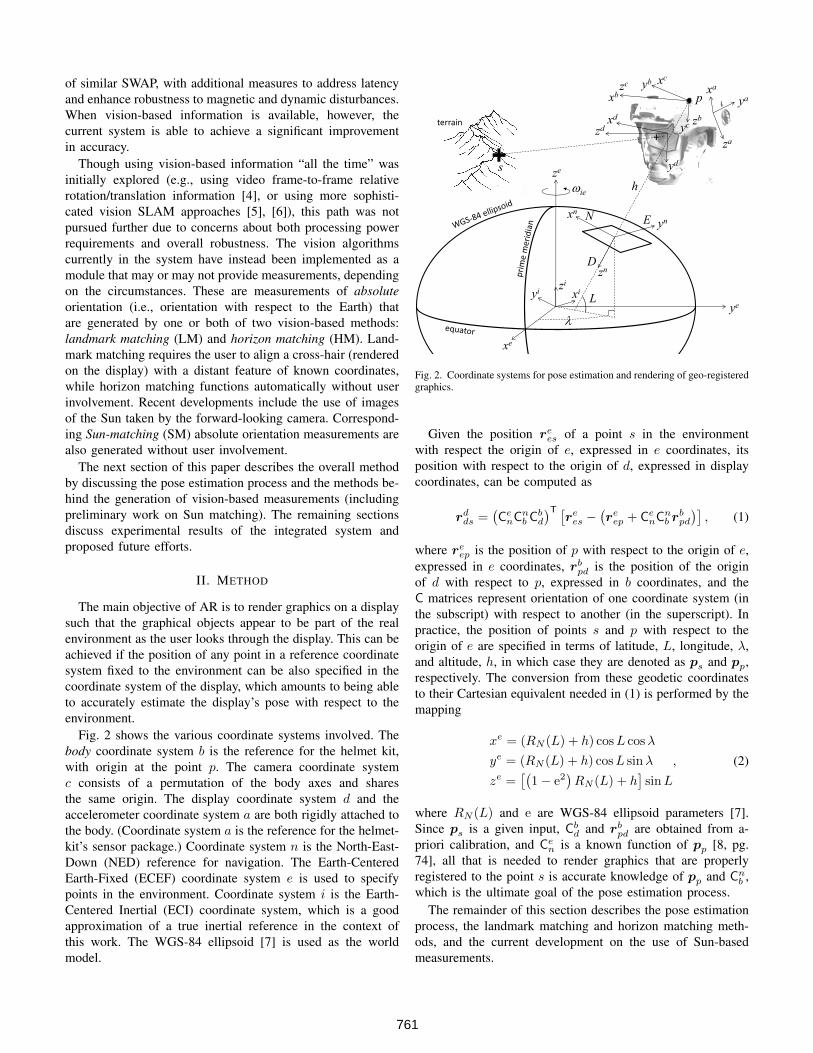
Fig. 2 shows the various coordinate systems involved. Thebody coordinate system b is the reference for the helmet kit,with origin at the point p. The camera coordinate systemc consists of a permutation of the body axes and sharesthe same origin. The display coordinate system d and theaccelerometer coordinate system a are both rigidly attached tothe body. (Coordinate system a is the reference for the helmet-kit’s sensor package.) Coordinate system n is the North-East-Down (NED) reference for navigation. The Earth-CenteredEarth-Fixed (ECEF) coordinate system e is used to specifypoints in the environment. Coordinate system i is the Earth-Centered Inertial (ECI) coordinate system, which is a goodapproximation of a true inertial reference in the context ofthis work. The WGS-84 ellipsoid [7] is used as the worldmodel.

L

l

h

xn

yn

zn

xe

ye

ze

N E

D

xb yb

zb

xi yi zi

wie

p

s

zd xd

yd

xa

za

ya

+ terrain

zc xc

yc

Fig. 2. Coordinate systems for pose estimation and rendering of geo-registeredgraphics.

Given the position rees of a point s in the environmentwith respect the origin of e, expressed in e coordinates, itsposition with respect to the origin of d, expressed in displaycoordinates, can be computed as

rdds =(CenCnb Cbd

)T [rees −

(reep + CenCnb r

bpd

)], (1)

where reep is the position of p with respect to the origin of e,expressed in e coordinates, rbpd is the position of the originof d with respect to p, expressed in b coordinates, and theC matrices represent orientation of one coordinate system (inthe subscript) with respect to another (in the superscript). Inpractice, the position of points s and p with respect to theorigin of e are specified in terms of latitude, L, longitude, λ,and altitude, h, in which case they are denoted as ps and pp,respectively. The conversion from these geodetic coordinatesto their Cartesian equivalent needed in (1) is performed by themapping

xe = (RN (L) + h) cosL cosλ

ye = (RN (L) + h) cosL sinλ

ze =[(

1− e2)RN (L) + h

]sinL

, (2)

where RN (L) and e are WGS-84 ellipsoid parameters [7].Since ps is a given input, Cbd and rbpd are obtained from a-priori calibration, and Cen is a known function of pp [8, pg.74], all that is needed to render graphics that are properlyregistered to the point s is accurate knowledge of pp and Cnb ,which is the ultimate goal of the pose estimation process.

The remainder of this section describes the pose estimationprocess, the landmark matching and horizon matching meth-ods, and the current development on the use of Sun-basedmeasurements.

761

A. Pose Estimation Process

The pose estimation framework consists of an ExtendedKalman Filter (EKF) implementation of a total-state loosely-coupled GPS/INS [8], designed to integrate additional aidingmeasurement of absolute orientation, without assumptionsabout their availability or periodicity. These “opportunistic”aiding measurements are provided by vision-based methods(LM and HM), which are described later. The main compo-nents and salient features of the pose estimation process arediscussed below.

1) Calibration: Helmet-kit hardware calibration consists ofestimating Cbd, rbpd, Cba, and rbpa. Estimation of the relativeorientation, Cba, of the sensor package with respect to thebody is performed by following the procedure in [9], whichalso yields an estimate of the camera’s intrinsic parameters.Estimation of the relative orientation, Cbd, of the display withrespect to the body is performed by an iterative process basedon using the current Cbd estimate to render scene features (e.g.,edges) from camera imagery onto the display, and adjusting ituntil the rendered features align with the corresponding actualscene features when viewed through the display. The positionvectors rbpd and rbpa can be obtained by straightforwardmeasurement, but in fact they are negligible in the context ofthis application (the former because ‖rpd‖ ‖rps‖, and thelatter because its magnitude is very small and was empiricallydetermined to have negligible effect). The magnetometer iscalibrated prior to each operation by following the proceduredescribed in [10].

2) EKF Models: The EKF is based on the model

x = f(x,u,w, t)

yk = hk(xk,νk),

where t is time, f is the continuous-time process, hk is thediscrete-time measurement (with output yk), x is the statevector, xk is its discrete-time equivalent, and u is the inputvector. The vector w is a continuous-time zero-mean white-noise process with covariance Q (denoted as w ∼ (0,Q)),and νk is a discrete-time zero-mean white-noise process withcovariance Rk (denoted as νk ∼ (0,Rk)).

The state is defined as x =[pp;v

nep; qnb; bg; ba; bα; bγ

](semicolons are used as row separators), where vnep is thevelocity of the point p with respect to the ECEF coordinatesystem, expressed in NED coordinates, and qnb is the quater-nion representation of Cnb . The vector bg is the rate gyro bias,ba is the accelerometer bias, and bα and bγ are biases in themodel of local magnetic declination and inclination values,respectively.

The rate gyro and accelerometer data are inputs to theprocess model, so that u = [ua;ug], with

ua = f bip + ba +wa

ug = ωbib + bg +wg

,

where f bip = CnbT[anep − gn + (ωnen + 2ωnie)× vnep

]is the

specific force at p, ωbib is the angular rate of the bodycoordinate system with respect to the ECI coordinate system,

wa ∼ (0,Qa), and wg ∼ (0,Qg). The cross product inthe f bip expression is a Coriolis and centripetal accelerationterm due to motion over the Earth’s surface [11], and can beneglected when the velocity is small (which is the case forpedestrian navigation).

Using the state definition and input model described above,the process model is specified by the following equations:

pp = fp (x) +wp

vnep = Cnb (ua − ba −wa) +

+gn − (ωnen + 2ωnie)× vnep +wv

qnb =1

2Ω (qnb)

(ug − bg −wg − ωbin

)+wq

bg = wbg

ba = wba

bα = wα

bγ = wγ

where fp is a known function of vnep, h, L, and WGS-84 parameters [8, pg. 61], gn is the acceleration due togravity, Ω is a 4×3 matrix that transforms an angular ratevector into the corresponding quaternion derivative [11, pg.44], and ωbin = Cnb

T (ωnie + ωnen). The process noise vec-tor is w =

[wp;wv;wq;wg;wbg ;wa;wba ;wα;wγ

], and

Q = blkdiag(Qp,Qv,Qq,Qg,Qbg ,Qa,Qba , σ

2α, σ

2γ

)is its

covariance matrix.The measurement vector is defined as

yk =

yLM

yHM

ya

ym

yGv

yGp

yD

=

qnb + νLM

qnb + νHM

CnbT(anep − gn

)+ ba + νa

CnbTmn + νm

vnep + νGv

pp + νGp

h+ νD

, (3)

where landmark matching, yLM, and horizon matching, yHM,are the vision-aiding measurements, ya is the accelerometermeasurement, ym is the magnetometer measurement, yGv

is the velocity measurement, yGp is the GPS horizontalposition (i.e., latitude and longitude) measurement, and yDis the measurement of altitude based on Digital Terrain andElevation Data (DTED). The measurement noise vector isνk = [νLM;νHM;νa;νm;νGv;νGp; νD], and its covariancematrix is Rk = blkdiag

(RLM,RHM,Ra,Rm,RGv,RGp, σ

2D

).

Because of the block-diagonal structure of Rk, the EKF mea-surement update step is executed by processing measurementsfrom each sensor as separate sequential updates (in the sameorder as they are listed in (3)).

The gravity vector is approximated as being perpendicularto the ellipsoid and therefore modeled as gn = [0; 0; g0(L)],where the down component g0(L) is obtained from theSomigliana model [7]. Note that since the acceleration anepis not directly measured nor modeled (accelerometers canonly measure specific force), it appears in (3) as an unknown

762

quantity that, when nonzero, has the effect of degrading thevalue of accelerometer measurements in aiding the estimate oforientation.

The reference magnetic field vector mn in (3) is the Earth’smagnetic field vector, expressed in n coordinates, and ismodeled as

mn =

cos(α− bα) cos(γ − bγ)

sin(α− bα) cos(γ − bγ)

sin(γ − bγ)

Bm, (4)

where Bm is the Earth’s magnetic field strength, and α andγ are the values of magnetic declination and inclination, re-spectively, obtained from the EMM2010 Earth magnetic model[12]. Because they are otherwise not observable, updating ofthe corresponding biases, bα and bγ , is only allowed when avision-aiding measurement is available.

3) Initialization and Alignment: The initial state x(0) isestimated by using sensor readings during the first few sec-onds of operation before the EKF process starts. The initialcondition of all biases is set to zero.

4) Parameter Tuning: Parameter tuning consists of estab-lishing values for Q, Rk, the initial estimated error covariancematrix P(0), and a number of parameters that are used fordisturbance detection, filtering, etc. This tuning has beenperformed by combining Allan variance analysis of sensordata [13], with the models described so far, to identify astarting point. Further adjustments were performed based onexperiments.

5) Dynamic Disturbance: Since they are used as measure-ments of the gravity vector in body coordinates, accelerometer-based updates are only valid if anep is zero (see (3)). If not,these measurements are considered to be corrupted by anunknown dynamic disturbance. The problem is addressed bydetecting the presence of this disturbance and, if detected,increasing the corresponding measurement noise covariancematrix, Ra, by a large factor ρa. Detection is based oncomparing the norm of the accelerometer measurement to‖gn‖, as well as checking that the measured angular rateis low enough. (The location of the sensor package on thehelmet kit, and the corresponding kinematics, result in angularrate being a very good indicator of anep.) The approach ofincreasing Ra implies that the unknown acceleration anep ismodeled as a stationary white noise process. Though the actualprocess is not stationary nor white, it was found experimentallythat this approach yields better results than the alternativeof completely rejecting accelerometer measurements that aredeemed disturbed. In fact, when testing this alternative, it wasobserved that a single valid measurement after long periodsof dynamic disturbance (as is the case when walking) couldcause undesirable jumps in the estimates of bg and ba, whileincreasing Ra resulted in no such issues.

6) Magnetic Disturbance: Magnetometer-based measure-ment updates are valid if the magnetic field being measuredis the Earth’s magnetic field only. Otherwise, these measure-ments are considered to be corrupted by an unknown mag-netic disturbance. The problem is addressed by detecting the

sensors DAQ Dt

vision processing

data xfer + EKF proc

camera DAQ

GPS/INS GPS/INS GPS/INS GPS/INS GPS/INS+ vision

GPS/INS

nav solution

Ns Dt

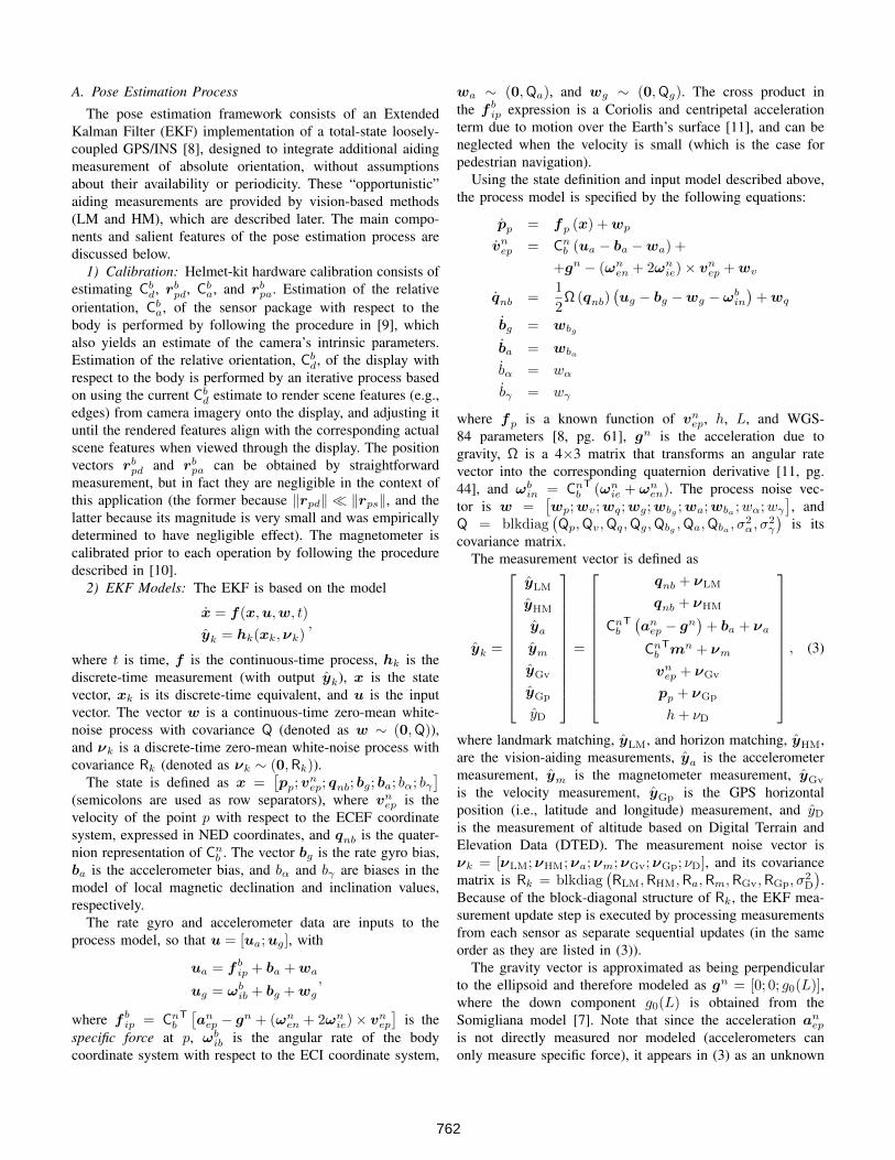
Fig. 3. Qualitative timing diagram of vision and EKF processing. Whenvision-based information is processed and delivered, the EKF must reprocesspast information. This extra processing is handled within a single EKF epoch∆t. Note that the image acquisition is synchronized with the sensor dataacquisition.

58.25 58.3 58.35 58.4 58.45

-129.3

-129.25

-129.2

-129.15

-129.1

-129.05

-129

Time (s)

Azim

uth

(deg)

HM measurement

LM measurement

Fig. 4. Vision-aiding measurement update. In the example illustrated by theinset, the EKF is able to “go back in time” and use the rewind buffer toreprocess the azimuth estimate based on the delayed HM measurement.

presence of magnetic disturbances and, if detected, rejectingthe corresponding magnetometer measurements. Detection isbased on comparing the norm of the measured magnetic fieldvector to the Earth’s field strength Bm, as well as checkingthat the computed inclination angle is not too far from thenominal value. (Since it is based on yT

mya, the latter check isonly performed if no dynamic disturbance is detected.)

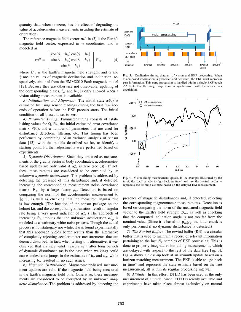
7) The Rewind Buffer: The rewind buffer (RB) is a circularbuffer that is used to maintain a record of relevant informationpertaining to the last Nr samples of EKF processing. This isdone to properly integrate vision-aiding measurements, whichare delayed with respect to the rest of the data (see Fig. 3).Fig. 4 shows a close-up look at an azimuth update based on ahorizon matching measurement. The EKF is able to “go backin time” and reprocess the state estimate based on the latemeasurement, all within its regular processing interval.

8) Altitude: In this effort, DTED has been used as the onlymeasurement of altitude. Since DTED is readily available andexperiments have taken place almost exclusively on natural

763

terrain, other options have not yet been explored. However,planned future tasks include integrating GPS and barometricaltitude measurements.

9) The Forward Buffer: The forward buffer (FB) is a bufferthat is used to store both the current state estimate x+

k andthe predicted state estimates up to Nf time steps ahead.That is, FBk =

x+k ,x

−k+1,x

−k+2, . . . ,x

−k+Nf

. Through

interpolation of the FB vectors, a state estimate can thenbe produced for any t ∈ [tk, tk +Nf∆t], where tk is thetime of the current estimate and ∆t is the EKF’s processinginterval. Given a value, ∆td, for system latency, the pose thatis delivered at time tk for rendering graphics on the displayis based on the predicted state at t = tk + ∆td, which isextracted from the FB. (Note that Nf must be selected suchthat Nf > 0 and Nf∆t ≥ ∆td.) The beneficial effect ofthis forward-prediction process is obvious when using thesystem, and focused experiments [2] have shown a reductionin perceived latency from about 40 ms to about 2 ms.

10) Adaptive Gyro Filtering: The forward-prediction pro-cess extrapolates motion to predict the state at some timein the future, and is inherently sensitive to noise. This mayresult in jitter of the rendered graphics even when the systemis perfectly stationary (e.g., mounted on a sturdy tripod).Low-pass filtering of the rate gyro signal, ug , reduces thisjitter effect but also introduces lag. Since this lag is notnoticeable when the rotation rate is near zero, and the jitteris not noticeable when there is actual motion, a reductionin perceived jitter is achieved by low-pass filtering the rategyro signal only when the estimated rotation rate magnitudeis small. This can be done by adjusting the low-pass filter’sbandwidth using a smooth increasing function of estimatedrotation rate magnitude. The resulting filtered signal can bethen used in place of ug in the EKF’s time-propagation steps(i.e., in the forward-prediction process). This method wasfound to reduce jitter by a factor of three without any adverseeffects in other performance measures [2].

11) Pose Estimation Processing Step: A single pose es-timation processing step takes as inputs the current sensordata, the RB data, and an index, inow, corresponding tothe current-time location in the RB. It returns updates toRB, inow, and the whole FB. It is implemented as fol-lows:

1: pre-process sensor data2: RB[inow]← sensor data, pre-processed data3: istop = inow4: if vision data is available and ∃ ivis : tCLK in RB[ivis] =tCLK in vision data then

5: inow = ivis6: end if7: keep processing = true8: while keep processing = true do9: x−,P− ← RB[inow]

10: RB[inow] ← x+,P+ = ekf u(x−,P−,RB[inow])11: inext = inow + 112: RB[inext] ← x−,P− = ekf p(x+,P+,RB[inow])

p

image plane

xb

yb

zb xc

yc

zc

e

ss

f

s s

+

ˆpsr

'psr

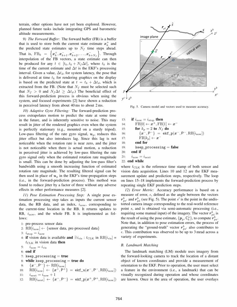
Fig. 5. Camera model and vectors used to measure accuracy.

13: if inow = istop then14: FB[0]← x+,FB[1]← x−

15: for kp = 2 to Nf do16: x−,P− = ekf p(x−,P−,RB[inow])17: FB[kp]← x−

18: end for19: keep processing = false20: end if21: inow = inext22: end whilewhere tCLK is the reference time stamp of both sensor andvision data acquisition. Lines 10 and 12 are the EKF mea-surement update and prediction steps, respectively. The loopon lines 15–18 implements the forward-prediction process byrepeating single EKF prediction steps.

12) Error Metric: Accuracy performance is based on ameasure of error, ε, defined as the angle between the vectorsrbps′ and rbps (see Fig. 5). The point s′ is the point in the undis-torted camera image corresponding to the real-world referencepoint s, and is obtained via semi-automatic processing (i.e.,requiring some manual input) of the imagery. The vector rbps isthe result of using the pose estimate, pp,Cnb , to compute rbps.Note that, in addition to pose estimation errors, the process ofgenerating the “ground-truth” vector rbps′ also contributes toε. This contribution was observed to be up to 3 mrad across avariety of experiments.

B. Landmark Matching

The landmark matching (LM) module uses imagery fromthe forward-looking camera to track the location of a distantobject of known coordinates and provide a measurement oforientation to the EKF. Prior to operation, the user must selecta feature in the environment (i.e., a landmark) that can bevisually recognized during operation and whose coordinatesare known. Once in the area of operation, the user overlays

764

a cross hair — rendered on the display and correspondingto the intersection of the camera’s optical axis with the imageplane (shown as a circle in Fig. 5) — on the selected landmarkand clicks a mouse button. This procedure is called “landmarkclicking”.

1) LM Method: Landmark clicking triggers the system toextract features from the current image and compute the cor-responding absolute orientation of the camera (and thereforethe body) using the known direction of the optical axis andthe EKF’s current estimate of roll angle. The combinationof extracted features and absolute orientation is stored in alandmark key-frame that can be compared to later imagesto determine their corresponding camera orientations. Fig. 6shows an illustration of the LM process in action. Once thelandmark key-frame is generated by the user, the LM moduleuses computer vision techniques to determine orientation.

Regarding the extraction of features in a given image,FAST [14] corners are extracted in the undistorted image andtheir BRIEF [15] descriptors are calculated. The tilt estimatefrom the EKF is then used to align the BRIEF descriptors withrespect to the down axis of the NED coordinate system. Thiseliminates the need for rotational invariance and increases thediscrimination power of the BRIEF descriptors compared tofeature descriptors, such as Oriented BRIEF (ORB) [16], thatuse image gradient information to orient the descriptors.

It is important to maintain robustness to the user walkingshort distances where the landmark is still in view aftermoving. Therefore, nearby image features, which move dueto parallax as the user walks, must be separated from farfeatures, which do not move. This can be done by a model-fitting approach consisting of fitting either an essential matrix[17], in the case where features are close, or a rotation matrixwhen all of the features are far away. In practice, it was foundthat in most cases features at intermediate distances exhibited asmall degree of parallax yet still fit a rotation-only hypothesismodel within the required accuracy. The small parallax in thesefeatures, however, was enough to create a bias in the rotationestimate and caused a corresponding orientation error to bepassed on to the EKF.

To alleviate this issue, a simple heuristic approach to featureselection was implemented, based on choosing only featuresthat are above a threshold distance from the camera. Thisdistance is computed using the EKF’s tilt estimate and theassumption of a flat ground in front of the camera. Ultimately,robustness of LM to translation depends on the user beingtrained to use it only for distant landmarks, without nearbyobjects in the scene to cause parallax. (Of course, the idealsituation for the current LM implementation is one where thecamera is not translating at all.)

After extraction, features in the current image are matchedto features in the landmark key-frame based on their BRIEFdescriptors, calculating the best matching feature as the onewith minimum Hamming distance. For each feature in thelandmark key-frame, its best match in the current image iscomputed. The same is done from the current image to thelandmark key-frame and only those matches that agree in both

directions are deemed valid. (This is a standard process ofcross-validation of feature matches.) After matching, a two-point RANSAC [18] procedure is applied to find the rotationbetween the two frames and eliminate outliers. Because thecamera has been calibrated, only the three degrees of freedomof the relative rotation between the landmark key-frame andcurrent images need to be estimated. Two feature matchesprovide four constraints and so over-constrain the solution.Each potential rotation solution is scored in the RANSACprocedure by rotating the current image’s features accordingto the inverse of the rotation and applying a threshold to thedistance to the corresponding feature matches in the landmarkframe. The number of feature matches satisfying the thresholdis the score for that solution.

Before delivering a measurement of orientation to the EKF,a few sanity checks must be satisfied. At least M featuresmatches are required between the landmark key-frame and thecurrent frame after RANSAC. This prevents incorrect rotationswith little support in the features from being passed to theEKF. The RANSAC procedure must also exceed a minimumtarget confidence in its solution. This confidence is calculatedas the probability p = 1− (1− is)n, where n is the number ofRANSAC iterations, s is the number of points selected at eachiteration, and i is the inlier ratio. (A lower bound of the trueinlier ratio can be computed by dividing the maximum numberof inliers that was observed by the total number of featurematches.) An upper bound on n is set to limit processing timeand meet real-time constraints, so it is possible that p may notreach the required level. The inlier ratios observed in practiceand the small number of points selected (i.e., s = 2) result ina high-enough p most of the time. A final check is that theangle between the optical axis of the landmark key-frame andthat of the current frame be less than twenty degrees, insuringadequate overlap between the two images.

A key feature of the LM method is that the object needsto be visible to the user but not necessarily to the camera.Since the LM module tracks FAST corner features around thelandmark object, these features need not be on the landmarkobject itself.

2) Standalone LM Results: Standalone results are producedby using the LM orientation measurement, yLM, to computeε, instead of using the EKF’s orientation estimate. The LMmodule has been tested in a variety of environments to verifythe generality of its algorithms. One example is an area ofthe Smoky Mountains (see images in Fig. 9), characterizedby green, tree-covered, rounded mountains, as well as plentyof vegetation in the lower flatter areas. Another exampleis the area around Red Rock Canyon, NV (see images inFig. 6), characterized by desert-like landscape, with rocksand bushes in the flat areas, and sharp, bare-rock mountainpeaks. A sample of performance of the LM module in theseenvironments is shown in plots (a) of Fig. 7 and Fig. 8.LM performed well in both cases, with a mean error lessthan 3 mrad. Because the landmark is designated by the user,and can only be matched when it is in the field of view ofthe camera, only limited sections of the data have landmark

765

(a) (b) (c)

(d) (e) (f)

t = 70 m < M d = 0 y = -128 t = 96 m < M d = 0 y = -92 t = 104 m = 49 d = 0 y = -127

t = 146 m = 38 d = 22 y = -125 t = 169 m = 30 d = 48 y = -131 t = 185 m < M d = 62 y = -128

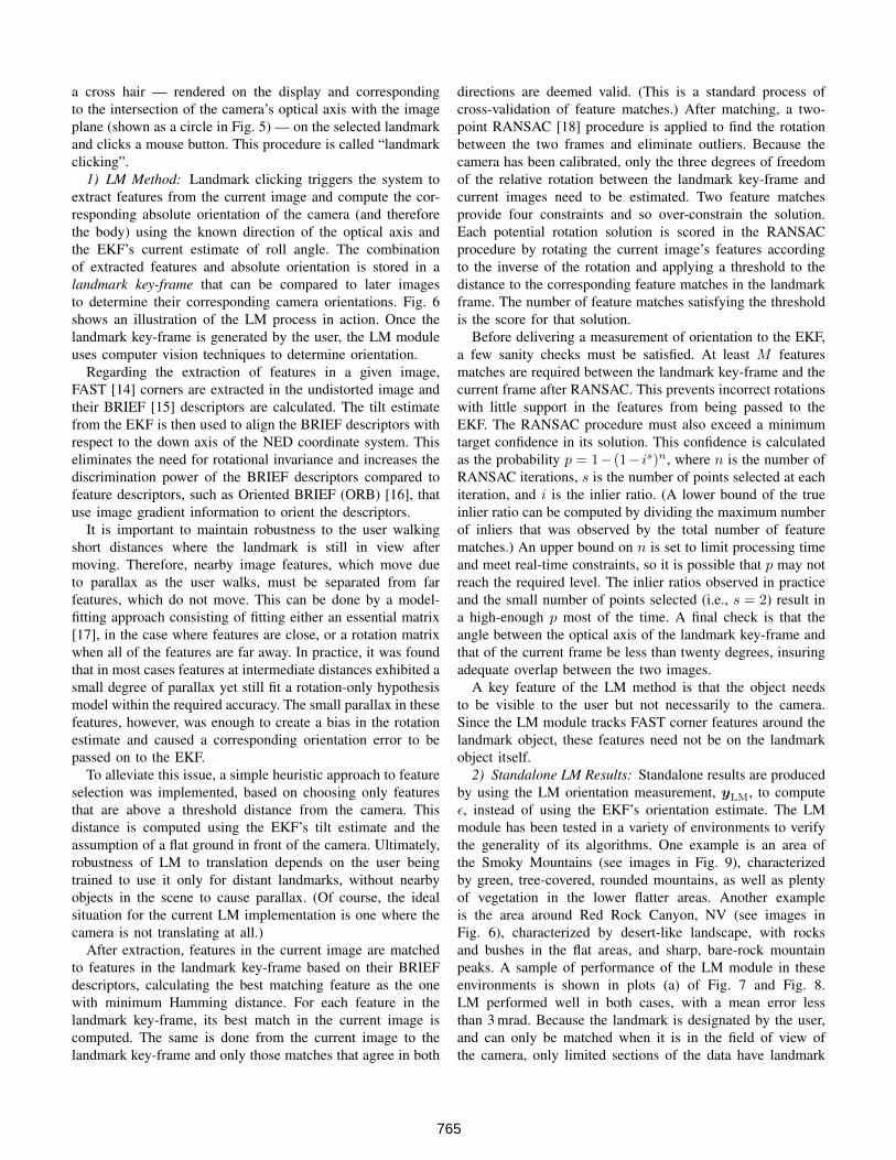
Fig. 6. Illustration of the landmark matching process using imagery from the forward-looking camera. The small cross hair in each image corresponds to thecamera’s optical axis and is used to align the camera to the known landmark. Image (a) shows the moment when the landmark (the mountain peak shown inthe inset and by the large arrow) is clicked, generating a landmark key-frame. In image (b) the user has looked away from the landmark and there are notenough feature matches. In image (c) the user looks back at the landmark and the software automatically re-acquired the landmark by matching m = 49features (shown by circles) to the landmark key-frame. The user then walks 22 m (d) and 48 m (e) from the starting point and the landmark is re-acquiredin each case. Image (f) shows that after walking 62 meters the landmark is not re-acquired. Each image is annotated with the elapsed time t in seconds, thenumber of matched features m, the distance d from the starting point in meters, and the estimated azimuth ψ in degrees. M is the minimum number ofmatches that are required (in this case, M = 20).

measurements, and those sections typically correspond tostationary conditions (i.e., not walking). Overall, when the userrequires it, landmark matching can provide a highly accurateorientation measurement.

C. Horizon Matching

The horizon matching (HM) module provides a measure-ment of absolute orientation by comparing edges detected inthe camera imagery with a horizon silhouette edge generatedfrom DTED, using a hierarchical search algorithm initializedat the current orientation estimate from the EKF.

Stein and Medioni [19] demonstrated feasibility of local-ization from horizon data using fully synthetic experiments.Their method approximated the horizon as a set of linesegments and employed several line-fitting tolerances duringthe matching. In contrast to Stein and Medioni, the methoddescribed here uses real-world data and can generate refinedorientation measurements at 20 Hz with current hardware.Behringer et al. [20] estimate camera pose by comparingsalient points in a horizon silhouette derived from DTED tothe visible horizon silhouette extracted from the camera image.The assumption is made that the horizon silhouette showsup as a strong-gradient edge in the image, which is not thecase under various lighting conditions and in cases of severeocclusions by foreground objects. The method described hereis robust to both of these disturbances because it uses only

the more stable parts of the horizon. More recently, Badoudet al. [21] proposed a robust system for pose estimationthat finds the best alignment between a 3D terrain model andan input image. An interesting aspect of their system is thatthey leveraged secondary silhouettes (visible local mountainpeaks or ridges that do not coincide with the uppermostvisible horizon silhouette) in the terrain data and the imageto improve their alignment. They were able to achieve veryaccurate results over various types of mountainous terrain, buttheir system is far too computationally expensive, preventingits use in real-time low-SWAP applications.

1) HM Method: The basic principle of the HM methodpresented here is that given the user’s position and a 3Dheight map of the terrain surrounding him, a corresponding360-degree horizon can be computed. If accurate alignmentcan be found between the computed horizon and the horizonextracted from the camera imagery, then the camera’s absoluteorientation can be determined.

After transforming the DTED into ECEF coordinates, thenext step is to determine the corresponding shape of the hori-zon from the user’s estimated current position. This 3D terrainmodel is then rendered onto a unit sphere centered at the user’sposition, where the rendering resolution is chosen to matchthe native resolution of the camera. To support automaticextraction of the horizon silhouette, the 3D terrain model isrendered as a white surface onto a black background, so that

766

0 50 100 150 200 250 300 350 4000

5

10

15

20

Angula

r E

rror,

(

mra

d)

0 50 100 150 200 250 300 350 4000

5

10

15

20

Angula

r E

rror,

(

mra

d)

0 50 100 150 200 250 300 350 4000

5

10

15

20

Accele

ration (

m/s

2)

0 50 100 150 200 250 300 350 4000

100

200

300

Time (s)

Angula

r R

ate

(deg/s

)

(a)

(c)

(b)

(d)

LM

HM 126.5 46.1

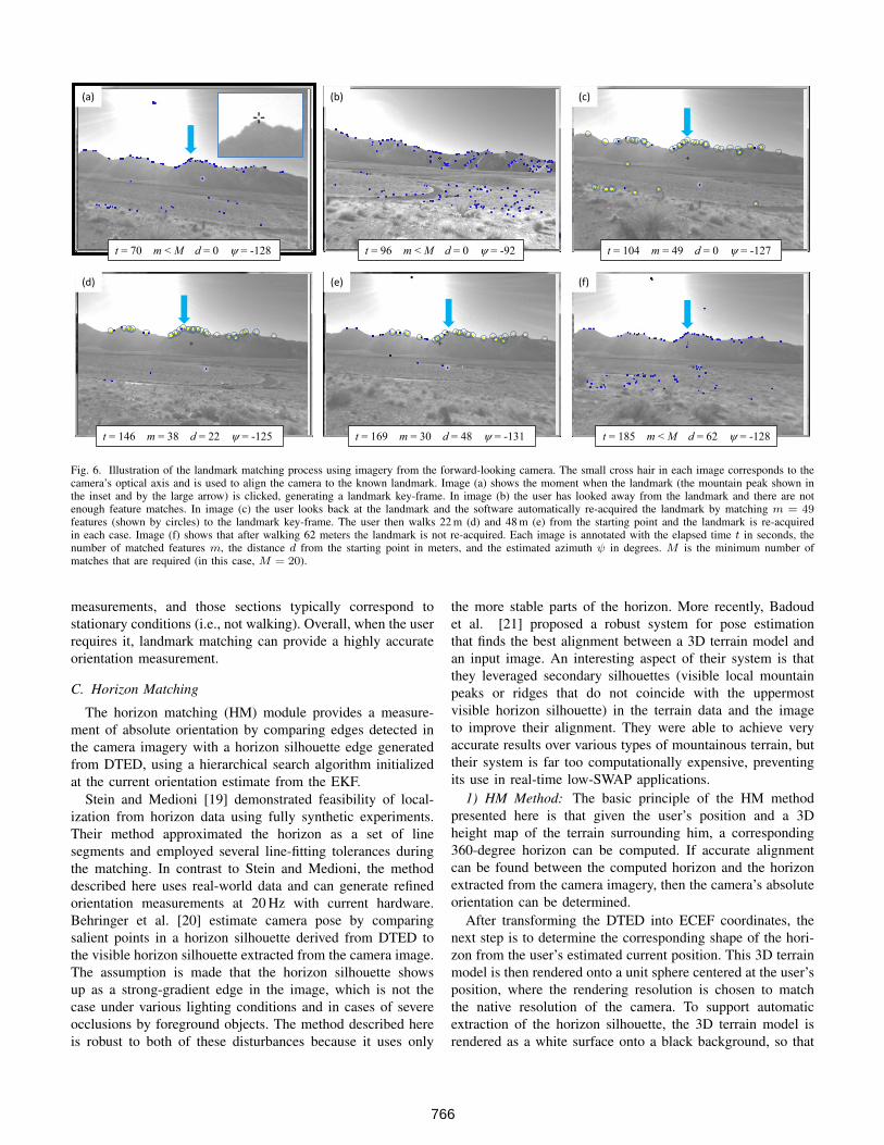
Fig. 7. Sample standalone accuracy performance (as defined in Sec. II-A12) of the LM module (a) and HM module (b) during field tests in the SmokyMountains. Plots (c) and (d) show the accelerometer and rate gyro data, respectively, to give an indication of dynamic conditions. In this sample, LM has amean error of 2.9 mrad with a standard deviation of 1.0 mrad. Note that LM is used under stationary conditions (i.e., not walking), when needed by the user.The HM module, on the other hand, functions automatically and produces a measurement as long as there is a horizon available to match. Note, however, thepresence of two false positive matches (outliers) in plot (b). In this sample, without including the outliers, HM has a mean error of 4.3 mrad with a standarddeviation of 2.6 mrad.

the horizon extraction becomes a simple edge detection. Usingthe inverse of the camera calibration matrix, each pixel alongthe horizon is converted to its corresponding image vector, andnormalizing these vectors yields a spherical representation ofthe horizon silhouette.

Given the spherical representation of the horizon silhouette,several optimizations can be performed to improve the compu-tational efficiency. To facilitate data compression and improveprocessing efficiency, a continuous connected chain is createdthat represents the 360-degree horizon silhouette. First, edgesare extracted from the projected spherical image followed byan edge-following algorithm in the image to define an edgechain. While the edge chain is a very good representationof the horizon, it is also a very dense representation posingcomputational challenges for the alignment. This leads to asecond step in which the pixel-resolution chain is reduced to amuch smaller set of line segments that satisify a maximum tan-gential distance. The resulting piece-wise linear representationtypically reduces the complexity of the horizon and greatlyboosts the computational efficiency.

To extract a horizon from the camera imagery, edge detec-tion is performed on each undistorted image by first blurringwith a Gaussian filter and then using a Sobel filter along both

the horizontal and vertical directions. From this, the squarededge response is computed at each pixel location by summingthe squares of the vertical and horizontal edge components.Then the image of the squared edge response is blurred againwith a Gaussian filter to effectively increase the size of theedges. The last step is to threshold the edge response so thatit is equal to one along the edges and zero elsewhere. Thethreshold is set so that the resulting edges are around five toten pixels wide (the advantage of which is discussed later).At this point in the process, a pyramidal representation ofedge images is also created, which is used later in a course-to-fine search. To create the down-sampled images, a simplebilinear interpolation scheme is applied where the results arethen rounded to maintain the binary nature of the edge image.The rationale for this process is that extracting the edges fromthe imagery is desirable because the actual horizon silhouetteis typically an edge within the image. The reason for thethresholding is that in many cases, the strength of the edgealong the horizon varies, even within the same frame-to-framevideo sequence. The desired approach is to treat a strong edgein the same manner as a weak edge, as each are equally aslikely to be the true horizon silhouette.

The next step is to perform an optimization that seeks

767

0 50 100 150 200 250 300 350 4000

5

10

15

20

Angula

r E

rror,

(

mra

d)

0 50 100 150 200 250 300 350 4000

5

10

15

20

Angula

r E

rror,

(

mra

d)

0 50 100 150 200 250 300 350 4000

10

20

30

Accele

ration (

m/s

2)

0 50 100 150 200 250 300 350 4000

100

200

300

Time (s)

Angula

r R

ate

(deg/s

)

(a)

(c)

(b)

(d)

LM, SM

HM

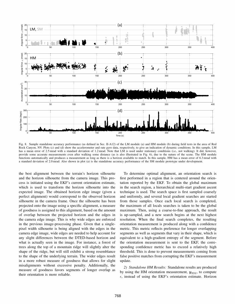
Fig. 8. Sample standalone accuracy performance (as defined in Sec. II-A12) of the LM module (a) and HM module (b) during field tests in the area of RedRock Canyon, NV. Plots (c) and (d) show the accelerometer and rate gyro data, respectively, to give an indication of dynamic conditions. In this sample, LMhas a mean error of 2.5 mrad with a standard deviation of 1.2 mrad. Note that LM is used under stationary conditions (i.e., not walking). It did, however,provide some accurate measurements even after walking some distance (as is also illustrated in Fig. 6), due to the nature of the scene. The HM modulefunctions automatically and produces a measurement as long as there is a horizon available to match. In this sample, HM has a mean error of 6.3 mrad witha standard deviation of 2.0 mrad. Also shown in plot (a) is the standalone accuracy performance of the SM module prototype under development.

the best alignment between the terrain’s horizon silhouetteand the horizon silhouette from the camera image. This pro-cess is initiated using the EKF’s current orientation estimate,which is used to transform the horizon silhouette into theexpected image. The obtained horizon edge image (given aperfect alignment) would correspond to the observed horizonsilhouette in the camera frame. Once the silhouette has beenprojected onto the image using a specific alignment, a measureof goodness is assigned to this alignment, based on the amountof overlap between the projected horizon and the edges inthe camera edge image. This is why wide edges are enforcedin the previous image-processing phase. Given that a single-pixel width silhouette is being aligned with the edges in thecamera edge image, wide edges are needed to help account forany slight differences between the DTED-based horizon andwhat is actually seen in the image. For instance, a forest oftrees along the top of a mountain ridge will slightly alter theshape of the ridge, but will still exhibit a strong resemblanceto the shape of the underlying terrain. The wider edges resultin a more robust measure of goodness that allows for slightmisalignments without excessive penalty. Additionally, themeasure of goodness favors segments of longer overlap astheir orientation is more reliable.

To determine optimal alignment, an orientation search isfirst performed in a region that is centered around the orien-tation reported by the EKF. To obtain the global maximumin the search region, a hierarchical multi-start gradient ascenttechnique is used. The search space is first sampled coarselyand uniformly, and several local gradient searches are startedfrom those samples. Once each local search is completed,the maximum of all locals searches is taken to be the globalmaximum. Then, using a coarse-to-fine approach, the resultis up-sampled, and a new search begins at the next highestresolution. When the final search completes, the resultingorientation measurement is produced along with a confidencemetric. This metric reflects preference for longer overlappingsegments as well as segments that vary in their shape, which isequivalent to a high-gradient entropy of the segment. Beforethe orientation measurement is sent to the EKF, the corre-sponding confidence metric has to exceed a relatively highthreshold. This is done to prevent measurements coming fromfalse positive matches from corrupting the EKF’s measurementupdate.

2) Standalone HM Results: Standalone results are producedby using the HM orientation measurement, yHM, to computeε, instead of using the EKF’s orientation estimate. Horizon

768

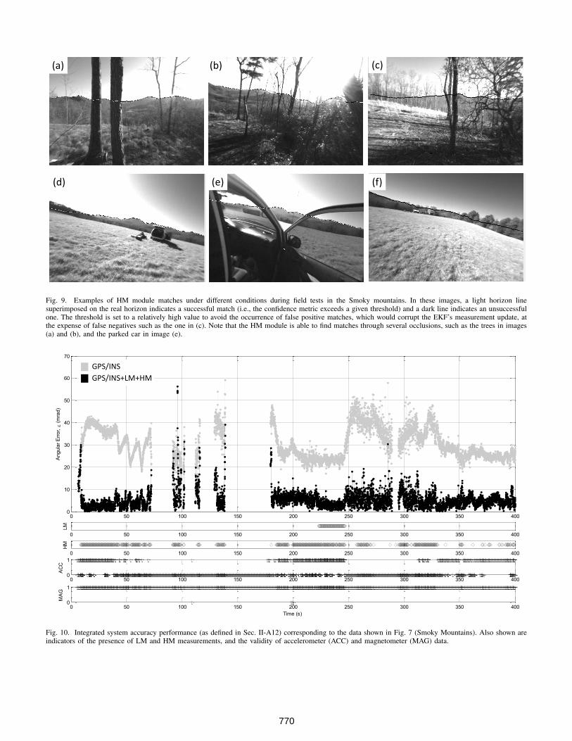
matching typically works best in mountainous environmentsbecause of the distinctiveness of the horizon’s shape. The HMmodule was tested in multiple distinctly different mountainousregions including the Smoky Mountains (see Fig. 9) and RedRock Canyon, NV (see Fig. 6), and was able to tolerate thelarge differences in horizon shapes. A sample of performanceof the HM module in these environments is shown in plots (b)of of Fig. 7 and Fig. 8. HM performed well in both cases, witha mean error less than 7 mrad. Note in Fig. 7 that there area couple of outliers corresponding to false positives whoseconfidence metric passed the threshold test. These have thepotential of affecting the integrated solution (the effect of thefirst of the two false positives is obvious as a spike in theerror plot of Fig. 10). Though not yet implemented, theseisolated outliers could be detected in the EKF by monitoringthe statistics of zHM = yHM − yHM. On the plus side, notein Fig. 9 that the HM module is able to find matches throughseveral occlusions, such as the trees in images (a) and (b),and the parked car in image (e). Overall, when a reasonablydistinctive horizon is in view, horizon matching can providean accurate and robust orientation measurement.

D. Sun Matching

After a recent field test, it was noticed that the Sun appearedin a large portion of the camera imagery as a black spot on anotherwise bright sky (see, for example, image (e) of Fig. 6).In fact, this “eclipsing” phenomenon is characteristic of manyCMOS sensors and occurs when the photo-generated chargeof a pixel is so large that it impacts the pixel’s reset voltageand subsequently the signal-reset difference level presentedto the analog-to-digital converter. This results in saturatedpixels being incorrectly decoded as dark pixels. Most CMOSsensors include anti-eclipse circuitry to minimize this effect,but this function had been effectively disabled in our camera.The resulting black-Sun artifact prompted an exploration ofSun-based measurements of orientation, and a preliminarySM module was developed that uses the Sun’s location inthe camera image to generate a measurement of the camera’sabsolute orientation.

1) SM Method: The basic method consists of the followingsteps:

1: find pixel coordinates of black-Sun centroid in undistortedcamera image

2: convert pixel coordinates into measured Sun vector in bcoordinates, sb

3: compute reference Sun vector in n coordinates, sn

4: using EKF’s roll estimate as constraint, find Cnb such thatCnb s

b = sn

The camera model shown in Fig. 5 is used in line 2. Inline 3, using an astronomical model [22] and knowledge ofpp, date, and time, the reference Sun vector is computedas azimuth and zenith angles in the n coordinate system.The Sun-based orientation estimate returned to the EKF isthe rotation matrix that aligns the reference Sun vector in ncoordinates with the measured Sun vector in b coordinates,as shown in line 4. This requirement only constrains two out

of three angular degrees of freedom, so a third constraint isimposed, which is that the roll angle represented in the Sun-based orientation estimate must be the same as the one inthe current EKF estimate of orientation. Under this constraint,a gradient-descent optimization method is used to find therotation matrix Cnb that most closely satisfies Cnb s

b = sn.2) Standalone SM Results: Standalone results are produced

by using the SM orientation measurement to compute ε,instead of using the EKF’s orientation estimate. Since theSun matching method is still under development, it is not yetintegrated into the system for real-time operation. Therefore,sample results were obtained by post-processing GPS/INSdata corresponding to the sample experiment of Fig. 8. TheGPS/INS solution in that experiment was used to provide ppand a roll estimate to the SM algorithm. The resulting outputof the SM module is shown in plot (a) of Fig. 8, where theaccuracy performance is shown to be similar to that of LMwhen the user is stationary. As the user walks, performancedegrades but is still shown to be better than GPS/INS alone.This degradation may be caused by errors in the GPS/INSestimate of roll being propagated to the SM solution.

Being based on a single data collect and a first-try algo-rithm, these results are very preliminary. Further developmentwill include exploring different algorithm options (especiallyregarding other choices of enforced constraint) and testing in avariety of environments and sky conditions. Optimum cameraplacement and field-of-view strategies must also be evaluatedand the robustness of the CMOS sensor’s eclipse feature mustbe determined. At this point, however, it is already clear thatSun-based pose estimates are a promising opportunistic aid tonavigation solutions.

III. INTEGRATED SYSTEM RESULTS

All results presented in this paper are based on real-timepose estimation data collected with the actual system duringfield tests in unprepared outdoor environments. The corre-sponding computer hardware consists of an off-the-shelf em-bedded processing module (SECO QuadMo747-X/T30) withan Nvidia Tegra 3 system-on-chip (SoC) and 2 GB of DDR3Lmemory on-board. This computing hardware uses about 12 Wof power at full load provided by a high-capacity battery, andruns a standard version of Ubuntu Linux 12.04 provided bySECO, which supports “hard-float” binary modules.

Accuracy performance results were shown for the individualvision-aiding measurement modules in Fig. 7 and Fig. 8. Inthis section, integrated system (i.e., vision-aided) accuracyperformance results based on the same two representative datasets is discussed. These results, shown in Fig. 10 and Fig. 11,correspond to system operation of several minutes under avarious dynamic and magnetic conditions. Also shown in thesefigures are indicators of the presence of LM and HM aidingmeasurements, and the validity of accelerometer (ACC) andmagnetometer (MAG) data (based on previously discusseddynamic and magnetic disturbance detection).

Both Fig. 10 and Fig. 11 show the GPS/INS-only (i.e., novision-aiding) solution performance varying about an offset of

769

(a) (b) (c)

(d) (e) (f)

Fig. 9. Examples of HM module matches under different conditions during field tests in the Smoky mountains. In these images, a light horizon linesuperimposed on the real horizon indicates a successful match (i.e., the confidence metric exceeds a given threshold) and a dark line indicates an unsuccessfulone. The threshold is set to a relatively high value to avoid the occurrence of false positive matches, which would corrupt the EKF’s measurement update, atthe expense of false negatives such as the one in (c). Note that the HM module is able to find matches through several occlusions, such as the trees in images(a) and (b), and the parked car in image (e).

0 50 100 150 200 250 300 350 4000

10

20

30

40

50

60

70

Angula

r E

rror,

(

mra

d)

0 50 100 150 200 250 300 350 400

LM

0 50 100 150 200 250 300 350 400

HM

0 50 100 150 200 250 300 350 4000

1

AC

C

0 50 100 150 200 250 300 350 4000

1

Time (s)

MA

G

GPS/INS

GPS/INS+LM+HM

Fig. 10. Integrated system accuracy performance (as defined in Sec. II-A12) corresponding to the data shown in Fig. 7 (Smoky Mountains). Also shown areindicators of the presence of LM and HM measurements, and the validity of accelerometer (ACC) and magnetometer (MAG) data.

770

0 50 100 150 200 250 300 350 4000

10

20

30

40

50

60

70A

ngula

r E

rror,

(

mra

d)

0 50 100 150 200 250 300 350 400

LM

0 50 100 150 200 250 300 350 400

HM

0 50 100 150 200 250 300 350 4000

1

AC

C

0 50 100 150 200 250 300 350 4000

1

Time (s)

MA

G

GPS/INS

GPS/INS+LM+HM

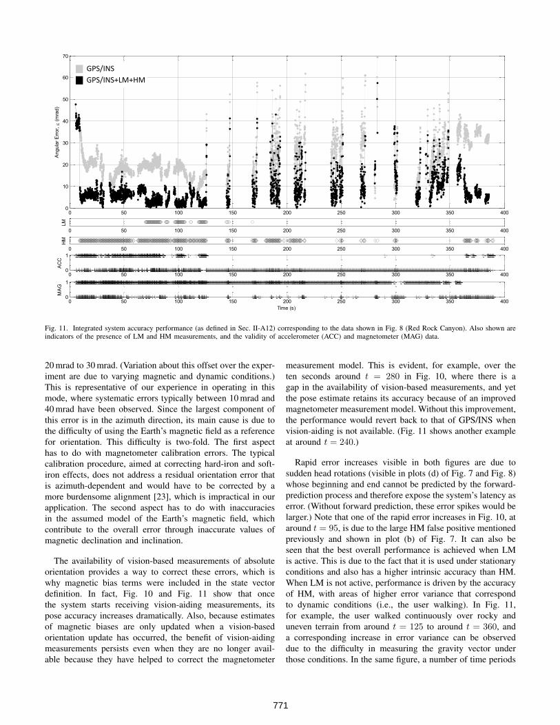
Fig. 11. Integrated system accuracy performance (as defined in Sec. II-A12) corresponding to the data shown in Fig. 8 (Red Rock Canyon). Also shown areindicators of the presence of LM and HM measurements, and the validity of accelerometer (ACC) and magnetometer (MAG) data.

20 mrad to 30 mrad. (Variation about this offset over the exper-iment are due to varying magnetic and dynamic conditions.)This is representative of our experience in operating in thismode, where systematic errors typically between 10 mrad and40 mrad have been observed. Since the largest component ofthis error is in the azimuth direction, its main cause is due tothe difficulty of using the Earth’s magnetic field as a referencefor orientation. This difficulty is two-fold. The first aspecthas to do with magnetometer calibration errors. The typicalcalibration procedure, aimed at correcting hard-iron and soft-iron effects, does not address a residual orientation error thatis azimuth-dependent and would have to be corrected by amore burdensome alignment [23], which is impractical in ourapplication. The second aspect has to do with inaccuraciesin the assumed model of the Earth’s magnetic field, whichcontribute to the overall error through inaccurate values ofmagnetic declination and inclination.

The availability of vision-based measurements of absoluteorientation provides a way to correct these errors, which iswhy magnetic bias terms were included in the state vectordefinition. In fact, Fig. 10 and Fig. 11 show that oncethe system starts receiving vision-aiding measurements, itspose accuracy increases dramatically. Also, because estimatesof magnetic biases are only updated when a vision-basedorientation update has occurred, the benefit of vision-aidingmeasurements persists even when they are no longer avail-able because they have helped to correct the magnetometer

measurement model. This is evident, for example, over theten seconds around t = 280 in Fig. 10, where there is agap in the availability of vision-based measurements, and yetthe pose estimate retains its accuracy because of an improvedmagnetometer measurement model. Without this improvement,the performance would revert back to that of GPS/INS whenvision-aiding is not available. (Fig. 11 shows another exampleat around t = 240.)

Rapid error increases visible in both figures are due tosudden head rotations (visible in plots (d) of Fig. 7 and Fig. 8)whose beginning and end cannot be predicted by the forward-prediction process and therefore expose the system’s latency aserror. (Without forward prediction, these error spikes would belarger.) Note that one of the rapid error increases in Fig. 10, ataround t = 95, is due to the large HM false positive mentionedpreviously and shown in plot (b) of Fig. 7. It can also beseen that the best overall performance is achieved when LMis active. This is due to the fact that it is used under stationaryconditions and also has a higher intrinsic accuracy than HM.When LM is not active, performance is driven by the accuracyof HM, with areas of higher error variance that correspondto dynamic conditions (i.e., the user walking). In Fig. 11,for example, the user walked continuously over rocky anduneven terrain from around t = 125 to around t = 360, anda corresponding increase in error variance can be observeddue to the difficulty in measuring the gravity vector underthose conditions. In the same figure, a number of time periods

771

with magnetic disturbance can also be observed. Overall, sincethe performance shown in these figures is representative ofwhat was observed across many other field tests, this vision-aided navigation system consistently showed a significantimprovement over the GPS/INS solution, maintaining a meanerror below 10 mrad over a wide range of magnetic and/ordynamic conditions.

Exploiting signals of opportunity such as the vision-basedmeasurements described in this paper is a sensible and feasiblestrategy for greatly expanding the operational envelope ofhigh-accuracy, low-SWAP navigation systems. It is a promis-ing path toward achieving the “Holy Grail” of robust andaccurate tracking outdoors, for augmented reality everywhere.

IV. FUTURE WORK

Opportunities for future work consist of continuing explo-rations that were started but left at the preliminary stage, aswell as undertaking new investigations based on what waslearned during the development of the current system. Theseinclude:• Integration of other available altitude measurements;• Revisiting tight integration of frame-to-frame vision in-

formation;• Revisiting the possible role and use of vision-based

SLAM techniques;• Development and implementation of enhanced magne-

tometer calibration;• Development and implementation of enhanced magnetic

measurement error model to provide a means of updatingthe magnetometer calibration in real-time when absoluteorientation measurements are available;

• Continuation of SM investigation and development;• Continued enhancement of LM and HM algorithms aimed

at improving robustness and providing an appropriatemeasure of uncertainty and/or integrity of the correspond-ing measurements;

• Development and implementation of enhanced integritymonitoring, to provide timely warning of degraded per-formance to the user and generate appropriate measuresof uncertainty in the state estimate.

Plans for future work also include integrating all of thecurrent software onto the Android platform. Newer processorarchitectures are also being tested and preliminary resultssuggest major performance gains.

ACKNOWLEDGMENT

This research was funded by the DARPA ULTRA-Visprogram under AFRL contract FA8650-09-C-7909 as well asARA internal research and development investment. The viewsexpressed in this paper are those of the authors and do notreflect the official policy or position of the Department ofDefense or the U.S. Government.

REFERENCES

[1] G. F. Welch, “History: The use of the kalman filter for human motiontracking in virtual reality,” Presence, vol. 18, no. 1, pp. 72–91, 2009.

[2] D. Roberts, A. Menozzi, J. Cook, T. Sherrill, S. Snarski, P. Russler,B. Clipp, R. Karl, E. Wenger, M. Bennett et al., “Testing and evaluationof a wearable augmented reality system for natural outdoor environ-ments,” in SPIE Defense, Security, and Sensing, 2013, pp. 87 350A1–87 350A16.

[3] P. Corke, J. Lobo, and J. Dias, “An introduction to inertial and visualsensing,” The International Journal of Robotics Research, vol. 26, no. 6,pp. 519–535, 2007.

[4] A. I. Mourikis, S. I. Roumeliotis, and J. W. Burdick, “Sc-kf mobile robotlocalization: A stochastic cloning kalman filter for processing relative-state measurements,” IEEE Transactions on Robotics, vol. 23, no. 4, pp.717–730, 2007.

[5] A. J. Davison, I. D. Reid, N. D. Molton, and O. Stasse, “Monoslam:real-time single camera slam,” IEEE transactions on pattern analysisand machine intelligence, vol. 29, no. 6, pp. 1052–1067, 2007.

[6] T. Lemaire, C. Berger, I.-K. Jung, and S. Lacroix, “Vision-based slam:Stereo and monocular approaches,” International Journal of ComputerVision, vol. 74, no. 3, pp. 343–364, 2007.

[7] National Imagery and Mapping Agency, “Nga: Dod worldgeodetic system 1984: Its definition and relationships withlocal geodetic systems.” [Online]. Available: http://earth-info.nga.mil/GandG/publications/tr8350.2/wgs84fin.pdf

[8] P. D. Groves, Principles of GNSS, inertial, and multisensor integratednavigation systems, 2nd ed., ser. GNSS technology and applicationseries. Boston: Artech House, 2013.

[9] J. Lobo and J. Dias, “Relative pose calibration between visual and in-ertial sensors,” The International Journal of Robotics Research, vol. 26,no. 6, pp. 561–575, 2007.

[10] T. Ozyagcilar, “Calibrating an ecompass in the presenceof hard and soft-iron interference,” 2013. [Online]. Available:http://www.freescale.com/files/sensors/doc/app note/AN4246.pdf

[11] D. H. Titterton, Strapdown Inertial Navigation Technology, 2nd ed.AIAA, 2004.

[12] S. Maus, “An ellipsoidal harmonic representation of earth’s lithosphericmagnetic field to degree and order 720,” Geochemistry, Geophysics,Geosystems, vol. 11, no. 6, pp. 1–12, 2010.

[13] Gyro and Accelerometer Panel of the IEEE Aerospace and ElectronicSystem s Society, “Ieee std 952-1997, ieee standard specification formatguide and test pro cedure for single-axis interferometric fiber opticgyros,” 2008.

[14] E. Rosten and T. Drummond, “Machine learning for high-speed cornerdetection,” Computer Vision–ECCV 2006, pp. 430–443, 2006.

[15] M. Calonder, V. Lepetit, M. Ozuysal, T. Trzcinski, C. Strecha, andP. Fua, “Brief: Computing a local binary descriptor very fast,” IEEETransactions on Pattern Analysis and Machine Intelligence, vol. 34,no. 7, pp. 1281–1298, 2012.

[16] E. Rublee, V. Rabaud, K. Konolige, and G. Bradski, “Orb: An efficientalternative to sift or surf,” in Computer Vision (ICCV), 2011 IEEEInternational Conference on, Nov 2011, pp. 2564–2571.

[17] R. I. Hartley and A. Zisserman, Multiple View Geometry in ComputerVision, 2nd ed. Cambridge University Press, ISBN: 0521540518, 2004.

[18] M. A. Fischler and R. C. Bolles, “Random sample consensus: Aparadigm for model fitting with applications to image analysis andautomated cartography,” Communications of the ACM, vol. 24, no. 6,May 1981.

[19] F. Stein and G. Medioni, “Map-based localization using the panoramichorizon,” in Proceedings of the IEEE International Conference onRobotics and Automation, 1992.

[20] R. Behringer, “Improving the registration precision by visual horizonsilhouette matching,” Proceedings of the First IEEE Workshop onAugmented Reality, 1998.

[21] L. Baboud, M. Cadik, E. Eisemann, and H.-P. Seidel, “Automatic photo-to-terrain alignment for the annotation of mountain pictures,” ComputerVision and Pattern Recognition (CVPR), 2011 IEEE Conference on DOI- 10.1109/CVPR.2011.5995727, pp. 41–48, 2011.

[22] I. Reda and A. Andreas, “Solar position algorithm for solar radiationapplications,” Solar energy, vol. 76, no. 5, pp. 577–589, 2004.

[23] J. F. Vasconcelos, G. Elkaim, C. Silvestre, P. Oliveira, and B. Cardeira,“Geometric approach to strapdown magnetometer calibration in sen-sor frame,” IEEE Transactions on Aerospace and Electronic Systems,vol. 47, no. 2, pp. 1293–1306, 2011.

772