Development of Unified High-Fidelity Flight Dynamic

Research ArticleDevelopment of Unified High-Fidelity Flight Dynamic ModelingTechnique for Unmanned Compound Aircraft

Do hyeon Lee,1 Chang-joo Kim ,2 and Seong han Lee3

1Turret Technology Team, Hanwha Defense, Seongnam-si 13488, Republic of Korea2Konkuk University, Seoul 05029, Republic of Korea3Avionics System Team, Hanwha System, Seongnam-si 13524, Republic of Korea

Correspondence should be addressed to Chang-joo Kim; [email protected]

Received 23 February 2021; Revised 14 April 2021; Accepted 19 April 2021; Published 4 May 2021

Academic Editor: Jacopo Serafini

Copyright © 2021 Do hyeon Lee et al. This is an open access article distributed under the Creative Commons Attribution License,which permits unrestricted use, distribution, and reproduction in any medium, provided the original work is properly cited.

This study presents the unified high-fidelity flight dynamic modeling technique for compound aircraft. The existing flight dynamicmodeling technique is absolutely depended on the experimental data measured by wind tunnel. It means that the existing flightdynamic model cannot be used for analyzing a new configuration aircraft. The flight dynamic modeling has to be implementedwhen a performance analysis has to be performed for new type aircraft. This technique is not effective for analyzing theperformance of the new configuration aircraft because the shapes of compound aircraft are very various. The unified high-fidelity flight dynamic modeling technique is developed in this study to overcome the limitation of the existing modelingtechnique. First, the unified rotor and wing models are developed to calculate the aerodynamic forces generated by rotors andwings. The revolutions per minute (RPM) and pitch change with rotation direction are addressed by rotor models. The unifiedwing model calculates the induced velocity by using the vortex lattice method (VLM) and the Biot–Savart law. The aerodynamicforces and moments for wings and rotors are computed by strip theory in each model. Second, the performance analysis such aspropeller performance and trim for compound aircraft is implemented to check the accuracy between the proposed modelingtechnique and the helicopter trim, linearization, and simulation (HETLAS) program which is validated. It is judged that thisstudy raises the efficiency of aircraft performance analysis and the airworthiness evaluation.

1. Introduction

Unmanned aerial vehicles (UAVs) are used for various pur-poses in military and civilian applications owing to theirenormous advantages such as wide range of operational mis-sions and flight altitudes [1]. It is necessary to develop a suit-able configuration for the operational purpose and accuratelyanalyze the flight performance as the demand for UAVs inthe aviation industry. Today, the various maneuvers such ashovering, low-speed flight, and high-speed flight are simulta-neously required to UAVs. However, the fixed-wing aircraftscannot easily perform hovering and low-speed flight mission.Moreover, the rotorcrafts cannot implement the high-speedflight mission due to the problem of compressibility and flowseparation in the rotor. For this reason, many aircraft manu-

facturers and researchers have proposed the compoundUAVs. They conducted performance analysis and verifica-tion for compound UAVs. The most famous configurationsare the vertical/short takeoff and landing (V/STOL) wheel[2]. Figure 1 shows the V/STOL aircraft and propulsionconcepts.

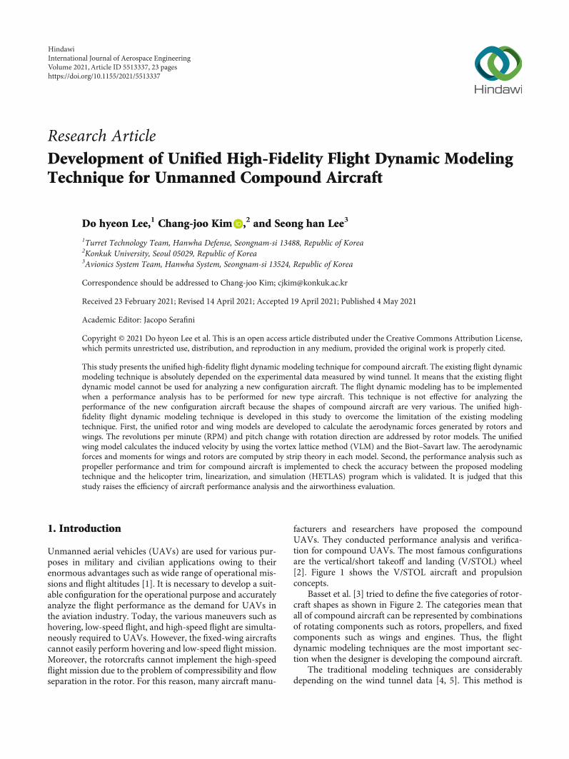
Basset et al. [3] tried to define the five categories of rotor-craft shapes as shown in Figure 2. The categories mean thatall of compound aircraft can be represented by combinationsof rotating components such as rotors, propellers, and fixedcomponents such as wings and engines. Thus, the flightdynamic modeling techniques are the most important sec-tion when the designer is developing the compound aircraft.

The traditional modeling techniques are considerablydepending on the wind tunnel data [4, 5]. This method is

HindawiInternational Journal of Aerospace EngineeringVolume 2021, Article ID 5513337, 23 pageshttps://doi.org/10.1155/2021/5513337

https://orcid.org/0000-0002-9493-7157

https://creativecommons.org/licenses/by/4.0/

https://doi.org/10.1155/2021/5513337

not efficiency because the experimental using wind tunnelhas to be perform for each aircraft. It is the limitation todevelop the aircraft system since the development cost andperiod are highly raised. Also, it is difficult to modify the flightdynamic model (FDM) according to the purpose of analysis orto add functions since the most FDM is distributed as com-mercial program [6]. The flight dynamic modeling techniqueshave been developed by several researchers to overcome thisdisadvantage. Kim et al. [7] studied the aerodynamic and iner-tial modeling of propeller. Cook et al. [4] and Etkins et al. [5]researched the flight dynamic principle. (1) Cook MV andEtkins used the traditional modeling techniques using windtunnel data. Leishman et al. [8] tried to develop the mathemat-ical helicopter aerodynamic model. Chaffin et al. [9] defined

the guide of the use for pressure disk rotor model. Taamallahet al. [10] studied the flight dynamic modeling for a small-scale helicopter UAV. Howlett et al. [11] developed the blackhawk engineering simulation program using mathematicalmodel. Pearson et al. [12] researched the aerodynamic charac-teristics of tapered wings. Talbot et al. [13] studied the mathe-matical model for single main rotor helicopter. Theresearchers in Ref [8–13] had tried to develop the mathemat-ical modeling technique for helicopter. However, (2) theseresearches can be used for certain aircraft. If the configurationsof aircraft are changed, the flight dynamicmodeling procedurehas to be newly started. This is the limitation for developingcompound aircraft because it is difficult to develop the flightdynamicmodel for each compound aircraft. It raises the devel-opment cost and period. So, most companies designing theaircraft system cannot try to develop the compound aircraft.(3) Therefore, the flight dynamic modeling technique has tobe developed to easily express the characteristics of all typecompound aircraft.

The contribution of this studied is the development ofunified flight dynamic modeling technique to overcome thedisadvantages of existing modeling techniques and to easilyimprove the fidelity of FDM while responding to changes inaircraft geometry. Especially, a unified rotor and wing modelsare developed to selectively calculate the aerodynamic forcesof the rotors with wings and to analyze the flight perfor-mance of any aircraft without modifying the mathematicalmodel. This technique can easily modify and add the rotoror wing models according to the analysis purpose.

The rest of this paper is organized as follows. Section 2introduces the unified aerodynamic component modelingtechnique, and Section 3 deals with the application to validatethe accuracy of proposed modeling method by comparingwith the HETLAS program. Section 4 is the conclusion of thisresearch.

V/STOL Aircra�and propulsionconcepts

Figure 1: V/STOL wheel [2].

Differentli�/propulsion Tilt blade

tip-path-plane

Rotor-> wings

Tilt-rot

or (T

R)

Tilt-wing

Tilt-body

Helicopter+ turbofan Helicopter

Coaxial

Notar

Tip jet

Inter-meshing

Tandem

Quad rotor

Multi rotorTail

sitter2TR, 4TRDucted TR

Swivel TR

Stoppablerotor

Variablerotor

radius

Rotodyne

Coaxial + turboprop

Bell 533 SA 365N Dauphin

Kamov KA 52

MD 900

MD XV-1

Kaman kmax

CH 47 chinook

Drone parrot

E-volo orvolocopter

Lockheed XVF-1Bell v22 osprey

Verticopterconcept

Rotoprop

Boeing X-50

Boeingdiscrotor

Eurocopter X3

Sikorsky X2

Figure 2: Five categories of rotorcrafts [3].

2 International Journal of Aerospace Engineering

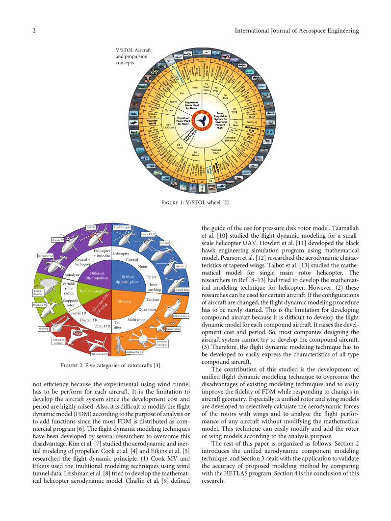
2. Unified Aerodynamic ComponentModeling Technique

This section describes the unified aerodynamic componentmodeling techniques for FDM. The traditional flightdynamic modeling techniques have used the wind tunnel testdata as mentioned in introduction. Its method allows to buildthe high-fidelity FDM. However, if the configurations of air-craft are changed, the FDM developed by the traditionalmodeling technique cannot be used for new aircraft. Thus,

this paper uses the unified component-based modeling tech-nique as shown in Figure 3. This technique builds each com-ponent model such as rotor, wing, fuselage, propeller, andduct after modeling the aerodynamic forces and moments.The FDM of all type configurations for compound aircraftcan be easily developed, and the flight dynamics analysis israpidly implemented. The main component model generat-ing aerodynamic forces and moments is the rotors and wings.Therefore, the aerodynamic modeling techniques of rotorsand wings are developed in this section.

Attitude kinematics

Position kinematics

u. + (wq–vr)+gsin𝜃 = X/mv. + (ur–wp)+gsin𝜙cos𝜃 = Y/mw. + (vp–uq)+gcos𝜙cos𝜃 = Z/m

Ixx p. – (Iyy–Izz)qr–Ixz( r

.+pq) = LIyy q

. + (Ixx–Izz)pr+Ixz(p2–r2) = MIzz r

. – (Ixx–Iyy)pq–Ixz(p.+qr) = N

Linear motion equations

Gravity forcesEuler attitude anglesQuaternionFinite rotation angles

Angular motion equations

Flight control system

Force summationX = XRotor+XWing+XFus+...

Y = YRotor+YWing+YFus+...

Z = ZRotor+ZWing+ZFus+...

L = LRotor+LWing+LFus+...

M = MRotor+MWing+MFus+...

N = NRotor+NWing+NFus+...

Moment summationPropeller/Ducted

Rotor

Wing/Control surf.

Fuselage

Power plant

Atmospheric conditionsturbulence modelwind shear modeletc.

Flight dynamic equationsExternal forces and moments

Figure 3: Component-based modeling technique.

Table 1: Classification of various rotors.

Rotor type Mounting position and orientation Available dynamics Control mechanism

Conventional mainrotor

-Top/center of fuselage-Vertical (reference) with small FWD

tilt angleFlap/lag/RPM Collective and 2 cyclic pitches

Conventional tailrotor

-Rear fuselage-±90 deg sideward tilt with small cant

angle

Flap/RPM (MRdependent)

Collective (pedal)

Teetering main rotor-Top/center of fuselage

-Vertical with small FWD tilt angleFlap Collective and 2 cyclic pitches

Teetering tail rotor-Rear fuselage

-±90 deg sideward tilt with small cantangle

Flap Collective (pedal)

ABC rotor (coaxial)-Top/center of fuselage

-Vertical with small FWD tilt angleNo

Collective and 2 cyclic pitches with differentialcollective

Propeller-Front (tractor) or rear (pusher) of

fuselage-±90 deg FWD tilt angle

No Collective or RPM

Ducted fan -Design dependent No Collective (thrust vectoring)

3International Journal of Aerospace Engineering

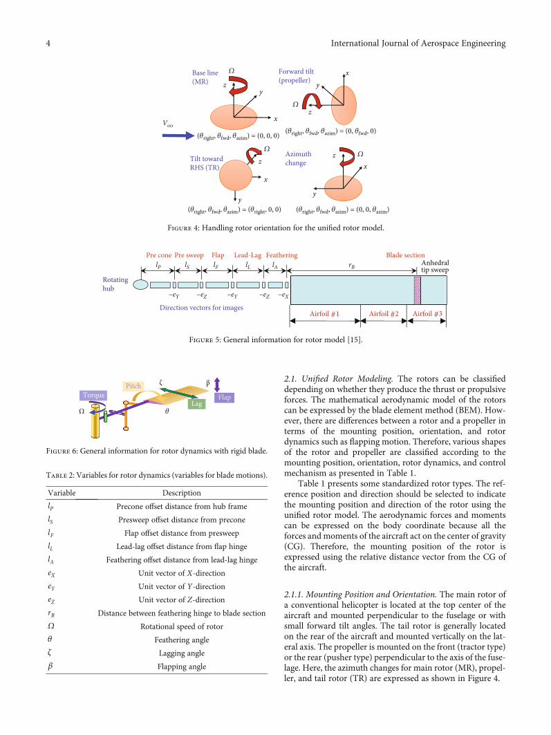
2.1. Unified Rotor Modeling. The rotors can be classifieddepending on whether they produce the thrust or propulsiveforces. The mathematical aerodynamic model of the rotorscan be expressed by the blade element method (BEM). How-ever, there are differences between a rotor and a propeller interms of the mounting position, orientation, and rotordynamics such as flapping motion. Therefore, various shapesof the rotor and propeller are classified according to themounting position, orientation, rotor dynamics, and controlmechanism as presented in Table 1.

Table 1 presents some standardized rotor types. The ref-erence position and direction should be selected to indicatethe mounting position and direction of the rotor using theunified rotor model. The aerodynamic forces and momentscan be expressed on the body coordinate because all theforces and moments of the aircraft act on the center of gravity(CG). Therefore, the mounting position of the rotor isexpressed using the relative distance vector from the CG ofthe aircraft.

2.1.1. Mounting Position and Orientation. The main rotor ofa conventional helicopter is located at the top center of theaircraft and mounted perpendicular to the fuselage or withsmall forward tilt angles. The tail rotor is generally locatedon the rear of the aircraft and mounted vertically on the lat-eral axis. The propeller is mounted on the front (tractor type)or the rear (pusher type) perpendicular to the axis of the fuse-lage. Here, the azimuth changes for main rotor (MR), propel-ler, and tail rotor (TR) are expressed as shown in Figure 4.

Base line(MR)

Forward tilt(propeller)

Tilt towardRHS (TR)

Azimuthchange

z

V∞

zz

z

y

yy

y

x

(𝜃right, 𝜃fwd, 𝜃azim) = (0, 0, 0)

(𝜃right, 𝜃fwd, 𝜃azim) = (0, 0, 𝜃azim)(𝜃right, 𝜃fwd, 𝜃azim) = (𝜃right, 0, 0)

(𝜃right, 𝜃fwd, 𝜃azim) = (0, 𝜃fwd, 0)

x

x

x𝛺

𝛺

𝛺𝛺

Figure 4: Handling rotor orientation for the unified rotor model.

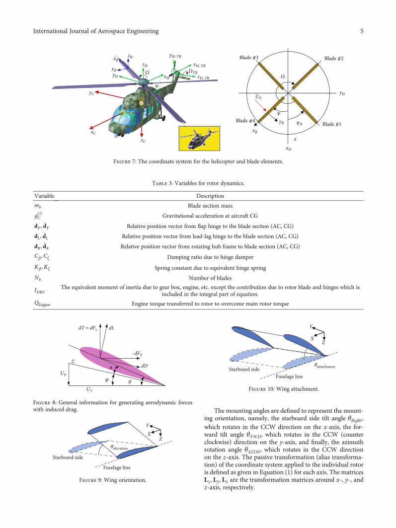
Pre cone Pre sweep Flap Lead-Lag Feathering Blade sectionrBlL lAlFlSlP

–eX–eZ–eY–eZ–eY

Rotatinghub

Direction vectors for imagesAirfoil #1 Airfoil #2

Anhedraltip sweep

Airfoil #3

Figure 5: General information for rotor model [15].

ζ β

TorqueLag

PitchFlap

𝜃Ω

Figure 6: General information for rotor dynamics with rigid blade.

Table 2: Variables for rotor dynamics (variables for blade motions).

Variable Description

lP Precone offset distance from hub frame

lS Presweep offset distance from precone

lF Flap offset distance from presweep

lL Lead-lag offset distance from flap hinge

lA Feathering offset distance from lead-lag hinge

eX Unit vector of X-direction

eY Unit vector of Y-direction

eZ Unit vector of Z-direction

rB Distance between feathering hinge to blade section

Ω Rotational speed of rotor

θ Feathering angle

ζ Lagging angle

β Flapping angle


The mounting angles are defined to represent the mount-ing orientation, namely, the starboard side tilt angle θRight ,which rotates in the CCW direction on the x-axis, the for-ward tilt angle θFWD, which rotates in the CCW (counterclockwise) direction on the y-axis, and finally, the azimuthrotation angle θAZIM , which rotates in the CCW directionon the z-axis. The passive transformation (alias transforma-tion) of the coordinate system applied to the individual rotoris defined as given in Equation (1) for each axis. The matricesL1, L2, L3 are the transformation matrices around x-, y-, andz-axis, respectively.

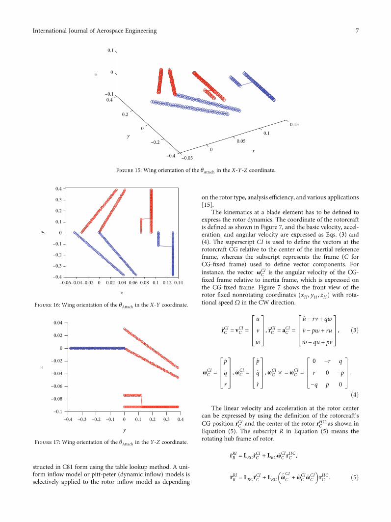
Blade #3 Blade #2

Blade #1Blade #4

xB

zC

zB

zH

xB

xC

UT

yB 𝜓R

𝜓

𝜓

xH

yH

yBxH

xH, TR

zH, TR

yH, TR

yHyC

x

ΩΩ ΩTR

Figure 7: The coordinate system for the helicopter and blade elements.

Table 3: Variables for rotor dynamics.


mb Blade section mass

gCIC Gravitational acceleration at aircraft CG

dF , �dF Relative position vector from flap hinge to the blade section (AC, CG)

dL, �dL Relative position vector from lead-lag hinge to the blade section (AC, CG)

dR, �dR Relative position vector from rotating hub frame to blade section (AC, CG)

C _β, C _ζ Damping ratio due to hinge damper

Kβ, Kζ Spring constant due to equivalent hinge spring

Nb Number of blades

IDRVThe equivalent moment of inertia due to gear box, engine, etc. except the contribution due to rotor blade and hinges which is

included in the integral part of equation.

QEngine Engine torque transferred to rotor to overcome main rotor torque

UP

UT

UdD

dLdT = dFz

–dFY

𝛼

𝜙 𝜃

Figure 8: General information for generating aerodynamic forceswith induced drag.

Starboard side

XY

Z

Fuselage line

𝜃elevation

Figure 9: Wing orientation.

Starboard side

X

Y

Z

Fuselage line

𝜃attachment

Figure 10: Wing attachment.


L1 xð Þ =1 0 0

0 cos x sin x

0 −sin x cos x

0BB@

1CCA,

L2 yð Þ =cos y 0 −sin y

0 1 0

sin y 0 cos y

0BB@

1CCA,

L3 zð Þ =cos z sin z 0

−sin z cos z 0

0 0 1

0BB@

1CCA:

ð1Þ

The reference for the mounting orientation is the orienta-tion of the conventional main rotor. The coordinate transfor-mation matrix from CG to the rotor hub LHC is defined asgiven in Equation (2).

LHC = L1 θRight� �

L2 π − θFWDð ÞL3 θAZIMð Þ: ð2Þ

Various rotor orientations can be expressed using thistransformation matrix. For instance, the conventional mainrotor is represented as ðθRight, θFWD, θAZIMÞ = ð0, 0, 0Þ,whereas the pusher propeller and tail rotor mounted on thestarboard side are expressed as ðθRight, θFWD, θAZIMÞ = ð−π/2, 0, 0Þ and ðθRight, θFWD, θAZIMÞ = ð0, π/2, 0Þ as shown inFigure 4, respectively.

2.1.2. Rotor Dynamics. The rotor and the propeller are sepa-rated based on the rotor dynamics. The rotor dynamics is notapplied when the propeller and ABC (advanced blade con-cept) rotor developed by Sikorsky are used [14]. Figures 5and 6 show the general information for rotor dynamics.The unified rotor dynamics can select the rotor dynamicsfor each rotor. Table 2 is the descriptions for variables ofrotor dynamics. The aerodynamic forces and moments ofthe blade elements are calculated using BEM. The aerody-namic coefficients corresponding to the angle of attack(AOA) and Mach number of the blade elements are esti-mated from the nonlinear aerodynamic coefficient table con-

–0.06 –0.04 –0.02 0 0.02 0.04 0.06 0.08 0.1 0.12 0.14–0.4

–0.3

–0.2

–0.1

0

0.1

0.2

0.3

x

y

Figure 12: Wing orientation of the θElev in the X-Y coordinate.

–0.4 –0.3 –0.2 –0.1 0 0.1 0.2 0.30

0.05

0.1

0.15

0.2

0.25

0.3

0.35

y

z

Figure 13: Wing orientation of the θElev in the Y-Z coordinate.

–0.050

0.050.1

0.15

–0.4–0.2

00.2

0.40

0.1

0.2

0.3

0.4

xy

z

Figure 11: Wing orientation of the θElev in the X-Y-Z coordinate.

–0.06 –0.04 –0.02 0 0.02 0.04 0.06 0.08 0.1 0.12 0.140

0.05

0.1

0.15

0.2

0.25

0.3

0.35

y

z

Figure 14: Wing orientation of the θElev in the X-Z coordinate.


structed in C81 form using the table lookup method. A uni-form inflow model or pitt-peter (dynamic inflow) models isselectively applied to the rotor inflow model as depending

on the rotor type, analysis efficiency, and various applications[15].

The kinematics at a blade element has to be defined toexpress the rotor dynamics. The coordinate of the rotorcraftis defined as shown in Figure 7, and the basic velocity, accel-eration, and angular velocity are expressed as Eqs. (3) and(4). The superscript CI is used to define the vectors at therotorcraft CG relative to the center of the inertial referenceframe, whereas the subscript represents the frame (C forCG-fixed frame) used to define vector components. Forinstance, the vector ωCI

C is the angular velocity of the CG-fixed frame relative to inertia frame, which is expressed onthe CG-fixed frame. Figure 7 shows the front view of therotor fixed nonrotating coordinates ðxH , yH , zHÞ with rota-tional speed Ω in the CW direction.

_rCIC = vCIC =

u

v

w

2664

3775,€rCIC = aCIC =

_u − rv + qw

_v − pw + ru

_w − qu + pv

2664

3775, ð3Þ

ωCIC =

p

q

r

2664

3775, _ωCI

C =

_p

_q

_r

2664

3775, ωCI

C × = ~ωCIC =

0 −r q

r 0 −p

−q p 0

2664

3775:

ð4ÞThe linear velocity and acceleration at the rotor center

can be expressed by using the definition of the rotorcraft’sCG position rCIC and the center of the rotor rHC

C as shown inEquation (5). The subscript R in Equation (5) means therotating hub frame of rotor.

_rRIR = LRC _rCIC + LRC~ωCIC rHC

C ,

€rRIR = LRC€rCIC + LRC _~ωCIC + ~ωCI

C ~ωCIC

� �rHCC : ð5Þ

–0.050

0.050.1

0.15

–0.4

–0.2

0

0.2

0.4–0.1

0

0.1

x

y

z

Figure 15: Wing orientation of the θAttach in the X-Y-Z coordinate.

–0.06–0.04–0.02 0 0.02 0.04 0.06 0.08 0.1 0.12 0.14–0.4

–0.3

–0.2

–0.1

0

0.1

0.2

0.3

0.4

x

y

Figure 16: Wing orientation of the θAttach in the X-Y coordinate.

–0.4 –0.3 –0.2 –0.1 0 0.1 0.2 0.3 0.4–0.1

–0.08

–0.06

–0.04

–0.02

0

0.02

0.04

y

z

Figure 17: Wing orientation of the θAttach in the Y-Z coordinate.


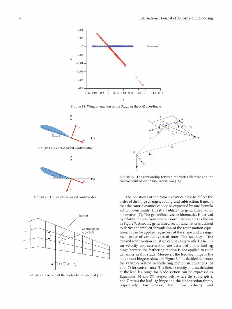
The equations of the rotor dynamics have to reflect theorder of the hinge changes, adding, and subtraction. It meansthat the rotor dynamics cannot be expressed by one formulawithout constraints. This study utilizes the generalized vectorkinematics [7]. The generalized vector kinematics is derivedby relative motion from several coordinate systems as shownin Figure 7. Also, the generalized vector kinematics is utilizedto derive the implicit formulation of the rotor motion equa-tions. It can be applied regardless of the shape and arrange-ment order of various types of rotor. The accuracy of thederived rotor motion equation can be easily verified. The lin-ear velocity and acceleration are described at the lead-laghinge because the feathering motion is not applied to rotordynamics in this study. Moreover, the lead-lag hinge is theouter most hinge as shown in Figure 5. It is decided to denotethe variables related in feathering motion in Equations (6)and (7) for convenience. The linear velocity and accelerationat the lead-lag hinge for blade section can be expressed asEquations (6) and (7), respectively, where the subscripts Land T mean the lead-lag hinge and the blade section frame,respectively. Furthermore, the linear velocity and

–0.06 –0.04 –0.2 0 0.02 0.04 0.06 0.08 0.1 0.140.12–0.1

–0.08

–0.06

–0.04

–0.02

0

0.02

0.04

y

z

Figure 18: Wing orientation of the θAttach in the X-Z coordinate.

X

Z

un

uc

𝜃twist

Figure 19: General airfoil configuration.

X

Z

un

uc

𝜃twist

Figure 20: Upside-down airfoil configuration.

Panel n

Control pointrCP = 3c/4

Γn

c

Figure 21: Concept of the vortex lattice method [16].

FC

P

rP

rv

dll

rA

A

B

rB

h𝜃A

𝜃Bu

xc

yc

zc

𝜃

Figure 22: The relationship between the vortex filament and thecontrol point based on biot-sarvart law [16].


acceleration are defined on CG and AC of the blade section toreflect the rotor dynamics and to calculate the aerodynamicforces, respectively.

_rTIL = LLR _rRIR + LLR~ωRIR LRL

� lPLLR + lSLLP + lFLLS + lLLLF + lAð ÞeXf g� − _βLLSE2LSL lLLLF + lAð ÞeX − σ _ζLLFE3LFLlAeXh

+LLR~ωRI

R LRL − _βLLSE2LSL

−σ _ζLLFE3LFL + σ _θE1

8<:

9=;

� rBLLAeX − σySLLTeY − zALLTeZð Þ�,

ð6Þ

€rTIL = LLR€rRIR + LLR _~ωRIR + ~ωRI

R ~ωRIR

� �LRL lPLLR + lSLLP + lFLLSð ÞeX

+ LLR _~ωRIR + ~ωRI

R ~ωRIR

� �LRL + LLS −€βI + _β

2E2

� �E2LSL

n

+ LLF −σ€ζI + _ζ2E3

� �LFLE3 + 2σ _β _ζLLSE2LSLE3

+ LLR~ωRIR LRL −2 _βLLSE2LSL − 2σ _ζE3

� �orBeX :

ð7ÞThe velocity _rTIL is composed by three parts such as linear

velocity, angular velocity from lead-lag hinge, and effect ofthe angular rate from lead-lag hinge to the blade section.Although the acceleration as Equation (7) can be derived byusing similar way to define Equation (6), the only differencebetween Equation (7) and Equation (6) is that Equation (6)considers the sweep length yS and an hedral length zA. Thevariable σ denotes the rotating direction which is CW rota-tion (σ = −1) and CCW rotation (σ = 1).

The flap, lead-lag, and RPM dynamics associated withrotor motion are defined as Equations (8)–(10), respectively.Each dynamics can be selectively used by rotor type. If therotor type is defined as the propeller, the rotor motion doesnot apply as noticed in Table 1, whereas if the general rotoris selected, the rotor motion is used. Moreover, the relativeangles such as flapping angles are computed with each rotormotion. The flapping motion occurs of the y-axis associatedwith rotating rotor hub frame because of the flap hinge.The unit vector of y-axis and z-axis on rotor hub frame isdefined as eY and eZ , respectively. The lead-lag and RPM

dynamics move on the z-axis as the same principle of flap-ping motion. The flapping motion and RPM dynamics areneeded to consider rotating direction additionally. The

FBF, A, MBF, A FW, A, MW, ArWG

rVS rHS

VS: strip

HS: strip

MG: strip

r

Figure 23: Concept of strip theory [16].

𝛼 = tan–1 (|Vn/Vc|), where Vc > 0, Vn > 0

un

uc

Vac

Vc Vn

Figure 24: AOA with Vc > 0, Vn > 0.

𝛼 = –tan–1 (|Vn/Vc|), where Vc > 0, Vn < 0

un

uc

Vac Vc

Vn

Figure 25: AOA with Vc > 0, Vn < 0.

𝛼 = 𝜋/2+tan–1 (|Vn/Vc|), where Vc < 0, Vn > 0

un

uc

Vac

Vc

Vn

Figure 26: AOA with Vc < 0, Vn > 0.

𝛼 = –𝜋/2+tan–1 (|Vn/Vc|), where Vc < 0, Vn < 0

un

ucVac

Vc Vn

Figure 27: AOA with Vc < 0, Vn < 0.


RPM dynamics does not consider the damping ratio andspring constant because the rotor shaft linked directly tothe gear box and engine. So, the inertia forces in Equation(10) are divided as two forces generated by acceleration atthe blade section and shaft IDRV _Ω, respectively. The variableswhich use in the following equations are listed in Table 3.

ðmB

�dF × LFL€rTIL − LFCgCIC� �

⋅ eYdrB − C _β_β − Kββ

=ðLFLdMAero

Sec + dF × LFLdFAeroSec� �

⋅ eY ,ð8Þ

σðmB

�dL × €rTIL − LLCgCIC� �

⋅ eZdrB − C _ζ_ζ − Kζζ

= σðdMAero

Sec + dL × dFAeroSec� �

⋅ eZ ,ð9Þ

〠Nb

J=1σ

ðmB

�dR × LRL€rTIL − LRCgCIC� �

⋅ eZdrB� �

+ IDRV _Ω

= 〠Nb

J=1σ

ðLRLdMAero

Sec + dR × LRLdFAeroSec� �

⋅ eZ� �

+QEngine:

ð10ÞThe aerodynamic forces dFAeroSec and moments dMAero

Sec forthe unit section on the blade have to be calculated to computethe flap, lead-lag, and RPM dynamics. Figure 8 shows thegeneral information for generating aerodynamic forces withinduced drag at the blade section. The aerodynamic forcesgenerated by blade section can be defined as Equation (11).

dFAeroL =

dR

σ −dL sin ϕ − dD cos ϕð ÞdL cos ϕ − dD sin ϕ

0BB@

1CCA, dMAero

L =

σdM

0

0

0BB@

1CCA,

ð11Þ

ϕ = tan−1UP

UT

, α = θ − ϕ = θ − tan−1

UP

UT

, ð12Þ

where dR, dL, dD, and dM are the spanwise axial forces,lift, drag, and moment on the unit section for blade,respec-tively, to calculate the aerodynamic forces. These four vari-ables are expressed as Equation (13).

dL =12CLρ U2

T +U2P

� �cdrB, dD =

12CDρ U2

T +U2P

� �cdrB,

dR =12CRρ U2

T +U2P

� �cdrB, dM =

12CDρ U2

T +U2P

� �c2drB:

ð13Þ

Here, c is the distance of the camber for blade. CL, CD,and CR are the aerodynamic coefficients for lift, drag, andspanwise axial force, respectively. The coefficients are esti-mated using C81 tables by table-lookup technique. Espe-cially, the table-lookup technique can change the

coefficients when the blade has the conversion section. Thevelocity component to generate the aerodynamic forces andmoment can be defined as follow.

UR

UT

UP

2664

3775 =

VLX

VLY

VLZ

2664

3775 = vTIL − vturL − vindL = vaeroL : ð14Þ

vTIL , vturL , and vindL mentioned in Equation (14) are _rTIL , tur-bulence, and induced inflow, respectively.

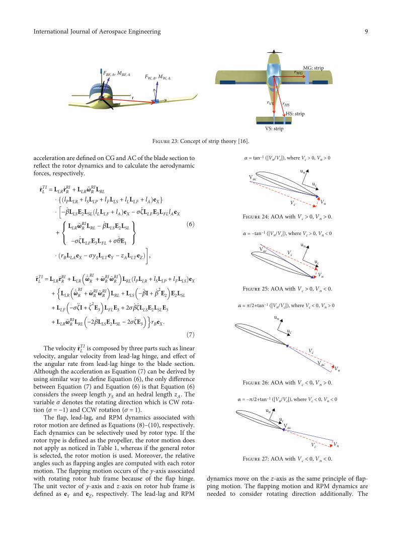
2.2. Unified Wing Modeling: Geometry. The wings have vari-ous shapes and are usually attached to the center of the fuse-lage for aircraft. The wings are classified by mounted positionand purpose of control surface to construct a unified wingmodel that can reflect all characteristics of the wings.

A typical fixed wing aircraft is equipped with five wingssuch as the left and right main wings, the left and right hor-izontal stabilizers, and the vertical stabilizer. However, acompound rotorcraft can be made with wings at variousangles and positions. This is the reason why the unified wingmodeling technique has to be developed. The unified wing

0 5 10 15 20 25 300

0.2

0.4

0.6

0.8

1

1.2

1.4

clsu

rface

control surface deflection δsurface

�eory by chester�eory by torenbeek

�eory by datcomReference

Figure 28: Comparison results for lift coefficient computed byseveral theories and wind tunnel data [21].

Table 4: The specification associated with wing model.


Airfoil NACA23012

t/c 0.12

csurface 0:2cairfoil

Clα0.1080 (/deg)6.1879 (/rad)

AOA 0 (deg)

Reynolds number 8:0 × 106

Deflection of control surface 0:0 < δsurface < 30:0 (deg)


model is capable of reflecting various wing shapes and posi-tions. The mounting angle is based on the starboard sidewing, and the wing coordinate is the same as the body coor-dinate of the aircraft. Three different angles are defined torepresent the wing mounting angles such as elevation angleθElev , attachment angle θAttach, and rotation angle θRot. θElevrotates in the CW direction of the x-axis, and θAttach rotatesin the CCW direction of the y-axis. Finally, θRot rotates inthe CW direction of the z-axis. The x -, y-, and z-axis coordi-nate rotation matrices (active transformation matrix) definedin Equation (1) are applied for the rotation of the wing. Thus,the wing coordinate rotation matrix LWING using Equation(1) is defined as given in Equation (15).

LWING = L1 θElevð ÞL2 θAttachð ÞL3 θRotð Þ: ð15Þ

The unified wing model can handle the angle of elevation,attachment, and rotation angle for wing. The elevation angleθElev and the attachment angle θAttach for wing can be definedas shown in Figures 9 and 10. The fuselage line and the star-board side of the wing are the standard line to define eachangle. Figures 11–14 show the results of wing orientationfor elevation angle θElev. The blue color expresses the portwing, and the red color means the starboard wing inFigures 11–14. Figure 11 shows the wing orientations onthe X-Y-Z coordinate when the elevation angle for starboardside wing and port side wing are defined as 45 (deg) and 0(deg), respectively. Moreover, the attachment angles aresame as 0 (deg) for port side and starboard side.Figures 12–14 are expressing the wing orientation resultson the X-Y , Y-Z, and X-Z coordinate, respectively. This isthe very useful function to make the geometry for variouscompound aircraft.

Figures 15–18 show the wing geometry when the attach-ment angles of starboard side and port side wing are definedas 45 (deg) and 0 (deg). The difference between the starboardside and the port side is expressed on the X-Y-Z coordinatein Figure 15. The attachment angles for each wing can be

HETLASSubsystems

Actuatorsubsystem

Signalgeneratorsubsystem

Sensorsubsystem

FCSsubsystem

Helicoptertrim

Linearization

Flightsimulation

Pilotsubsystem

6–DoF

Helicopter math model

Main rotorMain rotor

inflow

Tail rotorTail rotor

inflow

Fuselage

Empennage

Torque

AerodynamicDBs

Control lawdesign

Time domainanalysis

Control lawauto-code

Figure 29: The structure of the HETLAS program [18].

Table 5: The configuration data for reference helicopter [19].

Configurations Data

Length 19.0 (m)

Rotor diameter 15.8 (m)

Height 4.5 (m)

Maximum takeoff weight 8,709 (kg)

Engine 1, 855 × 2 (SHP)

Maximum cruise speed 279 (km/h)

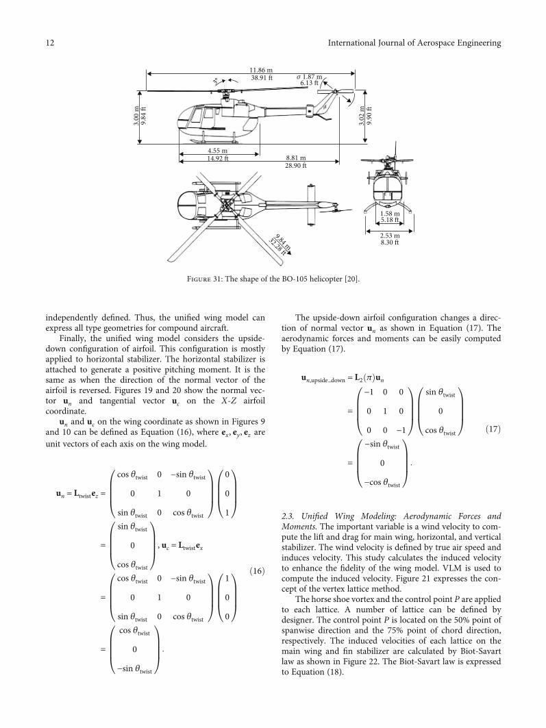
Figure 30: The shape of the reference helicopter [19].

Table 6: The configuration data for the BO-105 helicopter [20].

Configurations Data

Length 11.8 (m)

Rotor diameter 9.8 (m)

Height 3.0 (m)

Maximum takeoff weight 2,500 (kg)

Engine 420 × 2 (SHP)

Maximum cruise speed 268 (km/h)


independently defined. Thus, the unified wing model canexpress all type geometries for compound aircraft.

Finally, the unified wing model considers the upside-down configuration of airfoil. This configuration is mostlyapplied to horizontal stabilizer. The horizontal stabilizer isattached to generate a positive pitching moment. It is thesame as when the direction of the normal vector of theairfoil is reversed. Figures 19 and 20 show the normal vec-tor un and tangential vector uc on the X-Z airfoilcoordinate.

un and uc on the wing coordinate as shown in Figures 9and 10 can be defined as Equation (16), where ex, ey, ez areunit vectors of each axis on the wing model.

un = Ltwistez =

cos θtwist 0 −sin θtwist

0 1 0

sin θtwist 0 cos θtwist

0BBB@

1CCCA

0

0

1

0BBB@

1CCCA

=

sin θtwist

0

cos θtwist

0BBB@

1CCCA, uc = Ltwistex

=

cos θtwist 0 −sin θtwist

0 1 0

sin θtwist 0 cos θtwist

0BBB@

1CCCA

1

0

0

0BBB@

1CCCA

=

cos θtwist

0

−sin θtwist

0BBB@

1CCCA:

ð16Þ

The upside-down airfoil configuration changes a direc-tion of normal vector un as shown in Equation (17). Theaerodynamic forces and moments can be easily computedby Equation (17).

un,upside down = L2 πð Þun

=

−1 0 0

0 1 0

0 0 −1

0BBB@

1CCCA

sin θtwist

0

cos θtwist

0BBB@

1CCCA

=

−sin θtwist

0

−cos θtwist

0BBB@

1CCCA:

ð17Þ

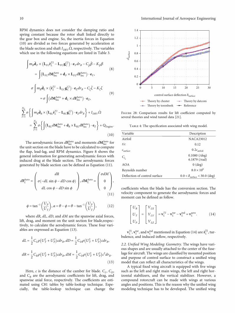
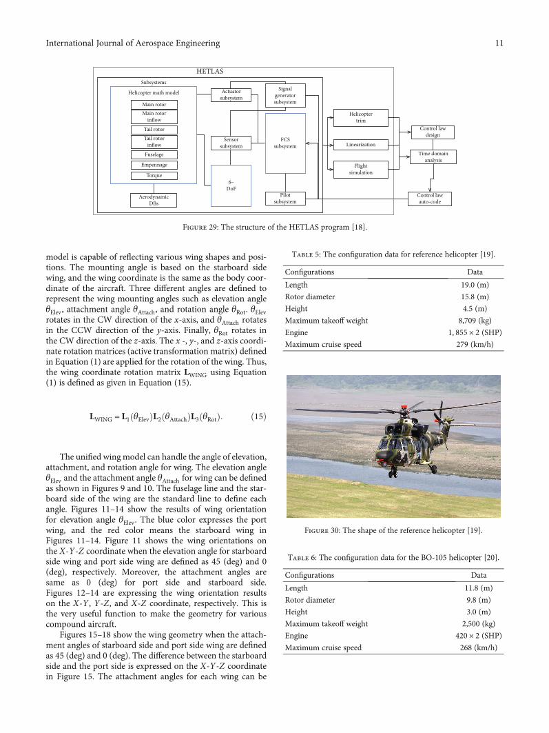
2.3. Unified Wing Modeling: Aerodynamic Forces andMoments. The important variable is a wind velocity to com-pute the lift and drag for main wing, horizontal, and verticalstabilizer. The wind velocity is defined by true air speed andinduces velocity. This study calculates the induced velocityto enhance the fidelity of the wing model. VLM is used tocompute the induced velocity. Figure 21 expresses the con-cept of the vertex lattice method.

The horse shoe vortex and the control point P are appliedto each lattice. A number of lattice can be defined bydesigner. The control point P is located on the 50% point ofspanwise direction and the 75% point of chord direction,respectively. The induced velocities of each lattice on themain wing and fin stabilizer are calculated by Biot-Savartlaw as shown in Figure 22. The Biot-Savart law is expressedto Equation (18).

11.86 m38.91 � 𝜎 1.87 m

6.13 �

3.02

m9.

90 �

4.55 m14.92 � 8.81 m

28.90 �

9.84 m32.28 �

1.58 m5.18 �

2.53 m8.30 �

3.00

m9.

84 �

3°

Figure 31: The shape of the BO-105 helicopter [20].


dVind rPð Þ = Γ

4πdl × rrk k3 =

Γ

4πdl × rP − rvð Þ

rP − rvk k3

= Γch2

4πffiffiffiffiffiffiffiffiffiffiffiffiffir2c + h2

q dl × rP − rvð ÞrP − rvk k3 :

ð18Þ

FC means an origin point of the body coordinate. rP andrv are a distance vector from the origin point of the bodycoordinate to control point of each lattice and to unit vortexfilament dl, respectively. rc is a core radius for vortex fila-ment, and h is a perpendicular distance from vertex filamentto control point P. If the number of lattice is increased, thenumber of control point is expended. The lift of each latticecan be computed by Equation (19).

L = ρVΓc, ð19Þ

where ρ and V are the density of air and the true airspeed, respectively. Γc is the vortex strength. Kutta-

Joukowski theory as shown in Equation (20) is used to com-pute Γc.

Γc =12CLVs: ð20Þ

CL and s are the lift coefficient and the area of unit sec-tion. Finally, the velocity V has to be computed, and it is akVack. Vac is a velocity vector that the Y-component is zero.The velocity vector is calculated after computing vk. vk is avelocity vector including the Y-component on each lattice.The subscript of vk is a number of lattice in the main wingand fin stabilizer. vk is defined as Equation (21).

vk = vCIC + ~ωCIC rPCC + vind,k, ð21Þ

where vCIC is a true air speed vector associated with CG,and ωCI

C is a angular velocity vector of aircraft. rPCC is a dis-tance vector between the CG of aircraft and the control point

0 50 1004

4.5

5

5.5

6

Colle

ctiv

e (de

g)

No dynamicsFlap dynamicsFlap + Lag dynamics

6

8

10

12

14

16

Indu

ced

velo

city

(m/s

)

1

1.1

1.2

1.3

1.4

1.5

1.6 x 105

�ru

st (N

)

0 50 1005

6

7

8

9

10 x 104

Torq

ue (N

·m)

0

2

4

6

8

Velocity (kn)

Flap

ping

angl

e (de

g)

–2

–1.5

–1

–0.5

0Le

ad la

g A

ngle

(deg

)

0 50 100

Velocity (kn)

0 50 100

0 50 100

0 50 100

Figure 32: Results of rotor performance analysis.


P of each lattice. vind,k is a induced velocity vector of each lat-tice.

Vac = vk − vk ⋅ ey� �

ey =Vc +Vn = Vcuc +Vnun: ð22Þ

ey is defined as shown in Equation (23).

ey = − uc × unð Þ: ð23Þ

The calculated aerodynamic forces and moments foreach lattice have to be expressed on the body coordinate. This

study use the strip theory to incorporate the aerodynamicforces and moments on the origin point of the body coordi-nate. The CG is the same with the origin point of the bodycoordinate. Figure 23 shows the concept of strip theory.

Thus, the computed aerodynamic forces and moments ofeach lattice can be expressed on CG as shown in Equation(24). Here, α and β are the AOA and the sideslip angle(SSA), respectively.

FPCC = LCPFPCP =

−D cos α cos β − Y cos α sin β + L sin α

−D sin β + Y cos β

−D sin α cos β − Y sin α sin β − L cos α

2664

3775,

MPCC = LCPMPC

P =

Mx cos α cos β −My cos α sin β −Mz sin α

Mx sin β +My cos β

Mx sin α cos β −My sin α sin β +Mz cos α

2664

3775:

ð24Þ

0 0.05 0.1 0.15 0.2 0.250

0.2

0.4

0.6

0.8

1

Effici

ency

: Col –8 deg: Col –4 deg: Col 0 deg

: Col 4 deg: Col 8 deg

0

200

400

600

800

1000

P req

(hp)

0

2000

4000

6000

8000

Advance ratio

�ru

st (N

)

0 0.05 0.1 0.15 0.2 0.25

0 0.05 0.1 0.15 0.2 0.25

Figure 33: Results of propeller performance analysis.

1.364 S/b0.682 S/b

c/4line

Figure 34: Configuration of tapered wing without control surface.


The aerodynamic forces and moments of main wing andfin stabilizers can be calculated by applying Equation (24) toall of lattice as shown in Equation (25).

〠FPCC = 〠n

j=1LCPFPCPj

,

〠MPCC = 〠

n

j=1LCPMPC

Pj+ rPCCj

× LCPFPCPj

� �,

ð25Þ

where the subscript j of the P is order of lattice for mainwing and fin stabilizer. So, jth control point P is described asPj.

2.4. Unified Wing Modeling: Aerodynamic Coefficients. TheAOA is calculated by 4 cases by using the absolute values ofvelocities. Each case is described as shown in Figures 24–27.

The influence of the wing lift coefficient on the controlsurface deflection is expressed as given in Equation (26).The control surface is considered as a plain flap. Here,Cl,surface and δsurface are the lift coefficient associated with con-trol surface and control surface deflection angle, respectively.

Cl = Cl,0 + Clαα + Cl,surfaceδsurface:: ð26Þ

The main coefficient in Equation (26) is a Cl,surfacebecause other coefficients such as Cl,0 and Clα

are the con-stant or the functions associated with AOA, SSA, and Machnumber. Thus, the calculation accuracy of Cl,surface is the mostimportant for the wing model. Several tools such as chester,

torenbeek, and DATCOM have suggested the theory to cal-culate the coefficient Cl,surface. A comparison of variousempirical formulas calculating Cl,surface indicates that the the-ory proposed in DATCOM is the most accurate as shown inFigure 28 [17]. The reference data in Figure 28 is the windtunnel test data for NACA23012 airfoil. The specification ofNACA23012 airfoil is described in Table 4. This study selectsthe theory proposed in DATCOM to compute Cl,surface.

3. Application

This section tries to validate the FDM built by the unifiedrotor and wing model. The single rotor helicopter and com-pound helicopter using coaxial rotor are used for checkingfidelity of FDM. The helicopter models are used to the BO-105 helicopter and the reference rotorcraft which is built byHETLAS. A reference rotorcraft is a Surion helicopter.HETLAS is a program for implementing trim, linearization,and simulation of the helicopter. Especially, this programhad been validated by the Surion helicopter. Moreover, ithas been already used to develop the FBW (fly-by-wire) sys-tem for Surion helicopter. Figure 29 shows the structure ofthe HETLAS program. The detail information of HETLASis described in Ref. [15, 18].

The configuration data for reference helicopter aredescribed as Table 5, and Figure 30 shows the shape of refer-ence helicopter.

The configuration data and shape for the BO-105 heli-copter are described as Table 6 and Figure 31, respectively.

The validation of proposed FDM would be conducted bycomparing with analysis results computed from the HETLASprogram. Trim analysis of the reference helicopter and simu-lation for the BO-105 rotorcraft in the time domain are usedas the validation method for proposed FDM.

The trim analysis of the reference helicopter would beimplemented by the HETLAS program and proposed FDM,where the validation of fidelity for proposed FDM is con-ducted by checking the difference of trim results betweenthe HETLAS program and proposed FDM since the almost

: Wing theory: Reference data

–15 –10 –5 0 5 10 15 20–1.5

–1

–0.5

0

0.5

1

1.5

AOA (deg)

Li�

coeffi

cien

t, C L

Tapered wing of AR 6, NACA 23012 airfoil

–15 –10 –5 0 5 10 15 20 250

0.05

0.1

0.15

0.2

0.25

AOA (deg)

Dra

g co

effici

ent,

C D


Figure 35: Comparison of the lift and drag coefficient.

0. 5b 1.364 S/b0.682 S/b

c/4line

Figure 36: Configuration of tapered wing with control surface.


analysis and experimental data of reference helicopter are theconfidential data. The simulation of the BO-105 helicopterwould be performed by proposed FDM because the flight testdata of the BO-105 helicopter has been opened. Especially,the AC-120 (advisory circular 120) criteria are applied tothe simulation process to compare thoroughly.

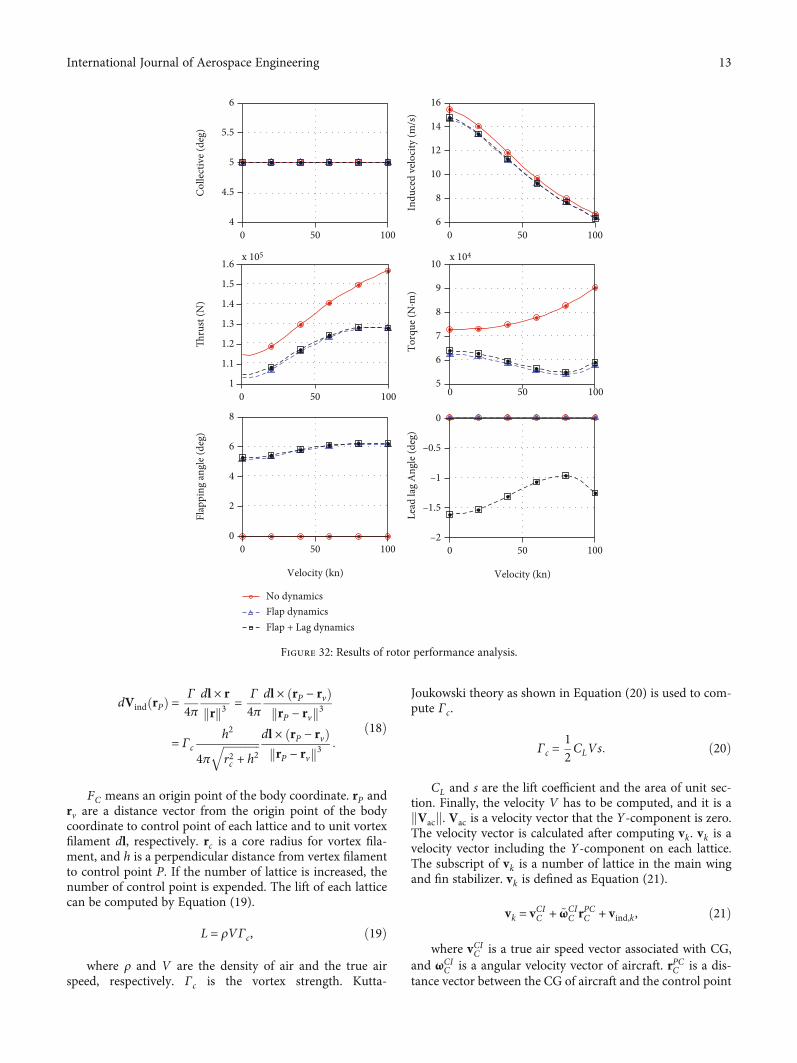
3.1. Unified Rotor Model. This study shows that the rotormodel employing the unified technique can be used to ana-lyze various types of rotor dynamics. This study uses therotor model validated by the HETLAS program. Figures 32and 33 show the aerodynamic analysis results of the rotorand propeller using the unified rotor model.

The rotor of a typical helicopter is used for analyzingrotor performance as shown in Figure 32. The main rotor isused for analysis, and the collective inputs are defined as 5degrees under the normal working states with increased for-ward speed. All results are compared with no rotor dynamics,flap dynamics, and flap and lag dynamics. The induced veloc-ity has been decreased when the flight speed is raised. Theinduced velocity is inversely proportional to forward speedas vi = T/2ρAV∞ as understanding the momentum theory.The induced velocity is significantly decreased as forwardspeed increased as shown in Figures 32 and 33. Althoughthe induced velocity is similar responses, the torques repre-sent different behaviors. Torque with no dynamics is steadilyincreased, but the others have maintained those values. Thisis because the AOA of the blade section affects the drag forceof the blade section. The drag coefficient at the blade sectionis reduced with a small effective AOA due to the increasingforward speed UT and the decreasing induced velocity UPas shown in Figure 8. This is the main reason to maintainthe torque level. Furthermore, the flapping angles whichcan be considered as damping effect make the significant biasamong all speed regions. The lag dynamics with negativelead-lag angles show less effect to torques increasing as aslightly bigger effective AOA with changing UT .

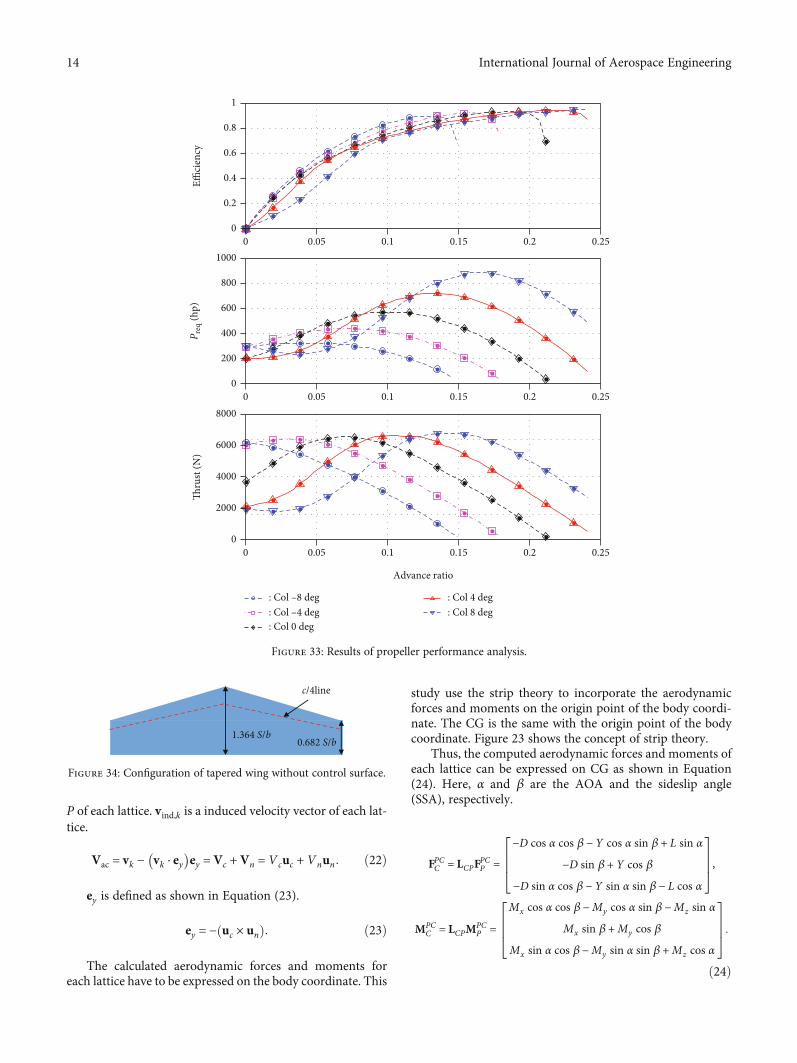
The tractor-type propeller is used for analyzing propellerperformance as shown in Figure 33 [7]. It shows the result ofthe analysis associated with advanced ratio and collectivechange. The thrusts and the required powers of the propellerhave been increased when the advance ratio and collectiveinput are raised, because the increments of flow velocity forpropeller make the effective AOA of the blade section fallsin the stall region. It means that the maximum thrust levelis almost constant when the effective AOA is in the stallregion. Furthermore, the propeller efficiency can be reachedto maximum point.

Figures 32 and 33 have showed that the rotor dynamicscan be selectively applied. Therefore, it is judged that the uni-fied rotor model is highly effective to calculate the aerody-namic forces of various types of rotor or propeller.

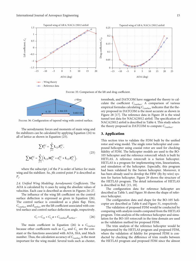
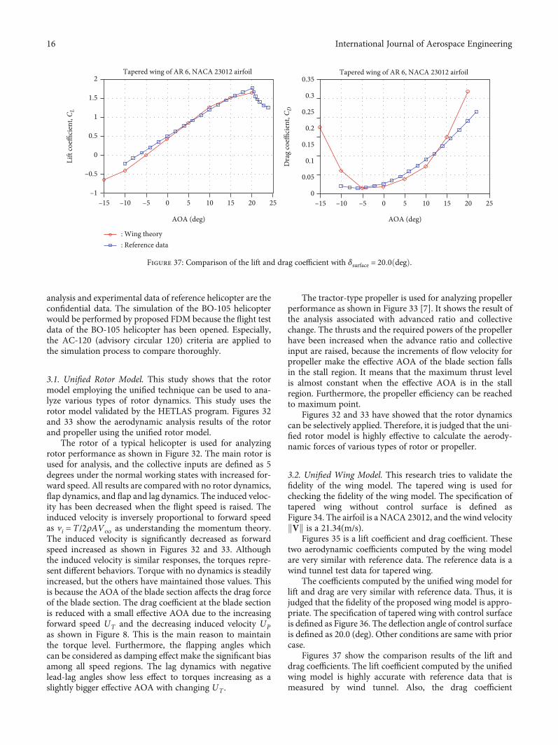
3.2. Unified Wing Model. This research tries to validate thefidelity of the wing model. The tapered wing is used forchecking the fidelity of the wing model. The specification oftapered wing without control surface is defined asFigure 34. The airfoil is a NACA 23012, and the wind velocitykVk is a 21.34(m/s).

Figures 35 is a lift coefficient and drag coefficient. Thesetwo aerodynamic coefficients computed by the wing modelare very similar with reference data. The reference data is awind tunnel test data for tapered wing.

The coefficients computed by the unified wing model forlift and drag are very similar with reference data. Thus, it isjudged that the fidelity of the proposed wing model is appro-priate. The specification of tapered wing with control surfaceis defined as Figure 36. The deflection angle of control surfaceis defined as 20.0 (deg). Other conditions are same with priorcase.

Figures 37 show the comparison results of the lift anddrag coefficients. The lift coefficient computed by the unifiedwing model is highly accurate with reference data that ismeasured by wind tunnel. Also, the drag coefficient

: Wing theory: Reference data

–15 –10 –5 0 5 10 15 25–1

–0.5

0

0.5

1

1.5

2

AOA (deg)

Li�

coeffi

cien

t, C L


20 –15 –10 –5 0 5 10 15 20 250

0.1

0.05

0.15

0.2

0.25

0.35

0.3

AOA (deg)

Dra

g co

effici

ent,

C D


Figure 37: Comparison of the lift and drag coefficient with δsurface = 20:0ðdegÞ.


calculated by the unified wing model is accurately computed.It is judged that the proposed wing modeling technique ishighly accurate.

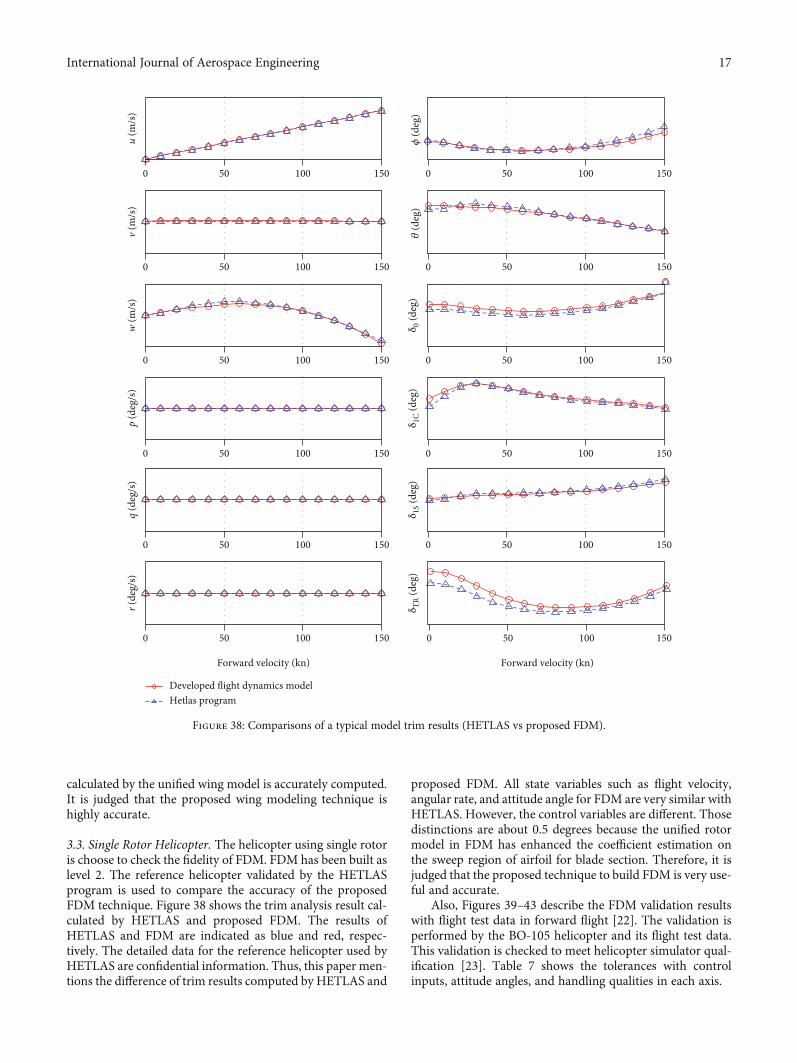
3.3. Single Rotor Helicopter. The helicopter using single rotoris choose to check the fidelity of FDM. FDM has been built aslevel 2. The reference helicopter validated by the HETLASprogram is used to compare the accuracy of the proposedFDM technique. Figure 38 shows the trim analysis result cal-culated by HETLAS and proposed FDM. The results ofHETLAS and FDM are indicated as blue and red, respec-tively. The detailed data for the reference helicopter used byHETLAS are confidential information. Thus, this paper men-tions the difference of trim results computed by HETLAS and

proposed FDM. All state variables such as flight velocity,angular rate, and attitude angle for FDM are very similar withHETLAS. However, the control variables are different. Thosedistinctions are about 0.5 degrees because the unified rotormodel in FDM has enhanced the coefficient estimation onthe sweep region of airfoil for blade section. Therefore, it isjudged that the proposed technique to build FDM is very use-ful and accurate.

Also, Figures 39–43 describe the FDM validation resultswith flight test data in forward flight [22]. The validation isperformed by the BO-105 helicopter and its flight test data.This validation is checked to meet helicopter simulator qual-ification [23]. Table 7 shows the tolerances with controlinputs, attitude angles, and handling qualities in each axis.

Hetlas program

0 50 100 150

u (m

/s)

v (m

/s)

0 50 100 150

w (m

/s)

0 50 100 150

p (d

eg/s

)

0 50 100 150

q (d

eg/s

)

0 50 100 150

Forward velocity (kn)

r (de

g/s)

0 50 100 150

𝜙 (d

eg)

0 50 100 150

𝜃 (d

eg)

0 50 100 150

δ 0 (d

eg)

0 50 100 150

δ 1C

(deg

)

0 50 100 150

δ 1S (

deg)

0 50 100 150

δ TR

(deg

)

Forward velocity (kn)

0 50 100 150

Figure 38: Comparisons of a typical model trim results (HETLAS vs proposed FDM).


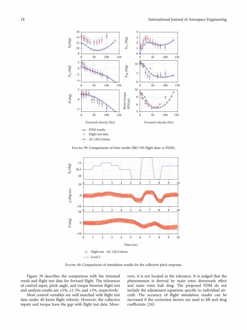
Figure 39 describes the comparison with the trimmedresult and flight test data for forward flight. The tolerancesof control input, pitch angle, and torque between flight testand analysis results are ±5%, ±1:5%, and ±3%, respectively.

Most control variables are well matched with flight testdata under 40 knots flight velocity. However, the collectiveinputs and torque have the gap with flight test data. More-

over, it is not located in the tolerance. It is judged that thephenomenon is derived by main rotor downwash effectand main rotor hub drag. The proposed FDM do notinclude the adjustment equations specific to individual air-craft. The accuracy of flight simulation results can beincreased if the correction factors are used to lift and dragcoefficients [24].

0 0

0

00

0

0

0

0

08

2

10121416

50 100 150

123

4

50

50

5050

50

100

100

100100

100

150

150

150150

150

5

5

–5

–4

–2

10

10

8

6

4

Forward velocity (Kn) Forward velocity (Kn)

FDM resultsFlight test dataAC 120 Criteria

𝜃 (d

eg)

𝛿1S

(deg

)𝛿

0(de

g)

Roto

r tor

que

(KN

/m)

δ TR

(deg

)δ 1

C (d

eg)

Figure 39: Comparisons of trim results (BO-105 flight data vs FDM).

0

0

0

0

0

10

10

10.5

10

–10

–10

11

1

1

1

2

2

2

3

3

3

4

4

4

5

5

5

6

6

6

7

7

7

8

8

8

9

9

9

10

10

10

Time (sec)

Flight test - AC 120 CriteriaLevel 2

𝜃 (d

eg)

δ 0 (d

eg)

q (d

eg/s

ec)

Figure 40: Comparisons of simulation results for the collective pitch response.


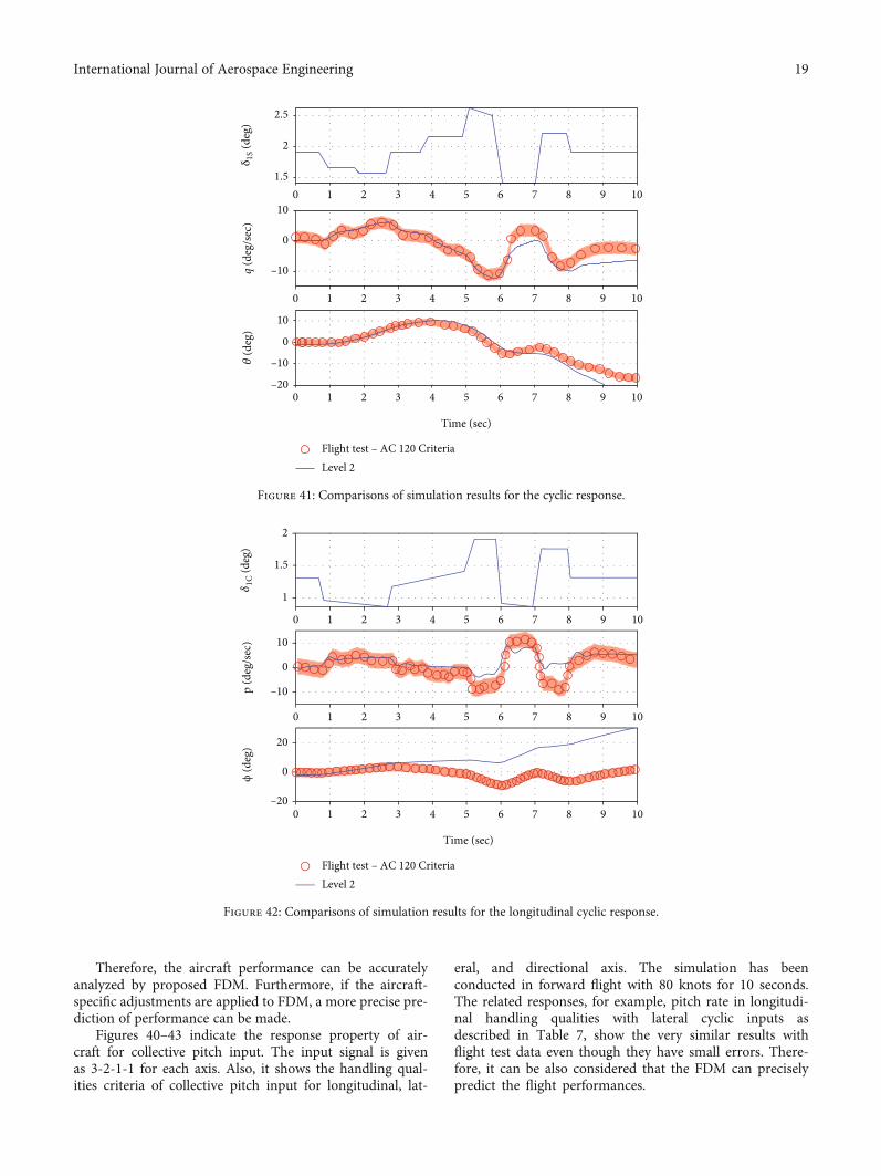
Therefore, the aircraft performance can be accuratelyanalyzed by proposed FDM. Furthermore, if the aircraft-specific adjustments are applied to FDM, a more precise pre-diction of performance can be made.

Figures 40–43 indicate the response property of air-craft for collective pitch input. The input signal is givenas 3-2-1-1 for each axis. Also, it shows the handling qual-ities criteria of collective pitch input for longitudinal, lat-

eral, and directional axis. The simulation has beenconducted in forward flight with 80 knots for 10 seconds.The related responses, for example, pitch rate in longitudi-nal handling qualities with lateral cyclic inputs asdescribed in Table 7, show the very similar results withflight test data even though they have small errors. There-fore, it can be also considered that the FDM can preciselypredict the flight performances.

2.5

1.5

2

0

0

0

0

0

1

1

1

2

2

2

3

3

3

4

4

4

5

5

5

6

6

6

7

7

7

8

8

8

9

9

9

10

10

10–20

–10

–10

10

10

Time (sec)

Flight test – AC 120 CriteriaLevel 2

𝜃 (d

eg)

q (d

eg/s

ec)

δ 1S (

deg)

Figure 41: Comparisons of simulation results for the cyclic response.

1.5

2

1

0

0

0

0

0

1

1

1

2

2

2

3

3

3

4

4

4

5

5

5

6

6

6

7

7

7

8

8

8

9 10

9

9

10

10

Time (sec)


–20

20

–10

10

ϕ (d

eg)

p (d

eg/s

ec)

𝛿1C

(deg

)

Figure 42: Comparisons of simulation results for the longitudinal cyclic response.


3.4. Compound Helicopter. The flight performance analysishas been carried out for a compound rotorcraft configurationto verify the usefulness of the FDM. The configuration ofcompound rotorcraft has been shown in Figure 44.

The compound aircraft using coaxial rotor is based onthe single rotor helicopter used in HETLAS. The coaxialrotors were assumed to be ABC rotors, and the blade chordswere adjusted to have the same solidity. In addition, the

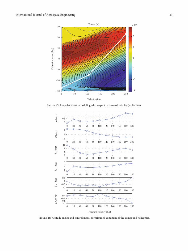
wings were attached to the center at both sides of the fuselage,and a pusher propeller was attached to the rear fuselage. Thecontrol inputs were collective, longitudinal and lateral cyclicpitches, and differential collective pitch as given in Equation(27). Furthermore, the collective control of the pusher wasapplied through thrust scheduling as shown in Figure 45 tocreate appropriate propulsive force according to the forwardflight velocity.

u = δ0, δ1C , δ1S, Δδ0ð ÞT : ð27Þ

Figures 46 shows the trim results of compound aircraft.The compound aircraft has a high pitch attitude angle withsmall roll attitude angle and lateral cyclic input due to torquefrom the pusher at the hovering status.

Then, the collective input is getting decreased with thepitch angle until 80 knots because of the lift of wing


1 20 3 4 5 6 7 8 9 10

20

–20

20

–20

4

3

2

r(de

g/se

c)𝛿TR(deg)

ψ (d

eg)

Time (sec)

1 20 3 4 5 6 7 8 9 10

1 20 3 4 5 6 7 8 9 10

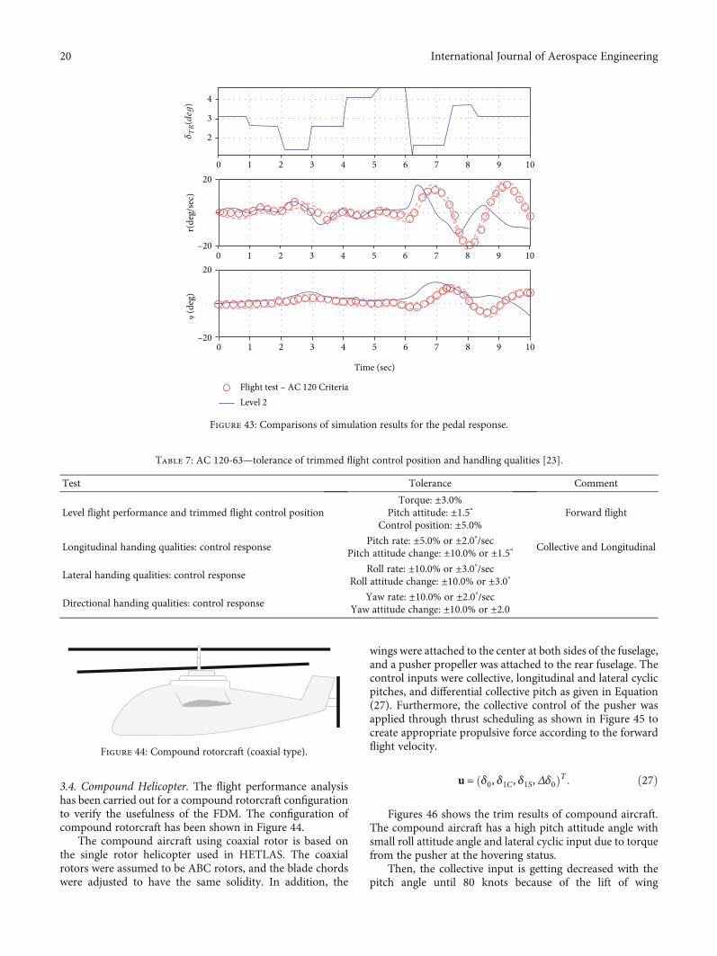
Figure 43: Comparisons of simulation results for the pedal response.

Table 7: AC 120-63—tolerance of trimmed flight control position and handling qualities [23].

Test Tolerance Comment

Level flight performance and trimmed flight control positionTorque: ±3.0%

Pitch attitude: ±1.5°Control position: ±5.0%

Forward flight

Longitudinal handing qualities: control responsePitch rate: ±5.0% or ±2.0°/sec

Pitch attitude change: ±10.0% or ±1.5° Collective and Longitudinal

Lateral handing qualities: control responseRoll rate: ±10.0% or ±3.0°/sec

Roll attitude change: ±10.0% or ±3.0°

Directional handing qualities: control responseYaw rate: ±10.0% or ±2.0°/sec

Yaw attitude change: ±10.0% or ±2.0

Figure 44: Compound rotorcraft (coaxial type).


Velocity (kn)

Colle

ctiv

e inp

ut (d

eg)

�rust (N)

0 50 100 150 200 250–30

–20

–10

0

10

20

30

–2

–1

0

1

2

3

x 104

Figure 45: Propeller thrust scheduling with respect to forward velocity (white line).

10.5

20

20

20

20

20

20

10

40

40

40

40

40

40

60

60

60

60

60

60

80

80

80

80

80

80

100

100

100

100

100

100

120

120

120

120

120

120

140

140

140

140

140

140

160

160

160

160

160

160

180

180

180

180

180

180

200

200

200

200

200

200

0

0

0

0

0

0

0

0

0

0

–5

–0.5

–0.4–0.6–0.8

–1

–1

0.5

5

987

Forward velocity (Kn)

2

4

ϕ (d

eg)

𝜃 (d

eg)

𝛿0 (

deg)

Δ𝛿

0 (de

g)𝛿

1C (d

eg)

𝛿1S

(deg

)

Figure 46: Attitude angles and control inputs for trimmed condition of the compound helicopter.


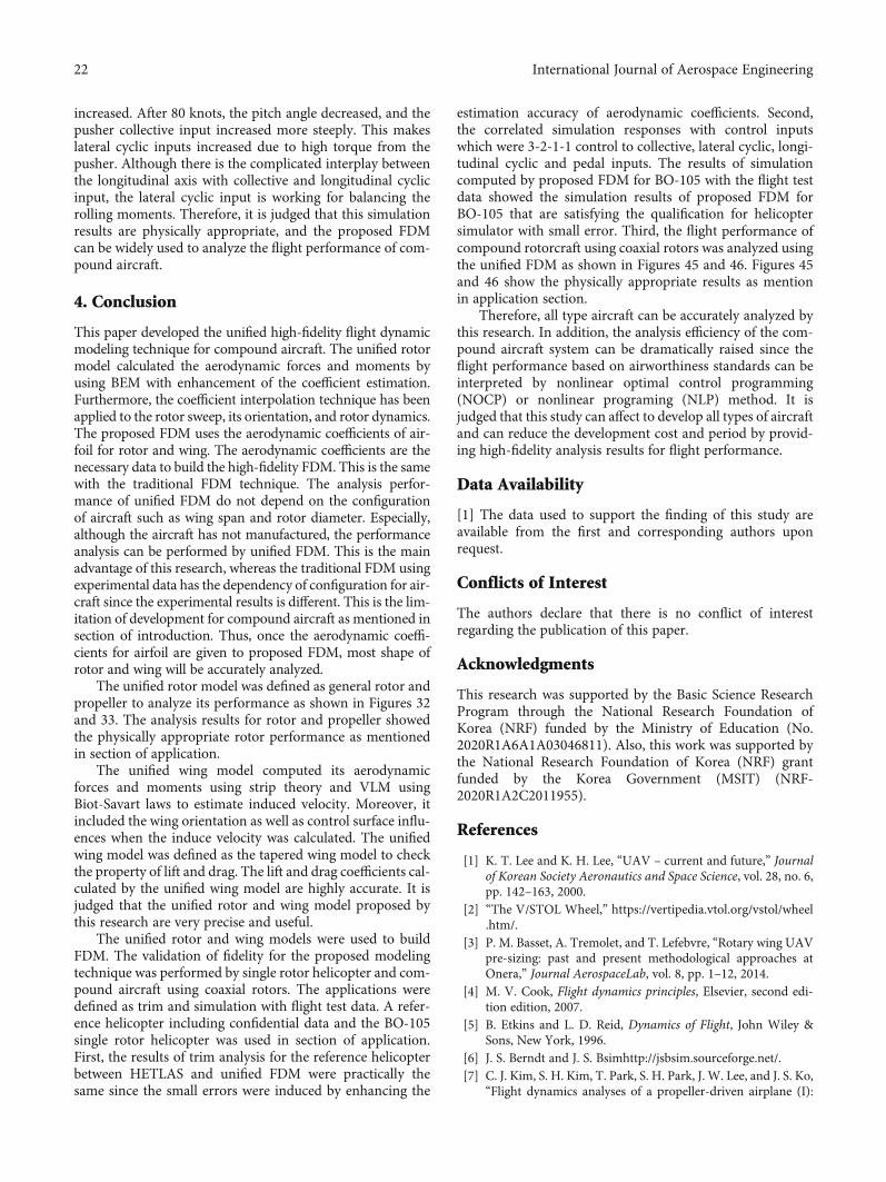
increased. After 80 knots, the pitch angle decreased, and thepusher collective input increased more steeply. This makeslateral cyclic inputs increased due to high torque from thepusher. Although there is the complicated interplay betweenthe longitudinal axis with collective and longitudinal cyclicinput, the lateral cyclic input is working for balancing therolling moments. Therefore, it is judged that this simulationresults are physically appropriate, and the proposed FDMcan be widely used to analyze the flight performance of com-pound aircraft.

4. Conclusion

This paper developed the unified high-fidelity flight dynamicmodeling technique for compound aircraft. The unified rotormodel calculated the aerodynamic forces and moments byusing BEM with enhancement of the coefficient estimation.Furthermore, the coefficient interpolation technique has beenapplied to the rotor sweep, its orientation, and rotor dynamics.The proposed FDM uses the aerodynamic coefficients of air-foil for rotor and wing. The aerodynamic coefficients are thenecessary data to build the high-fidelity FDM. This is the samewith the traditional FDM technique. The analysis perfor-mance of unified FDM do not depend on the configurationof aircraft such as wing span and rotor diameter. Especially,although the aircraft has not manufactured, the performanceanalysis can be performed by unified FDM. This is the mainadvantage of this research, whereas the traditional FDM usingexperimental data has the dependency of configuration for air-craft since the experimental results is different. This is the lim-itation of development for compound aircraft as mentioned insection of introduction. Thus, once the aerodynamic coeffi-cients for airfoil are given to proposed FDM, most shape ofrotor and wing will be accurately analyzed.

The unified rotor model was defined as general rotor andpropeller to analyze its performance as shown in Figures 32and 33. The analysis results for rotor and propeller showedthe physically appropriate rotor performance as mentionedin section of application.

The unified wing model computed its aerodynamicforces and moments using strip theory and VLM usingBiot-Savart laws to estimate induced velocity. Moreover, itincluded the wing orientation as well as control surface influ-ences when the induce velocity was calculated. The unifiedwing model was defined as the tapered wing model to checkthe property of lift and drag. The lift and drag coefficients cal-culated by the unified wing model are highly accurate. It isjudged that the unified rotor and wing model proposed bythis research are very precise and useful.

The unified rotor and wing models were used to buildFDM. The validation of fidelity for the proposed modelingtechnique was performed by single rotor helicopter and com-pound aircraft using coaxial rotors. The applications weredefined as trim and simulation with flight test data. A refer-ence helicopter including confidential data and the BO-105single rotor helicopter was used in section of application.First, the results of trim analysis for the reference helicopterbetween HETLAS and unified FDM were practically thesame since the small errors were induced by enhancing the

estimation accuracy of aerodynamic coefficients. Second,the correlated simulation responses with control inputswhich were 3-2-1-1 control to collective, lateral cyclic, longi-tudinal cyclic and pedal inputs. The results of simulationcomputed by proposed FDM for BO-105 with the flight testdata showed the simulation results of proposed FDM forBO-105 that are satisfying the qualification for helicoptersimulator with small error. Third, the flight performance ofcompound rotorcraft using coaxial rotors was analyzed usingthe unified FDM as shown in Figures 45 and 46. Figures 45and 46 show the physically appropriate results as mentionin application section.

Therefore, all type aircraft can be accurately analyzed bythis research. In addition, the analysis efficiency of the com-pound aircraft system can be dramatically raised since theflight performance based on airworthiness standards can beinterpreted by nonlinear optimal control programming(NOCP) or nonlinear programing (NLP) method. It isjudged that this study can affect to develop all types of aircraftand can reduce the development cost and period by provid-ing high-fidelity analysis results for flight performance.

Data Availability

[1] The data used to support the finding of this study areavailable from the first and corresponding authors uponrequest.

Conflicts of Interest

The authors declare that there is no conflict of interestregarding the publication of this paper.

Acknowledgments

This research was supported by the Basic Science ResearchProgram through the National Research Foundation ofKorea (NRF) funded by the Ministry of Education (No.2020R1A6A1A03046811). Also, this work was supported bythe National Research Foundation of Korea (NRF) grantfunded by the Korea Government (MSIT) (NRF-2020R1A2C2011955).

References

[1] K. T. Lee and K. H. Lee, “UAV – current and future,” Journalof Korean Society Aeronautics and Space Science, vol. 28, no. 6,pp. 142–163, 2000.

[2] “The V/STOL Wheel,” https://vertipedia.vtol.org/vstol/wheel.htm/.

[3] P. M. Basset, A. Tremolet, and T. Lefebvre, “Rotary wing UAVpre-sizing: past and present methodological approaches atOnera,” Journal AerospaceLab, vol. 8, pp. 1–12, 2014.

[4] M. V. Cook, Flight dynamics principles, Elsevier, second edi-tion edition, 2007.

[5] B. Etkins and L. D. Reid, Dynamics of Flight, John Wiley &Sons, New York, 1996.

[6] J. S. Berndt and J. S. Bsimhttp://jsbsim.sourceforge.net/.[7] C. J. Kim, S. H. Kim, T. Park, S. H. Park, J. W. Lee, and J. S. Ko,

“Flight dynamics analyses of a propeller-driven airplane (I):


https://vertipedia.vtol.org/vstol/wheel.htm/

https://vertipedia.vtol.org/vstol/wheel.htm/

http://jsbsim.sourceforge.net/

aerodynamic and inertial modeling of the propeller,” Interna-tional Journal of Aeronautics and Space Science, vol. 15, no. 4,pp. 345–355, 2014.

[8] J. Leishman, “Principles of helicopter aerodynamics,” in Partof Cambridge Aerospace Series, Cambridge university press,2nd edition edition, 2006.

[9] M. S. Chaffin, “A guide to the use of the pressure disk rotormodel as implemented in INS3D-UP,” National Aeronauticsand Space Administration, Technical Report NASA, vol. CR-4692, 1995.

[10] S. Taamallah, “Flight dynamics modeling for a small-scale fly-barless helicopter UAV,” in AIAA Atmospheric Flight Mechan-ics Conference, Portland, Oregon, 2011.

[11] J. Howlett, “UH-60A black hawk engineering simulation pro-gram: volume 1: mathematical model,” National Aeronauticsand Space Administration, vol. CR-166309, 1981.

[12] H. A. Pearson and R. F. Anderson, “Calculation of the aerody-namic characteristics of tapered wings with partial-span flaps,”Natinoal Advisory Committee for Aeronautics, vol. 665, 1939.

[13] P. D. Talbot, B. E. Tinling, W. A. Decker, and R. T. Chen, “Amathematical model of a single main rotor helicopter forpiloted simulation,” National Aeronautics and Space Adminis-tration, no. article TM84281, 1982.

[14] R. J. Ruddell, “Advancing blade concept (ABC) technologydemonstrator,” Defense Technical Information Center,USAAVRDCOM-TR-81-D-5, 1981.

[15] C. J. Kim, “Implicit formulation of rotor aeromechanic equa-tions for helicopter flight simulation,” Journal of the KoreanSociety for Aeronautical and Space Science, vol. 30, no. 3,pp. 8–16, 2002.

[16] D. H. Lee, Design of the Control System to Implement theAutonomous Tactical Maneuvers of the Fixed-Wing Aircraft,Konkuk University, 2019.

[17] R. Fink, USAF Stability and Control DATCOM, AFWAL-TR-83-3048, 1978.

[18] Y. H. Yun, C. D. Yang, C. J. Kim, and I. J. Cho, “Flight dynamicanalysis program, HETLAS for development of helicopterFBW,” in Korean Society for Aeronautical & Space Sciences2012 Spring Conference, pp. 1270–1275, Jeju, 2012.

[19] https://ko.wikipedia.org/wiki/KAI_%EC%88%98%EB%A6%AC%EC%98%A8/.

[20] http://www.rotorleasing.com/Specifications/BO105.html/.

[21] S. H. Lee, D. H. Lee, S. H. Hur, S. H. Kang, and C. J. Kim, “Gen-eral methods of rotor and wing aerodynamics modeling fordrone/UAV flight dynamic model,” in Korean Society forAeronautical & Space Sciences 2017 Spring Conference,pp. 666-667, Samcheok, Gangwon, 2017.

[22] J. Wan, Ornicopter Multidisciplinary Analyses and ConceptualDesign, Delft University of Technology, 2014.

[23] “Helicopter Simulator Qualification,” in FAA Advisory Circu-lar AC 120-63, Federal Aviation Authority, 1994.

[24] M. Kerler, J. Honle, and H.-P. Kau, Modeling of BO 105 FlightDynamics for Research on Fuel Savings due to Single-EngineOperation, 38th European Rotorcraft Forum, Amsterdam,2012.


https://ko.wikipedia.org/wiki/KAI_%EC%88%98%EB%A6%AC%EC%98%A8/

https://ko.wikipedia.org/wiki/KAI_%EC%88%98%EB%A6%AC%EC%98%A8/

http://www.rotorleasing.com/Specifications/BO105.html/

Documents

Development of Unified High-Fidelity Flight Dynamic