Embed Size (px)
Citation preview

i
DEVELOPMENT OF ULTRASOUND IMAGE CONTRAST
ENHANCEMENT AND SPECKLE NOISE REDUCTION FOR KNEE
OSTEOARTHRITIS EARLY DETECTION
MD BELAYET HOSSAIN
DISSERTATION SUBMITTED IN PARTIAL FULFILLMENT OF THE
REQUIREMENTS FOR THE DEGREE OF MASTER OF
ENGINEERING
DEPARTMENT OF BIOMEDICAL ENGINEERING
FACULTY OF ENGINEERING
UNIVERSITY MALAYA
KUALA LUMPUR
2014
ii
UNIVERSITY MALAYA
ORIGINAL LITERARY WORK DECLARATION
Name of Candidate: Md Belayet Hossain Passport No:
Registration/Matric No: KGA120044
Name of Degree: Master of Engineering Science
Title of Project Paper/ Research Report/ Dissertation/ Thesis (“This Work”):
Development of Ultrasound Image Contrast Enhancement and Speckle Noise Reduction for
Knee Osteoarthritis Early Detection.
Field of Study: Biomedical Imaging
I do solemnly and sincerely declare that:
(1) I am the sole author/writer of this Work;
(2) This work is original;
(3) Any use of any work in which copyright exists was done by way of fair dealing and for
permitted purpose and any excerpt from, or reference to or reproduction of any copyright
work has been disclose expressly and sufficiently and the title of the Work and its
authorship have been acknowledge in this Work;
(4) I do not have any actual knowledge nor do I ought reasonably to know that the making of
this work constitutes an infringement of any copyright work;
(5) I hereby assign all and every rights in the copyright to this work to the University of
Malaya (UM), who henceforth shall be owner of the copyright in this work and that any
written consent of UM having been first had and obtained;
(6) I am fully aware that if in the course of making this work I have infringed any copyright
whether intentionally or otherwise, I am be subject to legal action or any other action as
may be determined by UM.
Candidate’s Signature Date:
Subscribed and solemnly declared before,
Witness’s Signature Date:
Name:
Designation:

iii
ABSTRAK
Lutut Osteoartritis (OA) adalah salah satu penyakit yang paling biasa di kalangan warga tua.
Biasanya, rawatan perubatan tidak diutamakan sehingga penyakit itu telah berkembang ke titik
di mana ia tidak mungkin didiagnosis secara berkesan. Hal ini sering disebabkan oleh
kebimbangan terhadap kos pengesanan semasa peringkat awal. Ultrasound (US) pengimejan
mempunyai beberapa kelebihan sebagai teknik pengimejan. Ia merupakan satu kaedah
diagnostik yang kos rendah, tidak invasif, tidak mengionkan dan dapat menyediakan visualisasi
yang intuitif. Terdapat perubahan yang ketara dalam bentuk rawan kerana perkembangan OA
yang berkiat dengan degenerasi tulang rawan. Dengan menggunakan pengimejan US, ia dapat
mengesan penyempitan ruang lutut. Namun, nisbah kontras yang rendah dan bunyi belu yang
menghadkan penggunaan produk ini. Objektif tesis ini adalah untuk mencadangkan cara baru
yang dapat menambahkan kostras dan mengurangkan beru yang akan mengatasi had-had
tersebut. Dalam kaedah yang dicadangkan itu, peningkatan nilai-nilai optimum kontras,
kecerahan dan pemeliharaan terperinci akan diambil kira. Kebanyakan kaedah peningkatan
konvensional hanya menekankan satu watak manakala kaedah yang dicadangkan melibatkan
penubuhan titik pemisah di segmen histogram untuk kontras optimum, kecerahan dan
pemeliharaan terperinci dalam masa yang sama. Tiga metrik akan digunakan dalam
pengoptimuman ini, iaitu Pemeliharaan Fungsi Skor Kecerahan (PBS), Fungsi Kontras Skor
Optimum (OCS), dan Pemeliharaan Fungsi Skor Terperinci (PDS) ditakrifkan. Untuk
mengurangkan bunyi belu dan mengekalkan ciri-ciri kelebihannya, fungsi kemeresapan baru
dan kecerunan empat ambang digunakan dan bukan satu. Untuk menganalisis prestasi, analisis
kuantitatif dan kualitatif telah dijalankan dengan menggunakan kedua-dua imej ultrasound
sintetik dan nyata. Keputusan membuktikan bahawa kaedah yang dicadangkan melebihi kaedah
yang sedia ada.
iv
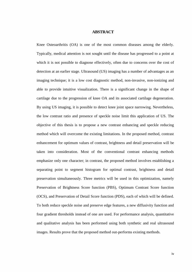
ABSTRACT
Knee Osteoarthritis (OA) is one of the most common diseases among the elderly.
Typically, medical attention is not sought until the disease has progressed to a point at
which it is not possible to diagnose effectively, often due to concerns over the cost of
detection at an earlier stage. Ultrasound (US) imaging has a number of advantages as an
imaging technique; it is a low cost diagnostic method, non-invasive, non-ionizing and
able to provide intuitive visualization. There is a significant change in the shape of
cartilage due to the progression of knee OA and its associated cartilage degeneration.
By using US imaging, it is possible to detect knee joint space narrowing. Nevertheless,
the low contrast ratio and presence of speckle noise limit this application of US. The
objective of this thesis is to propose a new contrast enhancing and speckle reducing
method which will overcome the existing limitations. In the proposed method, contrast
enhancement for optimum values of contrast, brightness and detail preservation will be
taken into consideration. Most of the conventional contrast enhancing methods
emphasize only one character; in contrast, the proposed method involves establishing a
separating point to segment histogram for optimal contrast, brightness and detail
preservation simultaneously. Three metrics will be used in this optimization, namely
Preservation of Brightness Score function (PBS), Optimum Contrast Score function
(OCS), and Preservation of Detail Score function (PDS), each of which will be defined.
To both reduce speckle noise and preserve edge features, a new diffusivity function and
four gradient thresholds instead of one are used. For performance analysis, quantitative
and qualitative analysis has been performed using both synthetic and real ultrasound
images. Results prove that the proposed method out-performs existing methods.

v
ACKNOWLEDGEMENT
With the deepest gratitude I wish to thank my beloved supervisor, Dr. Lai Khin Wee for
providing a define guidance and intellectual support. Dr. Belinda Murphy is willing to
spend her time to teach and explain to me whenever I encountered problems. Without
them, I would not be able to excel my projects successfully.
Secondly, I would like to acknowledge and express my gratitude to the Dr.
Dipankar Choudhury who has provided his idea for the project. Never forgetting to
thank Mr. Heamn and Prof. Dr. John George, who helped me a lot for collecting the US
images of knee joint.
Last but not least, I wish to express my appreciation to everyone who has come
into my life and inspired, touched, and illuminated me through their presence. I have
learned something from all of you to make my project a valuable as well as an enjoyable
one.
Thank you.

vi
TABLE OF CONTENTS
ORIGINAL LITERARY WORK DECLARATION ........................................................ ii
ABSTRAK ....................................................................................................................... iii
ABSTRACT ..................................................................................................................... iv
ACKNOWLEDGEMENT ................................................................................................ v
TABLE OF CONTENTS ................................................................................................. vi
LIST OF FIGURES ......................................................................................................... ix
LIST OF TABLES ........................................................................................................... xi
LIST OF SYMBOLS ..................................................................................................... xiii
LIST OF ABBREVIATIONS ........................................................................................ xiv
CHAPTER 1 ..................................................................................................................... 1
INTRODUCTION ............................................................................................................ 1
1.1 Background ........................................................................................................ 1
1.2 Significance of the study .................................................................................... 2
1.3 Problem Statement ............................................................................................. 4
1.4 Objectives ........................................................................................................... 6
1.5 Methodology ...................................................................................................... 7
1.6 Overview of each chapter ................................................................................... 8
1.6.1 Chapter 1 ..................................................................................................... 8
1.6.2 Chapter 2 ..................................................................................................... 8
1.6.3 Chapter 3 ..................................................................................................... 8
1.6.4 Chapter 4 ..................................................................................................... 9
1.6.5 Chapter 5 ..................................................................................................... 9
CHAPTER 2 ................................................................................................................... 10
LITERATURE REVIEW................................................................................................ 10
2.1 Background ...................................................................................................... 10
2.2 Different medical imaging system ................................................................... 10
2.2.1 Radiograph: X-Ray ................................................................................... 10
2.2.2 Computed Tomography (CT) .................................................................... 12
2.2.3 Magnetic Resonance Imaging (MRI) ........................................................ 12
2.2.4 Ultrasound ................................................................................................. 14
2.3 Procedure of US scanning protocol .................................................................. 16
vii
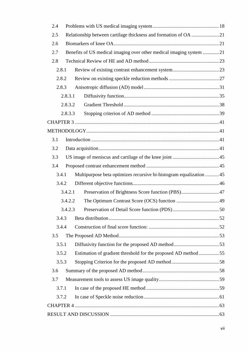
2.4 Problems with US medical imaging system ..................................................... 18
2.5 Relationship between cartilage thickness and formation of OA ...................... 21
2.6 Biomarkers of knee OA .................................................................................... 21
2.7 Benefits of US medical imaging over other medical imaging system ............. 21
2.8 Technical Review of HE and AD method ........................................................ 23
2.8.1 Review of existing contrast enhancement system ..................................... 23
2.8.2 Review on existing speckle reduction methods ........................................ 27
2.8.3 Anisotropic diffusion (AD) model ............................................................ 31
2.8.3.1 Diffusivity function............................................................................ 35
2.8.3.2 Gradient Threshold ............................................................................ 38
2.8.3.3 Stopping criterion of AD method ...................................................... 39
CHAPTER 3 ................................................................................................................... 41
METHODOLOGY .......................................................................................................... 41
3.1 Introduction ...................................................................................................... 41
3.2 Data acquisition ................................................................................................ 41
3.3 US image of meniscus and cartilage of the knee joint ..................................... 45
3.4 Proposed contrast enhancement method .......................................................... 45
3.4.1 Multipurpose beta optimizes recursive bi-histogram equalization ........... 45
3.4.2 Different objective functions..................................................................... 46
3.4.2.1 Preservation of Brightness Score function (PBS) .............................. 47
3.4.2.2 The Optimum Contrast Score (OCS) function .................................. 49
3.4.2.3 Preservation of Detail Score function (PDS) ..................................... 50
3.4.3 Beta distribution ........................................................................................ 52
3.4.4 Construction of final score function: ........................................................ 52
3.5 The Proposed AD Method ................................................................................ 53
3.5.1 Diffusivity function for the proposed AD method .................................... 53
3.5.2 Estimation of gradient threshold for the proposed AD method ................ 55
3.5.3 Stopping Criterion for the proposed AD method ...................................... 58
3.6 Summary of the proposed AD method ............................................................. 58
3.7 Measurement tools to assess US image quality ................................................ 59
3.7.1 In case of the proposed HE method .......................................................... 59
3.7.2 In case of Speckle noise reduction ............................................................ 61
CHAPTER 4 ................................................................................................................... 63
RESULT AND DISCUSSION ....................................................................................... 63

viii
4.1 Introduction ...................................................................................................... 63
4.2 For proposed contrast enhancement method .................................................... 64
4.2.1 Qualitative analysis ................................................................................... 64
4.2.1.1 Text on Cartilage Image .................................................................... 64
4.2.1.2 Test on meniscus Image ..................................................................... 66
4.2.2 Quantitative analysis ................................................................................. 70
4.2.2.1 Histogram equalization ...................................................................... 78
4.2.2.2 Mean shift .......................................................................................... 79
4.2.2.3 Graph by entropy ............................................................................... 80
4.3 For proposed AD method ................................................................................. 81
4.3.1 Qualitative analysis ................................................................................... 81
4.3.1.1 Test on cartilage Image ...................................................................... 84
4.3.1.2 Test on Meniscus Image .................................................................... 85
4.3.2 Quantitative analysis ................................................................................. 87
CHAPTER 5 ................................................................................................................... 92
CONCLUSION AND FUTURE WORK ....................................................................... 92
5.1 Conclusion ........................................................................................................ 92
5.2 Limitation of the proposed method .................................................................. 93
5.3 Future work ...................................................................................................... 94
REFERENCES ................................................................................................................ 95
SUPPLEMENTARY .................................................................................................... 103
LIST OF PUBLICATIONS AND PAPERS PRESENTED ......................................... 103
APPENDIX ................................................................................................................... 103

ix
LIST OF FIGURES
Figure 1.1: Flowchart of research Activities ..................................................................... 7
Figure 2.1 X-ray image of right knee .............................................................................. 11
Figure 2.2 C.T. image of right knee ................................................................................ 12
Figure 2.3 MRI image of right knee ............................................................................... 14
Figure 2.4 US image of right knee .................................................................................. 16
Figure 2.5 Procedure of Image scanning by US machine ............................................... 18
Figure 2.6 Three flow functions are scaled so that maximum flow occur at the
same point at x=0.2 ......................................................................................................... 37
Figure 3.1: (a-g) is ultrasound images of knee joint Cartilage collected from
UTM (Healthy subjects) .................................................................................................. 43
Figure 3.2: (a-g) is ultrasound image of knee joint Meniscus collected from
UMMC (Healthy subjects) .............................................................................................. 44
Figure 3.3 Knee joint of a normal knee........................................................................... 45
Figure 3.4: The flow function ɸ2 and ɸ3 are scaled so that the value of ɸ2 is
near zero at x=0.4 where it is zero for ɸ3 ....................................................................... 55
Figure 3.5 C is the central pixel of [3×3] mask and (a)Four pixels of four
directions has been considered (b) Eight pixels of eight directions has been
considered ....................................................................................................................... 56
Figure 4.1: .(a) Original Cartilage Image (b) Conventional HE (c) BBHE
(d) DSIHE (e) RSIHE (f) MMBEBHE (g) MBORBHE (proposed) .............................. 66
Figure 4.2: (a) Original Image (b) Conventional HE (c) BBHE (d)DSIHE
(e) RSIHE (f)MMBEBHE (g) MBORBHE (proposed). (In case of meniscus
image) .............................................................................................................................. 68
Figure 4.3: US images of knee Meniscus for four subjects before and after
contrast enhancement are shown above (a), (b) are input and output image
for subject 1. (c), (d) are input and output image for subject 2. (e), (f) are input
and output image for subject 3, (g), (h) are input and output image for subject 4 .......... 69
Figure 4.4: (a), (b) and (c) denote the Histogram of US images of knee
joint cartilage for original, HE based and proposed method respectively ...................... 77
Figure 4.5: (a), (b) and (c) denote the Histogram of US images of knee
joint meniscus for original, HE based and proposed method respectively ..................... 78
Figure 4.6: Mean of original, HE and Proposed HE method .......................................... 79

x
Figure 4.7: Entropy for conventional HE and proposed HE method for two
images ............................................................................................................................. 80
Figure 4.8: (a) original image. (b) Simulated ultrasound image (c) AD
filtering using g2 after 30 iterations (d) AD filtering using g3 after 30 iteration ........... 82
Figure 4.9: (a) Portion of seismic image. (b) Filtered version with estimated one
gradient threshold S after 10 iterations. (c) Filtered version with estimated two
gradient threshold after 10 iterations. (d) Filtered version with estimated four
gradient threshold ............................................................................................................ 83
Figure 4.10: The estimation of one gradient threshold parameter S, two gradient
threshold parameters SNS, SEW, and estimation of four threshold parameters
SWNSE and SNEWS of Fig. 4.9 in every iteration with the help of knee
algorithm ......................................................................................................................... 83
Figure 4.11: US Image of Cartilage for AD (a) Original Image. Resultant
image of AD filtered image by using (b) Perona Malik method (c) SRAD
method (d) Non-Linear Complex Diffusion method (NCD) (e) LPND
(f) proposed method. ....................................................................................................... 85
Figure 4.12: US image of cartilage for medial side of knee joint for AD
(a) Original Image. Resultant image of AD filter by using (b) Perona Malik
method (c) SRAD method (d) Non-Linear Complex Diffusion method (NCD)
(e) LPND (f) Proposed method. ...................................................................................... 86

xi
LIST OF TABLES
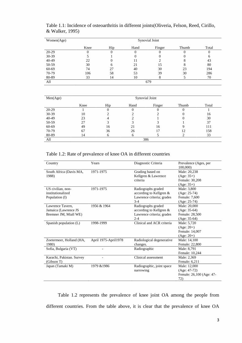
Table 1.1: Incidence of osteoarthritis in different joints(Oliveria, Felson, Reed,
Cirillo, & Walker, 1995) ................................................................................................... 3
Table 1.2: Rate of prevalence of knee OA in different countries ..................................... 3
Table 2.1 Comparison of different medical imaging for OA assessment ....................... 16
Table 4.1: Mean value of SNR, SSIM and Entropy for different contrast
enhancement methods ..................................................................................................... 71
Table 4.2: The one-way ANOVA test by using different contrast enhancement
methods in SNR, SSIM and Entropy .............................................................................. 71
Table 4.3: Categorization of different methods using Fisher’s Least Significant
Difference (LSD) for SNR .............................................................................................. 72
Table 4.4: Categorization of contrast enhancement methods into homogenous
subset using the Duncan test for SNR ............................................................................. 72
Table 4.5: Categorization of different methods using Fisher’s Least Significant
Difference (LSD) for SSIM ............................................................................................ 73
Table 4.6: Categorization of contrast enhancement methods into homogenous
subset using the Duncan test for SSIM ........................................................................... 74
Table 4.7: Categorization of different methods using Fisher’s Least Significance
Difference (LSD) for Entropy ......................................................................................... 74
Table 4.8: Categorization of contrast enhancement methods into homogenous
subset using Duncan test for Entropy ............................................................................. 75
Table 4.9: Ranking of different contrast enhancement methods in terms of
SNR, SSIM and Entropy. The methods ranking has been computed according
to Fisher’s Least Significant Difference (LSD) and the Duncan test.............................. 76
Table 4.10: Mean value of PSNR, SSIM and FOM with standard deviation for
PM, LPND, NCD, SRAD and proposed method ............................................................ 87
Table 4.11: The one-way ANOVA computed by using different speckle reduction
methods in PSNR, FOM and SSIM ................................................................................ 87
Table 4.12: Categorization of different methods using Fisher’s Least Significance
Difference (LSD) for PSNR ............................................................................................ 88
Table 4.13: Categorization of speckle reduction methods into homogenous subset
using the Duncan test for PSNR...................................................................................... 89

xii
Table 4.14: Categorization of different methods using Fisher’s Least Significant
Difference (LSD) for FOM ............................................................................................. 89
Table 4.15: Categorization of speckle reduction methods into homogenous subset
using the Duncan test for FOM ....................................................................................... 90
Table 4.16: Categorization of different methods using Fisher’s Least Significance
Difference (LSD) for SSIM ............................................................................................ 90
Table 4.17: Categorization of speckle reduction methods into homogenous subset
using Duncan’s test for SSIM ......................................................................................... 91
Table 4.18: Ranking of methods in terms of peak PSNR, SSIM and FOM. The
method ranking is computed according to Fisher’s Least Significance Difference
(LSD) and the Duncan test. ............................................................................................. 91

xiii
LIST OF SYMBOLS
* Convolution
C Constant for Stabilizing Equation
Λ Diffusion Control Rate
G Diffusivity Function
Δ Difference of pixels by using mask
S Estimated Gradient Threshold
D Euclidian distance
G(σ) Gaussian kernel function
ɸ Generated Brightness Flow
𝛁 Gradient Operator
µx Mean Brightness of Input Image
µy Mean Brightness Output Image
σx Normalized Root Mean Square contrast of the input image
σy Normalized Root Mean Square contrast of the output image
R Number of Recursion of HE methods
I0 Original Image
It Output image after t iterations
ηs Spatial pixel neighborhood
Σ Standard Deviation
α, β, ɸ Shape parameters

xiv
LIST OF ABBREVIATIONS
AD Anisotropic Diffusion
ASD Average Structural Difference
AMBE Absolute Mean Brightness Error
ASSF Adaptive Speckle Suppression Filter
AWMF Adaptive Weighted Median Filter
BBHE Brightness Preserving Bi-Histogram Equalization
CS Contrast Score
CT Computed Tomography
CEDU Contrast Enhancement Diagnostic Ultrasound
DSIHE Dualistic sub-image histogram equalization
E East
Ent Entropy
EPS Edge Preservation Score Function
FSE Fast-Spin Echo
FP False Positive
FN False Negative
FOM Figure of Merits
HE Histogram Equalization
JSN Joint Space Narrowing
MAE Mean Absolute Error
MRI Magnetic Resonance Imaging
MSE Mean Square Error
MMBEBHE Minimum Mean Brightness Error bio-Histogram Equalization
MMSE Minimum Mean Square Error
MBORBHE Multipurpose Beta Optimized Recursive Bi-Histogram Equalization

xv
N North
NB Normalized Brightness
NC Normalized Contrast
ND Normalized Detail
NCS Normalized Contrast Score
NPDS Normalized Preservation of Detail Score
NPBS Normalized Preservation of Brightness Score
NCD Nonlinear Complex Diffusion
ND Normalized Detail
NE North-East
NLM Non Local Mean
NPV Negative Predictive Values
NOCS Normalized Optimum Contrast Score Function
NRMS Normalized Root Mean Square
OA Osteoarthritis
OCS Optimum Contrast Score function
PBS Preservation of Brightness Score function
PDF Probability Density Function
PD Proton density
PDS Preservation of Detail Score function
PES Preservation of Edge Score
PM Perona-Malik
PPV Positive Predictive Values
PSNR Peak Signal to Noise Ratio
RF Radio Frequency
RMSHE Recursive Mean Separate Histogram Equalization

xvi
RSIHE Recursive sub-image histogram equalization
RLBHE Range Limited Bi-Histogram Equalization
RSWHE Recursive Separated and Weighted Histogram Equalization
S South
SE South-East
SNR Signal to Noise Ratio
SRAD Speckle Reducing Anisotropic Diffusion
SRHE Sub Region Histogram Equalization
SSIM Structure Similarity Index Measurement
TP True Positive
TN True Negative
US Ultrasound
USG Ultrasonography System
W West
WN West-North
WS West-South
WTHE Weighted Threshold HE
WCHE Wight Clustering Histogram Equalization
1
CHAPTER 1
INTRODUCTION
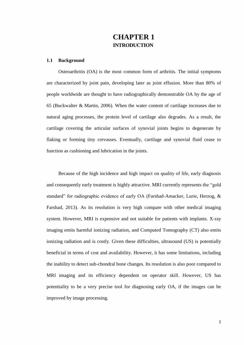
1.1 Background
Osteoarthritis (OA) is the most common form of arthritis. The initial symptoms
are characterized by joint pain, developing later as joint effusion. More than 80% of
people worldwide are thought to have radiographically demonstrable OA by the age of
65 (Buckwalter & Martin, 2006). When the water content of cartilage increases due to
natural aging processes, the protein level of cartilage also degrades. As a result, the
cartilage covering the articular surfaces of synovial joints begins to degenerate by
flaking or forming tiny crevasses. Eventually, cartilage and synovial fluid cease to
function as cushioning and lubrication in the joints.
Because of the high incidence and high impact on quality of life, early diagnosis
and consequently early treatment is highly attractive. MRI currently represents the “gold
standard” for radiographic evidence of early OA (Farshad-Amacker, Lurie, Herzog, &
Farshad, 2013). As its resolution is very high compare with other medical imaging
system. However, MRI is expensive and not suitable for patients with implants. X-ray
imaging emits harmful ionizing radiation, and Computed Tomography (CT) also emits
ionizing radiation and is costly. Given these difficulties, ultrasound (US) is potentially
beneficial in terms of cost and availability. However, it has some limitations, including
the inability to detect sub-chondral bone changes. Its resolution is also poor compared to
MRI imaging and its efficiency dependent on operator skill. However, US has
potentiality to be a very precise tool for diagnosing early OA, if the images can be
improved by image processing.

2
Therefore, the aim of this thesis is to improve US image processing so that US
can be utilized for the early diagnosis of knee OA. In this thesis, US images of knee
joint cartilage and meniscus, mainly collected from a male population, have been used
as test data. The outcome of the thesis will be a novel technique for obtaining
information on early OA by using Ultrasound Imaging.
1.2 Significance of the study
Presently, OA is a burden to one-third of adults worldwide, and the prevalence of
this disease is higher among the elderly people (Felson DT, 1987). Oliveria et al
(Oliveria SA) conducted a study to find the prevalence of OA among the people of a
health maintenance organization in Massachusetts, which has revealed that OA of the
knee is more prevalent than OA of other joints, and shown in the Table 1.1 Furthermore,
as Table 1.1 also shows clearly, OA disease is more common in women than men. The
prevalence of knee OA in different countries is also given in Table 1.2. Indeed, OA is
considered as a major burden to any health care system. The yearly financial cost of
knee OA and other arthritis is much higher than other chronic diseases. For example, for
the treatment of arthritis, around 95 billion USD per year is spent in the United States
("CDC. Public health and aging: Projected prevalence of self reported arthritis or
chronic joint symptoms among persons aged 65 years in United States, 2005-2030.,"
2003). The amount excludes the cost of lost employment opportunities of patients.
However, by using demographic prediction it is estimated that more than 20% of the
population having an age over 60 will be affected by knee osteoarthritis by 2040
(HamermanD, 1995).
3
Table 1.1: Incidence of osteoarthritis in different joints(Oliveria, Felson, Reed, Cirillo,
& Walker, 1995)
Women(Age) Synovial Joint
Knee Hip Hand Finger Thumb Total
20-29 0 0 0 0 0 0
30-39 5 1 0 0 0 6
40-49 22 0 11 2 8 43
50-59 30 6 21 15 8 80
60-69 74 27 40 30 23 194
70-79 106 58 53 39 30 286
80-89 33 14 10 8 5 70
All 679
Men(Age) Synovial Joint
Knee Hip Hand Finger Thumb Total
20-29 1 0 0 0 0 1
30-39 10 2 2 2 0 16
40-49 23 4 2 1 0 30
50-59 27 3 3 3 1 37
60-69 49 16 21 16 9 111
70-79 67 36 26 17 12 158
80-89 14 6 6 5 2 33
All 386
Table 1.2: Rate of prevalence of knee OA in different countries
Country Years Diagnostic Criteria Prevalence (Ages, per
100,000)
South Africa (Davis MA,
1988)
1971-1975 Grading based on
Kellgren & Lawrence
criteria
Male: 20,238
(Age: 35+)
Female: 30,208
(Age: 35+)
US civilian, non-
institutionalized
Population (I)
1971-1975 Radiographs graded
according to Kellgren &
Lawrence criteria; grades
3-4
Male: 3,800
(Age: 25-74)
Female: 7,600
(Age: 25-74)
Lawrence Tavern,
Jamaica (Lawrence JS
Bremner JM, Miall WE)
1956 & 1964 Radiographs graded
according to Kellgren &
Lawrence criteria; grades
2-4
Male: 20,000
(Age: 35-64)
Female: 28,500
(Age: 35-64)
Spanish population (L) 1998-1999 Clinical and ACR criteria Male: 5,720
(Age: 20+)
Female: 14,007
(Age: 20+)
Zoetermeer, Holland (HA,
1980)
April 1975-April1978 Radiological degenerative
changes.
Male: 14,100
Female: 22,800
Sofia, Bulgaria (VT) - Radiographic Male: 8,791
Female: 10,244
Karachi, Pakistan. Survey
(Gibson T)
- Clinical assessment Male: 2,369
Female: 6,211
Japan (Tamaki M) 1979 &1986 Radiographic, joint space
narrowing
Male: 12,000
(Age: 47-72)
Female: 26,100 (Age: 47-
72)
Table 1.2 represents the prevalence of knee joint OA among the people from
different countries. From the table above, it is clear that the prevalence of knee OA

4
among the women is higher than men. Most patients with early knee OA are reluctant to
seek a physician to obtain a diagnosis. This reluctance arises from the limited
availability of diagnostic facilities and high costs involved in many clinics. For
example, an MRI image costs about USD 280 in Malaysian public hospitals.
Conventional X-rays are more economic but not radiation free. CTs are expensive and
also use ionized radiation. However, US can overcome these limitations since it is
portable, radiation free, capable of generating a real time image, and also cost effective.
If the exponential increase of knee OA is to be reduced, it is necessary to detect early
knee OA. If this is possible, then the increased consequence of knee OA on world health
and economy may be partly averted.
1.3 Problem Statement
Although US imaging has a lot of advantages, including real time imaging, low
cost, intuitive visualization, and being non-invasive, it suffers from two drawbacks,
namely low contrast ratio and speckle noise which challenge the interpretation of image.
For that reason, an experienced radiologist is required to inspect US images to detect
early knee OA. To detect early OA using US is a big challenge for any radiologist or
sonographer. However, if US images can be processed so that their contrast ratio is
increased and speckle noise is reduced, then it will be more convenient for the early
detection of OA (Keen, Wakefield, & Conaghan, 2009). The reluctance to obtain
diagnosis of early knee OA could also be minimized since US images have a lot of
benefits over other medical imaging systems, including being radiation free, suitable for
a general clinical environment, painless, readily clinically accessible, low cost, non-
invasive, portable (A.B A.Achim, 2001; B.Sahiner, 2008; J.S. H.D.Cheng,
W.Ju,Y.Guo,L.Zhang, 2010) and bringing continuing improvement in the image
quality. Real time visualization is also possible by using ultrasound. Its low contrast

5
ratio can be ameliorated by using Histogram Equalization (HE) (Chen et al., 2005).
Likewise, speckle noise can be reduced by using anisotropic diffusion (AD)(Sun,
Hossack, Tang, & Acton, 2004).
For that reason assistance has been sought improve the conventional HE method
and anisotropic diffusion method to overcome their existing limitations. In the case of
the conventional HE method, selecting the appropriate separating point for segmenting
the histogram is the main challenge. By using the proposed HE method the optimum
separating point for segmenting the histogram will be selected, so that brightness and
detail preservation occur at the same time as contrast enhancement of the US image. For
obtaining the optimum separating point three objective functions will be considered,
namely Preservation of Brightness Score function (PBS), Optimum Contrast Score
function (OCS) and Preservation of Detail Score function (PDS). Different types of
artifact also make US images harder to interpret and to use in obtaining quantitative
information. Noise in US images can be divided into two main components; first,
thermal or electronic noise (additive noise), and second, multiplicative noise called
‘speckle’ (Achim, Bezerianos, & Tsakalides, 2001). Speckle is a random deterministic
interference pattern in an image which is formed with coherent radiation of a medium,
comprising of many sub-resolution scatterers. The superposition of acoustic echo
generates an intricate interference pattern as the US pulse randomly interferes with
objects of comparable size to the sound wavelength. Constructive and destructive
coherent summation of ultrasound echoes produces speckle (Burckhardt, 1978). The
undesirable consequence of the US image formation process in coherent US image is
the speckle noise. This formation of speckle has a great impact on the US image, and
leads to diagnostically important features of the US image being greatly deteriorated,
and a subsequent lack of accuracy in the diagnosis of disease. For accurate diagnosis, it
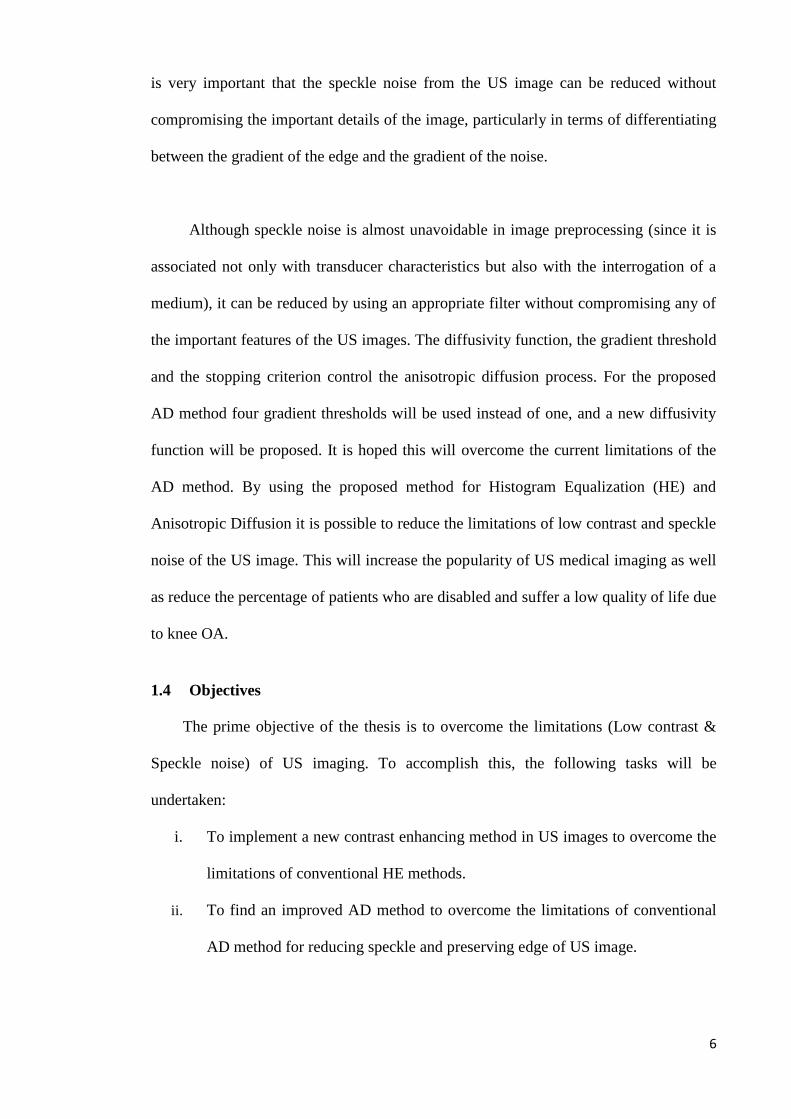
6
is very important that the speckle noise from the US image can be reduced without
compromising the important details of the image, particularly in terms of differentiating
between the gradient of the edge and the gradient of the noise.
Although speckle noise is almost unavoidable in image preprocessing (since it is
associated not only with transducer characteristics but also with the interrogation of a
medium), it can be reduced by using an appropriate filter without compromising any of
the important features of the US images. The diffusivity function, the gradient threshold
and the stopping criterion control the anisotropic diffusion process. For the proposed
AD method four gradient thresholds will be used instead of one, and a new diffusivity
function will be proposed. It is hoped this will overcome the current limitations of the
AD method. By using the proposed method for Histogram Equalization (HE) and
Anisotropic Diffusion it is possible to reduce the limitations of low contrast and speckle
noise of the US image. This will increase the popularity of US medical imaging as well
as reduce the percentage of patients who are disabled and suffer a low quality of life due
to knee OA.
1.4 Objectives
The prime objective of the thesis is to overcome the limitations (Low contrast &
Speckle noise) of US imaging. To accomplish this, the following tasks will be
undertaken:
i. To implement a new contrast enhancing method in US images to overcome the
limitations of conventional HE methods.
ii. To find an improved AD method to overcome the limitations of conventional
AD method for reducing speckle and preserving edge of US image.
7
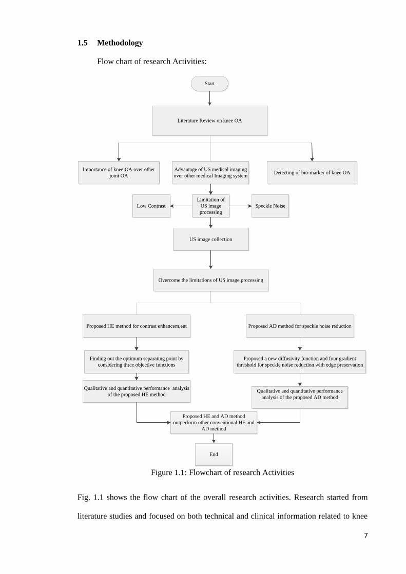
1.5 Methodology
Flow chart of research Activities:
Start
Literature Review on knee OA
Importance of knee OA over other
joint OA
Advantage of US medical imaging
over other medical Imaging systemDetecting of bio-marker of knee OA
Limitation of
US image
processing
US image collection
Overcome the limitations of US image processing
Proposed HE method for contrast enhancem,ent Proposed AD method for speckle noise reduction
Finding out the optimum separating point by
considering three objective functions
Proposed a new diffusivity function and four gradient
threshold for speckle noise reduction with edge preservation
Qualitative and quantitative performance analysis
of the proposed HE method Qualitative and quantitative performance
analysis of the proposed AD method
Proposed HE and AD method
outperform other conventional HE and
AD method
End
Low Contrast Speckle Noise
Figure 1.1: Flowchart of research Activities
Fig. 1.1 shows the flow chart of the overall research activities. Research started from
literature studies and focused on both technical and clinical information related to knee
8
OA detection. From the literature review, it became clear that knee OA is more common
than other human joint OA. Ultrasound imaging modality has been selected to
encounter the problem statement mentioned at section 1.3. Nevertheless, it has two
limitations include; low contrast ratio and speckle noise. For that reason, a novel
contrast enhanced and speckle noise reduction method has been proposed in this thesis.
A series of qualitative and quantitative analyses has been performed and we managed to
conclude that our proposed methods outperform other conventional HE and AD
methods.
1.6 Overview of each chapter
1.6.1 Chapter 1
Chapter 1 is the introduction of the thesis. This chapter discusses the necessity of knee
OA detection. Why is knee OA is more important than other joint OA? This chapter
explains the prevalence of knee OA in different countries. The problem statement of US
image for detecting knee OA also has been discussed in this chapter.
1.6.2 Chapter 2
Different medical imaging modalities including their advantages and disadvantages are
discussed in this chapter. The mechanism of US medical imaging has also been
described; which includes the limitations of US medical imaging, relations between
cartilage thickness and formation of knee OA, and biomarkers of knee OA. Technical
review of different conventional HE and AD system has been mentioned in this chapter.
Three controlling parameters of the AD method, namely the diffusivity function,
gradient threshold and stopping criterion and their importance are explained thoroughly.
1.6.3 Chapter 3
This chapter starts with the data acquisition for the research. The difference between
meniscus and cartilage in knee joints is clearly described in chapter 3. Construction of
three objective functions and obtaining a final equation from these three objective
9
functions for HE method has been proposed. Lastly, selected performance metrics for
the proposed HE and AD method are defined in this chapter.
1.6.4 Chapter 4
The qualitative analysis of the output image of cartilage and meniscus from different
HE and AD methods including our proposed method has been analyzed. In addition,
quantitative analysis by using numerical values of different performance metrics has
been explained. Last but not least, we have concluded the chapter with the precision of
the method using Fisher’s Least Significant Difference Test and Duncan Test.
1.6.5 Chapter 5
Conclusion and future work has been discussed in this chapter. The limitation of the
proposed HE and AD method has also been described in chapter 5.

10
CHAPTER 2 LITERATURE REVIEW
2.1 Background
A literature review has been carried on non-technical parts as well as technical
parts. A lot of research has already been conducted on image processing for improving
the quality of US images. Generally, US images suffer from two drawbacks; namely
low contrast ratio and speckle noise. For increasing the contrast of the US image
different Histogram Equalization (HE) methods have been used. A new HE method will
be proposed that will overcome the limitations of conventional HE methods. AD
filtering can also successfully remove the speckle noise, preserve the edge, small
structure and region boundary if its crucial parameters are scaled accurately. The
behavior of the AD filter is controlled by three parameters known as gradient
thresholds, conductance function and stooping criterion. By considering the first two of
these three parameters an improved AD method will also be proposed that will
overcome the limitations of the conventional AD method.
2.2 Different medical imaging systems
There are different types of imaging in medical imaging systems. Among them
are X-rays, Computed Tomography (CT), Magnetic Resonance Imaging (MRI) and
Ultrasound (US), which are the key diagnostic imaging tools used in modern health care
systems for studying illnesses.
2.2.1 Radiograph: X-Ray
Hillary et al (Hillary J. Braun a, 2012) mentioned that despite the vast
development of modern imaging modalities, radiography is still the most popular
medical imaging system in the evaluation of knee osteoarthritis. Generally, the
11
evaluation of knee joint is performed by using the extended-knee radiograph, which is a
bilateral anterior posterior image, It is acquired with weight-bearing patients having
both knee in full extension, Wilson et al (Wilson, 2009) has shown that X-ray imaging
has traditionally used film to capture the images. The formation of the images is
dependent on absorption of X-rays by structures of the body. The X-rays that are not
absorbed pass through the body and strike a film behind the area of the body. The light
and radiation sensitive film is sandwiched between two intensifying screens enclosed in
a light proof cassette. The screens convert the X-ray radiation into light, which acts in
the film. The film is then developed using chemicals, in the same way as for a
photograph. The film can then be placed on a light box to be viewed, and a diagnosis
made. Currently, flexed-knee radiographs having various degree of X-ray bean angle
and flexion have been used for improving intra articular visualization. For evaluating
joint space narrowing (JSN) and the formation of osteophyte radiographs are useful.
The grading schemes, namely the Kellgren-Lawrence grading scheme and the
established guidelines of Osteoarthritis Research Society International Classification
Score are popular for the diagnosis of knee osteoarthritis progression. A.J. Teichtahl, et
al. (A.J. Teichtahl, 2008) determined that JSN, a continuous measure, has been
employed as the outcome in studies of disease progression in knee osteoarthritis.
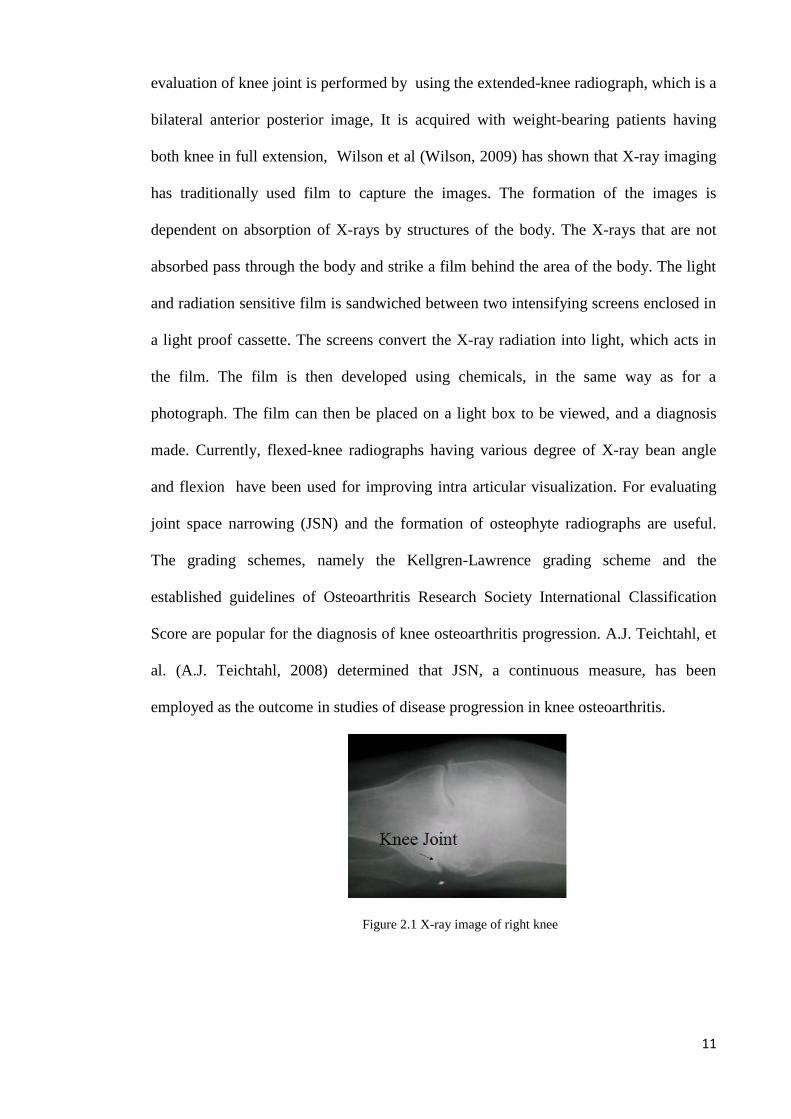
Figure 2.1 X-ray image of right knee

12
Fig 2.1(Source: http://en.wikipedia.org/wiki/Osteoarthritis’) shows the x-ray image of
right knee joint.
2.2.2 Computed Tomography (CT)
Computed Tomography (CT) uses cross-sectional images created multiple scans
in order to produce images of articular cartilage almost in real time. The endoscope is
placed at the cartilage at the time of endoscopy. It provides quantitative information on
the progression of disease, including information on structural changes in collagen as a
result of acute trauma or degenerative osteoarthritis. A computer assembles data from
the images to produce a resultant high resolution image in three dimensions.
Here tomos means "slice", and graphein means "write" (Evans, Godber, & Robinson,
1994). As it combines slices of images together to obtain the resultant image.
Figure 2.2 C.T. image of right knee
Fig2.2.(Source:https://www.radiology.wisc.edu/sections/msk/interventional/Knee_CT_a
rthrogram/index.php ) shows the C.T. image of right knee joint. The knee OA detection
of C.T. imaging has the same potentiality as the X-ray imaging as it generated from
several finely focused X-ray together.
2.2.3 Magnetic Resonance Imaging (MRI)
MRI is an imaging modality that produce images of structures and organ inside
the body by using pulse echo radio wave energy and a magnetic field. For imaging,

13
firstly the magnet of MRI scanner will create a magnetic field. The patients are then
passed through this magnetic field. The human body consists of 70% water. The
hydrogen atoms of water make up their individual magnetic field, this field is affected
by the stronger magnetic field created by the magnet of MRI scanner. This causes the
change of direction of the spin or magnetic moment of the atoms. This is then
accompanied by a radio frequency pulse which makes the spins align and spin at Larmour
Frequency. These data are collected by a computer and processed to create an MRI image.
Magnetic Resonance Imaging (MRI) imaging is very popular as it gives a very high
resolution image. According to (Hillary J. Braun a, 2012) image contrast is manipulated
by MRI to highlight different types of tissue. Common contrast methods include proton
density (PD), 2D or multi-slice T1-weighted and T2-weighted imaging. For evaluation
of focal cartilage defects, spin echoes and fast-spin echo (FSE) imaging techniques are
very useful. More recently, the use of turbo-spin or fast-echo imaging, water excitation
and fat saturation has seen enhanced contrast.
Scoring takes place through one of a number of existing systems, mostly
employing semi-quantitative and morphological measures. The modified outer bridge
scale is used for cartilage defect geometry, and whole-organ assessment is used to
assess cartilage articulation as a whole. This latter method has proved to be specific,
reliable, and able to monitor lesion progression. Amongst these, the Knee Osteoarthritis
Scoring System, the Boston Leeds Osteoarthritis Knee Score and Whole-organ
Magnetic Resonance Imaging (MRI) Score, are commonly used (Hunter et al., 2008).
Besides, L. Menasheyz et al (L. Menashe yz, 2012) has examined the performance of
MRI for diagnosis of knee OA. By using different parameters such as positive and
negative predictive values (PPV, NPV), specificity, positive and negative likelihood
value, sensitivity and accuracy MRI is able to differentiate between subjects having

14
knee OA or not. All the results gathered by using true negative (TN), true positive (TP),
false negative (FN) and false positive (FP) is termed as ‘overall sensitivity’ used for OA
detection. MRI is considered as the gold standard for knee OA detection. (Source:
http://www.physiopedia.com/Diagnostic_Imaging_of_the_Knee_for_Physical_Therapis
ts)
Figure 2.3 MRI image of right knee
Fig.2.3.(Source:http://blog.remakehealth.com/blog_Healthcare_Consumers0/bid/8031/
What-does-an-MRI-Scan-of-the-Knee-show) shows the MRI image of right knee joint.
The contrast ratio is high, not affected by speckle noise. The edge of tibia and femur are
easily detectable and the cartilage layers are very clear.
2.2.4 Ultrasound
A.J. Teichtahl et al (A.J. Teichtahl, 2008) stated that ultrasound is widely
employed to provide imaging guidance for procedures such as intra-articular injection
and biopsy for both the investigation and treatment of joint arthropathies. Thus, US is
helpful for detection of early osteoarthritis even without other clinical. Łukasz Paczesny
et al (Łukasz Paczesny, 2011) states “a reliable knee ultrasound examination requires
devices with modern software and high-frequency probes”. The probe frequency will
depend on the structure, but in general it will be between 7 and 10MHz, with the upper
end providing finer detail. Even higher frequencies, that is, approximately 13 MHz will
help to produce a “soft image” with high level of detail. This is because almost all
15
tissues around the knee that are examined by ultrasound are located superficially; the
need to use lower frequencies is limited to visualization of popliteal fossa and cruciate
ligaments. Besides, linear probe is a standard for musculoskeletal sonography and this
does not change in the knee. However, there are some specific situations, such as
visualization of the deeply located cysts in the popliteal region or posterior cruciate
ligament assessment, when convex, lower frequency probe (approximately 5 MHz) fits
better. Color Doppler and Power Doppler technique can be useful in complete knee
ultrasound diagnostics. It allows for the assessment of the vascularization of soft tissues
thus enhancing diagnostic possibilities in arthritis, tendinitis, tumors, and in the
monitoring of the healing processes. Henning Bliddal et al. (Hillary J. Braun a, 2012)
determined that the transducer frequencies of ultrasound systems higher than 12 MHz
produce sectional imaging with axial and lateral resolution which is less that 200 mm.
This allows ultrasound a perfect imaging modality to evaluate soft tissues surrounding
different joints. By using Doppler technique it is also possible to detect inflammatory
hyperemia as well as to quantify. Ultrasound is able to produce sound waves. These
sound waves are passed through the body, producing return echoes, these echoes are
collected by the transducer to produce visualize structure of body beneath the skin. The
ability of transducer to measure difference among the echoes reflected from various
tissues of the body allows an US image to be captured. The ultrasound technology is
especially suitable for observing accurate interference between fluid filled and solid
spaces. Unfortunately, the performance of ultrasound is not same for all joints. It differ
from one joint to another as well as one part of joint to another part. This causes as,
changes of depth of penetration will change the speed of ultrasound echo. For example,
the femoral articular cartilage of any kind can be investigated with ultrasound, whereas
it is almost impossible in case of tibial cartilage (Bliddal, Boesen, Christensen,
Kubassova, & Torp-Pedersen, 2008).
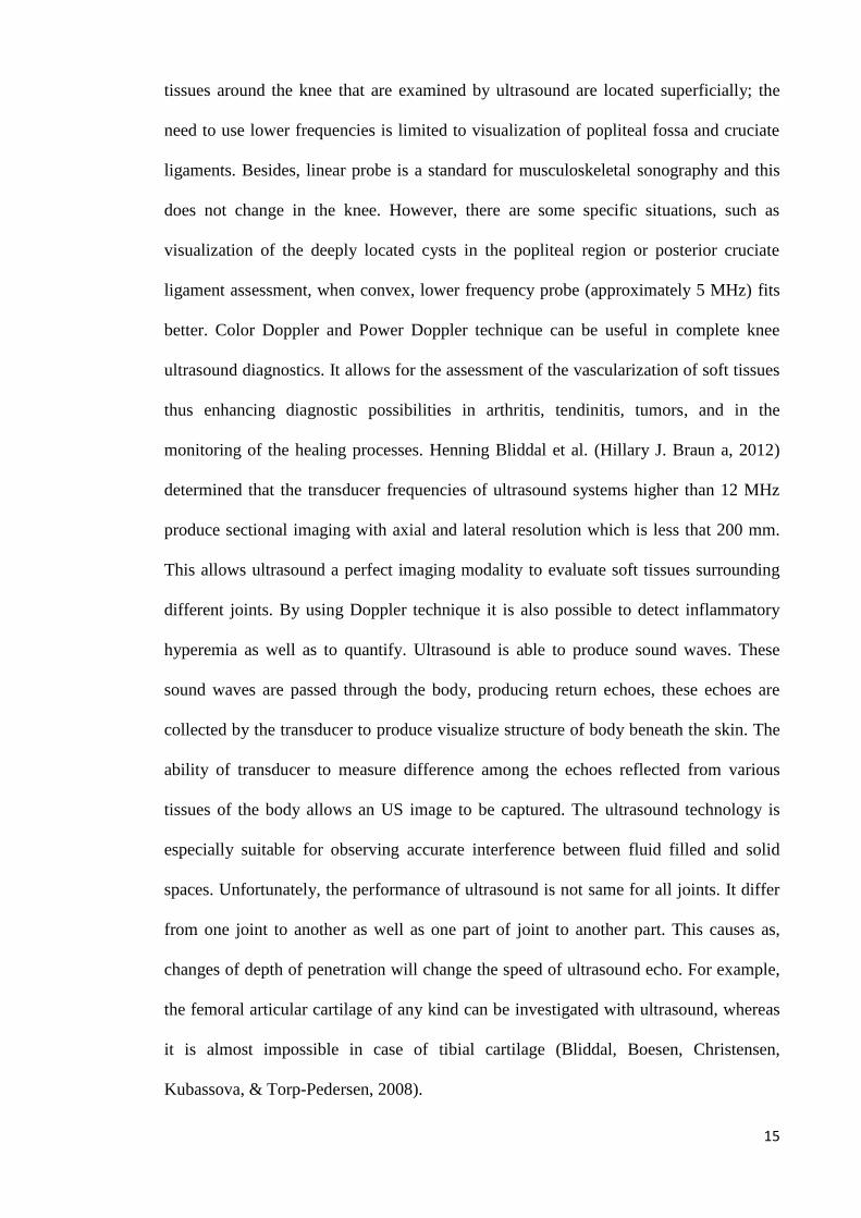
16
Figure 2.4 US image of right knee
Fig. 2.4 (Source: http://imaging.birjournals.org/content/14/3/188/F12.large.jpg) shows
the US image of right knee joint. It is highly affected by speckle noise. The edges are
fully undetectable.
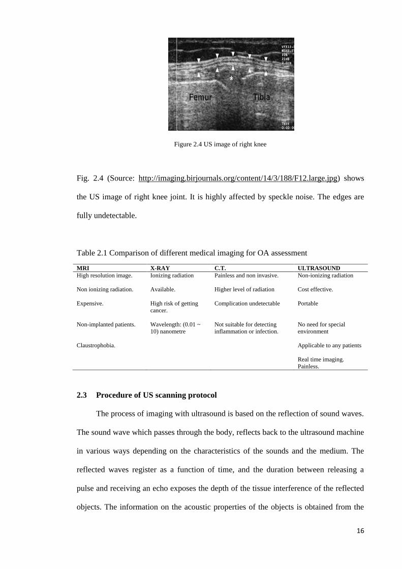
Table 2.1 Comparison of different medical imaging for OA assessment
MRI X-RAY C.T. ULTRASOUND
High resolution image. Ionizing radiation Painless and non invasive.
Non-ionizing radiation
Non ionizing radiation. Available.
Higher level of radiation Cost effective.
Expensive.
High risk of getting
cancer.
Complication undetectable Portable
Non-implanted patients.
Wavelength: (0.01 ~
10) nanometre
Not suitable for detecting
inflammation or infection.
No need for special
environment
Claustrophobia.
Applicable to any patients
Real time imaging.
Painless.
2.3 Procedure of US scanning protocol
The process of imaging with ultrasound is based on the reflection of sound waves.
The sound wave which passes through the body, reflects back to the ultrasound machine
in various ways depending on the characteristics of the sounds and the medium. The
reflected waves register as a function of time, and the duration between releasing a
pulse and receiving an echo exposes the depth of the tissue interference of the reflected
objects. The information on the acoustic properties of the objects is obtained from the

17
intensity of the echo objects. By using the received echo signal the US images are
constructed.(Source;http://www.physics.utoronto.ca/~jharlow/teaching/phy138_0708/le
c04/ultrasoundx.htm). To enhance the diagnostic utility of ultrasound images, contrast
agents have been developed. These contrast agents are injectable suspensions of gas
bodies that provide strong echoes from poorly echo genetic blood–filled regions as they
circulate in the blood. Contrast enhancement diagnostic ultrasound (CEDU) is described
in Douglas et al. (Douglas L. Miller, 2011) and has been used for the examination of,
kidney, Liver and other organs. The experiments by Scott et al. (Scott B. Raymond,
2008) showed the enhancement of ultrasound in case of the delivery of small
fluorescent agents and large biological immunotherapeutic for transgenic mouse models
carrying Alzheimer’s disease. It was also described by William et al. (William J. Tyler,
2008) that US has the ability to modulate neuronal activity . For accomplishing this
firstly it is needed the temporary suppression of spontaneous activity then US
transmission through the crayfish ventral nerve cords (Gavrilov LR, 1996). The
ultrasound guided method by Amanda et al. (Amanda Shanks Huynh, 2011) has
concluded that US is more suitable for examining the influence of immunotherapy on
tumor growth compare to the subcutaneous model. As US is a rapid imaging technique,
so by using ultrasound-guided HIFU it may possible to monitor real time tissue
responses (Tinghe Yu, 2011), as a result it decreases untoward lesions (G, 2007; JE,
2005). CT and MRI biopsies do not offer a real time image update but, based on
fundamental B-scan ultrasound image guided biopsies, it is possible to perform real
time image guided biopsies (Ernst Michael Jung, 2012).

18
Figure 2.5 Procedure of Image scanning by US machine
The steps of US image scanning are shown in Fig. 2.5. US images were taken from
different positions of the probe. The lateral side of the knee joint has been imaged
because by using this side, it was possible to better observation of the cartilage of the
knee joint. A 8MHz probe was used, as a high frequency probe can give a better
resolution of US image. With a high frequency, the wavelength will be smaller; smaller
imaging particles become detectable by using a higher frequency US probe. For the US
imaging of knee joint, notch was very important because the probe would be placed
beside the patella by using notch.
2.4 Problems with US medical imaging system
Though US imaging has a lot of advantages it suffers from two drawbacks,
namely speckle noise and low contrast ratio (O.Michailovich, 2006; P.M.Shankar,
2006). Low contrast is a major problem of US imaging. For enhancing contrast of the
US image, contrast enhancing gel is used. But still the contrast of the US image is very
poor. The low contrast of the US image is due to the mechanism of US imaging. It
depends upon the properties of the echo signal. Contrast of the US image can be
enhanced by using post processing in US images. Histogram Equalization (HE) is very

19
popular for contrast enhancement of the US images as it is very simple and effective.
However, the conventional HE method has some limitations. In this thesis a novel
contrast enhancement method will be used that will overcome the limitations of the
conventional contrast enhancing method.
Speckles occur in US images when a non-coherent detector and a coherent source are
used to interrogate a medium having a rough surface on the scale of the typical
ultrasound wavelength. US speckle noise generally occurs in soft organs such as the
liver or kidney, as the underlying structure of these organs is very small compared to the
large wavelength (L.C.Gupta, 1998) of ultrasound. Speckle noise generally consists of a
high gray level of intensity which qualitatively ranges from hyperechoic (bright) to
hypoechoic (dark) domains. They are more granular at low frequency than at a high
frequency. There are many factors associated with speckle noise, including the phase
sensitivity of a transducer, the number of scattered beams, and their coalition, the
distance between objects and the transducer, and the transducer frequency (D. Adam,
2006). The consequence of speckle noise (A.K.Jain, 1989) is a poor image quality,
including ruined spatial and contrast resolution. It also reduces the signal to noise ratio
(SNR), the peak signal to noise ratio (PSNR), the structure similarity index
measurement (SSIM), the edge preservation index, and increases the mean square error
(MSE). However, speckle sometimes holds some useful information in US images,
which is obscured due to the low resolution and contrast. Therefore it is highly desirable
to reduce speckle noise without compromising any of the important features of the US
images (C.B.Burckhardt, 1987; F.Zhang, 2007b).
There are two basic techniques for reducing speckle noise (Navalgund Rao, 2002) from
ultrasound images: a) compounding approach, and b) post-processing approach (Adam,
2006). The compounding approach involves modifying data acquisition by generating a
20
single image from a number of images focused in the same region (Behar, 2003;
Jespersen, 1998; Stetson, 1997; Trahey, 1986). On the other hand, the post-processing
approaches include a variety of filtering techniques for image processing to reduce
speckle from US images. The compounding approach is much more expensive
compared to the post-processing approaches. Filtering techniques are post-processing
approaches which will be mainly discussed in our thesis. Filtering techniques have
proven to be useful for reducing unwanted speckle and enhancing image quality. There
are two basic types of filtering techniques available in the literature, namely linear
filtering and nonlinear filtering.
Linear filtering approaches (A. Lopes, 1990; D.T. Kuan, 1987; J. S. Lee, 1986; X. Hao,
1999) applied in early speckle suppression systems. However, linear methods had some
limitations such as suppression being accomplished at the cost of significant smoothing
of structural details, and a lack of balance between edge preservation and noise
reduction. Non-linear filtering methods were found to be more successful as they were
able to overcome the limitations of linear filters. A number of research studies have
investigated the improvement of the nonlinear filtering approach. The improvement of
the US image filtering method for speckle reduction is a continuous process. Different
techniques (multi look method, spatial averaging, and homomorphic filtering) are being
used for suppressing the speckle of US images. Among them, the AD method is the
most popular method for suppressing the speckle of the US image (Ovireddy &
Muthusamy, 2014). However, it suffers from some drawbacks such as having to make a
compromise between speckle noise reduction and edge preservation during noise
suppression. In this thesis, a new anisotropic diffusion (AD) method will be proposed
by considering its three parameters known as the diffusivity function, gradient threshold

21
and stopping criterion, which together control the efficiency of the AD method. The
proposed method will overcome the limitations of the conventional AD method.
2.5 Relationship between cartilage thickness and formation of OA
Cartilage loss is the main feature of the knee OA. By using MRI it is possible to
directly visualize the articular hyaline cartilage. Assessments of cartilage morphology
from knee MRI are emerging as promising measures for monitoring OA disease
progression (Eckstein F, 2006). Knee alignment is also associated with the progression
of knee OA. By using joint space narrowing it is also possible to determine the stage of
knee OA. But this is not possible due to cartilage quantification being as yet imprecise
through medical imaging. By using medical imaging systems, it is however possible to
detect a small change of the cartilage of the knee joint, if image processing is
accomplished on the captured US images. A few investigators have reported that 4-8%
of cartilage loss occur due to OA progression in each year(Eckstein F, 2006).
2.6 Biomarkers of knee OA
To diagnosis knee OA radiographs are very helpful. The OA affected knee joints
are characterized as follows. (1) With the progression of knee OA, cartilage will be
wear away, as a result joint space between knee bones will be narrower. (2) Since
cartilage will be destructed, the body will attempt to repair the knee joint, therefore
fluid-filled cavities or cysts will be formed. (3) Due to knee OA progression, cartilage
will be reduced, therefore knee bone will rub against each other, consequently creating
friction and uneven joints. (L.J. Bremner JM, Miall WE, 1968).
2.7 Benefits of US medical imaging over other medical imaging system
X-ray and CT are involved with ionized radiation and MRI is contra-indicated for
patients with metallic implants and patients having claustrophobia. C.T. exposes the
22
patient to higher levels of radiation and is limited to the detection of complications such
as fracture. Though MRI gives high resolution images it is costly and time consuming.
On the other hand, US is free from these limitations. US is a very popular diagnostic
tool capable of accessing patients without any restrictions, being painless, low cost,
non-invasive, and portable (A.Bezerianos A.Achim, 2001; B.Sahiner, 2007; J.Shan
H.D.Cheng, W.Ju,Y.Guo,L.Zhang, 2010). Most importantly, it provides real time
imaging which is not possible by using most other medical imaging systems. V.P.
Subramanyam Rallabandi et al (Rallabandi, 2008) mentioned that in the case of CT and
MRI, it is required to inject a blood pool contrast agent, which gives less spatial image
resolution and it has a low volumetric imaging speed for laymen visualization of large
vessels, a limitation on the utility of CT and MRI. US is easy to operate. Its potentiality
is high, for example, its resolution is as high as MRI for soft tissue (T. Marshburn,
2004; V. Noble, 2003). High frequency sound ranges from 20 kHz up to the several
GHz used in US imaging (K., 2002). In case of remote areas MRI, CT and X-ray
facilities are almost impossible. In these areas only US medical imaging system can be
easily provided for diagnosis, because US probes are portable and easy to carry.
For the above mentioned reasons the use of US is growing at least at a rate of 8% per
year. On 2009-10, 34.4% of the total diagnostic imaging methods used were ultrasound-
based. In the financial year of 2005-06 the total service by the ultrasound images was
4,716,304, and in 2009-2010 it was 6,251,413. (Source: Date of processing Medicare
data, Australia) ("Medical Benefits Reviews Task Group Diagnostic Imaging Review
Team Department of Health and Ageing February 2012 Review, Australia,"). In
Malaysia, ultrasound machines have been widely used in hospitals. They are used for
imaging of the uterus, ovaries, pelvic organs, and for the presence of a foetus via the

23
abdomen. Recently, ultrasound machines are becoming popular for the imaging of joints
such as knees or hips. From National Medical Device Statistics of 2009, US machines
are widely available in the country, with the higher numbers in the public (62.7%) rather
than in the private sector (37.3%). Overall, Selangor and Putrajaya reported the highest
number of ultrasonography systems (USG) (130), followed by Johor (74) and Kedah
(60), in contrast to Perlis, Melaka and Terengganu which recorded 7, 9 and 18 devices
respectively. From these statistics, it appears that the application of US procedures has
been positively received by Malaysia. New developments and research into US
applications will possibly increase these statistics further.
2.8 Technical Review of HE and AD method
In case of contrast enhancement, (HE) is very popular as it is very simple and
effective. But conventional HE has some limitations, such as there being a mean shift of
the output image. The brightness preservation and detail preservation does not occur at
the same time during the contrast enhancement. Either brightness or detail preservation
occur during contrast enhancement. So the aim of our proposed method will be to
preserve brightness and details during the contrast enhancement of the US image.
On the other hand, in case of a conventional AD method, its effectiveness depends on
the ability of the diffusivity function that will differentiate between the gradient of edge
and gradient of noise, the gradient threshold parameters and diffusion stopping criterion.
So for improving the efficiency of the proposed AD method a new diffusivity function
as well as four gradient thresholds instead of one will be considered for effective edge
preservation and successful noise reduction.
2.8.1 Review of existing contrast enhancement system
The conventional HE (Lau, 1994) method is described as follows:

24
If the input image is 𝑋(𝑖, 𝑗), total number of pixels are n in the gray scale level ranges
from [𝑥0 − 𝑥𝑁−1]. Then the probability density function 𝑃𝑟𝑙 for level of 𝑟𝑙 is defined as
𝑃𝑟𝑙 =𝑛𝑙
𝑛 (2.1)
Here, n represents the total number of pixels in the image and 𝑛𝑙 is the frequency of the
occurrence of the level 𝑟𝑙 in the input image and 𝑙 = 0,1, … … , 𝑁 − 1. The histogram of
the image is defined as plot of 𝑛𝑙 against 𝑟𝑙. The cumulative density function is given by
𝐶(𝑟𝑙) = ∑ 𝑃𝑟𝑖𝑙𝑖=0 (2.2)
Histogram Equalization is then used to map the image into the entire dynamic range
[𝑋0 − 𝑋𝑁−1]. It is done by using the cumulative density function, shown as the
following equation
𝑓(𝑋) = 𝑋0 + (𝑋𝑁−1 − 𝑋0) ∗ 𝐶(𝑟𝑙) (2.3)
which flattens the histogram of an image and causes a significant change in the
brightness.
The equation of the output image of the HE is 𝑌 = {𝑌(𝑖, 𝑗)}, which can be expressed as
𝑌 = 𝑓(𝑥) = {𝑓𝑋(𝑖, 𝑗) |∀𝑋(𝑖, 𝑗) ∈ 𝑋} (2.4)
A new brightness preservation method based on HE, named Brightness Preserving Bi-
Histogram Equalization (BBHE), was proposed by Kim (Kim:, 1997). Based on the
threshold of separation of the input histogram, different types of bi-histogram
equalization methods can be proposed. The input image X can be decomposed into two
sub-images, 𝑋𝐿and 𝑋𝑈, based on the threshold of separation. If 𝑋𝑇 is the threshold of
separation then 𝑋𝑇 ∈ {𝑋0𝑋1 … … . 𝑋𝑁−1}. From this, the following can be obtained:
𝑋 = 𝑋𝐿 ∪ 𝑋𝑈 (2.5)
where
𝑋𝐿 = {𝑋(𝑖, 𝑗)|𝑋(𝑖, 𝑗) ≤ 𝑋𝑇 , ∀𝑋(𝑖, 𝑗) ∈ 𝑋}
and
𝑋𝑈 = {𝑋(𝑖, 𝑗)|𝑋(𝑖, 𝑗) > 𝑋𝑇 , ∀𝑋(𝑖, 𝑗) ∈ 𝑋}

25
Thus the PDF of the sub-image 𝑋𝐿 and 𝑋𝑈can be written as
𝑃𝐿(𝑋𝐾) =𝑛𝑘
𝑛𝐿 , 𝑘 = 0,1, … … … 𝑇 (2.6)
and
𝑃𝑈(𝑋𝐾) =𝑛𝑘
𝑛𝑈 , 𝑘 = 𝑇 + 1, 𝑇 + 2, … … 𝐿 − 1 (2.7)
where the number of 𝑋𝐾 in 𝑋𝐿 and 𝑋𝑈 is represented by 𝑛𝑘 . 𝑛𝐿 is the total number of
sample in 𝑋𝐿, and 𝑛𝑈 is the total number of sample in 𝑋𝑈.Thus, the cumulative density
functions of 𝑋𝐿 and 𝑋𝑈 are defined as
𝐶𝐿(𝑋𝐾) = ∑ 𝑝𝐿𝑇𝑘=0 (𝑋𝐾) (2.8)
and
𝐶𝑈(𝑋𝐾) = ∑ 𝑝𝑈𝐿−1𝑘=𝑇+1 (𝑋𝐾) (2.9)
In HE, the cumulative density function acts as a transform function. Like HE, the
cumulative density function of each sub-images is
𝑓𝐿(𝑋𝑘) = 𝑋0 + (𝑋𝑇 − 𝑋0)𝐶𝐿(𝑋𝐾), 𝑘 = 0,1, … … … . , 𝑇 (2.10)
and
𝑓𝑈(𝑋𝑘) = 𝑋𝑇+1 + (𝑋𝐿−1 − 𝑋𝑇+1)𝐶𝑈(𝑋𝐾), 𝑘 = 𝑇 + 1, … … … … … , 𝐿 − 1 (2.11)
In BBHE, the threshold of the separating point (𝑋𝑇) is the mean brightness of the input
image. By using this process, it is possible to preserve the image original brightness
which is not possible if using conventional HE.
DSIHE (Dualistic sub-image histogram equalization) has been proposed by Wan et
al.(Yu W, 1999), which is the extension of BBHE. It functions by selecting the
threshold separating point at the median of the histogram. DSIHE has been proven able
to outperform BBHE in terms of brightness preservation and entropy. However, both
BBHE and DSIHE may fail to enhance and preserve their original brightness under
certain conditions. MMBEBHE (Minimum mean brightness error bio-histogram
26
equalization) was proposed by Chen and Ramli (Soong-Der C, 2003b), which is the
extension of BBHE, in which the yield minimum difference between input and output
mean is known as Absolute Mean Brightness Error (AMBE). However, this method is
also not free from undesirable effects. After that, Chen and Ramli proposed RMSHE
(Recursive Mean Separate Histogram Equalization) (Soong-Der C, 2003a). It functions
by recursively making partitions of the given image histogram. Each segment is
equalized independently and the contrast enhanced output image is achieved by the
union of all the segments. A similar method, named Recursive sub-image histogram
equalization (RSIHE), was proposed by Sim et al. (Sim KS, 2007). The difference
between RMSHE and RSIHE is that, in the case of RMSHE, the mean is used as the
separating point, whereas median is used as the separating point in case of RSIHE.
Next, Weighted Thresholded HE (WTHE) (Wang Q, 2007) was also proposed. It can
control the enhancement process by using an adaptive mechanism. It has two merits;
viz. ease of control and ability to adapt to different images. There are also two more
weighing techniques; are Recursive Separated and Weighted Histogram Equalization
(RSWHE) (Kim M, 2008) and Weight Clustering Histogram Equalization (WCHE)
(HK., 2008). SRHE (NSP, 2009) (Sub Region Histogram Equalization) was proposed
by Ibrahim and Kong. In this method, a Gaussian filter is used for partitioning the input
image. Recently, Zuo et al proposed RLBHE (Range Limited Bi-Histogram
Equalization) (Zuo Chao, 2012). A threshold which can minimize the intra class
variance is used as the separating point for RLBHE. However, the above mentioned
methods only consider one of the characteristics of the image while neglecting the
others. For example, BBHE, MMBEBHE, RMSHE and RSIHE only consider on
brightness preservation and pay less attention on detail preservation. On the other hand,
the clipping methods of ‘Kim et al.’ and ‘Seungjoon et al.’ (Kim T, 2008; Seungjoon Y,

27
2003) only focus on detail preservation while neglecting the importance of brightness
preservation.
The aim of the thesis is to propose a HE method which can preserve the brightness and
detail while enhancing the contrast of the image, which can be done by using the
Multipurpose Beta Optimized Recursive Bi-Histogram Equalization (MBORBHE)
method. For this reason three objective functions named Preservation of Brightness
Score function (PBS), Optimum Contrast Score function (OCS) and Preservation of
Detail Score function (PDS) will be considered. By using these three objective functions
we will find the optimum separating point for segmenting the histogram of the input
image. This method improves the traditional method used in HE, where histogram
equalization emphasizes only one criterion but ignores the others. The motivation of this
work is to produce a more comprehensive and natural output image by taking all
properties into account.
2.8.2 Review on existing speckle reduction methods
A suitable method of speckle reduction is one which enhances the value of
signal to noise ratio while preserving the lines and edges of the image. Gaussian noise is
an additive noise, whereas speckle noise is in multiplicative form (Tur, Chin, &
Goodman, 1982).
𝑣 = 𝑢. 𝑛 (2.12)
Where u denote the image to be recovered. v is the corrupted image and n is the speckle
noise. The recovery of speckle noise is much harder than the recovery of conventional
Gaussian additive noise. The reason of this is that speckle noise is signal correlated as
well as its distribution being much more complicated compared with additive Gaussian
noise.
28
Temporal averaging (Fuk-kwok, 1983) is the first widely used speckle reduction method
for US images. This method is based on averaging multiple uncorrelated frames of the
same scene to prevent the speckle effect. Though this method was very simple and fast,
it produced blurry images and detail was lost. To overcome this, Loupas et al (Loupas,
McDicken, & Allan, 1989) proposed a speckle reduction filter which was named the
adaptive weighted median filter (AWMF). In this method weight median is used for
suppressing the speckle noise. By using local statistics for each pixel smoothing
characteristic and weight coefficient is adjusted. After that, the adaptive speckle
suppression filter (ASSF) was proposed by Karaman et al(Karaman, Kutay, & Bozdagi,
1995). It was also based on the local statistics of the pixel. By using appropriate size and
shape of the local filtering kernels filter adaptation was achieved. After that Czerwinski
et al.(Czerwinski, Jones, & O'Brien, 1999) proposed a ‘stick’ method which will detect
the tissue boundaries and suppress speckle noise. On the other hand another group of
researcher has proposed some other speckle reduction filters such as Box filter (F.-K.
Li, Croft, & Held, 1983), Median filter, Lee filter (J.-S. Lee, 1980), Frost filter(Frost,
Stiles, Shanmugan, & Holtzman, 1982) and Kuan filter (Kuan, Sawchuk, Strand, &
Chavel, 1987).
A box filter is a conventional Low pass filter. It can smooth the details (such as edge
and point) and remove the noise of high frequency spectrum. It is a simple average
filter. A median filter is effective for speckle reduction. The use of median intensity of a
properly shaped and sized filtering window which surrounds the central pixel acts as the
output of the target pixel. It can successfully reduce noises whose size is less than half
of the filtering window. As filtering window size determines the rate of smoothing in
case of median filter, it sometimes removes some high frequency signals which lead to

29
blurring the edge of the image. This filter also undermines the effectiveness of
despeckling as it does not consider the statistical characteristic of speckle.
In the case of Lee filter, for filtering multiplicative noise, additive noise and the mix of
the two, it uses minimum mean square error (MMSE) for designing. By a weighted
average based on the variance and mean of sub-region, its output is estimated. In the
case of the frost filtering method it is designed by using an exponentially damped
convolution kernel adapted to image fine details. Based on the local statistics its output
is calculated. Lee and frost filter are also called statistical adaptive filters as they take
into account the statistical characteristics of speckle. The Kuan filter is similar to the
Lee filter but its weighting function is different from the Lee filter. The performance of
these filters is better but they have to compromise between smoothing in homogeneous
regions and preserving edges or sharp features of the original image.
The Non Local Mean (NLM) filter (Buades, Coll, & Morel, 2005) uses a high degree of
redundancy in the original image for denoising. It is a weighted Gaussian filter. As it
uses region comparison, it performs better in sharp edge preservation and Gaussian
noise suppression. But it does not show good result in the case of US imaging as
speckle in US imaging is subject to Rayleigh distribution.
Perona-Malik proposed a new definition of scale-space through Anisotropic Diffusion
(AD) (P. Perona, 1990) which is based on a non-linear partial differential equation
based diffusion process. It has recovered the demerits of linear smoothing, for example,
blurring the edge and eliminating important detail during speckle noise reducing
process. After that Yu and Acton (Y. Yu, Acton, S.T., 2002) used statistical method to
analyze speckle suppression and proposed Speckle Reducing Anisotropic Diffusion

30
(SRAD). It is space-variant and nonlinear filter. This method reduces speckle by
applying isotropic diffusion in homogeneous region and preserves edges by stopping
diffusion across the edges. This obtains a balance between speckle reducing and edge
preserving. Though this method is better, sometimes the SRAD based method generates
visually disappointing output when they are applied to filter primary noise contained in
US images, which is assumed to be Gaussian distribution. After that Zhang et al (Zhang,
2007) proposed LPND (Laplacian pyramid nonlinear diffusion). This method is able to
control the diffusion process more precisely and give the better result compare to SRAD
method. In this method to decompose the image into different sub-band Laplacian
pyramid has been utilized as a multi-scale analysis tool. After that, for suppressing noise
from each sub-band, anisotropic diffusion with different diffusion flux has been used.
But this method has also some limitations such as it is sensitive to several key
parameters. Due to the adopted model of the speckle, this approach was not very robust.
For the speckle reduction of optical coherence tomography image, Gilboa et al.
(G.Gilboa, 2004) proposed nonlinear complex diffusion (NCD) method. It combines the
property of both forward and reverse diffusion and removes the limitations of
conventional Peroma-Malik model. The Perona-Malik model has a lot of practical and
theoretical demerits. Catte et al.(F.Catte´ 1992) has proved that the diffusivity functions
of Perona-Malik are ill posed. In the case of noisy images the gradient generated by the
image features is comparable to the gradient generated by the noise. As a result in this
case, the conditional smoothing does not reduce the noise effectively rather than in case
of some images it enhances the noise. It has also no contribution in preserving the edge
as gradient of image are comparable to the gradient of noise. AD filtering can
successfully smooth the noise and preserve the edge along with small structures and
region boundaries if its crucial parameters are scaled accurately. The behavior of the
AD filter is controlled by three parameters known as gradient threshold perimeters,

31
diffusivity function and stooping criterion. If the gradient threshold is overestimated
then the resultant image will be over smoothed. On the other hand, its noise reduction
ability will degrade due to underestimation of the gradient threshold. Therefore,
selecting suitable gradient thresholds is very important for getting better resultant
images. In AD several conductance functions can be used, and different conductance
functions will differentiate the filtering results, which is shown in Black et al. (Black,
Sapiro, Marimont, & Heeger, 1998). For improving the performance of the AD method
it is important to choose an appropriate conductance function and scale it in such a way
so that it preserves the edge efficiently. It is also necessary for the gradient threshold
parameter will be decreasing function of time, which is depicted in (X. Li & Chen,
1994). In this way, it can preserve edge above a certain decreasing threshold. Our
method has been proposed by considering the gradient threshold parameters and the
diffusivity function.
There are wide range of applications of anisotropic diffusion (Gerig, Kubler, Kikinis, &
Jolesz, 1992; K.Z.Abd-Elmoniem, 2002; Krissian & Aja-Fernández, 2009; Krissian,
Westin, Kikinis, & Vosburgh, 2007; Mittal, Kumar, Saxena, Khandelwal, & Kalra,
2010) in the field of biomedical imaging. The goal of our thesis is to make the optimum
choice and scale of the diffusivity function of the AD method to get a better quality of
output image. Estimating the gradient threshold parameters is also considered for
effective noise reduction and edge preservation of the US image.
2.8.3 Anisotropic diffusion (AD) model
Perona and Malik (P.Perona, 1990) first proposed the following non-linear
diffusion model for speckle reduction or smoothing image in the continuous domain.

32
{𝜕𝐼
𝜕𝑡= 𝑑𝑖𝑣[𝑔(|∇𝐼|). ∇𝐼]
𝐼(𝑡 = 0) = 𝐼0
(2.13)
Here div is the divergence operator. 𝛁 is the gradient operator. ∥ indicate the magnitude,
𝑔(|∇𝐼|) is the diffusion coefficient or edge stopping function. I0 is the original image.
Anisotropic diffusion method will reduce the noise of the original image and make the
image smoother. Diffusion is encouraged in the homogeneous region and discouraged
across boundaries with step gradients. Perona and Malik suggested two diffusivity
function.
𝑔(|∇𝐼|) =1
1+(|∇𝐼|/𝑘)2 (2.14)
and
𝑔(|∇𝐼|) = exp [−(|∇𝐼|/𝑘)2] (2.15)
Where the edge magnitude parameter is denoted by k. It has a vital role to differentiate
the gradients generated by edges and those by noise.
In the case of the anisotropic diffusion method, the gradient magnitude |∇𝐼| is used as
the edge detector. It is used to detect an image boundary or edge as a step discontinuity.
When |∇𝐼| >>k, than 𝑔(|∇𝐼|) → 0 it will be all pass filter and diffusion flux is
suppressed and when |∇𝐼| <<k, then 𝑔(|∇𝐼|) → 1, it will be Gaussian filtering and the
diffusion flux will be encouraged. In fact k serve as a threshold for the diffusion process
if the value of k is larger, smoother homogenous region will be produced and vice versa.
The discretization form of Perona and Malik model is as follow
𝐼𝑡+1(𝑠) = 𝐼𝑡(𝑠) +𝜆
|𝜂𝑠|∑ 𝑔𝑘(|∇𝐼𝑠,𝑝|)∇𝐼𝑠,𝑝𝑝𝜖𝜂𝑠
(2.16)
Here, discretely sampled image is denoted by It, pixel position in the discrete 2-D grid is
indicated by s, the iteration steps are t. k is the gradient threshold parameter and g is the
conductance function. 𝜆𝜖(0,1) controls the rate of diffusion, 𝜂𝑠 represent the spatial 4-
pixel neighbourhood of pixel s. Here 𝜂𝑠 = {𝑁, 𝑆, 𝐸, 𝑊} where N,S,E and W are North,

33
South, East and West neighborhood of pixel s, respectively. As a result |𝜂𝑠| is equal to
4. The symbol ∇ denotes the gradient operator of continuous form. It also represent a
scalar defined as the difference between the center and neighboring pixel of each
direction.
∇𝐼𝑠,𝑝 = 𝐼𝑡(𝑝) − 𝐼𝑡(𝑠), 𝑝𝜖𝜂𝑠 = {𝑁, 𝑆, 𝐸, 𝑊} (2.17)
Though Perona and Malik’s model is very popular, it suffers from two practical and
theoretical drawbacks. The first one is very obvious and every researcher will raise
questions about it. If the signal is noisy with white noise then it will introduce very
large, unbounded oscillation of gradient ∇𝐼 . In this case the conditional smoothing
proposed by the model will not work as these noise edges will be untouched. However,
Perona and Malik’s model also proposed to include some low pass filters for smoothing
the image before applying the diffusion equation. The drawback of this is introducing a
new parameter in the method (low pass filter). On the other hand it seems to adopt again
what it tried to avoid, introducing a non-adaptive filter which causes the loss of the edge
preservation(Black et al., 1998).
The second drawback arises from the diffusivity functions type of 𝑔(𝑝) = 𝑒−𝑝 or
𝑔(𝑝) = (1 + 𝑝2)−1. For these functions, no correct theory of (2.13) is available. For
obtaining both uniqueness and existence of the conductance function g, it has to be
verified so that pg(p) is non-decreasing. If it is not non-decreasing then the process will
become unstable. Now the reason that the Perona-Malik model is unsuitable if pg(p) is
non-increasing will be explored. Firstly it will be considered in case of one-dimensional
signal. In that case the Perona Malik equation will be
𝑑𝐼
𝑑𝑡− (𝑔(𝐼′)𝐼′)′ = 0 (2.18)
Which can be written as 𝑑𝐼
𝑑𝑡− (𝑔′(𝐼′)𝐼′ + 𝑔(𝐼′))𝐼′′ = 0 (2.19)

34
If at some point p, pg(p) is decreasing with a negative derivative –a at p, that will cause
I'(x) =p, at some point x. Then the equation near x will look like 𝑑𝐼
𝑑𝑡+ 𝑎𝐼′′ = 0 . Which
is known as the inverse heat equation. It is an ill-posed equation for image processing as
the inverting of this equation is a perfect de-blurring algorithm (Osher & Rudin, 1990).
To overcome these two drawbacks Catte et al. (F.Catte´ 1992) has proposed the
following diffusion equation. Which is the modification of Perona-Malik model and
known as Catte_PM diffusion model (J. Yu, Tan, & Wang, 2010).
{𝜕𝐼
𝜕𝑡= 𝑑𝑖𝑣[𝑔(|∇(𝐺(𝜎) ∗ 𝐼)|)]
𝐼(𝑡 = 0) = 𝐼0
(2.20)
where
G(σ)= Gaussian kernel function and σ is the standard deviation. * denotes the
convolution and G(σ)*I denotes a convolution of the image at time t with Gaussian
kernel. By using this equation Catte_PM model became noise insensitive to the noises
whose scale smaller than σ. By this way the probability of noise misinterpreted near the
edge is vastly reduced. The diffusivity of the Catte_PM is computed as follows
𝑔(|∇𝐼|) =1
1+(|∇(𝐺(𝜎)∗𝐼)|
𝑘)
2 (2.21)
𝑔(|∇𝐼|) = exp [−(|∇(𝐺(𝜎) ∗ 𝐼)|/𝑘)2] (2.22)
For our proposed method Catte_PM model of (2.20) will be used as it will efficiently
denoise the image having high level of noise and overcome the above mentioned
demerits. In this case to automatically determine the value of σ relating to the Gaussian
noise of the image, a window size from 20⤬20 and 65⤬65 pixel is considered. It is done
for the satisfactory statistical calculation. By using this window size the most uniform
block of pixel in the image is determined. The pixels standard deviation of each block is
calculated. Finally the standard deviation of the most uniform block will be used as the
35
σ of the Gaussian filter. The smoothing Gaussian filter size is determined by using the
value of σ as described in (Petrou & Petrou, 2010).
The effectiveness of the AD method depends upon three factors; viz the ability to
differentiate between the gradient of edge and the gradient of the noise, the preciseness
of edge stooping function from preventing edge being smoothed, and the determination
of termination time of diffusion process automatically (J. Yu, Wang, & Shen, 2008). It
is known that noise in US images is multiplicative in nature, which means that the
variance caused by noise may be equal or larger than the variance caused by the edge.
For that reason to design an edge detection method that will separate noises from the
edge during conducting the diffusion process is not an easy task. Because of this the
conventional AD method proposed by Perona-Malik is ineffective in case of US image
despeckling. Therefore, the aim of this thesis is to propose an AD method that will give
emphasis on effective edge detection during speckle reduction. For that reason it will be
required firstly to obtain knowledge about diffusivity/conductance functions, Gradient
thresholds, and stopping criteria of the AD method. Then these parameters for the
proposed method will be defined.
2.8.3.1 Diffusivity function
In the AD method several diffusivity functions can be used, although different
diffusivity functions will differentiate the filtering results, which is shown in Black et al.
(Black et al., 1998). So, for improving the performance of the AD method it, is
important to choose an appropriate diffusivity function and scale it in such a way so that
it preserves the edge efficiently. In the case of the Perona Malik model, the first
diffusivity function (2.14) gives an emphasis on a wide region over a smaller one. On
the other hand, the second diffusivity function (2.15) puts emphasis on high contrast

36
edge over low contrast edge. Another diffusivity function has been proposed by Black et
al. (Black et al., 1998) which generates a sharper edge, showing better experimental
results of noise reduction, as the diffusion process converges fast. The diffusivity
function proposed by Black et al is as follows:
𝑔3(𝑥) = {1
2[1 − (
𝑥
𝑠)
2
]2
, 𝑥 ≤ 𝑠
0 𝑜𝑡ℎ𝑒𝑟𝑤𝑖𝑠𝑒
(2.23)
Where, 𝑆 = 𝑘√2 and 𝑥 = ∇𝐼
The flow function is defined as follows
𝜑(𝑥) = 𝑔(𝑥)𝑥 (2.24)
Where 𝜑(𝑥) represents the total generated brightness flow. At a location where x=k,
maximum flow will occur. For understanding the behavior of different diffusivity
functions, we will give emphasis on the scaling as well as comparison done by Black et
al.(Black et al., 1998) For comparing the efficiency, Black et al. has scaled the
diffusivity functions g1, g2 and g3 in such a way, so that their flow functions reach the
same maximum value, and that means an equal amount of brightness at the same point
x=0.2 shown in Fig.2.1 Which makes the modified version of following g1, g2 and g3.
𝑔1(𝑥) = exp [− (𝑥
𝑘√2)
2
] (2.25)
𝑔2(𝑥) =1
1+(𝑥
𝑘)
2 (2.26)
𝑔3(𝑥) = {0.67 [1 − (𝑥
𝑘√5)
2
]2
0 𝑜𝑡ℎ𝑒𝑟𝑤𝑖𝑠𝑒
𝑥 ≤ 𝑘√5 (2.27)
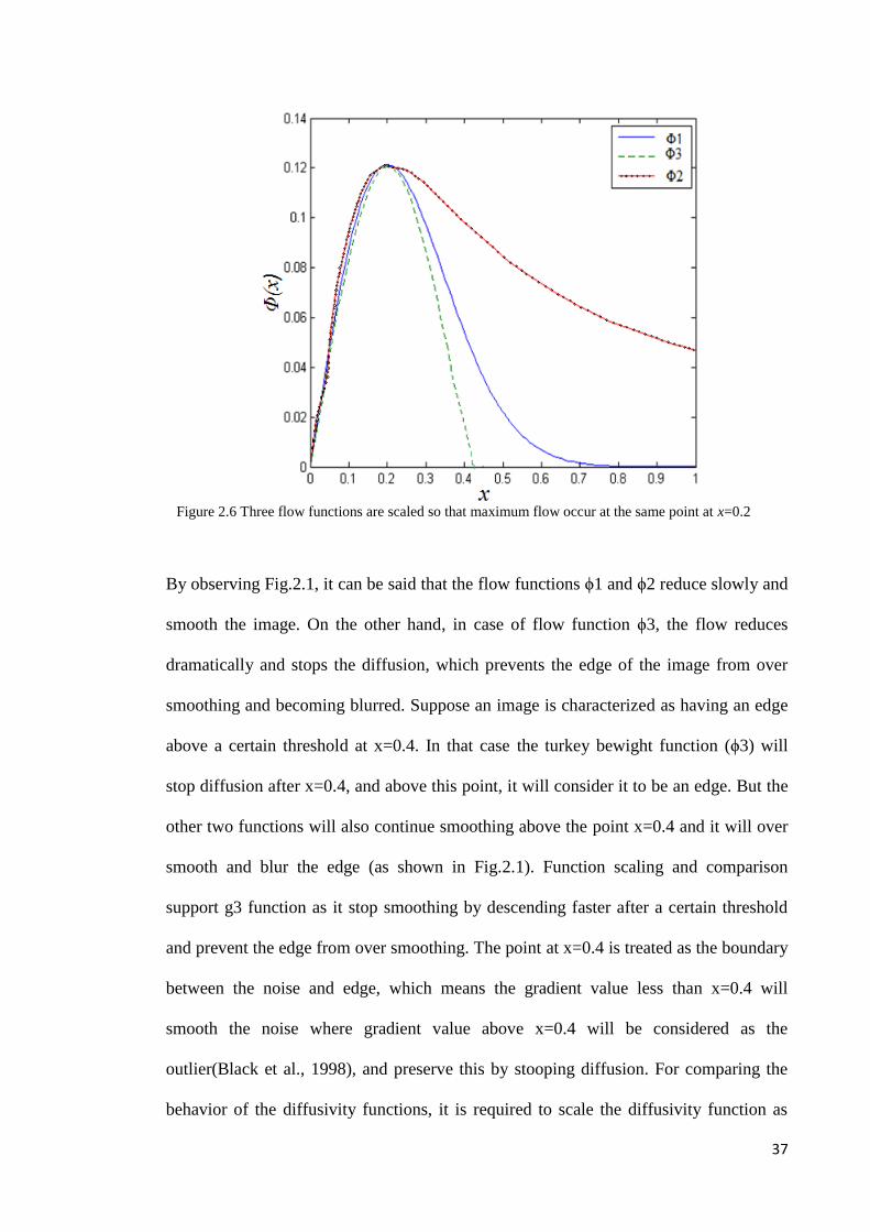
37
By observing Fig.2.1, it can be said that the flow functions ϕ1 and ϕ2 reduce slowly and
smooth the image. On the other hand, in case of flow function ϕ3, the flow reduces
dramatically and stops the diffusion, which prevents the edge of the image from over
smoothing and becoming blurred. Suppose an image is characterized as having an edge
above a certain threshold at x=0.4. In that case the turkey bewight function (ϕ3) will
stop diffusion after x=0.4, and above this point, it will consider it to be an edge. But the
other two functions will also continue smoothing above the point x=0.4 and it will over
smooth and blur the edge (as shown in Fig.2.1). Function scaling and comparison
support g3 function as it stop smoothing by descending faster after a certain threshold
and prevent the edge from over smoothing. The point at x=0.4 is treated as the boundary
between the noise and edge, which means the gradient value less than x=0.4 will
smooth the noise where gradient value above x=0.4 will be considered as the
outlier(Black et al., 1998), and preserve this by stooping diffusion. For comparing the
behavior of the diffusivity functions, it is required to scale the diffusivity function as
Figure 2.6 Three flow functions are scaled so that maximum flow occur at the same point at x=0.2
38
well as flow function to become zero at the same point. As the g2 function decreases
very slowly, it smooths the noise efficiently. As it becomes zero at infinity so its edge
preservation ability is very weak. So if it is possible to scale the function g2, so that its
value will become very low at the point where g3 is zero, then its edge preservation
ability will increase. In the proposed method, function g2 will be scaled so that its value
becomes very low at the point where g3 is zero and generates the same maximum value
as g3. The flow function ϕ2 is very efficient for smoothing speckle noise as it decreases
very slowly but is very weak for preserving edges. In this thesis the diffusivity function
g2 will be scaled, as the flow function ϕ2 descends faster to stop diffusion after a certain
threshold. G2 can preserve the edge and smooth the speckle noise simultaneously.
2.8.3.2 Gradient Threshold
The value of gradient threshold plays a vital role in effective edge detection. If
the gradient threshold is overestimated then the resultant image will be over smoothed.
On the other hand its noise reduction ability will be weakened due to underestimation of
the gradient threshold. So, selecting suitable gradient thresholds is very important for
getting a better resultant image. The gradient threshold parameters should be a
decreasing function of time, which is shown in X Li et al. (X. Li & Chen, 1994). In this
way, it can preserve the edge above a certain decreasing threshold. Gradient threshold
plays a paramount role on the performance of the diffusion process. So, selection of a
wise value of gradient threshold is required for effective noise suppression as well as
efficient edge preservation. In the case of the AD method, only one gradient threshold is
used. In the case of the proposed method, four gradient thresholds instead of one will be
used for better edge preservation and effective noise reduction.

39
2.8.3.3 Stopping criterion of AD method
The performance of the AD method also depends on the criterion to terminate
the diffusion process. It is common to terminate the diffusion process after a certain
number of iterations. As the anisotropic diffusion (AD) method is very sensitive to the
number of iterations, it is crucial to choose the exact stopping time (t). In the case of
overestimating the number of iterations, resultant images will be blurred while an
underestimating of the number of iterations will result unsatisfactory noise suppression.
For overcoming these limitations, researchers have proposed different solutions. A de-
correlation based method has been proposed by Mrazek and Navara et al. (Mrázek &
Navara, 2003). In this case, stopping time has been chosen based on when the
correlation between the noise and the signal in the output image is a minimum. In the
case of an ultrasound image this de-correlation based method is not suitable, as, in case
of US images, speckle originates from the signal. Gilboa et al. (Gilboa, Sochen, &
Zeevi, 2006) proposed a method for obtaining maximum signal to noise ratio for the
output image It. He used different equations for finding out the number of iterations for
which the SNR of the output image will be at a maximum. By using this stopping
criterion, it is possible to effectively reduce the noise of the output image but the
preservation quality of edges is not up to a standard level. Mean Absolute Error (MAE)
has been proposed by Zhang et al. (Zhang, 2007). In this case, the MAE value is used to
stop diffusion automatically between two consecutive diffusion iterations. As the MAE
criterion uses the Mean Absolute Error value between two consecutive diffusion
iteration, it is suitable for US images. Therefore, the proposed method has used this
stopping criterion.
Our AD method has been proposed by considering the gradient threshold parameters
and the diffusivity function. The goal of our method is to make a right choice and scale

40
of the diffusivity function for the AD method to obtain a better quality output image.
Proper estimation of the gradient threshold parameters has also been considered for
effective noise reduction and edge preservation.

41
CHAPTER 3
METHODOLOGY
3.1 Introduction
The main purpose of the research is to propose improvement on the quality of US
medical images by using US medical imaging to detect early knee OA. The US
medical imaging is processed by two steps (proposed HE and AD). It is known that US
medical imaging suffers from two drawbacks which are low contrast ratio and speckle
noise. The purpose of this research is to enhance the contrast of the US image, as well
as to reduce the speckle noise of the US image. This will be helpful for US imaging for
detecting early knee OA. To enhance the contrast of the US imaging Multipurpose Beta
Optimized Recursive Bi-Histogram Equalization (MBORBHE) method is used to
overcome the limitations of conventional HE method. To reduce the speckle in US
imaging, an improved AD method is used by considering two of the following three
factors which are diffusivity functions, gradient thresholds and stopping criteria which
control the effectiveness of the AD method.
3.2 Data acquisition
For data acquisition, the US images of the cartilage and the meniscus of the knee
joint. For collecting US images of knee joint cartilage, we visited University
Technology Malaysia, Johor Bahru, Malaysia. The name of the ultrasound (US)
machine was ‘aplio MX’ of TOSHIBA brand. We used a 2D, 8MHz (PLT-805AT)
linear probe for obtaining the US images. The DICOM image sizes were 528×285. We
chose linear probe to take the image of knee joint as it contained higher frequency
(8MHz) probe. An experienced and registered sonographer took the US images of the
knee joint. 20 volunteer subjects willing to give the images of their knee joint. We took
US images from different positions of the probe. The lateral side of the knee joint had

42
been given priority for imaging, as from this side, it would be possible for better
observation of the cartilage of the knee joint. We used a high frequency 8MHz probe, as
high frequency probe can give better resolution of US images. With high frequency, the
wavelength would be smaller, thus smaller imaging particles would be possible to detect
by using high frequency US probe. For the US imaging of knee joint, notch was very
important because the probe would be placed beside the patella by using notch. A
radiologist, Mr Heamn had given a lot of help in collecting the data.. The US images of
knee joint cartilage collected from UTM are shown in Fig. 3.1. The cartilage images
were taken from different positions of the knee joints.
Meanwhile, the US image of Meniscus of knee joint, were obtained from the
University of Malaya Medical Collage (UMMC). Prof. Dr. John George, a professor at
the department of Biomedical Imaging in UMMC, had helped us a lot in collecting the
US images of knee joint meniscus. Meniscus images of knee joint collected from
UMMC are shown in Fig.3.2. These images were taken from different positions of the
US probe. For this experiment we used a 6.5 MHz linear probe. Prof. Dr. John George
himself had taken the US images of knee meniscus from different position of US probe.

43
Figure 3.1: (a-g) is ultrasound images of knee joint Cartilage collected from UTM (Healthy subjects)
(a) (b)
(c) (d)
(e) (f)
(g)
Layer of cartilage

44
(a) (b) (c)
(d) (e) (f)
(g)
Figure 3.2: (a-g) is ultrasound image of knee joint Meniscus collected from UMMC (Healthy
subjects)
Meniscus
Layer of cartilage

45
3.3 US image of meniscus and cartilage of the knee joint
From Fig.3.3 shows the location of cartilage and meniscus, referred from data
which collected from the Lucile Packard Children's Hospital, Source:
http://www.daviddarling.info/encyclopedia/K/knee.html), The location of meniscus is
between the layers of cartilage. The ultrasound images may be denoted as meniscus
image or cartilage image. Though both images were taken at the knee joint, one is
named as meniscus image as a large portion of the image is covered by meniscus, as
shown in Fig.3.2. On the other hand, the other US image is named as cartilage image, as
large part of the image is covered by cartilage, as shown in Fig. 3.1.
3.4 Proposed contrast enhancement method
3.4.1 Multipurpose beta optimizes recursive bi-histogram equalization
In this study, Multipurpose Beta Optimized Recursive Bi-Histogram
Equalization (MBORBHE) method had been used for contrast enhancement of the
cartilage and meniscus US images of the knee joint. The main idea of the method was to
find out the optimum separating point for which brightness and detail preservation could
Figure 3.3 Knee joint of a normal knee

46
be achieved while enhancing the contrast of the US image. For that reason, each
possible separating point was used for decomposing the input image into two sub-
images. For converging output image mean brightness to the input image mean
brightness, recursive separation was performed. After that, conventional HE was
performed in each sub-image independently. For measuring the contrast enhancement,
detail retention and brightness preservation of the output image, three metrics were
defined. Weighted sum approach was used for constructing the final objective function
which combined the three defined metrics. The functional output was computed by
iterating each possible decomposition point for bi-histogram equalization, and resulting
image was obtained for each maximum objective function.
3.4.2 Different objective functions
In case of ideal HE, the mean brightness difference of input and output image
should be as close as possible. At the same time, it should also be able to enhance the
contrast as well as to retain the detail and preserve the brightness of the image. To
achieve this goal it had designed the objective functions to regularize different metrics.
Three metrics for the proposed method were considered, which were Preservation of
Brightness Score function (PBS), Optimum Contrast Score function (OCS), and
Preservation of Detail Score function (PDS). Beta distribution is a very well-known
distribution function. It is a versatile way to represent outcomes like probabilities or
proportions. To specify various relationships between model expert opinions and
random variables by having various functions over a certain desirable range, beta
function is very useful. Beta distribution is defined in the interval of 0 to 1. For realizing
the proposed algorithm, the beta distribution had been used. For complete model of the
final objective function, the three metrics had been combined. By using final objective
function, iteration had been performed in all possible gray levels to find the possible

47
separating gray level to maximize the objective function. Step by step construction of
different objective function is described below.
3.4.2.1 Preservation of Brightness Score function (PBS)
The first metric is regarded as Preservation of Brightness Score (PBS). This
function serves to gauge the brightness deviation of resultant image relative to input
image. This brightness deviation is modelled as the difference between the mean
illumination of input image, µ𝑥 and the mean illumination of output image µ𝒚,
µ𝑥
=1
𝑀 𝑁∑ ∑ 𝐼𝑋(𝑖,𝑗)
𝑁𝑗=0
𝑀𝐼=0 (3.1)
µ𝑦
=1
𝑀 𝑁∑ ∑ 𝐼𝑦(𝑖,𝑗)
𝑁𝑗=0
𝑀𝐼=0 (3.2)
where M represents the height of the image in term of pixels number, and N represents
the width of the image in term of pixels number. The pixel intensity in spatial location
of (i,j) in input image and output image are represented by 𝐼𝑋(𝑖,𝑗) and 𝐼𝑦(𝑖,𝑗) respectively.
Therefore, the mean illumination difference can be intuitively described as µ𝑦 − µ𝑥 .
However, this difference is not yet suitable to be used due to two problems: firstly, there
is no standard bounding value which is important to compare later with the detail
retention and enhanced contrast; secondly, it lacks of flexibility in manipulating its
expected behavior.
Hence, to resolve the first issue, it is crucial to map illumination difference score onto
the unit interval [0,1] so that the value will represent the degree of illumination
deviation instead of the absolute value of illumination difference. This mapping is
performed by using the normalization formula for relative brightness deviation as
follow. The definition of normalized brightness (NB) is

48
𝑁𝐵(µ𝑦, µ𝑥) =|µ𝑦−µ𝑥|
µ𝑥+µ𝑦+𝐶 (3.3)
where c is any arbitrary small constant used to assure computation stability in extreme
cases. The range of (3.3) is described by 𝑁𝑜𝑟𝑚(µ𝑦, µ𝑥) ∈ [0,1]. As the output value of
NB function approaches unity, it implies that the degree of deviation in brightness or
illumination between the input image and output image is high, and vice versa.
To solve the second problem of manipulating the expected behaviour, it is needed to
insert the output of (3.3) as input of another function. This function’s purpose is to
model the expected behaviour. For the sake of generality, this function is required to
exhibit different behaviours or function output’s shape by controlling only a few
parameters in order to model the expert’s opinion and knowledge conveniently. In this
case, It opted for beta distribution function with parameter 𝛼1and 𝛽1, and this function
was termed as Preservation of Brightness Score PBS:
𝑃𝐵𝑆 =𝛤(𝛼1+𝛽1)
𝛤(𝛼1)+𝛤(𝛽1)(1 − 𝑁𝐵)𝛽1−1𝑁𝐵(𝛼1−1) (3.4)
𝛤(𝑥) = ∫ 𝑒−𝑡1
0𝑁𝐵(𝑋−1)𝑑(𝑁𝐵) (3.5)
where Γ(.) is the Gamma function.
Again, to assure the output of PBS is of unit interval, it is normalized by using the
maximum value of the function as the ratio of PBS to the maximum value of PBS over
the range of NB. This normalized value of PBS is termed as the normalized
Preservation of Brightness Score, NPBS.
𝑁𝑃𝐵𝑆 =𝑃𝐵𝑆
𝑎𝑟𝑔𝑚𝑎𝑥(𝑃𝐵𝑆) (3.6)
The aim of NPBS is to model the perception of human visual system. An expert in
visual application can use it to adjust the optimum value of desired range of brightness
difference. The output value of NPBS can be viewed as the membership function of
brightness deviation value. As NPBS approaches unity, it implies that the resultant

49
image is more preferable. The parameters of NPBS, determine the location of high
values and low values of NPBS and hence determine the preference of brightness
deviation by the user.
Using PBS makes it possible to measure the difference between mean brightness of
input and output image. However, the very small brightness difference that was found in
previous researches was not able to be found by using NB. Thus, human visual
perception was not favorable in case of NB. For that reason, PBS or NPBS had been
used in this study. NPBS is a normalized function, defined as the ratio of PBS and
maximum value of PBS. In the experiment, NB was mapped by using NPBS to a new set
of value ranging from 0 to 1. Beta distribution had been used for mapping by using
parameters α1 and β1. NPBS provided us some values that were used to measure the
brightness preservation quantitatively. However, in case of traditional method, even the
smallest brightness difference would indicates the superiority of the resultant image.
Good or bad brightness preserving ability can be defined by using NPBS function with
the help of NB.
3.4.2.2 Optimum Contrast Score (OCS) function
The second metric is defined as Contrast Score (CS). This score quantifies the
degree of contrast enhancement. It is modelled by using the difference of standard
deviation of both the histogram equalized and input image. Similar to the previous
metric, the bound values of CS range are denoted as of unit interval by using parameter
𝛼2 and 𝛽2.
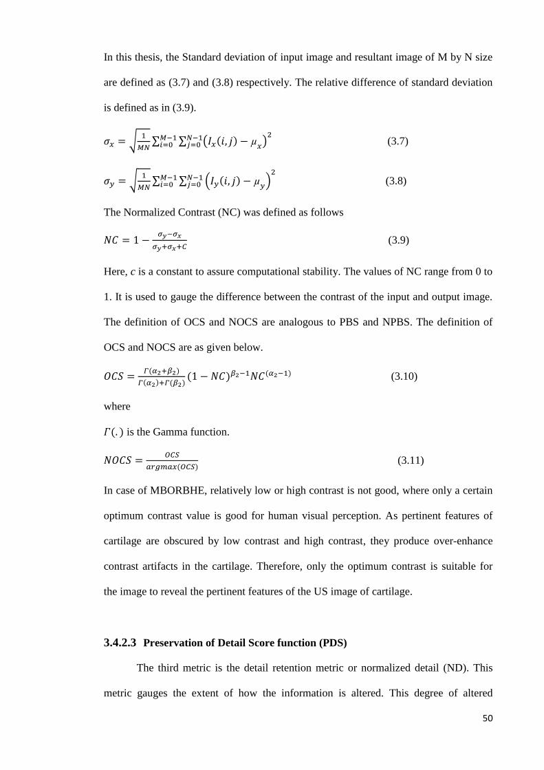
50
In this thesis, the Standard deviation of input image and resultant image of M by N size
are defined as (3.7) and (3.8) respectively. The relative difference of standard deviation
is defined as in (3.9).
𝜎𝑥 = √1
𝑀𝑁∑ ∑ (𝐼𝑥(𝑖, 𝑗) − µ
𝑥)
2𝑁−1𝑗=0
𝑀−1𝑖=0 (3.7)
𝜎𝑦 = √1
𝑀𝑁∑ ∑ (𝐼𝑦(𝑖, 𝑗) − µ
𝑦)
2𝑁−1𝑗=0
𝑀−1𝑖=0 (3.8)
The Normalized Contrast (NC) was defined as follows
𝑁𝐶 = 1 −𝜎𝑦−𝜎𝑥
𝜎𝑦+𝜎𝑥+𝐶 (3.9)
Here, c is a constant to assure computational stability. The values of NC range from 0 to
1. It is used to gauge the difference between the contrast of the input and output image.
The definition of OCS and NOCS are analogous to PBS and NPBS. The definition of
OCS and NOCS are as given below.
𝑂𝐶𝑆 =𝛤(𝛼2+𝛽2)
𝛤(𝛼2)+𝛤(𝛽2)(1 − 𝑁𝐶)𝛽2−1𝑁𝐶(𝛼2−1) (3.10)
where
𝛤(. ) is the Gamma function.
𝑁𝑂𝐶𝑆 =𝑂𝐶𝑆
𝑎𝑟𝑔𝑚𝑎𝑥(𝑂𝐶𝑆) (3.11)
In case of MBORBHE, relatively low or high contrast is not good, where only a certain
optimum contrast value is good for human visual perception. As pertinent features of
cartilage are obscured by low contrast and high contrast, they produce over-enhance
contrast artifacts in the cartilage. Therefore, only the optimum contrast is suitable for
the image to reveal the pertinent features of the US image of cartilage.
3.4.2.3 Preservation of Detail Score function (PDS)
The third metric is the detail retention metric or normalized detail (ND). This
metric gauges the extent of how the information is altered. This degree of altered
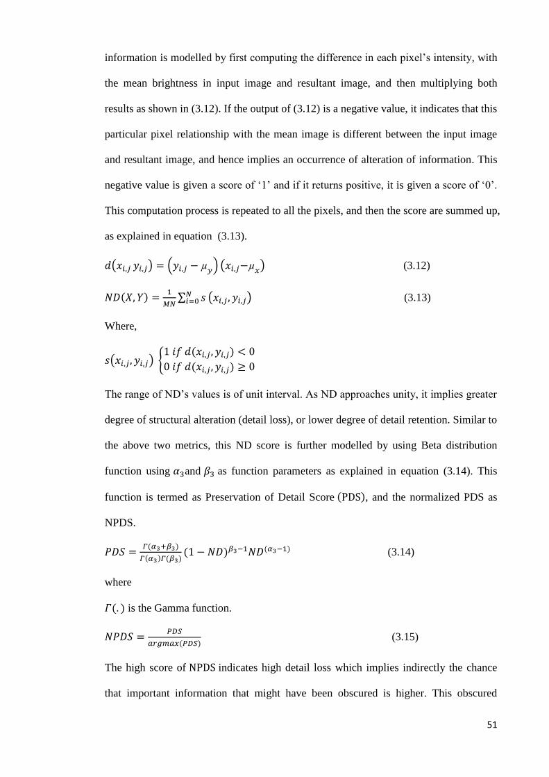
51
information is modelled by first computing the difference in each pixel’s intensity, with
the mean brightness in input image and resultant image, and then multiplying both
results as shown in (3.12). If the output of (3.12) is a negative value, it indicates that this
particular pixel relationship with the mean image is different between the input image
and resultant image, and hence implies an occurrence of alteration of information. This
negative value is given a score of ‘1’ and if it returns positive, it is given a score of ‘0’.
This computation process is repeated to all the pixels, and then the score are summed up,
as explained in equation (3.13).
𝑑(𝑥𝑖,𝑗 𝑦𝑖,𝑗) = (𝑦𝑖,𝑗 − µ𝑦
) (𝑥𝑖,𝑗−µ𝑥
) (3.12)
𝑁𝐷(𝑋, 𝑌) =1
𝑀𝑁∑ 𝑠𝑁
𝑖=0 (𝑥𝑖,𝑗 , 𝑦𝑖,𝑗) (3.13)
Where,
𝑠(𝑥𝑖,𝑗, 𝑦𝑖,𝑗) {1 𝑖𝑓 𝑑(𝑥𝑖,𝑗 , 𝑦𝑖,𝑗) < 0
0 𝑖𝑓 𝑑(𝑥𝑖,𝑗 , 𝑦𝑖,𝑗) ≥ 0
The range of ND’s values is of unit interval. As ND approaches unity, it implies greater
degree of structural alteration (detail loss), or lower degree of detail retention. Similar to
the above two metrics, this ND score is further modelled by using Beta distribution
function using 𝛼3and 𝛽3 as function parameters as explained in equation (3.14). This
function is termed as Preservation of Detail Score (PDS), and the normalized PDS as
NPDS.
𝑃𝐷𝑆 =𝛤(𝛼3+𝛽3)
𝛤(𝛼3)𝛤(𝛽3)(1 − 𝑁𝐷)𝛽3−1𝑁𝐷(𝛼3−1) (3.14)
where
𝛤(. ) is the Gamma function.
𝑁𝑃𝐷𝑆 =𝑃𝐷𝑆
𝑎𝑟𝑔𝑚𝑎𝑥(𝑃𝐷𝑆) (3.15)
The high score of NPDS indicates high detail loss which implies indirectly the chance
that important information that might have been obscured is higher. This obscured
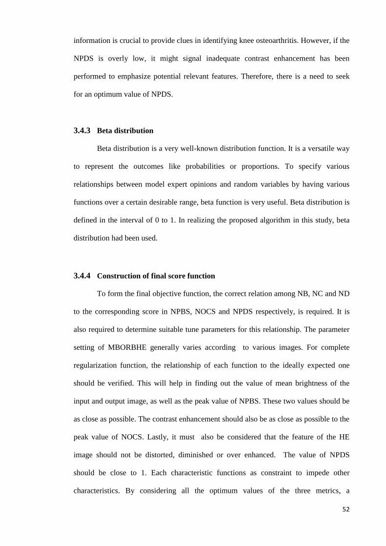
52
information is crucial to provide clues in identifying knee osteoarthritis. However, if the
NPDS is overly low, it might signal inadequate contrast enhancement has been
performed to emphasize potential relevant features. Therefore, there is a need to seek
for an optimum value of NPDS.
3.4.3 Beta distribution
Beta distribution is a very well-known distribution function. It is a versatile way
to represent the outcomes like probabilities or proportions. To specify various
relationships between model expert opinions and random variables by having various
functions over a certain desirable range, beta function is very useful. Beta distribution is
defined in the interval of 0 to 1. In realizing the proposed algorithm in this study, beta
distribution had been used.
3.4.4 Construction of final score function
To form the final objective function, the correct relation among NB, NC and ND
to the corresponding score in NPBS, NOCS and NPDS respectively, is required. It is
also required to determine suitable tune parameters for this relationship. The parameter
setting of MBORBHE generally varies according to various images. For complete
regularization function, the relationship of each function to the ideally expected one
should be verified. This will help in finding out the value of mean brightness of the
input and output image, as well as the peak value of NPBS. These two values should be
as close as possible. The contrast enhancement should also be as close as possible to the
peak value of NOCS. Lastly, it must also be considered that the feature of the HE
image should not be distorted, diminished or over enhanced. The value of NPDS
should be close to 1. Each characteristic functions as constraint to impede other
characteristics. By considering all the optimum values of the three metrics, a

53
mathematical solution has to be established. One way was to find the optimum values of
the three metrics is by finding the separating point. Nevertheless, in most cases, this is
impossible. For that reason, the best solution is to find the separating point that could
best satisfy the above mentioned criteria. The final objective function considering all
three metrics is given below
𝑁𝑂𝑏𝑗(𝑁𝐵𝑃𝑆, 𝑁𝑂𝐶𝑆, 𝑁𝐷𝑃𝑆) =𝛼(𝑁𝐵𝑃𝑆)+𝛽(𝑁𝑂𝐶𝑆)+𝛷(𝑁𝐷𝑃𝑆)
(𝛼+𝛽+𝛷) (3.16)
For all recursive HE method, the value of r=4 is usually used. In this study, different US
images of knee cartilage and meniscus were used for the performance evaluation of the
proposed method. The qualitative analysis was performed by comparing the visual
effects of different methods such as conventional HE, BBHE, DSIHE, MMBEBHE and
RSIHE with the proposed method.
3.5 Proposed AD Method
In this study, for the evaluation of the proposed AD method, the parameters of
AD method had been considered. There are three parameters that affect the efficiency of
AD method. The main effort to overcome the limitations of these three parameters to
reduce the speckle noise as well as efficiently preserve the edge of the US image. The
three parameters of the proposed AD method are described below.
3.5.1 Diffusivity function for the proposed AD method
For studying our proposed method, Catte_PM diffusion model of equation
(2.20) had been used. In this case, to automatically determine the value of σ relating to
the Gaussian noise of the image, a window size of 20⤬20 and 65⤬65 pixels was
considered. This was done to satisfy statistical calculation. By using this window size,
the most uniform block of pixels in the image could be determined. The pixel standard
deviation of each block was calculated. Finally, the standard deviation of the most
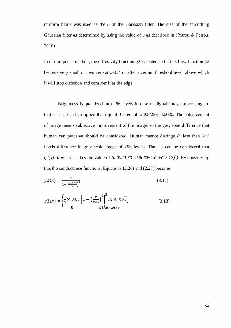
54
uniform block was used as the σ of the Gaussian filter. The size of the smoothing
Gaussian filter as determined by using the value of σ as described in (Petrou & Petrou,
2010).
In our proposed method, the diffusivity function g2 is scaled so that its flow function ϕ2
become very small or near zero at x=0.4 or after a certain threshold level, above which
it will stop diffusion and consider it as the edge.
Brightness is quantized into 256 levels in case of digital image processing. In
that case, it can be implied that digital 0 is equal to 0.5/256=0.0020. The enhancement
of image means subjective improvement of the image, so the grey tone difference that
human can perceive should be considered. Human cannot distinguish less than 2~3
levels difference in grey scale image of 256 levels. Thus, it can be considered that
g2(x)=0 when it takes the value of (0.0020)*3=0.0060~1/(1+(12.17)2). By considering
this the conductance functions, Equations (2.26) and (2.27) become
𝑔2(𝑥) =1
1+(12.17𝑥
𝑘)
2 (3.17)
𝑔3(𝑥) = {1
5× 0.67 [1 − (
𝑥
𝑘√5)
2
]2
, 𝑥 ≤ 𝑘√5
0 𝑜𝑡ℎ𝑒𝑟𝑤𝑖𝑠𝑒
, (3.18)
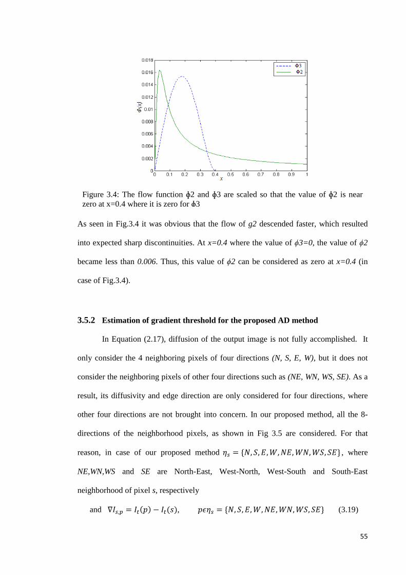
55
As seen in Fig.3.4 it was obvious that the flow of g2 descended faster, which resulted
into expected sharp discontinuities. At x=0.4 where the value of ϕ3=0, the value of ϕ2
became less than 0.006. Thus, this value of ϕ2 can be considered as zero at x=0.4 (in
case of Fig.3.4).
3.5.2 Estimation of gradient threshold for the proposed AD method
In Equation (2.17), diffusion of the output image is not fully accomplished. It
only consider the 4 neighboring pixels of four directions (N, S, E, W), but it does not
consider the neighboring pixels of other four directions such as (NE, WN, WS, SE). As a
result, its diffusivity and edge direction are only considered for four directions, where
other four directions are not brought into concern. In our proposed method, all the 8-
directions of the neighborhood pixels, as shown in Fig 3.5 are considered. For that
reason, in case of our proposed method 𝜂𝑠 = {𝑁, 𝑆, 𝐸, 𝑊, 𝑁𝐸, 𝑊𝑁, 𝑊𝑆, 𝑆𝐸} , where
NE,WN,WS and SE are North-East, West-North, West-South and South-East
neighborhood of pixel s, respectively
and ∇𝐼𝑠,𝑝 = 𝐼𝑡(𝑝) − 𝐼𝑡(𝑠), 𝑝𝜖𝜂𝑠 = {𝑁, 𝑆, 𝐸, 𝑊, 𝑁𝐸, 𝑊𝑁, 𝑊𝑆, 𝑆𝐸} (3.19)
Figure 3.4: The flow function ɸ2 and ɸ3 are scaled so that the value of ɸ2 is near
zero at x=0.4 where it is zero for ɸ3
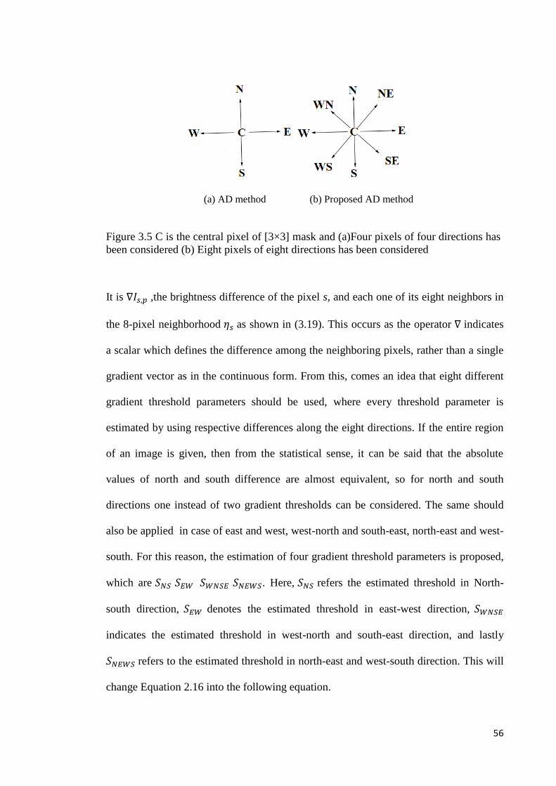
56
It is ∇𝐼𝑠,𝑝 ,the brightness difference of the pixel s, and each one of its eight neighbors in
the 8-pixel neighborhood 𝜂𝑠 as shown in (3.19). This occurs as the operator ∇ indicates
a scalar which defines the difference among the neighboring pixels, rather than a single
gradient vector as in the continuous form. From this, comes an idea that eight different
gradient threshold parameters should be used, where every threshold parameter is
estimated by using respective differences along the eight directions. If the entire region
of an image is given, then from the statistical sense, it can be said that the absolute
values of north and south difference are almost equivalent, so for north and south
directions one instead of two gradient thresholds can be considered. The same should
also be applied in case of east and west, west-north and south-east, north-east and west-
south. For this reason, the estimation of four gradient threshold parameters is proposed,
which are 𝑆𝑁𝑆 𝑆𝐸𝑊 𝑆𝑊𝑁𝑆𝐸 𝑆𝑁𝐸𝑊𝑆. Here, 𝑆𝑁𝑆 refers the estimated threshold in North-
south direction, 𝑆𝐸𝑊 denotes the estimated threshold in east-west direction, 𝑆𝑊𝑁𝑆𝐸
indicates the estimated threshold in west-north and south-east direction, and lastly
𝑆𝑁𝐸𝑊𝑆 refers to the estimated threshold in north-east and west-south direction. This will
change Equation 2.16 into the following equation.
(a) AD method (b) Proposed AD method
Figure 3.5 C is the central pixel of [3×3] mask and (a)Four pixels of four directions has
been considered (b) Eight pixels of eight directions has been considered
57
𝐼𝑇+1(𝑠) = 𝐼𝑡(𝑠) +𝜆
|𝜂𝑠|[∑ 𝑔(∇𝐼𝑆,𝑃)∇𝐼𝑆,𝑃 + ∑ 𝑔(∇𝐼𝑠,𝑝)∇𝐼𝑠,𝑝𝑝𝜖𝐸,𝑊 +𝑝𝜖𝑁,𝑆
∑ 𝑔(∇𝐼𝑠,𝑝)∇𝐼𝑠,𝑝 + ∑ 𝑔(∇𝐼𝑠,𝑝)∇𝐼𝑠,𝑝𝑝𝜖𝑊𝑁,𝑆𝐸𝑃𝜖𝑁𝐸,𝑊𝑆 ] (3.20)
In Equation 3.20 for the first 𝑔(∇𝐼𝑆,𝑃), the estimated gradient threshold is 𝑆𝑁𝑆, while for
the second 𝑔(∇𝐼𝑆,𝑃) the estimated gradient threshold is 𝑆𝐸𝑊. For the third 𝑔(∇𝐼𝑆,𝑃), the
estimated gradient threshold is 𝑆𝑁𝐸𝑊𝑆 and for the last 𝑔(∇𝐼𝑆,𝑃), the estimated gradient
threshold is 𝑆𝑊𝑁𝑆𝐸.
Estimating four gradient thresholds will give much more precise result in terms of noise
reduction and edge preservation, compared to the result of using only a single gradient
threshold vector as in continuous form. The experimental result will also be better in
term of smoothing, as smoothing that takes place for each direction is not the same. It
will vary according to the strength of difference of each direction. The gradient
threshold parameter will also vary, as larger difference will obtain higher value of S
parameter compared to other directions.
Corresponding histogram of the absolute value of the gradient component in each
direction will be used for estimating the four gradient threshold parameters. The knee
algorithm is used for finding out the threshold between two populations of histogram
having a long tail and one peak that fit with straight lines, by the sense of least square
error. After one iterative process, each population will lead to the estimation of the
threshold. Elaboration on the knee algorithm can be found in a research paper by Petrou
et al.(Petrou & Petrou, 2010).
In our method, the population has roughly flat distribution, creating long tail, which
defines the difference attribute to the true edge. On the other hand, population having
58
steeper distribution is the difference attributed to the noise. Between the two parameters,
the estimated threshold is S.
3.5.3 Stopping Criterion for the proposed AD method
In our proposed method, MAE stopping criterion is used. This process is based
on the surveillance of exponential reduction of the MAE value with the number of
iteration. When the value of MAE between two iterations is sufficiently small, the
diffusion process is terminated automatically. The MAE criterion is suitable for US
image. For this reason, this stopping criterion is used in our proposed method. For better
performance, according to the fitness of small structure of the image, different MAE
threshold should be used. In the proposed method, the MAE of the diffused image is
utilized to stop the diffusion, which is written as follows:
𝑀𝐴𝐸(𝐼𝑡) =1
𝑚×𝑛× ∑ √(𝐼𝑡
𝑖,𝑗− 𝐼𝑡−1
𝑖,𝑗)2𝑚,𝑛
(𝑖,𝑗)=1 (3.21)
where 𝐼𝑡𝑖,𝑗
and 𝐼𝑡−1𝑖,𝑗
are the filtered value of pixel (i,j) in the diffused images at time t and
t-1, respectively. The number of row and column of the diffused image are denoted by
m and n. The tissue structure and edge information are filled by the region of the
diffused image. If the values of MAE become small and stable, the diffusion terminates
and protects the diffused image from over smoothing.
3.6 Summary of the proposed AD method
Firstly, it is necessary to find out the standard deviation (σ) of the pixel within
most uniform blocks of the noisy image. The size of smoothing Gaussian filter (Gσ) is
constructed from the value of σ. Here, I0 is the original image. The number of iteration
is denoted by t. Then, It is convolved with Gσ and the values of δN*, δS*, δE*, δw*, δNE*,
δSE*, δSW* and δNW*, the differences of each pixel, are computed. After that, the method

59
is used to find out the values of δN, δS, δE, δw, δNE, δSE, δSW and δNW, which are also the
differences of each pixel by using different 2D convolution mask. Then, by using knee
algorithm, the SNS from δN and δS, SEW from δE and δw, SWNSE from δWN and δSE, SNEWS
from δNE and δWS can be estimated. By using the above values, the final diffused image
is calculated with the help of the following equation
𝐼𝑡 = 𝐼𝑡−1 +𝜆
𝜂𝑠[𝑔(𝛿𝑁∗. 𝑆𝑁𝑆)𝛿𝑁 + 𝑔(𝛿𝑆∗.𝑆𝑁𝑆)𝛿𝑆 + 𝑔(𝛿𝐸∗.𝑆𝐸𝑊)𝛿𝐸 + 𝑔(𝛿𝑊∗.𝑆𝐸𝑊)𝛿𝑊 +
𝑔(𝛿𝑊𝑁∗.𝑆𝑊𝑁𝑆𝐸)𝛿𝑊𝑁 + 𝑔(𝛿𝑆𝐸∗.𝑆𝑊𝑁𝑆𝐸)𝛿𝑆𝐸 + 𝑔(𝛿𝑊𝑆∗.𝑆𝑁𝐸𝑊𝑆)𝛿𝑊𝑆 + 𝑔(𝛿𝑁𝐸∗.𝑆𝑁𝐸𝑊𝑆)𝛿𝑁𝐸 (3.22)
Finally, the MAE value is measured for each iteration and the diffusion is terminated
when the MAE value becomes sufficiently small..
3.7 Measurement tools to assess US image quality
For quantitative analysis of the real US image, different performance metrics can
be used. The performance metrics are usually chosen based on the determination of
effectiveness of the contrast enhancement and speckle reduction methods.
3.7.1 In case of the proposed HE method
Our main objective in the proposed HE method is to preserve the brightness and
detail when enhancing the contrast of the US image. In this study, for quantitative
analysis, Signal to Noise Ratio (SNR), Structural Similarity Index Measurement (SSIM)
and Entropy had been used. SNR and Entropy had been also used for assessing the
brightness preservation and the degree of contrast enhancement, respectively. For the
measurement of the detail preservation, SSIM had been used. A bar chart of mean shift
of the original image, histogram equalized image and image of proposed method had
been also drawn for determining the ability of brightness preservation of the proposed
method.
60
Next, MSE was used to measure the effectiveness of noise reduction, by measuring the
square of difference between two images. The lower the value of MSE, the higher the
effectiveness of noise reduction will be. MSE is defined as follows:
𝑀𝑆𝐸 =1
𝑀.𝑁∑ ∑ [𝐼(𝑚, 𝑛) − 𝐼′(𝑚, 𝑛)]2𝑁−1
𝑛=0𝑀−1𝑚=0 (3.23)
Here, I is the original image, while 𝐼′ is the filtered image of different contrast
enhancement or speckle reduction method, which need to be compared for finding out
the best one. M and N are the number of rows and columns of the pixel in the images.
Here, I (m,n) indicates the input image pixel intensity at spatial location of (m,n) and
𝐼′(𝑚, 𝑛) indicates the output image pixel intensity at the spatial location of (m,n).
The definitions of SNR, SSIM and Entropy are given as follows:
𝑆𝑁𝑅 = 10 log10∑ ∑ [𝐼(𝑚,𝑛)]2𝑁−1
𝑛=0𝑀−1𝑚=0
𝑀𝑆𝐸 (3.24)
SNR is used to evaluate the standard of the output image quality. It is measured in
decibels (dB). Hence, the higher the SNR value, the better the resultant image is.
Structural Similarity Index Measurement (SSIM) is calculated on different windows of
an image. The equation for SSIM between two windows x and y of similar size is given
below:
𝑆𝑆𝐼𝑀(𝑥, 𝑦) =(2µ𝑥µ𝑦+𝐶1)(2𝜎𝑋𝑌+𝐶2)
(µ𝑥2+µ𝑦
2 +𝐶1)(𝜎𝑥2+𝜎𝑦
2+𝐶2) (3.25)
where µ𝑥 and µ𝑦 are the average of x and y respectively. 𝜎𝑥2 and 𝜎𝑦
2 are variance of x
and y respectively. 𝜎𝑋𝑌 is the co-variance of x and y. 𝐶1 and 𝐶2 are the two constants for
stabilizing the division with weak denominator, where 𝐶1 = (𝑘1𝐿)2 and 𝐶2 = (𝑘2𝐿)2. L
is the dynamic range of the pixel value, 𝑘1=0.01 and 𝑘2=0.03. The resultant of SSIM is
in decimal value and it ranges from -1 to 1. If two data sets are identical, then the result
of SSIM will be 1.
61
Entropy is used for measuring the robustness of contrast enhancement. The
mathematical equation of entropy is given below.
𝐸𝑛𝑡[𝑝] = − ∑ 𝑝(𝑘) log2 𝑝(𝑘)𝐿−1𝑘=0 (3.26)
Here in Eq. 3.26, 𝐸𝑛𝑡[𝑝] is the entropy. The probability density function (PDF) is p. L
is the number of gray level.
3.7.2 In case of Speckle noise reduction
For evaluating the performance of the proposed AD method over other AD
methods, the following performance metrics had been used: Peak signal to noise ratio
(PSNR)(Tsiotsios & Petrou, 2013), Mean Square Error (MSE)(F.Zhang, 2007a),
Structural Similarity Index Measurement (SSIM) (Wang, Bovik, Sheikh, & Simoncelli,
2004) and Pratt’s Figure of Merit (FOM)(Y. Yu, Acton, S.T., 2002). The proposed
method was then compared with conventional Perona-Malik, SRAD, LPND and NCD
method.
PSNR is used for measuring how much noise has been reduced from the noisy image.
The commonly used unity of PSNR is (dB). The Higher the value of PSNR, the larger
amount of the noise reduced from the noisy image.
𝑃𝑆𝑁𝑅 = 10 log10𝑚𝑎𝑥(𝐼(𝑚,𝑛))2
𝑀𝑆𝐸 (3.27)
SSIM is used for measuring adaptation of human visual system about the information of
structure of the scene. In this measurement method, three different important
measurements such as contrast, luminance and structure, are considered. The definition
of SSIM is given in Equation 3.25

62
For comparing the performance of edge preservation among different methods FOM is
used. FOM is defined as follows:
𝐹𝑂𝑀 =1
max {𝑁𝑟𝑒𝑎𝑙,𝑁𝑖𝑑𝑒𝑎𝑙}∑
1
1+𝑑𝑖2𝑒
𝑁𝑟𝑒𝑎𝑙𝑖=1 (3.28)
Here, Nideal and Nreal are the number of ideal and detected edge pixels. The Euclidian
distance between the nearest ideal edge pixel and ith detected edge pixel is denoted by
di. e is a constant whose value generally is 1/9. The value of FOM ranges from 0 to 1.
The higher the value of FOM, the better edge detection can be obtained.
63
CHAPTER 4 RESULT AND DISCUSSION
4.1 Introduction
In this thesis, the performance of the MBORBHE method and proposed AD
method had been evaluated qualitatively and quantitatively. In case of MBORBHE, for
qualitative and quantitative analysis, the US images of meniscus and cartilage of knee
joint had been enhanced by using contemporary contrast enhancement techniques, such
as conventional HE, BBHE, DSIHE, RSIHE, MMBEBHE and the proposed
MBORBHE method. For the evaluation of brightness preservation, the shift of mean of
conventional HE methods and proposed method from the original image had also been
evaluated. In the proposed AD method for qualitative and quantitative analysis, the real
US image of meniscus and cartilage of knee joint has also been used. The proposed AD
method had been compared with Perona-Malik, NCD, SRAD and LPND for
performance evaluation. Qualitative analysis had been performed in term of human
visual perception for both proposed HE and AD method. The quantitative analysis of
both proposed HE and AD method had been performed by using different performance
metrics such as Signal to Noise Ratio (SNR), Peak Signal to Noise Ratio (PSNR), Mean
Square Error (MSE), Figure of Merits (FOM), Structure Similarity Index Measurement
(SSIM) and Entropy. Statistical analysis had been performed on the obtained numerical
values of different performance metrics. Statistical analysis from Fisher’s Least
Significance Difference and Duncan test confirmed the best performance of the
proposed HE and AD method.
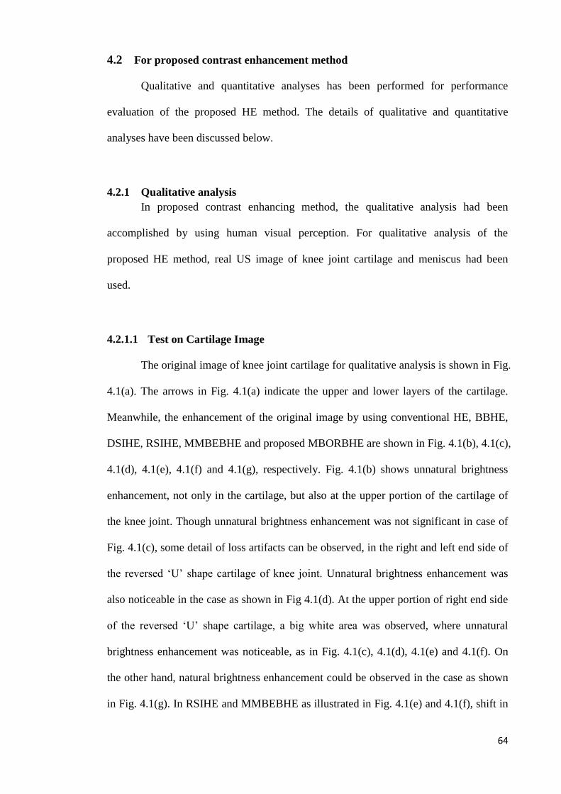
64
4.2 For proposed contrast enhancement method
Qualitative and quantitative analyses has been performed for performance
evaluation of the proposed HE method. The details of qualitative and quantitative
analyses have been discussed below.
4.2.1 Qualitative analysis
In proposed contrast enhancing method, the qualitative analysis had been
accomplished by using human visual perception. For qualitative analysis of the
proposed HE method, real US image of knee joint cartilage and meniscus had been
used.
4.2.1.1 Test on Cartilage Image
The original image of knee joint cartilage for qualitative analysis is shown in Fig.
4.1(a). The arrows in Fig. 4.1(a) indicate the upper and lower layers of the cartilage.
Meanwhile, the enhancement of the original image by using conventional HE, BBHE,
DSIHE, RSIHE, MMBEBHE and proposed MBORBHE are shown in Fig. 4.1(b), 4.1(c),
4.1(d), 4.1(e), 4.1(f) and 4.1(g), respectively. Fig. 4.1(b) shows unnatural brightness
enhancement, not only in the cartilage, but also at the upper portion of the cartilage of
the knee joint. Though unnatural brightness enhancement was not significant in case of
Fig. 4.1(c), some detail of loss artifacts can be observed, in the right and left end side of
the reversed ‘U’ shape cartilage of knee joint. Unnatural brightness enhancement was
also noticeable in the case as shown in Fig 4.1(d). At the upper portion of right end side
of the reversed ‘U’ shape cartilage, a big white area was observed, where unnatural
brightness enhancement was noticeable, as in Fig. 4.1(c), 4.1(d), 4.1(e) and 4.1(f). On
the other hand, natural brightness enhancement could be observed in the case as shown
in Fig. 4.1(g). In RSIHE and MMBEBHE as illustrated in Fig. 4.1(e) and 4.1(f), shift in

65
brightness (darker compared to other enhancement methods) was obvious, in which the
contrast decreased around the area of the cartilage.
Measuring the thickness of the cartilage required information of the exact upper and
lower edge of the cartilage. In the upper portion, a deep dark line, which was the edge of
the upper part of the cartilage, was observable. This deep dark edge was much thinner
when observed using the proposed method. This indicates that the imaging on the upper
edge of the cartilage is more precise, as can be seen in Fig. 4.1(g). The proposed method
was also more precise in case of imaging the lower portion, where it showed thinner and
more precise white dotted lines. Some unnatural white artifacts were also observable in
case of Fig. 4.1(b), 4.1(c), 4.1(d), 4.1(e) and 4.1(f). However, in case of Fig. 4.1(g),
white artefact was not observed very frequently, but a natural enhancement of the shape
of cartilage was noticed. Besides that, the reversed ‘U’ shape of the cartilage was clearly
noticeable, and there was a natural enhancement in the upper portion of the cartilage
joint. The shape of the cartilage was clearer as compared to the images taken using other
methods. In case of Fig. 4.1(b), 4.1(c), 4.1(d), 4.1(e) and 4.1(f), some unnatural tiny
white lines could be seen at the border of the cartilage, as well as at the upper portion of
the cartilage joint. It was obvious that the white border of the cartilage joint, generated
by using MBORBHE, was natural. Therefore, this method had shown to successfully
preserve the brightness and details when enhancing the contrast of the image. The
resultant images from the conventional HE, BBHE and DSIHE shown in Fig. 4.1(b),
4.1(c) and 4.1(d) also suffered from mean brightness shift, thus resulting in unpleasant
contrast enhancement. From the qualitatively analysis as shown in Fig.4.1, it can be
concluded that the proposed method can outperform the other methods.

66
4.2.1.2 Test on meniscus Image
For the qualitative analysis of the proposed HE method, the original image of
knee joint meniscus as shown in Fig. 4.2(a) and the arrows in Fig. 4.2(a) indicate the
upper and lower layer of cartilages of knee joints. The enhancement of the original
image by using conventional HE, BBHE, DSIHE, RSIHE, MMBEBHE and proposed
MBORBHE are shown in Fig. 4.2(b), 4.2(c), 4.2(d), 4.2(e), 4.2(f) and 4.2(g)
respectively. The image results from the conventional HE, BBHE and DSIHE (shown in
Fig. 4.2(b), 4.2(c) and 4.2(d)) had larger mean brightness, which were much brighter
compared to the original image, therefore they resulted in unpleasant contrast
(a) Original Image (b) Conventional HE image (c) BBHE
(d) DSIHE (e) RSIHE (f) MMBEBHE
(g) Proposed method
Figure 4.1: .(a) Original Cartilage Image (b) Conventional HE (c) BBHE (d) DSIHE (e) RSIHE (f)
MMBEBHE (g) MBORBHE (proposed)
Layer of Cartilage Unnatural Brightness
enhancement Detail loss artifacts
Big White artifacts
Natural Enhancement
Unnatural tiny white line

67
enhancement. In case of Fig. 4.2(b), unnatural brightness enhancement was observed,
not only in the meniscus, but also in the upper portion of the tibia and femur of the knee
joint. Though unnatural brightness enhancement was not so significant in case of Fig.
4.2(c), some detail loss artifacts were observed between the joint of tibia and lower part
of the ‘V’ shape cartilage. Unnatural brightness enhancement was also noticeable in
case of Fig. 4.2(d). In case of RSIHE and MMBEBHE in Fig. 4.2(e) and 4.2(f), it could
be seen that the obvious change in brightness (darker comparing with other
enhancement methods) decreased the contrast around the area of the meniscus. These
methods also gave less emphasis on detail preservation. In case of Fig. 4.2(e), detail
loss artifact in the junction of meniscus and tibia of the knee was observed. In case of
Fig. 4.2(f), the detail loss artifacts were also observable in the border of ‘V’ shaped
meniscus. However, in case of Fig. 4.2(g), the detail loss artifacts were not observed
very actively. A natural enhancement of the shape of cartilage could be seen. The ‘V’
shape of the cartilage was clearly noticeable, as shown in Fig. 4.2(g). The shape of the
meniscus collateral ligament was also clear compared to the results of other methods. In
case of Fig. 4.2(b), 4.2(c), 4.2(d), 4.2(e) and 4.2(f), some unnatural white lines at the
border of the cartilage, as well as in the meniscus could be seen. It was also observed
that the white border of the cartilage generated by the MBORBHE was natural.

68
Therefore, this proposed method has successfully preserved the brightness and
details when enhancing the contrast of the image. From the qualitative analysis as
shown in Fig.4.2, it has been proven that the proposed method can outperform the other
methods.
(a) Original Image (b) Conventional HE (c) BBHE
(d) DSIHE (e) RSIHE (f) MMBEBHE
(g)MBORBHE
Figure 4.2: (a) Original Image (b) Conventional HE (c) BBHE (d)DSIHE (e) RSIHE (f)MMBEBHE
(g) MBORBHE (proposed). (In case of meniscus image)
Femur Tibia
Layer of Cartilage
Meniscus
Detail loss artifacts
Meniscus Collateral ligament
Unnatural white line
69
Before Contrast Enhancement After Contrast Enhancement
(a) (b)
(c) (d)
(e) (f)
(g) (h)
Figure 4.3: US images of knee Meniscus for four subjects before and after contrast
enhancement are shown above (a), (b) are input and output image for subject 1. (c),
(d) are input and output image for subject 2. (e), (f) are input and output image for
subject 3, (g), (h) are input and output image for subject 4
70
The improvement of the US image of knee meniscus for different subjects after
contrast enhancement by the proposed method is shown in Fig.4.3. From the output
image as shown in Fig.4.3 (b), it can be said that the darkness of the original image had
been removed. In case of Fig.4.3 (d), it was observed that the structure of the cartilage
was much identifiable than the original image. By observing Fig.4.3 (f) and (g), it can
be concluded that not only the details of the cartilage but the contrast of the knee joint
also been significantly improved.
4.2.2 Quantitative analysis
Statistical analysis had been used for quantitative analysis of the numerical
values of different performance metrics for contrast enhancement such as SNR, SSIM,
and Entropy. The entire test was performed by using SPSS (Version 21). In this
analysis, the proposed method (MBORBHE) has been verified and tested able to
outperform the other methods.. Table 4.1 shows the mean values of SNR, SSIM and
Entropy for different contrast enhancement methods (HE, BBHE, DSIHE, RSIHE,
MMBEBHE and MBORBHE) in case of 20 healthy subjects. The mean values of SNR,
SSIM and Entropy has been compared for different HE methods. It had been shown that
the largest value of SNR was (29.177±1.585) in the proposed method, and the least
value was (21.807±0.788) in the conventional HE method. In SSIM and Entropy it
could be seen that the height values were in the proposed methods which were
(0.833±0.126) and (7.689±0.547), respectively. The least value of SSIM and Entropy
were in DSIHE and BBHE, which were (0.260±0.054) and (4.430±0.533)
respectively.As seen in Table 4.1 it was observed that MBORBHE and MMBEBHE
produced almost similar results for SSIM. The difference of mean SNR between
MMBEBHE and MBORBHE were not too large as well. Therefore, further analysis is
still required for proving the best performance of the proposed method.
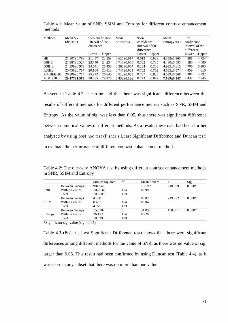
71
Table 4.1: Mean value of SNR, SSIM and Entropy for different contrast enhancement
methods
Methods Mean SNR
(dB)±SD
95% confidence
interval of the
difference
Mean
SSIM±SD
95%
confidence
interval of the
difference
Mean
Entropy±SD
95%
confidence
interval of the
difference
Lower Upper Lower Upper Lower Upper
HE 21.807±0.788 21.457 22.158 0.620±0.017 0.612 0.628 4.552±0.365 4.381 4.724
BBHE 23.987±0.527 23.740 24.234 0.718±0.035 0.702 0.735 4.430±0.533 4.180 4.680
DSIHE 24.999±0.979 24.541 25.458 0.260±0.054 0.234 0.286 4.995±0.615 4.706 5.283
RSIHE 20.458±0.757 20.104 20.813 0.747±0.031 0.732 0.762 4.635±0.374 4.459 4.810
MMBEBHE 26.306±0.714 25.972 26.640 0.813±0.055 0.787 0.839 4.559±0.368 4.387 4.732
MBORBHE 29.177±1.585 28.435 29.920 0.833±0.126 0.773 0.892 7.689±0.547 7.432 7.945
As seen in Table 4.2, it can be said that there was significant difference between the
results of different methods for different performance metrics such as SNR, SSIM and
Entropy. As the value of sig. was less than 0.05, thus there was significant difference
between numerical values of different methods. As a result, these data had been further
analyzed by using post hoc test (Fisher’s Least Significant Difference and Duncan test)
to evaluate the performance of different contrast enhancement methods.
Table 4.2: The one-way ANOVA test by using different contrast enhancement methods
in SNR, SSIM and Entropy
Sum of Squares df Mean Square F Sig.
SNR
Between Groups 984.546 5 196.909 218.929 0.000*
Within Groups 102.534 114 0.899
Total 1087.080 119
SSIM
Between Groups 4.508 5 0.902 219.972 0.000*
Within Groups 0.467 114 0.004
Total 4.975 119
Entropy
Between Groups 159.182 5 31.836 138.991 0.000*
Within Groups 26.112 114 0.229
Total 185.295 119
*Significant sig. value (sig.<0.05)
Table 4.3 (Fisher’s Lest Significant Difference test) shows that there were significant
differences among different methods for the value of SNR, as there was no value of sig.
larger than 0.05. This result had been confirmed by using Duncan test (Table 4.4), as it
was seen in any subset that there was no more than one value.

72
Table 4.3: Categorization of different methods using Fisher’s Least Significant
Difference (LSD) for SNR
(I) Method (J) Method Mean Difference
(I-J)
Std. Error Sig. 95% Confidence Interval
Lower Bound Upper Bound
HE
BBHE -2.179* 0.299 0.000 -2.773 -1.585
DSIHE -3.192* 0.299 0.000 -3.786 -2.597
RSIHE 1.349* 0.299 0.000 0.755 1.943
MMBEBHE -4.498* 0.299 0.000 -5.092 -3.904
MBORBHE -7.369* 0.299 0.000 -7.964 -6.775
BBHE
HE 2.179* 0.299 0.000 1.585 2.773
DSIHE -1.012* 0.299 0.001 -1.606 -0.418
RSIHE 3.528* 0.299 0.000 2.934 4.122
MMBEBHE -2.318* 0.299 0.000 -2.913 -1.724
MBORBHE -5.190* 0.299 0.000 -5.784 -4.596
DSIHE
HE 3.192* 0.299 0.000 2.597 3.786
BBHE 1.012* 0.299 0.001 0.418 1.606
RSIHE 4.541* 0.299 0.000 3.947 5.135
MMBEBHE -1.306* 0.299 0.000 -1.900 -0.712
MBORBHE -4.177* 0.299 0.000 -4.772 -3.583
RSIHE
HE -1.349* 0.299 0.000 -1.943 -0.755
BBHE -3.528* 0.299 0.000 -4.122 -2.934
DSIHE -4.541* 0.299 0.000 -5.135 -3.947
MMBEBHE -5.847* 0.299 0.000 -6.441 -5.253
MBORBHE -8.719* 0.299 0.000 -9.313 -8.125
MMBEBHE
HE 4.498* 0.299 0.000 3.904 5.092
BBHE 2.318* 0.299 0.000 1.724 2.913
DSIHE 1.306* 0.299 0.000 0.712 1.900
RSIHE 5.847* 0.299 0.000 5.253 6.441
MBORBHE -2.871* 0.299 0.000 -3.465 -2.277
MBORBHE
HE 7.369* 0.299 0.000 6.775 7.964
BBHE 5.190* 0.299 0.000 4.596 5.784
DSIHE 4.177* 0.299 0.000 3.583 4.772
RSIHE 8.719* 0.299 0.000 8.125 9.313
MMBEBHE 2.871* 0.299 0.000 2.277 3.465
*The mean difference is significant at the 0.05 level.
Table 4.4: Categorization of contrast enhancement methods into homogenous subset
using the Duncan test for SNR
Method N Subset for alpha = 0.05
1 2 3 4 5 6
RSIHE 20 20.458
HE 20 21.807
BBHE 20 23.987
DSIHE 20 24.999
MMBEBHE 20 26.306
MBORBHE 20 29.177
Sig. 1.000 1.000 1.000 1.000 1.000 1.000
Means for groups in homogeneous subsets are displayed.
Uses Harmonic Mean Sample Size = 20.000.
Fisher’s Least Significant different test as shown in Table 4.5 indicates that the mean
difference between BBHE and RSIHE was -0.029 and was 0.029 between RSIHE and
BBHE. The mean difference between MMBEBHE and MBORBHE was -0.019 and was
0.019 between MBORBHE and MMBEBHE. From these data, it can be said that there
was no significant mean difference between the values of SSIM in case of BBHE and
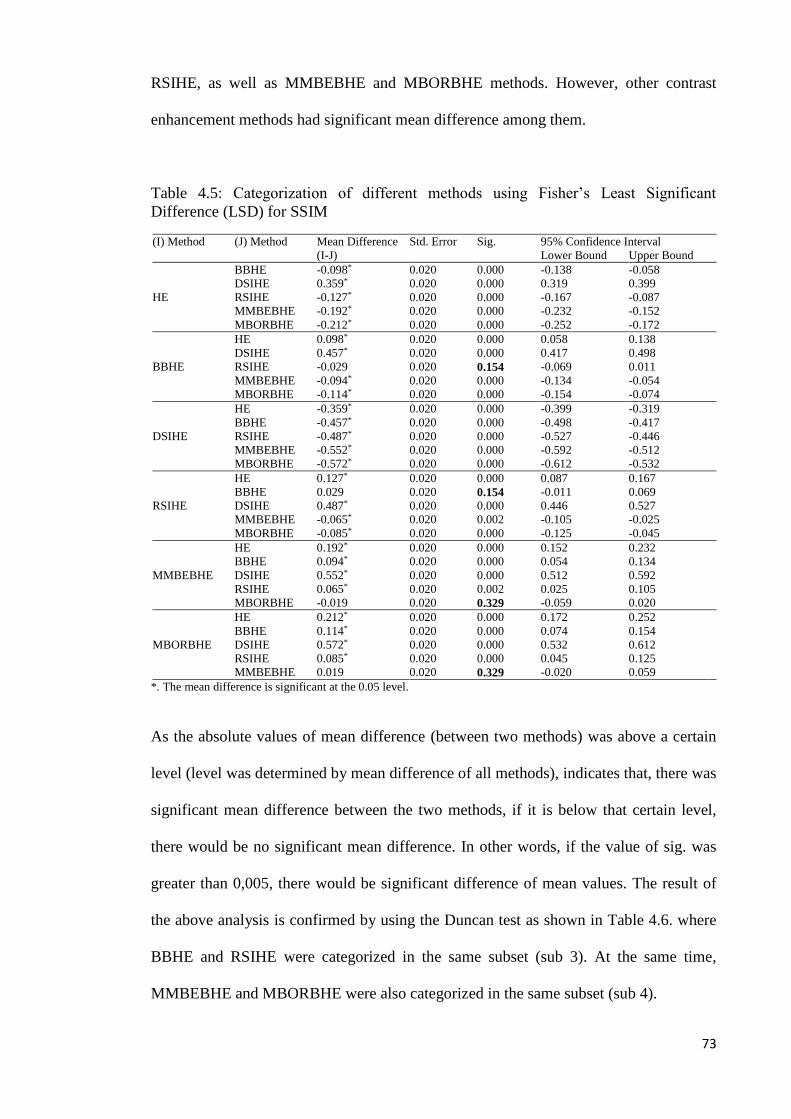
73
RSIHE, as well as MMBEBHE and MBORBHE methods. However, other contrast
enhancement methods had significant mean difference among them.
Table 4.5: Categorization of different methods using Fisher’s Least Significant
Difference (LSD) for SSIM
(I) Method (J) Method Mean Difference
(I-J)
Std. Error Sig. 95% Confidence Interval
Lower Bound Upper Bound
HE
BBHE -0.098* 0.020 0.000 -0.138 -0.058
DSIHE 0.359* 0.020 0.000 0.319 0.399
RSIHE -0.127* 0.020 0.000 -0.167 -0.087
MMBEBHE -0.192* 0.020 0.000 -0.232 -0.152
MBORBHE -0.212* 0.020 0.000 -0.252 -0.172
BBHE
HE 0.098* 0.020 0.000 0.058 0.138
DSIHE 0.457* 0.020 0.000 0.417 0.498
RSIHE -0.029 0.020 0.154 -0.069 0.011
MMBEBHE -0.094* 0.020 0.000 -0.134 -0.054
MBORBHE -0.114* 0.020 0.000 -0.154 -0.074
DSIHE
HE -0.359* 0.020 0.000 -0.399 -0.319
BBHE -0.457* 0.020 0.000 -0.498 -0.417
RSIHE -0.487* 0.020 0.000 -0.527 -0.446
MMBEBHE -0.552* 0.020 0.000 -0.592 -0.512
MBORBHE -0.572* 0.020 0.000 -0.612 -0.532
RSIHE
HE 0.127* 0.020 0.000 0.087 0.167
BBHE 0.029 0.020 0.154 -0.011 0.069
DSIHE 0.487* 0.020 0.000 0.446 0.527
MMBEBHE -0.065* 0.020 0.002 -0.105 -0.025
MBORBHE -0.085* 0.020 0.000 -0.125 -0.045
MMBEBHE
HE 0.192* 0.020 0.000 0.152 0.232
BBHE 0.094* 0.020 0.000 0.054 0.134
DSIHE 0.552* 0.020 0.000 0.512 0.592
RSIHE 0.065* 0.020 0.002 0.025 0.105
MBORBHE -0.019 0.020 0.329 -0.059 0.020
MBORBHE
HE 0.212* 0.020 0.000 0.172 0.252
BBHE 0.114* 0.020 0.000 0.074 0.154
DSIHE 0.572* 0.020 0.000 0.532 0.612
RSIHE 0.085* 0.020 0.000 0.045 0.125
MMBEBHE 0.019 0.020 0.329 -0.020 0.059
*. The mean difference is significant at the 0.05 level.
As the absolute values of mean difference (between two methods) was above a certain
level (level was determined by mean difference of all methods), indicates that, there was
significant mean difference between the two methods, if it is below that certain level,
there would be no significant mean difference. In other words, if the value of sig. was
greater than 0,005, there would be significant difference of mean values. The result of
the above analysis is confirmed by using the Duncan test as shown in Table 4.6. where
BBHE and RSIHE were categorized in the same subset (sub 3). At the same time,
MMBEBHE and MBORBHE were also categorized in the same subset (sub 4).

74
Table 4.6: Categorization of contrast enhancement methods into homogenous subset
using the Duncan test for SSIM
Method N Subset for alpha = 0.05
1 2 3 4
DSIHE 20 0.260
HE 20 0.620
BBHE 20 0.718
RSIHE 20 0.747
MMBEBHE 20 0.813
MBORBHE 20 0.833
Sig. 1.000 1.000 0.154 0.329
Means for groups in homogeneous subsets are displayed.
Uses Harmonic Mean Sample Size = 20.000.
Fisher Least Significant test as shown in Table 4.7 shows that the mean difference
between HE and BBHE was 0.122 (-0.122 between BBHE and HE), -0/082 between HE
and RSIHE (0.082 between RSIHE and HE), -0.007 between HE and MMBEBHE
(0.007 between MMBEBHE and HE). From these values, it can be said that there was
no significant difference for HE and BBHE, HE and RSIHE, HE and MMBEBHE, as
the values of sig, for these methods were larger than 0.05. However other contrast
enhancement methods had significant difference of the numerical values of entropy.
Table 4.7: Categorization of different methods using Fisher’s Least Significance
Difference (LSD) for Entropy
(I) Method (J) Method Mean Difference
(I-J)
Std.
Error
Sig. 95% Confidence Interval
Lower Bound Upper Bound
HE
BBHE 0.122 0.151 0.420 -0.177 0.422
DSIHE -0.442* 0.151 0.004 -0.742 -0.142
RSIHE -0.082 0.151 0.588 -0.382 0.217
MMBEBHE -0.007 0.151 0.963 -0.306 0.292
MBORBHE -3.136* 0.151 0.000 -3.436 -2.836
BBHE
HE -0.122 0.151 0.420 -0.422 0.177
DSIHE -0.564* 0.151 0.000 -0.864 -0.265
RSIHE -0.204 0.151 0.179 -0.504 0.095
MMBEBHE -0.129 0.151 0.394 -0.429 0.170
MBORBHE -3.258* 0.151 0.000 -3.558 -2.959
DSIHE
HE 0.442* 0.151 0.004 0.142 0.742
BBHE 0.564* 0.151 0.000 0.265 0.864
RSIHE 0.360* 0.151 0.019 0.060 0.659
MMBEBHE 0.435* 0.151 0.005 0.135 0.735
MBORBHE -2.693* 0.151 0.000 -2.99 -2.394

75
RSIHE
HE 0.082 0.151 0.588 -0.217 0.382
BBHE 0.204 0.151 0.179 -0.095 0.504
DSIHE -0.360* 0.151 0.019 -0.659 -0.060
MMBEBHE 0.075 0.151 0.620 -0.224 0.375
MBORBHE -3.054* 0.151 0.000 -3.353 -2.754
MMBEBHE
HE 0.007 0.151 0.963 -0.292 0.306
BBHE 0.129 0.151 0.394 -0.170 0.429
DSIHE -0.435* 0.151 0.005 -0.735 -0.135
RSIHE -0.075 0.151 0.620 -0.375 0.224
MBORBHE -3.129* 0.151 0.000 -3.429 -2.829
MBORBHE
HE 3.136* 0.151 0.000 2.836 3.436
BBHE 3.258* 0.151 0.000 2.959 3.558
DSIHE 2.693* 0.151 0.000 2.394 2.993
RSIHE 3.054* 0.151 0.000 2.754 3.353
MMBEBHE 3.129* 0.151 0.000 2.829 3.429
*The mean difference is significant at the 0.05 level.
This result was confirmed by using the Duncan test as shown in Table 4.8, where HE,
BBHE, RSIHE, MMBEBHE were categorized in the same subset.
Table 4.8: Categorization of contrast enhancement methods into homogenous subset
using Duncan test for Entropy
Method N Subset for alpha = 0.05
1 2 3
BBHE 20 4.430
HE 20 4.552
MMBEBHE 20 4.559
RSIHE 20 4.635
DSIHE 20 4.995
MBORBHE 20 7.689
Sig. .223 1.000 1.000
Means for groups in homogeneous subsets are displayed.
Uses Harmonic Mean Sample Size = 20.000.
According to the result computed by using the values of SNR, SSIM and Entropy, the
performance of the contrast enhancement methods were ranked as in Table 4.9. The
ranking were done based on the result of Duncan test as shown in Table 4.4, 4.6 and 4.8.
As seen in Table 4.4, it was observed that the mean value of SNR for every method are
in different subset, therefore, these six methods had been ranked in a descending order
from 1 to 6 according to their mean values. Table 4.6 shows that the mean values of
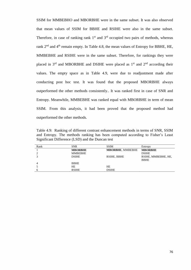
76
SSIM for MMBEBHO and MBORBHE were in the same subset. It was also observed
that mean values of SSIM for BBHE and RSIHE were also in the same subset.
Therefore, in case of ranking rank 1st and 3rd occupied two pairs of methods, whereas
rank 2nd and 4th remain empty. In Table 4.8, the mean values of Entropy for BBHE, HE,
MMBEBHE and RSIHE were in the same subset. Therefore, for rankings they were
placed in 3rd and MBORBHE and DSIHE were placed as 1st and 2nd according their
values. The empty space as in Table 4.9, were due to readjustment made after
conducting post hoc test. It was found that the proposed MBORBHE always
outperformed the other methods consistently.. It was ranked first in case of SNR and
Entropy. Meanwhile, MMBEBHE was ranked equal with MBORBHE in term of mean
SSIM. From this analysis, it had been proved that the proposed method had
outperformed the other methods.
Table 4.9: Ranking of different contrast enhancement methods in terms of SNR, SSIM
and Entropy. The methods ranking has been computed according to Fisher’s Least
Significant Difference (LSD) and the Duncan test
Rank SNR SSIM Entropy
1 MBORBHE MBORBHE, MMBEBHE MBORBHE
2 MMBEBHE DSIHE
3 DSIHE RSIHE, BBHE RSIHE, MMBEBHE, HE,
BBHE
4 BBHE
5 HE HE
6 RSIHE DSIHE
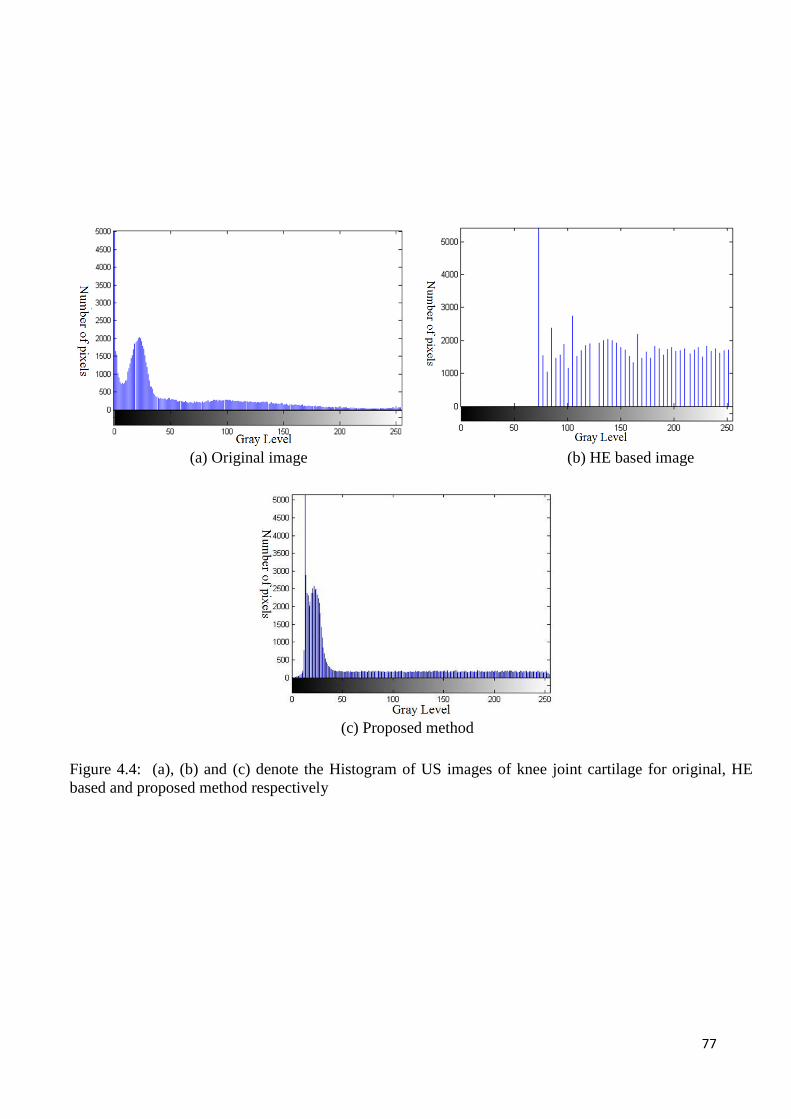
77
(a) Original image (b) HE based image
(c) Proposed method
Figure 4.4: (a), (b) and (c) denote the Histogram of US images of knee joint cartilage for original, HE
based and proposed method respectively
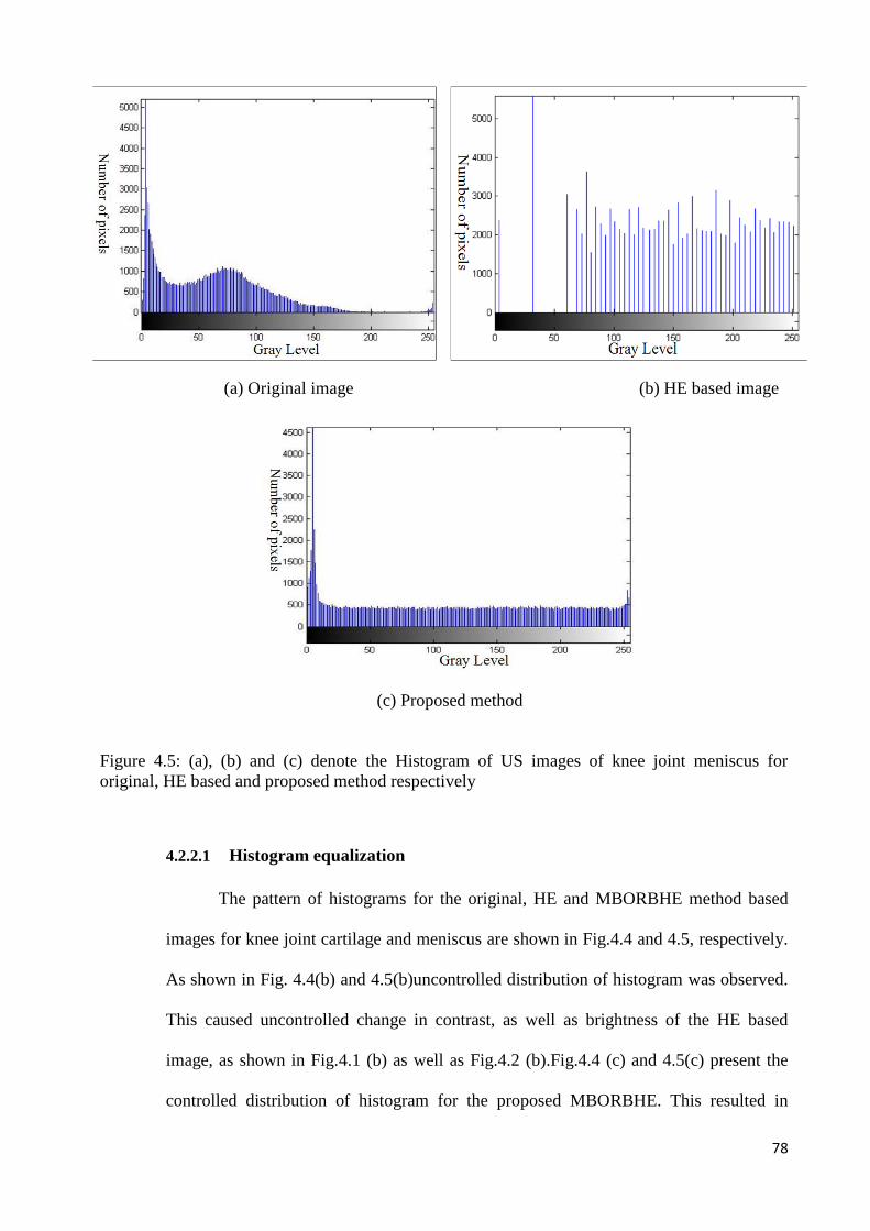
78
4.2.2.1 Histogram equalization
The pattern of histograms for the original, HE and MBORBHE method based
images for knee joint cartilage and meniscus are shown in Fig.4.4 and 4.5, respectively.
As shown in Fig. 4.4(b) and 4.5(b)uncontrolled distribution of histogram was observed.
This caused uncontrolled change in contrast, as well as brightness of the HE based
image, as shown in Fig.4.1 (b) as well as Fig.4.2 (b).Fig.4.4 (c) and 4.5(c) present the
controlled distribution of histogram for the proposed MBORBHE. This resulted in
(a) Original image (b) HE based image
(c) Proposed method
Figure 4.5: (a), (b) and (c) denote the Histogram of US images of knee joint meniscus for
original, HE based and proposed method respectively

79
expected contrast enhancement and brightness preservation of the proposed method, as
shown in Fig. 4.1(g) and 4.2(g).
4.2.2.2 Mean shift
One of the most encountered problem of HE based enhancement is the mean
shift (mean brightness change) of the output images. It happens as intensity value is
redistributed at the time of intensity normalization. The above bar chart shows the
comparison of mean shift of the proposed method with the original image and HE based
image. As seen in Fig.. 4.6 it was clear that HE based method dramatically changed the
original mean of the input image, which degraded the brightness of the original image.
However, by using the proposed MBORBHE method, it was seen that the mean value
was almost equal to the mean value of the original image. This characteristic of the
proposed MBORBHE method preserved the brightness of the original image. Therefore,
the proposed method is better for brightness preservation compared with other HE
methods.
Figure 4.6: Mean of original, HE and Proposed HE method
0
20
40
60
80
100
120
140
Cartilage Image Meniscus Image
Mean (Originall Image) Mean (HE based Image)
Mean (proposed method)
Bri
gh
tnes
s
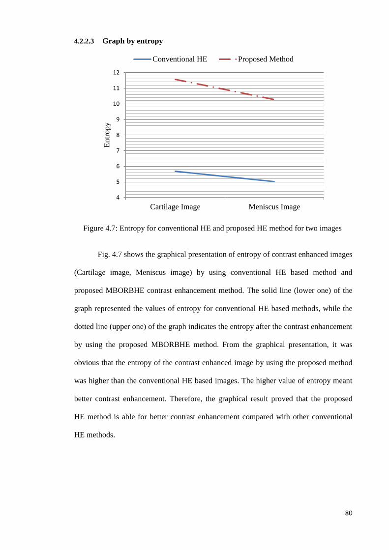
80
4.2.2.3 Graph by entropy
Fig. 4.7 shows the graphical presentation of entropy of contrast enhanced images
(Cartilage image, Meniscus image) by using conventional HE based method and
proposed MBORBHE contrast enhancement method. The solid line (lower one) of the
graph represented the values of entropy for conventional HE based methods, while the
dotted line (upper one) of the graph indicates the entropy after the contrast enhancement
by using the proposed MBORBHE method. From the graphical presentation, it was
obvious that the entropy of the contrast enhanced image by using the proposed method
was higher than the conventional HE based images. The higher value of entropy meant
better contrast enhancement. Therefore, the graphical result proved that the proposed
HE method is able for better contrast enhancement compared with other conventional
HE methods.
Figure 4.7: Entropy for conventional HE and proposed HE method for two images
4
5
6
7
8
9
10
11
12
Cartilage Image Meniscus Image
Entr
opy
Conventional HE Proposed Method
81
4.3 For proposed AD method
For the performance evaluation of the proposed AD method, qualitative and
quantitative analyses had been performed. Qualitative analysis was accomplished by
using human visual perception, while quantitative analysis was done by using different
performance metrics such as PSNR, SSIM, and FOM.
4.3.1 Qualitative analysis
For the performance evaluation of the proposed AD method, the qualitative
analysis of real US image of knee joint cartilage and meniscus had been performed. The
proposed method had been compared with different contemporary AD method such as
Perona-Malik, NCD SRAD and LPND for qualitative performance evaluation. The
qualitative analysis of US images are discussed below.
Firstly, the advantage of using proposed diffusivity function and four gradient
thresholds has been confirmed by using the proposed diffusivity function and four
gradient threshold separately, in case of conventional AD method. After that, the better
performance of the proposed method for speckle noise reduction and edge preservation
was evaluated in case of real US image of knee joint cartilage and meniscus.
For the evaluation of edge preservation ability of the proposed g2 function, AD filtering
with g2 and g3 diffusivity function had been used, in case of simulated US image as
shown in Fig.4.8 Ultrasound model described by Yu et al. (Y. Yu, Acton, S.T., 2002)
had been used to simulate the images. Fig. 4.8(a) shows the original image and Fig.
4.8(b) shows the simulated US image. As seen in Fig.4.8(c) and (d), it was also clear
that the speckle noise reduction and edge preservation ability of the g2 function were
much better than those of g3 function. Here, t=30 and k=0.4 had been used. As seen in

82
Fig. 4.8, it was clear that the performance of the conductance function g2 was much
better than that of g3 for edge preservation and speckle noise reduction.
For finding out the advantage of using four gradient threshold over one and two,
portion of the seismic image for AD filtering with one, two and four gradient thresholds
had been used. Fig. 4.9(a) shows the original image and Fig. 4.9(b) shows AD filtering
by using one gradient threshold. Fig. 4.9 (c) and (d) show AD filtering from the use of
two and four gradient thresholds, respectively. By comparing the line indicated by the
arrows as Fig. 4.9(c) and (d) then it was observed that the starting and the middle of this
line were much blurred compared to those as shown in Fig. 4.9(d). This phenomenon
was observable in other places as well. Therefore as seen in Fig. 4.9, it can be said that
the edge preservation in Fig.4.9 (d) was much better than the edge preservation as
shown in Fig.4.9 (b) and Fig.4.9 (c). From Fig. 4.9, it can also be said that selecting one
or two gradient threshold value S overestimated the threshold value between true edge
and noise. This over estimation resulted in quick degradation (over smoothing) of the
image edge, as shown in Fig.4.9 (b) and (c). From these it was clear that our proposed
method was much better in preserving edge while reducing the speckle noise of the US
image, as it had used four gradient thresholds instead of one.
(a) (b) (c) (d)
Figure 4.8: (a) original image. (b) Simulated ultrasound image (c) AD filtering using
g2 after 30 iterations (d) AD filtering using g3 after 30 iteration

83
It is known that the gradient threshold should show decreasing function of time with the
number of iterations. As shown in Fig.4.10 it was obvious that gradient threshold
parameters showed decreasing function of time. It was also observed that the gradient
Figure 4.10: The estimation of one gradient threshold parameter S, two gradient threshold parameters
SNS, SEW, and estimation of four threshold parameters SWNSE and SNEWS of Fig. 4.9 in every iteration with
the help of knee algorithm
(a) (b) (c) (d)
Figure 4.9: (a) Portion of seismic image. (b) Filtered version with estimated one gradient threshold S after 10
iterations. (c) Filtered version with estimated two gradient threshold after 10 iterations. (d) Filtered version
with estimated four gradient threshold

84
threshold estimated for SWNSE in every iteration was much higher than those in SNS, SWE,
and SWSNE. The reason for this was that most edges of figure as shown inFig.4.9 were
oriented from west-South to North-East direction. Thus, the strength of difference was
higher in case of west-North to South-East direction. Larger difference in that direction
would certainly obtain higher value of S for that direction.
4.3.1.1 Test on Cartilage Image
Fig. 4.11(a) shows the US image of knee joint cartilage. The arrows in Fig.4.11
(a) (Male, 35) indicate the upper layer and lower layer of the cartilage of knee joint. The
image as shown in Fig. 4.11(b) was over smoothed, due to overestimation of the
gradient threshold, as a result of using only one gradient threshold. The reversed ‘U’
shape cartilage was fully blurred. Underestimation of gradient threshold was observable,
as shown in Fig. 4.11(c) and (d). As a result, the speckle noise was not removed
efficiently. These figures were a little bit blurred compare to these in Fig.4.11 (f). As
shown in Fig. 4.11(e), the overestimation of gradient threshold which degraded the edge
preservation ability of the filter was observed. It also remove the important details of the
US image. By observing the output image of the proposed method of Fig. 4.11(f), it can
be concluded that edge preservation and noise reduction have been better performed
simultaneously.

85
4.3.1.2 Test on Meniscus Image
Fig. 4.12(a) shows the original US image (Male, 27) of knee joint meniscus. The
arrows in Fig.4.12 (a) indicate the upper layer and lower layer of the cartilage of knee
joint. Fig. 4.12(b), (c), (d) and (e) shows the resultant images of different speckle
reduction methods, named as PM, SRAD, NCD and LPND. Fig. 4.12(f) shows the
images result for the proposed method. The image as shown in Fig. 4.12(b) is over
smooth which degraded the preservation ability of the edge, over estimating the gradient
threshold. The ‘V’ shape cartilage is fully blurred. Fig. 4.12(c) shows an underestimated
gradient threshold as some noise was left compared with Fig.4.12 (f). As shown in Fig.
4.12(d) it was observed that the edge preservation as well as noise smoothing were both
(a) Original Image (b) Perona Malik
(c) SRAD (d) NCD
(e) LPND (f) Proposed
Figure 4.11: US Image of Cartilage for AD (a) Original Image. Resultant image of AD
filtered image by using (b) Perona Malik method (c) SRAD method (d) Non-Linear
Complex Diffusion method (NCD) (e) LPND (f) Proposed method.
Layer of cartilage Reversed ‘U’ shape cartilage

86
deteriorating. Some important details had also been removed. The shape of cartilage
also became blurred. Fig. 4.12(e) also shows poor edge preservation ability. The
degradation of ‘V’ shape cartilage was fully noticeable. It also removed important
details of the US image. Nevertheless, as shown in Fig 4.12(f) it was seen that by using
four gradient thresholds and the proposed diffusivity function, it was possible to reduce
the noise effectively and preserve the edge of the image efficiently.
Figure 4.12: US image of cartilage for medial side of knee joint for AD (a) Original Image. Resultant
image of AD filter by using (b) Perona Malik method (c) SRAD method (d) Non-Linear Complex
Diffusion method (NCD) (e) LPND (f) Proposed method.
(a) Original Image (b) Perona Malik (c) SRAD
(d) NCD (e) LPND (f) Proposed
Layer of cartilage
Degradation of ‘V’ shape cartilage

87
4.3.2 Quantitative analysis
Different diffusion methods had also been compared for the quantitative
analysis, by using different performance metrics (PSNR, SSIM and FOM) for real
ultrasound images. Statistical analysis had been performed by using IBM SPSS statistic
(version 21). In this analysis, it was shown that the proposed speckle reduction method
outperformed others methods. Three quantitative metrics, namely PSNR, SSIM and
FOM had been used for the performance analysis of the proposed method.
Table 4.10: Mean value of PSNR, SSIM and FOM with standard deviation for PM,
LPND, NCD, SRAD and proposed method
Method Mean
PSNR±SD
95% confidence
interval of
difference
Mean
SSIM±SD
95% confidence
interval of
difference
Mean
FOM±SD
95% confidence
interval of
difference
Lower
Bound
Upper
Bound
Lower
Bound
Upper
Bound
Lower
Bound
Upper
Bound
Perona-
Malik
23.088±1.227 22.514 23.663 0.732±0.065 0.702 0.762 0.443±0.056 0.416 0.469
LPND 25.403±0.816 25.021 25.785 0.803±0.038 0.785 0.821 0.480±0.035 0.463 0.496
NCD 25.236±0.793 24.865 25.608 0.850±0.026 0.838 0.863 0.559±0.040 0.540 0.579
SRAD 27.328±0.693 27.003 27.653 0.854±0.018 0.846 0.862 0.671±0.010 0.566 0.577
Proposed 31.509±1.045 31.020 31.999 0.866±0.027 0.853 0.878 0.712±0.046 0.690 0.734
Table 4.10 shows the mean value of PSNR, SSIM and FOM for the filtered US image
of 20 healthy subjects for different filtering methods. In case of PSNR and FOM, the
height values were 31.509±1.045 and 0.712±0.046. These values were obtained for the
proposed AD method. The least values of PSNR and FOM were in case of conventional
Perona –Malik (PM) method, which were 23.088±1.227 and 0.443±0.056, respectively,
In case of SSIM and FOM, the values for NCD, SRAD and proposed method were
almost similar. As the values of different performance metrics for SRAD and proposed
method were almost similar, further analysis was also performed to test our hypothesis.
Table 4.11: The one-way ANOVA computed by using different speckle reduction
methods in PSNR, FOM and SSIM
Sum of Squares df Mean Square F Sig.
PSNR Between Groups 804.378 4 201.095 229.710 0.000*
Within Groups 83.166 95 0.875
Total 887.544 99
FOM Between Groups 0.864 4 0.216 129.222 0.000*
Within Groups 0.159 95 0.002
Total 1.023 99
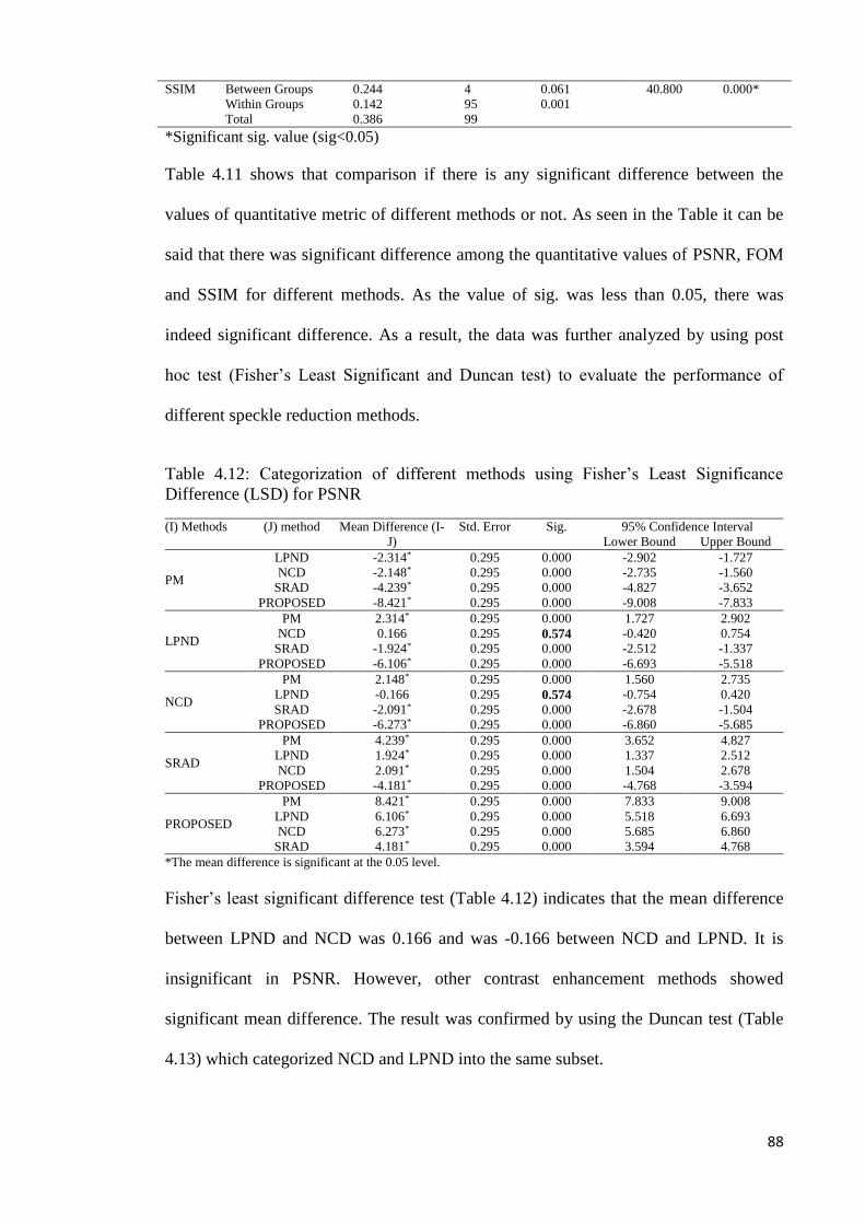
88
SSIM Between Groups 0.244 4 0.061 40.800 0.000*
Within Groups 0.142 95 0.001
Total 0.386 99
*Significant sig. value (sig<0.05)
Table 4.11 shows that comparison if there is any significant difference between the
values of quantitative metric of different methods or not. As seen in the Table it can be
said that there was significant difference among the quantitative values of PSNR, FOM
and SSIM for different methods. As the value of sig. was less than 0.05, there was
indeed significant difference. As a result, the data was further analyzed by using post
hoc test (Fisher’s Least Significant and Duncan test) to evaluate the performance of
different speckle reduction methods.
Table 4.12: Categorization of different methods using Fisher’s Least Significance
Difference (LSD) for PSNR
(I) Methods (J) method Mean Difference (I-
J)
Std. Error Sig. 95% Confidence Interval
Lower Bound Upper Bound
PM
LPND -2.314* 0.295 0.000 -2.902 -1.727
NCD -2.148* 0.295 0.000 -2.735 -1.560
SRAD -4.239* 0.295 0.000 -4.827 -3.652
PROPOSED -8.421* 0.295 0.000 -9.008 -7.833
LPND
PM 2.314* 0.295 0.000 1.727 2.902
NCD 0.166 0.295 0.574 -0.420 0.754
SRAD -1.924* 0.295 0.000 -2.512 -1.337
PROPOSED -6.106* 0.295 0.000 -6.693 -5.518
NCD
PM 2.148* 0.295 0.000 1.560 2.735
LPND -0.166 0.295 0.574 -0.754 0.420
SRAD -2.091* 0.295 0.000 -2.678 -1.504
PROPOSED -6.273* 0.295 0.000 -6.860 -5.685
SRAD
PM 4.239* 0.295 0.000 3.652 4.827
LPND 1.924* 0.295 0.000 1.337 2.512
NCD 2.091* 0.295 0.000 1.504 2.678
PROPOSED -4.181* 0.295 0.000 -4.768 -3.594
PROPOSED
PM 8.421* 0.295 0.000 7.833 9.008
LPND 6.106* 0.295 0.000 5.518 6.693
NCD 6.273* 0.295 0.000 5.685 6.860
SRAD 4.181* 0.295 0.000 3.594 4.768
*The mean difference is significant at the 0.05 level.
Fisher’s least significant difference test (Table 4.12) indicates that the mean difference
between LPND and NCD was 0.166 and was -0.166 between NCD and LPND. It is
insignificant in PSNR. However, other contrast enhancement methods showed
significant mean difference. The result was confirmed by using the Duncan test (Table
4.13) which categorized NCD and LPND into the same subset.
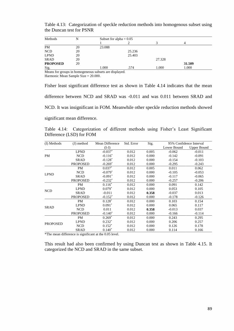
89
Table 4.13: Categorization of speckle reduction methods into homogenous subset using
the Duncan test for PSNR
Methods N Subset for alpha = 0.05
1 2 3 4
PM 20 23.088
NCD 20 25.236
LPND 20 25.403
SRAD 20 27.328
PROPOSED 20 31.509
Sig. 1.000 .574 1.000 1.000
Means for groups in homogeneous subsets are displayed.
Harmonic Mean Sample Size = 20.000.
Fisher least significant difference test as shown in Table 4.14 indicates that the mean
difference between NCD and SRAD was -0.011 and was 0.011 between SRAD and
NCD. It was insignificant in FOM. Meanwhile other speckle reduction methods showed
significant mean difference.
Table 4.14: Categorization of different methods using Fisher’s Least Significant
Difference (LSD) for FOM
(I) Methods (J) method Mean Difference
(I-J)
Std. Error Sig. 95% Confidence Interval
Lower Bound Upper Bound
PM
LPND -0.037* 0.012 0.005 -0.062 -0.011
NCD -0.116* 0.012 0.000 -0.142 -0.091
SRAD -0.128* 0.012 0.000 -0.154 -0.103
PROPOSED -0.269* 0.012 0.000 -0.295 -0.243
LPND
PM 0.037* 0.012 0.005 0.011 0.062
NCD -0.079* 0.012 0.000 -0.105 -0.053
SRAD -0.091* 0.012 0.000 -0.117 -0.065
PROPOSED -0.232* 0.012 0.000 -0.257 -0.206
NCD
PM 0.116* 0.012 0.000 0.091 0.142
LPND 0.079* 0.012 0.000 0.053 0.105
SRAD -0.011 0.012 0.358 -0.037 0.013
PROPOSED -0.152* 0.012 0.000 -0.178 -0.126
SRAD
PM 0.128* 0.012 0.000 0.103 0.154
LPND 0.091* 0.012 0.000 0.065 0.117
NCD 0.011 0.012 0.358 -0.013 0.037
PROPOSED -0.140* 0.012 0.000 -0.166 -0.114
PROPOSED
PM 0.269* 0.012 0.000 0.243 0.295
LPND 0.232* 0.012 0.000 0.206 0.257
NCD 0.152* 0.012 0.000 0.126 0.178
SRAD 0.140* 0.012 0.000 0.114 0.166
*The mean difference is significant at the 0.05 level.
This result had also been confirmed by using Duncan test as shown in Table 4.15. It
categorized the NCD and SRAD in the same subset.

90
Table 4.15: Categorization of speckle reduction methods into homogenous subset using
the Duncan test for FOM
Methods N Subset for alpha = 0.05
1 2 3 4
PM 20 0.443
LPND 20 0.480
NCD 20 0.559
SRAD 20 0.571
PROPOSED 20 0.712
Sig. 1.000 1.000 0.358 1.000
Means for groups in homogeneous subsets are displayed.
Uses Harmonic Mean Sample Size = 20.000.
Fisher’s least significant difference test as shown in Table 4.16 indicates that the mean
difference between NCD and SRAD was -0.003 and was 0.003 between SRAD and
NCD. The difference between NCD and PROPOSED was -0.015 and was 0.015
between PROPOSED and NCD. At the same time, the difference between PROPOSED
and SRAD is 0.011 and was -0.011 between SRAD and PROPOSED. These were
insignificant in SSIM. Other speckle reduction methods showed significant mean
difference. The result had been confirmed by using the Duncan test as shown in Table
4.17.
Table 4.16: Categorization of different methods using Fisher’s Least Significance
Difference (LSD) for SSIM
(I) Methods (J) method Mean Difference
(I-J)
Std. Error Sig. 95% Confidence Interval
Lower Bound Upper Bound
PM
LPND -0.070* 0.012 0.000 -0.095 -0.046
NCD -0.118* 0.012 0.000 -0.142 -0.093
SRAD -0.122* 0.012 0.000 -0.146 -0.097
PROPOSED -0.133* 0.012 0.000 -0.157 -0.109
LPND
PM 0.070* 0.012 0.000 0.046 0.095
NCD -0.047* 0.012 0.000 -0.071 -0.023
SRAD -0.051* 0.012 0.000 -0.075 -0.026
PROPOSED -0.062* 0.012 0.000 -0.086 -0.038
NCD
PM 0.118* 0.012 0.000 0.093 0.142
LPND 0.047* 0.012 0.000 0.023 0.071
SRAD -0.003 0.012 0.759 -0.028 0.020
PROPOSED -0.015 0.012 0.210 -0.039 0.008
SRAD
PM 0.122* 0.012 0.000 0.097 0.146
LPND 0.051* 0.012 0.000 0.026 0.075
NCD 0.003 0.012 0.759 -0.020 0.028
PROPOSED -0.011 0.012 0.342 -0.035 0.012
PROPOSED
PM 0.133* 0.012 0.000 0.109 0.157
LPND 0.062* 0.012 0.000 0.038 0.086
NCD 0.015 0.012 0.210 -0.008 0.039
SRAD 0.011 0.012 0.342 -0.012 0.035
*The mean difference is significant at the 0.05 level.

91
Table 4.17: Categorization of speckle reduction methods into homogenous subset using
Duncan’s test for SSIM
Methods N Subset for alpha = 0.05
1 2 3
PM 20 0.732
LPND 20 0.803
NCD 20 0.850
SRAD 20 0.854
PROPOSED 20 0.866
Sig. 1.000 1.000 0.238
Means for groups in homogeneous subsets are displayed.
Harmonic Mean Sample Size = 20.000.
The performance of the different speckle reduction methods (PM, LPND, NCD, SRAD
and PROPOSED) had been ranked by using the result computed from PSNR, SSIM and
FOM. Table 4.18 showed the rank of different methods. Some empty spaces that as in
Table 4.18 were the readjustment made after conducting post hoc test. It had been
observed that the proposed method outperformed other methods constantly in all the test
and was ranked first in PSNR and FOM. However, in SSIM other two methods namely
SRAD and NCD also were ranked equal to the proposed method. It was also observed
that the conventional Perona-Malik (PM) model always remained at the bottom of the
ranking, meaning that it faced a lot of limitations for reducing speckle and edge
preserving of the US image.
Table 4.18: Ranking of methods in terms of peak PSNR, SSIM and FOM. The method
ranking is computed according to Fisher’s Least Significance Difference (LSD) and the
Duncan test.
Rank PSNR SSIM FOM
1 PROPOSED PROPOSED, SRAD, NCD PROPOSED
2 SRAD SRAD, NCD
3 NCD, LPND
4 LPND LPND
5 PM PM PM
All experiments were conducted on a PC with 3.0-GHz Core i5 processor in
Matlab 7.9.0 (R2009b). This software had also been used for studying different
graphical output. It took 10s, 26s, 9s, 24s and 44s for Perona-Malik, SRAD, CND,
LPND and proposed method. For the proposed method it took much longer time as
larger computation needed to be is performed.

92
CHAPTER 5
CONCLUSION AND FUTURE WORK
5.1 Conclusion
This thesis has successfully solved the limitations of US imaging in terms of low
contrast and speckle noise. For contrast enhancement, it has used an effective contrast
enhancing method named MBORBHE, which enhanced the contrast of the US images,
considering detail and brightness preservation. For speckle noise reduction, it has used
an improved AD method by developing a new diffusivity function and considering four
gradient thresholds instead of one. The proposed contrast enhancing method gives
emphasis on the selection of an optimum separating point used for segmenting the
histogram of the image. This optimum separating point could be obtained from the three
regularization functions. The proposed MBORBHE method was able to preserve better
details and brightness during the contrast enhancement of the US image, outperforming
other conventional HE methods. In the case of the proposed AD method, which is by
using a new diffusivity function and four gradient threshold instead of one, it is able to
reduce the speckle noise effectively as well as preserve the edge of the image
successfully. For a suitable stopping time for iterations it has used a MAE stopping
criterion between two consecutive diffusion iterations that will stop the diffusion
automatically. In this thesis, in the proposed HE and AD method, performance has been
evaluated qualitatively and quantitatively. This task has been accomplished by
comparing different HE and AD methods with the proposed HE and AD method. Real
ultrasound images of knee joint meniscus and cartilage have been used for the
performance evaluation of the proposed HE and AD method. Qualitative analysis has
been performed by using human visual perception. From qualitative observation, it can
be concluded that the proposed MBORBHE method was able to preserve brightness and
details, when contrast is being enhanced. On the other hand, the other methods only

93
consider either brightness or detail preservation while ignoring the other one. The
proposed AD method which combine three steps mentioned above, also showed better
performance that other diffusion methods, not only qualitatively but also quantitatively.
The qualitative analysis proves that the proposed AD method outperforms other
conventional AD methods in terms of speckle noise reduction and edge preservation.
Statistical analysis has been performed for the quantitative analysis for the proposed HE
and AD method. The statistical result that has been obtained from Fisher’s Least
Significance Difference test and Duncan test consistently proves that the proposed HE
and AD method outperform other methods.
The proposed HE and AD method can also be used in the case of other medical
imaging systems, for the improvement of image quality, such as MRI, X-ray and C.T.
The output-improved image of the proposed method could have potentiality for
detecting other joint OA as well. Lastly, it can be said that in any kind of medical
imaging, for any kind of diagnosis, the proposed method will be helpful.
5.2 Limitation of the proposed method
The main idea of the proposed HE method is to find out the separating point for
segmenting the histogram of the input image for which the brightness and detail
preservation difference between the contrasts enhanced image and the original image is
at its lowest level and the contrast enhancement is at its peak. Sometimes more than one
point may be obtained for this, however the output result for the each point of optimum
values is not same. So, selecting an accurate point is a limitation of the proposed
method. In the proposed AD method, there are only two improved parameters; the
diffusivity function, and the gradient threshold. It does not improve the other parameters
such as stopping criterion for the proposed AD method. In this study, it used the US
94
images of 20 healthy subjects. No osteoarthritis US image has used for the contrast
enhancement and speckle noise reduction. Clinical evaluation for detection of OA has
not also been performed for our proposed method. Therefore, it does not evaluate the
osteoarthritis detection parameters, such as reflection coefficient and attenuation by
using different filtering methods. The proposed method only improves the US image of
knee joint cartilage, which can be helpful for detecting early knee OA.
5.3 Future work
In the proposed HE method, brightness and detail preservation has been
considered during the contrast enhancement of the images. For that reason three
objective functions have been considered, viz. Preservation of Brightness Score function
(PBS), Optimum Contrast Score function (OCS), and Preservation of Detail Score
function (PDS). For future work, Preservation of Edge Score function (PES) should be
included with the three objective functions to obtain a better output image. In the
proposed AD method future work, there will be development of a better stopping
criterion that will be suitable for US images and stop the iterations automatically. The
future work will also include the use of proposed HE and AD method in US images of
knee joint cartilage for OA cases. By using this filtering method, the thickness,
sharpness and grey level of cartilage can also be measured, as this filter may reduce the
speckle noise and preserve the edge of US cartilage image. The output of the US image
will be used for accomplishing the clinical evaluation of the proposed method.
95
REFERENCES
A. Lopes, R. T., E. Nezry. (1990). Adaptive speckle filters and scene heterogeneity.
Geosci. Remote Sens, 28, 992-1000.
A.Achim, A. B. (2001). Novel bayesian multiscale method for speckle removal
inmedical ultrasound images. Med.Imaging, 20(8), 772–783.
A.Achim, A. B. (2001). Novel bayesian multiscale method for speckle removal
inmedical ultrasound images. Med.Imaging, 20(8), 772-783.
A.J. Teichtahl, A. E. W., M.L. Davies-Tuck, F.M. Cicuttini. (2008). Best Practice &
Research Clinical Rheumatology. Imaging of knee osteoarthritis, 22, 1061-1074.
A.K.Jain. (1989). Fundamentals of Digital Image Processing. Prentice-Hallof India.
A. Achim, Bezerianos, A., & Tsakalides, P. (2001). Novel Bayesian multiscale method
for speckle removal in medical ultrasound images. Medical Imaging, IEEE
Transactions on, 20(8), 772-783.
D. Adam, Beilin-Nissan, S., Friedman, Z., & Behar, V. (2006). The combined effect of
spatial compounding and nonlinear filtering on the speckle reduction in
ultrasound images. Ultrasonics, 44(2), 166-181.
A Shanks Huynh, D. F. A., Monica S. Torres, Margaret K. Baldwin, Robert J. Gillies,
David L. Morse. (2011). Development of an Orthotopic Human Pancreatic
Cancer Xenograft Model Using Ultrasound Guided Injection of Cells. PLoS
ONE, 6(5), 1-9.
B.Sahiner. (2007). Malignant and benign breast masses on 3D US volumetric images:
effect of computer-aided diagnosis on radiologist accuracy. Radiology, 242(3),
716-724.
B.Sahiner. (2008). Malignant and benign breast masses on 3D US volumetric images:
effect of computer-aided diagnosis on radiologist accuracy. Radiology, 242(3),
316-320.
V. Behar, Adam, D., & Friedman, Z. (2003). A new method of spatial compounding
imaging. Ultrasonics, 41(5), 377-384.
M. Black, J., Sapiro, G., Marimont, D. H., & Heeger, D. (1998). Robust anisotropic
diffusion. Image Processing, IEEE Transactions on, 7(3), 421-432.
H. Bliddal, Boesen, M., Christensen, R., Kubassova, O., & Torp-Pedersen, S. (2008).
Imaging as a follow-up tool in clinical trials and clinical practice. Best Practice
& Research Clinical Rheumatology, 22(6), 1109-1126.
JM. Bremner, L. J., Miall WE. (1968). Degenerative joint disease in a Jamaican rural
population. Annals of the Rheumatic Diseases, 27(4), 326-332.
A. Buades, Coll, B., & Morel, J.-M. (2005). A review of image denoising algorithms,
with a new one. Multiscale Modeling & Simulation, 4(2), 490-530.
96
J. A. Buckwalter, & Martin, J. A. (2006). Osteoarthritis. Advanced Drug Delivery
Reviews, 58(2), 150-167. doi: http://dx.doi.org/10.1016/j.addr.2006.01.006
C. B. Burckhardt,. (1978). Speckle in ultrasound B-mode scans. Sonics and Ultrasonics,
IEEE Transactions on, 25(1), 1-6.
C.B.Burckhardt. (1987). Speckle in ultrasound B-mode scans. Sonics Ultrason., 25(1),
1-6.
CD Control. (2003) Public health and aging: Projected prevalence of self reported
arthritis or chronic joint symptoms among persons aged 65 years in United
States, 2005-2030.. MMWR Morb Mortal Wkly Rep,, 52(21), 489-491.
D.-R. Chen,., Chang, R.-F., Chen, C.-J., Ho, M.-F., Kuo, S.-J., Chen, S.-T., . . . Moon,
W. K. (2005). Classification of breast ultrasound images using fractal feature.
Clinical imaging, 29(4), 235-245.
R. N. Czerwinski,., Jones, D. L., & O'Brien, W. (1999). Detection of lines and
boundaries in speckle images-application to medical ultrasound. Medical
Imaging, IEEE Transactions on, 18(2), 126-136.
D. Adam, E. E., Y.Y. Schechner. (2006). Ultrasound image denoising by spatially
varying frequency compounding. Lecture Notes on Computer Science, 41(47), 1-
10.
D.T. Kuan, A. A. S., T.C. Strand, P. Chavel. (1987). Adaptive restoration of images
with speckle. Acoust. Speech Signal Process. ASSP, 35, 373-383.
MA. Davis, E. W., Neuhaus JM, Hauck WW. (1988). Sex differences in osteoarthritis
of the knee. The role of obesity. American Journal of Epidemiology, 127(5),
1019-1030.
L. Douglas. Miller, C. D., Dorothy Sorenson, Ming Liu. (2011). Histological
Observation of Islet Hemorrhage Induced by Diagnostic Ultrasound with
Contrast Agent in Rat Pancreas. PLoS ONE, 6(6), 1-7.
F. Eckstein, C. F., Raynauld J, Waterton JC, Peterfy C. (2006). Magnetic resonance
imaging (MRI) of articular cartilage in knee osteoarthritis (OA): morphological
assessment. Osteoarthr Cartil 2006;, 14((Suppl A)), 46–75.
E. Michael Jung, C. F., Patrick Hoffstetter, Lena Marie Dendl, Frank Klebl, Ayman
Agha, Phillipp Wiggermann, Christian Stroszcynski, Andreas Georg Schreyer.
(2012). Volume Navigation with Contrast Enhanced Ultrasound and Image
Fusion for Percutaneous Interventions: First Results. PLoS ONE, 7(3), 1-7.
J. Evans, P. O., Godber, S. X., & Robinson, M. (1994). Three-dimensional x-ray display
techniques. Paper presented at the IS&T/SPIE 1994 International Symposium on
Electronic Imaging: Science and Technology.
F.Catte´ , P. L., J.Morel,T.Coll. (1992). Image selective smoothing and edge detection
by nonlinear diffusion. SIAM J. Numer. Anal., 29, 182-193.

97
F.Zhang, Y. M. Y., L.M.Koh,Y.Kim,. (2007a). Nonlinear diffusion in Laplacian
pyramid domain for ultrasonic speckle reduction. IEEETrans.Med.Imag, 26,
200–211.
F.Zhang, Y. M. Y., L.M.Koh,Y.Kim,. (2007b). Nonlinear diffusion in laplacian pyramid
domain for ultrasonic speckle reduction. Med.Imaging, 26(2), 207-2011.
Farshad-Amacker, N. A., Lurie, B., Herzog, R. J., & Farshad, M. (2013). Interreader
and intermodality reliability of standard anteroposterior radiograph and magnetic
resonance imaging in detection and classification of lumbosacral transitional
vertebra. The Spine Journal.
DT. Felson, N. A., Anderson J, Kazis L, Castelli W, Meenan RF:. (1987). The
prevalence of knee osteoarthritis in the elderly. The Framingham Osteoarthritis
Study. Arthritis and Rheumatism, 30, 914-918.
V. Frost, S., Stiles, J. A., Shanmugan, K. S., & Holtzman, J. (1982). A model for radar
images and its application to adaptive digital filtering of multiplicative noise.
Pattern Analysis and Machine Intelligence, IEEE Transactions on(2), 157-166.
F. kwok, C. C. a. D. N. H. (1983). Comprise of Several Techniques to Obtain Multiple
Look SAR Imagery IEEE Transac. on Geosci and Remote Sensing, , 21(3), 666-
671.
G, ter. Haar. (2007). Therapeutic applications of ultrasound. Prog Biophys Mol Bio, 93,
111-129.
G.Gilboa, N. S., Y.Y.Zeevi,. (2004). Image enhancement and denoising by complex
diffusion process. IEEETrans.PatternAnal.Mach.Intell, 26, 1020–1036.
LR. Gavrilov, T. E., Davies IA. (1996). Application of focused ultrasound for the
stimulation of neural structures. Ultrasound Med Biol, 22, 179–192.
G. Gerig,., Kubler, O., Kikinis, R., & Jolesz, F. A. (1992). Nonlinear anisotropic
filtering of MRI data. Medical Imaging, IEEE Transactions on, 11(2), 221-232.
T. Gibson, H. K., Kadir M, Sultana S, Fatima Z, Syed A. Knee pain amongst the poor
and affluent in Pakistan. British Journal of Rheumatology 1996, 35(2), 146-149.
G. Gilboa, Sochen, N., & Zeevi, Y. Y. (2006). Estimation of optimal PDE-based
denoising in the SNR sense. Image Processing, IEEE Transactions on, 15(8),
2269-2280.
H.D.Cheng, J. S., W.Ju,Y.Guo,L.Zhang. (2010). Automated breast cancer detection and
classification using ultrasound images: a survey,. Pattern Recognition, 43(1),
299-317.
H.D.Cheng, J. S., W.Ju,Y.Guo,L.Zhang. (2010). Automated breast cancer detection and
classification using ultrasound images: a survey,. Pattern Recognition,, 43(1),
299-317.
HA, Valkenburg. (1980). Clinical versus radiological osteoarthritis in the general
population. In: Peyron JG, editor. Epidemiology of osteoarthritis. Paris: Ciba-
Geigy,, 53-58.

98
D. Hamerman. (1995). Clinical implications of osteoarthritis and aging. Annals of the
Rheumatic Diseases, 54, 82-85.
J. Hillary Braun a, c., Garry E. Gold. (2012). Diagnosis of osteoarthritis: Imaging.
Bone., 51, 278-288.
H K., S. N. Choi. (2008). Brightness preservaing weight clustering histogram
eualization. IEEE Trans. Consumer Electronics, 54, 1329-1337.
D..Hunter, J, Lo, G. H., Gale, D., Grainger, A. J., Guermazi, A., & Conaghan, P. G.
(2008). The reliability of a new scoring system for knee osteoarthritis MRI and
the validity of bone marrow lesion assessment: BLOKS (Boston–Leeds
Osteoarthritis Knee Score). Annals of the rheumatic diseases, 67(2), 206-211.
K. Maurer,. Basic data on arthritis: knees, hip and sacro-iliac joints. Adults ages 25-74
years. United States 1971-1975. U.S. Department of Health, Education and
Welfare.
JE, Kennedy. (2005). High-intensity focused ultrasound in the treatment of solid
tumours. Nat Rev Cancer, 5, 321-327.
S. Jespersen, Wilhjelm, J., & Sillese, H. (1998). Multi-angle compounding imaging.
Ultrasonic Imaging, 20(2), 81-102.
C. Kelsy, (2002). Medical Imaging Physics. 4th ed. Health Phys, 86(6), 912-921.
K.Z.Abd-Elmoniem, A. M. Y., Y.M.Kadah. (2002). Real-time speckle reduction and
coherence enhancement in ultrasound imaging via nonlinear anisotropic
diffusion. IEEE Trans. Biomed. Eng, 49, 997–1014.
M. Karaman,., Kutay, M. A., & Bozdagi, G. (1995). An adaptive speckle suppression
filter for medical ultrasonic imaging. Medical Imaging, IEEE Transactions on,
14(2), 283-292.
H. Keen, Wakefield, R., & Conaghan, P. (2009). A systematic review of
ultrasonography in osteoarthritis. Annals of the rheumatic diseases, 68(5), 611-
619.
M. Kim, M. C. (2008). Recursively separated and weighted histogram equalization for
brightness preservation and contrast enhancement. iEEE Trans. Consumer
Electronics, 54, 1389–1397.
T. Kim, P. J. (2008). Adaptive contrast enhancement using gain-controllable clipped
histogram equalization. IEEE Trans. Consumer Electronics, 54, 1803-1810.
Y.-T. Kim:, (1997). Contrast enhancement using brightness preserving bi-histogram
equalization. IEEE Trans. Consumer Electronics, 43(1), 1-8.
K. Krissian, & Aja-Fernández, S. (2009). Noise-driven anisotropic diffusion filtering of
MRI. Image Processing, IEEE Transactions on, 18(10), 2265-2274.
K. Krissian, Westin, C.-F., Kikinis, R., & Vosburgh, K. G. (2007). Oriented speckle
reducing anisotropic diffusion. Image Processing, IEEE Transactions on, 16(5),
1412-1424.

99
D. Kuan,. T., Sawchuk, A., Strand, T. C., & Chavel, P. (1987). Adaptive restoration of
images with speckle. Acoustics, Speech and Signal Processing, IEEE
Transactions on, 35(3), 373-383.
L, Carmona. The prevalence of 6 rheumatic disease in the Spanish population. Annals of
the Rheumatic Diseases 2000;.
L. Menashe yz, K. H. z., E. Losina x, M. Kloppenburg k, W. Zhang , L. Li z, D.J.
Hunter. (2012). Osteoarthritis and Cartilage." The diagnostic performance of
MRI in osteoarthritis: a systematic review and meta-analysis. Osteoarthritis and
Cartilage, 20, 13-21.
L.C.Gupta, A. G. (1998). X-ray Diagnosis and Imaging,. thirded.,JayPee Brothers
Medical Publishers, NewDelhi, India.
S. Lau, (1994). Global image enhancement using local information. Electronics Letters,
30(2), 122-123.
J.-S. Lee, (1980). Digital image enhancement and noise filtering by use of local
statistics. Pattern Analysis and Machine Intelligence, IEEE Transactions on(2),
165-168.
J. Lee, S. (1986). Speckle suppression and analysis for synthetic aperture radar.
Optim.Eng., 25(5), 636-643.
Li, F.-K., Croft, C., & Held, D. N. (1983). Comparison of several techniques to obtain
multiple-look SAR imagery. Geoscience and Remote Sensing, IEEE
Transactions on(3), 370-375.
Li, X., & Chen, T. (1994). Nonlinear diffusion with multiple edginess thresholds.
Pattern Recognition, 27(8), 1029-1037.
T. Loupas,., McDicken, W., & Allan, P. (1989). An adaptive weighted median filter for
speckle suppression in medical ultrasonic images. Circuits and Systems, IEEE
Transactions on, 36(1), 129-135.
Ł. Paczesny, M., and Jacek Kruczyn´ ski, MD, PhD†. (2011). Semin Ultrasound CT
MRI. Ultrasound of the Knee, 32, 114-124.
Medical Benefits Reviews Task Group Diagnostic Imaging Review Team Department
of Health and Ageing February 2012 Review, Australia.
D. Mittal, Kumar, V., Saxena, S. C., Khandelwal, N., & Kalra, N. (2010). Enhancement
of the ultrasound images by modified anisotropic diffusion method. Medical &
biological engineering & computing, 48(12), 1281-1291.
P. Mrázek, & Navara, M. (2003). Selection of optimal stopping time for nonlinear
diffusion filtering. International Journal of Computer Vision, 52(2-3), 189-203.
Rao. Navalgund, J. W. S. (2002). Ultrasound imaging,” in Encyclopedia of Imaging
Science&Technology,. J. Hornak, Ed., 1412-1435.
NSP, Ibrahim. H. K. (2009). Image sharpening using sub-regions histogram
equalization. IEEE Trans. Consumer Electronics, 55, 891-895.
100
O.Michailovich, A. T. (2006). Despeckling of medical ultrasound images.
Ultrason.Ferroelectr.Freq.Control, 53(1), 64-78.
S. Oliveria, A., Felson, D. T., Reed, J. I., Cirillo, P. A., & Walker, A. M. (1995).
Incidence of symptomatic hand, hip, and knee osteoarthritis among patients in a
health maintenance organization. Arthritis & Rheumatism, 38(8), 1134-1141.
S. Osher, & Rudin, L. I. (1990). Feature-oriented image enhancement using shock
filters. SIAM Journal on Numerical Analysis, 27(4), 919-940.
S. Ovireddy,., & Muthusamy, E. (2014). Speckle Suppressing Anisotropic Diffusion
Filter for Medical Ultrasound Images. Ultrasonic imaging, 36(2), 112-132.
P. Perona, J. M. (1990). Scale space and edge detection using anisotropic diffusion.
IEEE Trans. Pattern Anal. Mach. Intell., 12, 629-639.
P.M.Shankar. (2006). Speckle reduction in ultrasonic images through a maximum
likelihood based adaptive filter,. Phys.Med.Biol, 51, 5591-5602.
P.Perona, J. M. (1990). Scale space and edge detection using anisotropic diffusion,.
IEEE Trans. Pattern Anal. Mach. Intell, 12, 629–639.
M. Petrou,., & Petrou, C. (2010). Image processing: the fundamentals: John Wiley &
Sons.
V. Rallabandi, P. S. (2008). Enhancement of ultrasound images using stochastic
resonance-based wavelet transform. Computerized Medical Imaging and
Graphics, 32, 316-320. doi: 10.1016/j.compmedimag.2008.02.001
B. Scott. Raymond, L. H. T., Jonathan D. Dewey, Nathan J. McDannold, Kullervo
Hynynen, Brian J. Bacskai. (2008). Ultrasound Enhanced Delivery of Molecular
Imaging and Therapeutic Agents in Alzheimer’s Disease Mouse Models. PLoS
ONE, 3(5), 1-7.
Y. Seungjoon, J. H. O., Yungfun P:. (2003). Contrast enhancement using histogram
equalization with bin underflow and bin overflow. In Proceedings of the 2003
International Conference on Image Processing, ICIP 2003, Barcelona,
Catalonia, Spain., 881-884.
T. Sim KS,. C., Tan YY:. (2007). Recursive sub-image histogram equalization applied
to gray scale images. Pattern Recognit Letters, 28, 1209-1221.
C. Soong-Der, R. A. (2003a). Contrast enhancement using recursive mean-separate
histogram equalization for scalable brightness preservation. iEEE Trans.
Consumer Electronics, 49, 1301-1309.
C. Soong-Der, R. A. (2003b). Minimum mean brightness error bi-histogram
equalization in contrast enhancement. iEEE Trans. Consumer Electronics, 49,
1310-1319.
P. Stetson, Graham, F., & Macovski, A. (1997). Lesion contrast enhancement in
medical ultrasound imaging. IEEE Transactions on Medical Imaging, 16(4),
416-425.

101
Q. Sun, , Hossack, J. A., Tang, J., & Acton, S. T. (2004). Speckle reducing anisotropic
diffusion for 3D ultrasound images. Computerized Medical Imaging and
Graphics, 28(8), 461-470.
T. Marshburn, E. L., A. Sargsyan, et al.,. (2004). Goal-directed ultrasound in the
detection of long-bone fractures. J. Trauma, 57, 329-332.
M. Tamaki, K. Y. (1994) Osteoarthritis of the knee joint: a field study. Nippon
Seikeigeka Gakkai Zasshi. Journal of the Japanese Orthopaedic Association,
68(9), 737-750.
Yu. Tinghe, J. L. (2011). Adverse Events of Extracorporeal Ultrasound-Guided High
Intensity Focused Ultrasound Therapy. PLoS ONE, 6(12), 1-9.
G. Trahey,., Smith, S., & Van Ramm, O. (1986). Speckle pattern correlation with lateral
aperture translation: Experimental results and implications for spatial
compounding. Ferroelectrics and Frequency Control,, 33(3), 257-264.
C. Tsiotsios,., & Petrou, M. (2013). On the choice of the parameters for anisotropic
diffusion in image processing. Pattern recognition, 46(5), 1369-1381.
Tur, M., Chin, K.-C., & Goodman, J. W. (1982). When is speckle noise multiplicative?
Applied optics, 21(7), 1157-1159.
V. Noble, E. L., T. Marshburn. (2003). Long bone ultrasound, making the diagnosis in
remote locations. J. Trauma, 54, 800-806.
VT, Tzonchev. Prevalence of osteoarthrisits in Bulgaria. In: Bennett PH, Wood PHN,
editors. Population studies in the rheumatic diseases. Excerpta Medica, 1968,
413-415.
Q. Wang, W. R. (2007). Fast image/video contrast enhancemnt based on weighted
thresholded histogram equalization. IEEE Trans. Consumer Electronics, 53,
757-764.
Z. Wang, , Bovik, A. C., Sheikh, H. R., & Simoncelli, E. P. (2004). Image quality
assessment: from error visibility to structural similarity. Image Processing, IEEE
Transactions on, 13(4), 600-612.
J. William Tyler, Y. T., Michael Finsterwald, Monica L. Tauchmann, Emily J.
Olson,Cassondra Majestic. (2008). Remote Excitation of Neuronal Circuits
Using Low-Intensity, Low-Frequency Ultrasound. PLoS ONE, 3(10), 1-11.
M. Wilson, (2009). Preparing a patient for an ‘X-ray’: A student nurse’s pespective of
radiographic imaging. Journal of Orthopaedic Nursing, 13, 115-118.
X. Hao, S. G., X. Gao,. (1999). A novel multiscale nonlinear thresholding method for
ultrasound speckle suppressing. Med. Imag, 18, 787-794.
Yu, J., Tan, J., & Wang, Y. (2010). Ultrasound speckle reduction by a SUSAN-
controlled anisotropic diffusion method. Pattern Recognition, 43(9), 3083-3092.
Yu, J., Wang, Y., & Shen, Y. (2008). Noise reduction and edge detection via kernel
anisotropic diffusion. Pattern Recognition Letters, 29(10), 1496-1503.
102
Yu W, Q. C., Baeomin Z:. (1999). Image enhancement based on equal area dualistic
sub-image histogram equalization method. iEEE Trans. Consumer Electronics,
49(1), 68-75.
Yu, Y., Acton, S.T. (2002). Speckle reducing anisotropic diffusion. IEEE Trans. Image
Processings, 11(11), 1260-1270.
F. Zhang, Yoo, Y.M., Koh, L.M., Kim, Y. (2007). Nonlinear diffusion in Laplacian
pyramid domain for ultrasonic speckle reduction. IEEE Trans. Med. Imag,
26(2), 200-2011.
Z. Chao, C. Q., Xiubao Sui. (2012). Range limited bi-histogram equalization for image
contrast enhancement. Optik- International Journal for Light and Electron
Optics 2012.
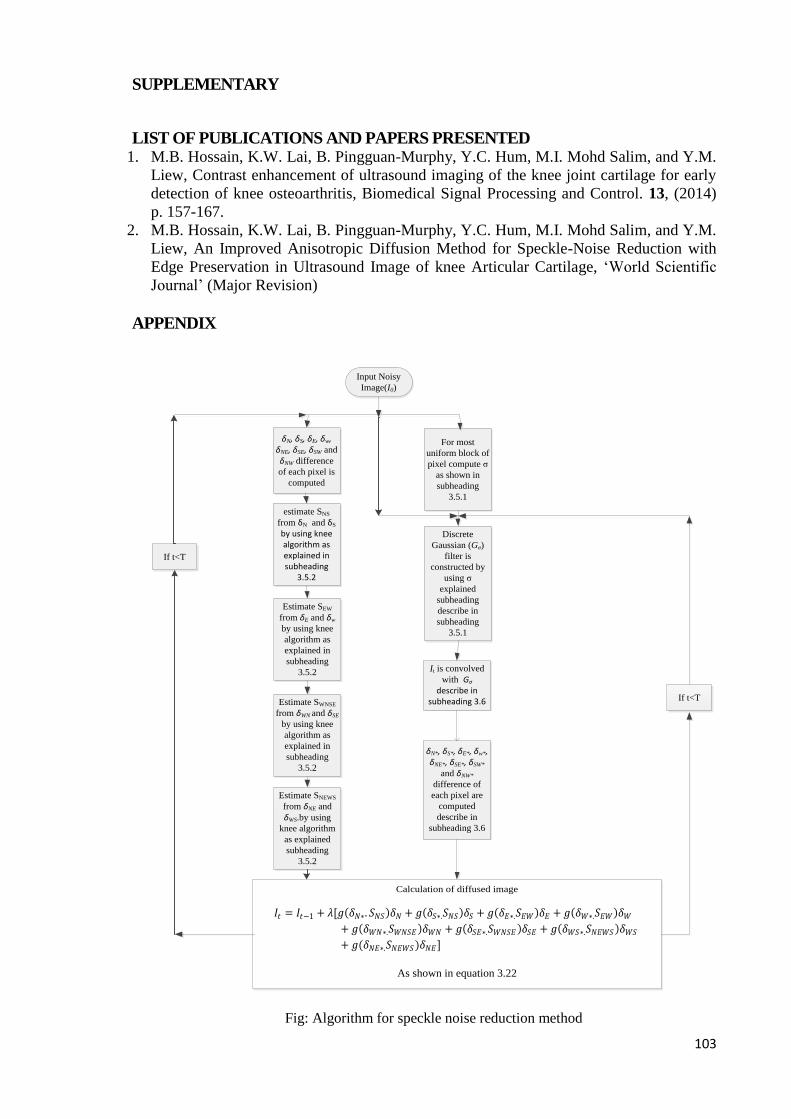
103
SUPPLEMENTARY
LIST OF PUBLICATIONS AND PAPERS PRESENTED 1. M.B. Hossain, K.W. Lai, B. Pingguan-Murphy, Y.C. Hum, M.I. Mohd Salim, and Y.M.
Liew, Contrast enhancement of ultrasound imaging of the knee joint cartilage for early
detection of knee osteoarthritis, Biomedical Signal Processing and Control. 13, (2014)
p. 157-167.
2. M.B. Hossain, K.W. Lai, B. Pingguan-Murphy, Y.C. Hum, M.I. Mohd Salim, and Y.M.
Liew, An Improved Anisotropic Diffusion Method for Speckle-Noise Reduction with
Edge Preservation in Ultrasound Image of knee Articular Cartilage, ‘World Scientific
Journal’ (Major Revision)
APPENDIX
Calculation of diffused image
Input Noisy
Image(I0)
δN, δS, δE, δw, δNE, δSE, δSW and
δNW difference
of each pixel is
computed
For most
uniform block of
pixel compute σ
as shown in
subheading
3.5.1
estimate SNS
from δN and δS
by using knee algorithm as explained in subheading
3.5.2
Discrete
Gaussian (Gσ)
filter is
constructed by
using σ
explained
subheading
describe in
subheading
3.5.1
It is convolved
with Gσ
describe in subheading 3.6
δN*, δS*, δE*, δw*, δNE*, δSE*, δSW*
and δNW*
difference of
each pixel are
computed
describe in
subheading 3.6
Estimate SEW
from δE and δw
by using knee
algorithm as
explained in
subheading
3.5.2
Estimate SWNSE
from δWN and δSE
by using knee
algorithm as
explained in
subheading
3.5.2
Estimate SNEWS
from δNE and
δWS.by using
knee algorithm
as explained
subheading
3.5.2
𝐼𝑡 = 𝐼𝑡−1 + 𝜆[𝑔(𝛿𝑁∗. 𝑆𝑁𝑆)𝛿𝑁 + 𝑔(𝛿𝑆∗.𝑆𝑁𝑆)𝛿𝑆 + 𝑔(𝛿𝐸∗.𝑆𝐸𝑊)𝛿𝐸 + 𝑔(𝛿𝑊∗.𝑆𝐸𝑊)𝛿𝑊
+ 𝑔(𝛿𝑊𝑁∗.𝑆𝑊𝑁𝑆𝐸 )𝛿𝑊𝑁 + 𝑔(𝛿𝑆𝐸∗.𝑆𝑊𝑁𝑆𝐸 )𝛿𝑆𝐸 + 𝑔(𝛿𝑊𝑆∗.𝑆𝑁𝐸𝑊𝑆 )𝛿𝑊𝑆
+ 𝑔(𝛿𝑁𝐸∗.𝑆𝑁𝐸𝑊𝑆 )𝛿𝑁𝐸]
As shown in equation 3.22
If t<T
If t<T
Fig: Algorithm for speckle noise reduction method

104
Input Image
Bi-histogram
equalization at
Xk
Output image
Input Image mean
compute as µx in
equation 3.1
Intensity
difference of
input image
mean and input
image pixel is
computed
Intensity
difference of
output image
mean and output
image pixel is
computed
Output image
mean is
computed µy in
equation 3.2
Standard
deviation of
input image
computed as
shown in
equation 3.7
Standard
deviation of
output image is
computed as
shown in
equation 3.8
ND computed
as in equation
3.13Normalized
brightness (NB)
is calculated as
shown in
equation 3.3
Normalized
contrast (NC)
has been
calculated as
shown in
equation 3.9
PBS is
computed with
specific α1, β1
parameter of
beta function as
in equation 3.4
PDS is
computed with
specific α3,β3
parameters of
beta function as
in equation 3.14
OCS is
computed with
specific α2, β2
function
parameter of
beta function as
in equation 3.10
NPBS computed as
in equation 3.6
NPDS computed as
in equation 3.15
NOCS Computed as
in equation 3.11
Final objective function
is constructed using
three objective functions
as shown in equation
3.16
Xk= Maximum
gray Level?
Search Xk that
maximize
objective
function output
in the stored
array
Yes
Store function
output in an
arrayK=k+1No
Fig: Algorithm for contrast enhancement method