Development of Transit Trip Time Model and Consolidation ... file2Professor, Transportation Engineering Group, Department of Civil Engineering & Associate Faculty CTRANS, IIT Roorkee,

European Transport \ Trasporti Europei (2016) Issue 61, Paper n° 3, ISSN 1825-3997

1

Development of Transit Trip Time Model and Consolidation of Bus Stops Based on Acceptable Walking Distance

Using GIS

Amita Johar1, S.S Jain2 and P.K Garg3

1Ph.D. Scholar, Centre for Transportation Systems (CTRANS), IIT Roorkee, Roorkee 247667, Uttarakhand, India,

[email protected] 2Professor, Transportation Engineering Group, Department of Civil Engineering & Associate Faculty CTRANS, IIT

Roorkee, Roorkee–247667, Uttarakhand, India,[email protected] 3Professor, Geomatics Engineering Group, Department of Civil Engineering & Associate Faculty CTRANS, IIT

Roorkee, Roorkee-247667, Uttarakhand, India,[email protected] Abstract Transit Trip Time is an important factor of transport system because it affects the efficiency of system and service attractiveness. If a

transit trip time is appropriate it attracts more commuters and increases the commuters’ satisfaction.

The objective of this study is to develop a regression model that provides better understanding of factors that affects the total trip

time on the route. After the development of regression model, the bus stops on the selected routes were consolidated based on

mean/acceptable walking distance using ArcGIS software. The study was conducted on two selected urban bus routes of Delhi

Transport Corporation (DTC). Field data collected includes arrivals/departure times, delays, average speed and distance between the

bus stops, walking distance of the commuter from bus stop to their destination, age, sex, type of employment, purpose of trip, mode

of travel, walking travel time and income of commuter. For development of regression model, dwell time, delays and distance

between the bus stops was taken as input data. Developed model was validated and tested using GPS (Global Positioning Data)

collected from field study. Finally, the results indicate that consolidation of bus stops could improve the travel time and save total

travel time cost.

Keywords: Regression Model, Urban Route, Transit Trip Time, ArcGIS.

1. Introduction

In metropolitan cities like Delhi, life of urban dwellers depends on an efficient transport

system. Even after the beginning of metro, the major commuters depend on bus transport for convenient and comfortable movement within the city (Master Plan of Delhi, 2021). The reliability of bus service is a key factor in influencing the choice of public transport (Lesely, 1976). The main

Corresponding author: Amita Johar ([email protected])


2

factor to be considered for efficient transport system is transit trip time because it affects the efficiency and reliability of the system. Transit trip time is an indicator that describes the performance of the system for use in day to day operation management for planning and scheduling of route process (Bertini and El-Geneidy, 2004). Transit trip time is an essential component of transport system as it attracts more commuters and increases the commuter’s satisfaction. The objective of this study is to develop a trip time model for better understanding of the parameters that influence the transit trip time and help traveller in making their trip decision for better performance assessment. After the development of trip time model the bus stops on the selected routes were consolidated based on mean/acceptable walking distance using ArcGIS software. The model values were revealed using data collected for selected urban bus route.

2. Research Survey

In most of the previous studies, development of trip time model and optimize spacing of bus stops were done independently to avoid computational burden. Most of the researchers developed transit trip time regression model. Some of them are discussed below: Regression model estimates the values of dependent variables from the values of independent variables. Regression model can work under unstable traffic condition. Advantage of regression models is that they tell which inputs are less or more important for predicting travel time. Abdelfattah and Khan (1998) build a linear and nonlinear regression model to predict bus delay using simulation data. The model was used to predict bus delay under normal condition, when one traffic lane is blocked. It meets the calibration test and was confirmed by field data. You and Kim (2000) developed a hybrid model for predicting travel time for the road network that is congested. To implement the hybrid model, the core forecasting algorithm with non-parametric regression technique has been integrated in GIS technology. Based on the results, it is indentified that hybrid model can be used for various ITS application. Zhang and Rice (2003) build an efficient and easily-implementable model to predict freeway travel time using linear regression analysis. The effectiveness of the method is tested using two loop detector data sets. Mean absolute prediction percentage error (MAPPE) was used to check the prediction accuracy. Results state that method is acceptable for many transportation applications. Patnaik et al. (2004) build a regression model to calculate arrival time of the bus and also identify the problem that occurred during processing of data collected through APC (automatic passenger counting) units. Automatic passenger counters placed on the buses was used to collect the data. The data was collected from January to June 2002. The model was used to calculate arrival time of bus under various conditions. The proposed model estimated bus arrival times under various situations. Ramakrishna et al. (2007) build a MLR (multi linear regression) model to predict bus travel time using GPS probe data and passenger data. The route no 21 G from Tambaram to Parrys in the city of Chennai, having 19 bus stops and about 32 Km in length is chosen as a case study. It is indentified from the data analysis that similar traffic condition exists over the route during the peak hour on all weekdays. One of the limitations of this model is that it should be recalibrated before applying on other urban routes. Chang et al. (2010) developed a dynamic model based on Nearest Neighbour Non-parametric Regression. The model was developed to estimate path travel times between origin and destination bus stops. The Automatic vehicle technology was used to collect the real world data. The proposed model was tested and the results indicate that developed model performed effectively in terms of accuracy and computational time. Yu et al. (2014) developed a model using SVM (support vector machine) regression method to predict travel time of bus. Once the data was collected, the Grubb;s test was applied to remove the errors among the collected samples. To assign power to the recent data,


3

forgetting factor was introduced. Based on the result it is identified that SVMFFG (SVMS with forgetting factor and Grubb’s test) method outperforms than other three methods, i.e., SVMs, SVMG (SVMS with Grubb’s test) and SVMFF (SVMs with forgetting factor). Most of the researchers optimize spacing between bus stops. Some of them are discussed below: The important part to deal with transit service planning process is to identify the appropriate location and spacing of bus stop. The quality of the transit service in terms of bus travel time and budgetary resources of transit provider can be improved by appropriate spacing of bus stop (Wirasinghe and Ghoneim, (1981); Fitzpatrick et al., (1997); Kuah and Perl, (1988); Chien and Qin, (2004); Ziari et al., (2007)). Most of the researchers optimize bus stop spacing using GIS (Furth et al., (2007); Xuebin, (2010); Huang and Liu, (2014)). Some of them are discussed below: El-Shair (2003) determines optimal spacing of bus stops using GIS in the Birkenhead region of Auckland, New Zealand. He stated that if 80 % or more of the residential area and commercial areas are located within a buffer zone of 300 m from all bus stops then sufficiency of bus stop/bus routes in the region can be achieved. Sankar et al. (2003) discussed the optimization of bus stop location using GIS and GPS. A multi-criteria analysis was performed taking into consideration all the parameters, like density of population, minimum and maximum distance between two successive bus stops, willingness to walk, detail of junction point and monetary status of people. For optimal location of bus stop a maximum distance of not more than 2 km and minimum distance of 500 m was set. The software used for analysis, digitization and transformation projection was Arc View and Arc Info (GIS software). GIS was used to analyze all the criteria and derive good results. Adebola and Enosko (2012) developed a GIS-based methodology to identify best location of bus stops and to enhance public transport system in Ibadan North, Oyo State. Bus stops were determined using three basic attributes i.e., stop location, stop spacing and evaluation of characteristics. Methodology developed accomplished the principles of good access which are safety, affordability, accessibility and reliability. Biba et al. (2010) developed a parcel network method that estimates the population within walking distance to transit facilities and network distance from parcel to transit facilities. In this method, the integration of cadastral data with network analysis holds promise for research in many areas of GIS. The results of network parcel method were derived and compared with buffer and network ratio methods. Shretha and Zolnik (2013) stated that travel time and operating cost can be reduced by eliminating bus stop. They also stated that elimination of bus stops is good for environment because it reduce annual CHGs emission of CO (carbon monoxide), VOCs (Volatile Organic Compound) and NOx (Nitrogen Oxide) by 6,278, 241 and 1,789 lbs, respectively. Limitation of this study is that they did not consider the tradeoff of lost ridership due to elimination of most accessible bus stop and adverse effect on commercial, residential and shopping trips due to elimination of bus stop. Revathy and Lakshmi (2013) used GIS and remote sensing stop based coverage ratio index method to find out the pedestrian network to bus stop, and thereby identifying served and un-served areas by public transport services. Stop coverage Ratio Index was obtained as

Ideal Stop-Accessibility Index (ISAI) can be used to evaluate the accessibility to a bus stop through surrounding pedestrian road network. It is obtained as

Actual Stop-Accessibility Index (ISAI) can be used as a more accurate measure of bus stop accessibility through the surrounding pedestrian road network. It is obtained as


4

Madhan and Lakshmi (2013) discussed a conceptual approach using GIS for rationalization of bus stops using various parameters, like passenger density, land use pattern nearness to generating points, bus stop capacity and spacing between stops for its effective location and utilization. The capacity of bus stop can be calculated as

Where, Bbb= bus stop capacity (bus/h); g/c = green time ratio ; tc =clearance time(s) td = average dwell time Za= standard normal variables corresponding to a desired failure rate Cv = coefficient of variation of dwell time. Huang (2014) described a general framework using GIS to optimize the distribution of bus stop. In this study, three levels of bus stops were defined; firstly connection stop were generated. Secondly, key stop were generated using coverage model in order to minimize the average weight distance, and lastly, stops were optimized with coverage model to maximize custom coverage ordinary. Results show improvement on service area by reducing redundant stops in central area, and some bus stops are deployed to outer area.

3. Data Collection and Basic Statistics

Data was collected for two urban bus routes i.e. 832 and 817 in Delhi, India to develop regression model. The detail of both the routes are shown in Table 1.The urban bus route 832 runs from Janakpuri D Block to Inderlock Metro Station via Sagarpur, Tilak Nagar, Moti Nagar and Inderlock while route number 817 runs from Kair Village to Inderlock Metro Station via kair Depot, TudaMandi, KakrolaMor, Janakpuri East Bus Stop, Tilak Nagar, Inderlock as shown in Figure 1. Table 1: Detail of Urban Bus Route Number 832 and 817

S. No Detail of Bus Route Name of Urban Bus Route

Route No. 832 Route No.817

1. Length 14 (Km) 28( km)

2. Travel Time 60-80 Minutes 100-120 minutes

3. Number of Bus Stops 33 53

4. Number of Intersection 16 20


5

Figure 1: Layout of Urban Bus Route No. 832 and 817 in Delhi

Data has been collected through site visit for the duration of 5 weekdays in the month of February, 2014. Location for collecting the data was inside the bus for all the stops situated along the bus routes. The data was collected separately for each route. For this study parameters were collected using handled GPS (Global Positioning System). Data collected include arrival time/departure times, delays, average speed between the bus stops and distance between the stops. Dwell time at each stop was calculated using arrival time and departure time at each stop. The arrival time is recorded as the bus arrive the stop circle, and departure time is recorded as bus leaves the stop circle. The arrival time and departure time are recorded for all the stops even if bus does not stop to serve the passengers. Dwell time is defined as the sum of total time the door remains open and alighting and boarding of passengers take place and door closes. The correlation among the variables has been shown in the Table 2. From Table 2 we found that speed is correlated with distance (0.55) and delay (0.597) and hence it was dropped. Therefore, the input variables considered to develop the regression model were dwell time, delays and distance between the stops. Table 2 : Correlation of Variables

Variable Dwell Time Distance Delay Speed

Dwell Time 1

Distance 0.1813837 1

Delay -0.023431 -0.16655 1

Speed 0.0428633 0.553016 0.597309925 1

Consolidation of bus stops was another objective which is done on the basis of mean/acceptable walking distance. To calculate the mean/acceptable walking distance data was through physical survey conducted in the month of March 2014, at various bus stops along the selected urban bus routes. The survey was done in the morning from 7:00 am to 11:00 am and in the


6

evening from 4:00 pm to 7:00 pm. Trips included during the survey were work, shopping, education and recreational trips. A total of 2000 samples were obtained out of which 1748 samples were used for analysis. The information related to commuters at the bus stops was obtained by requesting the respondents to indicate the walking distance from origin to destination, age, sex, type of employment, purpose of trip, mode of travel, walking travel time and income of commuter. Exploratory Data Analysis (EDA) was done to describe the basic characteristics of parameters of trip time model and outcomes from the analysis are given in Table 3 and Table 4.

Table 3: Results from EDA Analysis on Parameters of Trip Time Model for Route Number 832

Statistics of

Data

832 (upstream) 832 (Downstream)

Dwell Time (Seconds) Delay

(Seconds)

Distance

(meters) Dwell Time (Seconds)

Delay

(Seconds)

Distance

(meters)

Minimum 0 0 28.24 0 0 113.45

Maximum 50.0 180.00 753.92 48.00 466.00 834.93

Mean 11.875 28.740 418.707 11.945 48.789 424.136

Std. Deviation 8.151 31.841 174.056 8.941 57.210 189.893

Variance 66.454 1013.887 30295.782 79.942 3273.028 36059.491

Table 4 : Results from EDA Analysis on Parameters of Trip Time Model for Route Number 817

Statistics of

Data

817 (upstream) 817 (Downstream)

Dwell Time (Seconds) Delay

(Seconds)

Distance

(meters) Dwell Time (Seconds)

Delay

(Seconds)

Distance

(meters)

Minimum 0 0 181.10 0 0 115.28

Maximum 50.00 655.00 1854.27 48.00 1400.00 1929.83

Mean 10.769 48.052 522.908 11.113 58.296 546.411

Std.Deviation 8.666 63.907 290.178 9.053 93.944 312.315

Variance 75.116 4084.113 84203.584 81.973 8825.558 97540.682

4. Proposed Trip Time Model

A set of data records considered for analysis of model is as shown in Table 5.Multiple

regression analysis was performed to develop a transit trip time prediction model. The independent variables used in the model include distance between the stops, delays (at intersection and due to congestion) and dwell time at stops. The dependent variable used is Travel Time (TT in seconds). In regression analysis the total data set has been divided in the two parts that is training and testing in the ratio 75 and 25 percent respectively. After the model is developed 25 percent data was used to test the developed model. The finally calibrated model is as shown in Eq. 5.


7

TT= a + b*Distance +c*Delay + d*Dwell Time (5) Where, a, b, c, d are constants. Table 5: Data Records Considered for Analysis of Models

S.No Models Name Data used for Development of Models Set of Data Records

1. Model I 832 (upstream) 512

2. Model II 832 (downstream) 512

3. Model III 832(Combined upstream and downstream) 1024

4. Model IV 817(upstream) 832

5. Model V 817(downstream) 800

6. Model VI 817(Combined upstream and downstream) 1632

The six regression models were calibrated and have been illustrated in the Table 6.

Table 6 : Calibration of Six Regression Model

Model Equation R2

Model I TT=24.13+1.15(dwell)+1.09(delay)+0.10(distance) 0.81

Model II TT=19.69+1.14(dwell)+1.33(delay)+0.06(distance) 0.89

Model III TT=21.63+1.15(dwell)+1.35(delay)+0.07(distance) 0.79

Model IV TT=15.64+1.17(dwell)+1.49(dwell)+0.04(distance) 0.84

Model V TT=9.67+1.09(dwell)+1.37(dwell)+0.06(distance) 0.87

Model IV TT=11.18+1.17(dwell)+1.45(dwell)+0.05(distance) 0.83

5. Model Performance

After the development of model it is necessary to estimate the performance in terms of accuracy and robustness. Figure 2 and Figure 3 show the comparison between the actual and predicted trip time of six models for testing phase. The Actual and predicted trip time was compared to check the validity of the models. Figure 4 and Figure 5 show the scatter plots of models for testing phase. To check the performance of the developed model three measure of effectiveness were used that is RMSE (Root Mean square Error), MAPE (Mean Absolute Percentage Error) and R2 (coefficient of correlation). RMSE is defined as the difference between the predicted and actual travel time. MAPE is defined as the average difference between the predicted and actual travel time. MAPE and RMSE have been defined as shown in the Eq. 6 and 7.

(6)

(7)

Where, y1 is the predicted values of transit travel time


8

y0 is actual values of transit travel time. n is the number of data point in the set

Figure 2: Actual and Predicted Tip Time for Testing Phase of Route Number 832 (a) Model I (b) Model II (c) Model III

(a) (b)

(c)


9

Figure 3: Actual and Predicted Trip Time Testing Phase of Route Number 817

(a) Model IV (b) Model V(c) Model VI

(a) (b)

(c)


10

Figure 4: Scatter Plot between Actual and Predicted for Testing Phase of Route Number 832

(a) Model I (b) Model II (c) Model III

(a) (b)

(c)


11

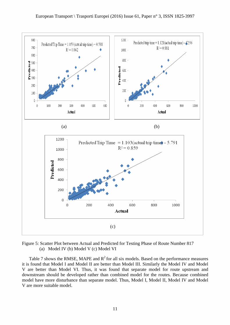
Figure 5: Scatter Plot between Actual and Predicted for Testing Phase of Route Number 817

(a) Model IV (b) Model V (c) Model VI

Table 7 shows the RMSE, MAPE and R2 for all six models. Based on the performance measures it is found that Model I and Model II are better than Model III. Similarly the Model IV and Model V are better than Model VI. Thus, it was found that separate model for route upstream and downstream should be developed rather than combined model for the routes. Because combined model have more disturbance than separate model. Thus, Model I, Model II, Model IV and Model V are more suitable model.

(a)

(c)

(b)


12

Table 7 : Summary of Output of Six Models for Testing Phase

6. Consolidation of Bus Stops Using GIS

After the proposed model has been develop, it is necessary to observe the impact of input parameters on the cost of providing transit service. The length of the route number 832 and 817 is 14 km and 28 Km approximately without any average distance between the stops. In general there is contradiction between providing too many stops (that increases the accessibility and result in larger trip time) and less number of stops (that decreases the accessibility and result in lesser trip time). It is a complex task to optimize the location of transit stops, but stops can be moved or consolidated due to shift in demographic and development changes. Consolidation stops is one of the basic approach that decreases the trip time and improve the quality of bus service (Wirasinghe and Ghoneim, 1981; Saka, 2001; Alterkawi, 2006). The quality of bus service can be improved by proper spacing of stops. To determine proper spacing of the bus stops one should have better understanding of how far people are willing to walk to get to the facility (Ziari et al., 2007). If consolidation of bus stops is done on mean/acceptable walking distance then it will eliminate total of 10 stops from route number 832 and 7 stops from route number 817 and will result in decrease trip time.

7. Eliminating Bus Stops

After evaluating the selected urban route, it was identified that spacing between the bus stops was un-equal. Some bus stops are closely located resulting in waste of time & space, and some bus stops are sparsely located resulting in longer walking distance (Adebola and Enosko, 2012). If we consider the consolidation of stops on mean/acceptable walking distance that is 647 m (Johar et. al. 2015), then it will eliminate some stops from the route and also result in decrease travel time of the trip. Thus the choice of the commuters to use the transit service increases if the transit stop are provided within a reasonable walking distance of one’s origin and destination (Gahlot et al., 2013). In this study consolidation of bus stop using GIS involves following steps:

1. Digitizing the urban route as line feature and bus stops as point feature from Google Earth. 2. Digitized point and line feature are then converted from KML to layer. 3. The data is then converted to appropriate coordinate system. 4. The consolidation of bus stop is done on mean/acceptable walking distance that is 647

meters. 5. The 647 meters interval was arrived at by digitizing the urban route as lines feature in such a

way that all the vertices are within 647 meters. The line features were then converted to point features and the point features were automatically spaced at 647 meters interval.

6. Bus stop coverage area is the area within the defined distance from bus stop. The half length of mean walking distance that is 324 meters is used to define the bus stop coverage area.

Models Name R2 RMSE MAPE

Model I 0.812 18.427 16.234

Model II 0.889 23.51 18.940

Model III 0.801 27.257 21.324

Model IV 0.862 34.750 25.193

Model V 0.881 46.692 22.054

Model VI 0.859 47.366 28.972


13

Figure 6 shows the bus stops placed at distance of 647 meters and each bus stop covering an area within 324 meters of bus stops. From the Figure 6 it is identified that large amount of area does not fall under the influencing zone and the commuters staying in the area which does not fall under the influencing zone have to walk longer than the 324 m. Therefore, in order to include large amount of area under the influencing zone, the distance between two bus stops must be reduced to about 580 m. Finally, if the bus stops are placed at a distance of 580 m and each bus stop covering an area within 324 m of bus stop. Then the large amount of area fall under the influencing zone, and commuters staying in the area have to walk approximately equal to 324 m as shown in Figure 7. This strategy is used to place the bus stops as the metro stations are placed in Delhi. This will improve the efficiency of bus service by eliminating stops which will decrease travel time. Table 8 summarizes the stop changes on Route no 832 and 817. The decrease in travel time is calculated in next section. The decrease in travel time is calculated in next section

Table 8: Summary of Stops Changes on Route No. 832 and 817

Route Direction Stop Before/After Stops Removed Average Spacing Before/After

832 Upstream 33/23 10 Unequal/580 meters

817 Downstream 53/46 7 Unequal/580 meters

Figure 6: Urban Bus Route showing Area not under Influencing Zone


14

Figure 7 : Urban Bus Route with Circular Buffer Zone around Proposed Stop and Area under the

Influencing zone was reduced

8. Total Travel Time Cost

Travel time is defined as the cost of time spent on transport, including waiting as well as actual travel time. Therefore, the value of travel time saved due to saving travel time has a considerable share in transport cost (Kumar, 2014). The total travel time costs are the product of time spent in travelling multiplied by the unit cost (Small et al., 2005).

Saving of Travel Time Approximately 10 stops were eliminated from route number 832 and 7 stops were eliminated from route number 817 based on mean/acceptable walking distance between the scheduled bus stops to 580 m and bus stop covering an area of 324 m. According to the proposed model it was identified that that on an average one stop utilizes 12.23 seconds and after consolidation of bus stop on the basis of mean/acceptable walking distance 10 stops from route number 832 and 7 stops from route number 817 was reduced. Therefore, total trip time of both the routes would be reduced to approximately 122.3 seconds (2.038 min) and 85.61seconds (1.43 min). DTC operates 12 buses per day from Janakpuri D Block to Inderlock Metro Station and each bus travel 7 trips per day. Therefore, total trips per day would be 84 trips (12 buses/day * 7 trips). So, during 12-h period the total time saved due to elimination of stops would be 171.192 minutes (84 trips/day * 2.038 min) per day. This results in ability to add two additional trips to the selected route.


15

Similarly, DTC operates 12 buses per day from KairVillage to Inderlock Metro Station and each bus travel 6 trips per day. Therefore, total trips per day would be 72 trips (12 buses/day * 6 trips). So, during 12-h period the total time saved due to elimination of stops would be 102.96 minutes (72 trips/day * 1.43 min) per day. This results in ability to add one additional trip to the selected route. Total 16 trips per direction were collected to developed and validate trip time model for the selected the selected urban bus route. Therefore, on an average total passenger boarded the bus per trip was 214 passengers. So, the total saving of time per trip for route number 832 would be 36635.088 (84 trips *2.038 minutes* 214 passengers). Similarly, the total saving of time per trip for route number 832 would be 22033.44 (72 trips *1.43 minutes* 214 passengers).

Value of Travel Time

Value of Travel Time (VOT) plays a crucial role in the cost benefits analysis in transport planning. It quantifies the importance of time with respect to cost which is employed in economic evaluation of travel time saving (Minal, 2014). To calculate the average value of time per minute, the monthly income for various commuters has been collected from the interview survey conducted in the month of March 2014. Total 5 working days were considered in a week. Therefore, the total working days in a year is 261 days (365 days in a year- 104 Saturday and Sunday). The hourly wage rate is calculate by considering 8 working hour per day, hourly wage rate for 261 days is 2088 hours (261working days * 8 working hour per day). To calculate the annual income, the average monthly income is then multiplied by 12 months. Hourly wage rate is calculated by dividing the annual income by total number of working hours that is 2088 hours. This hourly wage rate is again divided by 60 minutes to get average value of time per minute.

Mean monthly income = INR 21117.34 Annual income = INR 253408.16 Hourly wage rate = INR 121.36 per hour Average value of time = INR 2.18 per min The average value of time thus obtained is 2.18 INR /min.

Total Travel Time Cost

The total travel time costs saved are the product of total saving of time per minutes multiplied by the average value of time (VOT). Travel Time Cost = saving of time* VOT (8) The total travel time cost saved is INR 79864 for route number 832 and INR 48032 for route number 817.

9. Conclusion

Transit trip time is an important parameters for public transport system as it attracts the commuters and increase commuters satisfaction. In this study, the trip time model for two selected urban bus routes in Delhi was developed from the data collected through field visits. The performance of the developed model is evaluated using coefficient of correlation (R2), root mean square error (RMSE), mean absolute percentage error (MAPE). Based on the performance measure it is revealed that Model I, Model II, Model IV and Model V are more suitable model.


16

After development of trip time model consolidation of bus stops was done based on mean/acceptable walking distance. The mean/acceptable walking distance of commuters from different categories in Delhi according to lognormal distribution curve is 647 m. Consolidation of bus stop based on mean/acceptable walking distance eliminated 10 stops from route number 832 and 7 stops from route number 817. Elimination of bus stop results in saving of travel time and total travel time cost. The total travel time and travel cost saved is 36635.088 minutes and INR 79864 for route number 832 and total travel time and travel cost saved is 22033.44 minutes and INR 48032 for route number 817. For further work, it is suggested that proposed model can be improved by in cooperating the information of schedule adherence. It is also suggested to evaluate bus related emission such as CO (carbon monoxide), VOCs (Volatile organic Compunds) and NOx (Nitrogen Oxide). References

Abdelfattah, A.M., Khan, A.M. (1998) “Models for Predicting Bus Delays”, Transportation

Research Record 1623 (1), pp. 8-15.

Adebola, O. and Enosko, O. (2012) “Analysis of Bus-Stops Location Using Geographic

Information System In Ibadan North L.G.A Nigeria”, IISTE 2 (3), pp. 20-37.

Alterkawi, M. (2006) “A computer simulation analysis for optimizing bus stops spacing: The case

of Riyadh, Saudi Arabia”, Habitat International 30 (3), pp. 500-508.

Bertini, R. L. and EI-Geneidy, A. M. (2004) “Modeling Transit Trip Time Using Archived Bus

Dispatch System Data”, Journal of Transportation Engineering 130 (1), pp. 56-67.

Biba, S., Curtin, K.M. and Manca, G. (2010) “A New Method for Determining the Population with

Walking Access to Transit”, International Journal of Geographic Information Science 24 (3),

pp. 347-364.

Chang, H., Park, D., Lee, S., Lee, H. and Baek, S. (2010) “Dynamic Multi-Interval Bus Travel

Time Prediction Using Bus Transit Data”, Transportmetrica, 6(1), pp.19-38.

Chien, S. l., and Qin, Z. (2004) “Optimization of Bus Stop Locations for Improving Transit

Accessibility”, Transportation Planning and Technology 27 (3), pp. 211-227.

El-Shair, I. M. (2003) “GIS and Remote Sensing in Urban Transportation Planning: A Case Study

of Birkenhead, Auckland”, Map India Conference.

Fitzpatrick, K., Perkinson, D., and Hall K. (1997) “Findings from a Survey on Bus Stop Design”.

Journal of Public Transportation 1 (3), pp. 17-27.

Furth, P. G., Mekuria, M. C. and San Clemente, J.L. (2007) “Stop Spacing Analysis using

Geographic Information System Tools with Parcel and Street Network Data”, Transportation

Research Record, Journal of Transportation Research Board, Washington, D.C, 2034, pp.73-

81.


17

Gahlot, V., Swami, B. L., Parida, M. and Kalla, P. (2013) “Availability and Accessibility

Assessment of Public Transit System in Jaipur City”, International Journal of Transportation

Engineering 1 (2), pp. 81-91.

Huang, Z. (2014) “A Hierarchical Process for Optimizing Bus Stop Distribution”, Urban Planning

and Transport Research: An Open Access Journal 2 (1), pp. 162-172.

Huang, Z. and Liu, X. (2014) “A Hierarchical Process for Optimizing Bus Stop Distribution in

Large and Fast Developing Countries” ISPRS International Journal of Geo-Information, 3, pp.

554-564.

Johar, A., Jain, S.S., Garg, P.K., and Gundaliya, P.J. (2015) “A Study of Commuter Walk Distance

From Bus Stops to Differnt Destination along Routes in Delhi’, Traspoti Europei 59 (3).

Kuah, G. K. and Perl, J. (1988) “Optimization of Feeder Bus Routes and Bus-Stop Spacing”,

Journal of Transportation Engineering 114 (3), pp. 341-354.

Kumar, P. (2014) Urbanization in Asia. Springer

Lesley L.J.S (1976) “Optimum Bus Stop Spacing”, Traffic Engineering and Control 17(10), pp.

399-401.

Madhan, A. and Lakshmi, S. (2013) “Rationalization of Bus Stop Using GIS-A Conceptual

Approach”, Journal of Road Transport 9, pp. 36-45.

Master plane of Delhi (2021). See www.dda.org.in/planning/draft_master_plans.htm . Access on

24/12/2013

Minal (2014) Mode Choice Analysis using Neuro-Fuzzy Model, Mtech Thesis, CSIR-Central Road

Research Institute.

Patnaik, J., Chien, S., and. Bladikas, A. (2004) “Estimation of Bus Arrival Times Using APC

Data”, Journal of Public Transportation 7 (1), pp. 1-20.

Ramakrishna, Y., P. Ramakrishna, V. Lakshmanan, and R. Sivanandan. (2006) “Bus travel time

prediction using GPS Data”, In Proceedings of Map India. Access on

February 2014 from <http://www.gisdevelopment.net/proceedings/mapindia/2006/>

Revathy, P. and Lakshmi, S. (2013) “Identifying the Un-Served Areas through Application of

GIS” Journal of Road Transport 9, pp. 29-35.

Saka, A. A. (2001) “Model for Determining Optimum Bus-Stop Spacing in Urban Areas”, Journal

of Transportation Engineering 127(30), pp. 195-199.

Sankar R., Kavitha, J. and Karthi, S. (2003) “Optimization of Bus Stop Locations using GIS as a

Tool for Chennai City—A Case Study”, Map India Conference, Poster session.


18

Shretha, R. M. and Zolnik, E. J. (2013) “Eliminating Bus Stops: Evaluating Changes in

Operations, Emissions and Coverage”, Journal of Public Transportation 16 (2), pp. 153-175.

Small, K., Winston, C. and Yan, J. (2005) “Uncovering the Distribution of Motorists’ Preferences

for Travel Time and Reliability: Implications for Road Pricing”, University of Irvine.

Wirasinghe, S. and Ghoneim, N. S. (1981) “Spacing of Bus-stops For Many-to-Many Travel

Demand”, Transportation Research Record 15 (3), pp. 210-221.

Xuebin, W. (2010) Optimizing Bus stop Location in Wuhan, China, Ph.D Thesis, International

Institute for Geo-Information Science and Earth Observation Enschede, The Netherlands.

You, J. and Kim, T. J. (2000) “Development and Evaluation of Hybrid Travel Time Forecasting

Model”, Transportation Research Part C 8, pp. 231-256.

Yu, B., Ye, T., Tian, X.-M. , Ning, G.-B., and Zhong, S.-Q. (2014) “Bus Travel Time Prediction

with Forgetting Factor”. Journal of Computing in Civil Engineering ASCE, pp. 06014002-1 to

06014002-6.

Zhang, X. and Rice, J. A. (2003) “Short-Term Travel Time Prediction Using A Time-Varying

Coefficient Linear Model”, Transportation Research Part C 11, pp. 187-210.

Ziari, H., Keymanesh, M. and Khabiri, M. (2007) “Locating Stations of Public Transportation

Vehicles for Improving Transit Accessibility”, Transport 22 (2), pp. 99-104.

Acknowledgements

The Financial support in the form of MHRD fellowship from Indian Institute of Technology

Roorkee, India, to Ms Amita Johar is gratefully acknowledged

Documents

Development of Transit Trip Time Model and Consolidation ... file2Professor, Transportation Engineering Group, Department of Civil Engineering & Associate Faculty CTRANS, IIT Roorkee,