Development of the Next Generation Stratified Ramp Metering Algorithm Based on Freeway Design

Final Report

Prepared by:

Nikolas Geroliminis Anupam Srivastava

Panos Michalopoulos

Department of Civil Engineering University of Minnesota

CTS 11-05

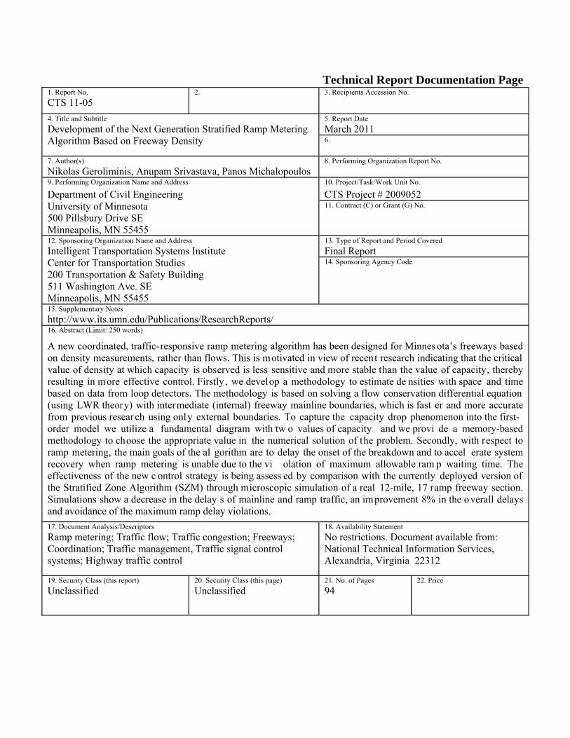
Technical Report Documentation Page 1. Report No. 2. 3. Recipients Accession No. CTS 11-05 4. Title and Subtitle 5. Report DateDevelopment of the Next Generation Stratified Ramp Metering Algorithm Based on Freeway Density

March 2011 6.

7. Author(s) 8. Performing Organization Report No. Nikolas Geroliminis, Anupam Srivastava, Panos Michalopoulos 9. Performing Organization Name and Address 10. Project/Task/Work Unit No. Department of Civil Engineering University of Minnesota 500 Pillsbury Drive SE Minneapolis, MN 55455

CTS Project # 2009052 11. Contract (C) or Grant (G) No.

12. Sponsoring Organization Name and Address 13. Type of Report and Period Covered Intelligent Transportation Systems Institute Center for Transportation Studies 200 Transportation & Safety Building 511 Washington Ave. SE Minneapolis, MN 55455

Final Report 14. Sponsoring Agency Code

15. Supplementary Notes http://www.its.umn.edu/Publications/ResearchReports/ 16. Abstract (Limit: 250 words)

A new coordinated, traffic-responsive ramp metering algorithm has been designed for Minnes ota’s freeways based on density measurements, rather than flows. This is motivated in view of recent research indicating that the critical value of density at which capacity is observed is less sensitive and more stable than the value of capacity, thereby resulting in more effective control. Firstly , we develop a methodology to estimate de nsities with space and time based on data from loop detectors. The methodology is based on solving a flow conservation differential equation (using LWR theory) with intermediate (internal) freeway mainline boundaries, which is fast er and more accurate from previous research using only external boundaries. To capture the capacity drop phenomenon into the first-order model we utilize a fundamental diagram with tw o values of capacity and we provi de a memory-based methodology to choose the appropriate value in the numerical solution of the problem. Secondly, with respect to ramp metering, the main goals of the al gorithm are to delay the onset of the breakdown and to accel erate system recovery when ramp metering is unable due to the vi olation of maximum allowable ram p waiting time. The effectiveness of the new c ontrol strategy is being assess ed by comparison with the currently deployed version of the Stratified Zone Algorithm (SZM) through microscopic simulation of a real 12-mile, 17 ramp freeway section. Simulations show a decrease in the delay s of mainline and ramp traffic, an improvement 8% in the overall delays and avoidance of the maximum ramp delay violations.

17. Document Analysis/Descriptors Ramp metering; Traffic flow; Traffic congestion; Freeways; Coordination; Traffic management, Traffic signal control systems; Highway traffic control

18. Availability Statement No restrictions. Document available from: National Technical Information Services, Alexandria, Virginia 22312

19. Security Class (this report) 20. Security Class (this page) 21. No. of Pages 22. Price Unclassified Unclassified 94

Development of the Next Generation Stratified Ramp Metering Algorithm Based on Freeway Density 

Final Report

Prepared by:

Nikolas Geroliminis Anupam Srivastava

Panos Michalopoulos

Department of Civil Engineering University of Minnesota

March 2011

Published by:

Intelligent Transportation Systems Institute Center for Transportation Studies

200 Transportation & Safety Building 511 Washington Avenue SE

Minneapolis, Minnesota 55455

The contents of this report reflect the views of the authors, who are responsible for the facts and the accuracy of the information presented herein. This document is disseminated under the sponsorship of the Department of Transportation University Transportation Centers Program, in the interest of information exchange. The U.S. Government assumes no liability for the contents or use thereof. This report does not necessarily reflect the official views or policies of the University of Minnesota. The authors, the University of Minnesota, and the U.S. Government do not endorse products or manufacturers. Any trade or manufacturers’ names that may appear herein do so solely because they are con sidered essential to this report.

ACKNOWLEDGEMENTS

The authors wish to acknowledge those who made this research possible. The study was funded by the Intelligent Transportation Systems (ITS) Institute, a program of the University of Minnesota’s Center for Transportation Studies (CTS). Financial support was provided by the United States Department of Transportation’s Research and Innovative Technologies Administration (RITA). The authors also acknowledge Brian Kary and Doug Lau of Minnesota Department of Transportation’s Regional Traffic Management Center (RTMC) and Dr. John Hourdos of the University of Minnesota, for their valuable comments, support, and continuous cooperation.

CONTENTS Chapter 1 Introduction ............................................................................................................................... 1

Chapter 2 Empirical Observations at Bottlenecks ................................................................................... 5

Bottlenecks and Capacity Drop .................................................................................................................... 5

Observations at Bottlenecks .......................................................................................................................... 7

Study Site and Data Analysis ........................................................................................................................ 7

Capacity Drop Observations ......................................................................................................................... 8

Phase Diagrams ........................................................................................................................................... 12

Chapter 3 Density Profile Modeling ........................................................................................................ 21

Density Modeling ........................................................................................................................................ 21

Extended First-Order Modeling .................................................................................................................. 23

Simulation Results ...................................................................................................................................... 28

Conclusions ................................................................................................................................................. 40

Chapter 4 Ramp Metering and Observations ........................................................................................ 41

Ramp Metering in Minnesota ..................................................................................................................... 42

Stratified Zone Metering Algorithm ........................................................................................................... 43

Observations about SZM ............................................................................................................................ 47

Chapter 5 New Ramp Metering ............................................................................................................... 51

Proposed Algorithm .................................................................................................................................... 51

Associated Variables and Parameters ......................................................................................................... 53

Bottleneck and Zone Identification ............................................................................................................. 55

Action Matrix .............................................................................................................................................. 58

Application and Results .............................................................................................................................. 61

Test Site and Input Data .............................................................................................................................. 61

AIMSUN API ............................................................................................................................................. 62

Chapter 6 Results and Analysis ............................................................................................................... 67

Results and Comparisons ............................................................................................................................ 67

Conclusions ................................................................................................................................................. 71

References .................................................................................................................................................. 73

Appendix A: New Ramp Metering Algorithm

Appendix B: Map of Test Site (US169-NB)

LIST OF FIGURES Figure 2-1: Graphs showing relationships between traffic state parameters ................................................ 6

Figure 2-2: The selected test site – US169 Northbound ............................................................................... 8

Figure 2-3: Time series plot of throughput at bottleneck (5 min averages) .................................................. 9

Figure 2-4: Oblique plot of cumulative throughput at bottleneck ............................................................... 10

Figure 2-5: Fundamental diagram plot between flow and density at bottleneck ........................................ 11

Figure 2-6: Phase diagram and demand at ramp, September 17, 2008 ....................................................... 14

Figure 2-7: Phase diagram and demand at ramp, September 10, 2008 ....................................................... 15

Figure 2-8: Phase diagram, September 25, 2001 ........................................................................................ 16

Figure 2-9: Phase diagram, November 15, 2000 ........................................................................................ 16

Figure 2-10: Time series of throughput and ramp discharge rate at bottleneck .......................................... 18

Figure 3-1: Simulation obtained density vs. linear approximation model .................................................. 22

Figure 3-2: Application of the LWR model to a section of the freeway ..................................................... 24

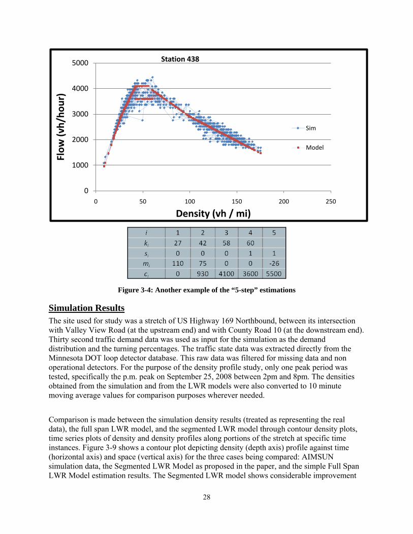
Figure 3-3: Model “5-step” stepwise linear flow - density relation ............................................................ 27

Figure 3-4: Another example of the “5-step” estimations .......................................................................... 28

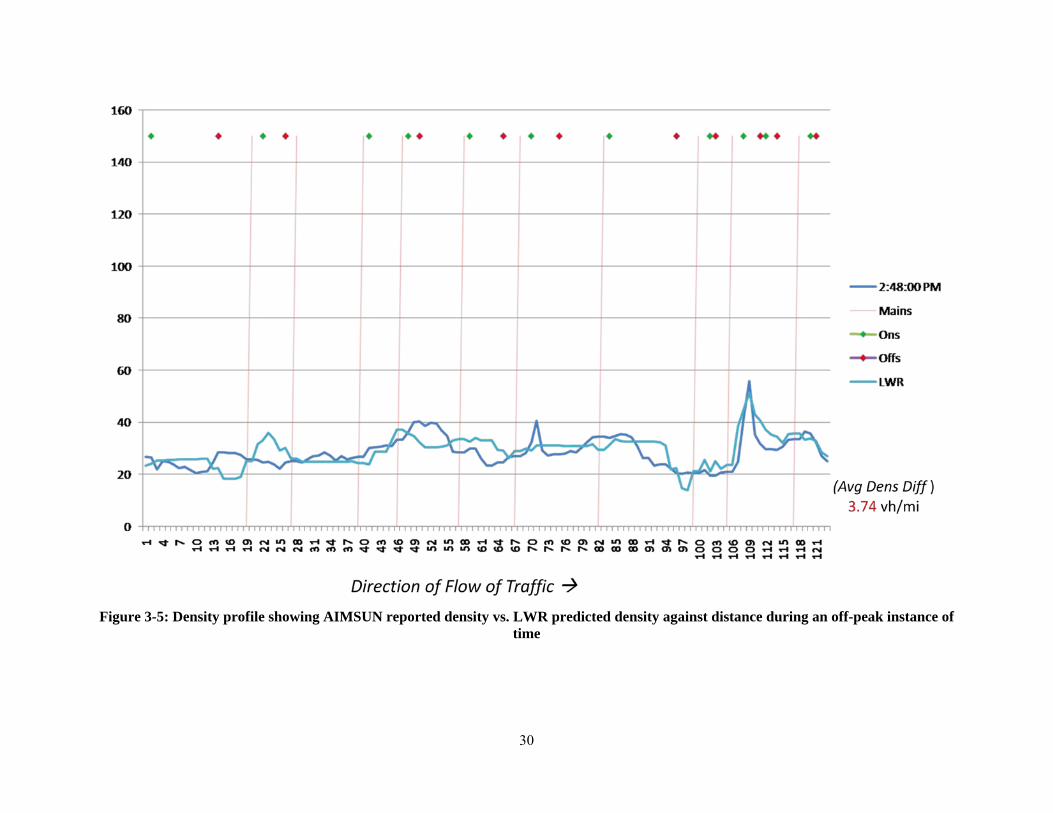
Figure 3-5: Density profile showing AIMSUN reported density vs. LWR predicted density against distance during an off-peak instance of time .............................................................................................. 30

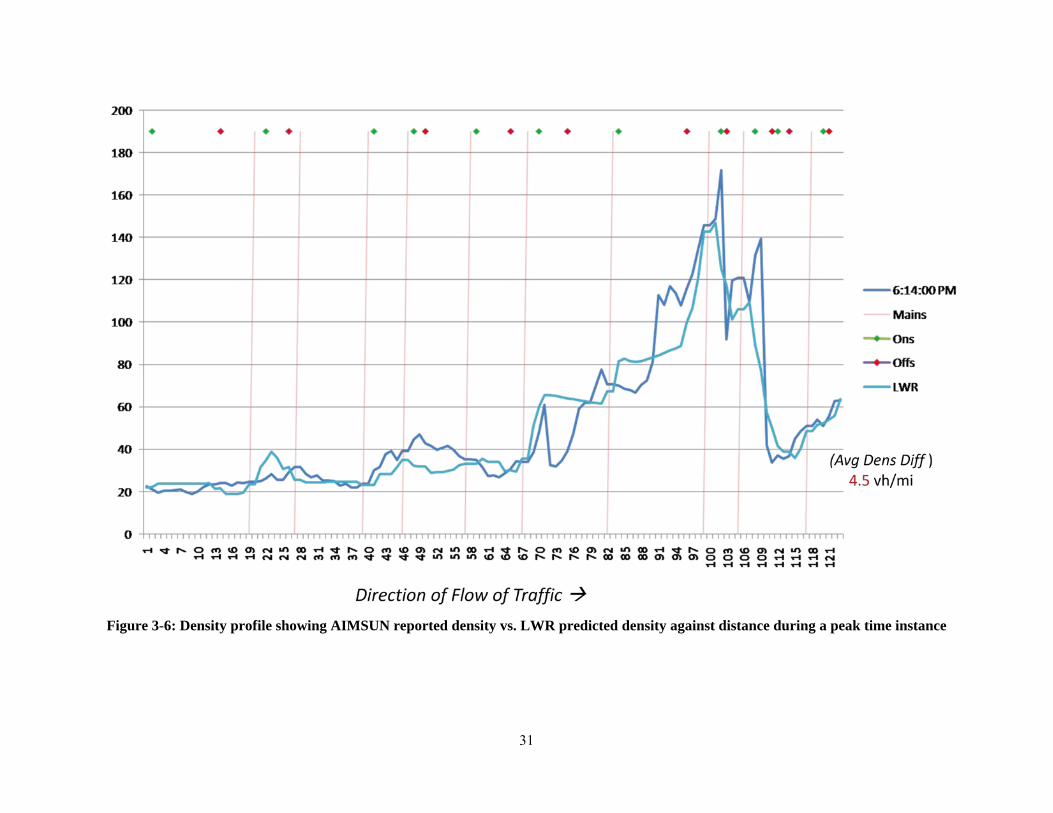
Figure 3-6: Density profile showing AIMSUN reported density vs. LWR predicted density against distance during a peak time instance ........................................................................................................... 31

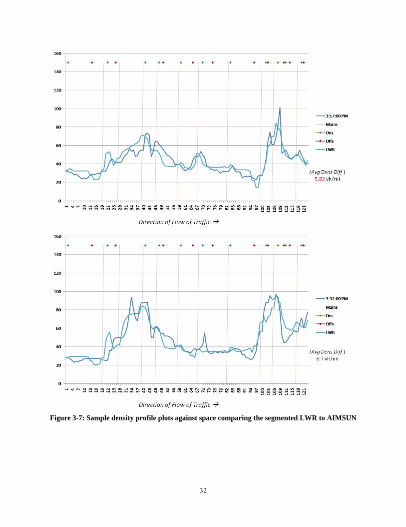
Figure 3-7: Sample density profile plots against space comparing the segmented LWR to AIMSUN ...... 32

Figure 3-8: Sample density profile plots against space comparing the segmented LWR to AIMSUN ...... 33

Figure 3-9: Density contour plots comparing AIMSUN vs. traditional LWR vs. segmented LWR .......... 34

Figure 3-10: Binary density contour plots (threshold = 50vh/mi) for AIMSUN vs. segmented LWR vs. full length LWR model ............................................................................................................................... 35

Figure 3-11: Binary density contour plots (threshold = 30vh/mi) for AIMSUN vs. segmented LWR vs. full length LWR model ............................................................................................................................... 36

Figure 3-12: Time series plot of density at Cedar Lake ramp location showing a comparison of AIMSUN vs. segmented LWR vs. traditional LWR ................................................................................................... 38

Figure 3-13: Time series plot of density at Excelsior Blvd. ramp to US 169 NB comparing AIMSUN to Segmented LWR and traditional LWR model estimations ......................................................................... 39

Figure 4-1: Stratified zone definition example for SZM (source: [27]) ...................................................... 45

Figure 4-2: Structure of the Stratified Zone Metering algorithm (source: [27]) ......................................... 46

Figure 4-3: Queue size time series plot against ramp wait-times at 3 upstream on-ramps ......................... 48

Figure 4-4: Ramp metering rates time series plot for an active bottleneck location ................................... 49

Figure 5-1: A figurative summary depicting zone identification ................................................................ 57

Figure 5-2: Assignment of control strategies following zone identification ............................................... 59

Figure 5-3: On ramp demands for the study site ......................................................................................... 62

Figure 5-4: Schema of AIMSUN API module and process of information exchange ................................ 64

Figure 5-5: AIMSUN and AIMSUN API module interaction scheme ....................................................... 65

LIST OF TABLES Table 6-1: Network MOEs for SZM and new metering (Sep 25, 2008, 2:00pm-8:00pm) ......................... 68

Table 6-2: Ramp MOEs during peak period (Sep 25, 2008, 4:00pm-6:30pm) ........................................... 68

Table 6-3: MOEs observed for various values of T for all ramps along network ...................................... 69

Table 6-4: MOEs observed for various values of T for TH62 ramp .......................................................... 70

EXECUTIVE SUMMARY

This project is a natural next stage of earlier successfully completed projects for improving Minnesota Department of Transportation’s (Mn/DOT) stratified ramp metering strategy. Based on Mn/DOT Regional Traffic Management Center (RTMC)’s recommendation, we explore alternatives for developing the next generation strategy to address limitations and substantially enhance the performance of the currently deployed Stratified Ramp Metering strategy. Following a different approach, we develop the Next Generation strategy by focusing on density rather than flow. This is because (as shown in earlier research) while values of near-capacity occupancy are quite stable, bottleneck capacity has stochastic variations, and thus a control strategy based on flow thresholds is likely to be inefficient. This variability in the capacity flow would mean that a control strategy based on flow thresholds would be likely to either under-load the freeway during the uncongested regime of traffic flow, or overload the system after the occurrence of the breakdown. While the former might lead to early onsets of congestion (congestion not being delayed as much as possible since the full capacity of the system is not utilized), the later might mean that the system is unable to recover from congestion efficiently (due to an over-load on the system). Critical occupancy however, and therefore density, is known to have stable behavior at capacity. This suggests that using a density based control approach can potentially enhance the overall performance of the system. During the first part of the project we developed a methodology to estimate densities with space and time based on data from loop detectors. The methodology is based on solving a flow conservation differential equation (using LWR theory) with intermediate (internal) freeway mainline boundaries, which is faster and more accurate than previous research using only external boundaries. Capacity drop phenomenon is inherently incorporated in the density estimation process, and the effect of the stochastic nature of capacity flow is minimized by identifying bottleneck threats and zones based on critical density values. Results compared with micro-simulation of a long freeway stretch show that this model produces reliable and accurate results. We further extended this density estimator using a two-value capacity (before and after the occurrence of a breakdown) and we integrated it in the LWR formulation. By carefully analyzing empirical data of active bottlenecks in the Twin Cities Metropolitan Area we noticed that (i) there are many cases where capacity is underutilized (4 min ramp delay constraint is misinterpreted by the algorithm) and (ii) the system once congested is unable to return to a state of flow near capacity for too long. One of the main reasons for the above inefficiencies is that capacity is considered constant during all times at all bottlenecks. This is concluded based on two empirical findings: (i) a significant capacity drop after the breakdown in many locations (varying 0-15%) and (ii) the total capacity of a bottleneck (sum of mainline + on ramp) is a function of the ratio of the two flows. More specifically, when ramp flows are higher the capacity is smaller (~5-10%). This happens very often in Minnesota ramps because of the 4 minute constraint in ramp delays. Instead of a layer-based algorithm, we proceed with a dynamic zone-based algorithm. The whole freeway system is divided into zones, where the length of each zone is dynamic and is estimated

in real-time. Within each zone the metering rates are chosen independently of conditions in other zones. The algorithm’s goal is to keep the car density levels at all ramps below the congestion thresholds and not to allow low speeds to occur in the mainline, by constraining the ramp delays. The ramp rates become stricter when mainline density is close to the congestion threshold, and the ramp rates increase when ramp waiting times are close to the ramp delay threshold. When it is not possible to keep both uncongested because of high on-ramp and mainline demands, the algorithm seeks to delay as long as possible the violation of both thresholds. The effectiveness of the new control strategies has been assessed by comparison with the current stratified zone metering (SZM) version through microscopic simulation for the H-169 site. Under the new control strategy the total travel time on the mainline decreased by 1.5%, the ramp total travel time dropped by nearly 20%, the total system (freeway and ramp) travel time decreased by about 3% and total delays decreased by 8%. This finding suggests that in this case the new strategy is very effective since it reduces not only ramp delay, but also total system delay. The results clearly indicate that the new control strategy is very effective in keeping ramp wait times below the maximum allowed and in reducing ramp delay time. Another interesting observation made by analyzing the simulation results is that the new strategy substantially reduces ramp queues, while the overall ramp delay for the peak period was reduced by nearly 30%. The effectiveness of the newly developed control strategy is then assessed using the AIMSUN traffic micro-simulator against the currently deployed strategy. The new metering strategies is deployed on a simulated network and implemented using the AIMSUN API module. The strategy is compared against the current strategy using various measures of effectiveness and is found to succeed in delaying the onset of breakdown, accelerating system recovery after breakdown, and improving the overall freeway and ramp performances (through improved speeds and throughputs and reduced delays and stoppages). A proposal for field implementation of the new strategy and of comparison studies of performance based on ‘before’ and ‘after’ studies is suggested as a follow up for the study.

1

Chapter 1 INTRODUCTION

Ramp control has been recognized as an effective strategy of increasing freeway operation efficiency. It has been reported that ramp metering was able to reduce delay by 101 million person hours in 2002, 5% of the congestion delay on freeways with ramp metering. Ramp metering is the application of control devices such as metering signals to limit the number of vehicles entering a freeway. Over the years, a number of ramp control strategies have been developed in order to regulate the entrance ramp demand to freeways. It is one of the most efficient tools to mitigate congestion, other than adding more capacity to transportation infrastructures. The fundamental philosophy of ramp metering is that a corridor can maintain its optimal operation by regulating the freeway demand to be under its capacity. Over the years, a number of traffic-responsive ramp control strategies have been developed in order to regulate the entrance ramp demand to freeways. These strategies use basic principles of feedback and feed-forward controls with minor modifications and can be classified as isolated or coordinated.

The main objectives of ramp metering strategies are:

1. To maintain free-flow traffic conditions in all sections of a freeway for as long as possible, while minimizing the occurrence of onramp queue spillbacks from on-ramps to arterial roads,

2. When congestion occurs, minimize its negative effect on freeway throughput and return freeway conditions to free-flow state as fast as possible, and

3. To optimize freeway throughput while employing equitable ramp metering policies for all travelers.

Ramp metering has a long history in traffic management. As reported by Bogenberger and May (1999) [2] various forms of ramp metering were used experimentally in Detroit, New York, and St. Louis in the early 1960's. In Chicago, traffic responsive ramp meters have been in operation on the Eisenhower Expressway since 1963. Eight ramp meters were installed on the Gulf Freeway in Houston in 1965 and operated successfully until freeway reconstruction caused their removal in 1975. Over 30 ramp meters were operated successfully on the North Central Expressway in Dallas from 1971 until major freeway reconstruction forced most of them to be removed in 1990. In Los Angeles, ramp metering began 1968. The system has been expanded continually until there are now about 1300 meters in operation in metropolitan Los Angeles, making it the largest system in the world. Coordinated traffic responsive control was first implemented in the 1970's and is gradually spreading to many freeway control systems both in the United States and abroad. Ramp meters are currently operating in more than 20 metropolitan areas in the United States and also in many other parts of the world, like Australia, Holland, Japan, Germany, Sweden, Denmark etc.

In the Twin Cities metropolitan area, the first implementation of freeway ramp metering started in 1969, when the Minnesota Department of Transportation tested ramp metering in I-35E. According to Regional Transportation Management Center the system has grown to include 419 ramp meters - of which 213 meters have the potential to operate during the morning peak and 266 meters have the potential to operate in the evening peak. Prior to year 2000, the deployed

2

control strategy, i.e., the ZONE Metering strategy (Lau, 1996), focused on maximizing freeway capacity utilization without handling ramp queue spillbacks in arterial streets and controlling ramp waiting times. While breakdowns at freeway bottlenecks were effectively prevented with the ZONE algorithm, ramp delays and queues were often excessive (Hourdakis and Michalopoulos, 2002 [15]). The latter resulted in public complains, leading to a six-week system-wide shutdown study in late 2000. A study by Cambridge Systematics (2001) [4] confirmed the overall benefits of the ZONE strategy, but it also “highlighted the need for modifications towards an efficient but more equitable ramp control algorithm.” Mn/DOT developed a new one aiming to strike a balance between freeway efficiency and reduced ramp delays. This new strategy, termed stratified zone metering (SZM), takes into accounts not only freeway conditions but also real time ramp demand and queue size information (Xin et al., 2004 [41]). Implementation of the new strategy with the Twin Cities freeway system began in early 2002; full deployment was completed in 2003. Michalopoulos et al (2005) [27] compared the effectiveness of the new SZM strategy with the ZONE algorithm and the No Control case using extensive micro-simulation in two test sites. Their evaluation results indicate that the Stratified Zone Metering Strategy meets its objective of controlling ramp queue spillbacks and reducing ramp delay; also it is still beneficial as compared to the No Control alternative in terms of improving freeway performance and safety. However, this is accomplished at the expense of freeway and system performance as expected. The evaluation suggested that the SZM showed 50%-80% decrease in ramp delays on tested sites, accompanied with up to 70% reduction in total travel time on ramps, when compared to ZONE metering. Though the freeway delays increased from those seen with ZONE, they were still lower (reduced by 8%-14%) than the No-Control scenario. In this report, we first analyze empirical data from loop detectors in the Twin Cities Metropolitan and we develop insights about the performance of the algorithms and the involved traffic phenomena. The existing Stratified Ramp metering algorithm from Mn/DOT calculates the total metering rates per zone by balancing total input flow and output flow for a section and keeps flows under the threshold capacity levels. The stochastic variations known to exist in this threshold capacity value however, limit the usability and efficiency of such a metering strategy. The variability in capacity would mean that a flow dependent control strategy is likely to either under-load the freeway during the free flow phase, or overload the system after breakdown in the congested regime. Whereas past ramp metering studies done in Minnesota have always considered flow-based approaches to ramp metering, this study explores the feasibility of control strategies that focus on densities. The project also incorporates the positive aspects of a coordinated control strategy while still serving the restraint requirement on the maximum allowable ramp wait times, which is a required additional constraint for Minnesota’s freeway system. Previous analysis of real traffic data from freeway merge areas in different locations has indicated that the recurrent traffic breakdown during peak hours can occur at different flow values, even under the same weather and lighting conditions [9]. Also, probabilistic characteristics of capacity have been observed broadly in the literature (e.g. Kuhne and Mahnke [18], Brilon [3]) due to breakdown phenomena or variability of weather conditions. But since capacity is random (between certain values) a control strategy based on flow thresholds is likely to under-load the freeway or lead to traffic congestion. On the other hand, various researches

3

indicate that the critical value of occupancy at which capacity is observed is less sensitive and quite stable. Therefore, it is desirable to develop a new methodology to overcome this randomness to make the Stratified Ramp Control strategy more robust and more adaptive to the freeway geometry and real time traffic conditions. The new strategy, which is presented here, overcomes traditional problems of existing strategies that i) cannot reliably estimate freeway storage capacity, ii) are not efficient at realizing the full capacity of the freeway and thus cannot efficiently postpone onset of mainline congestion, and iii) are not efficient at recovering from an existing congestion condition since they tend to overload the congested system. The new strategy is aimed at improving upon the existing control strategy without compromising the equity based maximum allowable ramp delay constraint. The remainder of the report is divided into 5 main chapters. Chapter 2 presents findings from analysis of freeway bottleneck behavior of traffic. In this chapter we explore the existence of the capacity drop phenomenon, and attempt to analyze the effects of ramp metering strategies on the capacity drops observed. This is followed in the third chapter with a proposal of a methodology to estimate density profiles accurately along the stretch of a freeway using available loop detector data. The density estimation model develops upon the existing LWR modeling technique and also employs a memory based decision system to account for the effects of the capacity drop phenomenon. Chapter 4 gives an introduction to the currently deployed Stratified Zone Metering strategy and identifies aspects of the strategy that can be improved upon. We present the new metering strategy in the 5th chapter, which is developed based on the findings from the previous portions of the study. The proposed strategy is a density based coordinated control strategy that implements real time identification of bottleneck threats and zones of influence to decide metering rates for on-ramps. In the final chapter, we compare the effectiveness of the proposed strategy against the existing SZM strategy using AIMSUN simulation.

4

5

Chapter 2 EMPIRICAL OBSERVATIONS AT BOTTLENECKS

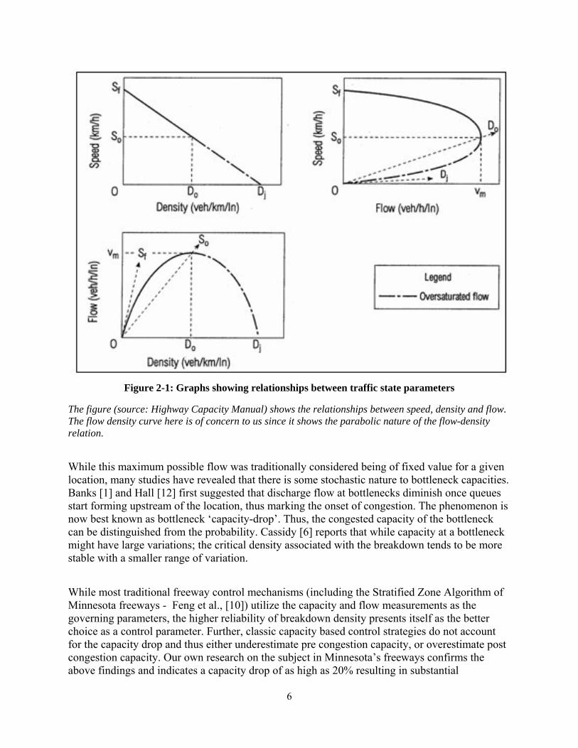
Bottlenecks and Capacity Drop While the original expectation from freeways was to allow uninterrupted freely flowing traffic at all times with maximum level of service, they are known to often become congested in recent times. Congestions on road networks are caused due to the formation of bottlenecks. A bottleneck is a phenomenon where the full performance level (capacity) of an entire system cannot be realized due to an abnormality at a single component of the system. The performance at one location thus brings down the performance of the entire system. An ‘active’ bottleneck is a bottleneck whose performance is not affected by any bottlenecks occurring downstream, and has free-flow conditions downstream. The traffic flow through a section of a freeway is the measure of rate of movement of traffic through a section, either defined per lane, or for the entire width of the section. Traffic flow is known to have a near parabolic relation with traffic density, as explained by Greenshields (shown in Figure 2-1). Under free-flow conditions, while density is low, flow rises with increasing density as speed does not get affected. However, as density increases, flow peaks and then starts to drop as the freeway section enters a state of congestion. The capacity at a bottleneck can be defined as the maximum throughput possible at the bottleneck or the maximum net traffic flow exiting the bottleneck. Similarly, the capacity of freeway network sections is most commonly defined as the maximum flow possible at the bottleneck under the current circumstances. Many later studies analyzing data from different sites have identified an asymmetric fundamental diagram, where the critical density (value which maximizes flow), is lower than half of the jam density.

6

Figure 2-1: Graphs showing relationships between traffic state parameters

The figure (source: Highway Capacity Manual) shows the relationships between speed, density and flow. The flow density curve here is of concern to us since it shows the parabolic nature of the flow-density relation. While this maximum possible flow was traditionally considered being of fixed value for a given location, many studies have revealed that there is some stochastic nature to bottleneck capacities. Banks [1] and Hall [12] first suggested that discharge flow at bottlenecks diminish once queues start forming upstream of the location, thus marking the onset of congestion. The phenomenon is now best known as bottleneck ‘capacity-drop’. Thus, the congested capacity of the bottleneck can be distinguished from the probability. Cassidy [6] reports that while capacity at a bottleneck might have large variations; the critical density associated with the breakdown tends to be more stable with a smaller range of variation. While most traditional freeway control mechanisms (including the Stratified Zone Algorithm of Minnesota freeways - Feng et al., [10]) utilize the capacity and flow measurements as the governing parameters, the higher reliability of breakdown density presents itself as the better choice as a control parameter. Further, classic capacity based control strategies do not account for the capacity drop and thus either underestimate pre congestion capacity, or overestimate post congestion capacity. Our own research on the subject in Minnesota’s freeways confirms the above findings and indicates a capacity drop of as high as 20% resulting in substantial

7

miscalculation of the optimal metering rates. This suggests that a control strategy based on flow thresholds is likely to under-load the freeway or lead to traffic congestion.

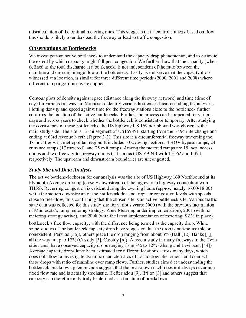
Observations at Bottlenecks We investigate an active bottleneck to understand the capacity drop phenomenon, and to estimate the extent by which capacity might fall post congestion. We further show that the capacity (when defined as the total discharge at a bottleneck) is not independent of the ratio between the mainline and on-ramp merge flow at the bottleneck. Lastly, we observe that the capacity drop witnessed at a location, is similar for three different time periods (2000, 2001 and 2008) where different ramp algorithms were applied. Contour plots of density against space (distance along the freeway network) and time (time of day) for various freeways in Minnesota identify various bottleneck locations along the network. Plotting density and speed against time for the freeway stations close to the bottleneck further confirms the location of the active bottlenecks. Further, the process can be repeated for various days and across years to check whether the bottleneck is consistent or temporary. After studying the consistency of these bottlenecks, the US highway US 169 northbound was chosen as the main study side. The site is 12-mi segment of US169-NB starting from the I-494 interchange and ending at 63rd Avenue North (Figure 2-2). This site is a circumferential freeway traversing the Twin Cities west metropolitan region. It includes 10 weaving sections, 4 HOV bypass ramps, 24 entrance ramps (17 metered), and 25 exit ramps. Among the metered ramps are 15 local access ramps and two freeway-to-freeway ramps that connect US169-NB with TH-62 and I-394, respectively. The upstream and downstream boundaries are uncongested.

Study Site and Data Analysis The active bottleneck chosen for our analysis was the site of US Highway 169 Northbound at its Plymouth Avenue on-ramp (closely downstream of the highway to highway connection with TH55). Recurring congestion is evident during the evening hours (approximately 16:00-18:00) while the station downstream of the bottleneck does not register congestion levels with speeds close to free-flow, thus confirming that the chosen site is an active bottleneck site. Various traffic state data was collected for this study site for various years: 2000 (with the previous incarnation of Minnesota’s ramp metering strategy: Zone Metering under implementation), 2001 (with no metering strategy active), and 2008 (with the latest implementation of metering: SZM in place). bottleneck’s free flow capacity, with the difference being termed as the capacity drop. While some studies of the bottleneck capacity drop have suggested that the drop is non-noticeable or nonexistent (Persuad [36]), others place the drop ranging from about 3% (Hall [12], Banks [1]) all the way to up to 12% (Cassidy [5], Cassidy [6]). A recent study in many freeways in the Twin cities area, have observed capacity drops ranging from 3% to 12% (Zhang and Levinson, [44]). Average capacity drops have been estimated for different locations across many days, which does not allow to investigate dynamic characteristics of traffic flow phenomena and connect these drops with ratio of mainline over ramp flows. Further, studies aimed at understanding the bottleneck breakdown phenomenon suggest that the breakdown itself does not always occur at a fixed flow rate and is actually stochastic. Elefteriadou [9], Brilon [3] and others suggest that capacity can therefore only truly be defined as a function of breakdown

8

Figure 2-2: The selected test site – US169 Northbound

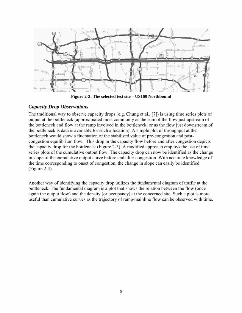
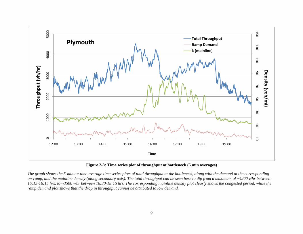
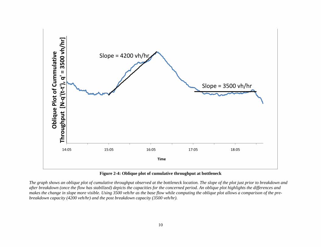
Capacity Drop Observations The traditional way to observe capacity drops (e.g. Chung et al., [7]) is using time series plots of output at the bottleneck (approximated most commonly as the sum of the flow just upstream of the bottleneck and flow at the ramp involved in the bottleneck, or as the flow just downstream of the bottleneck is data is available for such a location). A simple plot of throughput at the bottleneck would show a fluctuation of the stabilized value of pre-congestion and post-congestion equilibrium flow. This drop in the capacity flow before and after congestion depicts the capacity drop for the bottleneck (Figure 2-3). A modified approach employs the use of time series plots of the cumulative output flow. The capacity drop can now be identified as the change in slope of the cumulative output curve before and after congestion. With accurate knowledge of the time corresponding to onset of congestion, the change in slope can easily be identified (Figure 2-4). Another way of identifying the capacity drop utilizes the fundamental diagram of traffic at the bottleneck. The fundamental diagram is a plot that shows the relation between the flow (once again the output flow) and the density (or occupancy) at the concerned site. Such a plot is more useful than cumulative curves as the trajectory of ramp/mainline flow can be observed with time.

9

-1010

3050

7090

110130

1500

1000

2000

3000

4000

5000

12:00 13:00 14:00 15:00 16:00 17:00 18:00 19:00

Density (veh/m

i)Th

roug

hput

(vh/

hr)

Time

PlymouthTotal Throughput

Ramp Demand

k (mainline)

Figure 2-3: Time series plot of throughput at bottleneck (5 min averages)

The graph shows the 5-minute-time-average time series plots of total throughput at the bottleneck, along with the demand at the corresponding on-ramp, and the mainline density (along secondary axis). The total throughput can be seen here to dip from a maximum of ~4200 v/hr between 15:15-16:15 hrs, to ~3500 v/hr between 16:30-18:15 hrs. The corresponding mainline density plot clearly shows the congested period, while the ramp demand plot shows that the drop in throughput cannot be attributed to low demand.

10

14:05 15:05 16:05 17:05 18:05

Obl

ique

Plo

t of C

umm

ulat

ive

Thro

ughp

ut [

N-q

'(t-t

'), q

' = 3

500

vh/h

r]

Time

Slope = 3500 vh/hr

Slope = 4200 vh/hr

Figure 2-4: Oblique plot of cumulative throughput at bottleneck

The graph shows an oblique plot of cumulative throughput observed at the bottleneck location. The slope of the plot just prior to breakdown and after breakdown (once the flow has stabilized) depicts the capacities for the concerned period. An oblique plot highlights the differences and makes the change in slope more visible. Using 3500 veh/hr as the base flow while computing the oblique plot allows a comparison of the pre-breakdown capacity (4200 veh/hr) and the post breakdown capacity (3500 veh/hr).

11

010

0020

0030

0040

0050

00

0 10 20 30 40 50 60 70 80 90

Tota

l Thr

ough

put

(vh/

hr)

Density Mainline (vh/mi/lane)

PlymouthFundamental Diagram

Figure 2-5: Fundamental diagram plot between flow and density at bottleneck

The fundamental diagram for the US169 NB - Plymouth bottleneck location (based on 5 minute time average values) shows a similar ‘gap’ incapacity from ~4200 v/hr during free flow conditions to ~3500 v/hr post congestion The total throughput (sum of mainline and ramp flows) is compared against density at the mainline. Thus the plot is an approximate of conditions immediately upstream of the bottleneck location.

12

We present a representative throughput time series plot (sum of volumes at the upstream mainline detector station and volumes at the on ramp merge) in Figure 2-3, which shows a capacity drop of roughly 16.5% (from ~4200vh/hr pre congestion between around 16:15 to ~3500vh/hr during congestion as seen after 16:30). Speed profiles have significantly higher values before the occurrence of the breakdown, at 16:20. The figure also shows the ramp demand separately in the same plot so as to provide an estimate of the demand at the bottleneck. Note that ramp flow significantly increases a few minutes before the breakdown, while similar total demand at 16:05 did not create a breakdown because on-ramp flow was lower. The Flow versus Density plot for the bottleneck (using flow as the total output flow at the bottleneck as defined earlier, and density at the upstream mainline detector), shown in Figure 2-5 also shows the 16.5% capacity drop (from a peak at ~4200 during the uncongested regime to ~ 3500 during congestion). The density values used here and henceforth in the report are obtained directly from Mn/DOT’s data tools and repositories and are a simple transformation of recorded occupancies (using an average vehicle length of 22feet). High values of densities are observed because the location of the detector is slightly upstream of the merge location. This plot is useful to understand the value of capacity before and after the occurrence of the breakdown. Downstream conditions are always uncongested (smaller density and speed close to free flow). We further show in the following portion of the paper that these capacity drop values also remain constant across a vast time horizon (2000 – 2008) and under varying ramp control mechanisms.

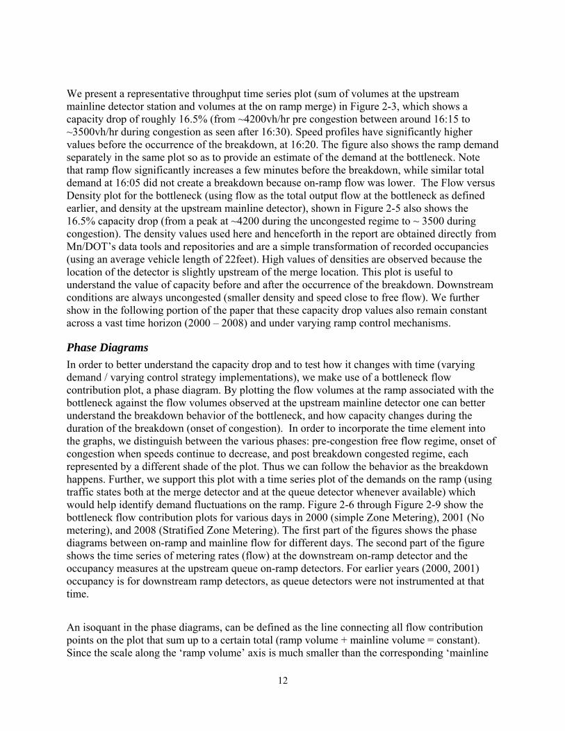
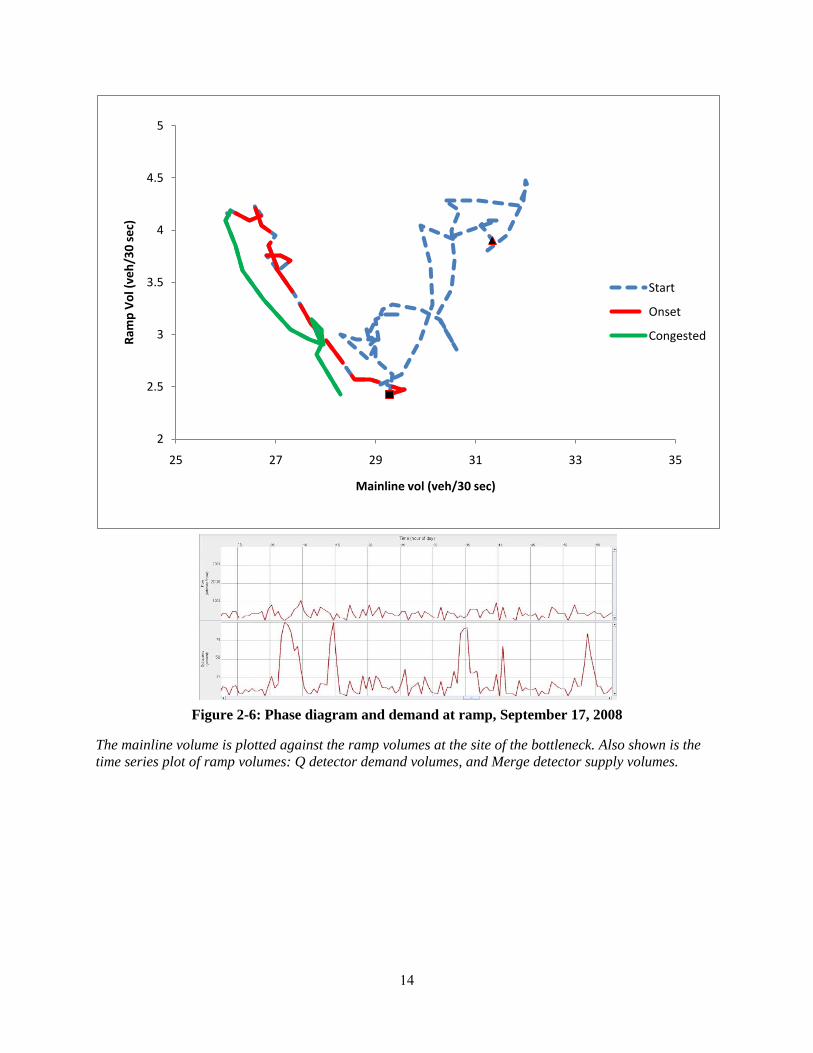
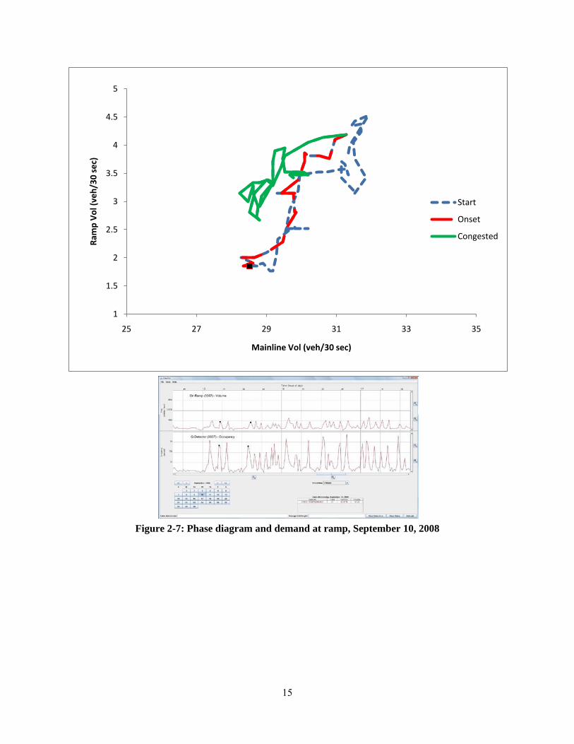
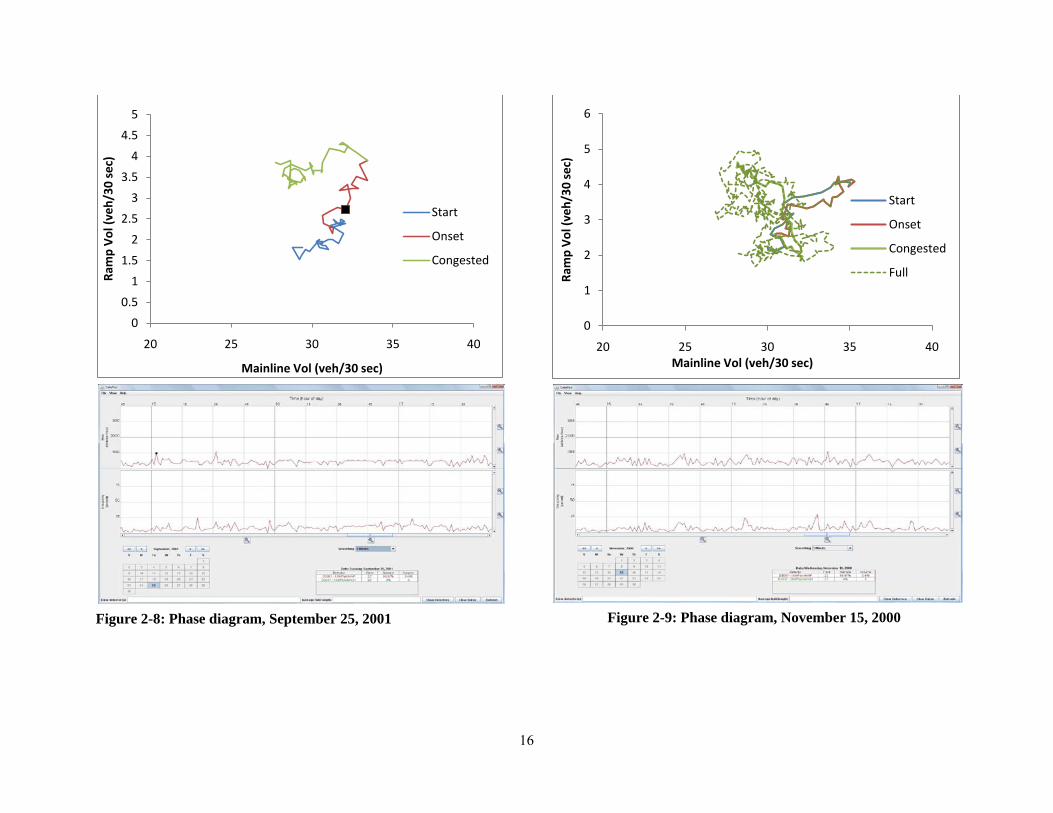
Phase Diagrams In order to better understand the capacity drop and to test how it changes with time (varying demand / varying control strategy implementations), we make use of a bottleneck flow contribution plot, a phase diagram. By plotting the flow volumes at the ramp associated with the bottleneck against the flow volumes observed at the upstream mainline detector one can better understand the breakdown behavior of the bottleneck, and how capacity changes during the duration of the breakdown (onset of congestion). In order to incorporate the time element into the graphs, we distinguish between the various phases: pre-congestion free flow regime, onset of congestion when speeds continue to decrease, and post breakdown congested regime, each represented by a different shade of the plot. Thus we can follow the behavior as the breakdown happens. Further, we support this plot with a time series plot of the demands on the ramp (using traffic states both at the merge detector and at the queue detector whenever available) which would help identify demand fluctuations on the ramp. Figure 2-6 through Figure 2-9 show the bottleneck flow contribution plots for various days in 2000 (simple Zone Metering), 2001 (No metering), and 2008 (Stratified Zone Metering). The first part of the figures shows the phase diagrams between on-ramp and mainline flow for different days. The second part of the figure shows the time series of metering rates (flow) at the downstream on-ramp detector and the occupancy measures at the upstream queue on-ramp detectors. For earlier years (2000, 2001) occupancy is for downstream ramp detectors, as queue detectors were not instrumented at that time. An isoquant in the phase diagrams, can be defined as the line connecting all flow contribution points on the plot that sum up to a certain total (ramp volume + mainline volume = constant). Since the scale along the ‘ramp volume’ axis is much smaller than the corresponding ‘mainline

13

volumes’ axis, the isoquants are along lines with a very steep negative slope. The horizontal separation between portions of the curve would thus represent the change in capacity. Certain spikes in the demands on the ramp are highlighted, both in the flow contribution plots as well as the demand time series graphs for better understanding.

14

2

2.5

3

3.5

4

4.5

5

25 27 29 31 33 35

Ram

p V

ol (v

eh/3

0 se

c)

Mainline vol (veh/30 sec)

Start

Onset

Congested

Figure 2-6: Phase diagram and demand at ramp, September 17, 2008

The mainline volume is plotted against the ramp volumes at the site of the bottleneck. Also shown is the time series plot of ramp volumes: Q detector demand volumes, and Merge detector supply volumes.

15

1

1.5

2

2.5

3

3.5

4

4.5

5

25 27 29 31 33 35

Ram

p V

ol (v

eh/3

0 se

c)

Mainline Vol (veh/30 sec)

Start

Onset

Congested

Figure 2-7: Phase diagram and demand at ramp, September 10, 2008

16

0

0.5

1

1.5

2

2.5

3

3.5

4

4.5

5

20 25 30 35 40

Ram

p V

ol (v

eh/3

0 se

c)

Mainline Vol (veh/30 sec)

Start

Onset

Congested

Figure 2-8: Phase diagram, September 25, 2001

0

1

2

3

4

5

6

20 25 30 35 40

Ram

p V

ol (v

eh/3

0 se

c)

Mainline Vol (veh/30 sec)

Start

Onset

Congested

Full

Figure 2-9: Phase diagram, November 15, 2000

17

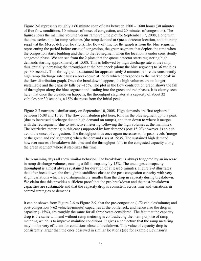
Figure 2-6 represents roughly a 60 minute span of data between 1500 – 1600 hours (30 minutes of free flow conditions, 10 minutes of onset of congestion, and 20 minutes of congestion). The figure shows the mainline volume versus ramp volume plot for September 17, 2008, along with the time series plot for ramp volumes (the ramp demand at Queue detector location, and the ramp supply at the Merge detector location). The flow of time for the graph is from the blue segment representing the period before onset of congestion, the green segment that depicts the time when the congestion starts building and then to the red segment when the location is under consistently congested phase. We can see from the 2 plots that the queue detector starts registering high demands starting approximately at 15:08. This is followed by high discharge rate at the ramp, thus, initially increasing the throughput at the bottleneck (along the blue segment) to 36 vehicles per 30 seconds. This throughput is sustained for approximately 5 minutes before the consistently high ramp discharge rate causes a breakdown at 15:15 which corresponds to the marked peak in the flow distribution graph. Once the breakdown happens, the high volumes are no longer sustainable and the capacity falls by ~15%. The plot in the flow contribution graph shows the fall of throughput along the blue segment and leading into the green and red phases. It is clearly seen here, that once the breakdown happens, the throughput stagnates at a capacity of about 32 vehicles per 30 seconds, a 15% decrease from the initial peak. Figure 2-7 narrates a similar story on September 10, 2008. High demands are first registered between 15:08 and 15:20. The flow contribution plot here, follows the blue segment up to a peak (due to increased discharge due to high demand on ramps), and then down to where it merges with the red segment (due to restrictive metering following the high volumes at the mainline). The restrictive metering in this case (supported by low demands post 15:20) however, is able to avoid the onset of congestion. The throughput thus once again increases to its peak levels (merge or the green and red segments) when the demand rises at 15:35. The sustained high demand however causes a breakdown this time and the throughput falls to the congested capacity along the green segment where it stabilizes this time. The remaining days all show similar behavior. The breakdown is always triggered by an increase in ramp discharge volumes, causing a fall in capacity by 15%. The uncongested capacity throughput is almost always sustained for duration of at least 5 minutes. Figure 2-9 illustrates that after breakdown, the throughput stabilizes close to the post-congestion capacity with very slight variations which are distinguishably smaller than the drop in capacity during breakdown. We claim that this provides sufficient proof that the pre-breakdown and the post-breakdown capacities are sustainable and that the capacity drop is consistent across time and variations in control strategies or demands. It can be shown from Figure 2-6 to Figure 2-9, that the pre-congestion (~72 vehicles/minute) and post-congestion (~62 vehicles/minute) capacities at the bottleneck, and hence also the drop in capacity (~15%), are roughly the same for all three years considered. The fact that the capacity drop is the same with and without ramp metering is contradicting the main purpose of ramp metering which is to improve mainline conditions. It gives a conjecture that the ramp metering may not be very efficient for conditions close to breakdown. This value of capacity drop is consistently larger than the ones observed in similar locations (see for example Levinson’s

18

study). The main reason for this very high value of drop is the extremely high values of ramp flows a few minutes before the occurrence of the breakdown. As seen in Figure 2-10, capacity before breakdown at 3:37pm is around 4400vh/hr. The high increase in ramp flows (~1000vh/hr) creates a breakdown and the flow after 5 minutes decreases to 3600vh/hr followed by a speed decrease (<35mph). Downstream of this location speed is still close to 60mph. Demand decreases and speed returns close to free-flow value around 4:05. At this time queue ramp constraint is violated and ramp rates increase again. A 2nd breakdown occurs and we observe approximately the same flow decrease (from 4400 to 3600vh/hr). Very high ramp rates continue to occur and the result is a further decrease in the bottleneck output (~2800vh/hr). The reason for this inefficiency is that the number of vehicles entered the freeway is very large and density increases at values which the bottleneck cannot discharge at capacity. We do not consider this as capacity drop because density is much higher than the critical value of density. Nevertheless, it is clear that despite the fact that there is no restriction downstream vehicles cannot discharge at higher values of flow as their speed is very small (~10mph). After 5:15pm the ramp rates decrease and the discharge flow of the bottleneck increases again to 3600vh/hr (bottleneck is still active until 5:55).

0

200

400

600

800

1000

1200

1400

0

1000

2000

3000

4000

3:32 3:42 3:52 4:02 4:12 4:22 4:32 4:42 4:52 5:02 5:12

Ram

p ra

te (v

h/hr

)

tota

l thr

ough

put (

vh/h

r)

Figure 2-10: Time series of throughput and ramp discharge rate at bottleneck

There is also an interesting observation that is derived directly from some of the flow contribution plots by observing the inclination of the curves to the two axes. The inclination (during the congested phase) from Figure 2-6 suggests that the volumes stabilize along an inclination that represents a ratio roughly equal to 2:1 between the mainline and ramp. This would imply that the isoquants are not equally distributed between the mainline and the ramp, and that an additional vehicle on the ramp is twice as detrimental to the congestion level at the bottleneck, as two additional vehicles on the mainline. However, this is not an easy attribute to be observed (since such an observation can only be made if the bottleneck remains close to full

19

capacity, and thus in the same isoquant, for an extended duration) more bottlenecks need to be explored and with a vaster time horizon in order to be able to support such a proposition. The various plots however, give consistent and convincing proof towards the existence of capacity drops. We currently analyze additional locations and the same patterns occur, which connect the magnitude of the capacity drop with the ramp rates.

20

21

Chapter 3 DENSITY PROFILE MODELING

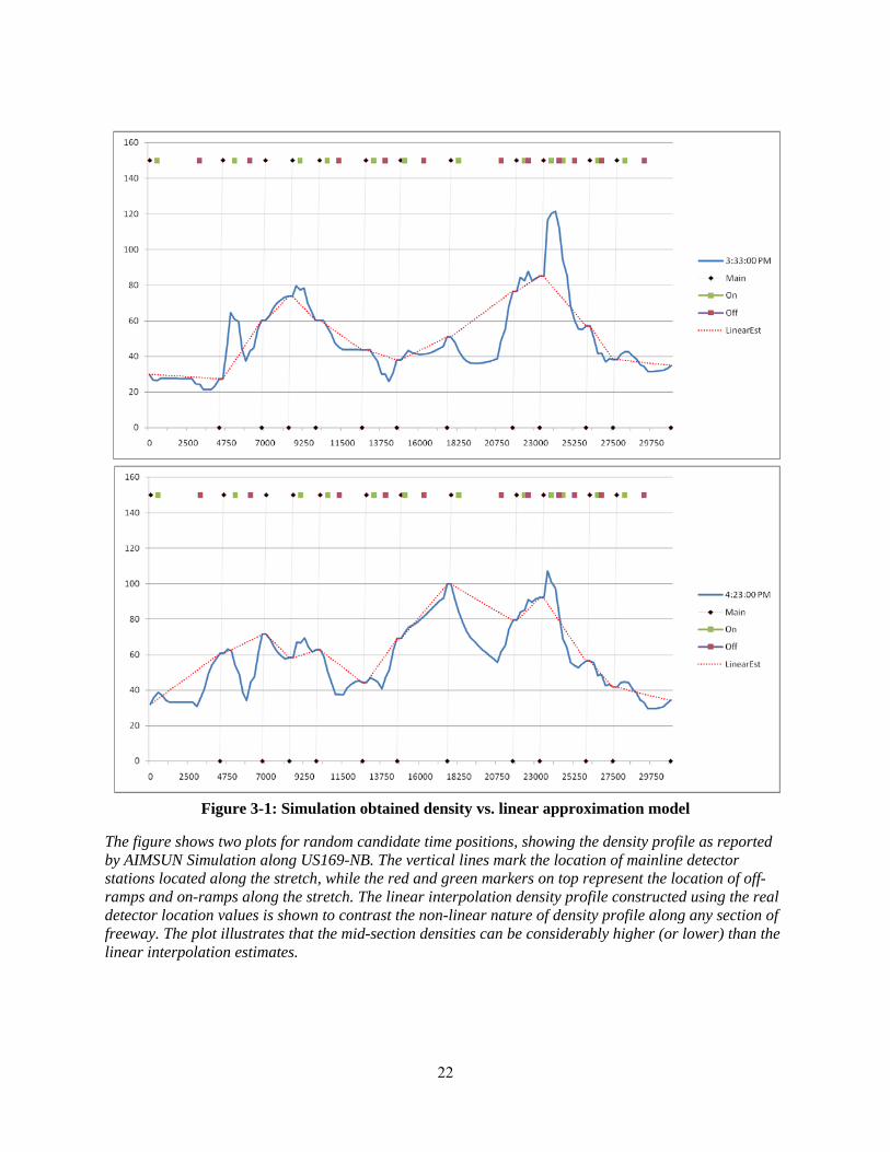
Density Modeling After describing the behavior of capacity drop, we next attempt to model the density distribution along a stretch of a highway section, using traffic data collected at the available detectors along the mainline and along the ramps. Current metering strategies based on density information use either a linear interpolation of density between known detector locations, or simple assuming the maximum / minimum at either ends of a section, for estimating the congestion level within the extent of a section. The actual bottlenecks are however usually likely to form closer to where the ramp merges into the freeway and thus often considerably away from the location of the detectors. The detectors are often not placed close to the actual merge intentionally since such locations witness a lot of lane changing movements and detectors are often not capable of accurately catching the right counts / densities under such situations. Thus, the densities that are observed at the two ends (upstream and downstream) of a section of freeway are often lower than the peak density witnessed along the section. Using simulation data obtained for densities along a freeway section, we first show that linear interpolation approximations, from known detector locations, can have high errors (both positive and negative). Once a need for a better profiling of density along the section has been established, we propose a simple model that can be efficiently used to predict densities along the stretch and then follow it with some comparison studies done against simulation data. For the purpose of the study, we use the stretch of US Highway 169 Northbound, between its intersection with Valley View Road (at the upstream end) and with County Road 10 (at the downstream end). We specifically look at the congestion section along the highway between its intersection with Excelsior Boulevard at the upstream end and with Plymouth Avenue at the downstream end for some of the analysis. The Plymouth Avenue on ramp to US 169 was a site of an active bottleneck consistently. We model the traffic behavior along the highway stretch using AIMSUN (microscopic traffic simulation software). The simulator uses demand values at all access points to the network, as well as using turning movement percentages at any decision point (such as an off ramp) as input. Data obtained from real measurements from detectors along the freeway stretch provide both the demands at entries along the network, as well as the turning percentages at decision points. Additional detectors were placed along the stretch of freeway being studied in order to catch the traffic states between actual detector locations. Traffic state data collected for all the detectors along the freeway network, as reported by the simulator can be used to create a density profile along the stretch. This density profile obtained through the simulation is compared against a simple linear interpolation from real available mainline detector readings, as shown in Figure 3-1. Figure 3-1 shows density values (in vehicles/mile) vs. distance (in feet) for two different time instances. The figure shows that the actual density profile observed within a section is not linear in nature and thus can’t be estimated accurately with a linear interpolation scheme. Linear interpolation estimation can easily underestimate or overestimate the density at an intermediate location within a section as evident from the figure. The error levels in the linear estimation model is clearly visible, thus demanding a better estimation model in order to more effectively predict realistic congestion levels within a section.

22

Figure 3-1: Simulation obtained density vs. linear approximation model

The figure shows two plots for random candidate time positions, showing the density profile as reported by AIMSUN Simulation along US169-NB. The vertical lines mark the location of mainline detector stations located along the stretch, while the red and green markers on top represent the location of off-ramps and on-ramps along the stretch. The linear interpolation density profile constructed using the real detector location values is shown to contrast the non-linear nature of density profile along any section of freeway. The plot illustrates that the mid-section densities can be considerably higher (or lower) than the linear interpolation estimates.

23

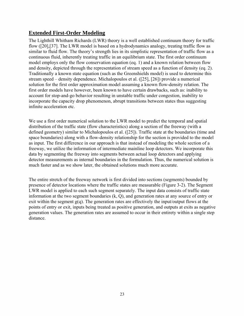
Extended First-Order Modeling The Lighthill Whitham Richards (LWR) theory is a well established continuum theory for traffic flow ([20],[37]. The LWR model is based on a hydrodynamics analogy, treating traffic flow as similar to fluid flow. The theory’s strength lies in its simplistic representation of traffic flow as a continuous fluid, inherently treating traffic in an equilibrium state. The first order continuum model employs only the flow conservation equation (eq. 1) and a known relation between flow and density, depicted through the representation of stream speed as a function of density (eq. 2). Traditionally a known state equation (such as the Greenshields model) is used to determine this stream speed – density dependence. Michalopoulos et al. ([25], [26]) provide a numerical solution for the first order approximation model assuming a known flow-density relation. The first order models have however, been known to have certain drawbacks, such as: inability to account for stop-and-go behavior resulting in unstable traffic under congestion, inability to incorporate the capacity drop phenomenon, abrupt transitions between states thus suggesting infinite acceleration etc. We use a first order numerical solution to the LWR model to predict the temporal and spatial distribution of the traffic state (flow characteristics) along a section of the freeway (with a defined geometry) similar to Michalopoulos et al. ([25]). Traffic state at the boundaries (time and space boundaries) along with a flow-density relationship for the section is provided to the model as input. The first difference in our approach is that instead of modeling the whole section of a freeway, we utilize the information of intermediate mainline loop detectors. We incorporate this data by segmenting the freeway into segments between actual loop detectors and applying detector measurements as internal boundaries in the formulation. Thus, the numerical solution is much faster and as we show later, the obtained solutions much more accurate. The entire stretch of the freeway network is first divided into sections (segments) bounded by presence of detector locations where the traffic states are measurable (Figure 3-2). The Segment LWR model is applied to each such segment separately. The input data consists of traffic state information at the two segment boundaries (k, Q), and generation rates at any source of entry or exit within the segment g(q). The generation rates are effectively the input/output flows at the points of entry or exit, inputs being treated as positive generation, and outputs at exits as negative generation values. The generation rates are assumed to occur in their entirety within a single step distance.

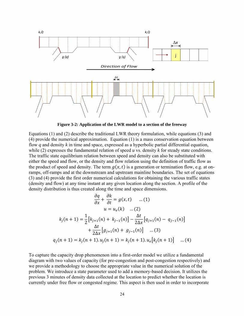
24

Figure 3-2: Application of the LWR model to a section of the freeway

Equations (1) and (2) describe the traditional LWR theory formulation, while equations (3) and (4) provide the numerical approximation. Equation (1) is a mass conservation equation between flow q and density k in time and space, expressed as a hyperbolic partial differential equation, while (2) expresses the fundamental relation of speed u vs. density k for steady state conditions. The traffic state equilibrium relation between speed and density can also be substituted with either the speed and flow, or the density and flow relation using the definition of traffic flow as the product of speed and density. The term 𝑔(𝑥, 𝑡) is a generation or termination flow, e.g. at on-ramps, off-ramps and at the downstream and upstream mainline boundaries. The set of equations (3) and (4) provide the first order numerical calculations for obtaining the various traffic states (density and flow) at any time instant at any given location along the section. A profile of the density distribution is thus created along the time and space dimensions.

𝜕𝑞𝜕𝑥

𝑢 = 𝑢𝑒(𝑘) … (2)

𝑘𝑗(𝑛 + 1) =12�𝑘𝑗+1(𝑛) + 𝑘𝑗−1(𝑛)� −

∆𝑡2∆𝑥

�𝑞𝑗+1(𝑛) − 𝑞𝑗−1(𝑛)�

+∆𝑡

2∆𝑥�𝑔𝑗+1(𝑛) + 𝑔𝑗−1(𝑛)� … (3)

+ 𝜕𝑘𝜕𝑡

= 𝑔(𝑥, 𝑡) … (1)

𝑞𝑗(𝑛 + 1) = 𝑘𝑗(𝑛 + 1).𝑢𝑗(𝑛 + 1) = 𝑘𝑗(𝑛 + 1).𝑢𝑒�𝑘𝑗(𝑛 + 1)� … (4) To capture the capacity drop phenomenon into a first-order model we utilize a fundamental diagram with two values of capacity (for pre-congestion and post-congestion respectively) and we provide a methodology to choose the appropriate value in the numerical solution of the problem. We introduce a state parameter used to add a memory-based decision. It utilizes the previous 3 minutes of density data collected at the location to predict whether the location is currently under free flow or congested regime. This aspect is then used in order to incorporate

25

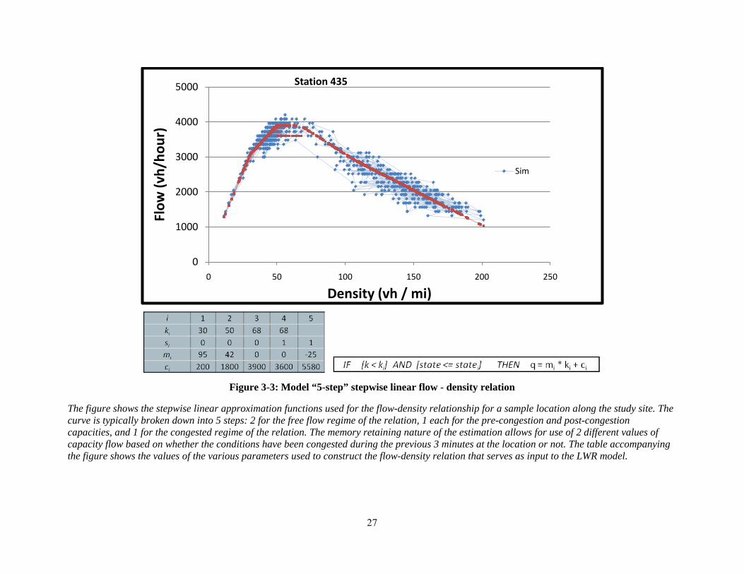
the effect of capacity drop. Thus, for the same density value, a higher flow is estimated (corresponding to free flow capacity) if the average density observed over the previous 3 minutes was lower than the critical density for the location, while a lower flow is estimated (corresponding to congested capacity) if the location has been in congestion. The given section is divided into sub-parts each of a length Δx which form the location/distance steps, and the time horizon is similarly divided into time steps each Δt seconds of length. Ideally the relation Δx/Δt should be close to the free flow speed on the section being studied. The inputs to the model then consist of: (1) the flow and the density information at the boundaries of the freeway section (at the upstream boundary and the downstream boundary) at all time steps, (2) the flow and density at each location at time zero along the length of the section, (3) flow at all sources (on-ramps), and sinks (off-ramps) along the section, and (4) the flow-density relation for traffic in the given section. Figure 3-2 shows a representation of how the model is constructed. Previous studies have been able to utilize such a first order estimation model to predict the density / flow profile along a section of freeway. These studies have used the entire freeway stretch as a single unit and applied the model on the entire stretch thus using the traffic state data only at the upstream and the downstream extremes as input. A segmented LWR model, that treats each section (stretch of freeway between two consecutive available detector stations) as a separate unit, thus computing the distribution of density separately for each section, can more effectively utilize all the available detector information. Such a method is not only bound to have a higher accuracy (since errors can no longer propagate along space), but is also computationally more efficient (since each model is applied for a single section, and hence the computational load can potentially be distributed). Furthermore, the LWR model needs an intrinsic relationship definition between the flow and the density at all locations along the stretch being modeled. We propose here, that using a simple stepwise linear estimation of the flow-density relation, while accounting for the capacity drop phenomenon, can greatly help increase the accuracy of the modeling while keeping the computational effort light. Figure 3-3 and Figure 3-4 show the MFD (flow density relationship) estimation used for this purpose for two sample locations along the freeway. The fundamental flow – density relation for any section, is approximated through a 5-step piecewise linear model. Each step is represented by a conditional block when defining the flow-density relation in the LWR model. The model thus computes the correct flow value corresponding to a given density, by sequentially going through all the conditional blocks that are used to define the relation. Each block i is defined by a set of 4 values: density boundary between block i and i+1, 𝑘𝑖; congestion state, 𝑠𝑖 (with value 0 for uncongested and 1 for congested); flow axis intercept, 𝑐𝑖 and slope, 𝑚𝑖 (together define the shape of the linear relation pertaining to the current step). The congestion state, 𝑠𝑖 is used to provide the memory-based decision system while deciding the capacity flow to be used whenever required. The first two blocks typically represent the uncongested phase of traffic. Block 1 is for light conditions where vehicles run at free-flow speed. Block 2 is also under-saturated, but the effect of vehicle interactions slightly decreases speed below free-flow. The next two blocks represent the pre-congestion and post-congestion capacities, while block 5 represents the behavior in the

26

congested phase at the location. The proposed Segmented LWR model thus incorporates both the segmented nature, and the memory based flow-density approximation model described to account for the capacity drop phenomenon as observed earlier.

27

0

1000

2000

3000

4000

5000

0 50 100 150 200 250

Flow

(vh/

hour

)

Density (vh / mi)

Station 435

Sim

Figure 3-3: Model “5-step” stepwise linear flow - density relation

The figure shows the stepwise linear approximation functions used for the flow-density relationship for a sample location along the study site. The curve is typically broken down into 5 steps: 2 for the free flow regime of the relation, 1 each for the pre-congestion and post-congestion capacities, and 1 for the congested regime of the relation. The memory retaining nature of the estimation allows for use of 2 different values of capacity flow based on whether the conditions have been congested during the previous 3 minutes at the location or not. The table accompanying the figure shows the values of the various parameters used to construct the flow-density relation that serves as input to the LWR model.

28

0

1000

2000

3000

4000

5000

0 50 100 150 200 250

Flow

(vh/

hour

)

Density (vh / mi)

Station 438

Sim

Model

Figure 3-4: Another example of the “5-step” estimations

Simulation Results The site used for study was a stretch of US Highway 169 Northbound, between its intersection with Valley View Road (at the upstream end) and with County Road 10 (at the downstream end). Thirty second traffic demand data was used as input for the simulation as the demand distribution and the turning percentages. The traffic state data was extracted directly from the Minnesota DOT loop detector database. This raw data was filtered for missing data and non operational detectors. For the purpose of the density profile study, only one peak period was tested, specifically the p.m. peak on September 25, 2008 between 2pm and 8pm. The densities obtained from the simulation and from the LWR models were also converted to 10 minute moving average values for comparison purposes wherever needed. Comparison is made between the simulation density results (treated as representing the real data), the full span LWR model, and the segmented LWR model through contour density plots, time series plots of density and density profiles along portions of the stretch at specific time instances. Figure 3-9 shows a contour plot depicting density (depth axis) profile against time (horizontal axis) and space (vertical axis) for the three cases being compared: AIMSUN simulation data, the Segmented LWR Model as proposed in the paper, and the simple Full Span LWR Model estimation results. The Segmented LWR model shows considerable improvement

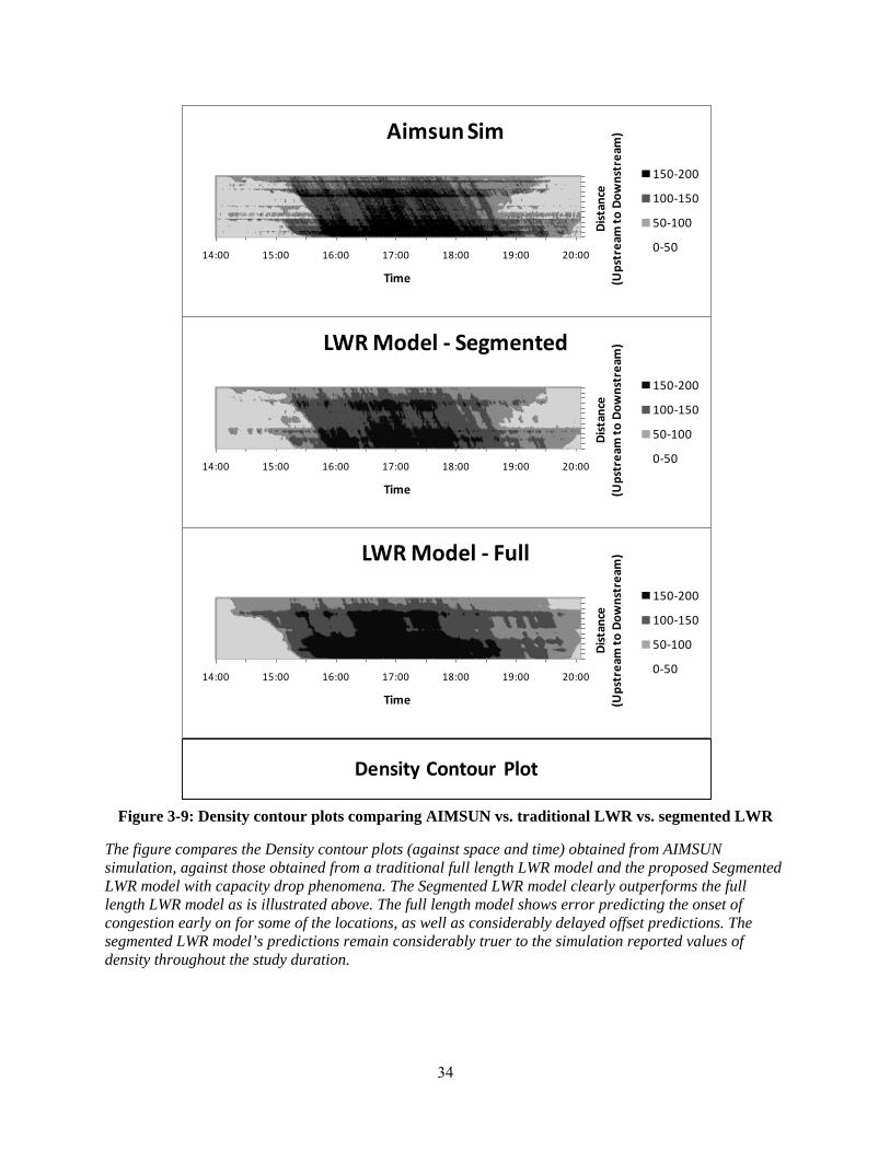
29

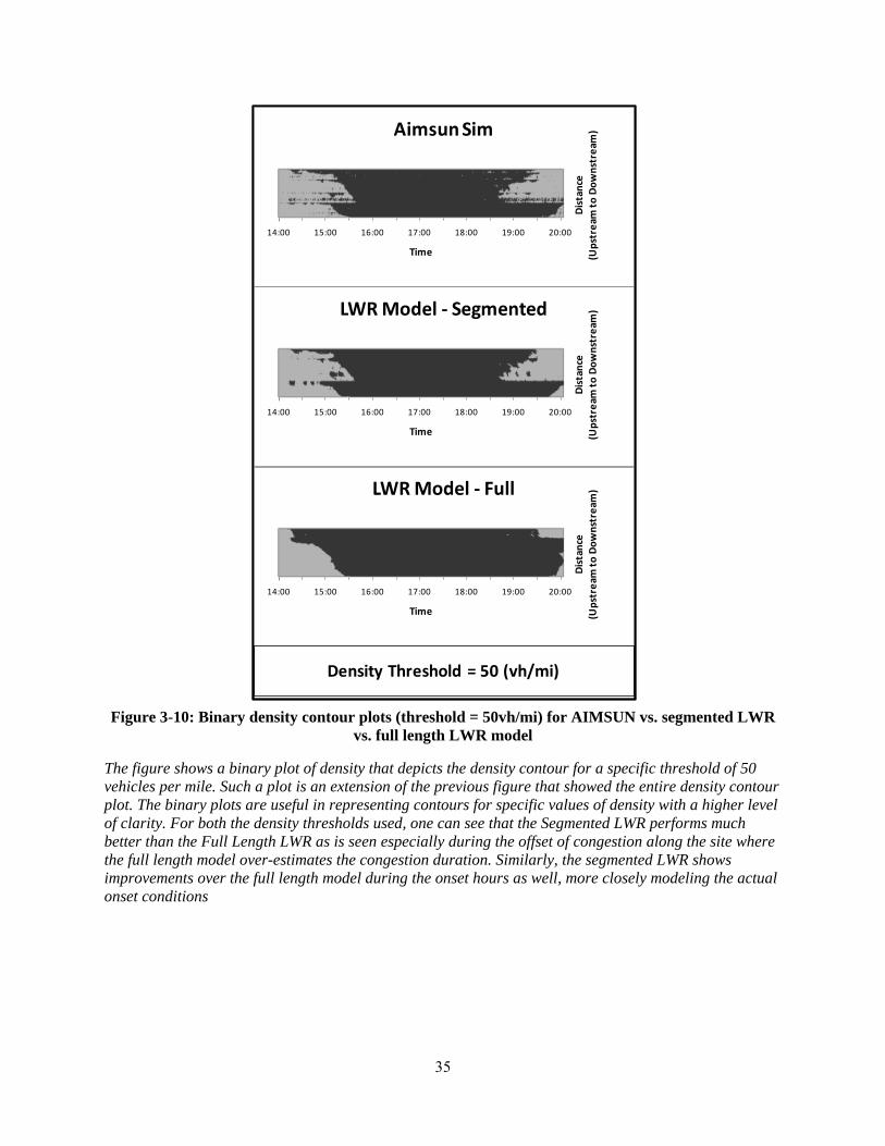
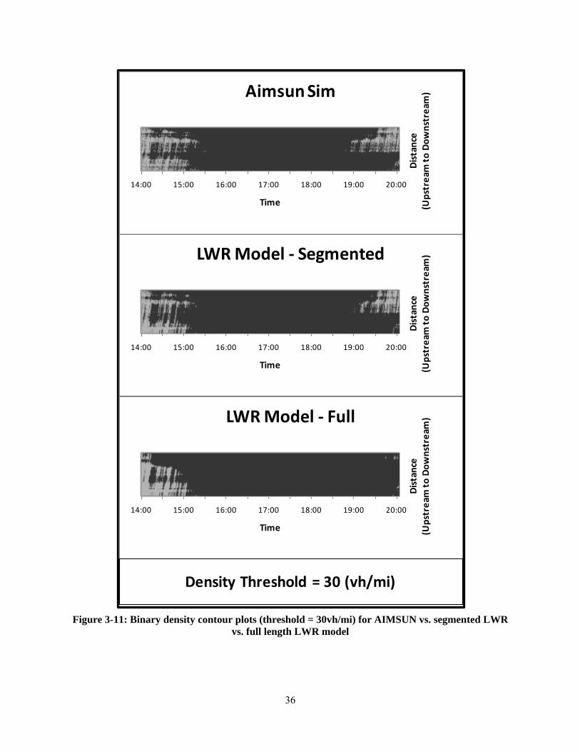
over the Full Span LWR Model in estimating the density profile as verified against the simulation generated profile. In order to further substantiate the estimation model’s strength, Binary Contour Plots are created for the three scenarios using different threshold density values. The Binary Contour Plot depicts the contour using a specific value of density (50 vehicles / mile) which closely approximates the critical density along the stretch, and 30 vehicles / mile as shown in Figure 3-10 and Figure 3-11. Thus, the plot depicts densities lower and higher than the threshold value in different colors respectively, also in the process, forming the contour boundary corresponding to the threshold density. Such a plot gives a clearer picture of how well a model can estimate the congestion boundaries (onset and offset) both in space and in time. The binary contour plots once again highlight the improvement of the segmented model, over the full span LWR model. The segmented model is in fact seen to predict the density profile to a high degree of accuracy, albeit with smoother transitions and less fluctuations when compared to the simulation based profile. While the full span model performs reasonably well pre-congestion (possibly associated with a relatively smooth relation between flow and density pre-congestion), as seen from the contour plots, the performance of the segmented model is considerably better for the congested and the post congestion regions (where flow has a higher range of scatter and is more stochastic for a given density). This suggests that the segmented model provides and improvement towards the accepted limitations of conventional full span model (high lane merging disruptions, stop and go traffic etc).

30

Figure 3-5: Density profile showing AIMSUN reported density vs. LWR predicted density against distance during an off-peak instance of

time

31

Figure 3-6: Density profile showing AIMSUN reported density vs. LWR predicted density against distance during a peak time instance

32

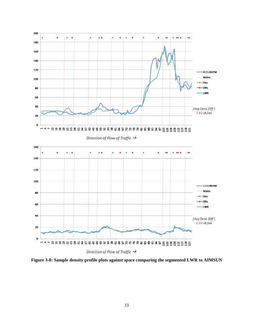
Figure 3-7: Sample density profile plots against space comparing the segmented LWR to AIMSUN

33

Figure 3-8: Sample density profile plots against space comparing the segmented LWR to AIMSUN

34

14:00 15:00 16:00 17:00 18:00 19:00 20:00

Dis

tanc

e (U

pstr

eam

to D

owns

trea

m)

Time

Aimsun Sim

150-200

100-150

50-100

0-50

14:00 15:00 16:00 17:00 18:00 19:00 20:00

Dis

tanc

e (U

pstr

eam

to D

owns

trea

m)

Time

LWR Model - Segmented

150-200

100-150

50-100

0-50

14:00 15:00 16:00 17:00 18:00 19:00 20:00

Dis

tanc

e (U

pstr

eam

to D

owns

trea

m)

Time

LWR Model - Full

150-200

100-150

50-100

0-50

Density Contour Plot

Figure 3-9: Density contour plots comparing AIMSUN vs. traditional LWR vs. segmented LWR

The figure compares the Density contour plots (against space and time) obtained from AIMSUN simulation, against those obtained from a traditional full length LWR model and the proposed Segmented LWR model with capacity drop phenomena. The Segmented LWR model clearly outperforms the full length LWR model as is illustrated above. The full length model shows error predicting the onset of congestion early on for some of the locations, as well as considerably delayed offset predictions. The segmented LWR model’s predictions remain considerably truer to the simulation reported values of density throughout the study duration.

35

14:00 15:00 16:00 17:00 18:00 19:00 20:00

Dis

tanc

e (U

pstr

eam

to D

owns

trea

m)

Time

Aimsun Sim

14:00 15:00 16:00 17:00 18:00 19:00 20:00D

ista

nce

(Ups

trea

m to

Dow

nstr

eam

)

Time

LWR Model - Full

14:00 15:00 16:00 17:00 18:00 19:00 20:00

Dis

tanc

e (U

pstr

eam

to D

owns

trea

m)

Time

LWR Model - Segmented

Density Threshold = 50 (vh/mi)

Figure 3-10: Binary density contour plots (threshold = 50vh/mi) for AIMSUN vs. segmented LWR vs. full length LWR model

The figure shows a binary plot of density that depicts the density contour for a specific threshold of 50 vehicles per mile. Such a plot is an extension of the previous figure that showed the entire density contour plot. The binary plots are useful in representing contours for specific values of density with a higher level of clarity. For both the density thresholds used, one can see that the Segmented LWR performs much better than the Full Length LWR as is seen especially during the offset of congestion along the site where the full length model over-estimates the congestion duration. Similarly, the segmented LWR shows improvements over the full length model during the onset hours as well, more closely modeling the actual onset conditions

36

14:00 15:00 16:00 17:00 18:00 19:00 20:00

Dis

tanc

e (U

pstr

eam

to D

owns

trea

m)

Time

Aimsun Sim

14:00 15:00 16:00 17:00 18:00 19:00 20:00

Dis

tanc

e (U

pstr

eam

to D

owns

trea

m)

Time

LWR Model - Full

14:00 15:00 16:00 17:00 18:00 19:00 20:00

Dis

tanc

e (U

pstr

eam

to D

owns

trea

m)

Time

LWR Model - Segmented

Density Threshold = 30 (vh/mi)

Figure 3-11: Binary density contour plots (threshold = 30vh/mi) for AIMSUN vs. segmented LWR vs. full length LWR model

37

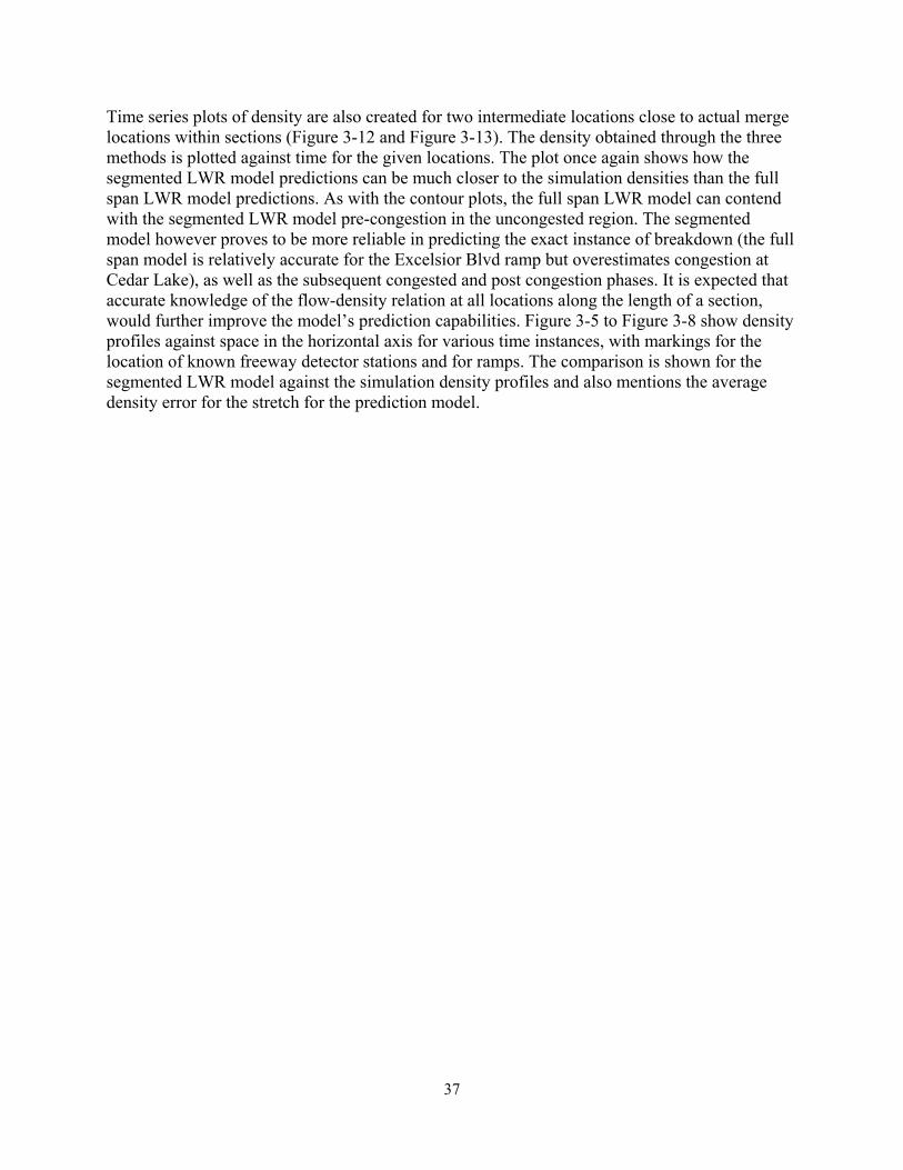
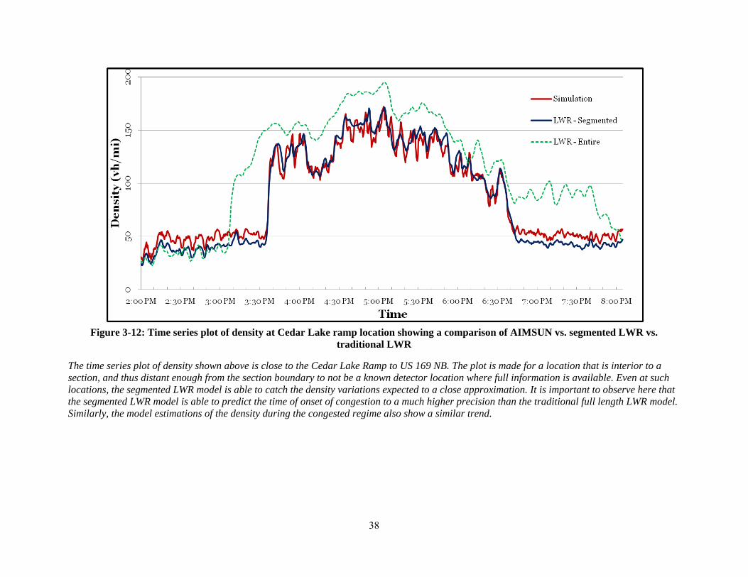
Time series plots of density are also created for two intermediate locations close to actual merge locations within sections (Figure 3-12 and Figure 3-13). The density obtained through the three methods is plotted against time for the given locations. The plot once again shows how the segmented LWR model predictions can be much closer to the simulation densities than the full span LWR model predictions. As with the contour plots, the full span LWR model can contend with the segmented LWR model pre-congestion in the uncongested region. The segmented model however proves to be more reliable in predicting the exact instance of breakdown (the full span model is relatively accurate for the Excelsior Blvd ramp but overestimates congestion at Cedar Lake), as well as the subsequent congested and post congestion phases. It is expected that accurate knowledge of the flow-density relation at all locations along the length of a section, would further improve the model’s prediction capabilities. Figure 3-5 to Figure 3-8 show density profiles against space in the horizontal axis for various time instances, with markings for the location of known freeway detector stations and for ramps. The comparison is shown for the segmented LWR model against the simulation density profiles and also mentions the average density error for the stretch for the prediction model.

38

Figure 3-12: Time series plot of density at Cedar Lake ramp location showing a comparison of AIMSUN vs. segmented LWR vs.

traditional LWR

The time series plot of density shown above is close to the Cedar Lake Ramp to US 169 NB. The plot is made for a location that is interior to a section, and thus distant enough from the section boundary to not be a known detector location where full information is available. Even at such locations, the segmented LWR model is able to catch the density variations expected to a close approximation. It is important to observe here that the segmented LWR model is able to predict the time of onset of congestion to a much higher precision than the traditional full length LWR model. Similarly, the model estimations of the density during the congested regime also show a similar trend.

39

Figure 3-13: Time series plot of density at Excelsior Blvd. ramp to US 169 NB comparing AIMSUN to Segmented LWR and traditional

LWR model estimations

The full span model shows better results at this location as compared to the previous location post congestion. Excelsior Blvd being closer to the upstream boundary of congestion and thus nearer to the uncongested boundary might be an explanation for this behavior. However, the performance of the full span model post congestion shows a lot of fluctuations from one site to another.

40

Conclusions The study of the freeway data from the Twin Cities Metropolitan Area provides clear evidence of a capacity drop phenomenon. This is further supported by the use of phase diagram to observe and quantify the capacity drop and to also observe the triggers to the collapse of capacity. Further, it is shown that this capacity drop is not affected greatly by the kind of metering strategy in place. This is shown through a comparison of the drops observed over various years: (i) in 2000 when ramp metering strategy did not have any ramp delay constraints, (ii) in 2001 when ramp metering was out of operation and access to freeways was not controlled, and (iii) in 2008 when the Stratified Zone Metering strategy was in place with ramp delay constraints in place. In all cases capacity drop phenomenon were of the same magnitude not affected by the different type of ramp control strategy. In the second part of the chapter a methodology was developed to estimate densities profiles in space in time dimensions based on data from loop detectors. The methodology is based on solving a flow conservation differential equation (using LWR theory) with intermediate or internal freeway mainline boundaries, which makes the calculation faster and more accurate compared to traditional LWR based estimations that use only external boundaries of the system. In order to capture the capacity drop phenomenon into the first-order model, a stepwise linear fundamental diagram / flow-density relation can be employed. This stepwise linear interpretation of the fundamental diagram employs the use of dual capacity values and a memory-based methodology is used to choose the appropriate capacity value in the numerical solution of the problem. Results compared with micro-simulation of highway US169-NB stretch show that this model produces more reliable results than previous theories.

41

Chapter 4 RAMP METERING AND OBSERVATIONS

On-ramp metering has been widely employed as an effective strategy to reduce congestion and increase freeway operational efficiency. It is one of the most efficient tools to mitigate congestion, other than adding more capacity to transportation infrastructures. The fundamental philosophy of ramp metering is that a corridor can maintain its optimal operation by regulating the freeway demand to be under its capacity. Over the years, a number of traffic-responsive ramp control strategies have been developed in order to regulate the entrance ramp demand to freeways. These strategies use basic principles of feedback and feed-forward controls with minor modifications and can be classified as isolated or coordinated. In isolated ramp-metering algorithms, the rate for an on-ramp is determined based on its local traffic conditions. The most prominent example of isolated metering strategy with multiple successful field applications (Amsterdam, Paris, Glasgow, Munich etc) is ALINEA, which targets a set point for the downstream occupancy or density [33]. A review of other isolated algorithms is presented in Papageorgiou and Kotsialos [31]. The main inefficiencies of isolated ramp algorithms are in case of (i) high demand, where inequity issues arise, as travelers at the on-ramps experience significantly higher delays than those in the mainline or adjacent ramps (ii) short on-ramps, where long queues can spillback in the arterial network and create significant delays in urban streets and (iii) multiple active bottlenecks. Coordinated ramp-metering strategies utilize system-wide traffic measurements from an entire region of the network to control all on-ramps within the region. Some operational examples of coordinated algorithms are the Bottleneck [16], Zone [38], Metaline [32], Helper [21] and Swarm [28]. A variety of optimal control theories coupled with dynamic traffic simulation models have been applied in [39],[43],[17],[11],[34]. The objective for most of these studies is to minimize the total system travel time including ramp delay. An extensive review of heuristic coordinated traffic-responsive ramp-metering algorithms is presented in [2], [45]. A more advanced concept in freeway control (similar to the coordinated one) employs a hierarchical control structure, where overall freeway control is decomposed into several components or layers, such as prediction, optimization and direct control. The main objective of hierarchical control is to achieve computational feasibility and robustness of the control solutions by determining the system-wide, nominal metering rates first and then adjusting them according to real traffic conditions. Previous efforts have employed the hierarchical control concept based on two, three or four layers. Papageorgiou [29] proposed a three layer control system consisting of an optimization, a direct control and an adaptation layer. Four layer hierarchical control, as proposed by May [24], includes initialization, estimation, optimization and tactics processors. The Stratified Ramp Control (SZM), deployed by Mn/DOT [19], is essentially three-layer, including ramp, zone and system layer (i.e., broken zone identification layer) design. Total ramp volume is distributed over all metered ramps in the zone in proportion to their demands. The Stratified Ramp Control targets the flow capacity in the merge area and is based on mainstream and ramp measurements of flow and occupancy. Further extensions to this algorithm include

42

improvements for the determination of the ramp minimum release rate [10] and the queue size estimation [22]. All the aforementioned strategies for Minnesota’s freeways are relying on capacity estimations from traffic flows. However, analysis of real traffic data from freeway merge areas indicates that the recurrent traffic breakdown during peak hours can occur at different flow values, even under the same weather and lighting conditions ([9], 74[23]). Furthermore, probabilistic characteristics of capacity have been observed broadly in the literature, e.g. [18], due to breakdown phenomena or variability of weather conditions. On the other hand, earlier research [6] indicates that the critical value of occupancy at which capacity is observed, is less sensitive and quite stable. Our own research on the subject in Minnesota’s freeways confirms the above findings and indicates a capacity drop of as high as 20% resulting in substantial miscalculation of the optimal metering rates. This suggests that a control strategy based on flow thresholds is likely to under-load the freeway or lead to traffic congestion. Therefore, it is desirable to develop a new methodology to overcome this randomness to make the Stratified Ramp Control strategy more robust and more adaptive to the freeway geometry and real time traffic conditions. The algorithm presented is prepared following a number of discussions with Mn/DOT which first identified the need to move to the new generation based on density considerations rather than flows. In addition, the principles of the current scheme were developed in the late 60's; albeit the recent ramp queue improvements were only deployed in 2003, the main line modeling has not changed. Thus, the new generation should have a major impact in both the state of the practice and the state of the art. A field test implementation of the resulting control strategy, currently being planned, is essential for refinements and large scale deployment in the Twin Cities freeway. In this chapter we present some empirical observations for the current algorithm from the Twin Cities Metropolitan area. This is followed by a description of the new density-based, coordinated algorithm and an implementation to a 12-mile corridor at the H-169 freeway through micro-simulation.

Ramp Metering in Minnesota Minnesota has had a long history of ramp metering algorithms. Minnesota’s original ZONE algorithm employed the definition of zones within which on-ramp access was controlled based on simple conservation of mass relations. The ZONE algorithm thus gave priority to the mainline freeway traffic and working towards avoiding congestion on the freeway by controlling the metering rates on the ramps. In late 2000, following some raised concerns about how effective Minnesota’s ramp metering really was, the Minnesota legislature mandated a study to be performed by turning off all existing ramp meters for a 6 week period starting Oct 2000. The objective of the study was to perform a ‘before’ and ‘after’ study of traffic conditions comparing the effects of presence and absence of freeway metering. The results seen from the study showed that metering not only improved the performance level of the freeways by reducing delays and total travel times, but also reduced incident rates along the freeway system.

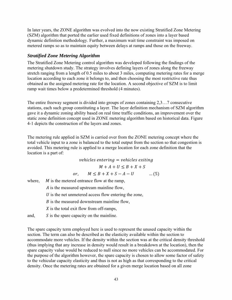
43

In later years, the ZONE algorithm was evolved into the now existing Stratified Zone Metering (SZM) algorithm that ported the earlier used fixed definitions of zones into a layer based dynamic definition methodology. Further, a maximum wait time constraint was imposed on metered ramps so as to maintain equity between delays at ramps and those on the freeway.

Stratified Zone Metering Algorithm The Stratified Zone Metering control algorithm was developed following the findings of the metering shutdown study. The strategy involves defining layers of zones along the freeway stretch ranging from a length of 0.5 miles to about 3 miles, computing metering rates for a merge location according to each zone it belongs to, and then choosing the most restrictive rate thus obtained as the assigned metering rate for the location. A second objective of SZM is to limit ramp wait times below a predetermined threshold (4 minutes). The entire freeway segment is divided into groups of zones containing 2,3…7 consecutive stations, each such group constituting a layer. The layer definition mechanism of SZM algorithm gave it a dynamic zoning ability based on real time traffic conditions, an improvement over the static zone definition concept used in ZONE metering algorithm based on historical data. Figure 4-1 depicts the construction of the layers and zones. The metering rule applied in SZM is carried over from the ZONE metering concept where the total vehicle input to a zone is balanced to the total output from the section so that congestion is avoided. This metering rule is applied to a merge location for each zone definition that the location is a part of:

𝑣𝑒ℎ𝑖𝑐𝑙𝑒𝑠 𝑒𝑛𝑡𝑒𝑟𝑖𝑛𝑔 = 𝑣𝑒ℎ𝑖𝑐𝑙𝑒𝑠 𝑒𝑥𝑖𝑡𝑖𝑛𝑔

𝑀 + 𝐴 + 𝑈 ≤ 𝐵 + 𝑋 + 𝑆𝑜𝑟, 𝑀 ≤ 𝐵 + 𝑋 + 𝑆 − 𝐴 − 𝑈 … (5)

where,

𝑈

is the metered entrance flow at the ramp,

𝐵

is the measured upstream mainline flow,

𝑋

is the net unmetered access flow entering the zone,

𝑆

is the measured downstream mainline flow, is the total exit flow from off-ramps, and, is the spare capacity on the mainline. The spare capacity term employed here is used to represent the unused capacity within the section. The term can also be described as the elasticity available within the section to accommodate more vehicles. If the density within the section was at the critical density threshold (thus implying that any increase in density would result in a breakdown at the location), then the spare capacity value would be reduced to null since no more vehicles can be accommodated. For the purpose of the algorithm however, the spare capacity is chosen to allow some factor of safety to the vehicular capacity elasticity and thus is not as high as that corresponding to the critical density. Once the metering rates are obtained for a given merge location based on all zone

𝑀𝐴

44

assignments it forms a part of, the most restrictive flow rate measure is chosen and imposed on the ramp. Figure 4-2 summarizes the structure of the SZM algorithm. While the above introduction is aimed at giving an overview of the ideologies of the SZM strategy, one can refer to [27] for a concise description of all concepts involved in SZM, and [19], [41] for the full detail description of the SZM control strategy.

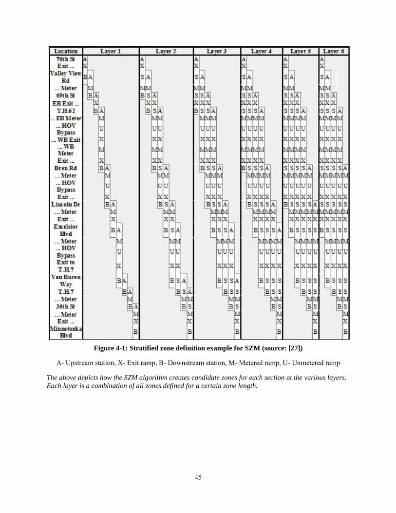
45

Figure 4-1: Stratified zone definition example for SZM (source: [27])

A- Upstream station, X- Exit ramp, B- Downstream station, M- Metered ramp, U- Unmetered ramp

The above depicts how the SZM algorithm creates candidate zones for each section at the various layers. Each layer is a combination of all zones defined for a certain zone length.

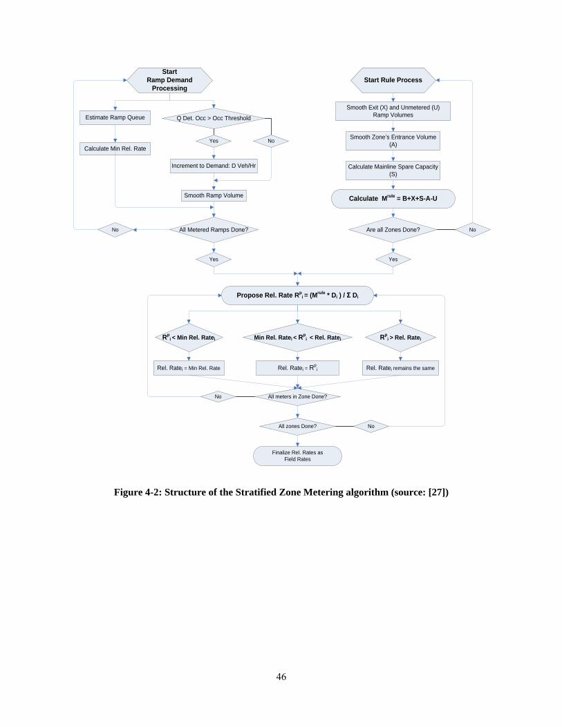
46

Estimate Ramp Queue

Start Ramp Demand

Processing

Q Det. Occ > Occ Threshold

Smooth Ramp Volume

No

All Metered Ramps Done?

Calculate Min Rel. Rate

No

Yes

Start Rule Process

Yes

Smooth Exit (X) and Unmetered (U) Ramp Volumes

Smooth Zone’s Entrance Volume (A)

Calculate Mainline Spare Capacity (S)

Calculate Mrule = B+X+S-A-U

Yes

Are all Zones Done?

Propose Rel. Rate Rpi = (Mrule * Di ) / Σ Di

Min Rel. Ratei < Rpi < Rel. RateiRp

i < Min Rel. Ratei Rpi > Rel. Ratei

Rel. Ratei = Rpi Rel. Ratei remains the sameRel. Ratei = Min Rel. Rate

All meters in Zone Done?

All zones Done?

No

No

No

Finalize Rel. Rates as Field Rates

Increment to Demand: D Veh/Hr

Figure 4-2: Structure of the Stratified Zone Metering algorithm (source: [27])

47

Observations about SZM Careful analysis of the current Stratified Zone Metering algorithm and the corresponding empirical data (detector readings and meter rates) of active bottlenecks in the Twin Cities Metropolitan Area revealed some interesting observations. The following were seen to occur on a frequent basis:

(i) Underutilized Capacity. The capacity before the occurrence of a breakdown at a bottleneck is often higher than the post-breakdown capacity as shown earlier. Using a fixed capacity value means that the capacity drop is not accounted for and a restrictive estimate of capacity value is used in the algorithm that underestimates the pre-breakdown capacity at the link. This also leads us to the next observation:

(ii) Over-estimated Capacity Post Breakdown. Once the freeway has reached a state of congestion, the actual capacity of the section drops considerably. Since the algorithm does not account for this capacity drop, the system is unable to return to the pre-breakdown state of higher capacity for a longer duration. This happens due to the system either slightly overloading the now low-capacity section, or continuing to load it to its new capacity. The prolonged state of congestion results in increased delays.

(iii) Fluctuating Metering. Once the 4 minute ramp delay constraint is violated, the metering rate fluctuates significantly, e.g., the ramp rates at an observed location rose and fell between very low (240 vehicles/hour) and very high (1200 vehicles/hour) values many times within a 10 minute period. Such high fluctuations in the metering rate increase the intensity of stop-and-go traffic.

(iv) Varying Ramp Wait Times. While the current metering algorithm is a coordinated metering strategy, the ramps are individually controlled by possible bottleneck locations. This means that the metering rates at nearby ramps are not directly related to each other. Ramps in very close proximities and leading to the same bottleneck locations are seen to have varying delays, with some ramps having high delays while others have short delays even when demand is not low.

The observations lead to the belief that there are certain features of the SZM algorithm, which can be addressed and improved upon towards creating a new algorithm. Developing upon these ideas can be expected to improve the overall freeway performance.

(i) In SZM, capacity is considered constant during all times across all bottlenecks. We have observed a significant capacity drop after the breakdown in many locations (varying from 0-20%).

(ii) The total capacity of an active bottleneck (mainline + on-ramp) depends on the ratio of the two flows. More specifically, when ramp flows are higher the capacity is smaller (~5-10%). This is related to the overreaction of the algorithm when the 4min violation occurs and the “jump” of the metering rates.

(iii) The current SZM algorithm cannot postpone the occurrence of the 4 min violation, which is directly related to the initiation of congestion.

(iv) SZM’s multi-layer approach cannot always balance the ramp rates between successive ramps because applied rates can potentially be estimated at different layers.

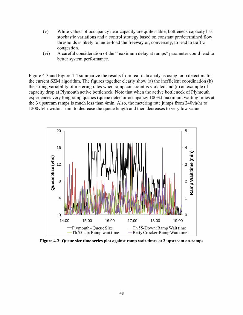
48

(v) While values of occupancy near capacity are quite stable, bottleneck capacity has stochastic variations and a control strategy based on constant predetermined flow thresholds is likely to under-load the freeway or, conversely, to lead to traffic congestion.

(vi) A careful consideration of the “maximum delay at ramps” parameter could lead to better system performance.

Figure 4-3 and Figure 4-4 summarize the results from real-data analysis using loop detectors for the current SZM algorithm. The figures together clearly show (a) the inefficient coordination (b) the strong variability of metering rates when ramp constraint is violated and (c) an example of capacity drop at Plymouth active bottleneck. Note that when the active bottleneck of Plymouth experiences very long ramp queues (queue detector occupancy 100%) maximum waiting times at the 3 upstream ramps is much less than 4min. Also, the metering rate jumps from 240vh/hr to 1200vh/hr within 1min to decrease the queue length and then decreases to very low value.

0

1

2

3

4

5

0

4

8

12

16

20

14:00 15:00 16:00 17:00 18:00 19:00

Ram

p W

ait t

ime

(min

)

Que

ue S

ize

(vhs

)

Plymouth - Queue Size Th 55-Down: Ramp Wait timeTh 55 Up: Ramp wait time Betty Crocker:Ramp Wait time

Figure 4-3: Queue size time series plot against ramp wait-times at 3 upstream on-ramps

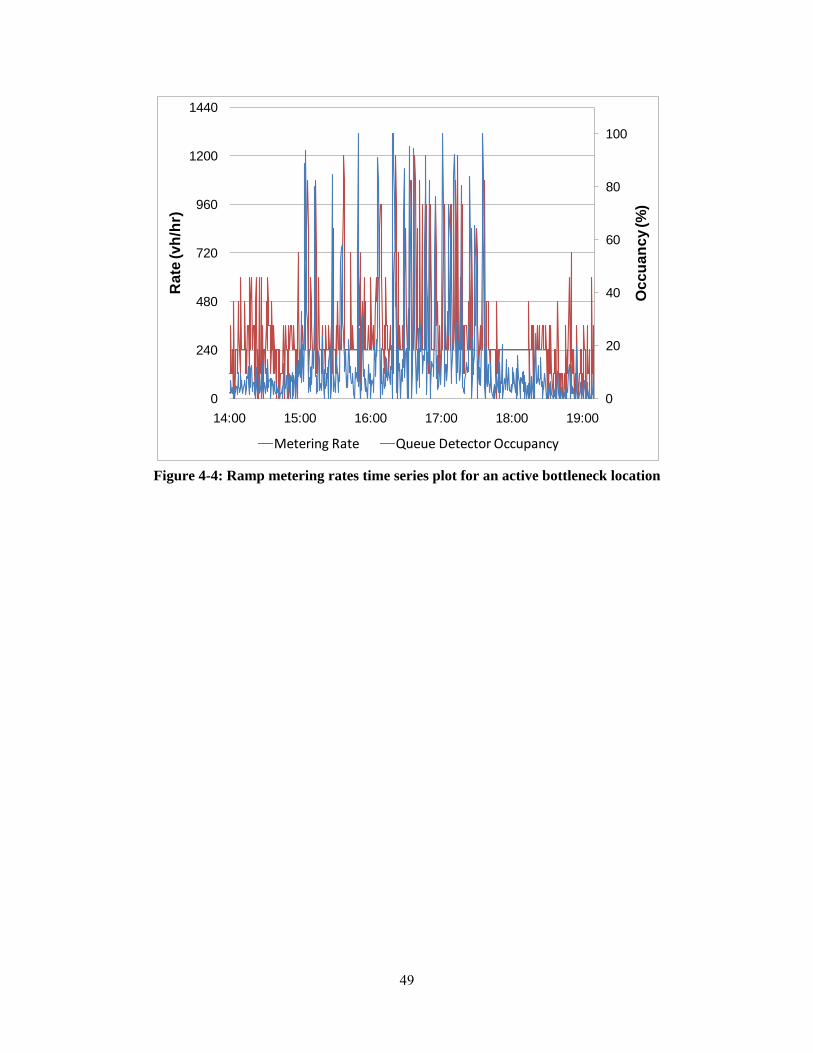
49

0

20

40

60

80

100

0

240

480

720

960

1200

1440

14:00 15:00 16:00 17:00 18:00 19:00

Occ

uanc

y (%

)

Rat

e (v

h/hr

)

Metering Rate Queue Detector Occupancy

Figure 4-4: Ramp metering rates time series plot for an active bottleneck location

50

51

Chapter 5 NEW RAMP METERING

Proposed Algorithm Instead of a layer-based algorithm as in the current SZM algorithm, we proceed with a dynamic zone definition based algorithm. The entire freeway system is divided into zones, where the length of each zone is dynamic and is estimated in real-time, i.e. it is embedded in the algorithm. Within each zone the metering rates are chosen independently of conditions in other zones. The zone boundaries and length mainly depend on (i) the level of congestion on the mainline direction, (ii) the demand and queue lengths at individual on-ramps and (iii) the location of the active bottleneck(s). An active bottleneck arises when vehicles discharge from an upstream queue (to guarantee that the bottleneck served vehicles at a maximum rate) and vehicles are unimpeded by traffic conditions emanating from further downstream of the location. The location of a recurring active freeway bottleneck is either (i) at freeway merges, where there is an additional inflow (ii) or in areas where the capacity changes (e.g. a change in topology from 3 to 2 lanes). Let us first define a section of a freeway. Section is (in most of the cases) a portion of the freeway between two consecutive mainline detector locations along the freeway. Each section usually contains one on-ramp and one off-ramp, with a few exceptions (e.g. freeway to freeway connections, two successive on-ramps etc). Each section cannot contain more than one on-ramps. This means that if there are more than one on-ramps between two consecutive mainline detectors, either the multiple on-ramps are in very close proximity and share merge lanes so that the ramps together are considered as a single on-ramp, or such a portion of the freeway is to be considered as consisting of x sections, where x is the number of on-ramps. When freeway traffic is free-flowing and on-ramp demands are low, coordinated metering strategy is not required and rates are estimated based on local conditions (effectively zone length equals one section). A coordinated algorithm is however used (effectively zone length > 1) when (i) there is a series of high demand ramps upstream of an active bottleneck or (ii) there are two closely spaced active bottlenecks and the downstream bottleneck is tending to propagate upstream. Thus, we need to provide the algorithm with procedures (i) for the identification of active bottlenecks in the freeway (ii) for choosing the appropriate type (local or coordinated) of control based on quantitative criterions and (iii) for estimating the boundaries and lengths of zones (starting section and ending section or zone length). We now provide the definition of a zone. A zone comprises an active bottleneck location (or a location which has a threat of becoming a potential active bottleneck if demand conditions continue as they are at a given point in time) at its downstream end and all upstream sections that are influenced by the bottleneck/threat. The associated on-ramp of this downstream bottleneck is the controlling ramp for this zone. All rates in the other ramps will be estimated towards postponing the occurrence of breakdown at the controlling ramp.

52

Each zone should tail off, if possible, with at least 2 sections with low on-ramp demands and which are known to be uncongested historically. This segmentation may lead to formation of long zones with more than one bottleneck locations within the zone. We will later address the issue of choosing the controlling ramp among different active bottlenecks. The objective of the algorithm is to keep vehicle density levels near all ramp locations below the congestion thresholds and to not allow occurrence of reduced speeds along the mainline, by constraining the ramp delays. The ramp rates are made to become stricter when the mainline density starts approaching the congestion threshold levels and the ramp rates are relaxed when the ramp waiting times approach the ramp delay threshold levels. Congestion on the freeway mainline is an undesirable condition. Equally as undesirable is a violation of the maximum ramp delay constraint since it results in having to increase the ramp rate enough to be able to disperse traffic, thus effectively once again threatening to cause breakdown on the freeway mainline. In situations where it no longer remains possible to keep both the freeway and the ramp in uncongested condition because of high on-ramp and mainline demands, the algorithm seeks to delay the violation of both the thresholds as much as possible. Thus the algorithm attempts to balance the congestions on the mainline and on the ramps so that occurrence of a breakdown on either is delayed as much as possible. The metering rates are consequently decided based on:

(i) Conditions on the freeway mainline a. How close the mainline density is to the density threshold (margin). b. How quickly the mainline density is approaching the density threshold (rate of

change). (ii) Conditions on the ramp

a. How close the current ramp delay on a ramp is to the threshold delay (margin). b. How fast the ramp delay is approaching the threshold delay (rate of change).

For example, in a hypothetical situation where two ramps have the same ramp delays, but these delays grow higher at different rates, the applied ramp flow rates should accordingly be different as well. In order to account for (i) the margin and (ii) the rate of change of the margin together for both, the ramps and the mainline sections, two key variables are introduced for each merge section. 𝑇𝑘 denotes the time duration available between the present and when the mainline density is expected to reach threshold values and thus approach congestion on mainline, provided the rate of change of density remains unchanged. Similarly, 𝑇𝑤 denotes the time duration available until the ramp delays reach their threshold levels. These estimates are used to define the current congestion level on the merge location and thus are used to decide the control mechanisms required. The congestion threat indices obtained for each merge location, are then used to: (i) identify locations for potential active bottlenecks, (ii) identify the severity of each potential bottleneck, and (iii) define zones as explained later. The zones are defined in such a way that the merge location at the downstream end of the zone is the most severe congestion threat and is thus deemed as the controlling bottleneck for the zone. The controlling bottleneck location continues to be metered in a manner so as to balance the congestions on the ramp and on the mainline, while all other merge locations within the zone are controlled in such a way that the ramp

53

violations be expected to occur simultaneously at all ramps within the zone. Since the zone and controlling bottleneck are identified in real-time, the algorithm is able to capture changes in demand patterns at different locations of the network and adapt accordingly.

Associated Variables and Parameters We first define the required variables for the development of the algorithm. The values of these variables are based on historical or real-time data from loop detectors. For each ramp i, we estimate the following variables, which are distinguished in historical and real-time variables. The first set of variables should be estimated before the implementation of the algorithm and are not time-dependent, while the second set of variables are dynamically estimated every 30sec. Note that all variables are estimated based on 30sec flow and density measures at a moving window of 5min moving averages every 30sec. This procedure smoothens random or unpredictable (difficult to estimate) phenomena such as short fluctuations in demand, variations in ratio of heavy axle vehicles in the sample of vehicles, detector errors, behavioral characteristics of drivers etc. Some of these variables have almost identical values among all ramps and in such cases global values are assigned. We also define some parameters, which are used to identify the different traffic states and decisions:

(1) Critical density on freeway mainline just upstream of ramp i, 𝑘𝑐𝑟𝑖𝑡(𝑖). This variable is used to identify the threshold between congested and uncongested conditions in the mainline. It is estimated from historic data as the average density among the 2% of the flow-density pairs observed for many days with the highest flow for the closest upstream detector to a merge. In most current algorithms of ramp metering based on density (e.g. ALINEA [33]) a slightly smaller value than the critical density is applied, e.g. 0.95×𝑘𝑐𝑟𝑖𝑡(𝑖). We also follow a similar approach.

(2) The capacity flow before and after the occurrence of congested conditions, 𝑐ℎ(𝑖)

and 𝑐𝑙(𝑖). 𝑐ℎ(𝑖) is estimated as the average flow from all the flow-density pairs with values of density between 0.95×𝑘𝑐𝑟𝑖𝑡(𝑖) and 1.00×𝑘𝑐𝑟𝑖𝑡(𝑖), while 𝑐𝑙(𝑖) for values of density between 1.00×𝑘𝑐𝑟𝑖𝑡(𝑖) and 1.05×𝑘𝑐𝑟𝑖𝑡(𝑖).

(3) The average density between the merge locations of the acceleration lane

associated with the ramp and the upstream mainline detector or 300 feet upstream whichever is shorter at time interval t. This estimation comes from the extended LWR density model as described in the earlier chapter (using finite differences of [25]). The LWR estimation is done using the internal boundaries along the freeway stretch, and accounts for the capacity drop phenomenon at each location. The length to be used can also be overwritten for special cases. The rate of change of the mainline density for an interval with duration 𝑇 is then calculated as:

𝛥𝑘𝑡(𝑖) = [𝑘𝑡(𝑖) − 𝑘𝑡−1(𝑖) ] / 𝑇 (6) (4) The maximum waiting time for vehicles on the ramp at interval t (based on a

combination of arrival and departure patterns and on occupancy of queue

54

detectors), 𝑤𝑡(𝑖). The rate of change of the delay for the ramps is then calculated as

𝛥𝑤𝑡(𝑖) = [𝑤𝑡(𝑖) − 𝑤𝑡−1(𝑖) ] / 𝑇 (7) (5) The time duration until the occurrence of congested conditions on the mainline,

i.e. time-to-congestion on mainline is estimated as 𝑇𝑡𝑘(𝑖) = (𝑘𝑐𝑟𝑖𝑡(𝑖) − 𝑘𝑡(𝑖))/𝛥𝑘𝑡(𝑖) (8)

(6) The time duration until the violation of ramp wait time constraint 𝑇𝑐𝑟𝑖𝑡, i.e. time-

to-ramp-congestion is estimated as

𝑇𝑡𝑤(𝑖) = [𝑇𝑐𝑟𝑖𝑡 – 𝑤𝑡(𝑖)] / 𝛥𝑤𝑡(𝑖) (9) We next assign the state conditions for each merge location. The state conditions define the potential threat of a bottleneck being formed at a given location. A 0-state is assigned to a location expected to pose minimal threat as a bottleneck at the current time, 1-state is given to a location approaching congestion state while still under the threshold level, while a location assigned the 2-state level is already in the completely congested regime. These states contribute towards the estimation of zone lengths and the type of ramp metering employed at the location (local or coordinated). State 0 occurs when mainline density is small, and time-to-congestion is large for both mainline and ramp. State 1 occurs when mainline density is medium and time-to-congestion is positive for both mainline and ramp yet small for at-least one, while state 2 occurs when congestion is already being observed on the mainline or on the ramp, i.e. 𝑇𝑡𝑘(𝑖) or 𝑇𝑡𝑤(𝑖) is negative. State 1 merge locations are distinguished from State 0 conditions so that in absence of any stronger (state 2) locations in the neighborhood, a state 1 location may be assumed as the controlling bottleneck and control strategy make efforts towards either averting or delaying the conversion of this state 1 into a state 2 location. The different states, 𝑆𝑡(𝑖), at each merge location are identified as follows (where δ, 𝜏𝑘 and 𝜏𝑤 are thresholds to quantitatively distinguish between states; δ is a low density margin for the mainline to separate state 0 from 1, e.g. 70-80% of critical density; 𝜏𝑘 for mainline and 𝜏𝑤 for ramps are the safe time intervals before the mainline (or the ramp) are considered to be under risk of being congested (or overflow), e.g. 10min):

𝑆𝑡(𝑖) = �𝑡 𝑐𝑟𝑖𝑡 𝑡

𝑤𝑤 𝑡

𝑘𝑘

2, 𝑖𝑓 [𝑇𝑡𝑘(𝑖) < 0 ] 𝑂𝑅 [ 𝑇𝑡𝑤(𝑖) < 0 ] (10) 0, 𝑖𝑓 [ 𝑘 (𝑖) < 𝛿 × 𝑘 (𝑖) ] 𝐴𝑁𝐷 [ 𝑇 (𝑖) > 𝜏 ] 𝐴𝑁𝐷 [ 𝑇 (𝑖) > 𝜏 ]

1, 𝑜𝑡ℎ𝑒𝑟𝑤𝑖𝑠𝑒.

�

When there exist 2 problematic locations close to congestion thresholds which are in the same neighborhood (2-3 sections apart), the algorithm needs to choose and decide which location needs to be treated as the controlling section. There are 2 options:

55

a. If the upstream location experiences more severe demand conditions, then the freeway is separated into two zones, one ending at the upstream location and another one between the two problematic locations.

b. If the downstream location experiences more severe demand conditions, then there is only one zone for this freeway and the controlling ramp is the downstream one. All ramp rates are estimated with respect to the controlling location and as explained before the goal is that all ramps reach the ramp waiting constraint simultaneously.

To identify the most problematic location, we define the net inflow between the two locations i and j, 𝑀𝑡(𝑖, 𝑗), given as the sum of on-ramp volumes minus the sum of off-ramp volumes for all ramps between the two locations. This justifies whether the demand at the upstream problematic location is higher or lower than demand at the downstream location, thus representing the gain of vehicles within the given section for the specified interval. This variable will help in choosing the critical bottleneck, which will define the metering rates in the coordinated strategy. The zone decision criterion ensures realization of the highest possible overall throughput, by either avoiding the bottleneck to affect a high exit / low input location downstream of the real threat location, or by ensuring that only a single bottleneck is formed (at the downstream location), rather than the possibility of formation of 2 individual threats thus also adversely affecting exits between the locations. If capacities of the two sections are different we account for this by adding the loss in capacity from the net input obtained from the ramp flows. Thus the net inflow is (𝐼𝑡𝑘 and 𝑂𝑡𝑘 is the on-ramp and off-ramp flow associated with section k at time t)

𝑀𝑡 𝑡𝑘

𝑡𝑘 ℎ ℎ (𝑖, 𝑗) = �𝐼 − 𝑂

𝑗

𝑖

+ 𝑐 (𝑖) − 𝑐 (𝑗) (11)

Bottleneck and Zone Identification The state conditions identify the problematic locations that can be expected to become the active bottleneck(s). The zone identifies the associated sequence of sections that get affected by a given active bottleneck (or are expected to get affected by a potential active bottleneck before it is actually formed). Thus, the definition of zones also relies on the identification of the active bottleneck locations and threats. Usually a zone would have congested / near congested location(s) at its downstream end and 2-3 uncongested sections at the upstream end. To identify the controlling ramps and the zone length when conditions are near or at congestion, we start from the most downstream location of the freeway and move upstream by analyzing each location individually at each step. We then use the following rules to mark a merge as the controlling location. Each zone has only one controlling section/ramp at its downstream end and all the upstream ramp rates are calculated as a function of the controlling one. For clarity, we adopt a naming convention for the sections such that the sections are numbered from 1 to N (N being the total number of sections along the freeway) starting at the downstream end of the stretch (section j has section j-1 located immediately downstream of itself). We then first estimate the state of all sections, 𝑆𝑡(𝑗) for all j=1, 2, 3… N, as defined in equation 11. Once the bottleneck threat state levels are defined for the sections, we then define the controlling

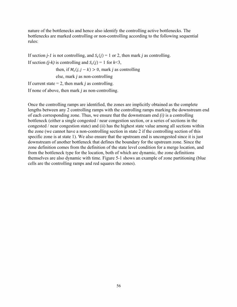
56

nature of the bottlenecks and hence also identify the controlling active bottlenecks. The bottlenecks are marked controlling or non-controlling according to the following sequential rules: If section j-1 is not controlling, and 𝑆𝑡(𝑗) = 1 or 2, then mark j as controlling. If section (j-k) is controlling and 𝑆𝑡(𝑗) = 1 for k<3, then, if 𝑀𝑡(𝑗, 𝑗 − 𝑘) > 0, mark j as controlling else, mark j as non-controlling If current state = 2, then mark j as controlling. If none of above, then mark j as non-controlling. Once the controlling ramps are identified, the zones are implicitly obtained as the complete lengths between any 2 controlling ramps with the controlling ramps marking the downstream end of each corresponding zone. Thus, we ensure that the downstream end (i) is a controlling bottleneck (either a single congested / near congestion section, or a series of sections in the congested / near congestion state) and (ii) has the highest state value among all sections within the zone (we cannot have a non-controlling section in state 2 if the controlling section of this specific zone is at state 1). We also ensure that the upstream end is uncongested since it is just downstream of another bottleneck that defines the boundary for the upstream zone. Since the zone definition comes from the definition of the state level condition for a merge location, and from the bottleneck type for the location, both of which are dynamic, the zone definitions themselves are also dynamic with time. Figure 5-1 shows an example of zone partitioning (blue cells are the controlling ramps and red squares the zones).

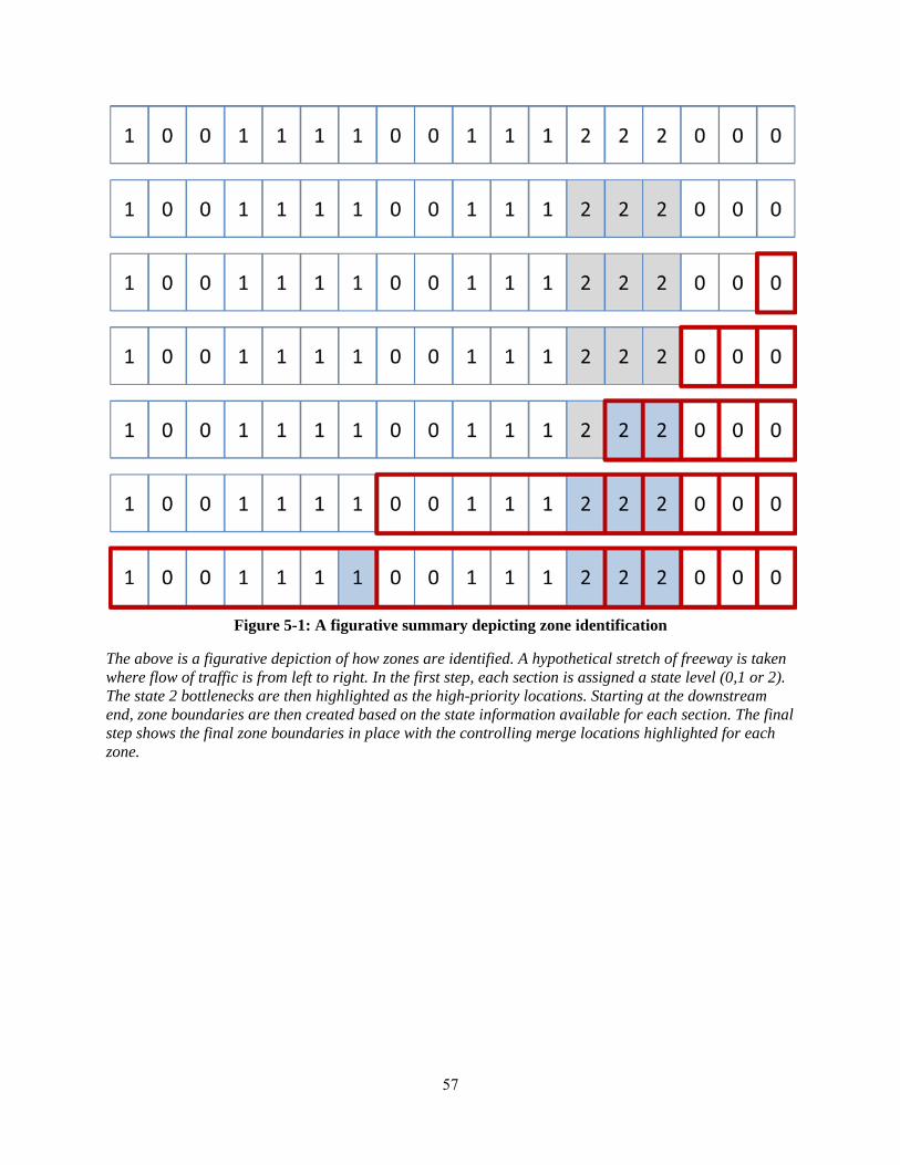
57

Figure 5-1: A figurative summary depicting zone identification

The above is a figurative depiction of how zones are identified. A hypothetical stretch of freeway is taken where flow of traffic is from left to right. In the first step, each section is assigned a state level (0,1 or 2). The state 2 bottlenecks are then highlighted as the high-priority locations. Starting at the downstream end, zone boundaries are then created based on the state information available for each section. The final step shows the final zone boundaries in place with the controlling merge locations highlighted for each zone.

58

Action Matrix Given the zone identification, the metering actions are then governed for each zone by the state of the various ramp locations and controlling bottlenecks within the zone. We first decide the control action employed as defined by the following rules (Each control action is explained later in better detail):

1. State = 0, downstream controlling ramp = no, (zone length z = 1) Uncongested Ramp Metering For merge location in state 0, with no controlling ramp present downstream of the current

merge location within the same zone, an isolated ramp metering strategy is applied. Since the location is considered isolated from any other merge location and from the influence of any bottleneck, the metering rate locally applied tries to maintain the total input flows from the mainline upstream of the location, and from the ramp, under the known capacity for the section.

2. State = 0/1, downstream controlling ramp = yes, (z>1) Controlled Ramp Metering Any merge location marked as state 0 or state 1, that have a presence of an active

controlling ramp downstream of their location within the zone, the merge location is considered to be under controlled metering requirement where the metering control is applied towards improving the threat condition at the downstream controlling ramp location. Since the current ramp itself does not pose a bigger threat than the downstream location in the given case, the downstream threat is prioritized.

3. State = 1, downstream controlling ramp = no Controlling Ramp Metering Any merge location marked as state 1, with no present controlling ramp downstream

within the zone, is boosted in priority to a controlling level since the ramp itself becomes the most threatening location within its neighborhood. This ramp now acts as the controlling ramp for all the upstream ramps with the same zone. The ramp however, cannot act as the controlling ramp for an upstream location that is a bigger threat (is in state 2) and such cases are automatically handled during zone definition with the state 2 upstream location marking the start of a new zone.

4. State = 2 Congested Ramp Metering Any merge location marked as state 2, is given highest stage of priority. Such a both acts

as the defining boundary for a zone (since no downstream location can take precedence of it), and as the dominating merge location for all upstream locations within the zone. The merge location marked as state 2 is controlled effectively in an isolated manner and works towards improving the conditions on the present location.

59

Figure 5-2 shows a graphical description of the metering strategy decision making process based on the bottleneck severity information and the zone definitions.

Figure 5-2: Assignment of control strategies following zone identification

Where the above defines briefly the various control strategies employed for the various scenarios and conditions along with the ideologies involved, we next explain these control strategies in more detail.

1. Uncongested Metering Uncongested Metering is an isolated control mechanism where the current ramp location is metered in a way so as to try and keep the conditions uncongested and avoid over-loading the associated mainline section. This strategy is applied to locations that are neither congestion threats themselves, nor are they under the influence of any other nearby bottleneck threats. Controlling these merge locations is expected to not have any effect on other bottleneck threats in the vicinity. The metering rate employed is aimed at ensuring that the overall demand on associated section (freeway demand + ramp demand) does not exceed the uncongested capacity at the section. Although any simple isolated strategy can be employed at such locations (e.g. ALINEA), we suggest the simplest method for calculating the metering rate as:

𝑟𝑡(𝑖) = 𝑐ℎ(𝑖) − 𝑞𝑡(𝑖) (12) where, is the metering rate at the ramp, is the uncongested capacity, and is the mainline flow upstream of the merge, or the mainline demand at the location.

2. Controlled Metering

Controlled Metering is a coordinated metering mechanism where the merge location under controlled metering is controlled in a way such as to work towards improving the conditions at the controlling merge location downstream of itself but within the same

𝑟𝑡(𝑖) 𝑐ℎ(𝑖) 𝑞𝑡(𝑖)

60

zone. The merge location under controlled metering is either in an uncongested safe state 0, or in a approaching congestion state 1 and is not itself under congested regime. The metering at such locations is done towards an aim of balancing the ramp delays at the current location with the ramp delays experienced at the controlling ramp location. In doing so, a balanced state is achieved between the controlling ramp and a series of all controlled ramps that belong to the zone. The series of all controlled ramps affected is also the set of all ramps that are expected to be able to help towards improving conditions at the controlling merge location. The end goal is to be able to monitor metering rates at all the affected locations so that all such ramps approach towards their respective ramp wait time constraints simultaneously. The following formulation guarantees such a behavior:

𝑟𝑡(𝑖) = 𝑑𝑖 −Δti i j t

∗ d �d − r (j)�Δtjdj

, (13)

wher

𝑤

e,

(𝑖)

is the demand and 𝑖

is𝑐

th𝑟𝑖𝑡

e mete𝑡

ring rate at 𝑐

ra𝑟𝑖𝑡

mp i, j is the bottleneck location or the c

𝑡

ontrolling ramp and , where is the ramp delay constraint and is the current maximum wait experienced at ramp i.

3. Controlling Metering

Controlling Metering is applied at merge locations that are not under the influence of any other downstream congestion threats but are themselves approaching congestion and thus need to be monitored. The controlling merge locations also define the rate at which the associated controlled merges are metered. The objective of the controlling metering strategy is to try postponing the occurrence of congestion at the present location as much as possible. The controlling metering strategy works towards delaying congestion on both the freeway and the ramp. The objective is achieved by balancing the approach of congestion on the mainline with the approach of the violation of ramp wait time constraint (as indicator of congestion) on the corresponding ramp. Thus, metering is tightened when mainline starts approaching congestion quicker than ramp congestion, and loosened when the ramp approaches congestion faster than the mainline does. The metering rate is decided based on the following formulation:

𝑟𝑡(𝑖) = 𝑟𝑡−1(𝑖) − 𝐾1( 𝑇𝑡𝑤(𝑖) − 𝜏𝑤) + 𝐾2𝑇𝑡𝑘(𝑖) (14) w

𝑇𝑤

h

(

er

𝑖)

e

and are contribution parameters that are used to define the importance of br𝑡

eakdown on ram

𝜏

p a

nd on mainline respectively (units as vehicles / min2), and are the estim

𝑤

ated time remaining till congestion sets in on the mainline an𝑘

d ramp respectively, and is the safe time-to-breakdown defined for the ramp.

𝑡

4. Congested Metering Any merge location under state 2 automatically enters the congested metering control strategy. Such a location can also prove to be the controlling bottleneck location for upstream controlled locations, but is itself monitored different from a controlling metering strategy. A location in state 2 is already under congestion, either on the mainline, or on the ramp, or on both. The priority is given to the violation threat on the ramp. Under case where the ramp is congested or the delay times on ramp have already

𝐾1 𝐾2 𝑇 (𝑖)

𝑑𝑖 𝑟𝑡(𝑖) 𝛥𝑡 = 𝑇 − 𝑤 (𝑖) 𝑇

61

exceeded the wait time constraints, the metering rate is increased progressively till a balance is reached that ‘just’ avoids further ramp wait time constraint violations. In case where the ramp congestion has not yet been observed, the metering rate is decreased progressively in order to improve the conditions on the mainline. The formulation for deciding the ramp metering rate can thus be defined as:

𝑖𝑓 [𝑇𝑡𝑤(𝑖) < 0] 𝑡ℎ𝑒𝑛 𝑟𝑡(𝑖) = 𝑟𝑡−1(𝑖) + 𝐾1𝑇𝑡𝑤(𝑖) 𝑒𝑙𝑠𝑒, 𝑟𝑡(𝑖) = 𝑟𝑡−1(𝑖) + 𝐾2 ∗ 𝑇𝑡𝑘(𝑖) (15)

where the variables used have the same meanings as in the previous control strategy formulations. To avoid rapid increases in the metering rates (rapid fluctuations in metering rate is observed as a draw

𝑇

ba

𝑤

c

(𝑖

k

)

plaguing ma𝑎ny curren

𝑇t𝑡𝑤 a

(lgor𝑖)

ithms like SZM), we define a maximum change of

𝑡

metgood estimator of

𝑤

𝑟 (𝑖) − 𝑟

𝐾

er

1𝑇

ing vais n

𝑡

o

lue , when <0t easily obtainable when

𝑎

, so that 𝑡 𝑡−1 . As a the queue detector remains near-

continuously occupied, can be used in place of .

(𝑖) < 𝑎

The metering rates as obtained through the above control strategies provide the target metering rates for all the ramp access locations along the freeway network. These rates can then be rounded off into pre-defined slots of metering rates so that an operational and balanced rate is decided. The metering strategy in its entirety is a mix of isolated and coordinated control strategies and is based on real time dynamic definitions of zones based on traffic conditions at the various merge locations and their corresponding mainline sections. While all controlled locations within a zone are metered in a coordinated manner so as the relieve stress at the most threatening bottleneck in the vicinity, isolated locations use local control mechanisms. Metering is done with an objective of balancing stresses on the mainline and the ramps at bottleneck locations, and balancing congestion threats on all coordinated ramps within zones.

Application and Results

Test Site and Input Data The developed metering strategy is tested through AIMSUN micro-simulator in a 12-mi segment of Trunk Highway 169 northbound (TH-169 NB), starting from the I-494 interchange and ending at 63rd Avenue North. This site is a circumferential freeway traversing the Twin Cities west metropolitan region. It includes 10 weaving sections, 4 HOV bypass ramps, 24 entrance ramps (17 metered), and 25 exit ramps. Among the metered ramps, 15 local access ramps and two freeway-to-freeway ramps connect TH-62 and I-394, respectively. The upstream and downstream boundaries are uncongested. The test site is a larger extension of the site most extensively used for the bottleneck analysis portion of this report. The 15-min-interval traffic demand data used in the simulation were extracted from the Minnesota DOT loop detector database. For the purpose of this study, only one peak period was tested, specifically the p.m. peak on September 25, 2008 between 2pm and 8pm. Figure 5-3 summarizes the demand for a subset of the on-ramps of the study site.

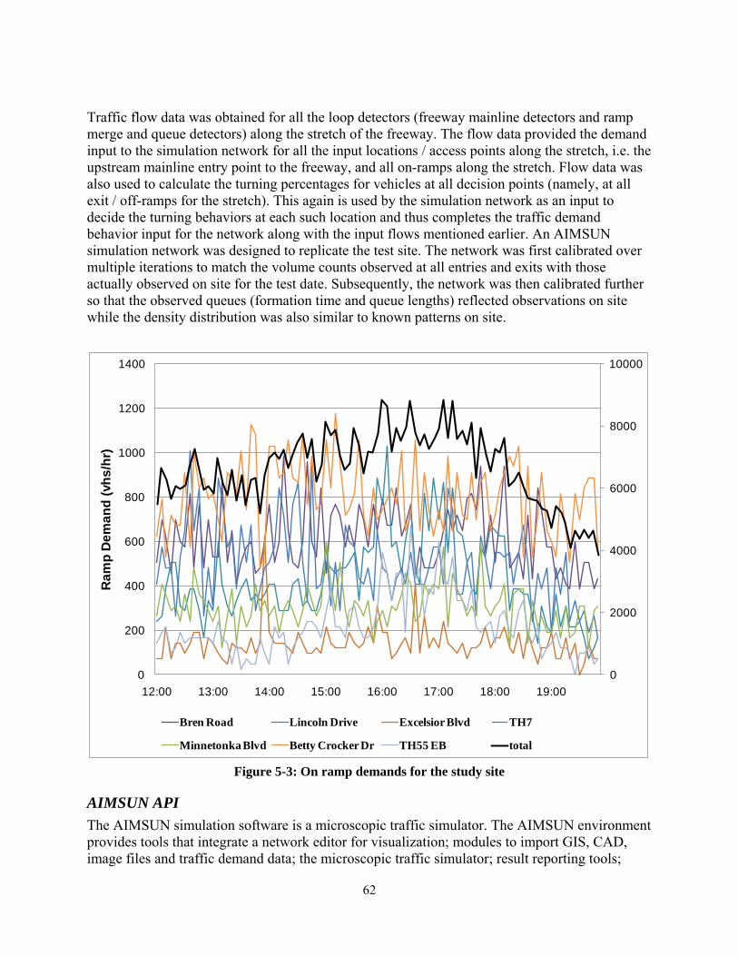
62

Traffic flow data was obtained for all the loop detectors (freeway mainline detectors and ramp merge and queue detectors) along the stretch of the freeway. The flow data provided the demand input to the simulation network for all the input locations / access points along the stretch, i.e. the upstream mainline entry point to the freeway, and all on-ramps along the stretch. Flow data was also used to calculate the turning percentages for vehicles at all decision points (namely, at all exit / off-ramps for the stretch). This again is used by the simulation network as an input to decide the turning behaviors at each such location and thus completes the traffic demand behavior input for the network along with the input flows mentioned earlier. An AIMSUN simulation network was designed to replicate the test site. The network was first calibrated over multiple iterations to match the volume counts observed at all entries and exits with those actually observed on site for the test date. Subsequently, the network was then calibrated further so that the observed queues (formation time and queue lengths) reflected observations on site while the density distribution was also similar to known patterns on site.

0

2000

4000

6000

8000

10000

0

200

400

600

800

1000

1200

1400

12:00 13:00 14:00 15:00 16:00 17:00 18:00 19:00

Ram

p D

eman

d (v

hs/h

r)

Bren Road Lincoln Drive Excelsior Blvd TH7

Minnetonka Blvd Betty Crocker Dr TH55 EB total

Figure 5-3: On ramp demands for the study site

AIMSUN API The AIMSUN simulation software is a microscopic traffic simulator. The AIMSUN environment provides tools that integrate a network editor for visualization; modules to import GIS, CAD, image files and traffic demand data; the microscopic traffic simulator; result reporting tools;

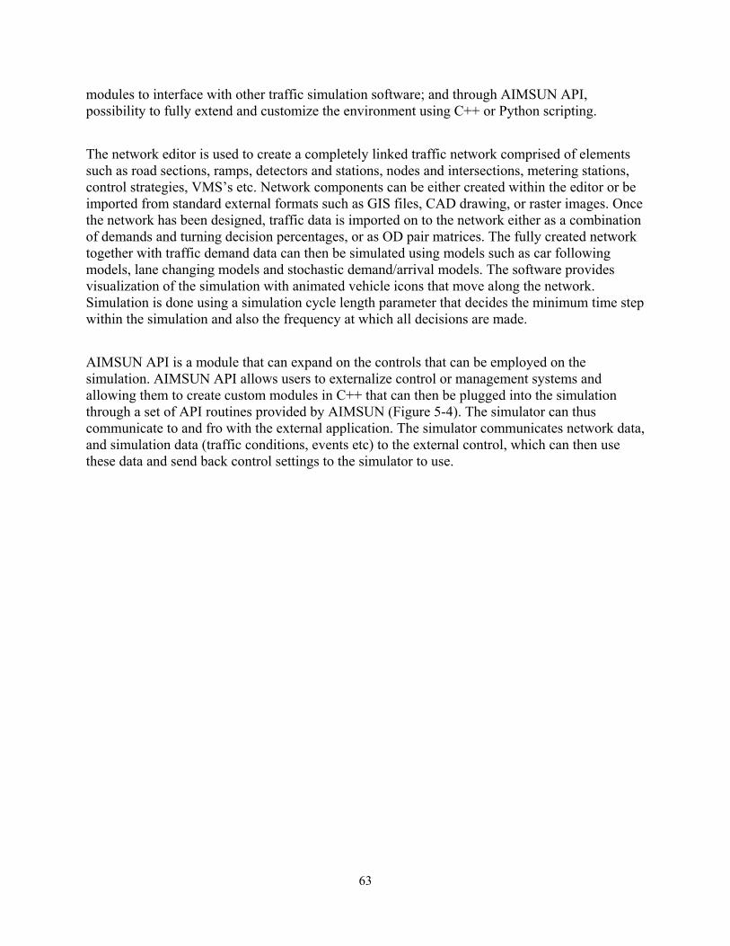
63

modules to interface with other traffic simulation software; and through AIMSUN API, possibility to fully extend and customize the environment using C++ or Python scripting. The network editor is used to create a completely linked traffic network comprised of elements such as road sections, ramps, detectors and stations, nodes and intersections, metering stations, control strategies, VMS’s etc. Network components can be either created within the editor or be imported from standard external formats such as GIS files, CAD drawing, or raster images. Once the network has been designed, traffic data is imported on to the network either as a combination of demands and turning decision percentages, or as OD pair matrices. The fully created network together with traffic demand data can then be simulated using models such as car following models, lane changing models and stochastic demand/arrival models. The software provides visualization of the simulation with animated vehicle icons that move along the network. Simulation is done using a simulation cycle length parameter that decides the minimum time step within the simulation and also the frequency at which all decisions are made. AIMSUN API is a module that can expand on the controls that can be employed on the simulation. AIMSUN API allows users to externalize control or management systems and allowing them to create custom modules in C++ that can then be plugged into the simulation through a set of API routines provided by AIMSUN (Figure 5-4). The simulator can thus communicate to and fro with the external application. The simulator communicates network data, and simulation data (traffic conditions, events etc) to the external control, which can then use these data and send back control settings to the simulator to use.

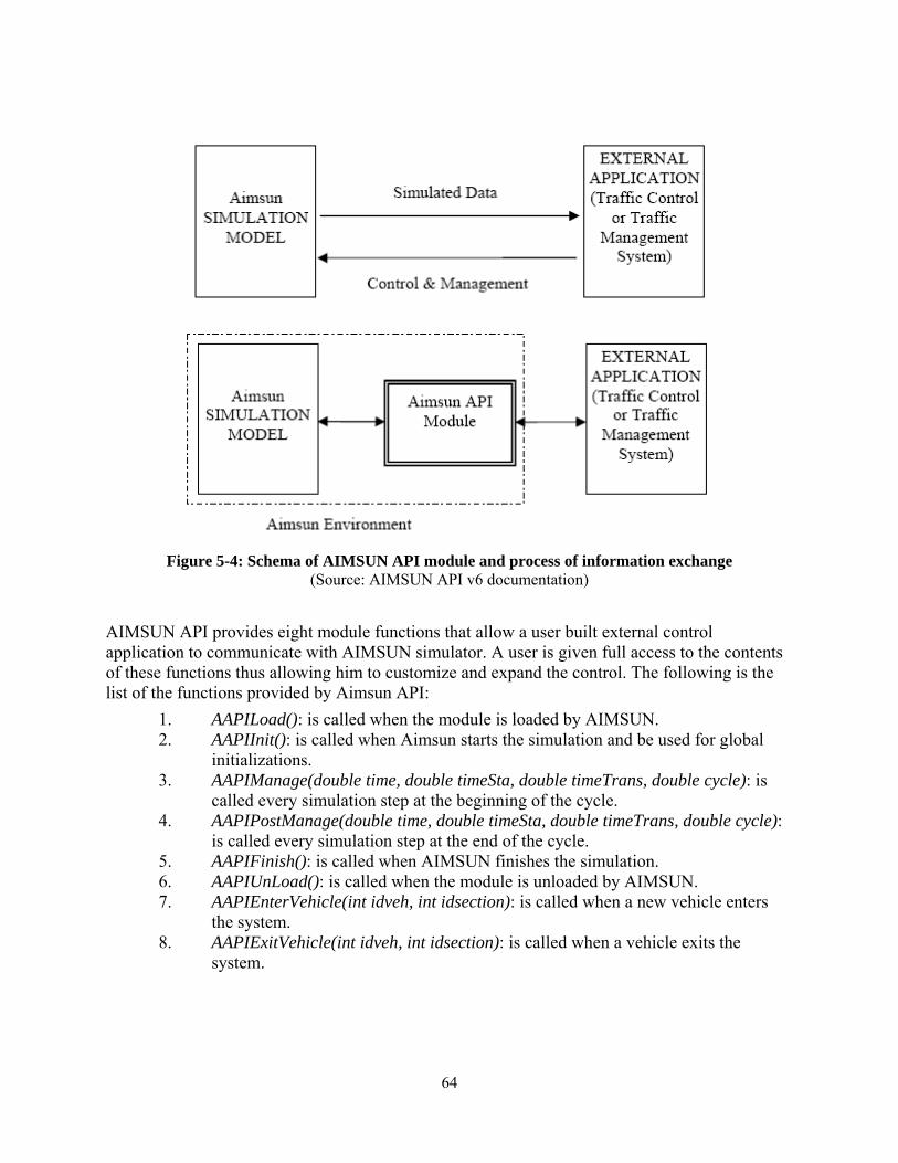
64

Figure 5-4: Schema of AIMSUN API module and process of information exchange

(Source: AIMSUN API v6 documentation)

AIMSUN API provides eight module functions that allow a user built external control application to communicate with AIMSUN simulator. A user is given full access to the contents of these functions thus allowing him to customize and expand the control. The following is the list of the functions provided by Aimsun API:

1. AAPILoad(): is called when the module is loaded by AIMSUN. 2. AAPIInit(): is called when Aimsun starts the simulation and be used for global

initializations. 3. AAPIManage(double time, double timeSta, double timeTrans, double cycle): is

called every simulation step at the beginning of the cycle. 4. AAPIPostManage(double time, double timeSta, double timeTrans, double cycle):

is called every simulation step at the end of the cycle. 5. AAPIFinish(): is called when AIMSUN finishes the simulation. 6. AAPIUnLoad(): is called when the module is unloaded by AIMSUN. 7. AAPIEnterVehicle(int idveh, int idsection): is called when a new vehicle enters

the system. 8. AAPIExitVehicle(int idveh, int idsection): is called when a vehicle exits the

system.

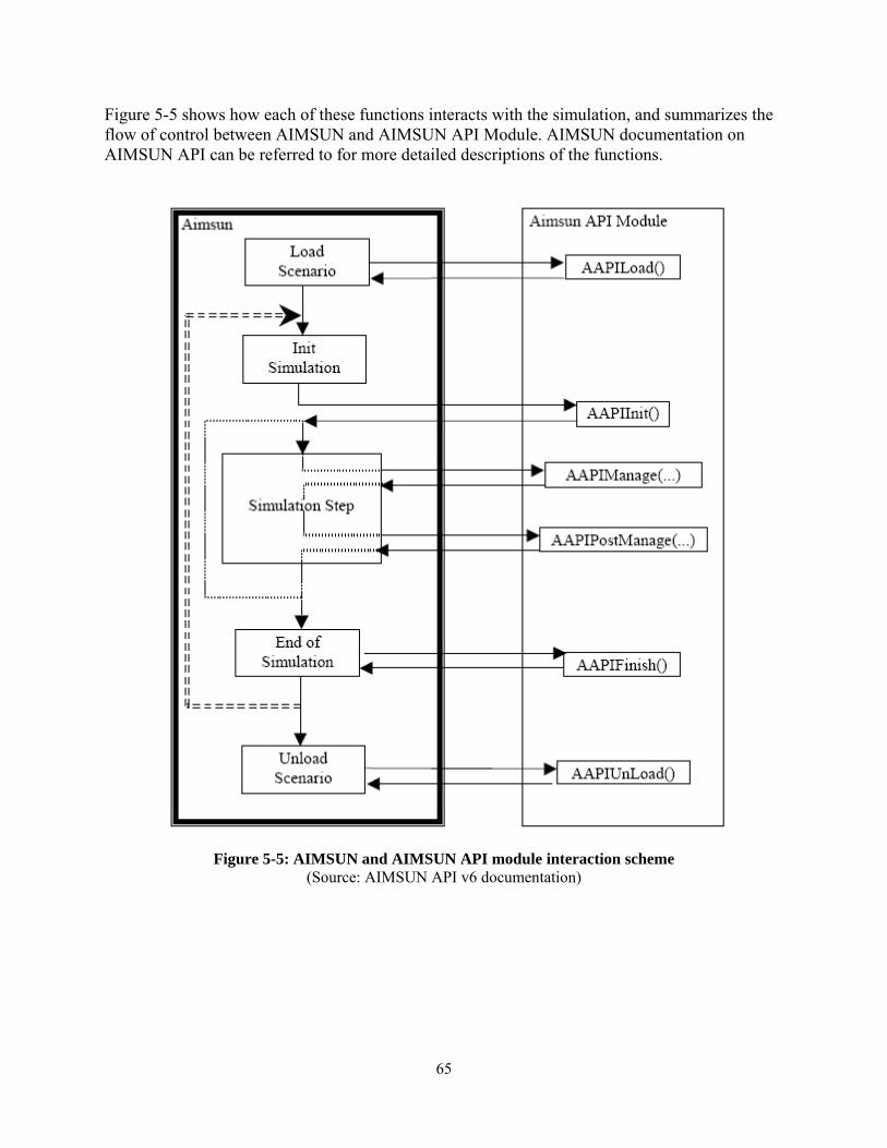
65

Figure 5-5 shows how each of these functions interacts with the simulation, and summarizes the flow of control between AIMSUN and AIMSUN API Module. AIMSUN documentation on AIMSUN API can be referred to for more detailed descriptions of the functions.

Figure 5-5: AIMSUN and AIMSUN API module interaction scheme

(Source: AIMSUN API v6 documentation)

66

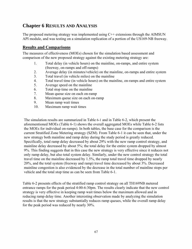
67

Chapter 6 RESULTS AND ANALYSIS

The proposed metering strategy was implemented using C++ extensions through the AIMSUN API module, and was testing on a simulation replication of a portion of the US169-NB freeway.

Results and Comparisons The measures of effectiveness (MOEs) chosen for the simulation based assessment and comparison of the new proposed strategy against the existing metering strategy are:

1. Total delay (in vehicle hours) on the mainline, on-ramps, and entire system (freeway, on-ramps and off-ramps)

2. Average delay (in minutes/vehicle) on the mainline, on-ramps and entire system 3. Total travel (in vehicle miles) on the mainline 4. Total travel time (in vehicle hours) on the mainline, on-ramps and entire system 5. Average speed on the mainline 6. Total stop time on the mainline 7. Mean queue size on each on-ramp 8. Maximum queue size on each on-ramp 9. Mean ramp wait times 10. Maximum ramp wait times

The simulation results are summarized in Table 6-1 and in Table 6-2, which present the aforementioned MOEs (Table 6-1) shows the overall aggregated MOEs while Table 6-2 lists the MOEs for individual on-ramps). In both tables, the base case for the comparison is the current Stratified Zone Metering strategy (SZM). From Table 6-1 it can be seen that, under the new strategy both mainline and ramp delay during the study period is greatly reduced. Specifically, total ramp delay decreased by about 29% with the new ramp control strategy, and mainline delay decreased by about 5%; the total delay for the entire system dropped by almost 9%. This finding suggests that in this case the new strategy is very effective since it reduces not only ramp delay, but also total system delay. Similarly, under the new control strategy the total travel time on the mainline decreased by 1.5%, the ramp total travel time dropped by nearly 20%, and the total system (freeway and ramp) travel time decreased by about 3%. Decreased mainline congestion is also evidenced by the decrease in the total number of mainline stops per vehicle and the total stop time as can be seen from Table 6-1.

Table 6-2 presents effects of the stratified ramp control strategy on all TH169NB metered entrance ramps for the peak period 4:00-6:30pm. The results clearly indicate that the new control strategy is very effective in keeping ramp wait times below the maximum allowed and in reducing ramp delay time. Another interesting observation made by analyzing the simulation results is that the new strategy substantially reduces ramp queues, while the overall ramp delay for the peak period was reduced by nearly 30%.

68

Table 6-1: Network MOEs for SZM and new metering (Sep 25, 2008, 2:00pm-8:00pm)

Mainline 5692 5605 -1.53%Ramp 430 341 -20.63%Entire Site 6164 5980 -2.99%

Total Travel veh-mi Entire Site 290187 288864 NAMainline 1427 1359 -4.77%Ramp 276 196 -29.01%Entire Site 1714 1566 -8.64%Mainline 1.27 1.26 -0.79%Ramp 0.39 0.28 -28.21%Entire Site 1.66 1.54 -7.23%

Total Stop Time veh-hrs Mainline 181 159 -12.15%Speed mph Mainline 54.69 54.79 0.18%

SZM New MeteringPerc Incr over

SZM

Total Travel Time

PERFORMANCE MEASURES

veh-hrs

Total Delay

Average Delay min/veh

veh-hrs

Table 6-2: Ramp MOEs during peak period (Sep 25, 2008, 4:00pm-6:30pm)

Ramp SZM New SZM New SZM New SZM New SZM New

Valley View 0.29 0.43 1.65 1.43 8.78 13.10 2 3 12 17TH 62 0.50 0.68 2.12 5.03 29.23 39.59 4 5 25 27Bren Road 0.86 1.06 4.51 3.88 24.42 30.11 5 6 24 30Lincoln Drive 0.43 0.07 1.10 0.52 2.77 0.45 3 1 7 1Excelsior Blvd 0.73 0.22 3.47 0.82 16.89 4.99 4 1 25 8TH7 0.14 0.17 1.56 0.63 3.48 4.35 3 1 15 736th Street 0.29 0.07 2.00 0.10 3.84 0.91 2 1 11 1Minnetonka Blvd 0.27 0.07 2.33 0.23 2.61 0.70 2 1 9 1I-394 3.66 1.82 3.75 2.55 19.04 9.49 3 1 13 5Betty Crocker Dr 0.56 0.52 4.00 4.10 9.02 8.38 5 2 18 21TH55 0.51 0.12 4.06 0.70 12.32 2.91 3 1 13 5Plymouth Ave 1.29 0.07 4.10 0.37 20.83 1.12 5 1 17 6Medicine Lake Rd 1.11 0.12 4.29 0.50 12.17 1.30 3 1 20 5TOTAL 165.39 117.41

Avg Ramp Delay Max Ramp Wait Average Queue Size Maximum Queue4:00 - 6:30 Total Ramp Delay(minutes) (minutes) (vehicle-hours) (vehicles) (vehicles)

A simple sensitivity analysis was carried out on the parameter that indicates the ramp constraint wait times for all the ramps. For the original reported results (Table 6-1 and Table 6-2), ramp constraint wait times for all ramps along the network was set to being 4 minutes (recommended value used by Mn/DOT) while the constraint was relaxed at the TH62 ramp, that reported highest delays on ramp in simulation, to 5 minutes. For the sensitivity analysis, simulation runs were made first for varying allowable ramp delay constraints on all ramps while keeping the delay constraint constant for TH62 ramp. Table 6-3 lists the system MOEs obtained for this set of test cases. Similarly, a set of simulation runs were also made for varying values of delay constraint on the TH62 ramp while keeping all other ramps constant, with Table 6-4 listing the resulting MOEs for the cases. From both the test sets, we see that the ramp

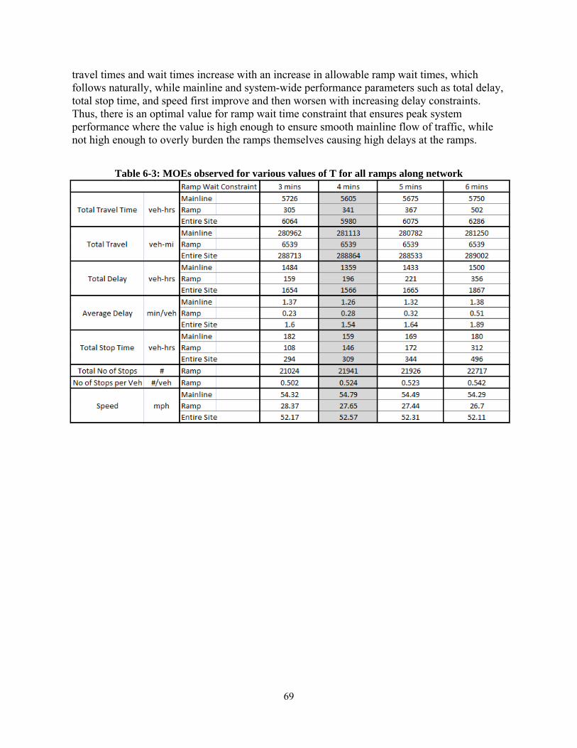
69

travel times and wait times increase with an increase in allowable ramp wait times, which follows naturally, while mainline and system-wide performance parameters such as total delay, total stop time, and speed first improve and then worsen with increasing delay constraints. Thus, there is an optimal value for ramp wait time constraint that ensures peak system performance where the value is high enough to ensure smooth mainline flow of traffic, while not high enough to overly burden the ramps themselves causing high delays at the ramps.

Table 6-3: MOEs observed for various values of T for all ramps along network

70

Table 6-4: MOEs observed for various values of T for TH62 ramp

71

Conclusions The project was designed in order to explore development of a density based ramp metering algorithm to replace the currently deployed Stratified Zone Metering algorithm on Minnesota’s freeways. The decision to use density-based metering as opposed to the more commonly used flow measure based metering was motivated by empirical results indicating (i) that the recurrent traffic breakdown can occur at different capacity values, even under the same operating conditions and (ii) critical density value for this stochastic capacity is more stable. The proposed metering algorithm was expected to show improvements in average delays on the system over the SZM algorithm. The development of the algorithm was done in a two-phase manner. Various bottlenecks were studied to understand breakdown behavior and the reaction of traffic states to metering patterns. This was presented in the first portion of this report. A coordinated metering strategy was then developed based on the findings of these studies. The metering strategy dynamically assesses conditions on mainline and ramps and decides the threat of occurrence of congestion at each iteration. This information is then used to define a zone of effect for each bottleneck threat location. The ramps within a zone are then metered based on a set of rules aiming at reducing the load on the bottleneck threat location in a coordinated manner so that all ramps approach congestion at similar rates. The proposed algorithm was developed and deployed on AIMSUN traffic simulator. Various traffic MOEs were used to assess the performance of the new algorithm on the simulated network, and the algorithm was compared to the performance of the SZM strategy. The test results indicate that the density-based feedback coordinated algorithm succeeds in (i) delaying the onset of breakdown, (ii) accelerating system recovery when ramp metering is unable to retain uncongested conditions in the mainline due to the violation of maximum allowable ramp waiting time and (iii) improves freeway and ramp performance compared with the current deployed Algorithm (SZM). To study the effects of varying traffic demand patterns, occurrence of incidents, detector malfunctions, and other relevant issues, additional sites are proposed to be tested. This additional testing will allow more in-depth evaluation, parameter optimization, and potential improvements for the new strategy. A field test implementation of the resulting control strategy is currently being planned with Mn/DOT. Such a test is essential for refinements and large scale deployment of the strategy in the Twin Cities freeway network, as simulations invariably include untested assumptions.

72

73

REFERENCES

[1] Banks, J.H., 1991, “Two-capacity phenomenon at freeway bottlenecks: a basis for ramp metering”, Transportation Research Record, 1320, 83-90.

[2] Bogenberger, K., May, A.D., 1999, Advanced coordinated traffic responsive ramp metering strategies, California Partnership for Advanced Transit and Highways (PATH) Working Paper, UCB-ITS-PWP-99-19, Berkley, CA.

[3] Brilon, W., Geistefeldt, J., Regler, M., 2005, “Reliability of freeway traffic flow: A stochastic concept of capacity”, Proceedings of the 16th International Symposium on Transportation and Traffic Theory, University of Maryland, College Park, MD, 125-144.

[4] Cambridge Systematics, 2001, Twin-Cities ramp meter evaluation, Final Report, Minnesota Department of Transportation, St. Paul, MN.

[5] Cassidy, M.J., Bertini, R.L., 1999, “Some traffic features at freeway bottlenecks”, Transportation Research Part B, 33, 25-42.

[6] Cassidy, M., Rudjanakanoknad, J., 2005, “Increasing the capacity of an isolated merge by metering its on-ramp”, Transportation Research Part B, 39, 896-913.

[7] Chung, K., Rudjanakanoknad, J., Cassidy, M.J., 2007, “Relation between traffic density and capacity drop at three freeway bottlenecks”, Transportation Research Part B, 41, 82-95.

[8] Daganzo, C.F., 1995, “Requiem for second-order fluid approximations of traffic flow”, Transportation Research Part B, 29, 277-286.

[9] Eleftheriadou, L., Roess, R., McShane W., 1995, “Probabilistic nature of breakdown at freeway merge junctions”, Transportation Research Record, 1484, 80-89.

[10] Feng, B., Hourdos, J., Michalopoulos, P., 2006, “Improving Minnesota's Stratified Ramp Control Strategy”, Transportation Research Record, 1959, 77-83.

[11] Gomes, G., Horowitz, R., 2006, “Optimal freeway ramp metering using the asymmetric cell transmission model”, Transportation Research Part C, 14, 244–262.

[12] Hall, F.L., Agyemang-Duah, K., 1991, “Freeway capacity drop and definition of capacity”, Transportation Research Record, 1320, 91-98.

[13] Helbing, D., Johansson, A.F., 2009, “On the controversy around Daganzo’s requiem for and Aw-Rascle’s resurrection of second-order traffic flow models”, The European Physical Journal B, 69, 549–562.

[14] Helbing, D., 2001, “Traffic and related self-driven many-particle systems”, Reviews of modern physics, 73 (4), 1067-1141.

[15] Hourdakis, J., Michalopoulos, P.G., 2002, “Evaluation of ramp control effectiveness in two Twin Cities freeways”, 81st Transportation Research Board Annual Meeting, Washington D.C.

[16] Jacobson, L., Henry, K., Mehyar, O., 1989, “Real time metering algorithm for centralized control”, Transportation Research Record, 1232, 17–26.

[17] Kotsialos, A., Papageorgiou, M., 2004, “Nonlinear optimal control applied to coordinated ramp metering”, IEEE Transactions on Control Systems Technology, 12 (6), 920–933.

74

[18] Kuhne, R., Mahnke, R., 2005, “Controlling traffic breakdowns”, Proceedings of the 16th International Symposium on Transportation and Traffic Theory, University of Maryland, College Park, MD, 229-244.

[19] Lau, D., 2001, Minnesota Department of Transportation: Stratified Metering Algorithm, Internal Report, Minnesota Department of Transportation, St. Paul, MN.

[20] Lighthill, M.J., Whitham, G.B., 1955, “On kinematic waves II: A theory of traffic flow on long crowded roads”, Proceedings of the Royal Society of London, A229, 317-345.

[21] Lipp, L.E., Corcoran, L.J., Hickman, G.A., 1991, “The benefits of central computer control for the Denver ramp metering system”, Transportation Research Record, 1320, 3-6.

[22] Liu, H., Wu, X., Michalopoulos, P., 2007, “Improving Queue Size Estimation for Minnesota's Stratified Zone Metering Strategy”, Transportation Research Record, 2012, 38-46.

[23] Lorenz, M.R., Elefteriadou, L., 2007, “Defining freeway capacity as function of breakdown probability”, Transportation Research Record, 1776, 43-51.

[24] May, A., 1976, “A proposed dynamic freeway control system hierarchy”, Control in Transportation Systems: Proceedings of the IFAC/IFIP/IFORS 3rd International Symposium, 1-12, Columbus, OH.

[25] Michalopoulos, P.G., Beskos, D.E., Lin, J., 1984, “Analysis of interrupted traffic flow by finite difference methods”, Transportation Research Part B, 18, 409-421.

[26] Michalopoulos, P.G., Lin, J., Beskos, D.E., 1987, “Integrated modeling and numerical treatment of traffic flow”, Applied Mathematical Modeling, 11 (6), 447-457.

[27] Michalopoulos, P.G., Hourdos, J., Xin, W., 2005, Evaluation and improvement of the stratified ramp metering algorithm through microscopic simulation – Phase II, Mn/DOT Final Report, MN/RC 2005-48, Minnesota Department of Transportation, St. Paul, MN.

[28] Paesani, G., Kerr, J., Perovich, P., Khosravi, F.E., 1997, “System wide adaptive ramp metering (SWARM)”, In: ITS America 7th Annual Meeting, Washington, D.C.

[29] Papageorgiou, M., 1983, “A hierarchical control system for freeway traffic”, Transportation Research Part B, 17 (3), 251-261.

[30] Papageorgiou, M., 1998, “Some remarks on macroscopic traffic flow modeling”, Transportation Research Part A, 32 (5), 323–329.

[31] Papageorgiou, M., Kotsialos, A., 2003, “Freeway ramp metering: An overview”, IEEE Transactions on Intelligent Transportation Systems, 3 (4), 271-281.

[32] Papageorgiou, M., Haj-Salem, H., Bloseville, J., 1990, “Modeling and real time control of traffic flow on the southern part of the Boulevard Peripherique in Paris: Part II: Coordinated on-ramp metering”, Transportation Research Part A, 24 (5), 361-370.

[33] Papageorgiou, M., Haj-Salem, H., Blosseville, J., 1991, “ALINEA: A local feedback control law for on-ramp metering”, Transportation Research Record, 1320, 58-64.

[34] Papamichail, I., Papageorgiou, M., 2008, “Traffic-Responsive Linked Ramp-Metering Control”, IEEE transactions on Intelligent Transportation Systems, 9 (1), 111-121.

[35] Payne, H.J., 1971, “Models of freeway traffic and control”, In: Bekey, G.A. (Ed.), Mathematical Models of Public Systems. Simulation Councils Proc. Ser., Vol. 1, 51–61.

75

[36] Persuad, B.N., 1987, “Study of a freeway bottleneck to explore some unresolved traffic flow issues”, Ph.D. Dissertation, University of Toronto, Toronto, Canada.

[37] Richards, P.I., 1956, “Shockwaves on the highway”, Operations Research, 4 (1), 42-51. [38] Stephanedes, Y., 1994, “Implementation of on-line zone control strategies for optimal

ramp metering in the Minneapolis Ring Road”, 7th International Conference on Road Traffic Monitoring and Control, London, England.

[39] Stephanedes, Y.J., Chang, K.K., 1993, “Optimal control of freeway corridors”, Journal of Transportation Engineering, 119 (4), 504–514.

[40] Whitham, G.B., 1974, Linear and Nonlinear Waves, Wiley, New York. [41] Xin, W., Michalopoulos, P., Hourdakis, J., Lau, D., 2004, “Minnesota’s New Ramp

Control Strategy: Design Overview and Preliminary Assessment”, Transportation Research Record, 1867, 69-79.

[42] Zhang, H.M., 2003, “On the consistency of a class of traffic flow models”, Transportation Research Part B, 37 (1), 101–105.

[43] Zhang, H.M., Recker, W.W., 1999, “On optimal freeway ramp control policies for congested traffic corridors”, Transportation Research Part B, 33 (6), 417–436.

[44] Zhang, L., Levinson, D., 2004, “Some properties of flows at freeway bottlenecks”, Transportation Research Record, 1883, 122-131.

[45] Zhang, M., Kim, T., Nie, X., Jin, W., Chu, L., Recker, W., 2001, Evaluation of On-ramp Control Algorithms, California PATH Working Paper, UCB-ITS-PRR-2001-36, Berkley, CA.

76

Appendix A:

NEW RAMP METERING ALGORITHM

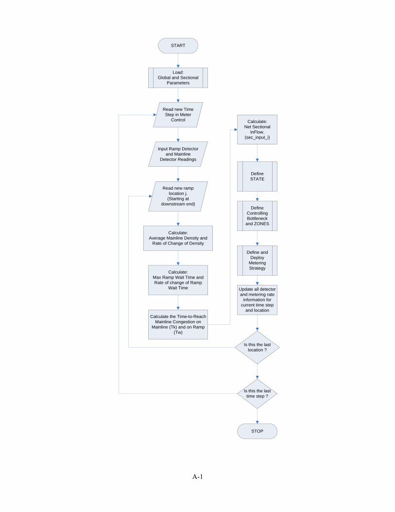
A-1

Load:Global and Sectional

Parameters

Read new Time Step in Meter

Control

Input Ramp Detector and Mainline

Detector Readings

Read new ramp location j.

(Starting at downstream end)

Calculate:Average Mainline Density and

Rate of Change of Density

Calculate:Max Ramp Wait Time and Rate of change of Ramp

Wait Time

Calculate the Time-to-Reach Mainline Congestion on

Mainline (Tk) and on Ramp (Tw)

Calculate:Net Sectional

InFlow. (sec_input_i)

Define STATE

Define Controlling Bottleneck

and ZONES

Define and Deploy

Metering Strategy

Update all detector and metering rate

information for current time step

and location

Is this the last location ?

Is this the last time step ?

STOP

START

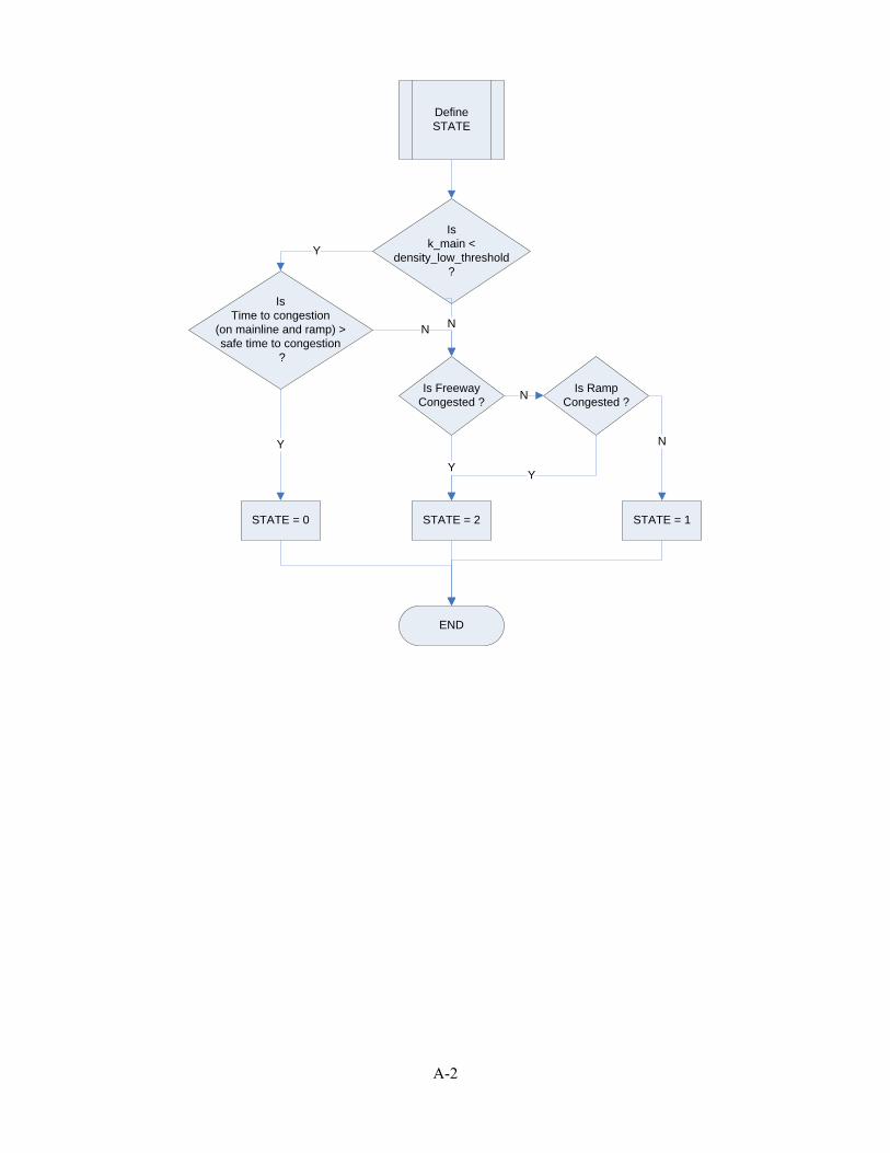
A-2

Define STATE

Is k_main <

density_low_threshold?

IsTime to congestion

(on mainline and ramp) > safe time to congestion

?

Is Freeway Congested ?

Is Ramp Congested ?

Y

NN

N

STATE = 2STATE = 0 STATE = 1

Y Y

Y N

END

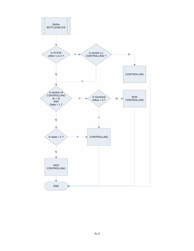
A-3

Define BOTTLENECKS

Is STATE either 1 or 2 ?

Is section j-1 CONTROLLING ?

Is section j-k CONTROLLING

(k < 3)AND

State = 1 ?

Y

N

Y

N

CONTROLLING

Is Sectional Inflow > 0 ?

NON CONTROLLINGY

NY

N

Is State = 2 ?

NON CONTROLLING

CONTROLLING

N

Y

END

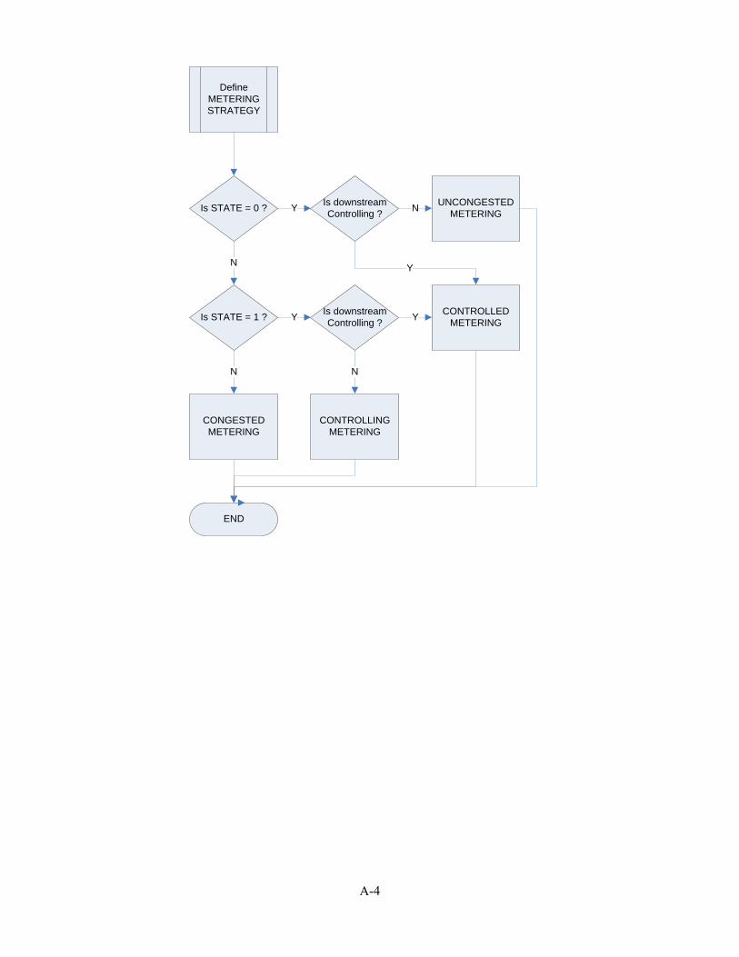
A-4

DefineMETERINGSTRATEGY

Is STATE = 0 ?

Is STATE = 1 ?

Is downstream Controlling ?

Is downstream Controlling ?

UNCONGESTED METERING

CONGESTED METERING

CONTROLLING METERING

CONTROLLED METERING

END

Y

N

Y

N

Y

N

N

Y

Appendix B:

MAP OF TEST SITE (US169-NB) (Source: Mn/DOT’s All Detector Report)

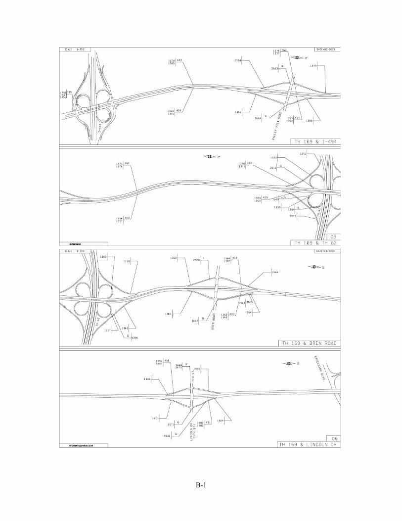
B-1

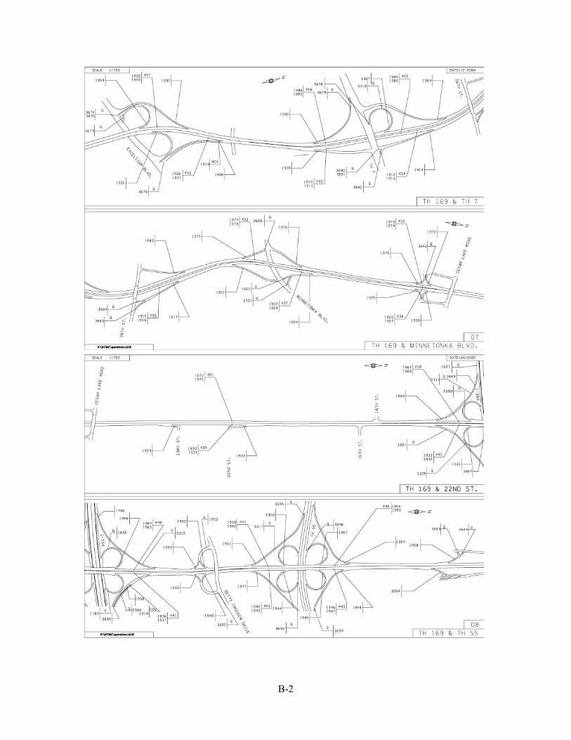
B-2

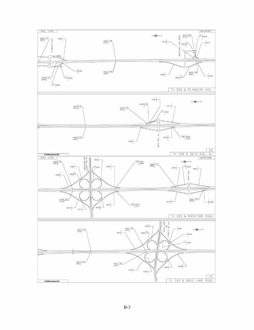
B-3