Embed Size (px)
Citation preview
DEVELOPMENT OF SOLUTION TECHNIQUESFOR
NONLINEAR STRUCTURAL ANALYSIS
FINAL REPORT
Contract NAS8-29625
September 30, 1974
Reproduced by
NATIONAL TECHNICALINFORMATION SERVICE
US Department of CommerceSpringfield, VA. 22151
Prepared by
BOEING AEROSPACE COMPANYRESEARCH AND ENGINEERING DIVISION
SEATTLE, WASHINGTON 98124
R. G. Vos - Technical Leader
J. S. Andrews - Program Leader
Prepared For
PRIES SUBJECT TO CHANGE,NATIONAL AERONAUTICS AND SPACE ADMINISTRATION
GEORGE C. MARSHALL SPACE FLIGHT CENTERMARSHALL SPACE FLIGHT CENTER, ALABAMA 35812
(NASA-CR-120525) DEVELOPMENT OF SOLUTION N75-11371TECHNIQUES FOR NONLINEAR STRUCTURALANALYSIS Final Report (Boeing AerospaceCo., Seattle, Wash.) Unclas
CSCL 20K G3/39 02589
https://ntrs.nasa.gov/search.jsp?R=19750003299 2018-07-01T22:55:57+00:00Z
THE COMPANY
D180-18325-1
DEVELOPMENT OF SOLUTION TECHNIQUES FORNONLINEAR STRUCTURAL ANALYSIS
FINAL REPORT
Contract NAS8-29625
September 30, 1974
Prepared by
BOEING AEROSPACE COMPANYRESEARCH AND ENGINEERING DIVISION
SEATTLE, WASHINGTON 98124
R. G. Vos - Technical Leader
J. S. Andrews - Program Leader
Prepared for
NATIONAL AERONAUTICS AND SPACE ADMINISTRATIONGEORGE C. MARSHALL SPACE FLIGHT CENTER
MARSHALL SPACE FLIGHT CENTER, ALABAMA 35812
THRm BEAf" COMPANY
ABSTRACT
Nonlinear structural solution methods in the current research
literature are classified according to order of the solution
scheme, and it is shown that the analytical tools for these
methods are uniformly derivable by perturbation techniques.
A new perturbation formulation is developed for treating an
arbitrary nonlinear material, in terms of a finite-difference
generated stress-strain expansion. Nonlinear geometric effects
are included in an explicit manner by appropriate definition
of an applicable strain tensor. A new finite-element pilot
computer program PANES (Program for Analysis of Nonlinear
Equilibrium and Stability) is presented for treatment of prob-
lems involving material and geometric nonlinearities, as well
as certain forms on nonconservative loading.
ii
THE fBf"LAF COMPANY
TABLE OF'CONTENTS
SECTION PAGE
TABLE OF CONTENTS iii
1.0 INTRODUCTION 1-1
1.1 General Philosophy and Evaluation of Methods 1-1
1.2 Previous Developments and Present Work 1-3
2.0 DETERMINATION OF THE EQUILIBRIUM PATH: A GENERAL- 2-1
IZATION OF STATIC PERTURBATION TECHNIQUES
2.1 Description of Nonlinearities 2-1
2.2 Formulation of Equilibrium Equations 2-3
2.3 Solution of Equilibrium Equations 2-7
3.0 DETERMINATION OF BIFURCATION AND THE POSTBUCKLING 3-1
PATH
3.1 Description of the'Postbuckling Path 3-1
3.2 Formulation of Postbuckling Equilibrium Equations 3-2
3.3 Solution of Postbuckling Equilibrium Equations 3-10
4.0 THE PANES FINITE ELEMENT PROGRAM AND NONLINEAR 4-1
SOLUTION ROUTINES
4.1 General Program Characteristics 4-1
4.2 PANES Nonlinear Analysis Routines 4-2
4.3 Summary of PANES Input Data 4-8
4.4 Summary of PANES Output 4-15
5.0 ILLUSTRATIVE PROBLEMS 5-1
5.1 Snap-Through Truss 5-1
5.2 Simple Pressure Membrane 5-4
5.3 Toroidal Membrane 5-8
5.4 Asymmetric Buckling Model 5-13
iii
THE AdA JI0 COMPANY
SECTION PAGE
6.0 CONCLUSIONS AND RECOMMENDATIONS 6-1
7.0 REFERENCES AND BIBLIOGRAPHY 7-1-
APPENDIX A: FINITE DIFFERENCE EXPANSIONS A-1
APPENDIX B: NONCONSERVATIVE LOADING EFFECTS B-1
iv
THE AIf COMPANY
1.0 INTRODUCTION
Purpose and Scope of the Study - The present research was under-
taken to develop improved techniques for solution of structures
with material and geometric nonlinearities, including the limit
point and bifurcation behavior which occurs in buckling and
collapse problems. Because the effectiveness of such solution
techniques has been found to depend strongly on the method used
for generating the nonlinear equations, e.g., creation of the
system Jacobian matrix, improved equation generation techniques
were also emphasized. Available nonlinear analysis methods
were evaluated for their current capabilities and their pro-
jected long term potentials, and the methods judged to be most
promising formed a starting point for development of the tech-
niques presented in this report. Corresponding FORTRAN sub-
routines were developed and incorporated into the pilot computer
program PANES (acronym of the Program for Analysis of Nonlinear
Equilibrium and Stability) for checkout and evaluation. The
equation generation and solution techniques are within the
framework of the finite element structural discretization method.
1.1 General Philosophy and Evaluation of Methods
Criteria - Structural solution methods available in the current
literature were initially evaluated for this study based on
four general criteria:
1. A high degree of automation which minimizes the
burden on the user.
2. Cost effectiveness for large size problems.
3. The use of an effective incremental technique which
allows the user to follow and plot the structural
response path.
4. Achievement of accuracy by a self-correcting character-
istic, which assures that the true solution is
approached at each point where results are desired.
1-1
THE Aff"WrAFAW COMPANY
During the study it was decided that recent advancements in
structural theory made it timely to broaden the applicability
of the developed equation generation and solution techniques by
including a fifth requirement:
5. An efficient treatment of large-strain problems, and
of arbitrary nonlinear elastic or inelastic materials.
Classification of Methods - The current literature contains a
very broad variety of nonlinear solution methods, and even the
specialized requirements for nonlinear structural solutions have
not resulted in consensus on a best method or methods. On the
other hand, certain types of highly nonlinear problems are
presently receiving considerable attention (for example, sta-
bility analyses and large-strain effects with arbitrary non-
linear materials), and such problems tend to eliminate certain
methods from consideration while giving some direction to future
research and development.
Most of the nonlinear structural solution methods can be broadly
grouped into three classes:
1. Methods which use only the initial (constant) stiffness
of the structure, and rely on iteration with the calcu-
lation of residual (unbalanced) forces to achieve the
correct solution. The loading may be applied incre-
mentally or in a single step.
2. Methods which form the Jacobian (tangent stiffness)
matrix at a series of load increments, without itera-
tion; also, various combined incremental and iterative
algorithms which update the Jacobian at each step or
periodically.
3. Higher-order methods (perturbation approaches or various
numerical integration schemes) which employ higher-
order derivative relations in addition to the first-
order Jacobian coefficients.
1-2
DO 6000 2140 ORIG. 4/71
THE AFAAMOW COMPANY
In many respects, the above ordering of classes is according to
increasing sophistication and greater capability. For example,
tne class 3 methods are especially suited for analysis of com-
plicated limit point and postbuckling problems. As might be
expected, the historical development of nonlinear solution methods
has shown some tendency to progress from original class 1 tech-
niques to those of classes 2 and 3.
1.2 Previous Developments and Present Work
Historical Development - Early finite-element work in nonlinear
structural analysis began with a paper by Turner, Dill, Martin
and Melosh (1960). This work incorporated nonlinear geometric
effects within the so-called "geometric" stiffness matrix, and
various incremental and iterative solution procedures were
recognized by the authors. In the initial attempts at nonlinear
solutions which followed, there was a natural tendency to gen-
eralize existing linear capabilities. This usually led to
iterative approaches and use of the initial constant stiffness
matrix, with calculation of the nonlinearities as additional
load terms. The geometric stiffness matrix, however, formed the
basis for eigenvalue buckling analyses. A more consistent and
theoretical basis for the geometric stiffness matrix was ihvesti-
gated by Gallagher and Padlog (1963), who used a strain-energy
derivation with the same displacement functions for both the
linear and nonlinear stiffness terms. Several formulations for
nonlinear beam and plate analysis soon followed. Mallett and
Marcal (1968) presented a unifying basis for formulating large
displacement problems, by deriving the total strain energy as
a function of nodal displacements and including previously
neglected nonlinear terms. Meanwhile, developments were pro-
ceeding in the area of material nonlinearities, for example the
plasticity work of Argyris (1965) and Marcal (1968), and non-
linear elastic analysis by Oden and Kubitza (1967).
1-3
THE rAf LNW COMPANY
A consensus on solution methods did hot appear, however, and
different approaches were emphasized by different research groups.
Zienkiewicz and coworkers popularized some of the class 1 solution
methods, and Zienkiewicz et al. (1969) presented a particular
method called the "initial stress" residual-load method. This work
was followed more recently by techniques for improving the inter-
ative convergence of such methods, e.g. Nayak and Zienkiewicz
(1972). However, the paper by Zienkiewicz and Nayak (1971) pre-
sents a quite general formulation for various class 2 methods with
application to combined geometric and material large-strain non-
linearities. Considerable work in geometric and material non-
linearity has been done at Brown University, for example Marcal
(1969), and McNamara and Marcal (1971). Researchers there have
tended to favor class 2 methods without iteration, although the
use of one or two iterations in each load step has been suggested
as a way of increasing accuracy. Combined incremental and inter-
ative class 2 techniques (Newton Raphson iteration, for example)
have been employed for analysis of highly nonlinear material and
geometric nonlinearities, including some stability problems, by
Oden and Key (1970), Sandidge (1973), and Key (1974). It would
certainly appear that for such problems the class 1 methods at
least are highly unsuitable. A number of nonlinear survey and
development papers have been written at Texas A & M University,
including Haisler et al. (1971), Stricklin et al. (1972),
Stricklin et al. (1973) and Tillerson et al. (1973). These papers
provide a detailed investigation of various class 1 and 2 methods,
as well as certain class 3 methods which rely on numerical inte-
gration schemes. Although perturbation procedures are not tested
by these authors, it is suggested in one of the early papers that
perturbation techniques would be very time consuming for cases
w.ith large degrees of freedom, while a more recent paper notes
that these techniques require further evaluation before they will
be accepted by structural analysts. Many other researchers work-
ing in the areas of limit point and bifurcation stability problems,
however, have concentrated on perturbation methods, reviving the
1-4
" 00 14 ORIG. 4/'1
THE COMPANY
original theoretical developmen'ts in that area by Koiter (1945).
Haftka et al. (1970) use an extension of Koiter's perturbation
theory in a solution approach called the "modified structure
method." Morin (1970) uses perturbation techniques in developing
higher-order predictor and corrector algorithms for analysis of
geometrically nonlinear shells. Gallagher and Mau (1972) and Mau
and Gallagher (1972) establish procedures for limit point and
postbuckling analysis based on perturbation expansions and the
evaluation of determinants, which employ a combination of class
1, 2 and 3 solution techniques. A number of other perturbation
developments of a more theoretical nature are included in the
references and bibliography section of this report.
Much of the present diversity in nonlinear solution methods can
be attributed to a desire to further investigate the potentials
of all methods and to compare the results obtained from them.
However, the comparisons and evaluations which are presented
often disagree in their conclusions as to the effectiveness of a
particular method. It must be surmised that the evaluation of
nonlinear solution methods is necessarily influenced by the pre-
vious experiences and preferences of the researcher, by the degree
of sophistication in his various solution method tools, and by
the type of problems toward which his interests are directed.
Direction of Present Work - Because the present work was directed
toward obtaining techniques whose applicability included the
more highly nonlinear structures, a decision was made to elimi-
nate from consideration the constant-stiffness methods of class 1.
Although schemes have been proposed for extending these methods
to more severe nonlinearities, it must be said that the arguments
given are not convincing. In fact, when the structural system has
advanced into a highly nonlinear state, the initial constant
portion of the stiffness does not really possess any more signi-
ficance than that provided by an arbitrary positive definite
matrix; it can not be expected that a technique based on this
1-5
TH rBO/, COMPANY
matrix will be of any significant value in advancing the solution
beyond the current state. It was also decided in the present
work to reject those methods of a non self-correcting nature,
i.e., methods which do not involve an iterative calculation of
the unbalanced or "residual" forces, which gives an indication
of accuracy and allows the solution to be improved. Although
such methods are sometimes effective, they can lead to serious
errors in the computed results, especially for path dependent
problems. A third group of methods eliminated from consideration
were those which use the solution data generated at several
previous solution points. Such methods essentially extrapolate
the previous data, either by some numerical integration formula
or by a curve fitting approach. These methods require storage
of previous data and are usually not self-starting. However the
main objection to their use would seem to be that the same type
of capability is provided by perturbation methods, which more
accurately evaluate the path direction and are more generally
applicable to a wide range of highly nonlinear problem types
(e.g., those involving path discontinuities such as bifurcation
points).
With these considerations, the methods which remain for develop-
ment include methods of "incremental loading", Newton Raphson
iteration and its modifications involving only periodic updating
of the Jacobian, and higher-order methods including various orders
of predictor and corrector algorithms. In order to make the
current methods applicable to cases of large strain and arbi-
trary nonlinear materials, the equation generation process is
accomplished in the present work by a finite difference expansion
procedure. It is found that generation of the nonlinear equa-
tions by this means within a perturbation context provides a
unifying basis for definition of the nonlinear solution terms,
including as special cases the first-order Newton Raphson
and incremental loading methods, as well as almost an unlimited
variety of higher-order solution techniques. The perturbation
1-6
DO 6000 2140 ORIG. 4/71

THE Aff"WWWW CoMPANY
procedures have the advantage of a sound theoretical basis in
classical developments, and lend themselves readily to both limit
point and postbuckling problems as well as to simple nonlinear
behavior without critical points.
1-7
THE BOlrVFAf COMPANY
2.0 DETERMINATION OF THE EQUILIBRIUM PATH: A GENERALIZATION OF
STATIC PERTURBATION TECHNIQUES
In this Section the theory and techniques are developed for
following the nonlinear equilibrium path of a structure under
prescribed loading. It is assumed that the equilibrium path is
continuous and unique, although limit point behavior is allowed
(the non-uniqueness due to bifurcation of the equilibrium path is
considered in Section 3. The development follows the "static
perturbation method" which was recognized and established in
concrete form by Sewell (1965). The present work generalizes
previous structural solution techniques based on the method to
allow effective treatment of arbitrary nonlinear materials. The
resulting formulation is shown to provide a quite general and
unifying basis for solution of nonlinear structures, including
geometric and material nonlinearities as well as certain forms of
nonconservative loading. A summary of the formulation is con-
tained in the paper by Vos (1974).
2.1 Description of Nonlinearities
An important characteristic of the present method is a prelim-
inary separation of the nonlinear material and geometric effects,
which minimizes the required number of perturbation expansion
terms, and also increases numerical accuracy.
Material Effects - The nonlinear material effects are described
by expanding the stress about a known equilibrium configuration:
a. = a + DO AsE + Dl A A + ... (2-1)1 1 ij i jkj 'k
which provides the stress, a, in terms of the incremental strain,Ae. Here and throughout this work, an asterisk (*) denotesquantities evaluated at a known equilibrium state, and A denotesan incremental quantity. In (2-1) a* is the initial stress, while
2-1
THE AMAMMf COMPANY
DO* and Dl* are 2nd and 3rd'order incremental stress-strain ten-
sors, respectively. This type of expansion can be developed
numerically for a general nonlinear elastic or inelastic material,
by an efficient finite difference or Taylor series evaluation.t
Complete symmetry of the D tensors can be used to advantage if they
are derivable from a strain-enery function, or in certain other
cases such as that of associative plasticity. These considerations
are discussed by Zienkiewicz and Nayak (1971) in a development
which employs only the 2nd order (DO) tensor. In any case, the
tensors can be made symmetric in the j, k and any higher order
indices.
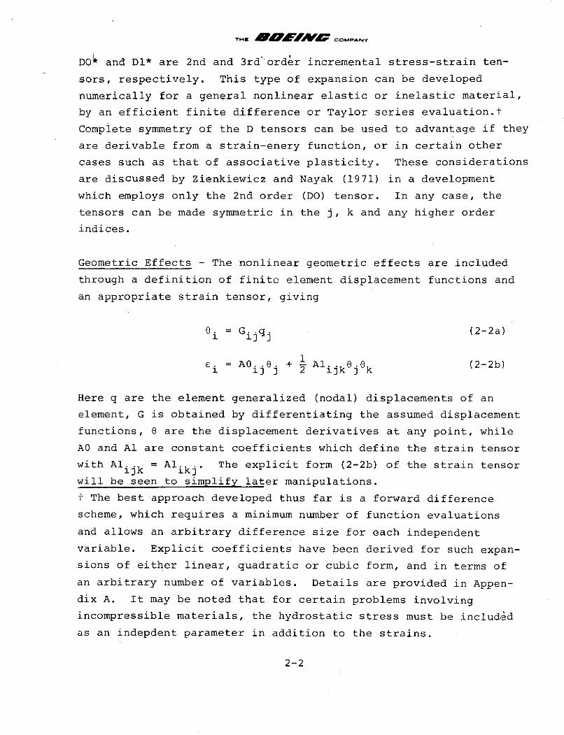
Geometric Effects - The nonlinear geometric effects are included
through a definition of finite element displacement functions and
an appropriate strain tensor, giving
6. = Gij.q. (2-2a)
6 =A0..0. + Al. k (2-2b)1 A13 j 2 1jkok
Here q are the element generalized (nodal) displacements of an
element, G is obtained by differentiating the assumed displacement
functions, 8 are the displacement derivatives at any point, while
AO and Al are constant coefficients which define the strain tensor
with Ali k = Alik j . The explicit form (2-2b) of the strain tensorijk ikj
will be seen to simplify later manipulations.
t The best approach developed thus far is a forward difference
scheme, which requires a minimum number of function evaluations
and allows an arbitrary difference size for each independent
variable. Explicit coefficients have been derived for such expan-
sions of either linear, quadratic or cubic form, and in terms of
an arbitrary number of variables. Details are provided in Appen-
dix A. It may be noted that for certain problems involving
incompressible materials, the hydrostatic stress must be included
as an indepdent parameter in addition to the strains.
2-2
THK EBOMMAOV COMPANY
Advantages of Present Approach - The present approach defines
all nonlinearities through the form of (2-1) and (2-2), rather
than through a direct expansion of the nodal displacements such
as that used in the investigation of Oden and Key (1970). The
present approach appears to offer substantial advantages,
because it allows implementation of perturbation theories into
limit point and bifurcation analysis, without involving a huge
number of terms and formidable algebraic operations. As a
practical matter, it should also be noted that a numerical
expansion based on displacements often causes severe problems
with accuracy of the expansion coefficients, due to large differ-
ences in magnitude between individual displacement limits (e.g.,
between the membrane and bending freedoms of a plate or shell),
and the selection of accurate finite difference sizes then
becomes difficult. Accuracy is more easily obtained in an
expansion of the type (2-1), because the strain limits tend to
be of the same order of magnitude.
2.2 Formulation of Equilibrium Equations
Virtual Work Statement - The principle of virtual work, which isvalid for arbitrary nonlinear materials and nonconservative sys-
tems, is employed to obtain equilibrium equations for the system
of finite elements. The formulation is developed here for aconservative system, and nonconservative effects are treated inAppendix B. The equivalence of external and internal virtual
work, relates the generalized nodal forces p and displacements
q of a particular finite element, in the element equilibrium
equation
6qip i = IV6 a a dV (2-3)
which holds along any equilibrium path in the neighborhood of
the reference equilibrium (*) configuration. Here 6E and Sqare kinematically consistent variations, and from equation (2-2)
2-3
THE 4 COMPANY
66. = G. 6q. - (2-4a)1 13 j
6r = (AOij + Al.ijkek) 68 A..66 3 B.i6qj (2-4b)
The integral in equation (2-3) is taken over the volume of the
element, and it is to be noted that a proper definition of stress
and strain is required to give the correct evaluation of internal
work. One approach for accomplishing this is a formulation of
Lagrangian strain and second Piola-Kirchoff stress integrated
over the undeformed volume, e.g. see Oden and Key (1970).
Basic Equilibrium Equation - Substituting for 66, and noting that
(2-3) must .be satisfied for arbitrary variations 6q, provides the
basic equilibrium equation for the element, as
p.i = I Baia dV = V (AOm + Alamn 6 n)a dV (2-5a)
In order to merge the element equations into the system equations,
the usual type of finite element transformation is applied. The
system forces and displacements will be denoted by the capitals
P and Q, respectively, and the system basic equilibrium equation
corresponding to (2-5a) is written as
P. = f B .a dV = (AO + Al 6n )c dV (2-5b)Sala am amn a
V V
where now it must be understood that the integral is summed over
all elements while applying the proper element-system nodal
transformations. With this understanding, the element and system
quantities will here be used interchangeably.
Derivative Relations - Equations (2-5) may now be differentiated
as many times as desired with respect to some suitable path
parameter. Toward that end, it is useful to record here the
following typical derivative relations, where an overdot (')
denotes differentiation with respect to the path parameter.
2-4
THEBA COMPANY
O= DO* + 2D1* b AE +a ab b ab b c
a = DO* E + 2Dl* Ac + 2D1* Sc + ...a ab b abc b c abc bc(2-6a)
= B .a.a aili
S=B.q. +B.q. = B.q. +Al 6a = Baii aii aii + Alamnmn
and at the reference configuration (As = 0), we have
* = DO* *a ab b
(2-6b)
* = DO* E* + 2D1* ,*E*a ab b abc b c
First Order Equilibrium Equation - Differentiating equation
(2-5b) once, and evaluating at the reference equilibrium (*) con-
figuration, gives
P" = / (B*Oa* + B*.O*) dV (2-7a)1 V al a a a
Substituting from relations (2-6b) gives
= / (G mi*Al G jq + B* DO* B* 4) dV (2-7b)1 Vmia amn n ai ab bjj
This is the first order equilibrium equation, which may be
written in the form
P= KOj Q# (2-7c)1 j J
where
KO. = (G mi*Al Gamn + B*. DO* B*) dV13 V a amn n ai ab bj
and
B*. G .A* = G (AO + Al 0*)ai mi am mi am amn n
2-5
THE BFIAAIO COMPANY
The "tangent stiffness" relation (2-7c) is equivalent to the
incremental matrix formulation of Zienkiewicz and Nayak (1971),
although the tensor form given here shows perhaps more clearly
the symmetry and differentiability properties-of the tangent
(Jacobian) matrix KO*. The first contribution to KO* is due to
the initial stresses during changing geometry, and is always
symmetric in form. The second contribution is due to the incre-
mental stress-strain relation, and its symmetry depends on
symmetry of the matrix DO*.
Second Order Equilibrium Equation - A second differentiation of
(2-5b) and evaluation at the reference configuration, gives
S= f (B*.G* + 2B*. * + B* a*)dV (2-8a)1 ai a ai a ai a
Substituting from relations (2-6b) gives
Pt = f {G *Al amnGnj + 2G .Al 8* DO* ~
1 V mia amn nj mi amn n ab b
+ B*. (DO* B*. + DO* Arsl * + 2Dbc ) dV (2-8b)al ab bqj9 ab brs r s abc b c
This is the second order equilibrium equation, which may be
written in the form
P= KO# Q* + Pl* (2-8c)1 1j J 1
where P1 is a psuedo force term given by
Pl# = / G {DO* (A* Al re** + 2A1 66*)1 mi ab am brs rs amn b n
V
+ 2D1* A* c**} dVabc am b c
2-6
THE BffCOMPANY
2.3 Solution of Equilibrium Equations
Incremental Load and Path Parameters - An increment of conserva-
tive loading is defined by
AP. =AP?, P. =A P?, etc. (2-9)1 1 1 1
using a variable load parameter A and constant nodal load
distribution Po.
Taylor series expansions are then used to approximate both the
incremental load parameter A and displacements AQ:
A =*S + *X*2 + (2-10a)A1 2
AQ = S + + ... (2-10b)1 1 2 1
In order to handle limit point situations within the present
formulation, the path parameter S is here taken as defined by
S = i KOj.AQ AQ > 0, i = + 1 (2-11)
with the requirement that KO*, evaluated at the beginning of
each load increment, be nonsingular (either positive or negative
definite). Without any loss of generality, additional require-
ments imposed at every path point, S, are that
S = = 1
S=S ... =0
Successive differentiation of (2-11) provides the relations
2SS = i KOj (Q.AQj + AQ.Q )
2 .. (2-12a)2S = i KOt (QiAQj + 2iQ + AQ Q2-12a
2-7
flfl Aflflf n A le l r i
THE AO"AAO COMPANY
(2-12a)0 = i KO# (QiAQ + 3QiQj + 3Qi Q + AQQj )
and evaluation at the reference state (S = AQi = 0), yields
2= 1 = i KO*.Q*Qi1ij 1 J
0 = i KO. (QiQ + QiQt) (2-12b)
It may be noted that relations (2-12) hold for the general case
of an unsymmetric KO* matrix.
Determination of Rate Quantities - In order to implement various
solution techniques, the equilibrium equations (2-7c) and (2-8c)
must be used to determine the load and displacement rates.
Multiplying (2-7c) by 6*, and making use of (2-9) and (2-12b),
gives
i = ~A~*P? (2-13a)1 1
Solving (2-7c) for Q* gives
KO A*P = Q* A*Q? (2-13b)j] 1 1
and substituting A*QO for Q* in (2-13a) gives
= i/(Q?P?) (2-13c)
where now i is chosen to make K* 2 positive. Multiplying (2-8c)
by Q*, and again making use of (2-9) and (2-12b), gives
QiA*Pi = KO .QtQt + QPl* -KO Q*Q* + QtPlt (2-14a)
2-8
THE Blt MOWCOMPANY
Solving (2-8c) for Q* gives
-1 *Q = KO. (A*P - Pl) A*Q? - Ql* (2-14b)1 i j j j 1 1
Substituting (2-14b) into (2-14a) with the use of (2-13c) then
provides the result
= i*2* = (PltQ? + PQl)/2 (2-14c)
after which Q* is obtained directly from (2-14b).
It is to be noted that a solution for the rates A*, A*, Q* and Q*
(and higher order rates if desired by similar calculations)
requires only a single formation and decomposition of the matrix
KO*.
Solution Procedures - Once the load and displacement rates have
been determined to a desired order, many different solution pro-
cedures can be applied in tracing the nonlinear equilibrium
path of the structure. The first order rates allow solution
by methods of incremental loading (with or without evaluation
of residual forces and corrective iterations), and Newton
Raphson iteration where the Jacobian is re-evaluated at each
iteration. Various combinations of incrementation and interation,
with periodic updating of the Jacobian are of course possible.
The second order rates allow the use of a second order predictor.
The additional cost of the 2nd order predictor is associated with
the P1 psuedo-force term, whose evaluation is performed at the
elemental level with a cost roughly proportional to that of a
single "residual force" evaluation. The cost of evaluating P1
by the form of (2-8c) is only linearly proportional to the
number of integration points within an element, so that this
technique is effective even for elements having complex geometry
and large degrees of freedom.
2-9
DC) Afoil, 4P OF~RI . d~
THE AOrJMf COMPANY
Such a predictor has been found to be very useful during the
present study, and although the PANES computer program allows
use of various predictor-corrector options, the second order
predictor almost always appears to be more efficient for cases
of substantial nonlinearity. Since the second order rates
are valid at any reference equilibrium configuration, they may
be applied in a corrector technique, at a state where the sys-
tem is in "equilibrium" under the applied loads plus a set of
unbalanced residual loads. Thus convergence could be con-
siderably accelerated if the second order relations were com-
puted and used at each iteration, although the cost per iteration
would also increase considerably. Higher order predictor-
corrector relations are obviously possible as well, and the
best type of solution capability would probably be a program
in which more or less arbitrary options are allowed for the
order of predictor and corrector, the frequency with which the
Jacobian is updated, and the number of iterations to be per-
formed per update. Although these considerations will not be
discussed in any more detail here, the PANES program is at
least a step in that direction, and makes available various
options using the first and second order rate relations.
Limit Point and Step Size Considerations - A major advantage of
a 2nd order predictor is that, with little increase in computa-
tional effort, it provides greatly increased prediction
accuracy and allows larger load steps to be taken. In addition,
it enables the traversing of limit points and provides various
techniques for automatic selection of the load step size.
In the vicinity of a limit point, the load rate relation
A = A* + A*S (2-15a)
2-10
THa COMPANY
is used. Also from (2-10a) the path value for given A is
S = { -A* + (A*2 + 2AA*)1/ 2 }/A* > 0 (2-15b)
At a limit point A = 0, so that from (2-15a) the critical path
value is
S = -*/A* (2-15c)
Using these relations the limit point can be traversed when A
is within some specified fraction of its critical value.
With regard to automatic selection of a general load step size,
the following predictor relationships are noted.
AA = As +1 S 2 (2-16a)1 2
AQi Q S + Q (2-16b)
Here the quadratic terms give an indication of the accuracy of
the linear predictor, but because of the truncation of higher
order terms there is no indication of accuracy for the quadratic
predictor. The rationale used in the PANES program implementa-
tion is therefore to select a load step size which limits the
quadratic contributions to some specified factor times the linear
contributions. Specifically, change in slope of the load
parameter during a load step is approximated by
AA = AS (2-17a)
and the ratio of slope change to average slope is
1..A/Aaverage = AS/(A + -A S) (2-17b)average 2
2-11
DO LOOO 2140 ORIG. 4/71

THE AOHJMOCOMPANY
This slope ratio is specified as a given allowable magnitude, in
order to prevent over-prediction in (2-16a) of the behavior beyond
accurate values. A similar step size restriction is employed
based on (2-16b) for displacement rates.
2-12
TH EB W COMPANY
3.0 DETERMINATION OF BIFURCATION AND THE POSTBUCKLING PATH
This section considers the identification of bifurcation points
in the load-displacement path of a structure, and the prediction
of the postbuckling path beyond these points. The formulation
follows the appraoch of Section 2 for representing geometric
nonlinearities and an arbitrary nonlinear material. The effects
of nonconservative load on bifurcation and postbuckling are
treated in Appendix B.
3.1 Description of the Postbuckling Path
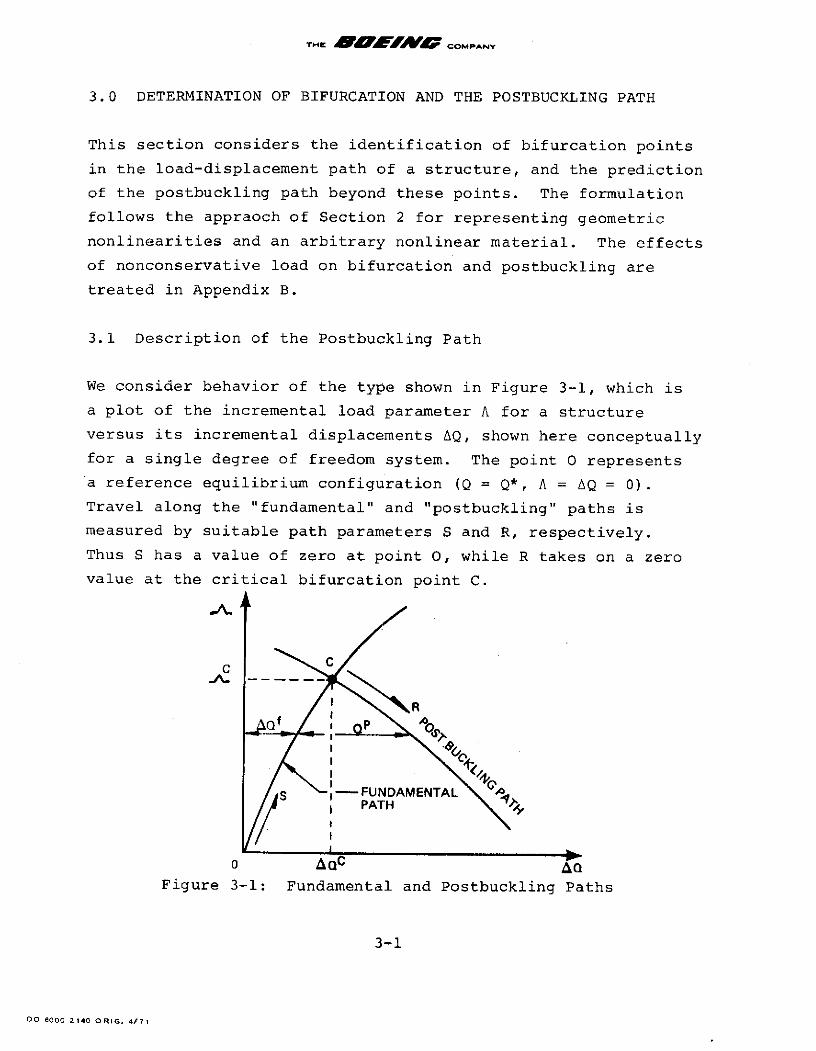
We consider behavior of the type shown in Figure 3-1, which is
a plot of the incremental load parameter A for a structure
versus its incremental displacements AQ, shown here conceptually
for a single degree of freedom system. The point 0 represents
a reference equilibrium configuration (Q = Q*, A = AQ = 0).
Travel along the "fundamental" and "postbuckling" paths is
measured by suitable path parameters S and R, respectively.
Thus S has a value of zero at point O, while R takes on a zero
value at the critical bifurcation point C.
C C-A-
/ -- FUNDAMENTALPATH
o AQC AQ
Figure 3-1: Fundamental and Postbuckling Paths
3-1
DO 6000 2140 ORIG. 4/71
THE BffWrAV COMPANY
We follow the terminology of Mau and Gallagher (1972) and use
a "sliding coordinate" system to describe the various funda-
mental and postbuckling quantities. For a given value of A,
a point on the fundamental path has associated quantities whose
values are denoted by ( ) , while additional values at the
corresponding point on the postbuckling path are denoted by ( )P
Thus total values on the postbuckling path are denoted by ( ) +
( ), and we write for the postbuckling path
Q = Q + QP
AQ = AQf + QP (3-1)
Ac = A f + P
S= o +
etc.
where the A quantities are increments from the fundamental
reference configuration.
We will refer to the ( ) and ( )P values as the "fundamental"
and "postbuckling" values, respectively, and to their sums as
the "total" values.
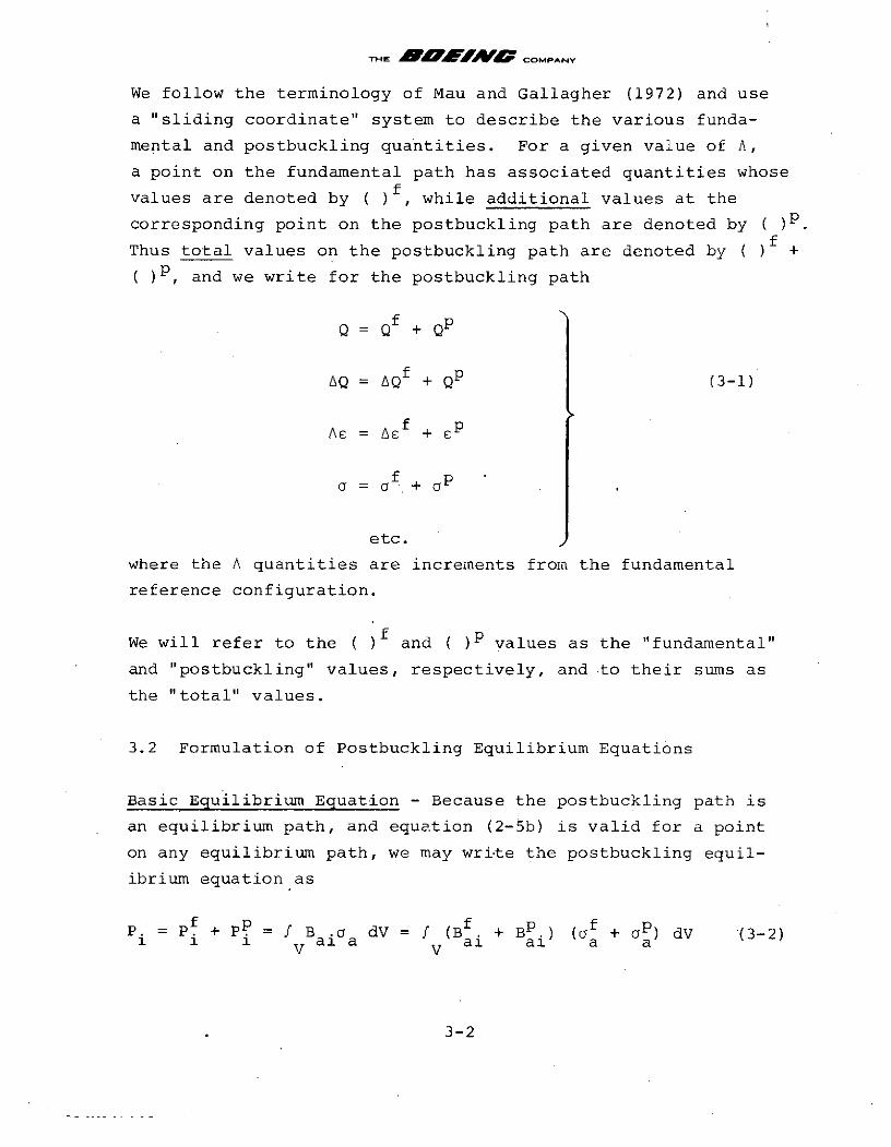
3.2 Formulation of Postbuckling Equilibrium Equations
Basic Equilibrium Equation - Because the postbuckling path is
an equilibrium path, and equation (2-5b) is valid for a point
on any equilibrium path, we may wri-te the postbuckling equil-
ibrium equation as
P. = P + P = B .a dV = f (Bf . + BP.) (a + 0P) dV (3-2)1 1 1 al a ai ail a aV V
3-2
Th E COMPANY
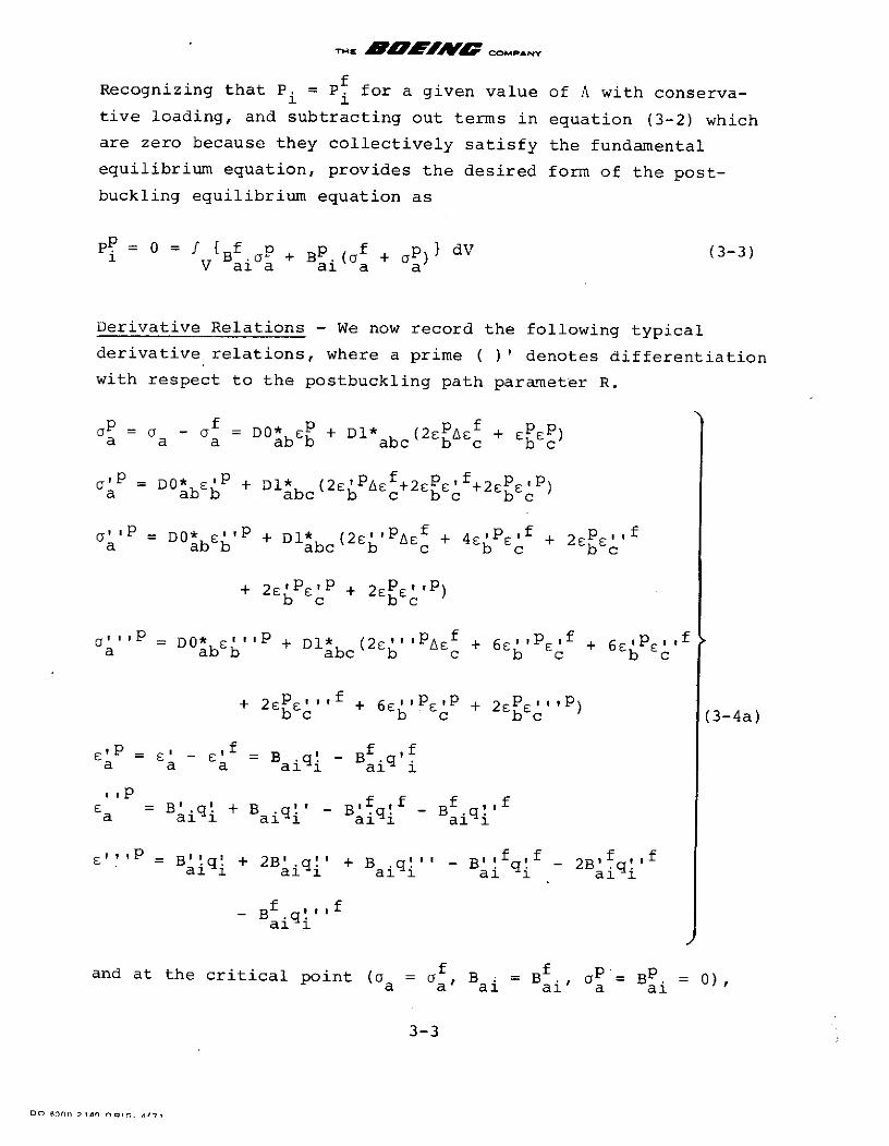
Recognizing that P. = P. for a given value of A with conserva-1 1tive loading, and subtracting out terms in equation (3-2) which
are zero because they collectively satisfy the fundamental
equilibrium equation, provides the desired form of the post-
buckling equilibrium equation as
P 0 = { f f + p} dV (3-3)V ai a al a a
Derivative Relations - We now record the following typical
derivative relations, where a prime ( )' denotes differentiation
with respect to the postbuckling path parameter R.
p = - = DO* E + Dl* (2EPAE +P 6)a a a ab b abc b c bc
a p = DO* E + Dl* (2~A fA+2p: f +2EP: P)a ab abc c bc b c
S= DO* 'p + Dl* (2' p AE f + 4 p ' f + 2: Ea abb abc b c b c bc
+ 2'P'P + 2cPeIP)b c bc
a' -= DO* ciP + D1* (2''P'As f + 6EIpcf + 6esPsfa abb abc b c c b c
+ 2PE:, t f + 6 E'PeP + 2 P P) (3-4a)bc b c bc (3-4a)
EP= E - E' = B .q! - B iq.a a al i
a aI 1 al 1 al 1 a
,f ,f f fBaiqi + 2Biq' + Biq - B qai 1 ai ai 1 ai i 2Bai
- B aiq
and at the critical point (a = a , B . = B , = B. = 0),a a ai ai a ai
3-3
DO ennn ;-4n n i.r Ai-
THE BAfAAff COMPANY
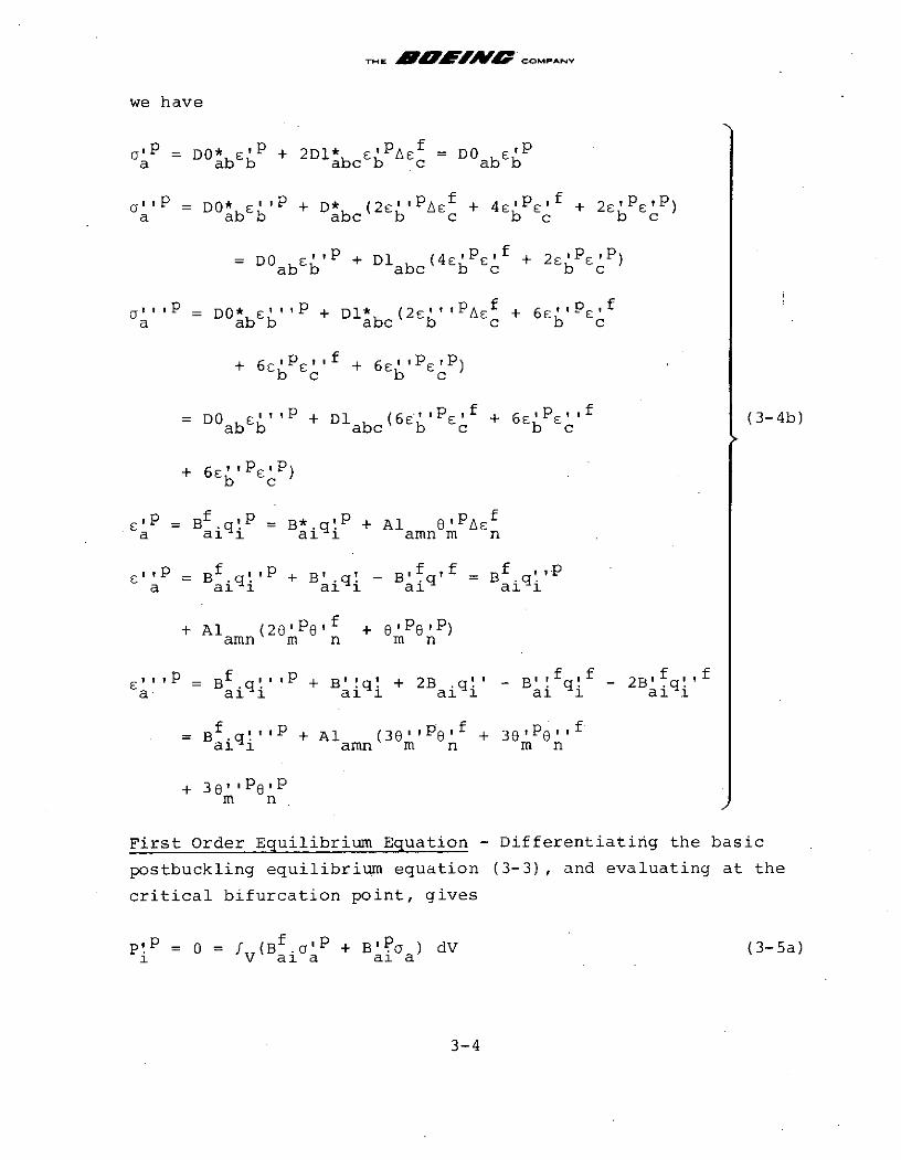
we have
P = DO* Ep + 2D1* E'PAE = DO EP
a abb abcb c ab b
Gop = DO* 'P + D* (2c'PA f + 4cP' f + 2EPEcP)a ab abc b c b c b c
= DO ,P + Dl (4Pf + 2F c'P )ab b labc b c b
" - DO* E''P + Dl* (2E'' p Af + 6E'P cfa ab b abc b c b c
+ 6 E f1 + 6E IPcIP)b c b c
=DO F l' + Dl (6f + 6P c f (3-4b)ab b abc b c b c
+ 6E 'IP P)b c
,P = B iql = B* iqP + Al a 'nP fa ai i ai I amn m n
ai = B iq + B'. q! - Bf q = B iqPS a i ai a ai
+ Al (2e'P6O f + 'IPe'P )amn m n m n
= - B .q'." + B'!q! + 2B .q!' - B' q. -2B'a aiqi ai ai ai 1 a al
f ,,p fB B 'P + Al ( 3 6 ''P 6 f + 38'Pe '
ai i amn m n m n
+ 3e' 'Pep
m n
First Order Equilibrium Equation - Differentiating the basic
postbuckling equilibrium equation (3-3), and evaluating at the
critical bifurcation point, gives
aia= 0 = (B f.'P + B'a ) dV (3-5a)V al a ai a
3-4
THE B"Orjffl COMANY
Substituting for o 'p and B'P gives
f po = f {B (DO* + 2D* A ) + GmiA l m n 'a dV (3-5b)V ai abb abc b c m an n a} dV (3-5b)
Substituting for Bai, and using the relations which express
' P and E' p in terms of q' P, gives
0 = f [(B*. + G .AlaAOf {DO* (B* '.P + Al '6 f)V a m amn ab bj j bns n s
+ 2D1* EAc f + G .Al {G .q'. p *abcb c mi amn nj 3 a
+ 8P(D 0ab f + Dl* abcfAEf) }] dV (3-5c)n ab b abc b c
This is the first order postbuckling equilibrium equation,
which may be written in the form
0 = KOj. QP + P 11 (3-5d)3 i
where again
KO . = / (Gmia*Al Gn + B*.DO* B* ) dV13 V mi a amn nj al ab bj
and
P1 = G {DO*ab (A* Al bn 'Ae + Al n PAi V mi ab am bns n s amnb n
+ Al An fe'p) + Dl* (2A* PAsf + 2A1 E'PAE: Afamn b n abc am c amn b c n
+ Al AC A ef P)}dVamn b c n
Equation (3-5d) is an eigenequation form, in terms of the
unknown critical values AO and Ae, which is suitable for
solution by power iteration.
3-5
flo n S ~l alef rr a/-r
THOE ACOMPANY
Alternatively, the eigenequation may be written in the form
0 = KO. Q'= (KO + AKO. )Q'P (3-5e)1J 3 1jj 1 j
where KO is the Jacobian at the critical point, and is given by
KOij V (GmiaAl amn Gnj + BaiDab bj) dV
with the a, DO and B quantities evaluated at the critical point.
(3-5e) may be solved directly for the eigenvector Q'P, provided
that the critical values of a, DO and B have been previously
determined (as in the method proposed by Mau and Gallagher
(1972). This equation may also be solved by expressing AKO as
a Taylor series expansion in the fundamental path parameter,
giving a form suitable for solution by one of the many "direct"
eigensolution methods.
Second Order Equilibrium Equation - A second differentiation of
the postbuckling equilibrium equation (3-3) and evaluation at
the critical point, gives
P!' = 0 = I {2B' I + B .o " + B'! p + 2B' P(u +0 ) dVi V aia al a ai a ai a a
(3-6a)
Substituting for a''p and B'"' gives
0 = [2Gmi Al 8' DO E'P + Bai DO E' p + D1 (4PIfV mi amn n ab b ai ab abc b c
+ 2E'A1)} + G .Al o''" + 2G .Al 'Pb c ml amn n a ml amnn
DOab ( f + EcP)] dV (3-6b)
3-6
THE BAf /WO COMPANY
Using the relations which express 8 ' 'P and E' 'p in terms ofq''P gives
O = [2G .Al DO + B aiDO BBbj 'P + G AV milamrr ab b a ab bj mi am
{DO (2A1 sPS'f + Al +IPP) Dl (4E PE + 26f EcP)}ab bnsn bns+n s abc b c b c
+ Al G q''P + 2G .Al nP{D0a O (E + E)}dV (3-6c)+ Gmia amnnjj mi amnn ab ]dV (3-6c)
This is the second order postbuckling equilibrium equation,
which may be written in the form
0 = KO. QI'P + 2S'P21 + P2 2 (3-6d)
where KO is again the Jacobian evaluated at the critical point,and
P21 = G {DO (A Al 'Pf + Al mr' + Al fIi mi ab am bnsn s amr r amrb r
+ 2D1 A EP } dVabc am b c
P2 2 = G .{Db (A Al 0'P' p + 2Al E'mr P)i vmi am bns n s amrb r
+ 2D1 A amPE'p } dVabc am b c
The term S' in equation (3-6d) is the derivative of the funda-mental path parameter with respect to the postbuckling pathparameter, and occurs because of the substitutions
of = 6fS,n n
,f efEf = eS'a a
(3-6d) may be solved for the postbuckling displacement secondderivatives Q'IP, and for the path derivative S'.
3-7
DO 6000 2140 ORIG. 4/71
THE A COMPANY
Third Order Equilibrium Equation - A third differentiation of
equation (3-3) and evaluation at the critical point, gives
pV'P = 0 = / {B' a + 3B' ' f ' + 3B' '" + .' 'I V ai a ai a ai a ai a
+ B'!'P( f+Gp) + 3BI!P( if+'P) + 3B'P(' f+ ' p )
al a a ai a a ai a
+ BP ( f +a 'p ) } dV .(3-7a)ai a a
Substituting for a ' and B' 'p gives
0 = 3Gmi Alamn '' DOab + 3G . Al 8' {DO l p
mi amn n ab b
+ Dlab c ( 4 P P + 2 6'PscP)}
+ B .DO l''p + Dl ( 6 i'Pscf + 6c ' f + 6C6PEP)}al abb abc b c b c b c
+ G .Al 8 ' Pml amn n a
+ 3G .miAl amn 0'P DOab (ELf + s'P) + 3Gmi .Al amn' PDO (c' +
+ Dl (2Cf el + 4C' f + 2 P P)}] dv (3-7b)
Using the relations which express 0 'p and C' ' p in terms of
q" ' gives
V m amn n ab b m amn nb abc c
+ )} B aiDO ab bj''P + G .A {DO (3A1 ''P f
b c a mam ab bnsn s
+ 3A1 bs'P 'f + 3 6''P0 P) + Dl (6Ei'Ps f + 6P''fbnsen s m n abc b c b c
+ 6"E''E')} + G . Al G q'.'P +3G .Al ''P DO(C f + COP)b c mi a amnnj J mi lamn n b
3-8
THE BOgJAf COMPANY
+ 3G Al 'P {DO (Ei'f + Es'P) + D ( 2 e f + 4 Emi am n abb b abc b c b c
+ 2E'P'P )}IdV (3-7c)
This is the third order postbuckling equilibrium equation, which
may be written in the form
0 KO. Q'." + 3S''P21 + 3P3. (3-7d)i] 3 i
where
2 p .P3 = fGmi [DO S'2 (A Alb p f + Al1 V mi ab am bnsn s amrb r
+ Al 0' P ) + S'(A Al 6bns f + Al f P + Al p6f)amr br am bns ns amr b r amrEb r
+ (A 'Al' e p OI + Al 1p" + Al E 'P P)am bns n s amr b r amr b r
+ 2D1 {S' 2 (A E + + Al E + 2A L f- )abc am b c amr b c r amr b c r
+ S'(A fec' p + Al E'P c ' + 2A1 EPrPP )am bc amrb c r amrbc r
+ (A c Pc' + Al 'p e 'P )}dVamb c AlmrEb Pc r
The term S'' occurs in (3-7d) after making the substitutions
e'f = 6 fs'n n
el = 6fS + 6S',2n n n
If *fEf = S'a a
Sf f ..f 2E' = S"' + S'
a a a
3-9
DO oo8000 2140 ORIG. 4/71
THE AO COMPANY
Equation (3-7d) may be solved for the postbuckling displacement
second derivatives .Q" 'p , and for the path second derivative S''.
3.3 Solution of Postbuckling Equilibrium Equations
The postbuckling equilibrium equations (3-5d, 6d'and 7d) may be
solved sequentially to yield the displacement and load deriva-
tives necessary for construction of the postbuckling path. These
equations have been formulated here for the general case of an
unsymmetric KO Jacobian matrix, and the effects of nonconservative
loading are discussed in Appendix B. The solution of the second
and higher order equations for the unsymmetric case present some
practical difficulties, however. Therefore, in contrast to the
general solution outlined in Section 2 for the fundamental equa-
tions, the solution given here for the postbuckling equations
will be presented for the case of a symmetric KO matrix.
First Order (Bifurcation) Solution - The first order equation
(3-5d) may be solved for the eigenvector Q'P of postbuckling dis-
placements, and for the critical value of the fundamental path
parameter S. The initial step is to relate the unknown critical
displacement increments AQ to the eigenvalue S, using the previously
computed fundamental displacement derivatives:
Qf = + Q1 si 1 2 i (3-8)
In addition to the nonlinearity inherent in this relation, the
eigenequation is nonlinear for other reasons:
1. Although increments in the displacement derivatives AG6
and displacementsAQf are linearly proportional, the strain
increments vary nonlinearly, i.e.f f 1 f f
As = A* A + Af8 fa am m 2 A1 m namn
2. There are A terms (Ae A8 , Af Af ) in the eigenequation
3-10
THE BffAAWf COMPANY
due to consideration of the nonlinear material effects
(effects of the Dl* matrix).
Because of these nonlinearities an eigensolution by direct itera-
tion may not converge. Particular difficulty may be expected
during the first few iterations, when the estimated eigenvector
contains significant proportions of higher modes for which the
Ae at some locations in the structure could be much larger than
the corresponding 8*. Also for such higher modes, the contribution
to AQ by S2 may be large and the A2 terms may be large relative
to A terms. It is therefore necessary to solve first the linear
eigen problem, obtained by dropping all nonlinear terms. When
convergence has been achieved to within a specified accuracy,
iteration is continued with inclusion of all terms until conver-
gence to the desired nonlinear eigensolution.
Higher Order Solutions - With the critical point now defined by
the critical value of S, the higher order postbuckling equations
may be solved by formation and decomposition of the critical point
Jacobian KO. To accomplish the solution, a definition of the
postbuckling path parameter R is required. We here follow the
general approach of Mau and Gallagher (1972) and take R to be one
of the postbuckling displacements, say Qm. In the PANES program,
m is taken as the index of the largest component of the eigen-
vector Q'P. We then impose the requirements at every path point,
R, that
R' = 1
R' == R''' = ... = 0 (3-9)
Although the matrix KO is singular, this constraint of the mth
degree of freedom allows the matrix to be decomposed. A somewhat
different approach than this is suggested by Haftka et al. (1970),
involving the introduction of an additional constraint equation
to make the KO matrix effectively nonsingular. That approach
3-11
nAlllo m flflICol A#"*
THE ""AJAW COMPANY
however increases the size of the matrix, and no real advantage
is seen. The present approach retains the sparsity of KO.
At this point the eigenvector Q'P is again determined, using the
constrained KO matrix. This is done to achieve consistency in
the calculation of Q'P and the higher order derivatives determined
later, as well as for greater accuracy. In terms of the symbolic-i
inverse KO :
O = KO. QP , with Q'P = 1 (3-10a)1ij 3 m
Q'P = KO. (0) (3-10b)1 13
The second order equation is
0 = KO. Q!'P + 2S'P21 + P22 , with QIP = 0 (3-11a)ij 3 j m
Premultiplying by Q'P, and using the symmetry of KO with KO. QP
= 0, results in
0o Q'KO.. Q ' + 2S'Q!~P21 + Q!PP2 = 2S'(P21+ QP2 (3-11b)i 1J J 1 1 1 1 1 1 1 1
which then gives
S' -QP2 /2Q! P21 (3-11c)1 1 1 1
and Q'P = KO- (-2S'P2 P22) E -2S'Q21 - 2 (3-11d)1 ij 3 1 i
The third order equation is
0 = KO..Q + 3(SP2 1 + P3.), with Q''P 0 (3-12a)13 3 1 1 m
Premultiplying by Q'P as before, results in
0 = S'Q!P2} + QpP3 . (3-12b)
3-12
TH 4OfA COMPANY
which then gives
S'' = -Q!PP 3 ./Q!PP21 (3-12c)1 1 1 1
and Q'P = KO. 1(-3S''P2 1 - 3P3.) -3(S'"Q21 + 3Q3i ) (3-12d)1 1J 1 1 1 1
With the critical point derivatives of S and QP known, the post-
buckling path can be constructed. The variation of load para-
meter i with postbuckling path R, is defined by
A' =AS'
A'' = A S'' +A S' (3-13)
3-13
DO nnno ;,io n ir. ir
THE BA AWIO COMPANY
4.0 FINITE ELEMENT PROGRAM AND NONLINEAR SOLUTION ROUTINES
4.1 General Program Characteristics
The major goal of this research effort was the development of
improved nonlinear solution techniques and subroutines. It was
decided that the most effective way of accomplishing this goal
was to develop a practical nonlinear finite element program, into
which the various subroutines could be incorporated for checkout
and verification. This has been accomplished, and the resulting
finite element program has been given the acronym PANES (Program
for Analysis of Nonlinear Equilibrium and Stability). Although
PANES is a pilot program and is by no means a general structural
analyzer (it utilizes only the constant strain triangle element,
for 2-D in-plane or 3-D membrane analysis) it demonstrates all
of the basic techniques and operations necessary for nonlinear
analysis by more general types of finite elements. The program
handles geometric nonlinearities and arbitrary nonlinear elastic
materials (including very large strain cases), as well as certain
forms of nonconservative loadings, i.e. those due to follower-force
pressure loadings where the surfaces change in size and orienta-
tion. Extension of the program to cases of inelastic materials
is considered to be relatively straightforward, with the intro-
duction of appropriate stress-strain constitutive relations.
The present pilot version of PANES has three basic capabilities:
1. Analysis of nonlinear structures without critical points,
i.e. tracing of simple nonlinear equilibrium paths under
a specified general (non-proportional) loading. Various
solution techniques are available, with automatic
calculation of load step sizes.
2. Traversing of limit (maximum and minimum) type critical
points, with automatic continuation of the load-path
history.
4-1

TH. E COMPANY
3. Determination of bifurcation type critical points, and
prediction of the postbuckling behavior and direction of
travel, by means of path derivatives computed at the
bifurcation point. Automatic switching from the funda-
mental path to a postbuckling path, and continuation along
the postbuckling path, have not yet been included. Thus
the postbuckling capability should be regarded as still
in a developmental stage.
4.2 PANES Nonlinear Analysis Routines
This section describes briefly the purpose and capabilities of
the program subroutines, in the order in which they appear in the
PANES program. Some of these are basic finite element routines,
while others are specialized routines needed for generating and
solving nonlinear structural equations.
BIGS - Initializes program variables (serves as the calling sub-
routine for most of the input data reading routines). Also pro-
vides problem restart capability by reading or writing the re-
start tape.
READRS - Reads data file numbers and start or restart codes.
READO - Reads problem identification title. Also reads incre-
mental and iterative constants, such as those relating to the
predictor and corrector types, the finite difference expansions
for nonlinear materials, and the techniques for continuation of
the equilibrium path through limit points.
READ1 - Reads basic structural codes and values, and material
constants for each material.
READC - Reads user-defined special nodal coordinate systems.
4-2
DO 6000 2140 ORIG. 4171
THE BffWrff COMPANY
READM - Reads mesh data, including nodal locations and coordinate
system codes, and element data.
READK - Reads codes to determine degrees of freedom with specified
forces, displacements or constraints.
READP - Reads two load reference curves which define distribution
of the applied generalized nodal loads.
READPR - Reads a pressure load reference curve which defines the
distribution of the applied pressure loads (one intensity for
each element).
READI - Reads incremental load data, including the nodal load and
pressure load curve factors for the total load at the end of
each increment.
HEAD - Writes a heading output for each load increment step,
including load parameter value, number of iterations required and
accuracy achieved.
OUTLIM - Predicts and outputs limit point values for the load
parameter, and nodal forces and displacements.
OUTPQ - Outputs nodal forces and displacements.
OUTE - Outputs element strains.
QFILL - Uses vector of system-level nodal displacements Q to form
vector of element-level nodal displacements q for an element.
PFILL - Takes vector of element-level nodal forces p and adds
them to system-level force vector P.
4-3
THE BrAFMMf COMPANY
DFILL - Uses element nodal displacement vector q to compute
vector of displacement derivatives e within the element.
EFILL - Uses element displacement derivatives vector 8 to compute
vector of strains E within the element.
AFILL - Uses element displacement derivatives 8 to form Lagrangian
AO or Al matrix within the element.
GFILL - Uses element displacement functions to form the 6-q
transformation matrix G.
MTRAN - Matrix transformation routine, which performs operations
of the type Kij = D bBaiBbj for given D and B matrices.
ROTQ - Transforms element displacements or forces, from either
nodal to element or element to nodal coordinate system.
ROTK - Transforms element stiffness matrix from element to nodal
coordinate system.
FORCE - Computes internal nodal generalized forces corresponding
to given nodal displacements.
PFORCE - Computes applied nodal force loadings, using nodal load
reference curves and corresponding load factors.
EFORCE - Computes nodal forces due to applied pressure loadings,
using pressure reference curve and factor, and the current area
and orientation of each element (determined from geometry and
current displacements).
ERCOMP - Computes and outputs error norm for each residual force
iteration, using applied (external) forces and computed (internal)
forces.
4-4
THE COMPANY
STRAIN - Computes strains for each element using geometry and
nodal displacements.
ENERGY - Evaluates the strain energy density for an element at
given strain components. This routine will in general be a user
supplied routine based on the types of materials being used in
the structure.
EVAL - Performs the function (strain energy) evaluations at the
current strain state, and at the required adjacent "perturbed"
states necessary to establish a strain energy expansion in terms
of incremental strains. EVAL calls the STRAIN routine for
evaluation, and defines the evaluation points by using the user-
specified finite difference sizes. A first, second or third
order expansion may be specified, and the corresponding function
evaluations are returned in the form of a vector.
U2FORIM - Forms coefficients for a general second order Taylor
series expansion, using function values provided by EVAL. Used
to develop the strain-energy related tensors a. and DO.- for a1 13material at current deformation state.
U3FORM - Similar to U2FORM, but forms coefficients for a general
third order expansion. Develops the tensors oi, DO.i and Dl. k
UFILL - Calling routine which calls either U2FORM or U3FORM,
depending on desired expansion order.
CFORM - Forms the contribution to the Jacobian stiffness matrix
due to the nonconservative pressure loadings.
GENER8 - Generates the elemental Jacobian matrix using the
current geometry and the material tensors o. and DO.ij. Also
adds contributions from CFORM if loading is nonconservative.
4-5
THE BAlkWO COMPANY
USUM1 - Performs a summing operation between a second or third
order tensor function and its vector argument, to give a vector.
USUM21 - Performs a summing operation between a third order
tensor function and its two (different) vector arguments, to
give a vector.
P1COMP - Computes the nonlinear load term Pl*, required in gen-
erating the second order fundamental equilibrium equations.
RATES - Computes the first and second order fundamental load
parameter and displacement rates.
STEP - Provides automatic calculation of a fundamental path load
step size, and techniques for traversing limit points.
EIGEN1 - Computes the psuedo force term P1l, for use in the
inverse power iteration eigensolution process.
EIGEN - Eigensolution routine for inverse power iteration. Calls
EIGEN1 routine.
POST2 - Computes the second order postbuckling psuedo force terms
1 2P2 or P2
POST3 - Computes the third order postbuckling psuedo force term
P3.
PRATES - Computes the first and second order postbuckling load
and displacement rates, and third order displacement rate, at
the bifurcation point.
VDOT, VCROSS, VLENTH, VNORM - Vector subroutines for computing
dot product, cross product, length, and normalizing a vector,
respectively.
4-6
DO 6000 2140 ORICr. 4A/'
THE AfEJAWf COMPANY
MERGE - Merges elemental Jacobians into system Jacobian, with
provision for constrained degrees of freedom. Forms general
unsymmetric Jacobian matrix.
DECOMP - Decomposes unsymmetric Jacobian using Gauss wavefront
type procedure. Takes advantage of sparsity but uses total
square matrix for storage without packing or external storage
devises. (This is a small pilot version decomposition routine.)
SOLVE - Performs forward and backward substitution for unsymmetric
Jacobian matrix to provide solution vectors.
4-7

TrHE F. B COMPANY
4.3 Summary of PANES Input Data
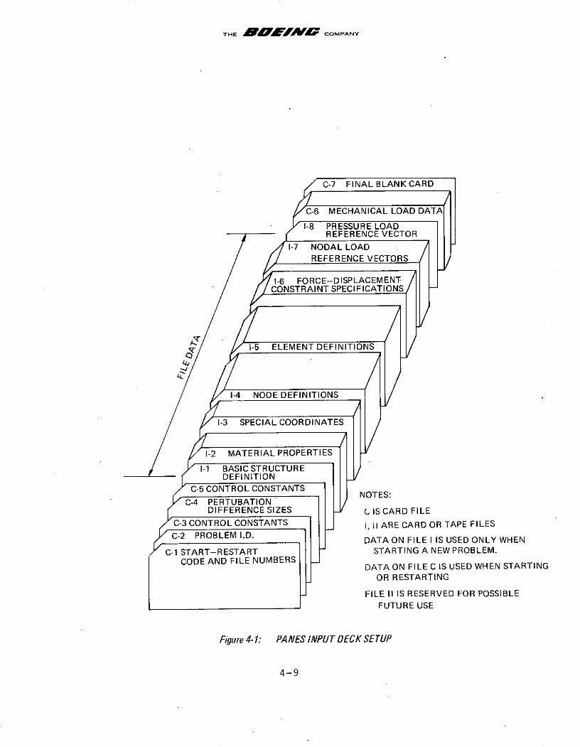
A pictorial of the PANES input deck is shown in Figure 4-1. The
input data consists of the following three general types:
Type C: Data on the usual card file. These are
data which are needed for each start or
restart.
Type I: Data on File I. These are basic structural
data for a given problem, such as material
properties and mesh data. They are the
same for all load increments and are
needed only when starting.
Type II: Data on File II. File II is not used in
the current PANES version. It is provided
for possible future use as a file of
incremental data (e.g. additional nodal
and thermal load data).
The data included on each file are described below. Formats are
consistent with FORTRAN IV conventions.
C-1. Start-restart code and data file numbers:
a. "START" if new problem, or "RESTART" if restarting.
b. If starting give unit number for file I.
c. Unit number for file II (need not be given).
d. Unit number for output file (e.g. printer).
4-8
ff nn,, an nolr- s,
THE WMPf COMPANY
C-7 FINAL BLANK CARD
C-6 MECHANICAL LOAD DATA
1-8 PRESSURE LOADREFERENCE VECTOR
1-7 NODAL LOADREFERENCE VECTORS
1-6 FORCE-DISPLACEMENTCONSTRAINT SPECIFICATIONS
1-3 SPECIAL COORDINATES
1-2 MATERIAL PROPERTIES
1-1 BASIC STRUCTUREDEFINITION
C-5 CONTROL CONSTANTS NTC-4 PERTUBATION
DIFFERENCE SIZES C IS CARD FILEC-3 CONTROL CONSTANTS _ I II ARE CARD OR TAPE FILES
DATA ON FILE I IS USED ONLY WHEN
C-1 START-RESTART STARTING A NEW PROBLEM.
DATA ON FILE C IS USED WHEN STARTINGOR RESTARTING
FILE II IS RESERVED FOR POSSIBLEFUTURE USE
Figure 4-1: PANES INPUT DECK SETUP
4-9
THE Bllf"AA COMPANY
e. If restarting give load increment number from the
end of which a restart is to be made.
f. If restarting give input restart-tape unit number.
g. If data is to be saved for future restart give out-
put restart-tape unit number.
Format (A4, 6X, 615)
C-2. Problem I.D. title.
Format (20A4).
C-3. Program control constants (any constant left blank is
assigned a default value):
a. Specified order of material incremental stress-strain
expansion to be used (2 is exact for linear material,
maximum order is 3). Default order is 3.
b. Solution predictor type. Type 1 = ist order,
Type 2 = 2nd order.
Default type = 2.
c. Maximum number of Jacobian updates per load incre-
ment step.
Default = 0.
d. Maximum number of residual force iterations per
Jacobian update.
Default = 5.
4-10
DO 6000 2140 ORIG. 4/71
THE COMPANY
e. Maximum allowable residual force error norm.
Default = 1 x 10⁻⁸.
Format (4110, F10.0)
C-4. Perturbation difference magnitudes for evaluating strain
energy.
a. Difference for computing stiffnesses.
-3Default = 1 x 10
b. Difference for computing forces.
-8Default = 1 x 10⁸.
Format (2F10.0)
C-5. Program control constants
a. Number of increment subdivisions to be performed as
load nears a limit value. Default = 3.
b. Ratio of limit load to load increment values at which
limit point is to be traversed. Default = 0.1.
c. Increment step size limitation, computed from slope
of load parameter versus path parameter curve, and
equal to change in slope divided by average slope.
Default = 0.5.
4-11
THE BWALEFMW COMPANY
d. Maximum load increment step size (used especially
in unloading), and defined as a factor times the
specified load increment.
Default = 1.0.
e. Maximum fraction of current load increment by which
load is allowed to reduce after passing a maximum
limit point.
Format (I110, 4F10.0)
I-1. Basic structure definition
a. Code for element pressure loads. Code 0 = no
pressures, Code 1 = pressures. Default code is 0.
b. Degree of freedom per node (2 or 3). No default
value.
c. Default thickness for all elements.
Format (2110, Fl0.0)
1-2. Material property definitions. For each material give
material I.D. number, and 2 material constants for use
by the strain energy evaluation routine.
Format (I110, 2F10.0)
Blank card after data for last material.
4-12
THE COMPANY
1-3. For each special Cartesian coordinate system: the
identification number (integer > 2) and counter-clockwise
angle (degrees) from basic system X-axis to special system
x-axis.
Format (I110, F10.0)
Blank card after last coordinate system.
1-4. For each node: Node number;. identification number of
coordinate system to define location; X, Y and Z (or R,
0 and Z); identification number of coordinate system to
define displacements. (Coordinate I.D. number 0 implies
the basic Cartesian system, 1 implies the basic cylindri-
cal system).
Format (215, 3F10.0, 15)
Blank card after last node.
I-5. For each element: element number, material number, thick-
ness, three node numbers (counter-clockwise order).
If thickness is left blank, default value from I-lc is
used.
Format (215, F10.0, 315)
Blank card after last element.
1-6. For each DOF with specified displacement or constraint:
If specified displacement, give node number and component
(1, 2 or 3) number;
4-13
THE "B"W* M COMPANY
If specified constraint, give node and component number,
and independent node and component to which DOF is con-
strained (independent component number is + for specified
force, - for specified displacement). User has option of
from 1 to 4 values per card.
Format (4(415))
1-7. Nodal load reference vectors.
Number of vectors (for current program version must be 2)
Format (I110)
For each nonzero component of load vector:
node number, component number (1 = X or R, 2 = Y or 8,
3 = Z), force or displacement value. User has option of
from 1 to 4 values per card.
Format (4(215, F10.0))
Blank card after last value of each vector.
1-8. Pressure Load Reference Vector. (Input only if pressure
code in data item I-1 is nonzero.
Number of vectors (for current program version must be 1)
Format (I110)
For each nonzero component of pressure load vector:
element number, pressure intensity. User has option
of from 1 to 4 values per card.
Format (4(110, F10.0))
Blank card after last value of vector.
4-14
THE B"MAZMW COMPANY
C-6. Incremental load data
Number of load increments
Format (I110)
For each load increment: solution predictor type (if
left blank, value from C-3b is used), the cumulative
factors to be applied to the nodal load reference
vectors, pressure value for all elements. Pressure is-
applied in element positive z-coordinate direction.
Format (I110, 3F10.0)
C-7. Final blank card.
Problems may be run consecutively (first data item for
each problem follows immediately after last item of pre-
ceding problem). Final blank card indicates that all
problems have been read.
4.4 Summary of PANES Output
The description of PANES output is conveniently divided into two
parts. The first is primarily an echo check of the input data,
and the second part consists of output results for each load
increment.
4.4.1 Echo Check of Input Data
Initial Output - The first page of PANES output for a problem is
essentially an echo check of input items C-1 to C-5, I-1 and
1-2. An indication is given as to whether the problem is being
started or restarted. If it is restarted then the previous
increment number is given, from the end of which the restart is
4-15
THE AOFAl a COMPANY
progressing. Next the problem I.D. title is printed, followed
by the various control constants and finite difference magni-
tudes (DFE and DFF). The limit point related control constants
(MJUMP, JUMPR, SLOPED, FLAMAX and LAMIN) are then printed. Fin-
ally the basic structural quantities from I-1, and the material
property constants from I-2 are printed.
Special Coordinate Systems - These are the user-defined direction
(special Cartesian) systems of input data item 1-3. Quantities
printed are the system number, and counter-clockwise angle (in
degrees) from the basic X axis to the special-system x axis.
Node Definitions - The information given in input item I-4 is
printed. Values are the node number, location coordinate system
number (0 = basic Cartesian, 1 = basic cylindrical), X or R
coordinate, Y or 8 (degrees) coordinate, Z coordinate, direction
coordinate system number (0 = basic Cartesian, 1 = basic
cylindrical, >1 = number of special user defined system).
Element Definitions - The information given in input item I-5
is printed. Values are the element number, material I.D. number,
element thickness, the three element node numbers in counter-
clockwise order, and the computed element area.
Force-Displacement-Constraint Prescriptions - These are the codes
given in input data item 1-6. Quantities printed are the
dependent node and component number, and independent node and
component number. (If specified displacement, no independent
numbers are given).
Nodal Load .Reference Vectors - For each input component of the
two load vectors from input item 1-7, the node number, component
number, and load value are printed.
4-16
DO 6000 2140 ORIG. 4/71
THE BAOEA CM COMPANY
Pressure Load Reference Vector - For each input component of the
pressure load vector from input item 1-8, the element number and
pressure intensity are printed.
Incremental Load Data - Quantities related to input data -item
C-6 are printed. First is printed the number of load increments
to be run. Then for each increment is given the increment num-
ber, input or default value for the predictor type, and factors.
to be applied to the two nodal load reference vectors and the
pressure load reference vector.
4.4.2 Results for Each Load Increment
Interative Error Values - An error norm computed at the end of
each iteration is printed. The error norm is obtained by a
ratio of unbalanced (residual) forces to total forces.
Increment Heading - The load increment and load step numbers
are printed, along with the load increment and load step values
at the end of the step. Following this are the nodal load
reference vector factors, the element pressure vector factor,
the predictor type for the increment, the maximum allowable
number of Jacobian updates and the numinber performed during this
load step, the maximum allowable number of iterations per update
and the number performed since the last update, and the maximum
allowable error norm and the error norm actually achieved.
Forces and Displacements - The cumulative nodal displacements
and corresponding internal forces are output. The node number
is printed, followed by the U, V and W (or R, 0, Z) components
of force and displacement.
Strains - The cumulative element strains are output. The
element number is printed, followed by the XX, YY, and XY
strains in the element coordinate system.
4-17
THE BAfffrA COMPANY
Limit Point Output - When a limit point is traversed, the pre-
dicted value of the incremental limit load parameter is output,
followed by the predicted limit forces and displacements, and
strains.
Bifurcation Point Output - When an eigenvalue solution is per-
formed to determine a critical point, the eigenvalue computed
for each inverse power iteration is printed, along with the
location of the maximum value in the eigenvector.
Decomposition Output - Whenever the Gauss decomposition routine
is called, it prints the value (sign and base 10 logarithm) of
the Jacobian stiffness determinant.
4-18
nO An ntf ffr. l -
THE B"fJZAf COMPANY
5.0 ILLUSTRATIVE PROBLEMS
Four example problems problems are presented here in order to
illustrate various aspects of nonlinear equilibrium and stability
theory, and to demonstrate use of the developed nonlinear sub-
routines and the PANES finite element program. Section 5.1
describes a snap-through truss problem with geometric nonlin-
earity and a maximum and a minimum limit point. Section 5.2
describes a simple pressure membrane with nonconservative type
loading (changing load area), resulting in a maximum limit point.
The toroidal membrane in Section 5.3 is a fairly difficult
problem, involving nonlinear (Mooney) material with follower-
force loads and changing load areas. It results in very large
displacements and strains, and a maximum and a minimum limit
point. This problem demonstrates some unique capabilities of
the PANES program. Finally, Section 5.4 describes-a simple
bifurcation/postbuckling model, with asymmetric behavior.
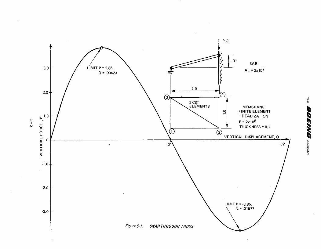
5.1 Snap-Through Truss
This is a problem similar to that used as a test case by several
researchers in nonlinear structural analysis, e.g., Haisler
et al. (1971). The system consists of a single inclined bar
(or one half of a symmetric two-member truss) as shown in
Figure 5-1. The bar has length 1.0 with axial stiffness
AE = 2x10⁷ (Hookean material), is inclined initially at a
slope of 1:100,and is subjected to a vertical end load P. The
PANES program idealization of this system used two constant
strain triangle elements, with modulas E = 2x10⁸ and thickness
= 0.1. Node 4 was constrained to have vertical displacement
equal to that at node 2, so that a system with essentially one
degree of freedom (vertical displacement Q) is obtained.
The expression for the axial strain, E, is given by
.= -. 01Q + 0.5Q 2 (5.1-1a)
5-1
PQ
S- 01 BAR
3.0- LIMIT P = 3.85, AE = 2x10 7
0 = .00423
1.02.0-
a2 CSTELEMENTS MEMBRANE
q FINITE ELEMENT
01.0 IDEALIZATIONSE = 2x10 8
LuS 0 THICKNESS = 0.1
SVERTICAL DISPLACEMENT, Q
< 0 n0.01 .02 0
wU z
-1.0
-2.0
LIMIT P = -3.85,Q =.01577
-3.0
Figure 5-1: SNAP-THROUGH TRUSS
THE iCOMPANY
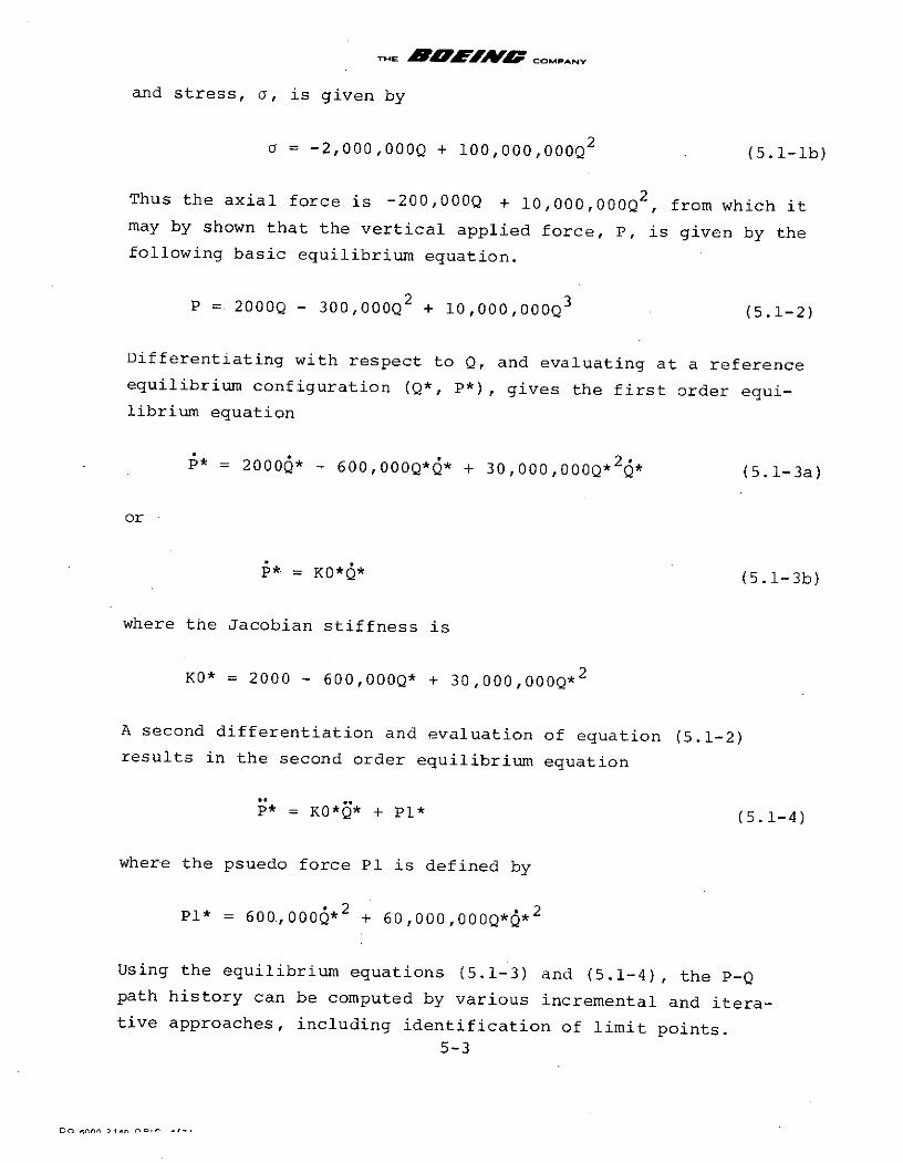
and stress, a, is given by
a = -2 ,000,000Q + 100,000,000Q (5.1-lb)
Thus the axial force is -200,000Q + 10,000,000Q 2 , from which it
may by shown that the vertical applied force, P, is given by thefollowing basic equilibrium equation.
P = 2000Q - 300,000Q 2 + 10,000,000Q 3 (5.1-2)
Differentiating with respect to Q, and evaluating at a referenceequilibrium configuration (Q*, P*), gives the first order equi-librium equation
P* = 20006* - 600,000Q** + 30,00,000Q* 26* (5.1-3a)
or
P* = KO*Q* (5.1-3b)
where the Jacobian stiffness is
KO* = 2000 - 600,000Q* + 30,000,000Q*2
A second differentiation and evaluation of equation (5.1-2)results in the second order equilibrium equation
P* = KO*Q* + Pl* (5.1-4)
where the psuedo force P1 is defined by
Pl* = 600.,000Q* 2 + 6 0,000,000Q*2
Using the equilibrium equations (5.1-3) and (5.1-4), the P-Qpath history can be computed by various incremental and itera-tive approaches, including identification of limit points.
5-3
DOgnonn i*At nr n-,
THE BAr" NM COMPANY
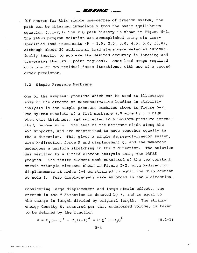
(Of course for this simple one-degree-of-freedom system, the
path can be obtained immediately from the basic equilibrium
equation (5.1-2)). The P-Q path history is shown in Figure 5-1.
The PANES program solution was accomplished using six user-
specified load increments (P = 1.0, 2.0, 3.0, 4.0, 5.0, 10.0),
although about 30 additional load steps were selected automat-
ically (mostly to achieve the desired accuracy in locating and
traversing the limit point regions). Most load steps required
only one or two residual force iterations, with usp of a second
order predictor.
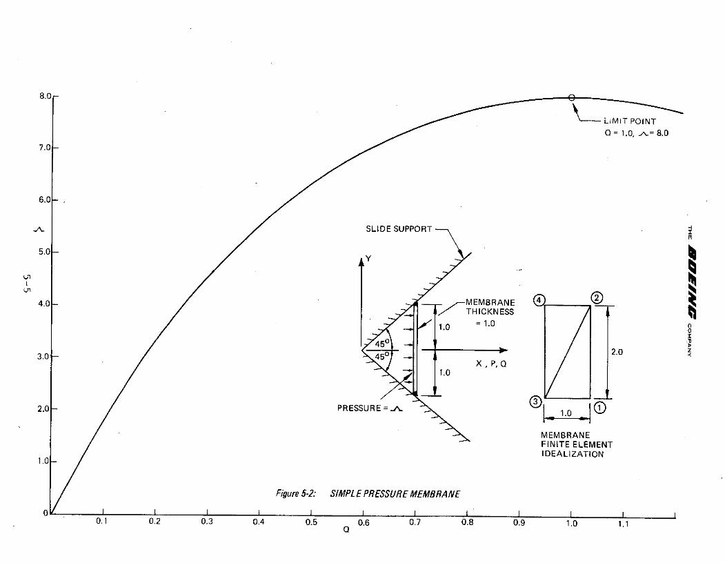
5.2 Simple Pressure Membrane
One of the simplest problems which.can be used to illustrate
some of the effects of nonconservative loading in stability
analysis is the simple pressure membrane shown in Figure 5-2.
The system consists of a flat membrane 2.0 wide by 1.0 high
with unit thickness, and subjected to a uniform pressure intens-
ity ! on one side. The ends of the membrane slide along the
450 supports, and are constrained to move together equally in
the X direction. This gives a single degree-of-freedom system,
with X-direction force P and displacement Q, and the membrane
undergoes a uniform stretching in the Y direction. The solution
was verified by a finite element analysis using the PANES
program. The finite element mesh consisted of the two constant
strain triangle elements shown in Figure 5-2, with X-direction
displacements at nodes 2-4 constrained to equal the displacement
at node 1. Zero displacements were enforced in the Z direction.
Considering large displacement and large strain effects, the
stretch in the Y direction is denoted by X, and is equal to
the change in length divided by original length. The strain-
energy density U, measured per unit undeformed volume, is taken
to be defined by the function
U = C1 (-1)2 + C2(X-l)4 = C 1Q 2 + C2 4 (5.2-1)
5-4
8.0
LIMIT POINT
O = 1.0, ,= 8.0
7.0
6.0
SLIDE SUPPORT
5.0
I
4.0- , MEMBRANE CTHICKNESS
1.0 0
450 -
3.0- 450 2.0
1.0
2.0- PRESSURE = -A- QMEMBRANEFINITE ELEMENTIDEALIZATION
1.0-
Figure 5-2: SIMPLE PRESSURE MEMBRANE
0.1 0.2 0.3 0.4 0.5 Q 0.6 0.7 0.8 0.9 1.0 1.10
THE A H1K MMAV COMPANY
Note that we could define a Lagrangian strain c, and stress-
like quantity a, by
2
U 2C Q + 4C 2 Q3aA Q 1 2
However, this is not necessary in the present problem, for
which the force can be derived directly from the strain-energy
function.
The basic equilibrium equation for the system is written using
the equivalence of external force (defined in terms of the
pressure loading ) and internal force (defined as the deriva-
tive of strain energy with respect to displacement Q):
P = 2 (l+Q) = 2(2C1 Q + 4C2 Q 3 ) (5.2-2)
Choosing specific values for the material constants Cl = 10
and C 2 = -1, the basic equilibrium equation may be written as
h (l+Q) = 20Q - 4Q3 (5.2-3)
Differentiating equation (5.2-3) provides the first order
equilibrium equation
A (l+Q) + Q = 20Q - 12Q 2 Q (5.2-4a)
or at an equilibrium configuration (k*, Q*) we can write
* = ((20 - 12Q* 2 - &*)/(l+Q*)) Q* (5.2-4b)
5-6
DO R6000 2140 ORIC. 4/1
THE "AffACOMPANY
From this equation it can be seen that the value of a Jacobianstiffness KO*, relating k * with Q*, is
KO* = (20 - 12Q* 2 - A *)/(l+Q*) (5.2-4c)
(For simplicity we have here defined the Jacobian relative toSrather than P).
Differentiating equation (5.2-3) a second time gives the secondorder equilibrium equation, as
A (l+Q) + 2iQ + Q = 20Q0 - 24Q62 - 12Q2 Q (5.2-5a)
or at an equilibrium configuration we can write
S* = KO*Q* + Pl* (5.2-5b)
where the psuedo-force P1l is given by
Pl* = (-24Q*Q*2 - 2A*Q*)/(l+Q*) (5.2-5c)
To illustrate the actual behavior of the system, we now choose Qas the path parameter, and without loss of generality specifyat every point the conditions Q = 1 and Q = 0. To aid in deter-mination of a limit type critical point, we have the conditionk* = 0 at the limit point. Using this condition, and solvingequation (5.2-4b) with the use of (5.2-3), we find a limit pointat ( * = 8.0, Q* = 1.0). The entire A-Q path history may bedetermined by various incremental and iterative predictor-corrector schemes, and is shown in Figure 5-2. The PANESprogram solution to this problem used a second-order predictorwith residual-force corrective iterations.
5-7
nfl " ' -
THE BOMAAF COPMPANY
5.3 Toroidal Membrane
The problem illustrated here is a toroidal membrane under
internal pressure, shown in Figure 5-3. This structure exhibits
a highly nonlinear type of behavior with very large displace-
ments and strains, and both a maximum and a minimum limit point.
The second-order predictor was employed in a PANES program solu-
tion, along with residual-force corrective iterations to achieve
equilibrium at each load step. Both the predictor and corrector
incorporated all changing load area and follower-force effects.
(This gave an unsymmetric KO* matrix, whose decomposition was
obtained by the Gauss wavefront procedure. It was apparent that
the unsymmetric effects became large enough that their inclusion
was necessary for convergence).
The torus was assumed to be of Mooney material with constants
C1 = 80 and C2 = 20, and was analyzed using plane-stress membraneelements. Geometry and displacement components are defined inFigure 5-3. The torus has major radius 10, minor radius 2, and
thickness .05. Cylindrical coordinates were employed to model
a wedge-shaped segment of the major circumference, of from 2 to
10 degrees arc. Constraints were employed in the radial and
vertical directions in order to equalize corresponding displace-
ments along the two sides of the wedge.
Table 5-1 summarizes computed values of key displacements for
the user-defined (input) pressure increments and the computed
limit pressures, obtained with three different meshes. (N denotes
the number of subdivisions over one half of the minor circumfer-
ence). The indicated convergence with mesh refinement is of thekind to be expected, with finer meshes giving a more flexible
structure, and resulting generally in somewhat larger displace-
ments and lower limit point values. Computer run times ranged
from 1 minute (IBM central processor time) for mesh N = 4, to7 minutes for mesh N = 12. These times should be regarded in a
5-8
no Roo ,, Osn .,,
THE AAFAB K A COMPANY
qualitative fashion only, since for example much of the timewas spent in solving the linear unsymmetric stiffness equations
and this time could be reduced by use of a production typeequation solver.
More detailed results for the fine mesh (N = 12) are shown inTable 5-2. There the data columns represent respectively the
pressure, load increment number (user-specified increment),
step number (where the PANES program automatically divided thespecified increment into a number of smaller steps), number ofresidual-force type iterations performed in order to achievethe required accuracy, and values of the radial and verticaldisplacements at key points. Figure 5-3 gives very interestingplots of two key load-displacement paths, and indicates that nodifficulties were caused by a displacement which followed anextremely irregular "doubling back" type of path, includingsharp curvature sections. The basic results for this problemare corroborated by another solution to the same problem byKey (1974), who developed a finite element program with a NewtonRaphson solution technique, and obtained results for pressurelevels up to near the first limit point.
It may be of use for comparison/test purposes to mention corre-sponding results obtained by increasing the major radius from10 to 12. Maximum and minimum limit points occurred at pressures,h, of 4.355 and 4.125, respectively, while maximum displacements(at h = 5.0) increased roughly 20 percent.
5-9
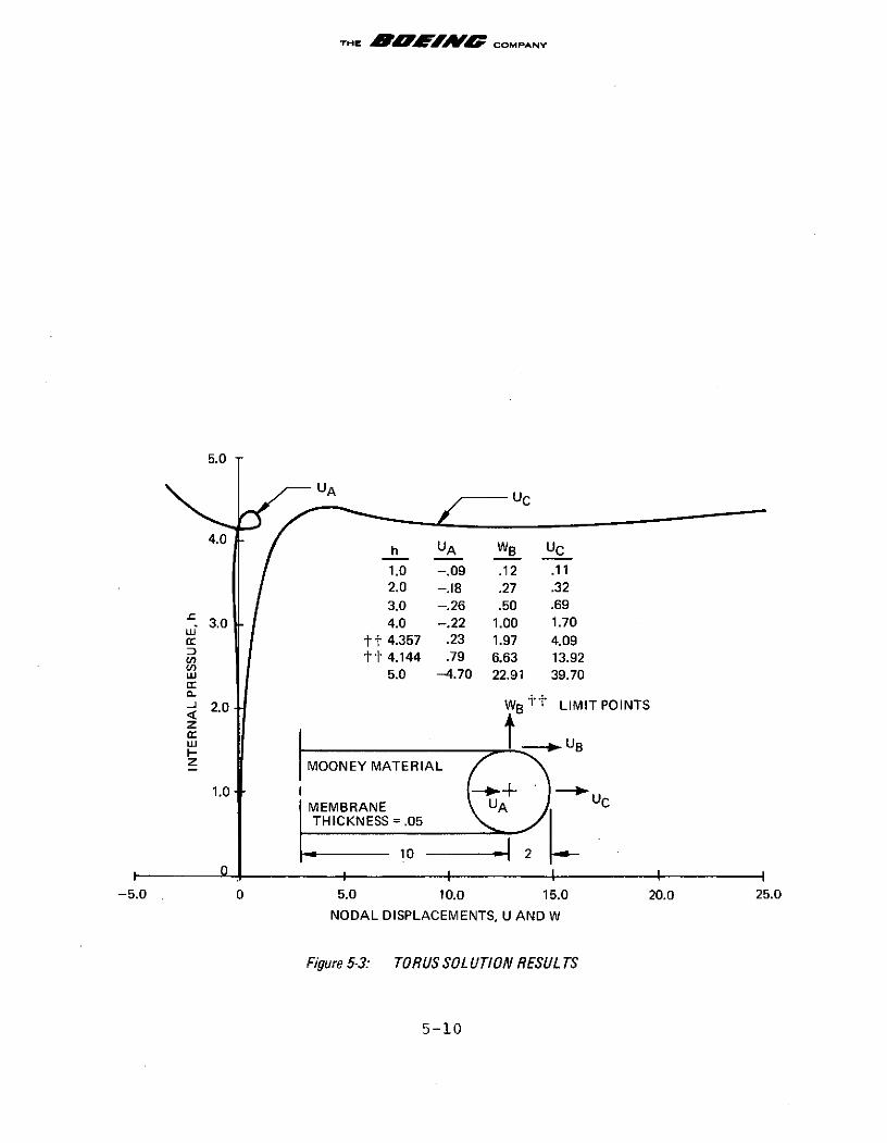
THE B""/ffJ COMPANY
5.0
U A UC
4.0 h UA WB UC
1.0 -. 09 .12 .112.0 -. 18 .27 .32
3.0 -. 26 .50 .69-- 3.0 4.0 -. 22 1.00 1.70
tt 4.357 .23 1.97 4.09c tt ±t 4.144 .79 6.63 13.92
wu 5.0 -4.70 22.91 39.70a-
-J 2.0 WB tt LIMIT POINTSz
t t UB
MOONEY MATERIAL
1.0 1 UMEMBRANE UA UCTHICKNESS = .05
10 - 2
I I I I I-5.0 0 5.0 10.0 15.0 20.0 25.0
NODAL DISPLACEMENTS, U AND W
Figure 5-3: TORUS SOL UTION RESUL TS
5-10
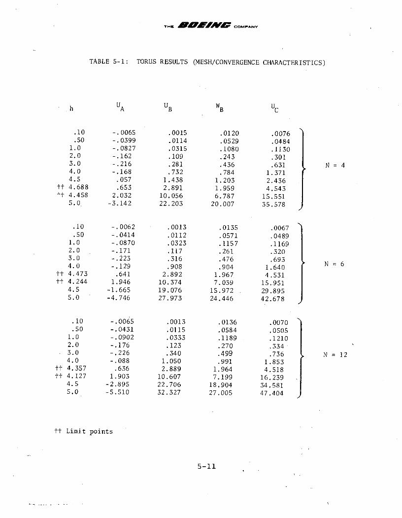
TABLE 5-1: TORUS RESULTS (MESH/CONVERGENCE CHARACTERISTICS)
h UA UB WB UC
.10 -.0065 .0015 .0120 .0076
.50 -.0399 .0114 .0529 .04841.0 -.0827 .0315 .1080 .11302.0 -.162 .109 .243 .3013.0 -.216 .281 .436 .631 N = 44.0 -.168 .732 .784 1.3714.5 .057 1.438 1.203 2.436
tt 4.688 .653 2.891 1.959 4.543tt 4.458 2.032 10.056 6.787 15.551
5.0 -3.142 22.203 20.007 35.578
.10 -.0062 .0013 .0135 .0067
.50 -.0414 .0112 .0571 .04891.0 -.0870 .0323 .1157 .11692.0 -.171 .117 .261 .3203.0 -.223 .316 .476 .6934.0 -.129 .908 .904 1.640 N = 6
tt 4.473 .641 2.892 1.967 4.531tt 4.244 1.946 10.374 7.039 15.951
4.5 -1.665 19.076 15.972 29.8955.0 -4.746 27.973 24.446 42.678
.10 -.0065 .0013 .0136 .0070
.50 -.0431 .0115 .0584 .05051.0 -.0902 .0333 .1189 .12102.0 -.176 .123 .270 .3343.0 -.226 .340 .499 .736 N = 124.0 -.088 1.050 .991 1.853
tt 4.357 .636 2.889 1.964 4.518tt 4.127 1.903 10.607 7.199 16.239
4.5 -2.895 22.706 18.904 34.5815.0 -5.510 32.327 27.005 47.404
tt Limit points
5-11
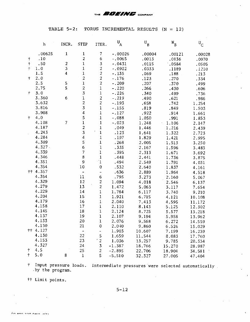
THE BAFM FM COMPANY
TABLE 5-2: TORUS INCREMENTAL RESULTS (N = 12)
h INCR. STEP ITER. UA UB WB UC
.00625 1 1 7 -.00026 .00004 .00121 .00028t .10 2 6 -.0065 .0013 .0136 .0070t .50 2 1 3 -.0431 .0115 .0584 .0505t i.0 3 i 2 -.0902 .0333 .1189 .1210
1.5 4 1 2 -.135 .069 .188 .213t 2.0 2 2 -.176 .123 .270 .334
2.5 5 1 2 -.209 .207 .370 .4992.75 5 2 1 -.220 .266 .430 .606
t 3.0 3 1 -.226 .340 .499 .7363.360 6 1 2 -.219 .490 .621 .9863.632 2 2 -.193 .658 .742 1.2543.816 3 1 -.155 .819 .849 1.5033.908 4 1 -.127 .922 .914 1.661
t 4.0 5 1 -.088 1.050 .991 1.8534.108 7 1 1 -.023 1.248 1.106 2.1474.187 2 1 .049 1.446 1.216 2.4394.243 3 1 .123 1.641 1.322 2.7234.284 4 1 .197 1.829 1.421 2.9954.309 5 1 .268 2.005 1.513 3.2504.327 6 1 .335 2.167 1.596 3.4834.339 7 1 .395 2.313 1.671 3.6924.346 8 1 .448 2.441 1.736 3.8754.351 9 1 .494 2.549 1.791 4.0314.354 10 0 .532 2.640 1.837 4.161
tt 4.357 - - .636 2.889 1.964 4.5184.354 11 6 .795 3.273 2.160 5.0674.329 12 2 1.094 4.018 2.546 6.1374.279 13 2 1.472 5.063 3.117 7.6544.229 14 1 1.784 6.117 3.740 9.2104.204 15 1 1.921 6.715 4.121 10.1084.179 16 1 2.040 7.413 4.595 11.1724.158 17 1 2.110 8.143 5.125 12.3024.145 18 1 2.124 8.725 5.577 13.2184.137 19 1 2.107 9.194 5.958 13.9624.133 20 1 2.076 9.568 6.272 14.5594.130 21 0 2.040 9.860 6.526 15.029
tt 4.127 - - 1.903 10.607 7.199 16.2394.130 22 5 1.659 11.544 8.083 17.7604.153 23 '2 1.036 13.257 9.785 20.5344.327 24 3 -1.387 18.766 15.270 28.987
t 4.5 25 2 -2.895 22.706 18.904 34.581t 5.0 8 1 5 -5.510 32.327 27.005 47.404
t Input pressure loads. Intermediate pressures were selected automatically.by the program.
tt Limit points.
5-12
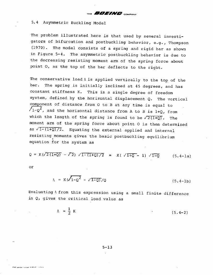
THE COMPANY
5.4 Asymmetric Buckling Model
The problem illustrated here is that used by several investi-gators of bifurcation and postbuckling behavior, e.g., Thompson(1970). The model consists of a spring and rigid bar as shownin Figure 5-4. The asymmetric postbuckling behavior is due tothe decreasing resisting moment arm of the spring force aboutpoint O, as the top of the bar deflects to the right.
The conservative load A is applied vertically to the top of thebar. The spring is initially inclined at 45 degrees, and hasconstant stiffness K. This is a single degree of freedomsystem, defined by the horizontal displacement Q. The verticalcom onent of distance from 0 to B at any time is equal to
I-Q , and the horizontal distance from A to B is 1+Q, fromwhich the length of the spring is found to be V2(It+Q). Themoment arm of the spring force about point 0 is then determinedas /1-(l+Q)/2. Equating the external applied and internalresisting moments gives the basic postbuckling equilibriumequation for the system as
Q = K(2(1+Q) - 77-2) 1-(1+Q)/2 = K( V1+Q - 1) /1-Q (5.4-la)
or
= K( / 7 - /TI---/Q (5.4-lb)
Evaluating N from this expression using a small finite differencein Q, gives the critical load value as
A 1 K (5.4-2)
5-13
flf.nn~
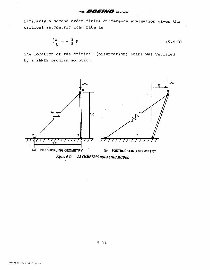
TH Bi Al-MW COMPANY
Similarly a second-order finite difference evaluation gives the
critical asymmetric load rate as
a 3- -K (5.4-3)aQ 8
The location of the critical (bifurcation) point was verified
by a PANES program solution.
IB F
1.0
(a) PREBUCKLING GEOMETRY (b) POSTBUCKLING GEOMETRY
Figure 5-4: ASYMMETRIC BUCKLING MODEL
5-14
00 A9oo 14fl ORIG. a'
THE Bf"LA COMPANY
6.0 CONCLUSIONS AND RECOMMENDATIONS
Conclusions - The present work provides improved techniques for
solution of structures with material and geometric nonlinear-
ities. FORTRAN subroutines have been developed, and incor-
porated into a new nonlinear finite-element program called
PANES (Program for Analysis of Nonlinear Equilibrium and
Stability). A new approach is developed for representing an
arbitrary nonlinear material in terms of a finite-difference
generated stress-strain expansion, and is considered to be ofmajor significance. This approach leads to formulation of
perturbation-type equilibrium equations of any desired order,
and is effective even for numerically integrated finite elements
with large degrees of freedom. The formulation should provide
a unifying basis for design of many nonlinear structural analysis
programs.
The present PANES program is a pilot version, capable of analyz-
ing problems with large strain and arbitrary nonlinear elastic
materials, and provides membrane finite elements (two or threedegrees of freedom per node) with nonconservative pressure
loading. It includes automated techniques which have been
developed for selection of load step sizes, and for locating
and traversing maximum and minimum limit-type critical points.
Subroutines are also included for location of bifurcation-type
critical points on a general nonlinear prebuckling path, and
for determining the symmetric or asymmetric postbuckling
behavior. The postbuckling capabilities have not yet been
completely automated and tested, however, and should be regarded
as being in a developmental stage.
Recommendations - The PANES program solution routines provide
a significant pilot capability for analysis of structures withhighly nonlinear material and geometric effects, and should now
6-1
THE COMPANY
be extended and evaluated for a wider class of practical
structures. Listed below are recommendations for future work.
1. The first priority should be given to improving and
verifying the PANES postbuckling subroutines. This
effort should include the generalization of program logic
to accept additional types of finite elements, and in
particular the addition of simple bar elements to the
program. These elements will simplify the study of
postbuckling results, and are desireable for initial
verification because of the somewhat complex nature of
the new nonlinear material postbuckling theory.
Automated techniques should be incorporated for branching
to the postbuckling path, similar to the existing PANES
techniques for traversing limit points.
2. The program should be extended to incorporate a number
of higher-order finite elements. Important candidate
elements are plates, shells, and isoparametric-solid
elements. Such elements will greatly extend the analysis
capabilities of the program, and also importantly demon-
strate the effectiveness of the new nonlinear solution
techniques for elements which are numerically integrated
and have large degrees of freedom.
3. PANES now handles an arbitrary nonlinear elastic material,
by use of the proper material strain-energy definition.
Formation of the stress-strain expansion relation should
be generalized to cases of inelastic material, i.e., those
materials for which a strain-energy function does not
exist. The concept of this generalization is not difficult,
but some study is required to develop an effective algor-
ithm for forming the higher-order stress-strain expansion
terms.
4. A number of largely theoretical improvements should be
studied. These include the treatment of multiple and
closely-spaced critical points (as often occur in an
optimally designed light-weight structure), and the method
6-2
DO 6000 2140 ORIG. 4/71
THE BOI ## COMPANY
of postbuckling behavior solution for cases of anunsymmetric Jacobian stiffness matrix. Incorporation ofa third-order fundamental path predictor also appearsdesireable, especially for use in prediction of bifurcation-type critical points. The nonlinear eigenvalue solution
for these points is somewhat costly, and would have tobe performed less often with the higher-order predictor.
5. The program size capability should be increased to handle
the expected range of practical nonlinear structural
problems. This involves some reorganization of the mainprogram logic, and the addition of a production-type
linear equation solver such as the Gauss-wavefront routinesused in the BOPACE elastic-plastic-creep program (Vos and
Armstrong (1973)).
6-3
T*Il BLMAMFW COMPANY
7.0 REFERENCES AND BIBLIOGRAPHY
1. Argyris, J. H., Fried, I., and Scharpf, D. W., (1968), "TheTET 20 and TEA 8 Elements for the Matrix DisplacementMethod," Journal of the Royal Aeronautical Society, Vol. 72,pp. 618-623.
2. Connor, J., and Morin, N., (1970), "Perturbation Techniquesin the Analysis of Geometrically Nonlinear Shells," HighSpeed Computing of Elastic Structures, Proceedings ofSymposium, Liege, Belgium, Vol. 2, pp. 683-705.
3. Britvec, S. J., and Chilver, A. H., (1963), "Elastic Bucklingof Rigidly-Jointed Braced Frames," Journal of the EngineeringMechanics Division, ASCE, Vol. 89, pp. 217-255.
4. Ecer, A., (1973), "Finite Element Analysis of the PostbucklingBehavior of Structures," AIAA Journal, Vol. 11, pp. 1532-1538.
5. Gallagher, R. H., and Mau, S. T., (1972), "A Method of LimitPoint Calculation in Finite Element Structural Analysis,"NASA CR-2115, National Aeronautics and Space Administration,Washington, D.C.
6. Gallagher, R. H., and Padlog, J., (1963), "Discrete ElementApproach to Structural Instability Analysis," AIAA Journal,Vol. 1, pp. 1437-1439.
7. Haftka, R. T., Mallett, R. H., and Nachbar, W., (1971),"Adaption of Koiter's Method to Finite Element Analysis ofSnap-Through Buckling Behavior," International Journal ofSolids and Structures, Vol. 7, pp. 1427-1445.
8. Haftka, R. T., Mallett, R. H., and Nachbar, W., (1970), "AKoiter-Type Method for Finite Element Analysis of NonlinearStructural Behavior, Volume I: The Modified StructureMethod," AFFDL-TR-70-130, Air Force Flight DynamicsLaboratory, Wright-Patterson Air Force Base, Ohio.
9. Haisler, W. E., Stricklin, J. A., and Stebbins, F. J.,(1971), "Development and Evaluation of Solution Proceduresfor Geometrically Nonlinear Structural Analysis by theDirect Stiffness Method," AIAA Paper No. 71-356, AIAA/ASME12th Structures, Structural Dynamics and Materials Con-ference, Anaheim, California.
10. Huseyin, K., (1973), "The Multiple-Parameter PerturbationTechnique for the Analysis of Non-Linear Systems," Inter-national Journal of Non-Linear Mechanics, Vol. 8, pp. 431-443.
7-1
DO 6000 2140 ORIG. 4/71
THE CBP oMANY
11. Hutchinson, J. W., (1973), "Post-Bifurcation Behavior in thePlastic Range," Journal of the Mechanics and Physics ofSolids, Vol. 21, pp. 163-190.
12. Hutchinson, J. W., (1973), "Imperfection Sensitivity in thePlastic Range," Journal of the Mechanics and Physics ofSolids, Vol. 21, pp. 191-204.
13. Johns, K. C. and Chilver, A. H., (1971), "Multiple PathGeneration at Coincident Branching Points, "InternationalJournal of Mechanical Sciences, Vol. 13, pp. 899-910.
14. Key, J. E., (1974), "A Note on the Numerical Solution ofCertain Problems in Finite Elasticity by the Finite ElementMethod," paper to be published in International Journal forNumerical Methods in Engineering.
15. Koiter, W. T., (1945), "Over de Stabiliteit van hetElastisch Evenwicht," Ph.D. Thesis, Technische Hogeschool,Delf, Holland. English translation (1970), "The Stabilityof Elastic Equilibrium," AFFDL-TR-70-25, Air Force FlightDynamics Laboratory, Wright-Patterson Air Force Base, Ohio.
16. Levinson, M., and Burgess, I. W., (1971), "A Comparison ofSome Simple Constitutive Relations for Slightly CompressibleRubber-Like Materials," International Journal of MechanicalSciences, Vol. 13, pp. 563-572.
17. Mallett, R. H., and Marcal, P. V., (1968), "Finite ElementAnalysis of Nonlinear Structures," Journal of the StructuralDivision, ASCE, Vol. 94, pp. 2081-2105.
18. Marcal, P.V., (1969), "Large Deflection Analysis of Elastic-Plastic Plates and Shells," Brown University TechnicalReport No. N00014-67-A-0191-0006/1.
19. Marchenko, G. A., (1966), "Solution of NonconservativeProblems in the Theory of Elastic Stability by Ritz'sMethod," Isvestiya VUZ. Aviatsionnaya Tekhnika, No. 3,pp. 62-68.
20. Mau, S. T., and Gallagher, R. H., (1972), "A Finite ElementProcedure for Nonlinear Prebuckling and Initial PostbucklingAnalysis," NASA CR-1936, National Aeronautics and SpaceAdministration, Washington, D.C.
21. McNamara, J. F., and Marcal, P. V., (1971), "IncrementalStiffness Method for Finite Element Analysis of the NonlinearDynamics Problem," Proceedings, O.N.R. InternationalSymposium on Numerical and Computer Methods in StructuralMechanics, University of Illinois.
7-2
THr Aff"AW~/ coMPANY
22. Morin, N., (1970), "Nonlinear Analysis of.Thin Shells,"Massachusetts Institute of Technology, Department of CivilEngineering, Report R70-43.
23. Murray, D. W., and Wilson, E. L., (1969), "Finite ElementLarge Deflection Analysis of Plates," Journal of theEngineering Mechanics Division, ASCE, Vol. 95, pp. 143-165.
24. Nayak, G. C., and Zienkiewicz, O. C., (1972), "Note on the'Alpha' - Constant Stiffness Method for the Analysis ofNon-Linear Problems," International Journal for NumericalMethods in Engineering, Vol. 4, pp. 579-582.
25. Nemat-Nasser, S., and Shatoff, H. D., (1973), "NumericalAnalysis of Pre- and Post-Critical Response of ElasticContinua at Finite Strains," Computers and Structures,Vol. 3, pp. 983-999.
26. Oden, J. T., and Key, J. E. (1970), "Numerical Analysis ofFinite Axisymmetric Deformations of Incompressible ElasticSolids of Revolution," International Journal of Solids andStructures, Vol. 6, pp. 497-518.
27. Osias, J. R., and Swedlow, J. L., (1974), "Finite Elasto-Plastic Deformation-I: Theory and Numerical Examples,"International Journal of Solids and Structures, Vol. 10,pp. 321-339.
28. Prasad, S. N., and Herrmann, G., (1972), "Adjoint VariationalMethods in Nonconservative Stability Problems," Inter-national Journal of Solids and Structures," Vol. 8, pp. 29-40.
29. Remmler, K. L., Cawood, D. W., Stanton, J. A., and Hill, R.,(1966), "Solutions of Systems of Nonlinear Equations,"Final Report to NASA Marshall Space Flight Center by Lock-heed Missiles and Space Company, HREC 0178-1, A-78333.
30. Sandidge, D. W., (1973), "Stability and PostbucklingBehavior of Hyperelastic Bodies at Finite Strain by theFinite Element Method," M. S. Thesis, University of Alabamain Huntsville, Huntsville, Alabama.
31. Schmit, L. A., Bogner, F. K., and Fox, R. L., (1968),"Finite Deflection Structural Analysis Using Plate andShell Discrete Elements," AIAA Journal, Vol. 6, pp. 781-791.
32. Sewell, M. J., (1965), "The Static Perturbation Techniquein Buckling Problems," Journal of the Mechanics and Physicsof Solids, Vol. 13, pp. 247-263.
7-3
DO 6000 2140 ORIG. 4/71
THE BW"AKMO COMPANY
33. Straight, J. W., (1968), "Solution to Beam Vibrations Prob-lems with Mixed Response-Excitation Input Information," AIAA/ASME 9th Structures, Structural Dynamics and Materials Con-ference, Palm Springs, California.
34. Stricklin, J. A., Haisler, W. E., and Von Riesemann, W. A.,(1972), "Computation and Solution Procedures for NonlinearAnalysis by Combined Finite Element-Finite DifferenceMethods," Computers and Structures, Vol. 2, pp. 955-974.
35. Stricklin, J. A., Haisler, W. E., and Von Riesemann, W. A.,(1973), "Evaluation of Solution Procedures for Materialand/or Geometrically Nonlinear Structural Analysis," AIAAJournal, Vol. 11, pp. 292-299.
36. Thompson, J. M. T., (1963), "Basic Principles in the GeneralTheory of Elastic Stability," Journal of the Mechanics andPhysics of Solids, Vol. 11, pp. 13-20.
37. Thompson, J. M. T., (1969), "A General Theory for theEquilibrium and Stability of Discrete Conservative Systems,"Zeitschrift fur angewandte-Mathematik und Physik," Vol. 20,pp. 797-846.
38. Thompson, J. M. T., (1970), "A New Approach to ElasticBranching Analysis," Journal of the Mechanics and Physicsof Solids, Vol. 18, pp. 29-42.
39. Thompson, J. M. T., and Hunt, G. W., (1971), "A Theory forthe Numerical Analysis of Compound Branching," Zeitschriftfir angewandte Mathematik und Physik," Vol. 22, pp. 1001-1015.
40. Tillerson, J. R., Stricklin, J. A., and Haisler, W. E.,(1973), "Numerical Methods for the Solution of NonlinearProblems in Structural Analysis," ASME Symposium on NumericalSolution of Nonlinear Structural Problems, Detroit, Michigan.
41. Turner, M. J., Dill, E. H., Martin, H. C., and Melosh, R. J.,(1960), "Large Deflections of Structures Subjected to Heatingand External Loads," Journal of the Aero/Space Sciences,Vol. 27, pp. 97-106.
42. Vos, R. G., (1970), "Finite element analysis of plate bucklingand postbuckling," Ph.D. Thesis, Rice University, Houston,Texas.
43. Vos, R. G., (1974), "Finite Element Solution of NonlinearStructures by Perturbation Technique," First InternationalConference on Numerical Methods in Nonlinear Mechanics,University of Texas at Austin, Austin, Texas.
7-4
THE 1ffAWMO COMPANY
44. Vos, R. G., and Armstrong, W. H., (1973), "BOPACE TheoreticalManual," Report on Space Shuttle Main Engine Computer Pro-gram Development, to NASA Marshall Space Flight Center byBoeing Aerospace Company, D5-17266-1.
45. Vos, R. G., and Vann, W. P., (1973), "A Finite ElementTensor Approach to Plate Buckling and Postbuckling," Inter-national Journal for Numerical Methods in Engineering, Vol.5, pp. 351-365.
46. Walker, A. C., (1969), "A Method of Solution for NonlinearSimultaneous Algebraic Equations," International Journalfor Numerical Methods in Engineering, Vol. 1, pp. 177-180.
47. Zienkiewicz, O. C., and Nayak, G. C., (1971), "A GeneralApproach to Problems of Large Deformation, and PlasticityUsing Iso-Parametric Elements," 3rd Conference on MatrixMethods in Structural Mechanics, Wright-Patterson Air ForceBase, Ohio.
48. Zienkiewicz, O. C., Valliappan, S., and King, I. P., (1969),"Elasto-Plastic Solutions of Engineering Problems 'InitialStress,' Finite Element Approach," International Journalfor Numerical Methods in Engineering, Vol. 1, pp. 75-100.
7-5
DO 6000 2140 ORIG. 4/71
THI ABMLAV COMPANY
APPENDIX A: FINITE DIFFERENCE EXPANSIONS
For the type of nonlinear solution techniques utilized in this
work, it is necessary to generate the Jacobian stiffness matrix
as well as various force-type vectors associated with residuals
and nonlinear predictor quantities. In the general case involving
nonlinear materials, these quantities cannot be effectively deter-
mined by an explicit process, and must be generated numerically.
The numerical representation may be based on a direct expansion
of the generalized forces in terms of displacements (e.g. the
method for Jacobian generation used by Oden and Key (1970)), or,
as in the approach used here, it may be based on an expansion of
stresses in terms of strains. In any case the procedure requires
the expansion of a dependent function of several independent
variables, about a known reference point.
An effective expansion procedure has been developed in the present
work by use of a Taylor series, in which the expansion coeffi-
cients (partial derivatives) are evaluated using finite differ-
ence expressions. After a study of various alternatives, it was
concluded that the most efficient scheme involves forward differ-
ences rather than central differences, because the forward differ-
ences result in simple formulas and require a minimum number of
function evaluations. In addition, if an approximate solution
path increment is known, i.e. if the approximate increments which
will occur in the independent variables are known, then a more
accurate function representation can be obtained with the forward
difference scheme by selecting the appropriate difference values.
Difference coefficients are derived here for expansions of linear,
quadratic and cubic form.
Linear Form - Coefficients for a linear expansion correspond to
those in a two-point forward difference formula. The derivation
is rather trivial, but it serves to illustrate the basic procedure.
A-1
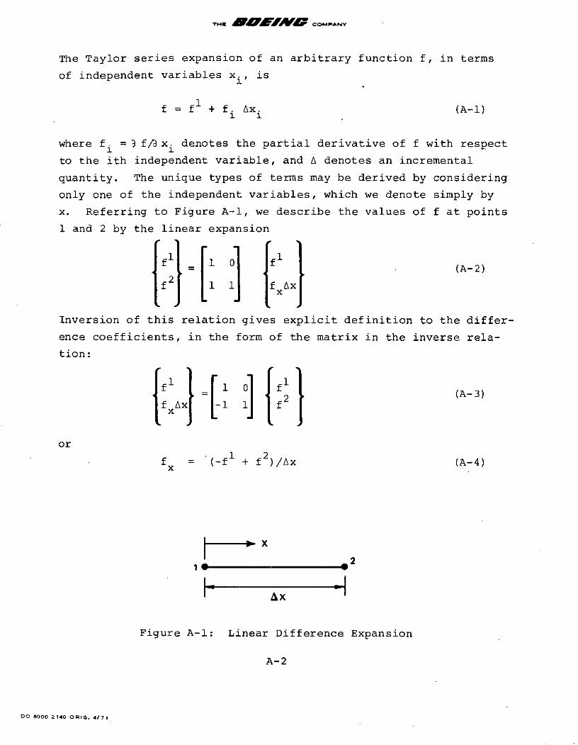
THE COMPANY
The Taylor series expansion of an arbitrary function f, in terms
of independent variables xi, is
f = f + f. Ax. (A-l)1 1
where f. = x f/ x. denotes the partial derivative of f with respect
to the ith independent variable, and A denotes an incremental
quantity. The unique types of terms may be derived by considering
only one of the independent variables, which we denote simply by
x. Referring to Figure A-1, we describe the values of f at points
1 and 2 by the linear expansionI2I= Vi (A-2)Inversion of this relation gives explicit definition to the differ-
ence coefficients, in the form of the matrix in the inverse rela-
tion:
fx = f2 (A-3)
or1 2
f = (-f + f2)/Ax (A-4)x
1 X 2I AX -I
Figure A-1: Linear Difference Expansion
A-2
DO 6000 2140 ORIG. 4/71
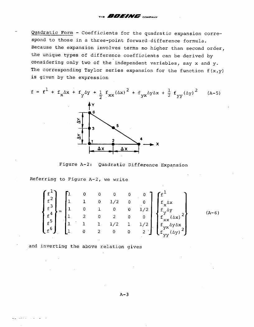
THE AfAMAOCOMPANY
Quadratic Form - Coefficients for the quadratic expansion corre-
spond to .those in a three-point forward difference formula.
Because the expansion involves terms no higher than second order,
the unique types of difference coefficients can be derived byconsidering only two of the independent variables, say x and y.
The corresponding Taylor series expansion for the function f(x,y)
is given by the expression
f 2 2f = + f Ax + f y + 1 f (Ax) + f AyAx + f (Ay) (A-5)x y 2 yxyy
tY-- 6
{ x -0*Ax
Figure A-2: Quadratic Difference Expansion
Referring to Figure A-2, we write
fl 1 0 0 0 0 0 ff2 1 1 0 1/2 0 0 f Ax3 x
f 3 1 0 1 0 0 1/2 f Ay4 Y 2 (A-6)f 1 2 0 2 0 0 fxx (Ax)
f 1 1 1 1/2 1 1/2 f AyAx6 yx 2f . 0 2 0 0 2 f (Ay)
• 1 fyy
and inverting the above relation gives
A-3
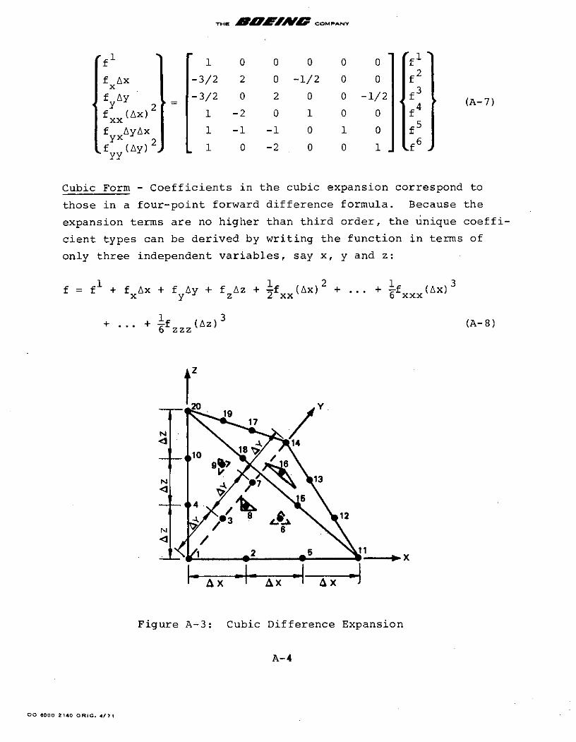
TH aOK MMW COMPANY
f 1 0 0 0 0 0 f
f Ax -3/2 2 0 -1/2 0 0 fx 3
f Ay -3/2 0 2 0 0 -1/2 fY 2 4 (A-7)
f (Ax) 1 -2 0 1 0 0 f 7xx5f AyAx 1 -1 -1 0 1 0 f
fy (Ay) 1 0 -2 0 0 1 .f6yy
Cubic Form - Coefficients in the cubic expansion correspond to
those in a four-point forward difference formula. Because the
expansion terms are no higher than third order, the unique coeffi-
cient types can be derived by writing the function in terms of
only three independent variables, say x, y and z:
f = f + fxAx + fAy + f Az + f 2 x)if (Ax)x y z +2 xx 6 xxx
+ ... + If (Az) (A-8)6 zzz
Z
19 17
s 0A 14
9 - 7 13
-b4 6
_2 X
- Ax -x Ax
Figure A-3: Cubic Difference Expansion
A-4
DO 6000 2140 ORIG. 4/71
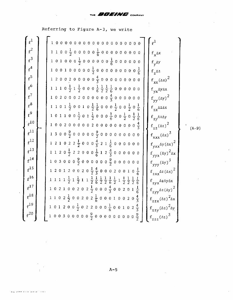
THE B"IMAKF COMPANY
Referring to Figure A-3, we write
1 1f 1 0 00 0 0 0 0 0 0 0 0 0 0 0 0 0 0 0 0 f
2 1 1f 11 00 0 0 0 0 0 0 0 0 0 0 0 0 0 fyAx2 6 x3 1 1f 1 0 1 0 0 0 0 0 0 0 0 0 0 0 0 0 0 0 f Ay2 6 y
f4 1 0 0 1 0 0 0 0 0 - 0 0 0 0 0 0 0 0 0 fAz2 6 z
f5 1 2 0 0 2 0 0 0 0 0 40 0 0 0 0 0 0 0 0 fx (Ax)2
6 1 1 1111f 1 1 0 1 0 0 0 6 2 6 0 0 0 0 0 0 f yxAyAx
43 yy8 1 11 1 1 1f 1 1 0 1 0 0 1 0 0 0 0 0 0 0 f AzAx2 26 2 2 6 zx1 1 1 1 1 1 zx
f9 1 0 1 1 0 0 0 1 0 0 0 1 0 0 1 0 1 1 f zyAZAy2 2 6 2 2 6 zy
fl0 1 0 0 2 0 0 0 0 0 2 0 0 0 0 0 0 0 0 0 f (Az) 2
3 zz (A-9)
f 1 3 0 0 0 0 0 0 0 0 0 0 0 0 0 0 0 0 f (ax)32 2 xxx
12 1 4 1 2f 1 2 1 0 2 2 0 0 0 2 1 0 0 0 0 0 0 f Ay(Ax)2 3 6 yxx
13 1 1 4 2f 11 2 0 2 2 0 0 0 0 - 1 2 - 0 0 0 0 0 0 f (Ay) Ax2 6 3 yyx
fi4 1 0 3 0 0 0 0 0 0 0 0 0 0 0 0 0 0 0 f (Ay)2 2 yyy151 4 1 (Ax)2fi5 1 2 0 1 2 0 0 2 0 1 4- 0 0 0 2 0 0 1 0 1 f Az(A)2
2z3 6 zxx16 1 1 1 1 111111 1111 f AzAyAxf 1 1 1 1 1 2 6 2 2 6 2 2 2 2 6 zyxAxS12 126226212226 zyx
f17 1 0 2 1 0 0 2 0 2 0 0 0 0 0 2 0 1 - f zyy (Ay)22 3 6 zyy
1 1 4 2f 1 1 0 2 0 0 2 0 2- 0 0 0 1 0 0 2 0- f (z) Ax2 6 3 zzx
f19 1 0 1 2 0 0 10 2 2 0 0 0 0 0 1 0 2 4 f (z)2 Ay
f20 1 0 0 3 0 0 0 0 0 90 0 0 0 0 0 0 0 0 f (Az) 3
2 2 zzz
A-5
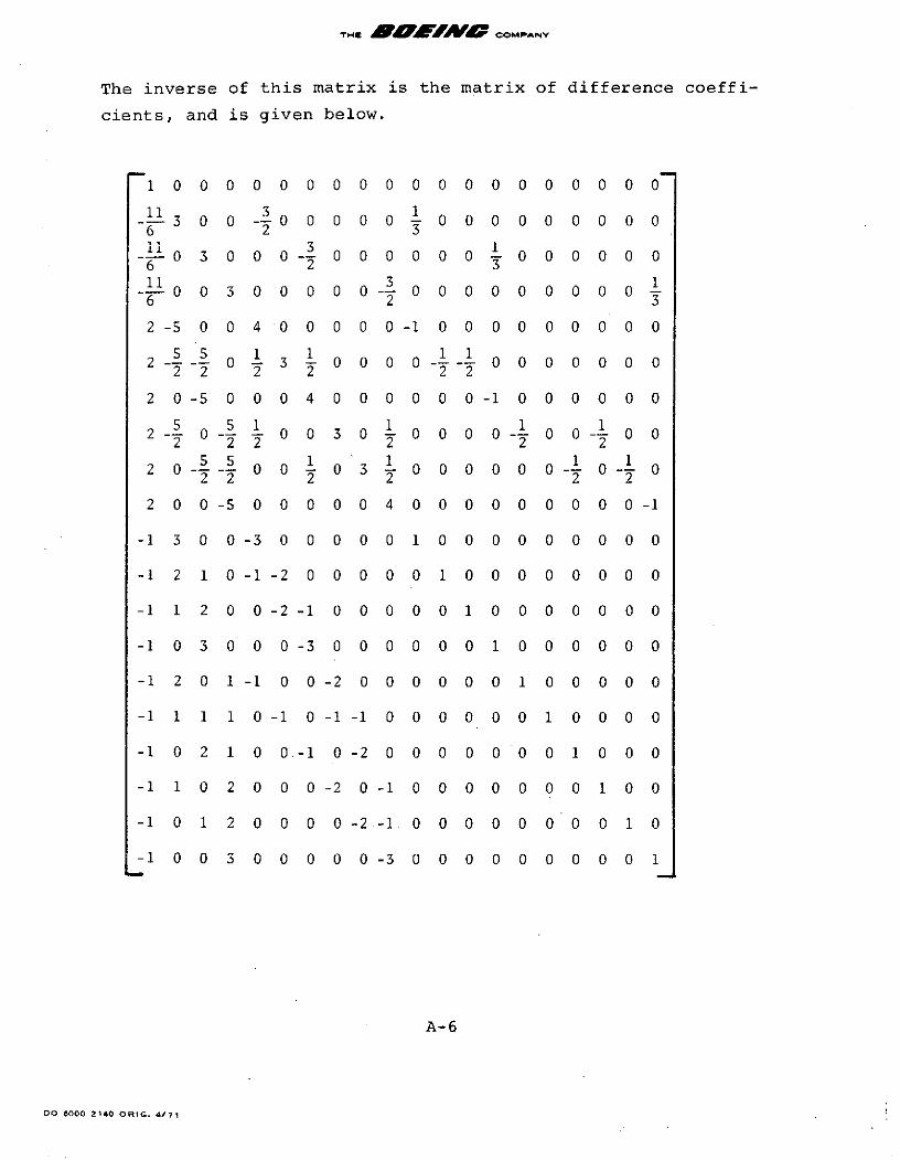
THE BOLIKOV COMPANY
The inverse of this matrix is the matrix of difference coeffi-
cients, and is given below.
1 0 0 0 0 0 0 0 0 0 0 0 0 0 00 0 0 0 0
11 3 1-10- 3 0 0 - 0 0 0 0 0 - 0 0 0 0 0 0 0 0 06 2 311ii 3 10 3 0 0 0 - 0 0 0 0 0 0 0 0 0 0 0
11 3 100300000-- 00000 0000-
6 2 3
2 -5 0 0 4 0 0 0 0 0 -1 0 0 0 0 0 0 0 0
55 1 1 112 550 i 3i 0 0 0 0 0 0 0 0 0 022 2 2 2 20
2 0 -5 0 0 0 4 0 0 0 0 0 0 -1 0 0 0 0 00
5 5 1 1 1 12 0 0-5 0 0 0 3 0 0 000 0--0 0 -- 0 0-12 22 2 2 2
55 1 1 1 12 0 0-3 00 03 0 0 0 0 0 0 0--0 --0
22 2 2 2 2
2 0 0 -5 0 0 0 0 0 4 0 0 0 0 0 0 0 0 0 -1
-1 3 0 0-3 0 0 0 0 0 1 0 0 0 0 0 0 0 0 0
-1 2 10 -1 -2 0 0 0 0 0 1 0 0 0 0 0 0 0 0
-1 1 2 0 0 -2 -1 0 0 0 0 0 1 0 0 0 0 0 0 0
-1 0 3 0 0 0 -3 0 0 0 0 0 0 1 0 0 0 0 0 0
-1 2 0 1 -1 0 0 -2 0 0 0 0 0 0 1 0 0 0 0 0
-1 1 1 1 0 -1 0 -1 -1 0 0 0 0 0 0 1 0 0 0 0
-1 0 2 1 0 0 -1 0 -2 0 0 0 0 0 0 0 1 0 0 0
-1 1 0 2 0 0 0 -2 0 -1 0 0 0 0 0 0 0 1 0 0
-1 0 1 2 0 0 0 0 -2-1 0 0 0 0 0 0 0 0 1 0
-1 0 0 3 0 0 0 0 0 -3 0 0 0 0 0 0 0 0 0 1
A-6
DO 6000 2140 ORIG. 4/71
THE MMMMP COMPANY
Organization of Terms - The number of unique terms in a symmetric
tensor of order M and dimension N, is summarized as follows.
Order Number of Terms
0 1
1 N
2 N(N+1)/2
3 N(N+1)(N+2)/6
M N(N+1)(N+2) ... (N+M-1)/M!
These relations also give the number of unique Mth order partial
derivatives involved in an Mth ' order Taylor series expansion of
N variables. For example, the coefficients of a second-order
expansion in three variables (x,y,z) are the 3(3+1)/2 = 6 second
partial derivatives (xx,yx,yy,zx,zy,zz). The total number of
terms required in the expansion is the sum of the numbers of
partial derivatives of each order, for example a second-order
expansion in three variables requires 1 + 3 + 3(3+1)/2 = 10 total
terms, and therefore a minimum of 10 function evaluations to deter-mine the coefficient (partial derivative) values.
The required coefficients for an expansion are conveniently organ-
ized into a one dimensional array, for example for a function ofthree variables the array is
1(f fl f2 f3 fll f21 f22 f31 ' f ll )
The terms are then easily retrieved from this array using the
tensor relations given above. Thus using Li, Lij, Li jk ... to
denote the location of the respective i, ij, ijk, ... derivativeterms within the array, we have for a function of N variables
L 1 L = L00 + (i-l) (i)/2 + j
L. = L + i L - L + N(N+1)/21 0 000 00L E 1 + N Lij k = L000 + (i-l)(i)(i+l)/6
+ (j-1)(j)/2 + k
A-7
THC EFMAKMO COMPANY
General Discussion - It may be observed that the forward differ-
ence scheme outlined here requires a minimum number of function
evaluations, i.e. one plus the number of partial derivatives
involved in the expansion. Along with its other advantages of
possible improved accuracy in certain types of situations, this
would seem to indicate that the forward difference formulas pre-
sented here constitute the best approach for the required function
expansions.
An interesting alternative derivation of the difference coeffi-
cient matrices is possible by a procedure used in the finite
element method. The function to be expanded may be thought of as
the quantity (say displacement) being interpolated within the
finite element. The function is then defined in terms of its
values at the nodes (i.e. the independent variable values) times
the corresponding shape functions. The required partial deriva-
tives can then be evaluated explicitly at the "origin", i.e. a
corner node at which the sides of the element form an orthogonal
coordinate system, simply by differentiating the element shape
functions. Of course the appropriate finite element shape
functions must be available, but if they are then this process
allows derivation of the difference formulas without inversion
of a matrix. These considerations were initially responsible for
the selection of the forward difference approach, and the second
and third order coefficients were evaluated in this manner, for
example the third order coefficients using the TET 20 element of
Argyris et al. (1968).
A-8
DO 6000 2140 ORIG. 4/71
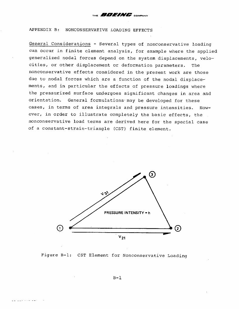
THE BlffWCOMPANY
APPENDIX B: NONCONSERVATIVE LOADING EFFECTS
General Considerations - Several types of nonconservative loading
can occur in finite element analysis, for example where the applied
generalized nodal forces depend on the system displacements, velo-
cities, or other displacement or deformation parameters. The
nonconservative effects considered in the present work are those
due to nodal forces which are a function of the nodal displace-
ments, and in particular the effects of pressure loadings where
the pressurized surface undergoes significant changes in area and
orientation. General formulations-may be developed for these
cases, in terms of area integrals and pressure intensities. How-
ever, in order to illustrate completely the basic effects, the
nonconservative load terms are derived here for the special case
of a constant-strain-triangle (CST) finite element.
PRESSURE INTENSITY - h
V2 1
Figure B-l: CST Element for Nonconservative Loading
B-1
THE N MLVAMW COMPANY
CST Element Definitions - Referring to Figure B-I, consider the
CST element with nodes 1, 2 and 3, and subjected to a normal
pressure loading of intensity h. The vectors V 21 and V3 1 connect
the nodes 1-2 and 1-3, respectively. The cross product V 2 1 x V31is then a vector with (positive) direction normal to the element
surface and with magnitude equal to twice the element area.
Coordinates in the initial configuration are defined by the com-
ponents x,y,z, and corresponding displacements by u,v,w. Then
by defining for node k, the quantities
cxk = (xk + uk) -(x1 +u)
cyk = (Yk +Vk) - (Y 1 +V 1 ) (B-la)
Czk = (zk+wk) - (z1 +w 1)
we may write the vectors V as
V 21 7 (cx 2 ,cy 2 CZ 2 ) -bV (B-b)V31 = (cx3'cy 3 ,c 3 )
while their rates are given by
21 = (u 2 ul , 2 1 ,w2 _) 1 (B-lc)V31 (u3-u1 , 3v 1 ,w3 w1 J
B.1 Fundamental Equilibrium Formulation
In this section the nonconservative loading effects are formulated
for the CST element, and used to generalize the fundamental equi-
librium equations in Section 2 to analysis of nonconservative
systems.
B-2
00 6000 2140 ORIG. 4/71
THa MAPALMg COMPANY
Basic Load Equation - For a uniform pressure loading, each node
of the CST element has an equivalent concentrated load vector
p, given by
1Pi = 6 h(V 21 x V3 1)i (B-2a)
The nodal force during an increment of loading is defined by the
basic nonconservative load equation
1p - (h* + Ah) (V 2 1 x V31) i (B-2b)
where h* is the pressure intensity at the reference equilibrium
configuration, h* is a constant pressure distribution and 4 isthe incremental load parameter.
First-Order Load Equation - Differentiating equation (B-2b) with
respect to the fundamental path parameter, gives
. x (1 1 * ( 2 1 3 3 )
i h(V x V31) i (h* + A h x V + V21 x V
(B-3a)Evaluating at the reference equilibrium configuration
(I = 0, V = V*, etc.) gives
** 1 * * * 1 * .* * *Pi h (V2 1 x V31) i + h (V2 1 x V31 + V21 x V31) (B-3b)
This is the first order nonconservative load equation. To put itinto the desired form, we write the vector q of element displace-ments as
q = (ul v1 w1 u 2 v 2 w2 u 3 3 w 3 )
from which it follows using equations (B-l), that
1 h (V21 x V3 1 + V2 1 x V3 1 ) = C21 31 21 31 i i B-3
B-3
THK BIO4 EAE COMPANY
where
0 cz 2 -cY 2 0cz 2 cy 2
-cz3 +cy 3 cz3 -cy 3
-cz2 cx 2 cz -cx
+cz -cx -cz 3 cx 3
13 6
cy 2 -cx 2 -cy 2 cx 2
-cy 3 +cx 3 cY3 -cx 3
The desired form of the first order nonconservative load equation
is then
** ** * o*S = Ap9 + Cijqj (B-3c)
1 * *where po = hO (V1 V) i
The first part of p in (B-3c) is a usual nodal load rate, and
occurs in the nonconservative form of equilibrium equation (2-7c)
as a contribution to the load term Po (see(2-9)). The second
part of p occurs in the nonconservative form of (2-7c) as an
unsymmetric contribution to the Jacobian stiffness KO* (note that
since C.. occurs on the left-hand-side of (2-7c), it must be sub-i3
tracted from KO*).
Second-Order Load Equation - A second differentiation of (B-2b)
gives
p. X h (V x V )+ h ( V + V xi 6 (V2 1 31 h ( 2 1 x V 3 1 + V 2 1 31)i
1 * o)+ (h + A h) (V 2 1 x V 31 + V 2 1 xV 3 1 + 2V 2 1 x 31 ) (B-4a)
B-4
DO 6000 2140 ORIG. 4/71
THE BOA &Af COMPANY
Evaluating at the reference equilibrium configuration provides
.. * 1 * * * * * * * * *
Pi - h 0 (V21 x V31) i + h- (V2 1 x V 3 1 + V 2 1 x V 31 ) i
1 * "* * * .* ., .,+ h (V21 x V31 + V21 x V31 + 2V21 x V31) i (B-4b)
This is the second order nonconservative load equation, which
may be written in the form
* .* *S= C..q. + pl (B-4c)1 11 i
B.2 Bifurcation and Postbuckling Formulation
Basic Load Equation - Development of the nonconservative load
effects for bifurcation and postbuckling follows the fundamentalrelations of section B.l. Using equation (B-2b), we may writethe nodal force during an increment of loading on the postbuckling
path, as
Pi = Pi + = (h + h ((1 +V ) x (V + V 1 i (B-5a)i 6 2 1 21 3 1 31 i
Since this relation will be used to establish a nonconservative
form of the postbuckling equilibrium equation (3-3), the funda-
mental load contribution must be subtracted from (B-5a). We thenobtain
p 1 (h + )(V x + VP V + V xV (B5b)S6 2 1 1 21 31 21 31 (B-b)
B-5
THE BOANMA MN COMPANY
First-Order Load Equation - Differentiating equation (B-5b) with
respect to the postbuckling path parameter, gives
PIP _ 1 ' h (Vf x V + V1 x V + V x V )i 6 2 1 3 1 21 31 21 31 i
+h (h* + hO)( xV + 'p 'p V + V x 'f6 2 1 31 21 31 21 31 21 31
+V xV + V xV ) (B-6a)21 31 21 31 i
Evaluating at the critical bifurcation point (V = 0), gives
pp 1 (h + N ho) (Vf xV f (B-6b)i 6 21 31 21 31
Substituting for Vf gives
Sp 1 *(h + + v' hP)( x= (h + h) V2 1 31 2 1 31 21 31
,p f+ V21 x AV31) i (B-6c)
and using the relations which express V p in terms of qP, gives
p C . + 1 h (AV xV'P + V x AVPi ij 6 21 31 21 3 1 )i
+ 1 ho (V xV + AV x V + V x V + V x AV21 31 21 31 21 31 21 3 1 i
This is the first order postbuckling nonconservative (B-6d)
load expression, which may be written in the form
ip C. + pl I (B-6e)1 1J jP i
where
1 1 * 'p 'p *pi h (V1 V3 + V2 x V) ii 6 31 21 31
+ 1 (h + \ h)( V xV + V x AV6 21 31 21 31 i
B-6
DO 6000 2140 ORIG. 4/71
THE OM COMPANY
Expression (B-6e) provides the necessary nonconservative addi-tion to the load term, in the first order postbuckling equation(3-5d). The Jacobian KO* again becomes nonsymmetric due tothe subtraction of the C* terms. Thus a nonlinear, nonconserv-
ative eigen equation is produced, which may be solved by thesame approaches discussed in Section 3 for the symmetric problem.
Second-Order Load Equation - A second differentiation of (B-5b)with respect to the postbuckling path parameter, gives
IP, p 1 1ho(V fxV + V xV + Vp xV )i 6- 21 31 21 31 31 i
+ A 'ho(V' xVP + V xV' + V ' xV + VP xV3 21 31 21 31 21 31 21 31
+ V 'p xVP + VP xV'P )21 31 21 31 i
1 f f ,p f+ (h* + ho) (V' f xV + 2V' xV'P + V xV' + V' xVf6 21 31 21 31 21 31 21 31
+ 2V' xV' + V xV' + V' xVP + 2V 'P P + V )i2 1 31 21 31 21 31 21 31
(B-7a)
Evaluating at the critical point (Vp = 0), with the criticalvalue of h = h* +A ho, gives
p,p = '1 hO(Vf xV'p + V'Pxi 3 21 31 21 31 i
+ ih(2V'f xV31 + V xV' + V xVf + xV6 21 31 21 31 21 31 21 31
+ 2VxV'P) i (B-7b)
Using the relations which express V'' p in terms of q'"P, gives
P 'p _ 1 A'hO(V xVP + VpV fS3 21 31 21 21 i
+ cij 'P + .1 h(2V' xV + 2V2PxV' + 2V' xV'P) (B-7c)
j 6 2131 2131 21x31)
B-7
THE B AH AFO COMPANY
This is the second order postbuckling nonconservative load
expression, which may be written in the form
!'P = C..q. 'p + 2S'P21 p22 (B-7d)
where
p21 1 ho (Vf xV' + VPV f1 6 21 31 2 1 3 1 i
+ -h( xV + VxV6 21 31 21 31 i
and
2 1
p2 2 h(V'xV )i 3 21 1
Third-Order Load Equation - A third differentiation of (B-5b)
and evaluation at the critical point, provides
!p =1 h f pSho(V 2 xV + xV )i 2 1 31 21 3 i
+ 1 A'ho(V f xV + 2V' 1xV + V xV + 2V 31xV'f2 21 31 21 31 21 31. 21 31
+ 2V'P xV')21 31 i
1h(V x ,f ,p + 3V' xV', + 3Vf xV + V xV + 3V xV6 2131 21 31 21 31 21 31 21 31
+ 3V'xV'f + 3V' xV'P + 3V'xV") (B-8a)1 31 21 31 21 21 i
B-8
DO 6000 2140 ORIG. 4/71
THaE F M COMPANY
Using the relations which express V"' I in terms of q' Pgives
p"I p_ 1 (V fxV h+ V xV f + 1 'ho(V xVpPi 2 21 31 21 1 lhO(V= - h (V2 1 xv31 + v2'Pxv3) i .'3
+ 2V xV + + + 2V) + C ''21 31 21 31 21 31 21 xV 3 1 i ij
+ -h(V' xv' + v xV" + V 2Pxv31 + VfvPxvP V + V '2 21 31 21 31 21 31 21 31 21 31
+ V' xV'; ) i (B-8b)
This is the third order postbuckling nonconservative load
expression, which may be written in the form
'P = Ciq'''P + 3(S''p2i + p3i) (B-8c)
where
p3 = S'2 {1-hO(V xVP + V IP + 1hO( 1 + P fV21' 31 21x31 i 3 21 p +i)i
+ h(i xxVP + V' x6 21 31 2 1 x 3 1 i
+ S {l Aho(Vf xV' IP + V' xPV + 2V xV'P6 21 31 21 31 21 31 i
+ ;h(VV' xV + V'Px) i6 21 31 21 31 i
B-9
DO 6000 2140 ORIG. 4/71
TH E COMPANY
APPENDIX C: PANES PROGRAM LISTING
This appendix contains a FORTRAN IV listing of the PANES (Program
for Analysis of Nonlinear Equilibrium and Stability) program.
Following the program listing is a listing of input data for the
torus problem described in section 5.3.
C-I
DO 6000 2140 ORIG. 4/71
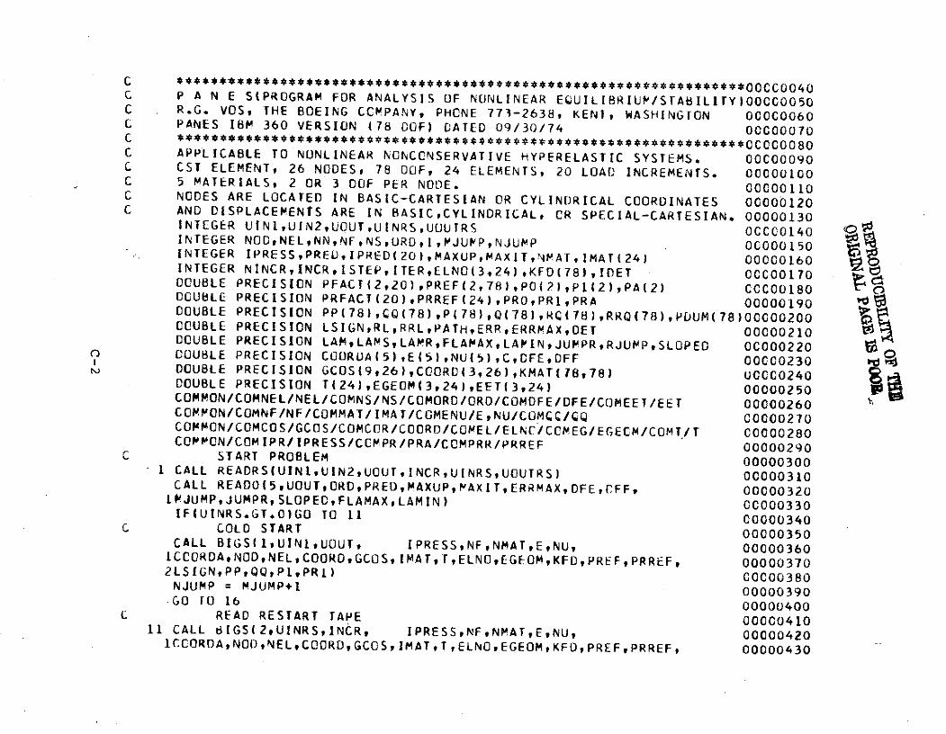
C ******************************************************************00000040C P A N E S(PROGRAM FOR ANALYSIS OF NONLINEAR EQUILIBRIUP/STABILITY)OOC0O050C R.G. VOS, THE BOEING CCMPANY, PHONE 773-2638, KENT, WASHINGTON 00000060C PANES IBM 360 VERSION (78 DOF) DATED 09/30/74 00000070C ************************************C APPLICABLE TO NONLINEAR NONCONSERVATIVE HYPERELASTIC SYSTEMS. 00C00090C CST ELEMENT, 26 NODES, 78 DOF, 24 ELEMENTS, 20 LOAD INCREMENTS. 0000100C 5 MATERIALS, 2 OR 3 DOF PER NODE. 00000110C NODES ARE LOCATED IN BASIC-CARTESIAN OR CYLINDRICAL COORDINATES 00000120C AND DISPLACEMENTS ARE IN BASIC,CYLINDRICAL, CR SPECIAL-CARTESIAN. 00000130
INTEGER UINL,UIN2,UOUT,UINRS,UOUTRS OCCCOL40INTEGER NOCONELNN,NF,NS,URDtI,JUPP,NJUMP C00000150INTEGER IPRESSPREU,IPRED(20),MAXUPMAXIT,NMATlMAT(24) 00000160INTEGER NINCR,INCR,ISTEP,ITERELNO(3,24),KFD(78),IDET OCC00170 tDOUBLE PRECISION PFACT(2,20),PREF2,78),PO(2),P(2),PA(2) CCC00000180DOUBLE PRECISION PRFACT(20),PRREF(24),PRO,PR1,PRA 00000190DOUBLE PRECISION PP(78),CQ(78),P(7 78 ),,(78),R(78),RRQ(78),PDUM(78)00000200DOUBLE PRECISION LSIGNtRL,RRLPATH,ERRERRMAX,DET 00000210DOUBLE PRECISION LAMLAMStLAMRtFLAMAXLAPINJUMPRtRJUMP SLOPED 00000220 oDOUBLE PRECISION COORVA(5),E(5),NU(5),C,CFE,DFF 00000230DOUBLE PRECISION GCOS(9,26),COORD(3,26),KMAT(18,78) 00C00240DOUBLE PRECISION T(24),EGEOM(3t24),EET(3,24) 00000250COMMON/COMNEL/NEL/COMNS/NS/COMORD/ORD/COMDFE/DFE/COMEET/EET
00000260COMMON/COMNF/NF/COMMAT/IMAT/COMENU/EUE /COMC/Q 00000270COMMON/COMCOS/GCOS/COMCOR/COORO/COMEL/ELNC/CCMEG/EGECM/COMT/T
00000280COMMON/COMIPR/IPRESS/CGMPR/PRA/COMPRR/PRREF 00000290
C START PROBLEM 000003001 CALL READRS(UINIUIN2,UOUTINCR,UINRS,UOUTRS) 00000310CALL READO(5,UOUT,ORD,PRED,MAXUP,PAXIT,ERRMAX,DFE,CFF, 00000320IMJUMP,JUMPRSLOPED,FLAMAXtLAMIN)
00000330[F(UINRS.GT.O)GO TO 11 00000340
C COLD START 00000350CALL BIGS(1,UINIUOUT, IPRESS,NF,NMAT,E,NU, 00000360ICCORDA,NOD,NEL,COORD,GCOSIMAT,T,ELNO,EGEOMKFDPREFtPRREFI 000003702LSIGN,PPQQ,P1,PRI) 00000380NJUMP = MJUMP+1 00000390GO TO 16
00000400C READ RESTART TAPE 00000410
11 CALL BIGS(2,UINRS,INCR, IPRESS,NF,NMAT,E,NU, 00000420ICCORDAtNODtNELOORGCRDGCOS,IMAT,T,ELNOEGEOM,KFDPREF,PRREF,
00000430
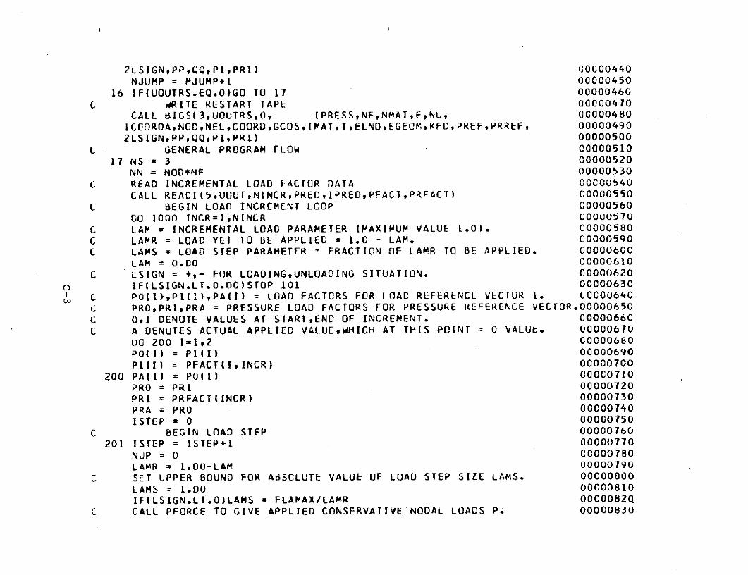
2LSIGN,PP,QQ,P1,PRI) C0000440
NJUMP = MJUMP+1 00000450
16 IF(UOUTRS.EQ.O)GO TO 17 00000460
C WRITE RESTART TAPE 00000470CALL BIGS(3,UOUTRS,0, IPRESSNFNMATE,NU, 0C000480
ICCORDANODNEL,COORDGCOS,1MATT,ELNOtEGEOM,KFDPREF,PRREF, 00000490
2LSIGNPPtQQtPIPR1) 00000500
C" GENERAL PROGRAM FLOW C0000510
17 NS = 3 00000520
NN = NOD*NF 00000530
C READ INCREMENTAL LOAD FACTOR DATA 00000540
CALL REACI(5,UOUT,NINCRPRED,IPRED,PFACT,PRFACT) C0000550
C BEGIN LOAD INCREMENT LOOP 00000560
00 1000 INCR=1,NINCR 00000570
C LAM = INCREMENTAL LOAD PARAMETER (MAXIMUM VALUE 1.0). 00000580
C LAMR = LOAD YET TO BE APPLIED = 1.0 - LAM. 00000590
C LAMS = LOAD STEP PARAMETER = FRACTION OF LAMR TO BE APPLIED. 00000600
LAM = 0.00 00000610
C LSIGN = +,- FOR LOADING,UNLOADING SITUATION. 00000620
IF(LSIGN.LT.0.0)STOP 101 00000630
C POtI),Pi(I),PA(I) = LOAD FACTORS FOR LOAC REFERENCE VECTOR 1. CC00640
C PROPR1,PRA = PRESSURE LOAD FACTORS FOR PRESSURE REFERENCE VECFOR.00000650
C O0l DENOTE VALUES AT START,END OF INCREMENT. 00000660
C A DENOTES ACTUAL APPLIED VALUE,WHICH AT THIS POINT = 0 VALUE. 00000670
00 200 1=1,2 00000680
PO(I) = P1(I) 00000690
P1(I) = PFACT(IINCR) 00000700
200 PA(I) = PO(I) 0CO00710
PRO = PRI 00000720
PRI = PRFACT(INCR) 00000730
PRA = PRO 00000740
ISTEP = 0 00000750
C BEGIN LOAD STEP 00000760
201 ISTEP = ISTEP+1 00000770
NUP = 0 00000780
LAMR = 1.00-LAM 00000790
C SET UPPER BOUND FOR ABSOLUTE VALUE OF LOAD STEP SIZE LAMS. 00000800
LAMS = 1.DO 00000810
IF(LSIGN.LT.0)LAMS = FLAMAX/LAMR 0000082Q
C CALL PFORCE TO GIVE APPLIED CONSERVATIVE'NODAL LOADS P. 00000830
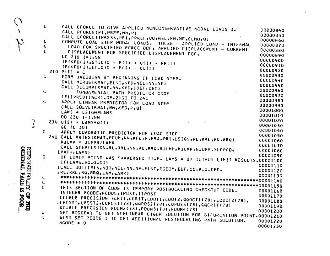
C CALL EFORCE TO GIVE APPLIED NONCCNSERVATIVE NODAL LOADS Q. C0000840CALL PFORCE(P1tPREFNN,P)00000850CALL EFORCE(IPRESSIPR1IPRREFQQtNELNNINFPELNOQ)
00000860C COMPUTE LOAD STEP NODAL LOADS. THESE = APPLIED LOAD - INTERNAL 00000870C LOAD FOR SPECIFIED FCRCE DOF, APPLIED CISPLACEMENT - CURRENT CCC0000880C DISPLACEMENT FOR SPECIFIED DISPLACEMENT DOF. 00000890DO 210 I=1,NN 00000900IF(KFDO(I).GT.O)C Z P(I) + Q(I) - pp( ) 00000910IF(KFD(I).LT.0)C = P() -) 00000920
210 P(I) = C 00000920
C FORM JACOBIAN AT BEGINNING (IF LOAD STEP. 00000930CALL MERGE(KMATELNOKFDONEL,NNNF) 00000950CALL DECOMP(KMAT,NN,KFDIDET,DET) 00000960
C FUNDAMENTAL PATH PREDICTOR CODE 00000970IF(IPRED(INCR).GE.2)GO TO 241 00000980C APPLY LINEAR PREDICTOR FOR LOAD STEP 00000990CALL SOLVE(KMATNNKFD,PQ) 00000900LAMS = LSIGN*LAMS
00001000DO 230 I=1,NN
00001010230 0(1) = LAMS*Q(1) 00001020
GC TO 301 00001030C APPLY QUADRATIC PREDICTOR FOR LOAD STEP 00001050241 CALL RATES(KMATPDUMNN,KFD,PPRAtPRItLSIGNRLRRLRC~RRQ)
00001060RJUMP = JUMPR/LAMR 00001070CALL STEP( LSIGNRL,RRL,NN,RQ,RRQ, RJUMP,MJUMP,NJUMP,SLOPED, COO010801PATHLAMS)
00001090C IF LIMIT POINT WAS TRAVERSED (I.E. LAMS = 0) OUTPUT LIMIT RESULTS.00001100IF(LAMS.EQ.O.DO) 0001110
ICALL OUTLIM(6,NOD,NEL,NN,NF,ELNO,EGEOM,EET,Q,PQCFF, 00001120
2RL,RRLRQORRQ,LMPLAMR) 00001130*C *********************0000***140
tC THIS SECTION OF CODE IS TEMPORY POSTBUCKLING CHECKOUT CODE. 00001160INTEGER BCODE,PCODE,IPOSTIIPOST 00001170OCUBLE PRECISION SCRIT,LCRITLDOTI,LDCT2,QQDCT1(78),CQDOT2(78), 00001180ILPOSTILPOST2,QOPOS1(78),QQPOS2(78),CQPOS3(78),QOCRIT(78)
00001190DOUBLE PRECISION POUM2(78)tPDUM3(78),PDUM4(78)
00001200C SET BCODE=l TO GET NONLINEAR EIGEN SOLUTION FOR BIFURCATION POINT.00001210C ALSO SET PCODE=1 TO GET ADDITIONAL PCSTBUCKLING PATH SOLUTIUN. 000012208CODE = 0 00001230
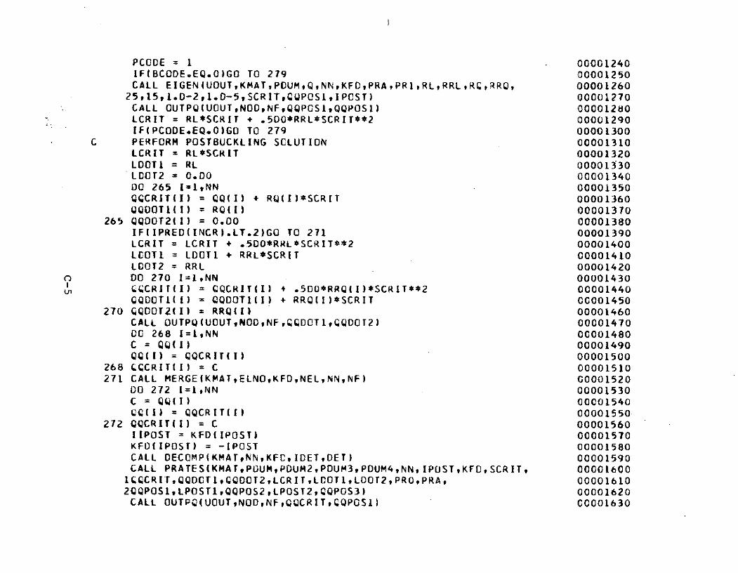
PCODE = 1 00001240IF(BCODE.EQ.O)GO TO 279 00001250CALL EIGEN(UOUTKMAT,PCUMtQNN,KFO,PRAPRI1RLRRLRC,RRQ, 0000126025,15,1.D-2,1.D-5,SCRITQQPOS1,IPCST) 00001270CALL OUTPQ(UOUT,NOO,NFQQPOSI,QQPOSI) 00001280LCRIT = RL*SCRIT + .500*RRL*SCRIT**2 00001290IF(PCODE.EQ.0)GO TO 279 00001300
C PERFORM POSTBUCKLING SCLUTION 00001310LCRIT = RL*SCRIT 00001320LDOTI = RL 00001330LOT2 = 0.00D 00001340DO 265 I=1,NN 00001350QOCRIT(I) = cQ(I) + RQ(I)*SCRIT 00001360QODOTI(I) = RQ(I) 00001370
265 QQ00OT2(I) = 0.00 00001380IF(IPRED(INCR).LT.2)GO TO 271 00001390LCRIT = LCRIT + .500*RRL*SCRIT**2 00001400LOOT1 = LDOTI + RRL*SCRIT 00001410LOOT2 = RRL 00001420DO 270 I=1,NN 00001430
t CCCRIT(I) = CQCRIT(I) + .500*RRQ(I)*SCRIT**2 00001440QQDOTI(i) = QQDOTI(I) + RRQ(I)*SCRIT 00001450
270 0QDOT2(I) = RRQ(I) 00001460CALL OUTPQ4UOUTNOD,NFC DOT1,CQD0T2) 00001470C0 268 I=1,NN 00001480C = QQ(I) 00001490QQ(I) = QQCRIT(I) 00001500
268 LCCRIT(I) = C 00001510271 CALL MERGE(KMAT,ELNO,KFDNEL,NNNF) 00001520
00 272 I=1,NN 00001530C = QQ(I) 00001540
C(1) = QQCRIT(I) 00001550272 QQCRIT(I) = C 00001560
IIPOST = KFD(IPOST) 00001570KFO(IPOST) = -IPOST 00001580CALL DECOMP(KMATtNN,KFC,IDET,DET) 00001590CALL PRATES(KMATPDUMPDUM2,PDUM3,PDUM4,NNIPOSTKFDSCRIT, 00001600ICQCRIT,QQDCT1,QQOOT2,LCRIT,LCOTILDOT2,PRO,PRA, 000016102QPOS1,LPOST1,QQPOS2,LPOST2,CQPOS3) 00001620CALL OUTPQ(UOUTNOD,NF,QQCRIT,CQPOSI) 00001630
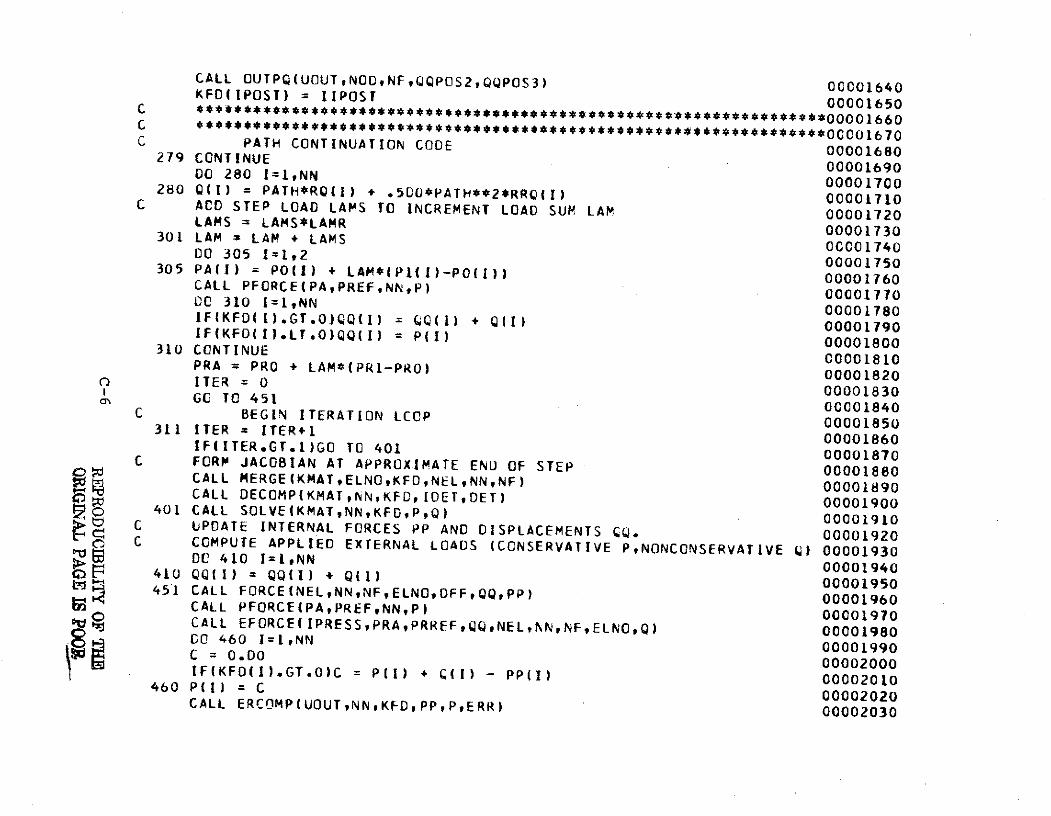
CALL OUTPQ(UOUT,NOONFQQPOS2,QQPOS3) 00C001640
KFD(IPOST) = IIPOST 00001650C 00001670
C PATH CONTINUATION CODE 00001680279 CONTINUE 00001690
DO 280 I=1,NN 00001700280 Q(I) = PATH*RQ(I) + .500*PATH**2*RRQ(I) 00001710
C ACD STEP LOAD LAMS TO INCREMENT LOAD SUM LAM 00001720LAMS = LAMS*LAMR
00001730301 LAM = LAM + LAMS 00CC0174000 305 1=1,2
00001750305 PAMl) = PO() + LAM*(PI(I)-PO(I)) 00001760CALL PFORCE(PA,PREF,NN,P) 00001770
CC 310 I=1,NN 00001780IF(KFD(I).GT.O)QQ(I) = QQ(I) + Q(I) 00001790
IF(KFO(I).LT.0)QQ(I) = P(I) 00001800310 CONTINUE 00001810PRA = PRO + LAM*(PR1-PRO) 00001820
SITER 0 00001830GC TO 451 00001840
C BEGIN ITERATION LCOP 00001850311 ITER = ITER+1 00001860
IF(ITER.GT.I)GO TO 401 00001870C FORP JACOBIAN AT APPROXIMATE END OF STEP 00001880
CALL MERGE(KMATELNOKFD,NEL,NN,NF) 00001890
CALL DECOMP(KMAT,NN,KFD,IDET,DET) 00001900C 401 CALL SOLVE(KMAT,NN,KFD,PQ) 00001910C UPDATE INTERNAL FORCES PP AND DISPLACEMENTS QQ. 00001920
o C COMPUTE APPLIED EXTERNAL LOADS (CONSERVATIVE P,NONCONSERVATIVE Q) 00001930DC 410 I=I,NN 00001940
410 QQ(I) = QQ(I) + Q(I) 00001950451 CALL FORCE(NELNNNFELNO,DFFQQ,PP)
00001960CALL PFORCE(PAPREF,NN,P) 00001970CALL EFORCE(IPRESS,PRAPRREFQQNEL,NN,NF,ELNO,Q)
00001980CO 460 I=1,NN
00001990C = 0.00
00002000IF(KFD(l).GT.O)C = P(I) + C(1) - PP(I) 00002010
460 P(I) = C 00002020CALL ERCOMP(UOUT,NNKFD,PP,P,ERR) 00002030
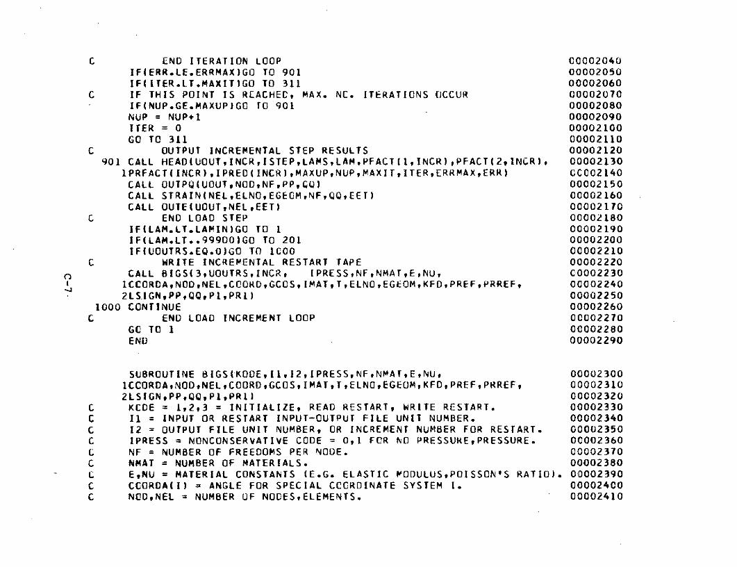
C END ITERATION LOOP C0002040IF(ERR.LE.ERRMAXIGO TO 901 00002050IF(ITER.LT.MAXIT)GO TO 311 00002060
C IF THIS POINT IS REACHEC, MAX. NC. ITERATIONS OCCUR 00002070IF(NUP.GE.MAXUP)GO TO 901 00002080NUP = NUP+1 00002090ITER = 0 00002100GO TO 311 00002110
C OUTPUT INCREMENTAL STEP RESULTS 00002120901 CALL HEADIUOUT,INCR,ISTEP,LAMS,LAM,PFACT(I,INCR),PFACT(2,INCR), 00002130
1PRFACT(INCR),IPRED(INCR),MAXUP,NUP,MAXIT,ITER,ERRMAXtERR) CC002140CALL OUTPQ(UOUT,NOD,NF,PP,CQ) 00002150CALL STRAIN(NELELNOEGEOM,NF,QQ,EET) 00002160CALL OUTE(UOUTNEL,EET) 00002170
C END LOAD STEP 00002180IF(LAM.LT.LAMIN)GO TO 1 00002190IF(LAM.LT..99900)GO TO 201 00002200IF(UOUTRS.EQ.0)GO TO 1CO0 00002210
C WRITE INCREMENTAL RESTART TAPE 00002220CALL BIGS(3,UOUTRStINCR, IPRESS,NFNMAT,EtNU, 00002230ICCORDAtNOD,NELCCORDGCOS,1MATTELNO,EGEOMKFDtPREFPRREF, 000022402LS.IGNPPtQQtPPRI) 00002250
1000 CONTINUE 00002260C END LOAD INCREMENT LOOP 0C002270
GC TO 1 00002280END 00002290
SUBROUTINE BIGS(KODEII,12tIPRESStNFNMATtE,NU. 00002300ICCORDANODtNEL,COORDGCOStIMAT,TELNOEGEOMKFDPREFPRREFt 000023102LSIGNtPPQQt,PIPRI) 00002320
C KCOE = 1,2,3 = INITIALIZE, READ RESTART, WRITE RESTART. 00002330C 11 = INPUT OR RESTART INPUT-OUTPUT FILE UNIT NUMBER. 00002340C 12 = OUTPUT FILE UNIT NUMBER, OR INCREMENT NUMBER FOR RESTART. 00002350C IPRESS = NONCONSERVATIVE CODE = 0,1 FOR NO PRESSUREPRESSURE. 0C002360C NF = NUMBER OF FREEDOMS PER NODE. 00002370C NMAT = NUMBER OF MATERIALS. 00002380C E,NU = MATERIAL CONSTANTS (E.G. ELASTIC MODULUS,POISSON'S RATIO). 00002390C CCORDAII) = ANGLE FOR SPECIAL CCORDINATE SYSTEM 1. 00002400C NODNEL = NUMBER OF NOCESELEMENTS. 00002410
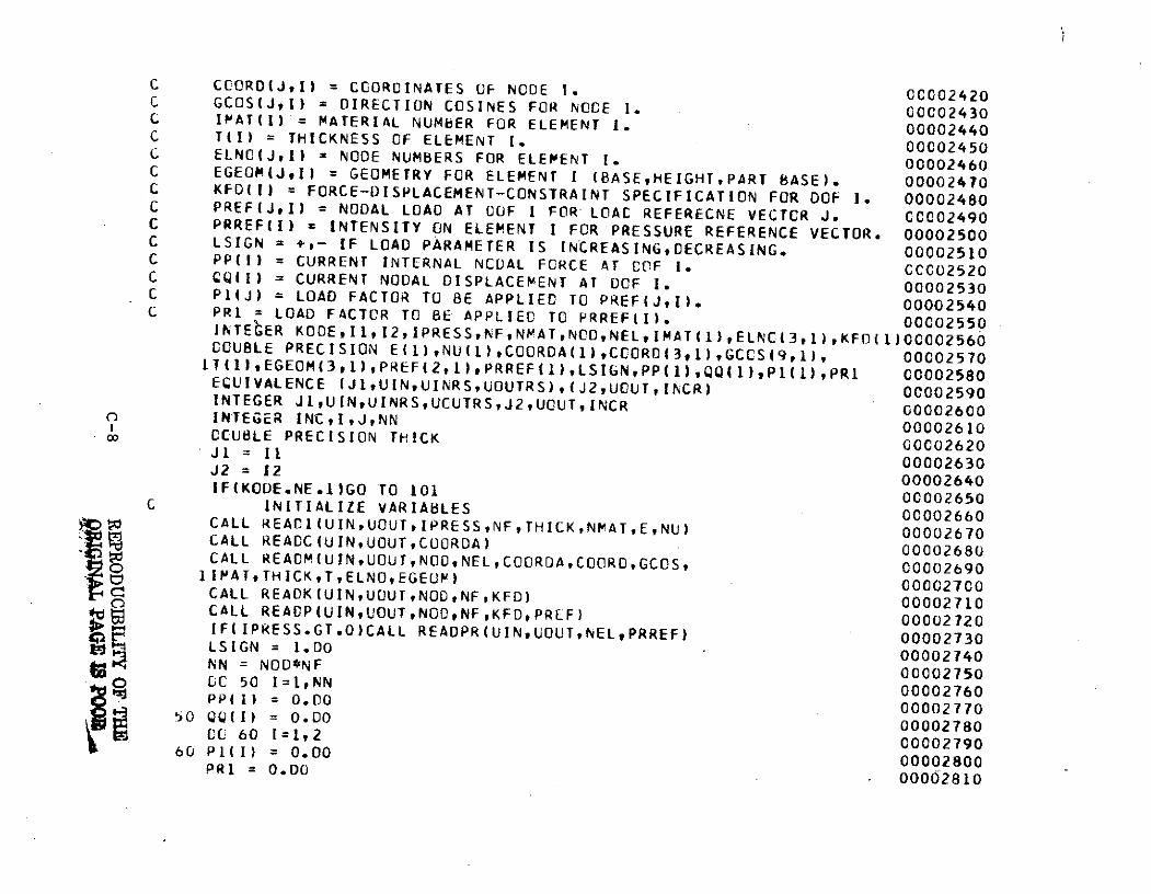
C CCORDIJ,I) = COORDINATES OF NODE 1. 00002420C GCOS(JI) = DIRECTION COSINES FOR NCDE I. 00002430C IMAT(I) = MATERIAL NUMBER FOR ELEMENT 1. 00002440C T(I) = THICKNESS OF ELEMENT I. 00002450C ELNC(JI = NODE NUMBERS FOR ELEMENT 1. 00002460C EGEOM(JIj = GEOMETRY FOR ELEMENT I (BASE,HEIGHT,PART BASE). 00002470C KFO(l) = FORCE-DISPLACEMENT-CONSTRAINT SPECIFICATION FOR DOF 1. 00002480C PREF(JI) = NODAL LOAD AT OOF I FOR LOAC REFERECNE VECTOR J. C00002490C PRREF(I) = INTENSITY ON ELEMENT I FOR PRESSURE REFERENCE VECTOR. 00002500C LSIGN = +,- IF LOAD PARAMETER IS INCREASINGOECREASING. 00002510C PP(I) = CURRENT INTERNAL NCOAL FORCE AT COF I. CCC02520C CQ(I) = CURRENT NODAL DISPLACEMENT AT DOF I. 00002530C P1(J) = LOAD FACTOR TO BE APPLIED TO PREF(J,I). 00002540C PR1 = LOAD FACTOR TO BE APPLIED TO PRREF(I). 00002550INTEeER KODE,II,I2,lPRESS,NFNMATNCDNELIMAT(1) ELNC(3tl),KFD(1)00002560
COUBLE PRECISION E(1),NU(1),COORDA(1)vCCORD(3,1),GCCS(9,1}, 00002570IT(I)IEGEOM(31),PREF(2,1)iPRREF(1),LSIGN,PP(l),QQ(1),PlI),PRI C0002580ECUIVALENCE (JlUINUINRS,UOUTRS),(J2,UOUTINCR) 00002590INTEGER JitUIN,UINRS,UCUTRS,J2,UOUT,INCR 00002600INTEGER INC,I,J,NN
00002610CCUBLE PRECISION THICK 00002620J1 = 11 00002630J2 = 12 00002630IF(KODE.NE.1)GO TO 101 00002650C INITIALIZE VARIABLES 00002660CALL REAC1(UIN,UOUTIPRESS,NF,THICK,NMAT,E,NU)
00002670rCALL READC(UIN,UOUTCOORDA) 00002680
CALL REACM(UIN,UOUT,NOD,NEL,COORDA,COORD,GCOS, 00002690IIPAT,THICK,T,ELNO,EGEON) 00002700
c CALL REAKI(UINUOUTNODNFKFD) 00002710
CALL REACP(UIN,UOUT,NOD,NF,KFD,PREF) 00002720IFilPRESS.GT.0O)CALL READPR(UINUOUT,NELPRREF) 00002730LSIGN = 1.00
00002740NN = NOD*NF 00002750
a CC 50 I=1,NN 00002760PP(l) = 0.00
0000277050 QQ(I) = 0.00 00002780
0CC 60 I=1,2 00002790
60 P1(I) = 0.00DO 00002800
PR1 = 0.00 00002810
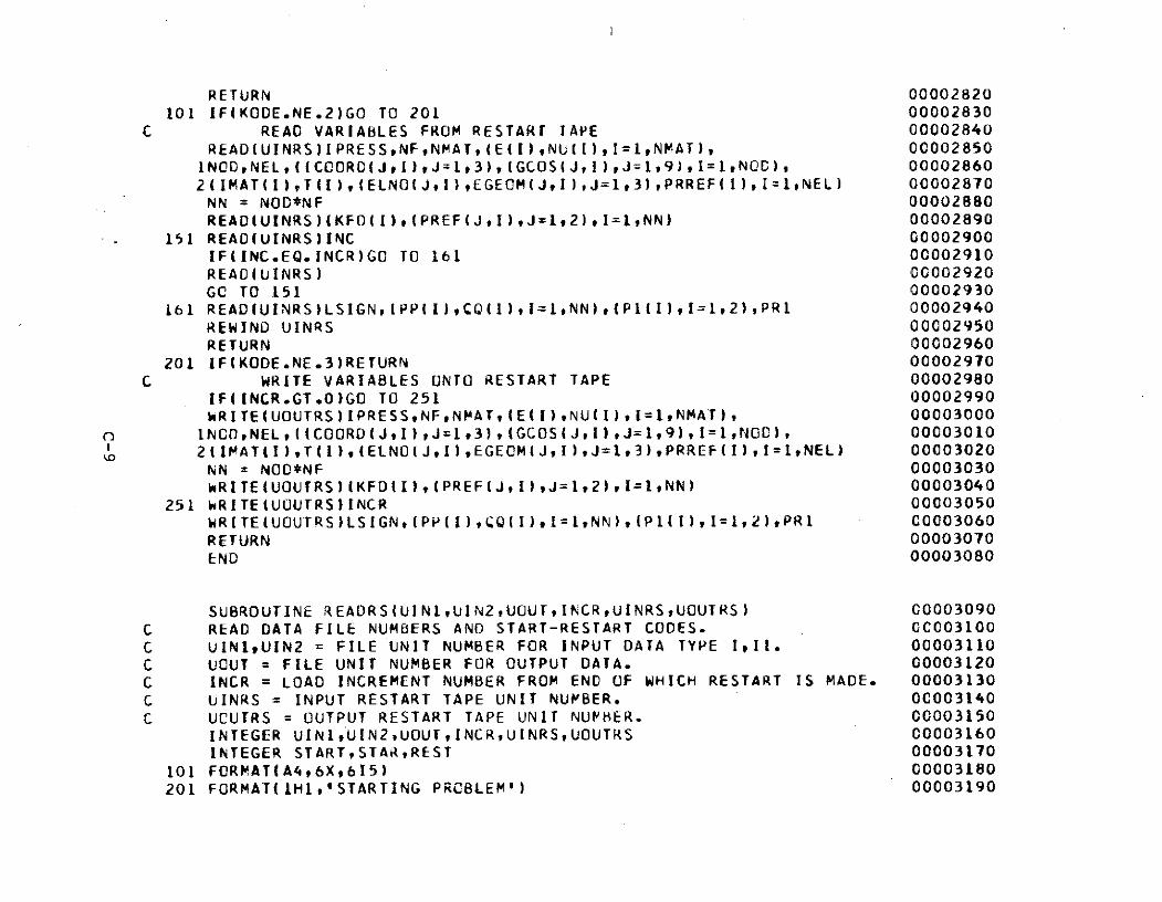
RETURN 00002820101 IF(KODE.NE.2)GO TO 201 00002830
C READ VARIABLES FROM RESTART TAPE 00002840READ(UINRS)IPRESStNF,NMAT,(E(I),NU(I)vI=1,NMAT), 00002850INCD,NEL,((CCOR0(JtI),J=1,3),(GCOS(JI),J=1,9),I=1,NOC), 00002860
2(IMAT(II)T(1),(ELNOIIJ,),EGEOM(J,I),J=1,3),PRREF(I),I=1,NEL) 00002870NN = NOD*NF 00002880READ(UINRS)(KFO(I),(PREF(J,I),J=1,2),I=1,NN) 00002890
151 READ(UINRS)INC 00002900IF(INC.EQ.INCR)GO TO 161 00002910READ(UINRS) 00002920
GC TO 151 00002930161 READ(UINRS)LSIGN,(PP(I),CQ(I),I=1,NN),(PIII)tI=1,2),PR1 00002940
REWIND UINRS 00002950RETURN 00002960
201 IF(KODE.NE.3)RETURN 00002970
C WRITE VARIABLES ONTO RESTART TAPE 00002980IF(INCR.GT.0O)GO TO 251 00002990WRITE(UOUTRS)IPRESS,NFNMAT,IE(I),NU(I),I=1,NMAT), 00003000
INCO,NEL,((COORD(J,I),J=1,3),(GCOS(J,I),J=1,9),1=1,NOD), 00003010
2tIMAT(I)T(I),T() ELNO(J,I),EGEOM(J,I),J=1,3),PRREF(),I=1,NEL) 00003020
NN = NOO*NF 00003030WRITE(UOUTRS)(KFD(I),(PREF(J,I),J=1,2),I=1NN) 00003040
251 WRITE(UOUTRS)INCR 00003050WRITE(UOUTRS)LSIGN,(PP(I),#Q(1),I=1,NN),(Pl(1),1=1,2),PR1 00003060
RETURN 00003070
END 00003080
SUBROUTINE READRS(UINL,UIN2,UOUT,INCR,UINRS,UOUTRS) 00003090
C READ DATA FILE NUMBERS AND START-RESTART CODES. 0C003100
C UIN1,UIN2 = FILE UNIT NUMBER FOR INPUT DATA TYPE 11. 00003110
C UOUT = FILE UNIT NUMBER FOR OUTPUT DATA. 00003120
C INCR = LOAD INCREMENT NUMBER FROM END OF WHICH RESTART IS MADE. 00003130
C UINRS = INPUT RESTART TAPE UNIT NUMBER. 00003140
C UCUTRS = OUTPUT RESTART TAPE UNIT NUMBER. 00003150INTEGER UINI,UIN2,UOUT,INCR,UINRS,UOUTRS 00003160
INTEGER START,STAR,REST 00003170
101 FORMAT(A4,6X,615) 00003180
201 FORMAT(IHIO1STARTING PROBLEM') 00003190
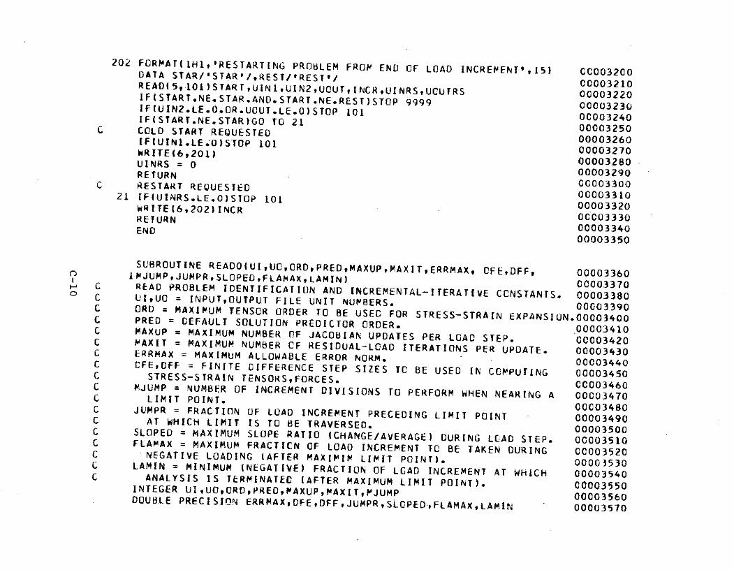
202 FORMAT(1H1,'RESTARTING PROBLEM FROM END OF LOAD INCREMENT',15) 00003200DATA STARI/STAR'/,REST/*REST'/ 00003210READ( 5 ,1o1)START,UIN1,UIN2tUUTINCR#UINRS,UCUTRS
00003220IF(START.NE.STAR.AND.START.NE.REST)STOP 9999 00003230IF(UIN2.LE.O.OR.UOUT.LE.0)STOP 101 00003240IF(START.NE.STAR)GO TO 21 00003240
C COLD START REQUESTED 00003250IF(UIN1.LE.O)STOP 101 00003260WRITE(6,201)
00003270UINRS = 0 00003280RETURN 00003290
C RESTART REQUESTED 00003300
21 IF(UINRS.LE.O)STOP 101 00003310WRITE(6,202)INCR 00003320RETURN
00003330END 00003340
00003350
SUBROUTINE READO(UIUOORDPREDMAXUPMAXITERRMAXI CFEDFFt 00003360IMJUMPtJUMPRSLOPED,FLAMAX,LAMIN) 00003370C READ PROBLEM IDENTIFICATION AND INCREMENTAL-ITERATIVE CCNSTANTS. 00003380
C UIUO = INPUT,OUTPUT FILE UNIT NUMBERS. 00003390C ORD = MAXIMUM TENSOR ORDER TO BE USED FOR STRESS-STRAIN EXPANSION.O0003400C PRED DEFAULT SOLUTION PREDICTOR ORDER. 00003410C MAXUP = MAXIMUM NUMBER OF JACOBIAN UPDATES PER LOAD STEP. 00003420C MAXIT = MAXIMUM NUMBER CF RESIDUAL-LOAD ITERATIONS PER UPDATE. 00003430C ERRMAX = MAXIMUM ALLOWABLE ERROR NORM. 00003440C CFE,DFF = FINITE CIFFERENCE STEP SIZES TO BE USED IN COMPUTING 00003450C STRESS-STRAIN TENSORS,FORCES. C0003460C MJUMP = NUMBER OF INCREMENT DIVISIONS TO PERFORM WHEN NEARING A 00003470C LIMIT POINT. 00003480C JLMPR = FRACTION OF LOAD INCREMENT PRECEDING LIMIT POINT 00003490C AT WHICH LIMIT IS TO BE TRAVERSED. 00003500C SLOPED = MAXIMUM SLOPE RATIO (CHANGE/AVERAGE) DURING LOAD STEP. 00003510C FLAMAX = MAXIMUM FRACTICN OF LOAD INCREMENT TO BE TAKEN DURING CC00003520C NEGATIVE LOADING (AFTER MAXIMIM LIMIT POINT). 00003530C LAMIN = MINIMUM (NEGATIVE) FRACTION OF LOAD INCREMENT AT WHICH 00003540C ANALYSIS IS TERMINATED (AFTER MAXIMUM LIMIT POINT). 00003550INTEGER UI,UOORDPRED,MAUPMAUP XIT,MJUMP 00003560
DOUBLE PRECISION ERRMAXDFE,DFF,JUMPRSLCPED,FLAMAX,LAMIN 00003570
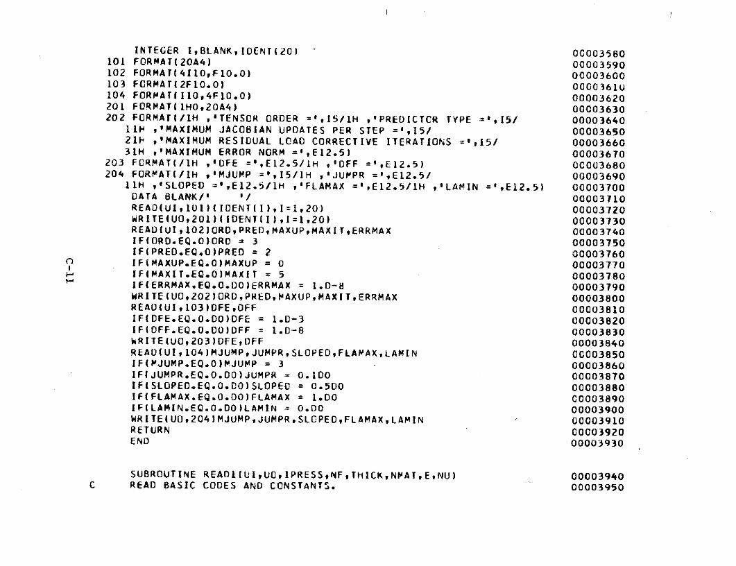
INTEGER I#BLANK,IDENT(20) 00003580101 FORMAT(2OA4) 00003590102 FORMAT(4I10F10.0) 00003600103 FCRMAT(2F10.0) 00003610104 FORMAT(I10,4F10.0) 00003620201 FORMAT(LHO20OA4) 00003630202 FORMAT(/1H ,'TENSOR ORDER =,IS5/1H ,'PREDICTCR TYPE =,15/ 00003640
11H ,'MAXIMUM JACOBIAN UPDATES PER STEP =',15/ 0000365021H ,'MAXIMUM RESIDUAL LOAD CORRECTIVE ITERATIONS =,151/ 0000366031H ,'MAXIMUM ERROR NORM =',E12.5) 00003670
203 FCRMAT(/IH ,'DFE =',E12.5/IH ,'DFF =',E12.5) 00003680204 FORPAT(/IH IMJUMP =',IS/1H ,'JUPPR =',E12.5/ 00003690
11H '*SLOPED =',E12.5/1H O'FLAMAX =',E12.5/1H 9,LAMIN =',E12.5) 00003700DATA BLANK/' ' 00003710REAO(UI,101)(IDENTII),I=1,20) 00003720WRITE(UO,201)(IDENT(I),I=1,20) 00003730READ(UI,102)ORDPRED,MAXUPMAXITtERRMAX 00003740IF(ORD.EQ.O)ORD = 3 00003750IF(PREDEQ.0O)PRED = 2 00003760IFiMAXUP.EQ.O)MAXUP = 0 00003770IF(MAXIT.EQ.O)MAXIT = 5 00003780IF(ERRMAX.EQ.0.D0)ERRMAX = 1.0-8 00003790WRITE(UO,202)ORDPRED,MAXUPMAXITERRMAX 00003800READ(UI,103)DFE,DFF 00003810IF(DFE.EQ.O.DO)DFE = 1.0-3 00003820IF(DFF.EQ.0.D0)DFF = 1.0-8 00003830WRITE(UO,203)DFE,DFF 00003840READ(UI,104)MJUMPJUMPR,SLOPED,FLAAX,LAMIN 00003850IF(PJUMP.EQ.O)MJUMP = 3 00003860IFfJUMPR.EQ.0.DO)JUMPR = 0.100 00003870IF(SLOPED.EQ.0.00)SLOPED = 0.5DO 00003880IF(FLAMAX.EQ.0.O0)FLAMAX = I.DO 00003890IF(LAMIN.EQ.O.DO)LAMIN = 0.00 00003900WRITE(UO,204)MJUMP,JUMPR,SLCPEO,FLAMAX,LAMIN 00003910RETURN 00003920END 00003930
SUBROUTINE READL(UIUOIPRESSNFTHICK,NPAT,EtNU) 00003940C READ BASIC CODES AND CONSTANTS. 00003950
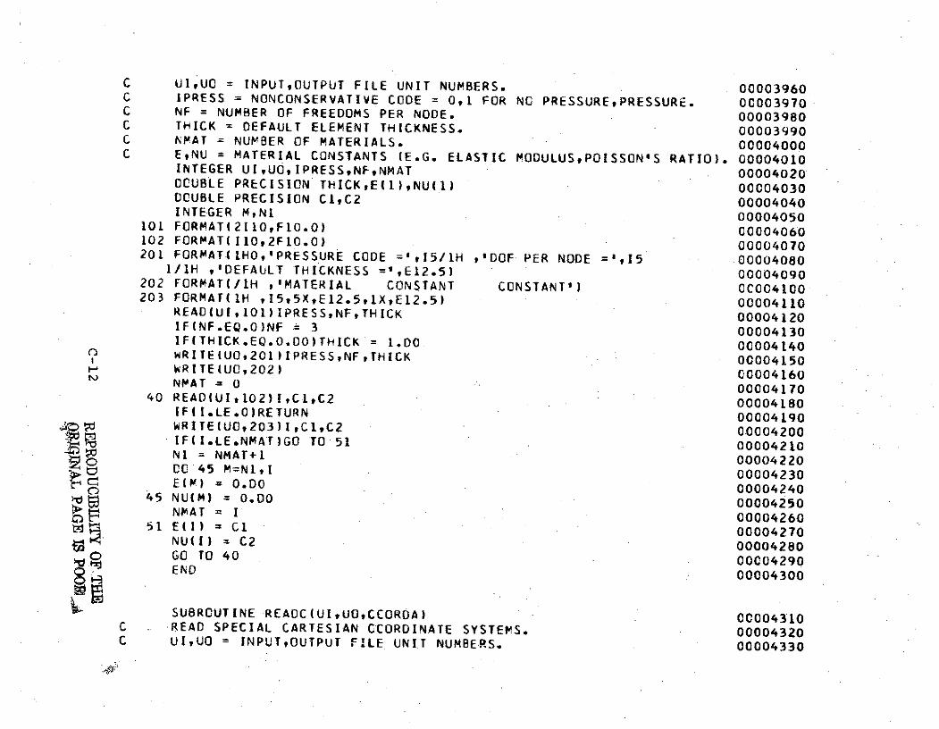
C UI,UO = INPUTeOUTPUT FILE UNIT NUMBERS. 00003960C IPRESS = NONCONSERVATIVE CODE = 0,1 FOR NO PRESSUREtPRESSURE. 00003970C NF = NUMBER OF FREEDOMS PER NODE. 00003980C THICK = DEFAULT ELEMENT THICKNESS. 00003990C NMAT NUMBER OF MATERIALS. 00004000C E,NU = MATERIAL CONSTANTS (E.G. ELASTIC MODULUSPOISSON'S RATIO). 00004010
INTEGER UI,UO,IPRESSNF,NMAT 00004020DOCUBLE PRECISION THICK,E(1),NU(1) 00004030DOCUBLE PRECISION CI,C2 00004040INTEGER M,N1 00004050
101 FORMAT(2110,F10.0) 00004060102 FORMAT(II02F10.0) 00004070201 FORMAT(IHO,'PRESSURE CODE ='I,5/1H PDOF PER NODE =I,15 00004080
1/1H ,'DEFAULT THICKNESS =',E12.5) 00004090202 FORMAT(/1H ,'MATERIAL CONSTANT CONSTANT') Co004100203 FORMAT1H ,15,5X,E12.5qIXE12.S) 00004110
READ(UI,101)IPRESS,NF,THICK 00004120IF(NF.EQ.O)NF = 3 00004130IF(THICK.EQ.O.DO)THICK = 1.DO. 00004140WRITE(UO,201)IPRESS,NFTHICK 00004150WRITE(U0,202) 00004160NMAT = 0 00004170
40 READIUIl02)I,CItC2 00004180IFiI.LE.0)RETURN 00004190WRITE(UO,203)I,C1,C2 00004200IF(I.LE.NMAT)GO TO 51 00004210NI = NMAT+1 00004220DC 45 M=N1,I 00004230EL) = 0.00 00004240
) 45 NU(M) = 0.DO 00004250NMAT = I
0000426051 E(I) = C1 00004270
NUL() = C2 00004280O GO TO 40 00004290
END 00004300
SUBROUTINE READC(UIUOCCORDA) 00004310C READ SPECIAL CARTESIAN CCORDINATE SYSTEMS. 00004320C UI,UO INPUT,OUTPUT FILE UNIT NUMBE-RS. 00004330
C CCORDA(I) = ANGLE FOR SPECIAL COCROINATE SYSTEM I. CC004340INTEGER UI,UO 00004350DOUBLE PRECISION COORDA(1) 00004360INTEGER I 00004370CCUBLE PRECISION ANGLE,F 00004380
101 FORMAT(II0,FI0.0) 00004390201 FORMAI(//IHI,'CARTESIAN COORDINATE SYSTEMS DEFINED'/ 00004400
11i ,'NUMBER X-AXIS ANGLE') 00004410202 FORMAT(1H ,15,5X,FIO.4) 00004420
F = 3.14159265358979300/180.DO 00004430WRITE(U0O201) GCC0444000 5 1=1,5 00004450
5 COORDA(I) = 0.DO 0000446010 READ(UI,101)I,ANGLE 00004470
IFII.LE.O)RETURN 00004480WRITE(UOt202)I1ANGLE 00004490COORDACI) = ANGLE*F 00004500GO TO 10 00004510END 00004520
SUBROUTINE READM(UI,UO,NOD,NEL,CCORDAtCCORDGCOS, 00004530IIMAT,iHICK,T,ELNO,EGEOM) 00004540
C READ MESH DATA. 00004550C UIUO = INPUTOUTPUT FILE UNIT NUMBERS. 00004560C NCD,NEL = NUMBER OF NOCES,ELEMENTS. 00004570C CCORDA(I) = ANGLE FOR SPECIAL COORDINATE SYSTEM I. 00004580C CCORD(JI) = COORCINATES FOR NODE I. 0C004590C GCOS(JlI) = DIRECTION COSINES FOR NODE 1. 00004600C IVAT(I) = MATERIAL NUMBER FOR ELEMENT 1. 00004610C THICK = DEFAULT THICKNESS. 00004620C T(I) = THICKNESS OF ELEMENT I. 00004630C ELNO(JI) = NODE NUMBERS FOR ELEMENT I. 00004640C EGEOM(J,I) = GEOMETRY FOR ELEMENT I (BASE,HEIGHTPART BASE). 00004650
INTEGER UIUO,NOD,NEL,IMAT(1),ELNC(3,1) 00004660CCUBLE PRECISION COORDAII),CCORD(3,1),THICK,VLENTH,VDOT 00004670DOUBLE PRECISION GCOS(3,3,1),EGEOM(3,1),T(1) 00004680INTEGER IJM,LCOORD,DCCORD,NI,N2,N3 00004690DOUBLE PRECISION F,ANGLE,X,Y,Z,R,TT,8,81,H,L31,A,V21(3),V31(3) 00004700
101 FORMAT(215,3F10.0,15) 00004710
102 FORMAT(215,F10.0,315) C0004720
201 FORMAT(IH1,'** NODE ***/IH ,' NO. I.D. LCOCRD X (R)', 0CC0473017X'Y (THETA) z DCOORD*) 00004740202 FORMAT(IH 9215,1X,I5,2X,EI2.5,1X,EI2.5,1X,E2.5,X,15) 0C004750
203 FORMAT(1HI,' ELEMENT '/ 00004760IIH ,' NO. 1.0. MATERIAL THICKNESS',4x, 000047702'NODE 1 NODE 2 NODE 3 AREA') 00004780204 FORMATIH .2 15,5X15tSX,E2.4X,2.4X,15X,15,X,I5,5X,E12.4) 00004790F = 3.14159265358979300/180.DO
00004800WRITE(UO,201)
00004810NCO = 0
000048206 REAO(UI,101)I,LCOOROX,Y,Z,DCCORD 00004830
IF(I.LE.O)GO TO 150 00004840NOD = NOD+1
00004850WRITE(UOt202)NOD,[,LCOCRO,X,Y,ZtCCOR
CC004860COURD(3,NOD) = Z 00004870IF(LCOORD.EQ.0)GO TO 7 00004880ANGLE = Y*F
00004890Y = X*DSIN(ANGLE)
00004900X = X*DCOS(ANGLE)
000049107 CCORD(1,NOO) = X 00004920
CCORO(2,NOD) = Y 00004930IF(DCOORD-1)13,12,11
0000494011 ANGLE = COORDA(DCOURD) 00004950
GCOS(1,1,NOD) = OCOS(ANGLE) 00004960GCOS(1,2,NOD) = DSIN(ANGLE) 00004970GO TO 100
0000498012 R = DSQRT(X**2 + Y**2) 00004990
IF(R.EQ.0.D0)GO TO 13 00005000GCOS(1,1,NOD) = X/R 00005010GCOS(1,2,NOD) = Y/R 00005020GO TO 100
0000503013 GCOS(LlitNOD) = 1.DO 00005040
GCOS(1,2,N0) = 0.UO 00005050100 GCOS(1,3,NOD) = 0.00 00-005060GCOS(2,1,NOD) = -GCOS(1,2,NOD) 00005070GCOS(2,2,NO) = GCOS(1,1,NOD) 0C005080GCOS(2,3,NCD) = 0.00 00005090GCOS(3,1,NOD) = 0.00 00005100GCOS(3,2,NOD) = 0.00 00005110
GCOS(3,3,NOD) = 1.00 00005120GO rO 6 00005130
150 WRITE(UO,203) 00005140NEL = 0 00005150
151 READ(UI,102)I,M,TTNlN2,N3 C0005160IFII.LE.O)GO TO 250 00005170IF(TT.EQ.0.DO)TT = THICK 00005180NEL = NEL+1 00005190IMAT(NEL) = M 00005200T(NEL) = TT 00005210CC 170 J=1,3 00005220V21(J) = CCORD(JN2) - CCORD(J,NI) 00005230
170 V31(J) = COORD(JN3) - CCORD(J,NL) 00005240B = VLENTH(V21) 00005250L31 = VLENTHIV31) 0000526061 = VDOT(V21,V31)/B 00005270H = DSQRT(L31**2 - 81**2) 00005280A = .500*B*H 00005290EGEOM(t1NEL) = B 00005300EGEOM(2,NEL) = H 00005310EGEOM(3,NEL) = 81 00005320
Ln 200 WRITE(UO,204)NEL,IM,TT,NIPN2,N3,A 00005330ELNOLtINEL) = NI 00005340ELNO(2,NEL) = N2 00005350ELNO(3,NEL) = N3 00005360GO TO 151 00005370
250 RETURN 00005380END 00005390
SUBROUTINE READK(UIlUONODtNF,KFD) 00005400C READ SPECIFIED FORCE-DISPLACEMENT-CONSTRAINT DEGREES OF FREEDOM. 00005410C UI,UO = INPUT,OUTPUT FILE UNIT NUMBERS. 00005420C NCD = NUMBER OF NODES. 00005430C NF = NUMBER OF FREEDOMS PER NODE. 00005440C KFD(I) = FORDE-DISPLACEPENT-CONSTRAINT SPECIFICATION FOR DOF I. 00005450
INTEGER UIUG,NODNFKFC(1) 0CC05460INTEGER ISTOR(4),JSTOR(4),KSTOR(4),LSTOR(4) 00005470INTEGER ItJKLMtNNJLCC,LLOC 00005480
101 FORMAT(4(415)) 00005490
201 FORMAT(//H1,'SPECIFIEO FORCE-DISPLACEMENT-CONSTRAINT COF' C000055001/IH ,'NODE I.D. COMPONENT NODE I.D. CCMPONENT') 00005510
202 FCRMATIIH ,15,6X,15,6X,15,6X,15) 00005520NN = NOD*NF 00005530WRITE(UO,201) 00005540
C SET DEFAULT CODES TO SPECIFIED FORCE. 0000555000 5 I=1,NN 00005560
5 KFC(I) = I 0000557010 READ(UI,101)(ISTOR(K),JSTORIK),KSTCR(K),LSTOR(K),K=1,4) 00005580
DO 12 M=1,4 00005590IF(ISTOR(M).NE.C)GO TO 13 00005600
12 CONTINUE 00005610GO TO 51 00005620
13 00 20 M=1,4 00005630I = ISTOR(M) 00005640IF(I.LE.O)GO TO 20 00005650J = JSTOR(M) 00005660K = KSTOR(M) 00005670L = LSTOR(M) 00005680WRITE(UO,202)ItjK,L 00005690IF(K.EQ.O)K = I C00005700IF(L.EQ.0)L = -J 00005710JLOC = NF*tI-1) + J 00005720LLOC = L 00005730IF(L.LT.O)LLOC = -L 00005740LLOC = NF*(K-1) +.LLOC 00005750IF(L.LT.O)LLOC = -LLOC 00005760KFDIJLOC) = LLOC 00005770
20 CONTINUE 00005780GO TO 10 00005790
51 RETURN OC0080058END 00005810
SUBROUTINE REAOPIUI,UO,NOD,NF,KFO,PREF) 00005820C READ LOAD REFERENCE CURVES. 00005830C LI,UO = INPUT,OUTPUT FILE UNIT NUMBERS. 00005840C NCO = NUMBER OF NODES. 00005850C NF = NUMBER OF FREEDOMS PER NODE. 00005860C KFD(I) = FORCE-DISPLACEMENT-CONSTRAINT SPECIFICATION .FOR-"DOF I.. 00005870
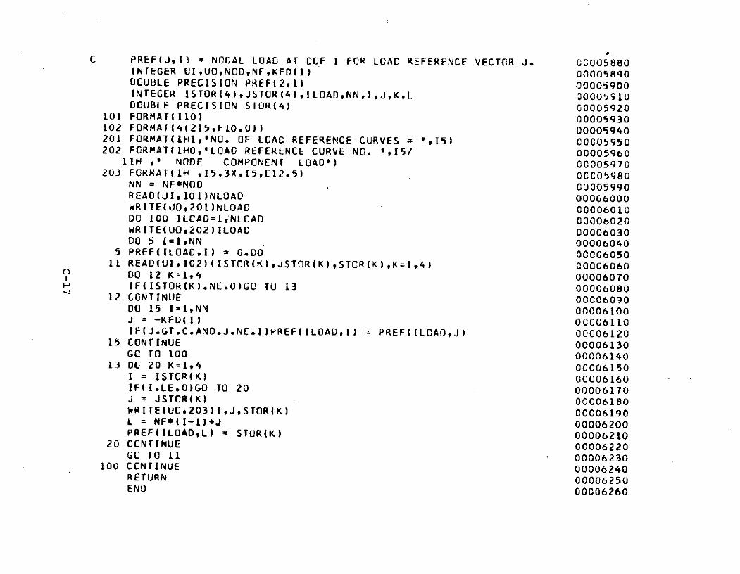
C PREF(JIl) = NODAL LOAD AT CGF I FOR LOAD REFERENCE VECTOR J. 00005880INTEGER UIUONODNFKFD(l) 00005890DOUBLE PRECISION PREF(2,1) 00005900INTEGER ISTOR(4),JSTOR(4),lLOADNNtl,J,KL 00005910DOUBLE PRECISION STOR(4) C0005920
101 FORMAT(I10) 00005930102 FORMAT(4(2I5,FIO.0)) 00005940201 FORMAT(IHI,'NO. OF LOAD REFERENCE CURVES = ',15) COC05950202 FORMAT(1HO'LOAD REFERENCE CURVE NC. ',I5/ 00005960
11H ,' NODE COMPONENT LOAD') 00005970203 FORMAT(1H ,I5,3X,15,E12.5) 0CC05980
NN = NF*NOO 00005990READ(UI,1OI)NLOAD 00006000WRITE(UO,201)NLOAD 00006010DO 100 ILOAD=L1NLOAD 00006020WRITE(UO,202)ILOAD 00006030DO 5 I=1,NN 00006040
5 PREF(ILOAD,I) = 0.00 0000605011 READ(UI,102)(ISTOR(K),JSTOR(K),STCR(K),K=1,4) 00006060
DO 12 K=1,4 00006070IF(ISTOR(K).NE.O)GO TO 13 00006080
12 CONTINUE 0000609000 15 I=1,NN 00006100J = -KFD(I) 00006110IF(J.GT.0.AND.J.NE.I)PREFILOAD,I) = PREF(ILCAD,J) 00006120
15 CONTINUE 00006130GO TO 100 00006140
13 DC 20 K=1,4 00006150I = ISTORK) 00006160IF(I.LE.0)GO TO 20 00006170J = JSTOR(K) 00006180WRITE(UO,203)I,JtSTOR(K) 00006190L = NF*(I-11+J 00006200PREF(ILOAD,L) = STOR(K) 00006210
20 CONTINUE 00006220GC TO 11 00006230
100 CONTINUE 00006240RETURN 00006250ENO 00006260

SUBROUTINE READPR(UI,UCNELPRREF) 00006270C READ PRESSURE LOAD REFERENCE CURVE* 00006280C UI,UO = INPUT,OUTPUT FILE UNIT NUMBERS. 00006290C NEL z NUMBER OF ELEMENTS. 00006300C PRREF(I) = INTENSITY ON ELEMENT I FOR PRESSURE REFERENCE VECTOR. 00006310
INTEGER UItUOtNEL 00006320CGUBLE PRECISION PRREF(1) 00006330INTEGER ISTOR(4),ILOADIK 00006340DOUBLE PRECISION STOR(4) 00006350
101 FORMAT(I10) 00006360102 FORMAT(4(110,F10.O)) 00006370201 FORMAT(IHI,NO. OF PRESSURE LOAD REFERENCE CURVES =',15) 00006380202 FORMAT(IHO,'PRESSURE LOAD REFERENCE CURVE NO.',15/ 00006390
11H 91ELEMENT PRESSURE') 00006400203 FORMAT(lH ,15,3XE12.5) 00006410
READ(UI,101)NLOAD 00006420WRITE(UO,2O1)NLOAD 00006430OC 100 ILOAD=1,NLOAD 00006440WRITE(UO,202)ILOAD 0000645000 5 I=1,NEL 00006460
5 PRREF(I) = 0.00 0000647011 READ(UI,102)(ISTORIK),STORIK),K=1,4) 00006480
00 12 K=1,4 00006490IFIISTOR(K).NE.O)GO TO 13 00006500
12 CONTINUE 00006510GO TO 100 00006520
13 DO 20 K=1,4 00006530I = ISTOR(K) 00006540IF(I.LE.0)GO TO 20 00006550WRITE(UO9203)ISTOR(K) 00006560PRREF(I) = STOR(K) 00006570
20 CONTINUE 00006580GO TO 11 00006590
100 CONTINUE 00006600RETURN 00006610END 00006620
SUBROUTINE REAOI(UIUONINCRiPREDOIPREi PFACTPRFACT) 00006630
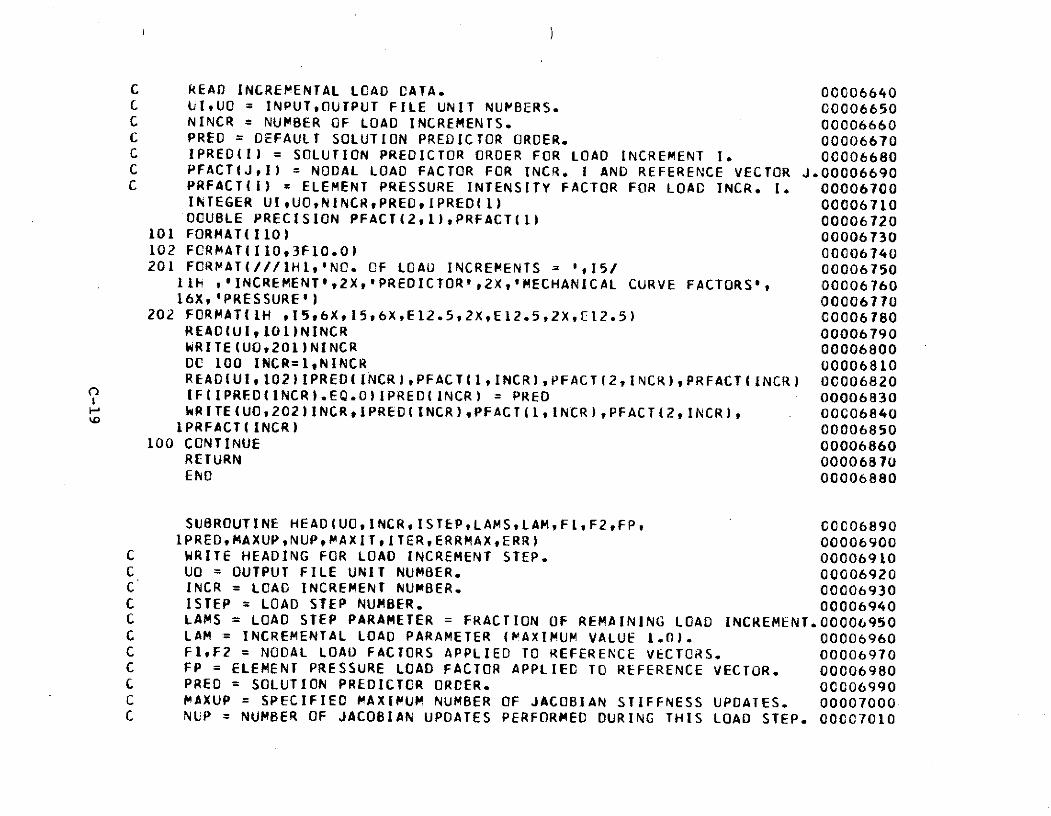
C READ INCREMENTAL LOCAD DATA. 0006640C UIUO = INPUTtOUTPUT FILE UNIT NUMBERS. 00006650C NINCR = NUMBER OF LOAD INCREMENTS. 00006660C PRED = DEFAULT SOLUTION PREDICTOR ORDER. 00006670C IPREO(I) = SOLUTION PREDICTOR ORDER FOR LOAD INCREMENT I. 0C006680C PFACTIJI) = NODAL LOAD FACTOR FOR INCR. I AND REFERENCE VECTOR J.00006690C PRFACT(I) = ELEMENT PRESSURE INTENSITY FACTOR FOR LOAD INCR. I. 00006700
INTEGER UIUONINCRvPREDIPRED(1) 00006710DOUBLE PRECISION PFACT(2,1),PRFACT(l) 00006720
101 FORMAT(I10) 00006730102 FCRMAT(I10,3F10.0) 00006740201 FCRMAT(///IHI'NO. OF LOAD INCREMENTS = ',15/ 00006750
11H ,'INCREMENT',2Xt'PREDICTOR',2X,tMECHANICAL CURVE FACTORS', 0000676016X,'PRESSURE') 00006770
202 FORMAT(IH ,lI56X,15,6XE12.5,2XE12.5,2X,CI2.5) C0006780REAO(UI,IO1)NINCR 00006790WRITE(UO,201)NINCR 00006800DC 100 INCR=1,NINCR 00006810READ(UIl102)IPRED(INCR),PFACT(I,INCR),PFACT(2,INCR),PRFACT(INCR) 0C006820IF(IPRED(INCR).EQ.OIPRED(INCR) = PRED 00006830WRITE(UO,202)INCRIPRED(INCR),PFACT(1,INCR),PFACT(2,lNCR), 000068401PRFACT(INCR) 00006850
100 CONTINUE 00006860RETURN 00006870END 00006880
SUBROUTINE HEAD(UO,INCRISTEPtLAMSLAM,FI,F2,FPt 00C06890IPREDMAXUPNUPMAXITITERERRMAXERR) 00006900
C WRITE HEADING FOR LOAD INCREMENT STEP. 00006910C UO = OUTPUT FILE UNIT NUMBER. 00006920C INCR = LOAD INCREMENT NUMBER. 00006930C ISTEP = LOAD STEP NUMBER. 00006940C LAMS = LOAD STEP PARAMETER = FRACTION OF REMAINING LOAD INCREMENT.00006950C LAM = INCREMENTAL LOAD PARAMETER (MAXIMUM VALUE 1.0). 00006960C FI,F2 = NODAL LOAD FACTORS APPLIED TO REFERENCE VECTORS. 00006970C FP = ELEMENT PRESSURE LOAD FACTOR APPLIED TO REFERENCE VECTOR. 00006980C PRED = SOLUTION PREDICTOR ORDER. 0C006990C MAXUP = SPECIFIED MAXIMUM NUMBER OF JACOBIAN STIFFNESS UPDATES. 00007000C NUP = NUMBER OF JACOBIAN UPDATES PERFORMED DURING THIS LOAD STEP. 00CC7010
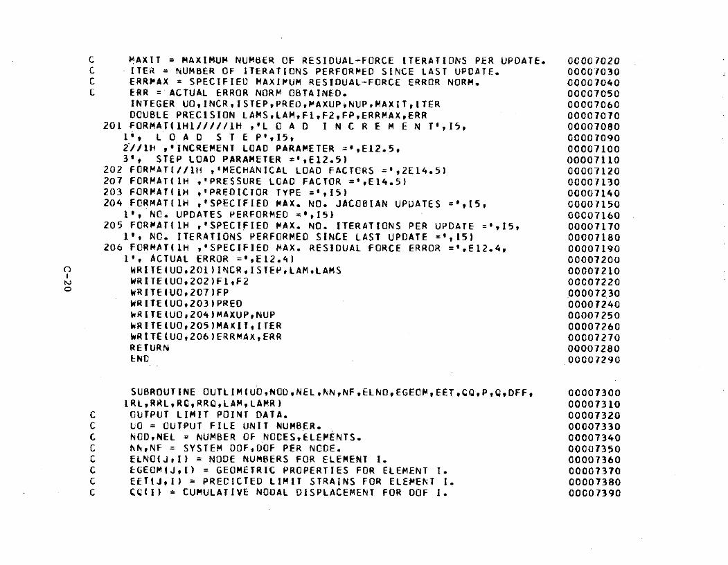
C MAXIT = MAXIMUM NUMBER OF RESIDUAL-FORCE ITERATIONS PER UPDATE. OC007020C ITER = NUMBER OF ITERATIONS PERFORMED SINCE LAST UPDATE. 00007030C ERRMAX = SPECIFIED MAXIMUM RESIDUAL-FORCE ERROR NORM. 00007040C ERR = ACTUAL ERROR NORM OBTAINED. 00007050
INTEGER UO,INCR,ISTEPPREO,MAXUPNUNUPMAXIT,ITER 00007060DOUBLE PRECISION LAMS,LAM,FI,F2tFP,ERRMAXERR 00007070
201 FORMAT(1H1/////IH ,'L 0 A D I N C R E M E N T',I5, 000070801', L 0 A D S T E P'1I5, 000070902II//1H ,INCREMENT LOAD PARAMETER =0,E12.5, 000071003', STEP LOAD PARAMETER =',E12.5) 00007110
202 FORMAT(//1H ,'MECHANICAL LOAD FACTORS =',2E14.5) 00007120207 FORMAT(IH ,'PRESSURE LCAD FACTOR =',E14.5) 00007130203 FORMAT(1H ,'PREDICTOR TYPE =',15) 00007140204 FORMAT(IH ,'SPECIFIED MAX. NO. JACOBIAN UPDATES =',15, 00007150
1', NO. UPDATES PERFORMED =,15) 00C007160205 FORMAT(1H ,'SPECIFIED MAX. NO. ITERATIONS PER UPDATE =',15, 00007170
1', NO. ITERATIONS PERFORMED SINCE LAST UPDATE =',15) 00007180206 F*CRMAT(IH ,'SPECIFIED MAX. RESIDUAL FORCE ERROR =',E12.4, 00007190
1', ACTUAL ERROR =',E12.4) 00007200O WRITEIUO,201)INCR,ISTEPLAM,LAMS 00007210
WRITE(UO*202)FI,F2 00007220o WRITE(UO,207)FP 00007230
WRITE(UO203)PRED 00007240WRITE(UO,204)MAXUP,NUP 00007250WRITE(UO,205)MAXITITER 00007260WRITE(UO,206)ERRMAXtERR 00007270RETURN 00007280END 00007290
SUBROUTINE OUTLIM(UO,NOD,NEL,NN,NF,ELN0,EGECMtEET,CQ,P,Q,DFF, 00007300LRL,RRRR RRQ,LAM,LAMR) 00007310
C OUTPUT LIMIT POINT DATA. 00007320C UO = OUTPUT FILE UNIT NUMBER. 00007330C NOD,NEL = NUMBER OF NOCESELEMENTS. 00007340C NNhNF = SYSTEM DOF,DOF PER NODE. 00007350C ELNO(JeI) = NODE NUMBERS FOR ELEMENT I. 00007360C EGEOM(JI) = GEOMETRIC PROPERTIES FOR ELEMENT I1 00007370C EET(J,I) = PRECICTED LIMIT STRAINS FOR ELEMENT I. 00007380C C.(I) = CUMULATIVE NODAL DISPLACEMENT FOR DOF 1. 00007390
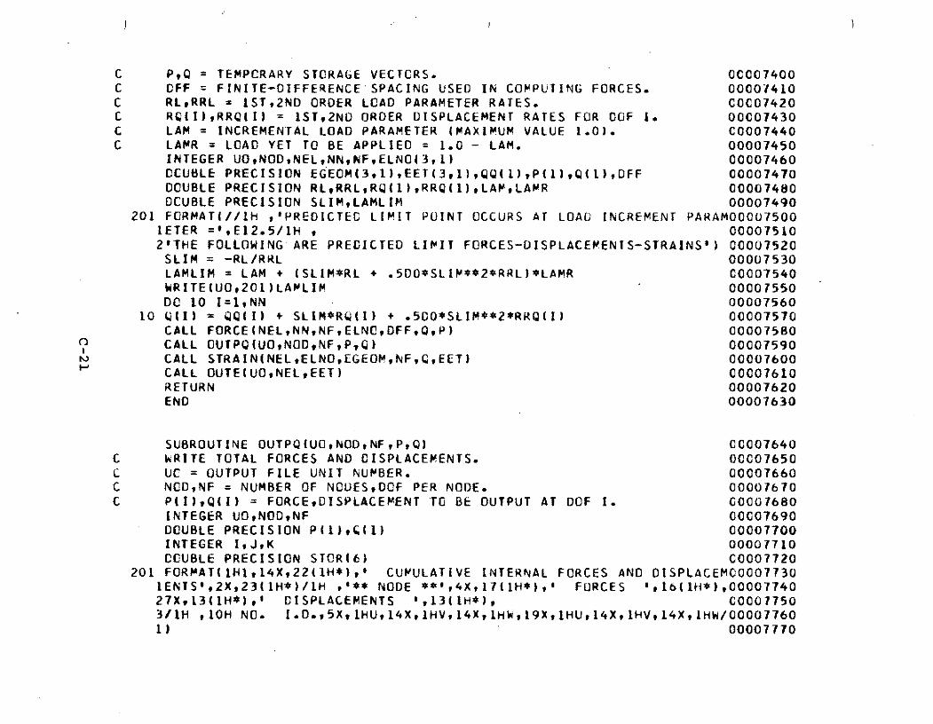
C P,Q = TEMPORARY STORAGE VECTCRS. OC007400C OFF = FINITE-DIFFERENCE SPACING USED IN COMPUTING FORCES. 00007410C RL,RRL = IST,2ND ORDER LOAD PARAMETER RATES. 00007420C RC(I),RRQ(I) = 1ST,2ND ORDER DISPLACEMENT RATES FOR ODF I. 00007430C LAM = INCREMENTAL LOAD PARAMETER (MAXIMUM VALUE 1.0). C0007440C LAMR = LOAD YET TO BE APPLIED = 1.0 - LAM. 00007450
INTEGER UOtNODNELNNNF,ELNO(3,1) 00007460DCUBLE PRECISION EGEOM(3,l),EET(3,1)tQQ(1),P(1),Q(l),DFF 00007470DOUBLE PRECISION RLRRL,RQ(1),RRQ(1),LAMtLAMR 00007480DCUBLE PRECISION SLIM,LAMLIM 00007490
201 FORMAT(//I ,'PREDICTEC LIMIT POINT OCCURS AT LOAD INCREMENT PARAMOO007500IETER =',E12.5/IH , 000075102'THE FOLLOWING ARE PREDICTED LIMIT FORCES-DISPLACEMENTS-STRAINS') 00007520SLIM = -RL/RRL 00007530LAMLIM = LAM + (SLIM*RL + .500*SLIM**2*RRL)*LAMR C0007540WRITE(UO,201)LAMLIM 00007550DC 10 I=1,NN 00007560
10 Q(I) = QQ(I) + SLIM*RQ(I) + .5O*SLIM**2*RRQ(I) 00007570CALL FORCE(NELNNNFtELNO,DFFQP) 00007580CALL OUTPQ(UONODNFP,Q) 00007590CALL STRAIN(NELtELNO,EGEOM,NF,qEET) 00007600CALL OUTE(UO,NELEET) 00007610RETURN 00007620END 00007630
SUBROUTINE OUTPQ(UOtNODNFPQ) 00007640C WRITE TOTAL FORCES AND DISPLACEMENTS. 00007650C UC = OUTPUT FILE UNIT NUMBER. 00007660C NCDNF = NUMBER OF NOUESDOF PER NODE. 00007670C P(I)Q(I) = FORCE,DISPLACEMENT TO BE OUTPUT AT DOF 1. 00007680
INTEGER UONODNF 00007690DOUBLE PRECISION P(1),s(1) 00007700INTEGER IJqK 00007710COUBLE PRECISION STOR16) 00007720
201 FORMAT(IHI,14Xt22(1H*),' CUMULATIVE INTERNAL FORCES AND OISPLACEM000077301ENTS',2X,23(1H*)/IH ,'** NODE **',4X,17(H*),O FORCES ',16(IH*),0000774027X,13(IH*),' DISPLACEMENTS ',13(IH*), C00077503/1H ,10H NO. I.D.,5XvIHU,14X,1HV,14X,1HW19XIHU,14XtHV,14XIHW/00007760li 00007770
202 FORMAT( IH 215,2X,3E15.7,5X,3E15.7) C0007780WRITE(UO,201) 0000779000 10 I=1,6 00007800
10 STOR(I) = 0.DO 00007810CC 100 I=1,NOD 00007820CC 50 J=1,NF 00007830K = NF*(I-1)+J 00007840STOR(J) = P(K) 00007850
50 STOR(3+J) = Q(K) 00007860100 WRITE(UO,202I,1,(STOR(J),J=1,6) 00007870
RETURN 00007880END 00007890
SUBROUTINE OUTE(UO,NEL,ET) 00007900C WRITE CUMULATIVE STRAINS ET. 00007910C UO OUTPUT FILE UNIT NUMBER. 00007920C NEL = NUMBER OF ELEMENTS. 00007930C ET(JI) = STRAINS TO BE OUTPUT FOR ELEMENT I. 00007940
INTEGER UO,NEL 00007950C OUBLE PRECISION ET(3,1) 00007960INTEGER II,1 00007970
201 FCRMAT(IHI,'ELEMENT',3Xl2(IH*)I' CUMULATIVE STRAINS ',12(1H*), 000079801/1H ,' NO.',1OX,2HXX,IOX,2HYY,IOX,2HZZ,102XHXY) 00007990
202 FORMAT(IH ,15,3X,2E12.4,12X,E12.4) 00008000WRITE(UO,201) 00008010DO 100 II=1,NEL 00008020
100 WRITE(UO,202)II,(ET(I,II),I=1,3) 00008030RETURN 00008040END .00008050
SUBROUTINE QFILL(NF,ELNO,CQ,Q) 00008060C FORM VECTOR OF ELEMENT DISPLACEMENTS Q FROM NODAL DISPLACEMENTS 00Q00008070C NF = DOF PER NODE. 00008080C ELNO(JI) = NODE NUMBERS FOR ELEMENT I. 00008090C C (I) = NODAL DISPLACEMENT AT DOF 1. 00008100C Q(I) = ELEMENT NODAL DISPLACEMENT AT ELEMENT OOF 1. 00008110
INTEGER NFELNO(1) 00008120DOUBLE PRECISION QQ(14,Q(1-) 00008130
INTEGER INII0,JO,K 0CC000814000 100CO 1=1,3 00008150NI = ELNO(I) 0000816010 = NF*(NI-1) 00008170JO = NF*(I-1) 0000818000 100 K=1,NF 00008190
100 O(JO+K) = QQ(10+K) 00008200CALL ROTC(NFELNO ,C0) 00008210RETURN 00008220END 00008230
SUBROUTINE PFILL(NFELNCP,PP) 00008240C FORM VECTOR OF NODAL FCRCES PP FROM ELEMENT FORCES P. 00008250C NF = DOF PER NOCE. 00008260C ELNC(Jt,) = NODE NUMBERS FOR ELEMENT I. 00008270C P(I) = ELEMENT NODAL FORCE AT ELEMENT DOF I. 00008280C PP(I) = NODAL FORCE AT COF 1. 00008290
INTEGER NFELNO(I) 00008300DCUBLE PRECISION P(1),PP(1) 00008310INTEGER I1NIIC0JOK 00008320CALL ROTQ(NFtELNCP,1) 0000833000 100 1=1,3 00008340NI = ELNO(I) 0000835010 = NF*(NI-1) 00008360JO = NF*(I-I) 00008370DO 100 K=1,NF 00008380
100 PP(IO+K) = PP(IO+K) + P(JO+K) 00C08390RETURN 00008400END 00008410
SUBROUTINE DFILL(NFEGEOM,QD) 00008420C COMPUTE ELEMENT DISPLACEMENT DERIVATIVES D FROM DISPLACEMENTS Q. 00008430C NF = DOF PER NCDE. 00008440C EGEUM(JI) = GEOMETRIC PROPERTIES FOR ELEMENT 1. 0C008450C G(I) = ELEMENT NODAL DISPLACEMENT AT ELEMENT DOF 1. 00008460C C(I) = ITH DISPLACEMENT DERIVATIVE (UX,Vx,WXUYVY,WY). 00008470
INTEGER NF 00008480DCUBLE PRECISION EGEOM(1),Q(l),D(1) 00008490
INTEGER NF2,I OCC085COOCUBLE PRECISION B,H,BI,B2,A2 OC008510NF2 = NF*2. 00008520B = EGEOM(1) 00008530H = EGEOM(2) 0000854081 = EGEOM(3) 0000855082 = 8-81 00008560A2 = 1.00/(B*H) 0000857000 10 I=t1NF 00008580D(I) = A2*H*(-(1I)+Q(NF+I)) 00008590
10 D(NF+I) = A2*(-82*Q(I)-BI*Q(NF+I)+B*Q(NF2+I)) 00008600RETURN 00008610ENO 00008620
SUBROUTINE EFILL(NF,0,ET) 00008630C COMPUTE ELEMENT STRAINS ET FROM DISPLACEMENT DERIVATIVES D. 00008640C NF = DOF PER NCDE. 0C008650C C(I) = ITH DISPLACEMENT DERIVATIVE (LX,VX,WX,UY,VY,hY). 00008660C ET(I) = ITH LAGRANGIAN STRAIN COMPONENT (XXYYtXY). 00008670
INTEGER NF 00008680CCUBLE PRECISION C(1),ET(1) 00008690El(1) = 0(1) 00008700ET(2) = D(NF+2) 00008710ET(3) = C(2) + D(NF+1) 0000872000 10 I=1,NF 00008730ET(1) = ET(1) + .5D0*O(I)**2 00008740ET(2) = EF(2) + .500*O(NF+I)**2 00008750
10 ET3) = ET(3) + D(I)*C(NF+I) C0008760RETURN 00008770END 00008780
SLBROUTINE AFILL(NF,D,A,KODE) 00008790C KCDE=O FORM LAGRANGIAN A1(I,J) = AI(I,JK)*O(K). 00008800C KCCE=1 FORM LAGRANGIAN A(I,J) = AO(I,J) + AI(I,J,K)*D(K). 00008810C NF = DOF PER NODE. 00008820C D(I) = ITH OISPLACEMENT DERIVATIVE (UXtVX,WX,UY,VY,WY). C0008830C A GIVES LAGRANGIAN STRAINS (XX,YYXY) FROM (LXVX,WX,UY,VYWY). 00008840
INTEGER NFKODE 00008850
CCUBLE PRECISION C(1),A(3,1) 00008860INTEGER J#Jl 00008870DC 10 J=1,NF 00008880JL = NF+J 00008890A(1,J) = DIJ) 00008900A(1,JI) = 0.00 00008910A(2,J) = 0.00DO 00008920A(2,J1) = D(J1) 00008930A(3,J) = D(J1) 00008940
10 A(3,Ji) = D(J) 00008950IF(KODE.EQ.O)RETURN 00008960A(1,1) = 1.00 + A(ll,) 00008970A(2,NF+2) = 1.00 + A(2,NF+2) 00008980A(3,2) = 1.00 + A(3,2) 00008990A(3,NF+1) = 1.CO + A(3,NF+L) 00009000RETURN 00009010END 00009020
SUBROUTINE GFILL(NFEGECM,G) 00009030C FCRM DISPLACEMENT-CERIVATIVES FRCM NODAL-DISPLACEMENTS MATRIX G. 00009040C NF = DOF PER NODE. 00009050C EGEOM(JI) = GEOMETRIC PROPERTIES FOR ELEMENT I. 00009060C G GIVES (UX,VXtWXLY,VYWY) FROM ELEMENT NODAL DISPLACEMENTS. 00009070
INTEGER NF C0009080CCUBLE PRECISION EGEOM(1),G(6,1) 00009090INTEGER NF2,NF3,lItI2 00009100COCUBLE PRECISION B,HBI1B2,A2 00009110NF2 = NF*2 00009120NF3 = NF*3 00009130B = EGEOM(1) 00009140H = EGEOM(2) 00009150
1B = EGEOM(3) 0000916082 = 8-81 00009170A2 = 1.00/(B*H) 00009180DC 5 I=1,NF2 00009190DO 5 J=1,NF3 00009200
5 G(I,J) = 0.00DO 00009210UG 10 I=1,NF C000922011 = NF+I 00009230
12 = NF2+I 00009240
G(I,I) = -H*A2 00009250GI,II1) = H*A2 00009260G(Ill) = -B2*A2 00009270G(1111) = -8L*A2 00009280
10 G(l1,12) = B*A2 00009290RETURNRETURN
00009300END
00009310
SUBROUTINE MTRAN(AMANA,BMB,NB,D) 00009320C COMPUTE C(IJ) = A(M,N)*B(M,I)*B(NJ). 00009330C A = SQUARE MATRIX TO BE TRANSFGRMED. 00009340C MA = MAXIMUM (FORTRAN-DIMENSIONED) SIZE OF A. 00009350C NA = ACTUAL SIZE OF A. 00009360C B = TRANSFORMATION MATRIX. 00009370C 0 = SQUARE TRANSFORMED MATRIX. 00009380C MB = MAXIMUM (FORTRAN-DIMENSIONED) SIZE OF 0. 00009390C NB = ACTUAL SIZE OF 0. 00009400
INTEGER MANAMB,NB 00009410t COUBLE PRECISION A(MA,1),8(MA,1),D(MB,1) 00009420INTEGER IJ,M 00009430CCUBLE PRECISION CtSTOR(6,9) 00009440D0 50 I=1,NA 00009450CC 50 J=1,NB 00009460C = 0.DO 00009470DO 45 M=1,NA 00009480
45 C = C + A(I,M)*B(M,J) 0000949050 STOR(I,J) = C 0C009500
DO 100 I=1,NB 00009510DO 100 J=1,NB 00009520C = O.DO 0000953000 95 M=1,NA 00009540
95 C = C + STOR(M,J)*B(M,I) 00009550100 C(I,J) = C 00009560
RETURN 00009570END 00009580
SUBROUTINE ROTO(NFELNC,Q,KODE) 00009590
C KODE=O ROTATE DISPLACEMENTS TO ELEMENT FROM NODAL. 00009600C KCDE=1 ROTATE FORCES TC NODAL FROM ELEMENT. 00009610C NF = DOF PER NODE. 00009620C ELNO(J,I) = NODE NUMBERS FOR ELEMENT 1. 00009630C 0(1) = ELEMENT NODAL DISPLACEMENT AT ELEMENT DOF I. 00009640C GCOS(J,I) = DIRECTION COSINES FOR COORDINATE SYSTEM AT NODE I. 00009650C CCORD(JI) = COORDINATES OF NODE I. 00009660
COMMON/COMCOS/GCOS/CUMCCR/CCORD 00009670INTEGER NF,ELNO(l),KODE 00009680DOCUBLE PRECISION GCOSI3,3,I),COORD(3,1),Q(1) 00009690INTEGER NlN2,N3tNI,NIJ,tIO0 00009700DOUBLE PRECISION V21(3),V31(3)tVY13),VZ(3) 00009710CCUBLE PRECISION CREG(3,3),RNG(3,3),REN(3,3),QPART(3) 00009720
C COMPUTE MATRIX REG TO RCTATE DISPLACEMENTS ELEMENT FROM GLOBAL 00009730NI = ELNC(I) 00009740N2 = ELNO(2) 00009750N3 = ELNO(3) 00009760DC 10 I=1,3 00009770V21(I) = CCORD(I,N2) - CCORD(I,N1) 00009780
10 V31(I) = COORD(I,N3) - CCORD(I1NI) 00009790CALL VCROSS(V21,V31,VZ) 00009800CALL VNCRM(V21,V21) 00009810CALL VNORM(VZVZ) 00009820CALL VCROSS(VZ,V21,VY) 00009830DO 20 J=1,NF 00009840REG(1,J) = V21(J) 00009850REG(2,J) = VY(J) 00009860
20 REG(3,J) = VZ(J) 00009870CC 500 N=193 00009880
C CCMPUTE MATRIX RNG ROTATE NODE N DISPLACEMENTS NODAL FRCM GLOBAL 00009890NI = ELNO(N) 00009900DC 30 I=1,NF 0000991000 30 J=1,NF 00009920
30 RNG(IJ) = GCOS(I,JNI) 00009930C COMPUTE MATRIX REN ROTATE CISPLACEMENTS ELEMENT FROM NODAL 00009940
DC 50 I=1,NF 00009950DO 50 J=1,NF 00009960C = 0.DO 00009970DC 45 M=1,NF 00009980
45 C = C + REG(Ip)*RNG(JI) 00009990
50 REN(IJ) = C 00010000C RCTATE Q(N) PARTITION USING MATRIX REN FOR NCODE N 00010010
10 = NF*(N-1) 00010020
DO 110 I=1,NF 00010030110 QPARTiI) = Q(10+I) 00010040
DO 120 I=1,NF 00010050
C = 0.DO 00010060IF(KODE.EQ.1)GO TO 116 00010070DC 115 M=l,NF
00010080115 C = C * REN(IM)*CPART(M) 00010090GO TO 120
00010100116 CC 118 M=1,NF
00010110118 C = C + REN(M,I)*QPART(M) 00010120120 Q(10+1) = C 00010130500 CONTINUE
00010140RETURN
00010150END
00010160
SUBROUTINE ROTKtNFELNC,K C00010170t C RCTATE ELEMENT STIFFNESS TO NODAL FROM ELEMENT. 00010180C NF = DOF PER NODE. 00010190
C ELNO(J,I) = NODE NUMBERS FOR ELEMENT I. 00010200C K = ELEMENT STIFFNESS MATRIX. 00010.210C GCOS(J,I) = DIRECTION COSINES FOR COORDINATE SYSTEM AT NODE I. 00010220C CCORO(JI) CCORDINATES OF NODE I. 00010230
COMMON/COMCOS/GCOS/COMCCR/COORD 00010240
INTEGER NFELNO(1) 00010250DOCUBLE PRECISION GCOS(3,3,1),CCORC(3,1),K(),9) 00010260INTEGER NI,N2,N3,NI,Nl,J,M, I0,JO,IP,JP 00010270DOUBLE PRECISION V21(3),V31(3),VY(3),VL(3) 00010280DCUBLE PRECISION C,REG(3,3),RNG(3,3),REN(3,3),KPART(3,3) 00010290
C COMPUTE MATRIX REG TO ROTATE DISPLACEMENTS ELEMENT FROM GLOBAL 00010300NI = ELNO(1) 00010310N2 = ELNO(2) 00010320N3 = ELNO(3) 0001033000 10 1=1,3 00010340V21(1) = COORD(IN2) - COORD(I,N1) 00010350
10 V31(I) = CCORD(IN3) - CCORD(I,NI) 00010360CALL VCROSS(V21,V31,VZ) 00010370
CALL VNORM(V21,V21) 00010380CALL VNORM(VZVZ) 00010390CALL VCROSS(VZV21,VY) 00010400DO 20 J=1,NF 00010410REG(1,J) = V21(J) 00010420REG(2,J) = VY(J) 00010430
20 REG(3,J) = VZ(J) 0001044000 500 N=1,3 00010450
C COMPUTE MATRIX RNG ROTATE NODE N DISPLACEMENTS NODAL FROM GLOBAL C010460NI = ELNO(N) 00010470DO 30 I=1,NF 00010480CC 30 J=1,NF 00010490
30 RNG(I,J) = GCOS(IJ,NI) 00010500C COMPUTE MATRIX REN ROTATE DISPLACEMENTS ELEMENT FROM NODAL 00010510
00 50 I=1,NF 00010520CO0 50 J=1,NF 00010530C = 0.00DO 0001054000 45 M=INF 00010550
45 C = C + REG(IMi)RNGJ,M) 00C01056050 REN(IvJ) = C 00010570
DO 200 IP=1,3 00010580C RCTATE K(IP,N) PARTITION USING MATRIX REN FOR NODE N 00010590
10 = NF*(IP-1) 00010600JO = NF*(N-1) 00010610CO 110 I=1,NF 00010620CC00 110 J=1,NF 00010630
110 KPART(I,J) = K(IO+I,JO+J) 0001064000 120 I=1,NF 00010650CO 120 J=1,NF 00010660C = 0.00DO 00010670DC 115 M=1,NF 00010680
115 C = C + KPART(I,M)*REN(M,J) 00010690120 K(IO+IJO+J) = C 00010700200 CONTINUE 00010710
00 300 JP=1,3 00010720C RCTATE K(N,JP) PARTITICN USING MATRIX REN FOR NODE N C0010730
10 = NF*(N-1) 00010740JO = NF*(JP-1) 00010750CC 210 I=1,NF 0001076000 210 J=1,NF 00010770
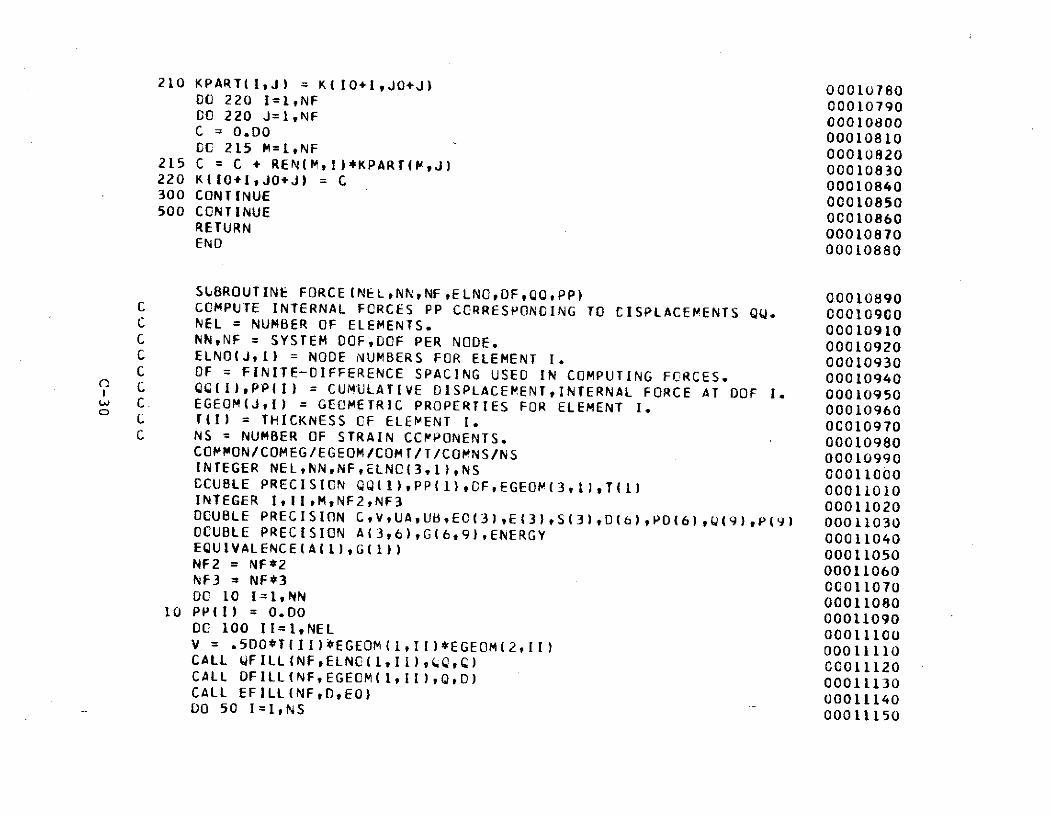
210 KPART(I,J) = K(1O+1,JO+J) 0001078000 220 I=1,NF 0001079000 220 J=1,NF 00010800C = O.DO 00010810CC 215 M=1,NF 00010820
215 C = C + REN(M,I)*KPART(P,J) 00010830220 K(IO+IJO+J) = C 00010840300 CONTINUE 00010850500 CONTINUE 00010860
RETURN 00010870END 00010880
SLBROUTINE FORCE(NELNN,NF,ELNO,DF,QQ,PP) 00010890C COMPUTE INTERNAL FORCES PP CORRESPONDING TO CISPLACEMENTS QW. 00010900C NEL = NUMBER OF ELEMENTS. 00010910C NNNF = SYSTEM DOFDOF PER NODE. 00010920C ELNO(Jl) = NODE NUMBERS FOR ELEMENT 1. 00010930C DF = FINITE-DIFFERENCE SPACING USED IN COMPUTING FORCES. 00010940C QQ(I)PP(I) = CUMULATIVE DISPLACEMENTINTERNAL FORCE AT DOF I. 00010950C. EGEOM(JlI) = GEOMETRIC PROPERTIES FOR ELEMENT I. 00010960C T(l) = THICKNESS OF ELEMENT I. 00010970C NS = NUMBER OF STRAIN CCMPONENTS. 00010980
COMMON/COMEG/EGEOM/COMT/T/COMNS/NS 00010990INTEGER NELNNNF#ELNO(3,1),NS 00011000OCUBLE PRECISION QQi1),PP(1),OF,EGEOM(3,1),T(1) 00011010INTEGER III,M,NF2,NF3 00011020DOUBLE PRECISION CV,UA,UB,EO(3),E(3),S(3),D(6),PD(6),Q(9),P(9) 00011030OCUBLE PRECISION A(3,6),G(6,9),ENERGY 00011040EQUIVALENCE(A(I1),G(1)) 00011050NF2 = NF*2
00011060NF3 = NF*3 00011070DO 10 I=I,NN 00011080
10 PP(I) = 0.DO 00011090DO 100 II=1,NEL 00011100V = .5DOT(II)*EGEOM(1,II)*EGEOM(2,II) 00011110CALL QFILL(NFpELNC(1,II),(Q,~ ) 00011120CALL DFILL(NF,EGEOM(1tII)Q,o) 00011130CALL EFILL(NF,DEO) 00011140DO 50 I=1,NS 00011150
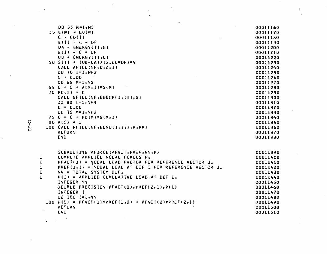
00 35 M=1,NS 0001116035 E(t) = EO(M) 00011170
C = EO(I) 00011180E(l) = C - OF 00011190UA = ENERGY(II,E) 00011200E(I) = C + OF 00011210UB = ENERGY(II,E) 00011220
50 S(I) = (UB-UA)/(2.O0*DF)*V 00011230CALL AFILL(NF,D,A,1) 0001124000 70 I=1,NF2 00011250C = 0.00DO 00011260DO 65 M=1,NS 00011270
65 C = C + A(MtI)*S(M) 0001128070 PD(I) = C 00011290
CALL GFILL(NFEGEOM(1,ll),G) 00011300DO 80 I=1,NF3 00011310C = 0.00DO 00011320DC 75 M=1,NF2 00011330
75 C = C + PD(M)*G(M,I) 0001134080 P(I) = C 00011350
100 CALL PFILL(NFELNO(1,II),P,PP) 00011360RETURN 00011370END 00011380
SUBROUTINE PFORCE(PFACT,PREF,NNP) 0001,1390C CCMPUTE APPLIED NODAL FCRCES P. 00011400C PFACT(J) = NODAL LOAD FACTOR FOR REFERENCE VECTOR J. 00011410C PREF(J,I) = NODAL LOAD AT DOF I FOR REFERENCE VECTOR J. 00011420C NN = TOTAL SYSTEM DOF. 00011430C P(I) = APPLIEDCUMULATIVE LOAD AT DOF I. 00011440
INTEGER NN 00011450DOUBLE PRECISION PFACT(IIPREF(2,1),P(1) 00011460INTEGER I 00011470CO ICO I=I,NN 00011480
100 P(I) = PFACT(1)*PREF(1,l) + PFACT(2) PREF(2,I) 00011490RETURN 00011500END 00011510
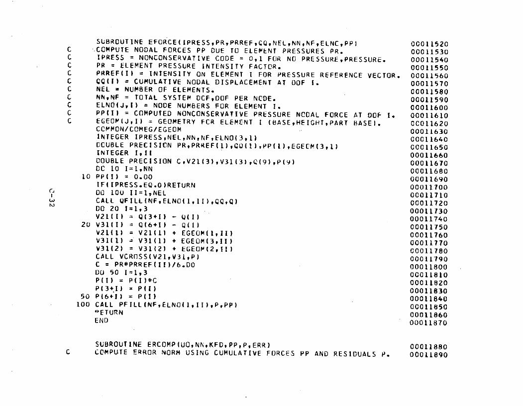
SUBROUTINE EFORCE(IPRESSPRtPRREF,CQ,NELNN,NF,ELNCPP) 00011520C -CCMPUTE NODAL FORCES PP DUE TO ELEMENT PRESSURES PR. 00011530C IPRESS = NONCONSERVATIVE CODE = 0,1 FOR NO PRESSURE,PRESSURE. 00011540C PR = ELEMENT PRESSURE INTENSITY FACTOR. 00011550C PRREF(I) = INTENSITY ON ELEMENT I FOR PRESSURE REFERENCE VECTOR. 00011560C CQMI) = CUMULATIVE NODAL DISPLACEMENT AT DOF 1. 00011570C NEL = NUMBER OF ELEMENTS. 00011580C NN,NF = TOTAL SYSTEM DCFDOF PER NCDE. 00011590C ELNO(JIl) = NODE NUMBERS FOR ELEMENT I. 00011600C PP(I) = COMPUTED NONCONSERVATIVE PRESSURE NCODAL FORCE AT DOF I. 00011610C EGEOM(JI) = GEOMETRY FCR ELEMENT I (BASEHEIGHT,PART HASE). 00C011620
CCMMON/COMEG/EG EOM 00011630INTEGER IPRESSNEL,NN,NFELNO(3t1) 00011640CCUBLE PRECISION PR,PRREF(1),QQ(),PP(1),EGECM(3,1) 00011650INTEGER 1,11 00011660DOUBLE PRECISION C,V21(3),V31(3),Q(9),P(9) 00011670DC 10 I=1,NN 00011680
10 PP(I) = O.DO 00011690IF(IPRESS.EQ.O)RETURN 00011700D 100O II=1,NEL
00011710CALL QFILL{NF,ELNO(1,II),QQQ) 00011720DO 20 1=1,3 00011730V21(1) = Q(3+I) - I(I) 00011740
20 V31(I) = Q(6+1) - Q(1) 00011750V21(1) = V21(1) + EGEOM(1,II) 00011760V3111) = V31(1) + EGEOM(3,II) 00011770V31(2) = V31(2) + EGEOM(2,II) 00011780CALL VCROSS(V21,V31,P) 00011790C = PR*PRREF(II)/6.DO 00011800DO 50 I=1,3 00011810P(I) = P(I)*C 00011820P(3+I) = P(I) 00011830
50 P(6+1) = P(I) 00011840100 CALL PFILL(NF,ELNO(ItlI),P,PP) 00011850
"ETURN 00011860END 00011870
SUBROUTINE ERCOMP(UONNKFD,PPtPERR) 00011880C CCMPU.TE ERROR NORM USING CUMULATIVE FORCES PP AND RESIDUALS P. 00011890
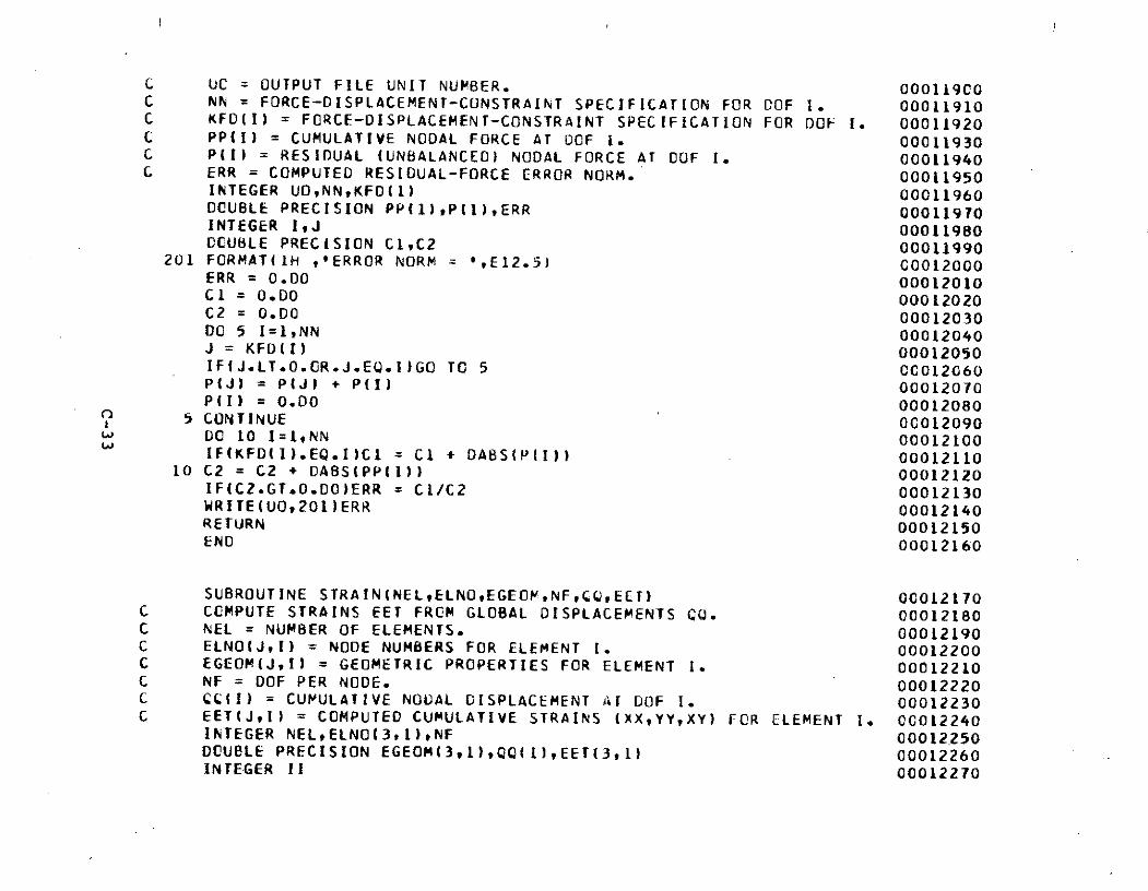
C UC = OUTPUT FILE UNIT NUMBER. 00011900C NN = FORCE-DISPLACEMENT-CONSTRAINT SPECIFICATION FOR 0OF I. 00011910C KFO(I) = FORCE-DISPLACEMENT-CONSTRAINT SPECIFICATION FOR DOF I. 00011920C PPI) = CUMULATIVE NODAL FORCE AT DOF 1. 00011930C P(I) = RESIDUAL (UNBALANCED) NODAL FORCE AT COF I. 00011940C ERR = COMPUTED RESIDUAL-FORCE ERROR NORM. 00011950
INTEGER UO,NNKFD(1) 00011960DOUBLE PRECISION PP(1),P(1),ERR 00011970INTEGER I,J 00011980DOCUBLE PRECISION C1,C2 00011990
201 FORMAT(IH ,'ERROR NORM = 1,E12.5) COO12000ERR = 0.00 00012010CI = 0.00 00012020C2 = 0.00 00012030DC 5 I=1,NN 00012040J = KFD(I) 00012050IF(J.LT.0.OR.J.EQ.I)GO TO 5 00012060P(J) = PIJ) + P(I) 00012070P(I) = 0.00 00012080
5 CONTINUE 00012090D0 10 I=1,NN 00012100IFIKFD(I).EQ.I)CI = Cl + DABS(P(1)) 00012110
10 C2 = C2 + DABS(PPII)) 00012120IF(C2.GT.0.DO)ERR = CI/C2 00012130WRITE(UO,201)ERR 00012140RETURN 00012150END 00012160
SUBROUTINE STRAIN(NELtELNOEGEOM,NFt~C,EET) 0C012170C COMPUTE STRAINS EET FROM GLOBAL DISPLACEMENTS QQ. 00012180C NEL = NUMBER OF ELEMENTS. 00012190C ELNO(JI) = NODE NUMBERS FOR ELEMENT 1. 00012200C EGEOM(JII) = GEOMETRIC PROPERTIES FOR ELEMENT 1. 00012210C NF = DOF PER NODE. 00012220C WI) = CUMULATIVE NODAL DISPLACEMENT AT DOF I. 00012230C EET(J,I) = COMPUTED CUMULATIVE STRAINS (XX,YY,XY) FOR ELEMENT 1. 00012240
INTEGER NEL,ELNO(3,t),NF 00012250DOUBLE PRECISION EGEOM(3,1),QQ(1),EET(3,1) 00012260INTEGER II 00012270
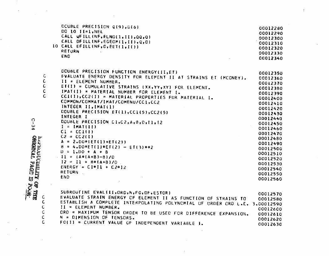
CCUBLE PRECISION Q(9),v(6) 0001228000 10 II=1,NEL 00012290CALL wFILL(NFELNO(1,II),QQtQ) 00012300CALL DFILLtNF,EGEOM(ltll),Q,D) 00012310
10 CALL EFILL(NFOEET(1,II)) 00012320RETURN 00012330END 00012340
DOUBLE PRECISION FUNCTION ENERGY(II,ET) 00012350C EVALUATE ENERGY DENSITY FOR ELEMENT II AT STRAINS ET (MCONEY). 00012360C II = ELEMENT NUMBER. 00012370C ET(I) = CUMULATIVE STRAINS (XX,YY,XY) FOR ELEMENT. 00012380C IAT(I) = MATERIAL NUMBER FOR ELEMENT I. 00012390C CCIII),CC2(I) = MATERIAL PROPERTIES FOR MATERIAL I. 00012400
COMMON/COMMAT/IMAT/COMENU/CCICC2 00012410INTEGER II,IMAT(I) 00012420DOUBLE PRECISION ET(.II),CCI(5),CC2(5) 00012430INTEGER I 00012440DOUBLE PRECISION C1,C2,A,18tDtI1I2 00012450I = IMAT(II) 00012460Cl = CCIII) 00012470C2 = CC2(1) 00012480A = 2.DO*(ET(1)+ET(2)) 00012490B = 4.DO*ET(1)*ET(2) - ET(3)**2 00012500D = 1.1)0 + A + B 0001251011 = (A*(A+B)-B)/O 0001252012 = II + 8*(A+B)/O 00012530ENERGY C1*I1 + C2*12 00012540RETURN 00012550END 00012560
C SUBROUTINE EVALIII,ORD,N,FO,DFESTOR) 00012570
C EVALUATE STRAIN ENERGY OF ELEMENT II AS FUNCTION OF STRAINS TO 00012580C ESTABLISH A COMPLETE INTERPOLATING POLYNOMIAL OF ORDER CRD L.E. 3.00012590C II = ELEMENT NUMBER. 00012600C ORD = MAXIMUM TENSOR ORDER TO BE USED FOR DIFFERENCE EXPANSION. 00012610C N = DIMENSION OF TENSORS. 00012620C FO(I) CURRENT VALUE CF INDEPENDENT VARIABLE 1. 00012630
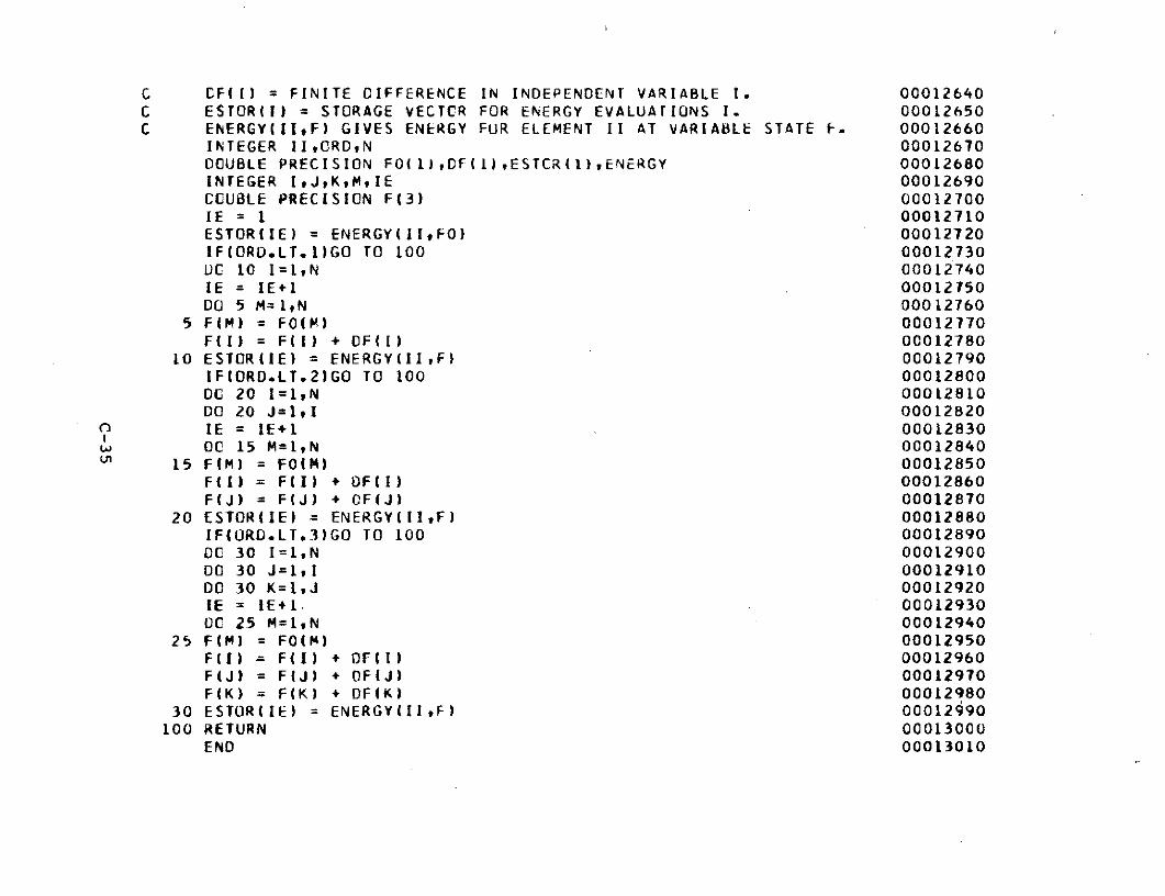
C CF(I) = FINITE DIFFERENCE IN INDEPENDENT VARIABLE 1. 00012640C ESTOR(I) = STORAGE VECTCR FOR ENERGY EVALUATIONS I. 00012650C ENERGY(II,F) GIVES ENERGY FUR ELEMENT II AT VARIABLE STATE F. 00012660
INTEGER II,ORD,N 00012670DOUBLE PRECISION FO(1),DF(1),ESTCR(I),ENERGY 00012680INTEGER I,JtK,M,IE 00012690CCUBLE PRECISION F(3) 00012700IE = 1 00012710ESTORIIE) = ENERGY(II,FO) 00012720IF(ORD.LT.1)GO TO 100 00012730UC 10 I=1,N 00012740IE = IE+1 0001275000 5 M=1,N 00012760
5 F(M) = FO(M) 00012770F(I) = F(I) + OF(1) 00012780
O1 ESTOR(IE) = ENERGY(II,F) 00012790IF(ORD.LT.2)GO TO 100 000128000D 20 I=1,N 00012810DO 20 J=1,Il 00012820IE = IE+1 0001283000 15 M=1,N 00012840
15 F(M) = FO(M) 00012850F(1) = F(I) + OF(I) 00012860F(J)(J) (J) + CF(J) 00012870
20 ESTOR(IE) = ENERGY(II,F) 00012880IF(ORD.LT.3)GO TO 100 00012890DC 30 I=1,N 0001290000 30 J=1,I 00012910DO 30 K=1,J 00012920IE = IE+1 00012930C00 25 M=1,N 00012940
25 F(M) = FO(M) 00012950F(I) = F(I) + OF(I) 00012960F(J) = F(J) + DF(J) 00012970F(K) = F(K) + DF(K) 00012980
30 ESTOR(IE) = ENERGY(IIF) 00012490100 RETURN 00013000
END 00013010
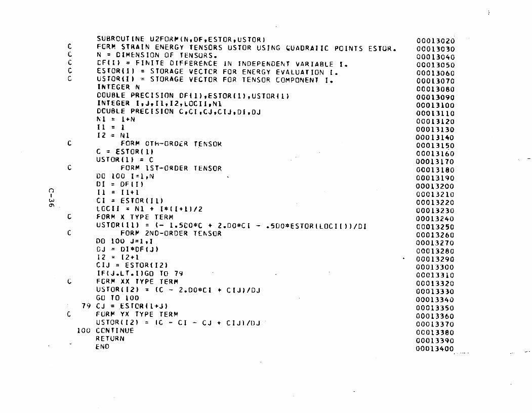
SUBROUTINE U2FORM(N,DFESTOR,USTOR) 00013020C FORM STRAIN ENERGY TENSORS USTOR USING QUADRAIIC POINTS ESTOR. 00013030C N = DIMENSION OF TENSORS. 00013040C CFII) = FINITE DIFFERENCE IN INDEPENDENT VARIABLE I. 00013050C ESTOR(I) = STORAGE VECTCR FOR ENERGY EVALUATION 1. 00013060C USTORII) = STORAGE VECTOR FOR TENSOR COMPONENT I. 00013070
INTEGER N 00013080DOUBLE PRECISION DF(1),ESTOR(1),USTOR(1) 00013090INTEGER ItJtIl1I2,LOCIINl 00013100DOUBLE PRECISION CCICJtCIJtDIDJ 00013110NI = 1+N 00013120II = 1 0001313012 = NI 00013140
C FORM OTH-ORDER TENSOR 00013150C = ESTOR(1) 00013160USTOR(1) = C 00013170
C FORM IST-ORDER TENSOR 0001318000 100 I=1,N 00013190DI = DF(I) 0001320011 = 11+1 00013210CI = ESTOR(I1) 00013220LOCII = N1 + I(1+1)/2 00013230
C FORM X TYPE TERM 00013240USTOR(11) = (- 1.5COC* + 2.00*CI - .500*ESTOR(LOCII))/DI 00013250
C FORM 2ND-ORDER TENSOR 00013260DO 100 J=1,I 00013270CJ = DI*DF(J) 0001328012 = 12+1 00013290CIJ = ESTOR(12) 00013300IF(J.LT.I)GO TO 79 00013310
C FORM XX TYPE TERM 00013320USTOR(12) = (C - 2.00DCI + CIJ)/DJ 00013330GO TO 100 00013340
79 CJ = .ESTOR(+J) 00013350C FORM YX TYPE TERM 00013360
USTOR(12) = (C - CI - CJ + CIJ)/I)J 00013370100 CCNTINUE 00013380
RETURN 00013390END 00013400
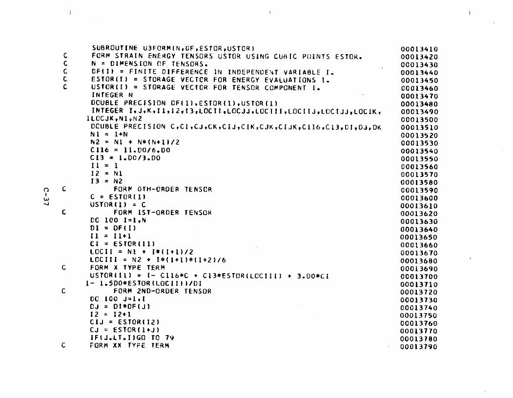
SUBROUTINE U3FORM(NUFESTOR*USTOR) 00013410C FORM STRAIN ENERGY TENSORS USTOR USING CUBIC POINTS ESTOR. 00013420C N = DIMENSION OF TENSORS. 00013430C DF(1) = FINITE DIFFERENCE IN INDEPENDENT VARIABLE 1. 00013440C. ESTOR(I) = STORAGE VECTOR FOR ENERGY EVALUATIONS 1. 00013450C USTORIl) = STORAGE VECTOR FOR TENSOR COMPONENT 1. 00013460
INTEGER N 0001.3470DOUBLE PRECISION OF(I),ESTOR(I),USTOR(1) 00013480INTEGER IJtKIIl,12,I3tLOCIILOCJJ,LOCIII,LOCIIJ,LCCIJJLOCIK, 00013490
1LOCJK,NlN2 00013500DCUBLE PRECISION CCI,CJ,CK,CIJCIKtCJKCICKIJKC116,C13, DJ,DK 00013510NI = 1+N 00013520N2 = Nl + N*(N+I)/2 00013530C116 = 11.00/6.00 00013540C13 = 1.DO/3.DO 00013550II = 1 0001356012 = Nl 0001357013 = N2 00013580
C FORM OTH-ORDER TENSOR 00013590C = ESTOR(1) 00013600USTOR(1) = C 00013610
C FORM 1ST-ORDER TENSOR 0001362000 100 I=1,N 00013630DI = DF(I) 0001364011 = 11+1 00013650CI = ESTOR(11) 00013660LOCII = Nl + I*(I+1)/2 00013670LOCIII = N2 + I(I+1)*(1+2)/6 00013680
C FORM X TYPE TERM 00013690USTORfII) = (- C116*C + C13*ESTOR(LOCIII) + 3.00*CI 000137001- 1.500OESTOR(LOCII))/DI 00013710
C FORM 2ND-ORDER TENSOR 00013720DG 100 J=1l, 00013730DJ = DI*DF(J) 0001374012 = 12+1 00013750CIJ = ESTOR(12) 00013760CJ = ESTORII(J) 00013770IF(J.LT.I)GO TO 79 00013780
C FORM XX TYPE TERM 00013790
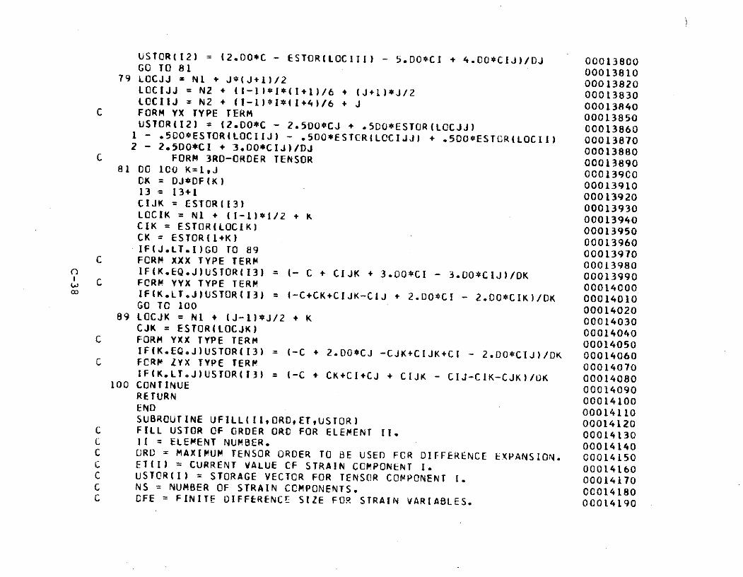
USTOR(12) = 42.DO*C - ESTOR(LOCIII) - 5.D0*CI + 4.00*CIJ)/DJ 00013800GO TO 81 00013810
79 LOCJJ = NI + J*(J+1)/2 00013820LOCIJJ = N2 + (I-1)*I*(I+1)/6 + (J+1)*J/2 00013830LOCIIJ = N2 + (I-1)*I*(I+4)/6 + J 00013840
C FORM YX TYPE TERM 00013850USTOR(12) = (2.DO* - 2.500*CJ + .500*ESTOR(LOCJJ) 00013860
1 - .5D0*ESTOR(LOCIIJ) - .500*ESTCR(LOCIJJ) + .500*ESTUR(LOCII) 000138702 - 2.5D0*CI + 3.00*CIJ)/DJ 00013880
C FORM 3RD-ORDER TENSOR 0001389081 00 100 K=1,J 00013900
OK = DJ*DF(K) 0001391013 = 13+1 00013920CIJK = ESTOR(13) 00013930LOCIK = NI + (1-1)*I/2 + K 00013940CIK = ESTORILOCIK) 00013950CK = ESTOR(1+K) 00013960IF(J.LT.I)GO TO 89 00013970
C FORM XXX TYPE TERM 00013980a IF(K.EQ.J)USTOR(13) = (- C + CIJK + 3.O0*CI - 3.00*CIJ)/DK 00013990
C FORM YYX TYPE TERM 000140000 IF(K.LT.J)USTOR(13) = (-C+CK+CIJK-CIJ + 2.DO*CI - 2.DO*CIK)/DK 00014010
GO TO 100 0001402089 LOCJK = Nl + (J-L)*J/2 + K 00014030
CJK = ESTOR(LOCJK) 00014040C FORM YXX TYPE TERM 00014050
[F(K.EQ.J)USTOR(13) = (-C + 2.DO*CJ -CJK+CIJK+CI - 2.DO*CIJ)/DK 00014060C FCRM LYX TYPE TERM 00014070
IF(K.LT.J)USTOR(13) = (-C + CK+CI+CJ + CIJK - CIJ-CIK-CJK)/DK 00014080100 CONTINUE 00014090
RETURN 00014100END 00014110SUBROUTINE UFILL(II,ORD,ETUSTOR) 00014120
C FILL USTOR OF ORDER ORD FOR ELEMENT II. 00014130C II = ELEMENT NUMBER. 00014140C ORD = MAXIMUM TENSOR ORDER TO BE USED FOR DIFFERENCE EXPANSION. 00014150C ET(1) = CURRENT VALUE CF STRAIN COMPONENT I. 00014160C USTCR(I) = STORAGE VECTOR FOR TENSOR COMPONENT 1. 00014170C NS = NUMBER OF STRAIN CCMPONENTS. 00014180C CFE FINITE DIFFERENCE SIZE FOR STRAIN VARIABLES. 00014190
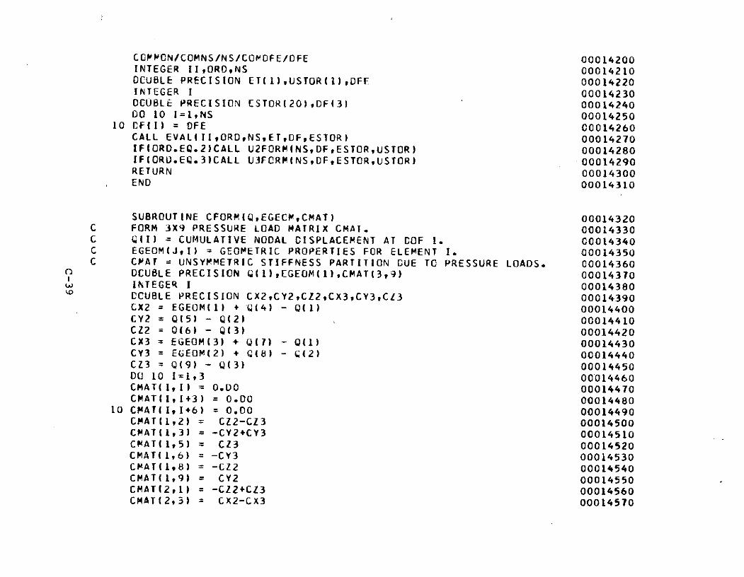
COMMCN/COMNS/NS/COMDFE/DFE 00014200INTEGER IIORD,NS 00014210DOCUBLE PRECISION ET(1),USTOR(1),DFF 00014220INTEGER 1 00014230DCUBLE PRECISION ESTOR(20),DF(3) 00014240DO 10 I=1,NS 00014250
10 CF(I) = DFE 00014260CALL EVAL(II,ORDNSET,DF,ESTOR) 00014270IF(ORD.EQ.2)CALL U2FORM(NS,DF,ESTOR,USTOR) 00014280IF(ORD.EQ.3)CALL U3FCRMINS,DF,ESTOR,USTOR) 00014290RETURN 00014300END 00014310
SUBROUTINE CFORMIQ,EGECM,CMAT) 00014320C FORM 3X9 PRESSURE LOAD MATRIX CMAT. 00014330C Q(I) = CUMULATIVE NODAL DISPLACEMENT AT COF 1. 00014340C EGEOM(JI) = GEOMETRIC PROPERTIES FOR ELEMENT I. 00014350C CMAT = UNSYMMETRIC STIFFNESS PARTITION DUE TO PRESSURE LOADS. 00014360
DOCUBLE PRECISION Qt1),EGEOM(1),CMAT(3,9) 00014370INTEGER I 00014380SCUBLE PRECISION CX2,CY2,CZ2,CX3,CY3,CZ3 00014390CX2 = EGEOM(I) + Q(4) - Q(1) 00014400CY2 = 0(5) - Q(2) 00014410CZ2 = 0(6) - Q(3) 00014420CX3 = EGEOM(3) + 017) - Q(1) 00014430CY3 = EGEOM(2) + Q(8) - C(2) 00014440CZ3 = Q(9) - Q(3) 00014450DO 10 I=1,3 00014460CMAT(I,I) = 0.00 00014470CMAT(II+3) = 0.00 00014480
10 CHAT(I,I+6) = 0.00 00014490CMAT(I,2) = C12-CZ3 00014500CMAT(1,3) = -CY2+CY3 00014510CMAT(1,5) = CZ3 00014520CMAT(1,6) = -CY3 00014530CMAT(1,8) = -CZ2 00014540CMAT(1,9) = CY2 00014550CMAT(2,1) = -CZ2+CZ3 00014560CMAT(2,3) = CX2-Cx3 00014570
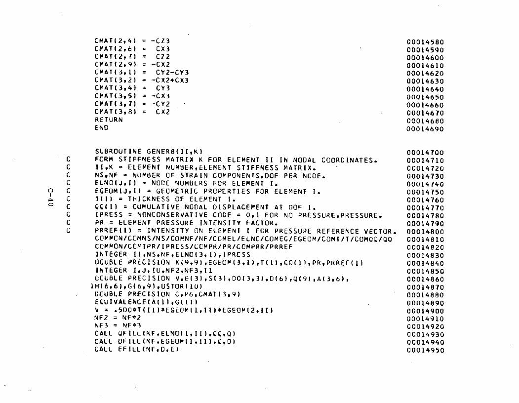
CMAT(2,4) = -CZ3 00014580CMAT(2,6) = CX3 00014590CMAT(217) = CZ2 00014600CMATI29) = -CX2 00014610CMAT(3 1) = CY2-CY3 00014620CMAT(3,2) = -CX2+CX3 00014630CMAT(394) = CY3 00014640CMAT(3,5) = -CX3 00014650CMAT(3,7) = -CY2 00014660CMAT(3,8) = CX2 00014670RETURN 00014680END 00014690
SUBROUTINE GENER8(II,K) 00014700C FORM STIFFNESS MATRIX K FOR ELEMENT II IN NODAL CCORDINATES. 00014710C II,K = ELEMENT NUMBER,ELEMENT STIFFNESS MATRIX. 00014720C NSNF = NUMBER OF STRAIN COPPONENTS,DOF PER NCODE. 00014730C ELNO(J,I) = NODE NUMBERS FOR ELEMENT I. 00014740C EGEOMJIl) = GEOMETRIC PROPERTIES FOR ELEMENT I. 00014750C T(I) = THICKNESS OF ELEMENT 1. 00014760C CQII) = CUMULATIVE NODAL DISPLACEMENT AT DOF I. 00014770C IPRESS = NONCONSERVATIVE CODE = 0,1 FOR NO PRESSURE,PRESSURE. 00014780C PR = ELEMENT PRESSURE INTENSITY FACTOR. 00014790L PRREF(I) = INTENSITY ON ELEMENT I FOR PRESSURE REFERENCE VECTOR. 00014800
COMMCN/COMNS/NS/COMNF/NF/COMEL/ELNC/COMEG/EGEOM/COMT/T/COMQQ/QQ 00014810COMMON/COMIPR/IPRESS/CCMPR/PR/CCMPRR/PRREF 00014820INTEGER II,NS,NF,ELNO(31),IPRESS 00014830DOUBLE PRECISION K(9,9),EGEOM(31),T(1),CQ(1),PR,PRREF(1) 00014840INTEGER I,J,IU,NF2,NF3,I1 00014850CCUBLE PRECISION V,E(3),S(3),00(393),D(6),Q(9),At3,6)t 00014860IH(6,6),G(6,9),USTOR(1O) 00014870OCUBLE PRECISION C,P6,CMAT(3,9) 00014880ECUIVALENCEtA(1),G(1)) 00014890V = .5SD0T(II)*EGEOM(1,II)*EGEOP(2,II) 00014900NF2 = NF*2 00014910NF3 = NF*3 00014920CALL QFILLINF,ELNO( 1,I),QQ,Q) 00014930CALL OFILL(NF,EGEOMIl,il),Q,D) 00014940CALL EFILL(NF,D,E) 00014950
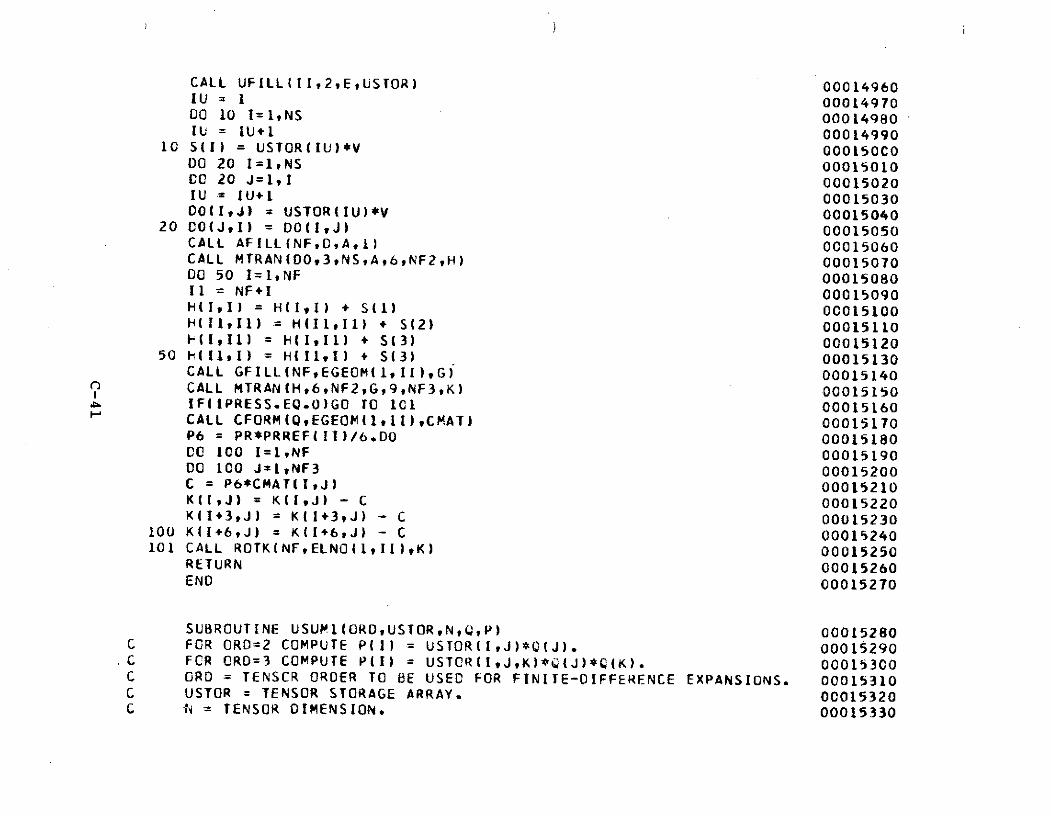
CALL UFILL(II,2,E,USTOR) 00014960IU = 1 00014970DO 10 I=1,NS 00014980IU = IU+1 00014990
10 S(1) = USTOR(IU)*V 000150CDO 20 I=1,NS 00015010CO 20 J=1,I 00015020IU = IU+1 0001503000(1,J) = USTOR(IU)*V 00015040
20 00(JtI) = DO(I1J) 00015050CALL AFILL(NF,0,A,1) 00015060CALL MTRAN(DO,3,NSA,6,NF2tH) 00015070DO 50 1=1,NF 0001508011 = NF+I 00015090H(ItI) = H(I1I) + S(1) 00015100H(IlI1) H(I11,Ill + S(2) 00015110-(1,11) = H(IIl) + S(3) 00015120
50 H(1,1) = H(ll,I) + S(3) 00015130CALL GFILL(NF,EGEOM(I1,1),G) 00015140CALL MTRAN(H,6,NF2,G,9,NF3,K) 00015150IF(IPRESS.EQ.0)GO TO 101 00015160CALL CFORM(QEGEOM(llII),CMAT) 00015170P6 = PR*PRREF(II)/6.DO 00015180CC 100 I=,NF 00015190DO 100 J=i,NF3 00015200C = P6*CMAT(TI,J) 00015210K(I,J) = K(I,J) - C 00015220K(I+3,J) = K(I+3,J) - C 00015230
100 K(I+6,J) = K(I+6,J) - C 00015240101 CALL ROTK(NF,ELNO41,Il),K) 00015250
RETURN 00015260END 00015270
SUBROUTINE USUML(ORD,USTOR,NQ,P) 00015280C FOR ORD=2 COMPUTE P(1) = USTOR(I,J)*Q(J). 00015290
.C FOR ORD=3 COMPUTE P(I) = USTOR(IJK)*Q(J)*Q(K). 00015300C ORD = TENSCR ORDER TO BE USED FOR FINITE-DIFFERENCE EXPANSIONS. 00015310C USTOR = TENSOR STORAGE ARRAY. 00015320C T = TENSOR DIMENSION. 00015330
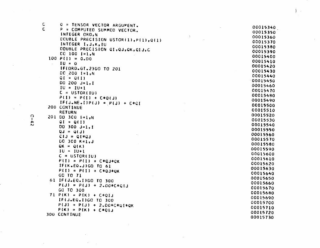
C 0 = TENSOR VECTOR ARGUPENT. 00015340C P = COMPUTED SUMMED VECTOR. 00015350
INTEGER ORD,N 00015360OCUBLE PRECISION USTOR(1),P(1),Q(1) 00015370INTEGER I,J,K,IU 00015380DOUBLE PRECISION QIQJQK,QIJ,C 00015390CC 100 I=I,N 00015400
100 P(I) = O.DO 00015410IU = 0 00015410
IF(ORO.GT.2)GO TO 201 00015430DO 200 I=1,N 00015440QI = Q(1) 00015440
00 200 J=1,I 00015460IU IU+I 00015470C = USTOR(IU) 00015470P(I) = P(I) + C*Q(J) 0001540IF(J.NE.I)P(J) = P(J) + I 00015490
200 CONTINUE 00015500RETURN 00015510
201 00 300 l=1N 00015520QI = Q(I) 00015530
DO 300 J=1,I 00015540QJ = Q(J) 00015550IJ = QI*Qj 00015560
00 300 K=,J 00015570QK =Q(K) 00015580
IU = IU+1 00015590
C = USTOR(IU) 00015610Pi) = P(l) + C*QJ*CK 00015610
IF(K.EQ.J)GO TO 61 00015630P(l) = P(I) + C*QJ*QK 00015640GO TO 71 00015640
61 IFIJ.EQ.I)GO TO 300 00015660P(J) = P(J) + 2.O0*C*QIJ 00015670GO TO 300
0001568071 P(K) = P(K) + C*QIJ 00015690IF(J.EQ.I)GO TO 300 00015700P(J) = PlJ) + 2.00*C*I0*QK 00015710P(K) = P(K) + C*QIJ
300 CONTINUE 0001572000015730
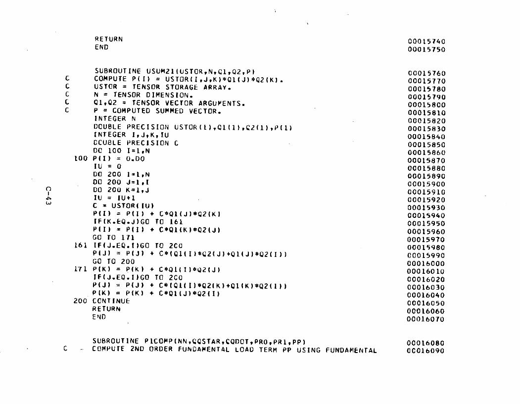
RETURN 00015740END 00015750
SUBROUTINE USUM21(USTOR,N,Q,Q2, P) C0015760C COMPUTE P(I) = USTOR(I,J,K)*Q1(J)*Q2(K). 00015770C USTOR = TENSOR STORAGE ARRAY. 00015780C N = TENSOR DIMENSION. 00015790C 01,Q2 = TENSOR VECTOR ARGUMENTS. 00015800C P = COMPUTED SUMMED VECTOR. 00015810
INTEGER N 00015820DOUBLE PRECISION USTOR(1),Q1(1) ,2(1),P(1) 00015830INTEGER IJK,IU 00015840CCUBLE PRECISION C 00015850DO 100 I=1,N 00015860
100 P(I) = O.DO 00015870IU = 0 00015880DO 200 I=1,N 00015890DO 200 J=1,I 00015900DO 200 K=1,J 00015910IU = IU+1 00015920C = USTOR(IU) 00015930P(I) = P(I) + C*QI(J)*Q2(K) 00015940IF(K.EQ.J)GO TO 161 00015950P(I) = P(I) + C*Q1(K)*Q2(J) 00015960GO TO 171 00015970
161 IFIJ.EQ.I)GO TO 2C00 00015980P(J) = P(J) + C*(Q1(I)*C2(J)+Q1(J)*Q2(I)) 00015990GO TO 200 00016000
171 P(K) = P(K) + C*Q1(1)*Q2(J) 00016010IF(J.EQ.I)GO TO 2C0 00016020P(J) P(J) + C*(Q(I)*Q2(K)+QI(K)*Q2(I)) 00016030P(K) = P(K) + C*Q1(J)*Q2(1) 00016040
200 CONTINUE 00016050RETURN 00016060END 00016070
SUBROUTINE PICOMP(NN,QCSTARCQDOTPRO,PR1,PP) 00016080C - COMPUTE 2ND ORDER FUNDAMENTAL LOAD TERM PP USING FUNDAMENTAL 00C016090
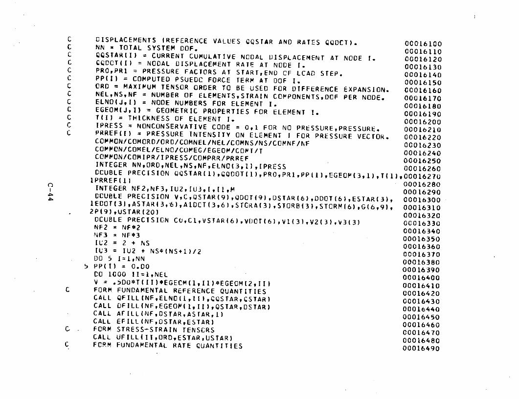
C DISPLACEMENTS (REFERENCE VALUES QQSTAR AND RATES CODCT). 00016100C NN = TOTAL SYSTEM DOF. 00016110C CQSTAR(I) = CURRENT CUMULATIVE NCODAL DISPLACEMENT AT NODE 1. 00016120C CCCTII) NODAL DISPLACEMENT RATE AT NODE 1. 00016130C PRO,PR1 PRESSURE FACTORS AT START,END CF LCAD STEP. 00016140C PP(I) = COMPUTED PSUEDO FORCE TERM AT DOF I. 00016150C ORD = MAXIMUM TENSOR ORDER TO BE USED FOR DIFFERENCE EXPANSION. 00016160C NEL,NS,NF = NUMBER OF ELEMENTSSTRAIN CCPPONENTS,0CF PER NODE. 00016170C ELNOiJI) = NODE NUMBERS FOR ELEMENT I. 00016180C EGEOM(JI) = GEOMETRIC PROPERTIES FOR ELEMENT 1. 00016190C T(I) = THICKNESS OF ELEMENT I. 00016200C IPRESS = NONCONSERVATIVE CODE = 0,1 FOR NO PRESSURE,PRESSURE. 00016210C PRREF(I) = PRESSURE INTENSITY ON ELEMENT I FOR PRESSURE VECTOR. 00016220
COMMON/COMCRD/ORC/COMNEL/NEL/COMNS/NS/COMNF/NF 00016230
COMMON/COMEL/ELNO/COMEG/EGEOM/COMT/T 00016240
COPPON/COMIPR/IPRESS/COMPRR/PRREF 00016250INTEGER NNORO,NEL,NS,NFELNO(3,1),IPRESS
00016260DOCUBLE PRECISION QQSTAR(l),QQDOT(1),PRO,PR1,PP(1),EGEOM(3,1),T(1),000162701PRREF(1)
00016280INTEGER NF2,NF3,IU2IU3,I1,II,M 00016290CCUBLE PRECISION VC,QSTAR(9),QDOT(9),DSTAR(6),DDOT(6),ESTAR(
3 ), 00016300IECOT( 3 ),ASTAR(3,'6),AIDCT(3,6),STCRA(3),STORB(3),STCRM(6 ),G(6,9), 00016310
2P(9),USTAR(20) 00016320OCUBLE PRECISION CO,C1,VSTAR(6),VI)OT(6),V1(3),V2(3),V3(3) 00016330
NF2 = NF*2 00016340
NF3 = NF*3 00016350
IU2 = 2 + NS 00016360IU3 = IU2 + NS*(NS+1)/2 00016370DO 5 I=1,NN 00016380
5 PP(I) = 0.00 00016390CO 1000 II=1,NEL 00016400V = .5DO*T(II)*EGECM(1,II)*EGEOM(2,11)
00016410C FORM FUNDAMENTAL REFERENCE QUANTITIES 00016420
CALL QFILL(NF,ELNC(1,[I),CSTAR,CSTAR) 00016430CALL OFILL(NF,EGEOP( 1IIll),QSTAR,DSTAR) 00016440CALL AFILL(NF,DSTAR,ASTAR,1) 00016450CALL EFILL(NFDSTARESTAR) 00016460
C. - FORM STRESS-STRAIN TENSCRS 00016470CALL UFILLIII,ORD,ESTAR,USTAR) 00016480
C FORM FUNDAMENTAL RATE QUANTITIES 00016490
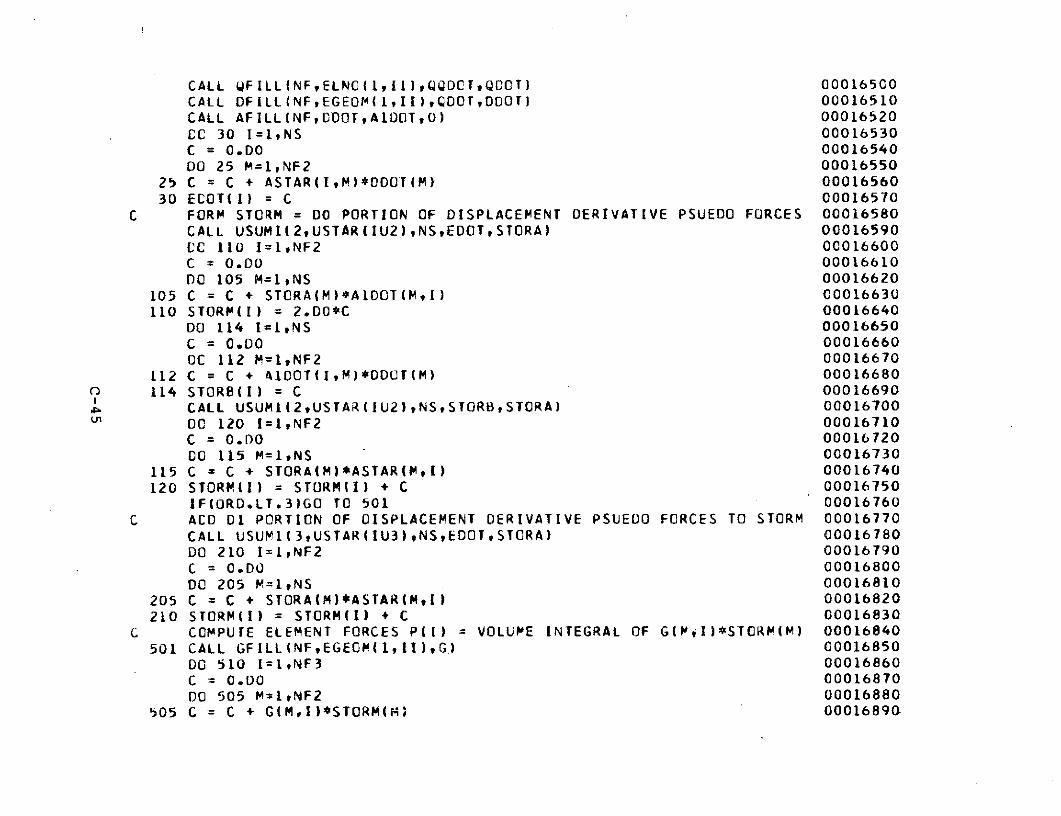
CALL QFILL(NF,ELNO(1,II),QQDCT,QDCT) 00016500CALL DFILL(NF,EGEOM(1,II),QDOT,DDOT) 00016510CALL AFILL(NF,CDOT,AIDOT,0) 00016520
CC 30 I=1,NS 00016530C = 0.00 00016540DO 25 M=1,NF2 00016550
25 C = C + ASTAR(1,M)*DDOT(M) 0001656030 ECOT(I) = C 00016570
C FORM STORM = DO PORTION OF DISPLACEMENT DERIVATIVE PSUEDO FORCES 00016580
CALL USUM1(2tUSTAR(IU2),NSEDOT,STORA) 00016590
CC 110 I=1,NF2 00016600C = 0.00 00016610
DO 105 M=1,NS 00016620
105 C = C + STORA(M)*AIDOT(M,I) 00016630110 STORM(I) = 2.DO*C 00016640
DO 114 I=1,NS 00016650
C = 0.00DO 00016660
OC 112 M=1,NF2 00016670
112 C = C + A100T(I,M)*DDOT(M) 00016680
114 STORB(I) = C 00016690
CALL USUMI(2,USTAR(IU2),NSSTORBSTORA) 00016700DC 120 I=1,NF2 00016710C = O.DO 0001672000 115 M=1,NS 00016730
115 C = C + STORA(M)*ASTAR(MI) 00016740
120 STORM(I) = STORM(l) + C 00016750IF(ORD.LT.3)GO TO 501 00016760
C ACD 01 PORTION OF DISPLACEMENT DERIVATIVE PSUEDO FORCES TO STORM 00016770
CALL USUM1( 3,USTAR(IU3),NSEDOT,STORA) 00016780
DO 210 I=1,NF2 00016790
C = 0.00DO 00016800DC 205 M=1,NS 00016810
205 C = C + STORA(M)*ASTAR(M,I) 00016820
210 STORM{I) = STORM(I) + C 00016830
C COMPUTE ELEMENT FORCES P(1) = VOLUME INTEGRAL OF G(MI)*STORM(M) 00016840
501 CALL GFILL(NF,EGEOM(1,11),G) 00016850
DO 510 I=1,NF3 00016860
C = 0.00 00016870
00 505 M=1,NF2 00016880505 C = C + G(MI)STORM(M) 00016890
510 P(I) = C*V 00016900IF(IPRESS.EQ.O)GO TO 1CCO 00016910
C ACD NONCONSERVATIVE PRESSURE FORCES TO P 00016920VSTAR(1) = EGEOM(1,II) + QSTAR(4) - QSTAR(1) 00016930VSTAR(2) = QSTAR(5) -. CSTAR(2) 00016940VSTAR(3) = QSTAR(6) - CSTAR(3) 00016950VSTAR(4) = EGEOM(3,II) + QSTAR(7) - CSTAR(1) 00016960VSTAR(5) = EGEOM(2,11) + QSTAR8) - QSTAR(2) 00016970VSTAR(6) = QSTAR(9) - QSTAR(3) 00016980VOTI(1) = 000T(4) - ODOT(1) 00016990VCOT(2) = Q0OT(5) - QCCT(2) 00017000VCOT(3) = QDOT(6) -. Q CT(3) 00017010VDOT(4) = QDOT(7) - ODCT(1) 00017020VCOT(5) = QDOT(8) - QCCT(2) 00017030VCOT(6) = 000T(9) - QDCT(3) 00017040CO = PRO*PRREF(II)/3.DO 00017050Cl = (PRI-PRO)*PRREF(II)/3.00 00017060CALL VCROSS(VDOT,VSTAR(4),V1) 00017070CALL VCROSS(VSTARVDOT(4),V2) 00017080CALL VCROSS(VDOT,VoOT(4),V3) 00017090CO 610 I=1,3 00017100C = C *(V1(I)+V2(I)) + CO*V3(I) 00017110P(1) = P(I) - C 00017120P(I+3) = P(I+3) - C 00017130610 P(I+6) = P(I+6) - C 00017140
C ACD ELEMENT FORCES P TO SYSTEM FORCES PP 000171501000 CALL PFILL(NFELNC(1,II),P,PP) 00017160RETURN 00017170END)
00017180
SUBROUTINE RATES(KMAT,PINN,KFD,RP,PRO,PRI,LSIGN,RLRRLRQ,RRQ) 00017190
C COMPUTE 1ST AND 2ND PATH RATES FOR LOAD DIRECTION VECTOR RP. 00017200C LCAD PARAMETER RATES = RL,RRL. DISPLACEMENT RATES = RQ,RRQ. 00017210C KMAT = SYSTEM JACOBIAN STIFFNESS MATRIX. 00011220C Pl = TEMPORARY FORCE STORAGE VECTOR. 00011230C NN = TOTAL SYSTEM DOF. 00011240C KFD(I) = FORCE-DISPLACEMENT-CONSTRAINT SPECIFICATION FCR DOF I. 0C017250C RP(1) = RESICUAL LOAD (LOAD STEP) AT DOF 1. 00017260C PRO,PRI = PRESSURE FACTORS AT START,END OF LOAD STEP. 00017270
C LSIGN = +,- IF LOAD PARAMETER IS INCREASING,CECREASING. 00017280C RL,RRL = COMPUTED LOAD PARAMETER IST,2ND ORDER RATES. 00017290C RQ(1),RRQ(I) = COMPUTED IST,2ND ORDER DISPLACEMENT RATE AT DOF I. 00017300C CC(I) = CURRENT CUMULATIVE DISPLACEMENT AT DCF I. 00C017310
COPPON/COMQQ/QQ 00017320INTEGER NNKFD(1) 00017330DOUBLE PRECISION RP(1),PROPR1,LSIGNRLRLRQ(I),RRQ(I)tQQ(1), 00017340IKMAT(NNNNbtP1(1) 00017350INTEGER I 00017360DOUBLE PRECISION RSIGN 00017370CALL SOLVE(KMATNNKFCRPRQ) 00017380CALL PICOMP(NN,QQRQ,PRO,PRI,P1) 00017390RL = 0.DO 00017400RRL = 0.00 00017410D00 50 I=1,NN 00017420IFIKFD(I).LT.0)GO TO 49 00017430.RL = RL + RP(I)*RQ(I) 00017440RRL = RRL + Pl(I)*RQ(I) 00017450GO TO 50 00017460
49 PlII) = 0.00 0001747050 CONTINUE 00017480
CALL SOLVE(KMATNNKFD,P,RRQ) 00017490DO 55 I=1,NN 00017500IF(KFD(I).GT.0)RRL = RRL + RP(I)*RRQ(I) 00017510
55 CONTINUE 00017520RSIGN = 1.00 00017530IF(RL.LT.0.O0)RSIGN = -1.00 00017540RL = RSIGN/RL 00017550RRL = RSIGN*RL**2*RRL*.500 00017560DO 60 I=1,NN 00017570
60 RRQ(I) = RRL*RQ(I) - RL*RRQ(I) 00017580RL = LSIGN*DSQRT(RL) 00017590DO 80 I=1,NN 00017600
80 RC(I) = RL*RQ(I) 00017610RETURN 00017620END 00017630
SUBROUTINE STEP(LSIGNRLRRL,NNRQ*RRQJUMPRMJUMPtNJUMPtDSLOPE, 00017640IPATHLAMS) 00017650
C COMPUTE PATH = PATH DISTANCE, LAMS = LOAD STEP SIZE. 00017660C LSIGN = +,- IF LOAD PARAMETER IS INCREASINGCECREASING. 00017670C RLPRRL = 1ST,2ND CRDER LOAD PARAMETER RATES. 00017680C NN = TOTAL SYSTEM DOF. 00017690C RQ(I),RRQ(I) = IST,2ND ORDER DIAPLACEMENT RATES AT DCF I. 00017700C JUMPR = FRACTION OF LOAD INCREMENT PRECEEDING LIMIT POINT 00017710C AT WHICH LIMIT IS TO BE TRAVERSED* 00017720C MJUMP = MAXIMUM NUMBER CF INCREMENT DIVISIONS TO PERFORM WHEN 00017730C NEARING A LIMIT POINT. 00011740C NJUMP = CURRENT NUMBER CF INCREMENT DIVISIONS TO PERFORM WHEN 00017750C NEARING A LIMIT POINT. 00017760C OSLOPE = MAXIMUM SLOPE RATIO (CHANGE/AVERAGE) DURING LOAD STEP. 00017770C PATH = COMPUTED PATH STEP SIZE TO BE TAKEN. 00017780C LAMS = INPUT MAXIMUM,CCMPUTED ACTUAL LOAD STEP SIZE. 00017790
INTEGER NN*MJUPP,NJUMP 00017800CCUBLE PRECISION LSIGN,RLtRRLtRQ(1),RRQ(1),JUMPRDSLOPEtPATHtLAMS 00017810INTEGER N,I 00017820DOUBLE PRECISION SLIM,LAMLIMtPREC,DSLOP,CRCRR,C C0017830IF(LSIGN*RL.LE.0.00)STOP 601 00017840IF(RL*RRL.GE.0.D0)O0 TO 21 00017850
C POSSIBLE LIMIT POINT 00017860SLIM = -RL/RRL 00017870
LAMLIM = DABS(SLIM*RL + .5SD0SLIM**2*kRL) 00017880C CHECK CLOSENESS OF LIMIT POINT 00017890
IF(LAMLIM.LT.JUMPR)GO TO 11 00017900IF(LAMS.LT.LAMLIM/MJUMP)GO TO 21 00017910
C LIMIT IS CLOSE. TAKE FRACTIONAL STEP JUMP 00011920NJUMP = NJUMP-1 00017930IF(NJUMP.LT.2)NJUMP = 2 00017940IF(LAMS.LT.LAMLIM)GO TO 7 00017950
C STEP IS LARGER THAN LIMIT. JUMP TOWARD LIMIT VALUE. 00017960LAMS = LAMLIM/NJUMP 00017970GO TO 10 00017980
C STEP IS SMALLER THAN LIMIT. JUMP TCWARD STEP VALUE. 000179907 N = NJUMP*LAMS/LAMLIM + 1 00018000
IF(N.EQ.I)NJUMP = NJUMP+1 00018010LAMS = LAMS/N 00018020
10 LAMS = LSIGN*LAMS C0018030PATH = (-RL+LSIGN*DSQRT(RL**2+2.00*LAMS*RRL))/RRL 00018040RETURN 00018050
C LIMIT IS VERY CLOSE. TRAVERSE THE LIMIT POINT 0001806011 NJUPP = MJUMP+1 00018070
LSIGN = -LSIGN 00018080LAMS = 0.DO 00018090PATH = -2.DO*RL/RRL 00018100RETURN 00018110
C LIMIT IS NOT CLOSE. CHECK SLOPE CHANGE FOR ALLOWABLE STEP 0001812021 NJUMP = MJUMP+1 00018130
CR = 0.00 00018140CRR = 0.00 00018150CC 50 I=1,NN 00018160CR = CR + DABS(RQ(II) 00018170
50 CRR = CRR + DABS(RRQ(I)) 00018180LAMS = LSIGN*LAMS 00018190
51 PREC = DABS(2.00*LAMS*RRL/RL**2) 00018200IF(PREC.LT.1.D-8)PATH = LAMS/RL 00018210IF(PREC.GE..D-8)PATH = (-RL+LSIGN*CSQRT(RL**2+2.00*LAMS*RRL))/RRL00018220OSLOP = PATH*RRL 00018230OSLOP = DSLOP/(RL+.5D00CSLOP) 00018240C = PATH*CRR 00018250C = C/(CR+.5DO*C) 00018260IF(DABS(CSLOP).LE.DSLOPE.ANC.C.LE.DSLOPE)RETURN 00018270LAMS = .5CO*LAMS 00018280IF(DABS(LAMS).LE.1.D-3)STOP 602 00018290GC TO 51 00018300END 00018310
SUBROUTINE EIGENI(NN,NCODE,QQDELTSCRITCGPOST,LAMPROPRI,Pp) 00018320C FORM POSTBUCKLING LOAD TERM PP USING FUNDAMENTAL DISPLACEMENTS 00018330C (REFERENCE VALUES CQSTAR AND CRITICAL INCREMENT QQDELT) AND 00C018340C POSTBUCKLING DISPLACEMENT EIGENVECTOR ~CPOST. 00018350C NN = TOTAL SYSTEM DOF. 00018360C NCODE = 0,1 FOR LINEAK,NONLINEAR EIGEN SOLUTION. 00018370C CQDELT(I) = ESTIMATED INCR. DISPLACEMENT AT CUF I TO CRITICAL PT. 00018380C SCRIT = ESTIMATED INCREMENTAL PATH VALUE TO CRITICAL PCINT. 00018390C QQPOST(I) = ESTIMATED BUCKLING DISPLACEMENT AT DOF I. 0C018400C LAM = ESTIMATED INCREMENTAL LOAD PARAMETER VALUE TO CRITICAL PT. 00018410C PR0,PRI = PRESSURE FACTORS AT STARTEND GF LCAD STEP. 00018420C PP(I) = COMPUTED RIGHT-HAND-SIDE FCR INVERSE POWER ITERATION. 00018430
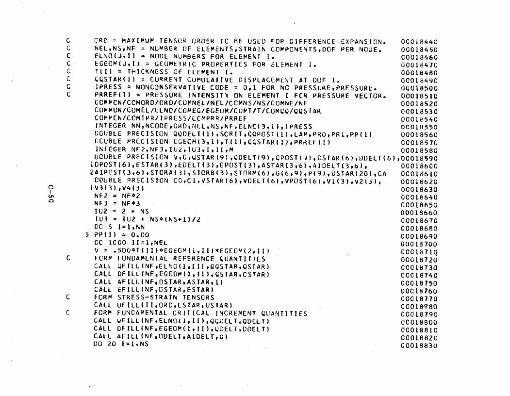
C ORC = MAXIMUM TENSOR ORDER TC BE USED FOR DIFFERENCE EXPANSION. 00018440C NEL,NSNF = NUMBER OF ELEMENTSSTRAIN COMPONENTS,DOF PER NODE. 00018450C ELNOIJ,I) = NODE NUMBERS FOR ELEMENT I. 00018460C EGEOM(J,I) = GEOMETRIC PROPERTIES FOR ELEMENT I. 00018470C T(I) = THICKNESS OF ELEMENT 1. 00018480C CCSTAR(I) = CURRENT CUMULATIVE DISPLACEMENT AT DOF I. 00018490C IPRESS = NONCONSERVATIVE CODE = 0,1 FOR NC PRESSURE,PRESSURE. 00018500C PRREF(I) = PRESSURE INTENSITY ON ELEMENT I FCR PRESSURE VECTOR. 00018510
CCPPCN/COMORD/ORD/COMNEL/NEL/COMNS/NS/COMNF/NF 00018520COMMON/COMEL/ELNO/COMEG/EGEOM/COMT/T/COMQQ/QQSTAR 00018530CONMCN/CCMIPR/IPRESS/CCMPRR/PRREF 00018540INTEGER NNNCODE,ORDNEL,NS,NFELNC(3,1),1PRESS 00018550COUBLE PRECISION QQDELT(l),SCRIT,CQPOST(1),LAMPRO,PR1,PP(1) 00018560ECUBLE PRECISION EGECM(3,1),T(1),CQSTAR(1),PRREF(1) 00018570INTEGER NF2,NF3,U2,IU3,I,II,M 00018580DCUBLE PRECISION V,C,tSTAR(9),QDELT(9),CPOST(9),DSTAR(6),DDELT(6),O0018590IDPOST(6),ESTAR(3)EDELT(3),EPOST(3),ASTAR(3,6),AIDELT(3,b), 000186002APOSTI(3,6),STORA(3),STCRB(3),STORM(6),G(6,9),P(9),USTAR(20),CA 00018610DCUBLE PRECISION C0,C1,VSTAR(6),VOELT(6),VPOST(6),VI(3),V2(3), 00018620
1V3(3),V4(3) 00018630i NF2 = NF*2 00018640
0 NF3 = NF*3 00018650IU2 = 2 + NS 00018660IU3 = IU2 + NS*(NS+I)/2 00018670DC 5 I=1,NN 00018680
5 PP(I) = 0.00 00018690CC 100C0 II=1,NEL 00018700V = .500*T(II)*EGECM(1,II)*EGEOM(2,11) 00018710
C FORM FUNDAMENTAL REFERENCE QUANTITIES 00018720CALL QFILL(NF,ELNG(1,II),QQSTAR,QSTAR) 00018730CALL DFILL(NF,EGEOM(1,II),QSTARCSTAR) 00018740CALL AFILL(NF9DSTAR,ASIAR,1) 00018750CALL EFILL(NFUDSTAR,ESTAR) 00018760
C FORM STRESS-STRAIN TENSORS 00018770CALL UFILL(IIORD,ESTAR,USTAR) 00018180
C FORM FUNDAMENTAL CRITICAL INCREMENT QUANTITIES 00018790CALL FILL(NF,ELNC(LII),QDELT,QDELT) 00018800CALL OFILL(NFEGEOM(1,Il),QDELT,DDELT) 00018810CALL AFILL(NF,DDELT,AIDELT,0) 00018820DO 20 I=1,NS 00018830
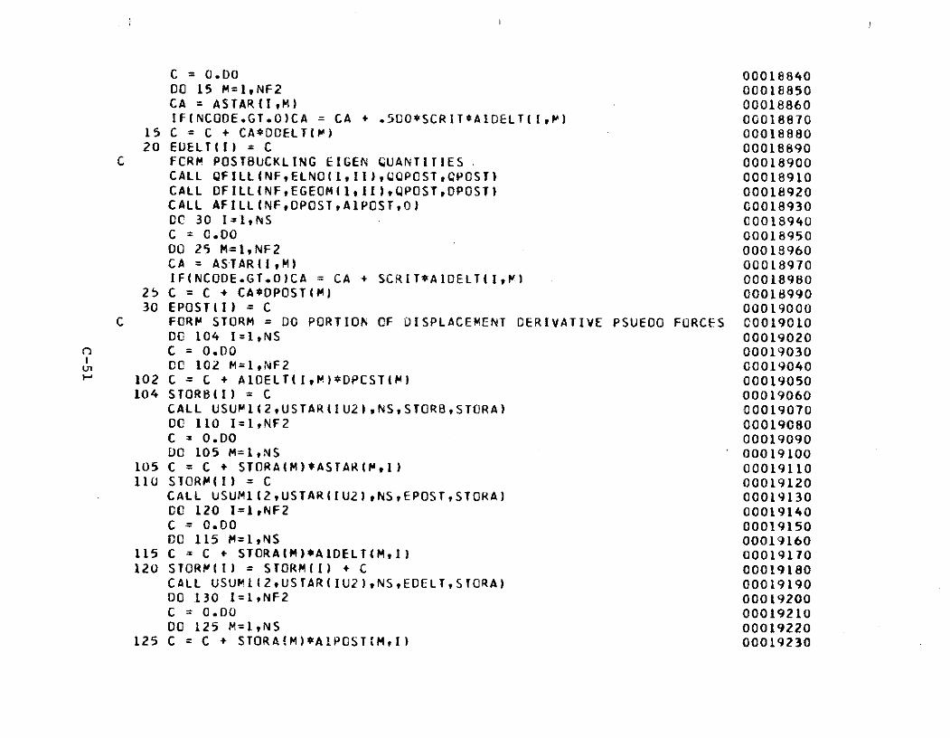
C = 0.DO 0001884000 15 M=1,NF2 00018850CA = ASTAR{I,M) 00018860IF(NCODE.GT.0)CA = CA + .500*SCRIT*AIDELT(I,) 00018870
15 C = C + CA*OOELT(M) 0001888020 EUELT(I) = C 00018890
C FCRM POSTBUCKLING EIGEN QUANTITIES 00018900CALL QFILL(NF,ELNO(I,tI)SQQPCSTQPOST) 00018910CALL DFILL(NF,EGEOMI,II),QPOSTDPOST) 00018920CALL AFILL(NFODPOSTA1POST,0) 00018930
CC 30 I=1,NS 00018940C = 0.D0 0001895000 25 M=1,NF2 00018960CA = ASTAR(I,M) 00018970IF(NCODE.GT.0O)CA = CA + SCRIT*AIDELT(IM) 00018980
25 C = C + CA*DPOST(M) 0001899030 EPOST(I) = C 00019000
C FORM STORM = DO PORTION OF DISPLACEMENT CERIVATIVE PSUEDO FORCES 0001901000 104 I=1,NS 00019020C = O.00 00019030CC 102 M=1,NF2 00019040
102 C = C + ALDELT(I,M)*DPCSTIM) 00019050104 STORBII) = C 00019060
CALL USUMI(2,USTAR(IU2),NS,STORB,STORA) 0001907000 110 I=1,NF2 00019080C = 0.00 00019090DCO 105 M=1,NS 00019100
105 C = C + STORA(M)*ASTAR(tI) 00019110110 STORM(I) = C 00019120
CALL USUMI(2,USTAR(IU2)tNSEPOST,STORA) 00019130CC 120 I=1,NF2 00019140C = 0.00 00019150DC 115 M=1,NS 00019160
115 C = C + STORA(M)*AIDELT(MI) 00019170120 STORM(I) = STORM(1) + C 00019180
CALL USUM1(2,USTAR(IU2),NSEDELT,STORA) 00019190DO 130 I=1,NF2 00019200C = 0.00 00019210DO 125 M=1,NS 00019220
125 C = C + STORA!M)*AIPCSTIM,I) 00019230
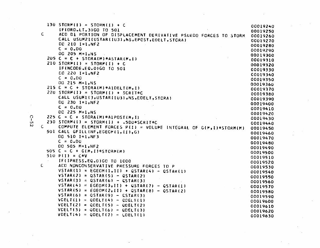
130 STORM(I) = STORM(I) + C 00019240IF(ORD.LT.3)GO TO 501 00019250
C ACD D1 PORTION OF DISPLACEMENT DERIVATIVE PSUEDO FORCES TO STORM 00019260CALL USUM21(USTAR(IU3),NS,EPOSTEOELT,STCRA) 00019270DC 210 I=1,NF2 00019280C = 0.DO 0001929000 205 M=1,NS 00019300
205 C = C + STORA(M)*ASTAR{M,I) 00019310210 STORM(I) = STORM(I) + C 00019320
IF(NCOOE.EQ.0)GO TO 501 00019330CO 220 I=1,NF2 00019340C = 0.D0 0001935000 215 M=,INS 00019360
215 C = C + STORA(M)*AIDELT(M,I) 00019370220 STORM(I) = STORM(I) + SCRIT*C 00019380
CALL USUM1(3,USTAR(IU3),NS,EDELT,STORA) 0001939000 230 I=iNF2 00019400C = 0.00 00019410DC 225 M=1,NS 00019420
0 225 C = C + STORA(M)*AIPOST(M,I) 00019430L 230 STORM(1) = STORM(I) + .500*SCRIT*C 000194.40
C COMPUTE ELEMENT FORCES P(I) = VOLUME INTEGRAL OF G(MI)*STORM(M) 00019450501 CALL GFILL(NF,EGEOP(1II),G) 00019460
DO 510 I=1,NF3 00019470C = 0.00 0001948000 505 M=1,NF2 00019490
505 C = C + G(M,I)*STORM(M) 00019500510 PI) = C*V 00019510
IF(IPRESS.EQ.O)GO TO 1000 00019520C ACC NONCONSERVATIVE PRESSURE FORCES TO P 00019530
VSTAR(1) = EGECM(1,11) + QSTAR(4) - QSTAR(1) 00019540VSTAR(2) = QSTAR(5) - QSTAR(2) 00019550VSTAR(3) = QSTAR(6) - CSTAR(3) 00019560VSTAR44) = EGEOM(3,II) + QSTAR(7) - QSTAR(1) 00019570VSTAR(5) = EGEOM(2,II) + QSTAR(8) - QSTAR(2) 00019580VSTAR(6) = QSTAR(9) - CSTAR(3) 00019590VCELT(1) = QDELT(4) - QDELT(1) 00019600VCELT(2) = QCELT(5) - (QELT(2) 00019610VCELT(3) = QDELT(6) - QDELT(3) 00019620VDELT(4) = QDELT(7) - OELT(1) 00019630
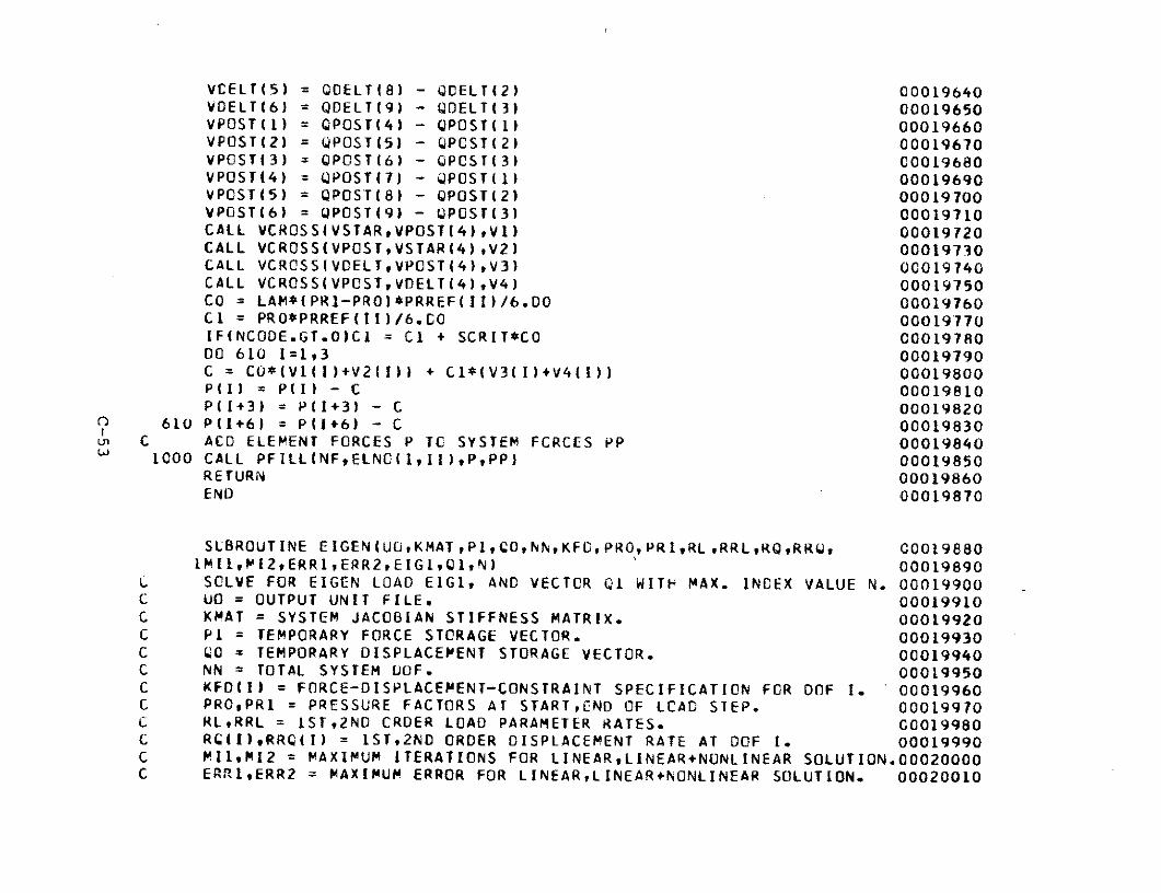
VCELT(5) = QDELT(8) - QCELT(2) 00019640VDELT(6) = QDELT(9) - QDELT(3) 00019650VPOST(1) = QPOST(4) - QPOST(1) 00019660VPOSTi2) = QPOST(5) - QPCST(2) 00019670VPOSTI3) = QPOST(6) - QPCST(3) C0019680VPOST(4) = QPOST(7) - QPOST(1) 00019690VPOST(5) = QPOST(8) - QPOST(2) 00019700VPOST(6) = QPOST(9) - QPOST(3) 00019710CALL VCROSS(VSTAR,VPOST(4),V1) 00019720CALL VCROSS(VPOST,VSTAR(4),V2) 00019730CALL VCROSS(VDELT,VPOST(4),V3) 00019740CALL VCROSS(VPOST,VDELT(4),V4) 00019750CO = LAM*(PRI-PRO)*PRREF(II)/6.DO 00019760CI = PRO*PRREF(II)/6.CO 00019770IF(NCODE.GT.0)CI = Cl + SCRIT*CO C001978000 610 1=1,3 00019790C = CO*(V1(I)+V2(Il) + CI~(V3(I)+V4(I)) 00019800P(I) = PII) - C 00019810P(1+3) = P(I+3) - C 00019820
610 P(I+61 = P(I+6) - C 00019830C ACO ELEMENT FORCES P TC SYSTEM FORCES PP 000198401000 CALL PFILL(NFELNO(I I),P,PP) 00019850
RETURN 00019860END 00019870
SLBROUTINE EIGEN(UO,KMAT,PItCO NN,KFC,PRO,PR1,RL,RRLRQtRR, 00019880IMI1,MI2,ERR1,ERR2,EIG1,Q1,N) ' 00019890
L SOLVE FOR EIGEN LOAD EIGI, AND VECTOR QI WITH MAX. INDEX VALUE N. 00019900C UO = OUTPUT UNIT FILE. 00019910C KMAT = SYSTEM JACOBIAN STIFFNESS MATRIX. 00019920C PI = TEMPORARY FORCE STORAGE VECTOR. 00019930C Q0 = TEMPORARY DISPLACEMENT STORAGE VECTOR. 00019940C NN = TOTAL SYSTEM DOF. 00019950C KFDII) = FORCE-DISPLACEMENT-CONSTRAINT SPECIFICATION FOR DOF I. 00019960C PROPR1 = PRESSURE FACTORS AT STARTEND OF LCAD STEP. 00019970C RL,RRL = ISTt2ND CRDER LOAD PARAMETER RATES. 00019980C RC(I),RRQ(I) = 1ST,2ND ORDER DISPLACEMENT RATE AT DOF I. 00019990C MIIMI2 = MAXIMUM ITERATIONS FOR LINEAR,LINEAR+NONLINEAR SOLUTION.00020000C ERR1,ERR2 = MAXIMUM ERROR FOR LINEAR,LINEAR+NONLINEAR SOLUTION. 00020010
C EIGI = CCMPUTED EIGENVALUE (CRITICAL PATH VALUE). 00020020C Q111) = ITH COMPONENT CF EIGENVECTCR (BUCKLING DISPLACEMENT). 00020030C N = DOF OF LARGEST 01 COMPONENT. 00020040
CCMMON/COMNF/NF 00020050INTEGER UOtNN,KFD(1),MII,MI2,N 00020060DOUBLE PRECISION KMAT(NNNN),P1(1),tO(1),PROPR1t 00020070IRLRRL,RQ(1),RRQ(1),ERRI,ERR2,EIGQI(l1) 00020080INTEGER I,NI 00020090DCUBLE PRECISION EIGOMAXItDL,C 00020100
201 FORMAT(1H ,'EIGENVALUE = ',015.8,5X,'DOF OF LARGEST COMPONENT OF E00020110IIGEN VECTOR = ',15) 00020120NI = 0 00020130NCODE = 0 00020140EIG 0.00DO 00020150CC 5 I=INN 00020160
5 Q1(1) = I 0002017011 EIGO = EIG1 00020180
CL = RL 00020190IF(NCODE.GT.O)DL = DL + .500DEIGO*RRL 0002020000 20 I=I,NN 0002021000(I) = Q1(I) 00020220SQ1I) = RQ(I) 00020230IF(NCODE.GT.O)Q1(1) = 0111) + .500*EIGO*RRQ(I) 00020240
20 CONTINUE 00020250CALL EIGEN1(NN,NCCE,QL,EIGOQO,OL,PROPRI,P1) 00020260NOD = NN/NF 00020270CALL OUTPQ(6,NO0,NF,P1,QO) 00020280CC 50 I=1,NN 00020290IF(KFD(I).LT.0)PI(I) = 0.D0 00020300
50 CONTINUE 00020310CALL SOLVE(KMAT,NN,KFU,PI*Ql) 00020320N = 0 00020330MAXI = O.DO 0002034000 70 I=1,NN 00020350IF(ODAS(QI(I)).LE.0ABS(MAX1))GO TO 70 00020360N = [ 00020370MAXI = 01(I) 00020380
70 CCNTINUE 00020390MAXI = 1.DC/MAXI 00020400EIGL = -MAX1 00020410
IF(KFD(N).NE.N)N = KFC(N) 00020420DC ICO I=l,NN 00020430
100 (1(I) = QL(f)*MAXx 00020440WRITE(UO,2OL)EIGIN 00020450NI = NI+1 00020460C = DABS((EIGI-EIGO)/EIGI) 00020470IF(NCODE.GT.O.ANO.(NI.GE.MI2.OR.C.LE.ERR2)|RETURN 00020480IF(NCUDE.EG.0.ANO.(NI.GE.MI.0R.C.LE.ERRI))NCODE = 1 00020490GO TO 11 00020500END 00020510
SUBROUTINE POST2(NN,QQCRITf,QDCT,CCPOST,LCRITTLDOTtPROtPRI,PP, 00020520IKODE) 00020530
C FORM 2ND ORDER POSTBUCKLING LOAD TERM PP (=P21,P22 FCR KODE=1,2). 00020540C NN = TOTAL SYSTEM DOF. 00020550C CQCRIT(I) = PREDICTED TOTAL DISPLACEMENT OF DOF I AT CRITICAL PT. 00020560C CCDOTI) = PRECICTED CISPLACEMENT RATE OF DOF I AT CRITICAL PT. 00020570C CPOST(I) = ITH DISPLACEMENT OF CRITICAL BUCKLING EIGENVECTOR. 00020580C LCRIT = PREDICTED LOAD PARAMETER VALUE AT CRITICAL POINT. 00020590C LOOT = PREDICTED LOCAD PARAMETER RATE AT CRITICAL POINT. 00C020600C PRO,PRl = PRESSURE FACTORS AT START OF LOAD STEP,CRITICAL POINT. 00020610C PP(I) = COMPUTED PSUEDC-FORCE TERM AT DOF 1. 00020620C KCDE = CODE FOR DUAL USE OF SUBROUTINE. 00020630C ORD = MAXIMUM TENSOR ORDER TO BE USED FOR DIFFERENCE EXPANSION. 00020640C NEL,NSNF = NUMBER OF ELEMENTS,STRAIN COPPONENTSDOCF PER NODE. 00020650C ELNO(J,I) = NODE NUMBERS FOR ELEMENT 1. 00020660C EGEOM(J,I) = GEOMETRIC PROPERTIES FOR ELEMENT 1. 00020670C T(I) = THICKNESS OF ELEMENT I. 00020680C IPRESS = NONCONSERVATIVE CODE = 0,1 FOR NO PRESSUREPRESSURE. 00020690C PRREF(I) = PRESSURE INTENSITY ON ELEMENT I FCR PRESSURE VECTOR. 00020700
COMCON/CCMORD/ORD/COMNEL/NEL/COMNS/NS/COMNF/NF CC020710COMMON/COMEL/ELNO/COMEG/EGEOM/COMT/T 00020720COMMON/COMIPR/IPRESS/CCMPRR/PRREF 00020730INTEGER NN,KODEORO,NELNSNFELNC(3,1),IPRESS 00020740OCUBLE PRECISION (QCRIT(1), QDOT(1),QQPOST(1),LCRIT,LDOT,PRO,PRI# 000207501PP(1),EGEOM(3,1),T(1),PRREF(1) 00020760INTEGER NF2,NF3,IU2,1U3,III,M 00020770DOUBLE PRECISION V,C,QCRIT(9),QDCT(9),QPCST(9),DCRIT(6),DDOT(6), 00020780IDPOST46),ECRIT(3),EDOT(3),EPOST(3)iACRIT(3,6),AIDOT(3,6)t 00020790
1AIPCST(3,6),STORA(3),STCOR(3),STORM(6)tG(6,9),P(9),UCRIT20O) 00020800
CCUBLE PRECISION CCClVCRIT(6),VDCT(6),VPOST(6),Vl(3)tV2(3), 00020810IV3(3).V4(3)
00020820NF2 = NF*2 00020830NF3 = NF*3 000208401U2 = 2 + NS 00020850IU3 = IU2 + NS*(NS+1)/2 0002086000 5 I=1,NN 00020870
5 PPII) = 0.D0 0002088000 1000 II=1,NEL 00020890V = .5DO*T(1I)*EGECM(1,11)*EGEOM(2,II) 000209CO
C FCRM FUNCAMENTAL CRITICAL QUANTITIES 00020910CALL QFILL(NF,ELNC(1,11),CQCRITQCRIT) 00020920
1901 FORMAT(IHO,9E14.7) 00020930
WRITEI6,1901)(QCRIT(),I=1,NF3) 00020940CALL DFILL(NFEGEOM(ltII)QCRIT,0CRIT) 00020950WRITE(6,1901)(DCRIT(I),I=1,NF2)
00020960CALL AFILL(NF,CRIT,ACRIT,1) 0002097000 1910 I=1,3 00020980
1910 WRITE(6,190i)(ACRIT(IJ) ,J=1,NF2) 00020990CALL EFILL(NF,0CRITECRIT) 00021000WRITE(6,1901)(ECRIT(I),I=1,3)
00021010C FORM STRESS-STRAIN TENSORS 00021020
CALL UFILL(IIORD,CRITUCRIT) 00021030C FCRM FUNCAMENTAL RATE QUANTITIES 00021040
CALL QFILL(NF,ELNC(1,II),QQDOTQCOT) 00021050WRITE(6l,1901)(QDOtl),l=1,NF3) 00021060CALL DFILL(NF,EGECM(1,II),C CT,0COT) 00021070WRITE(6,1901)(cOT(I),I=1,NF2) 00021080CALL AFILL(NF,IDOT,AIO0T,O) 0002109000 1920 1=1,3 00021100
1920 WRITE(6,1901)(AIDOT( 1J),J=1,NF2) 00021110DC 20 I=1,NS 00021120C = 0.00DO 00021130CC 15 M=1,NF2 00021140
15 C = C + ACRIT(IM)DDCT(M) 0002115020 EDOT(I) = C 00021160
WRITE(6,1901)(EOCT(I),I=1,3) 00021170C FCRM POSTBUCKLING EIGEN QUANTITIES 00021180
CALL QFILLiNFELNO(1,II),QQPOST,QPOST) 00021190
WRITE(6,1901)(QPCST(I),I=L,NF3) 00021200
CALL DFILLINF,EGEOM(1,II),QPOST,0PCST) 00021210
WRITE(6,1901)(DPOST(I),1=1,NF2) 00021220
CALL AFILL(NF,DPOST,AIPOST,O) 00021230
CC 1930 1=1,3 00021240
1930 WRITE(6,1901)(AIPOS(II,J),J=1,NF2) 00021250
D00 30 I=1,NS 00021260
C = .D00 00021270
00 25 M=1,NF2 00021280
25 C = C + ACRIT(I,M)*DPOST(M) 00021290
30 EPCST(I) = C 00021300
WRITE(6,1901)(EPOST(I),1I=,3) 00021310
C FORM STORM = DO PORTION OF DISPLACEMENT DERIVATIVE PSUEDO FORCES 00021320
00 104 I=1,NS 00021330
C = 0.00 00021340
DO 102 M=1,NF2 00021350
102 C = C + A100T(1,M)*DPOST(M) 00021360
104 STORB(I) = C 00021370
CALL USUMI(2tUCRIT(IU2),NS,STORBtSTORA) 00021380
DO 110 I=P1NF2 00021390
U C = 0.00 00021400
CC 105 M=1,NS 00021410
105 C = C + STORA(M)*ACRIT(M,I) 00021420
110 STORM(I) = C 00021430
WRITE(6,1901)(STORM(II9I=1,NF2) 00021440
CALL USUMI(2,UCRIT(IU2) NS,EDOCTSTCRA) 00021450
DO 120 I=1NF2 00021460
C = 0.00DO 00021470
00 115 M=1,NS 00021480
115 C = C + STORA(M)*AIPOST(M,I) 00021490
120 STORM(I) = STORM(I) + C 00021500
WRITE(6,1901)(STORM(I),I=1,NF2) 00021510
CALL USUMI(2,UCRIT(IU2),NSEPOSTSTORA) 00021520
00 130 I=1,NF2 00021530
C = 0.00 00021540
DO 125 M=1,NS 00021550
125 C = C + STORA(M)*ALDCT(M,I) 00021560
130 STORM(I) = STORM(I) + C 00021570
WRITE(619O1)(STORM(I),I=1,NF2) 00021580
IF(ORD.LT.3)GO TO 501 00021590
C ACO D01 PORTION CF OISPLACEMENT DERIVATIVE PSUEDO FORCES TO STORM 00021600CALL USUM21(UCRIT(IU3),NSEDCT,EPOST,STORA) 0002161000 210 I=1,NF2 00021620C = 0.00 00021630CC 205 M=1,NS 00021640
205 C = C + STORA(M)*ACRIT(Ml) 00021650210 STORM(I) = STORM(I) + C 00021660
C COMPUTE ELEMENT FORCES P(I) = VOLUME INTEGRAL OF G(MI)*STORM(M) 00021670501 CALL GFILL(NFEGEOM(1II),G) 00021680
00 510 I=1,NF3 00021690C = O.DO 00021700CO 505 M=1,NF2 00021710
505 C = C + GI(MI)*STORM(M) 00021720510 P(I) = C*V 00021730
WRITE(6,1901)(P(II,I=,NF3) 00021740IF(IPRESS.EQ.O)GO TO IC00 00021750
C ADD NONCONSERVATIVE PRESSURE FORCES TO P 00021760VOOT(1) = QDOT(4) - QDCT(1) 00021770VCOT(2) = QOOT(5) - QDCT(2) 00021780VDOT(3) = DOCT(6) - COCT(3) 00021790
Ln VCOT(4) = QDOT(7) - DCT(1) 00021800VCOT(5) = QDOT(8) - Q0CT(2) 00021810VCOT(6) = QDOT(9) - QOCT(3) 00021820VPOST(1) = QPOST(4) - CPOST(1) 00021830'VPOST(2) = QPOST(5) - QPCST(2) 00021840VPOST(3) = QPOST(6) - QPCST(3) 00021850VPOST(4) = QPOST(7) - QPOST(1) 00021860VPCST(5) = QPOST(8) - QPOST(2) 00021870VPOST(6) = QPOST(9) - QPOST(3) 00021880CO = (PRO + LCRIT*(PRI-PRO))*PRREF(I11/6.00 00021890C1 = 0.00 00021900CALL VCROSS(VOOT,VPOST(4),Vl) 00021910CALL VCROSSIVPOST,VDOT(4),V2) 00021920IF(KODE.EQ.2)GO TO 601 00021930VCRIT(1) = EGECM(1,I) + QCRIT(4) - QCRIT(1) 00021940VCRIT(2) = QCRIT(5) - QCRIT(2) 00021950VCRIT(3) = QCRIT(6) - QCRIT(3) 00021960VCRIT(4) = EGEOM(3,1I) + QCRIT(7) - QCRIT(1) 00021970VCRIT(5) = EGECM(2,Il) + QCRIT(B) - QCRIT(2) 00021980VCRIT(6) = QCRIT(9) - QCRIT(3) 00021990
C1 = LDOT*(PR1-PR)*PRREF(II)/6.DO 00022C00CALL VCROSS(VCRITVPOST(4),V3) 00022010CALL VCROSS(VPOST,VCRIr(4),V4) 00022020
601 00 610 I=1,3 00022030C = CO*(VlII)+V2(I)) + CI*(V3(I)+V4(I)) 00022040Pil) = P(l) - C 00022050P(I+3) = P(I+3) - C 00022060
610 P(1+6) = P(I+6) - C 00022070C ACC ELEMENT FORCES P TO SYSTEM FCRCES PP 000220801000 CALL PFILL(NFELNC(1,II),P,PP) 00022090
RETURN 00022100END 00022110
SUBROUTINE POST3(NN,QQCRITQQDGTlCQPOS1,QQDCT2,QQPOS2,SPOST1, 00022120ILCRITLDOTlLDOT2,PROPR1,PP) 00022130
C FCRM 3RD ORDER POSTBUCKLING LOAD TERM PP. 00022140C NN = TOTAL SYSTEM OF. 00022150C QCRITIl) = PREDICTED TOTAL DISPLACEMENT OF COF I AT CRITICAL PT. 00022160C QDOTl(i) = CRITICAL 1ST ORDER DISPLACEMENT RATE AT COF I. CC0022170
n C CQPOS1(I) = ITH EIGENVECTOR VALUE (1ST ORDER POSTBUCKLING RATE). 00022180C QQDOT2(1) = CRITICAL 2ND ORDER DISPLACEMENT RATE AT COF I. C0022190C QQPCS2(I) = ITH VALUE OF 2ND ORDER POSTBUCKLING DISPLACEMENt. 00022200C SPOSTI = IST ORDER FUNCAMENTAL PATH RATE* 00022210C LCRIT = PREDICTED LOAD PARAMETER VALUE AT CRITICAL POINT. 00022220C LDOT1 = IST ORDER LOAD PARAMETER RATE AT CRITICAL POINT. 00022230C LOCT2 = 2ND ORDER LOAC PARAMETER RATE AT CRITICAL POINT. 00022240C PRO,PR1 = PRESSURE FACTORS AT START CF LOAD STEPCRITICAL POINT. 00022250C PP(I) = COMPUTED PSUEDC FORCE TERM AT DOF I. 00022260C ORD = MAXIMUM TENSOR ORDER TO BE USED FOR DIFFERENCE EXPANSION. 00022270C NELNS,NF = NUMBER OF ELEMENTS,STRAIN COMPONENTS,DOF PER NODE. 00022280C ELNO(J,I) = NODE NUMBERS FOR ELEMENT 1. 00022290C EGEOP(JI) = GEOMETRIC PROPERTIES FOR ELEMENT I. 00022300C T(I) = THICKNESS OF ELEMENT 1. 00022310C IPRESS = NONCONSERVATIVE CODE = 0,I FQR NO PRESSURE,PRESSURE. 00022320C PRRCF(I) = PRESSURE INTENSITY ON ELEMENT I FCR PRESSURE VECTOR. 00022330
CGMPCN/COMORD/ORD/COMNEL/NEL/COMNS/NS/COMNF/NF 00022340COMMON/COMEL/ELNC/COMEG/EGEOM/COMT/T 00022350CCMMON/COMIPR/IPRESS/CCMPRR/PRREF 00022360INTEGER NNORDNELtNStNF,ELNO(3,1),IPRESS 00022370
DOUBLE PRECISION CCCRIT(1),Q0OTl(1), QPCS1(1),QQCT2(1), 00022380ICQPOS2(1),SPOSTILCRIT,LDOTItLDOc2,PROoPRIPP(I),EGECM(3,1),T(1), 000223902PRREF(1) 00022400INTEGER NF2tNF3,tU2IIUIU3,IIM 00022410CCUBLE PRECISION VCQCRIT(9),QDOTif9)tQPOST1(9),QCOT2(9), 00022420IQPOST2(9),OCRIT(6),00OT1(6),0POSTI(6),COCT2(6),DPOST2(6), 000224302ECRIT(3),EDOTI(3),tPOSTI(3),EDOT2(3),EPOST2(3)tACRIT(3,6), 000224403 AICOT1( 3 ,6 ),AIPOSL(3,6),AIOoT2(3,6),AlPOS2(3t6),STORA(3)tSTORB(3),
0 0 0 2 24 5 04STORM(6),G(6,9),P(9),UCRIT(20) 00022460DCUBLE PRECISION COtCLC2,VCRIT(6),VDOT1(6),VPOSTI(6),VDOT2(6), 000224701VPOST2(6),VI(3),V2(3),V3(3),V4(3),VS(3),V6(3)tV7(3),V8(3),V9(3), 000224802V10(3),V11(3),V12(3),V13(3) C0022490NF2 = NFe2 00022500NF3 = NF*3 000225101I2 = 2 + NS 00022520IU3 = IU2 + NS*(NS+1)/2 00022530DO 5 I=1,NN 00022540
5 PP(I) = 0.00 0002255000 1000 II=1,NEL 00022560V = .5DO*T(II)*EGECM(1,II)*EGEOM(2,II) 00022570
o~ FORM FUNDAMENTAL CRITICAL QUANTITIES 00022580CALL QFILL(NFELNO(ItII),QQCRIT,QCRIT) 00022590
CALL DFILL(NFEGEOM(t1II),QCRIT,CCRIT) 00022600CALL AFILL(NF,CCRIT,ACRIT,1) 00022610CALL EFILL(NFDCRITECRIT) 00022620
C FORM STRESS-STRAIN TENSORS C0022630CALL UFILL(IICROCR RI,ECRIT) 00022640C FCRM 1ST ORDER FUNCAPENTAL RATE QUANTITIES 00022650CALL QFILL(NF,ELNC(1,I1),QQDOTIQOOTI) 00022660CALL UFILL(NFEGEOM(1,ill),DCTI,CCCT1) 00022670CALL AFILL(NF,CDOTI,AD100T1,) 00022680DO 20 I=1NS 00022690C = 0.D0 00022700CC 15 M=1,NF2 00022710
15 C = C + ACRIT(I,M)*DDOTI(M) 0002272020 EDOTHI) = C 00022730
C FCRM IST ORDER POSTBUCKLING RATE QUANTITIES 00022740CALL QFILL(NF,ELNO(1,1lI)QQPOSI,QPCSTI) 00022750CALL OFILL(NF,EGEOM(1,I),QPOSTI,DPOSTI) 00022760CALL AFILL(NFz0POST1,A1POS1,O) 00022770
00 30 I=1,NS 00022780C = 0.00 0002279000 25 M=1,NF2 00022800
25 C = C + ACRIT(I,M)*DPOSTI(M) 0002281030 EPOSTI1) = C 00022820
C FORM 2ND ORDER FUNDAMENTAL RATE QUANTITIES 00022830CALL wFILL(NF,ELNC(1,II),QCCT2,(CCT2) 00022840CALL DFILL(NFEGEGM(1,II),QDOT2,oCT2) 00022850CALL AFILLINF,000T2,AIOT2,0) 00022860DC 40 I=1,NS 00022870C = O.DO 00022880CC 35 M=1,NF2 00022890
35 C = C + ACRIT(I,M)*DDOT2(M) + A100TI(I,M)*CDCTI(M) 0002290040 ECOT2(I) = C 00022910
C FORM 2ND ORDER POSTBUCKLING RATE QUANTITIES 00022920CALL QFILL(NFELNC(1,II),QQPCS2,QPOST2I C0022930CALL OFILL(NF,EGEOM(1,II),QPOSr2,DPOST2) 00022940CALL AFILL(NFDPOST2,A1POS2,0) 00022950DC 50 I=1,NS 00022960C = 0.00 00022970DO 45 M=1,NF2 00022980
45 C = C + ACRIT(.IM)*DPOST2(M) + AIPOSL(IM)*(CPOSTIfM) + 2.00* 00022990ISPOSTI*CDOTI(M)) 00023000
50 EPOST2(I) = C 00023010C FORM STORM = DO PORTION OF DISPLACEMENT CERIVATIVE PSUEDO FORCES 00023020
00 104 I=1,NS 00023030C = O.DO 00023040CC 102 M=I,NF2 C0023050
102 C = C + AIPOSI(IM)*CDCT2(M) 00023060104 STORB(I) = C 00023070
CALL USUMI(2,UCRITilU2)tNSSTTORA) 0002308000 110 I=I,NF2 00023090C = 0.DO 00023100CC 105 M=1,NS 00023110
105 C = C + STORA(M)*ACRIT(M,I) 00023120110 STORM(I) = SPOSTL**2*C 00023130
CALL USUMI(2,UCRIIT(IU2),NS,EPOST,STORA) C0023140DC 120 I=1,NF2 00023150C = 0.00 00023160DO 115 M=1,NS 00023170
115 C = C + STORA(M)*A1OOT2(M,I) 00023180120 STORM(I) = STORM(I) + SPOST1**2*C 00023190
CALL USUM1(2,UCRIT(IU2),NS,EDOT2,STORA) 0002320000 130 I=1,NF2 00023210C = 0.DO 00023220DO 125 M=1,NS 00023230
125 C = C + STORA(M)*A1POS1(M,I) 00023240130 STORM(1) = STORM(I) + SPOST1**2*C 00023250
00 134 I=1,NS 00023260C = 0.DO 00023270DC 132 M=1,NF2 00023280
132 C = C + AIDOT1(I,v)*DPOST2(M) 00023290134 STORB(1) = C 00023300
CALL USUM1(2,UCRIT(IU2),NS,STORBSIORA) C0023310DC 140 I=1,NF2 00023320C = 0.D0 00023330CC 135 M=1,NS 00023340
135 C = C + STORA(M)*ACRIT(,I) 00023350140 STORM(i) = STORM() + SPOST1*C 00023360
CALL USUMI(2,UCRITIU2),NS,EDOT1,STORA) 00023370CC00 150 I=1,NF2 00023380C = 0.00DO 0002339000 145 M=1,NS 00023400
145 C = C + STORA(M)*AIPOS2(M,I) 00023410150 STORM(I) = STORM(1) + SPOST1*C 00023420
CALL USUMI(2,UCRIf(IU2),NSEPOST2,STORA) 00023430CC 160 I=1,NF2 00023440C = 0.00 000234500C 155 M=1,NS 00023460
155 C = C + STORA(M)*AIDOT1(M,I) 00023470160 STORM(1) = STORM(I) + SPCSTI*C 00023480
DO 164 I=I,NS 00023490C = 0.00 00023500CC 162 M=1,NF2 00023510
162 C = C + AIPOSI(IP)*DPOST2(M) 00023520164 STORB(I) = C 00023530
CALL USUM1(2,UCRIT(IU2),NS,STORB,STORA) 00C023540DC 170 I=1,NF2 00023550C = 0.00 00023560DO 165 M=1.NS 00023570
165 C = C + STORA(M)*ACRIT(P,I) 00023580170 STORII) = STORM(I) + C 00023590
CALL USUMI(2,UCRIT(IU2),NSEPOST1,STCRA) CC023600CO 180 I=1,NF2 00023610C = 0.00DO 0002362000 175 M=t1NS 00023630
175 C = C + STORA(M)*A1POS2(M,I) 00023640180 STORM(I) = STORM(I) + C 00023650
CALL USUM1(2,UCRIT(IU2),NS,EPCST2,STORA) 00023660DO 190 I=1,NF2 00023670C = C.DO 00023680DC 185 M=1,NS 00023690
185 C = C + STORA(M)*AIPCSI(M,I) 00023700190 STORM(I) = STORM(I) + C 00023710
IF(ORD.LT.3)GO TO 501 00023720C ACD Cl PORTION OF DISPLACEMENT DERIVATIVE PSUEDO FORCES TO STORM 00023730
CALL USUM21(UCRIT(IU3),NS,EPCST1,EDOT2,STORA) 00023740DC 210 I=1,NF2 00023750C = 0.00 00023760DO 205 M=I1NS 00023770
205 C = C + STCRA(M)*ACRIT(M,I) 00023780210 STORM(I) = STORMfI) + SPOST1**2*C 00023790
CALL USUM1(3,UCRIT(IU3),NS,EDOTI,STORA) 00023800DC 220 I=L,NF2 00023810C = 0.D00 00023820DO 215 M=1,NS 00023830
215 C = C + STORA(M)*AlPOS1(M,I) 00023840220 STORM(I) = STORM(I) + SPOSTI**2*C 00023850
CALL USUM21(UCRIT(IU3),NSEPOSTI,ErDOTI,STORA) 00023860DO 230 I=1,NF2 00023870C = 0.00 00023880DO 225 M=1,NS 00023890
225 C = C + STORA(M)*A00OTI(M,I) 00023900230 STORM(I) = STORM(I) + 2.D00*SPOSTL**2*C 00023910
CALL USUM21(UCRIT(IU3)tNSEDOCT1sEPCST2,STCRA) 0002392000 240 I=1,NF2 00023930C = 0.00DO 00023940DC 235 M=1,NS 00023950
235 C = C + STORA(M)*ACRIT(MI) 00023960240 STORM(I) = STORM(I) + SPOSTI*C 00023970
CALL USUMI(3,UCRII(IU3)tNSEPOSTlTSTORA) 0002398000 250 I=1,NF2 00023990C = 0.00 00024000CC 245 M=1,NS 00024010
245 C = C + STORA(M)*A100DI(M,I) 00024020250 STORMI() = STORM(1) + SPOSTI*C 00024030
CALL USUM21(UCRIT(IU3),NS,EOCT,EPCST1,STORA) 00024040CCD 260 I=1,NF2 00024050C = 0.DO 00024060DO 255 M=1,NS 00024070
255 C = C + STORA(M)*AlPOSI(M,1) 00024080260 STORM(I) = STORM(I) + 2.00*SPOSTI*C 00024090
CALL USUM21(UCRIT(IU3),NSEPCST1,EPOST2,STORA) 00024100CC 270 I=1,NF2 00024110C = 0.00DO 0002412000 265 M=1,NS 00024130
265 C = C + STCRA(M)*ACRIT(M,I) 00024140270 STORMI) = STORM(I) + C 00024150
CALL USUMI(3,UCRIT(IU3),NS,EPOSTISTORA) 0002416000 280 I=19NF2 00024170C = 0.00 00024180DC 275 M=1,NS 00024190
275 C = C + STORA(M)*AIPOS1(M,I) 00024200280 STORMil) = STORM(1) + C 00024210
C CCMPUTE ELEMENT FORCES P(l) = VOLUME INTEGRAL OF G(V,I)*STORM(M) 00024220501 CALL GFILL(NF,EGEOM(,lll),G) -00024 230
DC 510 I=1,NF3 00024240C = 0.00DO 0002425000 505 M=1,NF2 00024260
505 C = C + G(M,I)*STORM(M) 00024270510 PIl) = C*V 00024280
IF(IPRESS.EQ.O)GO TO ICCO0 00024290C ACD NONCONSERVATIVE PRESSURE FORCES TO P 00024300
VCRIT(1) = EGECM(1,II) + QCRIT(4) - QCRIT(1) 00024310VCRIT(2) = QCRIT(5) - QCRIT(2) 00024320VCRIT(3) = QCRIT(6) - QCRIT(3) 00024330VCRIT(4) = EGEOM(3,II) + QCRIT(7) - QCRIT(1) 00024340VCRIT45) = EGEOM(2,II) + QCRIT(8) - QCRIT(2) 00024350VCRIT(6) = QCRIT(9) - QCRIT(3) 00024360VCOTI(1) = QDOT1(4) - 0OTI(1) 00024370
VCOTI(2) = QOOTI(5) - QOT1(2) 00024380
VCOT1(3) = QDOT1(6) - QCCT1(3) 00024390
VOT1(4) = QDOT1(7) - 00.T(1) 00024400
VCOTI(5) = QOTI(8) - QDCT1(2) 00024410
VDCOT(6) = QDOTI(9) - QDOTI(3) 00024420
VPOSTI(1) = QPOSTI(4) - QPOST1(1) 00024430
VPCST1(2) = OPOSTI(5) - QPOST1(2) 00024440
VPOSTI(3) = QPOST1i6) - QPOST1(3) 00024450
VPOST1(4) = QPOST1(7) - QPOSTI(1) 00024460
VPOSTI(5) = OPOST1(8) - QPOST1(2) 00024470
VPCSTI(6) = QPOSTI(9) - QPCST1(3) 00024480
VCOT2(1) = QDOT1(4) - QDOTI(1) 00024490
VOOT2(2) = QDOTI(5) - 00OTI12) 00024500
VCCT2(3) = ~0CT1(6) - QCOTL(3) 00024510
VOOT2(4) = QOO71(7) - Q0CTI(1) 00024520
VDOT2(5) = QDOT1(8) - QDOTl(2) 00024530
VCOT2(6) = QDOT1(9) - QCOTI(3) 00024540
VPOST2(1) = QPOST2(4) - QPOCST2(1) 00024550
VPOST2(2) = QPCST2(5) - QPOST2(2) 00024560
SVPOST2(3) = QPOST2(6) - QPOST2(3) 00024570I VPOST2(4) = QPOST2(7) - QPOST2(l) 00024580Ln VPOST2(5) = QPOST2(8) - QPOST2(2) 00024590
VPOST2(6) = QPOST2(9) - QPOST2(3) 00024600
CO = (PRO + LCRIT*(PRI-PRO))*PRREF(11)/6.DO 00024610
Cl = LOOT1*(-PRO)*PRREF(II)/6.00 00024620
C2 = LDOT2*(PRI-PRO)*PRREF(II)/6.DO 00024630
CALL VCROSS(VDCT2,VPOST1(4),Vl) 00024640
CALL VCRCSS(VPOST1,VD0T2(4)tV2) 00024650
CALL VCRCSS(VDOT1,VPOST1(4),V3) 00024660
CALL VCROSS(VPOSTI,VDOTI(4),V4) 00024670
CALL VCROSSIVCRITVPOST (4),V5) 00024680
CALL VCROSS(VPCST1,VCRIT(4),V6) 00024690
CALL VCROSS(VOTI,VPOST2(4),V7) 00024700
CALL VCROSS(VPOST2,VDOT1(4),V8) 00024710
CALL VCROSS(VCRIT,VPOST2(4),V9) 00024720
CALL VCROSS(VPCST2,VCRIT(4),VIO) 00024730
CALL VCROSS(VPOST1,VPOSTI(4),VIL) 00024740
CALL VCRCSS(VPOST2,VPOST1(4),V12) 00024750
CALL VCROSS(VPOSTI,VPOST2(4),V13) 00024760
00 610 1=1,3 00024770
C = CO*(V1I()+V2(1)+V7(1)+VV8(II+V2(13()) C1*(2.DO*V3(I) 000247801+2.DO*V4(1)+V9(1)+VIO(I)+2.DO*VIl(1)) + C2*(V5(I)+V6(11)) 00024790P(I) = P1I) - C 00024800PI1+3) = PII+3) - C 00024810
610 P(1+6) = P11+6) - C 00024820C ACDD ELEMENT FORCES P TO SYSTEM FORCES PP 000248301000 CALL PFILLNFELNO(1,II)tPPP) 0C024840
RETURN 00024850END 00024860
SUBROUTINE PRATES(KMAT,PICl,P2,t2,NNtPCSTKFD,SCRIT, 000248701QCCRIT,QQDOT1,QQDCT2,LCRITtLOOT1,LDOT2,PROtPRI, 000248802CQPOStLPOSTICQPOS2,LPOST2,QQPOS3) 00024890
C COMPUTE POSTBUCKLING RATES FOR LOCAD PARAMETER AND DISPLACEMENTS. 00024900C KMAT = SYSTEM JACOBIAN STIFFNESS MATRIX. 00024910C P1tQItP29Q2 = TEMPORARY STORAGE VECTORS. 00024920C NN = TOTAL SYSTEM DOF. 00024930C IPOST = COF OF LARGEST EIGENVECTOR COMPONENT. 00024940C 'KFD(1) = FORCE-DISPLACEMENT-CONSTRAINT SPECIFICATION FOR DOF 1. 00024950C SCRIT = PREDICTED CRITICAL VALUE CF FUNDAMENTAL PATH. 00024960C QCCRIT(I) = PREDICTED CRITICAL VALUE OF DISPLACEMENT AT DOF I. 00024970C CQDOT1II),QQDOT2(I) = IST,2ND ORDER CRITICAL FUNDAMENTAL 00024980C DISPLACEMENT RATE AT COF 1. 00024990C LCRIT = PREDICTED CRITICAL VALUE OF LOAD PARAMETER. 00025000C LCOT1,L00T2 = IST,2ND ORDER CRITICAL LOAD PARAMETER RATES. 00025010C PRO,PR1 = PRESSURE FACTORS AT START OF LOAD STEP,CRITICAL POINT. 00025020C LPCSTI,LPOST2 = COMPUTEC IST,2ND ORDER PCSTBLCKLING LOAD RATES. 00025030C QPOSOS(IhCQPOS2(1)tQQPOS3() = 1ST,2ND,3RD CRDER POSTBUCKLING 00025040C DISPLACEMENT RATES AT DOF 1. 00025050C NF = DOF PER NODE. 00025060
CCMMON/COMNF/NF 00025070INTEGER NN,IPOSTKFD(1) 00025080DOUBLE PRECISION KMAT(NN,NN),P(1),Q1(1i),P2(1),Q2(1),SCRIT, 000250901QQCRIT(1),0QDOTI(1),QQDOT2(1),LCRITtLOOT,LOCT2,PROtPRl, 000251002QCPOSI(1),LPOSTI,CCPOS2(1),LPOST2,C4POS3(1) 00025110INTEGER I 00025120DOUBLE PRECISION CNCD,SPOST1,SPOST2 00025130
C SOLVE FOR 1ST ORDER DISPLACEMENTS 00025140DO 10 I=1,NN 00025150
10 PHI() = 0.00 00025160P11IPOST) = 1.00DO 00025170CALL SOLVE(KMATtNNKFD,P1,QQPOSI) 00025180NCC = NN/NF 00025190CALL OUTPQ(6,NOD,NF,P1,QQPOS1) 00025200
C SOLVE FOR IST ORDER LOADS AND 2ND ORDER DISPLACEMENTS 00025210CALL POST2(NN,CQCRIT,(OCTL,#CQPOS1,LCRIT,LOCT1,PRO,PRI,P1,1) 00025220CALL POST2(NN,QQCRITQQPOS1,CQPOS1,LCRIT,LDOTIPRO,PRltP2,2) 00025230CALL OUTPQ(6,NOD,NF,PI,P2) 00025240CN = 0.00 00025250CC = 0.00 00025260DC 110 I=1,NN 00025270CN = CN + QQPOSI(I)*P2(I) 00025280
110 CC = CD * CQPOS1(I)*P1Il) 00025290SPOSTI = -. 500*CN/CD 00025300LPOSTL = LDOTI*SPOST1 00025310DC 120 I=1,NN 00025320IF(KF(I).GT.O)GC TO 120 00025330PI(l) = 0.00 00025340P2(I) = 0.00 00025350
120 CCNTINUE 00025360CALL SOLVE(KMAT,NNKFC,PI,Q1) 00025370CALL SOLVE(KMAT,NN,KFD,P2,Q2) 00025380CALL OUTPQ(6,ND,NF,P1,P2) 00025390CALL OUTPQ(6,NODtNF,QI,Q2) 0002540000 130 I=1,NN 00025410
130 QQPOS2(I) = -(2.DO*SPOST1*1(Il) + Q2(I)) 00025420CALL OUTPQf6,NODNF,QQCCT2,QQPOS2) 00025430
C SOLVE FOR 2ND ORDER LOADS AND 3RD ORDER DISPLACEMENTS 00025440CALL POST3(NN,QQCRIT,QCDOTI,CQPOS1,QQDOT2,CQPCS2,SPOST1, 00025450ILCRIT,LDOTI,LDOT2,PR0,PRIP2) 00025460CALL OUTPQ(6,NODNF,QQCRITtP2) 00025470CALL OUTPQ(6,NOD,NF,QQUCTiQQPOSI) 00025480CN = 0.00 0002549000 210 I=1,NN 00025500
210 CN = CN + CQPOS1(I)*P2(I) 00025510SPOST2 = -CN/CD 00025520LPOST2 = LDOTI*SPOST2 + LDCT2*SPCSTI**2 00025530DO 220 II1,NN 00025540IF(KFD(I).GT.0)GO TO 220 00025550
P2(1) = 0.00 00025560220 CONTINUE 00025570
CALL SOLVE(KMAT,NNvKF0,P2,Q2) 00025580CALL OUTPQ(6,NOONFP2t,2) 00025590CO 230 I=INN 00025600
230 C4POS3(I) = -3.DO*(SPOST2*QI(I) + Q2(I)) 00025610CALL OUTPQ(6,NOD,NFQQPOS3,QQPOS3) 00025620RETURN 00025630DEBUG INIT(SPOSTILPOSTI,SPOST2,LPCST2,CN,CD) 00025640END 00025650
DOUBLE PRECISION FUNCTION VDOT(V1,V2) 00025660C COMPUTE VECTOR DOCT PRODUCT VCOT = VI DOT V2. C0025670
DOUBLE PRECISION V1(1),V2(1) 00025680VDOT = VlI)*V2(1) + VI(2)*V2(2) + V(I3)*V2(3) 00025690RETURN 00025700END 00025710
SSUBROUTINE VCROSS(VLIV2tVV) 00025720o C COMPUTE VECTOR CROSS PRODUCT Vl X V2 = VV. 00025730
CCUBLE PRECISION V(),V2(1),VV(1) 00025740VV(1) = Vl(2)*V2(3) - VI(3)*V2(2) 00025750VV(2) = V1(3)*V2(1) - Vl(I)*V2(3) 00025760VV(3) = Vl(1)*V2(2) - V1(2)*V2(1) 00025770RETURN 00025780END 00025790
COUBLE PRECISION FUNCTION VLENTH(V) 00025800C COMPUTE VLENTH = LENGTH OF VECTOR V. 00025810
COUBLE PRECISION V(1) 00025820VLENTH = DSQRT(V(I)**2 + V(2)**2 + V(3)**2) 00025830RETURN 00025840END 00025850
SUBROUTINE VNORM(V,VV) 00025860C COMPUTE NORMALIZED UNIT VECTOR VV FROM GIVEN VECTOR V. 00025870
CCUBLE PRECISION V(I),VV(1),C 00025880C = OSQRTIV(I)**2 + V(2)**2 + V(3)**2) 00025890IF(C.LE.0.DO)C = 1.DO 00025900VV(1) = V(1)/C 00025910VVI2) = V(2)/C 00025920VV(3) = V(3)/C 00025930RETURN 00025940END 00025950
SUBROUTINE MERGE(KVAT,ELNOKFDNEL, N,NF) 00025960C GENERATE AND MERGE ELEMENTAL MATRICES INTO GLOBAL MATRIX KMAT. 00025970C ASSUMES ELEMENTS HAVE 3 NODES, MATRICES MAY BE UNSYMMETRIC. 00025980C KMAT = GLOBAL (TCTAL SYSTEM) MATRIX, WHICH MAY BE UNSYMMETRIC. 00025990C ELNO(JI) = NODE NUMBERS FOR ELEMENT I. 00026000C KFD(I) = FORCE-DISPLACEMENT-CONSTRAINT SPECIFICATION FOR DOF I. 00026010C KFU(I) = +,- = SPECIFIED FORCE,DISPLACEMENT. 00026020C KFD(I) = +-I INDICATES INDEPENDENT DOF. C0026030C KFD(I) = +-J INDICATES DEPENDENT FREEDOM WHOSE DISPLACEMENT IS 00026040C CONSTRAINED TO EQUAL DISPLACEMENT AT J. 00026050C NEL = NUMBER OF ELEMENTS. 00026060
) C NN = TOTAL SYSTEM DOF = NUMBER OF NODES TIMES NF. 00026070C NF = DOF PER NODE. 00026080C GENER8 ROUTINE GENERATES ELEMENTAL MATRIX. 00026090
INTEGER ELNO(3l),KFD(1),NEL,NN,NF 00026100OCUBLE PRECISION KPAT(NNNN) 00026110INTEGER IE,IJ.IItJJtIOJO,IIOJJC,IP,JP,IN,JNILOCIILOC 00026120DOUBLE PRECISICN K(9,9) C0026130
C ZERO OUT GLOBAL MATRIX 0002614000 5 II=1,NN 00026150D00 5 JJ=1,NN 00026160
5 KMAT(II,JJ) = 0.00 0002617000 100 IE=1,NEL 00026180CALL GENER8(IE,K) 00026190
C IPJP ARE PARTITION ROWtCOLUMN NUMBERS. 00026200DO 100 IP=1,3 00026210IN = ELNO( IP,IE) 0002622010 = NF*IP - NF 00026230II0 = NF*IN - NF 00026240DO 100 JP=1,3 - 00026250
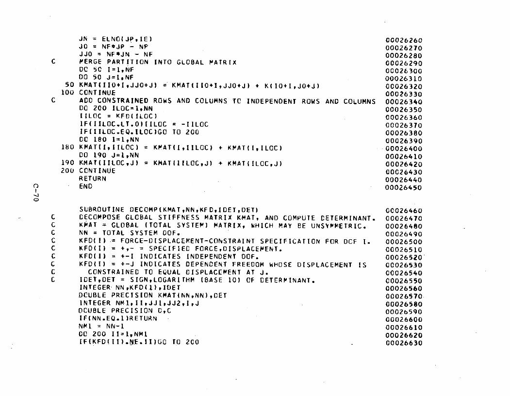
JN = ELNO(JPIE) 00026260JO = NF*JP - NP 00026270JJO = NF*JN - NF 00026280
C MERGE PARTITION INTO GLOBAL MATRIX 00026290DO 50 I=1,NF 00026300DO 50 J=1,NF 00026310
50 KMAT(IIO+IJJO+J) = KMAT(110+IJJO+J) + K(IO+IJO+J) 00026320100 CONTINUE 00026330
C ACD CONSTRAINED ROWS AND COLUMNS TO INDEPENDENT ROWS AND COLUMNS 00026340DG 200 ILOC=1,NN 00026350IILOC = KFO(ILOC) 00026360IF(IILOC.LT.O)IILOC = -IILOC 00026370IFIILOC.EQ.ILOC)GO TO 200 00026380CC 180 I=1,NN 00026390
180 KMAT(IIILOC) = KMAT(IIILOC) + KMAT(I,ILOC) -00026400DO 190 J=1,NN 00026410
190 KMAT(IILOC,J) = KMAT(IILOCJ) + KMAT(ILOCJ) 00026420200 CONTINUE 00026430
RETURN 00026440END 00026450
SUBROUTINE DECOMP(KMAT tNNKF DI DET ,DET) 00026460C DECOMPOSE GLOBAL STIFFNESS MATRIX KMAT, AND COMPUTE CETERMINANT. 00026470C KMAT = GLOBAL (TOTAL SYSTEM) MATRIXt WHICH MAY BE UNSYMETRIC. 00026480C NN = TOTAL SYSTEM DOF. 00026490C KFD(I) .= FORCE-DISPLACEMENT-CONSTRAINT SPECIFICATION FOR DCF I. 00026500C KFD(I) = +,- = SPECIFIED FORCE,DISPLACEMENT. 00026510C KFO(I) = +-I INDICATES INDEPENDENT DOF. 00026520'C KFD(I) = +-J INDICATES DEPENDENT FREEDOM WHOSE DISPLACEMENT IS 00026530C CONSTRAINED TO EQUAL DISPLACEMENT AT J. 00026540C IDETtDET = SIGNLOGARITHM (BASE 10) OF DETERMINANT. 00026550
INTEGER NNKFD(1),IDET 00026560DOUBLE PRECISION KMAT(NN,NN),DET 00026570-INTEGER NMltll,JJJJ2,I,J 00026580DOUBLE PRECISION D,C 00026590IF(NN.EQ.1)RETURN 00026600NM1 = NN-1 00026610DO 200 II=1,NMI 00026620IF(KFD(II).NE.II)GO TO 200 00026630
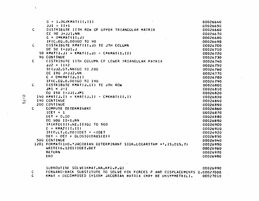
O = 1.DO/KMAT(II1II) 00026640JJ1 = II+1 00026650
C DISTRIBUTE IITH ROW OF UPPER TRIANGULAR MATRIX 00026660CC 90 J=JJ1,NN 00026670C = O*KMAT(IIJ) 00026680IF(C.EQ.O.DO)GO TO 90 00026690
C DISTRIBUTE KMAT(II,J) TO JTH COLUMN 00026700DC 50 I=JJI,J 00026710
50 KMAT(I,J) = KMAT(IJ) - C*KMAT(l,II) 0002672090 CONTINUE 00026730
C CISTRIBUTE IITH COLUMN CF LOWER TRIANGULAR VATRIX 00026740JJ2 = II+2 00026750IF(JJ2.GT.NN)GO TO 200 00026760DC 190 J=JJ2,NN 00026770C = D*KMAT(J,II) 00026780IF(C.EQ.0.DO)GO TO 190 00026790
C DISTRIBUTE KMAT(J,II) TC JTH ROW 00026800JMI = J-1 00026810DO 150 I=JJIJMI 00026820
150 KMAT(J,I) = KMAT(Jl) - C*KMAT(III) 00026830190 CONTINUE 00026840200 CONTINUE 00026850
C COMPUTE DETERMINANT 00026860ICET = 1 00026870DET = 0.00 00026880DO 500 II=t1NN 00026890IF(KFD(II).NE.I)GO TO 500 00026900C = KMA,T(II,II) 00026910IFID.LT.C.0O)IDET = -IDET 00026920DET = DET + DLOGIO(DABS(D)) 00026930
500 CONTINUE 000269401201 FORMAT(IHO',JACOBIAN DETERMINANT SIGN,LOGARITHM =0,15,D15.7) 00026950
WRITE(6,201)IDETDET 00026960RETURN 00026970END 00026980
SUBROUTINE SOLVE(KMATNNKFDP,Q) 00026990C FCRWARC-BACK SUBSTITUTE TO SOLVE FOR FORCES P AND DISPLACEMENTS Q.00027000C KMAT = DECOMPOSED SYSTEM JACOBIAN MATRIX (MAY BE UNSY@METRIC). 00027010
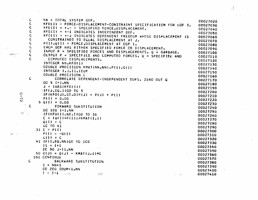
C NN = TOTAL SYSTEM DOF. 00027020C KFD(I) = FORCE-DISPLACEMENT-CONSTRAINT SPECIFICATION FOR DOF I. 00027030C KFD(I) = +,- = SPECIFIED FORCEtDISPLACEMENT. 00027040C KFC(I) = +-I INDICATES INDEPENDENT DOF. 00027050C KFD(I) = +-J INDICATES DEPENDENT FREEDOM WHOSE DISPLACEMENT IS 00027060C CONSTRAINED TO EQUAL DISPLACEMENT AT J. 00027070C P(I),Q(I) = FORCE,DISPLACEMENT AT COF 1. 00027080C EACH DOF HAS EITHER SPECIFIED FORCE OR DISPLACEMENT. 00027090C INPUT P = SPECIFIED FORCES AND DISPLACEMENTS, Q = GARBAGE. 00027100C OUTPUT P = SPECIFIED AND CCMPUTED FORCES, Q = SPECIFIED AND C0027110C COMPUTED DISPLACEMENTS. C0027120
INTEGER NNKFD(1) 00027130DCUBLE PRECISION KMAT(NN,NN),P(1),C(1I) 00027140INTEGER I,J,Il,ICUM 00027150DOUBLE PRECISION C 00027160C CORRELATE DEPENDENT-INDEPENDENT DOFS, ZERO OUT Q 0002717000 5 I=I,NN 00027180J = IABS(KFO(I)) 00027190-IF(J.EQ.I)GO TO 5 00027200IFIKFD(J).GT.O)P(J) = P(J) + P(I) 00027210PII) = 0.00 00027220
5 Q(I) = O.DO 00027230C FORWARD SUBSTITUTION 00027240
DO 100 I=1,NN 00027250IF(KFD(I).NE.I)GO TO 31 00027260C = (Q(I)+P(I))/KMAT(I,I) 00027270Q(I) = C 00027280GC TO 41 00027290
31 C = P(i) 00027300P(1) = -Q(1) 00027310.(I) = C 00027320
41 IF(I.EQ.NN)GO TO ICO 0002733011 = 1+1 00027340DC 50 J=I1,NN 00027350
50 Q(J) = Q(J) - KMAT(JI)*C 00027360100 CONTINUE 00027370
C BACKWARD SUBSTITUTION 00027380I = NN+I 00027390DO 200 IDUM=r1NN 00027400I = I-1 .- C - - 0002741-0
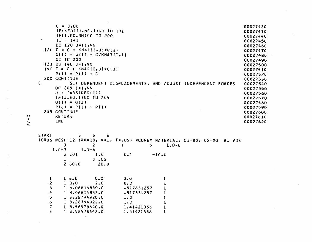
C = 0.00 00027420IF(KFD(I).NE.I)GO TO 131 00027430IF(I.EQ.NN)GO TO 200 0002744011 = 1+1 00027450DC 120 J=IINN 00027460
120 C = C + KMAT(I,J)* cJ) 00027470Q(I) = Q(I) - C/KAT(I,I) 00027480GC TO 200 00027490
131 DC 140 J=I,NN 00027500140 C = C + KMAT(IJ)*Q(J) 00027510
P(I) = P(I) + C 00027520200 CCNTINUE 00027530
C SET DEPENDENT DISPLACEMENTS, AND ADJUST INDEPENDENT FORCES 00027540DC 205 I=1,NN 00027550J = IABS(KFD(I)) 00027560IF(J.EQ.I)GO TO 205 00027570W(1) = Q(J) 00027580P(J) = P(J) - P(I) 00027590
205 CCNTINUE 00027600RETURN 00027610ENC 00027620
START 5 5 6TCRUS VESP-12 (RR=10, R=.2, T=.05) MOONEY MATERIAL, CI=80, C2=20 R. VOS
3 2 1 5 1.0-6I.C-3 1.0-6
2 .01 1.0 0.1 -10.01 3 .052 60.0 20.0
1 1 8.0 0.0 0.0 12 1 8.0 2.0 0.0 13 1 8.06814830.0 .517631257 14 1 8.06814832.0 .517631257 15 1 8.26794920.0 1.0 16 1 8.26794922.0 1.C 17 1 8.58578640.0 1.41421356 18 1 8.58578642.0 1.41421356 1
9 1 9.0 0.0 1.7320508110 1 9.0 2.0 1.7320508111 1 9.48236870.0 1.9318516512 1 9.48236872.0 1.9318516513 110.0 0.0 2.014 110.0 2.0 2.,015 110.51763130.0 1.9318516516 110.51763132.0 1.9318516517 111.0 0.0 1.7320508118 111.0 2.0 1.7320508119 111.41421360.0 1.4142135620 111.41421362.0 1.4142135621 111. 73205080.0 1.022 111.73205082.0 1.023 111.93185170.0 .51763125724 111.93185172.0 .51763125725 112.0 0.0 0.026 112.0 2.0 0.0
1 2 2 1 32 2 3 4 23 2 4 3 64 2 5 6 35 2 6 5 76 2 7 8 67 2. 8 7 10-8 2 9 10 79 2 10 9 11
10 2 11 12 1011 2 12 11 1412 2 13 14 1113 2 14 13 1514 2 15 16 1415 -2 16 15 1816 2 17 18 1517 2 18 17 1918 2 19 20 1819 2 20 19 2220 2 21 22 1921 2 22 21 23

22 2 23 24 2223 2 24 23 2624 2 25 26 23
1 3 2 3 25 3 26 31 2 3 2 5 2 7 29 2 11 2 13 2 15 2
17 2 19 2 21 2 23 225 2 2 2 4 2 6 28 2 10 2 12 2 14 216 2 18 2 20 2 22 224 2 26 2
2 1 1 1 4 1 3 1 4 3 3 31 5 1 6 3 5 3 8 1 7 1 8 3 7 3
10 1 9 1 10 3 9 3 12 1 11 1 12 3 11 314 1 13 1 14 3 13 3 16 1 15 1 16 3 15 3lb 1 17 1 18 3 17 3 20 1 19 1 20 3 19 322 1 21 1 22 3 21 3 24 1 23 1 24 3 23 326 1 25 1
2
11 1.0 2 1.0 3 1.0 4 1.05 1.0 6 1.0 7 1.0 8 1.09 1.0 10 1.0 11 1.0 12 1.0
13 1.0 14 1.0 15 1.0 16 1.017 1.0 18 1.0 19 1.0 20 1.021 1.0 22 1.0 23 1.0 24 1.0
80.10.51.02.03.04.04.55.0