Embed Size (px)
Citation preview

Development of Seismic Isolation Systems Using Periodic Materials
Nuclear Energy Enabling Technologies Dr. Yi-‐Lung Mo
University of Houston
In collabora3on with: University of Texas-‐Aus5n
Prairie View A&M University Argonne Na5onal Laboratory
Alison Hahn, Federal POC Ron Harwell, Technical POC
Project No. 11-3219
DEVELOPMENT OF SEISMIC ISOLATION SYSTEMS USING
PERIODIC MATERIALS
TECHNICAL REPORT
Project No. 3219
By
Yiqun Yan and Y.L. Mo
University of Houston
Farn-Yuh Menq and Kenneth H. Stokoe, II
The University of Texas at Austin
Judy Perkins
Prairie View A & M University
Yu Tang
Argonne National Laboratory
Performed in cooperation with the Department of Energy
September 2014
Department of Civil and Environmental Engineering
University of Houston
Houston, Texas

ii
iii
DISCLAIMER
This research was performed in cooperation with the Department of Energy
(DOE), the University of Texas at Austin, Prairie View A&M University, and Argonne
National Laboratory. The contents of this report reflect the views of the authors, who are
responsible for the facts and accuracy of the data presented herein. The contents do not
necessarily reflect the official view or policies of the DOE. This report does not
constitute a standard, specification, or regulation, nor is it intended for construction,
bidding, or permit purposes. Trade names were used solely for information and not
product endorsement.

v
ACKNOWLEDGEMENTS
This research, Project No. 3219, was financially supported by the Department of
Energy NEUP NEET-1 Program. Alison Hahn Krager (Federal Manager), Jack Lance
(National Technical Director), and Ron Harwell (Technical POC) served as the project
monitoring committee.

vii
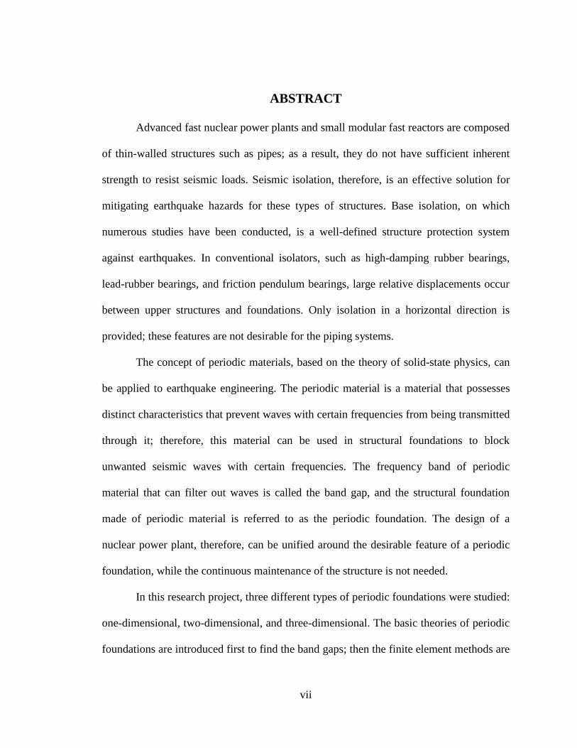
ABSTRACT
Advanced fast nuclear power plants and small modular fast reactors are composed
of thin-walled structures such as pipes; as a result, they do not have sufficient inherent
strength to resist seismic loads. Seismic isolation, therefore, is an effective solution for
mitigating earthquake hazards for these types of structures. Base isolation, on which
numerous studies have been conducted, is a well-defined structure protection system
against earthquakes. In conventional isolators, such as high-damping rubber bearings,
lead-rubber bearings, and friction pendulum bearings, large relative displacements occur
between upper structures and foundations. Only isolation in a horizontal direction is
provided; these features are not desirable for the piping systems.
The concept of periodic materials, based on the theory of solid-state physics, can
be applied to earthquake engineering. The periodic material is a material that possesses
distinct characteristics that prevent waves with certain frequencies from being transmitted
through it; therefore, this material can be used in structural foundations to block
unwanted seismic waves with certain frequencies. The frequency band of periodic
material that can filter out waves is called the band gap, and the structural foundation
made of periodic material is referred to as the periodic foundation. The design of a
nuclear power plant, therefore, can be unified around the desirable feature of a periodic
foundation, while the continuous maintenance of the structure is not needed.
In this research project, three different types of periodic foundations were studied:
one-dimensional, two-dimensional, and three-dimensional. The basic theories of periodic
foundations are introduced first to find the band gaps; then the finite element methods are

viii
used, to perform parametric analysis, and obtain attenuation zones; finally, experimental
programs are conducted, and the test data are analyzed to verify the theory. This
procedure shows that the periodic foundation is a promising and effective way to mitigate
structural damage caused by earthquake excitation.
ix
TABLE OF CONTENTS
DISCLAIMER ................................................................................................................... iii ACKNOWLEDGEMENTS ................................................................................................ v ABSTRACT ...................................................................................................................... vii TABLE OF CONTENTS ................................................................................................... ix
LIST OF FIGURES .......................................................................................................... xv LIST OF TABLES ........................................................................................................ xxvii 1 INTRODUCTION ....................................................................................................... 1
1.1 Significance of Research ........................................................................... 1
1.2 Objective of Report ................................................................................... 3
1.3 Scope of the Research ............................................................................... 4
2 LITERATURE REVIEW ............................................................................................ 7 2.1 Overview of Base Isolation Systems ......................................................... 7
2.1.1 The passive base isolation system........................................................ 7
2.1.2 The active base isolation system ........................................................ 11
2.2 Overview of Phononic Crystals............................................................... 12
2.2.1 History of phononic crystals .............................................................. 13
2.2.2 Computing methods of phononic crystals.......................................... 17
2.2.3 Application of phononic crystals ....................................................... 19
2.3 Overview of Periodic Structures ............................................................. 20
3 THE BASIC THEORIES OF PERIODIC FOUNDATIONS ................................... 27 3.1 Basic Theories of 1D Layered Periodic Foundations.............................. 27
3.2 Basic Theories of 2D Periodic Foundations ............................................ 31
3.3 Basic Theory of 3D Periodic Foundations .............................................. 38
x
3.3.1 Basic equations of elastic wave ......................................................... 38
3.3.2 Finite difference time domain method ............................................... 39
3.3.3 Theoretical solutions of 3D test specimens by COMSOL ................. 45
4 FINITE ELEMENT MODELING OF PERIODIC FOUNDATIONS ..................... 47 4.1 FE Modeling of 1D Layered Periodic Foundations ................................ 47
4.1.1 Parametric study of 1D periodic foundations .................................... 47
4.1.2 FE modeling of 1D periodic foundations using ABAQUS ............... 54
4.2 FE Modeling of 2D Periodic Foundations .............................................. 58
4.2.1 FE modeling of 2D periodic foundations using COMSOL ............... 58
4.2.2 FE modeling of 2D periodic foundations using ABAQUS ............... 61
4.3 FE Modeling for 3D Periodic Foundations ............................................. 64
4.3.1 FE modeling of 3D periodic foundations using COMSOL ............... 64
4.3.2 FE modeling of 3D periodic foundations using ABAQUS ............... 68
5 EXPERIMENTAL PROGRAM ................................................................................ 73
5.1 Experimental Program of 1D Layered Periodic Foundations ................. 73
5.1.1 1D layered periodic foundations specimen and test setup ................. 73
5.1.2 Test procedure of 1D layered periodic foundations ........................... 75
5.2 Experimental Program of 2D Periodic Foundations ............................... 76
5.2.1 2D periodic foundation specimen materials ...................................... 76
5.2.2 2D periodic foundations specimen design ......................................... 79
5.2.3 Formwork design ............................................................................... 84
xi
5.2.4 Test setup of 2D periodic foundations ............................................... 85
5.2.5 Test procedure of 2D periodic foundations ....................................... 88
5.3 Experimental Program of 3D Periodic Foundations ............................... 90
5.3.1 3D periodic foundation specimen materials ...................................... 90
5.3.2 3D periodic foundation specimen design ........................................... 94
5.3.3 Formwork design ............................................................................... 95
5.3.4 Manufacture procedure ...................................................................... 98
5.3.5 Test setup of 3D periodic foundations ............................................. 101
5.3.6 Test procedure of 3D periodic foundations ..................................... 105
6 EXPERIMENTAL RESULTS ................................................................................ 109 6.1 Experimental Results of 1D Layered Periodic Foundations ................. 109
6.1.1 Ambient vibration test results .......................................................... 109
6.1.2 Seismic test results ........................................................................... 110
6.1.3 Harmonic test results........................................................................ 113
6.2 Experimental Results of 2D Periodic Foundations ............................... 114
6.2.1 S wave test results of 2D periodic foundations ................................ 114
6.2.2 P wave test results of 2D periodic foundations ................................ 122
6.3 Experimental Results of 3D periodic foundations ................................ 127
6.3.1 Shear wave tests ............................................................................... 127
6.3.2 Primary wave tests ........................................................................... 144
7 COMPARISON OF TEST RESULTS AND ANALYTICAL OUTCOMES ........ 159
xii
7.1 Comparison of 1D Layered Periodic Foundations ................................ 159
7.1.1 Comparison of theoretical band gaps and attenuation zones for 1D
periodic foundations ................................................................................................ 159
7.1.2 Comparison of time history analysis and test results for the 1D
periodic foundations ................................................................................................ 160
7.2 Comparison of 2D Periodic Foundations .............................................. 162
7.2.1 Comparison of theoretical band gaps and attenuation zones for the 2D
periodic foundations ................................................................................................ 162
7.2.2 Comparison of scanning frequency analysis and the test results for 2D
periodic foundations ................................................................................................ 163
7.2.3 Comparison of time history analysis and test results for the 2D
periodic foundations ................................................................................................ 165
7.3 Comparison of the 3D Periodic Foundations ........................................ 166
7.3.1 Comparison of theoretical band gaps and attenuation zones for the 3D
periodic foundations ................................................................................................ 166
7.3.2 Comparison of scanning frequency analysis and test results for the 3D
periodic foundations ................................................................................................ 167
7.3.3 Comparison of time history analysis and test results for the 3D
periodic foundations ................................................................................................ 169
8 CONCLUSIONS AND SUGGESTIONS ............................................................... 171 8.1 Conclusions ........................................................................................... 171
8.2 Suggestions............................................................................................ 172

xiii
9 REFERENCES ........................................................................................................ 174 A APPENDIX: Design Guidelines for Periodic Foundations ..................................... 187
A.1 Design Procedures ................................................................................. 187
A.2 Design Example .................................................................................... 187
A.3 Back-up Information ............................................................................. 188
A.4 References ............................................................................................. 190

xv
LIST OF FIGURES
Fig. 1.1 Reflection of wave possessing a frequency falling within the frequency band gap
of the periodic material[1]
.................................................................................................... 2
Fig. 1.2 Wave propagation of wave possessing a frequency outside of the frequency band
gap of the periodic material[1]
............................................................................................. 2
Fig. 1.3 Logic path of the research ..................................................................................... 4
Fig. 2.1 Testing elastomeric bearings[3]
.............................................................................. 8
Fig. 2.2 Friction pendulum bearing used in Benicia-Martinez Bridge[18]
......................... 10
Fig. 2.3 1D, 2D and 3D phononic crystals[29]
................................................................... 13
Fig. 2.4 Sculpture by Eusebio Sempere[35]
....................................................................... 15
Fig. 2.5 Bent wave-guide and absolute value of the displacement field for the guiding
mode[51]
............................................................................................................................. 17
Fig. 2.6 Phononic spectrum[29]
.......................................................................................... 20
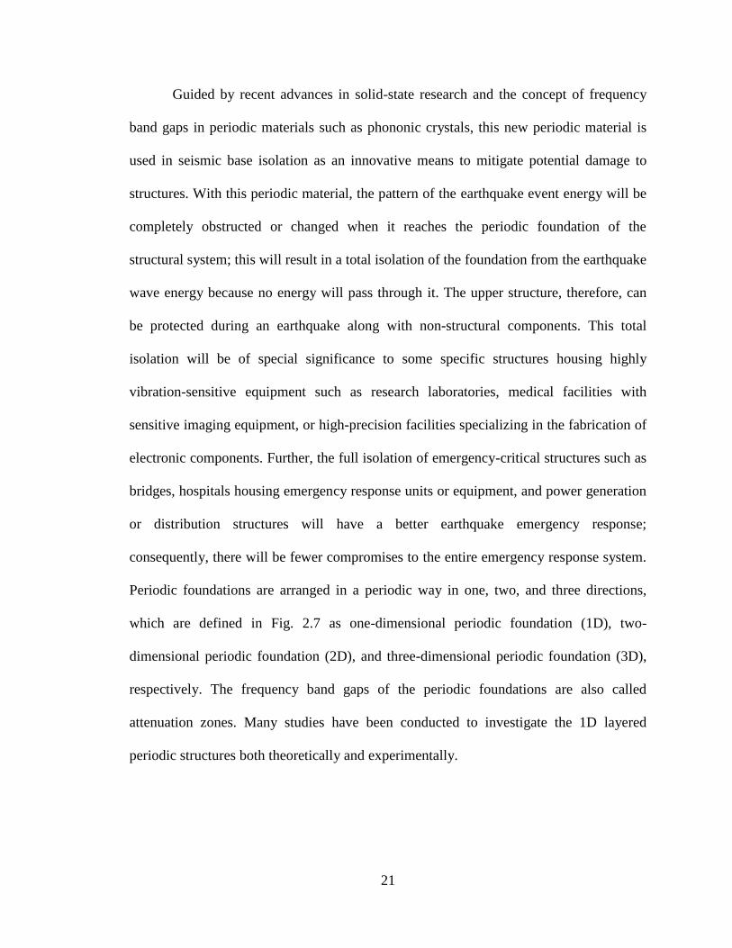
Fig. 2.7 (a) Periodic foundation with upper structure; (b) 1D periodic foundation; (c) 2D
periodic foundation; (d) 3D periodic foundation. ............................................................. 22
Fig. 2.8 Oil and gas offshore platform .............................................................................. 23
Fig. 2.9 Large scale experiment of 2D periodic structure to shield surface elastic waves[86]
........................................................................................................................................... 25
Fig. 3.1 Configuration of a layered periodic foundation and its unit cell ......................... 28
Fig. 3.2 Dispersion curves of 1D periodic foundation ...................................................... 28
Fig. 3.3 A three-components square lattice periodic structure ......................................... 32
Fig. 3.4 Brillouin zone of 2D periodic structures ............................................................. 37
xvi
Fig. 3.5 The first Brillouin zone of 2D periodic structures ............................................... 37
Fig. 3.6 Theoretical solution of the first band gap of 2D periodic foundation ................. 37
Fig. 3.7 The unit of the grids in the FDTD method[63]
...................................................... 41
Fig. 3.8 Theoretical band gap for 3D periodic foundation solved by COMSOL ............. 45
Fig. 4.1 One unit cell of 1D periodic structure ................................................................. 48
Fig. 4.2 Young’s modulus of rubber vs. the first band gap with longitudinal wave ......... 49
Fig. 4.3 Young’s modulus of concrete vs. the first band gap with longitudinal wave ..... 49
Fig. 4.4 Density of concrete vs. the first band gap with longitudinal wave...................... 50
Fig. 4.5 Density of rubber vs. the first band gap with longitudinal wave ......................... 50
Fig. 4.6 Young’s modulus of rubber vs. the first band gap with transverse wave ............ 51
Fig. 4.7 Young’s modulus of concrete vs. the first band gap with transverse wave ......... 51
Fig. 4.8 Density of concrete vs. the first band gap with transverse wave ......................... 51
Fig. 4.9 Density of rubber vs. the first band gap with transverse wave ............................ 51
Fig. 4.10 Thickness ratio vs. the starting frequency of first band gap with longitudinal
wave .................................................................................................................................. 53
Fig. 4.11 Thickness ratio vs. the starting frequency width of first band gap with
longitudinal wave .............................................................................................................. 53
Fig. 4.12 Unit cell size vs. first band gap with longitudinal wave .................................... 53
Fig. 4.13 Thickness ratio vs. the starting frequency of first band gap with transverse wave
........................................................................................................................................... 54
Fig. 4.14 Thickness ratio vs. the starting frequency width of first band gap with
transverse wave ................................................................................................................. 54
Fig. 4.15 Unit cell size vs. first band gap with transverse wave ....................................... 54
xvii
Fig. 4.16 The boundary conditions of 1D periodic foundation under S wave .................. 57
Fig. 4.17 The boundary conditions of 1D periodic foundation under P wave .................. 57
Fig. 4.18 FRF of node A under S wave ............................................................................ 58
Fig. 4.19 FRF of node A under P wave ............................................................................ 58
Fig. 4.20 One unit cell of 2D periodic foundation ............................................................ 59
Fig. 4.21 Core density vs. the first band gap .................................................................... 60
Fig. 4.22 Young’s modulus of rubber layer vs. the first band gap ................................... 60
Fig. 4.23 β vs. the first band gap ....................................................................................... 61
Fig. 4.24 f vs. the first band gap ........................................................................................ 61
Fig. 4.25 Boundary condition of 2D periodic foundation under S wave .......................... 64
Fig. 4.26 FRF of node A in S wave .................................................................................. 64
Fig. 4.27 Boundary conditions of 2D periodic foundation under P wave ........................ 64
Fig. 4.28 FRF of node A in P wave .................................................................................. 64
Fig. 4.29 One unit cell of 3D periodic foundation ............................................................ 65
Fig. 4.30 Core density vs. the first band gap .................................................................... 66
Fig. 4.31 Young’s modulus of rubber vs. the first band gap ............................................ 66
Fig. 4.32 Filling ratio vs. the first band gap ...................................................................... 67
Fig. 4.33 β vs. the first band gap ....................................................................................... 67
Fig. 4.34 Boundary conditions under S wave ................................................................... 69
Fig. 4.35 FRF under S wave ............................................................................................. 70
Fig. 4.36 Boundary conditions under P wave ................................................................... 70
Fig. 4.37 FRF under P wave ............................................................................................. 71
Fig. 4.38 Simplification of 3D periodic foundations ........................................................ 71
xviii
Fig. 4.39 FRF of node A under S wave ............................................................................ 72
Fig. 4.40 FRF of node A under P wave ............................................................................ 72
Fig. 5.1 Test setup for 1D periodic foundation ................................................................. 74
Fig. 5.2 Sensor arrangement for 1D periodic foundation test ........................................... 75
Fig. 5.3 Sensor arrangement for 1D periodic foundation test top view ............................ 75
Fig. 5.4 Soft neoprene (Duro10) ....................................................................................... 77
Fig. 5.5 Rubber compressive test system .......................................................................... 77
Fig. 5.6 Stress-strain relationship of rubber samples ........................................................ 78
Fig. 5.7 Top view of iron core cylinder ............................................................................ 79
Fig. 5.8 Elevation view of iron core cylinder ................................................................... 79
Fig. 5.9 Test specimens of 2D periodic foundation tests .................................................. 80
Fig. 5.10 Reinforcement of Specimen D .......................................................................... 82
Fig. 5.11 Cross-section 2-2 of Specimen D ...................................................................... 82
Fig. 5.12 Frame dimension and welding ........................................................................... 83
Fig. 5.13 Rebar cage of the RC footing ............................................................................ 84
Fig. 5.14 Unit cells in formwork of 2D periodic foundations .......................................... 85
Fig. 5.15 Picture of field test setup using T-Rex .............................................................. 86
Fig. 5.16 Layout of test setup under S wave excitations using T-Rex.............................. 86
Fig. 5.17 Test setup for S wave excitations ...................................................................... 87
Fig. 5.18 Layout of test setup under S wave excitation using Rattler .............................. 87
Fig. 5.19 Accelerometer arrangement for P wave tests .................................................... 88
Fig. 5.20 Layout of test setup under P wave excitations .................................................. 88
Fig. 5.21 Test setup for P wave excitations ...................................................................... 88
xix
Fig. 5.22 Hardness comparison in different scales[105]
..................................................... 91
Fig. 5.23 Ultra-soft polyurethane compression test setup................................................. 92
Fig. 5.24 Stress-strain relationship for polyurethane and rubber ...................................... 92
Fig. 5.25 Cast iron cube .................................................................................................... 93
Fig. 5.26 Cast iron with polyurethane wrapping............................................................... 94
Fig. 5.27 Test specimens of 3D periodic foundation tests ................................................ 95
Fig. 5.28 Formwork design ............................................................................................... 96
Fig. 5.29 Rebar design of the specimen ............................................................................ 97
Fig. 5.30 Cross-section A-A of Specimen F ..................................................................... 97
Fig. 5.31 Cross-section B-B of specimens E and F .......................................................... 98
Fig. 5.32 Formwork and cages .......................................................................................... 98
Fig. 5.33 Level formworks................................................................................................ 99
Fig. 5.34 Apply form release oil ....................................................................................... 99
Fig. 5.35 Formwork and rebar cages for Specimen E ..................................................... 100
Fig. 5.36 Coupling nuts in control specimen .................................................................. 100
Fig. 5.37 Formwork and rebar cages for Specimen F ..................................................... 100
Fig. 5.38 Casting specimens ........................................................................................... 101
Fig. 5.39 Curing of concrete ........................................................................................... 101
Fig. 5.40 Accelerometers arrangement of specimens E and F ........................................ 103
Fig. 5.41 Layout of test setup under S wave excitation .................................................. 103
Fig. 5.42 Test setup for S wave excitation ...................................................................... 103
Fig. 5.43 Picture of field test setup using........................................................................ 104
Fig. 5.44 Layout of test setup.......................................................................................... 104
xx
Fig. 5.45 Layout of test setup under P wave excitation .................................................. 105
Fig. 5.46 Test setup for P wave excitation ...................................................................... 105
Fig. 6.1 Dynamic responses induced by ambient vibration ............................................ 110
Fig. 6.2 OROVILLE/A-ORV037 in time domain .......................................................... 111
Fig. 6.3 OROVILLE/A-ORV037 in frequency domain ................................................. 111
Fig. 6.4 Vertical relative displacement at the top of the frames under OROVILLE/A-
ORV037 .......................................................................................................................... 111
Fig. 6.5 Horizontal acceleration responses at the top of the frames under 1975 Oroville
earthquake ....................................................................................................................... 112
Fig. 6.6 Vertical displacement time history at the top of the frames under 1975 Oroville
earthquake ....................................................................................................................... 112
Fig. 6.7 Horizontal acceleration on top of the frame with harmonic excitation ............. 113
Fig. 6.8 Accelerations at the top of specimens C and D ................................................. 115
Fig. 6.9 Transfer function for specimens C and D .......................................................... 115
Fig. 6.10 Ratio of transfer function ................................................................................. 116
Fig. 6.11 Acceleration in X direction on the top of the frame under a sine wave of 50Hz
......................................................................................................................................... 116
Fig. 6.12 Acceleration in X direction on the top of the frame under modified Bishop (Rnd
Val) P0486/MCG-UP with the main frequency of 50Hz................................................ 117
Fig. 6.13 Acceleration in X direction on the top of the frame under modified Bishop (Rnd
Val) P0486/MCG-360 with the main frequency of 50Hz ............................................... 117
Fig. 6.14 Modified Bishop (Rnd Val) P0486/MCG-UP in frequency domain ............... 118
Fig. 6.15 Modified Bishop (Rnd Val) P0486/MCG-360 in frequency domain .............. 118
xxi
Fig. 6.16 Accelerations in X direction at the top of each of both specimens C and D ... 118
Fig. 6.17 Transfer function for both specimens C and D................................................ 118
Fig. 6.18 Ratio of transfer function ................................................................................. 119
Fig. 6.19 Acceleration in X direction on the top of the frame under sine wave of 46 Hz
......................................................................................................................................... 120
Fig. 6.20 Accelerations in X direction on the top of the frame under sine wave of 20Hz
......................................................................................................................................... 120
Fig. 6.21 Acceleration in X direction on the top of the frame under modified
BORAH.AS/HAU000 with a main frequency of 46Hz .................................................. 122
Fig. 6.22 Acceleration in X direction on the top of the frame under modified
BORAH.AS/HAU090 with a main frequency of 46Hz .................................................. 122
Fig. 6.23 Acceleration in X direction on the top of the frame under modified
LANDERS/LCN-UP with a main frequency of 46Hz .................................................... 122
Fig. 6.24 Acceleration in Y direction on the top and bottom of Specimen D ................ 124
Fig. 6.25 Transfer function of Specimen D .................................................................... 124
Fig. 6.26 Phase differences of P wave excitation ........................................................... 124
Fig. 6.27 Acceleration in Y direction under a sine wave of 72.6Hz ............................... 125
Fig. 6.28 Acceleration in Y direction under a sine wave of 36Hz .................................. 125
Fig. 6.29 Accelerations of core cylinders in different positions under 72.6Hz .............. 126
Fig. 6.30 Acceleration in Y direction under modified Bishop (Rnd Val) P0486/MCG-UP
......................................................................................................................................... 126
Fig. 6.31 Acceleration in Y direction under modified Bishop (Rnd Val) P0486/MCG-360
......................................................................................................................................... 126
xxii
Fig. 6.32 Transfer function between the top of the steel column and RC footing .......... 128
Fig. 6.33 Transfer function ratio of the steel column for the specimens ........................ 128
Fig. 6.34 Transfer function between the top of concrete of periodic foundation and RC
footing ............................................................................................................................. 129
Fig. 6.35 Transfer function ratio of the top of concrete for the specimens ..................... 129
Fig. 6.36 Comparison of ratio of transfer function ......................................................... 130
Fig. 6.37 Acceleration at the top and bottom of concrete of the periodic foundation .... 130
Fig. 6.38 Acceleration at the top of the steel column under a sine wave 35.1Hz ........... 131
Fig. 6.39 Acceleration at the top of the concrete under a sine wave 35.1Hz .................. 131
Fig. 6.40 Acceleration in middle of the concrete under a sine wave 35.1Hz ................. 132
Fig. 6.41 Acceleration at the top of the concrete under a sine wave 52Hz ..................... 132
Fig. 6.42 Acceleration in X direction at the top of the column under modified
BORAH.AS/HAU090 with a main frequency of 35.1Hz ............................................... 134
Fig. 6.43 Acceleration in X direction at the top of concrete under modified
BORAH.AS/HAU090 with a main frequency of 35.1Hz ............................................... 134
Fig. 6.44 Acceleration in X direction in the middle of the concrete under modified
BORAH.AS/HAU090 with a main frequency of 35.1Hz ............................................... 134
Fig. 6.45 Transfer function on top of the column of Specimen F under 2V and 4.5V
excitation ......................................................................................................................... 136
Fig. 6.46 Transfer function amplitude ratio on top of the column under 2V and 4.5V
excitation ......................................................................................................................... 136
Fig. 6.47 Transfer function amplitude ratio on top of the concrete under 2V and 4.5V
excitation ......................................................................................................................... 136
xxiii
Fig. 6.48 Input acceleration of the two specimens.......................................................... 137
Fig. 6.49 Input acceleration in the frequency domain .................................................... 137
Fig. 6.50 Input acceleration after modification ............................................................... 138
Fig. 6.51 Acceleration on top of the column under 2V fixed sine S wave 43.7 Hz ....... 139
Fig. 6.52 Acceleration on top of the concrete under 2V fixed sine S wave 43.7 Hz ...... 139
Fig. 6.53 Acceleration on middle of the concrete under 2V fixed sine S wave 43.7 Hz 140
Fig. 6.54 Acceleration on top and bottom of the column under 2V fixed sine S wave 43.7
Hz .................................................................................................................................... 140
Fig. 6.55 Acceleration on top of the column under 4.5V fixed sine S wave of 43.7 Hz 141
Fig. 6.56 Acceleration on top of the concrete under 4.5V fixed sine S wave of 43.7 Hz141
Fig. 6.57 Acceleration on middle of the concrete under 4.5V fixed sine S wave of 43.7 Hz
......................................................................................................................................... 142
Fig. 6.58 Acceleration on top of the concrete under 4.5V fixed sine S wave of 43.7 Hz142
Fig. 6.59 Acceleration on top of the column of the two specimens under 2V modified
BORAH.AS/HAU000 ..................................................................................................... 144
Fig. 6.60 Acceleration on top of the column and input of Specimen F under 2V modified
BORAH.AS/HAU000 ..................................................................................................... 144
Fig. 6.61 Acceleration on top of the column of the two specimens under 4.5V modified
BORAH.AS/HAU000 ..................................................................................................... 144
Fig. 6.62 Acceleration on top of the column and input of Specimen F under 4.5V
modified BORAH.AS/HAU000 ..................................................................................... 144
Fig. 6.63 Transfer function between the top of the steel column and RC footing .......... 146
Fig. 6.64 Transfer function ratio of the top of the steel column of the specimens ......... 146
xxiv
Fig. 6.65 Transfer function between the top of the concrete of periodic foundation and
RC footing ....................................................................................................................... 146
Fig. 6.66 Transfer function ratio of the top of concrete of the specimens ...................... 146
Fig. 6.67 Acceleration at the top of the steel column in specimens E and F .................. 148
Fig. 6.68 Acceleration at the top of concrete in specimens E and F ............................... 148
Fig. 6.69 Acceleration in middle of concrete in specimens E and F at the frequency of
21.2Hz ............................................................................................................................. 148
Fig. 6.70 Acceleration at the top of the steel column in specimens E and F at the
frequency of 38.9Hz........................................................................................................ 148
Fig. 6.71 Acceleration at the top of the steel column in specimens E and F .................. 149
Fig. 6.72 Acceleration at the top of the concrete in specimens E and F ......................... 149
Fig. 6.73 Transfer function amplitude ratio on top of the column under 2V and 4.5V
excitation ......................................................................................................................... 151
Fig. 6.74 Transfer function on top of the concrete of Specimen F under 2V and 4.5V
excitation ......................................................................................................................... 151
Fig. 6.75 Transfer function amplitude ratio on top of the concrete under 2V and 4.5V
excitation ......................................................................................................................... 151
Fig. 6.76 Acceleration on top of the column under 2V fixed sine P wave 21.2 Hz ....... 153
Fig. 6.77 Acceleration on top of the concrete under 2V fixed sine P wave 21.2 Hz ...... 153
Fig. 6.78 Acceleration on middle of the concrete under 2V fixed sine P wave 21.2 Hz 153
Fig. 6.79 Acceleration on top of the column under 4.5V fixed sine P wave 21.2 Hz .... 155
Fig. 6.80 Acceleration on top of the concrete under 4.5V fixed sine P wave 21.2 Hz ... 155
Fig. 6.81 Acceleration on middle of the concrete under 4.5 fixed sine P wave 21.2 Hz 155
xxv
Fig. 6.82 Acceleration on top of the column of the two specimens under 2V modified
BORAH.AS/HAU000 P wave ........................................................................................ 156
Fig. 6.83 Acceleration on top of the concrete of the two specimens under 2V modified
BORAH.AS/HAU000 P wave ........................................................................................ 156
Fig. 6.84 Acceleration on middle of the concrete of the two specimens under 2V modified
BORAH.AS/HAU000 P wave ........................................................................................ 157
Fig. 6.85 Acceleration on top of the column of the two specimens under 4.5V modified
BORAH.AS/HAU000 P wave ........................................................................................ 158
Fig. 6.86 Acceleration on top of the concrete of the two specimens under 4.5V modified
BORAH.AS/HAU000 P wave ........................................................................................ 158
Fig. 6.87 Acceleration on middle of the concrete of the two specimens under 4.5V
modified BORAH.AS/HAU000 P wave......................................................................... 158
Fig. 7.1 Attenuation zones of 1D periodic foundation and band gaps in S wave excitations
......................................................................................................................................... 160
Fig. 7.2 Attenuation zones of 1D periodic foundation and band gaps in P wave excitations
......................................................................................................................................... 160
Fig. 7.3 Comparison of test results and FEM simulation outcomes under 1975 Oroville
earthquake ....................................................................................................................... 162
Fig. 7.4 Attenuation zones of 2D periodic foundation and band gaps in S wave excitations
......................................................................................................................................... 163
Fig. 7.5 Attenuation zones of 2D periodic foundation and band gaps in P wave excitations
......................................................................................................................................... 163
Fig. 7.6 Comparison of test results and FEA outcomes in S wave excitations............... 164
xxvi
Fig. 7.7 Comparison of test results and FEA outcomes in P wave excitations............... 165
Fig. 7.8 Comparison of test results and FEA outcomes in S wave with 46Hz excitation
......................................................................................................................................... 166
Fig. 7.9 Comparison of test results and FEA outcomes in S wave with
BORAH.AS/HAU000 ..................................................................................................... 166
Fig. 7.10 Attenuation zones of 3D periodic foundation and band gaps in S wave
excitation ......................................................................................................................... 167
Fig. 7.11 Attenuation zones of 3D periodic foundation and band gaps in P wave
excitation ......................................................................................................................... 167
Fig. 7.12 Comparison of test results and FEM simulation outcomes in S wave excitation
......................................................................................................................................... 168
Fig. 7.13 Comparison of test results and FEM simulation outcomes in P wave excitation
......................................................................................................................................... 169
Fig. 7.14 Comparison of test results and FEM simulation outcomes in S wave with
35.1Hz excitation ............................................................................................................ 170
Fig. 7.15 Comparison of test results and FEM simulation outcomes with modified
BORAH.AS/HAU090 excitation .................................................................................... 170
Fig. A.1 One unit cell of 2D periodic foundation[1]
........................................................ 188
Fig. A.2 Dispersion relationship of a coated cube inclusion periodic structure with
a=1.0m b=0.6m, and t=0.1m[1]
....................................................................................... 188
Fig. A.3 One unit cell of 2D periodic foundation ........................................................... 189
Fig. A.4 Theoretical solution of the first band gap of 2D periodic foundation .............. 190
xxvii
LIST OF TABLES
Table 4.1 The properties of 1D material parametric study ............................................... 48
Table 4.2 The properties of 1D geometrical parametric study ......................................... 52
Table 4.3 Parameters of one unit cell of 1D periodic foundations ................................... 55
Table 4.4 Material properties of 1D periodic foundation tests ......................................... 55
Table 4.5 The properties of 2D parametric study ............................................................. 59
Table 4.6 Parameters of one unit cell of 2D periodic foundations ................................... 62
Table 4.7 Material properties of 2D periodic foundation tests ......................................... 62
Table 4.8 β vs. the first band gap with different f ............................................................. 67
Table 4.9 Parameters of one unit cell of 3D periodic foundations ................................... 68
Table 4.10 Material properties of 3D periodic foundation tests ....................................... 68
Table 5.1 Material constants of 1D layered periodic foundation tests ............................. 74
Table 5.2 Experimental program of 1D periodic foundation ............................................ 76
Table 5.3 Geometric properties of one unit cell ............................................................... 80
Table 5.4 Material properties of 2D periodic foundation specimens................................ 80
Table 5.5 Reinforcement ratio of 2D periodic foundation specimens .............................. 81
Table 5.6 Experimental program of 2D periodic foundation ............................................ 89
Table 5.7 Parameters of one unit cell of 3D periodic foundation specimens ................... 95
Table 5.8 Material properties of 3D periodic foundation ................................................. 95
Table 5.9 Reinforcement ratio of 3D periodic foundation specimens .............................. 96
Table 5.10 Experimental program of 3D periodic foundation ........................................ 106
Table 6.1 Comparison of the specimens under different excitation level S waves ........ 141

xxviii
Table 7.1 Damping factors of 1D periodic foundation analysis ..................................... 161
1
1 INTRODUCTION
1.1 Significance of Research
Advanced fast nuclear power plants (AFR) and some small modular fast reactors
(SMFR) operate at high temperatures but at very low pressures, usually close to
atmospheric pressure. These plants have components and piping that are thin-walled, and
as a result, they do not have sufficient inherent strength to resist seismic loads. The use of
seismic isolation is, therefore, an attractive and effective strategy for AFR and SMFR.
Base isolation also enhances the design of a standard plant, which can lower plant costs
and construction schedules.
Current fast nuclear reactor designs using seismic isolation generally employ high
damping rubber bearings, lead-rubber bearings, or friction pendulum bearings (FPS
bearings). In all these designs, large relative displacements between the building and the
foundation occur, which accompany the reduction in seismic input (acceleration) to the
superstructure. A gap (sometimes called a “moat”) is usually provided between the
isolated structure and the surrounding non-isolated structures to avoid the hammering of
these structures. Any piping or other utility lines crossing this moat, therefore, must be
designed to accommodate these large displacements, a costly feature, especially for large
diameter piping. The development of a seismic isolation material and design, which has
no, or minimum, relative displacement during earthquakes, is highly desirable. The
necessity of a moat, however, requires careful attention to avoid any rigid connection
between the isolated and non-isolated portions of the plant throughout its life; a design
2
that eliminates the need for such restrictive requirements would be very attractive. This
project addresses this need.
The analytical and experimental studies performed in this project were conducted
on a new, innovative seismic base isolator that mitigates potential seismic damages to
advanced fast reactors. The innovative base isolator is made of a new material known as
periodic material; its distinct feature is that it has material deficiency. This periodic
material lacks a certain frequency band; as a result, it cannot transmit motions falling
within that frequency band gap. This deficiency is the much-needed feature for the
seismic base isolation system. With proper design, the frequency band gap can be
adjusted to match the strong frequency range of the earthquake design. This material,
then, can filter out the strong frequency motion that the AFR may be subjected to. Or,
alternatively, the frequency band gap can be adjusted to match the fundamental frequency
of the super structure so that the motion transmitted from the foundation does not contain
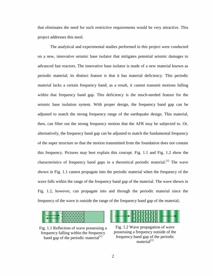
this frequency. Pictures may best explain this concept. Fig. 1.1 and Fig. 1.2 show the
characteristics of frequency band gaps in a theoretical periodic material.[1]
The wave
shown in Fig. 1.1 cannot propagate into the periodic material when the frequency of the
wave falls within the range of the frequency band gap of the material. The wave shown in
Fig. 1.2, however, can propagate into and through the periodic material since the
frequency of the wave is outside the range of the frequency band gap of the material;
Fig. 1.1 Reflection of wave possessing a
frequency falling within the frequency
band gap of the periodic material[1]
Fig. 1.2 Wave propagation of wave
possessing a frequency outside of the
frequency band gap of the periodic
material[1]
3
this periodic material-based method manipulates or blocks seismic wave energies in
isolation system. In other words, the materials and isolation systems, properly designed
and constructed, will possess frequency band gaps that will alter or block the energy
input without the undesirable effects of more traditional base isolation systems such as
residual displacements between the foundation and the supported structure.
The band gap phenomenon of periodic material has been known since 1900; the
theory was established in 1920. The major applications for this material have been in
solid-state physics. Recently, this material was proposed for seismic isolation used in
civil structures; if this innovative idea is applied to civil structures, the impact on the
economy and safety could be enormous.
1.2 Objective of Report
The goal of the proposed research is to develop a base isolation system that uses
periodic materials to obstruct completely or change the pattern of earthquake event
energy before it reaches the foundation of structural systems in nuclear power plants.
This goal reached would result in total isolation of the foundation from earthquake wave
energy, because no energy would be passing through it. Total isolation would be of
special significance to structures in nuclear power plants.
This project implemented an experimental program to verify and refine the
analytical study results and the basic design parameters. The project also generated
information needed to quantify the behavior of various periodic materials and material
combinations when they are used in standard nuclear containment configurations and
practices. The one-dimensional (1D) layered periodic foundation shake table test was
conducted; two-dimensional (2D) and three-dimensional (3D) periodic foundations were
4
tested in the free field by using the truck-mounted dynamic load generators. The test
results were used to verify and refine the design theory and procedures of periodic
material-based seismic isolation systems.
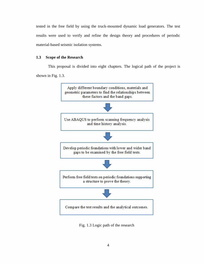
1.3 Scope of the Research
This proposal is divided into eight chapters. The logical path of the project is
shown in Fig. 1.3.
Fig. 1.3 Logic path of the research
5
Chapter 1 shows significance and objective of the research and presents the
outline of the report.
Chapter 2 describes a literature study of the past relevant work in the base
isolation system. Then, the background of phononic crystals is introduced since the basic
idea of periodic foundations is delivered from the concept of phononic crystals. Finally,
recent studies of periodic structures are introduced.
Chapter 3 presents the basic theory of periodic foundations. Next, theoretical
solutions of frequency band gaps are obtained for the 1D, 2D, and 3D periodic
foundations.
Chapter 4 discusses the attenuation zones of the periodic foundations given by
using the finite element method (FEM). The parametric studies are conducted first for
1D, 2D, and 3D periodic foundations. Then, scanning frequency analysis is performed
with both shear wave (S wave) and primary wave (P wave) excitations to obtain
attenuation zones for 1D, 2D, and 3D periodic foundations.
Chapter 5 describes experimental programs according to the FEM results (in
Chapter 4), specimens of periodic foundations are designed, and the test setup is
described.
Chapter 6 presents the test results under different dynamic loads, i.e., stepped sine
waves, fixed sine waves, and seismic waves for both S and P waves.
Chapter 7 shows the comparison of test results for 1D, 2D, and 3D periodic
foundations and the finite element analysis (FEA) outcomes in both time domain and
frequency domain.
Chapter 8 presents conclusions and suggests further studies in this area.

6
7
2 LITERATURE REVIEW
2.1 Overview of Base Isolation Systems
The design of buildings and other structures capable of withstanding earthquake
events has been the focus of research by engineers for many decades. A commonly
accepted method for the design of seismic-resistant buildings and structures, however,
has not yet been developed. Traditional design methods based simply on static structural
strength with impact factors to account for dynamic loads, fortunately, have been
reviewed and gradually replaced by novel methodologies over the last three decades.
Evolving concepts of structural element ductility and the importance of shear resistance
have contributed to the effective design of structural elements and systems resistant to
dynamic loadings from earthquakes. Passive and active systems have been proposed and
implemented to augment the ability of the structure to resist an earthquake event.
2.1.1 The passive base isolation system
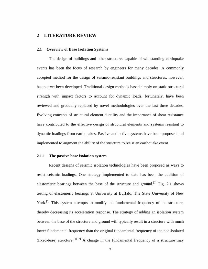
Recent designs of seismic isolation technologies have been proposed as ways to
resist seismic loadings. One strategy implemented to date has been the addition of
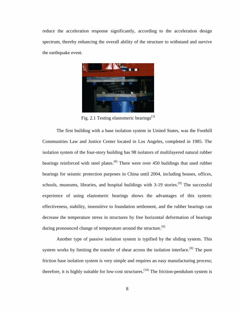
elastomeric bearings between the base of the structure and ground.[2]
Fig. 2.1 shows
testing of elastomeric bearings at University at Buffalo, The State University of New
York.[3]
This system attempts to modify the fundamental frequency of the structure,
thereby decreasing its acceleration response. The strategy of adding an isolation system
between the base of the structure and ground will typically result in a structure with much
lower fundamental frequency than the original fundamental frequency of the non-isolated
(fixed-base) structure.[4]-[7]
A change in the fundamental frequency of a structure may
8
reduce the acceleration response significantly, according to the acceleration design
spectrum, thereby enhancing the overall ability of the structure to withstand and survive
the earthquake event.
The first building with a base isolation system in United States, was the Foothill
Communities Law and Justice Center located in Los Angeles, completed in 1985. The
isolation system of the four-story building has 98 isolators of multilayered natural rubber
bearings reinforced with steel plates.[8]
There were over 450 buildings that used rubber
bearings for seismic protection purposes in China until 2004, including houses, offices,
schools, museums, libraries, and hospital buildings with 3-19 stories.[9]
The successful
experience of using elastomeric bearings shows the advantages of this system:
effectiveness, stability, insensitive to foundation settlement, and the rubber bearings can
decrease the temperature stress in structures by free horizontal deformation of bearings
during pronounced change of temperature around the structure.[9]
Another type of passive isolation system is typified by the sliding system. This
system works by limiting the transfer of shear across the isolation interface.[8]
The pure
friction base isolation system is very simple and requires an easy manufacturing process;
therefore, it is highly suitable for low-cost structures.[10]
The friction-pendulum system is
Fig. 2.1 Testing elastomeric bearings[3]
9
a sliding system using a special interfacial material sliding on stainless steel and has been
used for several projects in the United States, both in new and retrofitted constructions.[8]
Recently, more advanced techniques and materials have been added to sliding isolation
systems, including the Electricite De France (EDF) system, the Resilient Friction Base
Isolator (RFBI) system, the Sliding Resilient Friction (SRF), which combines the
desirable feature of EDF and RFBI system, TAISEI Shake Suppression (TASS) system,
the Friction Pendulum system (FPS), and the elliptical rolling rods.[11]
The Electricite De France (EDF) system is a friction-type base isolator consisting
of a laminated (steel-reinforced) neoprene pad topped by a lead-bronze plate, which is in
frictional contact with a steel plate anchored to the structure.[12]
The EDF system has
been used in a nuclear power plant at Koeberg in South Africa.
Mostaghel and Khodaverdian proposed the Resilient Friction Base Isolator
(RFBI) system in 1987. The RFBI system consists of a set of flat rings, which can slide
on each other and have a central rubber core and/or peripheral rubber cores. The RFBI
(isolator) combines friction damping and the resiliency of rubber.[13]
Su et al., presented a Sliding Resilient Friction (SRF) system in 1991.[14]
The SRF
system combines the advantages of EDF and RFBI base isolators. Absent large
displacements, using an SRF system can reduce a structure’s peak accelerations and
deflections; the system also provides additional safety against unexpected severe ground
motions.
The TAISEI Shake Suppression (TASS) system is composed of two types of
bearings, such as rubber bearings and sliding bearings.[15]
The TASS system was
developed for high-rise buildings.[16]
It was proved experimentally with high-strength
10
materials; and a long-span structure system would provide seismic isolation for high-rise
buildings undergoing strong ground motions.
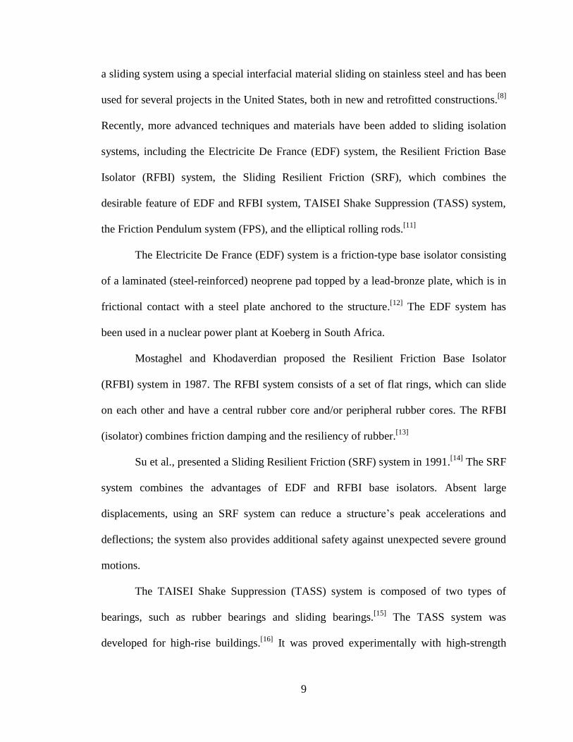
A friction pendulum system (FPS) is based on the principles of pendulum motion.
The friction damping absorbs the energy of the structure supported by FPS.[17]
Fig. 2.2
shows the friction pendulum-bearing used in the Benicia-Martinez Bridge Retrofit.[18]
The elliptical rolling rods overcome the disadvantages of circular rolling rods, i.e.,
large peak and residual base displacements. Elliptical rolling rods were effective in
reducing the seismic response of the system without undergoing large base
displacements.[19]
The roller bearings require maintenance throughout their working life,
however, and the system can isolate the ground motion in only one direction.
One significant drawback of a traditional seismic isolation system is that it will
usually have residual (permanent) horizontal displacements after earthquake events. The
bearings are very stiff in the vertical direction and are very flexible in the horizontal
direction. The action of the bearings under seismic loading is to isolate the building from
horizontal components of earthquake ground movement, while vertical components of
earthquake ground movement are transmitted through to the structure relatively
unchanged.
Fig. 2.2 Friction pendulum bearing used in Benicia-Martinez Bridge[18]

11
2.1.2 The active base isolation system
Active base isolation, which is composed of a passive isolation system combined
with control actuators, has been proposed as an alternative to overcome the disadvantages
of passive base isolation systems. In active isolation systems, the control actuators are
used to reduce drifts and floor accelerations. Many small-scale experiments of active base
isolation systems have been performed and the effectiveness of such systems proved.
Nagarajaiah et al.,[20]
presented an experimental and analytical study of hybrid
control of bridges using sliding bearings, with re-centering springs and servo-hydraulic
actuators; this study produced the control algorithm based on instantaneous optimal
control laws. The study showed that, with hybrid control, accelerations were reduced
substantially, while sliding displacement was confined within an acceptable range; post
earthquake permanent offsets were eliminated almost completely.
Schmitendorf et al.,[21]
presented an effective control technique for application to
seismic-excited building structures. The control method was robust with respect to
parameter uncertainty on the model, and it could easily incorporate actuator dynamics,
thus eliminating the adverse effects resulting from the slow response of the actuator.
Yang et al.,[22]
proposed robust control methods for seismic excited buildings
isolated by a frictional-type sliding-isolation system. A three-story quarter-scale
nonlinear building model was tested to verify the control methods. The building model
was mounted on a base-mate supported by four frictional bearings. Experimental test
results indicated that the control performance was remarkable, although a slight
degradation was observed owing to noise pollution and system time delays.
12
Chang and Spencer[23]
tested an active base isolation system with unique features
including low-friction pendular bearings and custom-manufactured low-force hydraulic
actuators. The control-structure interaction was also considered in these control
strategies, and the strategies were proved to perform effectively for a wide range of
seismic excitation.
As reported by Mehrparvar and Khoshnoudian,[24]
several advantages of active
control systems over passive devices can be cited, such as enhanced effectiveness in
response control, relative insensitivity to site conditions and ground motions,
applicability to multi-hazard mitigation situations, and selectivity of control objectives.
The active control system nevertheless requires a large external power supply for
structural systems during seismic events, which along with reliability and other issues,
make them unsuitable for broad application in civil engineering. In contrast, semi-active
control systems possess most of the advantages of active control systems without
requiring large energy sources; however, the semi-active control systems lack
reliability.[25]
Complex details and high costs, moreover, put a drag on their practical
application.
2.2 Overview of Phononic Crystals
The concept of phononic crystals is analogous to photonic crystals. Photonic
crystals are composed of periodic dielectric, metallo-dielectric, or even superconductor
microstructures or nanostructures that affect the propagation of electromagnetic waves
(EM); specific frequency ranges of EM are unable to pass through the photonic crystal;
these frequency ranges are called band gaps.
13
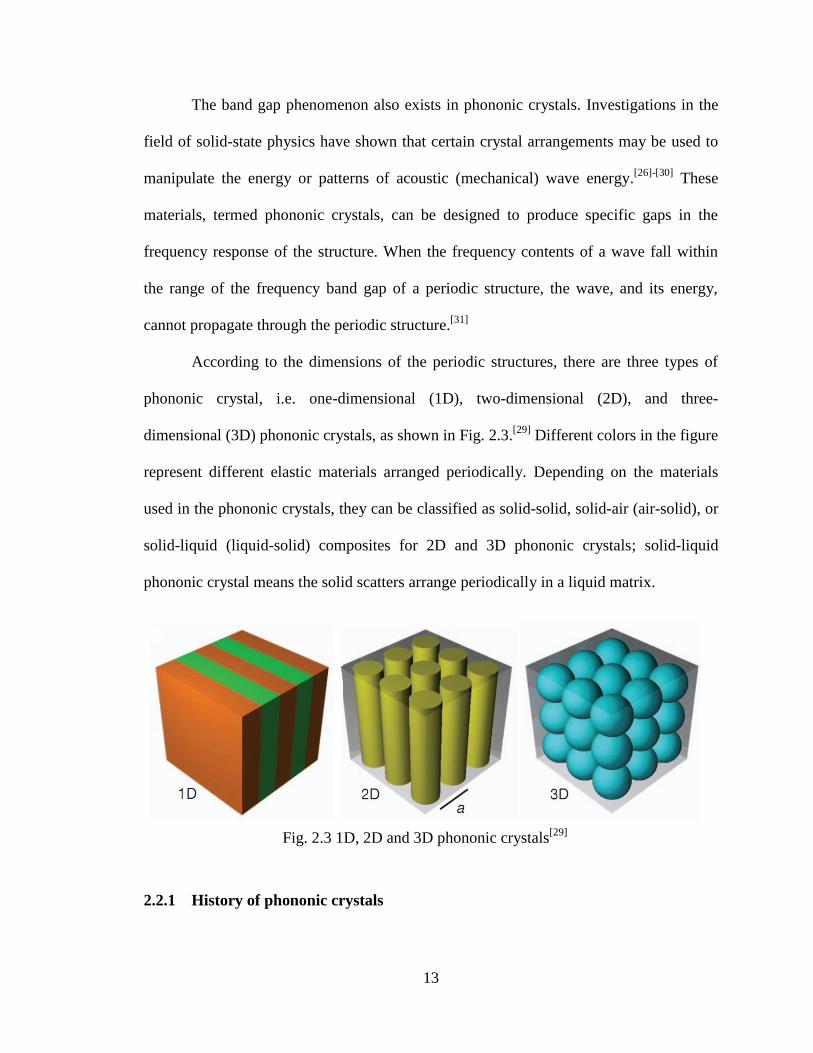
The band gap phenomenon also exists in phononic crystals. Investigations in the
field of solid-state physics have shown that certain crystal arrangements may be used to
manipulate the energy or patterns of acoustic (mechanical) wave energy.[26]-[30]
These
materials, termed phononic crystals, can be designed to produce specific gaps in the
frequency response of the structure. When the frequency contents of a wave fall within
the range of the frequency band gap of a periodic structure, the wave, and its energy,
cannot propagate through the periodic structure.[31]
According to the dimensions of the periodic structures, there are three types of
phononic crystal, i.e. one-dimensional (1D), two-dimensional (2D), and three-
dimensional (3D) phononic crystals, as shown in Fig. 2.3.[29]
Different colors in the figure
represent different elastic materials arranged periodically. Depending on the materials
used in the phononic crystals, they can be classified as solid-solid, solid-air (air-solid), or
solid-liquid (liquid-solid) composites for 2D and 3D phononic crystals; solid-liquid
phononic crystal means the solid scatters arrange periodically in a liquid matrix.
2.2.1 History of phononic crystals
Fig. 2.3 1D, 2D and 3D phononic crystals[29]
14
In 1992 for the first time, Sigalas and Economou[32]
proved theoretically the
existence of frequency band gaps of elastic and acoustic waves in periodic structures
consisting of identical spheres placed periodically within a homogeneous host material.
In 1993, Kushwaha et al.,[33]
obtained the band gaps of 2D phononic crystal using the
plane wave expansion method. They also pointed out that one can design the phononic
crystal to provide a vibrationless environment for high-precision mechanical systems in a
given frequency range.[34]
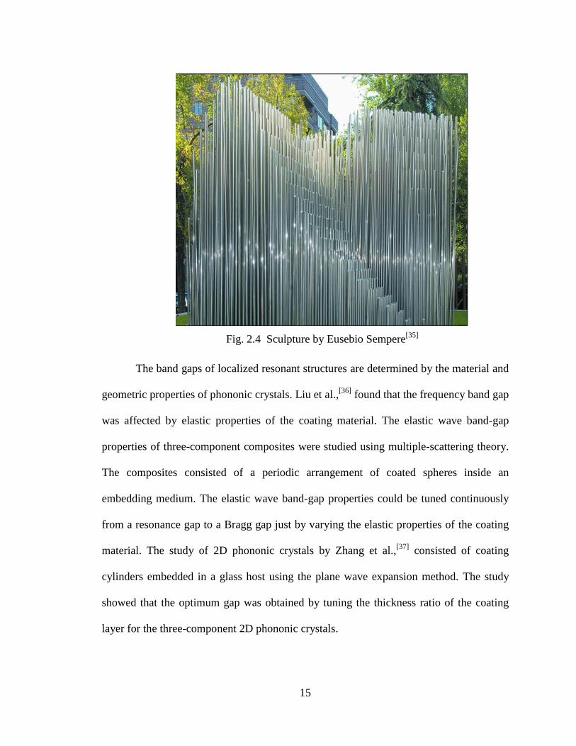
Eusebio Sempere’s kinematic sculpture as shown in Fig. 2.4, is
made of a periodic array of hollow stainless-steel cylinders of 2.9cm diameter, arranged
on a square 10×10cm lattice.[35]
In 1995, researchers at the Materials Science Institute of
Madrid showed that the sculpture strongly attenuated sound waves at certain frequencies,
thus providing the first experimental evidence for the existence of phononic band gaps in
periodic structures. In 2000, Liu and Zhang et al.,[27]
proposed the idea of localized
resonant structures, 3D periodic materials with lower frequency band gaps. The size of
the lattice constant is two orders of magnitude smaller than the wavelength of the band
gaps. The literature before 2000 showed that the wavelength of the band gaps had the
same size as the lattice constant due to Bragg scattering. The theory of localized resonant
structures may lead to applications in seismic wave reflection, since the frequency band
gaps can be reduced to very low ranges.
15
The band gaps of localized resonant structures are determined by the material and
geometric properties of phononic crystals. Liu et al.,[36]
found that the frequency band gap
was affected by elastic properties of the coating material. The elastic wave band-gap
properties of three-component composites were studied using multiple-scattering theory.
The composites consisted of a periodic arrangement of coated spheres inside an
embedding medium. The elastic wave band-gap properties could be tuned continuously
from a resonance gap to a Bragg gap just by varying the elastic properties of the coating
material. The study of 2D phononic crystals by Zhang et al.,[37]
consisted of coating
cylinders embedded in a glass host using the plane wave expansion method. The study
showed that the optimum gap was obtained by tuning the thickness ratio of the coating
layer for the three-component 2D phononic crystals.
Fig. 2.4 Sculpture by Eusebio Sempere[35]
16
Liu et al.,[38]
provided a simple analytic model for sonic band gaps owing to
resonance. In their paper, they described the origin of band gaps in the local resonant
phenomenon.
Goffaux et al.,[39]-[41]
studied elastic wave propagation in a locally resonant sonic
material. They introduced a simple mechanical model to show a physical insight of the
local resonance phenomenon. The researchers[41]
made a comparison of the Bragg gap
and resonance gap; the Bragg gap had even better attenuation performances on a larger
range of frequencies owing to Bragg interference phenomena at low frequencies.
Ho et al.,[42]
demonstrated a broadband sound shield based on layers of locally
resonant sonic materials. A broadband (200–500 Hz) sound barrier was achieved, and it
was significantly better than that dictated by mass density law.
Zhang and Cheng[43][44]
had already made a comparison of the band gaps between
the binary and three-component composite 2D phononic crystal, theoretically and
experimentally. Both results proved the existence of a much broader gap of the three-
component crystal slab over the binary.
Hirsekorn et al.,[45][46]
performed numerical simulations of acoustic wave
propagation through sonic crystals consisting of local resonators using the Local
Interaction Simulation Approach (LISA). Three strong attenuation bands were found at
frequencies between 0.3 and 6.0 kHz, which do not depend on the periodicity of the
crystal.
Wang et al.,[47][48]
studied the propagation of elastic waves in 2D binary phononic
crystals consisting of soft rubber cylinders in epoxy. The binary locally resonant
17
materials were studied using the lumped-mass method. The first and second in-plane
locally resonant modes were localized in both the coating layer and the core.
Hsu and Wu[49]
studied the 2D two-component phononic crystal plated with a
finite thickness using the plane wave expansion method. The low-frequency gaps of
Lamb waves owing to localized resonance mechanism and flexure-dominated plate
modes were significantly dependent, not only on the filling ratios, but also on the plate
thickness.
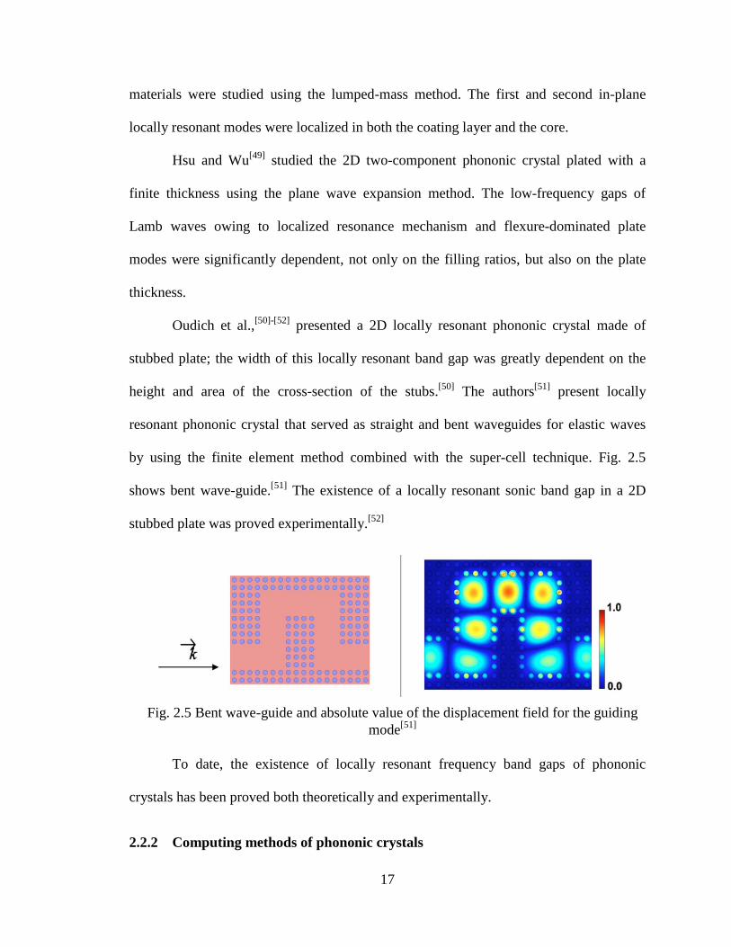
Oudich et al.,[50]-[52]
presented a 2D locally resonant phononic crystal made of
stubbed plate; the width of this locally resonant band gap was greatly dependent on the
height and area of the cross-section of the stubs.[50]
The authors[51]
present locally
resonant phononic crystal that served as straight and bent waveguides for elastic waves
by using the finite element method combined with the super-cell technique. Fig. 2.5
shows bent wave-guide.[51]
The existence of a locally resonant sonic band gap in a 2D
stubbed plate was proved experimentally.[52]
To date, the existence of locally resonant frequency band gaps of phononic
crystals has been proved both theoretically and experimentally.
2.2.2 Computing methods of phononic crystals
Fig. 2.5 Bent wave-guide and absolute value of the displacement field for the guiding
mode[51]
18
There are several ways to obtain frequency band gaps of phononic crystals. Five
of them are commonly used: (1) the transfer matrix method, (2) the plane wave expansion
method, (3) the finite different time domain method, (4) the multiple scattering theory,
and (5) the finite element method.
The transfer matrix (TM) method[53]-[57]
needs only a small amount of
computation, and it is used in 1D phononic crystals, i.e., phononic crystal Euler beams
and phononic crystal bars. Using the motion equations of the beams or bars, along with
the continuous conditions at the interface, i.e., the displacement, rotation angle, bending
moment, and shear force, the transfer matrix of the TM method can be obtained. One can
obtain an Eigen value problem with the transfer matrix and periodic boundary conditions,
which contain the dispersion relation of phononic crystals. The main advantage of the
TM method is that only a small amount of computation is needed. The TM method
cannot be used, however, to solve the band structures of 2D and 3D phononic crystals.
The plane wave expansion (PWE) method[32]-[34][39][58]-[61]
is one of the most
popular ways to obtain the band gaps of phononic crystals. Until now, the method has
been used to solve the band gaps of phononic crystals with solid-solid, solid-air (air-
solid), solid-liquid (liquid-solid) composites. Owing to the periodic boundary conditions
of phononic crystals, the densities and elastic constants of the materials can be written as
Fourier series expansions. Taken with the Bloch’s theorem, the equations of motion can
be written in the form of Eigen value equations, and the problem is converted to an Eigen
value problem. The PWE method encounters convergence problems when the phononic
crystal has a large elastic difference. The method becomes both time-consuming and
difficult in memory requirements with the increasing of the plane waves.
19
The finite difference time domain (FDTD) method[62]-[65]
is suitable for dealing
with different geometric structures and for handling the numerical convergence problem.
The wave equations are discretized in the time domain first, and the periodic boundary
conditions and the Bloch’s theorem are applied next. With a given excitation, the
response of phononic crystals in the time domain can be obtained. After the Fourier
Transform is applied, the Eigen values from the frequency spectrum can be obtained, and
the band gaps of the phononic crystals solved. The FDTD method requires considerable
calculation; therefore, parallel computing technology and high efficiency computers are
needed.
Multiple scattering theory (MST)[66]-[69]
can be used for 2D and 3D phononic
crystals; MST is an exact theory without approximation; however, it is suitable only for
highly symmetric scatters of 2D and 3D phononic crystals.
The finite element (FE) method is a numerical technique for finding approximate
solutions to boundary value problems for differential equations. To obtain the band gaps
of phononic crystals, the periodic boundary conditions are applied to the unit cells.
Commercial software such as ABAQUS and ANSYS cannot be used to apply the
periodic boundary conditions to the phononic crystals directly. COMSOL Multiphysics,
however, provides periodic boundary conditions that can be used very easily.
2.2.3 Application of phononic crystals
Kushwaha[34]
proposed for the first time in 1993 the idea that phononic crystals
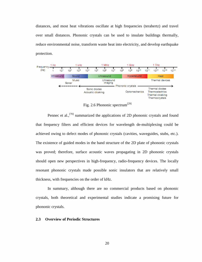
can be used for vibrationless environments. Maldovan[29]
summarized the frequency
ranges in which phononic crystals would work and their possible applications, as shown
in Fig. 2.6. Sound waves oscillate at low frequencies (kilohertz) and propagate over large
20
distances, and most heat vibrations oscillate at high frequencies (terahertz) and travel
over small distances. Phononic crystals can be used to insulate buildings thermally,
reduce environmental noise, transform waste heat into electricity, and develop earthquake
protection.
Pennec et al.,[70]
summarized the applications of 2D phononic crystals and found
that frequency filters and efficient devices for wavelength de-multiplexing could be
achieved owing to defect modes of phononic crystals (cavities, waveguides, stubs, etc.).
The existence of guided modes in the band structure of the 2D plate of phononic crystals
was proved; therefore, surface acoustic waves propagating in 2D phononic crystals
should open new perspectives in high-frequency, radio-frequency devices. The locally
resonant phononic crystals made possible sonic insulators that are relatively small
thickness, with frequencies on the order of kHz.
In summary, although there are no commercial products based on phononic
crystals, both theoretical and experimental studies indicate a promising future for
phononic crystals.
2.3 Overview of Periodic Structures
Fig. 2.6 Phononic spectrum[29]
21
Guided by recent advances in solid-state research and the concept of frequency
band gaps in periodic materials such as phononic crystals, this new periodic material is
used in seismic base isolation as an innovative means to mitigate potential damage to
structures. With this periodic material, the pattern of the earthquake event energy will be
completely obstructed or changed when it reaches the periodic foundation of the
structural system; this will result in a total isolation of the foundation from the earthquake
wave energy because no energy will pass through it. The upper structure, therefore, can
be protected during an earthquake along with non-structural components. This total
isolation will be of special significance to some specific structures housing highly
vibration-sensitive equipment such as research laboratories, medical facilities with
sensitive imaging equipment, or high-precision facilities specializing in the fabrication of
electronic components. Further, the full isolation of emergency-critical structures such as
bridges, hospitals housing emergency response units or equipment, and power generation
or distribution structures will have a better earthquake emergency response;
consequently, there will be fewer compromises to the entire emergency response system.
Periodic foundations are arranged in a periodic way in one, two, and three directions,
which are defined in Fig. 2.7 as one-dimensional periodic foundation (1D), two-
dimensional periodic foundation (2D), and three-dimensional periodic foundation (3D),
respectively. The frequency band gaps of the periodic foundations are also called
attenuation zones. Many studies have been conducted to investigate the 1D layered
periodic structures both theoretically and experimentally.
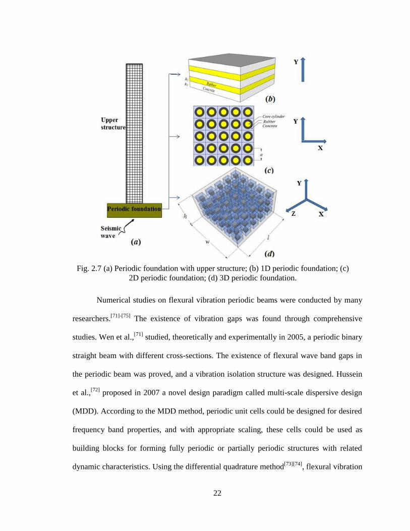
22
Numerical studies on flexural vibration periodic beams were conducted by many
researchers.[71]-[75]
The existence of vibration gaps was found through comprehensive
studies. Wen et al.,[71]
studied, theoretically and experimentally in 2005, a periodic binary
straight beam with different cross-sections. The existence of flexural wave band gaps in
the periodic beam was proved, and a vibration isolation structure was designed. Hussein
et al.,[72]
proposed in 2007 a novel design paradigm called multi-scale dispersive design
(MDD). According to the MDD method, periodic unit cells could be designed for desired
frequency band properties, and with appropriate scaling, these cells could be used as
building blocks for forming fully periodic or partially periodic structures with related
dynamic characteristics. Using the differential quadrature method[73][74]
, flexural vibration
Fig. 2.7 (a) Periodic foundation with upper structure; (b) 1D periodic foundation; (c)
2D periodic foundation; (d) 3D periodic foundation.
23
band gaps in periodic beams were studied, considering the influences of shear
deformation, geometrical parameters, and material parameters. Attenuation in band gaps
delivered a new idea in structural design to weaken vibration. The critical frequency was
found, owing to the Pasternak foundation, and a comprehensive parameter study was
conducted to highlight the influence of the foundation modulus on the band gaps. Yu et
al., [75]
found that, by analyzing the beam on elastic foundations using the transfer matrix
method, a gap with low frequency and wide range could exist in a beam on elastic
foundations.
The 1D periodic structure was used as the legs of an offshore platform, as shown
in Fig. 2.8.[76][77]
The periodic legs were discussed theoretically using the transfer matrix
method and validated experimentally using a scaled experimental model of an offshore
platform. Periodic legs were found to isolate the vibration transmitted from sea waves to
offshore platform structures in the axial and lateral directions over a broad frequency
band.
The 1D periodic structures were used as foundations and to isolate upper
structures.[78]-[80]
The 1D layered periodic foundation is discussed theoretically.[78]
Studies
Fig. 2.8 Oil and gas offshore platform
24
of dynamic responses of a seven-story frame structure with three different foundations
were conducted and compared to test the validity of the periodic isolated foundation. A
1D periodic structure, it was found, was an effective method to block seismic waves for
structures in civil engineering. Shi et al.,[79]
proposed a new type of a seismic isolation
foundation configuration containing several concrete layers and rubber blocks. The
equivalent analytical model for the periodic foundation and two formulas were
established. The first attenuation zone of the new configuration of a seismic isolation
foundation was as low 2.15 Hz to 15.01 Hz for seismic protection. Cheng and Shi[80]
proposed a multi-mass-spring model to study the band of frequency gaps of 1D periodic
structures, and they investigated the dynamic properties of finite periodic structures from
an energy viewpoint.
The existence of frequency band gaps of a 2D periodic structure has been studied
theoretically and experimentally. [81]-[86]
Two-dimensional periodic foundations have been
studied theoretically[81]-[84]
; the 2D periodic foundation with a low frequency gap was
achieved. Simulations demonstrated that periodic foundations could greatly reduce the
dynamic response of upper structures under both vertical and longitudinal ground
motions. Two-dimensional periodic structures were used as pile barriers owing to the
frequency band gap effect of the periodic structure.[85]
The periodic pile barrier
significantly reduced the vibration in the frequency band gaps. A large-scale experiment,
as shown in Fig. 2.9, was performed.[86]
The test showed that a structured soil consisting
of clay with 5-m deep boreholes shielded surface elastic waves of around 50 Hz. Then,
numerical simulations were conducted to simulate the energy field, and they were
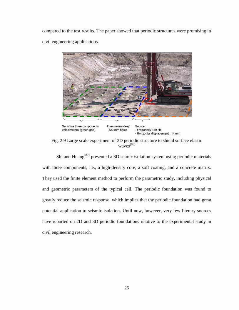
25
compared to the test results. The paper showed that periodic structures were promising in
civil engineering applications.
Shi and Huang[87]
presented a 3D seimic isolation system using periodic materials
with three components, i.e., a high-density core, a soft coating, and a concrete matrix.
They used the finite element method to perform the parametric study, including physical
and geometric parameters of the typical cell. The periodic foundation was found to
greatly reduce the seismic response, which implies that the periodic foundation had great
potential application to seismic isolation. Until now, however, very few literary sources
have reported on 2D and 3D periodic foundations relative to the experimental study in
civil engineering research.
Fig. 2.9 Large scale experiment of 2D periodic structure to shield surface elastic
waves[86]

27
3 THE BASIC THEORIES OF PERIODIC FOUNDATIONS
The basic theories of periodic structures composed of infinite unit cells are
illustrated in this chapter. The transfer matrix method, plane wave expansion method, and
finite difference time domain method for 1D, 2D, and 3D periodic foundations are
introduced in detail; the frequency band gaps of periodic foundations with infinite unit
cells are calculated.
3.1 Basic Theories of 1D Layered Periodic Foundations
The transfer matrix method of 1D periodic foundation band gaps was used to
solve the wave equations. Xiang et al.,[88]
illustrated a method to solve the 1D layered
periodic foundation. Fig. 3.1a. shows the 1D layered periodic material composed of two
materials, A and B; Fig. 3.1b. shows one unit cell of the 1D layered periodic foundation.
Each layer is extended infinitely in the XY plan, and the unit cells are repeated in the Z
direction infinitely for the coordinate system specified. The thickness of layer A and layer
B of a unit cell is h1 and h2, respectively. The periodicity of the foundation structure and
displacement makes it possible to investigate the frequency band gap by studying one
unit cell.
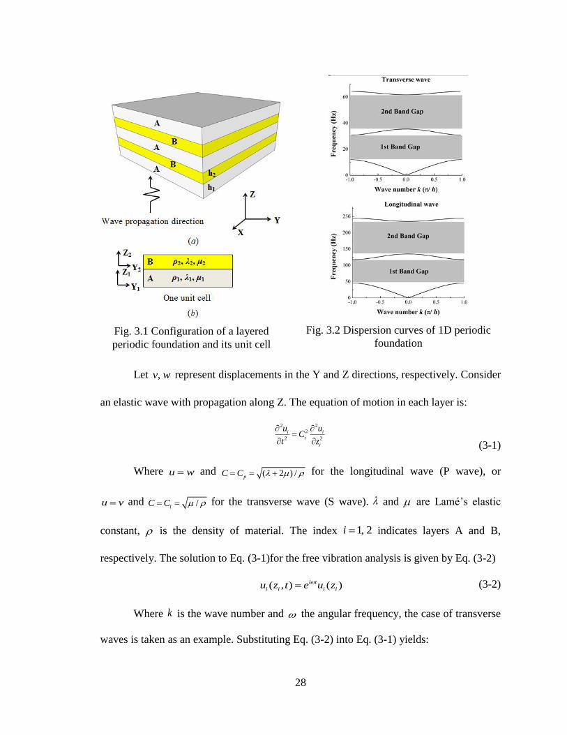
28
Let represent displacements in the Y and Z directions, respectively. Consider
an elastic wave with propagation along Z. The equation of motion in each layer is:
(3-1)
Where and for the longitudinal wave (P wave), or
and for the transverse wave (S wave). and are Lamé’s elastic
constant, is the density of material. The index indicates layers A and B,
respectively. The solution to Eq. (3-1)for the free vibration analysis is given by Eq. (3-2)
(3-2)
Where is the wave number and the angular frequency, the case of transverse
waves is taken as an example. Substituting Eq. (3-2) into Eq. (3-1) yields:
,v w
2 22
2 2
i ii
i
u uC
t z
u w ( 2 ) /pC C
u v /tC C
1, 2i
( , ) ( )i t
i i i iu z t e u z
k
Fig. 3.1 Configuration of a layered
periodic foundation and its unit cell
Fig. 3.2 Dispersion curves of 1D periodic
foundation
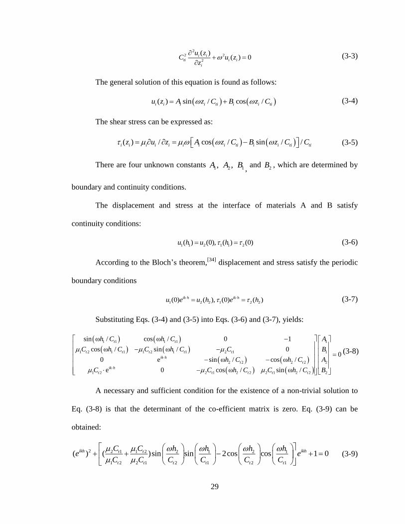
29
(3-3)
The general solution of this equation is found as follows:
(3-4)
The shear stress can be expressed as:
(3-5)
There are four unknown constants , and , which are determined by
boundary and continuity conditions.
The displacement and stress at the interface of materials A and B satisfy
continuity conditions:
(3-6)
According to the Bloch’s theorem,[34]
displacement and stress satisfy the periodic
boundary conditions
(3-7)
Substituting Eqs. (3-4) and (3-5) into Eqs. (3-6) and (3-7), yields:
(3-8)
A necessary and sufficient condition for the existence of a non-trivial solution to
Eq. (3-8) is that the determinant of the co-efficient matrix is zero. Eq. (3-9) can be
obtained:
(3-9)
22 2
2
( )( ) 0i i
ti i i
i
u zC u z
z
( ) sin / cos /i i i i ti i i tiu z A z C B z C
( ) / cos / sin / /i i i i i i i ti i i t ti i iz u z A z C B z C C
1 2 1, ,A A B 2B
1 1 2 1 1 2( ) (0), ( ) (0)u h u h
1 2 2 1 2 2(0) ( ), (0) ( )ik h ik hu e u h e h
1 1 1 1 1
1 2 1 1 1 2 1 1 2 1 1
2 2 2 2 2
1 2 2 1 2 2 2 1 2 2 2
sin ω / cos ω / 0 1
cos ω / sin ω / 00
0 e sin ω / cos ω /
e 0 cos ω / sin ω /
t t
t t t t t
ik h
t t
ik h
t t t t t
h C h C A
C h C C h C C B
h C h C A
C C h C C h C B
2 1 12 2 1 22
1 2
1
2 12 11 2
( ) ( )sin sin 2cos cos 1 0ikh ikh
t t
t t
t t tt
h h h he e
C C C C
C C
C C
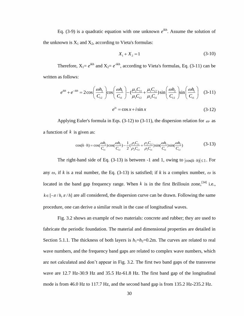
30
Eq. (3-9) is a quadratic equation with one unknown eikh
. Assume the solution of
the unknown is X1 and X2, according to Vieta's formulas:
(3-10)
Therefore, X1= eikh
and X2= e-ikh
, according to Vieta's formulas, Eq. (3-11) can be
written as follows:
(3-11)
(3-12)
Applying Euler's formula in Eqs. (3-12) to (3-11), the dispersion relation for as
a function of is given as:
(3-13)
The right-hand side of Eq. (3-13) is between -1 and 1, owing to . For
any ω, if k is a real number, the Eq. (3-13) is satisfied; if k is a complex number, ω is
located in the band gap frequency range. When is in the first Brillouin zone,[34]
i.e.,
are all considered, the dispersion curve can be drawn. Following the same
procedure, one can derive a similar result in the case of longitudinal waves.
Fig. 3.2 shows an example of two materials: concrete and rubber; they are used to
fabricate the periodic foundation. The material and dimensional properties are detailed in
Section 5.1.1. The thickness of both layers is h1=h2=0.2m. The curves are related to real
wave numbers, and the frequency band gaps are related to complex wave numbers, which
are not calculated and don’t appear in Fig. 3.2. The first two band gaps of the transverse
wave are 12.7 Hz-30.9 Hz and 35.5 Hz-61.8 Hz. The first band gap of the longitudinal
mode is from 46.0 Hz to 117.7 Hz, and the second band gap is from 135.2 Hz-235.2 Hz.
1 2 1X X
2 12 1 2 11 2
1 2 2 12 1 2 1
2cos cos ( )sin sinikh ikh
t t t
t
t t
t
t
h h h hC C
C Ce e
C C C C
cos sinixe x i x
k
1 1 2 21 2 1 2
1 2 2 2 1 1 1 2
1cos( ) cos( )cos( ) ( )sin( )sin( )
2
t t
t t t t t t
C Ch h h hk h
C C C C C C
1cos( )k h
k
[ / , / ]k h h
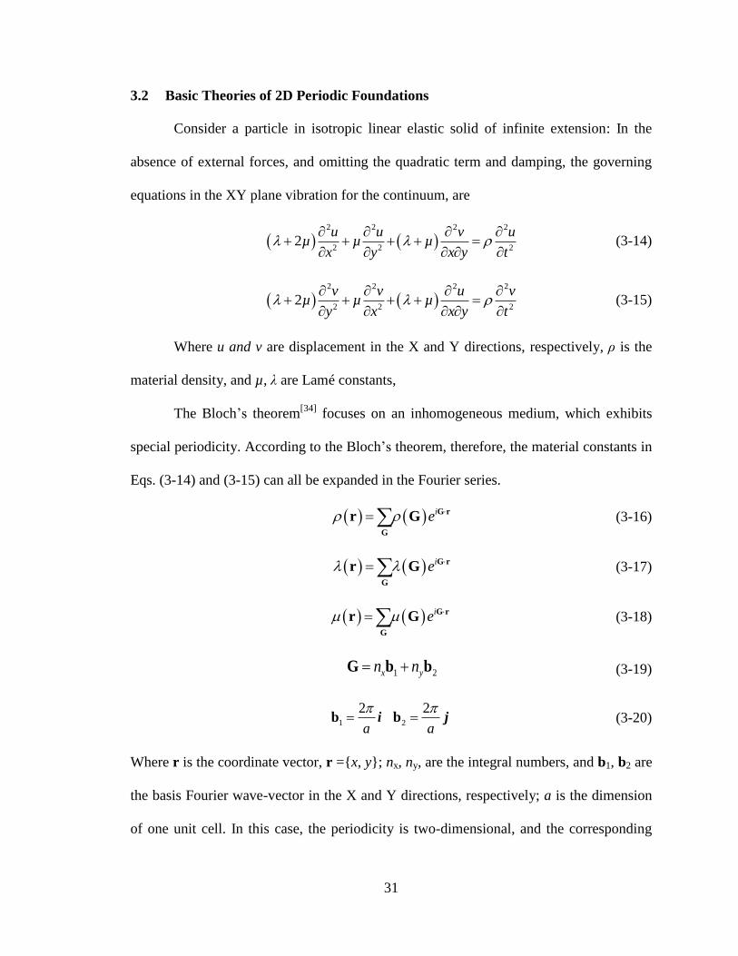
31
3.2 Basic Theories of 2D Periodic Foundations
Consider a particle in isotropic linear elastic solid of infinite extension: In the
absence of external forces, and omitting the quadratic term and damping, the governing
equations in the XY plane vibration for the continuum, are
(3-14)
(3-15)
Where u and v are displacement in the X and Y directions, respectively, ρ is the
material density, and µ, λ are Lamé constants,
The Bloch’s theorem[34]
focuses on an inhomogeneous medium, which exhibits
special periodicity. According to the Bloch’s theorem, therefore, the material constants in
Eqs. (3-14) and (3-15) can all be expanded in the Fourier series.
(3-16)
(3-17)
(3-18)
(3-19)
(3-20)
Where r is the coordinate vector, r ={x, y}; nx, ny, are the integral numbers, and b1, b2 are
the basis Fourier wave-vector in the X and Y directions, respectively; a is the dimension
of one unit cell. In this case, the periodicity is two-dimensional, and the corresponding
2 2 2 2
2 2 22
u u v uµ µ µ
x y x y t
2 2 2 2
2 2 22
v v u vµ µ µ
y x x y t
ie G r
G
r G
ie G r
G
r G
ie G r
G
r G
1 2x yn n G b b
1
2
a
b i 2
2
a
b j

32
reciprocal-lattice vector G has the same dimensionality. According to Eqs. (3-16) to (3-
18), the material properties in Eqs. (3-14) and (3-15) can be written as periodic functions
in periodic materials; Eqs. (3-16) to (3-18) sum up all the Fourier wave-vectors. The
displacement u(r), therefore, can be expressed as:
(3-21)
Where k is the Bloch wave vector and ω is the circular frequency of the wave. The plane
wave expansion method is illustrated as an example solution to the equations.
A square lattice periodic plate with three components is shown in Fig. 3.3; A, B,
and C are three different components. In this model, it is assumed that the plate only
deforms in the X-Y plane and that bending deformation is ignored.
According to the boundary conditions of a thin plate, the stress and strain
relationships can be obtained[89]
as follows:
(3-22)
,i t it e e
k r G r
k
G
u r u G
21xx
E u v
x y
Fig. 3.3 A three-components square lattice periodic structure
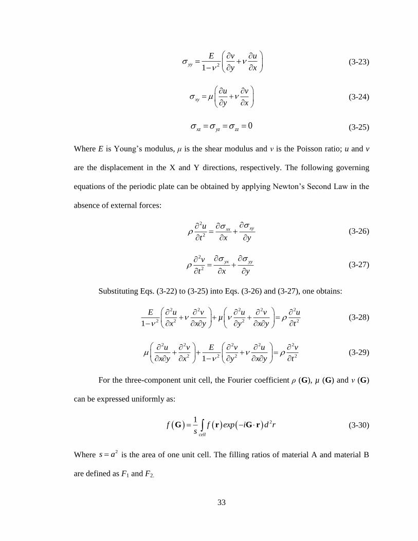
33
(3-23)
(3-24)
(3-25)
Where E is Young’s modulus, μ is the shear modulus and ν is the Poisson ratio; u and v
are the displacement in the X and Y directions, respectively. The following governing
equations of the periodic plate can be obtained by applying Newton’s Second Law in the
absence of external forces:
(3-26)
(3-27)
Substituting Eqs. (3-22) to (3-25) into Eqs. (3-26) and (3-27), one obtains:
(3-28)
(3-29)
For the three-component unit cell, the Fourier coefficient ρ (G), µ (G) and ν (G)
can be expressed uniformly as:
(3-30)
Where is the area of one unit cell. The filling ratios of material A and material B
are defined as F1 and F2.
21yy
E v u
y x
xy
u v
y x
0xz yz zz
2
2
xyxxu
t x y
2
2
yx yyv
t x y
2 2 2 2 2
2 2 2 21
E u v u v uµ
x x y y x y t
2 2 2 2 2
2 2 2 21
u v E v u v
x y x y x y t
21
cell
f f exp i d rs
G r G r
2s a
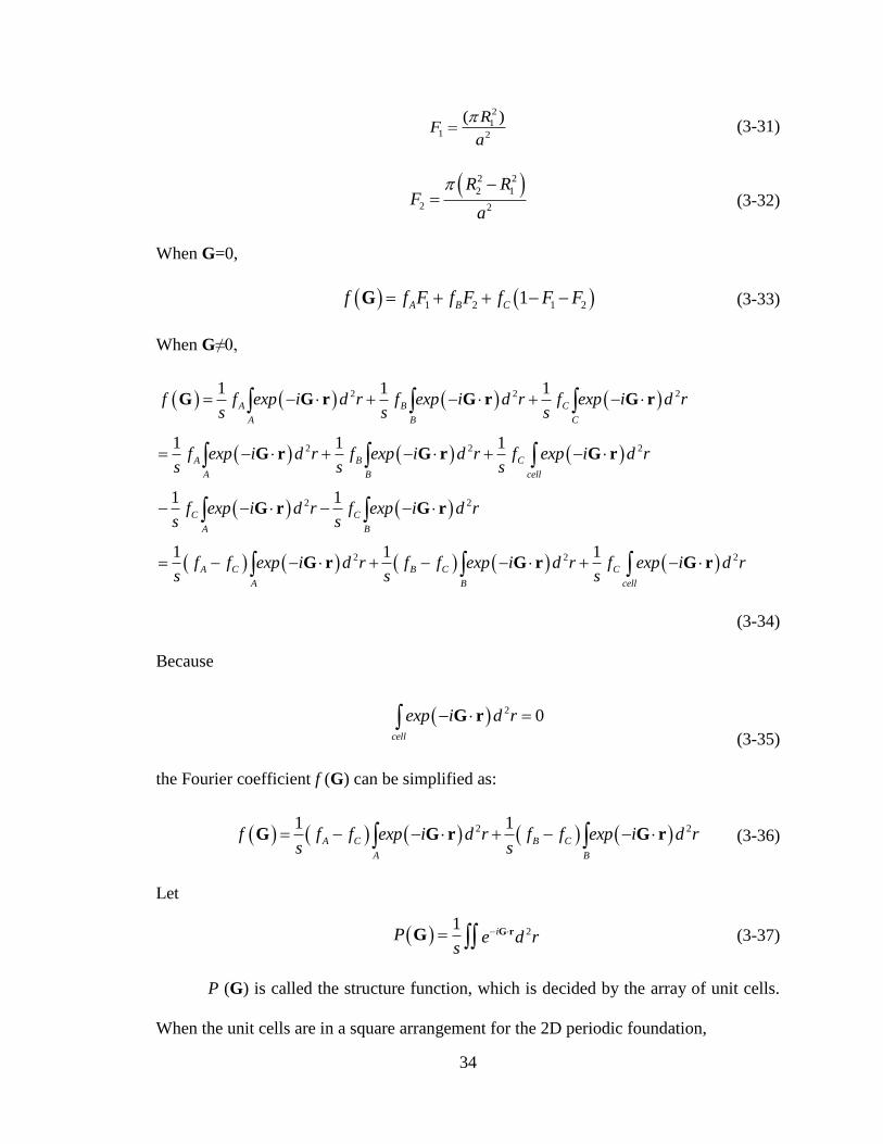
34
(3-31)
(3-32)
When G=0,
(3-33)
When G≠0,
(3-34)
Because
(3-35)
the Fourier coefficient f (G) can be simplified as:
(3-36)
Let
(3-37)
P (G) is called the structure function, which is decided by the array of unit cells.
When the unit cells are in a square arrangement for the 2D periodic foundation,
2
11 2
( )RF
a
2 2
2 1
2 2
R RF
a
1 2 1 21A B Cf f F f F f F F G
2 2 2
2 2 2
2 2
2 2
1 1 1
1 1 1
1 1
1 1 1
A B C
A B C
A B C
A B cell
C C
A B
A C B C C
A B cell
f f exp i d r f exp i d r f exp i d rs s s
f exp i d r f exp i d r f exp i d rs s s
f exp i d r f exp i d rs s
f f exp i d r f f exp i d r fs s s
G G r G r G r
G r G r G r
G r G r
G r G r 2exp i d r G r
2 0cell
exp i d r G r
2 21 1A C B C
A B
f f f exp i d r f f exp i d rs s
G G r G r
21
iP e d rs
G rG
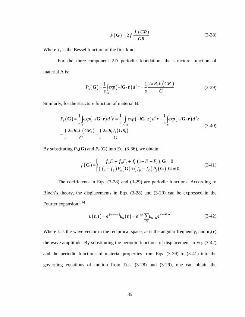
35
(3-38)
Where J1 is the Bessel function of the first kind.
For the three-component 2D periodic foundation, the structure function of
material A is:
(3-39)
Similarly, for the structure function of material B:
(3-40)
By substituting PA(G) and PB(G) into Eq. (3-36), we obtain:
(3-41)
The coefficients in Eqs. (3-28) and (3-29) are periodic functions. According to
Bloch’s theory, the displacements in Eqs. (3-28) and (3-29) can be expressed in the
Fourier expansion:[66]
(3-42)
Where k is the wave vector in the reciprocal space, ω is the angular frequency, and uk(r)
the wave amplitude. By substituting the periodic functions of displacement in Eq. (3-42)
and the periodic functions of material properties from Eqs. (3-39) to (3-41) into the
governing equations of motion from Eqs. (3-28) and (3-29), one can obtain the
1
2J GR
P fGR
G
1 1 12
21 1A
A
R J GRP exp i d r
s s G
G G r
2 2 2
2 1 2 1 1 1
1 1 1
2 21 1
B
B A B B
P exp i d r exp i d r exp i d rs s s
R J GR R J GR
s G s G
G G r G r G r
1 2 1 21 , 0
, 0
A B C
A B A B C B
f F f F f F Ff
f f P f f P
GG
G G G
,
i t ii tu t e u e u e
k r k G r
k k G
G
r r
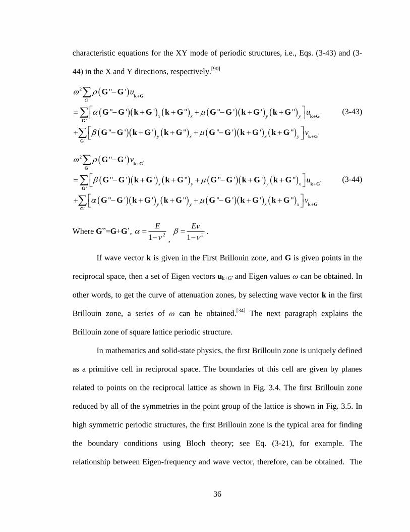
36
characteristic equations for the XY mode of periodic structures, i.e., Eqs. (3-43) and (3-
44) in the X and Y directions, respectively.[90]
(3-43)
(3-44)
Where G”=G+G’, ,
.
If wave vector k is given in the First Brillouin zone, and G is given points in the
reciprocal space, then a set of Eigen vectors uk+G’ and Eigen values ω can be obtained. In
other words, to get the curve of attenuation zones, by selecting wave vector k in the first
Brillouin zone, a series of ω can be obtained.[34]
The next paragraph explains the
Brillouin zone of square lattice periodic structure.
In mathematics and solid-state physics, the first Brillouin zone is uniquely defined
as a primitive cell in reciprocal space. The boundaries of this cell are given by planes
related to points on the reciprocal lattice as shown in Fig. 3.4. The first Brillouin zone
reduced by all of the symmetries in the point group of the lattice is shown in Fig. 3.5. In
high symmetric periodic structures, the first Brillouin zone is the typical area for finding
the boundary conditions using Bloch theory; see Eq. (3-21), for example. The
relationship between Eigen-frequency and wave vector, therefore, can be obtained. The
'
'
'
2
'
'
'
" '
" ' ' " " ' ' "
" ' ' " '' ' ' "
G
x x y y
y x x y
u
u
v
k G
k GG
k GG
G G
G G k G k G G G k G k G
G G k G k G G G k G k G
'
'
'
2
'
'
'
" '
" ' ' " " ' ' "
" ' ' " '' ' ' "
x y y x
y y x x
v
u
v
k GG
k GG
k GG
G G
G G k G k G G G k G k G
G G k G k G G G k G k G
21
E
21
E
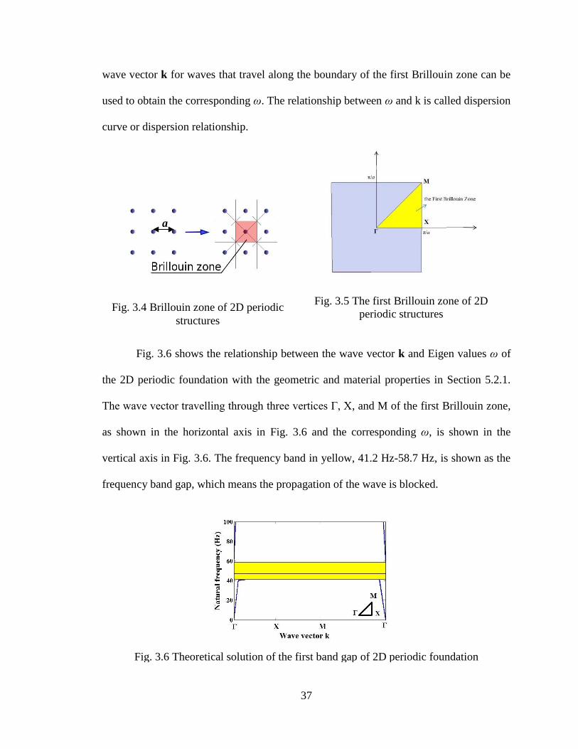
37
wave vector k for waves that travel along the boundary of the first Brillouin zone can be
used to obtain the corresponding ω. The relationship between ω and k is called dispersion
curve or dispersion relationship.
Fig. 3.6 shows the relationship between the wave vector k and Eigen values ω of
the 2D periodic foundation with the geometric and material properties in Section 5.2.1.
The wave vector travelling through three vertices Γ, X, and M of the first Brillouin zone,
as shown in the horizontal axis in Fig. 3.6 and the corresponding ω, is shown in the
vertical axis in Fig. 3.6. The frequency band in yellow, 41.2 Hz-58.7 Hz, is shown as the
frequency band gap, which means the propagation of the wave is blocked.
Fig. 3.4 Brillouin zone of 2D periodic
structures
Fig. 3.5 The first Brillouin zone of 2D
periodic structures
Fig. 3.6 Theoretical solution of the first band gap of 2D periodic foundation
a
38
3.3 Basic Theory of 3D Periodic Foundations
In the phononic crystal, many 3D structures are reported including simple cubic
(SC), body-centered cubic (BCC), and face-centered cubic (FCC).[91]-[94]
The PWE
method is used for 2D periodic structure analysis. The multiple scattering theory (MST)
is also used in 3D periodic acoustic composites and the band structures of a phononic
crystal consisting of complex and frequency-dependent Lamé coefficients.[66]-[69]
The
MST method, however, is only used for sphere scatters of 3D periodic structures and
cylinder scatters for 2D periodic structures; the PWE method encounters convergence
problems when the composites of the phononic crystal show a great difference in
Young’s modulus. The finite difference time domain (FDTD) method is suitable for
handling different geometric structures and the convergence problem, but it requires
considerable calculation.[63]
3.3.1 Basic equations of elastic wave
Three basic equations can be written for linear elastic isotropic material:
(1) Differential equation of motion;
(3-45)
(2) Equation of compatibility;
(3-46)
(3) Constitutive law.
or
(3-47)
,ij j i if u
2ij j i i ju u
2ij kk ij ij 1ij ij kk ij E
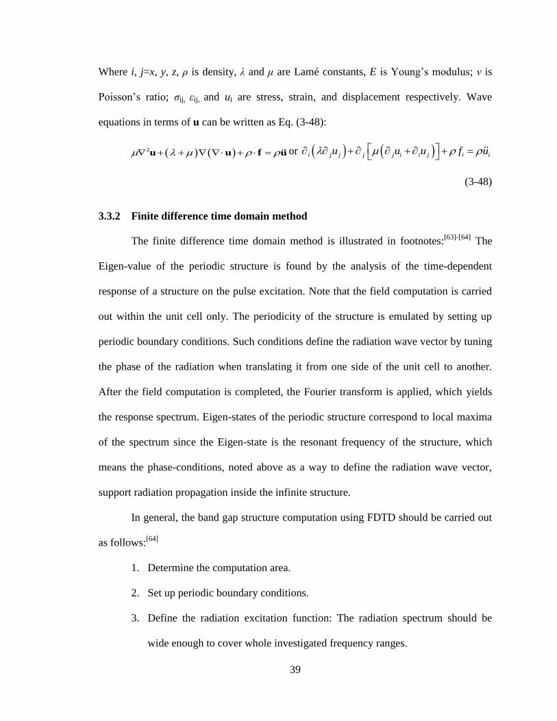
39
Where i, j=x, y, z, ρ is density, λ and μ are Lamé constants, E is Young’s modulus; ν is
Poisson’s ratio; σij, εij, and ui are stress, strain, and displacement respectively. Wave
equations in terms of u can be written as Eq. (3-48):
or
(3-48)
3.3.2 Finite difference time domain method
The finite difference time domain method is illustrated in footnotes:[63]-[64]
The
Eigen-value of the periodic structure is found by the analysis of the time-dependent
response of a structure on the pulse excitation. Note that the field computation is carried
out within the unit cell only. The periodicity of the structure is emulated by setting up
periodic boundary conditions. Such conditions define the radiation wave vector by tuning
the phase of the radiation when translating it from one side of the unit cell to another.
After the field computation is completed, the Fourier transform is applied, which yields
the response spectrum. Eigen-states of the periodic structure correspond to local maxima
of the spectrum since the Eigen-state is the resonant frequency of the structure, which
means the phase-conditions, noted above as a way to define the radiation wave vector,
support radiation propagation inside the infinite structure.
In general, the band gap structure computation using FDTD should be carried out
as follows:[64]
1. Determine the computation area.
2. Set up periodic boundary conditions.
3. Define the radiation excitation function: The radiation spectrum should be
wide enough to cover whole investigated frequency ranges.
2 u u f u i j j j j i i j i iu u u f u
40
4. Carry out spectral analysis of the time-dependent response of the structure on
the probe pulse by searching all local maxima and plotting them over the
frequency axis.
5. Repeat steps 2 to 4 at different values of the phase shift in the periodic
boundary conditions corresponding to all selected points within the Brillouin
zone for which the band structure is computed.
In this FDTD method, the displacement, velocity, and stress are used as the basis
to describe variables in material, the equation of motion and constitutive law, and to
develop the difference-equations. According to the wave equation, and considering the
elastic isotropic materials, the wave equations without body force can be expressed as
Eqs. (3-49) and (3-50):
(3-49)
(3-50)
The first-order wave equations without body force can be expressed as Eqs. (3-
51) and (3-51):
(3-51)
(3-52)
where r=(x,y,z), Cijkl is elastic tensor shown as Eq. (3-53).
(3-53)
Then, the equation can be written in the matrix as Eqs. (3-54) and (3-55).
(3-54)
, ,i j iju t t r r r
, ,ij ijkl l kt C u t r r r
, ,i j ijv t t r r r
, ,ij ijkl l kt C v t r r r
ijkl ij kl ik jl il jkC r r r
1x xx xy xz x
y yx yy yz y
z zx zy zz z
v
v
v
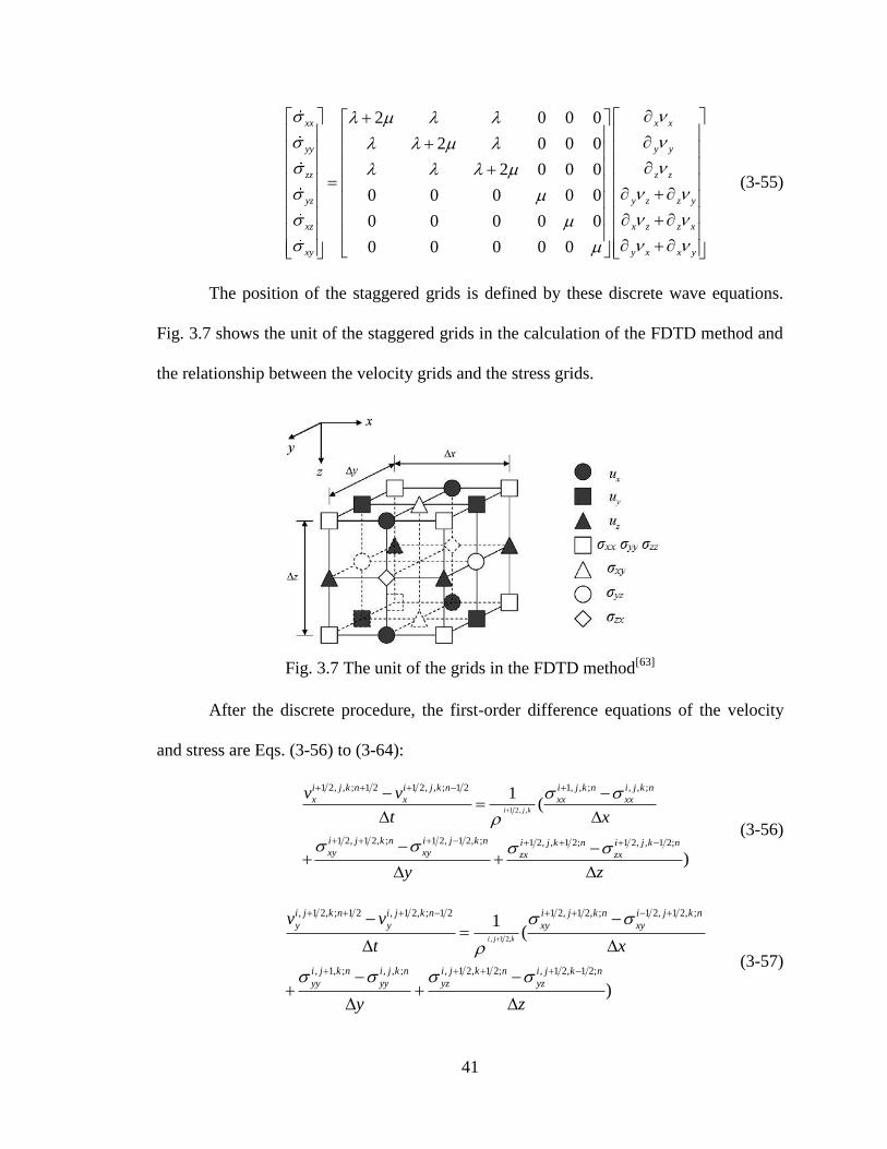
41
(3-55)
The position of the staggered grids is defined by these discrete wave equations.
Fig. 3.7 shows the unit of the staggered grids in the calculation of the FDTD method and
the relationship between the velocity grids and the stress grids.
After the discrete procedure, the first-order difference equations of the velocity
and stress are Eqs. (3-56) to (3-64):
(3-56)
(3-57)
2 0 0 0
2 0 0 0
2 0 0 0
0 0 0 0 0
0 0 0 0 0
0 0 0 0 0
xx x x
yy y y
zz z z
yz y z z y
xz x z z x
xy y x x y
1 2, ,
1 2, , ; 1 2 1 2, , ; 1 2 1, , ; , , ;
1 2, 1 2, ; 1 2, 1 2, ; 1 2, , 1 2; 1 2, , 1 2;
1(
)
i j k
i j k n i j k n i j k n i j k n
x x xx xx
i j k n i j k n i j k n i j k nxy xy zx zx
v v
t x
y z
, 1 2,
, 1 2, ; 1 2 , 1 2, ; 1 2 1 2, 1 2, ; 1 2, 1 2, ;
, 1, ; , , ; , 1 2, 1 2; , 1 2, 1 2;
1(
)
i j k
i j k n i j k n i j k n i j k n
y y xy xy
i j k n i j k n i j k n i j k n
yy yy yz yz
v v
t x
y z
Fig. 3.7 The unit of the grids in the FDTD method[63]
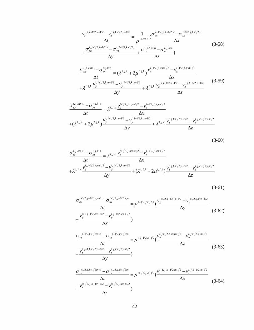
42
(3-58)
(3-59)
(3-60)
(3-61)
(3-62)
(3-63)
(3-64)
, , 1 2
1 2, , 1 2; 1 2, , 1 2;, , 1 2; 1 2 , , 1 2; 1 2
, 1 2, 1 2; , 1 2, 1 2; , , 1; , , ;
1(
)
i j k
i j k n i j k ni j k n i j k n
zx zxz z
i j k n i j k n i j k n i j k nyz yz zz zz
v v
t x
y z
, , ; 1 , , ; 1 2, , ; 1 2 1 2, , ; 1 2, , , ,
, 1 2, ; 1 2 , 1 2, ; 1 2 , , 1 2; 1 2 , , 1 2; 1 2, , , ,
( 2 )i j k n i j k n i j k n i j k n
i j k i j kxx xx x x
i j k n i j k n i j k n i j k ny yi j k i j k z z
v v
t x
v v v v
y z
, , ; 1 , , ; 1 2, , ; 1 2 1 2, , ; 1 2, ,
, 1 2, ; 1 2 , 1 2, ; 1 2 , , 1 2; 1 2 , , 1 2; 1 2, , , , , ,( 2 )
i j k n i j k n i j k n i j k nyy yy i j k x x
i j k n i j k n i j k n i j k ny yi j k i j k i j k z z
v v
t x
v v v v
y z
1 2, , ; 1 2 1 2, , ; 1 2, , ; 1 , , ;, ,
, 1 2, ; 1 2 , 1 2, ; 1 2 , , 1 2; 1 2 , , 1 2; 1 2, , , , , ,( 2 )
i j k n i j k ni j k n i j k ni j k x xzz zz
i j k n i j k n i j k n i j k ny yi j k i j k i j k z z
v v
t x
v v v v
y z
1 2, 1 2, ; 1 1 2, 1 2, ; 1 2, 1, ; 1 2 1 2, , ; 1 21 2, 1 2,
1, 1 2, ; 1 2 , 1 2, ; 1 2
(
)
i j k n i j k n i j k n i j k nxy xy i j k x x
i j k n i j k n
y y
v v
t y
v v
x
, 1 2, 1 2; 1 , 1 2, 1 2; , 1 2, 1; 1 2 , 1 2, ; 1 2
, 1 2, 1 2
, 1, 1 2; 1 2 , , 1 2; 1 2
(
)
i j k n i j k n i j k n i j k n
yz yz y yi j k
i j k n i j k n
z z
v v
t z
v v
y
1 2, , 1 2; 1 1 2, , 1 2; 1, , 1 2; 1 2 , , 1 2; 1 21 2, , 1 2
1 2, , 1; 1 2 1 2, , ; 1 2
(
)
i j k n i j k n i j k n i j k ni j kzx zx z z
i j k n i j k n
x x
v v
t x
v v
z
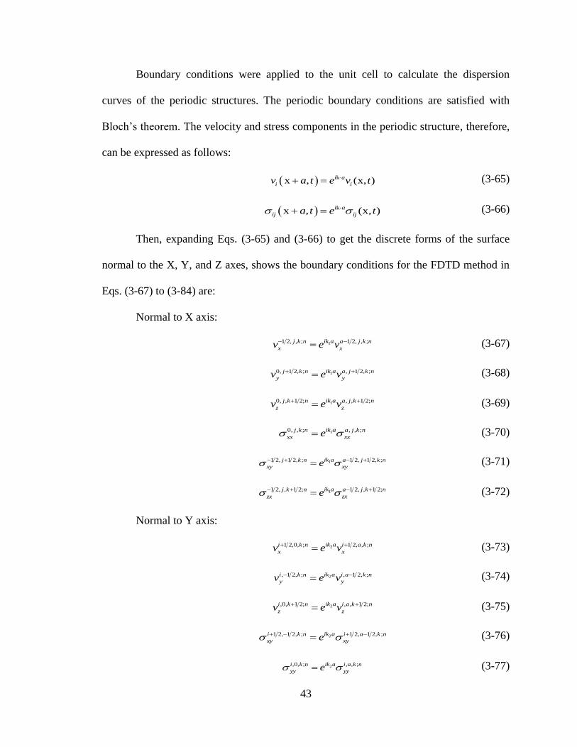
43
Boundary conditions were applied to the unit cell to calculate the dispersion
curves of the periodic structures. The periodic boundary conditions are satisfied with
Bloch’s theorem. The velocity and stress components in the periodic structure, therefore,
can be expressed as follows:
(3-65)
(3-66)
Then, expanding Eqs. (3-65) and (3-66) to get the discrete forms of the surface
normal to the X, Y, and Z axes, shows the boundary conditions for the FDTD method in
Eqs. (3-67) to (3-84) are:
Normal to X axis:
(3-67)
(3-68)
(3-69)
(3-70)
(3-71)
(3-72)
Normal to Y axis:
(3-73)
(3-74)
(3-75)
(3-76)
(3-77)
kx , (x, )i a
i iv a t e v t
kx , (x, )i a
ij ija t e t
11 2, , ; 1 2, , ;ik aj k n a j k n
x xv e v
10, 1 2, ; , 1 2, ;ik aj k n a j k n
y yv e v
10, , 1 2; , , 1 2;ik aj k n a j k n
z zv e v
10, , ; , , ;ik aj k n a j k n
xx xxe
11 2, 1 2, ; 1 2, 1 2, ;ik aj k n a j k n
xy xye
11 2, , 1 2; 1 2, , 1 2;ik aj k n a j k n
zx zxe
21 2,0, ; 1 2, , ;ik ai k n i a k n
x xv e v
2, 1 2, ; , 1 2, ;ik ai k n i a k n
y yv e v
2,0, 1 2; , , 1 2;ik ai k n i a k n
z zv e v
21 2, 1 2, ; 1 2, 1 2, ;ik ai k n i a k n
xy xye
2,0, ; , , ;ik ai k n i a k n
yy yye
44
(3-78)
Normal to Z axis:
(3-79)
(3-80)
(3-81)
(3-82)
(3-83)
(3-84)
Where k=(k1,k2,k3) are wave vectors.
Excitation from a single point of the computation region is considered as the
excitation. It is widely known that the spectrum of the delta-pulse is infinitely wide so
that it gives structural responses at any frequency. After the delta-pulse is introduced, the
excitation is turned off; however, owing to periodic boundary conditions, radiation exists
for infinite duration in the structure without absorption. In the case of delta-pulse, the
excitation function takes the following form:
(3-85)
After the pulse response of the structure is obtained, it should be analyzed. The
time-dependent response of the structure could be found at any point of the
computational domain. Next, the fast Fourier transform (FFT) is used to obtain the
discreet spectrum. Then, the resonant frequencies of the periodic structure can be
obtained. The resonant points are the existing peaks in the frequency spectra. When k
2, 1 2, 1 2; , 1 2, 1 2;ik ai k n i a k n
zy zye
31 2, ,0; 1 2, , ;ik ai j n i j a n
x xv e v
3, 1 2,0; , 1 2, ;ik ai j n i j a n
y yv e v
3, , 1 2; , , 1 2;ik ai j n i j a n
z zv e v
31 2, , 1 2; 1 2, , 1 2;ik ai j n i j a n
zx zxe
3, 1 2, 1 2; , 1 2, 1 2;ik ai j n i j k n
zy zye
3, ,0; , , ;ik ai j n i j a n
zz zze
0 0 0 0, , , 1x x y y z z t t
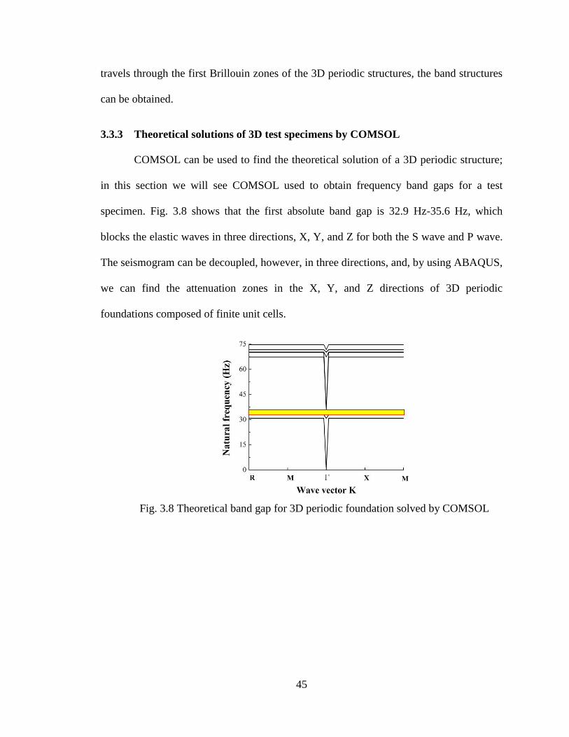
45
travels through the first Brillouin zones of the 3D periodic structures, the band structures
can be obtained.
3.3.3 Theoretical solutions of 3D test specimens by COMSOL
COMSOL can be used to find the theoretical solution of a 3D periodic structure;
in this section we will see COMSOL used to obtain frequency band gaps for a test
specimen. Fig. 3.8 shows that the first absolute band gap is 32.9 Hz-35.6 Hz, which
blocks the elastic waves in three directions, X, Y, and Z for both the S wave and P wave.
The seismogram can be decoupled, however, in three directions, and, by using ABAQUS,
we can find the attenuation zones in the X, Y, and Z directions of 3D periodic
foundations composed of finite unit cells.
Fig. 3.8 Theoretical band gap for 3D periodic foundation solved by COMSOL

47
4 FINITE ELEMENT MODELING OF PERIODIC FOUNDATIONS
This section shows parametric studies conducted for 1D, 2D, and 3D periodic
structures with infinite unit cells to obtain wider and lower band gaps for seismic
resistance. The factors for parametric study include material properties and geometric
properties such as density, Young’s modulus of materials, size of unit cells, etc. With the
results obtained from the parametric study, the test specimens of 1D, 2D, and 3D periodic
foundations with finite unit cells are designed according to the analysis results of the
parametric study. We see in this chapter the attenuation zones of 1D, 2D, and 3D periodic
foundations obtained using ABAQUS.
4.1 FE Modeling of 1D Layered Periodic Foundations
4.1.1 Parametric study of 1D periodic foundations
A periodic foundation is composed of two materials as one unit: the rubber layer
and the concrete layer. Many units repeat along the vertical direction to compose a 1D
periodic foundation; this kind of periodic foundation reduces dynamic response. The
effects of material and geometric properties of 1D periodic structures on the first band
gap are discussed in this section, with both longitudinal and transverse waves, using the
method mentioned in Section 3.1. Fig. 4.1 shows one unit cell of a 1D periodic structure
for parametric study: A is the rubber layer, and B is the concrete layer. The thickness
ratio is defined as the ratio between the thicknesses of layer A relative to that of layer B.
To conduct the parametric study, the parameter to be investigated is selected, and other
parameters are fixed. The relationship between the parameter to be investigated and the
first band gap can be plotted.

48
4.1.1.1 Material Properties
To study the material properties, the geometric properties are fixed as shown in
Table 4.1; the unit cell size is 0.4m, and the thickness ratio is 1. Fig. 4.2 to Fig. 4.5 shows
the effects of material properties on the frequency band gap with longitudinal wave input.
Table 4.1 The properties of 1D material parametric study
Parameters
Young’s
modulus of
rubber (Pa)
Young’s
modulus of
concrete
(Pa)
Density of
rubber
(kg/m3)
Density of
concrete
(kg/m3)
Unit cell
size (m)
Thickness
ratio
Young’s
modulus of
rubber (Pa)
Selected 3.14×10¹⁰
1300 2300 0.4 1
Young’s
modulus of
concrete
(Pa)
5.8×10⁵ Selected 1300 2300 0.4 1
Density of
rubber
(kg/m3)
5.8×10⁵ 3.14×10
10 Selected 2300 0.4 1
Density of
concrete
(kg/m3)
5.8×10⁵ 3.14×10
10 1300 Selected 0.4 1
Fig. 4.1 One unit cell of 1D periodic structure
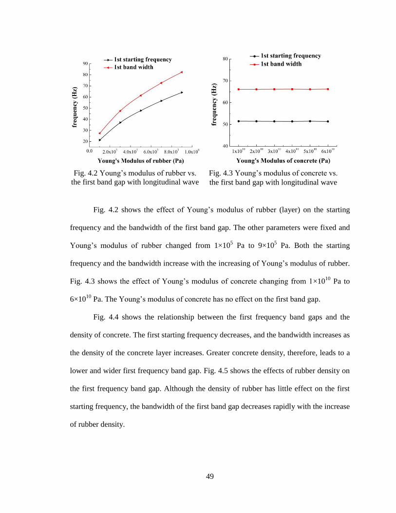
49
Fig. 4.2 shows the effect of Young’s modulus of rubber (layer) on the starting
frequency and the bandwidth of the first band gap. The other parameters were fixed and
Young’s modulus of rubber changed from 1×10⁵ Pa to 9×10
5 Pa. Both the starting
frequency and the bandwidth increase with the increasing of Young’s modulus of rubber.
Fig. 4.3 shows the effect of Young’s modulus of concrete changing from 1×10¹⁰
Pa to
6×10¹⁰
Pa. The Young’s modulus of concrete has no effect on the first band gap.
Fig. 4.4 shows the relationship between the first frequency band gaps and the
density of concrete. The first starting frequency decreases, and the bandwidth increases as
the density of the concrete layer increases. Greater concrete density, therefore, leads to a
lower and wider first frequency band gap. Fig. 4.5 shows the effects of rubber density on
the first frequency band gap. Although the density of rubber has little effect on the first
starting frequency, the bandwidth of the first band gap decreases rapidly with the increase
of rubber density.
Fig. 4.2 Young’s modulus of rubber vs.
the first band gap with longitudinal wave
Fig. 4.3 Young’s modulus of concrete vs.
the first band gap with longitudinal wave
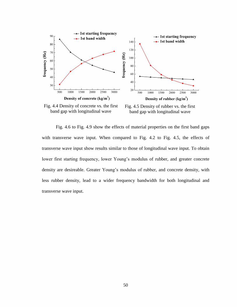
50
Fig. 4.6 to Fig. 4.9 show the effects of material properties on the first band gaps
with transverse wave input. When compared to Fig. 4.2 to Fig. 4.5, the effects of
transverse wave input show results similar to those of longitudinal wave input. To obtain
lower first starting frequency, lower Young’s modulus of rubber, and greater concrete
density are desireable. Greater Young’s modulus of rubber, and concrete density, with
less rubber density, lead to a wider frequency bandwidth for both longitudinal and
transverse wave input.
Fig. 4.4 Density of concrete vs. the first
band gap with longitudinal wave
Fig. 4.5 Density of rubber vs. the first
band gap with longitudinal wave
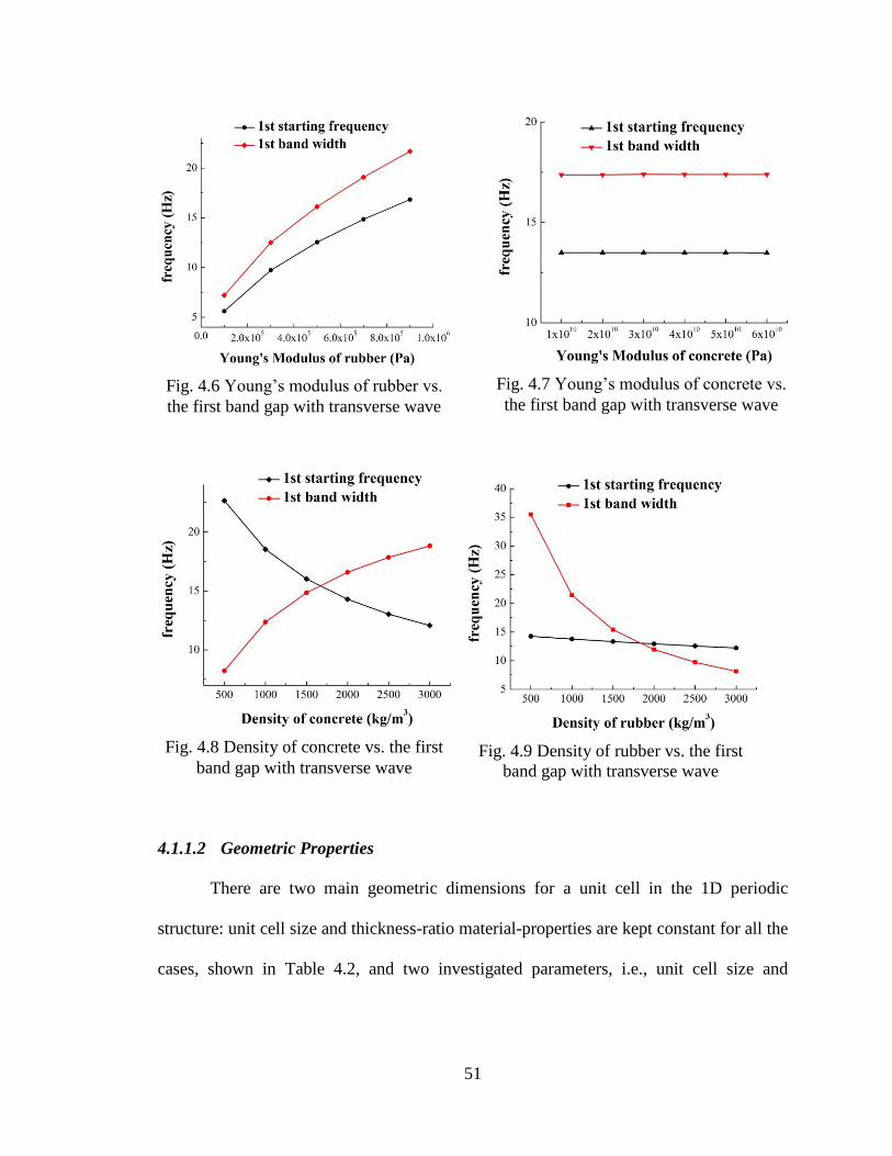
51
4.1.1.2 Geometric Properties
There are two main geometric dimensions for a unit cell in the 1D periodic
structure: unit cell size and thickness-ratio material-properties are kept constant for all the
cases, shown in Table 4.2, and two investigated parameters, i.e., unit cell size and
Fig. 4.6 Young’s modulus of rubber vs.
the first band gap with transverse wave
Fig. 4.7 Young’s modulus of concrete vs.
the first band gap with transverse wave
Fig. 4.8 Density of concrete vs. the first
band gap with transverse wave
Fig. 4.9 Density of rubber vs. the first
band gap with transverse wave
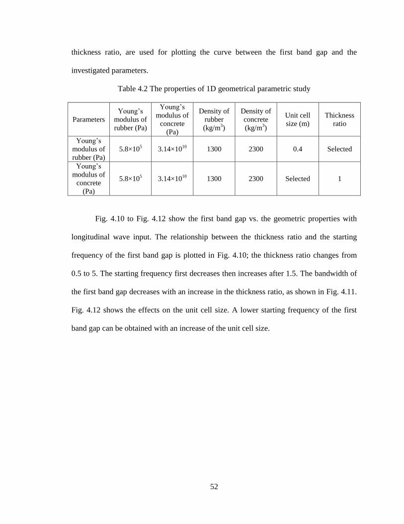
52
thickness ratio, are used for plotting the curve between the first band gap and the
investigated parameters.
Table 4.2 The properties of 1D geometrical parametric study
Parameters
Young’s
modulus of
rubber (Pa)
Young’s
modulus of
concrete
(Pa)
Density of
rubber
(kg/m3)
Density of
concrete
(kg/m3)
Unit cell
size (m)
Thickness
ratio
Young’s
modulus of
rubber (Pa)
5.8×10⁵ 3.14×10
10 1300 2300 0.4 Selected
Young’s
modulus of
concrete
(Pa)
5.8×10⁵ 3.14×10
10 1300 2300 Selected 1
Fig. 4.10 to Fig. 4.12 show the first band gap vs. the geometric properties with
longitudinal wave input. The relationship between the thickness ratio and the starting
frequency of the first band gap is plotted in Fig. 4.10; the thickness ratio changes from
0.5 to 5. The starting frequency first decreases then increases after 1.5. The bandwidth of
the first band gap decreases with an increase in the thickness ratio, as shown in Fig. 4.11.
Fig. 4.12 shows the effects on the unit cell size. A lower starting frequency of the first
band gap can be obtained with an increase of the unit cell size.
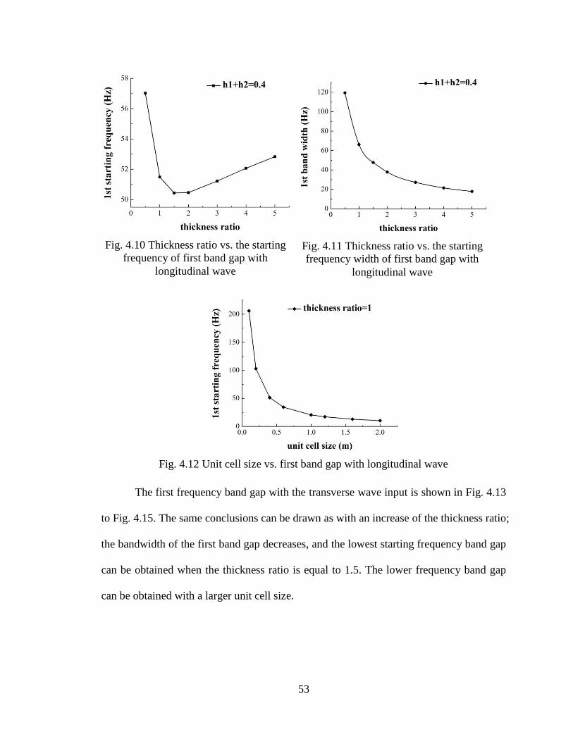
53
The first frequency band gap with the transverse wave input is shown in Fig. 4.13
to Fig. 4.15. The same conclusions can be drawn as with an increase of the thickness ratio;
the bandwidth of the first band gap decreases, and the lowest starting frequency band gap
can be obtained when the thickness ratio is equal to 1.5. The lower frequency band gap
can be obtained with a larger unit cell size.
Fig. 4.10 Thickness ratio vs. the starting
frequency of first band gap with
longitudinal wave
Fig. 4.11 Thickness ratio vs. the starting
frequency width of first band gap with
longitudinal wave
Fig. 4.12 Unit cell size vs. first band gap with longitudinal wave
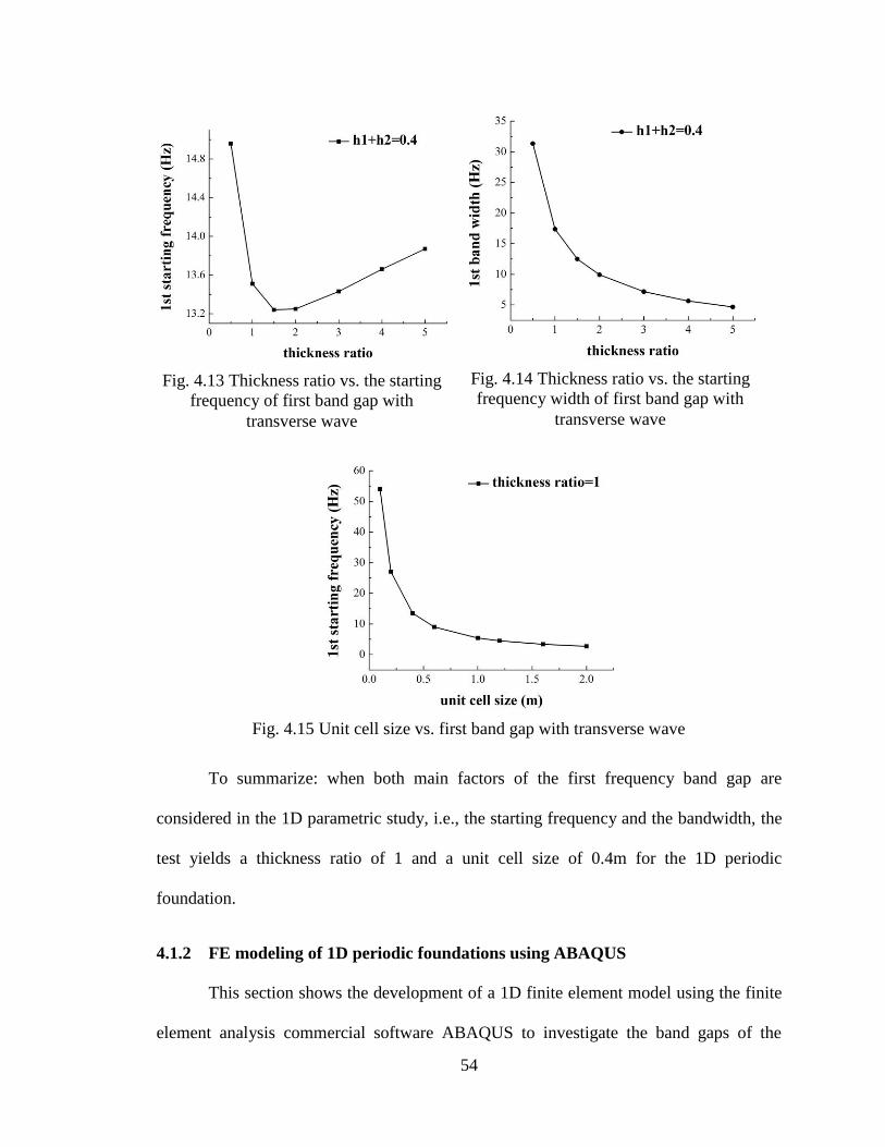
54
To summarize: when both main factors of the first frequency band gap are
considered in the 1D parametric study, i.e., the starting frequency and the bandwidth, the
test yields a thickness ratio of 1 and a unit cell size of 0.4m for the 1D periodic
foundation.
4.1.2 FE modeling of 1D periodic foundations using ABAQUS
This section shows the development of a 1D finite element model using the finite
element analysis commercial software ABAQUS to investigate the band gaps of the
Fig. 4.13 Thickness ratio vs. the starting
frequency of first band gap with
transverse wave
Fig. 4.14 Thickness ratio vs. the starting
frequency width of first band gap with
transverse wave
Fig. 4.15 Unit cell size vs. first band gap with transverse wave
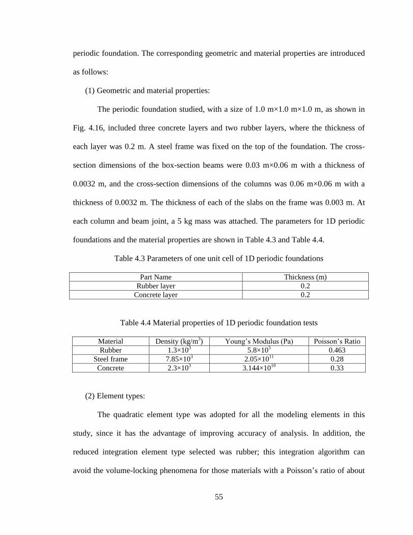
55
periodic foundation. The corresponding geometric and material properties are introduced
as follows:
(1) Geometric and material properties:
The periodic foundation studied, with a size of 1.0 m×1.0 m×1.0 m, as shown in
Fig. 4.16, included three concrete layers and two rubber layers, where the thickness of
each layer was 0.2 m. A steel frame was fixed on the top of the foundation. The cross-
section dimensions of the box-section beams were 0.03 m×0.06 m with a thickness of
0.0032 m, and the cross-section dimensions of the columns was 0.06 m×0.06 m with a
thickness of 0.0032 m. The thickness of each of the slabs on the frame was 0.003 m. At
each column and beam joint, a 5 kg mass was attached. The parameters for 1D periodic
foundations and the material properties are shown in Table 4.3 and Table 4.4.
Table 4.3 Parameters of one unit cell of 1D periodic foundations
Part Name Thickness (m)
Rubber layer 0.2
Concrete layer 0.2
Table 4.4 Material properties of 1D periodic foundation tests
Material Density (kg/m3) Young’s Modulus (Pa) Poisson’s Ratio
Rubber 1.3×10³ 5.8×10
5 0.463
Steel frame 7.85×10³ 2.05×10
11 0.28
Concrete 2.3×10³ 3.144×10
10 0.33
(2) Element types:
The quadratic element type was adopted for all the modeling elements in this
study, since it has the advantage of improving accuracy of analysis. In addition, the
reduced integration element type selected was rubber; this integration algorithm can
avoid the volume-locking phenomena for those materials with a Poisson’s ratio of about
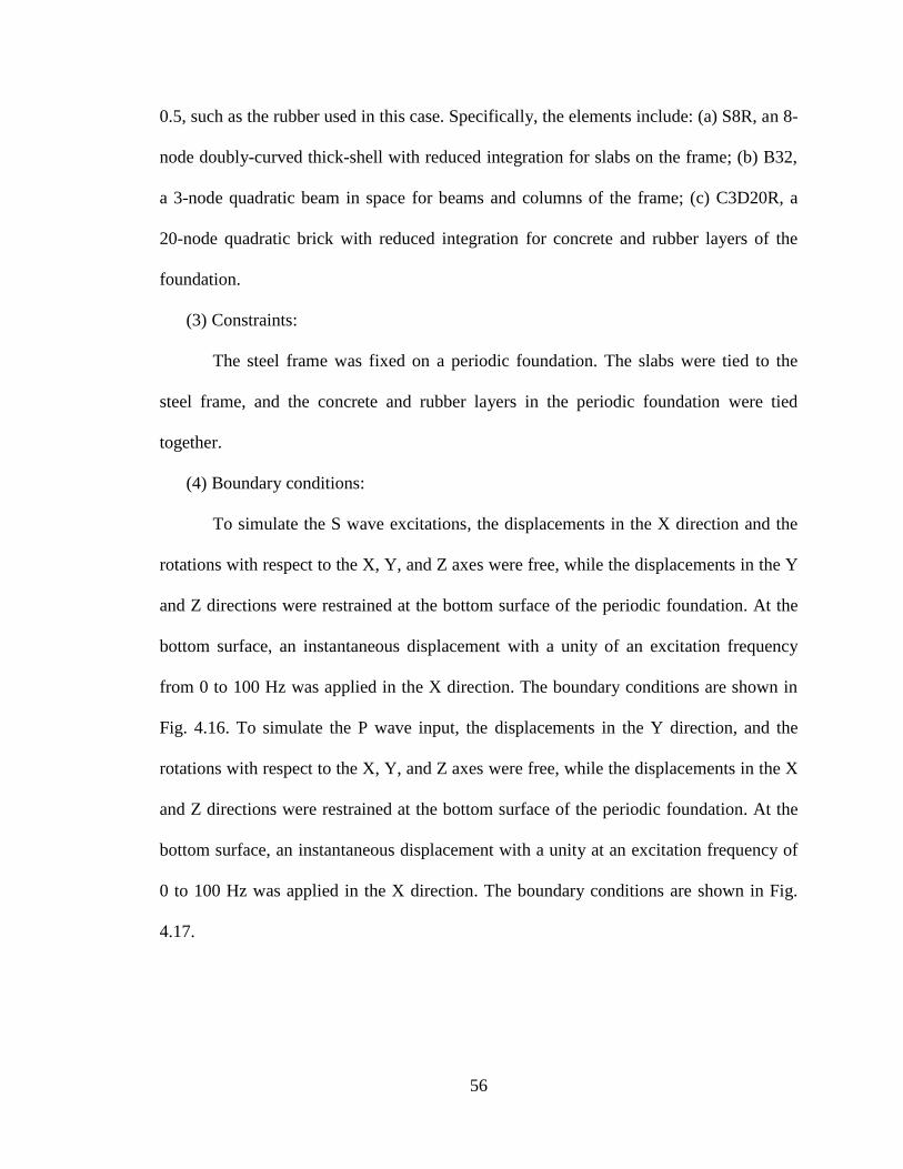
56
0.5, such as the rubber used in this case. Specifically, the elements include: (a) S8R, an 8-
node doubly-curved thick-shell with reduced integration for slabs on the frame; (b) B32,
a 3-node quadratic beam in space for beams and columns of the frame; (c) C3D20R, a
20-node quadratic brick with reduced integration for concrete and rubber layers of the
foundation.
(3) Constraints:
The steel frame was fixed on a periodic foundation. The slabs were tied to the
steel frame, and the concrete and rubber layers in the periodic foundation were tied
together.
(4) Boundary conditions:
To simulate the S wave excitations, the displacements in the X direction and the
rotations with respect to the X, Y, and Z axes were free, while the displacements in the Y
and Z directions were restrained at the bottom surface of the periodic foundation. At the
bottom surface, an instantaneous displacement with a unity of an excitation frequency
from 0 to 100 Hz was applied in the X direction. The boundary conditions are shown in
Fig. 4.16. To simulate the P wave input, the displacements in the Y direction, and the
rotations with respect to the X, Y, and Z axes were free, while the displacements in the X
and Z directions were restrained at the bottom surface of the periodic foundation. At the
bottom surface, an instantaneous displacement with a unity at an excitation frequency of
0 to 100 Hz was applied in the X direction. The boundary conditions are shown in Fig.
4.17.
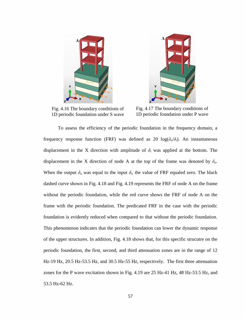
57
To assess the efficiency of the periodic foundation in the frequency domain, a
frequency response function (FRF) was defined as 20 log(δo/δi). An instantaneous
displacement in the X direction with amplitude of δi was applied at the bottom. The
displacement in the X direction of node A at the top of the frame was denoted by δo.
When the output δo was equal to the input δi, the value of FRF equaled zero. The black
dashed curve shown in Fig. 4.18 and Fig. 4.19 represents the FRF of node A on the frame
without the periodic foundation, while the red curve shows the FRF of node A on the
frame with the periodic foundation. The predicated FRF in the case with the periodic
foundation is evidently reduced when compared to that without the periodic foundation.
This phenomenon indicates that the periodic foundation can lower the dynamic response
of the upper structures. In addition, Fig. 4.18 shows that, for this specific strucutre on the
periodic foundation, the first, second, and third attenuation zones are in the range of 12
Hz-19 Hz, 20.5 Hz-53.5 Hz, and 30.5 Hz-55 Hz, respectively. The first three attenuation
zones for the P wave excitation shown in Fig. 4.19 are 25 Hz-41 Hz, 48 Hz-53.5 Hz, and
53.5 Hz-62 Hz.
Fig. 4.16 The boundary conditions of
1D periodic foundation under S wave
Fig. 4.17 The boundary conditions of
1D periodic foundation under P wave
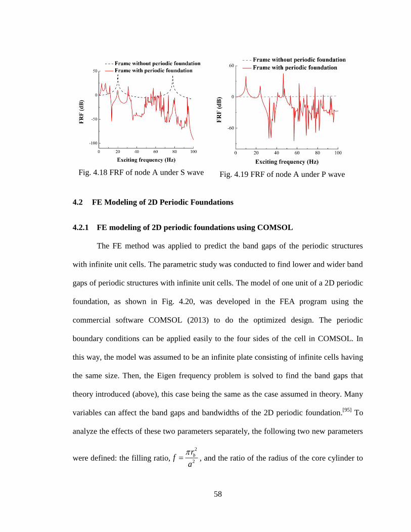
58
4.2 FE Modeling of 2D Periodic Foundations
4.2.1 FE modeling of 2D periodic foundations using COMSOL
The FE method was applied to predict the band gaps of the periodic structures
with infinite unit cells. The parametric study was conducted to find lower and wider band
gaps of periodic structures with infinite unit cells. The model of one unit of a 2D periodic
foundation, as shown in Fig. 4.20, was developed in the FEA program using the
commercial software COMSOL (2013) to do the optimized design. The periodic
boundary conditions can be applied easily to the four sides of the cell in COMSOL. In
this way, the model was assumed to be an infinite plate consisting of infinite cells having
the same size. Then, the Eigen frequency problem is solved to find the band gaps that
theory introduced (above), this case being the same as the case assumed in theory. Many
variables can affect the band gaps and bandwidths of the 2D periodic foundation.[95]
To
analyze the effects of these two parameters separately, the following two new parameters
were defined: the filling ratio, , and the ratio of the radius of the core cylinder to
2
2
brfa
Fig. 4.18 FRF of node A under S wave
Fig. 4.19 FRF of node A under P wave
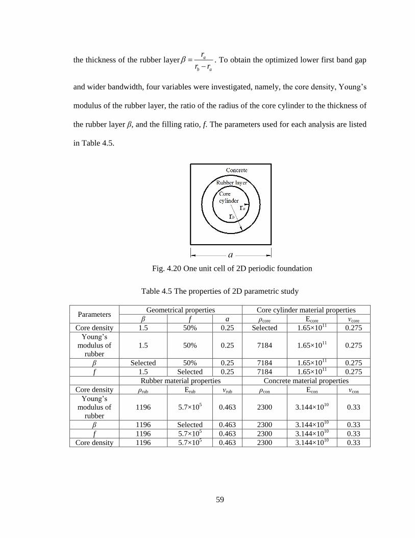
59
the thickness of the rubber layer . To obtain the optimized lower first band gap
and wider bandwidth, four variables were investigated, namely, the core density, Young’s
modulus of the rubber layer, the ratio of the radius of the core cylinder to the thickness of
the rubber layer β, and the filling ratio, f. The parameters used for each analysis are listed
in Table 4.5.
Table 4.5 The properties of 2D parametric study
Parameters Geometrical properties Core cylinder material properties
β f a ρcore Ecore νcore
Core density 1.5 50% 0.25 Selected 1.65×10¹¹
0.275
Young’s
modulus of
rubber
1.5 50% 0.25 7184 1.65×10¹¹
0.275
β Selected 50% 0.25 7184 1.65×10¹¹
0.275
f 1.5 Selected 0.25 7184 1.65×10¹¹
0.275
Rubber material properties Concrete material properties
Core density ρrub Erub νrub ρcon Econ νcon
Young’s
modulus of
rubber
1196 5.7×10⁵ 0.463 2300 3.144×10
10 0.33
β 1196 Selected 0.463 2300 3.144×10¹⁰
0.33
f 1196 5.7×10⁵ 0.463 2300 3.144×10
10 0.33
Core density 1196 5.7×10⁵ 0.463 2300 3.144×10
10 0.33
a
b a
r
r r
Fig. 4.20 One unit cell of 2D periodic foundation
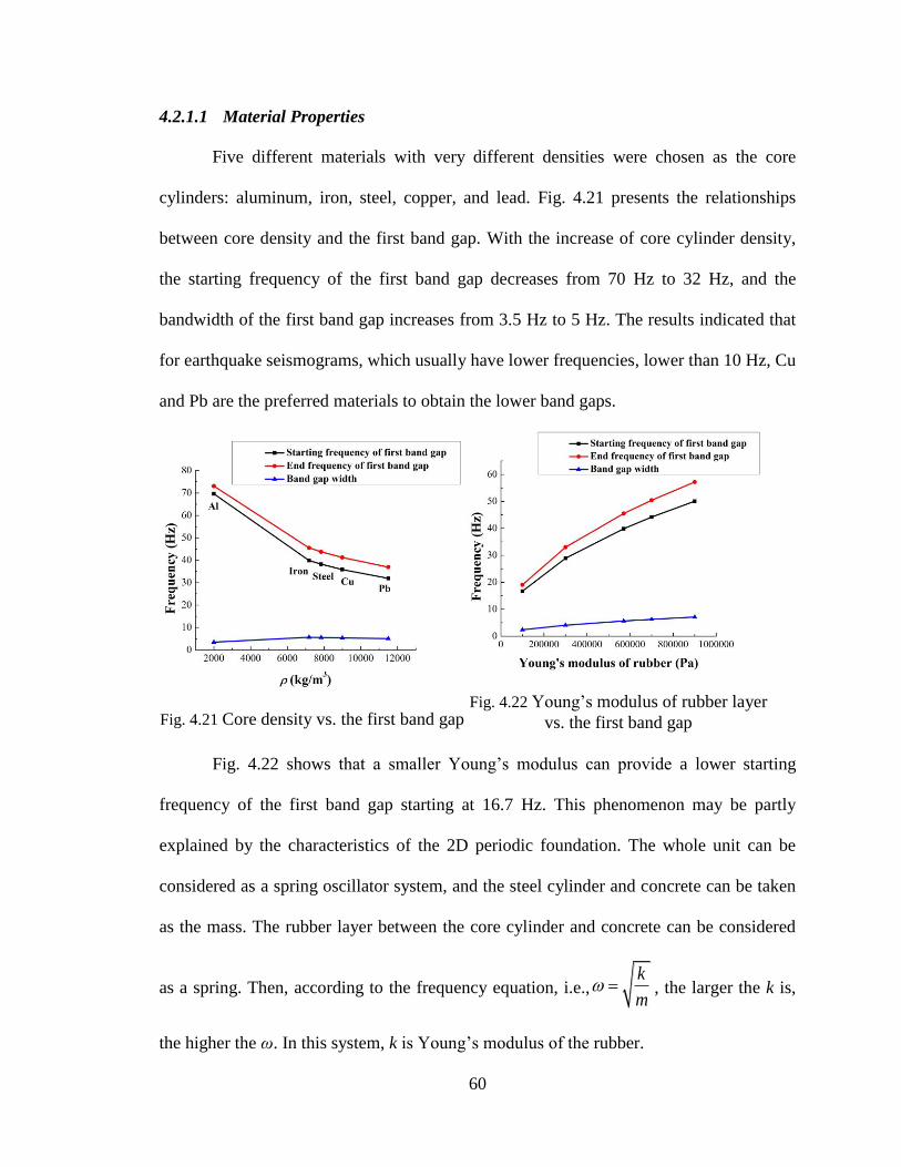
60
4.2.1.1 Material Properties
Five different materials with very different densities were chosen as the core
cylinders: aluminum, iron, steel, copper, and lead. Fig. 4.21 presents the relationships
between core density and the first band gap. With the increase of core cylinder density,
the starting frequency of the first band gap decreases from 70 Hz to 32 Hz, and the
bandwidth of the first band gap increases from 3.5 Hz to 5 Hz. The results indicated that
for earthquake seismograms, which usually have lower frequencies, lower than 10 Hz, Cu
and Pb are the preferred materials to obtain the lower band gaps.
Fig. 4.22 shows that a smaller Young’s modulus can provide a lower starting
frequency of the first band gap starting at 16.7 Hz. This phenomenon may be partly
explained by the characteristics of the 2D periodic foundation. The whole unit can be
considered as a spring oscillator system, and the steel cylinder and concrete can be taken
as the mass. The rubber layer between the core cylinder and concrete can be considered
as a spring. Then, according to the frequency equation, i.e., , the larger the k is,
the higher the ω. In this system, k is Young’s modulus of the rubber.
k
m
Fig. 4.21 Core density vs. the first band gap
Fig. 4.22 Young’s modulus of rubber layer
vs. the first band gap
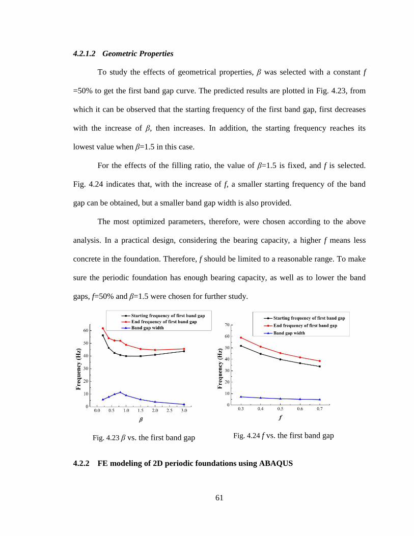
61
4.2.1.2 Geometric Properties
To study the effects of geometrical properties, β was selected with a constant f
=50% to get the first band gap curve. The predicted results are plotted in Fig. 4.23, from
which it can be observed that the starting frequency of the first band gap, first decreases
with the increase of β, then increases. In addition, the starting frequency reaches its
lowest value when β=1.5 in this case.
For the effects of the filling ratio, the value of β=1.5 is fixed, and f is selected.
Fig. 4.24 indicates that, with the increase of f, a smaller starting frequency of the band
gap can be obtained, but a smaller band gap width is also provided.
The most optimized parameters, therefore, were chosen according to the above
analysis. In a practical design, considering the bearing capacity, a higher f means less
concrete in the foundation. Therefore, f should be limited to a reasonable range. To make
sure the periodic foundation has enough bearing capacity, as well as to lower the band
gaps, f=50% and β=1.5 were chosen for further study.
4.2.2 FE modeling of 2D periodic foundations using ABAQUS
Fig. 4.23 β vs. the first band gap
Fig. 4.24 f vs. the first band gap
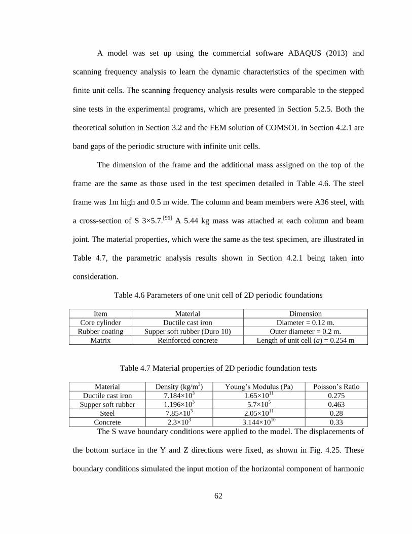
62
A model was set up using the commercial software ABAQUS (2013) and
scanning frequency analysis to learn the dynamic characteristics of the specimen with
finite unit cells. The scanning frequency analysis results were comparable to the stepped
sine tests in the experimental programs, which are presented in Section 5.2.5. Both the
theoretical solution in Section 3.2 and the FEM solution of COMSOL in Section 4.2.1 are
band gaps of the periodic structure with infinite unit cells.
The dimension of the frame and the additional mass assigned on the top of the
frame are the same as those used in the test specimen detailed in Table 4.6. The steel
frame was 1m high and 0.5 m wide. The column and beam members were A36 steel, with
a cross-section of S 3×5.7.[96]
A 5.44 kg mass was attached at each column and beam
joint. The material properties, which were the same as the test specimen, are illustrated in
Table 4.7, the parametric analysis results shown in Section 4.2.1 being taken into
consideration.
Table 4.6 Parameters of one unit cell of 2D periodic foundations
Item Material Dimension
Core cylinder Ductile cast iron Diameter = 0.12 m.
Rubber coating Supper soft rubber (Duro 10) Outer diameter = 0.2 m.
Matrix Reinforced concrete Length of unit cell (a) = 0.254 m
Table 4.7 Material properties of 2D periodic foundation tests
Material Density (kg/m3) Young’s Modulus (Pa) Poisson’s Ratio
Ductile cast iron 7.184×10³ 1.65×10
11 0.275
Supper soft rubber 1.196×10³ 5.7×10
5 0.463
Steel 7.85×10³ 2.05×10
11 0.28
Concrete 2.3×10³ 3.144×10
10 0.33
The S wave boundary conditions were applied to the model. The displacements of
the bottom surface in the Y and Z directions were fixed, as shown in Fig. 4.25. These
boundary conditions simulated the input motion of the horizontal component of harmonic
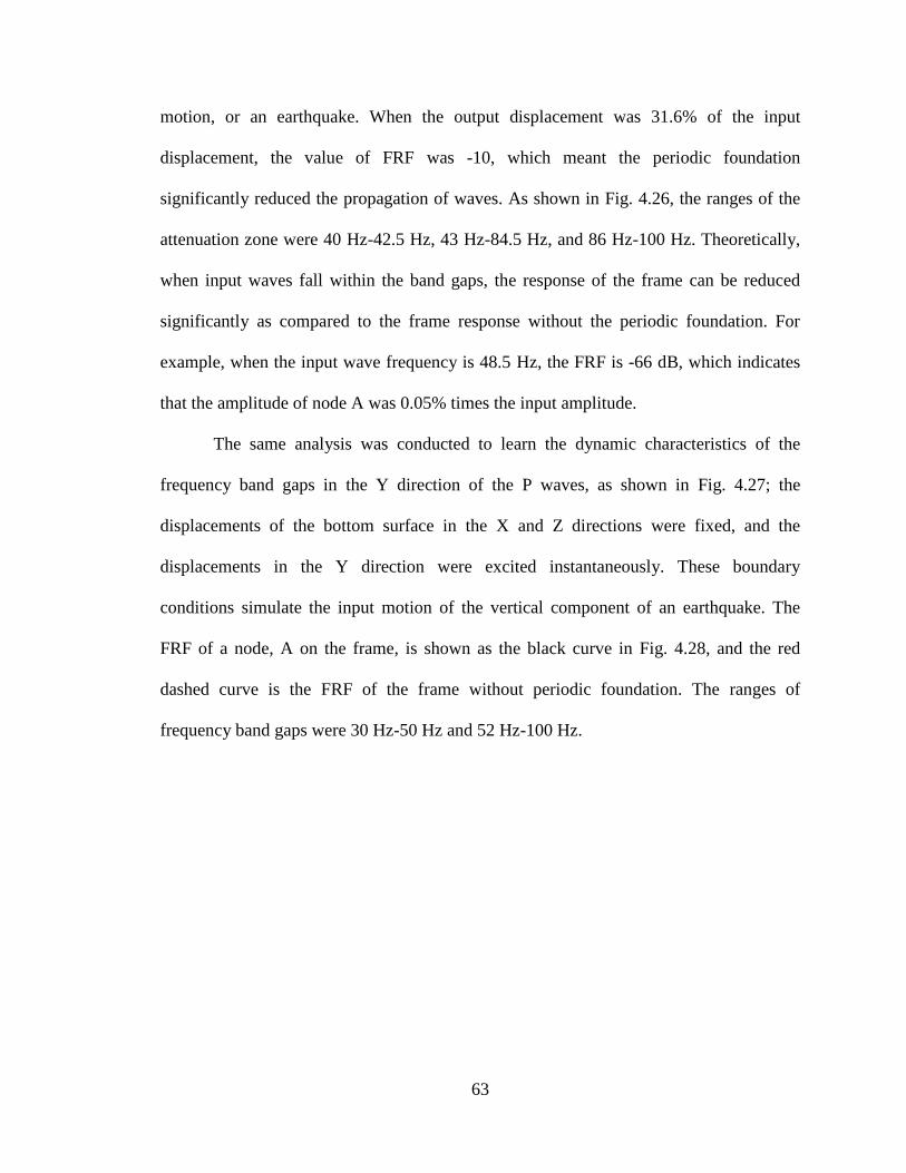
63
motion, or an earthquake. When the output displacement was 31.6% of the input
displacement, the value of FRF was -10, which meant the periodic foundation
significantly reduced the propagation of waves. As shown in Fig. 4.26, the ranges of the
attenuation zone were 40 Hz-42.5 Hz, 43 Hz-84.5 Hz, and 86 Hz-100 Hz. Theoretically,
when input waves fall within the band gaps, the response of the frame can be reduced
significantly as compared to the frame response without the periodic foundation. For
example, when the input wave frequency is 48.5 Hz, the FRF is -66 dB, which indicates
that the amplitude of node A was 0.05% times the input amplitude.
The same analysis was conducted to learn the dynamic characteristics of the
frequency band gaps in the Y direction of the P waves, as shown in Fig. 4.27; the
displacements of the bottom surface in the X and Z directions were fixed, and the
displacements in the Y direction were excited instantaneously. These boundary
conditions simulate the input motion of the vertical component of an earthquake. The
FRF of a node, A on the frame, is shown as the black curve in Fig. 4.28, and the red
dashed curve is the FRF of the frame without periodic foundation. The ranges of
frequency band gaps were 30 Hz-50 Hz and 52 Hz-100 Hz.
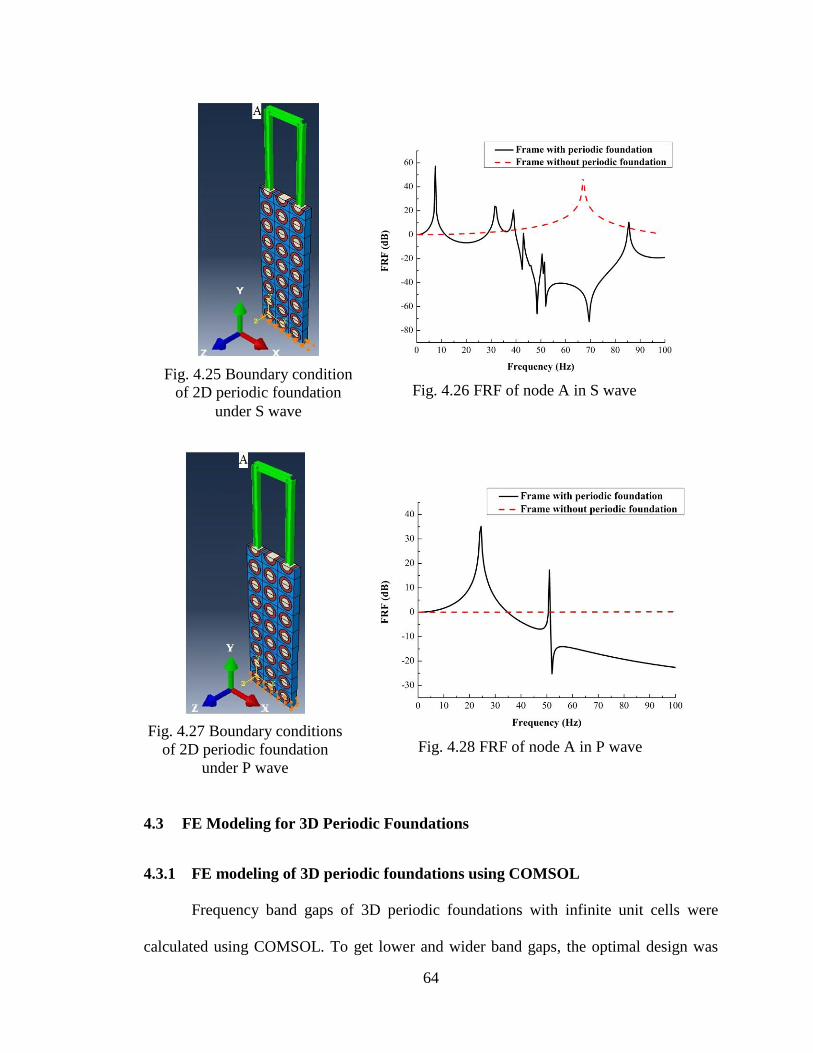
64
4.3 FE Modeling for 3D Periodic Foundations
4.3.1 FE modeling of 3D periodic foundations using COMSOL
Frequency band gaps of 3D periodic foundations with infinite unit cells were
calculated using COMSOL. To get lower and wider band gaps, the optimal design was
Fig. 4.25 Boundary condition
of 2D periodic foundation
under S wave
Fig. 4.26 FRF of node A in S wave
Fig. 4.27 Boundary conditions
of 2D periodic foundation
under P wave
Fig. 4.28 FRF of node A in P wave
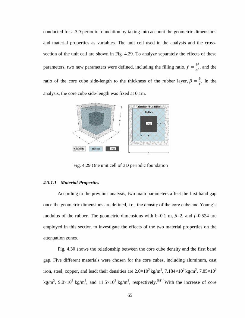
65
conducted for a 3D periodic foundation by taking into account the geometric dimensions
and material properties as variables. The unit cell used in the analysis and the cross-
section of the unit cell are shown in Fig. 4.29. To analyze separately the effects of these
parameters, two new parameters were defined, including the filling ratio,
, and the
ratio of the core cube side-length to the thickness of the rubber layer,
. In the
analysis, the core cube side-length was fixed at 0.1m.
4.3.1.1 Material Properties
According to the previous analysis, two main parameters affect the first band gap
once the geometric dimensions are defined, i.e., the density of the core cube and Young’s
modulus of the rubber. The geometric dimensions with b=0.1 m, β=2, and f=0.524 are
employed in this section to investigate the effects of the two material properties on the
attenuation zones.
Fig. 4.30 shows the relationship between the core cube density and the first band
gap. Five different materials were chosen for the core cubes, including aluminum, cast
iron, steel, copper, and lead; their densities are 2.0×10³
kg/m3, 7.184×10
3 kg/m
3, 7.85×10
3
kg/m3, 9.0×10
3 kg/m
3, and 11.5×10
3 kg/m
3, respectively.
[81] With the increase of core
Fig. 4.29 One unit cell of 3D periodic foundation
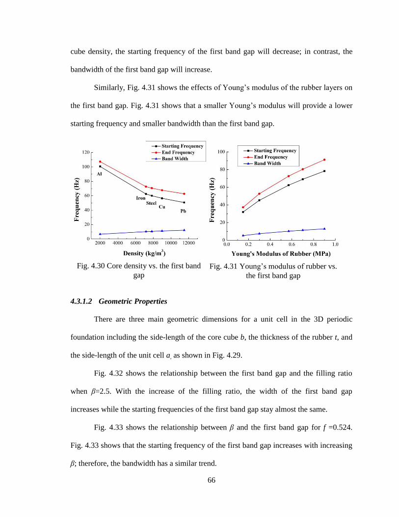
66
cube density, the starting frequency of the first band gap will decrease; in contrast, the
bandwidth of the first band gap will increase.
Similarly, Fig. 4.31 shows the effects of Young’s modulus of the rubber layers on
the first band gap. Fig. 4.31 shows that a smaller Young’s modulus will provide a lower
starting frequency and smaller bandwidth than the first band gap.
4.3.1.2 Geometric Properties
There are three main geometric dimensions for a unit cell in the 3D periodic
foundation including the side-length of the core cube b, the thickness of the rubber t, and
the side-length of the unit cell a, as shown in Fig. 4.29.
Fig. 4.32 shows the relationship between the first band gap and the filling ratio
when β=2.5. With the increase of the filling ratio, the width of the first band gap
increases while the starting frequencies of the first band gap stay almost the same.
Fig. 4.33 shows the relationship between β and the first band gap for f =0.524.
Fig. 4.33 shows that the starting frequency of the first band gap increases with increasing
β; therefore, the bandwidth has a similar trend.
Fig. 4.30 Core density vs. the first band
gap
Fig. 4.31 Young’s modulus of rubber vs.
the first band gap
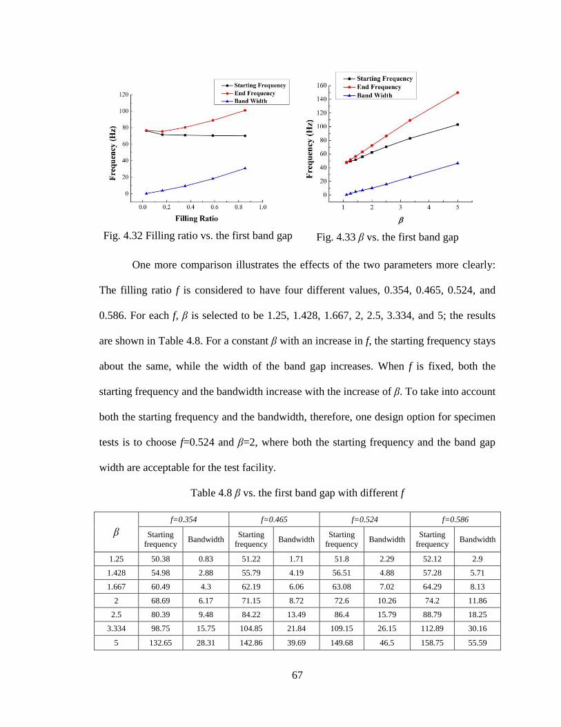
67
One more comparison illustrates the effects of the two parameters more clearly:
The filling ratio f is considered to have four different values, 0.354, 0.465, 0.524, and
0.586. For each f, β is selected to be 1.25, 1.428, 1.667, 2, 2.5, 3.334, and 5; the results
are shown in Table 4.8. For a constant β with an increase in f, the starting frequency stays
about the same, while the width of the band gap increases. When f is fixed, both the
starting frequency and the bandwidth increase with the increase of β. To take into account
both the starting frequency and the bandwidth, therefore, one design option for specimen
tests is to choose f=0.524 and β=2, where both the starting frequency and the band gap
width are acceptable for the test facility.
Table 4.8 β vs. the first band gap with different f
β
f=0.354 f=0.465 f=0.524 f=0.586
Starting
frequency Bandwidth
Starting
frequency Bandwidth
Starting
frequency Bandwidth
Starting
frequency Bandwidth
1.25 50.38 0.83 51.22 1.71 51.8 2.29 52.12 2.9
1.428 54.98 2.88 55.79 4.19 56.51 4.88 57.28 5.71
1.667 60.49 4.3 62.19 6.06 63.08 7.02 64.29 8.13
2 68.69 6.17 71.15 8.72 72.6 10.26 74.2 11.86
2.5 80.39 9.48 84.22 13.49 86.4 15.79 88.79 18.25
3.334 98.75 15.75 104.85 21.84 109.15 26.15 112.89 30.16
5 132.65 28.31 142.86 39.69 149.68 46.5 158.75 55.59
Fig. 4.32 Filling ratio vs. the first band gap
Fig. 4.33 β vs. the first band gap
68
4.3.2 FE modeling of 3D periodic foundations using ABAQUS
The ABAQUS models were developed to determine the dynamic characteristics
of the specimens. Fig. 4.29 shows one unit cell of the periodic foundation and the cross-
section. The dimensions of the steel column and the additional mass assigned on the top
of the column were the same as those used in the test specimen, as detailed in Table 4.9.
The steel column was 1m high; the column member was A36 steel, with a cross-section
of S 3×5.7,[96]
and the beam was 0.6m with the same cross-section as the column. A
5.44kg mass was added to the beam and column-joint or the top of the column to reduce
the natural frequency of the superstructure. The material properties, which were the same
as the test specimen, are also illustrated in Table 4.10.
Table 4.9 Parameters of one unit cell of 3D periodic foundations
Part name Material Length of side
core cube ductile cast iron b=102 mm
polyurethane coating polyurethane (Oo 30) b +2t=203 mm
matrix concrete a=305 mm
Table 4.10 Material properties of 3D periodic foundation tests
Material Density (kg/m3) Young’s Modulus (Pa) Poisson’s Ratio
Ductile cast iron 7.184×10³ 1.65×10
11 0.275
Polyurethane 1.277×10³ 1.586×10
5 0.463
Steel column 7.85×10³ 2.05×10
11 0.28
Concrete 2.3×10³ 4.0×10
10 0.33
The dynamic characteristics under an S wave were studied first. Fig. 4.34 presents
the 3D periodic foundation with a frame on it; the 3D periodic foundation was composed
of 5 by 5 unit cells, shown as Case 1. The 3D periodic foundation composed of 3 by 3
unit cells are shown as Case 2. To simplify the model, a periodic foundation with a
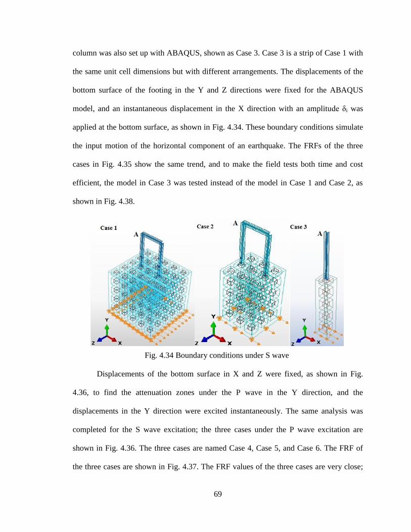
69
column was also set up with ABAQUS, shown as Case 3. Case 3 is a strip of Case 1 with
the same unit cell dimensions but with different arrangements. The displacements of the
bottom surface of the footing in the Y and Z directions were fixed for the ABAQUS
model, and an instantaneous displacement in the X direction with an amplitude δi was
applied at the bottom surface, as shown in Fig. 4.34. These boundary conditions simulate
the input motion of the horizontal component of an earthquake. The FRFs of the three
cases in Fig. 4.35 show the same trend, and to make the field tests both time and cost
efficient, the model in Case 3 was tested instead of the model in Case 1 and Case 2, as
shown in Fig. 4.38.
Displacements of the bottom surface in X and Z were fixed, as shown in Fig.
4.36, to find the attenuation zones under the P wave in the Y direction, and the
displacements in the Y direction were excited instantaneously. The same analysis was
completed for the S wave excitation; the three cases under the P wave excitation are
shown in Fig. 4.36. The three cases are named Case 4, Case 5, and Case 6. The FRF of
the three cases are shown in Fig. 4.37. The FRF values of the three cases are very close;
Fig. 4.34 Boundary conditions under S wave

70
therefore, Case 3 and Case 6 can predict the attenuation zones of the six cases.
Considering cost and time efficiency, the 3D periodic foundation can be simplified as
shown in Fig. 4.38.
Fig. 4.35 FRF under S wave
Fig. 4.36 Boundary conditions under P wave
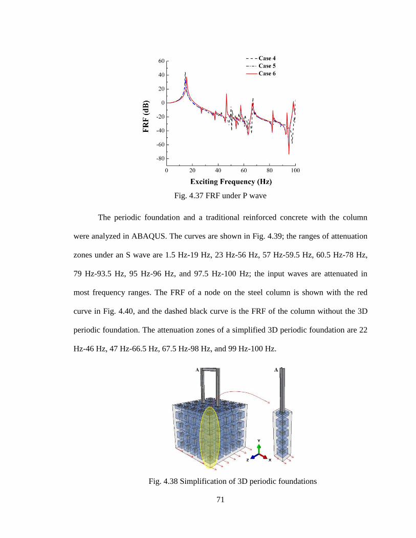
71
The periodic foundation and a traditional reinforced concrete with the column
were analyzed in ABAQUS. The curves are shown in Fig. 4.39; the ranges of attenuation
zones under an S wave are 1.5 Hz-19 Hz, 23 Hz-56 Hz, 57 Hz-59.5 Hz, 60.5 Hz-78 Hz,
79 Hz-93.5 Hz, 95 Hz-96 Hz, and 97.5 Hz-100 Hz; the input waves are attenuated in
most frequency ranges. The FRF of a node on the steel column is shown with the red
curve in Fig. 4.40, and the dashed black curve is the FRF of the column without the 3D
periodic foundation. The attenuation zones of a simplified 3D periodic foundation are 22
Hz-46 Hz, 47 Hz-66.5 Hz, 67.5 Hz-98 Hz, and 99 Hz-100 Hz.
Fig. 4.37 FRF under P wave
Fig. 4.38 Simplification of 3D periodic foundations
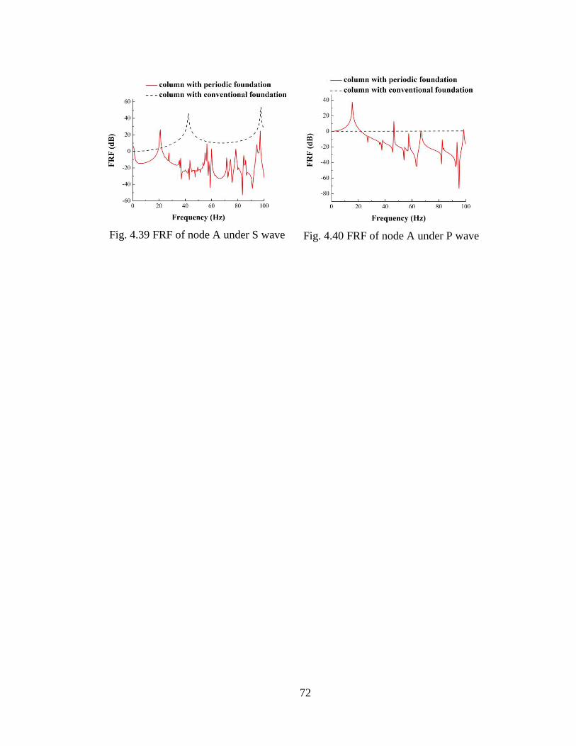
72
Fig. 4.39 FRF of node A under S wave
Fig. 4.40 FRF of node A under P wave
73
5 EXPERIMENTAL PROGRAM
In this chapter, the experimental program of 1D, 2D, and 3D periodic foundations
are introduced in Section 5.1, Section 5.2, and Section 5.3, respectively. The material
properties, test setup, and test procedures are illustrated.
5.1 Experimental Program of 1D Layered Periodic Foundations
5.1.1 1D layered periodic foundations specimen and test setup
The experimental program of 1D layered periodic foundation was performed in
the National Center for Research on Earthquake Engineering (NCREE) in Taiwan. To
test the 1D periodic foundation, two specimens were prepared. Specimen A was a three
story steel frame. The steel frame was fixed on the shake table. A mass of 20kg was
added for each floor. The cross-section of the columns in the steel frames was a square
tube with a sectional dimension of 6 cm (breadth) × 6 cm (depth) × 0.32 cm (thickness);
the cross-section of the beams was a rectangular tube with a sectional dimension of 3 cm
(breadth) × 6 cm (depth) × 0.32 cm (thickness), and the thickness of the slabs was 0.3 cm.
The height and plane dimensions of each story of the steel frames were 30 cm and 60 cm
by 60 cm, respectively. Specimen B was a steel frame of the same design as that of
Specimen A, but it was fixed on a 1D layered periodic bearing. The 1D periodic
foundation was composed of three concrete layers and two rubber layers with the
material properties as listed in Table 5.1. The thickness of each layer was 0.2 m, and the
dimension of each layer was 1 m×1 m. Fig. 5.1 shows the test specimens and the shake
table. The concrete layers and rubber layers were bonded together by polyurethane (PU)
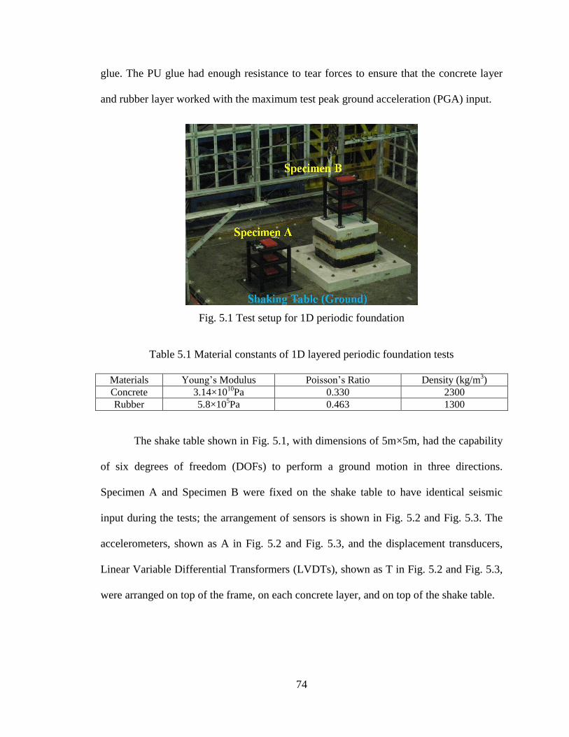
74
glue. The PU glue had enough resistance to tear forces to ensure that the concrete layer
and rubber layer worked with the maximum test peak ground acceleration (PGA) input.
Table 5.1 Material constants of 1D layered periodic foundation tests
Materials Young’s Modulus Poisson’s Ratio Density (kg/m3)
Concrete 3.14×10¹⁰
Pa 0.330 2300
Rubber 5.8×10⁵Pa 0.463 1300
The shake table shown in Fig. 5.1, with dimensions of 5m×5m, had the capability
of six degrees of freedom (DOFs) to perform a ground motion in three directions.
Specimen A and Specimen B were fixed on the shake table to have identical seismic
input during the tests; the arrangement of sensors is shown in Fig. 5.2 and Fig. 5.3. The
accelerometers, shown as A in Fig. 5.2 and Fig. 5.3, and the displacement transducers,
Linear Variable Differential Transformers (LVDTs), shown as T in Fig. 5.2 and Fig. 5.3,
were arranged on top of the frame, on each concrete layer, and on top of the shake table.
Fig. 5.1 Test setup for 1D periodic foundation
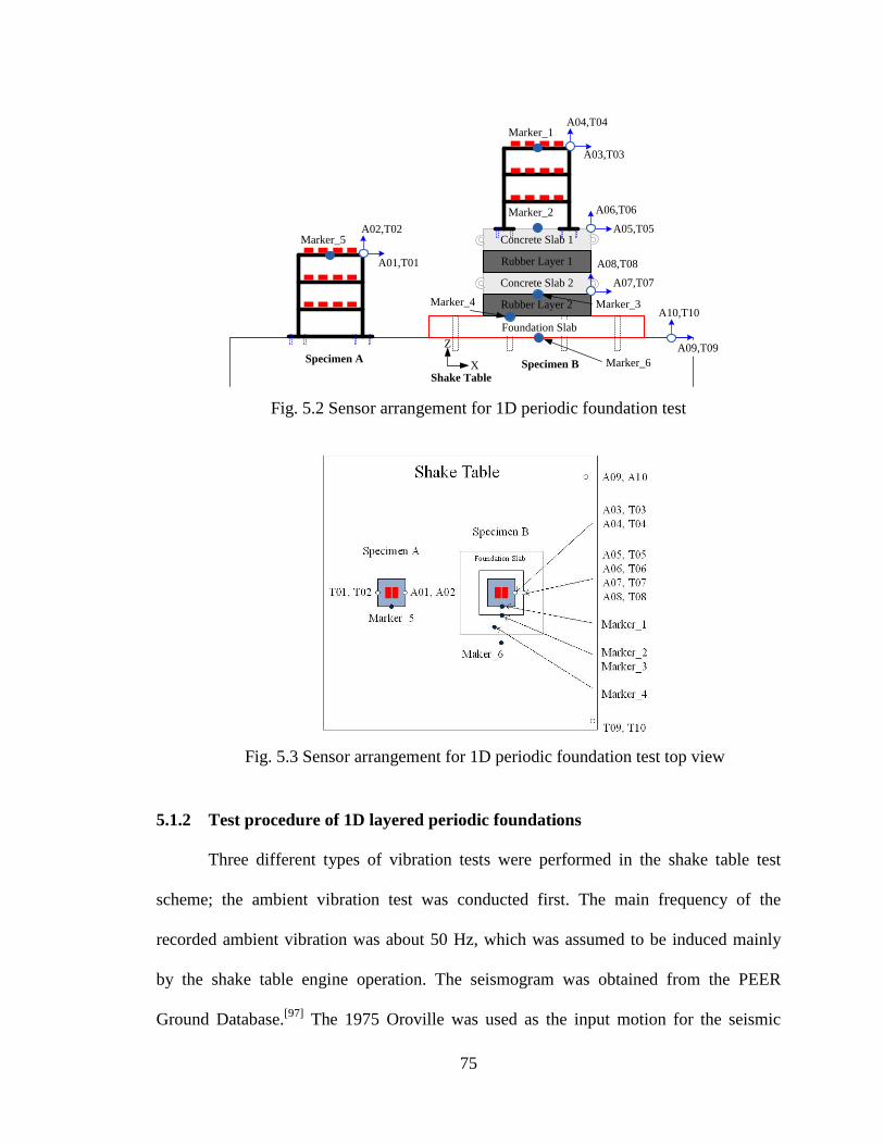
75
5.1.2 Test procedure of 1D layered periodic foundations
Three different types of vibration tests were performed in the shake table test
scheme; the ambient vibration test was conducted first. The main frequency of the
recorded ambient vibration was about 50 Hz, which was assumed to be induced mainly
by the shake table engine operation. The seismogram was obtained from the PEER
Ground Database.[97]
The 1975 Oroville was used as the input motion for the seismic
Fig. 5.2 Sensor arrangement for 1D periodic foundation test
Shake Table
Specimen ASpecimen B
A01,T01
A02,T02
Concrete Slab 2
Concrete Slab 1
Rubber Layer 1
Rubber Layer 2
Foundation Slab
A03,T03
A04,T04
A05,T05
A06,T06
A07,T07
A08,T08
A09,T09
A10,T10
X
Z
Marker_5
Marker_1
Marker_2
Marker_4 Marker_3
Marker_6
Fig. 5.3 Sensor arrangement for 1D periodic foundation test top view
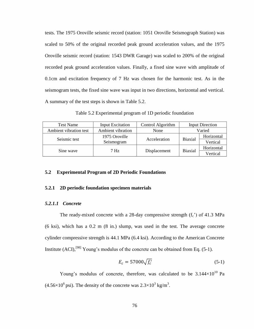
76
tests. The 1975 Oroville seismic record (station: 1051 Oroville Seismograph Station) was
scaled to 50% of the original recorded peak ground acceleration values, and the 1975
Oroville seismic record (station: 1543 DWR Garage) was scaled to 200% of the original
recorded peak ground acceleration values. Finally, a fixed sine wave with amplitude of
0.1cm and excitation frequency of 7 Hz was chosen for the harmonic test. As in the
seismogram tests, the fixed sine wave was input in two directions, horizontal and vertical.
A summary of the test steps is shown in Table 5.2.
Table 5.2 Experimental program of 1D periodic foundation
Test Name Input Excitation Control Algorithm Input Direction
Ambient vibration test Ambient vibration None Varied
Seismic test 1975 Oroville
Seismogram Acceleration Biaxial
Horizontal
Vertical
Sine wave 7 Hz Displacement Biaxial Horizontal
Vertical
5.2 Experimental Program of 2D Periodic Foundations
5.2.1 2D periodic foundation specimen materials
5.2.1.1 Concrete
The ready-mixed concrete with a 28-day compressive strength (fc’) of 41.3 MPa
(6 ksi), which has a 0.2 m (8 in.) slump, was used in the test. The average concrete
cylinder compressive strength is 44.1 MPa (6.4 ksi). According to the American Concrete
Institute (ACI),[98]
Young’s modulus of the concrete can be obtained from Eq. (5-1).
√ (5-1)
Young’s modulus of concrete, therefore, was calculated to be 3.144×10¹⁰
Pa
(4.56×10⁶
psi). The density of the concrete was 2.3×10³ kg/m
3.
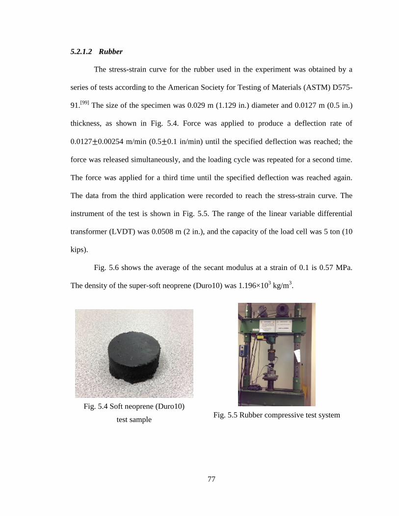
77
5.2.1.2 Rubber
The stress-strain curve for the rubber used in the experiment was obtained by a
series of tests according to the American Society for Testing of Materials (ASTM) D575-
91.[99]
The size of the specimen was 0.029 m (1.129 in.) diameter and 0.0127 m (0.5 in.)
thickness, as shown in Fig. 5.4. Force was applied to produce a deflection rate of
0.0127 0.00254 m/min (0.5 0.1 in/min) until the specified deflection was reached; the
force was released simultaneously, and the loading cycle was repeated for a second time.
The force was applied for a third time until the specified deflection was reached again.
The data from the third application were recorded to reach the stress-strain curve. The
instrument of the test is shown in Fig. 5.5. The range of the linear variable differential
transformer (LVDT) was 0.0508 m (2 in.), and the capacity of the load cell was 5 ton (10
kips).
Fig. 5.6 shows the average of the secant modulus at a strain of 0.1 is 0.57 MPa.
The density of the super-soft neoprene (Duro10) was 1.196×10³ kg/m
3.
Fig. 5.4 Soft neoprene (Duro10)
test sample
Fig. 5.5 Rubber compressive test system
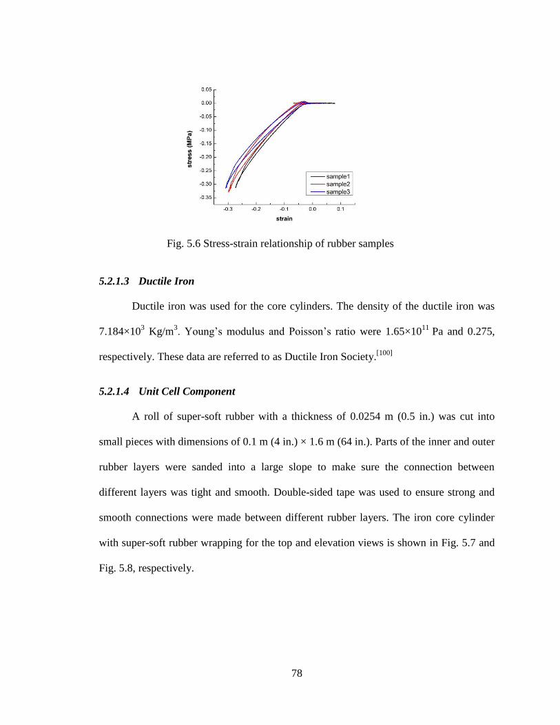
78
5.2.1.3 Ductile Iron
Ductile iron was used for the core cylinders. The density of the ductile iron was
7.184×10³ Kg/m
3. Young’s modulus and Poisson’s ratio were 1.65×10
11 Pa and 0.275,
respectively. These data are referred to as Ductile Iron Society.[100]
5.2.1.4 Unit Cell Component
A roll of super-soft rubber with a thickness of 0.0254 m (0.5 in.) was cut into
small pieces with dimensions of 0.1 m (4 in.) × 1.6 m (64 in.). Parts of the inner and outer
rubber layers were sanded into a large slope to make sure the connection between
different layers was tight and smooth. Double-sided tape was used to ensure strong and
smooth connections were made between different rubber layers. The iron core cylinder
with super-soft rubber wrapping for the top and elevation views is shown in Fig. 5.7 and
Fig. 5.8, respectively.
Fig. 5.6 Stress-strain relationship of rubber samples
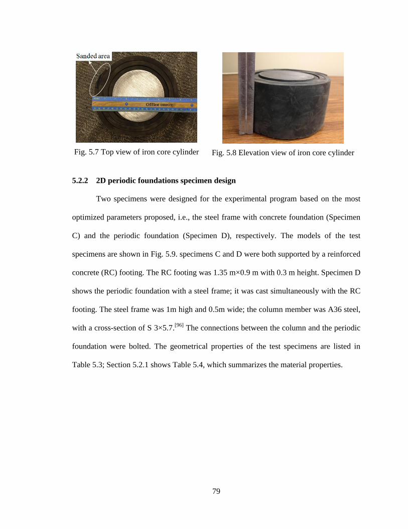
79
5.2.2 2D periodic foundations specimen design
Two specimens were designed for the experimental program based on the most
optimized parameters proposed, i.e., the steel frame with concrete foundation (Specimen
C) and the periodic foundation (Specimen D), respectively. The models of the test
specimens are shown in Fig. 5.9. specimens C and D were both supported by a reinforced
concrete (RC) footing. The RC footing was 1.35 m×0.9 m with 0.3 m height. Specimen D
shows the periodic foundation with a steel frame; it was cast simultaneously with the RC
footing. The steel frame was 1m high and 0.5m wide; the column member was A36 steel,
with a cross-section of S 3×5.7.[96]
The connections between the column and the periodic
foundation were bolted. The geometrical properties of the test specimens are listed in
Table 5.3; Section 5.2.1 shows Table 5.4, which summarizes the material properties.
Fig. 5.7 Top view of iron core cylinder
Fig. 5.8 Elevation view of iron core cylinder

80
Table 5.3 Geometric properties of one unit cell
Item Material Dimension
Core cylinder Ductile cast iron Diameter = 0.12 m.
Rubber coating Supper soft rubber (Duro 10) Outer diameter = 0.2 m.
Matrix Reinforced Concrete Length of unit cell (a) = 0.254 m
Table 5.4 Material properties of 2D periodic foundation specimens
Material Density (kg/m3) Young’s Modulus (Pa) Poisson’s Ratio
Ductile cast iron 7.184×10³ 1.65×10¹¹
0.275
Supper soft rubber 1.196×10³ 5.7×10⁵ 0.463
Steel 7.85×10³ 2.05×10¹¹
0.28
Concrete 2.3×10³ 3.144×10¹⁰
0.33
5.2.2.1 Arrangement of Reinforcement
The reinforcement arrangement in Specimen D is shown in Fig. 5.10 to Fig. 5.11.
The rebar adopted in the periodic foundation was #2 (diameter of 6.35 mm), and the rebar
in the RC base was #5 Grade 60 (diameter of 15.875 mm). Table 5.5 shows the
reinforcement ratio in the 2D periodic foundation and the RC footing, respectively. In
addition, four more steel rebars, i.e., #6 Grade 60 (diameter of 19.05 mm), were applied
Fig. 5.9 Test specimens of 2D periodic foundation tests
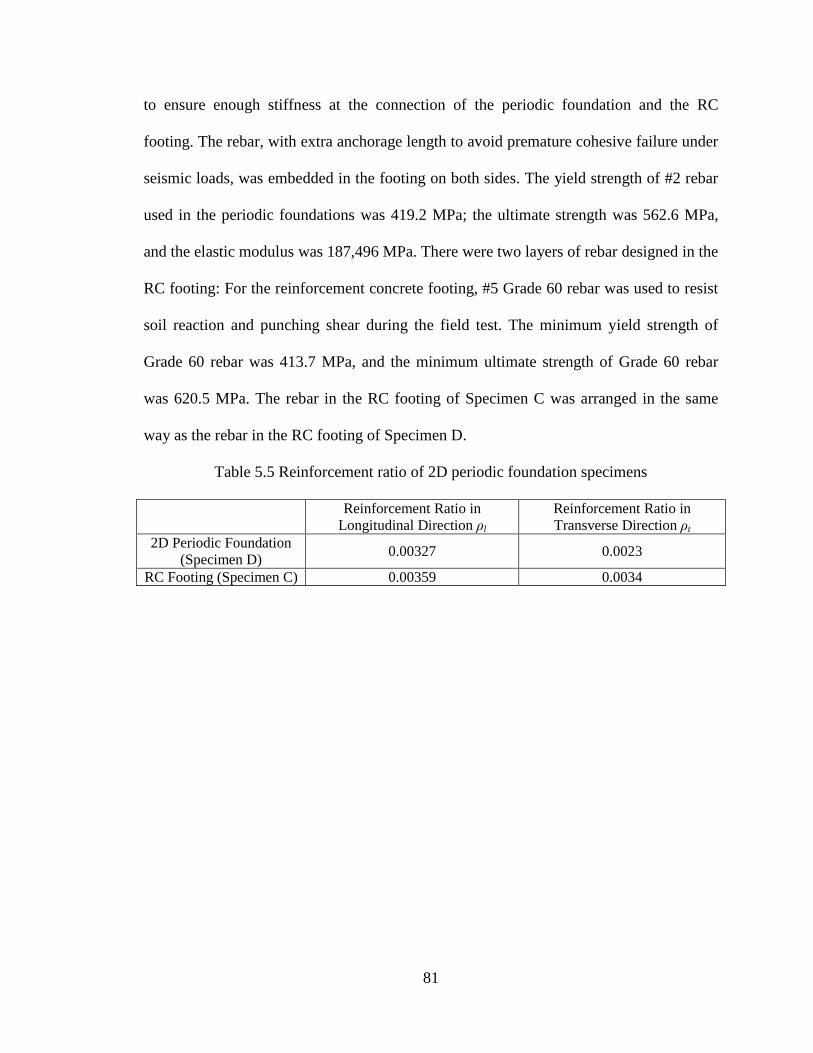
81
to ensure enough stiffness at the connection of the periodic foundation and the RC
footing. The rebar, with extra anchorage length to avoid premature cohesive failure under
seismic loads, was embedded in the footing on both sides. The yield strength of #2 rebar
used in the periodic foundations was 419.2 MPa; the ultimate strength was 562.6 MPa,
and the elastic modulus was 187,496 MPa. There were two layers of rebar designed in the
RC footing: For the reinforcement concrete footing, #5 Grade 60 rebar was used to resist
soil reaction and punching shear during the field test. The minimum yield strength of
Grade 60 rebar was 413.7 MPa, and the minimum ultimate strength of Grade 60 rebar
was 620.5 MPa. The rebar in the RC footing of Specimen C was arranged in the same
way as the rebar in the RC footing of Specimen D.
Table 5.5 Reinforcement ratio of 2D periodic foundation specimens
Reinforcement Ratio in
Longitudinal Direction ρl
Reinforcement Ratio in
Transverse Direction ρt
2D Periodic Foundation
(Specimen D) 0.00327 0.0023
RC Footing (Specimen C) 0.00359 0.0034
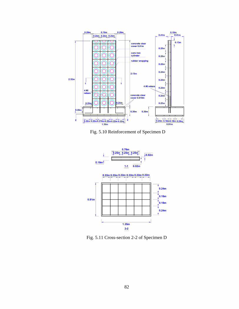
82
Fig. 5.10 Reinforcement of Specimen D
Fig. 5.11 Cross-section 2-2 of Specimen D
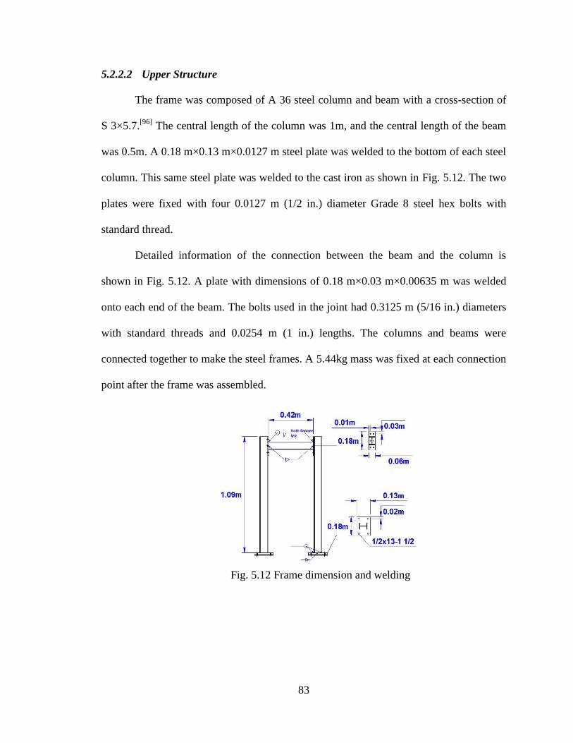
83
5.2.2.2 Upper Structure
The frame was composed of A 36 steel column and beam with a cross-section of
S 3×5.7.[96]
The central length of the column was 1m, and the central length of the beam
was 0.5m. A 0.18 m×0.13 m×0.0127 m steel plate was welded to the bottom of each steel
column. This same steel plate was welded to the cast iron as shown in Fig. 5.12. The two
plates were fixed with four 0.0127 m (1/2 in.) diameter Grade 8 steel hex bolts with
standard thread.
Detailed information of the connection between the beam and the column is
shown in Fig. 5.12. A plate with dimensions of 0.18 m×0.03 m×0.00635 m was welded
onto each end of the beam. The bolts used in the joint had 0.3125 m (5/16 in.) diameters
with standard threads and 0.0254 m (1 in.) lengths. The columns and beams were
connected together to make the steel frames. A 5.44kg mass was fixed at each connection
point after the frame was assembled.
Fig. 5.12 Frame dimension and welding
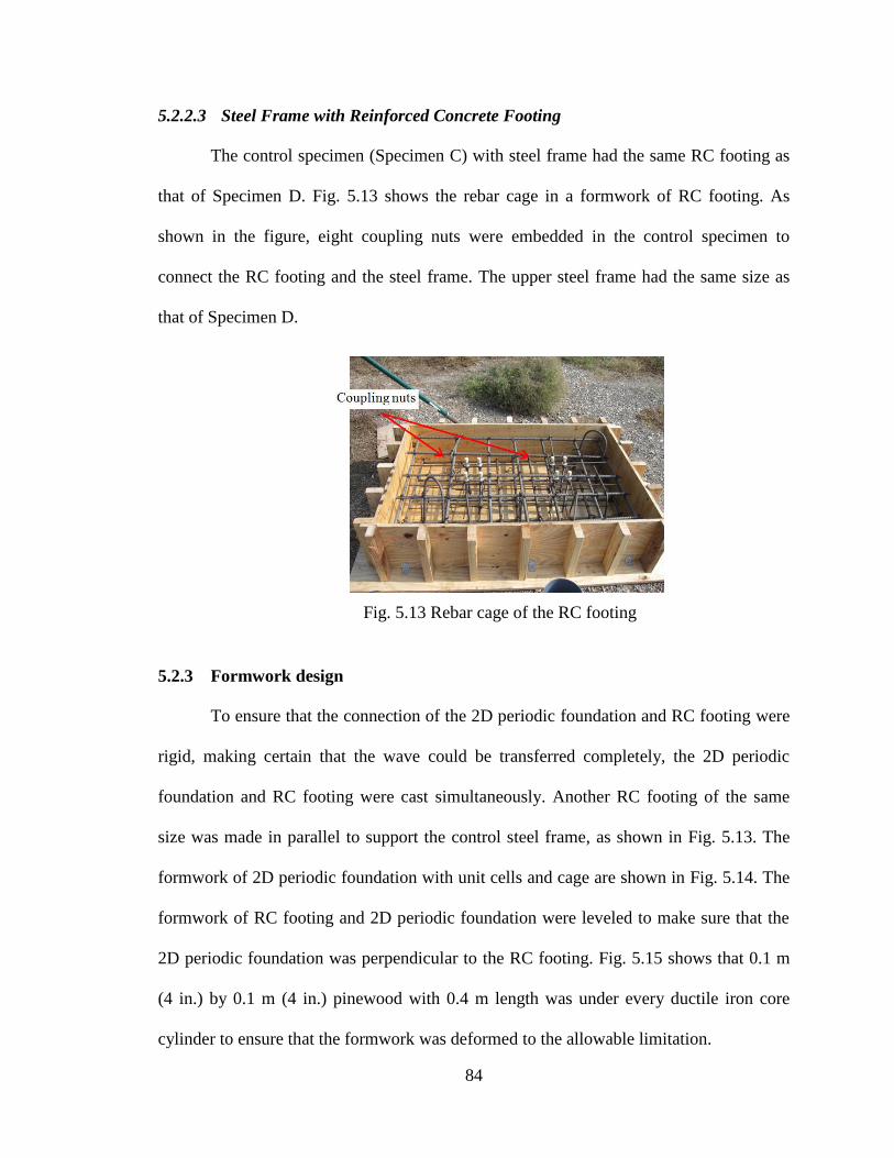
84
5.2.2.3 Steel Frame with Reinforced Concrete Footing
The control specimen (Specimen C) with steel frame had the same RC footing as
that of Specimen D. Fig. 5.13 shows the rebar cage in a formwork of RC footing. As
shown in the figure, eight coupling nuts were embedded in the control specimen to
connect the RC footing and the steel frame. The upper steel frame had the same size as
that of Specimen D.
5.2.3 Formwork design
To ensure that the connection of the 2D periodic foundation and RC footing were
rigid, making certain that the wave could be transferred completely, the 2D periodic
foundation and RC footing were cast simultaneously. Another RC footing of the same
size was made in parallel to support the control steel frame, as shown in Fig. 5.13. The
formwork of 2D periodic foundation with unit cells and cage are shown in Fig. 5.14. The
formwork of RC footing and 2D periodic foundation were leveled to make sure that the
2D periodic foundation was perpendicular to the RC footing. Fig. 5.15 shows that 0.1 m
(4 in.) by 0.1 m (4 in.) pinewood with 0.4 m length was under every ductile iron core
cylinder to ensure that the formwork was deformed to the allowable limitation.
Fig. 5.13 Rebar cage of the RC footing
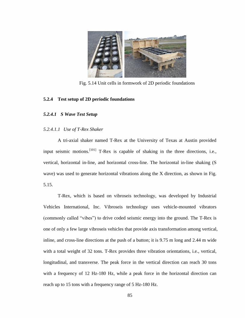
85
5.2.4 Test setup of 2D periodic foundations
5.2.4.1 S Wave Test Setup
5.2.4.1.1 Use of T-Rex Shaker
A tri-axial shaker named T-Rex at the University of Texas at Austin provided
input seismic motions.[101]
T-Rex is capable of shaking in the three directions, i.e.,
vertical, horizontal in-line, and horizontal cross-line. The horizontal in-line shaking (S
wave) was used to generate horizontal vibrations along the X direction, as shown in Fig.
5.15.
T-Rex, which is based on vibroseis technology, was developed by Industrial
Vehicles International, Inc. Vibroseis technology uses vehicle-mounted vibrators
(commonly called “vibes”) to drive coded seismic energy into the ground. The T-Rex is
one of only a few large vibroseis vehicles that provide axis transformation among vertical,
inline, and cross-line directions at the push of a button; it is 9.75 m long and 2.44 m wide
with a total weight of 32 tons. T-Rex provides three vibration orientations, i.e., vertical,
longitudinal, and transverse. The peak force in the vertical direction can reach 30 tons
with a frequency of 12 Hz-180 Hz, while a peak force in the horizontal direction can
reach up to 15 tons with a frequency range of 5 Hz-180 Hz.
Fig. 5.14 Unit cells in formwork of 2D periodic foundations

86
5.2.4.1.2 Use of Rattler Shaker
Rattler was used to generate an S wave to verify the effectiveness of the 2D
periodic foundation. The 3D accelerometers were mounted on the top of the frame on
Specimen C and Specimen D to record the accelerations. The positions of the
accelerometers are marked in Fig. 5.17. The reinforced concrete footing with an upper
steel frame is shown as Specimen C, and the periodic foundation with an upper steel
frame is shown as Specimen D in Fig. 5.17. The input accelerations were provided by
Rattler,[102]
which is 8.7 m long and 2.6 m wide with a total weight of 24,176 kg. Rattler
provides shear waves with a peak force of 133 kN and a frequency from 100 Hz to 5 Hz.
Fig. 5.15 Picture of field test setup using T-Rex
Fig. 5.16 Layout of test setup under S wave excitations using T-Rex
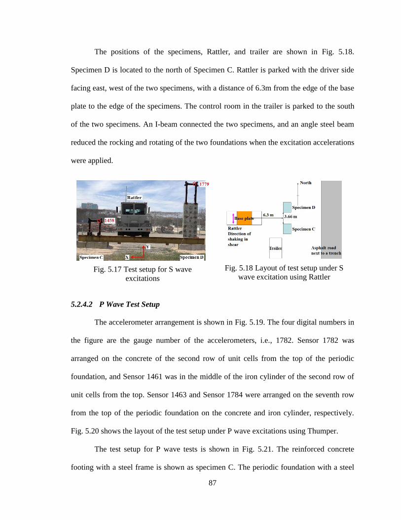
87
The positions of the specimens, Rattler, and trailer are shown in Fig. 5.18.
Specimen D is located to the north of Specimen C. Rattler is parked with the driver side
facing east, west of the two specimens, with a distance of 6.3m from the edge of the base
plate to the edge of the specimens. The control room in the trailer is parked to the south
of the two specimens. An I-beam connected the two specimens, and an angle steel beam
reduced the rocking and rotating of the two foundations when the excitation accelerations
were applied.
5.2.4.2 P Wave Test Setup
The accelerometer arrangement is shown in Fig. 5.19. The four digital numbers in
the figure are the gauge number of the accelerometers, i.e., 1782. Sensor 1782 was
arranged on the concrete of the second row of unit cells from the top of the periodic
foundation, and Sensor 1461 was in the middle of the iron cylinder of the second row of
unit cells from the top. Sensor 1463 and Sensor 1784 were arranged on the seventh row
from the top of the periodic foundation on the concrete and iron cylinder, respectively.
Fig. 5.20 shows the layout of the test setup under P wave excitations using Thumper.
The test setup for P wave tests is shown in Fig. 5.21. The reinforced concrete
footing with a steel frame is shown as specimen C. The periodic foundation with a steel
Fig. 5.17 Test setup for S wave
excitations
Fig. 5.18 Layout of test setup under S
wave excitation using Rattler

88
frame is shown as Specimen D. The shaker, Thumper,[103]
was developed by Industrial
Vehicles International, Inc. Thumper is a high frequency shaker with a capacity of up to
500 Hz. The peak force in the vertical direction can be up to 26.7 kN with a frequency in
the range of 17 Hz to 225 Hz. The shaker provides two vibration orientations in both
vertical and horizontal directions (360 degrees); its length is 8.23 m, and its width is 2.6
m, with a total weight of 11,258 kg.
5.2.5 Test procedure of 2D periodic foundations
Three different types of vibration tests were conducted. Stepped sine wave tests
were first conducted to determine the frequency band gaps of the periodic foundation. A
Fig. 5.19 Accelerometer
arrangement for P wave tests
Fig. 5.20 Layout of test setup under P wave
excitations
Fig. 5.21 Test setup for P wave excitations
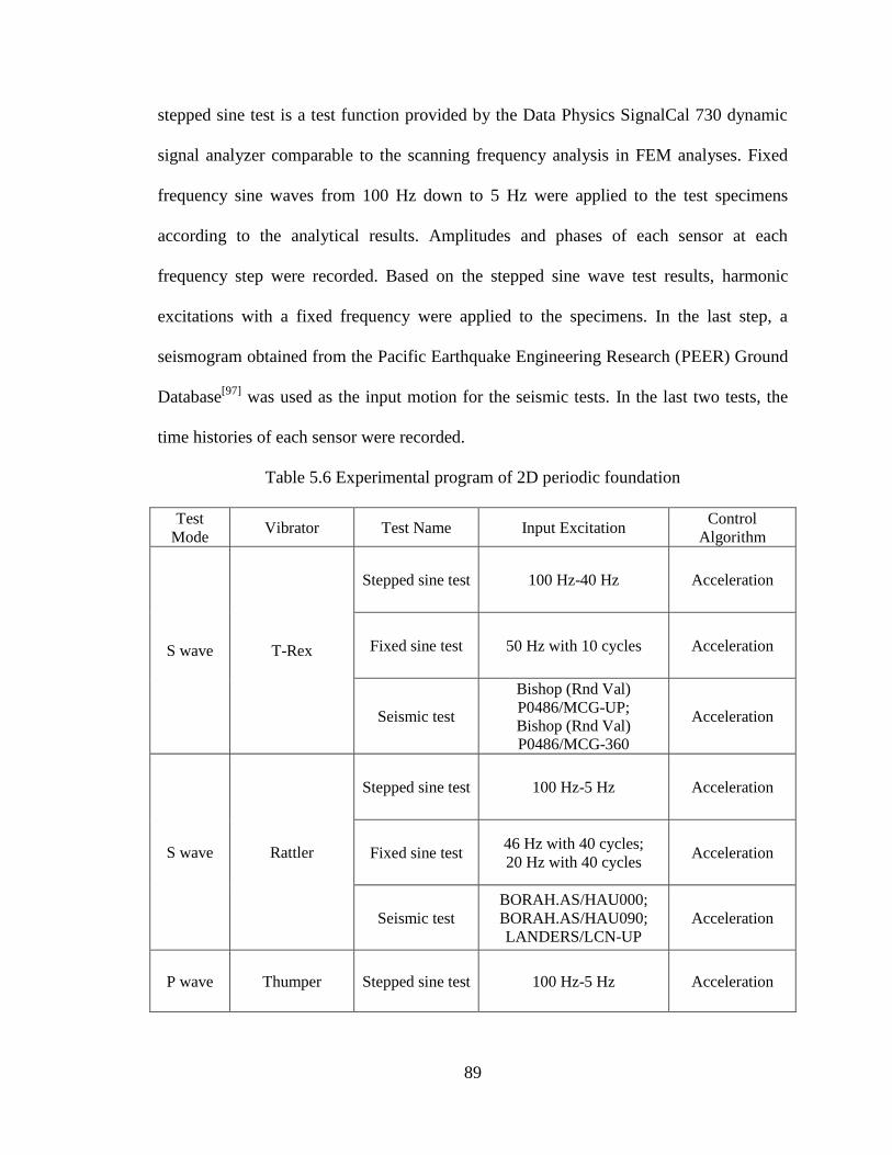
89
stepped sine test is a test function provided by the Data Physics SignalCal 730 dynamic
signal analyzer comparable to the scanning frequency analysis in FEM analyses. Fixed
frequency sine waves from 100 Hz down to 5 Hz were applied to the test specimens
according to the analytical results. Amplitudes and phases of each sensor at each
frequency step were recorded. Based on the stepped sine wave test results, harmonic
excitations with a fixed frequency were applied to the specimens. In the last step, a
seismogram obtained from the Pacific Earthquake Engineering Research (PEER) Ground
Database[97]
was used as the input motion for the seismic tests. In the last two tests, the
time histories of each sensor were recorded.
Table 5.6 Experimental program of 2D periodic foundation
Test
Mode Vibrator Test Name Input Excitation
Control
Algorithm
S wave T-Rex
Stepped sine test 100 Hz-40 Hz Acceleration
Fixed sine test 50 Hz with 10 cycles Acceleration
Seismic test
Bishop (Rnd Val)
P0486/MCG-UP;
Bishop (Rnd Val)
P0486/MCG-360
Acceleration
S wave Rattler
Stepped sine test 100 Hz-5 Hz Acceleration
Fixed sine test 46 Hz with 40 cycles;
20 Hz with 40 cycles Acceleration
Seismic test
BORAH.AS/HAU000;
BORAH.AS/HAU090;
LANDERS/LCN-UP
Acceleration
P wave Thumper Stepped sine test 100 Hz-5 Hz Acceleration
90
Fixed sine test 72.6 Hz with 40 cycles;
36 Hz with 40 cycles Acceleration
Seismic test
Bishop (Rnd Val)
P0486/MCG-UP ;
Bishop (Rnd Val)
P0486/MCG-360
Acceleration
5.3 Experimental Program of 3D Periodic Foundations
5.3.1 3D periodic foundation specimen materials
5.3.1.1 Concrete
The ready mixed concrete had a 28-day compressive strength (fc’) of 6 ksi. Nine
standard cylinders, with the dimension of 152 mm×305 mm (6 in.×12 in.) were cast along
with the specimens. The cylinders were cured under the same conditions as the test
specimens. The standard cylinders were under a moist environment covered by a plastic
sheet for the first seven days. The cylinders were tested the same day as the field test was
conducted. The average concrete cylinder compressive strength is 55.8 MPa (8.1 ksi);
Young’s modulus of concrete is calculated as 5.67×10⁶ psi (4.0×10
10 Pa); the density of
the concrete is 2.3×10³ kg/m
3.
5.3.1.2 Ultra-Soft Polyurethane
The Young’s modulus of the wrapping rubber is an important parameter on the
starting frequency band gap. According to the previous analysis in Section 4.3.1.1, a
lower Young’s modulus will provide a lower starting frequency and smaller bandwidth
than the first band gap. To get a lower Young’s modulus, ultra-soft polyurethane is used
as the wrapping coat for the 3D periodic foundation specimen. This nonporous material,
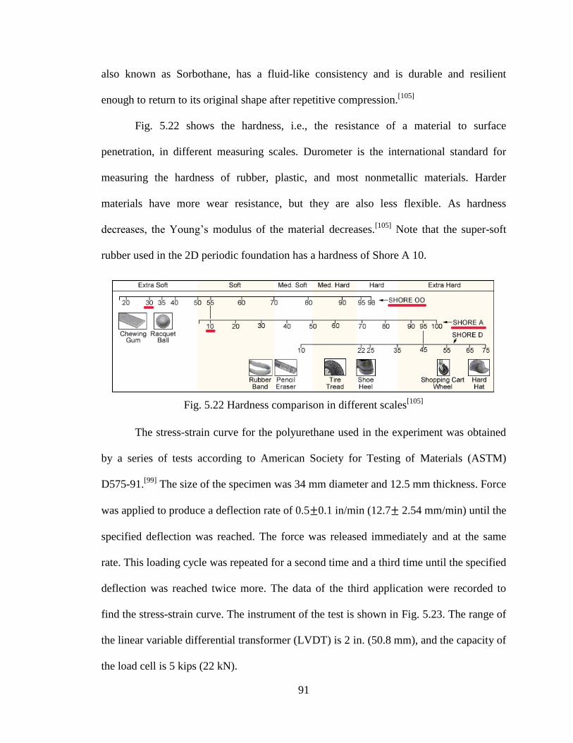
91
also known as Sorbothane, has a fluid-like consistency and is durable and resilient
enough to return to its original shape after repetitive compression.[105]
Fig. 5.22 shows the hardness, i.e., the resistance of a material to surface
penetration, in different measuring scales. Durometer is the international standard for
measuring the hardness of rubber, plastic, and most nonmetallic materials. Harder
materials have more wear resistance, but they are also less flexible. As hardness
decreases, the Young’s modulus of the material decreases.[105]
Note that the super-soft
rubber used in the 2D periodic foundation has a hardness of Shore A 10.
The stress-strain curve for the polyurethane used in the experiment was obtained
by a series of tests according to American Society for Testing of Materials (ASTM)
D575-91.[99]
The size of the specimen was 34 mm diameter and 12.5 mm thickness. Force
was applied to produce a deflection rate of 0.5 0.1 in/min (12.7 2.54 mm/min) until the
specified deflection was reached. The force was released immediately and at the same
rate. This loading cycle was repeated for a second time and a third time until the specified
deflection was reached twice more. The data of the third application were recorded to
find the stress-strain curve. The instrument of the test is shown in Fig. 5.23. The range of
the linear variable differential transformer (LVDT) is 2 in. (50.8 mm), and the capacity of
the load cell is 5 kips (22 kN).
Fig. 5.22 Hardness comparison in different scales[105]

92
Fig. 5.24 shows that the average of the secant modulus for Oo 30 at a strain of -
0.1 is 0.1586 MPa is smaller than Oo40 and Oo 70 polyurethane and also smaller than the
A 10 super-soft rubber used in the 2D periodic foundation. The density of the ultra-soft
polyurethane is 1.277×10³ kg/m
3. Tensile Strength of Oo 30 is 83 psi (0.572 MPa), and
the mechanical properties of Oo 30 are valid in a temperature range of 0° to 160° F.
Fig. 5.23 Ultra-soft polyurethane compression test setup
Fig. 5.24 Stress-strain relationship for polyurethane and rubber
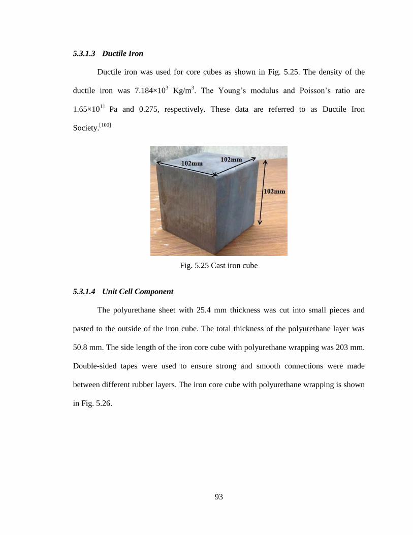
93
5.3.1.3 Ductile Iron
Ductile iron was used for core cubes as shown in Fig. 5.25. The density of the
ductile iron was 7.184×10³ Kg/m
3. The Young’s modulus and Poisson’s ratio are
1.65×10¹¹
Pa and 0.275, respectively. These data are referred to as Ductile Iron
Society.[100]
5.3.1.4 Unit Cell Component
The polyurethane sheet with 25.4 mm thickness was cut into small pieces and
pasted to the outside of the iron cube. The total thickness of the polyurethane layer was
50.8 mm. The side length of the iron core cube with polyurethane wrapping was 203 mm.
Double-sided tapes were used to ensure strong and smooth connections were made
between different rubber layers. The iron core cube with polyurethane wrapping is shown
in Fig. 5.26.
Fig. 5.25 Cast iron cube
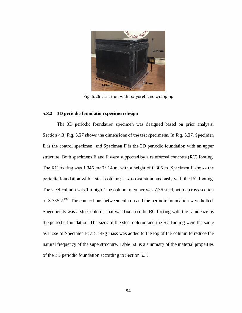
94
5.3.2 3D periodic foundation specimen design
The 3D periodic foundation specimen was designed based on prior analysis,
Section 4.3; Fig. 5.27 shows the dimensions of the test specimens. In Fig. 5.27, Specimen
E is the control specimen, and Specimen F is the 3D periodic foundation with an upper
structure. Both specimens E and F were supported by a reinforced concrete (RC) footing.
The RC footing was 1.346 m×0.914 m, with a height of 0.305 m. Specimen F shows the
periodic foundation with a steel column; it was cast simultaneously with the RC footing.
The steel column was 1m high. The column member was A36 steel, with a cross-section
of S 3×5.7.[96]
The connections between column and the periodic foundation were bolted.
Specimen E was a steel column that was fixed on the RC footing with the same size as
the periodic foundation. The sizes of the steel column and the RC footing were the same
as those of Specimen F; a 5.44kg mass was added to the top of the column to reduce the
natural frequency of the superstructure. Table 5.8 is a summary of the material properties
of the 3D periodic foundation according to Section 5.3.1
Fig. 5.26 Cast iron with polyurethane wrapping
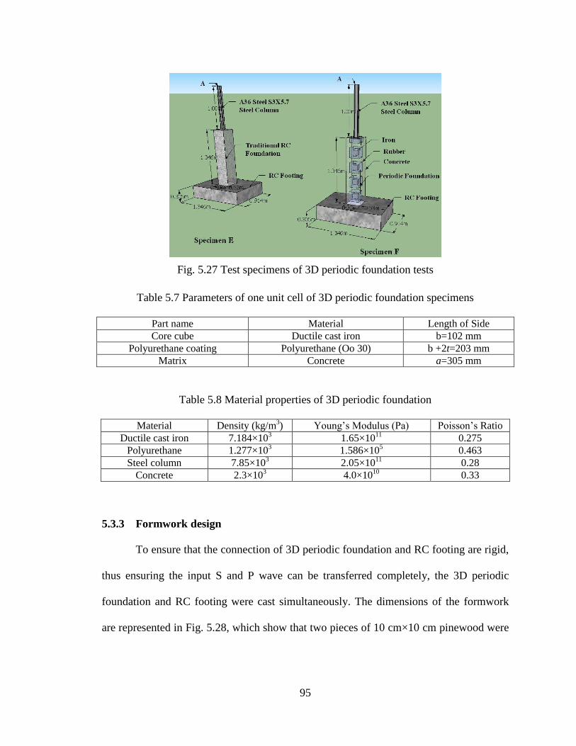
95
Table 5.7 Parameters of one unit cell of 3D periodic foundation specimens
Part name Material Length of Side
Core cube Ductile cast iron b=102 mm
Polyurethane coating Polyurethane (Oo 30) b +2t=203 mm
Matrix Concrete a=305 mm
Table 5.8 Material properties of 3D periodic foundation
Material Density (kg/m3) Young’s Modulus (Pa) Poisson’s Ratio
Ductile cast iron 7.184×10³ 1.65×10
11 0.275
Polyurethane 1.277×10³ 1.586×10
5 0.463
Steel column 7.85×10³ 2.05×10
11 0.28
Concrete 2.3×10³ 4.0×10
10 0.33
5.3.3 Formwork design
To ensure that the connection of 3D periodic foundation and RC footing are rigid,
thus ensuring the input S and P wave can be transferred completely, the 3D periodic
foundation and RC footing were cast simultaneously. The dimensions of the formwork
are represented in Fig. 5.28, which show that two pieces of 10 cm×10 cm pinewood were
Fig. 5.27 Test specimens of 3D periodic foundation tests
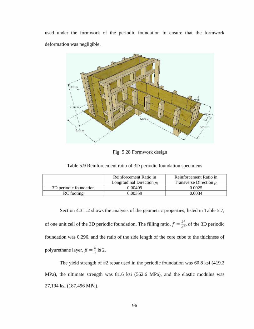
96
used under the formwork of the periodic foundation to ensure that the formwork
deformation was negligible.
Table 5.9 Reinforcement ratio of 3D periodic foundation specimens
Reinforcement Ratio in
Longitudinal Direction ρl
Reinforcement Ratio in
Transverse Direction ρt
3D periodic foundation 0.00409 0.0025
RC footing 0.00359 0.0034
Section 4.3.1.2 shows the analysis of the geometric properties, listed in Table 5.7,
of one unit cell of the 3D periodic foundation. The filling ratio,
, of the 3D periodic
foundation was 0.296, and the ratio of the side length of the core cube to the thickness of
polyurethane layer,
is 2.
The yield strength of #2 rebar used in the periodic foundation was 60.8 ksi (419.2
MPa), the ultimate strength was 81.6 ksi (562.6 MPa), and the elastic modulus was
27,194 ksi (187,496 MPa).
Fig. 5.28 Formwork design
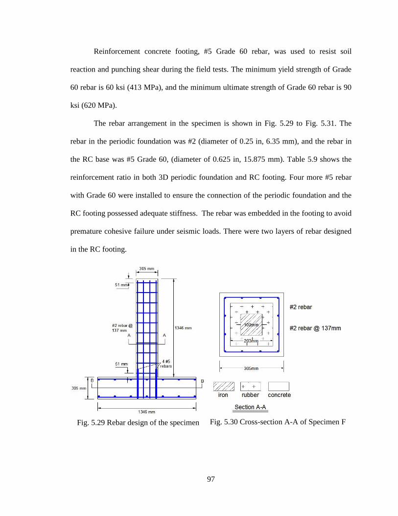
97
Reinforcement concrete footing, #5 Grade 60 rebar, was used to resist soil
reaction and punching shear during the field tests. The minimum yield strength of Grade
60 rebar is 60 ksi (413 MPa), and the minimum ultimate strength of Grade 60 rebar is 90
ksi (620 MPa).
The rebar arrangement in the specimen is shown in Fig. 5.29 to Fig. 5.31. The
rebar in the periodic foundation was #2 (diameter of 0.25 in, 6.35 mm), and the rebar in
the RC base was #5 Grade 60, (diameter of 0.625 in, 15.875 mm). Table 5.9 shows the
reinforcement ratio in both 3D periodic foundation and RC footing. Four more #5 rebar
with Grade 60 were installed to ensure the connection of the periodic foundation and the
RC footing possessed adequate stiffness. The rebar was embedded in the footing to avoid
premature cohesive failure under seismic loads. There were two layers of rebar designed
in the RC footing.
Fig. 5.29 Rebar design of the specimen
Fig. 5.30 Cross-section A-A of Specimen F
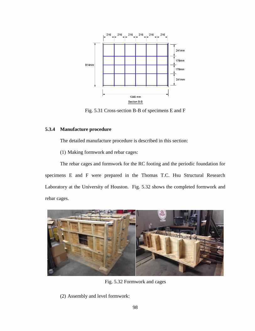
98
5.3.4 Manufacture procedure
The detailed manufacture procedure is described in this section:
(1) Making formwork and rebar cages:
The rebar cages and formwork for the RC footing and the periodic foundation for
specimens E and F were prepared in the Thomas T.C. Hsu Structural Research
Laboratory at the University of Houston. Fig. 5.32 shows the completed formwork and
rebar cages.
(2) Assembly and level formwork:
Fig. 5.31 Cross-section B-B of specimens E and F
Fig. 5.32 Formwork and cages
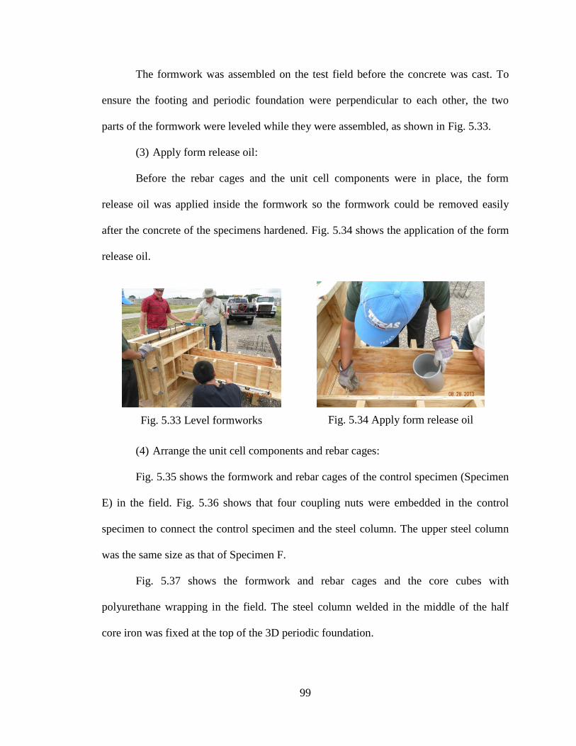
99
The formwork was assembled on the test field before the concrete was cast. To
ensure the footing and periodic foundation were perpendicular to each other, the two
parts of the formwork were leveled while they were assembled, as shown in Fig. 5.33.
(3) Apply form release oil:
Before the rebar cages and the unit cell components were in place, the form
release oil was applied inside the formwork so the formwork could be removed easily
after the concrete of the specimens hardened. Fig. 5.34 shows the application of the form
release oil.
(4) Arrange the unit cell components and rebar cages:
Fig. 5.35 shows the formwork and rebar cages of the control specimen (Specimen
E) in the field. Fig. 5.36 shows that four coupling nuts were embedded in the control
specimen to connect the control specimen and the steel column. The upper steel column
was the same size as that of Specimen F.
Fig. 5.37 shows the formwork and rebar cages and the core cubes with
polyurethane wrapping in the field. The steel column welded in the middle of the half
core iron was fixed at the top of the 3D periodic foundation.
Fig. 5.33 Level formworks
Fig. 5.34 Apply form release oil
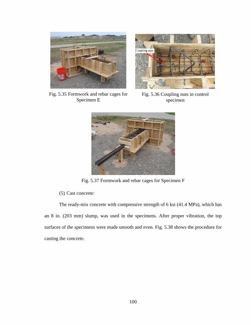
100
(5) Cast concrete:
The ready-mix concrete with compressive strength of 6 ksi (41.4 MPa), which has
an 8 in. (203 mm) slump, was used in the specimens. After proper vibration, the top
surfaces of the specimens were made smooth and even. Fig. 5.38 shows the procedure for
casting the concrete.
Fig. 5.35 Formwork and rebar cages for
Specimen E
Fig. 5.36 Coupling nuts in control
specimen
Fig. 5.37 Formwork and rebar cages for Specimen F
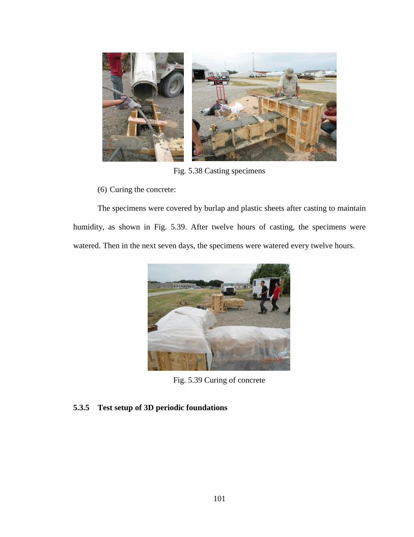
101
(6) Curing the concrete:
The specimens were covered by burlap and plastic sheets after casting to maintain
humidity, as shown in Fig. 5.39. After twelve hours of casting, the specimens were
watered. Then in the next seven days, the specimens were watered every twelve hours.
5.3.5 Test setup of 3D periodic foundations
Fig. 5.38 Casting specimens
Fig. 5.39 Curing of concrete
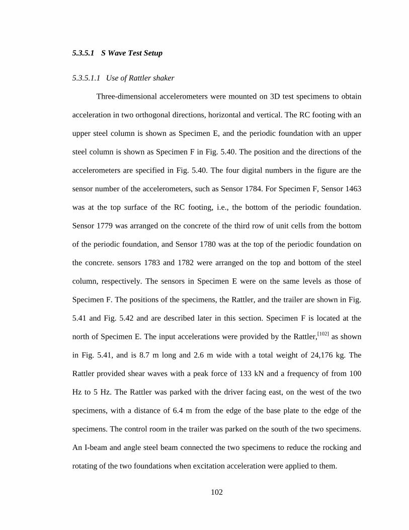
102
5.3.5.1 S Wave Test Setup
5.3.5.1.1 Use of Rattler shaker
Three-dimensional accelerometers were mounted on 3D test specimens to obtain
acceleration in two orthogonal directions, horizontal and vertical. The RC footing with an
upper steel column is shown as Specimen E, and the periodic foundation with an upper
steel column is shown as Specimen F in Fig. 5.40. The position and the directions of the
accelerometers are specified in Fig. 5.40. The four digital numbers in the figure are the
sensor number of the accelerometers, such as Sensor 1784. For Specimen F, Sensor 1463
was at the top surface of the RC footing, i.e., the bottom of the periodic foundation.
Sensor 1779 was arranged on the concrete of the third row of unit cells from the bottom
of the periodic foundation, and Sensor 1780 was at the top of the periodic foundation on
the concrete. sensors 1783 and 1782 were arranged on the top and bottom of the steel
column, respectively. The sensors in Specimen E were on the same levels as those of
Specimen F. The positions of the specimens, the Rattler, and the trailer are shown in Fig.
5.41 and Fig. 5.42 and are described later in this section. Specimen F is located at the
north of Specimen E. The input accelerations were provided by the Rattler,[102]
as shown
in Fig. 5.41, and is 8.7 m long and 2.6 m wide with a total weight of 24,176 kg. The
Rattler provided shear waves with a peak force of 133 kN and a frequency of from 100
Hz to 5 Hz. The Rattler was parked with the driver facing east, on the west of the two
specimens, with a distance of 6.4 m from the edge of the base plate to the edge of the
specimens. The control room in the trailer was parked on the south of the two specimens.
An I-beam and angle steel beam connected the two specimens to reduce the rocking and
rotating of the two foundations when excitation acceleration were applied to them.
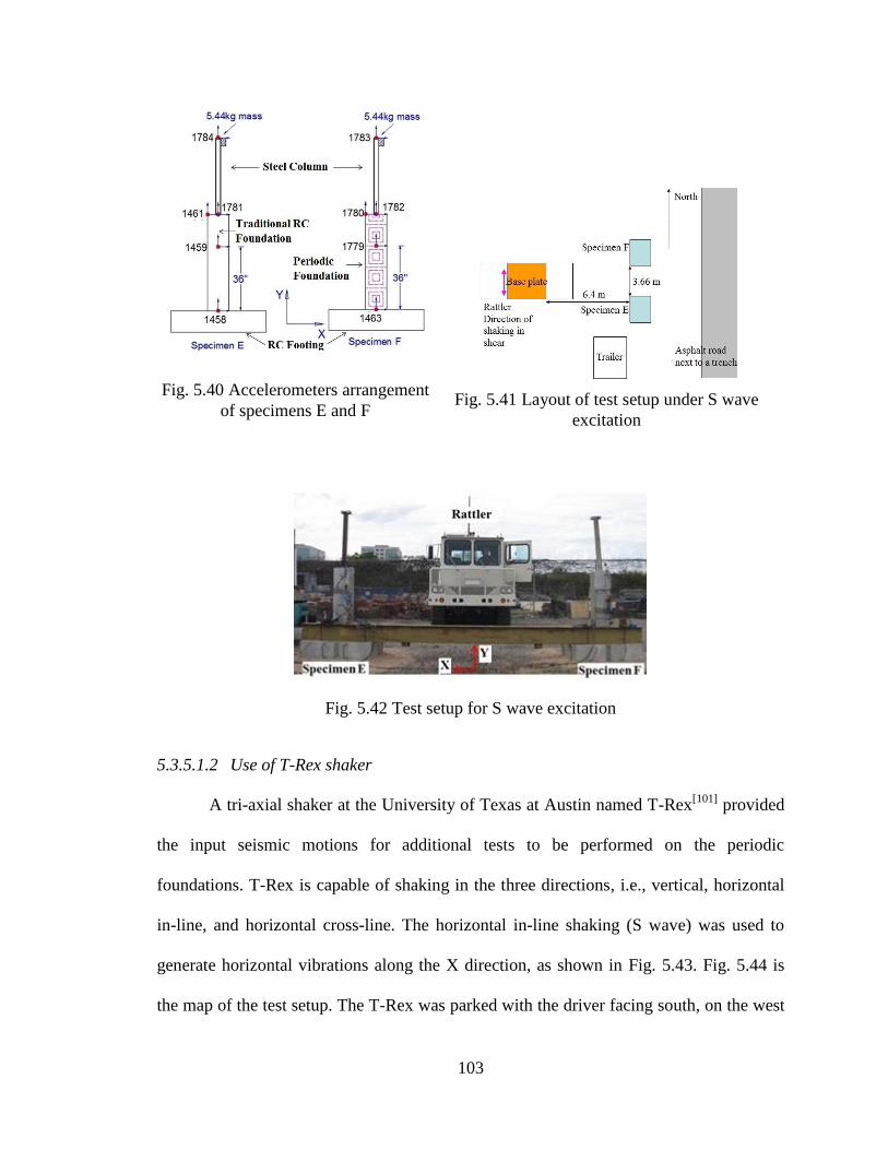
103
5.3.5.1.2 Use of T-Rex shaker
A tri-axial shaker at the University of Texas at Austin named T-Rex[101]
provided
the input seismic motions for additional tests to be performed on the periodic
foundations. T-Rex is capable of shaking in the three directions, i.e., vertical, horizontal
in-line, and horizontal cross-line. The horizontal in-line shaking (S wave) was used to
generate horizontal vibrations along the X direction, as shown in Fig. 5.43. Fig. 5.44 is
the map of the test setup. The T-Rex was parked with the driver facing south, on the west
Fig. 5.40 Accelerometers arrangement
of specimens E and F
Fig. 5.41 Layout of test setup under S wave
excitation
Fig. 5.42 Test setup for S wave excitation
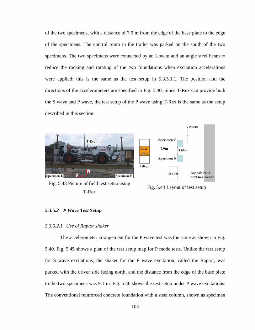
104
of the two specimens, with a distance of 7.9 m from the edge of the base plate to the edge
of the specimens. The control room in the trailer was parked on the south of the two
specimens. The two specimens were connected by an I-beam and an angle steel beam to
reduce the rocking and rotating of the two foundations when excitation accelerations
were applied; this is the same as the test setup in 5.3.5.1.1. The position and the
directions of the accelerometers are specified in Fig. 5.40. Since T-Rex can provide both
the S wave and P wave, the test setup of the P wave using T-Rex is the same as the setup
described in this section.
5.3.5.2 P Wave Test Setup
5.3.5.2.1 Use of Raptor shaker
The accelerometer arrangement for the P wave test was the same as shown in Fig.
5.40. Fig. 5.45 shows a plan of the test setup map for P mode tests. Unlike the test setup
for S wave excitations, the shaker for the P wave excitation, called the Raptor, was
parked with the driver side facing north, and the distance from the edge of the base plate
to the two specimens was 9.1 m. Fig. 5.46 shows the test setup under P wave excitations.
The conventional reinforced concrete foundation with a steel column, shown as specimen
Fig. 5.43 Picture of field test setup using
T-Rex
Fig. 5.44 Layout of test setup
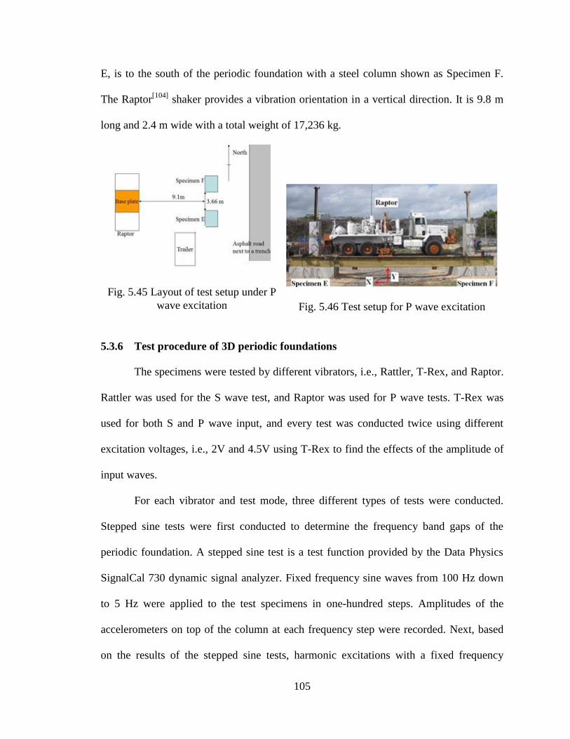
105
E, is to the south of the periodic foundation with a steel column shown as Specimen F.
The Raptor[104]
shaker provides a vibration orientation in a vertical direction. It is 9.8 m
long and 2.4 m wide with a total weight of 17,236 kg.
5.3.6 Test procedure of 3D periodic foundations
The specimens were tested by different vibrators, i.e., Rattler, T-Rex, and Raptor.
Rattler was used for the S wave test, and Raptor was used for P wave tests. T-Rex was
used for both S and P wave input, and every test was conducted twice using different
excitation voltages, i.e., 2V and 4.5V using T-Rex to find the effects of the amplitude of
input waves.
For each vibrator and test mode, three different types of tests were conducted.
Stepped sine tests were first conducted to determine the frequency band gaps of the
periodic foundation. A stepped sine test is a test function provided by the Data Physics
SignalCal 730 dynamic signal analyzer. Fixed frequency sine waves from 100 Hz down
to 5 Hz were applied to the test specimens in one-hundred steps. Amplitudes of the
accelerometers on top of the column at each frequency step were recorded. Next, based
on the results of the stepped sine tests, harmonic excitations with a fixed frequency
Fig. 5.45 Layout of test setup under P
wave excitation
Fig. 5.46 Test setup for P wave excitation
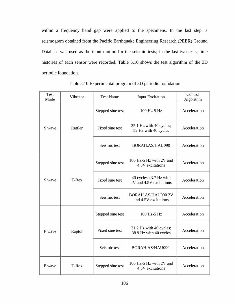
106
within a frequency band gap were applied to the specimens. In the last step, a
seismogram obtained from the Pacific Earthquake Engineering Research (PEER) Ground
Database was used as the input motion for the seismic tests; in the last two tests, time
histories of each sensor were recorded. Table 5.10 shows the test algorithm of the 3D
periodic foundation.
Table 5.10 Experimental program of 3D periodic foundation
Test
Mode Vibrator Test Name Input Excitation
Control
Algorithm
S wave Rattler
Stepped sine test 100 Hz-5 Hz Acceleration
Fixed sine test 35.1 Hz with 40 cycles;
52 Hz with 40 cycles Acceleration
Seismic test BORAH.AS/HAU090 Acceleration
S wave T-Rex
Stepped sine test 100 Hz-5 Hz with 2V and
4.5V excitations Acceleration
Fixed sine test 40 cycles 43.7 Hz with
2V and 4.5V excitations Acceleration
Seismic test BORAH.AS/HAU000 2V
and 4.5V excitations Acceleration
P wave Raptor
Stepped sine test 100 Hz-5 Hz Acceleration
Fixed sine test 21.2 Hz with 40 cycles;
38.9 Hz with 40 cycles Acceleration
Seismic test BORAH.AS/HAU090; Acceleration
P wave T-Rex Stepped sine test 100 Hz-5 Hz with 2V and
4.5V excitations Acceleration
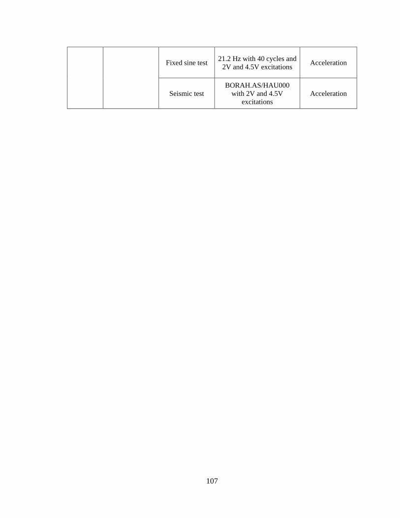
107
Fixed sine test 21.2 Hz with 40 cycles and
2V and 4.5V excitations Acceleration
Seismic test
BORAH.AS/HAU000
with 2V and 4.5V
excitations
Acceleration

109
6 EXPERIMENTAL RESULTS
6.1 Experimental Results of 1D Layered Periodic Foundations
Test results for three test steps are illustrated in this section, i.e., ambient vibration,
the seismic test, and the harmonic test. The shaking table that was used had six degree of
freedom to simulate earthquake motion in three directions. The tested waves were applied
in both horizontal and vertical directions for the seismic test.
6.1.1 Ambient vibration test results
Fig. 6.1 shows acceleration in the horizontal direction on top of the frame with
ambient vibration, caused by the machine with a main frequency of 50 Hz, which is
located in the third attenuation zone as shown in Fig. 4.18. The acceleration on top of the
frame without a foundation (Specimen A) in the horizontal direction is shown as a dashed
gray curve in Fig. 6.1. The red solid curve is the acceleration on top of the frame with a
1D layered periodic foundation in the horizontal direction. The peak acceleration on top
of the frame with a 1D layered periodic foundation (Specimen B) is reduced significantly
compared to that of the frame without the foundation (Specimen A).
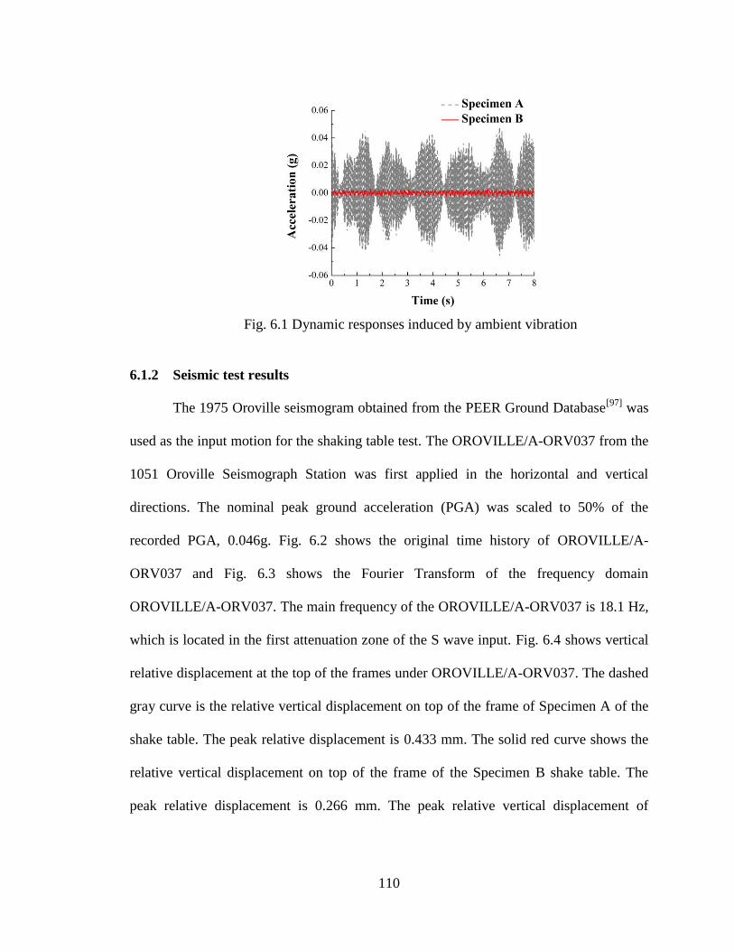
110
6.1.2 Seismic test results
The 1975 Oroville seismogram obtained from the PEER Ground Database[97]
was
used as the input motion for the shaking table test. The OROVILLE/A-ORV037 from the
1051 Oroville Seismograph Station was first applied in the horizontal and vertical
directions. The nominal peak ground acceleration (PGA) was scaled to 50% of the
recorded PGA, 0.046g. Fig. 6.2 shows the original time history of OROVILLE/A-
ORV037 and Fig. 6.3 shows the Fourier Transform of the frequency domain
OROVILLE/A-ORV037. The main frequency of the OROVILLE/A-ORV037 is 18.1 Hz,
which is located in the first attenuation zone of the S wave input. Fig. 6.4 shows vertical
relative displacement at the top of the frames under OROVILLE/A-ORV037. The dashed
gray curve is the relative vertical displacement on top of the frame of Specimen A of the
shake table. The peak relative displacement is 0.433 mm. The solid red curve shows the
relative vertical displacement on top of the frame of the Specimen B shake table. The
peak relative displacement is 0.266 mm. The peak relative vertical displacement of
Fig. 6.1 Dynamic responses induced by ambient vibration
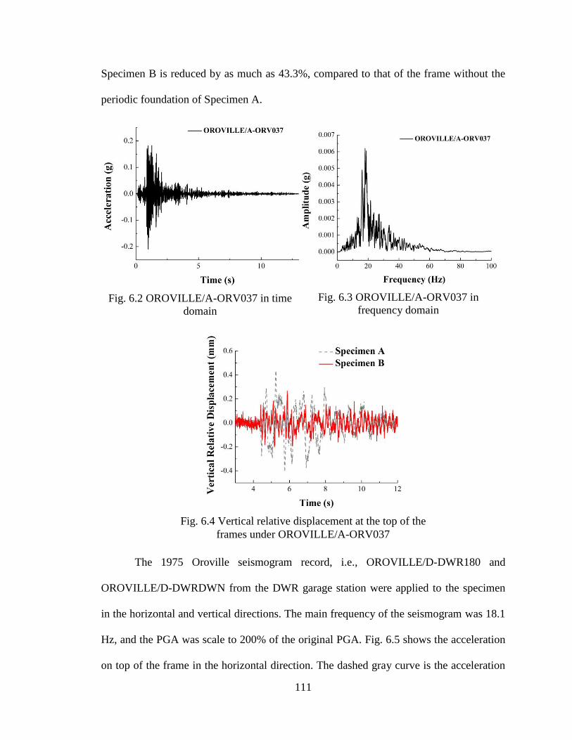
111
Specimen B is reduced by as much as 43.3%, compared to that of the frame without the
periodic foundation of Specimen A.
The 1975 Oroville seismogram record, i.e., OROVILLE/D-DWR180 and
OROVILLE/D-DWRDWN from the DWR garage station were applied to the specimen
in the horizontal and vertical directions. The main frequency of the seismogram was 18.1
Hz, and the PGA was scale to 200% of the original PGA. Fig. 6.5 shows the acceleration
on top of the frame in the horizontal direction. The dashed gray curve is the acceleration
Fig. 6.2 OROVILLE/A-ORV037 in time
domain
Fig. 6.3 OROVILLE/A-ORV037 in
frequency domain
Fig. 6.4 Vertical relative displacement at the top of the
frames under OROVILLE/A-ORV037
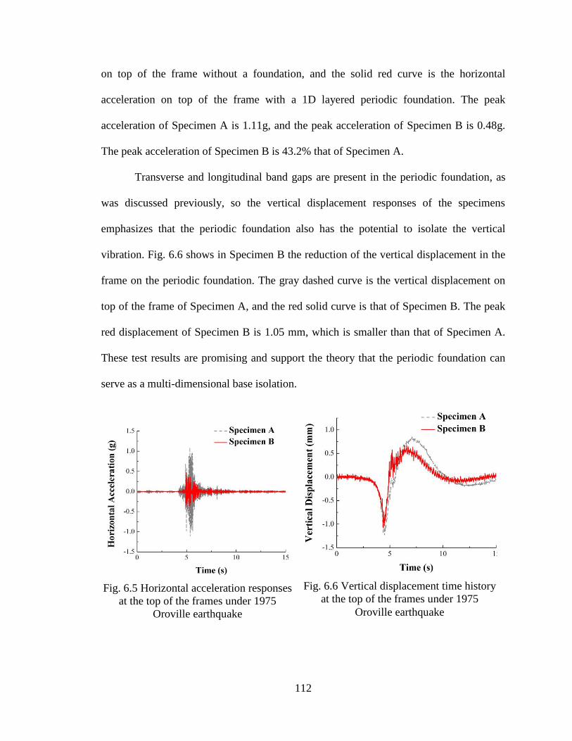
112
on top of the frame without a foundation, and the solid red curve is the horizontal
acceleration on top of the frame with a 1D layered periodic foundation. The peak
acceleration of Specimen A is 1.11g, and the peak acceleration of Specimen B is 0.48g.
The peak acceleration of Specimen B is 43.2% that of Specimen A.
Transverse and longitudinal band gaps are present in the periodic foundation, as
was discussed previously, so the vertical displacement responses of the specimens
emphasizes that the periodic foundation also has the potential to isolate the vertical
vibration. Fig. 6.6 shows in Specimen B the reduction of the vertical displacement in the
frame on the periodic foundation. The gray dashed curve is the vertical displacement on
top of the frame of Specimen A, and the red solid curve is that of Specimen B. The peak
red displacement of Specimen B is 1.05 mm, which is smaller than that of Specimen A.
These test results are promising and support the theory that the periodic foundation can
serve as a multi-dimensional base isolation.
Fig. 6.5 Horizontal acceleration responses
at the top of the frames under 1975
Oroville earthquake
Fig. 6.6 Vertical displacement time history
at the top of the frames under 1975
Oroville earthquake
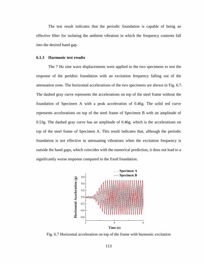
113
The test result indicates that the periodic foundation is capable of being an
effective filter for isolating the ambient vibration in which the frequency contents fall
into the desired band gap.
6.1.3 Harmonic test results
The 7 Hz sine wave displacements were applied to the two specimens to test the
response of the peridoic foundation with an excitation frequency falling out of the
attenuation zone. The horizontal accelerations of the two specimens are shown in Fig. 6.7.
The dashed gray curve represents the accelerations on top of the steel frame without the
foundation of Specimen A with a peak acceleration of 0.46g. The solid red curve
represents accelerations on top of the steel frame of Specimen B with an amplitude of
0.53g. The dashed gray curve has an amplitude of 0.46g, which is the accelerations on
top of the steel frame of Specimen A. This result indicates that, although the periodic
foundation is not effective in attenuating vibrations when the excitation frequency is
outside the band gaps, which coincides with the numerical prediction, it does not lead to a
significantly worse response compared to the fixed foundation.
Fig. 6.7 Horizontal acceleration on top of the frame with harmonic excitation
114
6.2 Experimental Results of 2D Periodic Foundations
The dynamic responses of the 2D periodic foundation tests are covered in this
section. The test results with S wave excitations are presented first. Two vibrators, T-Rex
and Rattler, were used to input S waves. Then, the vibrator called Thumper, was used to
apply the P wave to the specimens; the test results are illustrated. For each vibrator,
stepped sine wave, fixed sine wave, and seismic wave, tests were performed.
6.2.1 S wave test results of 2D periodic foundations
6.2.1.1 Use of T-Rex Shaker
6.2.1.1.1 Stepped sine S wave results
Specimen C is the steel frame with RC footing, and Specimen D is the steel frame
with 2D periodic foundations, as was introduced in Section 5.2.4.1.1. Fig. 6.8 shows
acceleration in the X direction measured on top of the two steel frames from the stepped
sine wave tests. The steel frame on Specimen C, shown in the figure, experienced a
higher level of acceleration at most frequencies, especially at 50 Hz. Although not shown
here, both foundations were subjected to a similar level of shaking. To eliminate possible
differences of shaking levels between the two foundations, the acceleration was
normalized on top of the steel frame by the acceleration measured on the foundations for
both specimens C and D. Fig. 6.9 shows the amplitudes of the transfer functions for both
specimens; the transfer function is the ratio between the acceleration measured on the top
of the frame to that measured on the concrete foundation. When the amplitudes of the
transfer functions of Specimen D are less than those of Specimen C, seismic motions are
attenuated by the periodic foundation. Fig. 6.9 shows that the band gaps are in the
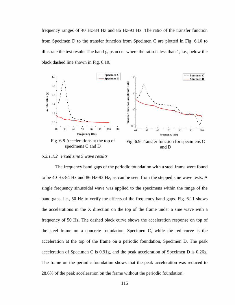
115
frequency ranges of 40 Hz-84 Hz and 86 Hz-93 Hz. The ratio of the transfer function
from Specimen D to the transfer function from Specimen C are plotted in Fig. 6.10 to
illustrate the test results The band gaps occur where the ratio is less than 1, i.e., below the
black dashed line shown in Fig. 6.10.
6.2.1.1.2 Fixed sine S wave results
The frequency band gaps of the periodic foundation with a steel frame were found
to be 40 Hz-84 Hz and 86 Hz-93 Hz, as can be seen from the stepped sine wave tests. A
single frequency sinusoidal wave was applied to the specimens within the range of the
band gaps, i.e., 50 Hz to verify the effects of the frequency band gaps. Fig. 6.11 shows
the accelerations in the X direction on the top of the frame under a sine wave with a
frequency of 50 Hz. The dashed black curve shows the acceleration response on top of
the steel frame on a concrete foundation, Specimen C, while the red curve is the
acceleration at the top of the frame on a periodic foundation, Specimen D. The peak
acceleration of Specimen C is 0.91g, and the peak acceleration of Specimen D is 0.26g.
The frame on the periodic foundation shows that the peak acceleration was reduced to
28.6% of the peak acceleration on the frame without the periodic foundation.
Fig. 6.8 Accelerations at the top of
specimens C and D
Fig. 6.9 Transfer function for specimens C
and D
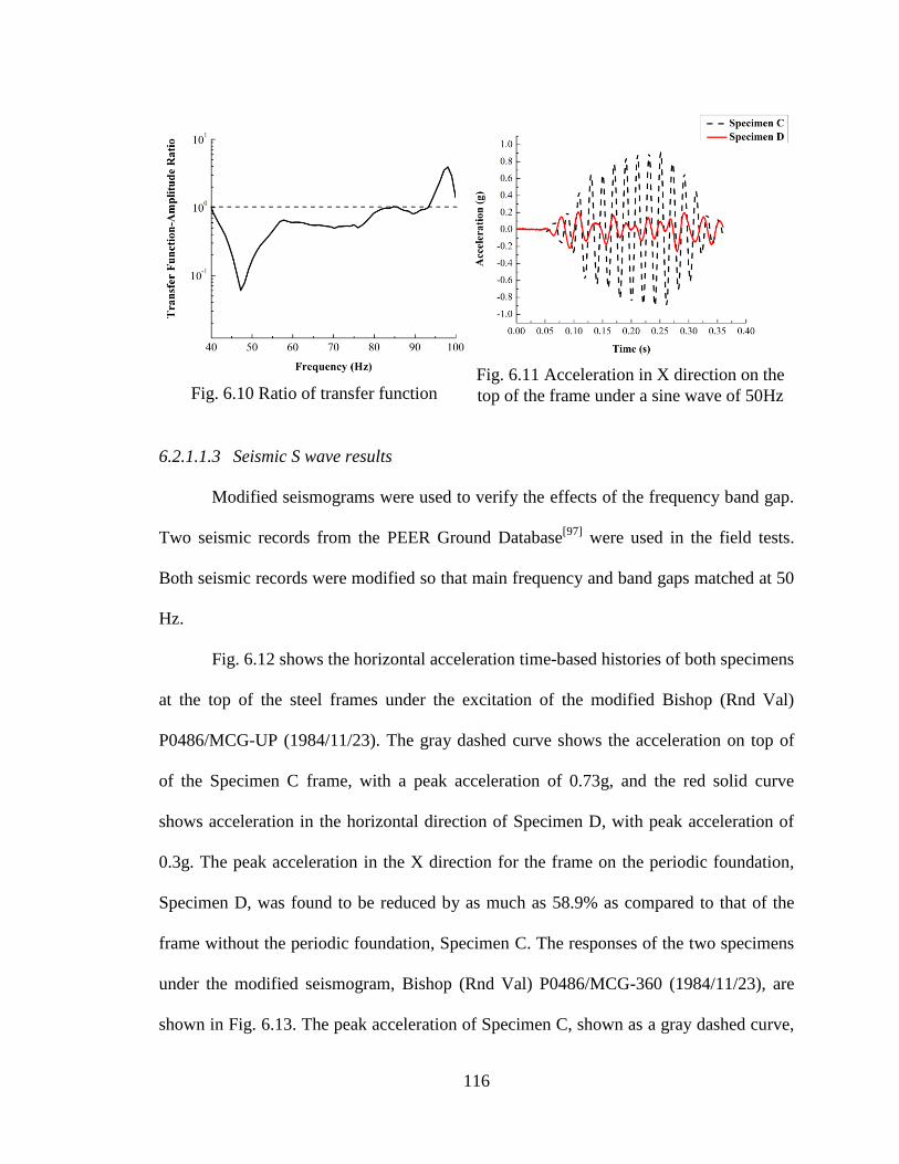
116
6.2.1.1.3 Seismic S wave results
Modified seismograms were used to verify the effects of the frequency band gap.
Two seismic records from the PEER Ground Database[97]
were used in the field tests.
Both seismic records were modified so that main frequency and band gaps matched at 50
Hz.
Fig. 6.12 shows the horizontal acceleration time-based histories of both specimens
at the top of the steel frames under the excitation of the modified Bishop (Rnd Val)
P0486/MCG-UP (1984/11/23). The gray dashed curve shows the acceleration on top of
of the Specimen C frame, with a peak acceleration of 0.73g, and the red solid curve
shows acceleration in the horizontal direction of Specimen D, with peak acceleration of
0.3g. The peak acceleration in the X direction for the frame on the periodic foundation,
Specimen D, was found to be reduced by as much as 58.9% as compared to that of the
frame without the periodic foundation, Specimen C. The responses of the two specimens
under the modified seismogram, Bishop (Rnd Val) P0486/MCG-360 (1984/11/23), are
shown in Fig. 6.13. The peak acceleration of Specimen C, shown as a gray dashed curve,
Fig. 6.10 Ratio of transfer function
Fig. 6.11 Acceleration in X direction on the
top of the frame under a sine wave of 50Hz
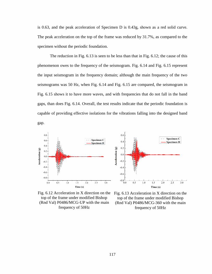
117
is 0.63, and the peak acceleration of Specimen D is 0.43g, shown as a red solid curve.
The peak acceleration on the top of the frame was reduced by 31.7%, as compared to the
specimen without the periodic foundation.
The reduction in Fig. 6.13 is seen to be less than that in Fig. 6.12; the cause of this
phenomenon owes to the frequency of the seismogram. Fig. 6.14 and Fig. 6.15 represent
the input seismogram in the frequency domain; although the main frequency of the two
seismograms was 50 Hz, when Fig. 6.14 and Fig. 6.15 are compared, the seismogram in
Fig. 6.15 shows it to have more waves, and with frequencies that do not fall in the band
gaps, than does Fig. 6.14. Overall, the test results indicate that the periodic foundation is
capable of providing effective isolations for the vibrations falling into the designed band
gap.
Fig. 6.12 Acceleration in X direction on the
top of the frame under modified Bishop
(Rnd Val) P0486/MCG-UP with the main
frequency of 50Hz
Fig. 6.13 Acceleration in X direction on the
top of the frame under modified Bishop
(Rnd Val) P0486/MCG-360 with the main
frequency of 50Hz
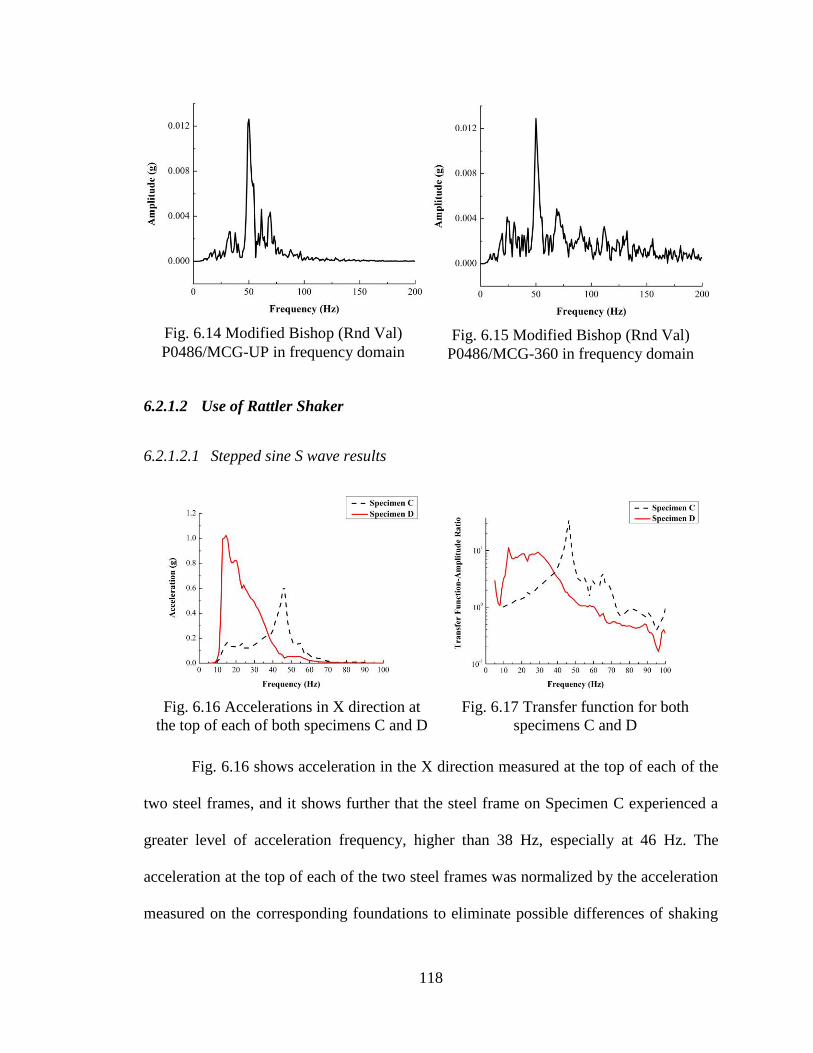
118
6.2.1.2 Use of Rattler Shaker
6.2.1.2.1 Stepped sine S wave results
Fig. 6.16 shows acceleration in the X direction measured at the top of each of the
two steel frames, and it shows further that the steel frame on Specimen C experienced a
greater level of acceleration frequency, higher than 38 Hz, especially at 46 Hz. The
acceleration at the top of each of the two steel frames was normalized by the acceleration
measured on the corresponding foundations to eliminate possible differences of shaking
Fig. 6.14 Modified Bishop (Rnd Val)
P0486/MCG-UP in frequency domain
Fig. 6.15 Modified Bishop (Rnd Val)
P0486/MCG-360 in frequency domain
Fig. 6.16 Accelerations in X direction at
the top of each of both specimens C and D
Fig. 6.17 Transfer function for both
specimens C and D
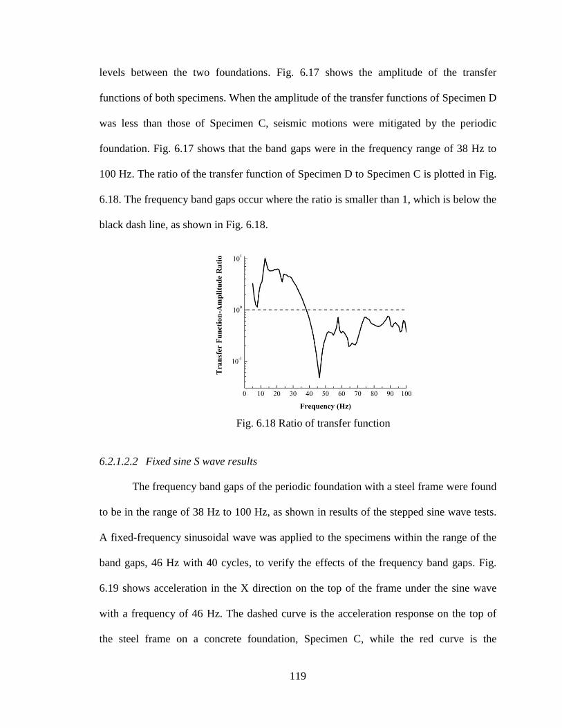
119
levels between the two foundations. Fig. 6.17 shows the amplitude of the transfer
functions of both specimens. When the amplitude of the transfer functions of Specimen D
was less than those of Specimen C, seismic motions were mitigated by the periodic
foundation. Fig. 6.17 shows that the band gaps were in the frequency range of 38 Hz to
100 Hz. The ratio of the transfer function of Specimen D to Specimen C is plotted in Fig.
6.18. The frequency band gaps occur where the ratio is smaller than 1, which is below the
black dash line, as shown in Fig. 6.18.
6.2.1.2.2 Fixed sine S wave results
The frequency band gaps of the periodic foundation with a steel frame were found
to be in the range of 38 Hz to 100 Hz, as shown in results of the stepped sine wave tests.
A fixed-frequency sinusoidal wave was applied to the specimens within the range of the
band gaps, 46 Hz with 40 cycles, to verify the effects of the frequency band gaps. Fig.
6.19 shows acceleration in the X direction on the top of the frame under the sine wave
with a frequency of 46 Hz. The dashed curve is the acceleration response on the top of
the steel frame on a concrete foundation, Specimen C, while the red curve is the
Fig. 6.18 Ratio of transfer function
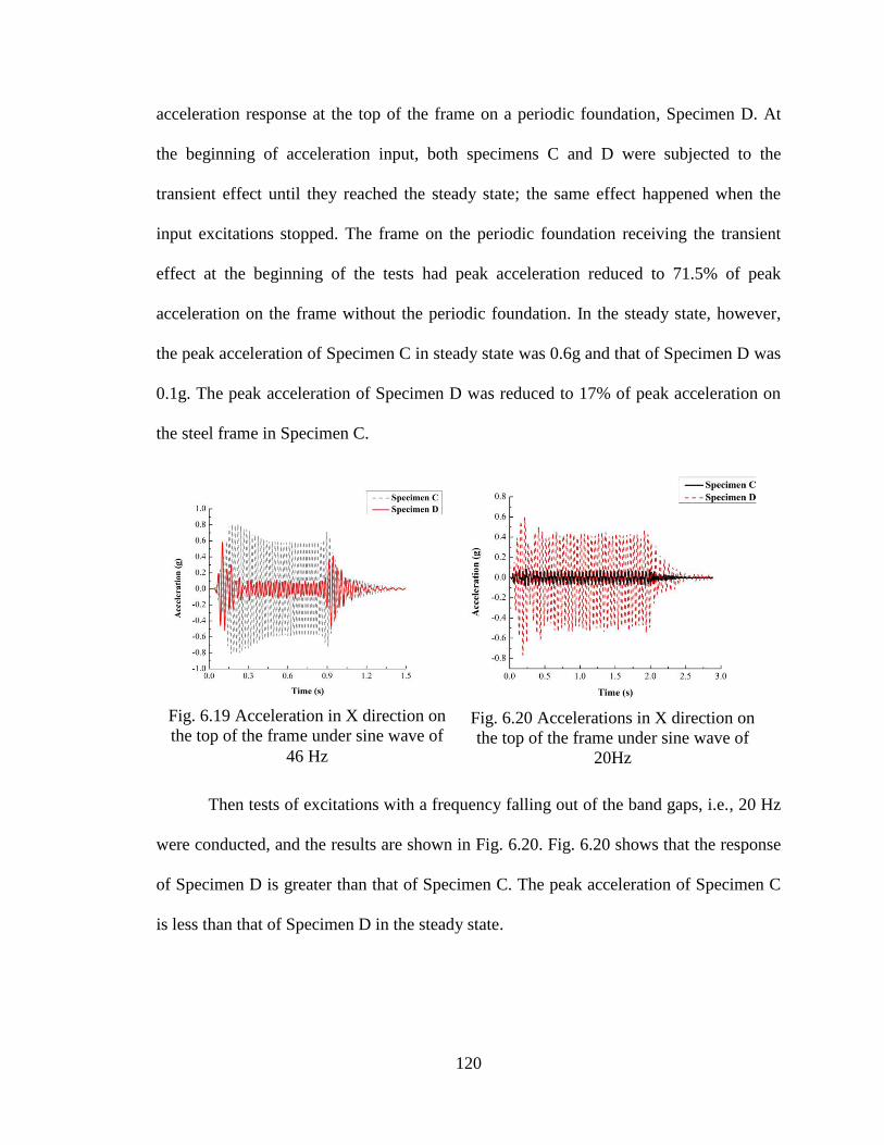
120
acceleration response at the top of the frame on a periodic foundation, Specimen D. At
the beginning of acceleration input, both specimens C and D were subjected to the
transient effect until they reached the steady state; the same effect happened when the
input excitations stopped. The frame on the periodic foundation receiving the transient
effect at the beginning of the tests had peak acceleration reduced to 71.5% of peak
acceleration on the frame without the periodic foundation. In the steady state, however,
the peak acceleration of Specimen C in steady state was 0.6g and that of Specimen D was
0.1g. The peak acceleration of Specimen D was reduced to 17% of peak acceleration on
the steel frame in Specimen C.
Then tests of excitations with a frequency falling out of the band gaps, i.e., 20 Hz
were conducted, and the results are shown in Fig. 6.20. Fig. 6.20 shows that the response
of Specimen D is greater than that of Specimen C. The peak acceleration of Specimen C
is less than that of Specimen D in the steady state.
Fig. 6.19 Acceleration in X direction on
the top of the frame under sine wave of
46 Hz
Fig. 6.20 Accelerations in X direction on
the top of the frame under sine wave of
20Hz
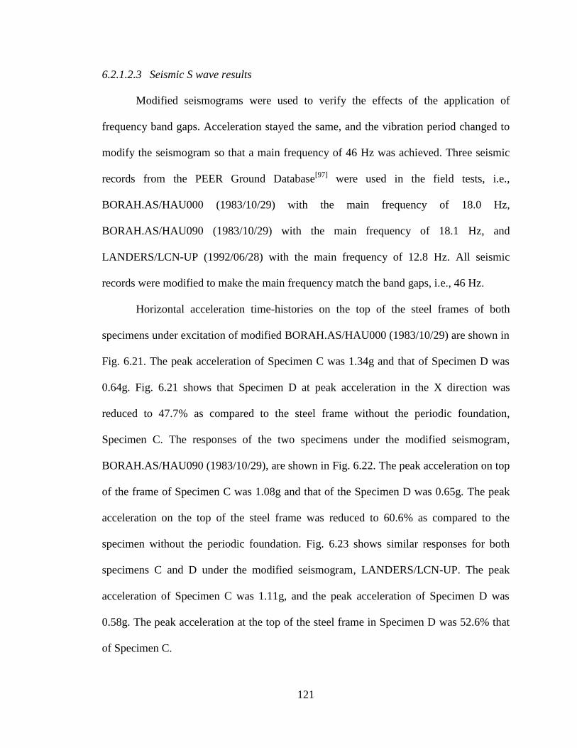
121
6.2.1.2.3 Seismic S wave results
Modified seismograms were used to verify the effects of the application of
frequency band gaps. Acceleration stayed the same, and the vibration period changed to
modify the seismogram so that a main frequency of 46 Hz was achieved. Three seismic
records from the PEER Ground Database[97]
were used in the field tests, i.e.,
BORAH.AS/HAU000 (1983/10/29) with the main frequency of 18.0 Hz,
BORAH.AS/HAU090 (1983/10/29) with the main frequency of 18.1 Hz, and
LANDERS/LCN-UP (1992/06/28) with the main frequency of 12.8 Hz. All seismic
records were modified to make the main frequency match the band gaps, i.e., 46 Hz.
Horizontal acceleration time-histories on the top of the steel frames of both
specimens under excitation of modified BORAH.AS/HAU000 (1983/10/29) are shown in
Fig. 6.21. The peak acceleration of Specimen C was 1.34g and that of Specimen D was
0.64g. Fig. 6.21 shows that Specimen D at peak acceleration in the X direction was
reduced to 47.7% as compared to the steel frame without the periodic foundation,
Specimen C. The responses of the two specimens under the modified seismogram,
BORAH.AS/HAU090 (1983/10/29), are shown in Fig. 6.22. The peak acceleration on top
of the frame of Specimen C was 1.08g and that of the Specimen D was 0.65g. The peak
acceleration on the top of the steel frame was reduced to 60.6% as compared to the
specimen without the periodic foundation. Fig. 6.23 shows similar responses for both
specimens C and D under the modified seismogram, LANDERS/LCN-UP. The peak
acceleration of Specimen C was 1.11g, and the peak acceleration of Specimen D was
0.58g. The peak acceleration at the top of the steel frame in Specimen D was 52.6% that
of Specimen C.
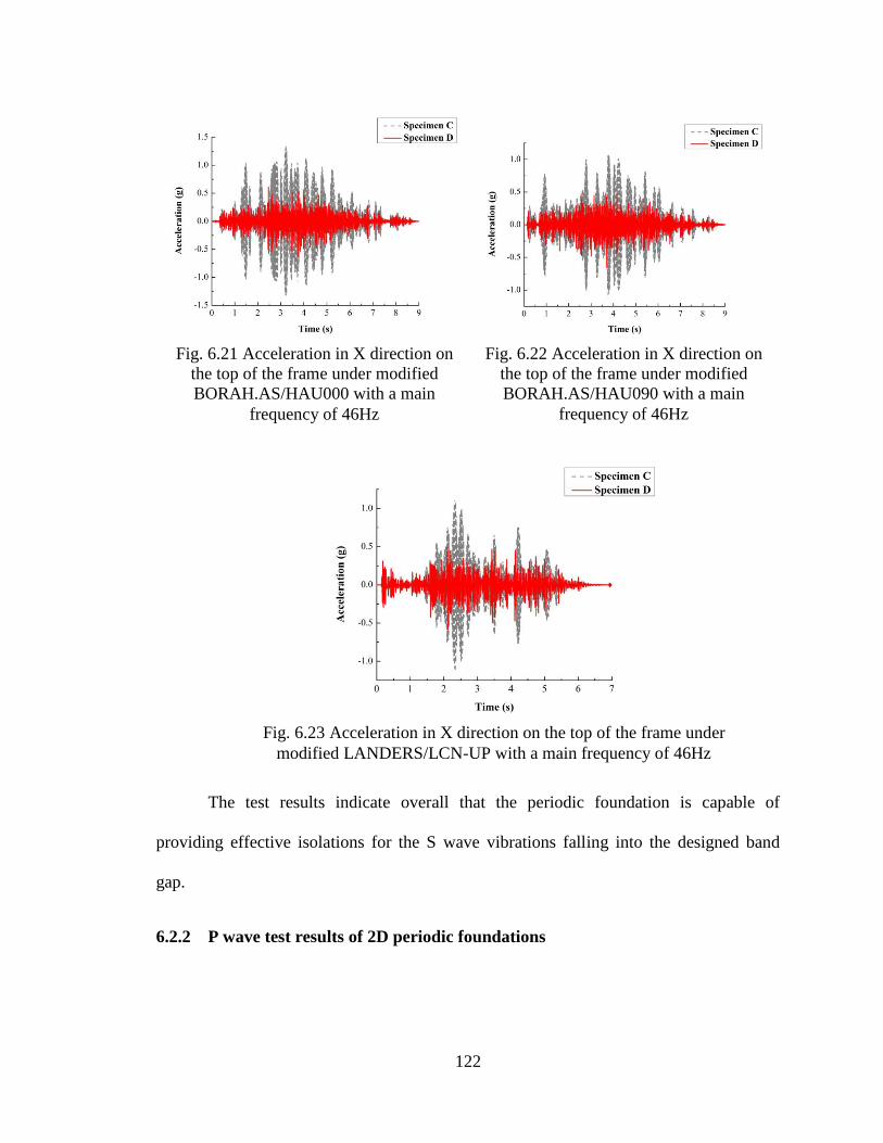
122
The test results indicate overall that the periodic foundation is capable of
providing effective isolations for the S wave vibrations falling into the designed band
gap.
6.2.2 P wave test results of 2D periodic foundations
Fig. 6.21 Acceleration in X direction on
the top of the frame under modified
BORAH.AS/HAU000 with a main
frequency of 46Hz
Fig. 6.22 Acceleration in X direction on
the top of the frame under modified
BORAH.AS/HAU090 with a main
frequency of 46Hz
Fig. 6.23 Acceleration in X direction on the top of the frame under
modified LANDERS/LCN-UP with a main frequency of 46Hz
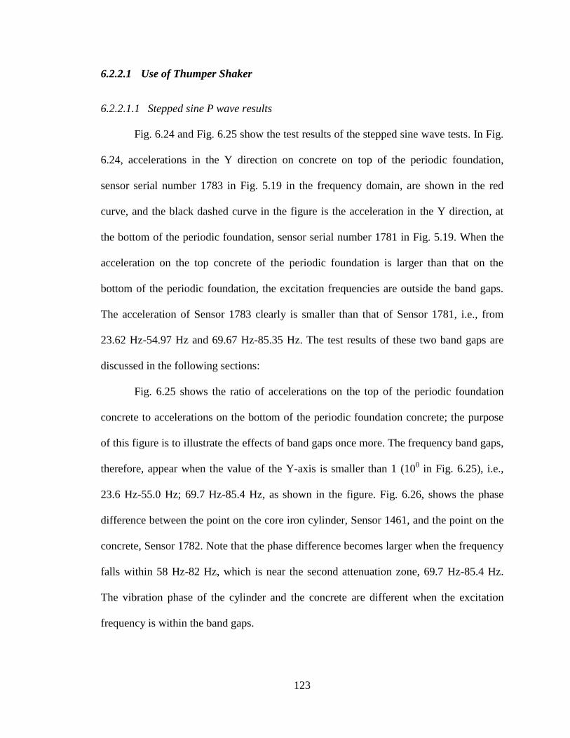
123
6.2.2.1 Use of Thumper Shaker
6.2.2.1.1 Stepped sine P wave results
Fig. 6.24 and Fig. 6.25 show the test results of the stepped sine wave tests. In Fig.
6.24, accelerations in the Y direction on concrete on top of the periodic foundation,
sensor serial number 1783 in Fig. 5.19 in the frequency domain, are shown in the red
curve, and the black dashed curve in the figure is the acceleration in the Y direction, at
the bottom of the periodic foundation, sensor serial number 1781 in Fig. 5.19. When the
acceleration on the top concrete of the periodic foundation is larger than that on the
bottom of the periodic foundation, the excitation frequencies are outside the band gaps.
The acceleration of Sensor 1783 clearly is smaller than that of Sensor 1781, i.e., from
23.62 Hz-54.97 Hz and 69.67 Hz-85.35 Hz. The test results of these two band gaps are
discussed in the following sections:
Fig. 6.25 shows the ratio of accelerations on the top of the periodic foundation
concrete to accelerations on the bottom of the periodic foundation concrete; the purpose
of this figure is to illustrate the effects of band gaps once more. The frequency band gaps,
therefore, appear when the value of the Y-axis is smaller than 1 (100 in Fig. 6.25), i.e.,
23.6 Hz-55.0 Hz; 69.7 Hz-85.4 Hz, as shown in the figure. Fig. 6.26, shows the phase
difference between the point on the core iron cylinder, Sensor 1461, and the point on the
concrete, Sensor 1782. Note that the phase difference becomes larger when the frequency
falls within 58 Hz-82 Hz, which is near the second attenuation zone, 69.7 Hz-85.4 Hz.
The vibration phase of the cylinder and the concrete are different when the excitation
frequency is within the band gaps.
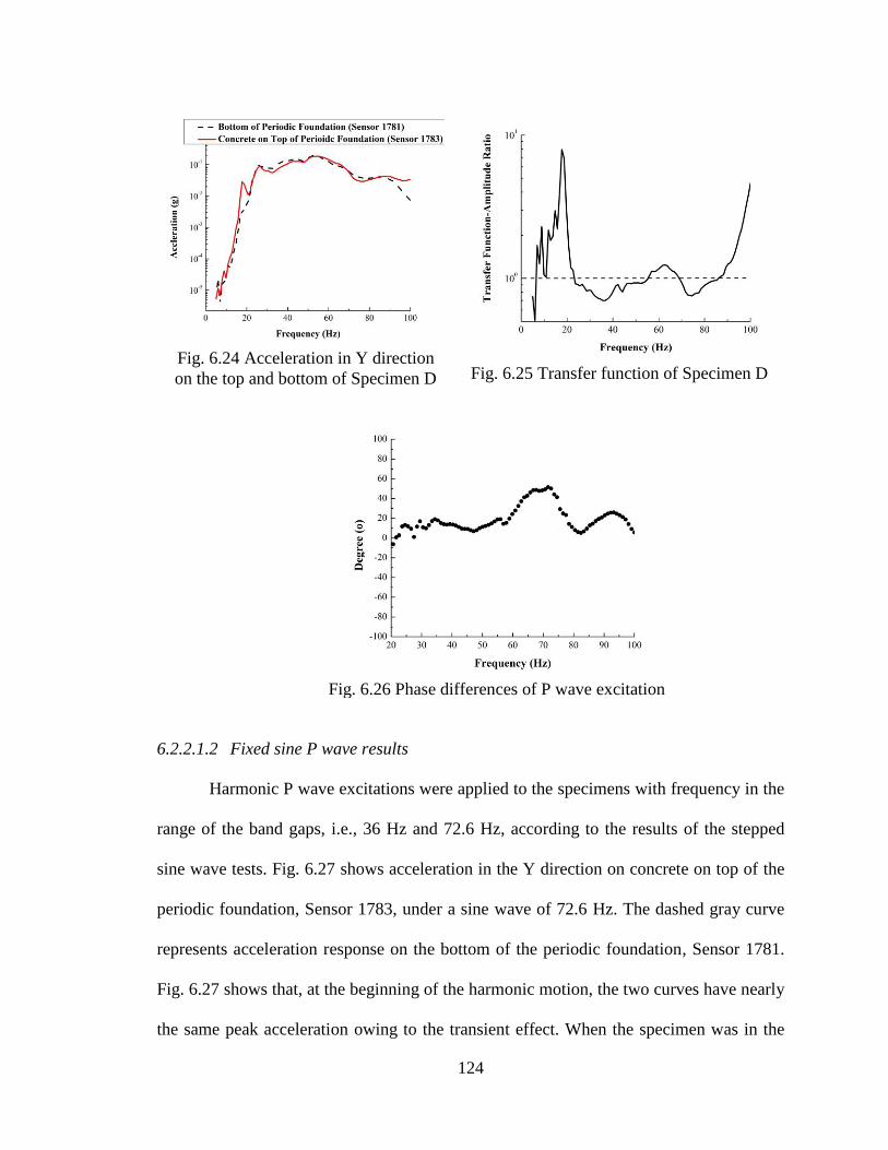
124
6.2.2.1.2 Fixed sine P wave results
Harmonic P wave excitations were applied to the specimens with frequency in the
range of the band gaps, i.e., 36 Hz and 72.6 Hz, according to the results of the stepped
sine wave tests. Fig. 6.27 shows acceleration in the Y direction on concrete on top of the
periodic foundation, Sensor 1783, under a sine wave of 72.6 Hz. The dashed gray curve
represents acceleration response on the bottom of the periodic foundation, Sensor 1781.
Fig. 6.27 shows that, at the beginning of the harmonic motion, the two curves have nearly
the same peak acceleration owing to the transient effect. When the specimen was in the
Fig. 6.24 Acceleration in Y direction
on the top and bottom of Specimen D
Fig. 6.25 Transfer function of Specimen D
Fig. 6.26 Phase differences of P wave excitation
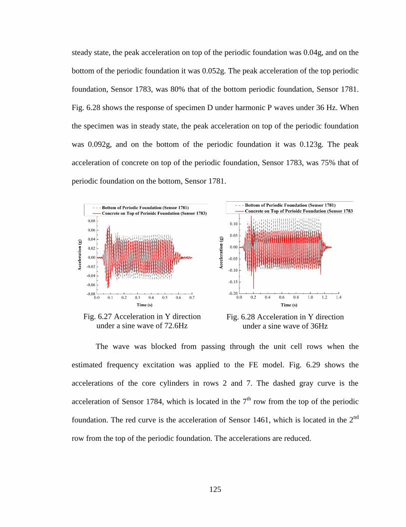
125
steady state, the peak acceleration on top of the periodic foundation was 0.04g, and on the
bottom of the periodic foundation it was 0.052g. The peak acceleration of the top periodic
foundation, Sensor 1783, was 80% that of the bottom periodic foundation, Sensor 1781.
Fig. 6.28 shows the response of specimen D under harmonic P waves under 36 Hz. When
the specimen was in steady state, the peak acceleration on top of the periodic foundation
was 0.092g, and on the bottom of the periodic foundation it was 0.123g. The peak
acceleration of concrete on top of the periodic foundation, Sensor 1783, was 75% that of
periodic foundation on the bottom, Sensor 1781.
The wave was blocked from passing through the unit cell rows when the
estimated frequency excitation was applied to the FE model. Fig. 6.29 shows the
accelerations of the core cylinders in rows 2 and 7. The dashed gray curve is the
acceleration of Sensor 1784, which is located in the 7th
row from the top of the periodic
foundation. The red curve is the acceleration of Sensor 1461, which is located in the 2nd
row from the top of the periodic foundation. The accelerations are reduced.
Fig. 6.27 Acceleration in Y direction
under a sine wave of 72.6Hz
Fig. 6.28 Acceleration in Y direction
under a sine wave of 36Hz
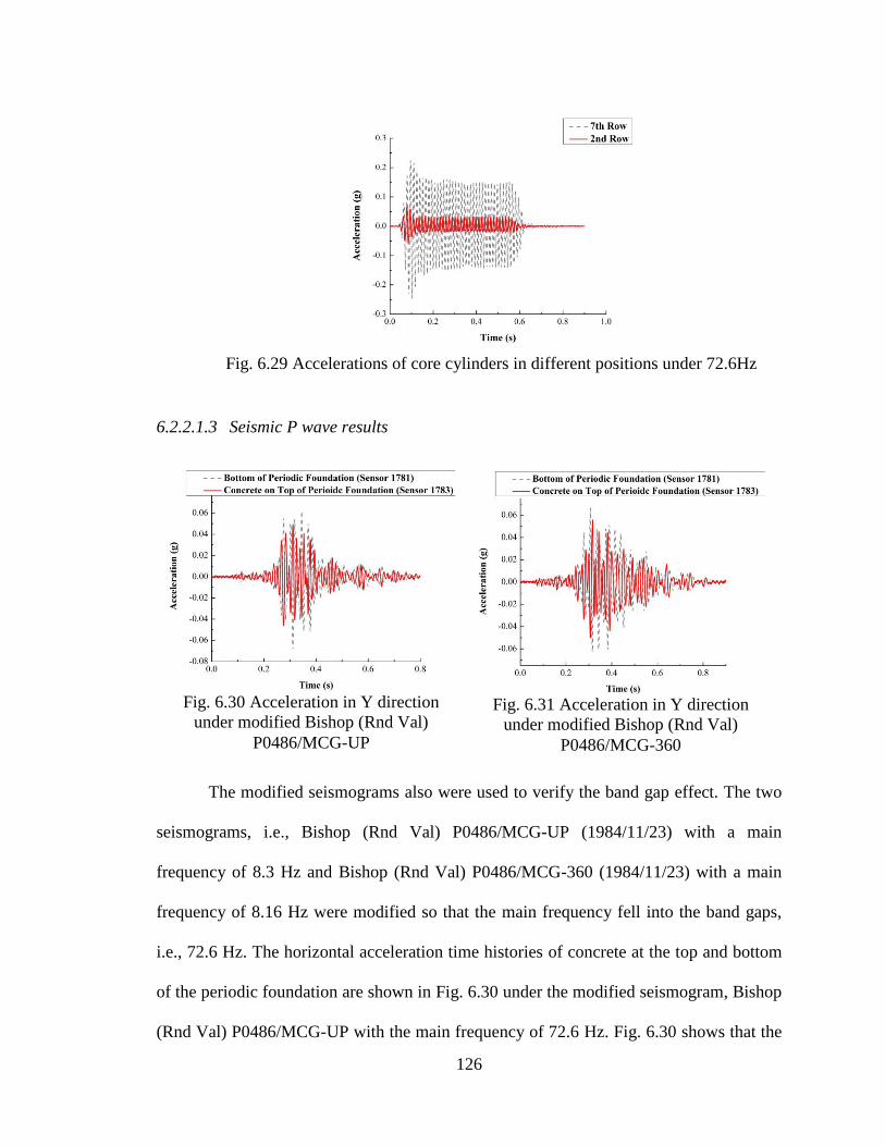
126
6.2.2.1.3 Seismic P wave results
The modified seismograms also were used to verify the band gap effect. The two
seismograms, i.e., Bishop (Rnd Val) P0486/MCG-UP (1984/11/23) with a main
frequency of 8.3 Hz and Bishop (Rnd Val) P0486/MCG-360 (1984/11/23) with a main
frequency of 8.16 Hz were modified so that the main frequency fell into the band gaps,
i.e., 72.6 Hz. The horizontal acceleration time histories of concrete at the top and bottom
of the periodic foundation are shown in Fig. 6.30 under the modified seismogram, Bishop
(Rnd Val) P0486/MCG-UP with the main frequency of 72.6 Hz. Fig. 6.30 shows that the
Fig. 6.29 Accelerations of core cylinders in different positions under 72.6Hz
Fig. 6.30 Acceleration in Y direction
under modified Bishop (Rnd Val)
P0486/MCG-UP
Fig. 6.31 Acceleration in Y direction
under modified Bishop (Rnd Val)
P0486/MCG-360
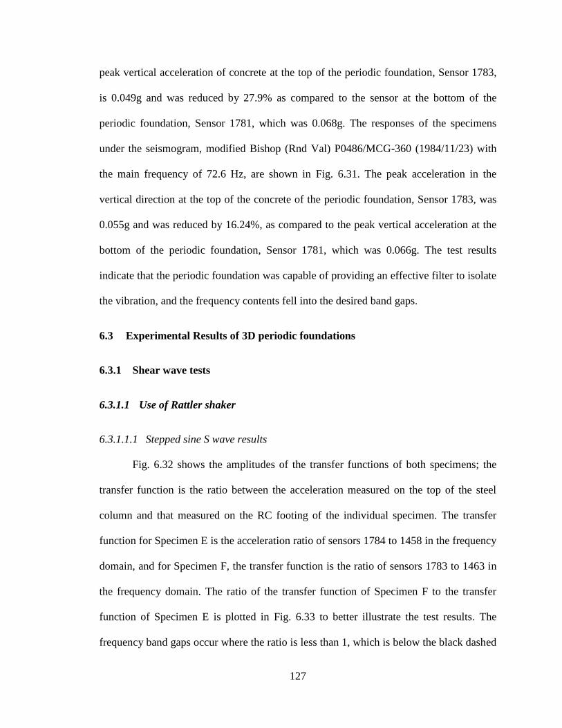
127
peak vertical acceleration of concrete at the top of the periodic foundation, Sensor 1783,
is 0.049g and was reduced by 27.9% as compared to the sensor at the bottom of the
periodic foundation, Sensor 1781, which was 0.068g. The responses of the specimens
under the seismogram, modified Bishop (Rnd Val) P0486/MCG-360 (1984/11/23) with
the main frequency of 72.6 Hz, are shown in Fig. 6.31. The peak acceleration in the
vertical direction at the top of the concrete of the periodic foundation, Sensor 1783, was
0.055g and was reduced by 16.24%, as compared to the peak vertical acceleration at the
bottom of the periodic foundation, Sensor 1781, which was 0.066g. The test results
indicate that the periodic foundation was capable of providing an effective filter to isolate
the vibration, and the frequency contents fell into the desired band gaps.
6.3 Experimental Results of 3D periodic foundations
6.3.1 Shear wave tests
6.3.1.1 Use of Rattler shaker
6.3.1.1.1 Stepped sine S wave results
Fig. 6.32 shows the amplitudes of the transfer functions of both specimens; the
transfer function is the ratio between the acceleration measured on the top of the steel
column and that measured on the RC footing of the individual specimen. The transfer
function for Specimen E is the acceleration ratio of sensors 1784 to 1458 in the frequency
domain, and for Specimen F, the transfer function is the ratio of sensors 1783 to 1463 in
the frequency domain. The ratio of the transfer function of Specimen F to the transfer
function of Specimen E is plotted in Fig. 6.33 to better illustrate the test results. The
frequency band gaps occur where the ratio is less than 1, which is below the black dashed
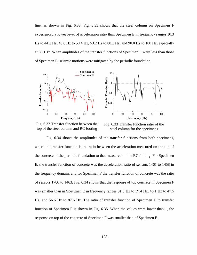
128
line, as shown in Fig. 6.33. Fig. 6.33 shows that the steel column on Specimen F
experienced a lower level of acceleration ratio than Specimen E in frequency ranges 10.3
Hz to 44.1 Hz, 45.6 Hz to 50.4 Hz, 53.2 Hz to 88.1 Hz, and 90.0 Hz to 100 Hz, especially
at 35.1Hz. When amplitudes of the transfer functions of Specimen F were less than those
of Specimen E, seismic motions were mitigated by the periodic foundation.
Fig. 6.34 shows the amplitudes of the transfer functions from both specimens,
where the transfer function is the ratio between the acceleration measured on the top of
the concrete of the periodic foundation to that measured on the RC footing. For Specimen
E, the transfer function of concrete was the acceleration ratio of sensors 1461 to 1458 in
the frequency domain, and for Specimen F the transfer function of concrete was the ratio
of sensors 1780 to 1463. Fig. 6.34 shows that the response of top concrete in Specimen F
was smaller than in Specimen E in frequency ranges 31.3 Hz to 39.4 Hz, 46.1 Hz to 47.5
Hz, and 56.6 Hz to 87.6 Hz. The ratio of transfer function of Specimen E to transfer
function of Specimen F is shown in Fig. 6.35. When the values were lower than 1, the
response on top of the concrete of Specimen F was smaller than of Specimen E.
Fig. 6.32 Transfer function between the
top of the steel column and RC footing
Fig. 6.33 Transfer function ratio of the
steel column for the specimens
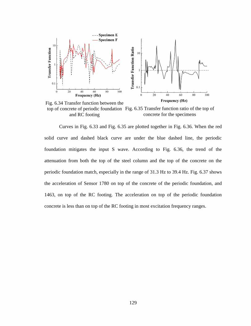
129
Curves in Fig. 6.33 and Fig. 6.35 are plotted together in Fig. 6.36. When the red
solid curve and dashed black curve are under the blue dashed line, the periodic
foundation mitigates the input S wave. According to Fig. 6.36, the trend of the
attenuation from both the top of the steel column and the top of the concrete on the
periodic foundation match, especially in the range of 31.3 Hz to 39.4 Hz. Fig. 6.37 shows
the acceleration of Sensor 1780 on top of the concrete of the periodic foundation, and
1463, on top of the RC footing. The acceleration on top of the periodic foundation
concrete is less than on top of the RC footing in most excitation frequency ranges.
Fig. 6.34 Transfer function between the
top of concrete of periodic foundation
and RC footing
Fig. 6.35 Transfer function ratio of the top of
concrete for the specimens
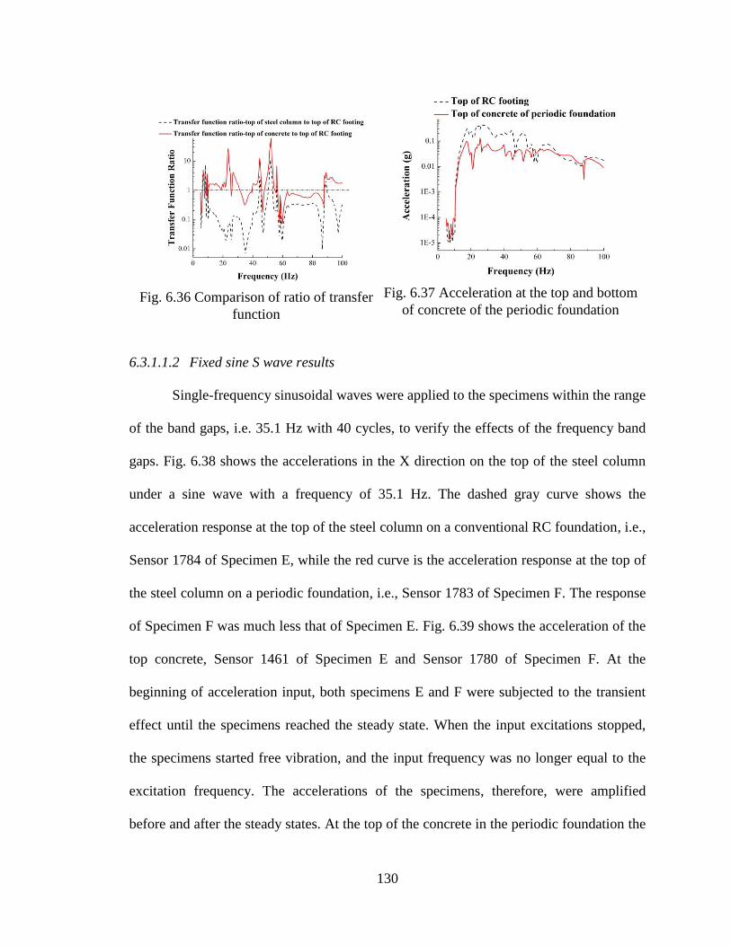
130
6.3.1.1.2 Fixed sine S wave results
Single-frequency sinusoidal waves were applied to the specimens within the range
of the band gaps, i.e. 35.1 Hz with 40 cycles, to verify the effects of the frequency band
gaps. Fig. 6.38 shows the accelerations in the X direction on the top of the steel column
under a sine wave with a frequency of 35.1 Hz. The dashed gray curve shows the
acceleration response at the top of the steel column on a conventional RC foundation, i.e.,
Sensor 1784 of Specimen E, while the red curve is the acceleration response at the top of
the steel column on a periodic foundation, i.e., Sensor 1783 of Specimen F. The response
of Specimen F was much less that of Specimen E. Fig. 6.39 shows the acceleration of the
top concrete, Sensor 1461 of Specimen E and Sensor 1780 of Specimen F. At the
beginning of acceleration input, both specimens E and F were subjected to the transient
effect until the specimens reached the steady state. When the input excitations stopped,
the specimens started free vibration, and the input frequency was no longer equal to the
excitation frequency. The accelerations of the specimens, therefore, were amplified
before and after the steady states. At the top of the concrete in the periodic foundation the
Fig. 6.36 Comparison of ratio of transfer
function
Fig. 6.37 Acceleration at the top and bottom
of concrete of the periodic foundation
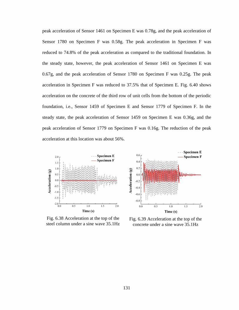
131
peak acceleration of Sensor 1461 on Specimen E was 0.78g, and the peak acceleration of
Sensor 1780 on Specimen F was 0.58g. The peak acceleration in Specimen F was
reduced to 74.8% of the peak acceleration as compared to the traditional foundation. In
the steady state, however, the peak acceleration of Sensor 1461 on Specimen E was
0.67g, and the peak acceleration of Sensor 1780 on Specimen F was 0.25g. The peak
acceleration in Specimen F was reduced to 37.5% that of Specimen E. Fig. 6.40 shows
acceleration on the concrete of the third row of unit cells from the bottom of the periodic
foundation, i.e., Sensor 1459 of Specimen E and Sensor 1779 of Specimen F. In the
steady state, the peak acceleration of Sensor 1459 on Specimen E was 0.36g, and the
peak acceleration of Sensor 1779 on Specimen F was 0.16g. The reduction of the peak
acceleration at this location was about 56%.
Fig. 6.38 Acceleration at the top of the
steel column under a sine wave 35.1Hz
Fig. 6.39 Acceleration at the top of the
concrete under a sine wave 35.1Hz
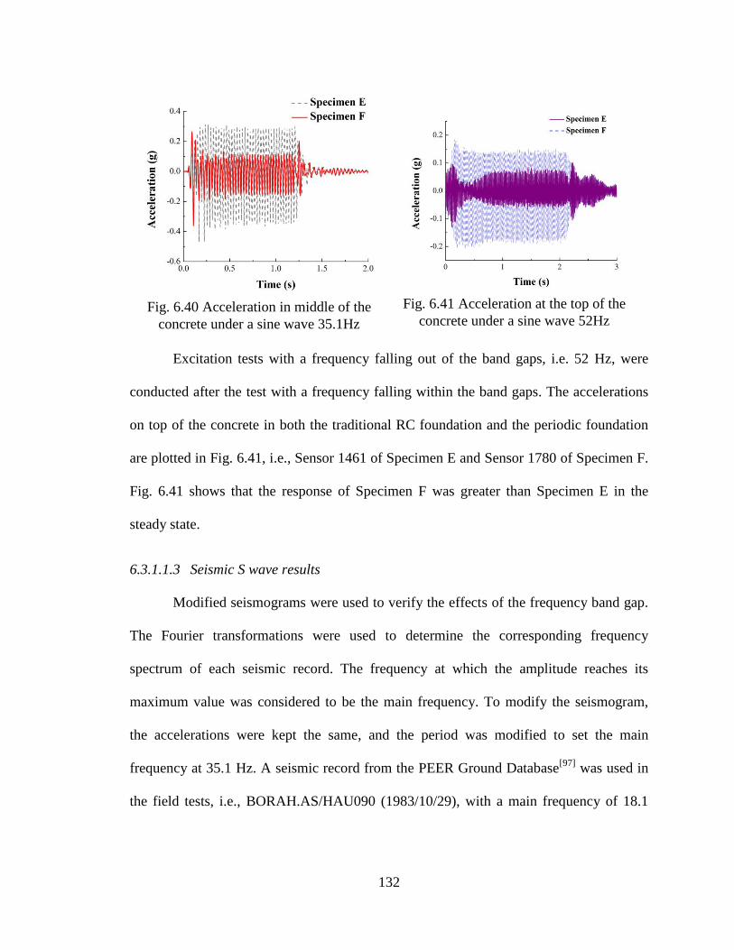
132
Excitation tests with a frequency falling out of the band gaps, i.e. 52 Hz, were
conducted after the test with a frequency falling within the band gaps. The accelerations
on top of the concrete in both the traditional RC foundation and the periodic foundation
are plotted in Fig. 6.41, i.e., Sensor 1461 of Specimen E and Sensor 1780 of Specimen F.
Fig. 6.41 shows that the response of Specimen F was greater than Specimen E in the
steady state.
6.3.1.1.3 Seismic S wave results
Modified seismograms were used to verify the effects of the frequency band gap.
The Fourier transformations were used to determine the corresponding frequency
spectrum of each seismic record. The frequency at which the amplitude reaches its
maximum value was considered to be the main frequency. To modify the seismogram,
the accelerations were kept the same, and the period was modified to set the main
frequency at 35.1 Hz. A seismic record from the PEER Ground Database[97]
was used in
the field tests, i.e., BORAH.AS/HAU090 (1983/10/29), with a main frequency of 18.1
Fig. 6.40 Acceleration in middle of the
concrete under a sine wave 35.1Hz
Fig. 6.41 Acceleration at the top of the
concrete under a sine wave 52Hz
133
Hz. The seismic record was modified so that the main frequency matched the band gap
frequency, i.e., 35.1 Hz.
The acceleration in the X direction of each sensor was recorded in the time
domain. Fig. 6.42 shows the horizontal acceleration time-histories on the top of the steel
column from both specimens under the excitations of the modified BORAH.AS/HAU090
(1983/10/29), Fig. 6.42 shows that, for the steel column on the periodic foundation, i.e.,
with a peak acceleration of 0.14g from Sensor 1783, the peak acceleration in the X
direction was reduced to 8.08% as compared to that of the steel column with the
conventional foundation, i.e., with a peak acceleration of 1.73g from Sensor 1784. The
responses at the top of the concrete of the two specimens, i.e., sensors 1461 and 1780, are
shown in Fig. 6.43. The peak acceleration on the top of the concrete of Specimen F, with
a peak acceleration of 0.55g from Sensor 1780, was reduced to 76.76%, as compared to
Specimen E, with a peak acceleration of 0.72g from Sensor 1461, with the conventional
foundation. Fig. 6.44 shows similar responses for the two specimens, E and F. The red
curve is the acceleration of the concrete in the middle of the periodic foundation, with a
peak acceleration of 0.34g from Sensor 1779, and the gray curve is the acceleration of the
concrete in the middle of the conventional foundation, with a peak acceleration of 0.45g
from Sensor 1459. The peak acceleration at the top of the concrete in Specimen F was
75.2% that of Specimen E.
Overall, the test results indicate that the periodic foundation is capable of
providing effective isolation for the S wave vibrations falling into the designed band gap.

134
6.3.1.2 Use of T-Rex shaker
6.3.1.2.1 Stepped sine S wave results
Fig. 6.45 shows the transfer functions of Specimen F under 2V and 4.5V
excitations, where the transfer function is the ratio of the acceleration measured on the
top of the steel column relative to the acceleration measured on the RC footing of the
Fig. 6.42 Acceleration in X direction at
the top of the column under modified
BORAH.AS/HAU090 with a main
frequency of 35.1Hz
Fig. 6.43 Acceleration in X direction at
the top of concrete under modified
BORAH.AS/HAU090 with a main
frequency of 35.1Hz
Fig. 6.44 Acceleration in X direction in the middle of the
concrete under modified BORAH.AS/HAU090 with a
main frequency of 35.1Hz
135
individual specimen. The transfer function of Specimen F is the ratio of sensors 1783 to
1463 in the frequency domain. The transfer function of Specimen E is the acceleration
ratio of sensors 1784 to 1458 in the frequency domain. The attenuation zones of Fig. 6.45
occur where the ratio is smaller than 1. The output value of Specimen F was smaller than
the input when the acceleration on top of the column was smaller than on top of the RC
footing. The attenuation zones under 2V excitation are 40.8 Hz-46.5 Hz and 56 Hz-100
Hz, and the attenuation zones under 4.5V excitation are 37.5 Hz-46.6 Hz and 59.4 Hz-
100 Hz. The results from the gray dashed curve and the red solid curve were in
agreement.
To better illustrate the test results, the ratio of the transfer function of Specimen F
to the transfer function of Specimen E (transfer function amplitude ratio) is plotted in Fig.
6.46. When the values are lower than 1, the transfer function of Specimen F is smaller
than that of Specimen E. Fig. 6.46 shows that, with 4.5V excitation, the steel column on
Specimen F experienced a lower level of accelerations ratio than Specimen E in
frequency ranges 5 Hz-48.4 Hz, 53.7 Hz-58 Hz, and 59.4 Hz-88.1 Hz, especially at 43.7
Hz. Fig. 6.47 shows the transfer function amplitude ratio on the concrete of the two
specimens. The transfer function on top of the concrete for Specimen E is the ratio of
sensors 1461 to 1458, and the transfer function on top of the concrete for Specimen F is
the ratio of sensors 1780 to 1463. The transfer function amplitude ratio in Fig. 6.47 is the
ratio of the transfer function on top of the concrete of Specimen F to that of Specimen E.
Fig. 6.47 shows that with 4.5V excitation, the concrete on top of Specimen F experienced
a lower level of acceleration ratio than Specimen E in frequency ranges 36.5 Hz-46.5 Hz,
54.4 Hz-57.9 Hz, and 59.9 Hz-89 Hz, especially at 43.7 Hz.
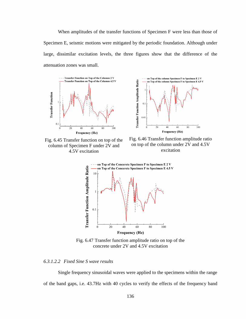
136
When amplitudes of the transfer functions of Specimen F were less than those of
Specimen E, seismic motions were mitigated by the periodic foundation. Although under
large, dissimilar excitation levels, the three figures show that the difference of the
attenuation zones was small.
6.3.1.2.2 Fixed Sine S wave results
Single frequency sinusoidal waves were applied to the specimens within the range
of the band gaps, i.e. 43.7Hz with 40 cycles to verify the effects of the frequency band
Fig. 6.45 Transfer function on top of the
column of Specimen F under 2V and
4.5V excitation
Fig. 6.46 Transfer function amplitude ratio
on top of the column under 2V and 4.5V
excitation
Fig. 6.47 Transfer function amplitude ratio on top of the
concrete under 2V and 4.5V excitation
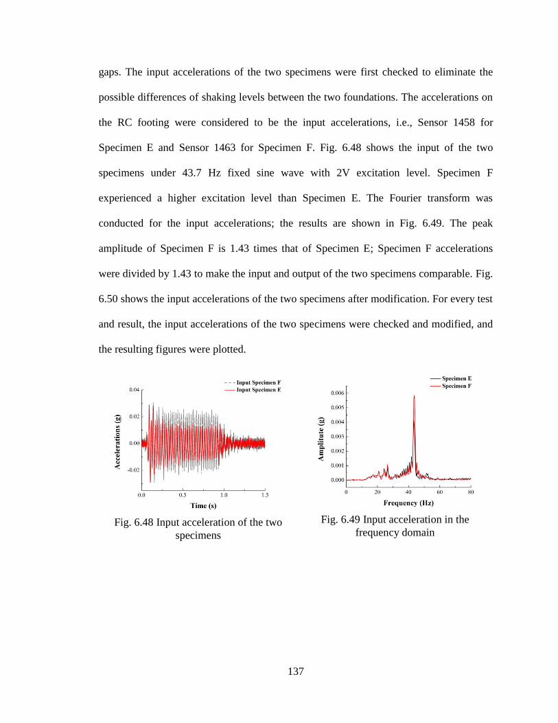
137
gaps. The input accelerations of the two specimens were first checked to eliminate the
possible differences of shaking levels between the two foundations. The accelerations on
the RC footing were considered to be the input accelerations, i.e., Sensor 1458 for
Specimen E and Sensor 1463 for Specimen F. Fig. 6.48 shows the input of the two
specimens under 43.7 Hz fixed sine wave with 2V excitation level. Specimen F
experienced a higher excitation level than Specimen E. The Fourier transform was
conducted for the input accelerations; the results are shown in Fig. 6.49. The peak
amplitude of Specimen F is 1.43 times that of Specimen E; Specimen F accelerations
were divided by 1.43 to make the input and output of the two specimens comparable. Fig.
6.50 shows the input accelerations of the two specimens after modification. For every test
and result, the input accelerations of the two specimens were checked and modified, and
the resulting figures were plotted.
Fig. 6.48 Input acceleration of the two
specimens
Fig. 6.49 Input acceleration in the
frequency domain
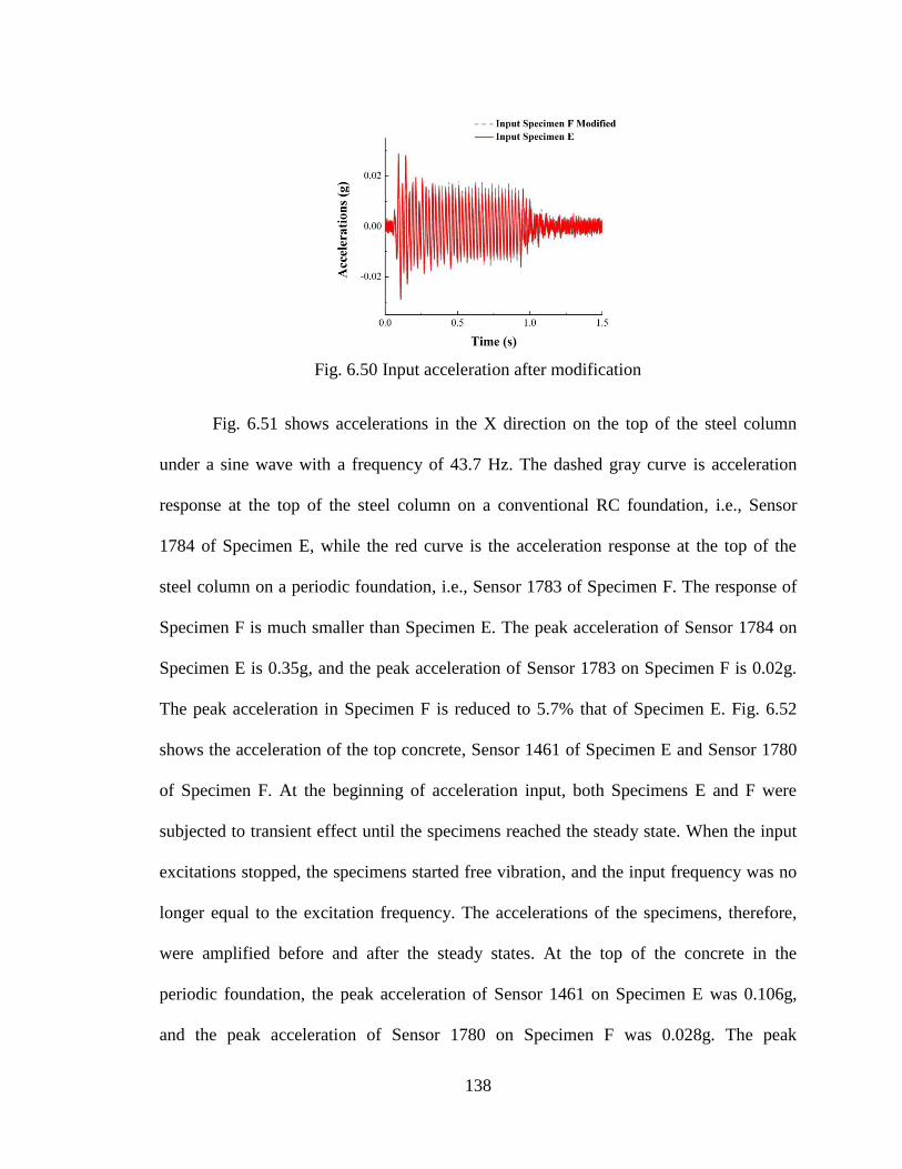
138
Fig. 6.51 shows accelerations in the X direction on the top of the steel column
under a sine wave with a frequency of 43.7 Hz. The dashed gray curve is acceleration
response at the top of the steel column on a conventional RC foundation, i.e., Sensor
1784 of Specimen E, while the red curve is the acceleration response at the top of the
steel column on a periodic foundation, i.e., Sensor 1783 of Specimen F. The response of
Specimen F is much smaller than Specimen E. The peak acceleration of Sensor 1784 on
Specimen E is 0.35g, and the peak acceleration of Sensor 1783 on Specimen F is 0.02g.
The peak acceleration in Specimen F is reduced to 5.7% that of Specimen E. Fig. 6.52
shows the acceleration of the top concrete, Sensor 1461 of Specimen E and Sensor 1780
of Specimen F. At the beginning of acceleration input, both Specimens E and F were
subjected to transient effect until the specimens reached the steady state. When the input
excitations stopped, the specimens started free vibration, and the input frequency was no
longer equal to the excitation frequency. The accelerations of the specimens, therefore,
were amplified before and after the steady states. At the top of the concrete in the
periodic foundation, the peak acceleration of Sensor 1461 on Specimen E was 0.106g,
and the peak acceleration of Sensor 1780 on Specimen F was 0.028g. The peak
Fig. 6.50 Input acceleration after modification

139
acceleration in Specimen F was reduced to 26.4% that of Specimen E. Fig. 6.53 shows
acceleration on the concrete of the third row of unit cells from the bottom of the periodic
foundation, i.e., Sensor 1459 of Specimen E and Sensor 1779 of Specimen F. The peak
acceleration of Sensor 1459 on Specimen E was 0.075g in the steady state, and the peak
acceleration of Sensor 1779 on Specimen F was 0.0185g. The reduction of the peak
acceleration at this location, therefore, was about 75.3%. Fig. 6.54 shows the acceleration
on top of the column and the input acceleration of Specimen F under a 2V fixed sine S
wave of 43.7 Hz. In the steady state, the peak response on top of the column was
0.0113g, which was 43.5% of the peak input acceleration, 0.026g.
Fig. 6.51 Acceleration on top of the
column under 2V fixed sine S wave 43.7
Hz
Fig. 6.52 Acceleration on top of the
concrete under 2V fixed sine S wave 43.7
Hz
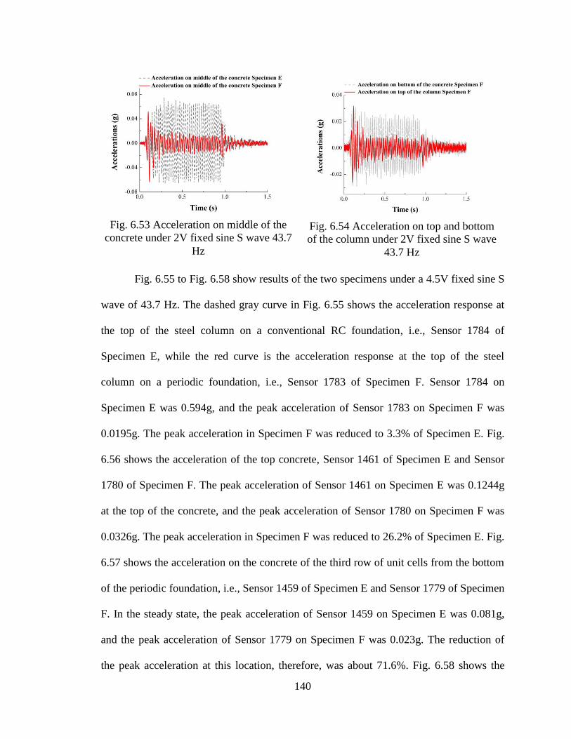
140
Fig. 6.55 to Fig. 6.58 show results of the two specimens under a 4.5V fixed sine S
wave of 43.7 Hz. The dashed gray curve in Fig. 6.55 shows the acceleration response at
the top of the steel column on a conventional RC foundation, i.e., Sensor 1784 of
Specimen E, while the red curve is the acceleration response at the top of the steel
column on a periodic foundation, i.e., Sensor 1783 of Specimen F. Sensor 1784 on
Specimen E was 0.594g, and the peak acceleration of Sensor 1783 on Specimen F was
0.0195g. The peak acceleration in Specimen F was reduced to 3.3% of Specimen E. Fig.
6.56 shows the acceleration of the top concrete, Sensor 1461 of Specimen E and Sensor
1780 of Specimen F. The peak acceleration of Sensor 1461 on Specimen E was 0.1244g
at the top of the concrete, and the peak acceleration of Sensor 1780 on Specimen F was
0.0326g. The peak acceleration in Specimen F was reduced to 26.2% of Specimen E. Fig.
6.57 shows the acceleration on the concrete of the third row of unit cells from the bottom
of the periodic foundation, i.e., Sensor 1459 of Specimen E and Sensor 1779 of Specimen
F. In the steady state, the peak acceleration of Sensor 1459 on Specimen E was 0.081g,
and the peak acceleration of Sensor 1779 on Specimen F was 0.023g. The reduction of
the peak acceleration at this location, therefore, was about 71.6%. Fig. 6.58 shows the
Fig. 6.53 Acceleration on middle of the
concrete under 2V fixed sine S wave 43.7
Hz
Fig. 6.54 Acceleration on top and bottom
of the column under 2V fixed sine S wave
43.7 Hz
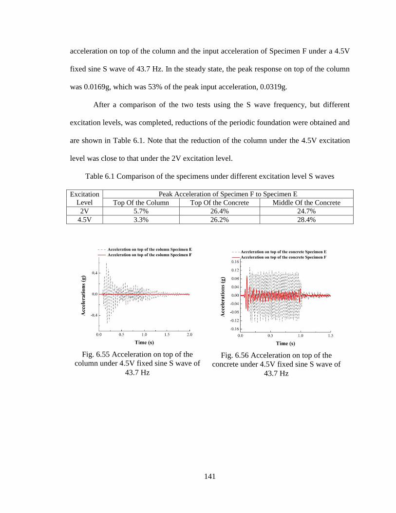
141
acceleration on top of the column and the input acceleration of Specimen F under a 4.5V
fixed sine S wave of 43.7 Hz. In the steady state, the peak response on top of the column
was 0.0169g, which was 53% of the peak input acceleration, 0.0319g.
After a comparison of the two tests using the S wave frequency, but different
excitation levels, was completed, reductions of the periodic foundation were obtained and
are shown in Table 6.1. Note that the reduction of the column under the 4.5V excitation
level was close to that under the 2V excitation level.
Table 6.1 Comparison of the specimens under different excitation level S waves
Excitation
Level
Peak Acceleration of Specimen F to Specimen E
Top Of the Column Top Of the Concrete Middle Of the Concrete
2V 5.7% 26.4% 24.7%
4.5V 3.3% 26.2% 28.4%
Fig. 6.55 Acceleration on top of the
column under 4.5V fixed sine S wave of
43.7 Hz
Fig. 6.56 Acceleration on top of the
concrete under 4.5V fixed sine S wave of
43.7 Hz

142
6.3.1.2.3 Seismic S wave results
Modified seismograms were used to verify the effects of the frequency band gap.
To find the main frequency of each seismic record, the Fourier transformations were used
to determine the corresponding frequency spectrum. The frequency at which the
amplitude reaches its maximum value was considered the main frequency. Acceleration
was kept the same to modify the seismogram, and the period was revised to obtain the
main frequency of 43.7 Hz. A seismic record from the PEER Ground Database[97]
was
used in the field tests, i.e., BORAH.AS/HAU000 (1983/10/29) with a main frequency of
17.3 Hz. The seismic record was modified to make the main frequency match the band
gap frequency, i.e., 43.7 Hz, the same frequency as for the S wave fixed sine tests. There
were two excitation levels for the seismic S wave tests, i.e., 2V and 4.5V.
The acceleration in the X direction of each sensor was recorded in the time
domain. The horizontal acceleration time-histories on the top of the steel column of both
specimens under 2V excitation of the modified BORAH.AS/HAU000 (1983/10/29) are
shown in Fig. 6.59. Fig. 6.59 shows that, for the steel column on the periodic foundation,
Fig. 6.57 Acceleration on middle of the
concrete under 4.5V fixed sine S wave of
43.7 Hz
Fig. 6.58 Acceleration on top of the
concrete under 4.5V fixed sine S wave
of 43.7 Hz
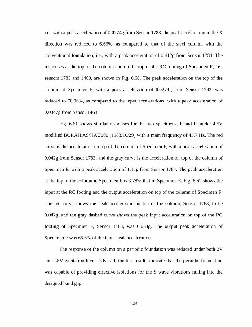
143
i.e., with a peak acceleration of 0.0274g from Sensor 1783, the peak acceleration in the X
direction was reduced to 6.66%, as compared to that of the steel column with the
conventional foundation, i.e., with a peak acceleration of 0.412g from Sensor 1784. The
responses at the top of the column and on the top of the RC footing of Specimen F, i.e.,
sensors 1783 and 1463, are shown in Fig. 6.60. The peak acceleration on the top of the
column of Specimen F, with a peak acceleration of 0.0274g from Sensor 1783, was
reduced to 78.96%, as compared to the input accelerations, with a peak acceleration of
0.0347g from Sensor 1463.
Fig. 6.61 shows similar responses for the two specimens, E and F, under 4.5V
modified BORAH.AS/HAU000 (1983/10/29) with a main frequency of 43.7 Hz. The red
curve is the acceleration on top of the column of Specimen F, with a peak acceleration of
0.042g from Sensor 1783, and the gray curve is the acceleration on top of the column of
Specimen E, with a peak acceleration of 1.11g from Sensor 1784. The peak acceleration
at the top of the column in Specimen F is 3.78% that of Specimen E. Fig. 6.62 shows the
input at the RC footing and the output acceleration on top of the column of Specimen F.
The red curve shows the peak acceleration on top of the column, Sensor 1783, to be
0.042g, and the gray dashed curve shows the peak input acceleration on top of the RC
footing of Specimen F, Sensor 1463, was 0.064g. The output peak acceleration of
Specimen F was 65.6% of the input peak acceleration.
The response of the column on a periodic foundation was reduced under both 2V
and 4.5V excitation levels. Overall, the test results indicate that the periodic foundation
was capable of providing effective isolations for the S wave vibrations falling into the
designed band gap.
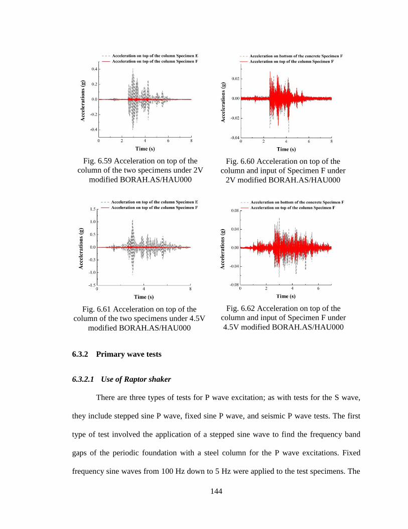
144
6.3.2 Primary wave tests
6.3.2.1 Use of Raptor shaker
There are three types of tests for P wave excitation; as with tests for the S wave,
they include stepped sine P wave, fixed sine P wave, and seismic P wave tests. The first
type of test involved the application of a stepped sine wave to find the frequency band
gaps of the periodic foundation with a steel column for the P wave excitations. Fixed
frequency sine waves from 100 Hz down to 5 Hz were applied to the test specimens. The
Fig. 6.59 Acceleration on top of the
column of the two specimens under 2V
modified BORAH.AS/HAU000
Fig. 6.60 Acceleration on top of the
column and input of Specimen F under
2V modified BORAH.AS/HAU000
Fig. 6.61 Acceleration on top of the
column of the two specimens under 4.5V
modified BORAH.AS/HAU000
Fig. 6.62 Acceleration on top of the
column and input of Specimen F under
4.5V modified BORAH.AS/HAU000
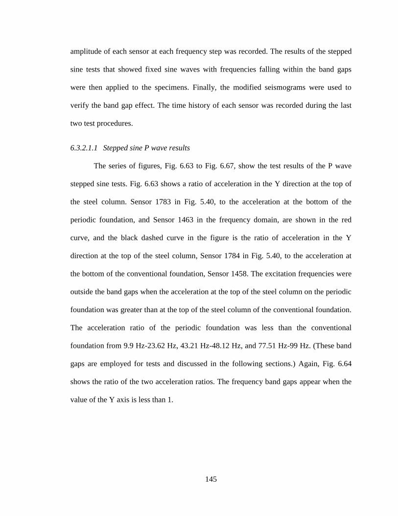
145
amplitude of each sensor at each frequency step was recorded. The results of the stepped
sine tests that showed fixed sine waves with frequencies falling within the band gaps
were then applied to the specimens. Finally, the modified seismograms were used to
verify the band gap effect. The time history of each sensor was recorded during the last
two test procedures.
6.3.2.1.1 Stepped sine P wave results
The series of figures, Fig. 6.63 to Fig. 6.67, show the test results of the P wave
stepped sine tests. Fig. 6.63 shows a ratio of acceleration in the Y direction at the top of
the steel column. Sensor 1783 in Fig. 5.40, to the acceleration at the bottom of the
periodic foundation, and Sensor 1463 in the frequency domain, are shown in the red
curve, and the black dashed curve in the figure is the ratio of acceleration in the Y
direction at the top of the steel column, Sensor 1784 in Fig. 5.40, to the acceleration at
the bottom of the conventional foundation, Sensor 1458. The excitation frequencies were
outside the band gaps when the acceleration at the top of the steel column on the periodic
foundation was greater than at the top of the steel column of the conventional foundation.
The acceleration ratio of the periodic foundation was less than the conventional
foundation from 9.9 Hz-23.62 Hz, 43.21 Hz-48.12 Hz, and 77.51 Hz-99 Hz. (These band
gaps are employed for tests and discussed in the following sections.) Again, Fig. 6.64
shows the ratio of the two acceleration ratios. The frequency band gaps appear when the
value of the Y axis is less than 1.
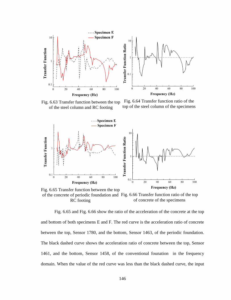
146
Fig. 6.65 and Fig. 6.66 show the ratio of the acceleration of the concrete at the top
and bottom of both specimens E and F. The red curve is the acceleration ratio of concrete
between the top, Sensor 1780, and the bottom, Sensor 1463, of the periodic foundation.
The black dashed curve shows the acceleration ratio of concrete between the top, Sensor
1461, and the bottom, Sensor 1458, of the conventional founation in the frequency
domain. When the value of the red curve was less than the black dashed curve, the input
Fig. 6.63 Transfer function between the top
of the steel column and RC footing
Fig. 6.64 Transfer function ratio of the
top of the steel column of the specimens
Fig. 6.65 Transfer function between the top
of the concrete of periodic foundation and
RC footing
Fig. 6.66 Transfer function ratio of the top
of concrete of the specimens

147
P wave was mitigated. The ranges of the band gap are 11.86 Hz-14.8 Hz, 16.76 Hz-23.61
Hz, 27.54 Hz-43.21 Hz, 47.13 Hz-48 Hz, 51.5 Hz-53 Hz, and 81.43 Hz-86.33 Hz. Fig.
6.66 shows the ratio of the transfer function of the two specimens.
6.3.2.1.2 Fixed sine P wave results
Harmonic P wave excitation was applied to the specimens, and their frequencies
were found to be in the range of the band gaps, i.e., 21.2 Hz, according to the results of
the stepped sine tests in Section 6.3.2.1.1. The range of figures, Fig. 6.67 to Fig. 6.69,
shows acceleration in the Y direction under a sine P wave of 21.2 Hz. The red curve in
Fig. 6.67 is the acceleration at the top of the steel column with the periodic foundation,
Sensor 1783. The dashed gray curve is the acceleration response at the top of the steel
column with the conventional foundation, Sensor 1784. Fig. 6.67 shows that, at the
beginning of the harmonic motion, the two curves have nearly the same peak acceleration
owing to the transient effect; when the specimen was in the steady state, the peak
acceleration, 0.0479 from Sensor 1783, at the top of the steel column on the periodic
foundation, was 63.9% that of the conventional foundation, 0.073g from Sensor 1784.
Fig. 6.68 shows the acceleration at the top of the concrete in specimens E and F. The
acceleration at the top of the concrete of Specimen F, 0.029g from Sensor 1780, was
51.8% that of Specimen E, 0.056g from Sensor 1461. Fig. 6.69 shows the acceleration in
concrete located in the 3rd row from the bottom of the periodic foundation under the
harmonic P waves of 21.2 Hz. When the specimen was in the steady state, the peak
acceleration, 0.03g from Sensor 1779 at the intersection between the third and fourth unit
cells in the periodic foundation, to be 60% of the conventional foundation, 0.05g from
Sensor 1459.
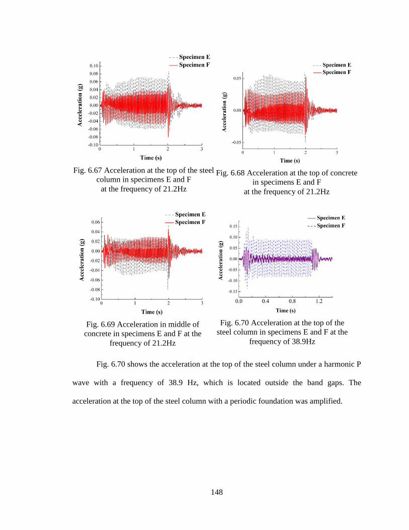
148
Fig. 6.70 shows the acceleration at the top of the steel column under a harmonic P
wave with a frequency of 38.9 Hz, which is located outside the band gaps. The
acceleration at the top of the steel column with a periodic foundation was amplified.
Fig. 6.67 Acceleration at the top of the steel
column in specimens E and F
at the frequency of 21.2Hz
Fig. 6.68 Acceleration at the top of concrete
in specimens E and F
at the frequency of 21.2Hz
Fig. 6.69 Acceleration in middle of
concrete in specimens E and F at the
frequency of 21.2Hz
Fig. 6.70 Acceleration at the top of the
steel column in specimens E and F at the
frequency of 38.9Hz
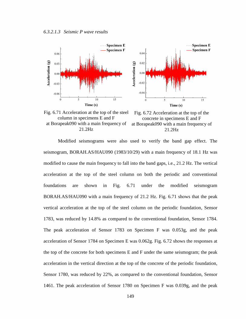
149
6.3.2.1.3 Seismic P wave results
Modified seismograms were also used to verify the band gap effect. The
seismogram, BORAH.AS/HAU090 (1983/10/29) with a main frequency of 18.1 Hz was
modified to cause the main frequency to fall into the band gaps, i.e., 21.2 Hz. The vertical
acceleration at the top of the steel column on both the periodic and conventional
foundations are shown in Fig. 6.71 under the modified seismogram
BORAH.AS/HAU090 with a main frequency of 21.2 Hz. Fig. 6.71 shows that the peak
vertical acceleration at the top of the steel column on the periodic foundation, Sensor
1783, was reduced by 14.8% as compared to the conventional foundation, Sensor 1784.
The peak acceleration of Sensor 1783 on Specimen F was 0.053g, and the peak
acceleration of Sensor 1784 on Specimen E was 0.062g. Fig. 6.72 shows the responses at
the top of the concrete for both specimens E and F under the same seismogram; the peak
acceleration in the vertical direction at the top of the concrete of the periodic foundation,
Sensor 1780, was reduced by 22%, as compared to the conventional foundation, Sensor
1461. The peak acceleration of Sensor 1780 on Specimen F was 0.039g, and the peak
Fig. 6.71 Acceleration at the top of the steel
column in specimens E and F
at Borapeak090 with a main frequency of
21.2Hz
Fig. 6.72 Acceleration at the top of the
concrete in specimens E and F
at Borapeak090 with a main frequency of
21.2Hz
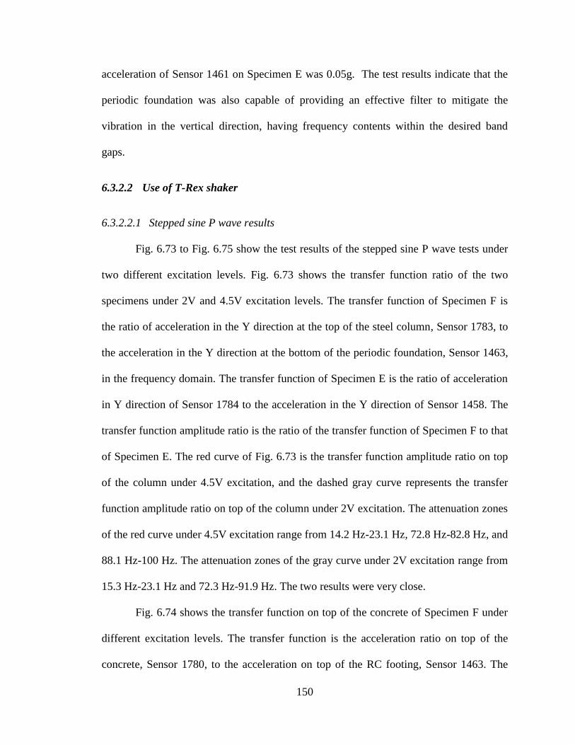
150
acceleration of Sensor 1461 on Specimen E was 0.05g. The test results indicate that the
periodic foundation was also capable of providing an effective filter to mitigate the
vibration in the vertical direction, having frequency contents within the desired band
gaps.
6.3.2.2 Use of T-Rex shaker
6.3.2.2.1 Stepped sine P wave results
Fig. 6.73 to Fig. 6.75 show the test results of the stepped sine P wave tests under
two different excitation levels. Fig. 6.73 shows the transfer function ratio of the two
specimens under 2V and 4.5V excitation levels. The transfer function of Specimen F is
the ratio of acceleration in the Y direction at the top of the steel column, Sensor 1783, to
the acceleration in the Y direction at the bottom of the periodic foundation, Sensor 1463,
in the frequency domain. The transfer function of Specimen E is the ratio of acceleration
in Y direction of Sensor 1784 to the acceleration in the Y direction of Sensor 1458. The
transfer function amplitude ratio is the ratio of the transfer function of Specimen F to that
of Specimen E. The red curve of Fig. 6.73 is the transfer function amplitude ratio on top
of the column under 4.5V excitation, and the dashed gray curve represents the transfer
function amplitude ratio on top of the column under 2V excitation. The attenuation zones
of the red curve under 4.5V excitation range from 14.2 Hz-23.1 Hz, 72.8 Hz-82.8 Hz, and
88.1 Hz-100 Hz. The attenuation zones of the gray curve under 2V excitation range from
15.3 Hz-23.1 Hz and 72.3 Hz-91.9 Hz. The two results were very close.
Fig. 6.74 shows the transfer function on top of the concrete of Specimen F under
different excitation levels. The transfer function is the acceleration ratio on top of the
concrete, Sensor 1780, to the acceleration on top of the RC footing, Sensor 1463. The
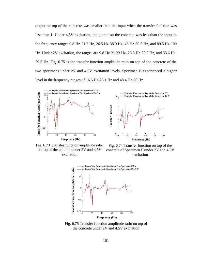
151
output on top of the concrete was smaller than the input when the transfer function was
less than 1. Under 4.5V excitation, the output on the concrete was less than the input in
the frequency ranges 9.8 Hz-21.2 Hz, 26.5 Hz-38.9 Hz, 48 Hz-60.5 Hz, and 89.5 Hz-100
Hz. Under 2V excitation, the ranges are 9.8 Hz-21.23 Hz, 26.5 Hz-39.8 Hz, and 55.6 Hz-
79.5 Hz. Fig. 6.75 is the transfer function amplitude ratio on top of the concrete of the
two specimens under 2V and 4.5V excitation levels. Specimen E experienced a higher
level in the frequency ranges of 16.5 Hz-23.1 Hz and 48.4 Hz-60 Hz.
Fig. 6.73 Transfer function amplitude ratio
on top of the column under 2V and 4.5V
excitation
Fig. 6.74 Transfer function on top of the
concrete of Specimen F under 2V and 4.5V
excitation
Fig. 6.75 Transfer function amplitude ratio on top of
the concrete under 2V and 4.5V excitation
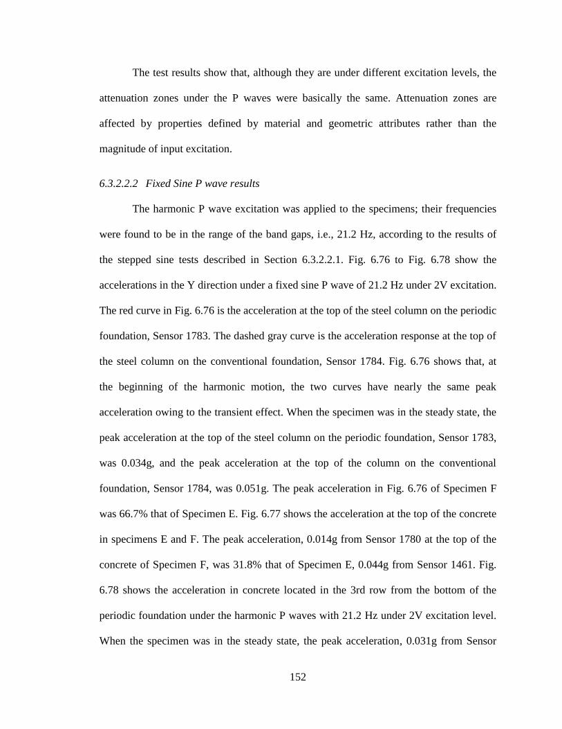
152
The test results show that, although they are under different excitation levels, the
attenuation zones under the P waves were basically the same. Attenuation zones are
affected by properties defined by material and geometric attributes rather than the
magnitude of input excitation.
6.3.2.2.2 Fixed Sine P wave results
The harmonic P wave excitation was applied to the specimens; their frequencies
were found to be in the range of the band gaps, i.e., 21.2 Hz, according to the results of
the stepped sine tests described in Section 6.3.2.2.1. Fig. 6.76 to Fig. 6.78 show the
accelerations in the Y direction under a fixed sine P wave of 21.2 Hz under 2V excitation.
The red curve in Fig. 6.76 is the acceleration at the top of the steel column on the periodic
foundation, Sensor 1783. The dashed gray curve is the acceleration response at the top of
the steel column on the conventional foundation, Sensor 1784. Fig. 6.76 shows that, at
the beginning of the harmonic motion, the two curves have nearly the same peak
acceleration owing to the transient effect. When the specimen was in the steady state, the
peak acceleration at the top of the steel column on the periodic foundation, Sensor 1783,
was 0.034g, and the peak acceleration at the top of the column on the conventional
foundation, Sensor 1784, was 0.051g. The peak acceleration in Fig. 6.76 of Specimen F
was 66.7% that of Specimen E. Fig. 6.77 shows the acceleration at the top of the concrete
in specimens E and F. The peak acceleration, 0.014g from Sensor 1780 at the top of the
concrete of Specimen F, was 31.8% that of Specimen E, 0.044g from Sensor 1461. Fig.
6.78 shows the acceleration in concrete located in the 3rd row from the bottom of the
periodic foundation under the harmonic P waves with 21.2 Hz under 2V excitation level.
When the specimen was in the steady state, the peak acceleration, 0.031g from Sensor
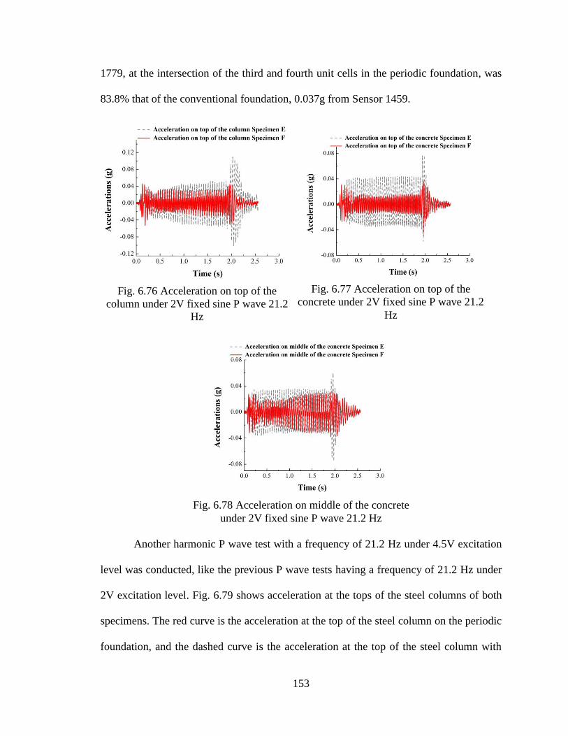
153
1779, at the intersection of the third and fourth unit cells in the periodic foundation, was
83.8% that of the conventional foundation, 0.037g from Sensor 1459.
Another harmonic P wave test with a frequency of 21.2 Hz under 4.5V excitation
level was conducted, like the previous P wave tests having a frequency of 21.2 Hz under
2V excitation level. Fig. 6.79 shows acceleration at the tops of the steel columns of both
specimens. The red curve is the acceleration at the top of the steel column on the periodic
foundation, and the dashed curve is the acceleration at the top of the steel column with
Fig. 6.76 Acceleration on top of the
column under 2V fixed sine P wave 21.2
Hz
Fig. 6.77 Acceleration on top of the
concrete under 2V fixed sine P wave 21.2
Hz
Fig. 6.78 Acceleration on middle of the concrete
under 2V fixed sine P wave 21.2 Hz
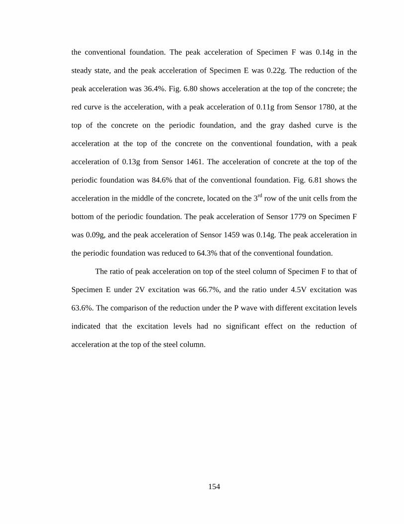
154
the conventional foundation. The peak acceleration of Specimen F was 0.14g in the
steady state, and the peak acceleration of Specimen E was 0.22g. The reduction of the
peak acceleration was 36.4%. Fig. 6.80 shows acceleration at the top of the concrete; the
red curve is the acceleration, with a peak acceleration of 0.11g from Sensor 1780, at the
top of the concrete on the periodic foundation, and the gray dashed curve is the
acceleration at the top of the concrete on the conventional foundation, with a peak
acceleration of 0.13g from Sensor 1461. The acceleration of concrete at the top of the
periodic foundation was 84.6% that of the conventional foundation. Fig. 6.81 shows the
acceleration in the middle of the concrete, located on the 3rd
row of the unit cells from the
bottom of the periodic foundation. The peak acceleration of Sensor 1779 on Specimen F
was 0.09g, and the peak acceleration of Sensor 1459 was 0.14g. The peak acceleration in
the periodic foundation was reduced to 64.3% that of the conventional foundation.
The ratio of peak acceleration on top of the steel column of Specimen F to that of
Specimen E under 2V excitation was 66.7%, and the ratio under 4.5V excitation was
63.6%. The comparison of the reduction under the P wave with different excitation levels
indicated that the excitation levels had no significant effect on the reduction of
acceleration at the top of the steel column.
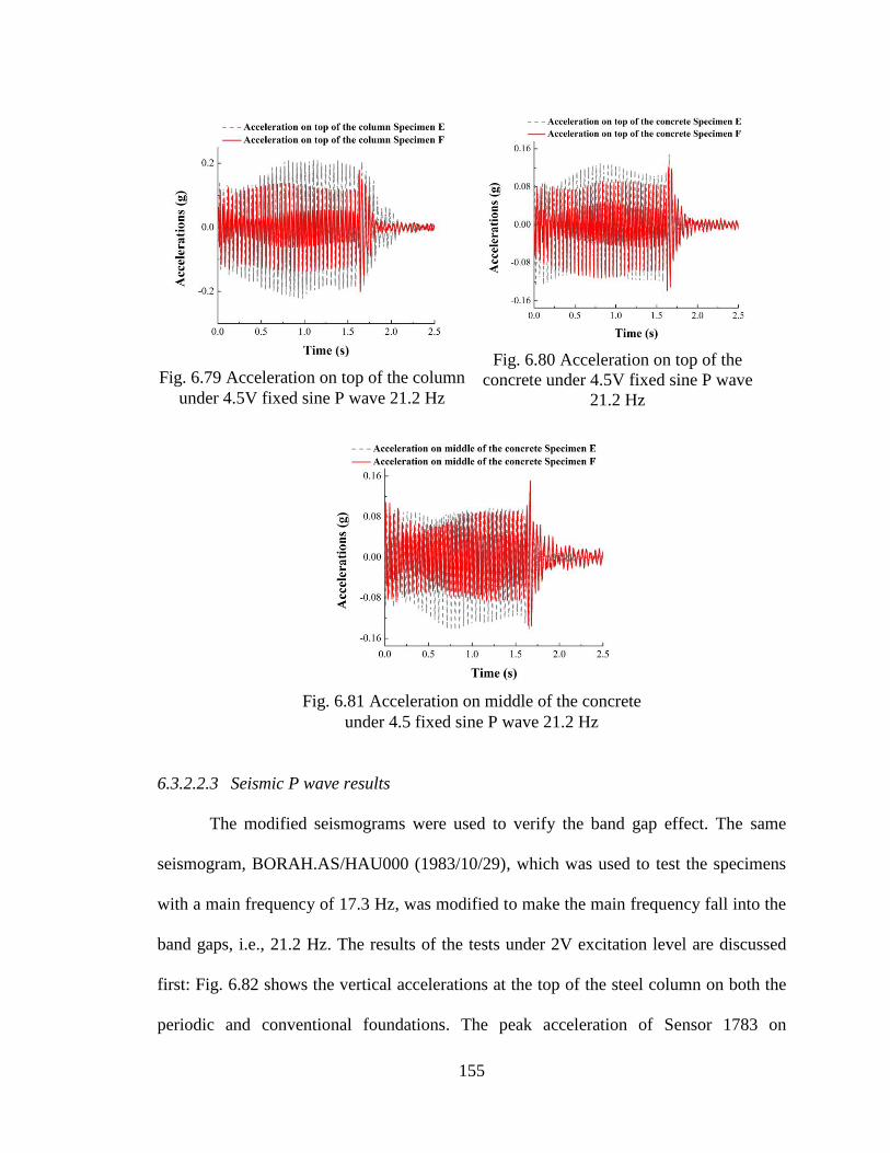
155
6.3.2.2.3 Seismic P wave results
The modified seismograms were used to verify the band gap effect. The same
seismogram, BORAH.AS/HAU000 (1983/10/29), which was used to test the specimens
with a main frequency of 17.3 Hz, was modified to make the main frequency fall into the
band gaps, i.e., 21.2 Hz. The results of the tests under 2V excitation level are discussed
first: Fig. 6.82 shows the vertical accelerations at the top of the steel column on both the
periodic and conventional foundations. The peak acceleration of Sensor 1783 on
Fig. 6.79 Acceleration on top of the column
under 4.5V fixed sine P wave 21.2 Hz
Fig. 6.80 Acceleration on top of the
concrete under 4.5V fixed sine P wave
21.2 Hz
Fig. 6.81 Acceleration on middle of the concrete
under 4.5 fixed sine P wave 21.2 Hz
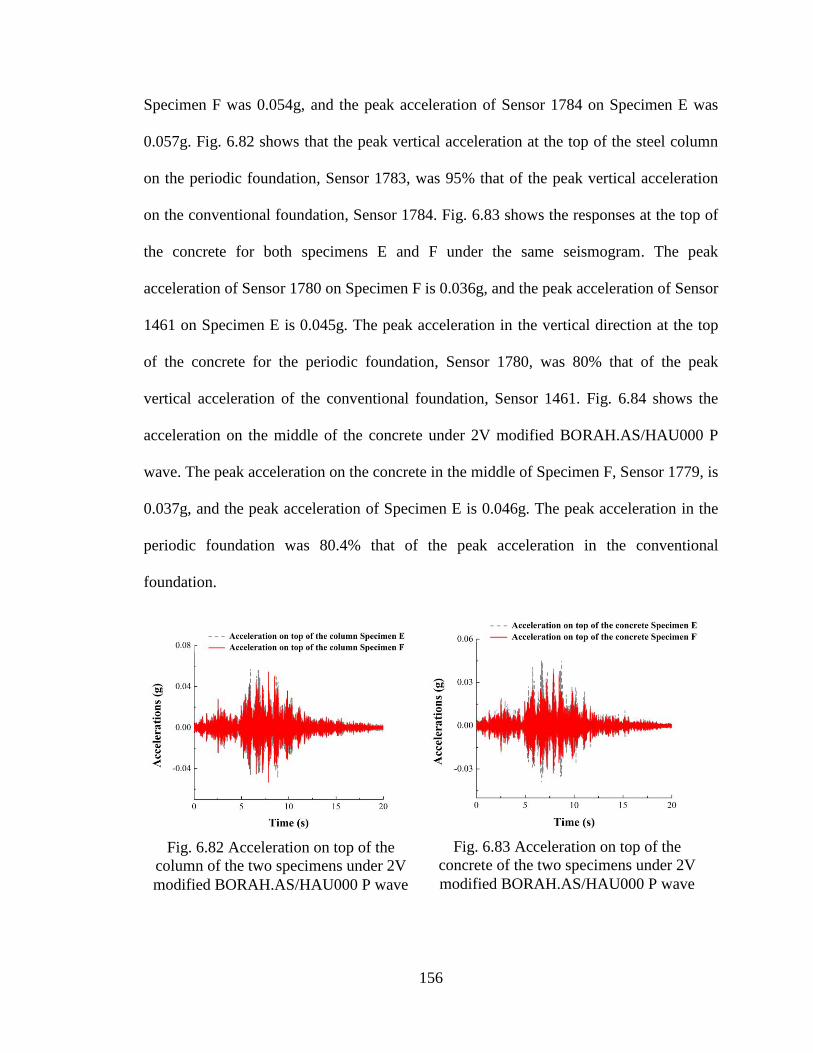
156
Specimen F was 0.054g, and the peak acceleration of Sensor 1784 on Specimen E was
0.057g. Fig. 6.82 shows that the peak vertical acceleration at the top of the steel column
on the periodic foundation, Sensor 1783, was 95% that of the peak vertical acceleration
on the conventional foundation, Sensor 1784. Fig. 6.83 shows the responses at the top of
the concrete for both specimens E and F under the same seismogram. The peak
acceleration of Sensor 1780 on Specimen F is 0.036g, and the peak acceleration of Sensor
1461 on Specimen E is 0.045g. The peak acceleration in the vertical direction at the top
of the concrete for the periodic foundation, Sensor 1780, was 80% that of the peak
vertical acceleration of the conventional foundation, Sensor 1461. Fig. 6.84 shows the
acceleration on the middle of the concrete under 2V modified BORAH.AS/HAU000 P
wave. The peak acceleration on the concrete in the middle of Specimen F, Sensor 1779, is
0.037g, and the peak acceleration of Specimen E is 0.046g. The peak acceleration in the
periodic foundation was 80.4% that of the peak acceleration in the conventional
foundation.
Fig. 6.82 Acceleration on top of the
column of the two specimens under 2V
modified BORAH.AS/HAU000 P wave
Fig. 6.83 Acceleration on top of the
concrete of the two specimens under 2V
modified BORAH.AS/HAU000 P wave
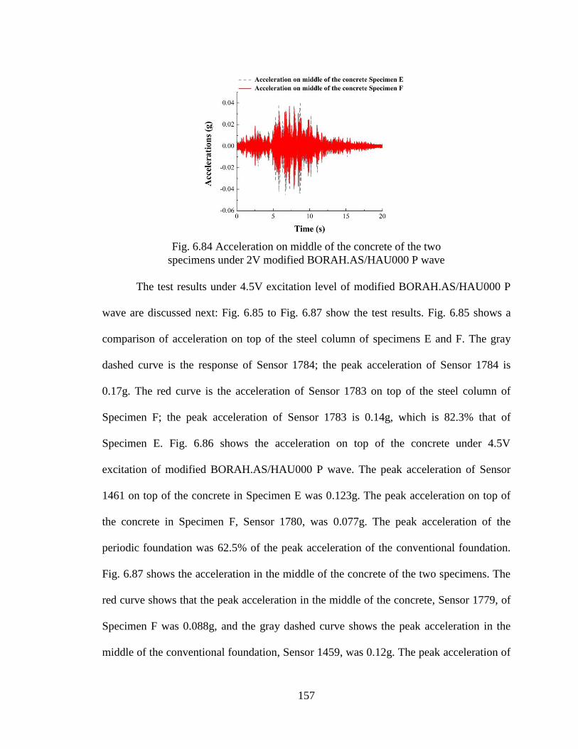
157
The test results under 4.5V excitation level of modified BORAH.AS/HAU000 P
wave are discussed next: Fig. 6.85 to Fig. 6.87 show the test results. Fig. 6.85 shows a
comparison of acceleration on top of the steel column of specimens E and F. The gray
dashed curve is the response of Sensor 1784; the peak acceleration of Sensor 1784 is
0.17g. The red curve is the acceleration of Sensor 1783 on top of the steel column of
Specimen F; the peak acceleration of Sensor 1783 is 0.14g, which is 82.3% that of
Specimen E. Fig. 6.86 shows the acceleration on top of the concrete under 4.5V
excitation of modified BORAH.AS/HAU000 P wave. The peak acceleration of Sensor
1461 on top of the concrete in Specimen E was 0.123g. The peak acceleration on top of
the concrete in Specimen F, Sensor 1780, was 0.077g. The peak acceleration of the
periodic foundation was 62.5% of the peak acceleration of the conventional foundation.
Fig. 6.87 shows the acceleration in the middle of the concrete of the two specimens. The
red curve shows that the peak acceleration in the middle of the concrete, Sensor 1779, of
Specimen F was 0.088g, and the gray dashed curve shows the peak acceleration in the
middle of the conventional foundation, Sensor 1459, was 0.12g. The peak acceleration of
Fig. 6.84 Acceleration on middle of the concrete of the two
specimens under 2V modified BORAH.AS/HAU000 P wave
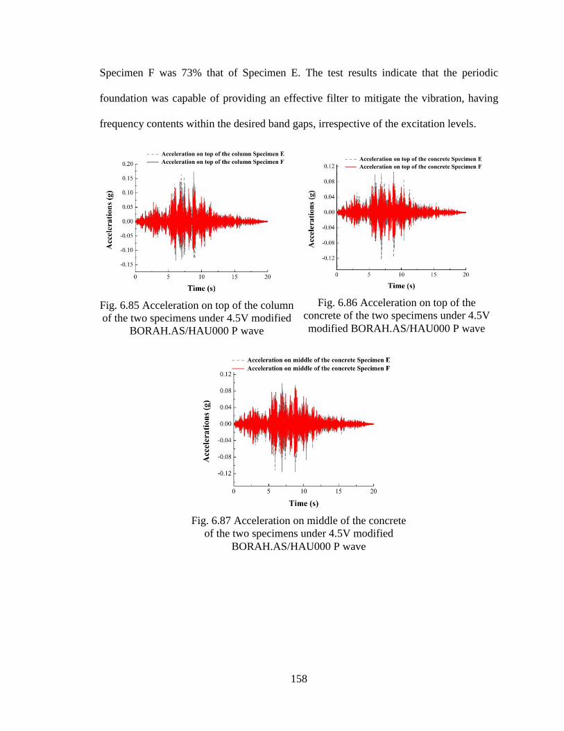
158
Specimen F was 73% that of Specimen E. The test results indicate that the periodic
foundation was capable of providing an effective filter to mitigate the vibration, having
frequency contents within the desired band gaps, irrespective of the excitation levels.
Fig. 6.85 Acceleration on top of the column
of the two specimens under 4.5V modified
BORAH.AS/HAU000 P wave
Fig. 6.86 Acceleration on top of the
concrete of the two specimens under 4.5V
modified BORAH.AS/HAU000 P wave
Fig. 6.87 Acceleration on middle of the concrete
of the two specimens under 4.5V modified
BORAH.AS/HAU000 P wave
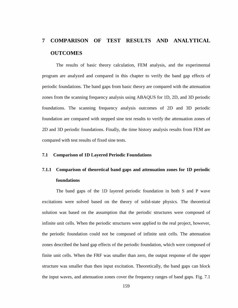
159
7 COMPARISON OF TEST RESULTS AND ANALYTICAL
OUTCOMES
The results of basic theory calculation, FEM analysis, and the experimental
program are analyzed and compared in this chapter to verify the band gap effects of
periodic foundations. The band gaps from basic theory are compared with the attenuation
zones from the scanning frequency analysis using ABAQUS for 1D, 2D, and 3D periodic
foundations. The scanning frequency analysis outcomes of 2D and 3D periodic
foundation are compared with stepped sine test results to verify the attenuation zones of
2D and 3D periodic foundations. Finally, the time history analysis results from FEM are
compared with test results of fixed sine tests.
7.1 Comparison of 1D Layered Periodic Foundations
7.1.1 Comparison of theoretical band gaps and attenuation zones for 1D periodic
foundations
The band gaps of the 1D layered periodic foundation in both S and P wave
excitations were solved based on the theory of solid-state physics. The theoretical
solution was based on the assumption that the periodic structures were composed of
infinite unit cells. When the periodic structures were applied to the real project, however,
the periodic foundation could not be composed of infinite unit cells. The attenuation
zones described the band gap effects of the periodic foundation, which were composed of
finite unit cells. When the FRF was smaller than zero, the output response of the upper
structure was smaller than then input excitation. Theoretically, the band gaps can block
the input waves, and attenuation zones cover the frequency ranges of band gaps. Fig. 7.1
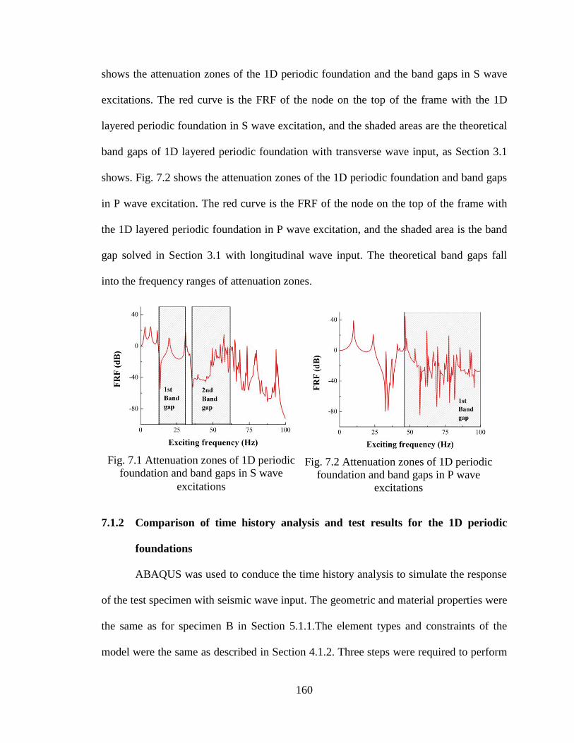
160
shows the attenuation zones of the 1D periodic foundation and the band gaps in S wave
excitations. The red curve is the FRF of the node on the top of the frame with the 1D
layered periodic foundation in S wave excitation, and the shaded areas are the theoretical
band gaps of 1D layered periodic foundation with transverse wave input, as Section 3.1
shows. Fig. 7.2 shows the attenuation zones of the 1D periodic foundation and band gaps
in P wave excitation. The red curve is the FRF of the node on the top of the frame with
the 1D layered periodic foundation in P wave excitation, and the shaded area is the band
gap solved in Section 3.1 with longitudinal wave input. The theoretical band gaps fall
into the frequency ranges of attenuation zones.
7.1.2 Comparison of time history analysis and test results for the 1D periodic
foundations
ABAQUS was used to conduce the time history analysis to simulate the response
of the test specimen with seismic wave input. The geometric and material properties were
the same as for specimen B in Section 5.1.1.The element types and constraints of the
model were the same as described in Section 4.1.2. Three steps were required to perform
Fig. 7.1 Attenuation zones of 1D periodic
foundation and band gaps in S wave
excitations
Fig. 7.2 Attenuation zones of 1D periodic
foundation and band gaps in P wave
excitations
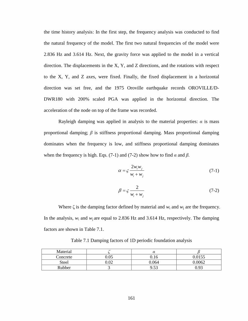
161
the time history analysis: In the first step, the frequency analysis was conducted to find
the natural frequency of the model. The first two natural frequencies of the model were
2.836 Hz and 3.614 Hz. Next, the gravity force was applied to the model in a vertical
direction. The displacements in the X, Y, and Z directions, and the rotations with respect
to the X, Y, and Z axes, were fixed. Finally, the fixed displacement in a horizontal
direction was set free, and the 1975 Oroville earthquake records OROVILLE/D-
DWR180 with 200% scaled PGA was applied in the horizontal direction. The
acceleration of the node on top of the frame was recorded.
Rayleigh damping was applied in analysis to the material properties: α is mass
proportional damping; β is stiffness proportional damping. Mass proportional damping
dominates when the frequency is low, and stiffness proportional damping dominates
when the frequency is high. Eqs. (7-1) and (7-2) show how to find α and β.
(7-1)
(7-2)
Where ζ is the damping factor defined by material and wi and wj are the frequency.
In the analysis, wi and wj are equal to 2.836 Hz and 3.614 Hz, respectively. The damping
factors are shown in Table 7.1.
Table 7.1 Damping factors of 1D periodic foundation analysis
Material ζ α β
Concrete 0.05 0.16 0.0155
Steel 0.02 0.064 0.0062
Rubber 3 9.53 0.93
2 i j
i j
w w
w w
2
i jw w
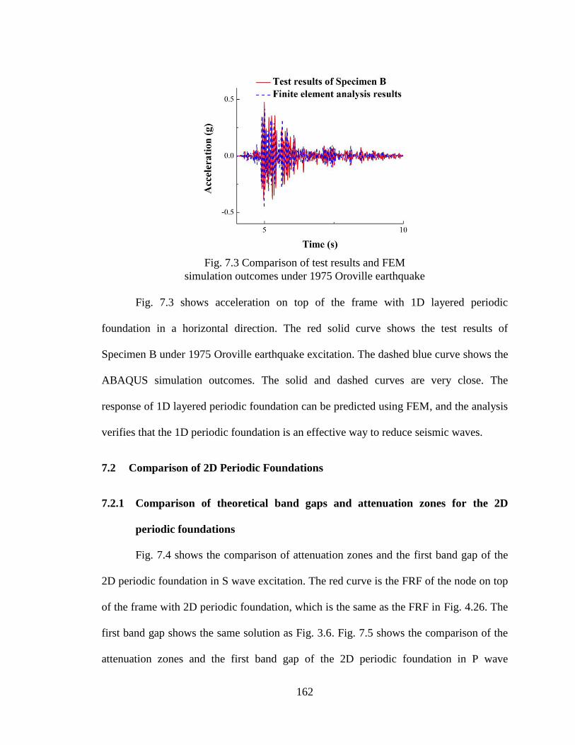
162
Fig. 7.3 shows acceleration on top of the frame with 1D layered periodic
foundation in a horizontal direction. The red solid curve shows the test results of
Specimen B under 1975 Oroville earthquake excitation. The dashed blue curve shows the
ABAQUS simulation outcomes. The solid and dashed curves are very close. The
response of 1D layered periodic foundation can be predicted using FEM, and the analysis
verifies that the 1D periodic foundation is an effective way to reduce seismic waves.
7.2 Comparison of 2D Periodic Foundations
7.2.1 Comparison of theoretical band gaps and attenuation zones for the 2D
periodic foundations
Fig. 7.4 shows the comparison of attenuation zones and the first band gap of the
2D periodic foundation in S wave excitation. The red curve is the FRF of the node on top
of the frame with 2D periodic foundation, which is the same as the FRF in Fig. 4.26. The
first band gap shows the same solution as Fig. 3.6. Fig. 7.5 shows the comparison of the
attenuation zones and the first band gap of the 2D periodic foundation in P wave
Fig. 7.3 Comparison of test results and FEM
simulation outcomes under 1975 Oroville earthquake
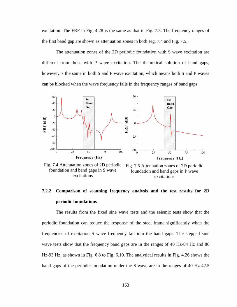
163
excitation. The FRF in Fig. 4.28 is the same as that in Fig. 7.5. The frequency ranges of
the first band gap are shown as attenuation zones in both Fig. 7.4 and Fig. 7.5.
The attenuation zones of the 2D periodic foundation with S wave excitation are
different from those with P wave excitation. The theoretical solution of band gaps,
however, is the same in both S and P wave excitation, which means both S and P waves
can be blocked when the wave frequency falls in the frequency ranges of band gaps.
7.2.2 Comparison of scanning frequency analysis and the test results for 2D
periodic foundations
The results from the fixed sine wave tests and the seismic tests show that the
periodic foundation can reduce the response of the steel frame significantly when the
frequencies of excitation S wave frequency fall into the band gaps. The stepped sine
wave tests show that the frequency band gaps are in the ranges of 40 Hz-84 Hz and 86
Hz-93 Hz, as shown in Fig. 6.8 to Fig. 6.10. The analytical results in Fig. 4.26 shows the
band gaps of the periodic foundation under the S wave are in the ranges of 40 Hz-42.5
Fig. 7.4 Attenuation zones of 2D periodic
foundation and band gaps in S wave
excitations
Fig. 7.5 Attenuation zones of 2D periodic
foundation and band gaps in P wave
excitations
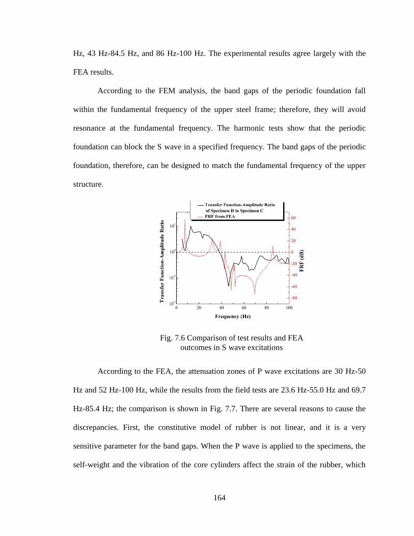
164
Hz, 43 Hz-84.5 Hz, and 86 Hz-100 Hz. The experimental results agree largely with the
FEA results.
According to the FEM analysis, the band gaps of the periodic foundation fall
within the fundamental frequency of the upper steel frame; therefore, they will avoid
resonance at the fundamental frequency. The harmonic tests show that the periodic
foundation can block the S wave in a specified frequency. The band gaps of the periodic
foundation, therefore, can be designed to match the fundamental frequency of the upper
structure.
According to the FEA, the attenuation zones of P wave excitations are 30 Hz-50
Hz and 52 Hz-100 Hz, while the results from the field tests are 23.6 Hz-55.0 Hz and 69.7
Hz-85.4 Hz; the comparison is shown in Fig. 7.7. There are several reasons to cause the
discrepancies. First, the constitutive model of rubber is not linear, and it is a very
sensitive parameter for the band gaps. When the P wave is applied to the specimens, the
self-weight and the vibration of the core cylinders affect the strain of the rubber, which
Fig. 7.6 Comparison of test results and FEA
outcomes in S wave excitations
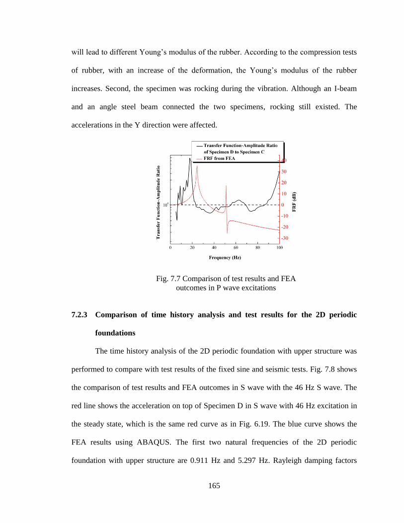
165
will lead to different Young’s modulus of the rubber. According to the compression tests
of rubber, with an increase of the deformation, the Young’s modulus of the rubber
increases. Second, the specimen was rocking during the vibration. Although an I-beam
and an angle steel beam connected the two specimens, rocking still existed. The
accelerations in the Y direction were affected.
7.2.3 Comparison of time history analysis and test results for the 2D periodic
foundations
The time history analysis of the 2D periodic foundation with upper structure was
performed to compare with test results of the fixed sine and seismic tests. Fig. 7.8 shows
the comparison of test results and FEA outcomes in S wave with the 46 Hz S wave. The
red line shows the acceleration on top of Specimen D in S wave with 46 Hz excitation in
the steady state, which is the same red curve as in Fig. 6.19. The blue curve shows the
FEA results using ABAQUS. The first two natural frequencies of the 2D periodic
foundation with upper structure are 0.911 Hz and 5.297 Hz. Rayleigh damping factors
Fig. 7.7 Comparison of test results and FEA
outcomes in P wave excitations
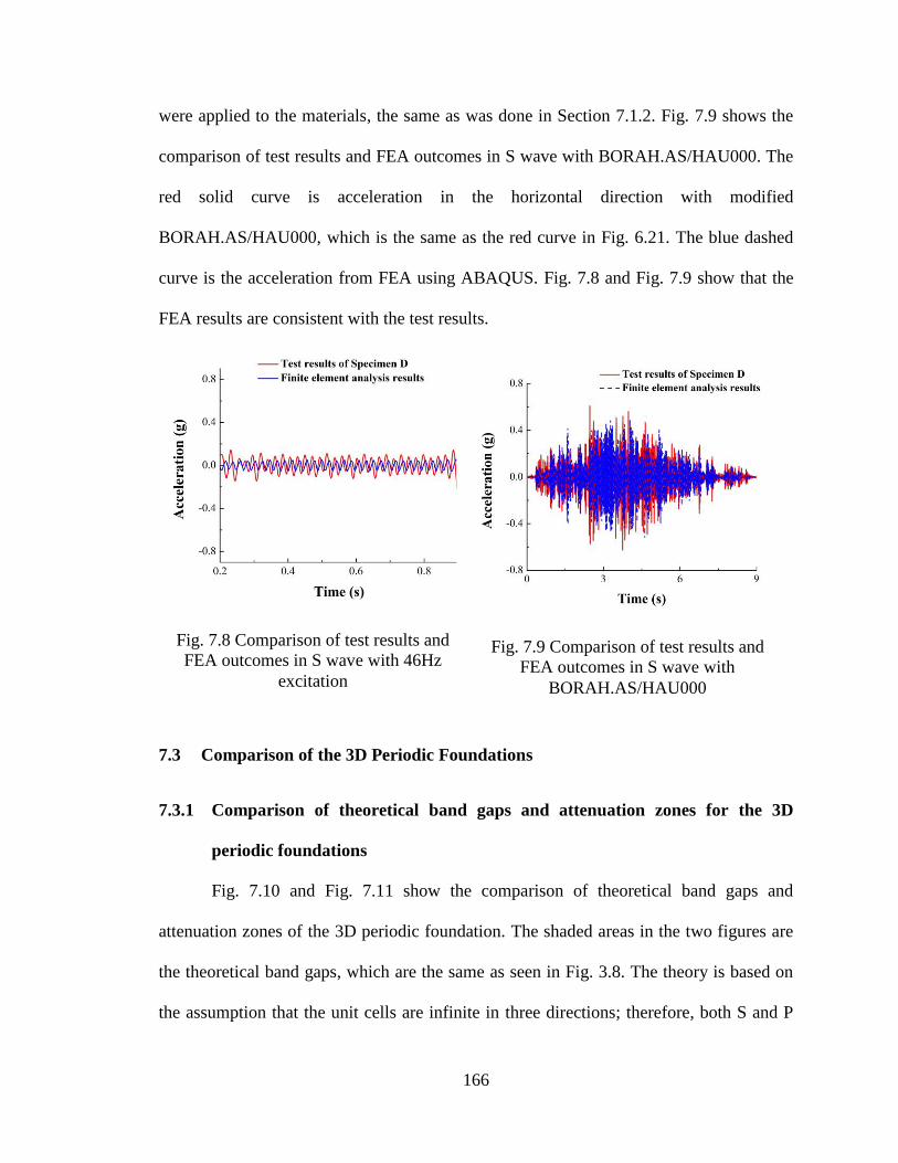
166
were applied to the materials, the same as was done in Section 7.1.2. Fig. 7.9 shows the
comparison of test results and FEA outcomes in S wave with BORAH.AS/HAU000. The
red solid curve is acceleration in the horizontal direction with modified
BORAH.AS/HAU000, which is the same as the red curve in Fig. 6.21. The blue dashed
curve is the acceleration from FEA using ABAQUS. Fig. 7.8 and Fig. 7.9 show that the
FEA results are consistent with the test results.
7.3 Comparison of the 3D Periodic Foundations
7.3.1 Comparison of theoretical band gaps and attenuation zones for the 3D
periodic foundations
Fig. 7.10 and Fig. 7.11 show the comparison of theoretical band gaps and
attenuation zones of the 3D periodic foundation. The shaded areas in the two figures are
the theoretical band gaps, which are the same as seen in Fig. 3.8. The theory is based on
the assumption that the unit cells are infinite in three directions; therefore, both S and P
Fig. 7.8 Comparison of test results and
FEA outcomes in S wave with 46Hz
excitation
Fig. 7.9 Comparison of test results and
FEA outcomes in S wave with
BORAH.AS/HAU000
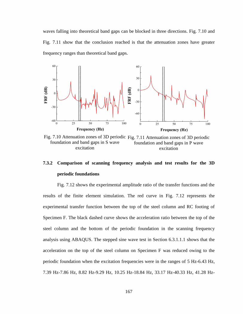
167
waves falling into theoretical band gaps can be blocked in three directions. Fig. 7.10 and
Fig. 7.11 show that the conclusion reached is that the attenuation zones have greater
frequency ranges than theoretical band gaps.
7.3.2 Comparison of scanning frequency analysis and test results for the 3D
periodic foundations
Fig. 7.12 shows the experimental amplitude ratio of the transfer functions and the
results of the finite element simulation. The red curve in Fig. 7.12 represents the
experimental transfer function between the top of the steel column and RC footing of
Specimen F. The black dashed curve shows the acceleration ratio between the top of the
steel column and the bottom of the periodic foundation in the scanning frequency
analysis using ABAQUS. The stepped sine wave test in Section 6.3.1.1.1 shows that the
acceleration on the top of the steel column on Specimen F was reduced owing to the
periodic foundation when the excitation frequencies were in the ranges of 5 Hz-6.43 Hz,
7.39 Hz-7.86 Hz, 8.82 Hz-9.29 Hz, 10.25 Hz-18.84 Hz, 33.17 Hz-40.33 Hz, 41.28 Hz-
Fig. 7.10 Attenuation zones of 3D periodic
foundation and band gaps in S wave
excitation
Fig. 7.11 Attenuation zones of 3D periodic
foundation and band gaps in P wave
excitation
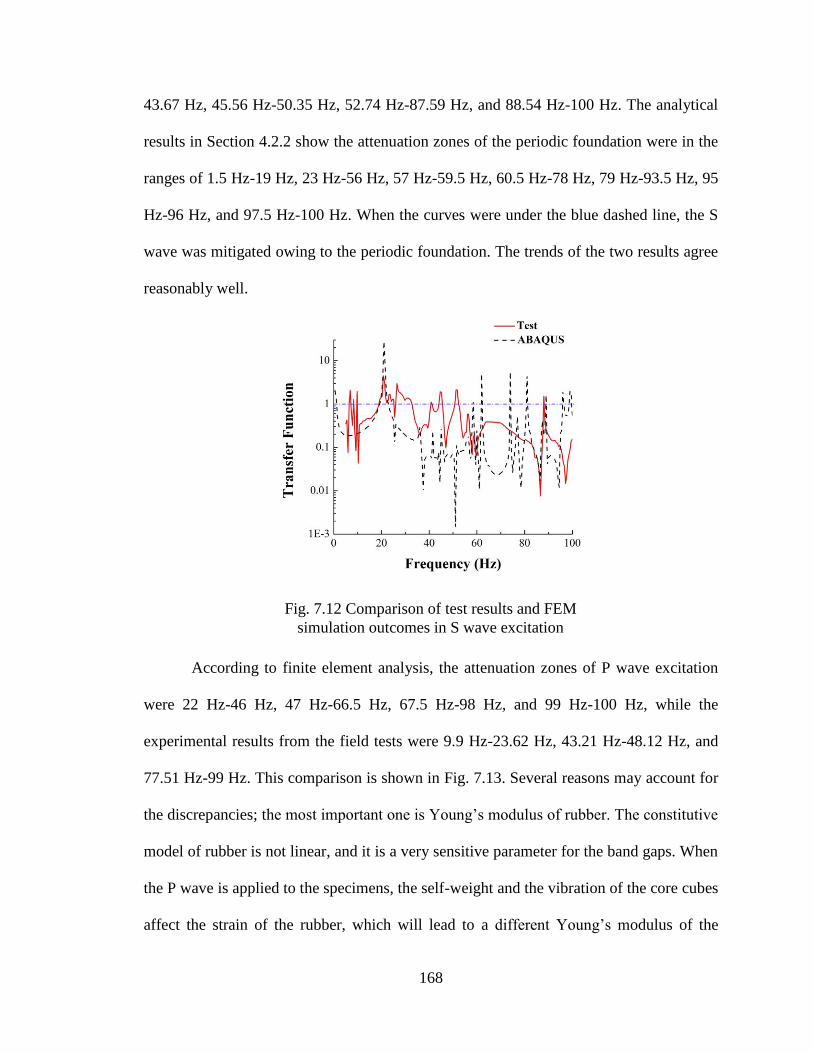
168
43.67 Hz, 45.56 Hz-50.35 Hz, 52.74 Hz-87.59 Hz, and 88.54 Hz-100 Hz. The analytical
results in Section 4.2.2 show the attenuation zones of the periodic foundation were in the
ranges of 1.5 Hz-19 Hz, 23 Hz-56 Hz, 57 Hz-59.5 Hz, 60.5 Hz-78 Hz, 79 Hz-93.5 Hz, 95
Hz-96 Hz, and 97.5 Hz-100 Hz. When the curves were under the blue dashed line, the S
wave was mitigated owing to the periodic foundation. The trends of the two results agree
reasonably well.
According to finite element analysis, the attenuation zones of P wave excitation
were 22 Hz-46 Hz, 47 Hz-66.5 Hz, 67.5 Hz-98 Hz, and 99 Hz-100 Hz, while the
experimental results from the field tests were 9.9 Hz-23.62 Hz, 43.21 Hz-48.12 Hz, and
77.51 Hz-99 Hz. This comparison is shown in Fig. 7.13. Several reasons may account for
the discrepancies; the most important one is Young’s modulus of rubber. The constitutive
model of rubber is not linear, and it is a very sensitive parameter for the band gaps. When
the P wave is applied to the specimens, the self-weight and the vibration of the core cubes
affect the strain of the rubber, which will lead to a different Young’s modulus of the
Fig. 7.12 Comparison of test results and FEM
simulation outcomes in S wave excitation
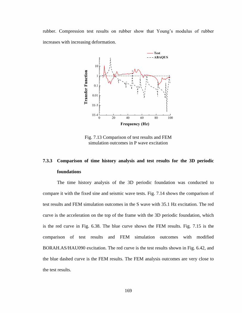
169
rubber. Compression test results on rubber show that Young’s modulus of rubber
increases with increasing deformation.
7.3.3 Comparison of time history analysis and test results for the 3D periodic
foundations
The time history analysis of the 3D periodic foundation was conducted to
compare it with the fixed sine and seismic wave tests. Fig. 7.14 shows the comparison of
test results and FEM simulation outcomes in the S wave with 35.1 Hz excitation. The red
curve is the acceleration on the top of the frame with the 3D periodic foundation, which
is the red curve in Fig. 6.38. The blue curve shows the FEM results. Fig. 7.15 is the
comparison of test results and FEM simulation outcomes with modified
BORAH.AS/HAU090 excitation. The red curve is the test results shown in Fig. 6.42, and
the blue dashed curve is the FEM results. The FEM analysis outcomes are very close to
the test results.
Fig. 7.13 Comparison of test results and FEM
simulation outcomes in P wave excitation
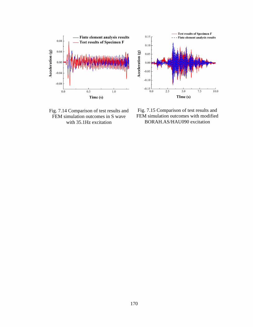
170
Fig. 7.14 Comparison of test results and
FEM simulation outcomes in S wave
with 35.1Hz excitation
Fig. 7.15 Comparison of test results and
FEM simulation outcomes with modified
BORAH.AS/HAU090 excitation
171
8 CONCLUSIONS AND SUGGESTIONS
8.1 Conclusions
The purpose of this research was to develop periodic foundations that mitigate or
change the pattern of earthquake energy before it reaches the foundation of structural
systems. The experimental programs were conducted to verify the band gap effects of
1D, 2D, and 3D periodic foundations. The following conclusions can be established from
this research:
(1) The solutions of frequency band gaps for 1D, 2D, and 3D periodic foundations
were obtained based on the theory of solid-state physics. The transfer matrix method,
plan wave equation method, and finite domain method can be used to solve the equation
of motion to find the theoretical band gaps of periodic foundations.
(2) FEM is an easy way to conduct the parametric studies and design the test
specimens for experimental programs on 1D, 2D, and 3D periodic foundations. Both
geometric and material properties were found to affect the band gaps of periodic
materials. Attenuation zones of the periodic foundation with the upper structure can be
found using scanning frequency analysis in ABAQUS.
(3) The feasibility of 1D, 2D, and 3D periodic foundations for structural vibration
isolation was verified experimentally. Shake table tests on the 1D periodic foundation
were conducted, including ambient vibration, seismogram tests, and harmonic tests. Field
tests were performed on the 2D and 3D periodic foundations. The stepped sine, fixed
sine, and seismic tests were performed to prove band gap effects.

172
(4) The test data showed that, when the main frequency of input wave falls into
the attenuation zones, the response of the upper structure can be reduced as compared to
the same structure without the periodic foundation. With different excitation levels, the
reductions of response on top of the column with the 3D periodic foundation are close.
(5) The FEA was conducted to compare with the test results in both the frequency
and time domains. The scanning frequency analysis was compared to the stepped sine
tests to find the attenuation zones; the time history analysis was compared to the fixed
sine and seismic tests. The FEA outcomes were close to the test results. FEM is an
effective way to predict the responses of periodic foundations.
8.2 Suggestions
The seismic isolation system based on periodic material is a new idea. Future
research in this area is suggested:
(1) Find wider and lower band gaps for seismic resistance; more factors need to
be considered, including topology of the unit cells, shape of core density, different types
of coating layer.
(2) Suggest nonlinear material properties of periodic foundations be studied. Until
now, only linear material properties have been considered based on the theory of periodic
structures, but the materials used for periodic foundations, i.e., rubber and reinforced
concrete, may have nonlinear behavior during earthquakes.
(3) A procedure is suggested as a way of studying design band gaps and bearing
capacity of periodic foundations that could lead to their design for different structures.
(4) An easy and cost-effective manufacturing procedure needs to be developed for
further application in construction projects.

173
174
9 REFERENCES
[1] Thomas, E. L., Gorishnyy, T., & Maldovan, M. (2006). Phononics: Colloidal
crystals go hypersonic. Nature Materials, 5(10), 773-774.
[2] Kelly, J. M. (1991). Base Isolation: Origins and Development. EERC News,
12(1), 1-3.
[3] See http://nees.buffalo.edu/seesl/a17.html for testing of elastomeric bearings.
[4] Kelly, J. M., & Naeim, F. (1999). Design of seismic isolated structures: From
theory to practice. Nueva York, John Wiley & Sons.
[5] Sayani, P. J., & Ryan, K. L. (2009). Evaluation of approaches to characterize
seismic isolation systems for design. Journal of Earthquake Engineering, 13(6), 835-851.
[6] Fulin, Z., Ping, Y., Qiaolin, X., Xiangyun, H., & Zhen, Y. (2006). Research and
application of seismic isolation system for building structures. Journal of Architecture
and Civil Engineering, 23(2), 1-8.
[7] Wilde, K., Gardoni, P., & Fujino, Y. (2000). Base isolation system with shape
memory alloy device for elevated highway bridges. Engineering Structures, 22(3), 222-
229.
[8] Kelly, J. M. (1986). Aseismic base isolation: review and bibliography. Soil
Dynamics and Earthquake Engineering, 5(4), 202-216.
[9] Zhou, F. L., Yang, Z., Liu, W. G., & Tan, P. (2004). New seismic isolation
system for irregular structure with the largest isolation building area in the world. In 13th
World Conference on Earthquake Engineering.
175
[10] Yang, Y.B., Lee, T.Y., Tsai, L.C. (1990). Response of multi-degree-of-freedom
structures with sliding supports. Earthquake Engineering and Structural Dynamics, 19(5)
739-752.
[11] Nanda, R. P., Agarwal, P., & Shrikhande, M. (2012). Base isolation system
suitable for masonry buildings. Asian Journal of Civil Engineering (Building and
Housing), 13(2), 195-202.
[12] Su, L., Ahmadi, G., & Tadjbakhsh, I. G. (1991). Performance of sliding resilient-
friction base-isolation system. Journal of Structural Engineering, 117(1), 165-181.
[13] Mostaghel, N., & Khodaverdian, M. (1987). Dynamics of resilient‐friction base
isolator (R‐FBI). Earthquake Engineering & Structural Dynamics, 15(3), 379-390.
[14] Su, L., Ahmadi, G., & Tadjbakhsh, I. G. (1991). Performance of sliding resilient-
friction base-isolation system. Journal of Structural Engineering, 117(1), 165-181.
[15] Kawamura, S., Kitazawa, K., Hisano, M., & Nagashima, I. (1988). Study of a
sliding-type base isolation system. System composition and element properties. In 9th.
WCEE. Japan.
[16] Komuro, T., Nishikawa, Y., Kimura, Y., & Isshiki, Y. (2005). Development and
realization of base isolation system for high-rise buildings. Journal of Advanced Concrete
Technology, 3(2), 233-239.
[17] Mokha, A., Constantinou, M. C., Reinhorn, A. M., & Zayas, V. A. (1991).
Experimental study of friction-pendulum isolation system. Journal of Structural
Engineering, 117(4), 1201-1217.
[18] See http://www.earthquakeprotection.com/benicia_martinez_bridge.html for
Benicia-Martinez Bridge Retrofit, California.
176
[19] Jangid, R. S., & Londhe, Y. B. (1998). Effectiveness of elliptical rolling rods for
base isolation. Journal of Structural Engineering, 124(4), 469-472.
[20] Nagarajaiah, S., Riley, M. A., & Reinhorn, A. (1993). Control of sliding-isolated
bridge with absolute acceleration feedback. Journal of Engineering Mechanics, 119(11),
2317-2332.
[21] Schmitendorf, W. E., Jabbari, F., & Yang, J. N. (1994). Robust control techniques
for buildings under earthquake excitation. Earthquake Engineering & Structural
Dynamics, 23(5), 539-552.
[22] Yang, J. N., Wu, J. C., Reinhorn, A. M., & Riley, M. (1996). Control of sliding-
isolated buildings using sliding-mode control. Journal of Structural Engineering, 122(2),
179-186.
[23] Chang, C. M., & Spencer, B. F. (2010). Active base isolation of buildings
subjected to seismic excitations. Earthquake Engineering & Structural Dynamics, 39(13),
1493-1512.
[24] Mehrparvar, B., & Khoshnoudian, T. (2012). Performance-based semi-active
control algorithm for protecting base isolated buildings from near-fault
earthquakes. Earthquake Engineering and Engineering Vibration, 11(1), 43-55.
[25] Chu, S.Y., Soong, T.T. and Reinhorn, A.M. (2005). Active, Hybrid, and Semi-
active Structural Control, A Design and Implementation Handbook, John Wiley & Sons:
New York, USA.
[26] Kittel, C. (2005). Introduction to solid state physics (8th edition). New York:
Wiley.
177
[27] Liu, Z., Zhang, X., Mao, Y., Zhu, Y. Y., Yang, Z., Chan, C. T., & Sheng, P.
(2000). Locally resonant sonic materials. Science, 289(5485), 1734-1736.
[28] Xiao, W., Zeng, G. W., & Cheng, Y. S. (2008). Flexural vibration band gaps in a
thin plate containing a periodic array of hemmed discs. Applied Acoustics, 69(3), 255-
261.
[29] Maldovan, M. (2013). Sound and heat revolutions in phononics. Nature,
503(7475), 209-217.
[30] Thomas, E. L., Gorishnyy, T., & Maldovan, M. (2006). Phononics: Colloidal
crystals go hypersonic. Nature Materials, 5(10), 773-774.
[31] Torres, M., & Montero de Espinosa, F. R. (2004). Ultrasonic band gaps and
negative refraction. Ultrasonics, 42(1), 787-790.
[32] Sigalas, M. M., & Economou, E. N. (1992). Elastic and acoustic wave band
structure. Journal of Sound and Vibration, 158(2), 377-382.
[33] Kushwaha, M. S., Halevi, P., Dobrzynski, L., & Djafari-Rouhani, B. (1993).
Acoustic band structure of periodic elastic composites. Physical Review Letters, 71(13),
2022-2025.
[34] Kushwaha, M. S., Halevi, P., Martinez, G., Dobrzynski, L., & Djafari-Rouhani, B.
(1994). Theory of acoustic band structure of periodic elastic composites. Physical Review
B, 49(4), 2313.
[35] Gorishnyy, T., Maldovan, M., Ullal, C., & Thomas, E. (2005). Sound ideas. Phys.
World, 18(12), 24-29.
[36] Liu, Z., Chan, C. T., & Sheng, P. (2002). Three-component elastic wave band-gap
material. Physical Review B, 65(16), 165116.
178
[37] Zhang, X., Liu, Y., Wu, F., & Liu, Z. (2003). Large two-dimensional band gaps in
three-component phononic crystals. Physics Letters A, 317(1), 144-149.
[38] Liu, Z., Chan, C. T., & Sheng, P. (2005). Analytic model of phononic crystals
with local resonances. Physical Review B, 71(1), 014103.
[39] Goffaux, C., & Sánchez-Dehesa, J. (2003). Two-dimensional phononic crystals
studied using a variational method: Application to lattices of locally resonant
materials. Physical Review B, 67(14), 144301.
[40] Goffaux, C., Sánchez-Dehesa, J., Yeyati, A. L., Lambin, P., Khelif, A., Vasseur,
J. O., & Djafari-Rouhani, B. (2002). Evidence of fano-like interference phenomena in
locally resonant materials. Physical Review Ltters, 88(22), 225502.
[41] Goffaux, C., Sánchez-Dehesa, J., & Lambin, P. (2004). Comparison of the sound
attenuation efficiency of locally resonant materials and elastic band-gap
structures. Physical Review B, 70(18), 184302.
[42] Ho, K. M., Cheng, C. K., Yang, Z., Zhang, X. X., & Sheng, P. (2003). Broadband
locally resonant sonic shields. Applied Physics Letters, 83(26), 5566-5568.
[43] Zhang, S., Hua, J., & Cheng, Jian-Chun. (2003). Experimental and theoretical
evidence for the existence of broad forbidden gaps in the three-component composite.
Chinese Physics Letters, 20(8), 1303.
[44] Zhang, S., & Cheng, J. (2003). Existence of broad acoustic band gaps in three-
component composite. Physical Review B, 68(24), 245101.
[45] Hirsekorn, M. (2004). Small-size sonic crystals with strong attenuation bands in
the audible frequency range. Applied Physics Letters, 84(17), 3364-3366.
179
[46] Hirsekorn, M., Delsanto, P. P., Batra, N. K., & Matic, P. (2004). Modelling and
simulation of acoustic wave propagation in locally resonant sonic materials.
Ultrasonics, 42(1), 231-235.
[47] Wang, G., Wen, X., Wen, J., Shao, L., & Liu, Y. (2004). Two-dimensional locally
resonant phononic crystals with binary structures. Physical Review Letters, 93(15),
154302.
[48] Gang, W., Yao-Zong, L., Ji-Hong, W., & Dian-Long, Y. (2006). Formation
mechanism of the low-frequency locally resonant band gap in the two-dimensional
ternary phononic crystals. Chinese Physics, 15(2), 407.
[49] Hsu, J. C., & Wu, T. T. (2007). Lamb waves in binary locally resonant phononic
plates with two-dimensional lattices. Applied Physics Letters, 90(20), 201904.
[50] Oudich, M., Li, Y., Assouar, B. M., & Hou, Z. (2010). A sonic band gap based on
the locally resonant phononic plates with stubs. New Journal of Physics, 12(8), 083049.
[51] Oudich, M., Assouar, M. B., & Hou, Z. (2010). Propagation of acoustic waves
and wave-guiding in a two-dimensional locally resonant phononic crystal plate. Applied
Physics Letters, 97(19), 193503.
[52] Oudich, M., Senesi, M., Assouar, M. B., Ruzenne, M., Sun, J. H., Vincent, B.,
Hou, Z. & Wu, T. T. (2011). Experimental evidence of locally resonant sonic band gap in
two-dimensional phononic stubbed plates. Physical Review B, 84(16), 165136.
[53] Sigalas, M. M., & Soukoulis, C. M. (1995). Elastic-wave propagation through
disordered and/or absorptive-layered systems. Physical Review B, 51(5), 2780.
180
[54] Munjal, M. L. (1993). Response of a multi-layered infinite plate to an oblique
plane wave by means of transfer matrices. Journal of Sound and Vibration, 162(2), 333-
343.
[55] Wang, G., Yu, D., Wen, J., Liu, Y., & Wen, X. (2004). One-dimensional
phononic crystals with locally resonant structures. Physics Letters A, 327(5), 512-521.
[56] Chen, A., & Wang, Y. S. (2007). Study on band gaps of elastic waves propagating
in one-dimensional disordered phononic crystals. Physica B: Condensed Matter, 392(1),
369-378.
[57] Han, L., Zhang, Y., Ni, Z. Q., Zhang, Z. M., & Jiang, L. H. (2012). A modified
transfer matrix method for the study of the bending vibration band structure in phononic
crystal Euler beams. Physica B: Condensed Matter, 407(23), 4579-4583.
[58] Vasseur, J. O., Djafari-Rouhani, B., Dobrzynski, L., Kushwaha, M. S., & Halevi,
P. (1994). Complete acoustic band gaps in periodic fibre reinforced composite materials:
the carbon/epoxy composite and some metallic systems. Journal of Physics: Condensed
Matter, 6(42), 8759.
[59] Goffaux, C., & Vigneron, J. P. (2001). Theoretical study of a tunable phononic
band gap system. Physical Review B, 64(7), 075118.
[60] Wu, F., Liu, Z., & Liu, Y. (2002). Acoustic band gaps created by rotating square
rods in a two-dimensional lattice. Physical Review E, 66(4), 046628.
[61] Li, X., Wu, F., Hu, H., Zhong, S., & Liu, Y. (2003). Large acoustic band gaps
created by rotating square rods in two-dimensional periodic composites. Journal of
Physics D: Applied Physics, 36(1), L15.

181
[62] Tanaka, Y., Tomoyasu, Y., & Tamura, S. I. (2000). Band structure of acoustic
waves in phononic lattices: Two-dimensional composites with large acoustic
mismatch. Physical Review B, 62(11), 7387.
[63] Hsieh, P. F., Wu, T. T., & Sun, J. H. (2006). Three-dimensional phononic band
gap calculations using the FDTD method and a PC cluster system. Ultrasonics,
Ferroelectrics and Frequency Control, IEEE Transactions On, 53(1), 148-158.
[64] Yasumoto, K. (2010). Electromagnetic theory and applications for photonic
crystals. CRC Press.
[65] Kurose, T., Tsuruta, K., TOTSUJI, C., & TOTSUJI, H. (2009). FDTD simulations
of acoustic waves in two-dimensional phononic crystals using parallel computer.
Memoirs of the Faculty of Engineering, Okayama University, 43, 16-21.
[66] Mei, J., Liu, Z., Shi, J., & Tian, D. (2003). Theory for elastic wave scattering by a
two-dimensional periodical array of cylinders: An ideal approach for band-structure
calculations. Physical Review B, 67(24), 245107.
[67] Kafesaki, M., & Economou, E. N. (1999). Multiple-scattering theory for three-
dimensional periodic acoustic composites. Physical Review B, 60(17), 11993.
[68] Psarobas, I. E., Stefanou, N., & Modinos, A. (2000). Scattering of elastic waves
by periodic arrays of spherical bodies. Physical Review B, 62(1), 278.
[69] Liu, Z., Chan, C. T., Sheng, P., Goertzen, A. L., & Page, J. H. (2000). Elastic
wave scattering by periodic structures of spherical objects: Theory and
experiment. Physical Review B, 62(4), 2446.
182
[70] Pennec, Y., Vasseur, J. O., Djafari-Rouhani, B., Dobrzyński, L., & Deymier, P. A.
(2010). Two-dimensional phononic crystals: Examples and applications. Surface Science
Reports, 65(8), 229-291.
[71] Wen, J., Wang, G., Yu, D., Zhao, H., & Liu, Y. (2005). Theoretical and
experimental investigation of flexural wave propagation in straight beams with periodic
structures: Application to a vibration isolation structure. Journal of Applied Physics,
97(11), 114907.
[72] Hussein, M. I., Hulbert, G. M., & Scott, R. A. (2007). Dispersive elastodynamics
of 1D banded materials and structures: design. Journal of Sound and Vibration, 307(3),
865-893.
[73] Xiang, H. J., & Shi, Z. F. (2009). Analysis of flexural vibration band gaps in
periodic beams using differential quadrature method. Computers & Structures, 87(23),
1559-1566.
[74] Xiang, H. J., & Shi, Z. F. (2011). Vibration attenuation in periodic composite
Timoshenko beams on Pasternak foundation. Structural Engineering and
Mechanics, 40(3), 373-392.
[75] Yu, D., Wen, J., Shen, H., Xiao, Y., & Wen, X. (2012). Propagation of flexural
wave in periodic beam on elastic foundations. Physics Letters A, 376(4), 626-630.
[76] Asiri, S. A., Mohammad, A. S., & Al-Ghamdi, A. S. (2009). Dynamic response of
an experimental model for offshore platforms with periodic legs. Journal of King
Abdulaziz University Engineering Sciences, 20(1), 93-121.
[77] Asiri, S. A., & AL-Zahrani, Y. Z. (2014). Theoretical analysis of mechanical
vibration for offshore platform structures. World Journal of Mechanics, 4, 1.
183
[78] Bao, J., Shi, Z., & Xiang, H. (2011). Dynamic responses of a structure with
periodic foundations. Journal of Engineering Mechanics, 138(7), 761-769.
[79] Shi, Z., Cheng, Z., & Xiang, H. (2014). Seismic isolation foundations with
effective attenuation zones. Soil Dynamics and Earthquake Engineering, 57, 143-151.
[80] Cheng, Z. B., & Shi, Z. F. (2014). Multi-mass-spring model and energy
transmission of one-dimensional periodic structures. Ultrasonics, Ferroelectrics and
Frequency Control, IEEE Transactions On, 61(5), 739-746.
[81] Jia, G., & Shi, Z. (2010). A new seismic isolation system and its feasibility
study. Earthquake Engineering and Engineering Vibration, 9(1), 75-82.
[82] Xiong, C., Shi, Z., & Xiang, H. (2012). Attenuation of Building Vibration Using
Periodic Foundations. Advances in Structural Engineering, 15(8), 1375-1388.
[83] Cheng, Z., & Shi, Z. (2013). Novel composite periodic structures with attenuation
zones. Engineering Structures, 56, 1271-1282.
[84] Cheng, Z., & Shi, Z. (2014). Vibration attenuation properties of periodic rubber
concrete panels. Construction and Building Materials, 50, 257-265.
[85] Huang, J., & Shi, Z. (2011). Application of periodic theory to rows of piles for
horizontal vibration attenuation. International Journal of Geomechanics, 13(2), 132-142.
[86] Brûlé, S., Javelaud, E. H., Enoch, S., & Guenneau, S. (2014). Experiments on
Seismic Metamaterials: Molding Surface Waves. Physical Review Letters, 112(13),
133901.
[87] Shi, Z., & Huang, J. (2013). Feasibility of reducing three-dimensional wave
energy by introducing periodic foundations. Soil Dynamics and Earthquake
Engineering, 50, 204-212.
184
[88] Xiang, H. J., Shi, Z. F., Wang, S. J., & Mo, Y. L. (2012). Periodic materials-based
vibration attenuation in layered foundations: experimental validation. Smart Materials
and Structures, 21(11), 112003.
[89] Landau, L.D., Lifshitz, E.M. (1986). Theory of Elasticity (3rd Edition). Pergamon
Press, Oxford.
[90] Wen, X. S., Wen, J. H., Yu, D. L., Wang, G., Liu, Y., & Han, X. (2009).
Phononic crystals. National Defense Industry Press, Beijing.
[91] Kushwaha, M. S., & Djafari‐Rouhani, B. (1996). Complete acoustic stop bands
for cubic arrays of spherical liquid balloons. Journal of Applied Physics, 80(6), 3191-
3195.
[92] Psarobas, I. E., & Sigalas, M. M. (2002). Elastic band gaps in a FCC lattice of
mercury spheres in aluminum. Physical Review B, 66(5), 052302.
[93] Sainidou, R., Stefanou, N., & Modinos, A. (2002). Formation of absolute
frequency gaps in three-dimensional solid phononic crystals. Physical Review B, 66(21),
212301.
[94] Zhang, X., Liu, Z., Liu, Y., & Wu, F. (2003). Elastic wave band gaps for three-
dimensional phononic crystals with two structural units. Physics Letters A, 313(5), 455-
460.
[95] Xiang, H. J., Shi, Z. F., & Bao, J. (2010). Seismic isolation of buildings with a
new type of periodic foundations. ASCE Earth and Space 12th Conference, Honolulu,
HA, 15-17.
[96] AISC, (2010), Steel Construction Manual, 14th Ed, American Institute of Steel
Construction, Chicago, Illinois.
185
[97] See PEER Ground Motion Database
[98] ACI Committee, American Concrete Institute, & International Organization for
Standardization. (2008). Building Code Requirements for Structural Concrete (ACI 318-
08) and Commentary. American Concrete Institute.
[99] ASTM Committee. ASTM D575-91 Standard Test Methods for Rubber Properties
in Compression.
[100] Ductile iron society, http://www.ductile.org/didata/Section3/3part1.htm#Modulus
of Elasticity.
[101] See http://nees.utexas.edu/Equipment-T-Rex.shtml for specifications of T-Rex.
[102] See http://nees.utexas.edu/Equipment-Rattler.shtml for specifications of Rattler.
[103] See http://nees.utexas.edu/Equipment-Thumper.shtml for specifications of
Thumper.
[104] See http://nees.utexas.edu/Equipment-Raptor.shtml for specifications of Raptor.
[105] See http://www.mcmaster.com/#standard-rubber-sheets/=og8cw1 for hardness of
rubber

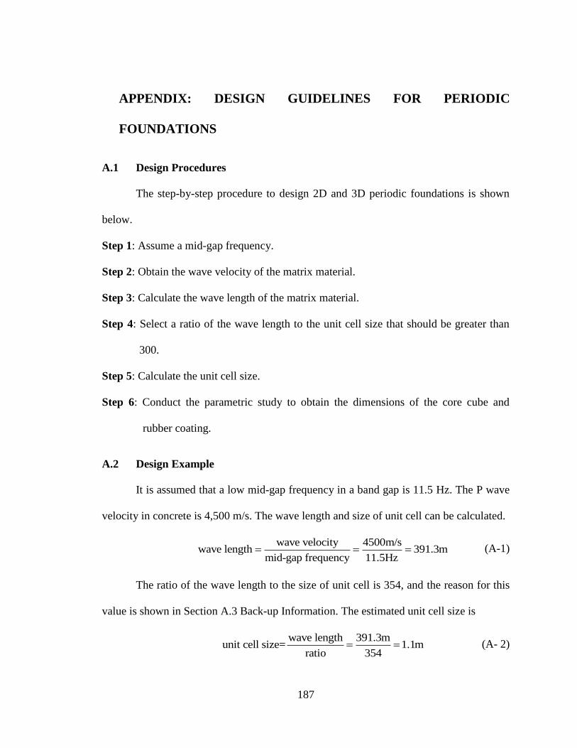
187
A APPENDIX: DESIGN GUIDELINES FOR PERIODIC
FOUNDATIONS
A.1 Design Procedures
The step-by-step procedure to design 2D and 3D periodic foundations is shown
below.
Step 1: Assume a mid-gap frequency.
Step 2: Obtain the wave velocity of the matrix material.
Step 3: Calculate the wave length of the matrix material.
Step 4: Select a ratio of the wave length to the unit cell size that should be greater than
300.
Step 5: Calculate the unit cell size.
Step 6: Conduct the parametric study to obtain the dimensions of the core cube and
rubber coating.
A.2 Design Example
It is assumed that a low mid-gap frequency in a band gap is 11.5 Hz. The P wave
velocity in concrete is 4,500 m/s. The wave length and size of unit cell can be calculated.
wave velocity 4500m/s
wave length 391.3mmid-gap frequency 11.5Hz
(A-1)
The ratio of the wave length to the size of unit cell is 354, and the reason for this
value is shown in Section A.3 Back-up Information. The estimated unit cell size is
wave length 391.3m
unit cell size= 1.1mratio 354
(A- 2)
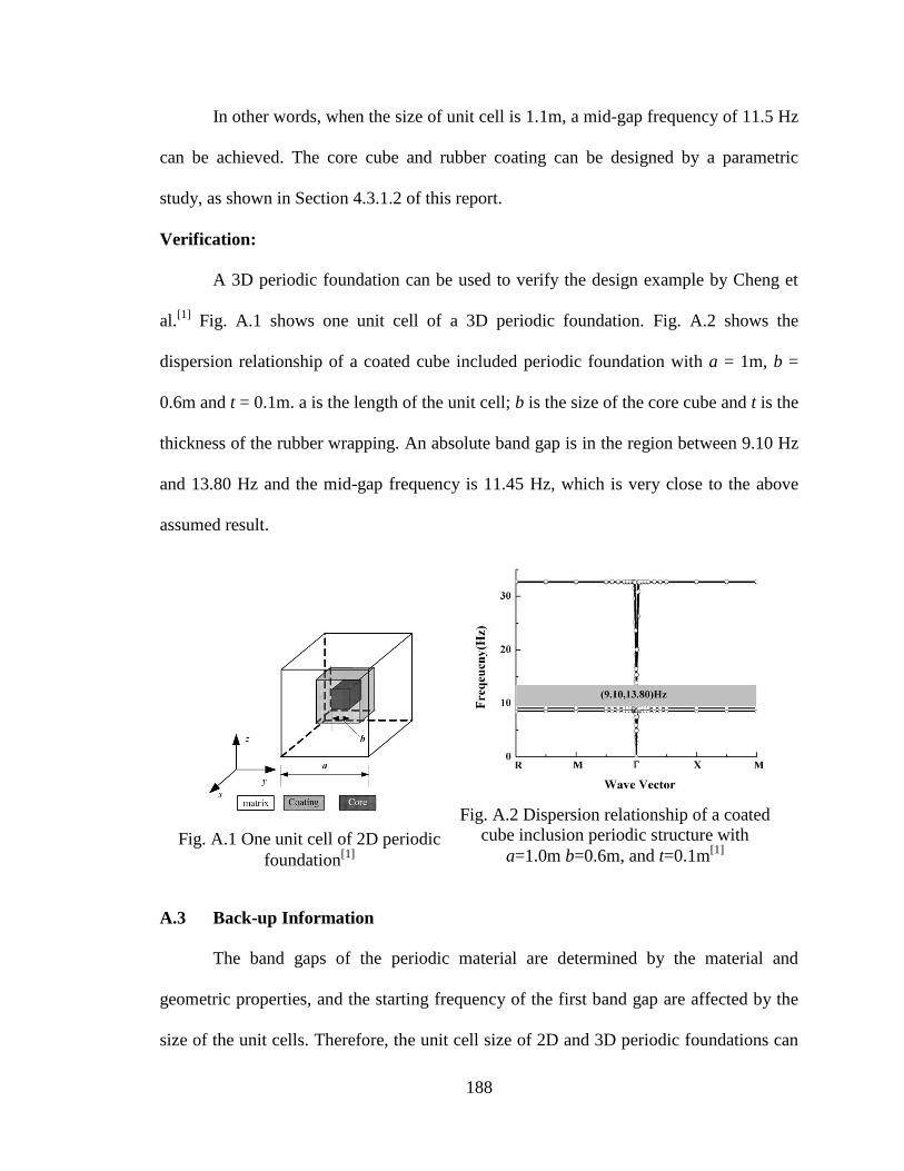
188
In other words, when the size of unit cell is 1.1m, a mid-gap frequency of 11.5 Hz
can be achieved. The core cube and rubber coating can be designed by a parametric
study, as shown in Section 4.3.1.2 of this report.
Verification:
A 3D periodic foundation can be used to verify the design example by Cheng et
al.[1]
Fig. A.1 shows one unit cell of a 3D periodic foundation. Fig. A.2 shows the
dispersion relationship of a coated cube included periodic foundation with a = 1m, b =
0.6m and t = 0.1m. a is the length of the unit cell; b is the size of the core cube and t is the
thickness of the rubber wrapping. An absolute band gap is in the region between 9.10 Hz
and 13.80 Hz and the mid-gap frequency is 11.45 Hz, which is very close to the above
assumed result.
A.3 Back-up Information
The band gaps of the periodic material are determined by the material and
geometric properties, and the starting frequency of the first band gap are affected by the
size of the unit cells. Therefore, the unit cell size of 2D and 3D periodic foundations can
Fig. A.1 One unit cell of 2D periodic
foundation[1]
Fig. A.2 Dispersion relationship of a coated
cube inclusion periodic structure with
a=1.0m b=0.6m, and t=0.1m[1]
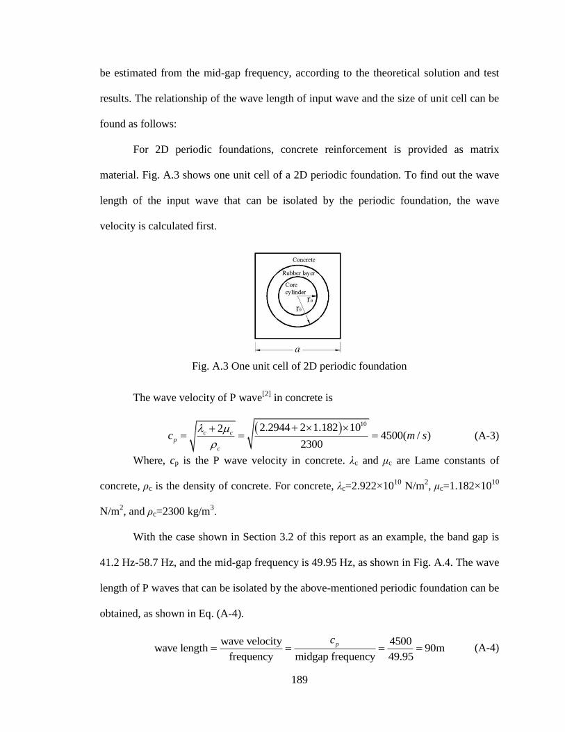
189
be estimated from the mid-gap frequency, according to the theoretical solution and test
results. The relationship of the wave length of input wave and the size of unit cell can be
found as follows:
For 2D periodic foundations, concrete reinforcement is provided as matrix
material. Fig. A.3 shows one unit cell of a 2D periodic foundation. To find out the wave
length of the input wave that can be isolated by the periodic foundation, the wave
velocity is calculated first.
The wave velocity of P wave[2]
in concrete is
102.2944 2 1.182 102
4500( / )2300
c cp
c
c m s
(A-3)
Where, cp is the P wave velocity in concrete. λc and μc are Lame constants of
concrete, ρc is the density of concrete. For concrete, λc=2.922×10¹⁰
N/m2, μc=1.182×10
10
N/m2, and ρc=2300 kg/m
3.
With the case shown in Section 3.2 of this report as an example, the band gap is
41.2 Hz-58.7 Hz, and the mid-gap frequency is 49.95 Hz, as shown in Fig. A.4. The wave
length of P waves that can be isolated by the above-mentioned periodic foundation can be
obtained, as shown in Eq. (A-4).
wave velocity 4500
wave length 90mfrequency midgap frequency 49.95
pc (A-4)
Fig. A.3 One unit cell of 2D periodic foundation
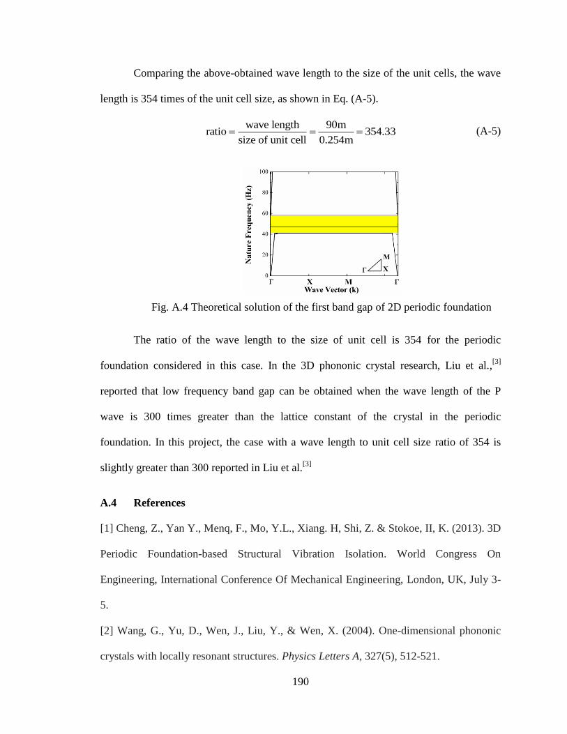
190
Comparing the above-obtained wave length to the size of the unit cells, the wave
length is 354 times of the unit cell size, as shown in Eq. (A-5).
wave length 90m
ratio 354.33size of unit cell 0.254m
(A-5)
The ratio of the wave length to the size of unit cell is 354 for the periodic
foundation considered in this case. In the 3D phononic crystal research, Liu et al.,[3]
reported that low frequency band gap can be obtained when the wave length of the P
wave is 300 times greater than the lattice constant of the crystal in the periodic
foundation. In this project, the case with a wave length to unit cell size ratio of 354 is
slightly greater than 300 reported in Liu et al.[3]
A.4 References
[1] Cheng, Z., Yan Y., Menq, F., Mo, Y.L., Xiang. H, Shi, Z. & Stokoe, II, K. (2013). 3D
Periodic Foundation-based Structural Vibration Isolation. World Congress On
Engineering, International Conference Of Mechanical Engineering, London, UK, July 3-
5.
[2] Wang, G., Yu, D., Wen, J., Liu, Y., & Wen, X. (2004). One-dimensional phononic
crystals with locally resonant structures. Physics Letters A, 327(5), 512-521.
Fig. A.4 Theoretical solution of the first band gap of 2D periodic foundation

191
[3] Liu, Z., Zhang, X., Mao, Y., Zhu, Y. Y., Yang, Z., Chan, C. T., & Sheng, P. (2000).
Locally resonant sonic materials. Science, 289(5485), 1734-1736.

![SEISMIC ROOF ISOLATION OF HALKAPINAR … · most efficient seismic isolation solution for the Halkapınar Gymnasium. In this thesis, theory of seismic isolation, ... [18] (From AASHTO](https://img.pdfslide.us/doc/110x75/5b5ba6ce7f8b9a905c8e7903/seismic-roof-isolation-of-halkapinar-most-efficient-seismic-isolation-solution.jpg)