Development of sectoral indicators for determining

Development of sectoral indicators for determining potential decarbonization opportunity A joint study by IEEJ and Ecofys

– FINAL REPORT –

IEEJ : March 2015. All Rights Reserved.

ECOFYS Germany GmbH | Am Wassermann 36 | 50829 Cologne | T +49 (0)221 27070-100 | F +49 (0)221 27070-011 | E [email protected] | I www.ecofys.com

IEEJ | 13-1, Kachidoki 1-chome, Chuo-ku | 104-0054 Tokyo | T +81 (3)5547 0231 | F +81 (3)5547 0227 | I eneken.ieej.or.jp

Development of sectoral indicators for determining potential decarbonization opportunity A joint study by IEEJ and Ecofys

FINAL REPORT

By:

Ecofys – Markus Hagemann, Ulf Weddige, Sven Schimschar, Niklas Höhne and Thomas

Boermans

IEEJ – Gan Peck Yean, Miki Yanagi, Junko Ogawa, Shen Zhongyuan, Koichi Sasaki, Tohru

Shimizu, Yasushi Ninomiya and Takahiko Tagami

Date: 23 March 2015

© Ecofys and Institute of Energy Economics, Japan 2015




Table of contents

1 Introduction 1

2 Chemical and petrochemical industry 2

2.1 Method 2

2.1.1 Data requirements and data sources 2

2.1.2 Energy consumption per tonne product 3

2.1.3 Energy efficiency index 3

2.1.4 CO2 emissions index 5

2.2 Results 6

2.2.1 EEI 6

2.2.2 CO2 Index 8

2.3 Discussion 8

References 12

3 Pulp and paper industry 13

3.1 Method 13

3.1.1 Data requirements and data sources 13

3.1.2 SEC and BAT 14

3.1.3 Energy efficiency index 15

3.1.4 CO2 emissions index 16

3.2 Results 18

3.2.1 EEI 18

3.2.2 CO2 index 18

3.3 Discussion 20

References 23

4 Steel 24

4.1 Method 24

4.1.1 Macro-data approach 26

4.1.2 Micro-data approach 26

4.1.3 Correction for quality of raw materials 27

4.1.4 CO2 emission indicators 27

4.2 Results 28

4.2.1 SEC for BOF steel in 2000 and 2005 28

References 29

Supplementing information: Electric arc furnace (EAF) in steel sector 30

Methodology 30




Methodology [A] 30

Methodology [B] 30

Results 31

References 32

5 Cement 33

5.1 Overview of the cement manufacturing process 33

5.2 Energy and CO2 indicators in the cement manufacturing process 33

5.3 Method 35

5.3.1 Selection of data 35

5.3.2 GNR indicator 36

5.4 Results 38

5.5 Discussion 41

5.6 Glossary 43

References 44

6 Power 45

6.1 Method 45

6.1.1 Energy efficiency of power generation 45

6.1.2 CO2 intensity of power generation 46

6.2 Results 47

6.2.1 Average efficiency of power generation 47

6.2.2 CO2 intensity of power generation 49

References 52

7 Transport 53

7.1 Method 53

7.1.1 Data sources 53

7.1.2 Average Fuel Efficiency 54

7.2 Results 55

7.2.1 Fuel efficiency comparison for passenger vehicles (2005, 2008) 55

7.2.2 Fuel efficiency comparison for passenger vehicles (2010, 2011) 55

References 57

8 Buildings – heating, cooling and hot water 58

8.1 Method 58

8.1.1 Building stock size 58

8.1.2 Total energy consumption 59

8.1.3 Total emissions 59




8.1.4 Separation by space heating, hot water and space cooling 60

8.1.5 Defining BAU and BAT technologies 61

8.1.6 Formulas 63

8.2 Results 64

8.2.1 Building stock characteristics 64

8.2.2 Energy consumption / emissions (all energy uses) of the building stock 65

8.2.3 Space heating energy consumption and related emissions 66

8.2.4 Hot water energy consumption and related emissions 70

8.2.5 Space cooling energy consumption and related emissions 74

8.3 Conclusions and discussion 77

References 79

Figures

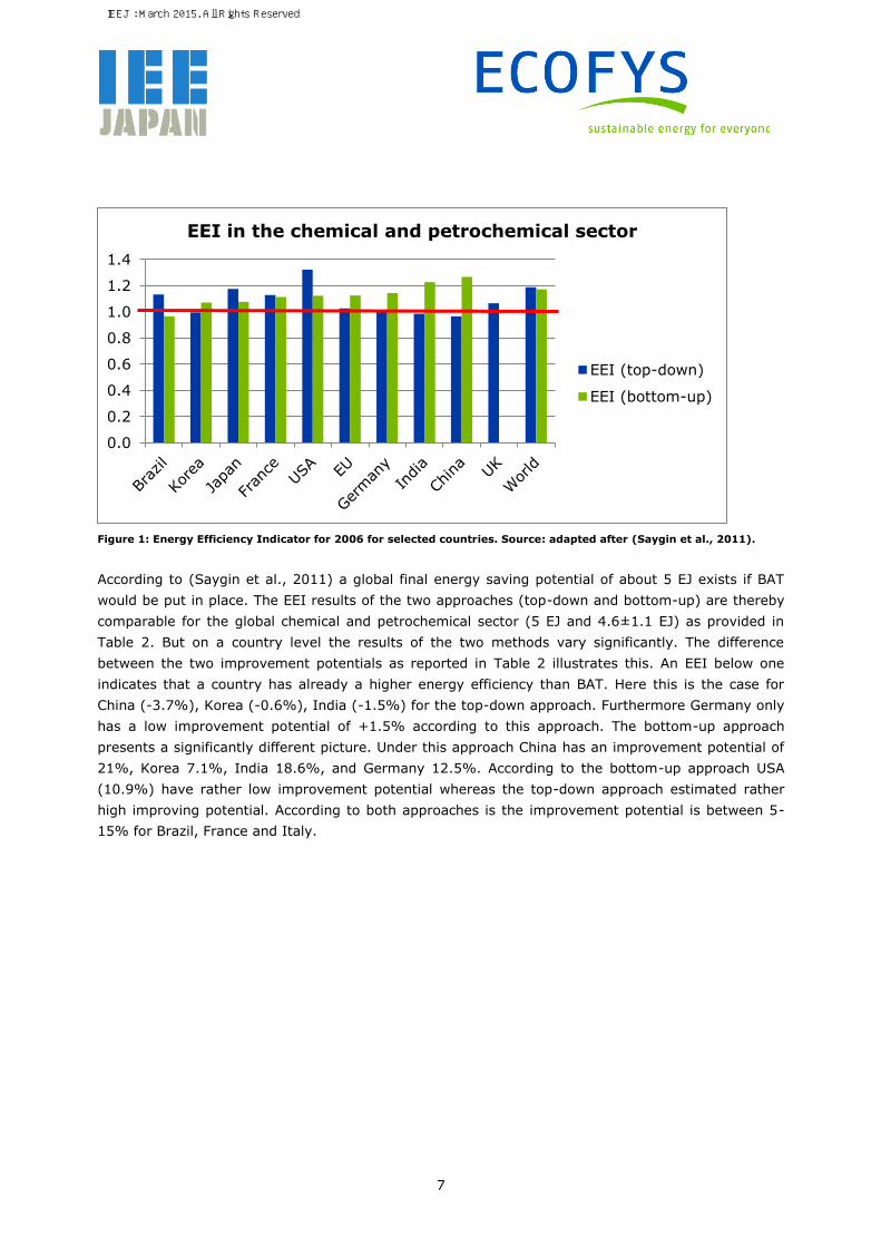
Figure 1: Energy Efficiency Indicator for 2006 for selected countries. Source: adapted after (Saygin et

al., 2011). 7

Figure 2: Current direct CO2 Index (based on the BAT results from the bottom-up approach)

calculated for fuel use scenarios, 2006. Source (Saygin et al., 2009). 8

Figure 3: Specific energy consumption (SEC) and the specific energy use by applying best available

technologies (BAT) in the pulp and paper sector for selected countries in 2011. 14

Figure 4: EEI in the pulp and paper sector of selected countries. 18

Figure 5: CO2 index for the pulp and paper sector for selected countries assuming mainly a switch to

natural gas. 19

Figure 6: CO2 index for the pulp and paper sector for selected countries assuming a fuel split as

currently in Brazil (best practice). 19

Figure 7: Share of worldwide crude steel production by process (2012) (World Steel Association,

2014). 24

Figure 8: Assumed system boundary for iron and steel sector used in Oda et al. (ibid.). 25

Figure 9: Final estimates of SEC for BOF steel in 2000 and 2005 (Oda et al, 2012). 28

Figure 10: Weighted average thermal energy consumption including energy for drying fuels and raw

materials (MJ / tonne clinker) 2012 (WBCSD GNR database). 38

Figure 11: Weighted average net CO2 emission per tonne cement equivalent (excluding CO2 from on-

site power generation) 2012 (kg CO2 / tonne cement equivalent) (WBCSD GNR database). 39

Figure 12: Weighted average power consumption for cement manufacturing per tonne of cement

(kWh/t-cement) 2012 (WBCSD GNR database). 40

Figure 13: Average efficiency of fossil-fired power generation (2012) (compiled from IEA data). 47

Figure 14: Efficiency of coal-fired power generation (2012) (compiled from IEA data). 48

Figure 15: Efficiency of gas-fired power generation (2012) (compiled from IEA data). 49

Figure 16: CO2 intensity for fossil fuel-fired power generation (2012) (compiled from IEA data). 50




Figure 17: CO2 intensity for coal-fired power generation (2012) (compiled from IEA data). 50

Figure 18: CO2 intensity for gas-fired power generation (2012) (compiled from IEA data). 51

Figure 19: Fuel Efficiency Comparison for Passenger Vehicles (LDV) from 2005 to 2011 (GFEI, 2013).

56

Figure 20: Qualitative illustration of correlation between GDP per capita and available floor space per

capita. 58

Figure 21: Scenario comparison for space heating energy consumption. 69

Figure 22: Resulting relative decreases and increases in space heating energy consumption in the

covered countries. 69

Figure 23: Scenario comparison for hot water energy consumption. 72

Figure 24: Resulting relative decreases and increases in hot water energy consumption in the covered

countries. 73

Figure 25: Scenario comparison for space cooling energy consumption. 75

Figure 26: Resulting relative decreases and increases in space cooling energy consumption in the

covered countries. 76




Tables

Table 1: Estimates for the average current SEC for the production of the key chemicals, 2006

(without electricity and excluding feedstock use; data in final energy terms, GJ/tonne of output)

(Saygin et al., 2011). 3

Table 2: Energy efficiency of the chemical and petro chemical sector for 2006 (incl. process energy

and feedstock use, excl. electricity), modified after (Saygin et al., 2011). 6

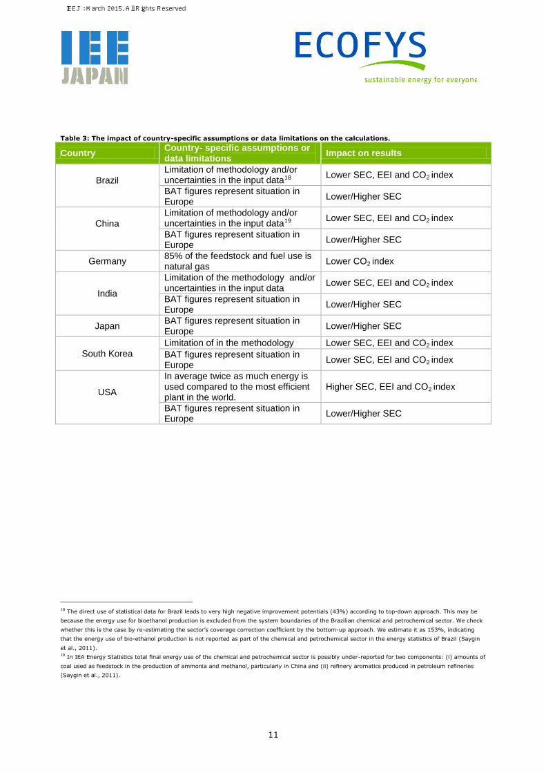
Table 3: The impact of country-specific assumptions or data limitations on the calculations. 11

Table 4: Best practice values for CO2 emissions (Ecofys et al., 2006), (IPCC, 1997). 17

Table 5: The potential impact of country-specific assumptions or data limitations on the calculations.

21

Table 6: Approaches for estimation of BF-BOF SEC (Oda et al. 2012). 25

Table 7: Assumed SEC by route for representative value (Oda et al., 2012). 26

Table 8: Estimated SEC in BF–BOF steel in 2005 based on macro-statistics approach (Oda et al.,

2012). 26

Table 9: Estimated SEC in BF-BOF steel in 2005 based on micro-data approach (Oda et al., 2012). 27

Table 10: Differences between the efficiency indicators suggested and WBCSD-CSI database. 36

Table 11: The share of alternative fuel use in kiln of selected countries (CMA, 2013). 40

Table 12: Data and source. 45

Table 13: Data and source. 46

Table 14: New registrations of LDV covered by fuel economy information by country, 2005 and 2008

(GFEI, 2011). 54

Table 15: Fuel Efficiency Comparison for Passenger Vehicles (2005, 2008) (Unit: Lge/100km) (GFEI,

2011). 55

Table 16: Fuel Efficiency Comparison for Passenger Vehicles (2010, 2011) (GFEI, 2013). 55

Table 17: CO2 emission factors used for the calculation of the emissions in the building sector. 59

Table 18: Considered BAU and BAT technologies, their efficiencies and replacement specifications. 62

Table 19: Assumed energy demands of newly constructed buildings in the BAU and the BAT scenario.

63

Table 20: Building stock size 2012, 2020 and 2030. 64

Table 21: Building stock development 2012-2020. 65

Table 22: Building stock development 2020-2030. 65

Table 23: Total and specific energy consumption and emissions in the building sector of the eight

covered countries in 2012. 66

Table 24: Space heating energy consumption and emissions in the eight covered countries in 2012.66

Table 25: Space heating energy consumption, related emissions and national heating degree days. 67

Table 26: Space heating energy consumption and related CO2 emissions in 2030 - scenario BAU. 67

Table 27: Space heating energy consumption and related emissions in 2030 - scenario BAT. 68

Table 28: Scenario comparison of space heating energy consumption in the covered countries. 70




Table 29: Scenario comparison of space heating related CO2 emissions in the covered countries. 70

Table 30: Hot water energy consumption and emissions in the eight covered countries in 2012. 70

Table 31: Hot water energy consumption and emissions in the eight covered countries in 2012. 71

Table 32: Hot water energy consumption and emissions in the eight covered countries in 2030 -

Scenario BAU. 71

Table 33: Hot water energy consumption and emissions in the eight covered countries in 2030 -

Scenario BAT. 72

Table 34: Scenario comparison of hot water energy consumption in the covered countries. 73

Table 35: Scenario comparison of hot water related CO2 emissions in the covered countries. 73

Table 36: Space cooling energy consumption and emissions in the eight covered countries in 2012. 74

Table 37: Space cooling energy consumption and emissions in the eight covered countries in 2030 -

Scenario BAU. 74

Table 38: Space cooling energy consumption and emissions in the eight covered countries in 2030 -

Scenario BAT. 75

Table 39: Scenario comparison of space cooling energy consumption in the covered countries. 76

Table 40: Scenario comparison of space cooling related CO2 emssions in the covered countries. 76

Table 41: Scenario comparison of space heating, hot water and space cooling energy consumption in

the covered countries. 77

Table 42: Scenario comparison of space heating, hot water and space cooling related CO2-emssions

in the covered countries. 77




Abbreviation

BAT Best available technology

BF-BOF Blast furnace-basic oxygen furnace

CHP Combined heat and power

CHP Combined heat and power plant

CO2 Carbon dioxide

DRI Direct reduced iron

EAF Electric arc furnace

EJ Exajoules

EU European Union

FTP Federal test procedures in the United States

GJ

kWh

LDV

Lge

LHV

MJ

Mt

MWh

NEDC

Nm3-O2

SEC

t

tcs

TFEU

TPEU

Gigajoules

Kilowatt hour

Light-duty vehicle

litre of gasoline equivalent

Lower heating value

Mega joule

Mega tonnes

Megawatt hour

New European driving cycle

normal cubic metres oxygen

Specific energy consumption

Tonnes, for the pulp and paper sector t refers to

air dry tonnes [Adt]

tone crude steel

Total final energy use

Total primary energy use


1

1 Introduction

The international climate negotiations acknowledge that ambition for reducing greenhouse gas

emissions must be increased in the short term in order to keep climate change at safe levels.

The Ad-hoc group on the Durban platform (ADP) in its work stream 1 encouraged countries to submit

national contributions to the global mitigation of greenhouse gas emissions within a 2015

international climate agreement. Under work stream 2 of the ADP countries identify options to

increase ambition to reduce greenhouse gas emissions before 2020. The process aims at identifying

thematic areas where further emission reduction potential is available, where measures have

sustainable development benefits and where global actions have proven to be successful and can be

scaled up.

This report provides a comparative analysis of the energy and carbon intensity indicators across

seven major greenhouse gas emitting sectors namely steel, cement, pulp and paper, chemical, power,

residential and commercial, and transport sectors, of major emitting countries Japan, USA, Russia,

EU, UK, Germany, France, China, India, Indonesia and Brazil. While the analysis does not necessarily

cover all countries mentioned given the lack of adequate and publicly accessible data, it provides

valuable insight into the best practices across nations, and constitutes a benchmark for energy

efficiency improvement and decarbonization.

This report is an output of the project “Development of Sectoral Indicators for Determining Potential

Decarbonization Opportunity” by The Institute of Energy Economics Japan (IEEJ) and Ecofys. It builds

upon an earlier project by IEEJ that aims at quantifying the existing global emission reduction

potential through applying Best Available Technology (BAT).


2

2 Chemical and petrochemical industry

The chemical and petrochemical sector is by far the biggest energy user in the industrial sector, with

about 10% of the global final energy demand and 30%, if feedstock is included. The sector accounts

for around 7% of the global CO2 emissions. The worldwide production is projected to at least double

until 2050. The chemical and petrochemical sector started to improve their energy efficiency,

beginning with the first global oil crisis; back then mainly driven by economical reason due to their

high energy demand and costs. Until today good progress has been made, but still vast improvement

are estimate to exist for this sector, about 10 EJ/y final energy, if applying best available

technologies (BAT), using CHP or improve recycling (OECD/IEA, 2009; Saygin et al., 2011; Fleiter

and Fraunhofer ISI, 2013).

2.1 Method

The chemical and petrochemical sector is a highly multifaceted sector with a large numbers of

processes and multiple-product outcomes. On a global level, it is especially constraint by lacking data

availability for each of these processes and products. Furthermore the definition of the system

boundaries is critical, and countries have often chosen to take different approaches from each other.

For instance some countries include processes / production steps while others exclude these entirely.

In discussions with experts and based on a literature elaboration, we decided to illustrate the energy

efficiency indicator as they are available in literature, rather than re-calculate these complex and

sensitive data sets. Below we therefore describe the approach presented in (Saygin et al., 2011),

who has approached the issue from a bottom up as well as a top-down perspective.

2.1.1 Data requirements and data sources

For the estimation of the Energy efficiency indicator (EEI) and the CO2 indicator the following data

were used:

- Energy consumption data from the IEA Energy Statistics (IEA, 2008a),

- Production data and Specific Energy consumption (SEC) for BAT and the average current

situation (SRI Consulting, 2008).

The production data are based on several data sources, but most chemical processes are retrieved

from (SRI Consulting, 2008). The data was used as reported in (Saygin et al., 2011). Within his

calculations (Saygin et al., 2011) assume that most BAT use natural gas as fuel in the analysed

countries, except for China and India where some BAT are running with coal or oil or in a combination

with natural gas (Saygin et al., 2011). For the calculation of the CO2 index the following datasets

were used:

- fossil-fuel specific emissions factors as reported by the IEA (IEA, 2008b).

- carbon content of the key products were estimated to deduct the stored carbon from the CO2

emissions based on (Saygin et al., 2009).


3

2.1.2 Energy consumption per tonne product

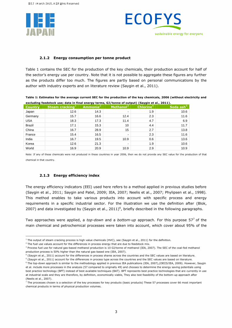
Table 1 contains the SEC for the production of the key chemicals, their production account for half of

the sector’s energy use per country. Note that it is not possible to aggregate these figures any further

as the products differ too much. The figures are partly based on personal communications by the

author with industry experts and on literature review (Saygin et al., 2011).

Table 1: Estimates for the average current SEC for the production of the key chemicals, 2006 (without electricity and

excluding feedstock use; data in final energy terms, GJ/tonne of output) (Saygin et al., 2011).

Country Steam cracking1 Ammonia

2 Methanol

3 Chlorine

4 Soda ash

5

Japan 12.6 14.3 - 1.9 10.6

Germany 15.7 16.6 12.4 2.3 11.6

USA 18.3 17.3 11.4 4.7 6.9

Brazil 17.1 15.3 10 4.4 11.7

China 16.7 28.9 15 2.7 13.8

France 15.4 16.5 - 2.3 11.6

India 16.7 19.5 10.9 0.6 13.6

Korea 12.6 21.3 - 1.9 10.6

World 16.9 20.9 10.9 2.9 10.9

Note: If any of these chemicals were not produced in these countries in year 2006, then we do not provide any SEC value for the production of that

chemical in that country.

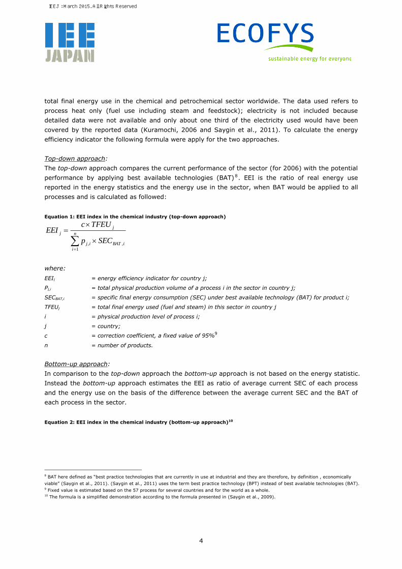
2.1.3 Energy efficiency index

The energy efficiency indicators (EEI) used here refers to a method applied in previous studies before

(Saygin et al., 2011; Saygin and Patel, 2009; IEA, 2007; Neelis et al., 2007; Phylipsen et al., 1998).

This method enables to take various products into account with specific process and energy

requirements in a specific industrial sector. For the illustration we use the definition after (Blok,

2007) and data investigated by (Saygin et al., 2011)6, briefly described in the following paragraphs.

Two approaches were applied, a top-down and a bottom-up approach. For this purpose 577 of the

main chemical and petrochemical processes were taken into account, which cover about 95% of the

1 The output of steam cracking process is high value chemicals (HVC), see (Saygin et al., 2011) for the definition. 2 The fuel use values account for the differences in process energy that are due to feedstock mix. 3 Process fuel use for natural gas-based methanol production is 10 GJ/tonne of methanol (IEA, 2007). The SEC of the coal-fed methanol

production process is 50% higher than the natural gas-based one (IEA, 2007). 4 (Saygin et al., 2011) account for the differences in process shares across the countries and the SEC values are based on literature. 5 (Saygin et al., 2011) account for the differences in process type across the countries and the SEC values are based on literature. 6 The top-down approach is similar to the methodology applied in previous IEA publications (IEA, 2007),(OECD/IEA, 2009). However, Saygin

et al. include more processes in the analysis (57 compared to originally 49) and chooses to determine the energy saving potentials using

best practice technology (BPT) instead of best available techniques (BAT). BPT represents best practice technologies that are currently in use

at industrial scale and they are therefore, by definition, economically viable, They also test feasibility of the bottom-up approach after

(Neelis et al., 2007). 7 The processes chosen is a selection of the key processes for key products (basic products) These 57 processes cover 66 most important

chemical products in terms of physical production volumes.


4

total final energy use in the chemical and petrochemical sector worldwide. The data used refers to

process heat only (fuel use including steam and feedstock); electricity is not included because

detailed data were not available and only about one third of the electricity used would have been

covered by the reported data (Kuramochi, 2006 and Saygin et al., 2011). To calculate the energy

efficiency indicator the following formula were apply for the two approaches.

Top-down approach:

The top-down approach compares the current performance of the sector (for 2006) with the potential

performance by applying best available technologies (BAT) 8. EEI is the ratio of real energy use

reported in the energy statistics and the energy use in the sector, when BAT would be applied to all

processes and is calculated as followed:

Equation 1: EEI index in the chemical industry (top-down approach)

n

i

iBATij

j

j

SECp

TFEUcEEI

1

,,

where:

EEIj = energy efficiency indicator for country j;

Pj,i = total physical production volume of a process i in the sector in country j;

SECBAT,i = specific final energy consumption (SEC) under best available technology (BAT) for product i;

TFEUj = total final energy used (fuel and steam) in this sector in country j

i = physical production level of process i;

j = country;

c = correction coefficient, a fixed value of 95%9

n = number of products.

Bottom-up approach:

In comparison to the top-down approach the bottom-up approach is not based on the energy statistic.

Instead the bottom-up approach estimates the EEI as ratio of average current SEC of each process

and the energy use on the basis of the difference between the average current SEC and the BAT of

each process in the sector.

Equation 2: EEI index in the chemical industry (bottom-up approach)10

8 BAT here defined as “best practice technologies that are currently in use at industrial and they are therefore, by definition , economically

viable” (Saygin et al., 2011). (Saygin et al., 2011) uses the term best practice technology (BPT) instead of best available technologies (BAT). 9 Fixed value is estimated based on the 57 process for several countries and for the world as a whole. 10 The formula is a simplified demonstration according to the formula presented in (Saygin et al., 2009).


5

n

i

ijiBAT

n

i

ijij

j

pSEC

pSEC

EEI

1

,,

1

,,

where:


Pj,i = total physical production volume of a process i in the sector in country j;

SECj,i = the average current specific energy consumption (SEC) for product i.

2.1.4 CO2 emissions index

The CO2 emission index builds on the energy efficiency indicator, more particularly the bottom-up

approach chosen. The CO2 index only takes into account direct CO2 emissions by application of BAT.

Electricity use by sector, the related emissions (indirect emissions), emissions in the use phase and

the waste treatment are not included. To calculate the CO2 index the potential direct CO2 emissions

were estimated by multiplying the actual fossil fuel energy use and feedstock with the specific

emission factor. The carbon captured in the different products is estimated by multiplying their

production volume with the carbon content. This carbon storage is subtracted from the actual direct

CO2 emissions from the sector. This estimated for the current production and for the production using

BAT. By comparison with the results the reduction potentials for direct CO2 emissions can be

estimated (Saygin et al., 2009)11.

Equation 3: CO2 index in the chemical industry

)()(

)()(

,,

1

,,

1

,,,,

2

ijij

n

i

ijBAT

n

i

ijijijSEC

j

pvCeF

pvCeF

IndexCO

where:

FBAT = fossil fuel and feedstock used for product i by applying BAT in country j;

FSEC = fossil fuel and feedstock used for product i by applying SEC in country j;

e = fossil fuel specific CO2 emissions factors;

C = carbon capture in product i in county j;

pv = production volume of product i in country j;

j = country;

i = produced product;


11 For the CO2 index we inverse the calculation and switch nominator and numerator defined by (Höhne et al., 2006).


6

2.2 Results

2.2.1 EEI

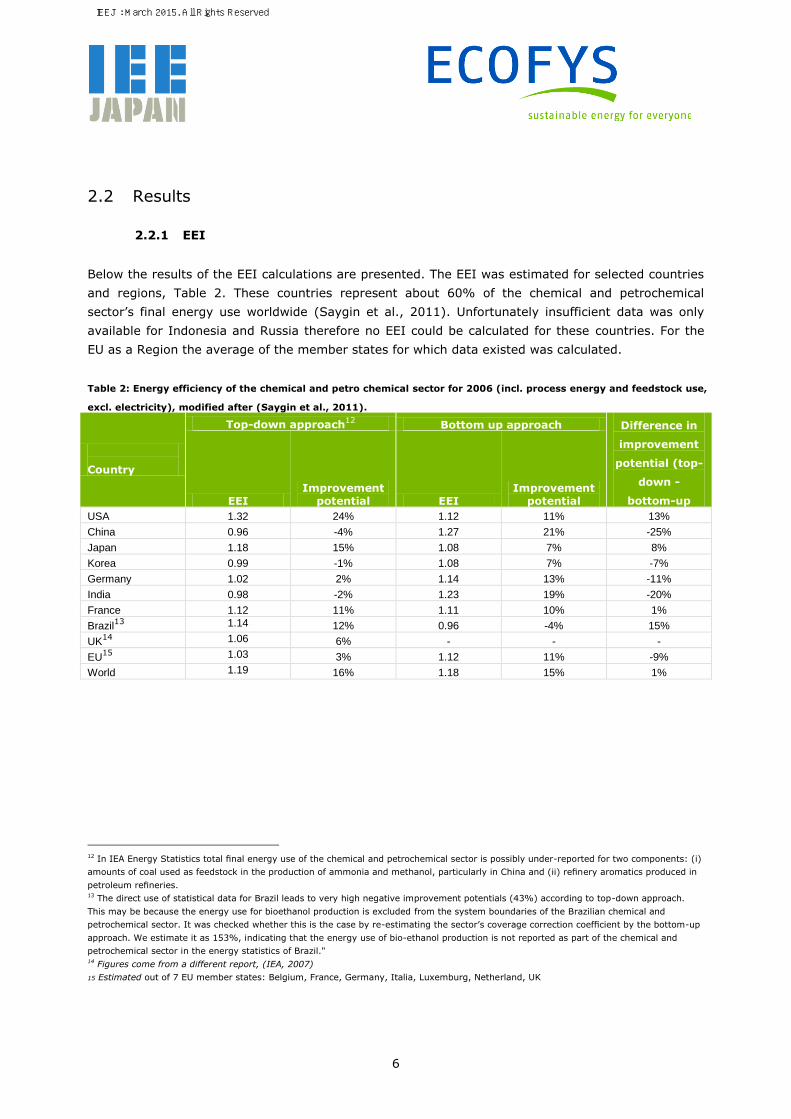
Below the results of the EEI calculations are presented. The EEI was estimated for selected countries

and regions, Table 2. These countries represent about 60% of the chemical and petrochemical

sector’s final energy use worldwide (Saygin et al., 2011). Unfortunately insufficient data was only

available for Indonesia and Russia therefore no EEI could be calculated for these countries. For the

EU as a Region the average of the member states for which data existed was calculated.

Table 2: Energy efficiency of the chemical and petro chemical sector for 2006 (incl. process energy and feedstock use,

excl. electricity), modified after (Saygin et al., 2011).

Country

Top-down approach12

Bottom up approach Difference in

improvement

potential (top-

down -

bottom-up EEI Improvement

potential EEI Improvement

potential

USA 1.32 24% 1.12 11% 13%

China 0.96 -4% 1.27 21% -25%

Japan 1.18 15% 1.08 7% 8%

Korea 0.99 -1% 1.08 7% -7%

Germany 1.02 2% 1.14 13% -11%

India 0.98 -2% 1.23 19% -20%

France 1.12 11% 1.11 10% 1%

Brazil13

1.14 12% 0.96 -4% 15%

UK14

1.06 6% - - -

EU15

1.03 3% 1.12 11% -9%

World 1.19 16% 1.18 15% 1%

12 In IEA Energy Statistics total final energy use of the chemical and petrochemical sector is possibly under-reported for two components: (i)

amounts of coal used as feedstock in the production of ammonia and methanol, particularly in China and (ii) refinery aromatics produced in

petroleum refineries. 13 The direct use of statistical data for Brazil leads to very high negative improvement potentials (43%) according to top-down approach.

This may be because the energy use for bioethanol production is excluded from the system boundaries of the Brazilian chemical and

petrochemical sector. It was checked whether this is the case by re-estimating the sector’s coverage correction coefficient by the bottom-up

approach. We estimate it as 153%, indicating that the energy use of bio-ethanol production is not reported as part of the chemical and

petrochemical sector in the energy statistics of Brazil." 14 Figures come from a different report, (IEA, 2007)

15 Estimated out of 7 EU member states: Belgium, France, Germany, Italia, Luxemburg, Netherland, UK


7

Figure 1: Energy Efficiency Indicator for 2006 for selected countries. Source: adapted after (Saygin et al., 2011).

According to (Saygin et al., 2011) a global final energy saving potential of about 5 EJ exists if BAT

would be put in place. The EEI results of the two approaches (top-down and bottom-up) are thereby

comparable for the global chemical and petrochemical sector (5 EJ and 4.6±1.1 EJ) as provided in

Table 2. But on a country level the results of the two methods vary significantly. The difference

between the two improvement potentials as reported in Table 2 illustrates this. An EEI below one

indicates that a country has already a higher energy efficiency than BAT. Here this is the case for

China (-3.7%), Korea (-0.6%), India (-1.5%) for the top-down approach. Furthermore Germany only

has a low improvement potential of +1.5% according to this approach. The bottom-up approach

presents a significantly different picture. Under this approach China has an improvement potential of

21%, Korea 7.1%, India 18.6%, and Germany 12.5%. According to the bottom-up approach USA

(10.9%) have rather low improvement potential whereas the top-down approach estimated rather

high improving potential. According to both approaches is the improvement potential is between 5-

15% for Brazil, France and Italy.

0.0

0.2

0.4

0.6

0.8

1.0

1.2

1.4

EEI in the chemical and petrochemical sector

EEI (top-down)

EEI (bottom-up)


8

2.2.2 CO2 Index

Figure 2: Current direct CO2 Index (based on the BAT results from the bottom-up approach) calculated for fuel use

scenarios, 2006. Source (Saygin et al., 2009).16

*This CO2 index is calculated assuming that the current and future breakdown of fuel use and feedstock mix of the chemical and petrochemical sector of

the selected countries are identical.

The CO2 emissions index is presented in Figure 2 for the bottom-up approach. Two different figures

are reported for each country, the first assuming the fuel mix as reported in 2006 and the second

assuming a fuel switch to natural gas. Note that the CO2 index is calculated assuming that the current

and future breakdown by fuel use and the feedstock mix of the chemical and petrochemical sector for

the selected countries are identical. The emission reduction potential is in the order of 20-35% with

current fuel use and feedstock mix and about 25%-60% if a switch to natural gas would be

considered (Saygin et al., 2009).

2.3 Discussion

Energy efficiency index:

The top-down approach overestimates the energy saving potential for some of the countries such as

Japan, but mainly underestimates it for other such as Korea, China, or India. For these countries the

EEI was below 1, indicating a potential beyond the BAT. This indicates the limitations of a top-down

16 The extreme high figure in the switch to gas scenario for China can be explained by the switch from the carbon-intensive coal in China to

less carbon-intensive natural gas (see also 2.1.1). There is not such a high change in other countries, because total energy use is a mix of

coal, oil and natural gas whereas in China, it is mainly coal.

0.0

0.5

1.0

1.5

2.0

2.5

3.0

3.5

4.0

4.5

5.0

CO2 index in the chemical and petrochemical sector

Current fuel mix*

(bottom-up)

Switch to natural gas

(bottom-up)

14.3


9

approach and highlights the benefits of using country specific data sources as done in the bottom up

approach17. Reasons for this are after (Saygin et al., 2011):

Complexity of the chemical and petrochemical sector; multi-products processes and complex

material flows.

Reliable input data like technology data, statistical data (energy, production data) reported by

the different countries, which significant influence the outcome of the EEI.

Missing out appropriate integration of heat cascading for the BAT and the SEC, thus the

comparison calculated process heat and energy statistics not in totally line.

BAT and many SEC estimation are based on European data sets and uniformed for whole

world, since country specific or worldwide data were not available.

Uncertainties fuzzy delimitation in accounting the energy statistic between chemical and

petrochemical and the refinery sector.

Estimation of one worldwide coverage correction coefficient (95%), which fits for global

average estimations, but not for each country separately.

The top-down approach provides good insights energy efficiency ranges, but should be handled with

care since it is not robust enough to give definite insights in country ranking concerning energy

saving potentials. The bottom-up approach is an alternative, but is also limited by the provided input

data.

Table 3 gives a brief overview of impacts on the calculation, due to setting certain assumption or data

limitation.

The reason for the relative low saving potential in the chemical and petrochemical sector (compared

to other sectors like iron and steel 29%, cement industry 23%) is the high share of feedstock use for

which no savings are possible (Saygin et al., 2011). In order to improve this other energy efficiency

improvements beside BAT could be taken into account such as like biomass feedstock use, higher

recycling rates or a more intensive use of CHP.

CO2 index:

There is a gap in the product scope for estimating the carbon storage and accounting for other

uncertainties. For some products carbon storage is credited, but parts of this carbon are released

later on, e.g. as a consequence of waste management activities or in case of urea fertilizer, where

the CO2 emissions are accounted to the agriculture use. CO2 process emissions not related to the use

of fossil fuels are not. They can be a significant share of the industrial CO2 emissions. All the

uncertainties highlighted and limitation on data availability and reliability highlighted for the EEI

above are also valid for the CO2 index.

17 The availability of energy data is limited in the chemical and petrochemical sector. General reasons are: a) bad data quality and only

limited available or accessible; b) the available data often don’t match each other and are difficult to compare (different ascertainment

approaches). The limitation effects both approached, top-down and bottom-up. The outcome has to be handled with care and conclusions

have to be seen within this perspective.


10

Due to these limitations, the index can best be used as an indication of the emissions and reduction

potential. It may not well suited for country specific emission reduction targets setting and neither for

ranking the countries (Saygin et al., 2009).


11

Table 3: The impact of country-specific assumptions or data limitations on the calculations.

Country Country- specific assumptions or data limitations

Impact on results

Brazil

Limitation of methodology and/or uncertainties in the input data18

Lower SEC, EEI and CO2 index

BAT figures represent situation in Europe

Lower/Higher SEC

China

Limitation of methodology and/or uncertainties in the input data19



Lower/Higher SEC

Germany 85% of the feedstock and fuel use is natural gas

Lower CO2 index

India

Limitation of the methodology and/or uncertainties in the input data



Lower/Higher SEC

Japan BAT figures represent situation in Europe

Lower/Higher SEC

South Korea

Limitation of in the methodology Lower SEC, EEI and CO2 index



USA

In average twice as much energy is used compared to the most efficient plant in the world.

Higher SEC, EEI and CO2 index


Lower/Higher SEC

18 The direct use of statistical data for Brazil leads to very high negative improvement potentials (43%) according to top-down approach. This may be

because the energy use for bioethanol production is excluded from the system boundaries of the Brazilian chemical and petrochemical sector. We check

whether this is the case by re-estimating the sector’s coverage correction coefficient by the bottom-up approach. We estimate it as 153%, indicating

that the energy use of bio-ethanol production is not reported as part of the chemical and petrochemical sector in the energy statistics of Brazil (Saygin

et al., 2011). 19 In IEA Energy Statistics total final energy use of the chemical and petrochemical sector is possibly under-reported for two components: (i) amounts of

coal used as feedstock in the production of ammonia and methanol, particularly in China and (ii) refinery aromatics produced in petroleum refineries

(Saygin et al., 2011).


12

References

Blok, K., 2007. Introduction to Energy Analysis. Techne Press, Amsterdam.

Fleiter, T., Fraunhofer ISI, 2013. Energieverbrauch und CO2-Emissionen industrieller

Prozesstechnologien: Einsparpotenziale, Hemmnisse und Instrumente. Fraunhofer-Verl.,

Stuttgart.

Höhne, N., Moltmann, S., Lahme, E., Worrell, E., Graus, W., 2006. CO2 emission reduction potential

under a sectoral approach post 2012. Köln.

IEA, 2008a. Energy balances for OECD and non-OECD countries - 2008. International Energy Agency,

Paris, France.

IEA, 2008b. CO2 Emissions from Fuel Combustion 2008. Organisation for Economic Co-operation and

Development, Paris.

IEA, 2007. Tracking Industrial Energy Efficiency and CO2 Emissions. Paris, France.

Kuramochi, T., 2006. Differentiation of greenhouse gas emissions reduction commitments based on a

bottom-up approach: Focus on industrial energy efficiency benchmarking and future industrial

activity indicators. Utrecht University Department of Science, Technology and Society.

Neelis, M., Patel, M., Blok, K., Haije, W., Bach, P., 2007. Approximation of theoretical energy-saving

potentials for the petrochemical industry using energy balances for 68 key processes. Energy

32, 1104–1123. doi:10.1016/j.energy.2006.08.005

OECD/IEA, 2009. Energy Technology Transitions for Industry: Strategies for the Next Industrial

Revolution. International Energy Agency (IEA), Paris, France.

Phylipsen, G.J.M., Blok, K., Worrell, E., 1998. Handbook on International Comparisons of Energy

Efficiency in the Manufacturing Industry. Department of Science, Technology and Society,

Utrecht University.

Saygin, D., Patel, D.M.K., 2009. Material and Energy Flows in the chemical sector in Germany.

Saygin, D., Patel, M.K., Tam, C., Gielen, D.J., 2009. Chemical and Petrochemical Sector - Potential of

best practice technology and other measures for improving energy efficiency. International

Energy Agency (IEA), Paris, France.

Saygin, D., Patel, M.K., Worrell, E., Tam, C., Gielen, D.J., 2011. Potential of best practice technology

to improve energy efficiency in the global chemical and petrochemical sector. Energy 36,

5779–5790. doi:10.1016/j.energy.2011.05.019

SRI Consulting, 2008. Production, capacity and capacity average age data for selected chemical and

for selected countries and for OECD regions.


13

3 Pulp and paper industry

In the pulp and paper industry a range of products are produced, ranging from low quality paper for

wrapping and packaging to high quality printing paper. Each product has specific process and energy

requirements that can vary largely. The pulp and paper industry processes fibrous raw material or

recycling paper into paper. This includes several processes like raw materials preparation, pulping

(chemical, semi-chemical, mechanical, or waste paper), bleaching, chemical recovery, pulp drying,

and papermaking. The most energy consuming processes are pulping and drying (Worrell et al.,

2008). The energy consumption of the pulp and paper processes in generally depends on the quality

of the paper class to be produced. The large differences in the pulp characteristics and paper grades

influence the energy consumption of the technologies used, i.e. also those of the best available

technologies. The differences make it difficult to represent the whole range, because energy use

depend on various specific properties like the raw material used, the grade and quality of the product

or level of cascade energy use (Worrell et al., 2008). On a global level the IEA estimates potential

savings by adopting BAT at approximately 1.4 EJ/year and 80Mt CO2/year for the pulp and paper

sector (OECD/IEA, 2009).

In comparison to the chemical industry the EEI had to be calculated separately as no up- to date

study exists. We have therefore modified the approach already used in (Höhne et al., 2006, Phylipsen

et al., 1998) and applied it here. In comparison to the approach described there, our calculations

here assume however only one BAT value for the entire pulp and paper making process per paper

product (see also below for a description of how this was implemented).

3.1 Method

3.1.1 Data requirements and data sources

For the estimation of the Energy efficiency indicator (EEI) and the CO2 indicator the following data

sets were used:

- Energy consumption per country, for the entire pulp and paper industry from the IEA Energy

Statistics (IEA, 2013),

- Production data for both pulp and paper production per country and by different processes

types from FAO (FAO, 2013)

- Specific energy consumption (SEC) for BAT for both integrated (i.e. one BAT value for the

entire pulp and paper process) and separate (i.e. BAT values for each step, pulp and paper,

separately) from Worrell et al., 2008.

For the estimation of the CO2 index the following additional data sources were used:

- fossil fuel specific emissions factors from the IEA (IEA, 2012).


14

3.1.2 SEC and BAT

Below the current SEC per country as well as the achievable SEC per country based on BAT are

depicted. The country specific energy consumption figures are derived from IEA energy statistics (IEA,

2013).

The BAT numbers are derived using the following approach: We assume for BAT20 that the steam and

electricity are generated in a cogeneration (CHP) installation and that 70% of the produced paper is

made from recycled material21. The latter assumption is based on an expert judgement; in reality the

maximum achievable recycling rate for the different paper types can vary largely. Furthermore we

assume that the pulp and the papermaking process are performed on the same factory site, since the

integrated approach is the most energy efficient approach22. The reason for this are the possibilities

to supply heat energy, a smaller need for drying the pulp and minimized transportation (see also

Equation 4) (Worrell et al., 2008).

Figure 3: Specific energy consumption (SEC) and the specific energy use by applying best available technologies

(BAT) in the pulp and paper sector for selected countries in 2011.

20 International BAT energy use in pulp and papermaking technology is based on wood-based fibres. Hence, the identified best practice

technologies may not be applicable to non-wood fibre based pulp mills. Even though there is increased interest in the use of non-wood fibres

internationally, only a few best practice technologies are available (Worrell et al., 2008).

It is uncommon the SEC is lower than the BAT as is it presented here. The presented BAT values are the most up to date values available.

Reason for that can be multifaceted, mainly due to insufficient data quality. 21 The 70% recycling rate is based on expert’s opinion and experiences in practice. Some pioneer’s country like Korea or Germany already

achieved 80-90%. We think the recycling rates can be higher, even though a 100% (global level) will not be reached due locked products or

product losses during life cycle. Future-wise we don’t see a technical limitation to make paper from recycling paper, even though today the

literature quotes that some types/quality of paper can only be produced with wood-pulp. 22 Currently the pulp- and the paper-making process are mainly separated geographically speaking.

0

5

10

15

20

25

GJ/

t

Pulp & paper

SEC (2011)

BAT


15

3.1.3 Energy efficiency index

The EEI was calculated using a similar approach as the top-down approach described in chapter

2.1.323. The calculation takes into account that different products have different energy needs24. For

each product we defined a specific BAT energy consumption based on literature values from 25

(Worrell et al., 2008). We then calculated the BAT energy use per country by multiplying the BAT

SEC by the country specific production per product. Finally, we divided the total final energy used by

the sum of BAT values for the pulp and paper sector in that country.

Equation 4: EEI in the pulp and paper industry

n

i

iBATij

j

j

SECp

TFEUEEI

1

,,

where:


Pj,i = total production volume product i in the sector in country j;

TFEUj = total final energy used in this sector26

in country j

SECBAT,i = specific final energy consumption (SEC) under best available technology (BAT) for product i;

i = physical production level of process i;

j = country;


A country using BAT would have an energy efficiency index of 1. An index of 1.2 would indicate that

that country uses 20% more energy than BAT.

We use the final energy consumption when calculating the EEI, to show the energy efficiency of that

sector excluding the efficiency of the electricity production. This gives the possibility to compare the

energy efficiency of the pulp and paper sector in different countries with each other, while excluding

the indirect influence from power generation efficiency. This gives a clear picture of the actual energy

efficiency of the sector and is a measure for energy efficiency improvement opportunities.

Many countries import pulp to cover their paper production (e.g. China, EU), others produce more

pulp than they need for their paper production and export them (Brazil, US, Indonesia). This

influences the EEI, since the calculations are based on the paper production only. The BAT figures

23 Please note that even though the bottom-up approach might be more accurate as shown for the chemical sector, we do not have the data

necessary to replicate this approach for the paper industry 24 The calculations differentiate between papers types like news prints, sanitary paper, wrapping paper, paper board etc. But do not

differentiate between quality grades of the each paper types, e.g. different writing papers. Mainly due to missing data availability. 25 BAT values were estimated for final energy use. 26 The Pulp and paper sector include energy consumption of the printing and publication sector as well given in the IEA energy data (IEA,

2013).


16

assume an integrated approach, where pulp and paper is produced on the same site. With import of

pulp the energy consumption for the production of the pulp is accounted for by the energy statistics

of the exporting country. The opposite is the case for exporting countries. Therefore we introduced a

penalty for importing countries and a credit for exporting countries in the calculations27.

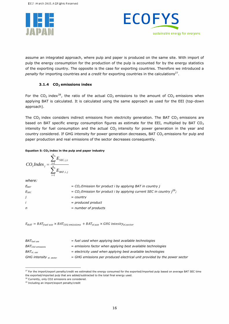
3.1.4 CO2 emissions index

For the CO2 index28, the ratio of the actual CO2 emissions to the amount of CO2 emissions when

applying BAT is calculated. It is calculated using the same approach as used for the EEI (top-down

approach).

The CO2 index considers indirect emissions from electricity generation. The BAT CO2 emissions are

based on BAT specific energy consumption figures as estimate for the EEI, multiplied by BAT CO2

intensity for fuel consumption and the actual CO2 intensity for power generation in the year and

country considered. If GHG intensity for power generation decreases, BAT CO2 emissions for pulp and

paper production and real emissions of the sector decreases consequently.

Equation 5: CO2 index in the pulp and paper industry

n

i

jiBAT

n

i

ijSEC

j

E

E

IndexCO

1

,,

1

,,

2

where:

EBAT = CO2 Emission for product i by applying BAT in country j

ESEC = CO2 Emission for product i by applying current SEC in country j29

;

j = country

i = produced product

n = number of products

BATfuel use = fuel used when applying best available technologies

BATCO2 emissions = emissions factor when applying best available technologies

BATel. use = electricity used when applying best available technologies

GHG intensity el. sector = GHG emissions per produced electrical unit provided by the power sector

27 For the import/export penalty/credit we estimated the energy consumed for the exported/imported pulp based on average BAT SEC time

the exported/imported pulp that are added/subtracted to the total final energy used. 28 Currently, only CO2 emissions are considered. 29 Including an import/export penalty/credit


17

Table 4 shows the best practice values for CO2 emissions from fuel combustion for pulp and paper

sector, based on IPCC report (IPCC, 1997) and expert judgement.

Table 4: Best practice values for CO2 emissions (Ecofys et al., 2006), (IPCC, 1997).

Product Best practice CO2 emissions factor for fuel

consumption [kt CO2/PJ fuel] Assumption

Wood Pulp mechanical 56 100% natural gas

chemical 56 100% natural gas

other 56 100% natural gas

Fibre Pulp other 56 100% natural gas

recovered 56 100% natural gas

Paper news print 56 100% natural gas

printing and

writing 50

25% biomass, 25% oil and

50% natural gas

household and

sanitary 50

25% biomass, 25% oil and

50% natural gas

wrapping,

packaging,

board

56 100% natural gas

other and board 56 100% natural gas

Alternatively to the above assumed use of largely natural gas as an energy source by BAT technology,

we have also taken a second approach. Hereby we have determined the current specific emissions

factor for a Brazil, a country that has been able to rely largely on biomass as an energy source.


18

3.2 Results

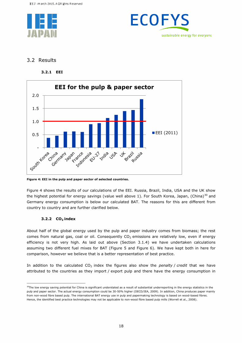
3.2.1 EEI

Figure 4: EEI in the pulp and paper sector of selected countries.

Figure 4 shows the results of our calculations of the EEI. Russia, Brazil, India, USA and the UK show

the highest potential for energy savings (value well above 1). For South Korea, Japan, (China)30 and

Germany energy consumption is below our calculated BAT. The reasons for this are different from

country to country and are further clarified below.

3.2.2 CO2 index

About half of the global energy used by the pulp and paper industry comes from biomass; the rest

comes from natural gas, coal or oil. Consequently CO2 emissions are relatively low, even if energy

efficiency is not very high. As laid out above (Section 3.1.4) we have undertaken calculations

assuming two different fuel mixes for BAT (Figure 5 and Figure 6). We have kept both in here for

comparison, however we believe that is a better representation of best practice.

In addition to the calculated CO2 index the figures also show the penalty / credit that we have

attributed to the countries as they import / export pulp and there have the energy consumption in

30The low energy saving potential for China is significant understated as a result of substantial underreporting in the energy statistics in the

pulp and paper sector. The actual energy consumption could be 30-50% higher (OECD/IEA, 2009). In addition, China produces paper mainly

from non-wood fibre based pulp. The international BAT energy use in pulp and papermaking technology is based on wood-based fibres.

Hence, the identified best practice technologies may not be applicable to non-wood fibre based pulp mills (Worrell et al., 2008).

-

0.5

1.0

1.5

2.0

EEI for the pulp & paper sector

EEI (2011)


19

their country while not using the pulp in the paper process (export) or import the pulp whereby the

energy consumption does not show up in the energy balances of the country and needs to be added.

Figure 5: CO2 index for the pulp and paper sector for selected countries assuming mainly a switch to natural gas.

Figure 6: CO2 index for the pulp and paper sector for selected countries assuming a fuel split as currently in Brazil

(best practice).

0.0

0.2

0.4

0.6

0.8

1.0

1.2

1.4

1.6

CO2 Index in the pulp & paper sector

CO2 index - export

credit (2011)

CO2 index - import

penalty (2011)

CO2 Index (2011)

0.0

0.5

1.0

1.5

2.0

2.5

Chin

a

South

Kore

a

Germ

any

Japan

EU

-27

Fra

nce

USA

Indonesia

Russia

Bra

zil

UK

India

CO2 Index in the pulp & paper sector

CO2 index - export

credit penalty (2011)

CO2 index - import

penalty (2011)

CO2 Index (2011)


20

Comparing the two assumptions, as expected, the CO2 index is a lot higher for a number of countries

if we assume that the fuel mix will mainly rely on natural gas. What can be observed is that some

countries, namely China and South Korea, even under the ambitious scenario still have an EEI below

1. This fact could also be partially explained by the fact that there is a large share of autonomous

production of energy in the sector, using residues from the process as input to produce electricity or

heat. These do not necessarily show up in the energy balances. In Europe for instance, the sector

itself produces about 46 % of the electricity it consumes (EC, 2012).

3.3 Discussion

Below is a summary by country of the most important data constraints / national circumstances that

we have identified and how they influence the calculations above.


21

Table 5: The potential impact of country-specific assumptions or data limitations on the calculations.


Impact on results

Brazil High share of pulp export

Higher SEC and CO2 index or lower SEC31

High share of newer pulping mills Lower SEC, EEI and CO2 index

China

Uncertainties in the reported energy data 32

Lower SEC, EEI, CO2 index Extreme high share of non-wood-fibre pulp mills.

CO2 intensive fuel mix used for electricity in the production

Higher CO2 index

France High share of medium/old pulp mills Higher SEC

Germany

High share of newer pulping mills Lower SEC,EEI, CO2 index

High share of recycled material in the pulp production.

Lower SEC,EEI, CO2 index

Uncertainties in the reported energy data on biomass use33

Higher CO2 Index

India

High share of small and medium pulp and paper plants (IEA, 2011)

Higher SEC, EEI

Pulp production uses a high share of agricultural residues.

Higher SEC, EEI

CO2 intensive fuel mix used for electricity in the production

Higher CO2 Index

Indonesia High share of exported pulp Higher SEC, CO2 index or lower SEC, CO2 index34

Japan High share of recycled material in the pulp production.


South Korea High share of newer pulping mills Lower SEC,EEI, CO2 index

High share of recycled material in the pulp production.


Russia

High share on old pulp and paper mills (OECD/IEA, 2009)

Higher SEC, EEI, CO2 index

High share of CO2 intensive fuel mix used for electricity in the production

High CO2 Index

UK

High share of energy consumption by the publishing and printing subsector embedded into the total pulp and paper sector35.

Higher SEC, EEI and CO2 Index

USA

High share on old pulp and paper mills (OECD/IEA, 2009)

Higher SEC, EEI, CO2 index

31 Without the applied import penalty respectively export credit the SEC would be higher, with the applied import penalty respectively export

credit the SEC could also be underestimated. 32 (Kong, 2014) estimates a SEC from 13.2 GJ/tonne (2010) in national pulp and paper study. Compared to the here 7.4 GJ/tonne (2011). 33 Many countries do not report the biomass energy used under the pulp and paper sector in the international energy statistics, but instead

under other non-specific industries (UNIDO, 2010) 34 Without the applied import penalty respectively export credit the SEC would be higher, with the applied import penalty respectively export

credit the SEC could also be underestimated. 35 UK has big printing sector that influence the IEA energy statistics, actually it is assumed that 30-50% of the reported total energy

consumption in pulp and paper (and printing) sector is used by the printing and publishing sub-sector (Kuramochi, 2006).


22


Impact on results

High share of exported pulp Higher SEC, CO2 index or lower SEC, CO2 index

High share of CO2 intensive fuel mix used for electricity in the production electricity in the production

Higher CO2 Index

High share of energy consumption by the publishing and printing subsector embedded into the total pulp and paper sector

Higher SEC, EEI and CO2 Index

There are a number of limitations with the data used:

The IEA data on energy consumption for the pulp and paper sector also include the energy

consumption of the printing and publishing sub-sector. E.g. in the Netherland about 15% of

the energy consumption can be accounted for the printing and publishing sector (Worrell et

al., 1994) we aspect them even higher for UK and US, among other due to their large English

print market. This could not be distinctive in our approach. This can have a big influence on

the SEC and EEI, depending on the share of energy consumption from the printing and

publishing sector on the total pulp, paper and printing sector reported by the IEA statistics.

So probably less energy is consumed by the pulp and paper sector as assumes in our data.

High share of CHP makes it difficult to estimate reliable energy consumption data (Fleiter and

Fraunhofer ISI, 2013). The integrated nature of processes in the pulp and paper sector make

it difficult to account reliably for the sector's energy demand. For instance, only parts of the

biomass energy used is reported under the pulp and paper sector in IEA data, but instead

under other non-specific industries (OECD/IEA, 2009). This all effects EEI and CO2 index.

“The United Nations Food and Agricultural Organization (FAO) provides comprehensive

statistics on pulp and paper production, but categories for different paper grades do not

match what is required for a more detailed indexed comparison of energy use by different

paper grades. These indicators are not intended for benchmarking, which should be done on

an individual mill or machine level” (IEA, 2007).

Integrated pulp and paper mills result in energy savings due to the reduced need to e.g. dry

pulp and offers opportunities to provide a better heat integration (Worrell et al., 2008). To

implement this integration approach on global market level might be difficult, especially if

considering the large amounts of pulp that are imported/ exported.

It is uncommon that the SEC is lower than the BAT. The presented SEC and BAT values are

the most up to date values available. Reason for that can be multifaceted as mentioned

above, but most probably due to data limitations.

In general, the outcome should be handled with care. Conclusions should be seen within the

perspective of the limitation of data availability and method applied.


23

References

EC, 2012. Technology Information Sheet - Energy Efficiency and CO2 Reduction in the Pulp and Paper

Industry.

Ecofys et al., 2006. Methodology for the free allocation of emission allowances in the EU ETS post

2012 - Sector report for the pulp and paper industry.

FAO, 2013. FAO database on forestry production and trade (Database).

Fleiter, T., Fraunhofer ISI, 2013. Energieverbrauch und CO2-Emissionen industrieller

Prozesstechnologien: Einsparpotenziale, Hemmnisse und Instrumente. Fraunhofer-Verl.,

Stuttgart.

Höhne, N., Moltmann, S., Lahme, E., Worrell, E., Graus, W., 2006. CO2 emission reduction potential

under a sectoral approach post 2012. Köln.

IEA, 2013. Energy balances for OECD and non-OECD countries - 2013. International Energy Agency,

Paris, France.

IEA, 2012. CO2 Emissions from Fuel Combustion 2012. OECD Publishing; Éditions OCDE.

IEA, 2007. Tracking Industrial Energy Efficiency and CO2 Emissions. Paris, France.

IPCC, 1997. Revised 1996 IPCC Guidelines for National Greenhouse Gas Inventories. Published by UK

Meteorological Office for the IPCC/OECD/IEA, Bracknell, United Kingdom.

Kong, L., 2014. Analysis of Energy-Efficiency Opportunities for the Pulp and Paper Industry in China.

eScholarship.

Kuramochi, T., 2006. Differentiation of greenhouse gas emissions reduction commitments based on a

bottom-up approach: Focus on industrial energy efficiency benchmarking and future industrial

activity indicators. Utrecht University Department of Science, Technology and Society.

OECD/IEA, 2009. Energy Technology Transitions for Industry: Strategies for the Next Industrial

Revolution. International Energy Agency (IEA), Paris, France.

Phylipsen, G.J.M., Blok, K., Worrell, E., 1998. Handbook on International Comparisons of Energy

Efficiency in the Manufacturing Industry. Department of Science, Technology and Society,

Utrecht University.

UNIDO, 2010. Global Industrial Energy Efficiency Benchmarking - An energy policy tool.

Worrell, E., Cuelenaere, R.F.A., Blok, K., Turkenburg, W.C., 1994. Energy consumption by industrial

processes in the European Union. Energy 19, 1113–1129. doi:10.1016/0360-5442(94)90068-

X

Worrell, E., Neelis, M., Price, P., Zhou, N., 2008. World best practice energy intensity value for

selected industrial sectors (No. LBNL-62806 Rev.2). Lawrence Berkeley National Laboratory,

Berkeley, CA, USA.


24

4 Steel

Energy indicator for steel sector refers to Oda et al. (2012), where it compares the energy efficiency

for China, EU-27, France, Germany, India, Japan, Russia, South Korea, Ukraine, United Kingdom and

the United States using their original estimation method.

Oda et al. (ibid.) analyzes two key steel production processes namely the blast furnace-basic oxygen

furnace (BF-BOF) route and Electric Arc Furnace (EAF) route. As shown in Figure 7, 70% of worldwide

crude steel is made from BF-BOF process using coke or coal before reduction in an Oxygen Blown

Converter, whereas 29% of total production is produced via the EAF route. There are physical

differences between this two process routes. Steel scrap based EAF has the advantage in terms of

energy intensity. However, its production volume is limited by scrap availability on a global scale.

Direct Reduced Iron (DRI) is also used in EAF route as an iron source in particular India, which uses

mainly non- or slightly-caking coals in iron production. DRI accounts for 6% of total world iron

production according to World Steel Association (2014).

This chapter focuses on the BF-BOF route which dominates worldwide crude steel production as the

key activity of the iron and steel sector36.

Figure 7: Share of worldwide crude steel production by process (2012) (World Steel Association, 2014).

4.1 Method

Oda et al. estimates the Specific Energy Consumption (SEC) for BF-BOF by region based on macro

and micro approaches as described in Table 6. It sets “Model integrated steelwork” (Assumed system

boundary as in Figure 8) to avoid incoherence for comparison by using common system boundary.

For the process flow, processes from coke making to hot rolling are included within the boundary. For

the energy flow, net energy consumption is defined as a summation of primary and secondary energy

36 Please see supplementing information at the end of this chapter for details concerning EAF.

70%

29%

1% 0.03%

OBC - oxygen-blown converter

EF - electric furnace

OHF - open hearth furnace

Other


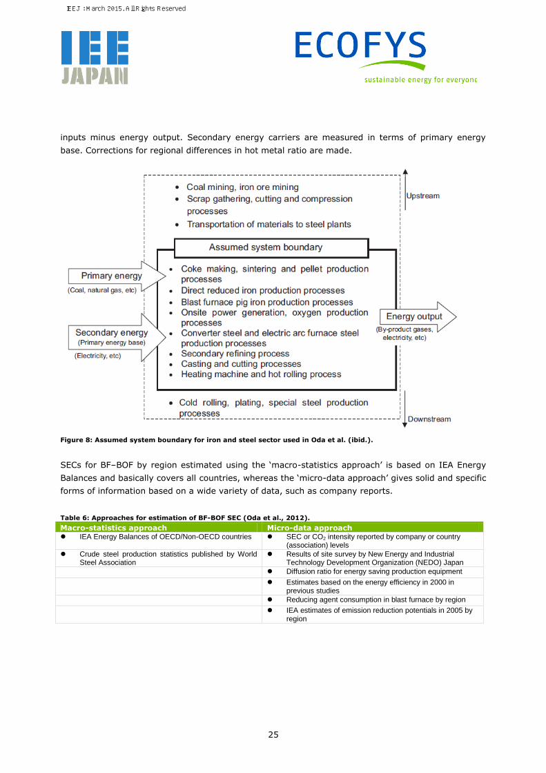
25

inputs minus energy output. Secondary energy carriers are measured in terms of primary energy

base. Corrections for regional differences in hot metal ratio are made.

Figure 8: Assumed system boundary for iron and steel sector used in Oda et al. (ibid.).

SECs for BF–BOF by region estimated using the ‘macro-statistics approach’ is based on IEA Energy

Balances and basically covers all countries, whereas the ‘micro-data approach’ gives solid and specific

forms of information based on a wide variety of data, such as company reports.

Table 6: Approaches for estimation of BF-BOF SEC (Oda et al., 2012).

Macro-statistics approach Micro-data approach IEA Energy Balances of OECD/Non-OECD countries

SEC or CO2 intensity reported by company or country (association) levels

Crude steel production statistics published by World Steel Association

Results of site survey by New Energy and Industrial Technology Development Organization (NEDO) Japan

Diffusion ratio for energy saving production equipment

Estimates based on the energy efficiency in 2000 in previous studies

Reducing agent consumption in blast furnace by region

IEA estimates of emission reduction potentials in 2005 by region


26

4.1.1 Macro-data approach

SECs in BF-BOF steel are estimated using primary energy consumption data from IEA statistics

divided by total crude steel production.

The net energy consumption within the assumed boundary is estimated based on ‘coke ovens’ and

‘blast furnaces’ in energy transformation sector as well as ‘iron and steel sector’ in the energy

demand sector of IEA’s ‘Extended Energy Balances’. ’Coke’ and by-product gases are allocated

between the iron and steel sector and other sectors. Regional share of the net energy consumption

for three routes namely BF-BOF, Scrap-EAF and DRI-EAF is estimated using assumed representative

SECs by route as given in Table 7.

Table 7: Assumed SEC by route for representative value (Oda et al., 2012).

GJ/ton of crude steel Non-electricity Electricity Total

BOF steel 26.2 6.7 32.9

Scrap-EAF steel 2.9 7.3 10.2

DRI-EAF steel 18.1 8.6 26.7

Note: Oda et al. (op cit) estimations refer to a number of earlier studies including reports by the IEA. The value is measured with primary energy base

(LHV). Assumed value of DRI-EAF steel is based on gas-based shaft furnace.

The amount of BF-BOF steel production is estimated using World Steel’s statistics. Regional SECs

estimates of BF-BOF steel using macro-statistics approach are given in Table 8.

Table 8: Estimated SEC in BF–BOF steel in 2005 based on macro-statistics approach (Oda et al., 2012).

GJ/ton of BOF crude steel Estimate based on non-electricity consumption

Estimate based on total consumption

US 30.9 35.5

UK 29.3 26.9

France 26.4 30.6

Germany 24.0 26.4

EU27 25.5 28.8

Japan 23.5 25.7

Korea 28.9 34.2

China 28.6 30.5

India 40.9 30.0

Russia 47.8 65.0

Worldwide total 29.8 32.7

Note: The values are measured with primary energy base (LHV). The hot metal ratio was converted to 1.025. There was no correction for raw material

quality.

4.1.2 Micro-data approach

The micro-data approach is based on a wide variety of data, such as company reports, association

reports, and results of site survey, etc. For the estimation of SEC in China, a more detailed analysis

was conducted based on the energy consumption data provided by large and medium–sized


27

companies to the China Iron and Steel Association. The estimated SEC based on a micro-data

approach is shown in Table 9.

Table 9: Estimated SEC in BF-BOF steel in 2005 based on micro-data approach (Oda et al., 2012).

GJ/ton of BOF crude steel Estimated SEC US 28.9

UK 27.6

France 24.4

Germany 23.6

Belgium, Netherlands 23.8

Japan 23.1

Korea 23.2

India 33.3

Russia 30.3

Note: Oda et al. (op cit) estimations are based on a large amount of literatures. The values are measured in terms of primary energy base (LHV). The

hot metal ratio was converted to 1.025. There was no correction for raw material quality.

4.1.3 Correction for quality of raw materials

As a correction to the differences in the quality of raw materials used in producing countries, three

percentage points are added to energy consumption in Europe, North America, and Brazil, where

Brazilian iron ore which is low in silica and alumina content37 is mainly used, and eight percentage

points are withheld from energy consumption in India due to its high use of ash coal. Both corrections

are made for the purpose of comparing process energy use within the same data boundary.

4.1.4 CO2 emission indicators

Disaggregated energy consumption data by country and production route are required to estimate

CO2 emissions indicator. However, there is no publicly accessible data available currently. Therefore,

the estimation of CO2 emissions indicator for BF-BOF steel is excluded from this analysis.

37 During our hearings with industry experts, it was known that high silica and alumina content has negative effects to oxidation-reduction

reaction of ferrous oxide and thereby increases coke consumptions. Oda et al (ibid.) assumed that an increase of silica and alumina content

leads to a difference of 3% in energy consumption.


28

4.2 Results

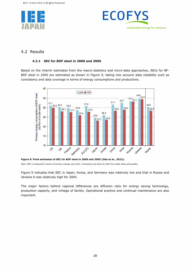
4.2.1 SEC for BOF steel in 2000 and 2005

Based on the interim estimates from the macro-statistics and micro-data approaches, SECs for BF-

BOF steel in 2005 are estimated as shown in Figure 9, taking into account data reliability such as

consistency and data coverage in terms of energy consumptions and productions.

Figure 9: Final estimates of SEC for BOF steel in 2000 and 2005 (Oda et al., 2012).

Note: SEC is measured in terms of primary energy use (LHV). Corrections are done for both hot metal ratios and quality.

Figure 9 indicates that SEC in Japan, Korea, and Germany was relatively low and that in Russia and

Ukraine it was relatively high for 2005.

The major factors behind regional differences are diffusion ratio for energy saving technology,

production capacity, and vintage of facility. Operational practice and continual maintenance are also

important.


29

References

Oda, J., Akimoto, K., Tomoda, T., Nagashima, M., Wada, K., Sano, F., 2012. International

comparisons of energy efficiency in power, steel, and cement industries, Energy Policy 44,

118–129. doi:10.1016/j.enpol.2012.01.024

World Steel, 2014. Steel Statistical Yearbook 2014.

http://www.worldsteel.org/dms/internetDocumentList/statistics-archive/yearbook-

archive/Steel-Statistical-Yearbook-2014/document/Steel-Statistical-Yearbook-2014.pdf


30

Supplementing information: Electric arc furnace

(EAF) in steel sector

EAF accounts for 29% of worldwide crude steel production in 2012 (World Steel, 2014).

Methodology

Oda et al. (ibid.) estimated SEC for Scrap-EAF by region based on the data for each EAF plant

reported by AIST (2010) (Methodology [A]) and based on the improvement ratio of SECs in 2000-

2005 (Methodology [B]).

Methodology [A]

The data of AIST (2010) includes company/location, tap-to-tap time, charged materials (percent of

scrap), and power, oxygen and natural gas consumption of each EAF. In this analysis, oxygen

consumption is converted into primary energy at the ratio of 6.48 MJ/Nm3-O2 in all regions based on

actual electricity consumption using pressure swing adsorption. As AIST (2010) focuses only on EAF

processes, energy consumption in other process, such as secondary refining, casting, and hot rolling

processes, is added. Based on the assumed basic energy consumption by process and the reported

SECs in EAF steelmaking route in the U.S., 3.23 GJ/tcs is assumed for additional energy consumption.

Methodology [B]

As AIST (2010) data is limited to seven countries, Oda et al. (ibid.) applied the improvement ratio for

the period (2000–2005) to SECs for 2000 to derive the SEC for other steel producing countries. The

SECs for 2000 are derived from Oda and Akimoto (2009), which are based on the vintage of EAFs

and the IEA Extended Energy Balances.

To account for a high share of newly installed EAF capacity in total during the period 2000-2005 such

as in India (70%), China (56%) and U.S (22%)38, Oda et al. (ibid.) applied three levels of assumed

SECs for new installation namely 8.0 GJ/tcs for OECD countries; 8.5 GJ/tcs for non-OECD countries

except India; and 9.5 GJ/tcs for India (due to the high share of small-scale induction furnaces) to the

SEC for 2000 to obtain the corresponding SECs for these countries. The outcomes are given as [B2]

in Table Annex-1.

38 Assuming a lifetime of 40-year.


31

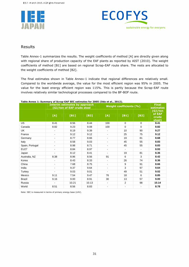
Results

Table Annex-1 summarizes the results. The weight coefficients of method [A] are directly given along

with regional share of production capacity of the EAF plants as reported by AIST (2010). The weight

coefficients of method [B1] are based on regional Scrap-EAF route share. The rests are allocated to

the weight coefficients of method [B2].

The final estimates shown in Table Annex-1 indicate that regional differences are relatively small.

Compared to the worldwide average, the value for the most efficient region was 95% in 2005. The

value for the least energy efficient region was 115%. This is partly because the Scrap-EAF route

involves relatively similar technological processes compared to the BF-BOF route.

Table Annex 1: Summary of Scrap-EAF SEC estimates for 2005 (Oda et al., 2012).

Interim estimates by approach (GJ/ton of EAF crude steel

Weight coefficients (%) Final

estimates (GJ/ton of EAF crude steel)

[A] [B1] [B2] [A] [B1] [B2]

US 8.41 8.56 8.44 100 0 0 8.41

Canada 8.82 9.23 9.08 100 0 0 8.82

UK - 8.19 9.39 - 10 90 9.27

France - 9.12 9.12 - 25 75 9.12

Germany - 8.77 8.66 - 19 81 8.68

Italy - 8.58 9.03 - 45 55 8.83

Spain, Portugal - 8.98 8.71 - 45 55 8.83

EU27 - 8.84 8.97 - - - 8.93

Japan - 8.12 8.41 - 19 81 8.36

Australia, NZ 8.38 8.96 8.56 91 6 3 8.42

Korea - 8.43 8.33 - 26 74 8.36

China - 7.68 8.75 - 9 91 8.66

India - 9.37 9.64 - 3 97 9.64

Turkey - 9.03 9.01 - 49 51 9.02

Mexico 9.11 7.54 9.47 76 18 6 8.85

Brazil 9.16 9.00 8.91 30 13 57 9.00

Russia - 10.21 10.13 - 2 98 10.14

World 8.51 8.56 8.83 - - - 8.78

Note: SEC is measured in terms of primary energy base (LHV).


32

References

Association for Iron and Steel Technology (AIST), 2010. AIST Industry Roundups, EAF Roundup,

2010.

Oda, J., Akimoto, K., 2009. An evaluation of energy efficiency in iron and steel sector. Journal of

Japan Institute of Energy 88, 1009–1016 (in Japanese).

Oda, J., Akimoto, K., Tomoda, T., Nagashima, M., Wada, K., Sano, F., 2012. International

comparisons of energy efficiency in power, steel, and cement industries, Energy Policy 44,

118–129. doi:10.1016/j.enpol.2012.01.024


33

5 Cement

5.1 Overview of the cement manufacturing process

The cement manufacturing process can be divided into the “raw material process”, “calcination

process” and “finishing process”.

The “raw material process” is a process consisting of mixing the main raw materials, such as

limestone, clay, silica, iron raw material, and other raw materials into a specific chemical composition

and granulating them in raw material grinding mill. The resulting material is called “mixed raw

material”. Recently, many types of waste and by-products are widely used as alternative raw

materials.

The “calcination process” is a process to produce clinker by burning the mixed raw materials at high

temperature in rotary kiln. Clinker, an intermediate product is the main component for the

manufacturing of cement. A major portion of energy used in the entire cement production is

consumed during “calcinations process”, which is, in the production of clinker39.

Calcination of clinker takes place in a rotary kiln. Feeding the mixed raw materials to the preheater

before entering the rotary kiln is commonly practiced nowadays to improve calcinations efficiency.

The effective use of industrial and municipal waste as alternative fuel for the kiln is gaining popularity

nowadays.

The “finishing process” is a process where gypsum is added to the clinker and grinded in the finishing

mill. The resulting fine particles are known as the Portland cement. Mixed cement is produced by

mixing the Portland cement and admixtures with a mixer.

5.2 Energy and CO2 indicators in the cement manufacturing process

As mentioned in the previous section, the “calcinations” process is the most energy consuming

process in cement production. Therefore, it is important to focus on the energy efficiency of the

clinker production. In terms of CO2 emissions, it is necessary to take into account the entire cement

manufacturing process including the “calcinations process”.

In addition, the use of an appropriate denominator to derive the energy and CO2 efficiency indicators

for cement industry depends on the types of the target.

39 For example, the breakdown of energy consumption in each of the cement manufacturing process in Japan is as follows: raw material

process (0% heat, 8% electricity); calcination process (72% heat, electricity 8%); and finishing process (0% heat, 12% electricity).


34

In terms of fuel energy reduction target, it is better to focus on fuel efficiency for energy intensive

clinker process which constitutes the major portion of energy use in cement production. Improving

energy efficiency of kiln is the most effective measure for energy efficiency improvement in the

cement industry.

In terms of CO2 emission reduction target, it is better to focus on not only fuel efficiency for clinker

process but also the type of cement composition. Enhancing the use of alternative additives such as

slag and fly ash contributes to lower CO2 emissions from cement production process. The mixing rate

for cement composition depends on quality regulation of cement and the needs or preferences of

consumers which may differ among the regions.

Apart from the above, electricity consumption is also one of the important indicators for cement

industry. Although electricity consumption is generally treated as indirect emission, cement

manufacturing consumes a high level of electricity in particular for grinding, thereby suggesting the

necessity of considering it as one of the performance indicators.

Based on the above discussions, indicators which are deemed suitable to appropriately measure the

efficiency of cement manufacturing process are given in the following.

1. Thermal energy efficiency in clinker manufacturing process

Weighted average thermal energy consumption (excluding heat consumption for alternative fuels)

per tonne clinker in each kiln (MJ / tonne clinker)

This indicator compares the energy efficiency in clinker manufacturing process, the process which

consumes the largest amount of energy in the entire cement manufacturing process. From the view

point of achieving a sustainable society, it is necessary to consider the use of waste materials as

neutral as it reduces the use of fossil fuels as discussed in chapter 5.1, therefore, thermal energy

derived from waste should be excluded in the measurement.

2. CO2 emissions intensity in cement manufacturing

Weighted average net CO2 emission (excluding CO2 emission for alternative fuels) per tonne

cement in each kiln (kg-CO2/tonne cement)

This indicator measures CO2 emissions intensity for the entire cement manufacturing process. Similar

to indicator 1. in the above, the use of waste which would otherwise be incinerated or land filled as

alternative fuel in cement kilns can contribute to the development of a sustainable society as it lowers

overall CO2 emissions by replacing fossil fuels. The net accounting method, which excludes CO2

emissions from waste is desirable to appropriately account for the effective use of waste in cement

manufacturing.

3. Electricity intensity in cement manufacturing

Weighted average electrical power consumption (excluding electricity generated from waste heat)

per tonne cement (kWh/tonne cement)


35

Electricity is one of the main forms of energy consumed in cement manufacturing, thereby suggesting

the need to measure the efficiency of its consumption in production process. For cement plants which

employ waste heat recovery power generation facility, electricity generated from such waste heat

facility should be excluded in the measurement since it offsets a portion of electricity demand in

cement manufacturing.

* Waste heat recovery power generation facility refers to a facility which recovers waste heat from

the preheater exhausts and clinker coolers and uses it to provide low temperature heating needs in

the plant, or in most cases to generate electricity to offset a portion of power purchased from the grid,

or captive power generated by fuel consumption at the site.

The key challenge in developing the energy and CO2 emission indicators for the cement industry is

the poor availability of data. Therefore the approach taken here is to establish indicators using

available data and resource.

5.3 Method

5.3.1 Selection of data

Energy and CO2 indicators for cement industry analysis refers to publicly available “Getting the

Numbers Right (GNR)” database developed by the Cement Sustainability Initiative (CSI) of World

Business Council for Sustainable Development (WBCSD).The WBCSD CSI database is an independent

database of energy and CO2 performance information on the cement industry developed based on a

uniformed system boundary and definitions and has the highest coverage of countries across world

regions40. Consolidated data for country and region are published based on information submitted

annually on plant basis by participating members. Despite the wide differences in coverage across

regions, WBCSD CSI database is perhaps the best publicly available database on the cement industry.

The GNR Data is voluntarily collected by GNR participants for the database using the “CSI-developed

CO2 Accounting and Reporting Standard for the Cement Industry”. The GNR system is intended to

help the cement industry and policymakers alike to better assess the influence of kiln technology, fuel

selection, plant location and other variables on global and regional plant performance and emissions

management.

Countries or region covered are Africa, Asia (excluding China, India, CIS) + Oceania, Brazil, Central

America, China, CIS, Europe, India, Middle East, North America, and South America excluding Brazil

Note that the performance indicators developed by the WBCSD CSI differ from the efficiency

indicators suggested in chapter 5.2 in particular in terms of data boundary. Table 10 summarizes the

key differences between the two:

40 http://wbcsdcement.org/pdf/tf1_co2%20protocol%20v3.pdf


http://wbcsdcement.org/pdf/tf1_co2%20protocol%20v3.pdf

36

Table 10: Differences between the efficiency indicators suggested and WBCSD-CSI database.

I. Efficiency indicator suggested II.WBCSD-CSI data

Differences

Thermal energy efficiency in clinker manufacturing process

Weighted average thermal energy consumption (excluding heat consumption for alternative fuels) per tonne clinker in each kiln (MJ / tonne clinker)

329a Energy consumption (MJ/t) including energy for drying fuels and raw materials MJ / tonne clinker

II includes heat consumption for alternative fuels

CO2 emissions intensity in cement manufacturing

Weighted average net CO2 emission (excluding CO2 emission for alternative fuels) per tonne cement (kg-CO2/tonne cement)

326b Weighted average net CO2 emission per tonne cement equivalent in each region over time (excluding CO2 from electric power) (kg CO2 / tonne cement equivalent calculated at company level)

The numerator of indicator II excludes CO2 emission from on-site power generation while the denominator includes clinker bought from third parties for the production of cement

Electricity intensity in cement manufacturing

Weighted average electrical power consumption (excluding from waste heat power generation) per tonne cement (kWh/tonne cement)

3212b Weighted average power consumption for cement manufacturing per tonne of cement in each region over time (kWh / tonne cement)

II includes electricity generated from waste heat

5.3.2 GNR indicator

The following presents the indicators available in the GNR database and its calculation methods:

1. Weighted average thermal energy consumption (including energy for drying fuels and raw

materials) per tonne clinker in each region (MJ / tonne clinker)

The indicator is calculated by total heat consumption of kilns (MJ, year) including heat consumption

for drying fuels and raw materials in the region divided by production of clinker (tonne, year) in the

region.

2. Weighted average net CO2 emission per tonne cement equivalent in each region over time (kg

CO2 / tonne cement equivalent calculated at company level)

The indicator is calculated by total net CO2 emission in the region (kgCO2, year) divided by cement

equivalent production (tonne, year) in the region.

*Net CO2 emissions are calculated by the gross emissions minus the CO2 emissions from alternative

fossil fuels.

where, Gross CO2 emissions include total fossil and direct CO2 emissions from a cement plant or

company. It excludes CO2 emissions from on-site electricity production. Gross emissions also include

CO2 from alternative fossil fuels, but exclude CO2 from biomass fuels and the biomass content of

mixed fuels, since these emissions are regarded as climate-neutral.


37

Note that cement equivalent is the sum of all cements and clinker produced by a cement company,

including clinker purchased from third parties and used to make cement.

3. Weighted average power consumption for cement manufacturing per tonne of cement (kWh /

tonne cement）

The indicator is calculated by power consumption (kWh, year) for cement and clinker production

divided by cement and cement substitute production (tonne, year).

Note that “cement and cement substitute production” excludes clinker sold but includes clinker

bought.


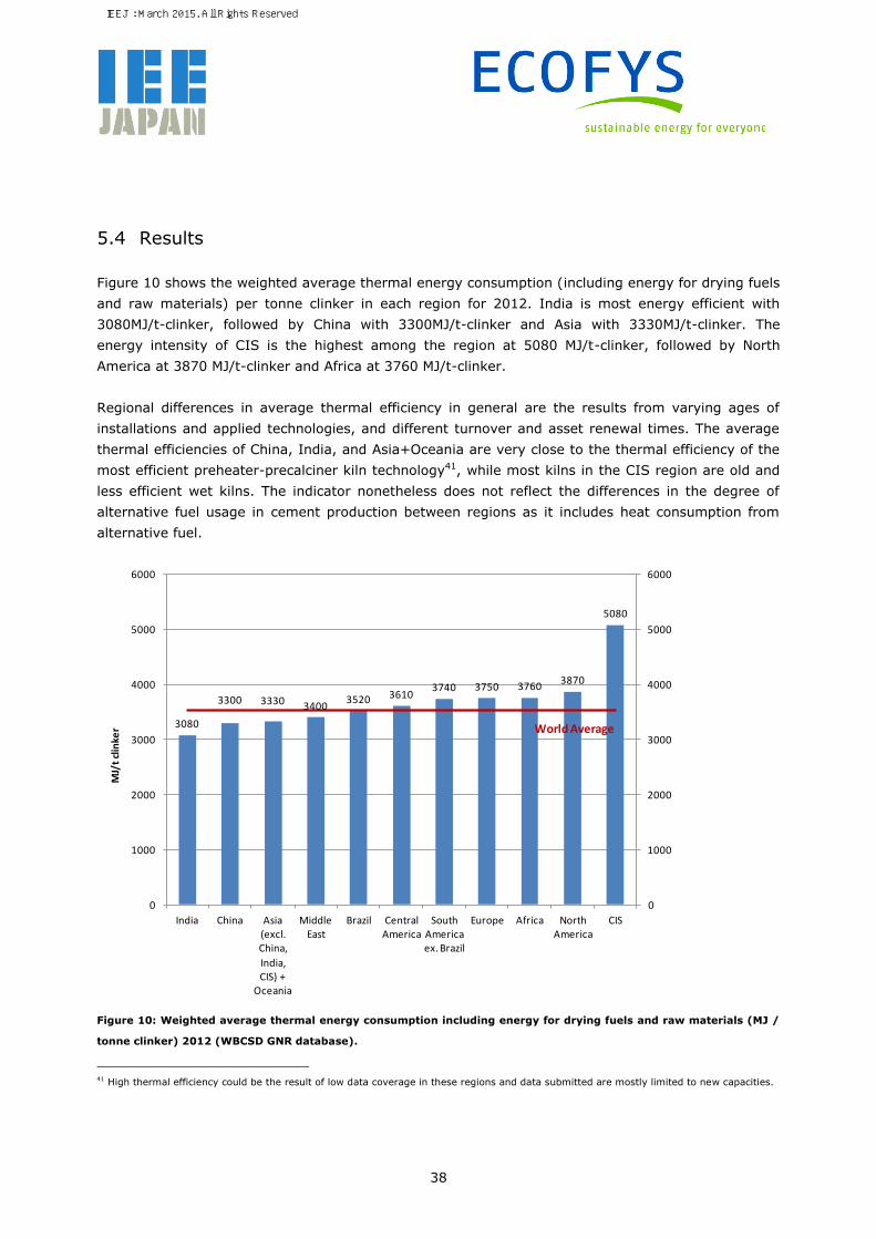
38

5.4 Results

Figure 10 shows the weighted average thermal energy consumption (including energy for drying fuels

and raw materials) per tonne clinker in each region for 2012. India is most energy efficient with

3080MJ/t-clinker, followed by China with 3300MJ/t-clinker and Asia with 3330MJ/t-clinker. The

energy intensity of CIS is the highest among the region at 5080 MJ/t-clinker, followed by North

America at 3870 MJ/t-clinker and Africa at 3760 MJ/t-clinker.

Regional differences in average thermal efficiency in general are the results from varying ages of

installations and applied technologies, and different turnover and asset renewal times. The average

thermal efficiencies of China, India, and Asia+Oceania are very close to the thermal efficiency of the

most efficient preheater-precalciner kiln technology41, while most kilns in the CIS region are old and

less efficient wet kilns. The indicator nonetheless does not reflect the differences in the degree of

alternative fuel usage in cement production between regions as it includes heat consumption from

alternative fuel.

Figure 10: Weighted average thermal energy consumption including energy for drying fuels and raw materials (MJ /

tonne clinker) 2012 (WBCSD GNR database).

41 High thermal efficiency could be the result of low data coverage in these regions and data submitted are mostly limited to new capacities.

3080

3300 3330 34003520 3610

3740 3750 37603870

5080

0

1000

2000

3000

4000

5000

6000

0

1000

2000

3000

4000

5000

6000

India China Asia (excl. China,

India, CIS) +

Oceania

Middle East

Brazil Central America

South America ex. Brazil

Europe Africa North America

CIS

MJ/

t cl

inke

r World Average


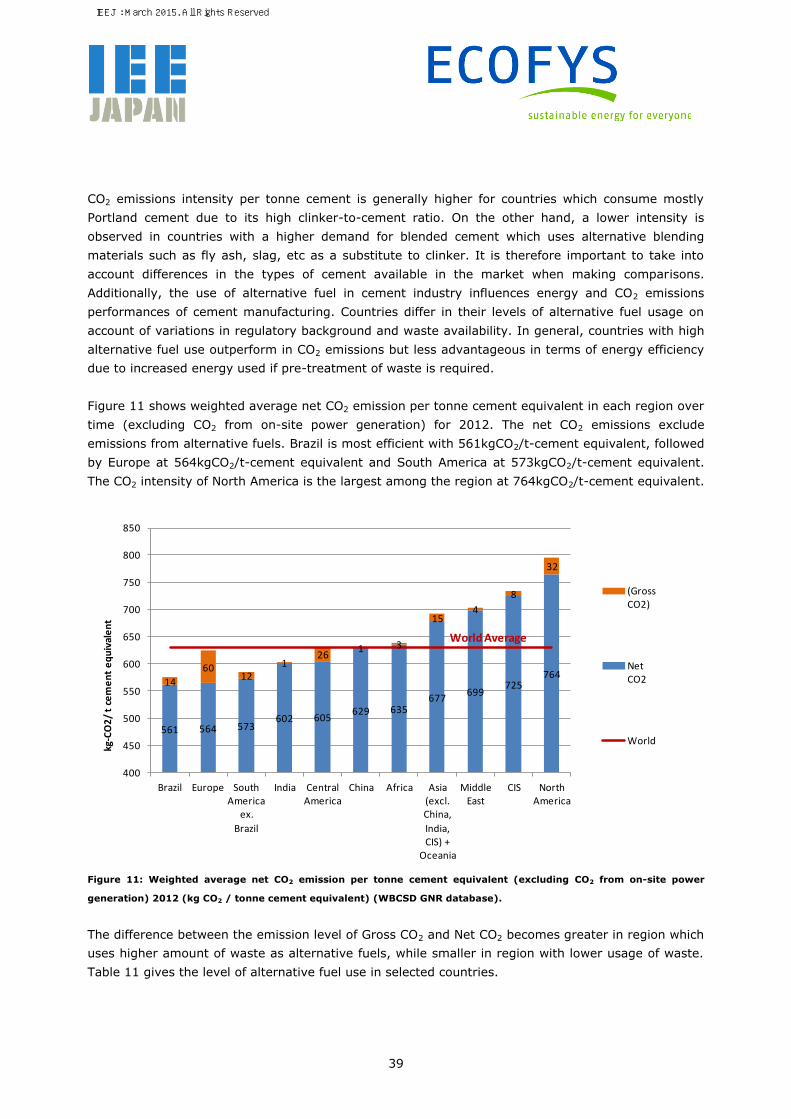
39

CO2 emissions intensity per tonne cement is generally higher for countries which consume mostly

Portland cement due to its high clinker-to-cement ratio. On the other hand, a lower intensity is

observed in countries with a higher demand for blended cement which uses alternative blending

materials such as fly ash, slag, etc as a substitute to clinker. It is therefore important to take into

account differences in the types of cement available in the market when making comparisons.

Additionally, the use of alternative fuel in cement industry influences energy and CO2 emissions

performances of cement manufacturing. Countries differ in their levels of alternative fuel usage on

account of variations in regulatory background and waste availability. In general, countries with high

alternative fuel use outperform in CO2 emissions but less advantageous in terms of energy efficiency

due to increased energy used if pre-treatment of waste is required.

Figure 11 shows weighted average net CO2 emission per tonne cement equivalent in each region over

time (excluding CO2 from on-site power generation) for 2012. The net CO2 emissions exclude

emissions from alternative fuels. Brazil is most efficient with 561kgCO2/t-cement equivalent, followed

by Europe at 564kgCO2/t-cement equivalent and South America at 573kgCO2/t-cement equivalent.

The CO2 intensity of North America is the largest among the region at 764kgCO2/t-cement equivalent.

Figure 11: Weighted average net CO2 emission per tonne cement equivalent (excluding CO2 from on-site power

generation) 2012 (kg CO2 / tonne cement equivalent) (WBCSD GNR database).

The difference between the emission level of Gross CO2 and Net CO2 becomes greater in region which

uses higher amount of waste as alternative fuels, while smaller in region with lower usage of waste.

Table 11 gives the level of alternative fuel use in selected countries.

561 564 573602 605

629 635677

699725

76414

6012

126

1 3

154

8

32

400

450

500

550

600

650

700

750

800

850

Brazil Europe South America

ex.

Brazil

India Central America

China Africa Asia (excl. China,

India, CIS) +

Oceania

Middle East

CIS North America

kg-C

O2

/ t

cem

en

t e

qu

ival

en

t

(Gross CO2)

Net CO2

World

World Average


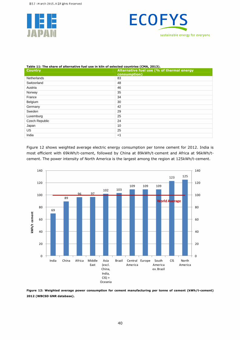
40

Table 11: The share of alternative fuel use in kiln of selected countries (CMA, 2013).

Country Alternative fuel use (% of thermal energy consumption)

Netherlands 83

Switzerland 48

Austria 46

Norway 35

France 34

Belgium 30

Germany 42

Sweden 29

Luxemburg 25

Czech Republic 24

Japan 10

US 25

India <1

Figure 12 shows weighted average electric energy consumption per tonne cement for 2012. India is

most efficient with 69kWh/t-cement, followed by China at 89kWh/t-cement and Africa at 96kWh/t-

cement. The power intensity of North America is the largest among the region at 125kWh/t-cement.

Figure 12: Weighted average power consumption for cement manufacturing per tonne of cement (kWh/t-cement)

2012 (WBCSD GNR database).

69

89 96 97

102 103 109 109 109

123 125

0

20

40

60

80

100

120

140

0

20

40

60

80

100

120

140

India China Africa Middle East

Asia (excl. China,

India, CIS) +

Oceania

Brazil Central America

Europe South America ex. Brazil

CIS North America

kWh

/t c

em

en

t

World Average


41

5.5 Discussion

The situation surrounding cement industry varies in each region and this lead to variation in results

depending on the indicators measured. The outcomes suggest the need to compare not only one but

several indicators for the following reasons. Careful consideration is also required in selecting the

appropriate denominator and indicator for international comparison.

1. Data availability and boundary

Apart from European Cement Association (CEMBUREAU) and the Inter-American Cement Federation

(FICEM) which share their database with GNR, worldwide database on cement industry is currently

not publicly available. Further discussions are deemed necessary as significant uncertainty exists

around the results presented in this analysis due to the absence of comprehensive data for countries

like Japan, India, etc.

The compilation of energy and CO2 indicators for cement industry are subject to the availability of

various data including detailed energy consumption data for each process of clinker and cement

production. Although the WBCSD CSI database is referred in this analysis, note that the coverage

varies widely across regions. Additionally, it may be necessary to analyze changes in trends over a

selected period of time to exclude annual irregularities.

The collection of national data for cement industry differs between countries and the quality of data is

not always the same due to differences in definition and system boundary. The establishment of a

reliable, comparable and highly transparent database for the cement industry requires close

cooperation between respective organizations and authority in-charge among countries.

2. Definition used for cement products

The appropriate data to be used as the denominator differs depending on the operational

characteristic of a cement plant. For example, in some countries clinker is produced in the same

cement plant whereas in other countries, the production of clinker takes place at a facility separate to

the cement plant. The “cement equivalent” denominator referred in this analysis is defined by the

GNR database as the sum of all cements and clinker produced by a cement company including clinker

purchased from third parties but excluding clinker sold. The definition suggests the tendency for a

cement plant which purchases clinker from third parties to have lower energy intensity. On the other

hand, “cementitious products” which is not referred in this analysis covers all alternative raw

materials such as slag produced and sold to third parties but excludes clinker bought. In this case,

cement plant with a large quantity of sales tends to have a smaller intensity. Caution must therefore

be exercised in selecting the appropriate denominator considering its limitations from available data.

3. Energy efficiency in cement manufacturing process

The selection of appropriate indicators for cement industry is essentially the choice of indicators

which could best measure the efficiency of a facility. Perhaps the most appropriate indicator from an

energy efficiency point of view is the thermal energy efficiency in clinker manufacturing process since


42

this is the most energy consuming process in entire cement production process. Ideally, energy from

waste and biomass should be excluded in the evaluation on account of their contributions towards

achieving a sustainable society.

4. Specific CO2 emission

As explained above, Net CO2 emission is calculated by Gross CO2 emission subtracted with emission

from alternative fuels such as waste oil, used tires, plastics, solvents, and bottom sludge. Therefore,

the difference in number between Net CO2 emission and Gross CO2 emission is derived by the amount

of waste used as an alternative energy source which varies widely across regions. Thus, the

difference between the emission level of Gross CO2 and Net CO2 becomes greater in the region which

uses larger amount of waste as alternative fuels, while smaller in the region with lower usage of

waste.

It is noted that the amount of waste use in the region varies and is mainly influenced by the level of

development of waste legislation, law enforcement, waste collection infrastructure, and local

environmental awareness.

5. Specific power consumption

Although electricity consumption is treated as indirect emissions, the use of electricity in cement

production is significant, thereby suggesting its importance as one of the performance indicators for

cement industry. The efficiency of electricity consumption of cement plant is best measured by taking

into account the entire cement manufacturing process and excluding electricity generated from waste

heat recovery power generation facility since it offsets a portion of electricity demand in cement

manufacturing. It is anticipated that more than 15% of electricity demand could be met by the

efficient use of waste heat in cement kilns.


43

5.6 Glossary

Perimeter of CO2 emissions considered: only direct CO2 emissions related to the production of

cement and clinker, excluding on-site electricity production.

Gross CO2 emissions: direct CO2 emissions (excluding on-site electricity production) minus

emissions from biomass fuel sources.

Net CO2 emissions: gross CO2 emissions minus emissions from alternative fossil fuels.

Alternative fuels: fuels used for fossil fuel substitution in clinker production. Alternative fuels

are derived from waste (excluding biomass waste).

Clinker: intermediate product in cement manufacturing. Clinker is the result of calcination of

raw materials in the kiln.

Cement: finished product of the cement plant obtained by grinding the clinker and adding

various components (gypsum, limestone).

Cement equivalent is the sum of all cements and clinker produced by a cement company,

including clinker purchased from third parties and used to make cement.

Cementitious products are all clinker volumes produced by a company for cement making or

direct clinker sale, plus gypsum, limestone, CKD, and all clinker substitutes consumed for

blending, plus all cement substitutes produced. Clinker bought from third parties for the

production of cement is excluded.


44

References

Cement Sustainability Initiative, WBCSD. “Getting the Numbers Right (GNR)”.

http://wbcsdcement.org/index.php/key-issues/climate-protection/gnr-database

WBCSD (2011). CO2 and Energy Accounting and Reporting Standard for the Cement Industry.

http://wbcsdcement.org/pdf/tf1_co2%20protocol%20v3.pdf

Izumi Y (2014). Role of the Japanese Cement Industry in the Establishment of a Sustainable Society.

Key Engineering Materials, vol. 617:50-58.

Cement Manufacturers' Association India, CMA (2013). Status of AFR in India.


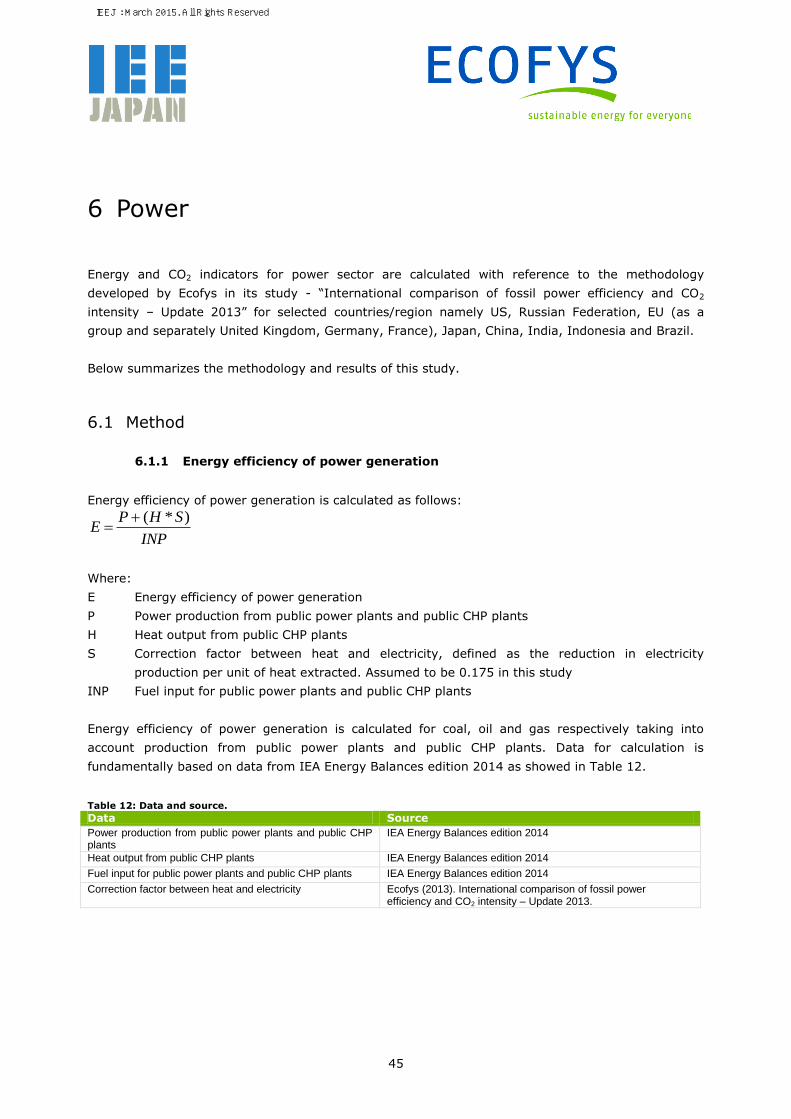
45

6 Power

Energy and CO2 indicators for power sector are calculated with reference to the methodology

developed by Ecofys in its study - “International comparison of fossil power efficiency and CO2

intensity – Update 2013” for selected countries/region namely US, Russian Federation, EU (as a

group and separately United Kingdom, Germany, France), Japan, China, India, Indonesia and Brazil.

Below summarizes the methodology and results of this study.

6.1 Method

6.1.1 Energy efficiency of power generation

Energy efficiency of power generation is calculated as follows:

INP

SHPE

)*(

Where:

E Energy efficiency of power generation

P Power production from public power plants and public CHP plants

H Heat output from public CHP plants

S Correction factor between heat and electricity, defined as the reduction in electricity

production per unit of heat extracted. Assumed to be 0.175 in this study

INP Fuel input for public power plants and public CHP plants

Energy efficiency of power generation is calculated for coal, oil and gas respectively taking into

account production from public power plants and public CHP plants. Data for calculation is

fundamentally based on data from IEA Energy Balances edition 2014 as showed in Table 12.

Table 12: Data and source.

Data Source

Power production from public power plants and public CHP plants

IEA Energy Balances edition 2014

Heat output from public CHP plants IEA Energy Balances edition 2014

Fuel input for public power plants and public CHP plants IEA Energy Balances edition 2014

Correction factor between heat and electricity Ecofys (2013). International comparison of fossil power efficiency and CO2 intensity – Update 2013.


46

6.1.2 CO2 intensity of power generation

CO2 intensity for power generation is calculated for each country by fuel and for total fossil power

generation. The calculation uses the same method as for calculating energy efficiency where heat

generation is corrected by correction factor of 0.175. Table 13 summarizes the data used and its

sources for the calculation of CO2 intensity.

The formula for calculating CO2 intensity is as follows:

CO2i = Ci / Pi

Where:

CO2i CO2 intensity

i Fuel source 1 … n

Ci CO2 emission per fuel source (tonCO2)

Pi Power production from public power and CHP plants per fuel source (MWh)

Table 13: Data and source.

Data Source

CO2 emission per fuel source IEA CO2 emissions from fuel combustion edition 2014

Power production from public power and CHP plants per fuel source

IEA Energy Balances edition 2014


47

6.2 Results

6.2.1 Average efficiency of power generation

Figure 13 shows average energy efficiency of fossil-fired power generation in 2012. Country wise

differences in energy efficiency are large with Japan leading ahead at 44% followed by United

Kingdom and Brazil, whereas country like India achieved a low 27.6% due to its high dependency on

inefficient coal-fired power generation. China on the other hand recorded an average efficiency of

35.7%, up from 34.8% in 200942. The improvements come mostly from its coal power plant which

has increased steadily in the period 1990 to 2012 and accounted for close to 80% of total power

generated in 2011. Japan leads amongst the countries covered for the analysis on account of the use

of advanced combined cycle technology in newly built and replacement of aging gas-fired power

plants in recent years.

Figure 13: Average efficiency of fossil-fired power generation (2012) (compiled from IEA data).

Efficiency of coal-fired power generation ranged from 26.6% for India to 40.7% in the case of Japan

in 2012 (Figure 14). Of all countries covered, China and Russia achieved a significant progress in

efficiencies of its coal power plant facilities since 1990 while other countries have experienced limited

improvement. Thermal efficiency for China has increased from 28.9% in 1990 to 35.7% at present.

As for Russia, efficiency was 31.3% in 2012, up from 20.8% in 1990. Nonetheless, this is still

substantially below industry benchmarks.

42 Ecofys (2013). International comparison of fossil power efficiency and CO2 intensity – Update 2013.

44.0%42.7% 41.7% 41.0% 40.4% 40.0% 39.1%

35.7%33.3%

31.5%

27.6%

0%

10%

20%

30%

40%

50%

Japan United Kingdom

Brazil United States

EU28 Germany France China Indonesia Russian Federation

India

Eff

icie

ncy

(%)

Average efficiency of fossil-fired power generation (2012)


48

Figure 14: Efficiency of coal-fired power generation (2012) (compiled from IEA data).

For gas power plants, thermal efficiencies have generally improved in all countries except in China,

on account of its relatively small share in generation mix43 (Figure 15). The range of efficiency for

countries is wide with 31.5% for Russia and 51.8% for United Kingdom. Russia obtains about 45% of

its power needs from gas, mostly from combined heat and power plants, which is superior to a

system that relies upon separate boilers and power plants. Average efficiency is well below sector

average and far away from 59.3% for a modern combined cycle gas turbine plants. Its low efficiency

is a result of limited investment in this sector since the collapse of the economy during the Soviet

times, where 40% of its thermal power capacity is more than 40 years old.

43 Please note that gas-fired power generation accounts for less than 2% of total electricity generated in 2012 and its thermal efficiency has

remained constant since 1990.

40.7%38.9% 38.7%

37.4% 37.0% 36.9%35.7%

31.3% 30.7%29.6%

26.6%

0%

5%

10%

15%

20%

25%

30%

35%

40%

45%

Japan United Kingdom

Germany EU28 France United States

China Russian Federation

Indonesia Brazil India

Effi

cien

cy (%

)

Efficiency of coal-fired power generation (2012)


49

Figure 15: Efficiency of gas-fired power generation (2012) (compiled from IEA data).

6.2.2 CO2 intensity of power generation

Figure 16 compares country wise CO2 intensity for fossil fuel-fired power generation in 2012. CO2

intensity for fossil fuel-fired power generation ranges from 590gCO2/kWh for Brazil to 1181g

CO2/kWh for India. Japan comes at the second lowest at 615gCO2/kWh for 2012. The share of coal,

which has a larger CO2 emission factor in power generation mix and generation efficiency influence

the CO2 intensity for fossil fuel-fired power generation. India emits 1181gCO2 for every unit of

electricity generated, almost double of that in Brazil. This is again due to the dominating role of coal-

fired power generation in its energy mix. Compared to Japan, countries like China emit 50% more in

emissions per unit of power generated from fossil fuel power plants.

51.8%49.9% 48.7% 48.2% 47.7% 47.0% 45.9%

43.0%

38.9%37.2%

31.5%

0.0%

10.0%

20.0%

30.0%

40.0%

50.0%

60.0%

United Kingdom

Brazil EU28 United States

Japan Germany India France China Indonesia Russian Federation

Effi

cien

cy (%

)

Efficiency of gas-fired power generation (2012)


50

Figure 16: CO2 intensity for fossil fuel-fired power generation (2012) (compiled from IEA data).

Figure 17 shows country wise CO2 intensity for coal-fired power generation in 2012. CO2 intensity for

coal-fired power generation ranges from 857gCO2/kWh for United Kingdom to 1256gCO2/kWh for

India, a difference of 47% in emissions per unit of electricity generated.

Figure 17: CO2 intensity for coal-fired power generation (2012) (compiled from IEA data).

590 615

689 705 752 758 760

815 865

927

1181

0

200

400

600

800

1000

1200

1400

Brazil Japan United Kingdom

United States

France Russian Federation

EU28 Germany Indonesia China India

CO

2 in

ten

sity

(g/k

Wh

)

CO2 intensity for fossil fuel-fired power generation (2012)

857 889 904 915 929 936

1017

1095 1104 1171

1256

0

200

400

600

800

1000

1200

1400

United Kingdom

Japan Germany United States

EU28 China France Russian Federation

Indonesia Brazil India

CO

2 in

ten

sity

(g/k

Wh

)

CO2 intensity for coal fuel-fired power generation (2012)


51

Figure 18 shows country wise CO2 intensity for gas-fired power generation in 2012. CO2 intensity for

gas-fired power generation ranges from 388gCO2/kWh for United Kingdom to 638gCO2/kWh for

Russia, a difference of 64% in emissions per unit of electricity generated.

Figure 18: CO2 intensity for gas-fired power generation (2012) (compiled from IEA data).

388 403 412 417 421 428 438

467

517 540

638

0

100

200

300

400

500

600

700

United Kingdom

Brazil EU28 United States

Japan Germany India France China Indonesia Russian Federation

CO

2 in

ten

sity

(g/k

Wh

)

CO2 intensity for gas fuel-fired power generation (2012)


52

References

Ecofys, 2013. International comparison of fossil power efficiency and CO2 intensity – Update 2013.

IEA, 2014. Energy Balances for OECD and non-OECD countries edition 2014.

IEA, 2014. CO2 emissions from fuel combustion edition 2014.

The Federation of Electric Power Companies of Japan homepage.

http://www.fepc.or.jp/environment/warming/co2_taisaku/fire/index.html (in Japanese).


53

7 Transport

In this analysis, energy consumption efficiency for transport sector refers to Global Fuel Efficiency

Initiative, GFEI’s study in “International Comparison of Light-Duty Vehicle Fuel Economy and Related

Characteristics” (GFEI, 2011), and the following updated paper of GFEI (2013) of “International

comparison of light-duty vehicle fuel economy: An update using 2010 and 2011 new registration

data”, where fuel efficiency of LDV, mainly passenger vehicles, are compared for various countries,

including Japan, EU27, United States, China, India, South Africa, Brazil, Indonesia, Russian, France,

Germany and United Kingdom.

Due to data availability, this analysis focuses on light-duty vehicle (LDV). It does not cover the whole

road sector and exclude other transport sectors such as aviation, railway, shipping and pipeline from

the analysis. Considering the large energy consumption of LDV relative to total energy requirement of

road sector and transport sector44 as a whole, the analysis on LDV can be regarded as a good start in

comparing the efficiency of transport sector.

Below summarizes the methodology and results of this study.

7.1 Method

GFEI’s report estimates the fuel economy characteristics for recently registered vehicles (2005, 2008,

2010 and 2011) in countries with available data.

7.1.1 Data sources

Based on Polk Inc’s database, which includes number of registrations and vehicle characteristics for

various vehicle types at the manufacturer/model/configuration level of detail, IEA/GFEI added the

database with fuel economy test data, using a range of sources containing official tested fuel

economy for vehicle models sold in 2005, 2008, 2010 and 2011. Only the US and Japan have

separate test cycle in the set of countries covered and all others report fuel economy using the

European NEDC (New European Driving Cycle) test cycle (Table 14).

44 Due to its large energy consumption relative to total fuel consumed by the transport sector, CO2 emission from road sector is anticipated

to account for around 75% of total emissions from the transport sector. In addition, detailed CO2 emissions data covering only LDV is not

available. Nonetheless, IEEJ estimated that passenger vehicle accounts for 57.8% of road’s energy consumption in 2010, for the same

regions covered in this analysis.


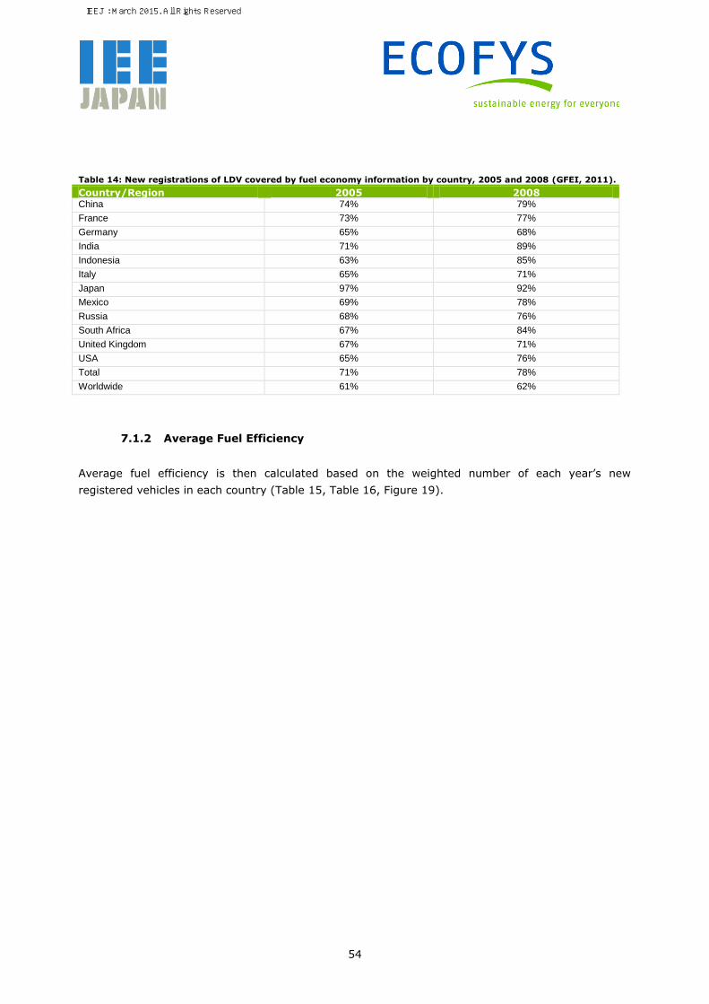
54

Table 14: New registrations of LDV covered by fuel economy information by country, 2005 and 2008 (GFEI, 2011).

Country/Region 2005 2008 China 74% 79%

France 73% 77%

Germany 65% 68%

India 71% 89%

Indonesia 63% 85%

Italy 65% 71%

Japan 97% 92%

Mexico 69% 78%

Russia 68% 76%

South Africa 67% 84%

United Kingdom 67% 71%

USA 65% 76%

Total 71% 78%

Worldwide 61% 62%

7.1.2 Average Fuel Efficiency

Average fuel efficiency is then calculated based on the weighted number of each year’s new

registered vehicles in each country (Table 15, Table 16, Figure 19).


55

7.2 Results

7.2.1 Fuel efficiency comparison for passenger vehicles (2005, 2008)

Table 15: Fuel Efficiency Comparison for Passenger Vehicles (2005, 2008) (Unit: Lge/100km) (GFEI, 2011).

Country/Region 2005 2008 Test cycle

Japan 6.7 6.2 10-15

EU27 7.0 6.6 NEDC

United States 9.7 9.1 FTP

China 7.8 8.1 NEDC

India 5.6 6.1 NEDC

South Africa 7.7 7.6 NEDC

Brazil 7.3 7.4 NEDC

Indonesia 7.2 7.3 NEDC

Russia 8.3 8.1 NEDC

France 6.6 6.0 NEDC

Germany 7.5 7.1 NEDC

UK 7.3 6.8 NEDC

Note 1: Lge is Liter of gasoline equivalent; 10-15 is the test mode used in Japan. NEDC is New European Driving Cycle commonly used in the Europe;

FTP is the Federal Test Procedures in US.

Note 2: The above figures are so called fuel efficiency for different test mode, which is usually different from the on-road fuel efficiency.

Note 3: Though it is difficult to make direct comparisons among the figures derived using varying cycle modes, these results are still informative as they

are designed to reflect the actual efficiency as much as possible.

7.2.2 Fuel efficiency comparison for passenger vehicles (2010, 2011)

Table 16: Fuel Efficiency Comparison for Passenger Vehicles (2010, 2011) (GFEI, 2013).

Country/Region 2010 (gCO2/km) 2011 (gCO2/km) 2010 (Lge/100 km) 2011 (Lge/100 km)

Japan 140.5 134.4 6.0 5.8

EU27 140.3 135.7 6.0 5.8

United States 194.7 192.8 8.3 8.2

China - - - -

India - - - -

South Africa - - - -

Brazil - - - -

Indonesia - - - -

Russia - - - -

France 130.5 127.7 5.6 5.5

Germany 151.2 145.6 6.5 6.2

UK 144.2 138.1 6.2 5.9

Note: Data in the first two columns are original data in GFEI (2013). Data in the last two columns are converted to Lge/100km by IEEJ based on ICCT’s

(2014) conversion methods. The conversion is intended to present vehicles’ efficiency expressed in unit of fuel consumption, assuming that it is a

gasoline vehicle.


56

Figure 19: Fuel Efficiency Comparison for Passenger Vehicles (LDV) from 2005 to 2011 (GFEI, 2013).

As can be seen from the above tables and figures, several conclusions can be drawn.

Although not all new registration vehicles have fuel economy information, but the database

has a reasonable high coverage. As the result, for most countries, the difference between

country’s official figures and the above GFEI’s results are within several percentages (GFEI,

2011).

The fuel economy of all our concerned countries is improving from 2005 to 2011.

For 2008, top three high efficient markets are India, Japan and EU27.

For 2010 and 2011, both Japan and EU27 have improved their fuel efficiency, with EU27

catching up with Japan.

The difficulties to compare energy efficiency in transport sector arise from the world-wide

data availability, as well as different test modes.

Comparing fuel efficiency based on vehicle stock or actual on-road efficiency is more

challenging. It is therefore an important first step to compare fuel efficiency of new vehicles.


57

References

GFEI, 2011. International Comparison of Light-Duty Vehicle Fuel Economy and Related Characteristics,

IEA, Paris.

www.globalfueleconomy.org/Documents/Publications/wp5_iea_fuel_Economy_report.pdf

GFEI, 2013. International comparison of light-duty vehicle fuel economy: An update using 2010 and

2011 new registration data.

http://www.globalfueleconomy.org/documents/publications/wp8_international_comparison.p

df

ICCT, 2014. Global passenger vehicle standards. http://www.theicct.org/info-tools/global-passenger-

vehicle-standards


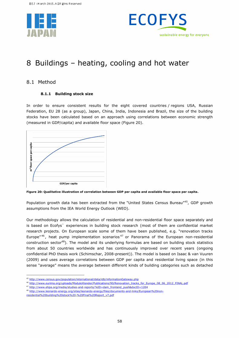
58

8 Buildings – heating, cooling and hot water

8.1 Method

8.1.1 Building stock size

In order to ensure consistent results for the eight covered countries / regions USA, Russian

Federation, EU 28 (as a group), Japan, China, India, Indonesia and Brazil, the size of the building

stocks have been calculated based on an approach using correlations between economic strength

(measured in GDP/capita) and available floor space (Figure 20).

Figure 20: Qualitative illustration of correlation between GDP per capita and available floor space per capita.

Population growth data has been extracted from the “United States Census Bureau”45, GDP growth

assumptions from the IEA World Energy Outlook (WEO).

Our methodology allows the calculation of residential and non-residential floor space separately and

is based on Ecofys` experiences in building stock research (most of them are confidential market

research projects. On European scale some of them have been published, e.g. “renovation tracks

Europe” 46 , heat pump implementation scenarios 47 or Panorama of the European non-residential

construction sector48). The model and its underlying formulas are based on building stock statistics

from about 50 countries worldwide and has continuously improved over recent years (ongoing

confidential PhD thesis work (Schimschar, 2008-present)). The model is based on Isaac & van Vuuren

(2009) and uses average correlations between GDP per capita and residential living space (in this

sense “average” means the average between different kinds of building categories such as detached

45 http://www.census.gov/population/international/data/idb/informationGateway.php 46 http://www.eurima.org/uploads/ModuleXtender/Publications/90/Renovation_tracks_for_Europe_08_06_2012_FINAL.pdf 47 http://www.ehpa.org/media/studies-and-reports/?eID=dam_frontend_push&docID=1204 48 http://www.leonardo-energy.org/sites/leonardo-energy/files/documents-and-links/European%20non-

residential%20building%20stock%20-%20Final%20Report_v7.pdf


http://www.census.gov/population/international/data/idb/informationGateway.php

http://www.eurima.org/uploads/ModuleXtender/Publications/90/Renovation_tracks_for_Europe_08_06_2012_FINAL.pdf

http://www.ehpa.org/media/studies-and-reports/?eID=dam_frontend_push&docID=1204

http://www.leonardo-energy.org/sites/leonardo-energy/files/documents-and-links/European%20non-residential%20building%20stock%20-%20Final%20Report_v7.pdf

http://www.leonardo-energy.org/sites/leonardo-energy/files/documents-and-links/European%20non-residential%20building%20stock%20-%20Final%20Report_v7.pdf

59

and attached single and multi-family houses from different world regions). In a second step, typical

correlations between the residential and non-residential floor space are used (we have found out that

there are typical correlations between the residential and non-residential floor space per capita and

GDP per capita. Such correlations are currently still investigated within the ongoing confidential PhD

thesis work of Schimschar (Schimschar, 2008). For the project, the residential and non-residential

floor space have been aggregated. The non-residential building sector comprises the following

building categories:

Offices

Wholesale and retail trade

Education

Hotels and restaurants

Health and social work

Other

Not included are industrial floor spaces, warehouses and agricultural floor spaces.

8.1.2 Total energy consumption

Information on total energy consumption in the eight countries has been extracted from IEA energy

balances for the year 2012. The IEA provides data for the residential sector as well as for the

commercial and public services sector which is assumed to cover all non-residential services relevant

for the purpose of this study (see covered building categories above). Based on this data and the

calculated floor area it is possible to calculate the specific average energy consumption per square

metre for all residential and non-residential buildings as well as the weighted average.

8.1.3 Total emissions

For the calculation of the CO2 emissions in the building sector, the following emission factors have

been used:

Table 17: CO2 emission factors used for the calculation of the emissions in the building sector.

Coal

Gas/ Diesel / fuel oil + Motor gasoline

Kero-sine

Natural Gas

LPG +

Natural gas liquids

District heat

Geo-

thermal, solar etc

Combustion renewable & waste

Electricity

Unit MtCO2

/TWh

MtCO2

/TWh

MtCO2

/TWh

MtCO2

/TWh

MtCO2

/TWh

MtCO2

/TWh

MtCO2

/TWh

MtCO2 /TWh MtCO2 /TWh

European Union 28

0.341 0.267 0.259 0.202 0.227 0.361 0 0 0.389

Brazil 0.341 0.267 0.259 0.202 0.227 0.068 0 0 0.068

China 0.341 0.267 0.259 0.202 0.227 0.711 0 0 0.764

India 0.341 0.267 0.259 0.202 0.227 0.856 0 0 0.856

Indonesia 0.341 0.267 0.259 0.202 0.227 0.755 0 0 0.755

Japan 0.341 0.267 0.259 0.202 0.227 0.495 0 0 0.497

Russian Federation

0.341 0.267 0.259 0.202 0.227 0.332 0 0 0.437

United States

0.341 0.267 0.259 0.202 0.227 0.495 0 0 0.503


60

The emission factors for coal, oil, kerosene, natural gas and LPG have been extracted from 2006 IPCC

Guidelines for National Greenhouse Gas Inventories (Volume 2: Energy - Chapter 2: Stationary

Combustion, Table 2.5 (IPCC, 2006)). The district heat and electricity factors for each country are

extracted from the IEA while for all kinds of renewable energies, an emission factor of zero has been

used, as discussed with IEEJ.

8.1.4 Separation by space heating, hot water and space cooling

To allow separating the total residential energy consumption into the different energy uses, the

following priority list of use types has been developed which reflects the importance for the

residential occupants:

1) Cooking

2) Refrigeration

3) Lighting

4) Hot water

5) Washing machines

6) Space heating

7) Televisions

8) Space cooling

9) Other appliances

There exist a number of approaches and models for estimating the energy demand and consumption

of different energy uses in the residential and non-residential building sector. Our model is mainly

based on the same approach as the BUENAS model (McNeil et al., 2012). The energy demand for

space heating and space cooling for example also depends on the amount of heating and cooling

degree days while other energy uses much more depend on the economic strength of a country. The

consumed energy in each country (as reported in the national IEA energy balances) was afterwards

allocated to the different energy usages, taking into account that not all kinds of energy carriers are

applicable for all types of energy use (e.g. that in developing countries kerosene is typically used for

cooking or lighting while appliances use electricity). Considering the above described priorities, the

calculated overall energy consumption has been calibrated with the total energy consumption as

reported in the national energy balances (IEA). Thus it was possible to calculate the total energy

consumption per type of energy use and per energy carrier.

A similar approach has been chosen for the commercial and public services sector. Also for this sector

the energy demand for lighting, space heating, space cooling and hot water has been calculated with

a similar approach like McNeil et al (2012) and calibrated with the official energy statistics.


61

8.1.5 Defining BAU and BAT technologies

In our analysis, we have defined the most relevant technologies used for space heating, hot water

and space cooling supply. As especially for space cooling, the number of different systems is very

large, we focussed on the four main groups of systems, namely

Compact air conditioning units,

Mono split systems,

Multi split systems and

Central chillers (including district chilled water).

For each of the technologies, average efficiencies have been defined. The BAU efficiencies have been

used to calculate the energy demands in the building stock in 2012: By multiplying the before

calculated energy consumptions with the respective efficiencies, the demand can be calculated. This

2012 energy demand is the basis for the two scenarios. Considering typical energy demands in new

constructions, deep renovations and demolitions, the energy demand development has been

calculated until 2030. Applying different efficiencies of the supply systems then allows calculating the

energy consumption in each year. It should be noted that for the BAU scenario, we assumed a

“frozen technology level” which means that the BAU efficiencies are not changing over the entire

period until 2030. In contrast, the BAT scenarios consider two different efficiency levels: one efficient

level until 2020 and another from 2021 to 2030.

For each of the technologies, “replacement specifications” have been defined. These specifications

define, which systems are assumed to be replaced by which technology (see Table 18). For example

it was assumed that coal boilers will be replaced by 50% with biomass condensing boilers and by

50% with water-water (respectively brine-water) heat pumps. This way we did not just consider the

efficiencies of systems, but also their sustainability and emissions. All considered technologies, their

BAU and BAT efficiencies as well as the replacement specifications are presented in Table 18 and

Table 19.


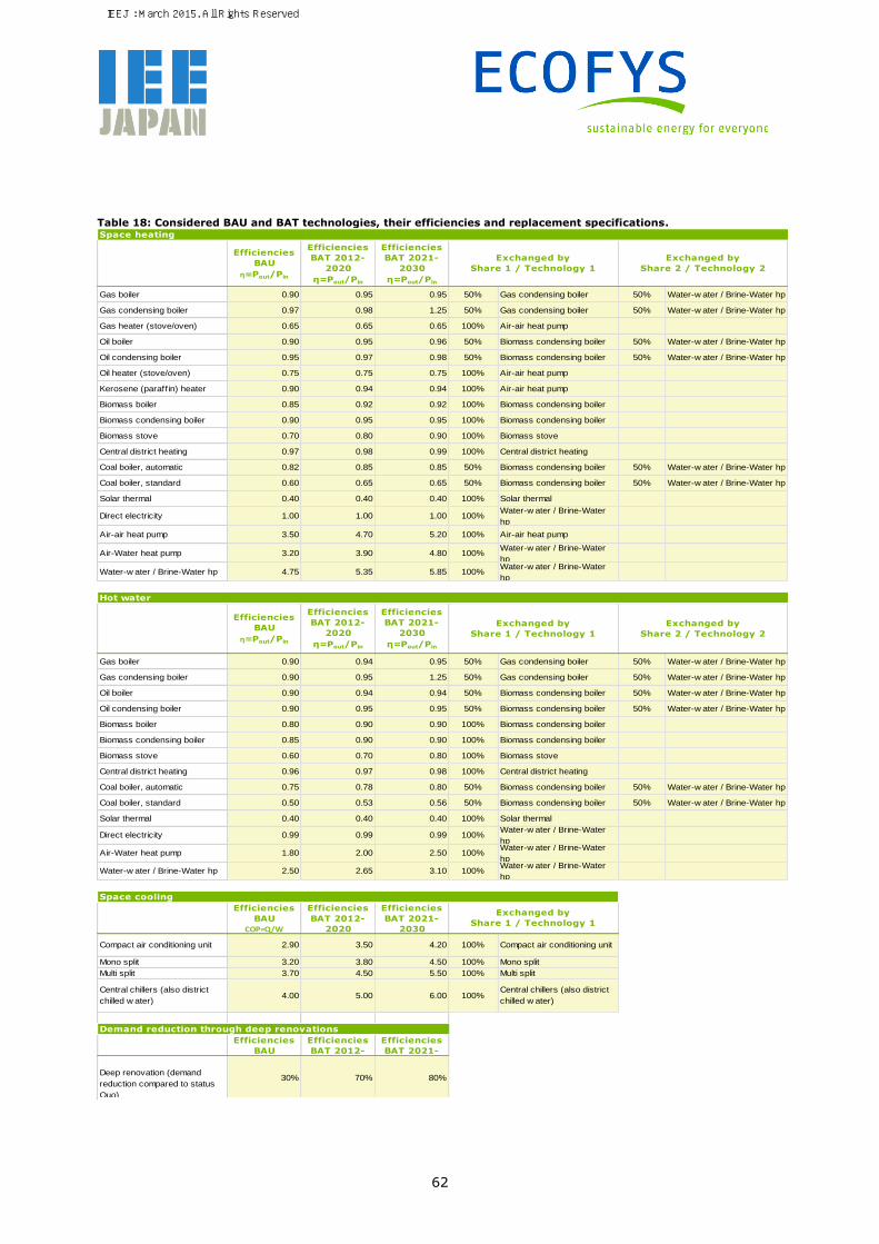
62

Table 18: Considered BAU and BAT technologies, their efficiencies and replacement specifications.

Efficiencies

BAU

η=Pout/Pin

Efficiencies

BAT 2012-

2020

η=Pout/Pin

Efficiencies

BAT 2021-

2030

η=Pout/Pin

Gas boiler 0.90 0.95 0.95 50% Gas condensing boiler 50% Water-w ater / Brine-Water hp

Gas condensing boiler 0.97 0.98 1.25 50% Gas condensing boiler 50% Water-w ater / Brine-Water hp

Gas heater (stove/oven) 0.65 0.65 0.65 100% Air-air heat pump

Oil boiler 0.90 0.95 0.96 50% Biomass condensing boiler 50% Water-w ater / Brine-Water hp

Oil condensing boiler 0.95 0.97 0.98 50% Biomass condensing boiler 50% Water-w ater / Brine-Water hp

Oil heater (stove/oven) 0.75 0.75 0.75 100% Air-air heat pump

Kerosene (paraff in) heater 0.90 0.94 0.94 100% Air-air heat pump

Biomass boiler 0.85 0.92 0.92 100% Biomass condensing boiler

Biomass condensing boiler 0.90 0.95 0.95 100% Biomass condensing boiler

Biomass stove 0.70 0.80 0.90 100% Biomass stove

Central district heating 0.97 0.98 0.99 100% Central district heating

Coal boiler, automatic 0.82 0.85 0.85 50% Biomass condensing boiler 50% Water-w ater / Brine-Water hp

Coal boiler, standard 0.60 0.65 0.65 50% Biomass condensing boiler 50% Water-w ater / Brine-Water hp

Solar thermal 0.40 0.40 0.40 100% Solar thermal

Direct electricity 1.00 1.00 1.00 100%Water-w ater / Brine-Water

hp

Air-air heat pump 3.50 4.70 5.20 100% Air-air heat pump

Air-Water heat pump 3.20 3.90 4.80 100%Water-w ater / Brine-Water

hp

Water-w ater / Brine-Water hp 4.75 5.35 5.85 100%Water-w ater / Brine-Water

hp

Hot water

Efficiencies

BAU

η=Pout/Pin

Efficiencies

BAT 2012-

2020

η=Pout/Pin

Efficiencies

BAT 2021-

2030

η=Pout/Pin

Gas boiler 0.90 0.94 0.95 50% Gas condensing boiler 50% Water-w ater / Brine-Water hp

Gas condensing boiler 0.90 0.95 1.25 50% Gas condensing boiler 50% Water-w ater / Brine-Water hp

Oil boiler 0.90 0.94 0.94 50% Biomass condensing boiler 50% Water-w ater / Brine-Water hp

Oil condensing boiler 0.90 0.95 0.95 50% Biomass condensing boiler 50% Water-w ater / Brine-Water hp

Biomass boiler 0.80 0.90 0.90 100% Biomass condensing boiler

Biomass condensing boiler 0.85 0.90 0.90 100% Biomass condensing boiler

Biomass stove 0.60 0.70 0.80 100% Biomass stove

Central district heating 0.96 0.97 0.98 100% Central district heating

Coal boiler, automatic 0.75 0.78 0.80 50% Biomass condensing boiler 50% Water-w ater / Brine-Water hp

Coal boiler, standard 0.50 0.53 0.56 50% Biomass condensing boiler 50% Water-w ater / Brine-Water hp

Solar thermal 0.40 0.40 0.40 100% Solar thermal

Direct electricity 0.99 0.99 0.99 100%Water-w ater / Brine-Water

hp

Air-Water heat pump 1.80 2.00 2.50 100%Water-w ater / Brine-Water

hp

Water-w ater / Brine-Water hp 2.50 2.65 3.10 100%Water-w ater / Brine-Water

hp

Space cooling

Efficiencies

BAU

COP=Q/W

Efficiencies

BAT 2012-

2020

Efficiencies

BAT 2021-

2030

Compact air conditioning unit 2.90 3.50 4.20 100% Compact air conditioning unit

Mono split 3.20 3.80 4.50 100% Mono split

Multi split 3.70 4.50 5.50 100% Multi split

Central chillers (also district

chilled w ater)4.00 5.00 6.00 100%

Central chillers (also district

chilled w ater)

Efficiencies

BAU

Efficiencies

BAT 2012-

Efficiencies

BAT 2021-

Deep renovation (demand

reduction compared to status

Quo)

30% 70% 80%

Space heating

Exchanged by

Share 1 / Technology 1

Exchanged by


Exchanged by


Exchanged by


Exchanged by


Demand reduction through deep renovations


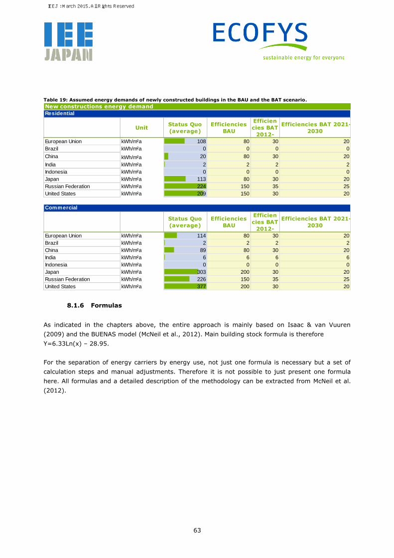
63

Table 19: Assumed energy demands of newly constructed buildings in the BAU and the BAT scenario.

8.1.6 Formulas

As indicated in the chapters above, the entire approach is mainly based on Isaac & van Vuuren

(2009) and the BUENAS model (McNeil et al., 2012). Main building stock formula is therefore

Y=6.33Ln(x) – 28.95.

For the separation of energy carriers by energy use, not just one formula is necessary but a set of

calculation steps and manual adjustments. Therefore it is not possible to just present one formula

here. All formulas and a detailed description of the methodology can be extracted from McNeil et al.

(2012).

UnitStatus Quo

(average)

Efficiencies

BAU

Efficien

cies BAT

2012-

Efficiencies BAT 2021-

2030

European Union kWh/m²a 108 80 30 20

Brazil kWh/m²a 0 0 0 0

China kWh/m²a 20 80 30 20

India kWh/m²a 2 2 2 2

Indonesia kWh/m²a 0 0 0 0

Japan kWh/m²a 113 80 30 20

Russian Federation kWh/m²a 224 150 35 25

United States kWh/m²a 209 150 30 20

Status Quo

(average)

Efficiencies

BAU

Efficien

cies BAT

2012-

Efficiencies BAT 2021-

2030

European Union kWh/m²a 114 80 30 20

Brazil kWh/m²a 2 2 2 2

China kWh/m²a 89 80 30 20

India kWh/m²a 6 6 6 6

Indonesia kWh/m²a 0 0 0 0

Japan kWh/m²a 303 200 30 20

Russian Federation kWh/m²a 226 150 35 25

United States kWh/m²a 377 200 30 20

New constructions energy demand

Residential

Commercial


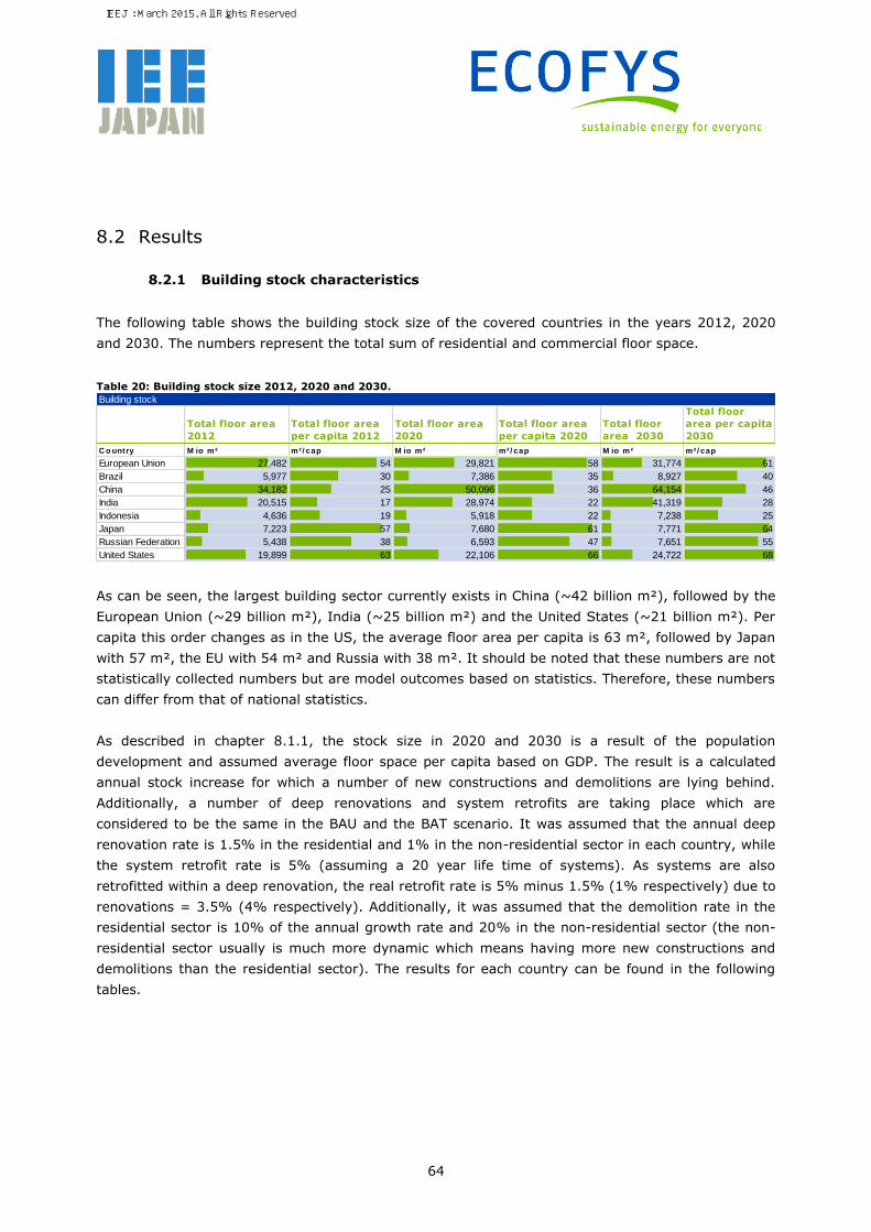
64

8.2 Results

8.2.1 Building stock characteristics

The following table shows the building stock size of the covered countries in the years 2012, 2020

and 2030. The numbers represent the total sum of residential and commercial floor space.

Table 20: Building stock size 2012, 2020 and 2030.

As can be seen, the largest building sector currently exists in China (~42 billion m²), followed by the

European Union (~29 billion m²), India (~25 billion m²) and the United States (~21 billion m²). Per

capita this order changes as in the US, the average floor area per capita is 63 m², followed by Japan

with 57 m², the EU with 54 m² and Russia with 38 m². It should be noted that these numbers are not

statistically collected numbers but are model outcomes based on statistics. Therefore, these numbers

can differ from that of national statistics.

As described in chapter 8.1.1, the stock size in 2020 and 2030 is a result of the population

development and assumed average floor space per capita based on GDP. The result is a calculated

annual stock increase for which a number of new constructions and demolitions are lying behind.

Additionally, a number of deep renovations and system retrofits are taking place which are

considered to be the same in the BAU and the BAT scenario. It was assumed that the annual deep

renovation rate is 1.5% in the residential and 1% in the non-residential sector in each country, while

the system retrofit rate is 5% (assuming a 20 year life time of systems). As systems are also

retrofitted within a deep renovation, the real retrofit rate is 5% minus 1.5% (1% respectively) due to

renovations = 3.5% (4% respectively). Additionally, it was assumed that the demolition rate in the

residential sector is 10% of the annual growth rate and 20% in the non-residential sector (the non-

residential sector usually is much more dynamic which means having more new constructions and

demolitions than the residential sector). The results for each country can be found in the following

tables.

Building stock

Total floor area

2012

Total floor area

per capita 2012

Total floor area

2020

Total floor area

per capita 2020

Total floor

area 2030

Total floor

area per capita

2030

C o untry M io m² m²/ cap M io m² m²/ cap M io m² m²/ cap

European Union 27,482 54 29,821 58 31,774 61

Brazil 5,977 30 7,386 35 8,927 40

China 34,182 25 50,096 36 64,154 46

India 20,515 17 28,974 22 41,319 28

Indonesia 4,636 19 5,918 22 7,238 25

Japan 7,223 57 7,680 61 7,771 64

Russian Federation 5,438 38 6,593 47 7,651 55

United States 19,899 63 22,106 66 24,722 68


65

Table 21: Building stock development 2012-2020.

Table 22: Building stock development 2020-2030.

8.2.2 Energy consumption / emissions (all energy uses) of the building stock

Table 23 shows the total and specific energy consumption as well as CO2 emissions in the building

sector of the eight covered countries in 2012. The numbers represent the entire energy

consumption / emissions in the sector which means that all types of energy uses are included (not

just space heating, hot water and space cooling).

Building stock development 2012-2020

Total floor

area 2012

Total number

of newly

constructed

floor area

2013-2020

Total number

of

demolished

floor area

2013-2020

Total number

of renovated

floor area

(incl. System

exchange)

2013-2020

Total number

of retrofitted

floor area

(system

exchange)

2013-2020

Total floor

area 2020

C o untry M io m² M io m² M io m² M io m² M io m² M io m²

European Union 27,482 2,663 -324 3,125 8,286 29,821

Brazil 5,977 1,590 -181 746 1,882 7,386

China 34,182 17,981 -2,066 4,622 11,605 50,096

India 20,515 9,436 -977 2,777 6,806 28,974

Indonesia 4,636 1,431 -149 599 1,470 5,918

Japan 7,223 522 -65 813 2,163 7,680

Russian Federation 5,438 1,318 -163 662 1,711 6,593

United States 19,899 2,495 -288 2,270 6,074 22,106

Building stock development 2020-2030

Total floor

area 2020

Total number

of newly

constructed

floor area

2021-2030

Total number

of

demolished

floor area

2021-2030

Total number

of renovated

floor area

(incl. System

exchange)

2021-2030

Total number

of retrofitted

floor area

(system

exchange)

2021-2030

Total floor

area 2030

C o untry M io m² M io m² M io m² M io m² M io m² M io m²

European Union 29,821 2,225 -272 4,196 11,179 31,774

Brazil 7,386 1,744 -203 1,134 2,897 8,927

China 50,096 16,015 -1,957 7,868 20,271 64,154

India 28,974 13,842 -1,497 4,906 12,161 41,319

Indonesia 5,918 1,477 -157 935 2,311 7,238

Japan 7,680 106 -15 1,054 2,815 7,771

Russian Federation 6,593 1,211 -153 976 2,566 7,651

United States 22,106 2,957 -340 3,164 8,475 24,722


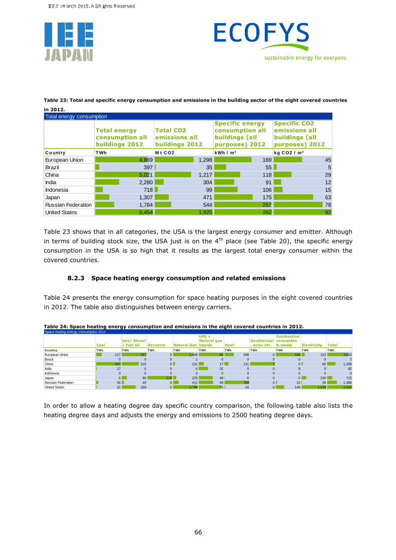
66

Table 23: Total and specific energy consumption and emissions in the building sector of the eight covered countries

in 2012.

Table 23 shows that in all categories, the USA is the largest energy consumer and emitter. Although

in terms of building stock size, the USA just is on the 4th place (see Table 20), the specific energy

consumption in the USA is so high that it results as the largest total energy consumer within the

covered countries.

8.2.3 Space heating energy consumption and related emissions

Table 24 presents the energy consumption for space heating purposes in the eight covered countries

in 2012. The table also distinguishes between energy carriers.

Table 24: Space heating energy consumption and emissions in the eight covered countries in 2012.

In order to allow a heating degree day specific country comparison, the following table also lists the

heating degree days and adjusts the energy and emissions to 2500 heating degree days.

Total energy consumption

Total energy

consumption all

buildings 2012

Total CO2

emissions all

buildings 2012

Specific energy

consumption all

buildings (all

purposes) 2012

Specific CO2

emissions all

buildings (all

purposes) 2012

C o untry T Wh M t C O2 kWh / m² kg C O2 / m²

European Union 4,869 1,298 169 45

Brazil 397 35 55 5

China 5,021 1,217 118 29

India 2,280 304 91 12

Indonesia 718 99 106 15

Japan 1,307 471 175 63

Russian Federation 1,784 544 257 78

United States 5,454 1,925 262 92

Space heating energy consumption 2012

Coal

Gas/ Diesel

/ fuel oil Kerosine Natural Gas

LPG +

Natural gas

liquids Heat

Geothermal

, solar etc

Combustion

renewable

& waste Electricity Total

C o untry T Wh T Wh T Wh T Wh T Wh T Wh T Wh T Wh T Wh T Wh

European Union 127 457 0 1,448 85 298 0 444 151 3,010

Brazil 0 0 0 1 0 0 0 0 0 2

China 553 316 0 131 17 131 0 0 60 1,208

India 17 0 0 6 32 0 0 8 0 62

Indonesia 0 0 0 0 0 0 0 0 0 0

Japan 6 90 110 225 48 6 0 0 230 715

Russian Federation 46 43 0 411 49 790 0 22 26 1,388

United States 15 259 0 1,784 75 16 0 149 1,238 3,536


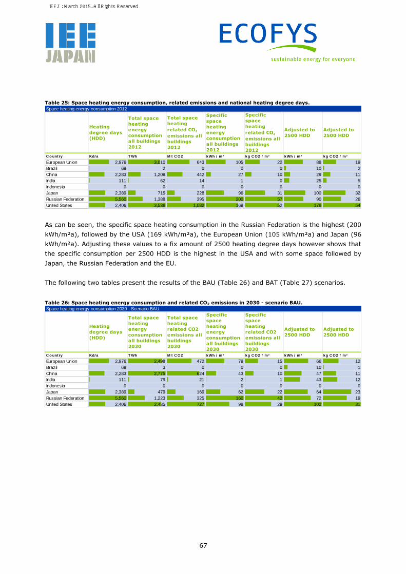
67

Table 25: Space heating energy consumption, related emissions and national heating degree days.

As can be seen, the specific space heating consumption in the Russian Federation is the highest (200

kWh/m²a), followed by the USA (169 kWh/m²a), the European Union (105 kWh/m²a) and Japan (96

kWh/m²a). Adjusting these values to a fix amount of 2500 heating degree days however shows that

the specific consumption per 2500 HDD is the highest in the USA and with some space followed by

Japan, the Russian Federation and the EU.

The following two tables present the results of the BAU (Table 26) and BAT (Table 27) scenarios.

Table 26: Space heating energy consumption and related CO2 emissions in 2030 - scenario BAU.

Space heating energy consumption 2012

Heating

degree days

(HDD)

Total space

heating

energy

consumption

all buildings

2012

Total space

heating

related CO2

emissions all

buildings

2012

Specific

space

heating

energy

consumption

all buildings

2012

Specific

space

heating

related CO2

emissions all

buildings

2012

Adjusted to

2500 HDD

Adjusted to

2500 HDD

C o untry Kd/ a T Wh M t C O2 kWh / m² kg C O2 / m² kWh / m² kg C O2 / m²

European Union 2,976 3,010 643 105 22 88 19

Brazil 69 2 0 0 0 10 2

China 2,283 1,208 442 27 10 29 11

India 111 62 14 1 0 25 5

Indonesia 0 0 0 0 0 0 0

Japan 2,389 715 228 96 31 100 32

Russian Federation 5,560 1,388 395 200 57 90 26

United States 2,406 3,536 1,082 169 52 176 54

Space heating energy consumption 2030 - Scenario BAU

Heating

degree days

(HDD)

Total space

heating

energy

consumption

all buildings

2030

Total space

heating

related CO2

emissions all

buildings

2030

Specific

space

heating

energy

consumption

all buildings

2030

Specific

space

heating

related CO2

emissions all

buildings

2030

Adjusted to

2500 HDD

Adjusted to

2500 HDD


European Union 2,976 2,498 472 79 15 66 12

Brazil 69 3 0 0 0 10 1

China 2,283 2,775 624 43 10 47 11

India 111 79 21 2 1 43 12

Indonesia 0 0 0 0 0 0 0

Japan 2,389 479 169 62 22 64 23

Russian Federation 5,560 1,223 325 160 42 72 19

United States 2,406 2,435 727 98 29 102 31


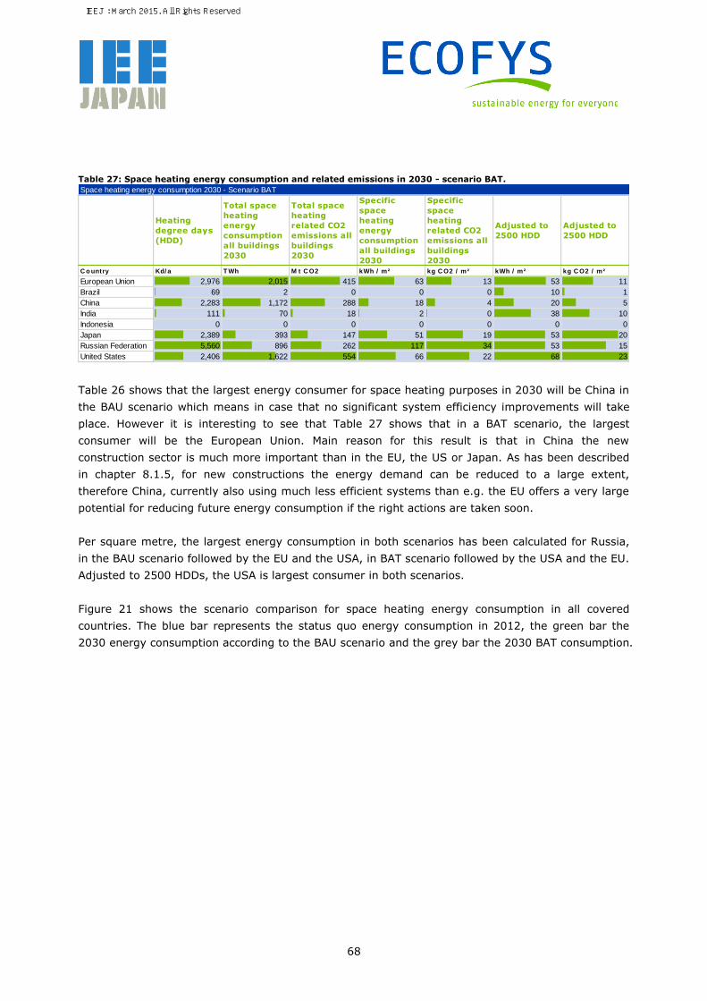
68

Table 27: Space heating energy consumption and related emissions in 2030 - scenario BAT.

Table 26 shows that the largest energy consumer for space heating purposes in 2030 will be China in

the BAU scenario which means in case that no significant system efficiency improvements will take

place. However it is interesting to see that Table 27 shows that in a BAT scenario, the largest

consumer will be the European Union. Main reason for this result is that in China the new

construction sector is much more important than in the EU, the US or Japan. As has been described

in chapter 8.1.5, for new constructions the energy demand can be reduced to a large extent,

therefore China, currently also using much less efficient systems than e.g. the EU offers a very large

potential for reducing future energy consumption if the right actions are taken soon.

Per square metre, the largest energy consumption in both scenarios has been calculated for Russia,

in the BAU scenario followed by the EU and the USA, in BAT scenario followed by the USA and the EU.

Adjusted to 2500 HDDs, the USA is largest consumer in both scenarios.

Figure 21 shows the scenario comparison for space heating energy consumption in all covered

countries. The blue bar represents the status quo energy consumption in 2012, the green bar the

2030 energy consumption according to the BAU scenario and the grey bar the 2030 BAT consumption.

Space heating energy consumption 2030 - Scenario BAT

Heating

degree days

(HDD)

Total space

heating

energy

consumption

all buildings

2030

Total space

heating

related CO2

emissions all

buildings

2030

Specific

space

heating

energy

consumption

all buildings

2030

Specific

space

heating

related CO2

emissions all

buildings

2030

Adjusted to

2500 HDD

Adjusted to

2500 HDD


European Union 2,976 2,015 415 63 13 53 11

Brazil 69 2 0 0 0 10 1

China 2,283 1,172 288 18 4 20 5

India 111 70 18 2 0 38 10

Indonesia 0 0 0 0 0 0 0

Japan 2,389 393 147 51 19 53 20

Russian Federation 5,560 896 262 117 34 53 15

United States 2,406 1,622 554 66 22 68 23


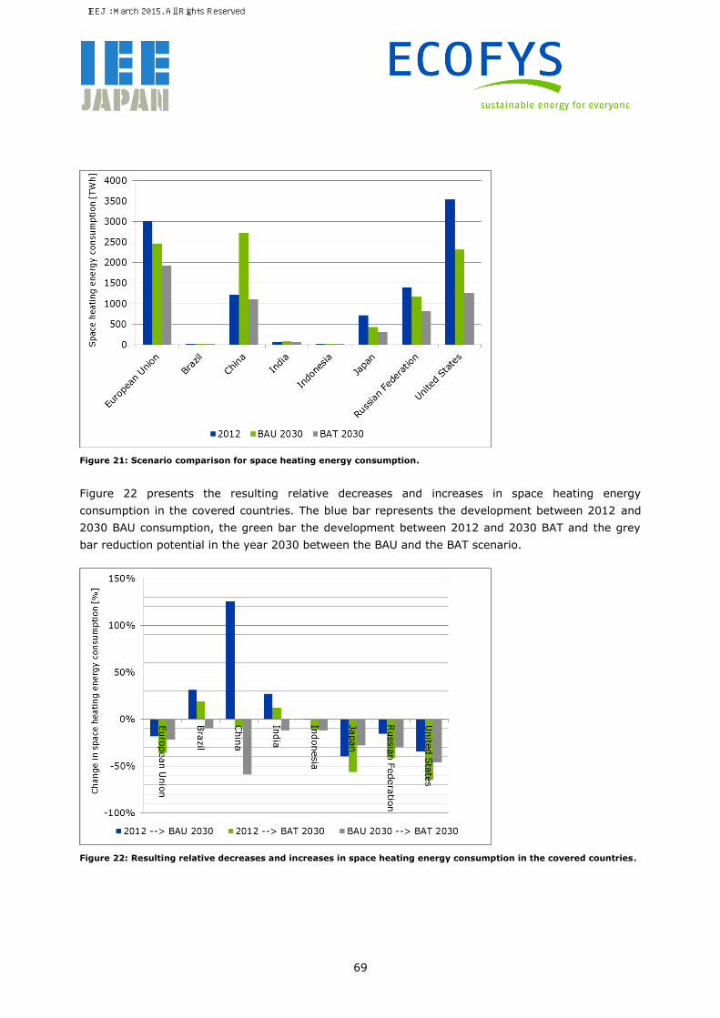
69

Figure 21: Scenario comparison for space heating energy consumption.

Figure 22 presents the resulting relative decreases and increases in space heating energy

consumption in the covered countries. The blue bar represents the development between 2012 and

2030 BAU consumption, the green bar the development between 2012 and 2030 BAT and the grey

bar reduction potential in the year 2030 between the BAU and the BAT scenario.

Figure 22: Resulting relative decreases and increases in space heating energy consumption in the covered countries.


70

The following Table 28 and Table 29 show the underlying numbers of the scenarios. Table 28 contains

the final energy data, Table 29 CO2 emission data.

Table 28: Scenario comparison of space heating energy consumption in the covered countries.

Table 29: Scenario comparison of space heating related CO2 emissions in the covered countries.

8.2.4 Hot water energy consumption and related emissions

Energy for hot water generation is an important energy use responsible for a large amount of

emissions in the covered countries. Table 30 shows the energy consumption for hot water generation

in the eight covered countries in 2012. The table also distinguishes between energy carriers.

Table 30: Hot water energy consumption and emissions in the eight covered countries in 2012.

Table 31 additionally presents the specific energy consumption per square metre in 2012 and the

related emissions from hot water generation in the covered countries.

2012 BAU 2030 BAT 20302012 --> BAU

2030

2012 -->

BAT 2030

BAU 2030 -->

BAT 2030

TWh TWh TWh % % %

European Union 3,010 2,459 1,927 -18% -36% -22%

Brazil 2 3 2 31% 19% -10%

China 1,208 2,721 1,108 125% -8% -59%

India 62 78 69 27% 12% -12%

Indonesia 0 0 0 1% -12% -12%

Japan 715 432 311 -40% -57% -28%

Russian Federation 1,388 1,169 821 -16% -41% -30%

United States 3,536 2,315 1,252 -35% -65% -46%

Space heating scenario comparison

2012 BAU 2030 BAT 20302012 --> BAU

2030

2012 -->

BAT 2030

BAU 2030 -->

BAT 2030

Mt CO2 Mt CO2 Mt CO2 % % %

European Union 643 438 365 -32% -43% -17%

Brazil 0 0 0 -50% -57% -15%

China 442 612 274 39% -38% -55%

India 14 21 17 48% 23% -17%

Indonesia 0 0 0 27% 4% -18%

Japan 228 157 125 -31% -45% -20%

Russian Federation 395 313 250 -21% -37% -20%

United States 1,082 700 479 -35% -56% -32%

Space heating scenario comparison

Hot w ater energy consumption 2012

Coal

Gas/ Diesel

/ fuel oil Kerosine Natural Gas

LPG +

Natural gas

liquids Heat

Geothermal

, solar etc

Combustion

renewable

& waste Electricity Total

C o untry T Wh T Wh T Wh T Wh T Wh T Wh T Wh T Wh T Wh T Wh

European Union 0 50 0 171 10 36 29 0 130 426

Brazil 0 0 0 4 12 0 0 2 25 43

China 0 53 0 63 0 82 37 0 44 278

India 23 0 0 13 70 0 0 30 4 140

Indonesia 0 8 0 2 45 0 0 2 0 58

Japan 0 0 0 85 39 0 6 0 56 186

Russian Federation 0 1 0 29 3 48 0 0 0 81

United States 0 31 0 271 28 0 18 0 149 497


71

Table 31: Hot water energy consumption and emissions in the eight covered countries in 2012.

According to our calculations, the highest specific energy consumption for hot water generation exists

in Japan (26 kWh/m²a) slightly followed by the USA (25 kWh/m²a). The EU and Russian Federation

can be classified as medium-range consumers (15/16 kWh/m²a), the other countries as low-range

consumers (7-8 kWh/m²a).

For the BAU and the BAT scenario we did not consider any demand reductions but considered a stable

specific energy demand for hot water generation between 2012 and 2030. The results of the BAU and

the BAT scenario can be found in Table 32 and Table 33.

Table 32: Hot water energy consumption and emissions in the eight covered countries in 2030 - Scenario BAU.

Hot water energy consumption 2012

Total hot water

energy

consumption all

buildings 2012

Total hot water

related CO2

emissions all

buildings 2012

Specific hot water

energy

consumption all

buildings 2012

Total hot water

related CO2

emissions all

buildings 2012

Country TWh Mt CO2 kWh / m² kg CO2 / m²

European Union 426 114 16 4

Brazil 43 5 7 1

China 278 119 8 3

India 140 30 7 1

Indonesia 58 13 13 3

Japan 186 54 26 7

Russian Federation 81 23 15 4

United States 497 144 25 7

Hot water energy consumption 2030 - Scenario BAU

Total hot water

energy

consumption all

buildings 2030

Total hot water

related CO2

emissions all

buildings 2030

Total hot water

energy

consumption all

buildings 2030

Total hot water

related CO2

emissions all

buildings 2030



Brazil 50 5 6 1

China 505 157 8 2

India 239 79 6 2

Indonesia 74 22 10 3

Japan 144 42 19 5




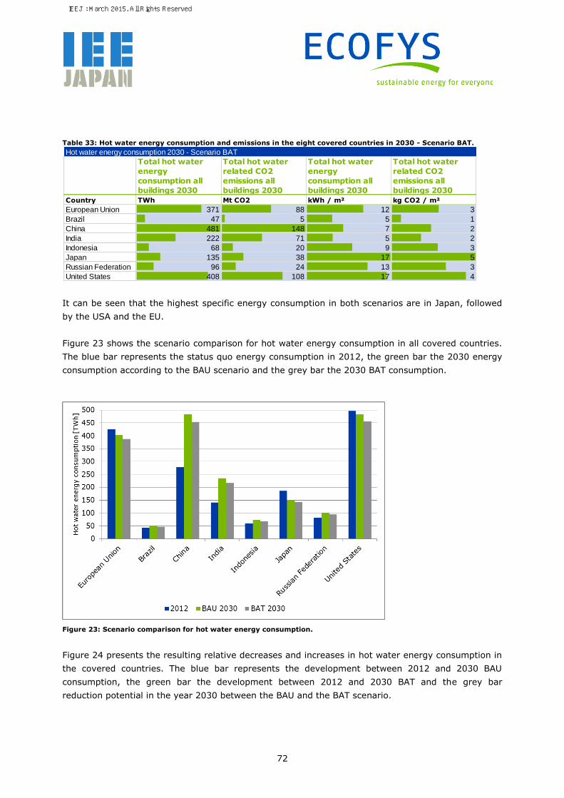
72

Table 33: Hot water energy consumption and emissions in the eight covered countries in 2030 - Scenario BAT.

It can be seen that the highest specific energy consumption in both scenarios are in Japan, followed

by the USA and the EU.

Figure 23 shows the scenario comparison for hot water energy consumption in all covered countries.

The blue bar represents the status quo energy consumption in 2012, the green bar the 2030 energy

consumption according to the BAU scenario and the grey bar the 2030 BAT consumption.

Figure 23: Scenario comparison for hot water energy consumption.

Figure 24 presents the resulting relative decreases and increases in hot water energy consumption in

the covered countries. The blue bar represents the development between 2012 and 2030 BAU

consumption, the green bar the development between 2012 and 2030 BAT and the grey bar

reduction potential in the year 2030 between the BAU and the BAT scenario.

Hot water energy consumption 2030 - Scenario BAT

Total hot water

energy

consumption all

buildings 2030

Total hot water

related CO2

emissions all

buildings 2030

Total hot water

energy

consumption all

buildings 2030

Total hot water

related CO2

emissions all

buildings 2030



Brazil 47 5 5 1

China 481 148 7 2

India 222 71 5 2

Indonesia 68 20 9 3

Japan 135 38 17 5




73

Figure 24: Resulting relative decreases and increases in hot water energy consumption in the covered countries.

The following Table 34 and Table 35 and show the underlying numbers of the scenarios. Table 34

contains the final energy data, Table 35 the CO2 emission data.

Table 34: Scenario comparison of hot water energy consumption in the covered countries.

Table 35: Scenario comparison of hot water related CO2 emissions in the covered countries.

2012 BAU 2030 BAT 20302012 --> BAU

2030

2012 -->

BAT 2030

BAU 2030 -->

BAT 2030

TWh TWh TWh % % %

European Union 426 404 387 -5% -9% -4%

Brazil 43 50 47 16% 8% -7%

China 278 483 453 73% 63% -6%

India 140 235 217 68% 55% -8%

Indonesia 58 73 68 26% 16% -7%

Japan 186 151 142 -19% -23% -6%

Russian Federation 81 99 94 22% 16% -5%

United States 497 483 457 -3% -8% -5%

Hot water scenario comparison

2012 BAU 2030 BAT 20302012 --> BAU

2030

2012 -->

BAT 2030

BAU 2030 -->

BAT 2030


European Union 114 93 89 -18% -22% -5%

Brazil 5 5 4 -6% -15% -9%

China 119 151 139 27% 17% -8%

India 30 79 70 162% 133% -11%

Indonesia 13 22 20 69% 52% -10%

Japan 54 43 40 -20% -25% -7%


United States 144 126 118 -12% -18% -6%

Hot water scenario comparison


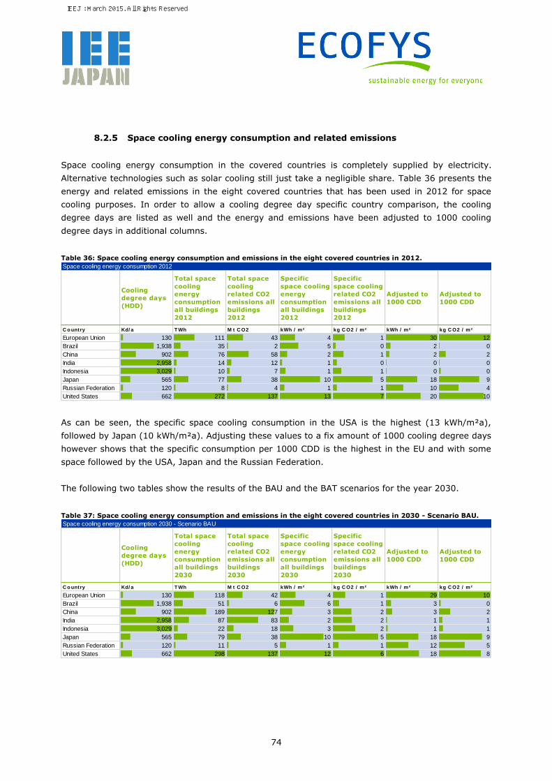
74

8.2.5 Space cooling energy consumption and related emissions

Space cooling energy consumption in the covered countries is completely supplied by electricity.

Alternative technologies such as solar cooling still just take a negligible share. Table 36 presents the

energy and related emissions in the eight covered countries that has been used in 2012 for space

cooling purposes. In order to allow a cooling degree day specific country comparison, the cooling

degree days are listed as well and the energy and emissions have been adjusted to 1000 cooling

degree days in additional columns.

Table 36: Space cooling energy consumption and emissions in the eight covered countries in 2012.

As can be seen, the specific space cooling consumption in the USA is the highest (13 kWh/m²a),

followed by Japan (10 kWh/m²a). Adjusting these values to a fix amount of 1000 cooling degree days

however shows that the specific consumption per 1000 CDD is the highest in the EU and with some

space followed by the USA, Japan and the Russian Federation.

The following two tables show the results of the BAU and the BAT scenarios for the year 2030.

Table 37: Space cooling energy consumption and emissions in the eight covered countries in 2030 - Scenario BAU.

Space cooling energy consumption 2012

Cooling

degree days

(HDD)

Total space

cooling

energy

consumption

all buildings

2012

Total space

cooling

related CO2

emissions all

buildings

2012

Specific

space cooling

energy

consumption

all buildings

2012

Specific

space cooling

related CO2

emissions all

buildings

2012

Adjusted to

1000 CDD

Adjusted to

1000 CDD


European Union 130 111 43 4 1 30 12

Brazil 1,938 35 2 5 0 2 0

China 902 76 58 2 1 2 2

India 2,958 14 12 1 0 0 0

Indonesia 3,029 10 7 1 1 0 0

Japan 565 77 38 10 5 18 9

Russian Federation 120 8 4 1 1 10 4

United States 662 272 137 13 7 20 10

Space cooling energy consumption 2030 - Scenario BAU

Cooling

degree days

(HDD)

Total space

cooling

energy

consumption

all buildings

2030

Total space

cooling

related CO2

emissions all

buildings

2030

Specific

space cooling

energy

consumption

all buildings

2030

Specific

space cooling

related CO2

emissions all

buildings

2030

Adjusted to

1000 CDD

Adjusted to

1000 CDD


European Union 130 118 42 4 1 29 10

Brazil 1,938 51 6 6 1 3 0

China 902 189 127 3 2 3 2

India 2,958 87 83 2 2 1 1

Indonesia 3,029 22 18 3 2 1 1

Japan 565 79 38 10 5 18 9


United States 662 298 137 12 6 18 8


75

Table 38: Space cooling energy consumption and emissions in the eight covered countries in 2030 - Scenario BAT.

It can be seen that the main outcomes keep the same. Largest total and specific energy consumer in

both scenarios is the USA, adjusting the consumption to 1000 CDD shows that the EU will still be tha

largest consumer in 2030.

Figure 25 shows the scenario comparison for space cooling energy consumption in all covered

countries. The blue bar represents the status quo energy consumption in 2012, the green bar the

2030 energy consumption according to the BAU scenario and the grey bar the 2030 BAT consumption.

Figure 25: Scenario comparison for space cooling energy consumption.

Figure 26 presents the resulting relative decreases and increases in space cooling energy

consumption in the covered countries. The blue bar represents the development between 2012 and

2030 BAU consumption, the green bar the development between 2012 and 2030 BAT and the grey

bar reduction potential in the year 2030 between the BAU and the BAT scenario.

Space cooling energy consumption 2030 - Scenario BAT

Cooling

degree days

(HDD)

Total space

cooling

energy

consumption

all buildings

2030

Total space

cooling

related CO2

emissions all

buildings

2030

Specific

space cooling

energy

consumption

all buildings

2030

Specific

space cooling

related CO2

emissions all

buildings

2030

Adjusted to

1000 CDD

Adjusted to

1000 CDD


European Union 130 115 41 4 1 28 10

Brazil 1,938 45 5 5 1 3 0

China 902 153 103 2 2 3 2

India 2,958 67 64 2 2 1 1

Indonesia 3,029 19 15 3 2 1 1

Japan 565 78 37 10 5 18 9


United States 662 288 132 12 5 18 8


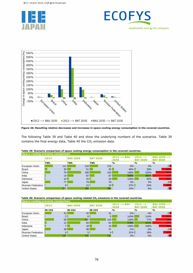
76

Figure 26: Resulting relative decreases and increases in space cooling energy consumption in the covered countries.

The following Table 39 and Table 40 and show the underlying numbers of the scenarios. Table 39

contains the final energy data, Table 40 the CO2 emission data.

Table 39: Scenario comparison of space cooling energy consumption in the covered countries.

Table 40: Scenario comparison of space cooling related CO2 emssions in the covered countries.

2012 BAU 2030 BAT 20302012 --> BAU

2030

2012 -->

BAT 2030

BAU 2030 -->

BAT 2030

TWh TWh TWh % % %

European Union 111 118 115 6% 4% -2%

Brazil 35 51 45 46% 29% -12%

China 76 189 153 148% 102% -19%

India 14 87 67 506% 366% -23%

Indonesia 10 22 19 126% 92% -15%

Japan 77 79 78 3% 2% -1%


United States 272 298 288 10% 6% -3%

Space cooling scenario comparison

2012 BAU 2030 BAT 20302012 --> BAU

2030

2012 -->

BAT 2030

BAU 2030 -->

BAT 2030


European Union 43 42 41 -2% -4% -2%

Brazil 2 6 5 143% 114% -12%

China 58 127 103 118% 77% -19%

India 12 83 64 578% 421% -23%

Indonesia 7 18 15 136% 100% -15%

Japan 38 38 37 -1% -2% -1%


United States 137 137 132 0% -3% -3%

Space cooling scenario comparison


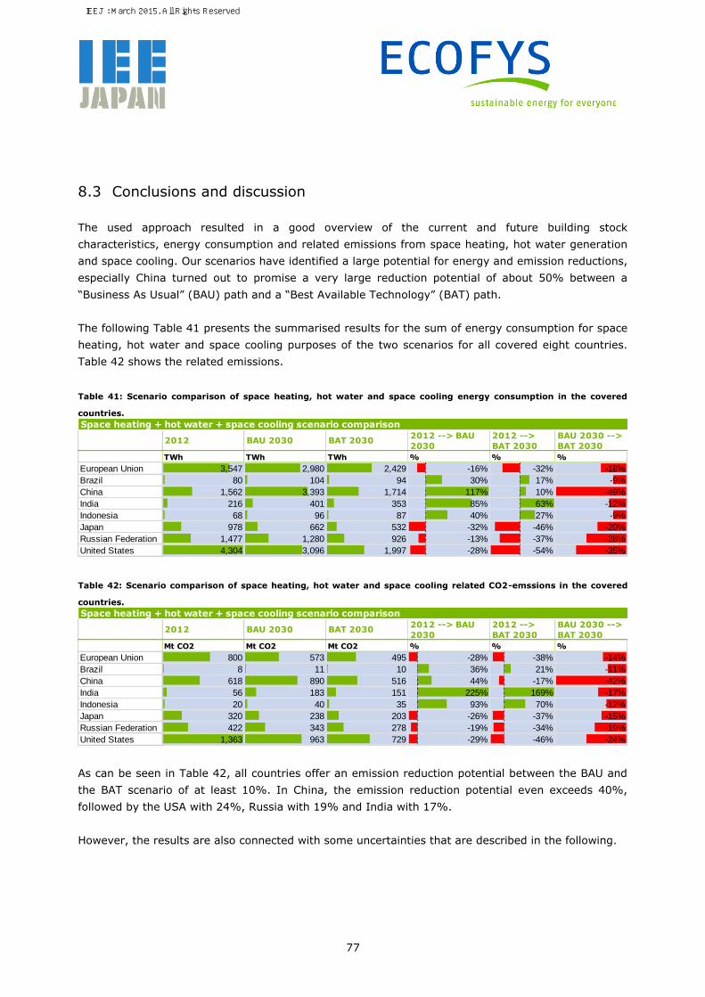
77

8.3 Conclusions and discussion

The used approach resulted in a good overview of the current and future building stock

characteristics, energy consumption and related emissions from space heating, hot water generation

and space cooling. Our scenarios have identified a large potential for energy and emission reductions,

especially China turned out to promise a very large reduction potential of about 50% between a

“Business As Usual” (BAU) path and a “Best Available Technology” (BAT) path.

The following Table 41 presents the summarised results for the sum of energy consumption for space

heating, hot water and space cooling purposes of the two scenarios for all covered eight countries.

Table 42 shows the related emissions.

Table 41: Scenario comparison of space heating, hot water and space cooling energy consumption in the covered

countries.

Table 42: Scenario comparison of space heating, hot water and space cooling related CO2-emssions in the covered

countries.

As can be seen in Table 42, all countries offer an emission reduction potential between the BAU and

the BAT scenario of at least 10%. In China, the emission reduction potential even exceeds 40%,

followed by the USA with 24%, Russia with 19% and India with 17%.

However, the results are also connected with some uncertainties that are described in the following.

2012 BAU 2030 BAT 20302012 --> BAU

2030

2012 -->

BAT 2030

BAU 2030 -->

BAT 2030

TWh TWh TWh % % %

European Union 3,547 2,980 2,429 -16% -32% -18%

Brazil 80 104 94 30% 17% -9%

China 1,562 3,393 1,714 117% 10% -49%

India 216 401 353 85% 63% -12%

Indonesia 68 96 87 40% 27% -9%

Japan 978 662 532 -32% -46% -20%

Russian Federation 1,477 1,280 926 -13% -37% -28%

United States 4,304 3,096 1,997 -28% -54% -35%

Space heating + hot water + space cooling scenario comparison

2012 BAU 2030 BAT 20302012 --> BAU

2030

2012 -->

BAT 2030

BAU 2030 -->

BAT 2030


European Union 800 573 495 -28% -38% -14%

Brazil 8 11 10 36% 21% -11%

China 618 890 516 44% -17% -42%

India 56 183 151 225% 169% -17%

Indonesia 20 40 35 93% 70% -12%

Japan 320 238 203 -26% -37% -15%

Russian Federation 422 343 278 -19% -34% -19%

United States 1,363 963 729 -29% -46% -24%

Space heating + hot water + space cooling scenario comparison


78

IEA statistics are strongly discussed in the international community as they often seem to be fuzzy in

some areas. However, advantage of IEA statistics is that they are available for almost all countries in

the world, collected and prepared with the same methodology, therefore streamlined and promising

the highest grade of accuracy. It should be noted that the total amount of consumed energy in a

country as reported by the IEA has a significant impact on the specific energy consumption values

that are calculated based on it.

The building stock data used for this analysis is based on general correlations and therefore definitely

holds a specific risk for uncertainty. However this approach promises a good grade of consistency as

in national statistics it is often unclear e.g. which kinds of buildings are included in a specific statistic

and which not. Additionally the definitions for living area, useful area etc. normally vary from country

to country. Using this approach assumes the same definitions and correlations and therefore is

assumed to be appropriate for this kind of analysis. It should be noted that also the size of the

building stock has a significant impact on the specific energy consumption values.

The entire methodology for splitting the total energy consumption in the countries into the different

energy uses holds a large number of uncertainties. However we assume that the numbers give a

good indication about the relative share of energy that is used for different energy uses within one

country. And assuming that IEA data is reliable, also a cross country comparison should be relatively

secure.


79

References

IEA, 2013. Energy balances for OECD and non-OECD countries - 2013. International Energy Agency,

Paris, France.

IPCC, 2006. 2006 IPCC Guidelines for National Greenhouse Gas Inventories, Volume 2: Energy.

Hayama, Japan.

McNeil, M.A., Letschert, V.E., Can, S. de la R. du, Ke, J., 2012. Bottom-Up Energy Analysis System –

Methodology and Results. Online Publication.

Isaac, M., van Vuuren, D.P., 2009. Modeling global residential sector energy demand for heating and

air conditioning in the context of climate change. Energy Policy 37, 507–521.

Schimschar, S., 2008. PhD Thesis: Energy- und emission reductions in the global building stock.

University of Utrecht, Netherlands.



ECOFYS Germany GmbH

Am Wassermann 36

50829 Cologne

T: +49 (0) 221 27070-100

F: +49 (0) 221 27070-011

E: [email protected]

I: www.ecofys.com

Institute of Energy Economics, Japan

13-1, Kachidoki 1-chome, Chuo-ku

104-0054 Tokyo

T: +81 (3) 5547 0231

F: +81 (3) 5547 0227

I: eneken.ieej.or.jp


Contact：[email protected]