6th International Conference on Earthquake Geotechnical Engineering 1-4 November 2015 Christchurch, New Zealand

Development of Realistic Vs Profiles in Christchurch, New Zealand via Active and

Ambient Surface Wave Data: Methodologies for Inversion in Complex Inter-bedded Geology

D.P. Teague 1, B.R. Cox 2, B.A. Bradley 3, L.M. Wotherspoon 4

ABSTRACT

Deep shear wave velocity (Vs) profiles (>400 m) were developed at 14 sites throughout

Christchurch, New Zealand using surface wave methods. This paper focuses on the inversion of surface wave data collected at one of these sites, Hagley Park. This site is located on the deep soils of the Canterbury Plains, which consist of alluvial gravels inter-bedded with estuarine and marine sands, silts, clays and peats. Consequently, significant velocity contrasts exist at the interface between geologic formations. In order to develop realistic velocity models in this complex geologic environment, a-priori geotechnical and geologic data were used to identify the boundaries between geologic formations. This information aided in developing the layering for the inversion parameters. Moreover, empirical reference Vs profiles based on material type and confining pressure were used to develop realistic Vs ranges for each layer. Both the a-priori layering information and the reference Vs curves proved to be instrumental in generating realistic velocity models that account for the complex inter-bedded geology in the Canterbury Plains.

Introduction

Deep shear wave velocity (Vs) profiles have been developed at 14 sites throughout Christchurch, New Zealand (refer to Figure 1a) using a combination of active-source and ambient-wavefield surface wave testing. Because of the complex geology in Christchurch (Brown et al. 1988), the use of surface wave methods to develop Vs profiles presents several challenges. This paper will primarily focus on the inversion of surface wave data collected at the Hagley Park site as a means to illustrate challenges and methodologies used to develop reliable deep Vs profiles at all testing locations. These Vs profiles play a key role in the ongoing development of a high-resolution velocity model of the Canterbury Basin (Lee et al. 2014). Hagley Park is approximately 10.5 km west of the eastern coast of Pegasus Bay on the South Island of New Zealand, on the western edge of the Christchurch Central Business District. Like the majority of the 14 test sites, Hagley Park is located on the deep alluvial soils of the Canterbury Plains. The near-surface geology (approximately top 20-40 m) of the Canterbury Plains is comprised of the Springston and Christchurch Formations (refer to Figure 2). The Springston Formation consists of Holocene alluvial sands and gravels with occasional silt and clay lenses. The Christchurch formation consists of Holocene estuarine, lagoon, dune and coastal swamp deposits of gravel, sand, silt, clay and peat. Beneath the Christchurch formation, alluvial gravels inter-bed with estuarine and marine sands, silts, clays and peats (Brown et al. 1988).

1University of Texas, Graduate Student, Dept. of Civil, Arch. and Envir. Eng., Austin, TX, USA, dteague@utexas.edu 2University of Texas, Associate Professor, Dept. of Civil, Arch. and Envir. Eng., Austin, TX, USA, brcox@utexas.edu 3University of Canterbury, Associate Professor, Dept. of Civil and Nat. Res. Eng., Christchurch, NZ, brendon.bradley@canterbury.ac.nz 4University of Auckland, EQC Research Fellow, Dept. of Civil and Environmental Eng., Auckland, NZ, l.wotherspoon@auckland.ac.nz

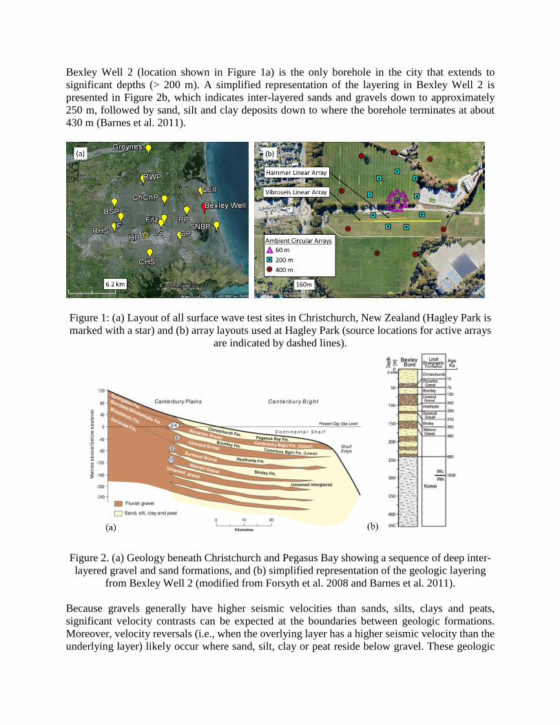
Bexley Well 2 (location shown in Figure 1a) is the only borehole in the city that extends to significant depths (> 200 m). A simplified representation of the layering in Bexley Well 2 is presented in Figure 2b, which indicates inter-layered sands and gravels down to approximately 250 m, followed by sand, silt and clay deposits down to where the borehole terminates at about 430 m (Barnes et al. 2011).

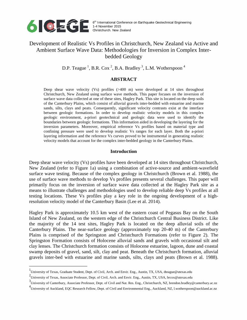
Figure 1: (a) Layout of all surface wave test sites in Christchurch, New Zealand (Hagley Park is marked with a star) and (b) array layouts used at Hagley Park (source locations for active arrays

are indicated by dashed lines).

Figure 2. (a) Geology beneath Christchurch and Pegasus Bay showing a sequence of deep inter-layered gravel and sand formations, and (b) simplified representation of the geologic layering

from Bexley Well 2 (modified from Forsyth et al. 2008 and Barnes et al. 2011). Because gravels generally have higher seismic velocities than sands, silts, clays and peats, significant velocity contrasts can be expected at the boundaries between geologic formations. Moreover, velocity reversals (i.e., when the overlying layer has a higher seismic velocity than the underlying layer) likely occur where sand, silt, clay or peat reside below gravel. These geologic

conditions present several challenges for surface wave methods. First, when strong velocity contrasts and velocity reversals are present, the fundamental mode of surface wave propagation may not be dominant over certain frequency bands. Therefore, the experimental dispersion data may contain significant higher-mode energy, which can be challenging to invert accurately. Additionally, defining an inversion parameter space that will yield accurate Vs profiles for such complex geologic conditions is not trivial. Initial inversion parameters such as the number of layers and ranges for their corresponding thicknesses, shear wave velocities (Vs), and compression wave velocities (Vp) must be chosen carefully. The parameter space must be sufficiently broad to capture the complex geology, yet adequately constrained to prevent the inversion routine from pursuing unrealistic ground models. An accurate determination of the proper number of layers can only be determined with the aid of a-priori geologic or borehole information. The sensor arrays used to obtain surface wave data at Hagley Park are shown in Figure 1b. The following data were acquired at the site: (a) active-source (sledgehammer) records from 48, 4.5-Hz vertical geophones spaced at 2 m and collected using source offsets of 5, 10, 20 and 40 m, (b) active-source (vibroseis) records from 24, 1-Hz vertical geophones spaced at 10 m and collected using source offsets of 20, 40 and 80 m, and (c) ambient-wavefield records from 10 broadband, 3-component seismometers placed in circular arrays with diameters of 60, 200 and 400 m. The active-source and ambient-wavefield testing procedures were essentially the same for all sites, and are described in detail in Cox et al. (2014).

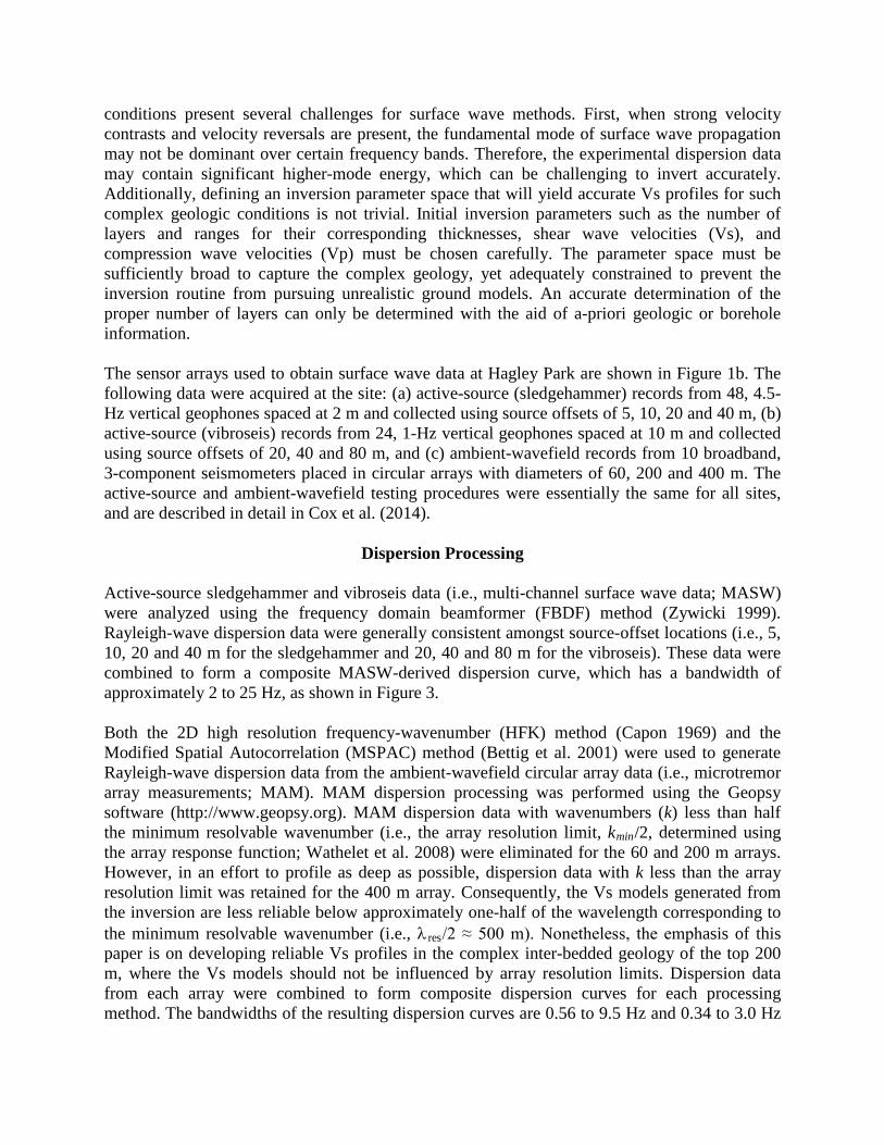
Dispersion Processing Active-source sledgehammer and vibroseis data (i.e., multi-channel surface wave data; MASW) were analyzed using the frequency domain beamformer (FBDF) method (Zywicki 1999). Rayleigh-wave dispersion data were generally consistent amongst source-offset locations (i.e., 5, 10, 20 and 40 m for the sledgehammer and 20, 40 and 80 m for the vibroseis). These data were combined to form a composite MASW-derived dispersion curve, which has a bandwidth of approximately 2 to 25 Hz, as shown in Figure 3.

Both the 2D high resolution frequency-wavenumber (HFK) method (Capon 1969) and the Modified Spatial Autocorrelation (MSPAC) method (Bettig et al. 2001) were used to generate Rayleigh-wave dispersion data from the ambient-wavefield circular array data (i.e., microtremor array measurements; MAM). MAM dispersion processing was performed using the Geopsy software (http://www.geopsy.org). MAM dispersion data with wavenumbers (k) less than half the minimum resolvable wavenumber (i.e., the array resolution limit, kmin/2, determined using the array response function; Wathelet et al. 2008) were eliminated for the 60 and 200 m arrays. However, in an effort to profile as deep as possible, dispersion data with k less than the array resolution limit was retained for the 400 m array. Consequently, the Vs models generated from the inversion are less reliable below approximately one-half of the wavelength corresponding to the minimum resolvable wavenumber (i.e., λres/2 ≈ 500 m). Nonetheless, the emphasis of this paper is on developing reliable Vs profiles in the complex inter-bedded geology of the top 200 m, where the Vs models should not be influenced by array resolution limits. Dispersion data from each array were combined to form composite dispersion curves for each processing method. The bandwidths of the resulting dispersion curves are 0.56 to 9.5 Hz and 0.34 to 3.0 Hz

for the HFK and MSPAC methods, respectively (refer to Figure 3). Further details regarding the dispersion processing for the MASW and MAM data can be found in Wood et al. (2014). HFK and MSPAC dispersion data are in good agreement at frequencies greater than 2 Hz and between 0.6-1.0 Hz. Moreover, this data agrees very well with the active-source data. However, the trend of the HFK and MSPAC dispersion data abruptly flattens/decreases between approximately 1 and 2 Hz. This discontinuity indicates that the dispersion data is likely transitioning from a higher Rayleigh-wave mode to a lower mode. Furthermore, the HFK data is biased towards higher phase velocities than the MSPAC data at frequencies less than 0.6 Hz.

Figure 3. Comparison of Rayleigh wave dispersion data at Hagley Park

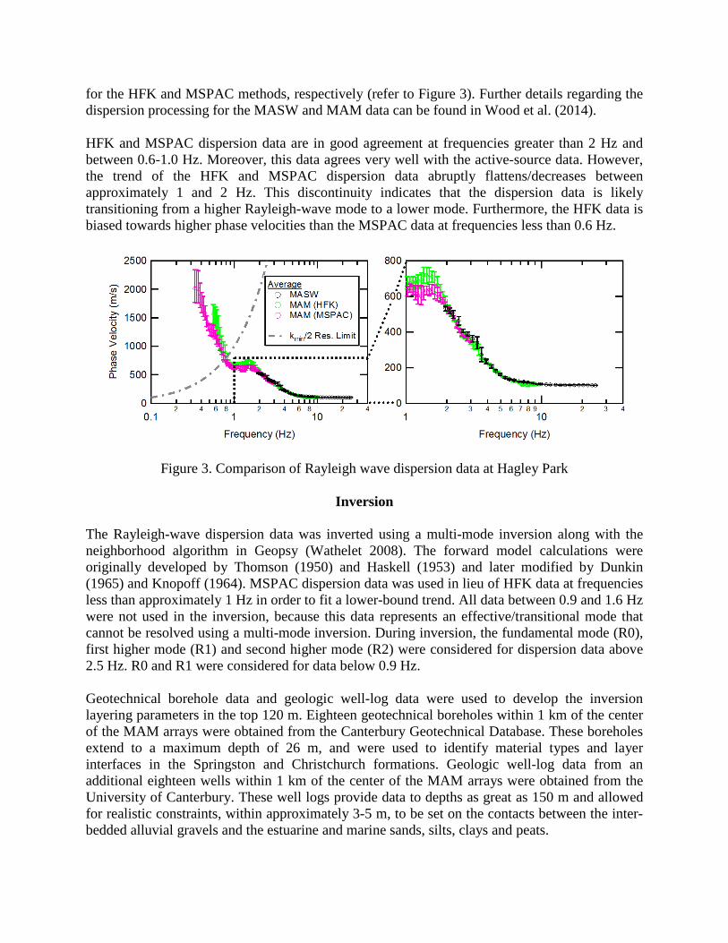
Inversion The Rayleigh-wave dispersion data was inverted using a multi-mode inversion along with the neighborhood algorithm in Geopsy (Wathelet 2008). The forward model calculations were originally developed by Thomson (1950) and Haskell (1953) and later modified by Dunkin (1965) and Knopoff (1964). MSPAC dispersion data was used in lieu of HFK data at frequencies less than approximately 1 Hz in order to fit a lower-bound trend. All data between 0.9 and 1.6 Hz were not used in the inversion, because this data represents an effective/transitional mode that cannot be resolved using a multi-mode inversion. During inversion, the fundamental mode (R0), first higher mode (R1) and second higher mode (R2) were considered for dispersion data above 2.5 Hz. R0 and R1 were considered for data below 0.9 Hz. Geotechnical borehole data and geologic well-log data were used to develop the inversion layering parameters in the top 120 m. Eighteen geotechnical boreholes within 1 km of the center of the MAM arrays were obtained from the Canterbury Geotechnical Database. These boreholes extend to a maximum depth of 26 m, and were used to identify material types and layer interfaces in the Springston and Christchurch formations. Geologic well-log data from an additional eighteen wells within 1 km of the center of the MAM arrays were obtained from the University of Canterbury. These well logs provide data to depths as great as 150 m and allowed for realistic constraints, within approximately 3-5 m, to be set on the contacts between the inter-bedded alluvial gravels and the estuarine and marine sands, silts, clays and peats.

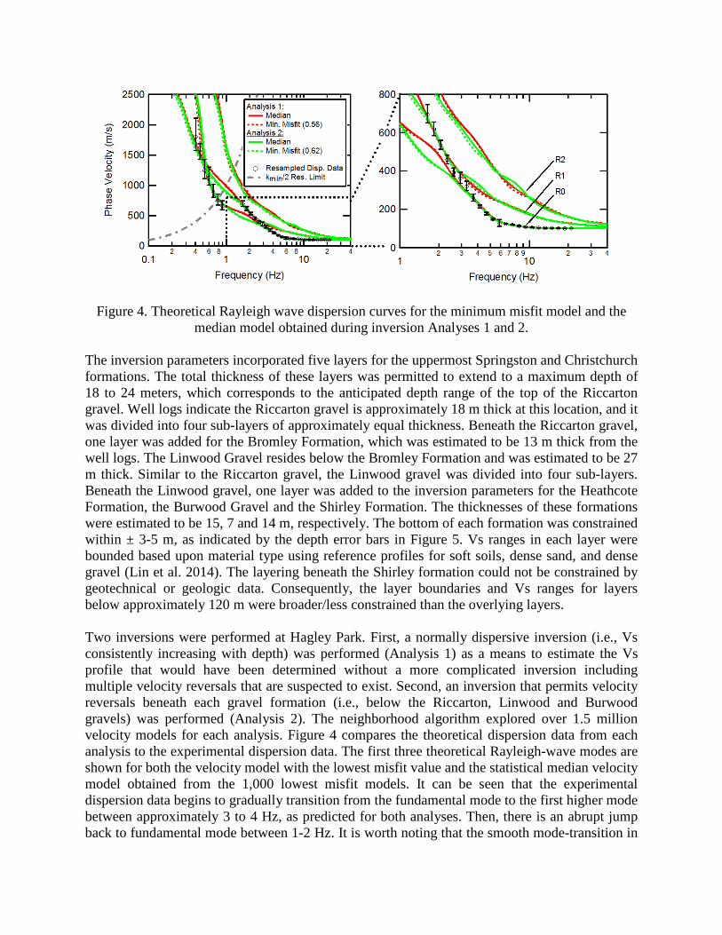
Figure 4. Theoretical Rayleigh wave dispersion curves for the minimum misfit model and the median model obtained during inversion Analyses 1 and 2.

The inversion parameters incorporated five layers for the uppermost Springston and Christchurch formations. The total thickness of these layers was permitted to extend to a maximum depth of 18 to 24 meters, which corresponds to the anticipated depth range of the top of the Riccarton gravel. Well logs indicate the Riccarton gravel is approximately 18 m thick at this location, and it was divided into four sub-layers of approximately equal thickness. Beneath the Riccarton gravel, one layer was added for the Bromley Formation, which was estimated to be 13 m thick from the well logs. The Linwood Gravel resides below the Bromley Formation and was estimated to be 27 m thick. Similar to the Riccarton gravel, the Linwood gravel was divided into four sub-layers. Beneath the Linwood gravel, one layer was added to the inversion parameters for the Heathcote Formation, the Burwood Gravel and the Shirley Formation. The thicknesses of these formations were estimated to be 15, 7 and 14 m, respectively. The bottom of each formation was constrained within ± 3-5 m, as indicated by the depth error bars in Figure 5. Vs ranges in each layer were bounded based upon material type using reference profiles for soft soils, dense sand, and dense gravel (Lin et al. 2014). The layering beneath the Shirley formation could not be constrained by geotechnical or geologic data. Consequently, the layer boundaries and Vs ranges for layers below approximately 120 m were broader/less constrained than the overlying layers.

Two inversions were performed at Hagley Park. First, a normally dispersive inversion (i.e., Vs consistently increasing with depth) was performed (Analysis 1) as a means to estimate the Vs profile that would have been determined without a more complicated inversion including multiple velocity reversals that are suspected to exist. Second, an inversion that permits velocity reversals beneath each gravel formation (i.e., below the Riccarton, Linwood and Burwood gravels) was performed (Analysis 2). The neighborhood algorithm explored over 1.5 million velocity models for each analysis. Figure 4 compares the theoretical dispersion data from each analysis to the experimental dispersion data. The first three theoretical Rayleigh-wave modes are shown for both the velocity model with the lowest misfit value and the statistical median velocity model obtained from the 1,000 lowest misfit models. It can be seen that the experimental dispersion data begins to gradually transition from the fundamental mode to the first higher mode between approximately 3 to 4 Hz, as predicted for both analyses. Then, there is an abrupt jump back to fundamental mode between 1-2 Hz. It is worth noting that the smooth mode-transition in

the experimental data around 3-4 Hz would likely not have been detected if only active-source testing had been performed. Note that the theoretical dispersion curves for both analyses are very similar and appear to fit the experimental data equally well. In fact, Analysis 1 achieved a lower misfit value (0.56) than Analysis 2 (0.62), even though Analysis 2 produced more realistic velocity models based on the known geology and site layering (refer to Figure 5).

Figure 5. Geologic stratigraphy at Hagley Park (right) along with the median Vs profiles obtained from inversion Analyses 1 and 2 and the empirical reference Vs curves used to guide

Vs constraints as a function of depth/confining pressure during inversion. As shown in Figure 5, the median Vs profile from Analysis 2 incorporates strong velocity contrasts at the contacts between alluvial gravels and estuarine and marine sands, silts, clays and peats. Moreover, the soil-type reference curves from Lin et al. (2014) indicate that Analysis 2 yields more realistic velocities for each material type. It can be seen that the median profile from Analysis 2 is quite close to the empirical reference curve for dense gravel in the Riccarton, Linwood and Burwood gravel formations. In the Bromely, Heathcote and Shirley Formations (primarily sands, silts and clays), the median profile from Analysis 2 is generally closer to the dense sand reference curve. Conversely, the median profile from Analysis 1 essentially averages the velocities from the alluvial gravels with those from the sands, silts, clays and peats. In doing so, it fails to account for the complex inter-bedded geology that is known to exist at the site. It should be noted that without the comprehensive geotechnical and geologic data that were used to develop the inversion parameters, it likely would not have been possible to arrive at the results from Analysis 2. Whereas, results similar to those from Analysis 1 could be arrived at by simply developing a normally dispersive parameter space with velocity ranges that incorporate a wide range of soils.

Of the more than 1.5 million velocity models generated by the inversion algorithm for Analysis

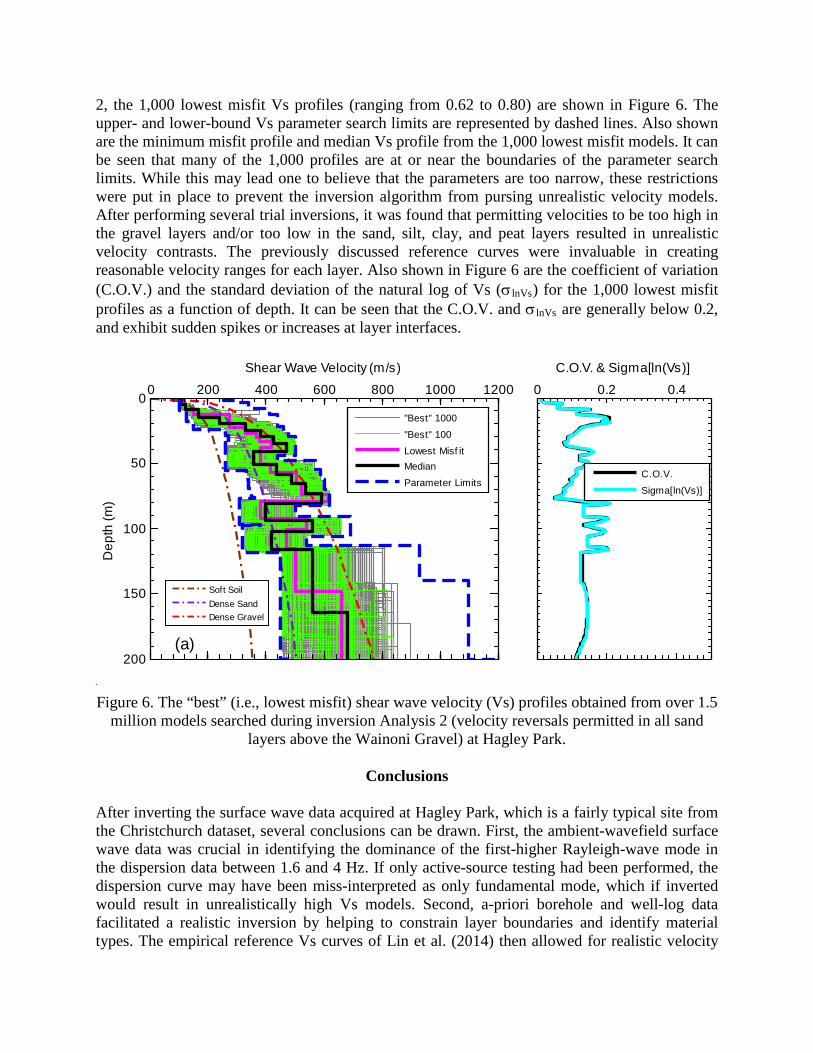
2, the 1,000 lowest misfit Vs profiles (ranging from 0.62 to 0.80) are shown in Figure 6. The upper- and lower-bound Vs parameter search limits are represented by dashed lines. Also shown are the minimum misfit profile and median Vs profile from the 1,000 lowest misfit models. It can be seen that many of the 1,000 profiles are at or near the boundaries of the parameter search limits. While this may lead one to believe that the parameters are too narrow, these restrictions were put in place to prevent the inversion algorithm from pursing unrealistic velocity models. After performing several trial inversions, it was found that permitting velocities to be too high in the gravel layers and/or too low in the sand, silt, clay, and peat layers resulted in unrealistic velocity contrasts. The previously discussed reference curves were invaluable in creating reasonable velocity ranges for each layer. Also shown in Figure 6 are the coefficient of variation (C.O.V.) and the standard deviation of the natural log of Vs (σlnVs) for the 1,000 lowest misfit profiles as a function of depth. It can be seen that the C.O.V. and σlnVs are generally below 0.2, and exhibit sudden spikes or increases at layer interfaces.

fdasf Figure 6. The “best” (i.e., lowest misfit) shear wave velocity (Vs) profiles obtained from over 1.5

million models searched during inversion Analysis 2 (velocity reversals permitted in all sand layers above the Wainoni Gravel) at Hagley Park.

Conclusions

After inverting the surface wave data acquired at Hagley Park, which is a fairly typical site from the Christchurch dataset, several conclusions can be drawn. First, the ambient-wavefield surface wave data was crucial in identifying the dominance of the first-higher Rayleigh-wave mode in the dispersion data between 1.6 and 4 Hz. If only active-source testing had been performed, the dispersion curve may have been miss-interpreted as only fundamental mode, which if inverted would result in unrealistically high Vs models. Second, a-priori borehole and well-log data facilitated a realistic inversion by helping to constrain layer boundaries and identify material types. The empirical reference Vs curves of Lin et al. (2014) then allowed for realistic velocity

Shear Wave Velocity (m/s)

Dep

th (m

)

(a)

0 200 400 600 800 1000 12000

50

100

150

200

"Best" 1000

"Best" 100

Lowest Misf itMedian

Parameter Limits

C.O.V. & Sigma[ln(Vs)]

0 0.2 0.4

C.O.V.

Sigma[ln(Vs)]

Soft SoilDense SandDense Gravel

ranges to be set for each layer in the inversion parameters. Finally, an inversion analysis which permits velocity reversals below the Riccarton, Linwood and Burwood gravel formations (Analysis 2) provides a more realistic suite of ground models than a commonly assumed normally dispersive analysis (Analysis 1). It is important to note that the minimum misfit and uncertainty estimates associated with Analysis 1 are lower than those from Analysis 2. Consequently, without utilizing geologic data, one may be inclined to believe that Analysis 1 produces better ground models. Thus, it is extremely important to understand the local geology and utilize available borehole/well-log data when inverting surface wave data in complex areas.

Acknowledgments This work was supported primarily by U.S. National Science Foundation (NSF) grants CMMI-1261775 and CMMI-1303595. However, any opinions, findings, and conclusions or recommendations expressed in this material are those of the authors and do not necessarily reflect the views of NSF. Financial support for the N.Z. Earthquake Commission (EQC) is also greatly appreciated. Mr. Robin Lee assisted with the interpretation of geologic well-log data.

References Barnes, P.M., Castellazzi, C., Gorman, A., Wilcox. S. (2011). “Submarine Faulting Beneath Pegasus Bay, Offshore Christchurch,” Prepared for the New Zealand Natural Hazards Research Platform, Contract Reference 2011-NIW-01-NHRP, 46 p.

Bettig, B., Bard, P.Y., Scherbaum, F., Riepl, J., Cotton, F., Cornou, C., and Hatzfield, D. “Analysis of dense array noise measurements using the modified spatial auto correlation method (SPAC): application to the Grenoble area.” Bollettino de Geofisica Teoria e Applicata, 42(3-4), 281-304.

Brown, L.J., Wilson, D.D., Moar, N.T., and Mildenhall, D.C. (1988). “Stratigraphy of the late Quaternary deposits of the northern Canterbury Plains, New Zealand,” NZ J. of Geology and Geophysics, 31, 305-335.

Capon, J. (1969). “High Resolution Frequency-Wavenumber Spectrum Analysis.” Proc. IEEE, 57 (8), 1408–1418.

Cox, B., Wood. C., and Teague, D. (2014). “Synthesis of the UTexas1 Surface Wave Dataset Blind-Analysis Study: Inter-Analyst Dispersion and Shear Wave Velocity Uncertainty,” ASCE Geo-Congress 2014: Geo-Characterization and Modeling for Sustainability, Atlanta, GA, 23-26 February 2014.

Dunkin J.W. (1965). Computation of modal solutions in layered, elastic media at high frequencies. Bull. Seism. Soc. Am., 55, 335–358.

Forsyth, P. J., D. J. A. Barrell, and R. Jongens (2008). Geology of the Christchurch Area. Institute of Geological and Nuclear Sciences 1:250,000 Geological Map 16, 1 sheet + 67 pp. Lower Hutt, New Zealand: GNS Science.

Haskell, N. A., 1953, The dispersion of surface waves on multilayered media: Bull. Seism. Soc. Am., 43, 17–34.

Knopoff L. (1964). A matrix method for elastic wave problems. Bull. Seism. Soc. Am., 54, 431–438.

Lee RL, Bradley BA, Ghisetti F, Pettinga JR, Hughes MW, Thomson EM. A 3D seismic velocity model for Canterbury, New Zealand for broadband ground motion simulation. Southern California Earthquake Centre (SCEC) Annual Meeting. 7-10 September 2014. Palm Springs, California, USA. (poster).

Lin, Y., Joh. S., and Stokoe, K. (2014). “Analyst J: Analysis of the UTexas 1 Surface Wave Dataset Using the SASW Methodology,” ASCE Geo-Congress 2014: Geo-Characterization and Modeling for Sustainability, Atlanta, GA, 23-26 February 2014.

Thomson, W. T. (1950). Transmission of elastic waves through a stratified solid medium: J. of Applied Physics, 21, 89–93, doi: 10.1063/1.1699629.

Wathelet, M. (2008). An improved neighborhood algorithm: parameter conditions and dynamic scaling.

Geophysical Research Letters, 35, L09301, doi:10.1029/2008GL033256.

Wathelet, M., Jongmans, D., Ohrnberger, M., Bonnefoy-Claudet, S. (2008). Array performances for ambient vibrations on a shallow structure and consequences over Vs inversion, J. Seismol, 12:1-19.

Wood. C., Ellis, T., Teague, D., and Cox, B., (2014). “Analyst I: Comprehensive Analysis of the UTexas1 Surface Wave Dataset,” ASCE Geo-Congress 2014: Geo-Characterization and Modeling for Sustainability, Atlanta, GA, 23-26 February 2014.

Zywicki, D.J. (1999). Advanced signal processing methods applied to engineering analysis of seismic surface waves. Ph.D. Dissertation, School of Civil and Environmental Engineering, Georgia Institute of Technology, Atlanta, GA, p. 357.