Embed Size (px)
Citation preview
ii
“PhDThesis” — 2012/3/26 — 19:36 — page i — #1 ii
ii
ii
Development of Mathematical
Models of a Human Virtual Ear
Thesis
Ph.D Course on:
Mechanical Engineering
Cycle XXIV(X) (2009)
Tutors:
Prof. Costantino Carmignani
Prof. Paola Forte
Eng. Francesca Di Puccio
Student:
Gaia Volandri
University of Pisa
Department of Mechanical, Nuclear and Production Engineering
SSD ING-IND/13
AcknowledgmentsI am thankful to my supervisors, Prof. Costantino Carmignani,
Prof. Paola Forte and Eng. Francesca Di Puccio whose encourage-
ment, guidance, participation and support enabled me to develop
this thesis.
I am grateful to Prof. Berrettini and Dr. Bruschini of the U.O.
Otorinolaringoiatria 2 of the S. Chiara/Cisanello hospital in Pisa,
Prof. Carlo Bartoli, Prof. Luigi Lazzeri, Eng. Armando Razionale,
Eng. Luca Nardini, Stefania Manetti and Thomas Wright. The
engineers and technicians of MAGNA Closures S.p.A., Eng. Isidoro
Mazzitelli and AM Testing s.r.l are gratefully acknowledged for their
collaboration.
I would like to show my gratitude to all of those who supported
me during the completion of the thesis.
ii
“PhDThesis” — 2012/3/26 — 19:36 — page iii — #2 ii
ii
ii
Contents
Introduction 1
1 Anatomy of the human ear 3
1.1 Outer ear . . . . . . . . . . . . . . . . . . . . . . . . 5
1.2 Middle ear . . . . . . . . . . . . . . . . . . . . . . . . 5
1.2.1 Tympanic membrane . . . . . . . . . . . . . . 6
1.2.2 Ossicular chain . . . . . . . . . . . . . . . . . 19
1.2.3 Other middle ear structures . . . . . . . . . . 23
1.3 Inner ear . . . . . . . . . . . . . . . . . . . . . . . . . 24
2 State of the Art 27
2.1 Outer and middle ear modeling approaches . . . . . . 27
2.2 Outer ear modeling . . . . . . . . . . . . . . . . . . . 30
2.2.1 Auditory canal modeling . . . . . . . . . . . . 30
2.3 Middle ear modeling . . . . . . . . . . . . . . . . . . 33
2.3.1 Tympanic membrane modeling . . . . . . . . 33
2.3.2 Ossicular chain modeling . . . . . . . . . . . . 46
2.4 Discussion on the literature survey . . . . . . . . . . 57
2.4.1 Discussion on auditory canal survey . . . . . . 57
iii
CONTENTS
2.4.2 Discussion on tympanic membrane survey . . 58
2.4.3 Discussion on ossicular chain survey . . . . . . 59
3 Auditory Canal Model 63
3.1 Methods . . . . . . . . . . . . . . . . . . . . . . . . . 64
3.1.1 Generalized finite element method (GFEM) . 66
3.1.2 Fluid structure interaction . . . . . . . . . . . 69
3.1.3 Auditory canal analysis and modeling . . . . . 71
3.1.4 Tympanic membrane analysis and modeling . 73
3.1.5 Analysis types and outputs . . . . . . . . . . 74
3.2 Results and discussion . . . . . . . . . . . . . . . . . 75
4 Tympanic Membrane Model 79
4.1 Comparison of literature finite element models . . . . 80
4.1.1 Outline of reference models . . . . . . . . . . 80
4.1.2 Analysis and modeling . . . . . . . . . . . . . 87
4.1.3 Results . . . . . . . . . . . . . . . . . . . . . . 91
4.2 Sensitivity analysis . . . . . . . . . . . . . . . . . . . 98
4.2.1 Input variables . . . . . . . . . . . . . . . . . 98
4.2.2 Results . . . . . . . . . . . . . . . . . . . . . . 99
4.3 Discussion . . . . . . . . . . . . . . . . . . . . . . . . 99
5 Ossicular Chain Model 101
5.1 Methods: a multibody model . . . . . . . . . . . . . 102
5.1.1 Basic model geometry . . . . . . . . . . . . . 106
5.1.2 Component definition . . . . . . . . . . . . . . 107
5.1.3 Model implementation . . . . . . . . . . . . . 109
5.1.4 Parameter identification procedure . . . . . . 109
5.2 Results . . . . . . . . . . . . . . . . . . . . . . . . . . 114
iv
ii
“PhDThesis” — 2012/3/26 — 19:36 — page v — #3 ii
ii
ii
CONTENTS
5.2.1 Model calibration . . . . . . . . . . . . . . . . 114
5.2.2 AML-PIL axis . . . . . . . . . . . . . . . . . . 122
5.2.3 Instantaneous axis of motion of the malleus-
incus complex . . . . . . . . . . . . . . . . . . 122
5.2.4 Relative motion at the IMJ . . . . . . . . . . 123
5.3 Discussion . . . . . . . . . . . . . . . . . . . . . . . . 125
6 Hybrid middle ear model 129
6.1 Model components . . . . . . . . . . . . . . . . . . . 130
6.1.1 Tympanic membrane finite element model . . 130
6.1.2 Ossicular chain multibody model . . . . . . . 131
6.2 Hybrid FE/MB middle ear model . . . . . . . . . . . 131
6.2.1 Parameter identification procedure . . . . . . 133
6.2.2 Sensitivity analysis . . . . . . . . . . . . . . . 133
6.3 Results . . . . . . . . . . . . . . . . . . . . . . . . . . 136
6.3.1 Tympanic membrane parameters . . . . . . . 136
6.3.2 Ossicular chain parameters . . . . . . . . . . . 137
6.4 Discussion . . . . . . . . . . . . . . . . . . . . . . . . 138
7 Psychoacoustics 143
7.1 Characteristics of sounds and hearing area . . . . . . 144
7.2 Psychoacoustic metrics and models . . . . . . . . . . 146
7.2.1 Loudness . . . . . . . . . . . . . . . . . . . . . 146
7.2.2 Sharpness . . . . . . . . . . . . . . . . . . . . 152
7.2.3 Fluctuation strength and roughness . . . . . . 154
7.2.4 Tonality . . . . . . . . . . . . . . . . . . . . . 157
7.2.5 Combined psychoacoustic metrics . . . . . . . 157
7.3 Application to power window noise evaluation . . . . 159
v
CONTENTS
7.3.1 State of the art . . . . . . . . . . . . . . . . . 159
7.3.2 Materials and experimental activity . . . . . . 161
7.3.3 Methods and models . . . . . . . . . . . . . . 162
7.3.4 Results and discussion . . . . . . . . . . . . . 164
Conclusions 167
Bibliography 195
vi
ii
“PhDThesis” — 2012/3/26 — 19:36 — page 1 — #4 ii
ii
ii
Introduction
The human ear is a complex biomechanical system, devoted to sound
reception and perception. However, some of the hearing function is
accomplished by the central nervous system.
Sound consists in a traveling wave propagating in a medium as a
mechanical wave of compression and rarefaction. Focusing on the air
medium, mammals developed a tuned system to catch (outer ear)
and transfer (middle ear) sound waves to the inner part of the ear,
where the received input is converted to electric signals and sent
to the auditory cortex. The outer ear consists of the auricle and
the auditory canal. The middle ear mainly consists in the tympanic
membrane and ossicular chain. The inner ear includes the cochlea.
The present thesis mainly focuses on the outer and middle ear.
Since the peripheral parts of the ear consists in a mechanical sys-
tem, distributed and lumped parameter models are proposed in the
literature for simulating and predicting their behavior. During the
PhD course, outer and middle ear models were developed as first
stages to build a ”virtual” ear, with the aim of understanding and
predicting the human perception of sound. The anatomy in brief
and a model-oriented review of outer and middle ear are introduced
1
CONTENTS
in §1 and §2. In details, a finite element (FE) model of the tympanic
membrane is presented in §4. A model including the auditory canal
and the tympanic membrane was developed applying standard and
generalized FE methods (§3). The multi-body (MB) approach was
adopted for the ossicular chain and supporting structures (joints,
ligaments and muscle tendons), as described in §5. The tympanic
membrane FE model and the ossicular chain MB model were com-
bined in a hybrid FE-MB model of the middle ear (§6).
The information processing in the auditory system, in terms
of preprocessing in the peripheral system (outer, middle and inner
ear) and neural processing, both including non-linearities, is a cen-
tral issue of the psychoacoustics, a branch of acoustics concerning
the quantitative correlation between the physical characteristics of
sounds and their perceptual attributes. Psychoacoustic models con-
sider the hearing function as a whole. The relationship between
physical magnitudes of the stimulus and magnitudes of the corre-
lated hearing sensations can be given either by equations or curves
of a psychoacoustic model, based on experimental evidences or jury
tests of perception.
As an application of the psychoacoustic approach, an experimen-
tal and theoretical activity on power window noise was conducted
(§7) during the last year of the PhD course within a project in col-
laboration with MAGNA Closures S.p.A.
2
ii
“PhDThesis” — 2012/3/26 — 19:36 — page 3 — #5 ii
ii
ii
Chapter 1
Anatomy of the human ear
Sound consists in a traveling wave (transmitted through a solid,
liquid, or gas) which could be easily described by means of the time-
varying sound pressure [1].
The human auditory system responds in the 20 Hz−20 kHz fre-
quency range (conventionally assumed audible frequencies [2]) and
in the 10−5 (threshold in quiet)−102 Pa (threshold of pain) values
of sound pressure, identifying also pitch, timbre, and direction of a
sound [1].
Focusing on the air medium (343 m/s speed of sound at 20C and
1 atm), mammals developed a tuned system to catch (pinna/auricle)
and transfer sound waves to the proper auditory organ (cochlea),
where the received input is sent to the auditory cortex, passing
through the acoustic ways.
Three parts are conventionally identified in the terrestrial mam-
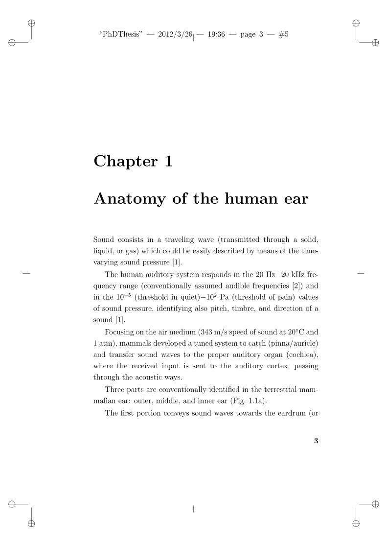
malian ear: outer, middle, and inner ear (Fig. 1.1a).
The first portion conveys sound waves towards the eardrum (or
3
Anatomy of the human ear
Figure 1.1: A schematic representation of human a) outer and middle
ear, b) middle and inner ear (Gray’s anatomy table [3]).
tympanic membrane, TM), amplifying sound pressure in the fre-
quency range 20 Hz - 20 kHz. The middle ear transfers the vibra-
tions from the TM to the cochlea in the inner ear, a spiral-shaped
organ responsible for the transduction of acoustic signals into neuro-
logical signals [4, 5]. Each part of the auditory apparatus has a very
peculiar behavior, involving mainly fluid-structure interaction, me-
chanical vibrations, neurosignal generation and transmission. Some
features of this complex biomechanical system have still to be com-
pletely understood and are investigated by experimental and numer-
ical simulation. However both approaches share difficulties mainly
due to the reduced size of the elements and the differences between
animal and human apparatus that make extrapolation of results un-
feasible.
The present thesis mainly focuses on the outer and middle ear.
4
ii
“PhDThesis” — 2012/3/26 — 19:36 — page 5 — #6 ii
ii
ii
1.1 Outer ear
The investigation of inner ear currently constitutes a future devel-
opment of our study.
1.1 Outer ear
The outer ear consists of the auricle and the auditory canal (AC).
The auricle picks up airborne vibratory waves. The AC channels
them to the middle ear. It is closed at the medial end by the TM,
which can be considered either part of the outer or the middle ear.
Its ”S-shaped” morphology, facilitates the sound wave channeling
and amplifies some resonance frequencies.
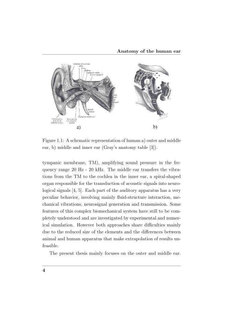
1.2 Middle ear
The middle ear is an 1-2 cm3 air-filled space in the temporal bone,
which is normally sealed laterally by the TM or eardrum, including
three small bones (the ossicles: malleus, incus and stapes), which
constitute the ossicular chain (OC) and related structures, ligaments,
muscles, joints and nerves, involved in sound conduction[3, 6], Fig.
1.2.
The OC builds a mechanical lever-action connection between the
air-actuated TM and the fluid-filled cochlea. As the direct contact
between air and cochlear fluids of the inner ear would not succeed in
stimulating the perilymph of the inner ear to any significant extent,
the middle ear primary function is to act as an impedance matching
system between the low/high impedance media, air and cochlear
fluids respectively. This function is achieved in two ways: the lever
5
Anatomy of the human ear
Figure 1.2: Middle ear schemes. (Reprinted with permission from
http://hearingaidscentral.com/howtheearworks.asp)
action of the OC, reducing the displacement at the oval window
(OW), with respect to the one at the apex of the TM (umbo, of
about 1:1.3 - 1:3.1, and the ratio of the areas of the TM and the
stapes footplate (SFP) which is about 27 [4].
1.2.1 Tympanic membrane
In the literature detailed descriptions of the human and animal TM
from different laboratories and investigators are available; the great
variations of the TM among different species elucidate the structure-
function relationship of the morphological and physical features of
the TM, which are differently tuned for the sound transmission in
6
ii
“PhDThesis” — 2012/3/26 — 19:36 — page 7 — #7 ii
ii
ii
1.2 Middle ear
varying frequency ranges and environments for different species, e.g.
[7, 8, 9].
The TM is placed in the ear canal with a particular orientation,
which allows it to have a larger surface than the ear canal section
itself. A typical angle between the human TM and the superior and
posterior wall of the ear canal is 140 deg, while between the TM and
the inferior and anterior wall is 30 deg [10].
The periphery of the TM is firmly anchored to the wall of the
tympanic cavity, around most of its circumference, by a fibro -
cartilaginous ring called the annular ligament (AL) or tympanic an-
nulus (TA)[11] (Fig. 1.3a-b). This ligament is a fibrous thickening
firmly attached to a sulcus in the bony tympanic ring, except superi-
orly where it separates the two main regions (or submembranes [12])
of the TM called the “pars tensa” (PT) and the “pars flaccida” (PF).
The PT is a multi-laminar membrane which covers almost the whole
extension of the TM with an outline varying from approximately cir-
cular to a more or less elongated ellipse across species. The PF lies
in the superior region and its size is variable in mammals; the human
PF is moderately small and it differs in anatomy and function from
the PT since it is thicker and much more compliant than the rest
of the membrane [9]. In the superior part of the tympanic ring, a
deficiency in the temporal bone sulcus, called the notch of Rivinus,
forms an attachment for the PF.
The TM is attached to the manubrium of the malleus, which
stretches from a point on the superior edge of the TM to its center,
the umbo (Fig. 1.3a-b). The umbo is considered a fundamental
reference point, frequently mentioned in model result presentation.
The manubrium of the malleus may be placed symmetrically, or
7
Anatomy of the human ear
closer to the antero-superior edge of the TM. The attachment of the
manubrium to the TM varies along its length: the lateral process of
the malleus and the umbo are firmly attached, while in the midway
region, between the lateral process and the umbo, the manubrium
separates slightly from the TM [10].
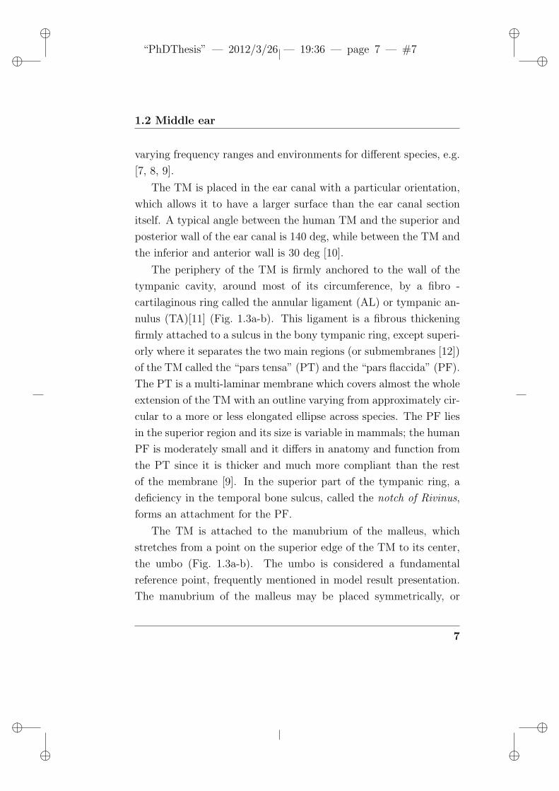
The TM (Fig. 1.3a-b) is almost oval in shape and conical in cross
section, with the apex pointing medially towards the middle ear.
Its vertical axis ranges from 8.5 to 10 mm while the horizontal axis
ranges from 8 to 9 mm with a mean total area of 85 mm2 [10]. In
physiological conditions, its curved conical shape has a cone angle of
132−137 deg [13] with a cone depth included in the range 1.42 − 2
mm [14, 15].
Figure 1.3: a) A schematic representation (Gray’s anatomy table [3]),
b) a medial view of the TM (reprinted from [13] with permission from
Elsevier). c) Contour plot of the thickness distribution of an entire
human TM (reprinted from [16] with permission from Elsevier).
A critical feature for vibratory behavior is the TM thickness as
it describes the mass distribution in the rapidly vibrating TM and
also influences the effective TM stiffness. An example of thickness
8
ii
“PhDThesis” — 2012/3/26 — 19:36 — page 9 — #8 ii
ii
ii
1.2 Middle ear
distribution map is shown in Fig. 1.3c. At present, accurate and de-
tailed data available concerning the thickness of the human TM are
still few [17]. The first measurements are due to [18], who observed a
non-uniform thickness ranging from 30 to 120 µm. Lately, until the
90’s other thickness measurements on human TM were performed
[19, 20, 21, 22, 23, 24], typically based on conventional light or elec-
tron microscopy on a few points of histological sections of non-fresh
material. However, these data show large differences, probably due
to pre-treatment effects in the sample preparation. Only recently a
new method to draw a thickness distribution map of an untreated
TM, based on confocal laser microscopy, was introduced for the cat
in [17]. This method was applied in [25] to three fresh human sam-
ples obtaining a great inter-individual variability in mean thickness
values (40, 50 and 120 µm), thus stressing that there is no typical hu-
man TM thickness. However the authors identified similar features
in terms of relative thickness variations in all samples: a large thin
portion in the infero-posterior quadrant, with a gradual thickening
towards the superior portion, and an anterior part thicker than the
posterior one.
In the through-thickness section of the TM, a multi-layer fiber
structure consisting of distinct layers, varying in density, thickness,
composition and arrangement in different regions, can be identified.
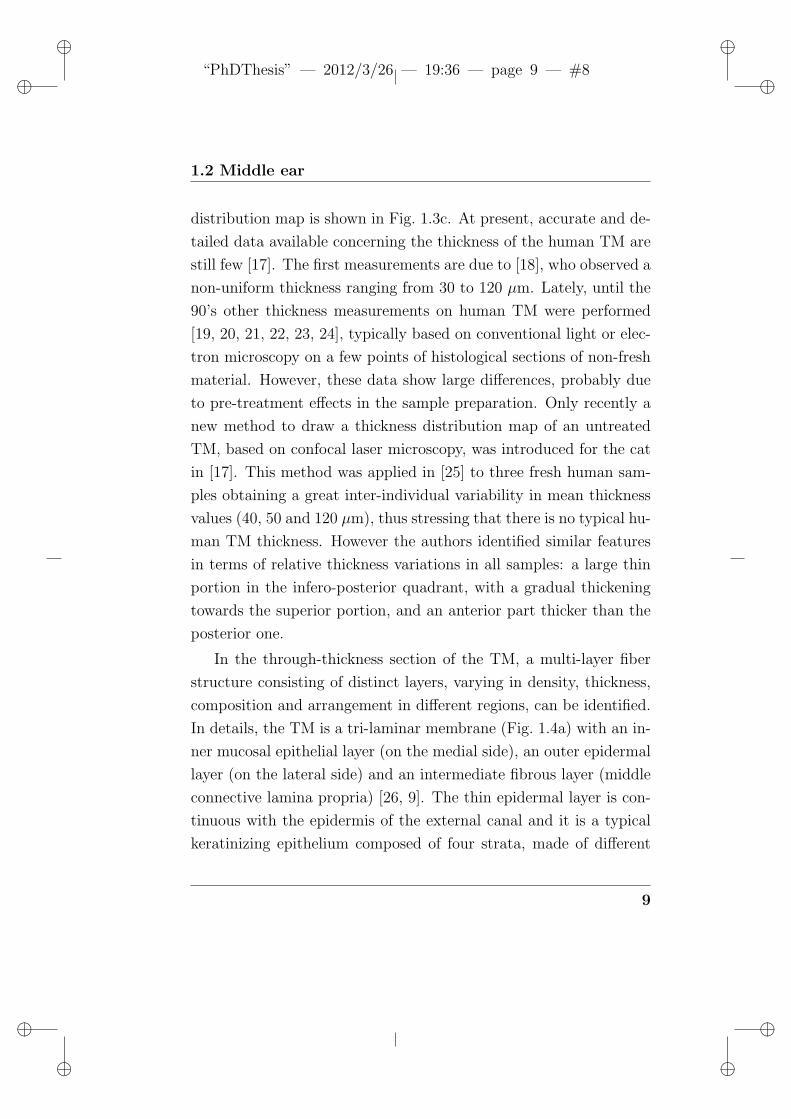
In details, the TM is a tri-laminar membrane (Fig. 1.4a) with an in-
ner mucosal epithelial layer (on the medial side), an outer epidermal
layer (on the lateral side) and an intermediate fibrous layer (middle
connective lamina propria) [26, 9]. The thin epidermal layer is con-
tinuous with the epidermis of the external canal and it is a typical
keratinizing epithelium composed of four strata, made of different
9
Anatomy of the human ear
Figure 1.4: a) A schematic diagram of a typical TM cross-section
through PT showing the arrangement and thickness of different lay-
ers (reprinted from [13] with permission from Elsevier). b) Schematic
of the fiber orientation of human TM.
cell types [7]. The mucosal layer is a very thin layer of cells. The
differences in the PT and PF lie in the structure of their lamina
propria [10], whose cell and biological molecular aspects, vascular
and nerve supply are deeply described in [7]. The lamina propria
of the PT consists of two subepidermal connective tissue layers, be-
tween which there are two collagenous layers with radial and circular
fiber orientation (Fig. 1.4b). The radial fibers become more packed
as they converge on the manubrium, while the circular fiber layer
grows thicker towards the periphery. These collagen fibers exhibit a
viscoelastic and orthotropic behavior with membrane (or in-plane)
properties different from through-thickness (or out-of-plane) proper-
ties [13]. Parabolic and transversal fibers have been identified in the
PT, too. The parabolic fibers arise from near the lateral process of
the malleus and extend downwards in a parabolic course to the an-
10
ii
“PhDThesis” — 2012/3/26 — 19:36 — page 11 — #9 ii
ii
ii
1.2 Middle ear
terior or posterior quadrant. The transversal fibers are short fibers
running horizontally in the inferior quadrant. The lamina propria of
the PF is made up with loose connective tissue containing collagen
and elastic fibers [10].
In Fig. 1.4a ranges of thicknesses values for the entire membrane
as well as for the layers in the PT portion are shown. It is worth not-
ing that the overall membrane thickness is non-uniform but tapered
from the periphery to the umbo; fiber layers follow the same trend
but, whereas the circumferential fiber layer is tapered to nearly-
zero thickness at the umbo, the radial fiber layer thickness decreases
slightly.
As described in [8], the fibers of the human TM extend in a
continuous manner towards the periphery forming the AL.
Experimental activity from the literature
Many experimental data on the mechanical characterization and vi-
bration response of the TM can be found in the literature since the
40’s, e.g. [27, 28, 19]. The availability of these data is crucial for
model parameter identification and result validation. However it is
worth noting that the complex structure and the small dimensions of
the TM (around 10 mm in diameter and 0.08 mm in thickness) hin-
der the assessment of its mechanical and material properties as well
as its constraints, morphological characteristics, static displacement
under load and sound-induced motion. Despite the fact that mam-
malian TM’s differ in some morphologic and material properties,
animal TM have been widely investigated with the aim of general-
izing the analysis results to the human case. In particular the most
11
Anatomy of the human ear
common animals in hearing research are gerbils and cats, although
also rabbits, guinea pigs and mouses are commonly investigated [9].
In this paragraph a brief outline of published experimental results
is reported. Further details on experimental data can be found in
[8, 9].
Material characterization
Material characterization of the TM tissues still represents a de-
bated issue, due to the variety of tests, typically in vitro, but also in
vivo. Mechanical properties of the human TM were first measured
by [27, 28] since the 40’s and by [19]. They obtained very different
Young’s moduli (20 vs. 40 MPa) because values are strongly de-
pendent on the precision of thickness measurements which are very
critical. [29] conducted uniaxial tension tests of human TM samples
obtaining a nonlinear stress-strain curve with a tangent modulus
similar to v. Bekesy at about ±8% of strain. Their results were
re-interpreted by [30]. Other uniaxial tensile, stress relaxation, and
failure tests on fresh human cadaver TM specimens were published
only recently by [26] obtaining a Young’s modulus varying from 0.4
to 22 MPa over the stress range from 0 to 1 MPa, in good agree-
ment with [29]. All previously mentioned works employed rectan-
gular strip samples from human TM deducing elasticity parameters
under the hypotheses of isotropy, homogeneity and uniform thick-
ness, although extracted taking into account the circumferential and
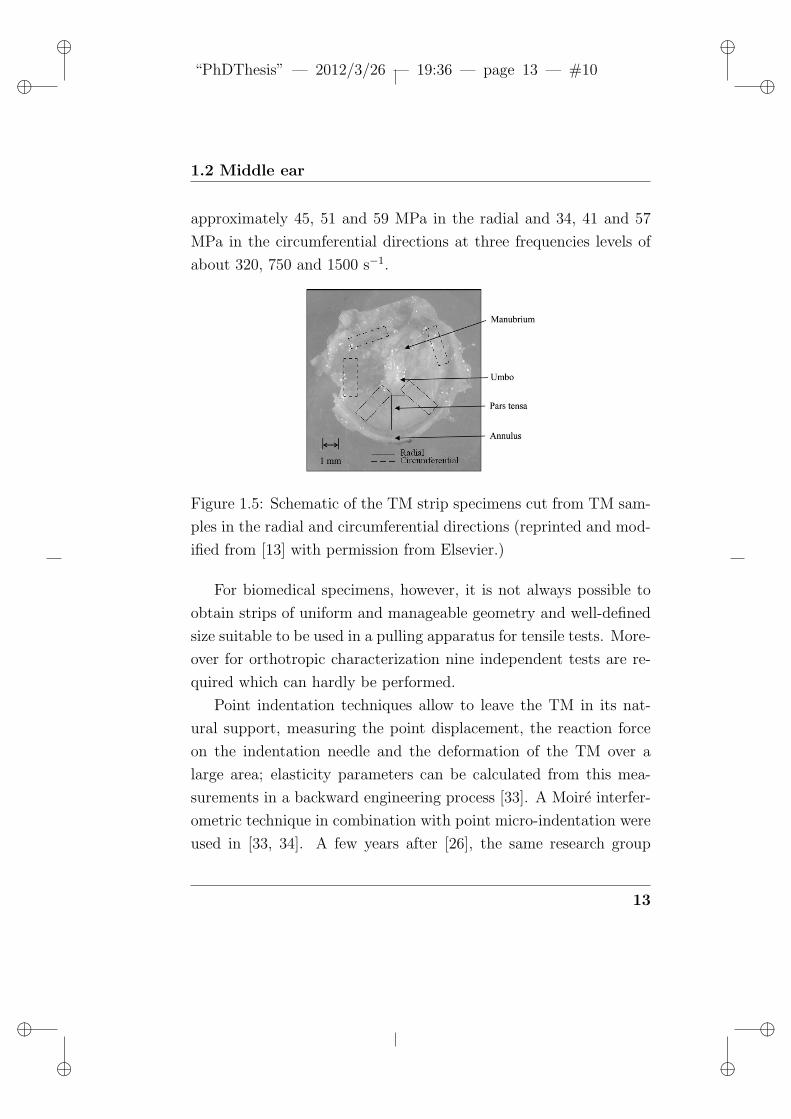
radial directions. An example of a typical strip sample is indicated
in Fig. 1.5 on an image from [13].
To the best of the authors’ knowledge, the only works performing
orthotropic characterization by means of tensile tests are [31, 32]
that propose high strain rates tests obtaining Young’s moduli of
12
ii
“PhDThesis” — 2012/3/26 — 19:36 — page 13 — #10 ii
ii
ii
1.2 Middle ear
approximately 45, 51 and 59 MPa in the radial and 34, 41 and 57
MPa in the circumferential directions at three frequencies levels of
about 320, 750 and 1500 s−1.
Figure 1.5: Schematic of the TM strip specimens cut from TM sam-
ples in the radial and circumferential directions (reprinted and mod-
ified from [13] with permission from Elsevier.)
For biomedical specimens, however, it is not always possible to
obtain strips of uniform and manageable geometry and well-defined
size suitable to be used in a pulling apparatus for tensile tests. More-
over for orthotropic characterization nine independent tests are re-
quired which can hardly be performed.
Point indentation techniques allow to leave the TM in its nat-
ural support, measuring the point displacement, the reaction force
on the indentation needle and the deformation of the TM over a
large area; elasticity parameters can be calculated from this mea-
surements in a backward engineering process [33]. A Moire interfer-
ometric technique in combination with point micro-indentation were
used in [33, 34]. A few years after [26], the same research group
13
Anatomy of the human ear
[35, 13] characterized the viscoelastic behavior of the TM by nano-
indentations, measuring in-plane (clamping the sample on a circular
hole) and through-thickness (placing the sample on a relatively rigid
solid substrate) Young’s relaxation moduli; [35] obtained steady-
state values for the in-plane moduli of 17.4 MPa and 19 MPa for
posterior and anterior TM samples, respectively (comparable with
those obtained by [28]) and a value of through-thickness modulus of 6
MPa. In [13] nanoindentation was applied to sections cut from fresh-
frozen human cadaveric TMs obtaining Young’s relaxation modulus
values ranging in approximately 25.7-37.8 MPa, close to values ob-
tained by [19] and [28]. On the contrary, in [36] the nanoindentation
technique is applied to the intact TM (i.e. without sectioning) and,
using a 12 µm thickness, an effective ∼ 21 MPa average Young’s
modulus of the PT was found, with the assumptions of isotropy and
homogeneity.
In [13, 37, 36, 34, 12] an inverse problem solving methodology was
employed using the FE method to determine material parameters;
in this approach material models are assumed in advance (e.g. linear
elastic isotropic/orthotropic or hyperelastic material) and material
parameters determined by inverse/optimisation procedures. In par-
ticular, the recent work of [12] presents an elastic characterization of
the gerbil PF via inverse analysis of in situ static pressure inflation
experiments assuming the Veronda-Westmann hyperelastic model.
The elasticity of human TM has been experimentally investigated
in vitro by many authors. However, methods for in vivo clinical ex-
periments investigating these elastic properties are relatively few and
not readily comparable. Different measurements of elasticity have
been reported by [38] who investigated the pressure-volume relation-
14
ii
“PhDThesis” — 2012/3/26 — 19:36 — page 15 — #11 ii
ii
ii
1.2 Middle ear
ship of the middle ear system applying pressure changes in the ear
canal; however, no single measure of elasticity was extracted from
their experiments. Based on [38], a more recent pressure-volume
method has been developed and improved by [39]. As a noteworthy
example of a recent in vivo material characterization, [40] should
be mentioned; in this study the areal modulus (i.e. the relationship
between membrane tension and change of the surface area relative
to the undeformed surface area, measured by means of an hydraulic
system including pumps and tubes) is estimated in a group of 20
normal subjects, based on response of the human TM to quasi-static
pressure changes; the Young’s modulus values, calculated dividing
the areal moduli (derived from linear conditions) by the membrane
thickness, result a factor 2-3 smaller than previously found in vitro
by [27, 29].
For completeness, it is worth noting that the presence of prestrain
might have an influence on the mechanical behavior of the TM as
described by [28, 19].
Vibration response and displacement measurements
Several experimental investigations focus on measuring of TM
static displacement and sound-induced vibrations with various (mostly
interferometric) techniques. Tympanometry is a clinical in vivo mea-
sure of the average motion of the entire TM and does not distinguish
the motion of different locations, although useful for aiding in the
differential diagnosis of hearing diseases.
By contrast, interferometric techniques and, in particular, a com-
mercially available laser Doppler vibrometer (LDV) (or interferom-
eter, or velocimeter) is a non-contacting device capable of measur-
ing the displacement amplitude of TM vibrations down to 1 nm.
15
Anatomy of the human ear
Sound-induced motion of the umbo has often been studied through
measurements of umbo displacement by LDV in the “piston-like”
direction. LDV techniques are employed in recent literature in vivo
[41, 42, 43, 44, 45] and in vitro [46, 47, 48, 49, 50]. The umbo velocity
transfer function (magnitude and phase angle) is the most common
output [41, 42, 43, 46, 47]; [41] estimated, by means of LDV measure-
ments in 80 normal hearing ears of 56 subjects, a magnitude ranging
over a little more than a factor of 10 (±10 dB) and a range of angles
varying from about 45 deg at 250 Hz to more than 400 deg at the
highest frequencies. The authors also describe a complex behavior
similar to previously published measurements of umbo velocity in
live ears: at frequencies below 0.7 kHz, the umbo velocity transfer
function has a magnitude proportional to frequency and an angle
between 45 and 90 deg; in the 1-2 kHz range, the transfer functions
have a nearly constant magnitude and an angle near 0 deg; above 3
kHz, the increase in magnitude and the increasing phase lag between
velocity and pressure suggest a complex relationship between the ear
canal sound pressure and the velocity measured near the umbo. In
[43] the LDV determined umbo-velocity transfer functions of ears
with sensorineural hearing loss are compared with the same mea-
surements on 56 ears from 56 normal-hearing subjects taken from
[41]; their results show a wide range of variability with a magni-
tude range at any one frequency of a little larger than an order of
magnitude (20 dB), and an angle range that increases with stimulus
frequency, from ±10 deg at 0.3 kHz to ±180 deg at 6 kHz.
Although the umbo motion is a crucial input to the ossicular
sound-conduction system, it is worth noting that vibrations of the
entire TM surface contribute to vibration of the manubrium and
16
ii
“PhDThesis” — 2012/3/26 — 19:36 — page 17 — #12 ii
ii
ii
1.2 Middle ear
ossicular sound conduction. For these reasons most detailed descrip-
tions of the motion of the mammalian TM were obtained by means
of time-averaged holograms [51, 52, 53, 54]. Time-averaged holog-
raphy and holographic interferometry enable to record the complete
vibration pattern of a surface within several seconds [55, 51, 52, 56].
Only few authors report the mode shapes (e.g. [16, 10]); [10], on
the basis of a scanning LDV (SLDV), concludes that at low frequen-
cies the TM assumes simple mode shapes without nodes, showing a
piston-like movement of the umbo, while at higher frequencies the
deformation pattern becomes more and more complex showing lots
of peaks and valleys above 4 kHz; due to this highly fragmented
movement pattern the movement of the umbo results drastically re-
duced.
Over the last years several research groups [57, 58] have worked
to apply modern computer-assisted high-speed opto-electronic holog-
raphy (OEH) to the study of the vibration of the TM, very suit-
able for in vivo investigations. In [58] OEH is employed to produce
time-averaged holograms that describe the magnitude of the sound-
induced motion of the surface of the TM. After using time-averaged
holography, that is insensitive to the phase of motion relative to the
sound stimulus phase, the same authors in [59] describe results using
stroboscopic holography [57, 60, 61] to study sound-induced motion
of the TM. With stroboscopic holography both the amplitude and
phase of the dynamic deformations of the TM over the full field of
view can be quantified.
Although the frequency response function varies across the TM
surface, a reference point is commonly selected (usually the umbo or
a point lying midway between the tip of the malleus and the annulus)
17
Anatomy of the human ear
[62]. In [63] the TM displacement distribution, the maximum value,
and the displacement value at the umbo are reported: ranging from
0.2 to 0.4 µm and equal to about 0.050 µm at approximately 120
dB and 80 dB, respectively. Most authors [15, 62, 64, 10, 65, 66, 67]
report experimental and model-derived frequency response curves
(umbo displacement or velocity vs. frequency, sometimes normalized
by the input sound pressure value) as a crucial output of analysis.
Concerning undamped modal frequencies, several authors observe
a first resonance frequency in the umbo displacement frequency re-
sponse typically ranging from 0.9 kHz to 1.4 kHz [10, 15, 16] or at
about 1.5 kHz [62] in experimental (but also in numerical) inves-
tigations. In [16] a peak around 1 kHz is clearly identified in the
numerical curves while it is less evident in the experimental ones.
[10] concludes that the results of many experimental modal analyses
performed on the TM (with different intact/removed structures of
the middle and inner ear) show great variability from specimen to
specimen, particularly in the position of the main poles (e.g. the
first resonance frequency ranges from about 344 to 1385 Hz).
Many authors agree on considering the TM frequency response
below 1 kHz reasonably flat [62], exhibiting a resonance at about
1-1.5 kHz; above this peak the response decreases with frequency,
showing other resonances at higher frequencies [10]. Some authors
identify a significant resonance at about 3-4 kHz, due to the presence
of the ear canal, which is evident in some experimental data and not
in others, since this resonance peak will depend on the length and
shape of the ear canal and also on the location of the sound delivery
system [11, 65].
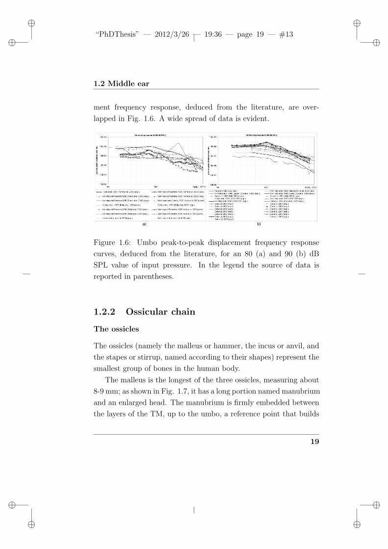
Several experimental curves of the umbo peak-to-peak displace-
18
ii
“PhDThesis” — 2012/3/26 — 19:36 — page 19 — #13 ii
ii
ii
1.2 Middle ear
ment frequency response, deduced from the literature, are over-
lapped in Fig. 1.6. A wide spread of data is evident.
Figure 1.6: Umbo peak-to-peak displacement frequency response
curves, deduced from the literature, for an 80 (a) and 90 (b) dB
SPL value of input pressure. In the legend the source of data is
reported in parentheses.
1.2.2 Ossicular chain
The ossicles
The ossicles (namely the malleus or hammer, the incus or anvil, and
the stapes or stirrup, named according to their shapes) represent the
smallest group of bones in the human body.
The malleus is the longest of the three ossicles, measuring about
8-9 mm; as shown in Fig. 1.7, it has a long portion named manubrium
and an enlarged head. The manubrium is firmly embedded between
the layers of the TM, up to the umbo, a reference point that builds
19
Anatomy of the human ear
the tightest connection between the OC and the TM. The head of
the malleus is connected to the body of the incus through the incudo-
malleolar joint (IMJ), which plays a key role in the dynamic behavior
of the OC.
The incus projects posteriorly by a short process and inferiorly by
a long process which terminates in the lenticular process, the lateral
aspect of the incudo-stapedial joint (ISJ) while the medial aspect is
provided by the head of the stapes.
The neck of the stapes splits medially into two crura attached to
the SFP, which has the form of a slightly irregular oval. The SFP
is circumferentially connected to the cochlear wall by fibrous con-
nective tissue known as the annular ligament or stapedio-vestibular
joint (SVJ) that constitutes a peripheral suspension of the whole
OC. The SFP occupies the oval window (OW), an opening between
the tympanic cavity and the inner ear. Closed by a membrane, the
round window is situated below and behind the OW and vibrates
with opposite phase, allowing the movement of the cochlear fluids
[3].
Joints
The OC is connected to the TM on the lateral side and to the OW
on the medial side and is bound together by two synovial joints, the
IMJ and the ISJ, Fig. 1.7.
The IMJ may be classified as a saddle-type joint with curved
reciprocal concave-convex surfaces. As nicely reported by Willi in
its comprehensive reviews on the IMJ functionality [68, 69], in its
comprehensive review on the IMJ functionality, the function of this
20
ii
“PhDThesis” — 2012/3/26 — 19:36 — page 21 — #14 ii
ii
ii
1.2 Middle ear
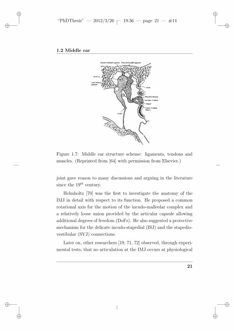
Figure 1.7: Middle ear structure scheme: ligaments, tendons and
muscles. (Reprinted from [64] with permission from Elsevier.)
joint gave reason to many discussions and arguing in the literature
since the 19th century.
Helmholtz [70] was the first to investigate the anatomy of the
IMJ in detail with respect to its function. He proposed a common
rotational axis for the motion of the incudo-malleolar complex and
a relatively loose union provided by the articular capsule allowing
additional degrees of freedom (DoFs). He also suggested a protective
mechanism for the delicate incudo-stapedial (ISJ) and the stapedio-
vestibular (SVJ) connections.
Later on, other researchers [19, 71, 72] observed, through experi-
mental tests, that no articulation at the IMJ occurs at physiological
21
Anatomy of the human ear
sound pressure levels (belonging to the 0 120 dB, more typically 80
90 dB, Sound Pressure Level (SPL) range) and at low frequency (<
0.3 kHz), leading to the conclusion that the malleus and the incus
vibrate as a single rigid body [11]. Only at extremely high sound
pressure levels or high frequencies, above 0.3 kHz and particularly
above 10 kHz [72], was any articulation observed, probably to pro-
tect the inner ear [73]. In this sense, in [74] Huttenbrink illustrated
the gliding motion between the malleus and the incus when exposed
to changes in static air pressure, which can cause displacements of
up to 1 mm in the OC, as opposed to the physiologic microscopic
acoustic vibrations.
Other indications against the fixed IMJ assumption were pre-
sented in the last decade by two research groups [69, 68, 75, 10].
Experimental evidences reported in [69, 68, 10] elucidate a relative
motion at the IMJ with three main contributions: the translation in
the ”piston-like” direction (from the umbo to the stapes, orthogonal
to the plane of the OW membrane) and the two rotations around
the other orthogonal axes. A mobility of the IMJ in the 75-90 dB
SPL range, affecting the middle ear transfer function, was assessed
in [69]. Moreover, Ferrazzini [10] showed a slippage of about 20 nm
between the malleus and incus even at low or moderate frequencies
(75-90 dB SPL).
The malleus and the incus have been long believed to rotate as
a single rigid body about a fixed axis at least at low frequencies
[28, 76] while a highly frequency dependent rotation axis has been
identified above 1 kHz [71, 11, 77].
The ISJ is a synovial shallow ball-and-socket type or enarthrodial
joint [6, 74]. There is a general agreement on the anatomy of this
22
ii
“PhDThesis” — 2012/3/26 — 19:36 — page 23 — #15 ii
ii
ii
1.2 Middle ear
joint, which represents the weakest point of the chain and, therefore,
is the most subjected to dislocations and fractures [78].
1.2.3 Other middle ear structures
The human middle ear includes also various ligaments, muscles, ten-
dons, nerves and folds of mucous membrane (Fig. 1.7) which sur-
round and support the ossicles restraining their vibratory movements
[6, 3, 19].
The malleus is held in place by the TM and also by four liga-
ments: the superior ligament (SML), the anterior ligament (AML),
the posterior ligament (PML) and the lateral ligament (LML), named
after their relative position with respect to the malleus itself. The
SML suspends the malleus from the superior wall of the tympanic
cavity. The AML connects the neck of the malleus to the anterior
wall of the tympanic cavity, while the LML connects the lateral side
of the TM. The incus is suspended and connected to the cavity wall
by its superior ligament and its posterior ligament (PIL), respec-
tively. The base of the stapes (SFP) is connected around its rim to
the OW by the stapedial annular ligament (SAL).
Besides, the middle ear contains two muscles, the tensor tympani
(TT) (whose tendon is attached to the manubrium of the malleus)
and the stapedius muscle (whose tendon (ST) is attached to the neck
of the stapes). As reviewed in [6], these muscles were long believed
to have a protective role, contracting when the middle ear is ex-
posed to high sound intensities. This ”protection theory” has been
widely criticized because of an observed noticeable time gap between
acoustic stimulation and contraction of the muscles [19]. Alterna-
23
Anatomy of the human ear
tive theories have been proposed for the reflexive middle ear muscle
contraction (acoustic reflex), as the ”fixation theory”, suggesting
that muscles maintain the appropriate positioning and rigidity of
the OC, and the ”accommodation theory”, stating that the muscle
action maximizes the absorption of sound energy. Another theory
proposes that the reflex function consists in improving the dynamic
range by attenuating low-frequency sounds. Huttenbrink [79] stated
that the ”fixation theory” is not verified and suggested a protective
role in terms of maintenance of the circulation of the synovial fluid
in the OC joints.
The TT and the ST muscles are innervated by the trigeminal
and facial nerves, respectively. The chorda tympani nerve branches
from the facial nerve and crosses the tympanic cavity between the
malleus and the incus without actually attaching to the ossicles [80].
The mechanical properties of these soft tissue structures have
been investigated and debated in the last years [81, 82, 83], due to
the fact that soft tissues usually show viscoelastic behavior in their
physiological operating range.
1.3 Inner ear
The inner ear consists of the bony labyrinth, a system of passages
mainly comprising two functional parts: the cochlea (a spiral-shaped
organ responsible for the transduction of acoustic signals into neu-
rological signals) and the vestibular system, devoted to balance.
The inner ear is mentioned for completeness as it constitutes a
fundamental stage in the hearing function. It will not be referenced
24

ii
“PhDThesis” — 2012/3/26 — 19:36 — page 25 — #16 ii
ii
ii
1.3 Inner ear
in the following since the present thesis focuses on outer and middle
ear.
25

Anatomy of the human ear
26
ii
“PhDThesis” — 2012/3/26 — 19:36 — page 27 — #17 ii
ii
ii
Chapter 2
State of the Art
The following literature survey concerns the outer and middle ear.
An extensive model-oriented review was conducted focusing on the
AC, the TM and the OC.
2.1 Outer and middle ear modeling ap-
proaches
Several modeling (in particular bioengineering) approaches have been
applied over the past fifty years or so, for simulating and predicting
the dynamic behavior of the human hearing organ or prosthetic de-
vices in physiological or pathological/post-surgical/post-traumatic
conditions, as reviewed by [14].
The published models can be mainly classified into two broad
categories [84]:
• lumped parameter models, including electro-acoustical ana-
27
State of the Art
logue circuit models [78, 84], electronic and signal processing
based models [85], mechanical [86, 87] or MB [88, 89] models;
• distributed parameter models, mainly represented by the FE
method, widely applied since 1978 [90], and, extensively, in re-
cent years [15, 91, 92, 93, 94, 95, 96, 97, 67, 98, 99, 100, 65,
64, 66, 62, 101, 16, 102, 103, 104]due to their capability of in-
corporating the complex geometries and the non-homogenous,
anisotropic material (important when the TM is included in
the model).
Three numerical solution techniques for nonlinear eardrum-type
oscillations (the target function technique, the multiple-parameter
technique and the direct integration technique) are proposed in [105].
A numerical simulation of the dynamical properties of the TM is
presented also in [106] employing a superposition of waveforms as a
model for describing the the vibratory patterns of the coupled system
of the tympanum-malleus. A time-domain wave model of the TM
was proposed in [84].
The first FE models of the TM were proposed by Funnell et al.
since the 70’s [90, 107, 108, 109, 110, 91, 111, 112, 113, 114, 34, 37]. A
complete computer-aided design (CAD) and FE model of the human
middle ear was published also as a patent application in 2006 by Gan
et al. [96, 97, 15, 115, 95, 116, 94, 117], extended in 2007 by adding
an uncoiled cochlear model. A FE model of the human middle ear
was developed in 2006 by Lee et al. [98, 99, 100, 118, 119], who
recently [67] have added a “third chamber” (the mastoid cavity) to
the “two-chamber” model proposed by Gan et al. [95]. A complete
FE model of the human middle ear was proposed by Prendergast
28
ii
“PhDThesis” — 2012/3/26 — 19:36 — page 29 — #18 ii
ii
ii
2.1 Outer and middle ear modeling approaches
et al. [120, 121, 64, 11, 65, 122] in 2000 and used firstly to analyse
the normal middle ear and, secondly, to analyse both PORP and
TORP prostheses; an application aimed at ventilation tube design
is reported in 2008 [122]. In the same years the group of Koike et al.
developed and applied an FE model to evaluate geometric variability
and different mobility of the human middle ear [101, 16, 10, 102, 14].
Other interesting FE modeling approaches, appeared between 2001
and 2010, focusing on the human TM are reported in [62, 123, 66,
63, 103].
A crucial problem in modeling is the trade-off between the com-
putational burden and the level of detail or approximation. On the
one hand, a FE approach can give insight into the mechanical be-
havior of the single ear component, although leading rather complex
models, as observed in [73]. Moreover, as material input data are
often scattered or unavailable, due to the difficulties of experimental
investigations a model calibration is required, which can be a chal-
lenging task. On the other hand, the simplicity of analogue models
with few degrees of freedom, based only on impedance measure-
ments, make them convenient to simulate specific aspects of acous-
tic signal transmission but they provide limited information with
respect to the complexity of the actual biological structure.
A mechanical lumped-parameter rigid-body model could repre-
sent an intermediate alternative that simplifies the joint modeling
and provides good accuracy at a low computational cost since only
the essential dynamic aspects are considered. As a drawback, un-
doubted difficulties arise in the estimation of patient-specific geo-
metric parameters. The MB approach is justified, if applied to the
ossicular chain of the middle ear, as for every measured ossicle the
29
State of the Art
first natural frequency is far away from the audible frequency range,
filtered by the TM, so that the ossicles can be considered as rigid
bodies [73, 10, 124]. As recently commented in [125], such assump-
tion is no longer correct for some thin parts of the ossicles under
particular conditions, e.g. quasi-static large sound pressures due to
altitude or meteorological changes, especially in animals.
2.2 Outer ear modeling
2.2.1 Auditory canal modeling
Several papers were collected concerning the AC modeling [15, 95,
116, 94, 65, 122, 66, 67, 14, 111, 126, 127, 128, 129, 130, 131, 132].
Geometry
Several solutions have been reported in the literature to obtain the
AC geometry:
• through histological section images of a human temporal bone
[15, 95, 94, 127];
• through nuclear magnetic resonance spectroscopy [65, 122, 64,
11];
• through (spiral or high resolution) computed tomography data
[67, 16, 66, 130];
• from measurements of the mold of a patient [128];
30
ii
“PhDThesis” — 2012/3/26 — 19:36 — page 31 — #19 ii
ii
ii
2.2 Outer ear modeling
• through the direct scanning of the human external AC by using
an electromagnetically actuated torsion micromirror [129].
As an example of typical dimensions, an air volume of ∼1442
mm3, with 28.6 and 32.1 mm values of canal length superiorly and
inferiorly, respectively, is reported in [67]. A volume in the ear canal
of ∼1657 mm3 and a superior, an inferior and along the canal axis
length of 25.18, 31.9, 30.22 mm, respectively, are reported in [15].
The cross-sectional area ranges from 65.45 mm2- 75.53 mm2 at the
TM to 90.13 mm2- 96.16 mm2 at the canal entrance, as reported in
[67, 15].
Element type and mesh
In the literature, mainly acoustic solid elements were employed in FE
analysis to mesh the AC [16, 15, 95, 94] and, particularly, some au-
thors employ the Ansysr 3D acoustic element (FLUID30) [65, 64]
for modeling the fluid medium and the interface in fluid-structure
interaction (FSI). The 3D wave equation and a pressure based for-
mulation are assumed in this element, which has the capability to
include absorption of sound at the interface by generating a damping
matrix using the surface area and boundary admittance at the inter-
face. Experimentally measured values of the boundary admittance
for the sound absorbing material may be input as material property,
with values from 0.0 (i.e. no sound absorption) to 1.0 (i.e. full sound
absorption). An FSI label, flagged by surface loads at the element
faces couples the structural motion and the fluid pressure [133, 134].
31
State of the Art
Materials
There is a general agreement on assuming a compressible (i.e. den-
sity changes due to pressure variations), inviscid (i.e. no dissipative
effect due to viscosity) fluid, without mean flow. The mean den-
sity and pressure are uniform throughout the fluid and the relatively
small acoustic pressure is the excess from the mean pressure.
The air medium values of density (1.2-1.29 kg/m3) and speed of
the sound (334-343 m/s) are typically assumed [15, 67, 64].
Boundary conditions
A uniform input pressure is typically applied at the entrance of the
AC. Values of 80[11, 65, 122], 90 [116], 120 dB [67] Sound Pressure
Level (SPL) or the atmospheric value [95] are typically assumed.
The temporal bone is not typically included in the FE models
and boundary conditions are applied corresponding to the bone wall
action. In [67, 64], rigid walls of a bent tube were assumed.
In [15], the surfaces of acoustic elements next to the canal wall
were defined as impedance surfaces, with a unitary specific sound
absorption coefficient, denoting full absorption, while a 0.04 value of
the absorption coefficient (i.e. fraction of absorbed acoustic energy
to total incident energy) for the cavity walls is assumed in [67].
32
ii
“PhDThesis” — 2012/3/26 — 19:36 — page 33 — #20 ii
ii
ii
2.3 Middle ear modeling
2.3 Middle ear modeling
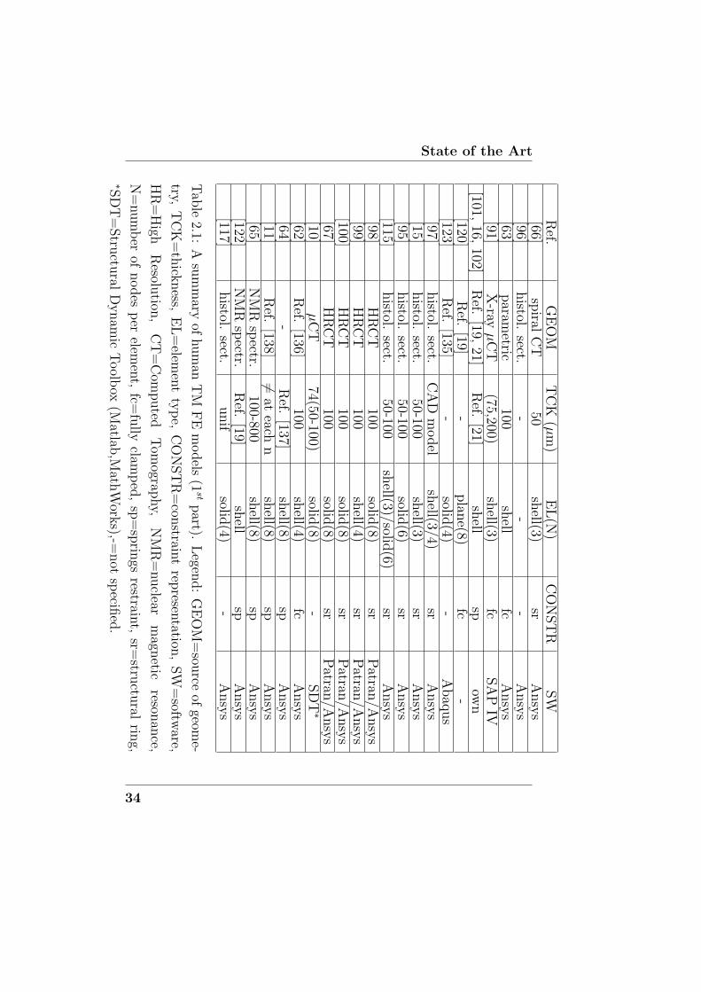
2.3.1 Tympanic membrane modeling
A wide variety of TM FE models can be found in the literature,
differing for geometry, mesh/element, boundary condition and ma-
terial properties. A survey of model main features is reported in this
section and next ones and collected in Tab. 2.1 and Tab. 2.2.
Geometry
Sources
Concerning the source of a geometric model of the anatomy of
the human and animal TM to be used in FE analysis, many in vivo
and in vitro solutions have been proposed [9, 14]. The geometry of
the TM can be based on:
- a simplified parametric geometry (e.g. in terms of a conven-
tionally defined radius of curvature) [90, 107, 62, 63];
- previously published anatomic measurement data [120, 64, 11,
16, 101, 102, 123];
- a 3D reconstruction from serial histological sections [108, 96,
97, 15, 115, 95, 116, 94, 117];
- interferometric techniques (i.e. phase-shift Moir shape mea-
surement) [110, 109, 113, 112, 111, 33, 34, 37, 139];
- nuclear magnetic resonance (NMR) spectroscopy [65, 122];
- micro-Computed Tomography (CT) [91, 114, 10];
33
State of the ArtR
ef.G
EO
MT
CK
(µm
)E
L(N
)C
ON
ST
RSW
[66]sp
iralC
T50
shell(3)
srA
nsy
s[96]
histol.
sect.-
--
Ansy
s[63]
param
etric100
shell
fcA
nsy
s[91]
X-ray
µC
T(75,200)
shell(3)
fcSA
PIV
[101,16,
102]R
ef.[19,
21]R
ef.[21]
shell
spow
n[120]
Ref.
[19]-
plan
e(8)fc
-[123]
Ref.
[135]-
solid(4)
-A
baq
us
[97]histol.
sect.C
AD
model
shell(3/4)
srA
nsy
s[15]
histol.
sect.50-100
shell(3)
srA
nsy
s[95]
histol.
sect.50-100
solid(6)
srA
nsy
s[115]
histol.
sect.50-100
shell(3)/solid
(6)sr
Ansy
s[98]
HR
CT
100solid
(8)sr
Patran
/Ansy
s[99]
HR
CT
100sh
ell(4)sr
Patran
/Ansy
s[100]
HR
CT
100solid
(8)sr
Patran
/Ansy
s[67]
HR
CT
100solid
(8)sr
Patran
/Ansy
s[10]
µC
T74(50-100)
solid(8)
-SD
T∗
[62]R
ef.[136]
100sh
ell(4)fc
Ansy
s[64]
-R
ef.[137]
shell(8)
spA
nsy
s[11]
Ref.
[138]6=
ateach
nsh
ell(8)sp
Ansy
s[65]
NM
Rsp
ectr.100-800
shell(8)
spA
nsy
s[122]
NM
Rsp
ectr.R
ef.[19]
shell
spA
nsy
s[117]
histol.
sect.unif
solid(4)
-A
nsy
s
Tab
le2.1:
Asu
mm
aryof
hum
anT
MF
Em
odels
(1st
part).
Legen
d:
GE
OM
=sou
rceof
geome-
try,T
CK
=th
ickness,
EL
=elem
ent
typ
e,C
ON
ST
R=
constrain
trep
resentation
,SW
=softw
are,
HR
=H
ighR
esolution
,C
T=
Com
puted
Tom
ography,
NM
R=
nuclear
magn
eticreson
ance,
N=
num
ber
ofnodes
per
elemen
t,fc=
fully
clamp
ed,
sp=
sprin
gsrestrain
t,sr=
structu
ralrin
g,∗S
DT
=Stru
ctural
Dynam
icT
oolb
ox(M
atlab,M
athW
orks),-=
not
specifi
ed.
34
ii
“PhDThesis” — 2012/3/26 — 19:36 — page 35 — #21 ii
ii
ii
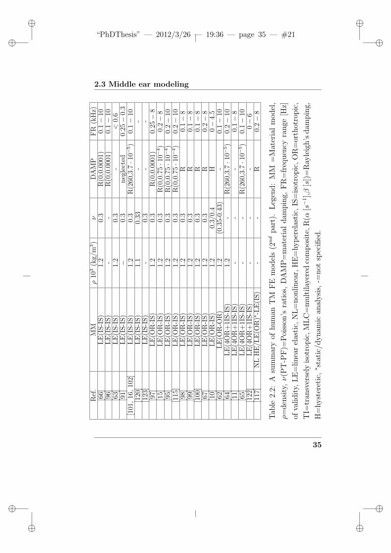
2.3 Middle ear modelingR
ef.
MM
ρ10
3(k
g/m
3)
νD
AM
PF
R(k
Hz)
[66]
LE
(IS-I
S)
1.2
0.3
R(0
,0.0
001)
0.1−
10[9
6]L
E(I
S-I
S)
--
R(0
,0.0
001)
0.1−
10[6
3]L
E(I
S-I
S)
1.2
0.3
-<
0.6
[91]
LE
(IS-I
S)
−0.
3neg
lect
ed0.
25−
0.3
[101
,16
,10
2]L
E(I
S-I
S)
1.2
0.3
R(2
60,3.7·1
0−5)
0.1−
10[1
20]
LE
(IS-I
S)
1.1
0.33
--
[123
]L
E(I
S-I
S)
-0.
3-
-[9
7]L
E(O
R-I
S)
1.2
0.3
R(0
,0.0
001)
0.25−
8[1
5]L
E(O
R-I
S)
1.2
0.3
R(0
,0.7
5·1
0−4)
0.2−
8[9
5]L
E(O
R-I
S)
1.2
0.3
R(0
,0.7
5·1
0−4)
0.2−
10[1
15]
LE
(OR
-IS)
1.2
0.3
R(0
,0.7
5·1
0−4)
0.2−
10[9
8]L
E(O
R-I
S)
1.2
0.3
R0.
1−
8[9
9]L
E(O
R-I
S)
1.2
0.3
R0.
1−
8[1
00]
LE
(OR
-IS)
1.2
0.3
R0.
1−
8[6
7]L
E(O
R-I
S)
1.2
0.3
R0.
2−
8[1
0]L
E(O
R-I
S)
1.2
0.3/
0.4
H0−
4.5
[62]
LE
(OR
-OR
)1.
2(0
.35-
0.43
)-
0.1−
10[6
4]L
E(4
OR
+1I
S-I
S)
1.2
-R
(260
,3.7·1
0−5)
0.2−
10[1
1]L
E(4
OR
+1I
S-I
S)
--
-0.
1−
8[6
5]L
E(4
OR
+1I
S-I
S)
--
R(2
60,3.7·1
0−5)
0.1−
10[1
22]
LE
(4O
R+
1IS-I
S)
--
-0−
6[1
17]
NL
HE
/LE
(OR
)∗-L
E(I
S)
--
R0.
2−
8
Tab
le2.
2:A
sum
mar
yof
hum
anT
MF
Em
odel
s(2nd
par
t).
Leg
end:
MM
=M
ater
ial
model
,
ρ=
den
sity
,ν
(PT
-PF
)=P
oiss
on’s
rati
os,
DA
MP
=m
ater
ial
dam
pin
g,F
R=
freq
uen
cyra
nge
[Hz]
ofva
lidit
y,L
E=
linea
rel
asti
c,N
L=
non
linea
r,H
E=
hyp
erel
asti
c,IS
=is
otro
pic
,O
R=
orth
otro
pic
,
TI=
tran
sver
sely
isot
ropic
,M
LC
=m
ult
ilay
ered
com
pos
ite,
R(α
[s−
1],β
[s])
=R
ayle
igh’s
dam
pin
g,
H=
hyst
eret
ic,∗ s
tati
c/dynam
ican
alysi
s,-=
not
spec
ified
.
35
State of the Art
- spiral CT or High-Resolution Computed Tomography (HRCT)
[66, 98, 99, 100, 118, 119, 67] of living human temporal bones.
Thickness
The human TM thickness is discussed in many works as a critical
parameter with the greatest effects on results. Although there is a
general agreement in considering a non-homogeneous distribution
of thickness in different locations of the TM, a uniform thickness
value, ranging from 30 µm to 150 µm for the human TM is usually
adopted [8, 9, 40, 13, 66]. In [63, 62, 98, 99, 100, 67] a 100 µm value is
assumed, while in other works a different thickness between PT and
PF [91, 65] is considered. Most authors agree to adopt an average
value around 74 µm [8, 15, 26, 35, 32, 14, 31, 10].
The first refinement in thickness representation was made by
[140], who specified 10 thickness regions in their FE model, based
on 10 thickness values measured by [22]. [141, 142, 143] assumed
the same thickness representation for the human TM. Basing on the
same data, [16] constructed a model with a slightly more detailed
thickness distribution of the TM.
It is worth stressing that, according to many authors [40], the
thickness should be related to the Young’s moduli assigned to the
different regions, therefore different combinations of thickness and
elasticity could involve similar results.
Materials
Elastic behavior: models
The question of whether the gross mechanical properties of the
(animal or human) TM are isotropic/anisotropic and uniform or not,
36
ii
“PhDThesis” — 2012/3/26 — 19:36 — page 37 — #22 ii
ii
ii
2.3 Middle ear modeling
have been investigated since the 40’s [27, 28, 19] but it is still difficult
to draw quantitative conclusions about this issue [8].
Mainly linear elastic (LE) models are implemented in the liter-
ature. The viscous behavior of the TM tissues, widely investigated
in recent experimental activities [26, 13, 35], is introduced in the
models as material damping. The main relevant distinction is be-
tween isotropic (IS) and anisotropic (and in particular orthotropic
(OR)) materials. The multi-layer fiber ultrastructure of the PT, sup-
ported by an arrangement of collagen fibers organized into a matrix
of ground substance along radial and circular directions, suggests the
importance of considering the anisotropic material properties of this
sub-membrane; in particular the collagen fiber alignment suggests
the choice for an orthotropic material for the PT. Even if the PF
ultrastructure is composed of distinct layers, the elastic properties
are due to a random distribution of elastin filaments; a regularly and
compactly arranged collagen fiber organization is not present in the
PF [12]. Therefore an homogeneous isotropic material is commonly
assumed for the PF. In the reviewed literature isotropic material
models for both the PT and the PF (with equal or different Young’s
modulus values) have been proposed in [90, 63, 120, 16, 101, 102,
123, 96, 110, 109, 113, 91, 66, 112]. While they both are considered
orthotropic in [62], many studies assume an orthotropic PT and an
isotropic PF, respectively [90, 97, 15, 115, 95, 110, 98, 99, 100, 67, 14].
Other authors [64, 11, 65, 122] implement a 6-part material model
(4 orthotropic and 2 isotropic), shown in Fig. 4.2.
A multilayered orthotropic composite structure of the TM has
been considered in [111, 114]. In [111], since the overall membrane
thickness is considered to taper linearly, the elastic modulus within
37
State of the Art
the fiber layer decreases as 1/r from the umbo to the outer edge.
In [114] distinct models for the radial and circumferential fibrous
layers, as well as two layers corresponding to the combined epider-
mal and subepidermal layers and the mucosal and submucosal layers
are developed. A nominal Young’s modulus of 0.1 GPa is assigned
to both the radial and circumferential fibers so that these fibrous
layers are modeled as transversely isotropic materials, oriented with
the observed fiber directions. Young’s moduli of the radial fibers are
normalized by the local thickness in order to compute a local equiv-
alent modulus for the layer. In the inferior part, the radial fiber
moduli increase as 1/r relatively to the umbo location. The matrix
material and outer layers are assumed to have an isotropic Young’s
modulus of 1 MPa, corresponding to a soft tissue reinforced with
elastin. The PF has an isotropic Young’s modulus of 1 MPa due to
the non-oriented collagen and elastin fibers in the matrix.
Nonlinear hyperelastic models for the TM characterization were
used in [117, 26, 12]. An in-depth study of a TM constitutive model
is described in [117]. A five-parameter hyperelastic Mooney-Rivlin
model for incompressible material is utilized to represent the 3D
constitutive relations of the PT in a quasi-static analysis. Material
properties of the TM and other middle-ear tissues have been mea-
sured by using uniaxial tensile tests. Variations of the mechanical
parameters with stress and in dynamic analysis are also reported in
the same work. An Ogden model was applied to analyze experimen-
tal data obtained with uniaxial tensile, stress relaxation, and failure
tests conducted on fresh human cadaver specimens of the TM in [26].
The Veronda-Westmann hyperelastic model was introduced by [12]
to describe the gerbil PF behavior.
38
ii
“PhDThesis” — 2012/3/26 — 19:36 — page 39 — #23 ii
ii
ii
2.3 Middle ear modeling
Linear elastic parameter values
If an isotropic material model is adopted, Young’s modulus (E)
and Poisson’s ratio (ν) are the usual inputs, while the shear modulus
(G) is obtained by the well-known formula
G =E
2(1 + ν)(2.1)
In the reviewed papers, where isotropy is assumed, Young’s moduli
for human, where not alternatively specified, TM are widely dis-
tributed, as shown in Tab. 2.3, ranging from 1.5 MPa to 20 · 103
MPa for the PT and from 0.5 MPa to 10 · 103 MPa for the PF. In
the isotropic case a 0.5 value of the Poisson’s ratio can be assumed
for incompressible materials while, for a material composed of par-
allel fibers with no lateral interaction among the fibers, Poisson’s
ratio should be considered zero for a stress applied in the direction
of the fibers. A value of 0.3 for the Poisson’s ratio of the TM can be
adopted as a compromise [8].
In most cases an orthotropic model is assumed for the PT while
an isotropic one is used for the PF. If an orthotropic material model
is assumed, nine parameters (three Young’s moduli (EX , EY , EZ),
three Poisson’s ratios (νXY , νXZ , νY Z) and three shear moduli (GXY ,
GXZ , GY Z)) must be used as input. In a plane stress element, which
is commonly assumed in TM models, they reduce to four in-plane
parameters: EX , EY , νXY and GXY .
Young’s moduli values for the orthotropic material models adopted
for regions of the human, where not alternatively specified, TM are
reported in Tab. 2.3. Radial and circumferential Young’s moduli
values for plane stress elements are typically adopted, except in [10],
39
State of the Art
where optimized values for the Young’s moduli are obtained (0.9
MPa for the PF, 4 MPa, 1 MPa, and 0.9 MPa in the radial, cir-
cumferential and thickness directions of the PT, respectively) start-
ing from initially assumed orthotropic PT (32-40 MPa radial; 20-40
MPa circumferential) and isotropic PF (11-14 MPa) as guess values
for the parameter identification procedure.
Only few authors debate the shear modulus issue. In [90] the
shear moduli is set to zero, assuming that the radial fibers slide
over one another without interaction, but this assumption is not
supported by experimental evidences. In [30] the shear modulus is
varied from a large value similar to the fiber stiffness to a very soft
value comparable to loose connective tissue or ground substance. In
[10] an initial 93 MPa value and estimated shear moduli of the PT are
reported (0.8 MPa, 0.9 MPa, 9 MPa in the radial, circumferential and
thickness directions respectively) while in [62] a 6.2 MPa value for the
PT and a 8.5 MPa value for the PF are assumed. In [114] this issue is
extremely debated as a key parameter connected to microstructural
details of the TM; a 35 MPa value of the shear modulus is mentioned,
in order to fit experimental observations.
It is worth noting that, in the orthotropic case, even if Pois-
son’s ratios may be specified in two formulations, denoted major
and minor forms, related through the corresponding Young’s mod-
ulus values, it is not always specified which convention has been
adopted. In the reviewed works, there is a general agreement on
setting a 0.3 value for the human and animal TM Poisson’s ratio
[90, 107, 63, 16, 101, 102, 123, 97, 15, 115, 95, 94, 110, 91, 66, 98,
99, 100, 118, 119, 67, 14, 8, 112, 17] as for the isotropic case and
on the lack of relevant experimental data, even if motivation of this
40
ii
“PhDThesis” — 2012/3/26 — 19:36 — page 41 — #24 ii
ii
ii
2.3 Middle ear modeling
choice represents a controversial issue: some authors consider its in-
fluence negligible on simulation results [90, 8, 63, 97, 91, 14, 9] while
other authors point out the necessity of further investigation on the
influence of varying this parameter in biological material modeling,
proposing other values as zero value [90, 110] or values closer to
0.5 [120, 113, 35, 13, 114, 34] since a 0.5 value [30] (i.e. incompress-
ibility) can cause computational problems. Different values (0.3-0.35
and 0.4-0.43 respectively) for the PT and PF of the TM are reported
in [10, 62].
Material damping
Rayleigh damping is a classical and probably the most common
method to easily build the damping matric C of a numerical model,
under the following form [144]:
C = αM + βK (2.2)
where M and K represent the mass and the stiffness matrix, re-
spectively. Many authors, instead of neglecting damping effects,
introduce material damping in their models in terms of Rayleigh
damping parameters (α [s−1], β [s]) [109, 110, 96, 97, 15, 115, 95,
116, 94, 117, 64, 65, 101, 16, 14, 98, 99, 100, 118, 67, 66]. There is
not a general agreement on α and β values, as shown in Tab. 2.2.
In [114] a complex elastic modulus is used for each component to
model material damping effects. So this simple viscoelastic model
adds an imaginary component to the stiffness that does not increase
with frequency. Hysteretic (or structural) damping is described in
[10].
Density
Many authors agree on setting both the human and animal TM
41
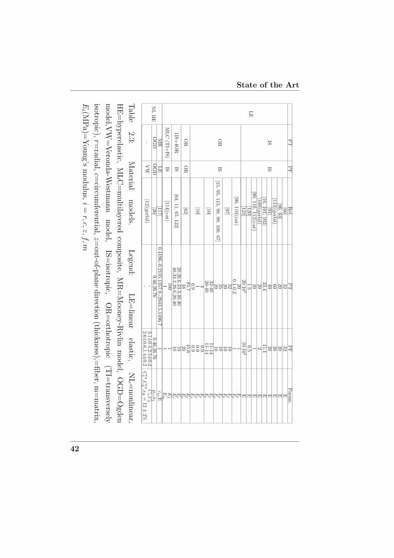
State of the Art
PT
PF
Ref.
PT
PF
Param
.
LE
ISIS
[66]32
32E
[96,63]
2020
E[113](gerb
il)60
20E
[91]40
20E
[16,101,
102]33.4
11.1E
[109](gerbil)
202
E[90,
110,112](cat)
201
E[120]
1.50.5
E[123]
20·103
10·103
E
OR
IS
[90,110](cat)
201
Er
0.1-0.21
Ec
[97]32
10Er
2010
Ec
[15,95,
115,98,
99,100,
67]35
10Er
2010
Ec
[10]32-40
11-14Er
20-4011-14
Er
[10]4
0.9Er
10.9
Ec
0.90.9
Ez
OR
OR
[62]85.7
45.6Er
4820
Ec
1IS+
4OR
IS[64,
11,65,
122]20,26.6,33.3,40,40
10Er
40,33.3,26.6,20,4010
Ec
ML
C(T
I+IS
)IS
[114](cat)100
1Ef
11
Em
NL
HE
MR
LE
[117]0.4196,-0.2135,1357.8,-2843.5,1496.7
1cij ,E
OG
DO
GD
[26]0.46,26.76
0.46,26.76µ
1 ,α1
-V
W[12](gerb
il)-
3.1±0.4,2.5±
0.2C
1 ,C2
-2.6±
0.6,1.4±0.2
CεR
1,C
εR
2,εR
=12±
2%
Tab
le2.3:
Material
models.
Legen
d:
LE
=lin
earelastic,
NL
=non
linear,
HE
=hyp
erelastic,M
LC
=m
ultilayered
comp
osite,M
R=
Moon
ey-R
ivlin
model,
OG
D=
Ogd
en
model,V
W=
Veron
da-W
estman
nm
odel,
IS=
isotropic,
OR
=orth
otropic
(TI=
transversely
isotropic),
r=rad
ial,c=
circum
ferential,
z=ou
t-of-plan
edirection
(thick
ness),=
fib
er,m
=m
atrix,
Ei (M
Pa)=
You
ng’s
modulu
s,i
=r,c,z,f
,m
42
ii
“PhDThesis” — 2012/3/26 — 19:36 — page 43 — #25 ii
ii
ii
2.3 Middle ear modeling
density value to that of water (103 kg/m3) or that of undehydrated
collagen (1.2 · 103 kg/m3) or to values included within this range
[8, 109, 110, 111, 114, 10, 66, 63].
Element type and mesh
Concerning the FE modeling, different element types have been em-
ployed to mesh the animal or human TM geometry [14, 35]:
- (mainly) shell elements [90, 107, 62, 63, 64, 11, 16, 101, 102,
108, 97, 15, 115, 116, 113, 65, 122, 91, 66, 99, 112, 103, 13,
37, 34, 143], eventually thin shell elements combined with thin
beam elements coincident with the common nodes in adjacent
shell elements to represent the fiber structure [121].
- solid (tetrahedral, pentahedral or hexahedral) elements [123,
115, 95, 94, 117, 98, 100, 118, 119, 67, 10], especially in models
accounting for fluid-structure interface between the air (filling
the AC and the middle ear cavity) and the surrounding tissues
modeled as structural parts.
The FE software codes where the mentioned models have been
implemented in, are reported in Tab. 2.1.
Boundary conditions
Constraints
Boundary conditions at the periphery of the TM represent a crit-
ical issue [8]. As previously inferred, the annular ligament (AL) is
the thickened peripheral edge of the PT attached to a groove in an
43
State of the Art
incomplete ring of bone, the cartilagineous tympanic annulus (TA),
which almost encircles it and holds it in place.
Different boundary conditions have been proposed to model the
connection of the TM to the bony wall of the ear canal (Tab. 2.1):
- the periphery of the TM is assumed to be fully clamped (fc)
to the ear canal [90, 8, 107, 112, 62, 63, 120, 113, 91];
- the TA is represented as a structural ring (sr) and in particular
as a linear elastic shell [97, 15, 115] or a solid (pentahedral or
tetrahedral) element structure [115, 95, 94, 100, 118, 67];
- the TM is constrained by linear and torsional springs (sp) in
the longitudinal direction [64, 11, 16, 101, 102, 65, 122]. In
some works, in the spring representation of the TA, due to
the lack of the tympanic ligament in the superior portion of
the TM, the stiffness of the springs in the superior portion is
assumed to be less than that in the inferior portion [16, 101].
The inclusion of the AL or the TA modeled as structural parts,
involves the fact that material parameters are required. Concerning
the material parameters, a linear elastic material model is assumed
for the tympanic AL: a 0.6 MPa values for the Young’s modulus is
adopted in [96, 15, 115, 95, 66] while a 2.5 MPa value in [94] and
a 6 MPa value in [98, 99]. To simulate the flexible support around
the periphery of the TM, the TA was modeled as an elastic ring of
0.2 mm width and 0.2 mm thickness in [97] with a Young’s modulus
initially assumed identical to the radial value for the TM, and then
adjusted as 0.6 MPa through an FE model cross-calibration process.
In [97] the Young’s modulus of the part corresponding to the notch
44
ii
“PhDThesis” — 2012/3/26 — 19:36 — page 45 — #26 ii
ii
ii
2.3 Middle ear modeling
of Rivinus is assumed to be one third of that of the annulus while
the Young’s modulus of the part which divides the TM into PT and
PF, is assumed to have the same Young’s modulus of the PT.
The introduction of spring elements at the periphery of the TM,
involves the assessment of suitable spring constants. In [64] the pe-
riphery of the TM was restrained against radial motion and was
sprung along the longitudinal direction with 34 springs of 75 N/m
stiffness giving a stiffness per unit length of 8.36·104 N/m2. Ansysr
COMBIN14 spring elements are employed in [11]. Spring constant
values are reported in [101, 16]: a 3 ·103 and a 1.5·105 N/m per
unit length value for the superior and the inferior portion respec-
tively for the linear springs; 3·10−5 and 10−4 Nm per unit length for
the superior and the inferior portion respectively for the torsional
springs.
Acoustic loading
A uniform harmonic input pressure stimulus of 80 dB Sound
Pressure Level (SPL) [64, 11, 65, 122, 101, 98, 99, 62] or 90 dB SPL
[91, 96, 15, 95, 117, 10, 123] is frequently applied to the lateral side
of the TM or at the opening of the ear canal, corresponding to a
0.632 Pa value of pressure.
Other values (in the range 80−120 dB SPL corresponding to
0.2 Pa and 20 Pa respectively) [120, 16, 67, 63, 97] are commonly
applied as input sound pressure to the lateral side of the TM or
at the opening of the AC in the numerical and in the experimental
practice.
45
State of the Art
Model assembly: included parts
A critical issue arises in comparing FE results since models can in-
clude different parts of the ear in addition to the TM. Some authors
investigate the behavior of the decoupled TM including sometimes
boundary conditions that mimic the ossicular and eventually inner
ear loading [90, 107, 112].
Several middle ear models in the literature include the ossicles
and sometimes ligaments, tendons and muscles [108, 91, 113, 114,
97, 120, 101, 10, 102, 98, 99, 62, 123, 143, 145].
Complete models (including the air-filled AC and/or the middle
ear cavities and/or the inner ear structures) have been developed in
recent literature [96, 15, 95, 94, 117, 64, 11, 65, 122, 16, 67, 66, 103].
In §4.1, in order to compare different models, the TM has been
considered decoupled from the other parts.
2.3.2 Ossicular chain modeling
Ossicle modeling
In order to simulate the vibratory behavior of the OC, geometric,
inertial and material ossicle data are necessary. In FE analyzes, the
geometry is usually derived by several imaging techniques, mainly:
• ex-vivo micro-computed tomography (µ-CT) scanning of tem-
poral bones e.g. [65, 146];
• scansion and segmentation of histological sections of temporal
bones [104, 96, 97];
46
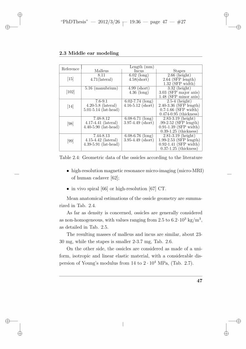
ii
“PhDThesis” — 2012/3/26 — 19:36 — page 47 — #27 ii
ii
ii
2.3 Middle ear modeling
ReferenceLength (mm)
Malleus Incus Stapes
[15]8.11 6.02 (long) 2.66 (height)
4.71(lateral) 4.58(short) 2.64 (SFP length)1.32 (SFP width)
[102]5.16 (manubrium) 4.99 (short) 3.32 (height)
4.36 (long) 3.03 (SFP major axis)1.48 (SFP minor axis)
[14]7.6-9.1 6.02-7.74 (long) 2.5-4 (height)
4.20-5.8 (lateral) 4.16-5.12 (short) 2.40-3.36 (SFP length)5.01-5.14 (lat-head) 0.7-1.66 (SFP width)
0.474-0.95 (thickness)
[98]7.48-8.12 6.08-6.71 (long) 2.83-3.19 (height)
4.17-4.41 (lateral) 3.97-4.49 (short) .99-2.52 (SFP length)4.40-5.90 (lat-head) 0.91-1.39 (SFP width)
0.39-1.25 (thickness)
[99]7.44-8.13 6.08-6.76 (long) 2.81-3.19 (height)
4.15-4.42 (lateral) 3.95-4.49 (short) 1.99-2.53 (SFP length)4.39-5.91 (lat-head) 0.92-1.41 (SFP width)
0.37-1.25 (thickness)
Table 2.4: Geometric data of the ossicles according to the literature
• high-resolution magnetic resonance micro-imaging (micro-MRI)
of human cadaver [62];
• in vivo spiral [66] or high-resolution [67] CT.
Mean anatomical estimations of the ossicle geometry are summa-
rized in Tab. 2.4.
As far as density is concerned, ossicles are generally considered
as non-homogeneous, with values ranging from 2.5 to 6.2 ·103 kg/m3,
as detailed in Tab. 2.5.
The resulting masses of malleus and incus are similar, about 23-
30 mg, while the stapes is smaller 2-3.7 mg, Tab. 2.6.
On the other side, the ossicles are considered as made of a uni-
form, isotropic and linear elastic material, with a considerable dis-
persion of Young’s modulus from 14 to 2 · 104 MPa, (Tab. 2.7).
47
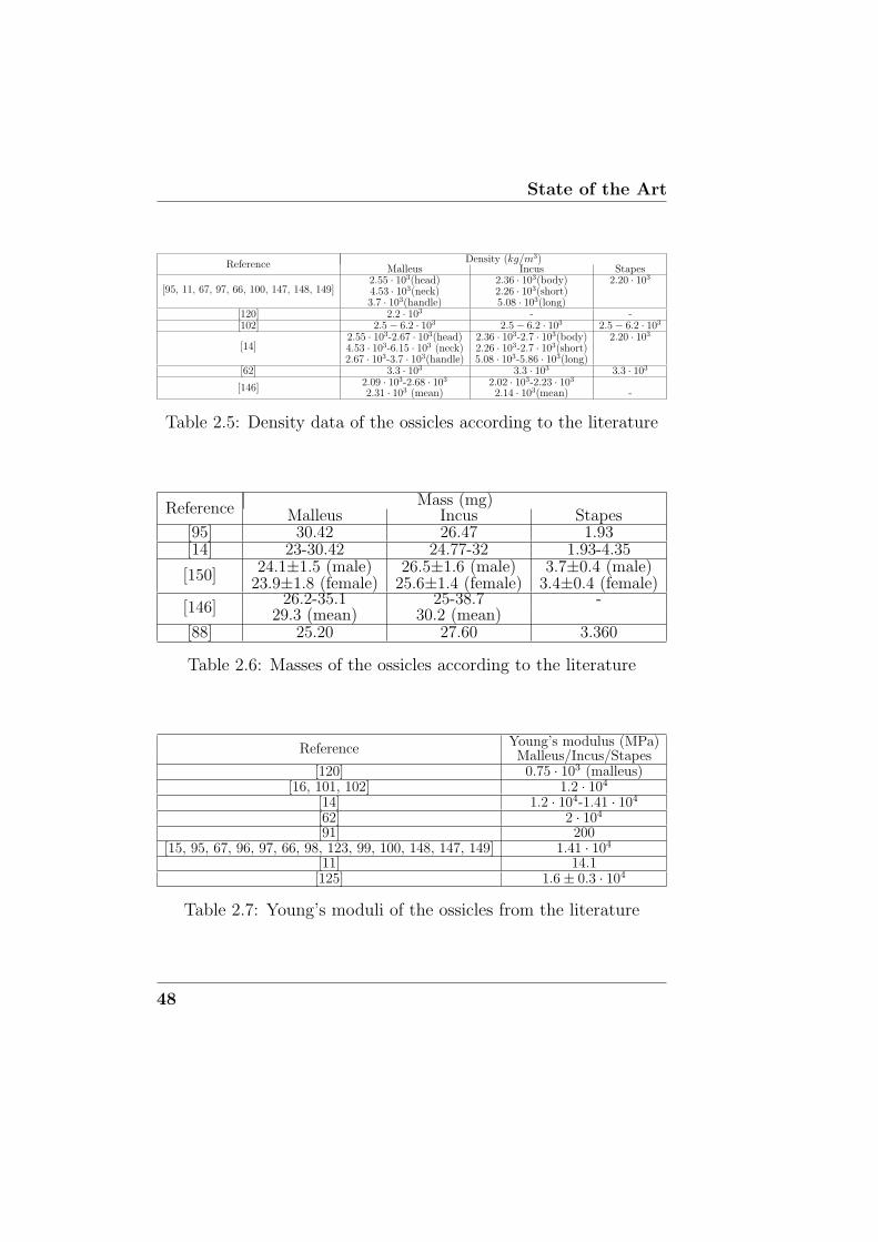
State of the Art
ReferenceDensity (kg/m3)
Malleus Incus Stapes
[95, 11, 67, 97, 66, 100, 147, 148, 149]2.55 · 103(head) 2.36 · 103(body) 2.20 · 103
4.53 · 103(neck) 2.26 · 103(short)3.7 · 103(handle) 5.08 · 103(long)
[120] 2.2 · 103 - -[102] 2.5− 6.2 · 103 2.5− 6.2 · 103 2.5− 6.2 · 103
[14]2.55 · 103-2.67 · 103(head) 2.36 · 103-2.7 · 103(body) 2.20 · 103
4.53 · 103-6.15 · 103 (neck) 2.26 · 103-2.7 · 103(short)2.67 · 103-3.7 · 103(handle) 5.08 · 103-5.86 · 103(long)
[62] 3.3 · 103 3.3 · 103 3.3 · 103
[146]2.09 · 103-2.68 · 103 2.02 · 103-2.23 · 103
2.31 · 103 (mean) 2.14 · 103(mean) -
Table 2.5: Density data of the ossicles according to the literature
ReferenceMass (mg)
Malleus Incus Stapes[95] 30.42 26.47 1.93[14] 23-30.42 24.77-32 1.93-4.35
[150]24.1±1.5 (male) 26.5±1.6 (male) 3.7±0.4 (male)
23.9±1.8 (female) 25.6±1.4 (female) 3.4±0.4 (female)
[146]26.2-35.1 25-38.7 -
29.3 (mean) 30.2 (mean)[88] 25.20 27.60 3.360
Table 2.6: Masses of the ossicles according to the literature
ReferenceYoung’s modulus (MPa)
Malleus/Incus/Stapes[120] 0.75 · 103 (malleus)
[16, 101, 102] 1.2 · 104
[14] 1.2 · 104-1.41 · 104
[62] 2 · 104
[91] 200[15, 95, 67, 96, 97, 66, 98, 123, 99, 100, 148, 147, 149] 1.41 · 104
[11] 14.1[125] 1.6± 0.3 · 104
Table 2.7: Young’s moduli of the ossicles from the literature
48
ii
“PhDThesis” — 2012/3/26 — 19:36 — page 49 — #28 ii
ii
ii
2.3 Middle ear modeling
In the literature, there is a general agreement on assuming a 0.3
value for the Poisson’s ratio for the ossicles, as well as for the other
middle ear components.
In lumped parameters models, the ossicles, considered as rigid
bodies, are characterized by a mass, a center of mass and a principal
inertia tensor. Unfortunately, the inertia tensors and the position of
the centers of mass of the ossicles are rarely reported in the litera-
ture,except in [88, 151, 152].
Because of the complexity of measuring the damping properties
of the middle ear [14], in FE models the damping response of the
ossicles and of the other elements is typically included in terms of
Rayleigh parameters. Typical values are α = 0 s−1 and β = 0.75 ·10−4 s in [15, 95], α = 0 s−1, β = 10−4 s in [97].
Joint modeling
The OC motion depends on the described joints, whose modeling is
complex and crucial. The joints between the malleus and the TM
(TMMJ) and between the stapes and the OW (SOWJ) are fibrous
joints, usually modeled with solid elements; for the TMMJ typical
density and Young’s modulus values are 103 kg/m3 and 4.7 ·103 MPa
while the SOWJ is assumed to be twice as dense and with a wider
dispersion in the elastic constant, 0.065-0.49 MPa.
Structural and functional features that distinguish the synovial
IMJ and ISJ (i.e. the synovial capsules surrounding the articulating
surfaces and the lubricating synovial fluid within those capsules) are
typically reduced in FE models of the middle ear to elastic inter-
faces connecting the articulating surfaces. In particular for the ISJ,
49
State of the Art
a portion of elastic ligamentous tissue is usually interposed between
the two adjacent ossicles, whose characteristics, in terms of density
and Young’s modulus, are 1.2 · 103 kg/m3 and 0.6 MPa respectively
[15, 97]. However, recently two studies on the ISJ modeling were
presented, one on a sub-structured FE model of the cat joint [153],
the other one on an experimentally-calibrated FE model with hyper-
elastic tissue characterization [104].
The disagreement on the role of the IMJ, reported in §1.2.2,
motivated alternative solutions for the modeling of this joint:
• similarly to the ISJ, i.e. as a layer of tissue, but with same
Young’s modulus of the ossicle, therefore acting as a continuous
connection (0 DoFs) between the malleus and the incus [15, 95,
97, 66];
• in [11, 65] it is modeled by linking the malleus and the incus
with stiff three dimensional truss spar elements;
• in [98] a rigid coupling between the FE nodes of the articulating
surfaces is imposed;
• in [73, 87] it is considered as fixed (i.e. allowing no relative
degrees of freedom);
• a two rotational axis (infero-superior and antero-posterior) joint
is assumed in [152];
• in [154] an ideal pin joint scheme is adopted;
• in [123, 155, 148] a contact formulation with a basic Coulomb
friction model is employed;
50
ii
“PhDThesis” — 2012/3/26 — 19:36 — page 51 — #29 ii
ii
ii
2.3 Middle ear modeling
• in [104, 156] it is considered as a standard linear viscoelastic
material with different material parameters (E0 = 40/60 MPa,
E1 = 240/180 MPa, τ1 = 20 µs).
All these references, as well as indications reported in §1.2.2,
allow to infer that the IMJ modeling represents a critical aspect, due
to the wide spread of solutions ranging from 0 (zero) to an effective
6 DoF joint.
In FE models the viscous part of the joint behavior is typically
included in terms of Rayleigh parameters (α = 0 s−1, β = 0.75·10−4 s
[15, 95], α = 0 s−1, β = 5 · 10−4 s [65, 16]. In the lumped parameter
mechanical model of [157], the viscous damping constants for the
joints of the OC are reported within the range 0.001-0.5 Ns/m.
Modeling of other structures
The vibratory behavior of the OC is strongly affected also by the
supporting structures, as ligaments and tendons, which should be
properly modeled.
Commonly, in FE simulations they are included as solid compo-
nents, whose geometry is determined on the basis of imaging tech-
niques [15, 16, 101] or simply assumed as a parallelepiped [65]. Non-
linear hyper-elastic models proved to be suitable to represent the
constitutive relation of ligaments and tendons and in particular of
the ST [81][158], the TT tendon [82], the AML [83] and all of them
[148, 117]. However, due to the reduced amplitude of the vibra-
tory motion, their behavior may be locally approximated by a linear
elastic assumption, e.g. [65, 98]. However, because of the difficul-
ties involved with the experimental measurement of the properties
51
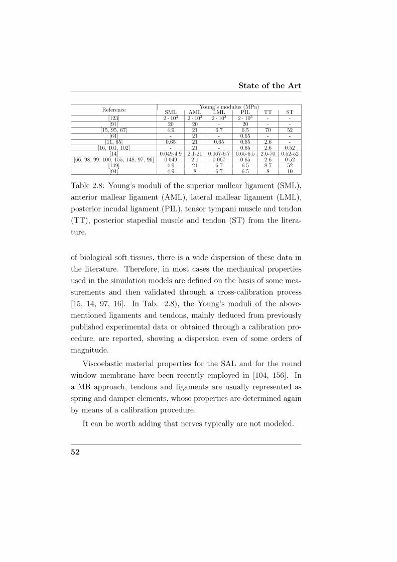
State of the Art
ReferenceYoung’s modulus (MPa)
SML AML LML PIL TT ST[123] 2 · 103 2 · 103 2 · 103 2 · 103 - -[91] 20 20 - 20 - -
[15, 95, 67] 4.9 21 6.7 6.5 70 52[64] - 21 - 0.65 - -
[11, 65] 0.65 21 0.65 0.65 2.6 -[16, 101, 102] - 21 - 0.65 2.6 0.52
[14] 0.049-4.9 2.1-21 0.067-6.7 0.65-6.5 2.6-70 0.52-52[66, 98, 99, 100, 155, 148, 97, 96] 0.049 2.1 0.067 0.65 2.6 0.52
[149] 4.9 21 6.7 6.5 8.7 52[94] 4.9 8 6.7 6.5 8 10
Table 2.8: Young’s moduli of the superior mallear ligament (SML),
anterior mallear ligament (AML), lateral mallear ligament (LML),
posterior incudal ligament (PIL), tensor tympani muscle and tendon
(TT), posterior stapedial muscle and tendon (ST) from the litera-
ture.
of biological soft tissues, there is a wide dispersion of these data in
the literature. Therefore, in most cases the mechanical properties
used in the simulation models are defined on the basis of some mea-
surements and then validated through a cross-calibration process
[15, 14, 97, 16]. In Tab. 2.8), the Young’s moduli of the above-
mentioned ligaments and tendons, mainly deduced from previously
published experimental data or obtained through a calibration pro-
cedure, are reported, showing a dispersion even of some orders of
magnitude.
Viscoelastic material properties for the SAL and for the round
window membrane have been recently employed in [104, 156]. In
a MB approach, tendons and ligaments are usually represented as
spring and damper elements, whose properties are determined again
by means of a calibration procedure.
It can be worth adding that nerves typically are not modeled.
52
ii
“PhDThesis” — 2012/3/26 — 19:36 — page 53 — #30 ii
ii
ii
2.3 Middle ear modeling
End interfaces
In the last years, meaningful advances were made for including the
cochlea in FE models, as an uncoiled [94, 93] or a spiral cochlea [104,
156], for understanding its function and interaction with the middle
ear structures. More frequently, the effect of the cochlear fluid on the
OC is taken into account by means of an equivalent cochlear load,
represented by lumped parameters elements, as viscous dampers [64,
102], viscous dampers with mass [15, 95], spring-dashpot elements
[67, 98] or more complex structures [10].
Such equivalent lumped systems are usually identified in terms
of acoustic input cochlear impedance, defined as the ratio of sound
pressure in the cochlear cavity at the SFP to the volume of fluid the
SFP displaces per unit time (Pa s/m3), whose experimental estima-
tion can be found in the literature, e.g. [159, 160]. A viscous damper
(0.62-0.89 Ns/m) was used by Koike and co-workers [101, 16, 102]
giving a 50 GΩ impedance, deduced from measurements of [160] in
the 0.1 5 kHz frequency range. A similar value (0.717 Ns/m) was also
used in [64], based on a higher estimate of the cochlear impedance (70
GΩ), derived from the stapes displacement measurements reported
in [160]. In [67, 98] a distribution of 49 spring-dashpots elements on
the SFP with constants of 60 N/m and 0.06-0.07 Ns/m, respectively,
was adopted to simulate the action of the cochlear fluids. In [15, 95]
a 20 GΩ cochlear impedance (based on [159, 160]) was obtained as
a mass block of 25.5 mg with 10 dashpots of 0.02 Ns/m, five on each
side of the mass, attached between the SFP and the bony wall. As
far as the TM is concerned, while in the FE models it is almost al-
ways modeled (see [161] for a review), in the lumped parameter or
53
State of the Art
mechanical models it is introduced as a mass element [88, 157] or
omitted [86].
Model inputs and outputs
The kind of input used in the literature can be different, depending
on which parts of the middle ear are modeled. When the AC is
included, the input is a sound stimulus applied at 2 mm away from
the umbo in the ear canal [93] or at the inlet (concha) of the ear
canal [65]. Frequently, when the TM is included, the typical input
is a uniform sound pressure in the 80-120 dB SPL range, applied on
the lateral side of the TM [15].
When only the dynamics of the OC is considered, the displace-
ment of the umbo, as a point of the malleus, in the ”piston-like”
direction, can be assumed as reference input of the model. Although
the TM could transmit also other displacement components to the
malleus, they have been rarely measured [72] and are usually left as
free DoFs.
Another crucial aspect in this kind of simulations is the choice
of the model output, which should be representative of the sound
transmission efficiency and consequently of the vibratory motion of
the ossicles.
The most frequent output in the literature is the SFP displace-
ment amplitude. An alternative representative parameter is the so-
called lever ratio (LR), that is the ratio of the displacement of the
umbo to the displacement of the stapes head, as defined in [76, 16],
or viceversa [11]. The ratio of the umbo displacement to the SFP
displacement is reported in [97, 162]. As stressed in [71, 77], the
54
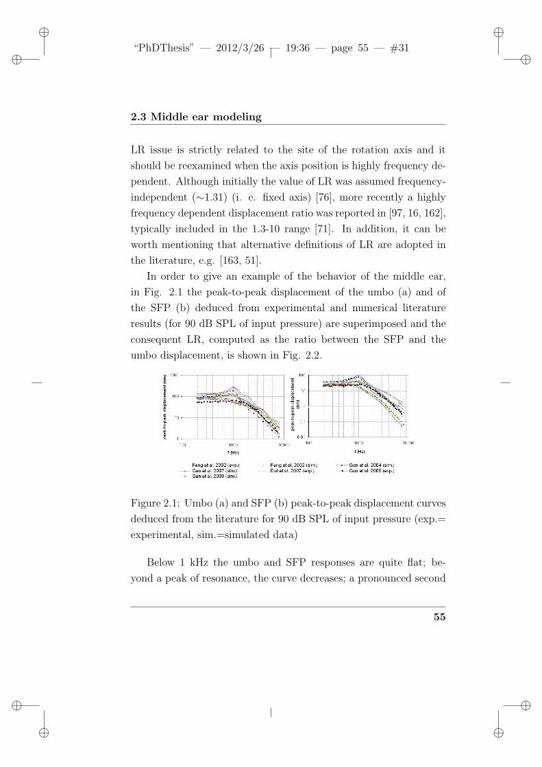
ii
“PhDThesis” — 2012/3/26 — 19:36 — page 55 — #31 ii
ii
ii
2.3 Middle ear modeling
LR issue is strictly related to the site of the rotation axis and it
should be reexamined when the axis position is highly frequency de-
pendent. Although initially the value of LR was assumed frequency-
independent (∼1.31) (i. e. fixed axis) [76], more recently a highly
frequency dependent displacement ratio was reported in [97, 16, 162],
typically included in the 1.3-10 range [71]. In addition, it can be
worth mentioning that alternative definitions of LR are adopted in
the literature, e.g. [163, 51].
In order to give an example of the behavior of the middle ear,
in Fig. 2.1 the peak-to-peak displacement of the umbo (a) and of
the SFP (b) deduced from experimental and numerical literature
results (for 90 dB SPL of input pressure) are superimposed and the
consequent LR, computed as the ratio between the SFP and the
umbo displacement, is shown in Fig. 2.2.
Figure 2.1: Umbo (a) and SFP (b) peak-to-peak displacement curves
deduced from the literature for 90 dB SPL of input pressure (exp.=
experimental, sim.=simulated data)
Below 1 kHz the umbo and SFP responses are quite flat; be-
yond a peak of resonance, the curve decreases; a pronounced second
55
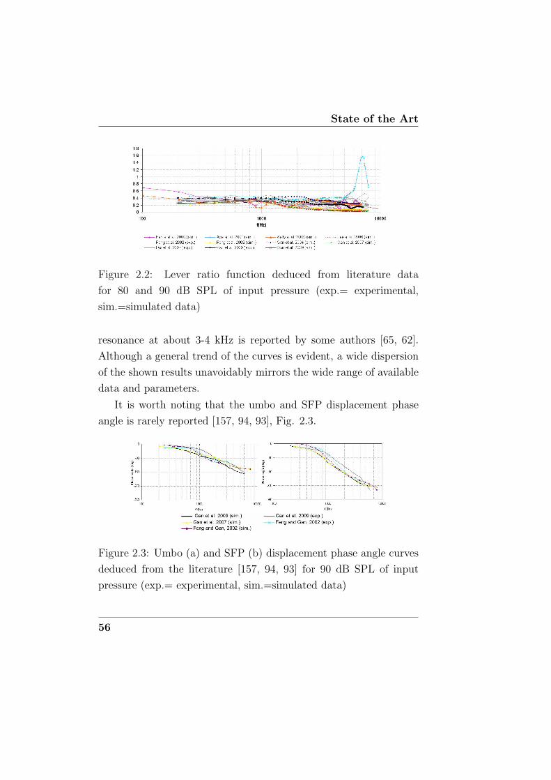
State of the Art
Figure 2.2: Lever ratio function deduced from literature data
for 80 and 90 dB SPL of input pressure (exp.= experimental,
sim.=simulated data)
resonance at about 3-4 kHz is reported by some authors [65, 62].
Although a general trend of the curves is evident, a wide dispersion
of the shown results unavoidably mirrors the wide range of available
data and parameters.
It is worth noting that the umbo and SFP displacement phase
angle is rarely reported [157, 94, 93], Fig. 2.3.
Figure 2.3: Umbo (a) and SFP (b) displacement phase angle curves
deduced from the literature [157, 94, 93] for 90 dB SPL of input
pressure (exp.= experimental, sim.=simulated data)
56
ii
“PhDThesis” — 2012/3/26 — 19:36 — page 57 — #32 ii
ii
ii
2.4 Discussion on the literature survey
It has to be remarked that the OC proved to behave linearly
within the range of input pressure from 80 to 120 dB SPL [97]. Due
to the linearity of the OC in the input range of pressure amplitudes,
the LR vs. frequency trend overlaps for different input pressure levels
as can be ascertained from Fig. 2.2. A significant variability also in
the experimental and numerical LR curves appears, consequent to
uncertainties in experimental measurements (hindered by the scale
of the variables) and in parameter setting, respectively.
It can be worth mentioning that many alternative outputs have
been proposed, e.g. normalized variables such as the displacement
transfer functions of the stapes and of the TM [15] the sound pres-
sure gain or transmission gain/factor [101, 94, 102] and, more gener-
ally, the recorded and monitored pressure at different locations (e.g.
near the OW or round window, ISJ [95] or umbo) inside the mid-
dle ear; the impedance of the middle ear [65]; modal and harmonic
analysis results which are frequently presented in terms of eigenfre-
quencies and displacement distributions [62, 123], velocity plots [94]
and transfer functions [97]; the elliptic trajectories drawn by the tips
of the malleus handle and the stapedial head [16].
2.4 Discussion on the literature survey
2.4.1 Discussion on auditory canal survey
A general agreement on AC modeling arises from the survey. Many
FE models of the human ear include the AC, with a general agree-
ment on materials, element type and boundary conditions.
The geometry of the AC shows relevant inter-subject differences,
57
State of the Art
although a range for a typical human adult subject can be identified.
An accurate study on the AC morphology can help in under-
standing the impact of noise on ears with different AC morpholo-
gies. Moreover, a sensitivity study on size and shape can help in
reconstructive surgery.
2.4.2 Discussion on tympanic membrane survey
On the basis of a survey of the biomechanics of the TM, the relevant
issues about the TM anatomy, structure and available experimental
data have been firstly introduced. Then an overview of modeling
approaches have been presented, mainly focusing on FE model fea-
tures since in the last decades this technique has been extensively
employed in hearing research.
Concerning the experimental characterization of the TM, several
data are available on the geometry and anatomy, thanks to recent
imaging techniques (e.g. µ-CT).
The thickness distribution still represents a critical issue since
only few works in the literature actually measured this parameter in
the human TM. The thickness choice strictly influences the material
properties experimental characterization, since it is typically a priori
assumed in data interpretation. Although some features on relative
thickness distribution in different portions of the TM have been iden-
tified, absolute values of a typical human TM thickness distribution
map are not still available; probably the age-related differences in
thickness or pathologic alterations of available samples hinder the
measurements. Even if histology and ultrastructure of the TM are
deeply detailed by many authors, a standardization of techniques,
58
ii
“PhDThesis” — 2012/3/26 — 19:36 — page 59 — #33 ii
ii
ii
2.4 Discussion on the literature survey
trials and samples with the aim of material characterization does
not yet exist, especially for orthotropic properties identification.
Most recent models still assume a uniform thickness, even if this
parameter is considered highly significant on model results by many
authors.
Another debated issue, highly significant on model outputs, is the
AL constraint representation in the model, due to the complexity to
represent the continuity between the TM fiber thickening, the fibro-
cartilaginous and the bony ring at the periphery of the TM with a
lumped structure.
Despite the available knowledge on TM tissues and fiber arrange-
ment the modeling of these features represents still an argued issue.
The high variability in design choices and modeling parameters,
arising also in the wide range of result values, elucidates the neces-
sity of further and standardized experimental activity for the TM
characterization. Experimental investigations could be oriented to-
wards the characterization of the most significant aspects, also in
order to tune a patient-specific approach.
2.4.3 Discussion on ossicular chain survey
From the analysis of the state of the art concerning the ossicular
chain modeling, reported above, two major issues arise: the wide
dispersion of experimental data, which reflects the remarkable scat-
tering of parameter values in modeling, and the choice of the most
suitable investigation approach.
The dispersion of experimental data, affecting mainly the me-
chanical properties of soft tissues, can be attributed to the difficulties
59
State of the Art
in testing such small elements and to the lack of a standardization
of the experimental procedures. Moreover, although many authors
[162] agree on the good correspondence between the ex vivo and in
vivo measurement of mechanical properties, it is worth noting that
most experimental activity is done on human or animal cadaveric
samples and only few observations on some parts of the middle ear
are done on living human beings [86]. Because of such a dispersion,
parameter values are often tuned through a calibration procedure,
as done in [15, 10, 97]. However, also model calibration are based
on experimental curves, usually the umbo and the SFP displacement
curves (measured with Laser Doppler Vibrometry [97, 93, 116]), that
can markedly differ from author to author and show low repeatability
even within a single experimental session. This can again produce a
wide scattering of the calibrated parameters. It can be worth under-
lying that besides the model calibration procedure, the differences in
displacement amplitudes between the simulated and the experimen-
tal curves are often remarkable, e.g. curves labeled Gan et al. 2009
(exp)/(sim) in Figs. 2.1 and 2.3. Although not much noticeable in
the logarithmic scale, commonly adopted in output presentations,
such differences can be even higher than 100-200%, underlying also
the limits of current models.
As far as investigation approaches are concerned, the FE tech-
nique is employed in the quasi-totality of the recent studies for it
can well represent the highly complex ossicle geometry and the TM
material structure. On the contrary, the extremely simplified repre-
sentation of the articulations certainly is one of the main limitations
of the current FE models of the middle ear and maybe the cause
of the above-mentioned discrepancy between simulated and experi-
60
ii
“PhDThesis” — 2012/3/26 — 19:36 — page 61 — #34 ii
ii
ii
2.4 Discussion on the literature survey
mental curves.
However, other modeling approaches (electro-acoustic or mechan-
ical) are still pursued, because of their simplicity or improvement
in the representation of joints. Till now no direct comparison has
been made between the results of such types of models and the FE
ones. The MB approach certainly involves some drawbacks, for ex-
ample accounting of patient-specific geometries by means of a sim-
plified scheme is not a direct and univocal procedure, while the FE
approach allows a direct import from several imaging techniques
(§2.3.2). However, a sensitivity analysis to geometric parameters is
hindered by a complex geometry with respect to lumped parame-
ters. Besides, the determination of inertia properties which highly
influence the dynamic behavior of the ossicle, is complicated by the
non-homogeneous densities of each ossicle, while in the MB approach
it is simply expressed by means of the mass and inertia tensor [88]
that can be tuned. Concerning material properties, the FE approach
is capable to include viscoelastic and hyperelastic material models,
although the small amplitude of the ossicle vibrations can justify a
linearized analysis.
61

State of the Art
62
ii
“PhDThesis” — 2012/3/26 — 19:36 — page 63 — #35 ii
ii
ii
Chapter 3
Auditory Canal Model
The present chapter focuses on the TM and AC modeling, which are
relevant components in the normal acoustic way and, precisely, in
the outer and middle ear. The TM can be considered as either part
of the outer or middle ear.
The problem was investigated considering two (fluid and struc-
tural) domains for the AC and the TM, respectively, in order to eval-
uate the coupling of different methods and to apply a fluid-structure
interaction (FSI) formulation.
Standard finite element method (FEM) and wave methods, in
particular Generalized Finite Element Method (GFEM), combina-
tion of standard FEM and Partition of Unity Method (PUFEM),
were evaluated and applied, as detailed by the authors in [164]. The
wave methods were selected as suitable to the modeling of sound
propagation at high frequencies.
The analysis results, which include pressure distribution in the
AC and displacement distribution and frequency response of the TM,
63
Auditory Canal Model
confirm experimental and theoretical data proposed in the literature.
The validation of the generalized methods with standard FEM sim-
ulation at increasing mesh density, show the computational advan-
tages of these methods in terms of reduced required mesh density
for a proper accuracy level of results.
3.1 Methods
As reviewed in [165], many physical systems in steady-state oscilla-
tion can be characterized using the Helmholtz equation. The acous-
tic lossless (i.e. viscous dissipation neglected) wave equation for
propagation of sounds in a fluid is given by [133]:
1
c2
∂2P
∂t2−∇2P = 0 (3.1)
where c is the speed of sound in fluid medium, P is the acoustic
pressure, and t represents time. Indicating with f the frequency,
for harmonically varying pressure (i.e. P = P ejωt), where P is the
pressure amplitude and ω = 2πf , Eq. 3.1 reduces to the Helmholtz
equation:ω2
c2P +∇2P = 0 (3.2)
Owing to the requirement of dense spatial discretization, the
modeling of wave fields at high wave numbers is computationally de-
manding when standard, low-order polynomial finite element (FE)
techniques are used. This presents one of the unsolved problems
of the conventional FE method. The incorporation of the physical
features of the solution into the approximation subspace represents
an improvement for relaxing the mesh density of the FEM. This
64
ii
“PhDThesis” — 2012/3/26 — 19:36 — page 65 — #36 ii
ii
ii
3.1 Methods
approach has been utilized for the Helmholtz problem by locally
approximating the solution as a superposition of propagating plane
waves or by enriching the polynomial FE basis function with the
plane waves [165].
The methods proposed in the literature for the high frequency
problems (i.e. when the wave length is lower than or comparable
to the domain size) can be distinguished in Spectral Element Meth-
ods (SEM or SFE), based on Fast Fourier Transform (FFT) [166] or
orthogonal polynomials [167], and Wave Element Methods (WEM)
(e.g. Ultra Weak Variational Formulation, UVWF [165], the Parti-
tion of Unity Method, PUM or PUFEM [168], and the Generalized
Finite Element Method, GFEM [169, 170]).
In the present study, FE models (Ansysr) of the TM and the
AC, in anatomic geometries, Fig. 3.1a, were developed. Moreover,
the GFEM [169] was applied to a simplified geometry of the AC-
TM complex, Fig.3.1b-c. The GFEM method was validated at low
frequency with respect to the FE results.
Figure 3.1: Anatomic (a) and simplified (b,c) auditory canal-
tympanic membrane geometries.
65
Auditory Canal Model
3.1.1 Generalized finite element method (GFEM)
The generalized finite element method (GFEM) is a direct exten-
sion of FEM, which is a special case of GFEM, thus the boundary
conditions can be imposed as in the FEM [169].
The GFEM is a combination of the standard FEM and the par-
tition of unity method (PU(FE)M). The standard polynomial FE
spaces are enriched with special functions (or handbook functions)
reflecting the known information about the boundary value problem.
The special functions are multiplied with the partition of unity cor-
responding to the standard FE linear or bilinear vertex ”hat” shape
functions and are pasted to the FE basis to construct a conforming
approximation [169].
The local approximability is increased due to the handbook func-
tions, while maintaining the existing infrastructures of the FE codes.
In fact, the essential boundary conditions can be imposed in the
GFEM exactly as in the standard FEM [169].
The generalized finite element space Sk,qh,p can be expressed as:
Sk,qh,p =
u|u =
nfem∑k=1
bkNk +nnodes∑j=1
φ∆hi (
q∑j=1
a(i)j W
(i)j )
(3.3)
where Nk denotes the standard bi-p hierarchical FE basis func-
tions defined over the mesh ∆h, p is the standard FE basis function
degree on ∆h, k is the wave number, q is the handbook function
degree at each vertex of ∆h, φ∆hi are the bilinear basis functions cor-
responding to the mesh vertex i, φinnodesi=1 is the partition of unity
employed in the pasting of the handbook functions for the confor-
mity and W (i)j
qj=1 are the handbook functions employed in the ith
66
ii
“PhDThesis” — 2012/3/26 — 19:36 — page 67 — #37 ii
ii
ii
3.1 Methods
vertex. In the PU(FE)M, the first term in the sum in the right-hand
side in Equ. 3.1.1 is not included.
The plane-wave, wave-band and Vekua handbook functions are
evaluated in [170] for the GFEM applied to the Helmholtz problem
solution concluding that they lead to equivalent results, although
the employing of plane-wave functions involves a lower computa-
tional cost and ease of implementation without relevant variations
in asymptotic accuracy for solving the Helmholtz problem, with re-
spect to the more complex functions.
In the present study the plane-wave functions were adopted as
handbook functions W (i)j j=1,....,q; the more general expression is:
W(i)j = eikr (3.4)
In the 2D case the plane wave with direction vector (cos(θj), sin(θj)),
where θj = 2πjq
can be adopted as handbook functions:
W(i)j = e(ik((x−xi) cos θj+(y−yi) sin θj), j = 0, ..., q − 1 (3.5)
In the 3D case, as in the simulation of the fluid domain corre-
sponding to the AC, an extension was required. In the 3D case the
plane waves can be obtained in the following form [171]:
W(i)j = e(ik(x sin θl cosφm+y sin θlsinφm+z cos θl),
θl = lπ
pl = 1, 2, ...p
φm = m2π
qm = 1, 2, ...q
(3.6)
where θl and φm are the angles between the direction of propaga-
tion and two coordinate axes, following the classical spherical polar
67
Auditory Canal Model
convention. Such a direct generalization of the 2D case, where only
one angle is referred, restitutes a distribution of directions which are
concentrated around the poles of an imaginary sphere. As stated in
[171], it is impossible to obtain a perfectly equally-spaced distribu-
tion of directions.
In the below described implementation, the unit vectors of the
propagation directions of the plane-wave functions in the 3D prob-
lems, were selected following the optimized ”spherical covering” logic,
borrowed from another method (e.g. Ultra Weak Variational For-
mulation, UWVF) [165].
The optimized ”spherical covering” logic identifies n points (with
n included in the 4-124 range, Fig. 3.2) on an imaginary sphere,
centered in each mesh node, so that the maximum distance of each
node belonging to the sphere from the nearest of the n considered
points is minimized. Such a criterion allows to obtain a direction
distribution as homogeneous as possible.
In the present study, the same number of directions was assigned
to each node, although an equally-spaced distribution of directions
and an equal number of degrees of freedom at each node are not
required by the method; in fact, a different logic of selection of prop-
agation directions, based on a priori knowledge about the solution,
can allow reducing the number of directions required to obtain a
given accuracy level.
As reported by many authors, an increasing number of wave di-
rections involves a higher result accuracy with the drawback of in-
troducing ill-conditioned system matrices and requiring dedicated
integration techniques. Thus, it is often necessary to introduce in
the implementation some checks on the condition number of the
68
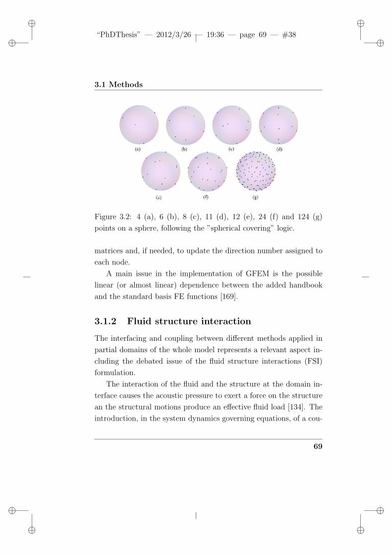
ii
“PhDThesis” — 2012/3/26 — 19:36 — page 69 — #38 ii
ii
ii
3.1 Methods
Figure 3.2: 4 (a), 6 (b), 8 (c), 11 (d), 12 (e), 24 (f) and 124 (g)
points on a sphere, following the ”spherical covering” logic.
matrices and, if needed, to update the direction number assigned to
each node.
A main issue in the implementation of GFEM is the possible
linear (or almost linear) dependence between the added handbook
and the standard basis FE functions [169].
3.1.2 Fluid structure interaction
The interfacing and coupling between different methods applied in
partial domains of the whole model represents a relevant aspect in-
cluding the debated issue of the fluid structure interactions (FSI)
formulation.
The interaction of the fluid and the structure at the domain in-
terface causes the acoustic pressure to exert a force on the structure
an the structural motions produce an effective fluid load [134]. The
introduction, in the system dynamics governing equations, of a cou-
69
Auditory Canal Model
pling matrix accounting for the effective surface area and the normal
to the interface area, represents a possible FSI formulation [134, 133].
In the present study, the FSI coupling formulation described in
[133] was adopted at the interface between fluid and structural do-
mains. Such a formulation involves the building of an asymmetric
element matrix for the interface elements (typically fluid elements),
which have the pressure (pE) and three translational (uE) degrees of
freedom. For the interface fluid element, the structural mass [MS],
damping [CS] and stiffness [KS] matrices, as well as the fluid mass
[MF ], damping [CF ] and stiffness [KF ] matrices, assume the typical
FE form. The total element matrices result:([MS] 0
[MFS] [MF ]
)(uEpE
)+
([CS] 0
0 [CF ]
)(uEpE
)+ (3.7)
+
([KS] [KFS]
0 [KF ]
)(uEpE
)=(FE0
)(3.8)
where [FE] represents the pressure load, [MFS] and [KFS] indicate
the coupling matrices, computed according to the following relations:
[MFS] = ρ0[A]T , [KFS] = −[A] (3.9)
where ρ0 is the fluid density and the coupling matrix [A] is ob-
tained through the following integration on the interface surface S:
[A] =
∫S
NnTN ′TdS (3.10)
where N and N ′ represent the fluid and structural shape
function matrices, respectively. The normal to the interface is indi-
cated with n.
70
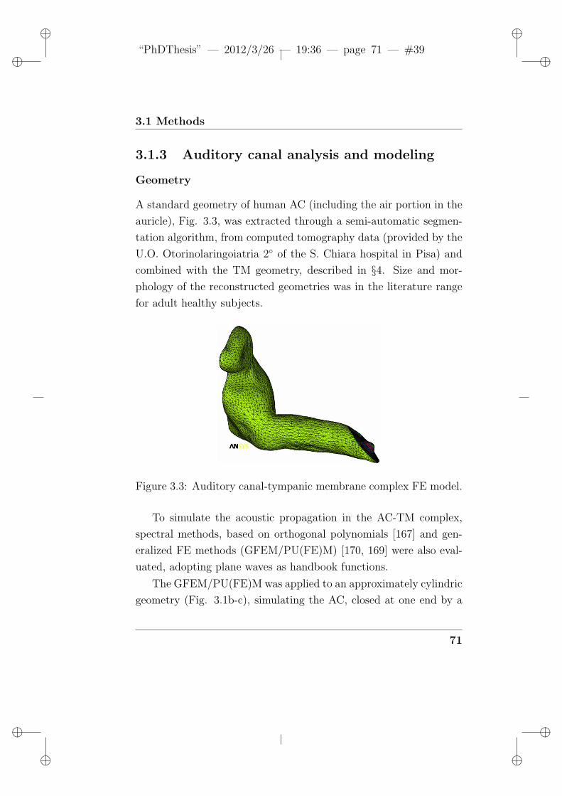
ii
“PhDThesis” — 2012/3/26 — 19:36 — page 71 — #39 ii
ii
ii
3.1 Methods
3.1.3 Auditory canal analysis and modeling
Geometry
A standard geometry of human AC (including the air portion in the
auricle), Fig. 3.3, was extracted through a semi-automatic segmen-
tation algorithm, from computed tomography data (provided by the
U.O. Otorinolaringoiatria 2 of the S. Chiara hospital in Pisa) and
combined with the TM geometry, described in §4. Size and mor-
phology of the reconstructed geometries was in the literature range
for adult healthy subjects.
Figure 3.3: Auditory canal-tympanic membrane complex FE model.
To simulate the acoustic propagation in the AC-TM complex,
spectral methods, based on orthogonal polynomials [167] and gen-
eralized FE methods (GFEM/PU(FE)M) [170, 169] were also eval-
uated, adopting plane waves as handbook functions.
The GFEM/PU(FE)M was applied to an approximately cylindric
geometry (Fig. 3.1b-c), simulating the AC, closed at one end by a
71
Auditory Canal Model
circular membrane, with the aim of facilitate the interface definition.
A fluid-structure interaction formulation (§3.1.2) was employed
between the fluid domain (studied with GFEM/PU(FE)M) and the
structural domain (TM, FEM), with asymmetric matrices.
Materials
The fluid in the AC was assumed as compressible, inviscid, with
uniform mean density and pressure, with the typical values of the
air medium (i.e. a 1.225 kg/m3 density value and a 340 m/s speed
of sound value).
Boundary conditions
The wall of the temporal bone was not included in the model and
replaced by fully clamped boundary conditions at the interface, with
a µ = 0.04 value of adsorption coefficient of the wall.
A pressure load of 90 dB SPL was applied at the inlet of the AC,
corresponding to 0.632 Pa.
Elements
Ansysr 3D acoustic elements (FLUID30) [133, 134] with fluid-structure
interaction and a specific sound absorption coefficient at the inter-
faces with structural parts were employed to mesh the AC volume
in the FE models.
In the present study, a mesh of about 69000 elements and 16000
nodes was adopted for the air in the AC, setting the FSI interaction
for the fluid elements in contact with the TM elements. A coarse
72
ii
“PhDThesis” — 2012/3/26 — 19:36 — page 73 — #40 ii
ii
ii
3.1 Methods
tetrahedral mesh with 224 elements and 94 nodes, was adopted to
test the efficacy of the generalized method with respect to the stan-
dard one.
FE models with an increasing mesh density (i.e. element size
(ESIZE) in the 0.5-4 range, corresponding to a node number between
183 and 8063 and an element number between 611 and 40802) were
developed with the aim of validation of the GFEM models.
3.1.4 Tympanic membrane analysis and model-
ing
Geometry
The anatomic geometry of the TM was obtained as described in the
following (§4), showing typical human adult size and morphology.
The combination of the TM and AC geometries caused size and
shape changes lower than 1%. However, the FE simulation in An-
sysr environment of the decoupled TM was repeated, applying the
pressure load directly on the lateral surface of the membrane to check
the uninfluence of the variations introduced by the image processing
on results.
The circular geometry simulating the TM, adopted in the GFEM
analysis, showed a radius equal to about the average between the
elliptic axes.
Materials, boundary conditions and elements
The materials models reported by [15] were adopted, following an
extended study on the TM, described in §4.
73
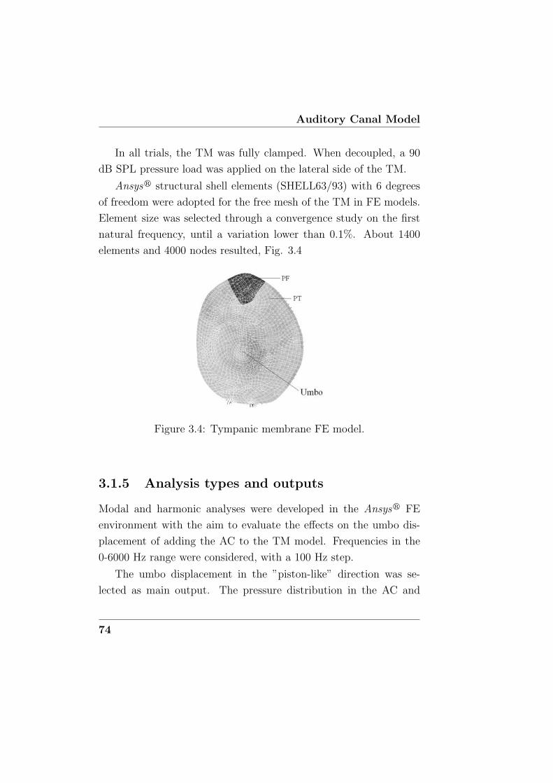
Auditory Canal Model
In all trials, the TM was fully clamped. When decoupled, a 90
dB SPL pressure load was applied on the lateral side of the TM.
Ansysr structural shell elements (SHELL63/93) with 6 degrees
of freedom were adopted for the free mesh of the TM in FE models.
Element size was selected through a convergence study on the first
natural frequency, until a variation lower than 0.1%. About 1400
elements and 4000 nodes resulted, Fig. 3.4
Figure 3.4: Tympanic membrane FE model.
3.1.5 Analysis types and outputs
Modal and harmonic analyses were developed in the Ansysr FE
environment with the aim to evaluate the effects on the umbo dis-
placement of adding the AC to the TM model. Frequencies in the
0-6000 Hz range were considered, with a 100 Hz step.
The umbo displacement in the ”piston-like” direction was se-
lected as main output. The pressure distribution in the AC and
74
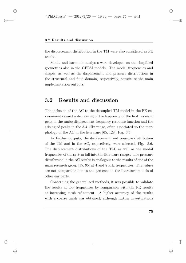
ii
“PhDThesis” — 2012/3/26 — 19:36 — page 75 — #41 ii
ii
ii
3.2 Results and discussion
the displacement distribution in the TM were also considered as FE
results.
Modal and harmonic analyses were developed on the simplified
geometries also in the GFEM models. The modal frequencies and
shapes, as well as the displacement and pressure distributions in
the structural and fluid domain, respectively, constitute the main
implementation outputs.
3.2 Results and discussion
The inclusion of the AC to the decoupled TM model in the FE en-
vironment caused a decreasing of the frequency of the first resonant
peak in the umbo displacement frequency response function and the
arising of peaks in the 3-4 kHz range, often associated to the mor-
phology of the AC in the literature [65, 128], Fig. 3.5.
As further outputs, the displacement and pressure distribution
of the TM and in the AC, respectively, were selected, Fig. 3.6.
The displacement distributions of the TM, as well as the modal
frequencies of the system fall into the literature ranges. The pressure
distribution in the AC results is analogous to the results of one of the
main research group [15, 95] at 4 and 8 kHz frequencies. The values
are not comparable due to the presence in the literature models of
other ear parts.
Concerning the generalized methods, it was possible to validate
the results at low frequencies by comparison with the FE results
at increasing mesh refinement. A higher accuracy of the results
with a coarse mesh was obtained, although further investigations
75
Auditory Canal Model
Figure 3.5: Umbo displacement in the decoupled TM and in the
AC-TM models
are required.
76
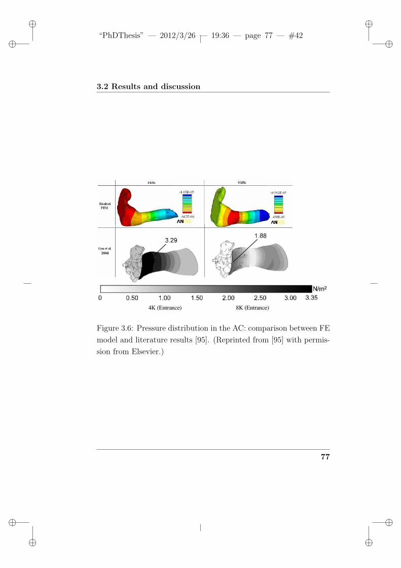
ii
“PhDThesis” — 2012/3/26 — 19:36 — page 77 — #42 ii
ii
ii
3.2 Results and discussion
Figure 3.6: Pressure distribution in the AC: comparison between FE
model and literature results [95]. (Reprinted from [95] with permis-
sion from Elsevier.)
77

Auditory Canal Model
78
ii
“PhDThesis” — 2012/3/26 — 19:36 — page 79 — #43 ii
ii
ii
Chapter 4
Tympanic Membrane Model
The human TM has a key role since it transfers sound waves into
mechanical vibration from the ear canal into the middle ear. The
changes in structure and mechanical properties of the TM due to
middle ear diseases, such as the TM retraction, middle ear infection,
otitis media with effusion, and perforation of the TM, can deteriorate
sound transmission and cause conductive hearing loss [35]. An accu-
rate model of the TM, which directly affects the acoustic-mechanical
transmission, could improve the surgical reconstruction of damaged
eardrums.
FEM is mostly applied to TM modeling for biomedical and clin-
ical purposes. However in literature models with very different fea-
tures (material models/parameters, boundary conditions, element
type, etc.) can be found.
The TM anatomy and a brief summary of experimental investi-
gations employed to characterize the TM mechanical properties and
motion have been previously introduced in §1. Then an overview of
79
Tympanic Membrane Model
modeling approaches was presented in §2, leading to a description of
main features of FE models.
Eight selected reference studies were reproduced for a compar-
ison carried out keeping fixed the TM geometry, except thickness,
and decoupling it from other ear structures included in the original
models. The results of the comparison and of a sensitivity analysis
on one of the reference models are reported in the present chapter
and in [161].
4.1 Comparison of literature finite ele-
ment models
4.1.1 Outline of reference models
In this study, eight reference models, among the many cited, were
selected for a comparison. Each of these models is at least a middle
ear model, including the TM, the ossicular bones (and therefore in-
cudomallear, incudostapedial and tympanostapedial joints) and the
main ligaments.
FE models of the decoupled human TM were created in Ansysr
trying to replicate the characteristics of the selected reference models
in order to elucidate the influence of the main features on simula-
tion results. A summary of the implemented models is reported in
Tab. 4.1 supported by the main references for the design choices.
The models have been sorted in increasing order of material model
complexity. The missing parameters (not specified in the collected
papers) were replaced with the most frequently mentioned values.
80
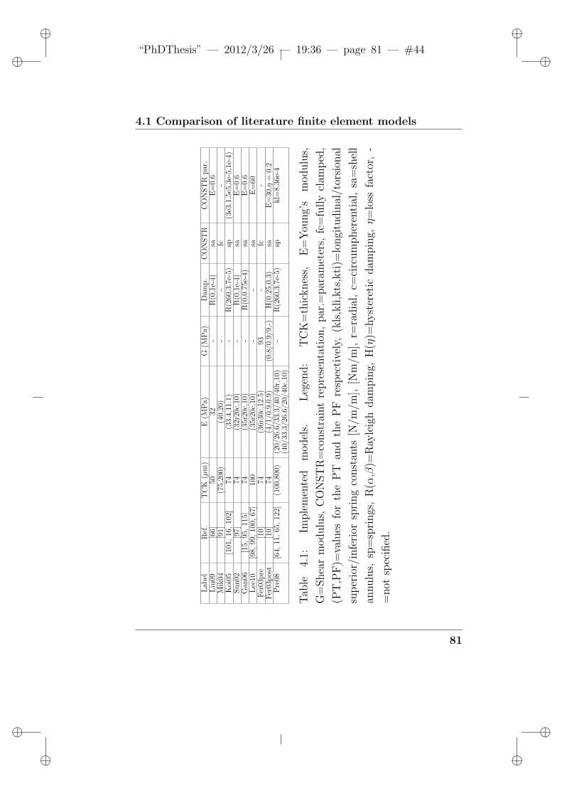
ii
“PhDThesis” — 2012/3/26 — 19:36 — page 81 — #44 ii
ii
ii
4.1 Comparison of literature finite element models
Lab
elR
ef.
TC
K(µ
m)
E(M
Pa)
G(M
Pa)
Dam
p.
CO
NST
RC
ON
ST
Rpar
.L
iu09
[66]
5032
-R
(0,1
e-4)
saE
=0.
6M
ik04
[91]
(75,
200)
(40,
20)
--
fc-
Koi
05[1
01,
16,
102]
74(3
3.4,
11.1
)-
R(2
60,3
.7e-
5)sp
(3e3
,1.5
e5,3
e-5,
1e-4
)Sun02
[97]
74(3
2r20
c,10
)-
R(0
,1e-
4)sa
E=
0.6
Gan
06[1
5,95
,11
5]74
(35r
20c,
10)
-R
(0,0
.75e
-4)
saE
=0.
6L
ee10
[98,
99,
100,
67]
100
(35r
20c,
10)
--
saE
=60
Fer
03pre
[10]
74(3
6r30
c,12
.5)
93-
fc-
Fer
03p
ost
[10]
74(4
/1/0
.9,0
.9)
(0.8
/0.9
/9,-
)H
(0.2
5,0.
3)sa
E=
30,η
=0.
2P
re08
[64,
11,
65,
122]
(100
,800
)(2
0/26
.6/3
3.3/
40/4
0r,1
0)-
R(2
60,3
.7e-
5)sp
kl=
8.36
e-4
(40/
33.3
/26.
6/20
/40c
,10)
Tab
le4.
1:Im
ple
men
ted
model
s.L
egen
d:
TC
K=
thic
knes
s,E
=Y
oung’
sm
odulu
s,
G=
Shea
rm
odulu
s,C
ON
ST
R=
const
rain
tre
pre
senta
tion
,par
.=par
amet
ers,
fc=
fully
clam
ped
,
(PT
,PF
)=va
lues
for
the
PT
and
the
PF
resp
ecti
vely
,(k
ls,k
li,k
ts,k
ti)=
longi
tudin
al/t
orsi
onal
sup
erio
r/in
feri
orsp
ring
const
ants
[N/m
/m],
[Nm
/m],
r=ra
dia
l,c=
circ
um
pher
enti
al,
sa=
shel
l
annulu
s,sp
=sp
rings
,R
(α,β
)=R
ayle
igh
dam
pin
g,H
(η)=
hyst
eret
icdam
pin
g,η=
loss
fact
or,
-
=not
spec
ified
.
81
Tympanic Membrane Model
Liu09
The FE model described in [66] is based on a complete set of CT
images of a living human temporal bone and incorporates the ear
canal, the middle ear suspensory ligaments and muscles, the middle
ear cavity and the inner ear fluid. The TA is included in the model.
A LE IS model, with a uniform thickness of 50 µm, is assumed for
both the PT and the PF of the TM. Fluid-structural interfaces are
defined on the surfaces of acoustic elements next to the movable
structure, such as the TM, ossicles, and suspensory ligaments.
Mik04
Using an x-ray µ-CT of a human temporal bone, a middle ear model
was developed in [91]. A LE IS model is proposed for the TM, with
a uniform thickness of 75 µm and 200 µm for the PT and the PF,
respectively. The TM was fixed around its entire circumference since
the fibrocartilaginous ring not explicitly included in the model.
Koi05
In [101] a 3D FE model of the human middle ear with different depths
of the conical shaped portion of the TM was developed, based on
published data. The model described in [16] (mentioned and used in
[102]) constitutes an improvement of previous models since includes
the ligaments, tendons, middle ear cavities and external auditory
meatus, the damping of the cochlea. More particular aspects, such
as the TM thickness and constraints issues, and the attachment be-
tween the TM and the malleus, are reviewed and enhanced. A LE
82
ii
“PhDThesis” — 2012/3/26 — 19:36 — page 83 — #45 ii
ii
ii
4.1 Comparison of literature finite element models
IS material model is assumed for both the PT and the PF; a not
uniform thickness distribution map was adopted, based on [21]. In
all these studies, the boundary condition at the tympanic ring con-
sists of linear and torsional springs, whose stiffness in the superior
portion is assumed to be less than that in the inferior portion due
to the lack of the tympanic ring in the superior potion.
Sun02
In [97] a geometric model of a human middle ear was constructed in
a CAD environment from histological sections; a working FE model
of the human middle ear was created using previously published
material properties of middle ear components. Six ligaments and
tendons are included and meshed with solid elements. Surrounding
the TM periphery, the TA was modeled using shell elements, with a
thickness assigned in accordance with the TM geometry of the CAD
model. The TM is modeled as a LE shell structure with homoge-
neous and orthotropic material properties; the portion of AL which
divides the eardrum into PT and PF, is assumed to have the same
Young’s modulus as the PT.
Gan06
A 3D finite element model (Fig. 4.1) of the human ear including
the external ear canal, middle ear suspensory ligaments and mus-
cles, and middle ear cavities and cochlear load, constructed based
on a complete set of histological section images of a human tempo-
ral bone is proposed in [15]. The TA was modeled as elastic supports
with shell elements, whose thickness is included in the range 50-100
83
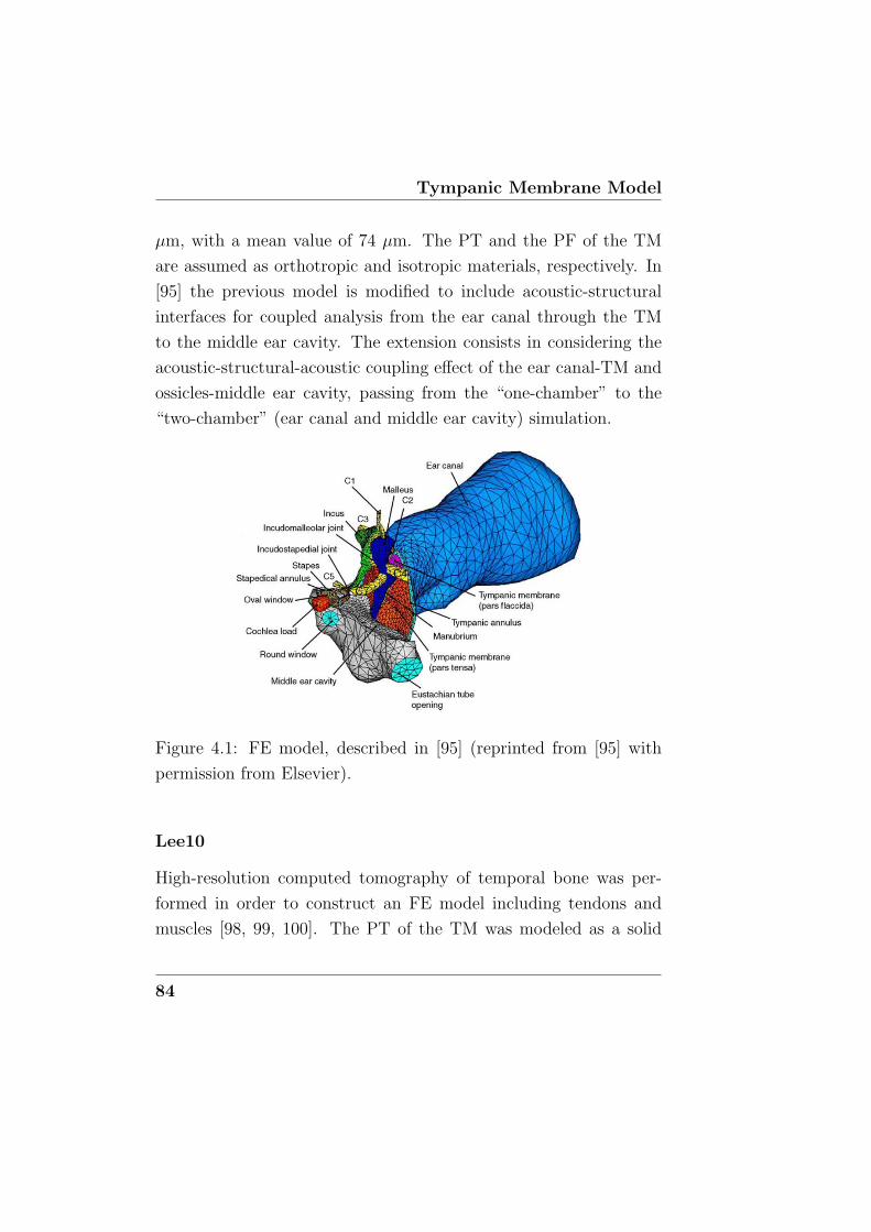
Tympanic Membrane Model
µm, with a mean value of 74 µm. The PT and the PF of the TM
are assumed as orthotropic and isotropic materials, respectively. In
[95] the previous model is modified to include acoustic-structural
interfaces for coupled analysis from the ear canal through the TM
to the middle ear cavity. The extension consists in considering the
acoustic-structural-acoustic coupling effect of the ear canal-TM and
ossicles-middle ear cavity, passing from the “one-chamber” to the
“two-chamber” (ear canal and middle ear cavity) simulation.
Figure 4.1: FE model, described in [95] (reprinted from [95] with
permission from Elsevier).
Lee10
High-resolution computed tomography of temporal bone was per-
formed in order to construct an FE model including tendons and
muscles [98, 99, 100]. The PT of the TM was modeled as a solid
84
ii
“PhDThesis” — 2012/3/26 — 19:36 — page 85 — #46 ii
ii
ii
4.1 Comparison of literature finite element models
element structure with homogenous and orthotropic material prop-
erties, while the PF is assumed isotropic. A uniform thickness of 100
µm was adopted in the model. The periphery of the TM is assumed
to be connected to the bony wall of the ear canal through an elastic
ring.
This model is extended in [67] and a three-chamber (ear canal,
middle ear, and mastoid cavity) FE model of the right ear is devel-
oped, incorporating the external ear canal, middle ear cavity, and
mastoid cavity.
Fer03pre and Fer03post
A mathematical model of the middle ear, based on µ-CT technique
for the geometry importation, is detailed in the dissertation [10].
A relevant aspect of this work relies on the model validation issue,
performed by means of an iterative fitting process in order to iden-
tify the model parameters. As a matter of fact [10] concluded that
the variable conditions and the limitation of the measurement tech-
nique itself certainly affects the efficiency of the fitting procedure
used to identify model parameters, which is strictly dependent on
the number of involved parameters and on the comparison criteria.
Moreover, concerning the physical meaning of the estimated param-
eters, the same author remarks the impossibility to know whether
the identified set of parameter values let a FE model behave like a
mean normal middle ear or like an extremal normal one since slightly
different characteristics and qualities of normal ears exist.
Orthotropic and isotropic material models are assumed for the
PT and the PF respectively and confirmed by the identification pro-
85
Tympanic Membrane Model
cedure. In the model, the TM is considered to be attached to the
sulcus into the bony tympanic ring through the AL, so that the
displacement of the TM at the ring is zero.
A preliminary set of parameters, deduced by [10] from the liter-
ature, and the estimated parameters, resulted from the fitting pro-
cedure, are assumed in the Fer03pre and Fer03post implemented
models, respectively.
Pre08
The 3D FE model described in [64] includes the outer ear canal. A
five part orthotropic PT and an isotropic PF of the TM are assumed;
a varying thickness, taken from [137], was adopted. This model is im-
proved in [11]. An FE model, based on µ-CT and nuclear magnetic
resonance imaging, is developed and employed in [65, 122]. This
model includes the ear canal, five ligaments (the anterior ligament
of the malleus, the lateral ligament of the malleus, the posterior lig-
ament of the incus, the superior ligament of the malleus, and the
superior ligament of the incus) and two muscles (the tensor tympani
muscle and the stapedius muscle). A varying thickness with a max-
imum of 800 µm in the PF and a minimum of 100 µm in the PT
is adopted in [65]. Thickness measurements from [19] are employed
in [122]. In all these works, the periphery of the TM is restrained
against radial motion and springs are employed, along the longitu-
dinal direction, to replicate the flexible connection.
86
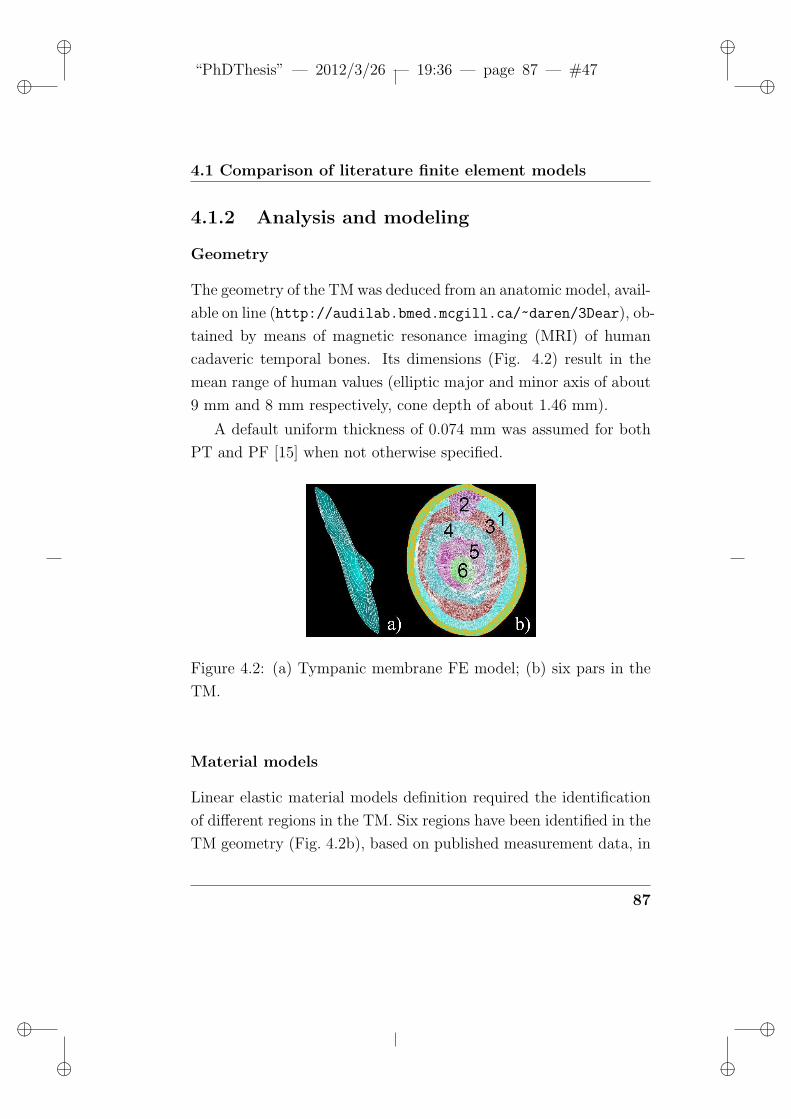
ii
“PhDThesis” — 2012/3/26 — 19:36 — page 87 — #47 ii
ii
ii
4.1 Comparison of literature finite element models
4.1.2 Analysis and modeling
Geometry
The geometry of the TM was deduced from an anatomic model, avail-
able on line (http://audilab.bmed.mcgill.ca/~daren/3Dear), ob-
tained by means of magnetic resonance imaging (MRI) of human
cadaveric temporal bones. Its dimensions (Fig. 4.2) result in the
mean range of human values (elliptic major and minor axis of about
9 mm and 8 mm respectively, cone depth of about 1.46 mm).
A default uniform thickness of 0.074 mm was assumed for both
PT and PF [15] when not otherwise specified.
Figure 4.2: (a) Tympanic membrane FE model; (b) six pars in the
TM.
Material models
Linear elastic material models definition required the identification
of different regions in the TM. Six regions have been identified in the
TM geometry (Fig. 4.2b), based on published measurement data, in
87
Tympanic Membrane Model
order to isolate the PF and distinguish the PT in five zones, as de-
scribed in [64], eventually fused in an homogeneous region depending
on the adopted material model.
Young’s moduli, Poisson’s ratios and densities are required pa-
rameters. In order to include orthotropic properties, local coordinate
systems have been introduced. Since most of the authors refers to
radial and circumferential Young’s moduli, a reference cylindrical co-
ordinate system, centered in the umbo of the TM, was defined. All
element coordinate systems were aligned with the umbo coordinate
system. Shear moduli only appear explicitly in orthotropic models
where they are independent of transverse Young’s moduli. When
required and not alternatively specified, the shear modulus (GXY )
was assumed [172] as
GXY =
√EXEY
2(1 +√
(pxypyx))(4.1)
where EX and EY represent the Young’s moduli in the radial and
circumferential direction respectively, pxy and pyx represent the Pois-
son’s ratio in the major and minor formulation, related by the fol-
lowing
pyx =EYEX
pxy (4.2)
A default 1.2 · 103 kg/m3 density value was assumed in all im-
plemented models except in Fer03post [10] reference model where
a 1.0 · 103 kg/m3 density value was specified.
A default 0.3 Poisson’s ratio value was assumed, except in Fer03pre
[10] (where 0.4 and 0.3 values are specified for the PT and the PF, re-
spectively) and Fer03post [10] reference models (where 0.4/0.1/0.1
88
ii
“PhDThesis” — 2012/3/26 — 19:36 — page 89 — #48 ii
ii
ii
4.1 Comparison of literature finite element models
values in the radial, circumferential and thickness directions are spec-
ified for the PT and a 0.3 value for the PF).
Material damping was included when specified in the reference
study. Mainly Rayleigh damping is employed. α [s−1] and β [s] co-
efficient are reported in Tab. 4.1. Hysteretic damping loss factors η,
assumed in [10], are also reported. The loss factor, used to quan-
tify the level of hysteretic damping of a material, was related to the
damping ratio ζ so viscous damping models were used for analysis.
At resonance it results η = 2ζ.
Boundary conditions
Mainly three constraint representations were implemented in order
to replicate the conditions described in the mentioned works: a fully
clamped periphery, a shell annulus or a spring restraint at the periph-
ery of the TM. It’s worth noting that the choice of considering the
whole TM to be rigidly attached to the tympanic ring around its en-
tire circumference, represents an approximation of the TM anatomy,
since the fibers of the TM extend around the periphery of the PT,
forming the AL, that is a fibrous thickening firmly attached to a sul-
cus in the bony tympanic ring, except superiorly where it separates
the PT from the PF [8].
An annular shell structure, extending around the whole periphery
of the TM and constrained at the outer boundary was introduced
in the models where the presence of the AL was deduced. A 0.22
mm width, a 0.2 mm thickness, a 1.2 ·103 kg/m3 density value and a
0.6 MPa Young’s modulus have been assumed, where not otherwise
specified.
89
Tympanic Membrane Model
As an alternative to directly model the TA, a longitudinal (and
sometimes torsional) spring restraint was adopted when specified in
the corresponding reference model. The TM has been constrained
by means of linear springs in the longitudinal direction (“piston-
like” direction of the ossicles chain and drums) and sometimes also
torsional springs (the Ansysr COMBIN14 element as in [11]). All
other degrees of freedom has been forced to zero displacement and
rotation. Differentiated elastic constants in the inferior or in the
superior portion (representing the “notch of Rivinus”) of the TM
periphery were specified when indicated by the authors. Values of
3.0·103 N/mm and 1.5·105 N/mm for the linear spring constants and
values of 3.0 · 10−5 Nm/m and 10−4 Nm/m for the torsional spring
constants have been assumed for the superior and inferior portion of
the tympanic ring respectively, referring to [101, 16]. Alternatively
the spring constant value was assigned to each spring element con-
sidering a total stiffness per unit length of 8.36 ·104 N/m2 and a TM
radius of 4.8 mm, referring to [64].
Sound pressure stimulus of 90 dB SPL was applied as a uniform
surface load on all elements on the lateral side of the TM.
Mesh, analysis types and outputs
A free quadrilateral mesh (Fig. 4.2) of Ansysr SHELL93/63 ele-
ments was employed in all models. A convergence analysis based on
first undamped natural frequency values was conducted reducing the
mesh size until a variation inferior to 0.1% was obtained. Assuming
this stopping condition, a mesh of 3032 elements and 9027 nodes was
selected.
90
ii
“PhDThesis” — 2012/3/26 — 19:36 — page 91 — #49 ii
ii
ii
4.1 Comparison of literature finite element models
Modal and harmonic analysis were applied in the commercial
FE simulation environment Ansysr. Undamped natural frequen-
cies were recorded as main modal analysis result. The displacement
of the node corresponding to the umbo location, evaluated in the
0−6000 Hz frequency range with a step of 100 Hz, was recorded as
main output of the harmonic analysis.
4.1.3 Results
In this section modal and harmonic analysis results of the imple-
mented models are reported. As already stressed, each model con-
sists in a decoupled TM, since other parts of the ear are not modeled,
and the obtained results can differ from those reported by the orig-
inal authors.
Modal analysis
Modal results in terms of the first twenty undamped natural fre-
quencies for all models are compared in Fig. 4.3; the first three are
reported in Tab. 4.2.
It can be observed that the first natural frequency approximately
results in the 0.9-1.5 kHz range for all models, except for the Fer03post
reference model that gives a 247 kHz value of the first natural fre-
quency. It is interesting to underline that the initial parameter val-
ues, used in Fer03pre, give the highest frequency values in Fig. 4.3,
while values obtained after fitting lead to the lowest ones. A lower
first frequency (about 600-650 kHz) with respect to the mentioned
range results also in Liu09, Sun02, Gan06 reference models, which
91
Tympanic Membrane Model
give very similar values for the first three modal frequencies, despite
the different thickness and material model.
A different combination of parameters results in similar modal
frequencies in Liu09 and Sun02 reference models. The damping
and the boundary conditions at the periphery being equal, a different
material model (IS and homogeneous for the whole TM in the former,
OR in the PT and IS in the PF, and therefore non-homogeneous,
in the latter) and a different thickness result in a similar behaviour
concerning the first twenty resonance frequencies.
As a general observation, a fully clamped or spring restrained
(with the used values of stiffness constants) TM, proposed by Mik04,
Koi05, Fer03pre and Pre08, result in a higher first resonance
frequency with respect to the shell annulus structure proposed by
Liu09, Sun02, Gan06, Lee10 and Fer03post. The next frequen-
cies (Tab. 4.2) show a similar trend and dependence on the param-
eters. However Lee10 model shows several analogies with Mik04,
Fer03pre, Koi05 and Pre08, on the basis of modal results and,
particularly, of the third resonant frequency (Fig. 4.3 and Tab. 4.2);
the high values of the first three resonance frequencies could be re-
lated to the fact that Lee10 model shares a similar constraint, since
the periphery of the TM is constrained by a high-stiffness annulus.
If the modal frequencies are assumed as the most relevant output
of analysis, it appears that a simpler model, as material formulation
and boundary conditions, can be sufficient to reproduce the physio-
logical TM behaviour.
92
ii
“PhDThesis” — 2012/3/26 — 19:36 — page 93 — #50 ii
ii
ii
4.1 Comparison of literature finite element models
Harmonic analysis
Harmonic analysis results of most models of the literature consist in
an umbo displacement frequency response curve, whose features and
values are validated by experimental trials. The results of harmonic
analysis for each implemented model, performed in the 0−6000 Hz
frequency range with a step of 100 Hz are reported in Fig. 4.4.
As already stressed, a wide spread of experimental data is avail-
able in the literature. The obtained values show a good agreement
as order of magnitude and curve trend with respect to the curves
deduced from published results (and overlapped in Fig. 1.6) for
all models, except for Fer03post, for the same reasons reported in
4.1.3. Despite the first resonance is commonly evident in most mod-
els, the TM frequency response at low frequencies does not result
as flat as reported by most authors and the behavior at high fre-
quency shows a lot of variability, confirming the necessity of further
experimental investigations in these frequency ranges, due to their
importance for hearing.
On the basis of harmonic results (Tab. 4.2), analogies can be
found between model behaviors. Considering both resonances and
maximum value of the umbo displacement, Liu09, Sun02 and Gan06
reference models (Fig. 4.4), may form a first group. The Mik04,
Fer03pre, Pre08 and Lee10 reference models can be classified
as a second group, on the basis of the resonance peak frequency.
The Koi05 reference model shows an intermediate behavior between
the two above mentioned groups concerning the first three resonant
peaks frequencies, while the umbo displacement trend and peak am-
plitude are similar to those obtained for Sun02 model. Here again
93
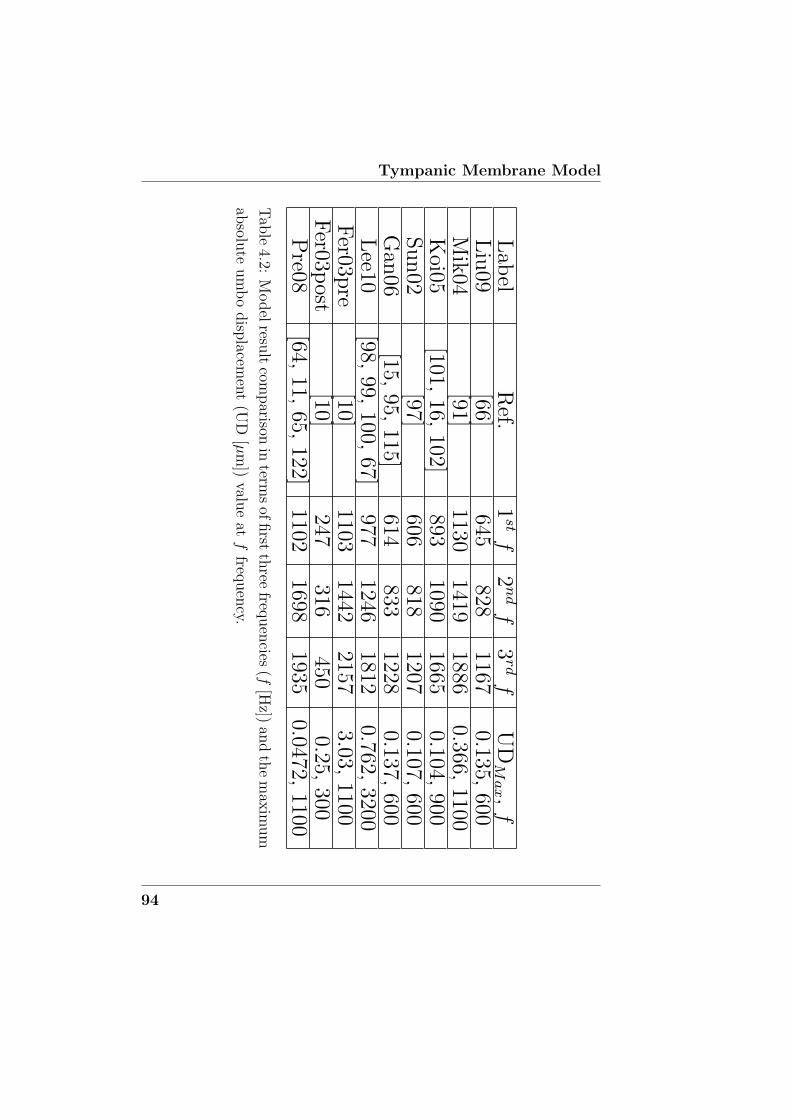
Tympanic Membrane Model
Lab
elR
ef.1stf
2ndf
3rdf
UDMax ,f
Liu
09[66]
645828
11670.135,
600M
ik04
[91]1130
14191886
0.366,1100
Koi05
[101,16,
102]893
10901665
0.104,900
Su
n02
[97]606
8181207
0.107,600
Gan
06[15,
95,115]
614833
12280.137,
600L
ee10[98,
99,100,
67]977
12461812
0.762,3200
Fer03p
re[10]
11031442
21573.03,
1100F
er03post
[10]247
316450
0.25,300
Pre08
[64,11,
65,122]
11021698
19350.0472,
1100
Tab
le4.2:
Model
result
comparison
interm
sof
first
three
frequen
cies(f
[Hz])
and
the
max
imum
absolu
teum
bo
disp
lacemen
t(U
D[µ
m])
value
atf
frequen
cy.
94
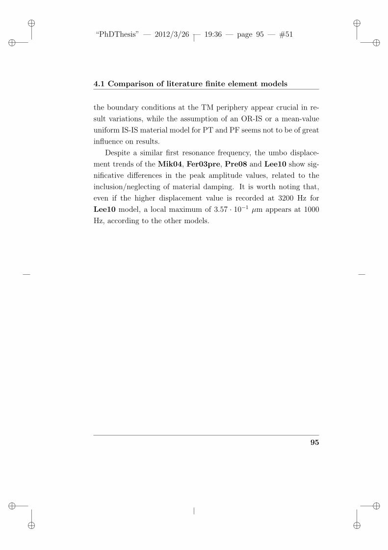
ii
“PhDThesis” — 2012/3/26 — 19:36 — page 95 — #51 ii
ii
ii
4.1 Comparison of literature finite element models
the boundary conditions at the TM periphery appear crucial in re-
sult variations, while the assumption of an OR-IS or a mean-value
uniform IS-IS material model for PT and PF seems not to be of great
influence on results.
Despite a similar first resonance frequency, the umbo displace-
ment trends of the Mik04, Fer03pre, Pre08 and Lee10 show sig-
nificative differences in the peak amplitude values, related to the
inclusion/neglecting of material damping. It is worth noting that,
even if the higher displacement value is recorded at 3200 Hz for
Lee10 model, a local maximum of 3.57 · 10−1 µm appears at 1000
Hz, according to the other models.
95
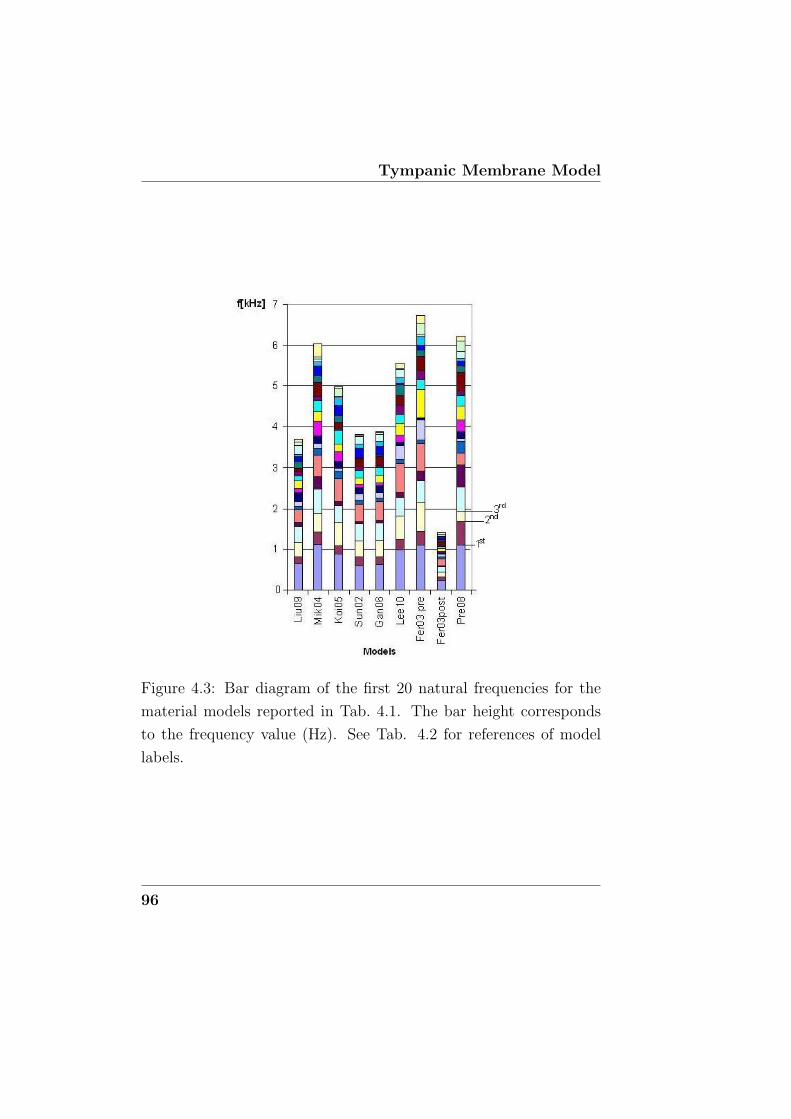
Tympanic Membrane Model
Figure 4.3: Bar diagram of the first 20 natural frequencies for the
material models reported in Tab. 4.1. The bar height corresponds
to the frequency value (Hz). See Tab. 4.2 for references of model
labels.
96
ii
“PhDThesis” — 2012/3/26 — 19:36 — page 97 — #52 ii
ii
ii
4.1 Comparison of literature finite element models
Figure 4.4: Umbo displacement (µm) for the implemented models.
See Tab. 4.2 for references of model labels.
97
Tympanic Membrane Model
4.2 Sensitivity analysis
From the comparison of modal and harmonic results, the model sen-
sitivity to the parameters arises, allowing to infer that the thickness
and the constraint features could be the most influent aspects in TM
modeling, while the complexity of the material model and the choice
of material parameter values appear less influent.
A sensitivity analysis was carried out [173], as a useful tool to
identify the parameters with the highest influence on model results.
A probabilistic approach was adopted, assuming one of the previ-
ously introduced reference models [15, 95] as base model. A uniform
distribution of input parameters was assumes, deducing the param-
eter ranges from the examined literature.
As outputs, the first twenty modal frequencies were analyzed..
4.2.1 Input variables
The input variables consisted of the TM geometric, inertial and ma-
terial parameters. In details, the TM geometry was varied in terms of
size, cone depth and thickness. Size and cone depth variations were
obtained through a radial and a linear scale factor, respectively.
Thicknesses of the PT and PF was varied as independent vari-
ables with a uniform distribution. Concerning the inertial properties,
only the homogeneous density value of the whole TM was varied.
The TM material model was varied in terms of Young’s and shear
modulus, Poisson’s ratio and Rayleigh damping parameters. Dis-
tinct Young’s moduli and Poisson’s ratios for the PT and PF were
considered.
98
ii
“PhDThesis” — 2012/3/26 — 19:36 — page 99 — #53 ii
ii
ii
4.3 Discussion
The influence of the shell annulus, representing the tympanic
annulus and annular ligament which anchor the TM at the periphery,
was evaluated varying its features in terms of geometry (width and
thickness) and material properties (Young’s modulus).
4.2.2 Results
As first result, the statistics of the results were analyzed for varying
of the above mentioned variables in the assigned ranges.
The first modal frequency resulted in the 700-1500 Hz range for
all trials, as widely accepted in the literature.
The most significant parameters consisted of the size scale factor
and density, the thickness and Poisson’s ratio of the PT and the shell
annulus geometry.
Less influent resulted the cone depth scale factor, the PF thick-
ness and the material properties of the PF and shell annulus.
4.3 Discussion
Eight reference models have been compared keeping the geometry
and the loading fixed, and decoupling the TM from other ear struc-
tures included in the original models.
Concerning the critical issues arising in the modeling step, as
previously mentioned in 2, most recent models still assume a uni-
form thickness, even if this parameter is considered highly signifi-
cant on model results by many authors, as confirmed also by some
preliminary trials made by our group in order to better clarify the
importance of lacking or non-specified parameters.
99
Tympanic Membrane Model
Another debated issue, highly significant on model outputs, is
the AL constraint representation in the model. Moreover, despite
the available knowledge on TM tissues and fiber arrangement, the
modeling of these features represents still an argued issue.
The results show that the complexity of the material model and
the choice of material parameter values is less influent with respect
to the constraint representation, as assumed in the a posteriori clas-
sification of reference models based on similar results.
Modal and harmonic results confirmed published assertions on
the TM behavior. From the comparison of results, it can be inferred
that the constraint feature is the most influent feature in TM mod-
eling. However the fundamental importance of the combination of
geometric and material parameters arises from the comparison of the
modal and harmonic results of the implemented models, making the
definition of an optimal model complicated.
Due to the high variability in design choices and modeling param-
eters, a sensitivity analysis is a useful tool to identify the parameters
with the highest influence on model results.
100
ii
“PhDThesis” — 2012/3/26 — 19:36 — page 101 — #54 ii
ii
ii
Chapter 5
Ossicular Chain Model
This chapter is focused on the human middle ear behavior, following
a previous investigation on the AC and the TM [161], described in
§4. From the description of the middle ear anatomical features (§1)
and the detailed model-oriented review of this part (§2) stressing the
most significant assumptions and issues, an original 3D multi-body
(MB) model of the OC is proposed in the present chapter and in
[174].
The MB approach was preferred in this study to the most widespread
finite element method (e.g. [15, 95]), for its main advantage of being
a lumped parameter approach. Thus it simplifies the model elements
definition (body, joints, ligaments etc.) by taking into account only
the characteristics that affect the system dynamic behavior. The
model was used in particular to investigate the debated issue of the
mobility allowed at the incudo-malleolar joint. Simulation results
indicate that such a model achieves a good accuracy, moreover with
a low computational cost.
101
Ossicular Chain Model
5.1 Methods: a multibody model
In order to investigate debated aspects, on the basis of ascertained
data and not including unnecessary assumptions, a simple but ac-
curate 3D lumped parameter model of the OC was developed in the
SimMechanics environment (Matlabr, MathWorks, Massachussetts,
USA).
The model structure was based (although with some significant
modifications) on the doctoral thesis and other studies of T. Wright
[88], while, when available, model parameters were deduced from
[15, 95]. Wright’s model [88] was selected from the literature since he
reported most parameters, allowing reproducing his work; however,
improvements were made in modeling the IMJ and also by including
the LML, the SML and the TT and ST tendons.
It was assumed that the ossicles behave as rigid bodies and that
tissues have a linear visco-elastic response; the synovial joints were
described as smooth ideal mechanical couples. The main elements
of the developed lumped parameter model (shown in Fig. 5.1) are:
• four rigid bodies representing the ossicles (the manubrium and
the head of the malleus are modeled separately) and the lumped
cochlear load mass;
• ideal joints to simulate the IMJ, the ISJ but also the connec-
tions at the ends of the OC (TMMJ and SOWJ);
• spring and damper elements to represent the actions of soft
tissues (tendons, ligaments, joint capsule); in particular six
elements link the ossicles to the ground, representing the AML,
102
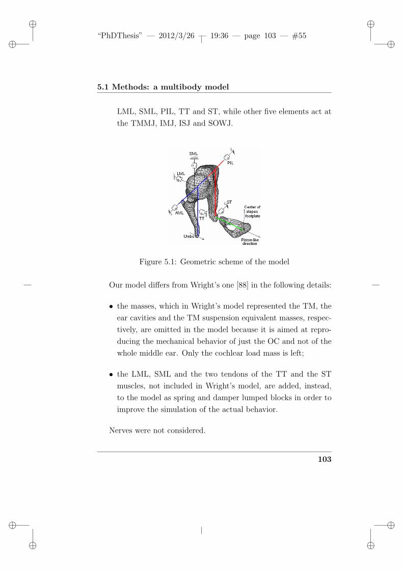
ii
“PhDThesis” — 2012/3/26 — 19:36 — page 103 — #55 ii
ii
ii
5.1 Methods: a multibody model
LML, SML, PIL, TT and ST, while other five elements act at
the TMMJ, IMJ, ISJ and SOWJ.
Figure 5.1: Geometric scheme of the model
Our model differs from Wright’s one [88] in the following details:
• the masses, which in Wright’s model represented the TM, the
ear cavities and the TM suspension equivalent masses, respec-
tively, are omitted in the model because it is aimed at repro-
ducing the mechanical behavior of just the OC and not of the
whole middle ear. Only the cochlear load mass is left;
• the LML, SML and the two tendons of the TT and the ST
muscles, not included in Wright’s model, are added, instead,
to the model as spring and damper lumped blocks in order to
improve the simulation of the actual behavior.
Nerves were not considered.
103
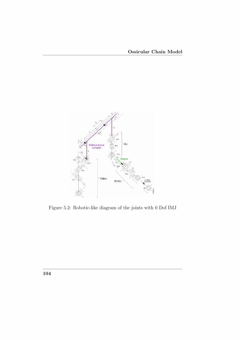
Ossicular Chain Model
Figure 5.2: Robotic-like diagram of the joints with 0 Dof IMJ
104
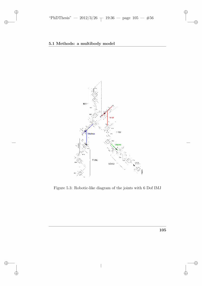
ii
“PhDThesis” — 2012/3/26 — 19:36 — page 105 — #56 ii
ii
ii
5.1 Methods: a multibody model
Figure 5.3: Robotic-like diagram of the joints with 6 Dof IMJ
105
Ossicular Chain Model
In our study two different configurations of the model were de-
veloped, with moveable or fixed IMJ in order to better simulate the
behavior of such a joint.
5.1.1 Basic model geometry
As far as OC geometry is concerned, according to Wright’s model
[88], the main points of the malleus, incus and stapes are indicated
with the letters M , I and S, respectively (Fig. 5.2 and Fig. 5.3).
M1, I1 and S1 denote the centers of mass. M2 denotes the IMJ
(coincident with I2, point on the incus), M3 the point at which the
AML is attached to the malleus, M4 the umbo, considered as the
effective attachment point (umbo) of the manubrium to the TM, I3
the point of attachment of the PIL to the incus, I4 the ISJ location
on the incus, respectively. The ISJ enables a relative motion in both
rotational and translational modes so the location of the joint on
the stapes (denoted as S3) does not in general coincide with I4, ac-
counting for some rotational components around the short and long
axes of the SFP, described in [175]. Unlike in Wright’s model, in our
model the IMJ has relative motion in translation too, according to
experimental evidences in [68, 69]. Point S2 on the stapes coincides
with the geometrical centre of the SFP. Points M4 and S3 are con-
fined to move on parallel lines, in the ”piston-like direction” of the
OC. A γ angle [88] was introduced as a geometric parameter that
represents the inclination defining the AML-PIL ligament axis.
106
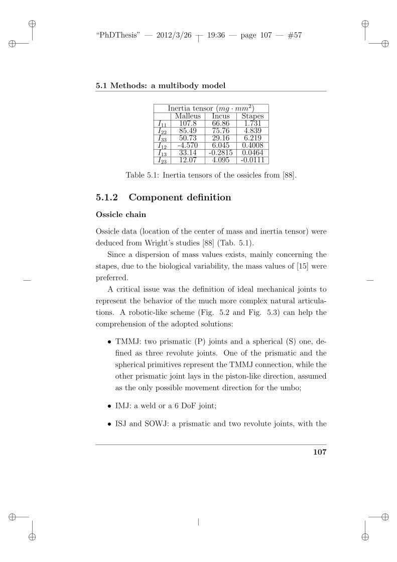
ii
“PhDThesis” — 2012/3/26 — 19:36 — page 107 — #57 ii
ii
ii
5.1 Methods: a multibody model
Inertia tensor (mg ·mm2)Malleus Incus Stapes
I11 107.8 66.86 1.731I22 85.49 75.76 4.839I33 50.73 29.16 6.219I12 -4.570 6.045 0.4008I13 33.14 -0.2815 0.0464I23 12.07 4.095 -0.0111
Table 5.1: Inertia tensors of the ossicles from [88].
5.1.2 Component definition
Ossicle chain
Ossicle data (location of the center of mass and inertia tensor) were
deduced from Wright’s studies [88] (Tab. 5.1).
Since a dispersion of mass values exists, mainly concerning the
stapes, due to the biological variability, the mass values of [15] were
preferred.
A critical issue was the definition of ideal mechanical joints to
represent the behavior of the much more complex natural articula-
tions. A robotic-like scheme (Fig. 5.2 and Fig. 5.3) can help the
comprehension of the adopted solutions:
• TMMJ: two prismatic (P) joints and a spherical (S) one, de-
fined as three revolute joints. One of the prismatic and the
spherical primitives represent the TMMJ connection, while the
other prismatic joint lays in the piston-like direction, assumed
as the only possible movement direction for the umbo;
• IMJ: a weld or a 6 DoF joint;
• ISJ and SOWJ: a prismatic and two revolute joints, with the
107
Ossicular Chain Model
joint axes oriented in the same way;
• a prismatic primitive in the piston-like direction limits the
cochlear load mass movement with respect to the ground.
The prismatic primitive in the IMJ and ISJ allowed a limited
physiological dislocation/ interpenetration of the ossicles in the ar-
ticulation in physiological working conditions, controlled by means
of linear and torsional spring and damper elements. Parameters for
the linear elements, were partially deduced from [157] while an order
of magnitude of the torsional and bending constants were estimated
as initial values to be tuned in an optimization procedure, knowing
the Young’s moduli, the Rayleigh [s] coefficient, an average gap and
the area of contact of each articulation.
Other structures
Spring and damper elements were also introduced to represent lig-
ament (AML, LML, SML, PIL) and tendon (TT, ST) actions, not
included in the robotic-like scheme. The location of the ligaments
and the muscle tendons was estimated from textbooks of anatomy.
Geometric parameters, concerning the ligaments and tendons, ab-
sent in Wright’s model, were deduced from other authors. In partic-
ular, ligaments were assumed 0.8 mm long and 0.5 mm × 0.5 mm.
The TT muscle was taken as 3 mm long and 0.5 mm × 0.5 mm in
cross-section, while the stapedial muscle was taken to be 2 mm long
and 0.43 mm × 0.46 mm in cross-section as in [65, 98]. The mate-
rial properties (Young’s modulus, density) of ligaments and tendons
were mainly deduced from [15, 95]. The Young’s modulus E and
108
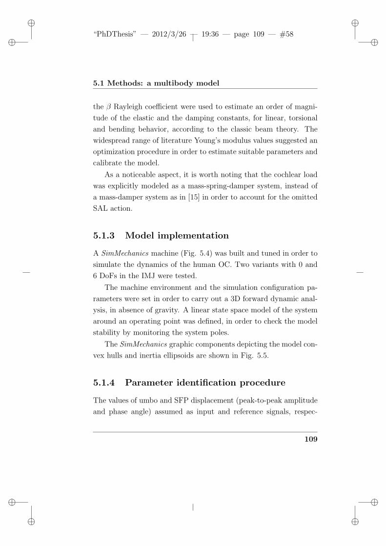
ii
“PhDThesis” — 2012/3/26 — 19:36 — page 109 — #58 ii
ii
ii
5.1 Methods: a multibody model
the β Rayleigh coefficient were used to estimate an order of magni-
tude of the elastic and the damping constants, for linear, torsional
and bending behavior, according to the classic beam theory. The
widespread range of literature Young’s modulus values suggested an
optimization procedure in order to estimate suitable parameters and
calibrate the model.
As a noticeable aspect, it is worth noting that the cochlear load
was explicitly modeled as a mass-spring-damper system, instead of
a mass-damper system as in [15] in order to account for the omitted
SAL action.
5.1.3 Model implementation
A SimMechanics machine (Fig. 5.4) was built and tuned in order to
simulate the dynamics of the human OC. Two variants with 0 and
6 DoFs in the IMJ were tested.
The machine environment and the simulation configuration pa-
rameters were set in order to carry out a 3D forward dynamic anal-
ysis, in absence of gravity. A linear state space model of the system
around an operating point was defined, in order to check the model
stability by monitoring the system poles.
The SimMechanics graphic components depicting the model con-
vex hulls and inertia ellipsoids are shown in Fig. 5.5.
5.1.4 Parameter identification procedure
The values of umbo and SFP displacement (peak-to-peak amplitude
and phase angle) assumed as input and reference signals, respec-
109
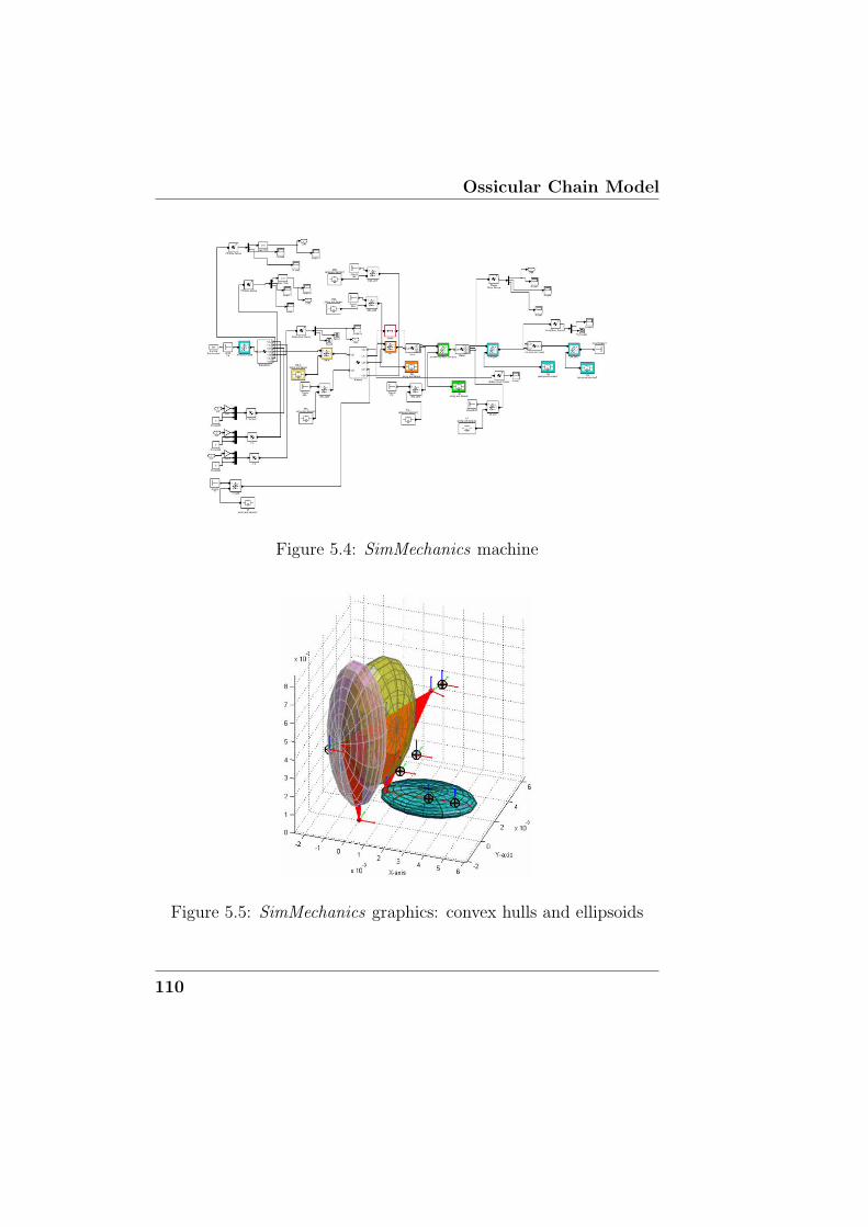
Ossicular Chain Model
Figure 5.4: SimMechanics machine
Figure 5.5: SimMechanics graphics: convex hulls and ellipsoids
110
ii
“PhDThesis” — 2012/3/26 — 19:36 — page 111 — #59 ii
ii
ii
5.1 Methods: a multibody model
tively, for the parameter identification procedure were taken from
published numerical and experimental data [93]. The phase an-
gle values were expressed as phase differences with respect to the
input pressure on the TM, which causes the umbo displacement.
The umbo displacement amplitude and phase angle reference curves
are reported in §2, respectively, with the label Gan et al. 2009
(exp)/(num).
An optimization procedure was developed in order to identify
unspecified parameters but also to tune some parameters whose lit-
erature values range within different orders of magnitude [14], as
done also in [15, 10, 97].
In [15, 97] a cross-calibration procedure based on the minimiza-
tion of the differences between the numerical and experimental SFP
mean peak to peak displacements, in the 250 Hz- 8 kHz range at 90
dB SPL of input pressure at the TM, is employed to derive four un-
determined elastic and damper constants; in [10] an iterative fitting
procedure with 87 parameters, based on trial and error principle and
on a fitting on partial models, is reported.
In this work, as objective function, the sum of the relative errors
between the obtained and the desired SFP displacement amplitude
and phase angle at 58 logarithmically spaced frequencies in the 0.3-6
kHz range was assumed.
The minimization problem was solved in Matlabr by means of
two different optimization approaches: a constrained nonlinear local
and a global (Direct [176]) algorithm. In both cases, lower and upper
boundaries for each variable were defined as 75% of an ascertained
literature or estimated value. In addition, the local minimization
approach required a suitable set of initial values; they were chosen
111
Ossicular Chain Model
from the literature, preferably from [93].
Parameter calibration was carried out to fit the two model ver-
sions (0/6 DoFs at the IMJ) both on numerical (NUM) and experi-
mental (EXP) reference curves, by means of local (LOC) and global
(GLO) optimization algorithms. Moreover, in order to take into ac-
count the higher human sensitivity in the 1-5 kHz frequency range,
the calibration procedure was repeated introducing the A-weighting
curve [5]. Further investigations considered a parameter identifica-
tion based only on the amplitude (and not on the phase angle) and a
double calibration splitting the frequency range in two (<1 kHz, >1
kHz) and considering 58 logarithmically spaced frequencies in each
range.
It is worth noting that the calibration procedure is very complex
due to the high number of parameters to identify and criteria which
must be fulfilled by a set of values, so that the identified set of
parameters must be considered as acceptable and not as the absolute
best set. The choice of the ranges for each parameter is also a critical
issue, since the existence of a set of values out of the boundaries can
not be excluded.
The MB model is characterized by a huge number of geometrical,
inertial and material parameters. In order to reduce the computa-
tional burden of the calibration procedure, only those whose values
were most widespread in the literature, were selected for tuning. A
parameter vector was defined, with 11 and 19 components for the
0/6 DoF IMJ model version, respectively, including the translational
elastic and damping constants of the TMMJ, ISJ (in the piston-like
direction) and of the AML, PIL (in their main line of action), the
damping constants of the ST and SOWJ in the piston-like direction,
112
ii
“PhDThesis” — 2012/3/26 — 19:36 — page 113 — #60 ii
ii
ii
5.1 Methods: a multibody model
the γ angle and, in the 6 DoF IMJ version, all the translational and
rotational elastic and damping constants of the IMJ; for symmetry
in the articulation anatomy, the IMJ constants were assumed equal
in the piston-like and in the vertical directions.
113
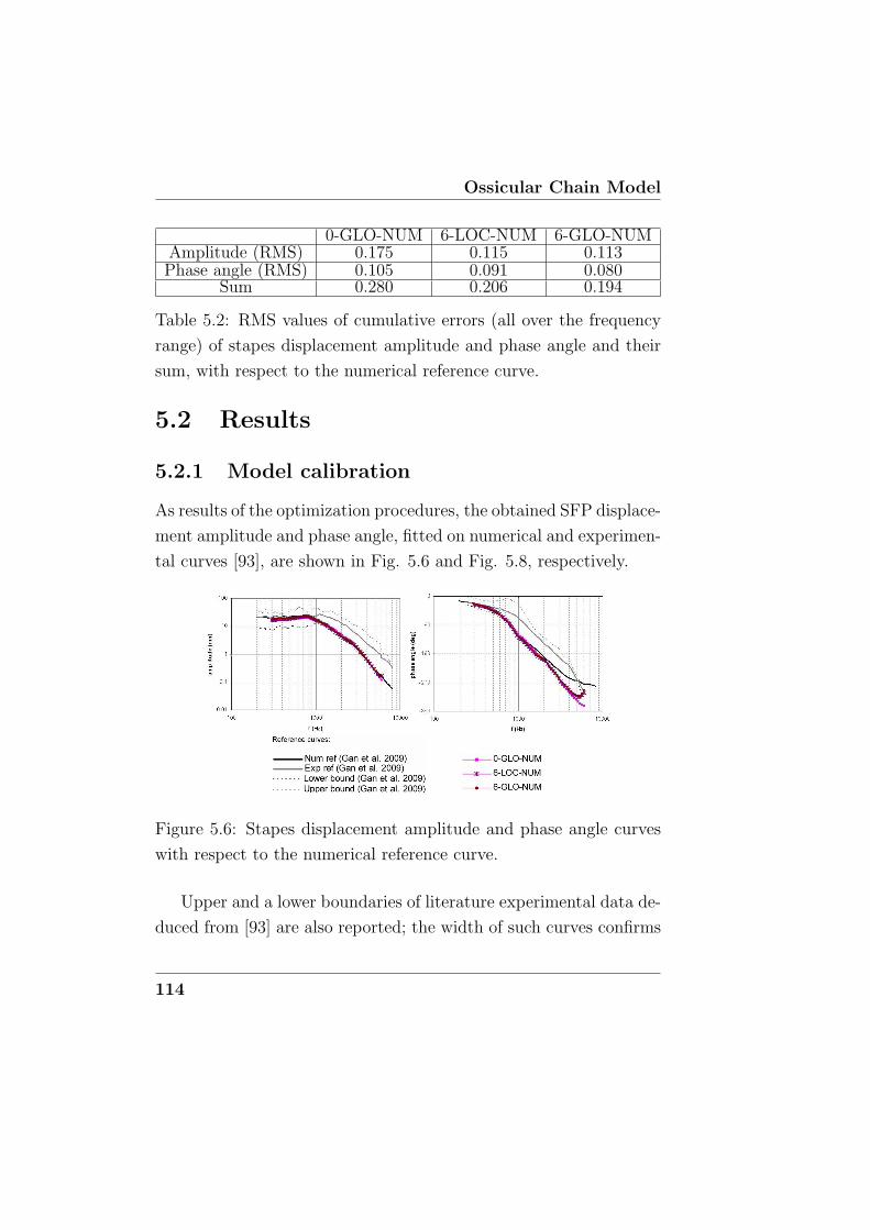
Ossicular Chain Model
0-GLO-NUM 6-LOC-NUM 6-GLO-NUMAmplitude (RMS) 0.175 0.115 0.113Phase angle (RMS) 0.105 0.091 0.080
Sum 0.280 0.206 0.194
Table 5.2: RMS values of cumulative errors (all over the frequency
range) of stapes displacement amplitude and phase angle and their
sum, with respect to the numerical reference curve.
5.2 Results
5.2.1 Model calibration
As results of the optimization procedures, the obtained SFP displace-
ment amplitude and phase angle, fitted on numerical and experimen-
tal curves [93], are shown in Fig. 5.6 and Fig. 5.8, respectively.
Figure 5.6: Stapes displacement amplitude and phase angle curves
with respect to the numerical reference curve.
Upper and a lower boundaries of literature experimental data de-
duced from [93] are also reported; the width of such curves confirms
114
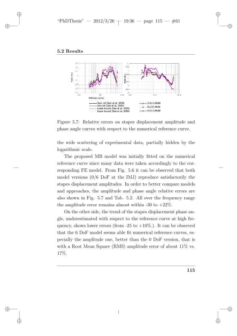
ii
“PhDThesis” — 2012/3/26 — 19:36 — page 115 — #61 ii
ii
ii
5.2 Results
Figure 5.7: Relative errors on stapes displacement amplitude and
phase angle curves with respect to the numerical reference curve.
the wide scattering of experimental data, partially hidden by the
logarithmic scale.
The proposed MB model was initially fitted on the numerical
reference curve since many data were taken accordingly to the cor-
responding FE model. From Fig. 5.6 it can be observed that both
model versions (0/6 DoF at the IMJ) reproduce satisfactorily the
stapes displacement amplitudes. In order to better compare models
and approaches, the amplitude and phase angle relative errors are
also shown in Fig. 5.7 and Tab. 5.2. All over the frequency range
the amplitude error remains almost within -30 to +22%.
On the other side, the trend of the stapes displacement phase an-
gle, underestimated with respect to the reference curve at high fre-
quency, shows lower errors (from -25 to +10%.). It can be observed
that the 6 DoF model seems able fit numerical reference curves, es-
pecially the amplitude one, better than the 0 DoF version, that is
with a Root Mean Square (RMS) amplitude error of about 11% vs.
17%.
115
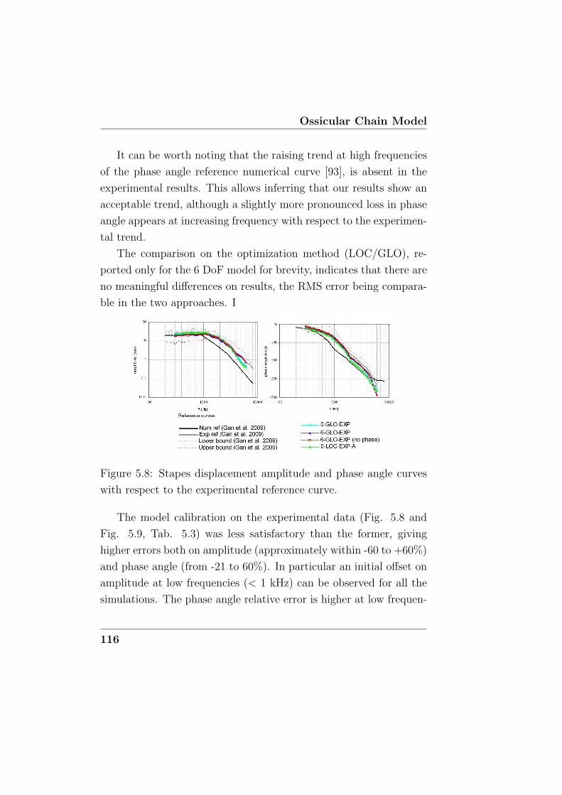
Ossicular Chain Model
It can be worth noting that the raising trend at high frequencies
of the phase angle reference numerical curve [93], is absent in the
experimental results. This allows inferring that our results show an
acceptable trend, although a slightly more pronounced loss in phase
angle appears at increasing frequency with respect to the experimen-
tal trend.
The comparison on the optimization method (LOC/GLO), re-
ported only for the 6 DoF model for brevity, indicates that there are
no meaningful differences on results, the RMS error being compara-
ble in the two approaches. I
Figure 5.8: Stapes displacement amplitude and phase angle curves
with respect to the experimental reference curve.
The model calibration on the experimental data (Fig. 5.8 and
Fig. 5.9, Tab. 5.3) was less satisfactory than the former, giving
higher errors both on amplitude (approximately within -60 to +60%)
and phase angle (from -21 to 60%). In particular an initial offset on
amplitude at low frequencies (< 1 kHz) can be observed for all the
simulations. The phase angle relative error is higher at low frequen-
116
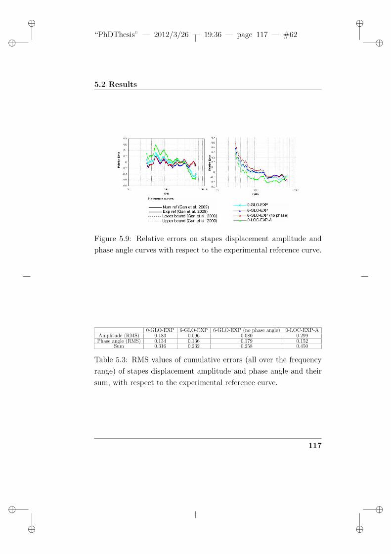
ii
“PhDThesis” — 2012/3/26 — 19:36 — page 117 — #62 ii
ii
ii
5.2 Results
Figure 5.9: Relative errors on stapes displacement amplitude and
phase angle curves with respect to the experimental reference curve.
0-GLO-EXP 6-GLO-EXP 6-GLO-EXP (no phase angle) 0-LOC-EXP-AAmplitude (RMS) 0.183 0.096 0.080 0.299Phase angle (RMS) 0.134 0.136 0.179 0.152
Sum 0.316 0.232 0.258 0.450
Table 5.3: RMS values of cumulative errors (all over the frequency
range) of stapes displacement amplitude and phase angle and their
sum, with respect to the experimental reference curve.
117
Ossicular Chain Model
cies, about 0.4-0.6; however it can be observed that this means an
absolute error below 15 deg. Also in this case the 6 DoF-GLO be-
haved better than the others, as confirmed by the RMS error.
Comparing our results with the numerical reference curve, it can
be remarked that the proposed MB model is able to fit the exper-
imental data better than the corresponding FE model described in
[93].
The addition of the A-weighting function for the calibration on
experimental data, increased the RMS errors both on amplitude and
phase angle, mainly at the boundaries of the frequency range, as
expected. The lowest amplitude error (8%) was obviously obtained
neglecting the phase angle error in the objective function (6-GLO-
EXP (No Phase)); moreover a limited error on the phase angle,
comparable to the other cases, was obtained.
Since some studies distinguish the behavior of the IMJ as show-
ing 0 or 6 DoF at low (< 1 kHz) or high frequencies (> 1 kHz)
respectively, a double calibration procedure was performed on two
partial ranges (< 1 kHz, > 1 kHz).
Results, reported in Fig. 5.10 and Fig. 5.11, indicate that the
calibration on limited ranges is more satisfactory, as confirmed by
the lower RMS errors (Tab. 5.4). While at low frequency (< 1 kHz)
both the 0 and the 6 DoF models gave similar results, above 1 kHz
the latter was able to better fit the experimental curve, giving a lower
error (0.16 vs. 0.294) particularly on amplitude (0.093 vs. 0.199).
The parameter values obtained for the 6-GLO-EXP, fitted on the
whole range and on the restricted ranges (< 1 kHz, > 1 kHz) cases,
are reported, as an example, in Tab. 5.5.
All identified parameters fall strictly within the assigned ranges
118
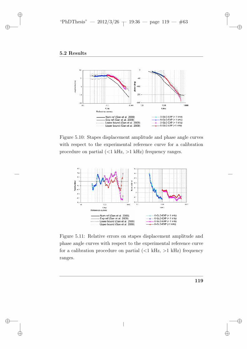
ii
“PhDThesis” — 2012/3/26 — 19:36 — page 119 — #63 ii
ii
ii
5.2 Results
Figure 5.10: Stapes displacement amplitude and phase angle curves
with respect to the experimental reference curve for a calibration
procedure on partial (<1 kHz, >1 kHz) frequency ranges.
Figure 5.11: Relative errors on stapes displacement amplitude and
phase angle curves with respect to the experimental reference curve
for a calibration procedure on partial (<1 kHz, >1 kHz) frequency
ranges.
119
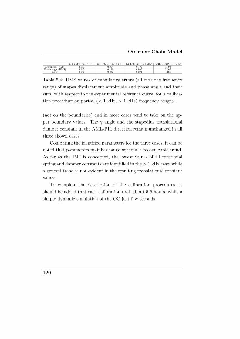
Ossicular Chain Model
0-GLO-EXP (< 1 kHz) 6-GLO-EXP (< 1 kHz) 0-GLO-EXP (> 1 kHz) 6-GLO-EXP (> 1 kHz)Amplitude (RMS) 0.097 0.094 0.199 0.093Phase angle (RMS) 0.145 0.138 0.095 0.067
Sum 0.242 0.232 0.294 0.160
Table 5.4: RMS values of cumulative errors (all over the frequency
range) of stapes displacement amplitude and phase angle and their
sum, with respect to the experimental reference curve, for a calibra-
tion procedure on partial (< 1 kHz, > 1 kHz) frequency ranges..
(not on the boundaries) and in most cases tend to take on the up-
per boundary values. The γ angle and the stapedius translational
damper constant in the AML-PIL direction remain unchanged in all
three shown cases.
Comparing the identified parameters for the three cases, it can be
noted that parameters mainly change without a recognizable trend.
As far as the IMJ is concerned, the lowest values of all rotational
spring and damper constants are identified in the > 1 kHz case, while
a general trend is not evident in the resulting translational constant
values.
To complete the description of the calibration procedures, it
should be added that each calibration took about 5-6 hours, while a
simple dynamic simulation of the OC just few seconds.
120
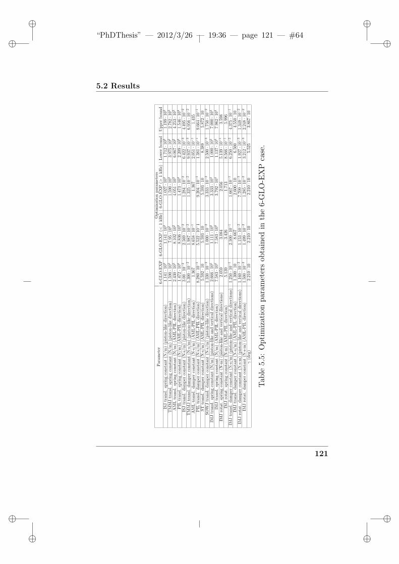
ii
“PhDThesis” — 2012/3/26 — 19:36 — page 121 — #64 ii
ii
ii
5.2 Results
Par
amet
erO
pti
miz
atio
npar
amet
ers
6-G
LO
-EX
P6-
GL
O-E
XP
(<1
kH
z)6-
GL
O-E
XP
(>1
kH
z)L
ower
bou
nd
Upp
erb
ound
ISJ
tran
sl.
spri
ng
const
ant
(N/m
)(p
isto
n-l
ike
dir
ecti
on)
1.14
1·1
031.
141·1
031.
027·1
031.
712·1
021.
199·1
03
TM
MJ
tran
sl.
spri
ng
const
ant
(N/m
)(p
isto
n-l
ike
dir
ecti
on)
1.59
0·1
037.
95·1
021.
590·1
033.
975·1
022.
782·1
03
AM
Ltr
ansl
.sp
ring
const
ant
(N/m
)(A
ML
-PIL
dir
ecti
on)
2.43
0·1
038.
102·1
024.
051·1
036.
067·1
024.
253·1
03
PIL
tran
sl.
spri
ng
const
ant
(N/m
)(A
ML
-PIL
dir
ecti
on)
1.47
2·1
048.
836·1
031.
473·1
042.
209·1
031.
546·1
04
ISJ
tran
sl.
dam
per
const
ant
(N·s/
m)
(pis
ton-l
ike
dir
ecti
on)
3.00·1
0−2
2.56
9·1
0−2
1.28
4·1
0−2
6.42
2·1
0−3
4.49
5·1
0−2
TM
MJ
tran
sl.
dam
per
const
ant
(N·s/
m)
(pis
ton-l
ike
dir
ecti
on)
5.30
0·1
0−2
1.98
7·1
0−2
1.32
5·1
0−2
9.93
7·1
0−3
6.95
6·1
0−2
AM
Ltr
ansl
.dam
per
const
ant
(N·s/
m)
(AM
L-P
ILdir
ecti
on)
1.36
78.
658·1
0−1
1.36
72.
051·1
0−1
1.43
5P
ILtr
ansl
.dam
per
const
ant
(N·s/
m)
(AM
L-P
ILdir
ecti
on)
8.28
0·1
0−1
5.52
2·1
0−1
9.20
4·1
0−1
1.38
1·1
0−1
9.66
4·1
0−1
ST
tran
sl.
dam
per
const
ant
(N·s/
m)
(AM
L-P
ILdir
ecti
on)
5.59
2·1
05.
593·1
05.
593·1
08.
389
5.87
2·1
0SO
WJ
tran
sl.
dam
per
const
ant
(N·s/
m)
(pis
ton-l
ike
dir
ecti
on)
1.33
0·1
0−2
1.00
0·1
0−2
3.33
3·1
0−3
2.50
0·1
0−3
1.75
0·1
0−2
IMJ
tran
sl.
spri
ng
const
ant
(N/m
)(p
isto
n-l
ike
and
vert
ical
dir
ecti
ons)
2.66
6·1
041.
111·1
043.
333·1
041.
000·1
047.
000·1
04
IMJ
tran
sl.
spri
ng
const
ant
(N/m
)(A
ML
-PIL
dir
ecti
on)
7.58
3·1
047.
583·1
043.
792·1
041.
137·1
047.
962·1
04
IMJ
rota
t.sp
ring
const
ant
(N·m
)(p
isto
n-l
ike
and
vert
ical
dir
ecti
ons)
2.05
93.
084
2.05
65.
139·1
0−1
3.59
8IM
Jro
tat.
spri
ng
const
ant
(N·m
)(A
ML
-PIL
dir
ecti
on)
5.13
93.
426
1.71
38.
566·1
0−1
5.99
6IM
Jtr
ansl
.dam
per
const
ant
(N·s/
m)
(pis
ton-l
ike
and
vert
ical
dir
ecti
ons)
1.25
0·1
0−1
2.50
0·1
0−1
1.66
7·1
0−1
6.25
0·1
0−2
4.37
5·1
0−1
IMJ
tran
sl.
dam
per
const
ant
(N·s/
m)
(AM
L-P
ILdir
ecti
on)
1.30
0·1
08.
667
2.60
0·1
06.
500
4.55
0·1
0IM
Jro
tat.
dam
per
const
ant
(N·s·
m)
(pis
ton-l
ike
and
vert
ical
dir
ecti
ons)
1.16
0·1
0−2
1.15
3·1
0−2
7.70
9·1
0−3
1.92
7·1
0−3
1.34
9·1
0−2
IMJ
rota
t.dam
per
const
ant
(N·s·
m)
(AM
L-P
ILdir
ecti
on)
1.50
0·1
0−2
1.49
9·1
0−2
1.28
5·1
0−2
3.21
2·1
0−3
2.24
8·1
0−2
γ(d
eg)
2.21
0·1
02.
210·1
02.
210·1
05.
525
3.86
7·1
0
Tab
le5.
5:O
pti
miz
atio
npar
amet
ers
obta
ined
inth
e6-
GL
O-E
XP
case
.
121
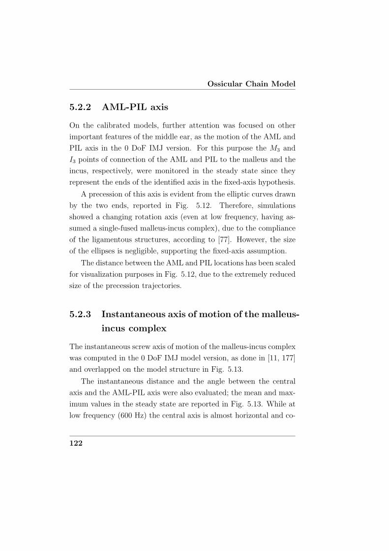
Ossicular Chain Model
5.2.2 AML-PIL axis
On the calibrated models, further attention was focused on other
important features of the middle ear, as the motion of the AML and
PIL axis in the 0 DoF IMJ version. For this purpose the M3 and
I3 points of connection of the AML and PIL to the malleus and the
incus, respectively, were monitored in the steady state since they
represent the ends of the identified axis in the fixed-axis hypothesis.
A precession of this axis is evident from the elliptic curves drawn
by the two ends, reported in Fig. 5.12. Therefore, simulations
showed a changing rotation axis (even at low frequency, having as-
sumed a single-fused malleus-incus complex), due to the compliance
of the ligamentous structures, according to [77]. However, the size
of the ellipses is negligible, supporting the fixed-axis assumption.
The distance between the AML and PIL locations has been scaled
for visualization purposes in Fig. 5.12, due to the extremely reduced
size of the precession trajectories.
5.2.3 Instantaneous axis of motion of the malleus-
incus complex
The instantaneous screw axis of motion of the malleus-incus complex
was computed in the 0 DoF IMJ model version, as done in [11, 177]
and overlapped on the model structure in Fig. 5.13.
The instantaneous distance and the angle between the central
axis and the AML-PIL axis were also evaluated; the mean and max-
imum values in the steady state are reported in Fig. 5.13. While at
low frequency (600 Hz) the central axis is almost horizontal and co-
122
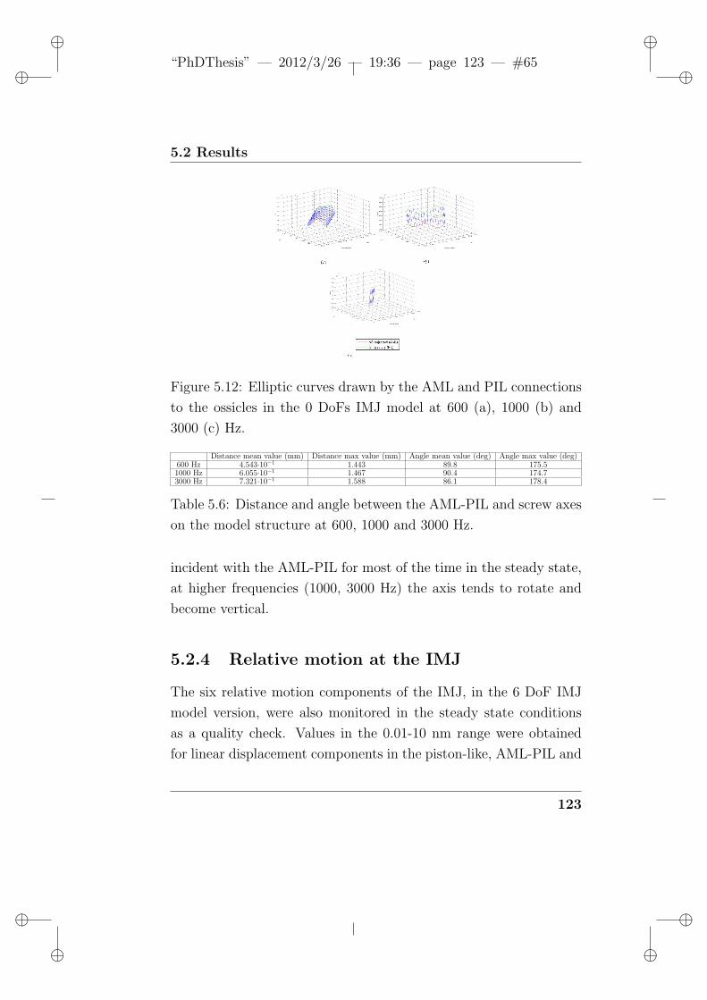
ii
“PhDThesis” — 2012/3/26 — 19:36 — page 123 — #65 ii
ii
ii
5.2 Results
Figure 5.12: Elliptic curves drawn by the AML and PIL connections
to the ossicles in the 0 DoFs IMJ model at 600 (a), 1000 (b) and
3000 (c) Hz.
Distance mean value (mm) Distance max value (mm) Angle mean value (deg) Angle max value (deg)600 Hz 4.543·10−1 1.443 89.8 175.51000 Hz 6.055·10−1 1.467 90.4 174.73000 Hz 7.321·10−1 1.588 86.1 178.4
Table 5.6: Distance and angle between the AML-PIL and screw axes
on the model structure at 600, 1000 and 3000 Hz.
incident with the AML-PIL for most of the time in the steady state,
at higher frequencies (1000, 3000 Hz) the axis tends to rotate and
become vertical.
5.2.4 Relative motion at the IMJ
The six relative motion components of the IMJ, in the 6 DoF IMJ
model version, were also monitored in the steady state conditions
as a quality check. Values in the 0.01-10 nm range were obtained
for linear displacement components in the piston-like, AML-PIL and
123
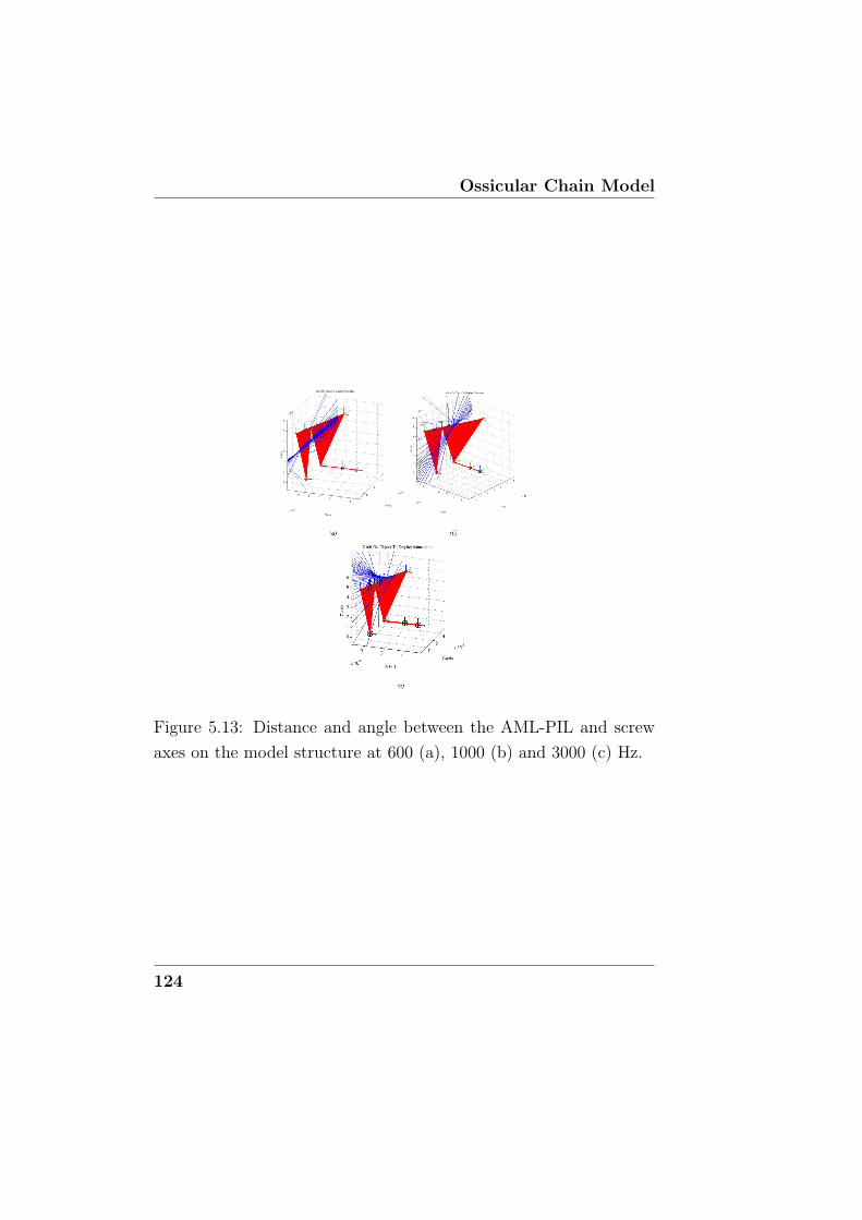
Ossicular Chain Model
Figure 5.13: Distance and angle between the AML-PIL and screw
axes on the model structure at 600 (a), 1000 (b) and 3000 (c) Hz.
124
ii
“PhDThesis” — 2012/3/26 — 19:36 — page 125 — #66 ii
ii
ii
5.3 Discussion
vertical directions.
5.3 Discussion
In this chapter a MB model was proposed, which eases the com-
putational aspect and allows improving the joint behavior as ideal
mechanical joints. The simulation and prediction of the OC behav-
ior was focused on some issues related to the IMJ mobility, came
up from the literature survey. At this purpose two versions of the
model were developed assigning 0 or 6 DoFs to the IMJ.
A calibration procedure was applied to tune uncertain parame-
ters, in particular those whose values were found the most scattered
in the survey. With respect to the literature, where details on the
model calibration are rarely reported, the present study deepens also
that aspect, specifying the objective function, identified parameters
and making a comparison between a local optimization algorithm
and a global one. The first method requires initial guess values,
which can have an influence on the solution; on the other side the
global optimization needs only the definition of boundaries for the
parameters and in this sense could be more reliable. However, no
significant differences were noticed in the results obtained with the
different optimization algorithms.
The proposed MB model succeeded in satisfactorily replicating
both experimental and numerical reference SFP displacements [93],
even with a better response compared to the reference FE model.
To explain this particularity, it is worth noting that the differences
between our model and the reference one, mainly regard the joint
125
Ossicular Chain Model
and cochlear modeling. In [93] the IMJ is modeled as a bone-like
layer between the malleus and the incus (0 DoF), while the TMMJ
and ISJ are modeled as portions of elastic tissues with mechanical
properties taken from [15, 95]. In our model ideal mechanical joints
were used with spring and damper elements characterized by means
of a calibration procedure. Moreover in [93] an uncoiled cochlea was
modeled, while we assumed a mass and damper cochlear load as in
[15].
Our results showed lower amplitude and phase angle RMS errors
for the numerical curve than for the experimental one. The 6 DoF
IMJ version of the model performed better than the 0 DoF one,
showing a lower error. In particular, as highlighted by a separate
calibration on two restricted frequency ranges (< 1 kHz, > 1 kHz),
the main differences between the two model versions arise at high
frequency, the 6 DoF attaining an error around 16% versus a 30%
error of the 0 DoF model. On the other side, at low frequencies
the error is almost the same (24%). These comparative results sug-
gest improvement of joint modeling as a way to enhance FE model
performance.
It is interesting to underline that neglecting the phase angle er-
ror in the objective function gave the lowest error in amplitude (∼8%) maintaining a satisfactory approximation of the phase angle
curve with an average error comparable to the other cases (17.9%
vs. 13.6%). The introduction of an A-weighted objective function
resulted in a higher error, mainly at the boundaries of the frequency
range.
On the calibrated models, further attention was focused on other
important features of the middle ear. The AML-PIL axis displace-
126
ii
“PhDThesis” — 2012/3/26 — 19:36 — page 127 — #67 ii
ii
ii
5.3 Discussion
ment was observed in the 0 DoF IMJ version, both at low and high
frequencies, describing an elliptic precession trajectory, although of
very small amplitude. The instantaneous screw axis of motion was
also computed and the distance and angle between this axis and the
AML-PIL axis were monitored.
Due to its simplicity, physical foundations and good performance,
the proposed MB model may represent a convenient and effective
tool to quickly assess the benefits and risks of middle ear interven-
tions and implants or to estimate the consequences of pathologies In
fact, the main mechanical damages which influence the OC mobil-
ity (e.g. fixation or disruption) can be associated with a variation
of the geometrical and/or the mechanical properties of the struc-
tures, and can be simulated by simply changing model parameters
[178, 102, 116, 66].
As future developments, the introduction of other parts of the
ear in the model will be pursued. A more accurate cochlear load
estimation, as well as a more realistic representation of the complex
connection between the TM and the malleus, certainly could improve
the present model in finding more meaningful parameters, directly
correlated to physical quantities and measurable variables. For this
purpose a hybrid modeling approach, coupling an MB model of the
OC and a FE model of the TM, could help overcoming some concerns
affecting the middle ear simulation [179, 180], as described in the
following chapter.
127

Ossicular Chain Model
128
ii
“PhDThesis” — 2012/3/26 — 19:36 — page 129 — #68 ii
ii
ii
Chapter 6
Hybrid middle ear model
The middle ear models in the literature are typically defined either
in a FE or in a MB environment. As detailed in §4, the FE method
is capable of representing the complex geometry and the material
orthotropy of the TM. On the contrary, a multi-body approach can
be adopted for the OC (§5).
In this section, a complete middle ear model is presented com-
bining the FE model of the TM, described in §4, with the MB model
of the 6 DoF IMJ version of the OC model, described in §5. The
hybrid FE/MB modeling approach was pursued through a feedback
control strategy. Model parameters were estimated (in a first study
[180]) through a calibration procedure with the aim of reproducing
ascertained experimental literature data [93] in terms of umbo (ref-
erence point of connection between the malleus and the TM) and
stapes footplate centre displacements.
The sensitivity of the calibrated model to both TM and OC pa-
rameters was investigated. Material, geometrical and inertial pa-
129
Hybrid middle ear model
rameters were considered, in particular those whose values are most
widespread in the literature.
6.1 Model components
6.1.1 Tympanic membrane finite element model
Th FE model of the human TM as isolated from the middle ear
system, Fig. 6.1 was deduced as detailed by the authors in §4.
Thicknesses and material properties were deduced from [93, 15,
95] which developed a FE model of the middle ear, in order to repli-
cate the characteristics and the numerical/experimental results of
this reference research group. Briefly, the PT and the PF of the TM
are assumed as orthotropic (with a 35 MPa and a 20 MPa values of
the Young’s moduli in the radial and circumferential directions, re-
spectively) and isotropic materials (with a 10 MPa Young’s module),
respectively.
The TA was modeled with shell elements, whose thickness has
a value of 200 m. Differing from [161], a rigid region is defined,
corresponding to the insertion of the manubrium of the malleus into
the TM.
Simulations were carried out in Ansysr 11. A study of conver-
gence, based on the first frequency above 20 kHz, was performed to
set the element size.
130
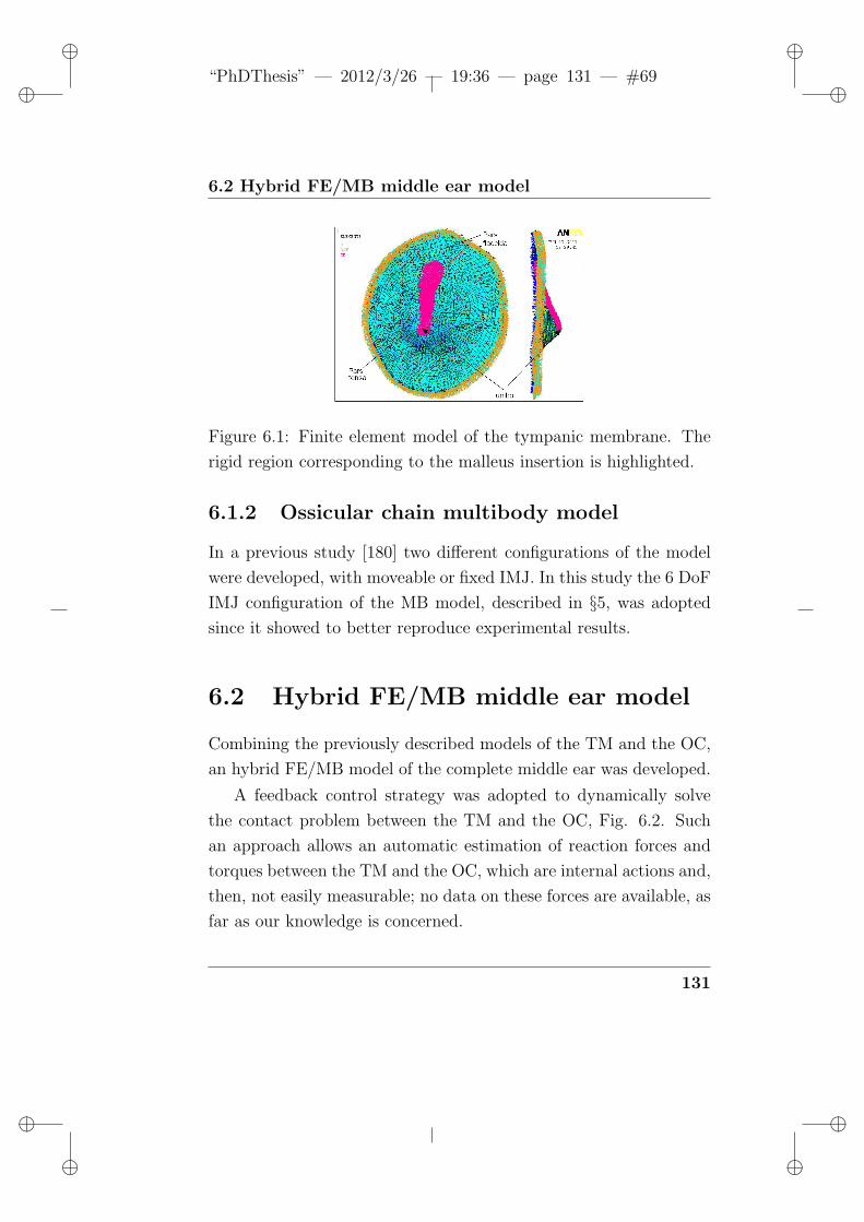
ii
“PhDThesis” — 2012/3/26 — 19:36 — page 131 — #69 ii
ii
ii
6.2 Hybrid FE/MB middle ear model
Figure 6.1: Finite element model of the tympanic membrane. The
rigid region corresponding to the malleus insertion is highlighted.
6.1.2 Ossicular chain multibody model
In a previous study [180] two different configurations of the model
were developed, with moveable or fixed IMJ. In this study the 6 DoF
IMJ configuration of the MB model, described in §5, was adopted
since it showed to better reproduce experimental results.
6.2 Hybrid FE/MB middle ear model
Combining the previously described models of the TM and the OC,
an hybrid FE/MB model of the complete middle ear was developed.
A feedback control strategy was adopted to dynamically solve
the contact problem between the TM and the OC, Fig. 6.2. Such
an approach allows an automatic estimation of reaction forces and
torques between the TM and the OC, which are internal actions and,
then, not easily measurable; no data on these forces are available, as
far as our knowledge is concerned.
131
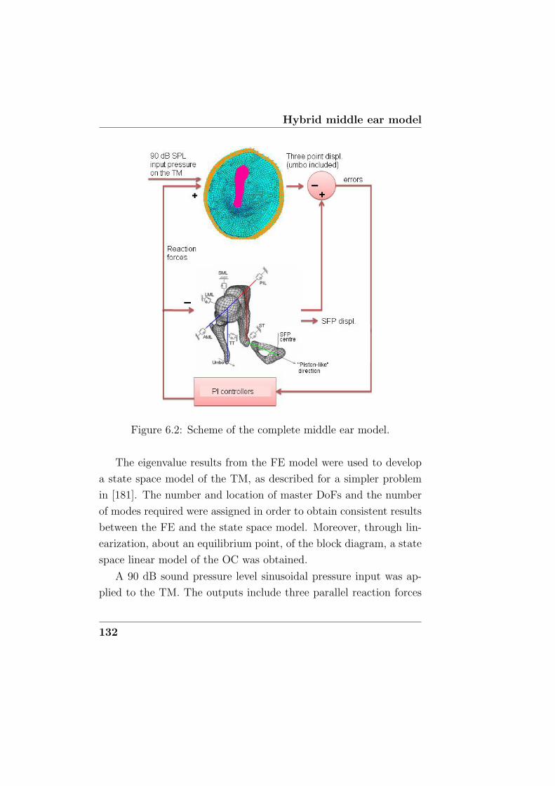
Hybrid middle ear model
Figure 6.2: Scheme of the complete middle ear model.
The eigenvalue results from the FE model were used to develop
a state space model of the TM, as described for a simpler problem
in [181]. The number and location of master DoFs and the number
of modes required were assigned in order to obtain consistent results
between the FE and the state space model. Moreover, through lin-
earization, about an equilibrium point, of the block diagram, a state
space linear model of the OC was obtained.
A 90 dB sound pressure level sinusoidal pressure input was ap-
plied to the TM. The outputs include three parallel reaction forces
132
ii
“PhDThesis” — 2012/3/26 — 19:36 — page 133 — #70 ii
ii
ii
6.2 Hybrid FE/MB middle ear model
between TM and OC on three misaligned points of the rigid region
(umbo included), the umbo and SFP displacement, and the residual
errors at the steady state.
Three proportional-integral controllers were introduced. Three
error functions are provided as inputs to the controllers. Each error
function is computed as the difference between the current displace-
ment value, estimated by the model, and the reference one, deduced
from the literature [93], of each mentioned point. The gain values
were tuned in order to have an error dynamics faster than the system
dynamics.
6.2.1 Parameter identification procedure
The values of umbo and SFP displacement (peak-to-peak amplitude)
assumed as reference signals for the parameter identification proce-
dure were taken from published experimental data [93].
As done for the OC model and described in §5, an optimization
procedure was developed in order to identify unspecified parameters
but also to tune some parameters whose literature values range over
orders of magnitude, as detailed in [180].
6.2.2 Sensitivity analysis
A sensitivity analysis was carried out varying the TM FE model
and the OC MB model parameters, each at a time with respect to
the identified ones. The umbo and SFP displacement curves were
monitored. Concerning the TM model, the selected parameters were:
• the thicknesses of the PT, PF and of the TA;
133
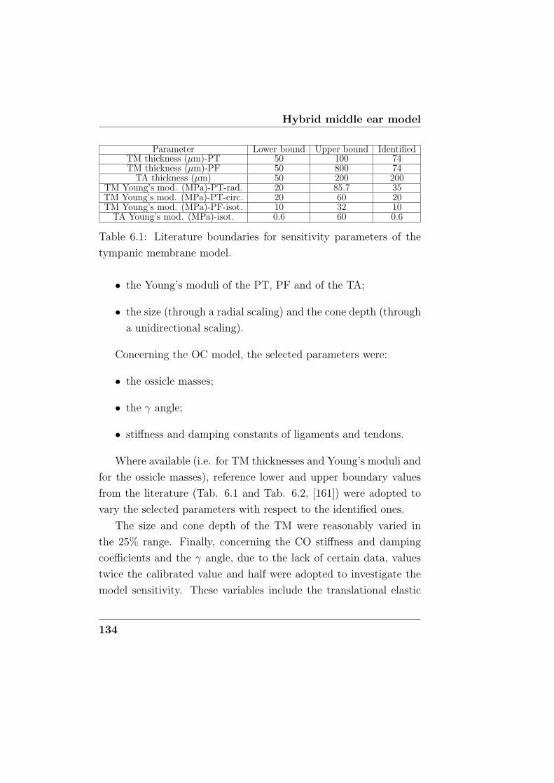
Hybrid middle ear model
Parameter Lower bound Upper bound IdentifiedTM thickness (µm)-PT 50 100 74TM thickness (µm)-PF 50 800 74
TA thickness (µm) 50 200 200TM Young’s mod. (MPa)-PT-rad. 20 85.7 35TM Young’s mod. (MPa)-PT-circ. 20 60 20TM Young’s mod. (MPa)-PF-isot. 10 32 10
TA Young’s mod. (MPa)-isot. 0.6 60 0.6
Table 6.1: Literature boundaries for sensitivity parameters of the
tympanic membrane model.
• the Young’s moduli of the PT, PF and of the TA;
• the size (through a radial scaling) and the cone depth (through
a unidirectional scaling).
Concerning the OC model, the selected parameters were:
• the ossicle masses;
• the γ angle;
• stiffness and damping constants of ligaments and tendons.
Where available (i.e. for TM thicknesses and Young’s moduli and
for the ossicle masses), reference lower and upper boundary values
from the literature (Tab. 6.1 and Tab. 6.2, [161]) were adopted to
vary the selected parameters with respect to the identified ones.
The size and cone depth of the TM were reasonably varied in
the 25% range. Finally, concerning the CO stiffness and damping
coefficients and the γ angle, due to the lack of certain data, values
twice the calibrated value and half were adopted to investigate the
model sensitivity. These variables include the translational elastic
134
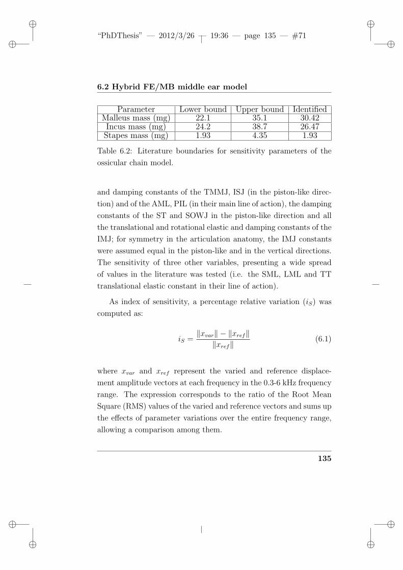
ii
“PhDThesis” — 2012/3/26 — 19:36 — page 135 — #71 ii
ii
ii
6.2 Hybrid FE/MB middle ear model
Parameter Lower bound Upper bound IdentifiedMalleus mass (mg) 22.1 35.1 30.42Incus mass (mg) 24.2 38.7 26.47
Stapes mass (mg) 1.93 4.35 1.93
Table 6.2: Literature boundaries for sensitivity parameters of the
ossicular chain model.
and damping constants of the TMMJ, ISJ (in the piston-like direc-
tion) and of the AML, PIL (in their main line of action), the damping
constants of the ST and SOWJ in the piston-like direction and all
the translational and rotational elastic and damping constants of the
IMJ; for symmetry in the articulation anatomy, the IMJ constants
were assumed equal in the piston-like and in the vertical directions.
The sensitivity of three other variables, presenting a wide spread
of values in the literature was tested (i.e. the SML, LML and TT
translational elastic constant in their line of action).
As index of sensitivity, a percentage relative variation (iS) was
computed as:
iS =‖xvar‖ − ‖xref‖‖xref‖
(6.1)
where xvar and xref represent the varied and reference displace-
ment amplitude vectors at each frequency in the 0.3-6 kHz frequency
range. The expression corresponds to the ratio of the Root Mean
Square (RMS) values of the varied and reference vectors and sums up
the effects of parameter variations over the entire frequency range,
allowing a comparison among them.
135
Hybrid middle ear model
6.3 Results
As results of the calibration procedures, umbo and SFP displacement
amplitudes, fitted on experimental data [93], are shown in Fig. 6.3
and Fig. 6.4 as reference curves. The sensitivity analysis results are
presented in details in the following sections.
6.3.1 Tympanic membrane parameters
TM model sensitivity to size and cone depth features, was evalu-
ated in terms of variations of umbo and SFP displacement curves,
Fig.6.3a-b.
Size is definitely more influential than cone depth and marked
variations appear especially in the high frequency range where an
increase in size produces lower umbo and SFP displacements while
an opposite trend occurs in the low frequency range.
The influence of the TM and TA thickness and Young’s modulus
is evident in Fig. 6.3c-d. A thickness increase produces lower umbo
displacements at all frequencies while for the SFP that is observed
only at high frequencies.
Concerning the Young’s modulus, a noticeable decrease in dis-
placement amplitudes at low frequency arises at high values of the
elastic moduli, especially for the SFP, while at high frequency dis-
placements appear unaffected in both cases.
It is worth noting that the reference values are close to the lower
boundary of the assigned values so that variations on displacements
are negligible.
136
ii
“PhDThesis” — 2012/3/26 — 19:36 — page 137 — #72 ii
ii
ii
6.3 Results
6.3.2 Ossicular chain parameters
The sensitivity of the OC model to ossicles masses and the γ angle,
was evaluated in terms of umbo and SFP displacement curves varia-
tions, Fig.6.4a-b. The influence of the elastic and damping constants
is evident in Fig. 6.4c-d.
Results show a small influence of the assigned mass values on the
curves, while a high influence of the γ angle is evident, mainly in the
SFP curve, with lower displacement amplitudes for greater angles;
for the umbo the influence of γ is limited to the low frequency range.
Considering the elastic and damping constants, a higher influence
on the umbo displacement curve of the former with respect to the
latter appears, while their influence on the SFP curve is comparable.
For the umbo, higher variations mainly arise at low frequencies and
an increase of the elastic constants produces an amplitude decrease.
For the SFP an inversion of such a trend appears at high frequency
while as regards the influence of damping, an increase of it produces,
in general, lower amplitudes. Sensitivity indexes The sensitivity in-
dexes for the TM and OC parameters are reported in Tab. 6.3 and
Tab. 6.4, respectively.
The index signs are consistent with those of the parameter vari-
ations but for TM thickness and OC masses on SFP. Moreover the
indexes appear to depend, in various cases, on the parameter vari-
ation magnitude indicating a non-linear dependence. In particular,
higher sensitivity index values are obtained varying the TM thick-
nesses and increasing the Young’s moduli.
Considering the sensitivity index values for the umbo response,
the OC elastic constants and a decreasing γ angle appear to cause
137
Hybrid middle ear model
Parameter Umbo(%) Stapes(%)Size (lower) -8.54 -8.16Size (upper) 8.52 7.47
Cone depth (lower) 4.78 7.66Cone depth (upper) -4.60 -6.25Thickness (lower) 26.98 37.99Thickness (upper) -21.78 6.30
Young’s modulus (lower) 2.57 5.62Young’s modulus (upper) -51.53 -60.76
Table 6.3: Tympanic membrane parameter sensitivity index.
higher variations. Concerning the SFP response, high values of the
sensitivity indexes arise varying the γ angle and the damping con-
stants.
6.4 Discussion
In the present chapter, a hybrid FE/MB middle ear model was in-
troduced, where a FE model of the TM is connected to a MB scheme
of the OC through a feedback strategy.
The sensitivity of the complete model was evaluated distinguish-
ing the TM and the OC parameters in order to test its robustness to
uncertainties. Geometric (size, cone depth and thickness) and ma-
terial (Young’s modulus) parameters of the TM and annulus were
varied in the FE part of the model. Geometric (γ angle), inertial (os-
sicle masses) and material (elastic and damping constants) param-
eters of the OC and surrounding structures of the tympanic cavity
(joints, ligaments and muscle tendons) were varied in the MB part of
138
ii
“PhDThesis” — 2012/3/26 — 19:36 — page 139 — #73 ii
ii
ii
6.4 Discussion
Parameter Umbo(%) Stapes(%)OC masses (lower) 0-62 0.46OC masses (upper) -1.45 7.11γ angle (lower) 43.31 157.76γ angle (upper) -3.97 -58.86
Elastic const. (lower) 49.87 19.49Elastic const. (upper) -35.26 -19.91
Damping const. (lower) 8.22 36.05Damping const. (upper) -5.22 -32.57
Table 6.4: Ossicular chain parameter sensitivity index.
the model. The effect of parameters variations on umbo and stapes
footplate centre displacement curves was examined with respect to a
reference curve previously calibrated on literature experimental data
[93].
As far as the TM model is concerned, the results show a higher
sensitivity to thickness, and to the increased Young’s moduli. On
the other side for the MB model of the OC, the results show a higher
sensitivity to the γ angle and to the elastic/damping constants in
the umbo/stapes curves.
A patient-specific application involves an unavoidable variation
in parameter values. The availability of accurate ex vivo and in vivo
experimental data could help to limit uncertainties and increase the
model reliability to simulate pathological/post-surgical/post-traumatic
conditions and evaluate ossicular replacement prostheses. However,
some influential parameters (e.g. the damping constants) are still
not easily measurable and their determination will still require the
application of identification techniques.
139
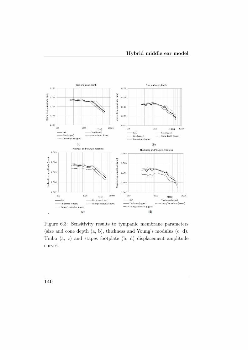
Hybrid middle ear model
Figure 6.3: Sensitivity results to tympanic membrane parameters
(size and cone depth (a, b), thickness and Young’s modulus (c, d).
Umbo (a, c) and stapes footplate (b, d) displacement amplitude
curves.
140
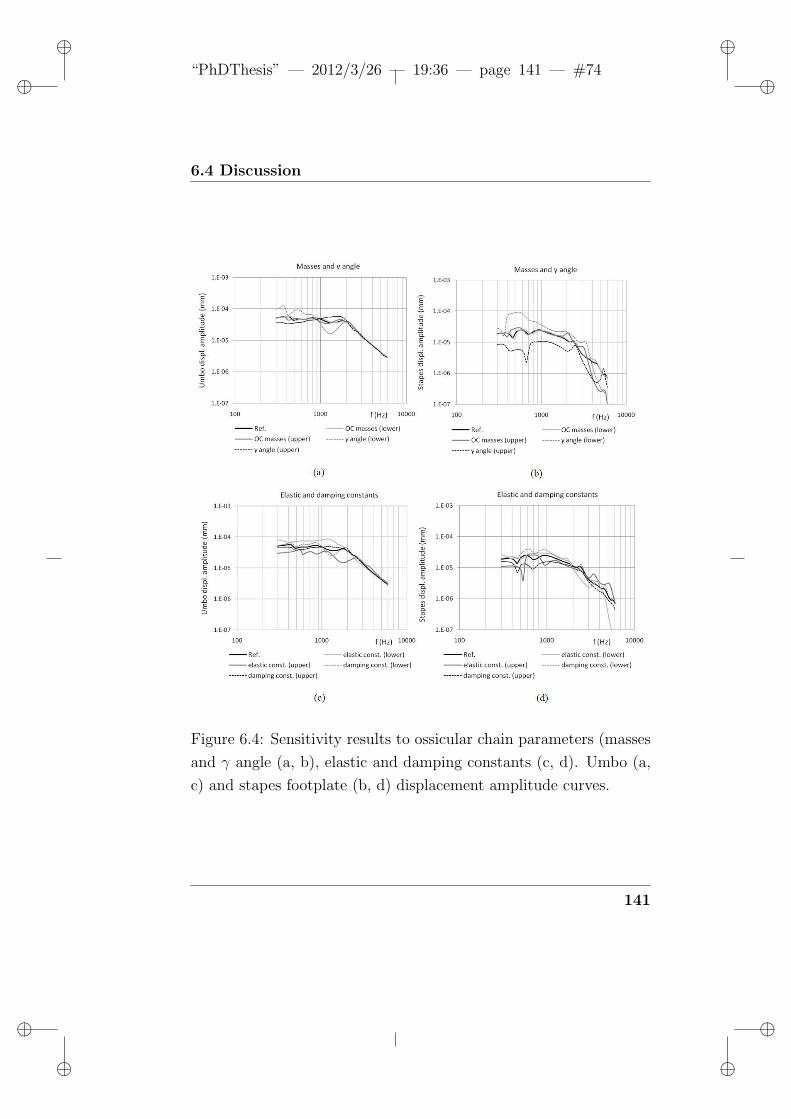
ii
“PhDThesis” — 2012/3/26 — 19:36 — page 141 — #74 ii
ii
ii
6.4 Discussion
Figure 6.4: Sensitivity results to ossicular chain parameters (masses
and γ angle (a, b), elastic and damping constants (c, d). Umbo (a,
c) and stapes footplate (b, d) displacement amplitude curves.
141

Hybrid middle ear model
142
ii
“PhDThesis” — 2012/3/26 — 19:36 — page 143 — #75 ii
ii
ii
Chapter 7
Psychoacoustics
Psychoacoustics, which is a branch of acoustics, deals with the re-
lationships between the physical characteristics of sounds and their
perceptual attributes [5, 182]. It is concerned with the frequency-
dependent sensitivity of the auditory system, the masking processes,
the loudness, pitch and timbre perception of sounds.
The information processing in the auditory system, in terms of
preprocessing in the peripheral system (outer, middle and inner ear)
and neural processing, both including non-linearities, is a central
issue of the psychoacoustic approach. The most important physical
magnitude for psychoacoustics is the time-varying sound pressure, in
the 10−5-102 Pa amplitude range and in the 20 Hz- 20 kHz frequency
range.
Psychoacoustic methodologies were investigated and applied within
the project ”Supporto tecnico per la revisione e l’aggiornamento di
procedure per il calcolo di componenti MAGNA” in collaboration
between the Department of Mechanical, Nuclear and Production En-
143
Psychoacoustics
gineering of the University of Pisa and Magna Closures S.p.A. from
March 2011. The research activity mainly focused on power windows
acoustics for automotive application and included experimental and
theoretical activities, as detailed in §7.3.2 and §7.3.3, respectively.
The main objective of this study was to reproduce and predict the
customers’opinion.
A first work package (RL 1280, April 2011) included the identifi-
cation of suitable theoretical models of noise perception for automo-
tive products, particularly referring to the state of the art on power
window noise characterization, as detailed in §7.3.1. A second work
package (RL 1291, December 2011) included the data processing and
analysis of experimentally acquired signals, as described in §7.3.2 and
§7.3.3. The project is still in progress and the future developments
include a jury test as well as the validation of a computational modal
and acoustic model with the aim to have an instrument to reproduce
and predict the customers’perception, to simulate and design power
windows mounted on car doors.
7.1 Characteristics of sounds and hear-
ing area
Temporal and spectral characteristics of sound are frequently used
in psychoacoustics [182]. The time varying sound pressure (Pa) is
typically referenced. In order to account for such a broad range, the
sound pressure level (SPL, dB) was introduced and defined as [182]:
SPL(dB) = 20 log10
(prmsp0
)(7.1)
144
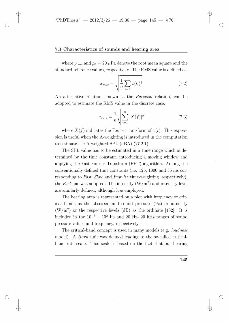
ii
“PhDThesis” — 2012/3/26 — 19:36 — page 145 — #76 ii
ii
ii
7.1 Characteristics of sounds and hearing area
where prms and p0 = 20 µPa denote the root mean square and the
standard reference values, respectively. The RMS value is defined as:
xrms =
√√√√ 1
n
n∑i=1
x(ti)2 (7.2)
An alternative relation, known as the Parseval relation, can be
adopted to estimate the RMS value in the discrete case:
xrms =1
n
√√√√ n∑i=1
|X(f)|2 (7.3)
where X(f) indicates the Fourier transform of x(t). This expres-
sion is useful when the A-weighting is introduced in the computation
to estimate the A-weighted SPL (dBA) (§7.2.1).
The SPL value has to be estimated in a time range which is de-
termined by the time constant, introducing a moving window and
applying the Fast Fourier Transform (FFT) algorithm. Among the
conventionally defined time constants (i.e. 125, 1000 and 35 ms cor-
responding to Fast, Slow and Impulse time-weighting, respectively),
the Fast one was adopted. The intensity (W/m2) and intensity level
are similarly defined, although less employed.
The hearing area is represented on a plot with frequency or crit-
ical bands as the abscissa, and sound pressure (Pa) or intensity
(W/m2) or the respective levels (dB) as the ordinate [182]. It is
included in the 10−5 − 102 Pa and 20 Hz- 20 kHz ranges of sound
pressure values and frequency, respectively.
The critical-band concept is used in many models (e.g. loudness
model). A Bark unit was defined leading to the so-called critical-
band rate scale. This scale is based on the fact that our hearing
145
Psychoacoustics
system analyzes a broad spectrum into parts corresponding to criti-
cal bands.
The concept of critical bands was proposed assuming that the
part of a noise that is effective in masking a test tone is the part of
its spectrum lying near the tone [182]. The width of a critical band
corresponds to a distance along the basilar membrane of about 1.3
mm, representing the ear’s resolving power for simultaneous tones
[182].
At low frequencies, critical bands show a constant width of about
100 Hz, while above 500 Hz critical bands show a bandwidth which
is about 20% of centre frequency [182].
7.2 Psychoacoustic metrics and models
7.2.1 Loudness
Loudness is considered the metric which corresponds most closely to
the sound intensity of a stimulus [182].
Loudness level in phon is defined as the SPL of a 1 kHz tone in
a plane wave and frontal incident that is as loud as the sound in
exam [182]. A 1 kHz, 40 dB SPL tone is assumed as reference for
define 1 sone, the unit of measurement of loudness, corresponding
to 40 phon. The relation between phon and sone units is based on
the fact that an increment of 10 dB (e.g. 20 phon) corresponds to a
doubling in perceived loudness above 40 dB SPL; below 40 dB SPL,
the loudness decreases more quickly [5, 182].
146
ii
“PhDThesis” — 2012/3/26 — 19:36 — page 147 — #77 ii
ii
ii
7.2 Psychoacoustic metrics and models
Equal-loudness contours and A-weighting
The loci of points of equal loudness in the hearing area are called
equal-loudness contours, typically defined for pure tones and for a
frontally incident plane sound field [182].
Some weighting curves were conventionally defined as A, B, C and
D-weighting curves. The A-weighting curve is the most frequently
referenced in the norms and it is obtained reversing the 40 phon
equal-loudness contour.
The equal-loudness contours highlight the loudness dependence
on frequency, while the dependence on bandwidth, frequency content
and duration are not evident. Therefore it is too simple to approx-
imate loudness level of noises or complex tones (or combinations of
both) by the A-weighted SPL [182].
Spectral effects
It is worth considering the uniform exciting noise. The 1 sone value
is reached at 30 dB for uniform exciting noise. The Critical-band
rate may also be used as the abscissa. This scale is more equivalent
to features of our hearing system than frequency.
Band-pass noise of small bandwidths is as loud as the 1-kHz tone
of the same level, up to a certain bandwidth. which corresponds to
the critical bandwidth. Above the critical bandwidth, the loudness
of the band-pass noise increases, clearly indicating the dependence
of loudness on bandwidth [182]. Critical bandwidth plays a very
important role in loudness sensation also for the loudness of two-tone
complexes as a function of the frequency separation of the tones.
Other phenomenons have to be considered in loudness percep-
147
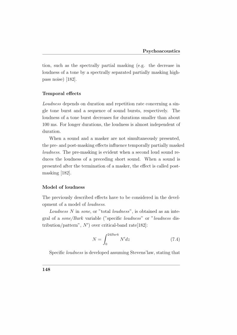
Psychoacoustics
tion, such as the spectrally partial masking (e.g. the decrease in
loudness of a tone by a spectrally separated partially masking high-
pass noise) [182].
Temporal effects
Loudness depends on duration and repetition rate concerning a sin-
gle tone burst and a sequence of sound bursts, respectively. The
loudness of a tone burst decreases for durations smaller than about
100 ms. For longer durations, the loudness is almost independent of
duration.
When a sound and a masker are not simultaneously presented,
the pre- and post-masking effects influence temporally partially masked
loudness. The pre-masking is evident when a second loud sound re-
duces the loudness of a preceding short sound. When a sound is
presented after the termination of a masker, the effect is called post-
masking [182].
Model of loudness
The previously described effects have to be considered in the devel-
opment of a model of loudness.
Loudness N in sone, or ”total loudness”, is obtained as an inte-
gral of a sone/Bark variable (”specific loudness” or ”loudness dis-
tribution/pattern”, N ′) over critical-band rate[182]:
N =
∫ 24Bark
0
N ′dz (7.4)
Specific loudness is developed assuming Stevens’law, stating that
148
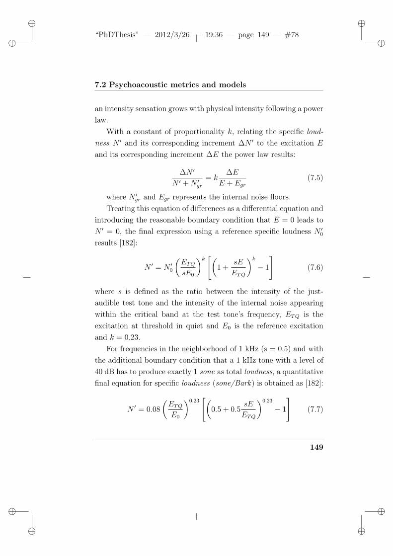
ii
“PhDThesis” — 2012/3/26 — 19:36 — page 149 — #78 ii
ii
ii
7.2 Psychoacoustic metrics and models
an intensity sensation grows with physical intensity following a power
law.
With a constant of proportionality k, relating the specific loud-
ness N ′ and its corresponding increment ∆N ′ to the excitation E
and its corresponding increment ∆E the power law results:
∆N ′
N ′ +N ′gr= k
∆E
E + Egr(7.5)
where N ′gr and Egr represents the internal noise floors.
Treating this equation of differences as a differential equation and
introducing the reasonable boundary condition that E = 0 leads to
N ′ = 0, the final expression using a reference specific loudness N ′0results [182]:
N ′ = N ′0
(ETQsE0
)k [(1 +
sE
ETQ
)k− 1
](7.6)
where s is defined as the ratio between the intensity of the just-
audible test tone and the intensity of the internal noise appearing
within the critical band at the test tone’s frequency, ETQ is the
excitation at threshold in quiet and E0 is the reference excitation
and k = 0.23.
For frequencies in the neighborhood of 1 kHz (s = 0.5) and with
the additional boundary condition that a 1 kHz tone with a level of
40 dB has to produce exactly 1 sone as total loudness, a quantitative
final equation for specific loudness (sone/Bark) is obtained as [182]:
N ′ = 0.08
(ETQE0
)0.23[(
0.5 + 0.5sE
ETQ
)0.23
− 1
](7.7)
149
Psychoacoustics
Loudness calculating procedure
A procedure to calculate specific and total loudness for steady-state
sounds was developed to make use of third-octave band levels and
the implementation was published in DIN 45 631 [182]. A graphical
loudness calculation procedure, part of the ISO 532 B international
standard is described in [182], starting from a chart of the third
octave band levels.
Approximating the human ear’s frequency selectivity through
third-octave band filters instead of critical-band filters involves that
the differences in bandwidth are not 1 Bark and a k = 0.25 value to
account for additional specific loudness towards lower frequencies.
Such an approximation is acceptable above 300 Hz since for lower
frequencies, third octave band are too small with respect to critical
bands. Therefore, the critical-band level has to be approximated
by adding up the sound intensities falling in the given third-octave
bands. For precise measurements, especially in cases where the com-
ponents at very low frequencies are dominant, the procedure can gain
accuracy introducing a tabulated weighting of the frequency compo-
nents below 250 Hz corresponding to the equal loudness contours
[182].
In the present work the specific and total loudness were computed
according to DIN 45631/ISO 532B norm [182] through the available
code1
For time-varying sounds, however, in addition the nonlinear tem-
poral processing of loudness in the human hearing system has to be
simulated in loudness meters. Loudness meters calculate the loud-
1http://www.acoustics.salford.ac.uk/res/cox/sound quality/index.php?content=MATLABcodes
150
ii
“PhDThesis” — 2012/3/26 — 19:36 — page 151 — #79 ii
ii
ii
7.2 Psychoacoustic metrics and models
ness corresponding to ISO 532B almost instantaneously (i.e. using
the same temporal characteristics as our hearing system). In order
to simulate the characteristics of our hearing system, critical-band
analysis has to be done every 2 ms. This means that a filter bank
has to be installed that simulates the frequency selectivity of our
inner ear.
A loudness meter can be made by a filter bank of third-octave-
band filters, accounting also for temporal effects with respect to the
graphical procedure accounting only for the spectral effects. The
sound pressure time function is processed by the filter bank, a recti-
fier and a lowpass with 2 ms time constant producing the temporal
envelope of the outputs [182].
The above mentioned generalization of loudness model, known as
time-varying loudness, was introduced by [183] to account for tempo-
ral effects, according to DIN45631. The algorithm measures the third
octave spectrum using exponential averaging with a 2 ms time con-
stant, combines the fractional-octave bands into critical bands, and
applies temporal and spectral masking, returning the specific loud-
ness versus critical band rate and the integral of the specific loudness,
applying temporal post-masking filters to measure the time-varying
loudness (LabView 2010 Help, National Instruments).
In addition to loudness pattern and time function, statistical
loudness distributions can be estimated, such as the percentile loud-
ness Ni (e.g. loudness value reached or exceeded in i% of the mea-
surement time). Mainly the N90 and N5 values are referred in the
literature [184].
In the power window application described in [185], peak values of
time-varying loudness of a closing phase (i.e. stationary phase with
151
Psychoacoustics
initial and final transients) below to 30 sone, included in the 30-35
sone range or above 35 sone are associated to absence of negative
impact, marginal and significant negative effects on perceived overall
quality and annoyance, respectively.
7.2.2 Sharpness
The sensation of sharpness belongs to the timbre perception, but
it is often considered separately [182]. The spectral envelope and
the centre frequency of narrow-band sounds, rather than the fine
structure, of a sound mainly influences the sensation of sharpness.
A narrow-band noise one critical-band wide at a centre frequency
of 1 kHz having a level of 60 dB is conventionally assumed as refer-
ence sound producing 1 acum (i.e. the sharpness unit of measure-
ment).
For narrow-band noises, sharpness increases with increasing cen-
tre frequency. For centre frequencies below 3 kHz, sharpness in-
creases almost in proportion to critical-band rate. Above 3 kHz
sharpness increases faster than the critical-band rate. This effect
seems to be the reason that very high-frequency sounds produce a
sensation that is dominated by their sharpness. From 200 Hz to 10
kHz, sharpness increases by a factor of 50.
The dependence of sharpness on bandwidth, as long as smaller
than the critical band, can be ignored. However, sharpness is highly
dependent on bandwidth as it is evident observing the sharpness of
band-pass noise as a function of lower and upper cut-off frequency
with an 10 kHz upper and a 0.2 kHz lower cut-off values, respectively
[182].
152
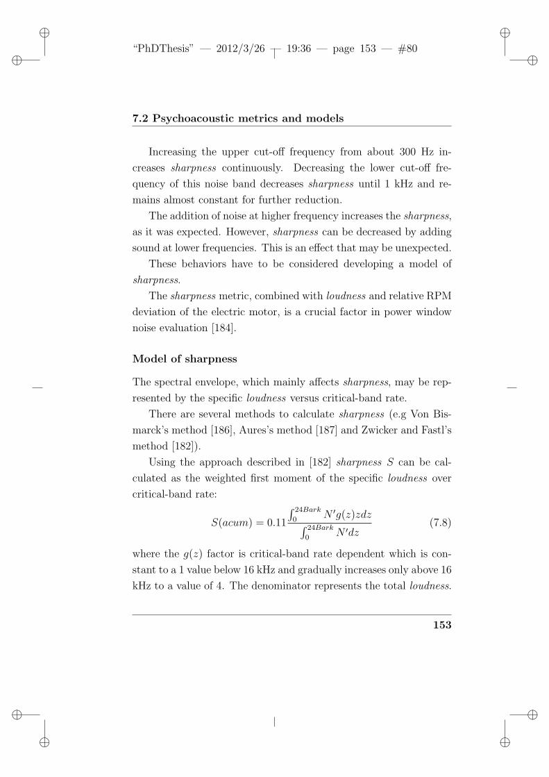
ii
“PhDThesis” — 2012/3/26 — 19:36 — page 153 — #80 ii
ii
ii
7.2 Psychoacoustic metrics and models
Increasing the upper cut-off frequency from about 300 Hz in-
creases sharpness continuously. Decreasing the lower cut-off fre-
quency of this noise band decreases sharpness until 1 kHz and re-
mains almost constant for further reduction.
The addition of noise at higher frequency increases the sharpness,
as it was expected. However, sharpness can be decreased by adding
sound at lower frequencies. This is an effect that may be unexpected.
These behaviors have to be considered developing a model of
sharpness.
The sharpness metric, combined with loudness and relative RPM
deviation of the electric motor, is a crucial factor in power window
noise evaluation [184].
Model of sharpness
The spectral envelope, which mainly affects sharpness, may be rep-
resented by the specific loudness versus critical-band rate.
There are several methods to calculate sharpness (e.g Von Bis-
marck’s method [186], Aures’s method [187] and Zwicker and Fastl’s
method [182]).
Using the approach described in [182] sharpness S can be cal-
culated as the weighted first moment of the specific loudness over
critical-band rate:
S(acum) = 0.11
∫ 24Bark
0N ′g(z)zdz∫ 24Bark
0N ′dz
(7.8)
where the g(z) factor is critical-band rate dependent which is con-
stant to a 1 value below 16 kHz and gradually increases only above 16
kHz to a value of 4. The denominator represents the total loudness.
153
Psychoacoustics
In the present study, specific and total sharpness were computed
as in [182].
7.2.3 Fluctuation strength and roughness
Two different kinds of hearing sensations are produced by modu-
lated sounds: for a modulation frequency below 20 Hz and above
20 Hz, the sensations of fluctuation strength and roughness occur,
respectively, with a smooth transition [182].
A unit of measurement (vacil) of fluctuation strength is defined
for a 60 dB, 1-kHz tone 100% amplitude-modulated at 4Hz. The
unit of measurement of roughness is the asper, defined for a 60 dB
1 kHz tone which is 100% modulated in amplitude with a 70 Hz
modulation frequency.
The fluctuation strength shows a band-pass behavior as a func-
tion of modulation frequency with a maximum at 4 Hz, which cor-
responds to the speaking rate indicating the tuning of the hearing
system during the evolution.
Fluctuation strength depends on SPL, modulation depth or factor
and, in details, :
• increases at increasing SPL;
• is zero until a modulation depth of about 3 dB
• increases approximately linearly with the logarithm of modu-
lation depth, reaching a maximum at 30 dB.
A little and a high dependence of fluctuation strength produced
by amplitude- and frequency-modulated pure tones on centre fre-
quency was shown in [182], respectively.
154
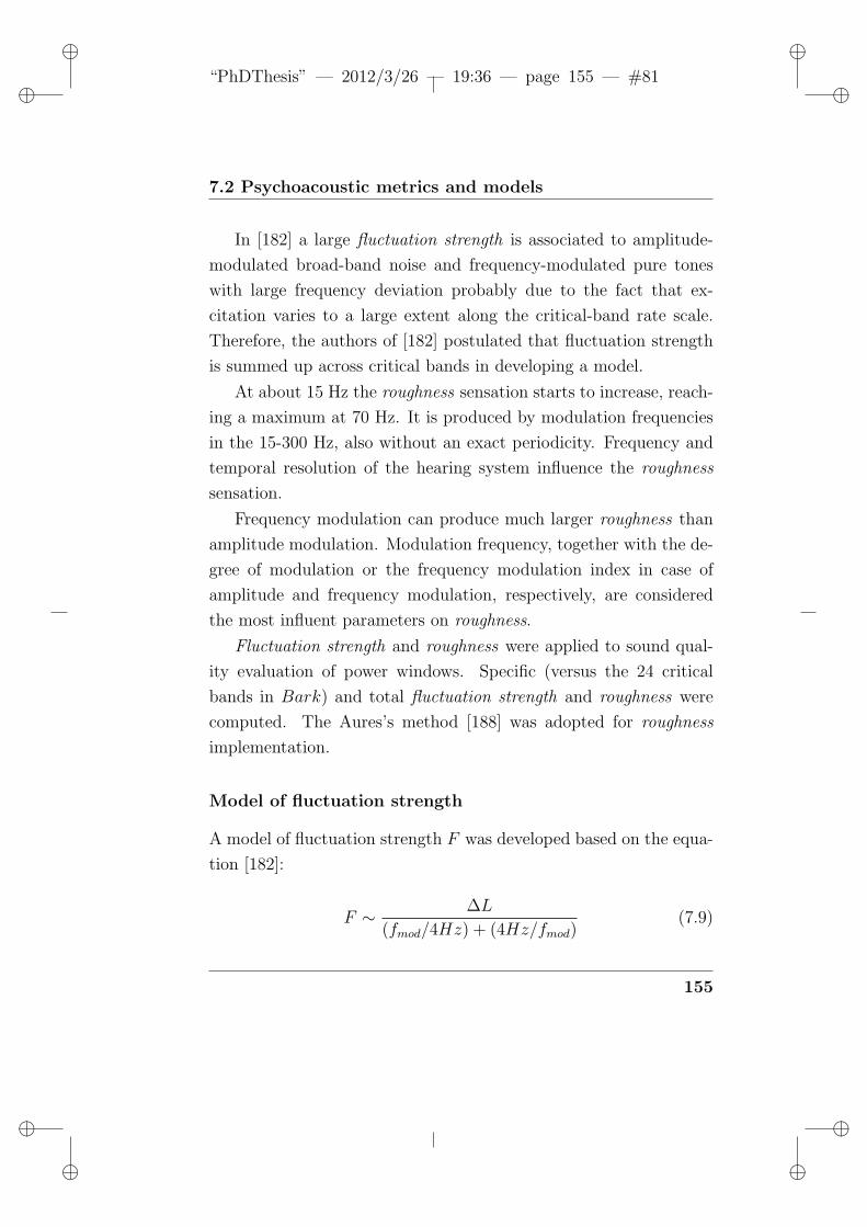
ii
“PhDThesis” — 2012/3/26 — 19:36 — page 155 — #81 ii
ii
ii
7.2 Psychoacoustic metrics and models
In [182] a large fluctuation strength is associated to amplitude-
modulated broad-band noise and frequency-modulated pure tones
with large frequency deviation probably due to the fact that ex-
citation varies to a large extent along the critical-band rate scale.
Therefore, the authors of [182] postulated that fluctuation strength
is summed up across critical bands in developing a model.
At about 15 Hz the roughness sensation starts to increase, reach-
ing a maximum at 70 Hz. It is produced by modulation frequencies
in the 15-300 Hz, also without an exact periodicity. Frequency and
temporal resolution of the hearing system influence the roughness
sensation.
Frequency modulation can produce much larger roughness than
amplitude modulation. Modulation frequency, together with the de-
gree of modulation or the frequency modulation index in case of
amplitude and frequency modulation, respectively, are considered
the most influent parameters on roughness.
Fluctuation strength and roughness were applied to sound qual-
ity evaluation of power windows. Specific (versus the 24 critical
bands in Bark) and total fluctuation strength and roughness were
computed. The Aures’s method [188] was adopted for roughness
implementation.
Model of fluctuation strength
A model of fluctuation strength F was developed based on the equa-
tion [182]:
F ∼ ∆L
(fmod/4Hz) + (4Hz/fmod)(7.9)
155
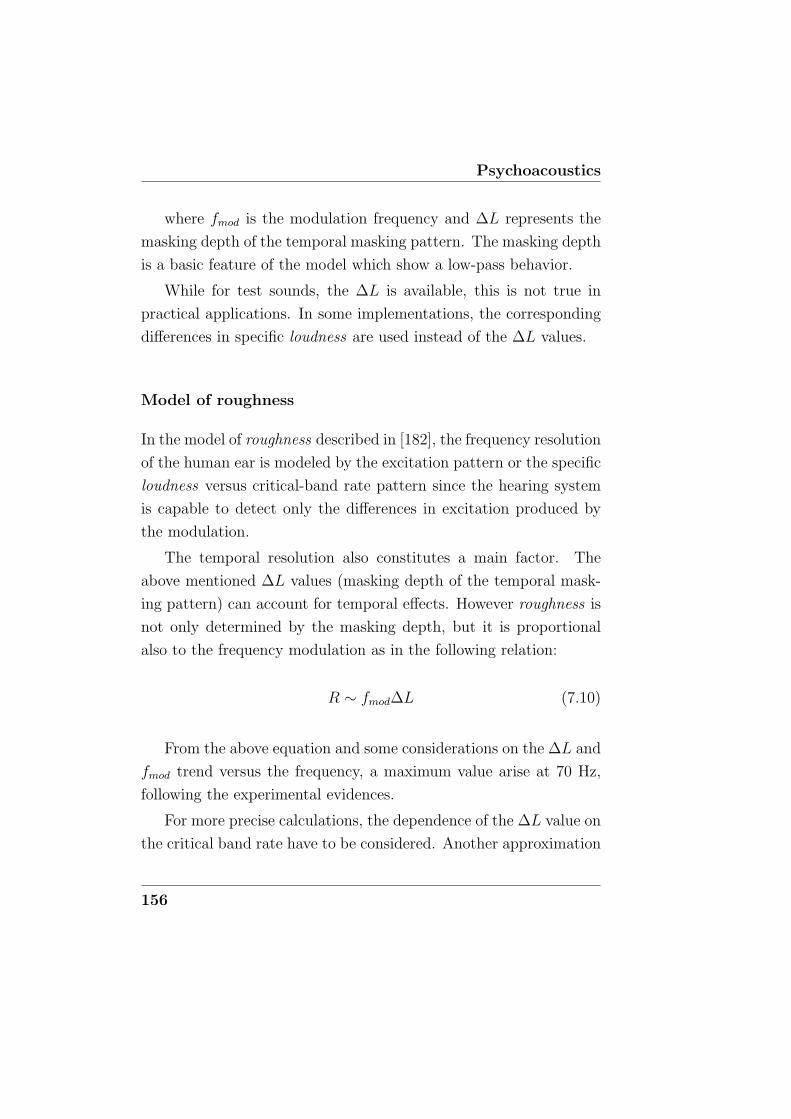
Psychoacoustics
where fmod is the modulation frequency and ∆L represents the
masking depth of the temporal masking pattern. The masking depth
is a basic feature of the model which show a low-pass behavior.
While for test sounds, the ∆L is available, this is not true in
practical applications. In some implementations, the corresponding
differences in specific loudness are used instead of the ∆L values.
Model of roughness
In the model of roughness described in [182], the frequency resolution
of the human ear is modeled by the excitation pattern or the specific
loudness versus critical-band rate pattern since the hearing system
is capable to detect only the differences in excitation produced by
the modulation.
The temporal resolution also constitutes a main factor. The
above mentioned ∆L values (masking depth of the temporal mask-
ing pattern) can account for temporal effects. However roughness is
not only determined by the masking depth, but it is proportional
also to the frequency modulation as in the following relation:
R ∼ fmod∆L (7.10)
From the above equation and some considerations on the ∆L and
fmod trend versus the frequency, a maximum value arise at 70 Hz,
following the experimental evidences.
For more precise calculations, the dependence of the ∆L value on
the critical band rate have to be considered. Another approximation
156
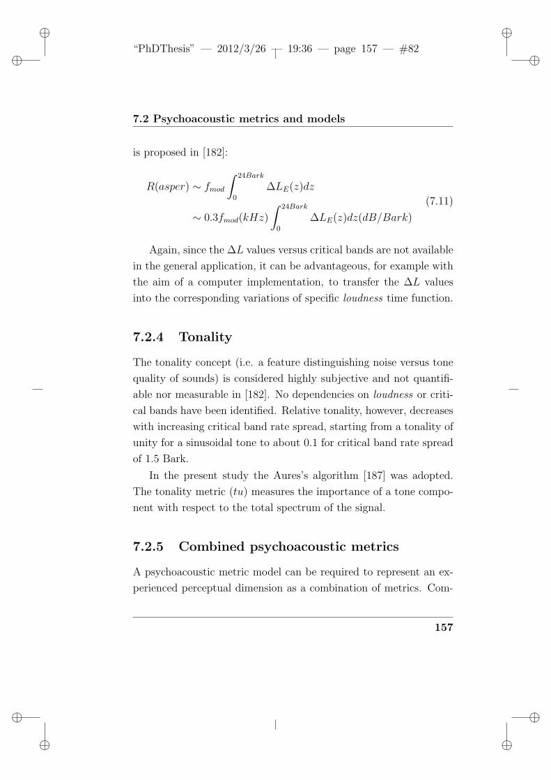
ii
“PhDThesis” — 2012/3/26 — 19:36 — page 157 — #82 ii
ii
ii
7.2 Psychoacoustic metrics and models
is proposed in [182]:
R(asper) ∼ fmod
∫ 24Bark
0
∆LE(z)dz
∼ 0.3fmod(kHz)
∫ 24Bark
0
∆LE(z)dz(dB/Bark)
(7.11)
Again, since the ∆L values versus critical bands are not available
in the general application, it can be advantageous, for example with
the aim of a computer implementation, to transfer the ∆L values
into the corresponding variations of specific loudness time function.
7.2.4 Tonality
The tonality concept (i.e. a feature distinguishing noise versus tone
quality of sounds) is considered highly subjective and not quantifi-
able nor measurable in [182]. No dependencies on loudness or criti-
cal bands have been identified. Relative tonality, however, decreases
with increasing critical band rate spread, starting from a tonality of
unity for a sinusoidal tone to about 0.1 for critical band rate spread
of 1.5 Bark.
In the present study the Aures’s algorithm [187] was adopted.
The tonality metric (tu) measures the importance of a tone compo-
nent with respect to the total spectrum of the signal.
7.2.5 Combined psychoacoustic metrics
A psychoacoustic metric model can be required to represent an ex-
perienced perceptual dimension as a combination of metrics. Com-
157
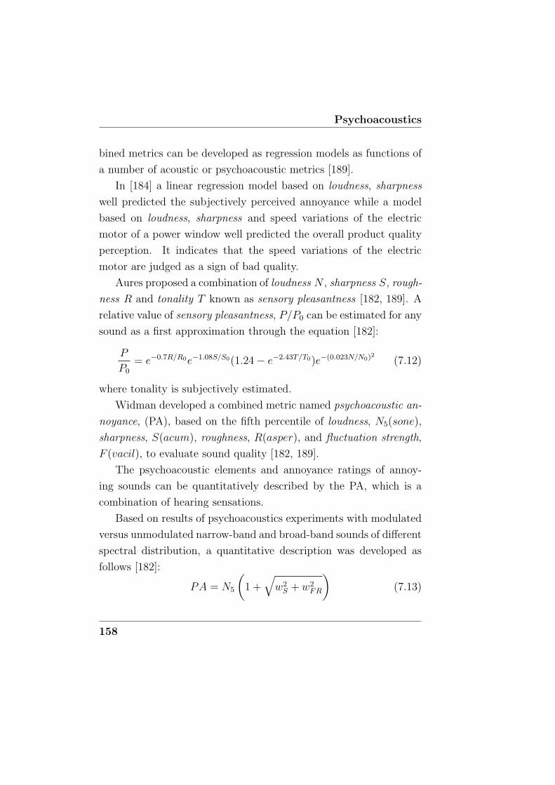
Psychoacoustics
bined metrics can be developed as regression models as functions of
a number of acoustic or psychoacoustic metrics [189].
In [184] a linear regression model based on loudness, sharpness
well predicted the subjectively perceived annoyance while a model
based on loudness, sharpness and speed variations of the electric
motor of a power window well predicted the overall product quality
perception. It indicates that the speed variations of the electric
motor are judged as a sign of bad quality.
Aures proposed a combination of loudness N , sharpness S, rough-
ness R and tonality T known as sensory pleasantness [182, 189]. A
relative value of sensory pleasantness, P/P0 can be estimated for any
sound as a first approximation through the equation [182]:
P
P0
= e−0.7R/R0e−1.08S/S0(1.24− e−2.43T/T0)e−(0.023N/N0)2 (7.12)
where tonality is subjectively estimated.
Widman developed a combined metric named psychoacoustic an-
noyance, (PA), based on the fifth percentile of loudness, N5(sone),
sharpness, S(acum), roughness, R(asper), and fluctuation strength,
F (vacil), to evaluate sound quality [182, 189].
The psychoacoustic elements and annoyance ratings of annoy-
ing sounds can be quantitatively described by the PA, which is a
combination of hearing sensations.
Based on results of psychoacoustics experiments with modulated
versus unmodulated narrow-band and broad-band sounds of different
spectral distribution, a quantitative description was developed as
follows [182]:
PA = N5
(1 +
√w2S + w2
FR
)(7.13)
158
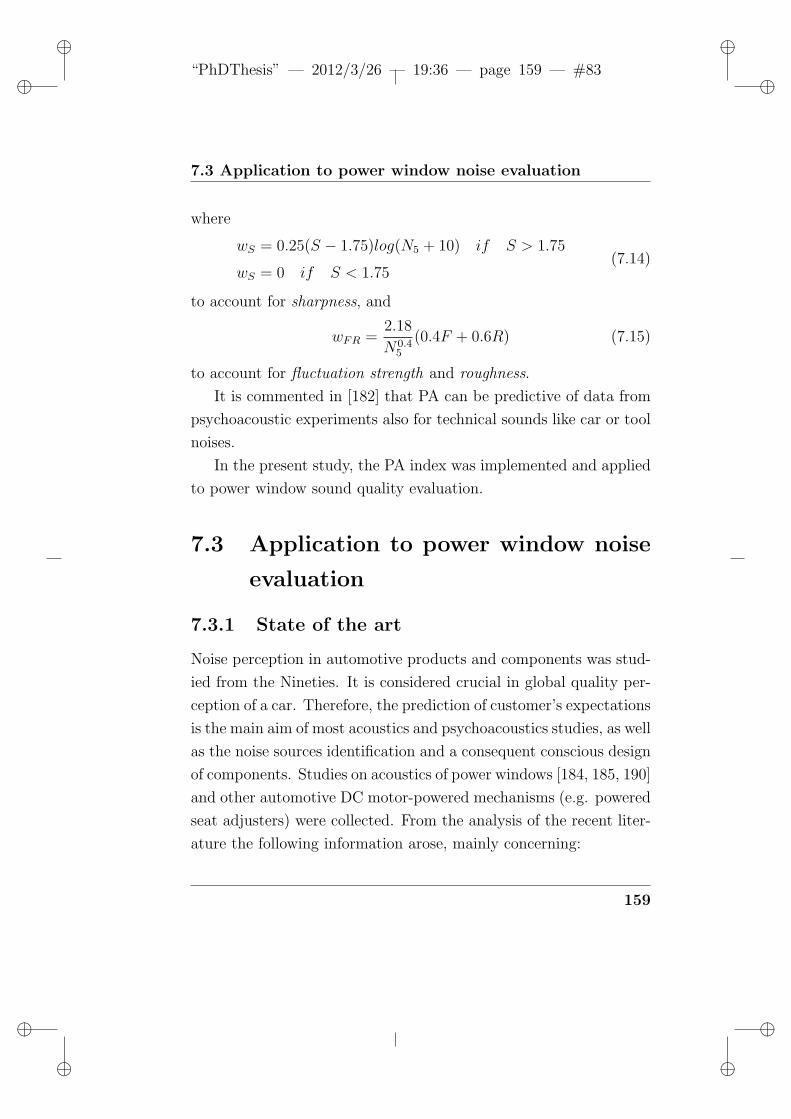
ii
“PhDThesis” — 2012/3/26 — 19:36 — page 159 — #83 ii
ii
ii
7.3 Application to power window noise evaluation
where
wS = 0.25(S − 1.75)log(N5 + 10) if S > 1.75
wS = 0 if S < 1.75(7.14)
to account for sharpness, and
wFR =2.18
N0.45
(0.4F + 0.6R) (7.15)
to account for fluctuation strength and roughness.
It is commented in [182] that PA can be predictive of data from
psychoacoustic experiments also for technical sounds like car or tool
noises.
In the present study, the PA index was implemented and applied
to power window sound quality evaluation.
7.3 Application to power window noise
evaluation
7.3.1 State of the art
Noise perception in automotive products and components was stud-
ied from the Nineties. It is considered crucial in global quality per-
ception of a car. Therefore, the prediction of customer’s expectations
is the main aim of most acoustics and psychoacoustics studies, as well
as the noise sources identification and a consequent conscious design
of components. Studies on acoustics of power windows [184, 185, 190]
and other automotive DC motor-powered mechanisms (e.g. powered
seat adjusters) were collected. From the analysis of the recent liter-
ature the following information arose, mainly concerning:
159
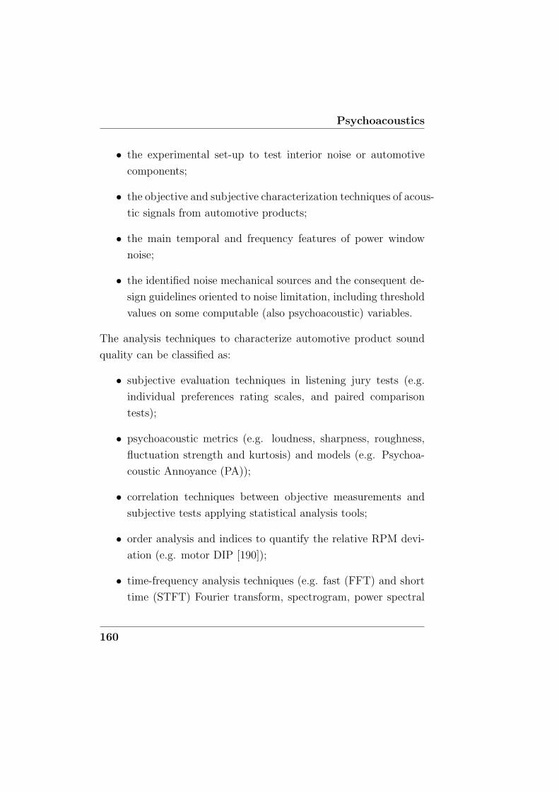
Psychoacoustics
• the experimental set-up to test interior noise or automotive
components;
• the objective and subjective characterization techniques of acous-
tic signals from automotive products;
• the main temporal and frequency features of power window
noise;
• the identified noise mechanical sources and the consequent de-
sign guidelines oriented to noise limitation, including threshold
values on some computable (also psychoacoustic) variables.
The analysis techniques to characterize automotive product sound
quality can be classified as:
• subjective evaluation techniques in listening jury tests (e.g.
individual preferences rating scales, and paired comparison
tests);
• psychoacoustic metrics (e.g. loudness, sharpness, roughness,
fluctuation strength and kurtosis) and models (e.g. Psychoa-
coustic Annoyance (PA));
• correlation techniques between objective measurements and
subjective tests applying statistical analysis tools;
• order analysis and indices to quantify the relative RPM devi-
ation (e.g. motor DIP [190]);
• time-frequency analysis techniques (e.g. fast (FFT) and short
time (STFT) Fourier transform, spectrogram, power spectral
160
ii
“PhDThesis” — 2012/3/26 — 19:36 — page 161 — #84 ii
ii
ii
7.3 Application to power window noise evaluation
density (PSD), third octave band spectrum, cepstrum, Wigner-
Ville distribution and ambiguity function, wavelet transforms);
• artificial neural networks and fuzzy logic, also combined with
wavelet analysis;
• Computer Aided Engineering (CAE) models and, in particular,
FE method, dynamic simulation of elastic bodies and lumped-
parameter models.
7.3.2 Materials and experimental activity
The experimental activity was conducted in three sessions between
April and September 2011 at MAGNA Closures S.p.A in Guasticce
(Collesalvetti, LI) and at the Scalbatraio laboratory in San Piero a
Grado (PI). The instrumentation included a microphone, some ac-
celerometers, a Hall rolling velocity transducer on the electric motor,
an instrumented hammer with a steel tip. Two kinds of tests were
run:
• closing (travelling-up)-opening (travelling-down) event sequences
of the power window rail to evaluate the component noise,
varying the test conditions in terms of input voltage, kind of
DC motor, with or without silent blocks;
• impact tests (”Multiple-reference Impact Test”) with an in-
strumented hammer, to characterize the component dynamic
behavior and to validate a computational model;
with the decoupled component (both in the free-free, or grounded-
grounded test boundary conditions) or fixed to a car door.
161
Psychoacoustics
Additional tests in a semi-anechoic chamber were run at EuroA-
coustics in Avigliana (TO) on November 2011. During this session,
39 decoupled DC motors for power windows were tested in a free-
free condition while 12 power window rails were fixed on a rigid
fixture and tested in different configurations of input voltage and
load, according to technical specifications. Data from microphone
and accelerometers recorded in these acquisitions will be available
for processing in the near future and are not included in the follow-
ing data processing presentation.
7.3.3 Methods and models
Data processing consisted of analysis techniques partially deduced
from the state of the art review. Some general analysis instruments
were applied to the microphone and accelerometer signals to evaluate
sound quality:
• the Sound Pressure Level (SPL) vs. time with ”Fast” time
exponential averaging, with reference value p0 = 20 µPa. An
analogous expression was employed for accelerometer signals
with a reference value a0 = 10−6 m/s2. The SPL was expressed
in dBA applying the A-weighting to account for the different
sensitivity of the human ear in the frequency range. Tempo-
ral characteristics were distinguished into time segments (e.g.
transient initial and stopping events and stationary travelling
phase) by means of a semi-automatic identification based on
the SPL (dBA) function.
• auto- and cross-correlation to evaluate the repeatability of ex-
162
ii
“PhDThesis” — 2012/3/26 — 19:36 — page 163 — #85 ii
ii
ii
7.3 Application to power window noise evaluation
perimental set-up;
• Signal to Noise Ratio (SNR), evaluated on the raw sound pres-
sure time function or on the SPL (dBA), to estimate the ground
noise;
• signal conditioning and filtering techniques, investigated to
limit the measuring noise, to avoid aliasing problems in deci-
mation procedures, to segregate the DC motor sound (¡ 1500
Hz) and most of the window seal scratching (¿ 1500 Hz) [184];
• time-frequency analyses and, in details: FFT of stationary sig-
nals; spectrogram, computed by means of STFT; PSD func-
tion; the third octave band spectrum (dB or dBA).
The following methodologies were applied to the microphone sig-
nal, focusing on the travelling-up segment:
• parameters from customer’s specifications and data sheets in
the time and frequency domains;
• kurtosis function to quantify the squeak phenomenon;
• psychoacoustic metrics and models [182] and, in details: spe-
cific and total loudness (DIN 45631, ISO 532B) for stationary
signals, time-varying loudness and loudness percentiles; total
and specific sharpness, roughness and fluctuation strength; PA
model, a combination of loudness percentile, sharpness, fluc-
tuation strength and roughness metrics.
Scalar parameters were computed to characterize the DC motor
velocity in the closing phases, monitored by a Hall transducer, since
163
Psychoacoustics
motor velocity variations appear to have a high influence on radiated
noise:
• the percentual decrement (”motor DIP”, [190] with respect to
the mean value (RPM) of rotational velocity of the DC motor
and translational velocity of the glass;
• the Relative RPM Deviation (RRD), ”steadiness” metrics [184].
Concerning the impact hammer tests, the accelerometer signals
and hammer load cell were processed applying the following method-
ologies:
• Frequency Response Function (FRF) estimation and partial
completion of the FRF matrix;
• quality checks: reciprocity check (based on the FRF matrix
symmetry) to evaluate the linearity and the quality of the
measurement system; force auto-spectrum, to identify the fre-
quency range of excitation and response; coherence function, to
estimate the degree of linear relation between the input/ouput
signals.
• modal parameter extraction techniques (e.g. Peak Picking
method, ARX/ARMAX models, Least Square Complex Ex-
ponential Method).
7.3.4 Results and discussion
The experimental and theoretical analyses allowed to define and tune
a procedure to investigate the sound quality of power windows. Some
164
ii
“PhDThesis” — 2012/3/26 — 19:36 — page 165 — #86 ii
ii
ii
7.3 Application to power window noise evaluation
methodologies and parameters were introduced and compared with
threshold values from the literature and reference specifications from
data-sheets. From the analysis of the closing-opening sequence sig-
nal, the following conclusions can be drawn:
• the SPL (dBA) time function is highly related to the supply
voltage, to the DC motor type and to the presence of silent
blocks, in terms of temporal phases duration, maximum, mean
and minimum values in the travelling-up phases;
• loudness, a loudness percentile and the integral of the exceed-
ing area of the third octave band spectrum out of a reference
specification mask showed lower values for the V5 motor and
with silent-blocks;
• psychoacoustic metrics and models, such as the PA and the
maximum value of the time-varying loudness were able to dis-
tinguish between test arrangements, although they result con-
troversially related in different sessions;
• the scalar motor DIP and RRD were sensitive to the load con-
ditions of the electric motor. The RPM variation time function
results strictly related to the SPL (dBA) time function of the
microphone signal in all tracks, indicating an high influence on
noise generation;
• in addition to the introduced scalar indices, the analysis of the
spectra of the microphone and accelerometer signals completes
the quantitative and objective description of different experi-
mental configurations.
165
Psychoacoustics
From the analysis of the closing phases, significant differences
arise between tests conducted with the component in different ar-
rangements (decoupled in the free-free or grounded-grounded bound-
ary conditions or mounted on a car door) in terms of duration differ-
ence between travelling-up and travelling-down phases; these differ-
ences can be dependent on the fact that a constant weight does not
exactly reproduce the variable resistance of the seals on the glass;
the line of action of the load, relative to the component, also depends
on the orientation and fixing of the component to the panel and it
can not exactly reproduce the glass action.
Guidelines for future experimental activities were identified from
the analysis of background noise and repeatability: a standardization
of the experimental conditions (e.g. environment, mounting, mea-
surement system); quality checks prior to the acquisition; recording
of several repetitions of a track with the aim of increasing the sta-
tistical significance; a sensitivity analysis to identify the dispersion
sources (e.g. the variability among component, mounting or environ-
ment); a sensitivity analysis of data processing results to mechanical
changes with the aim to gain a thorough knowledge of all parts of the
system/component. The application of further analysis techniques
(e.g. order analysis, cepstrum, wavelet analysis and Wigner-Ville
distribution) can constitute an in-depth examination, although they
are not readily understandable or can be oriented to the evaluation
of the decoupled motor or gearmotor.
166
ii
“PhDThesis” — 2012/3/26 — 19:36 — page 167 — #87 ii
ii
ii
Conclusions
The main research activity carried out during the PhD course con-
sists in the investigation and development of mathematical models
of the human ear with the aim of predicting the human sound per-
ception.
On the basis of a thorough review of the literature on ear anatomy,
physiology and modeling, outer and middle ear models were devel-
oped as first stages to build a ”virtual” ear.
In details, the auditory canal and the tympanic membrane were
modeled in a finite element (FE) environment. A multi-body (MB)
model of the ossicular chain and supporting structures (joints, lig-
aments and muscle tendons) was developed and combined with the
tympanic membrane FE model in a hybrid FE-MB model of the
complete middle ear. Generalized FE methods were also applied to
the acoustic canal-tympanic membrane model.
A comparison between literature FE models of the tympanic
membrane was conducted. Calibration procedures were adopted to
tune the highly widespread parameters of the ossicular chain model.
The sensitivity of developed models to uncertain parameters was also
investigated with the aim of identify the most relevant parameters.
167
Psychoacoustics
The combination of the outer and middle ear models, together
with the development of models of the inner ear constitutes the main
future developments of the undertaken research activity. The avail-
ability of a complete ”virtual” ear, as a patient-specific tool, evenly
based on accurate data from experimental activities, constitutes the
main objective of the future research activity.
In parallel, during the last year of the PhD course, the quanti-
tative correlation between the physical characteristics of sounds and
the hearing perception due to the information processing of the audi-
tory system as a whole, was investigated in terms of psychoacoustic
mathematical models, applied to an experimental and theoretical
activity on power window noise carried out within a project in col-
laboration with the MAGNA Closures S.p.A.
As a future development, a listening jury test is in progress with
the aim to validate and develop psychoacoustic metrics and models,
correlating with the subjective sensation. Moreover, the develop-
ment and validation of a computational modal and acoustic model
as a tool to predict design power windows accounting to customers’
sound perception is in progress.
168
ii
“PhDThesis” — 2012/3/26 — 19:36 — page 169 — #88 ii
ii
ii
Bibliography
[1] H. Fastl and E. Zwicker. Psycho-acoustics: facts and models.
Springer, 2007.
[2] G. Moncada Lo Giudice and S. Santoboni. Acustica. Masson,
1995.
[3] H. Gray. Anatomy of the Human Body, 20th edi-
tion revised and re-edited by Warren H. Lewis Philadel-
phia: Lea and Febiger, 1918 New York: Bartleby.com.
http://www.bartleby.com/107/, 2000.
[4] F. A. Everest. The Master Handbook of Acoustics. Edition 4,
Mc Graw-Hill, 2000.
[5] T. D. Rossing. Springer Handbook of Acoustics. Springer, 2007.
[6] S. A. Gelfand. Essentials of Audiology. Thieme, 2009.
[7] D. J. Lim. Structure and function of the tympanic membrane:
A review. Acta oto-rhino-laryngologica belg., 49:101–115, 1995.
169
BIBLIOGRAPHY
[8] W. R. J. Funnell and C.A. Laszlo. A critical review of ex-
perimental observations on ear-drum structure and function.
ORL, 44:181–205, 1982.
[9] W. F. Decraemer and W. R. J. Funnell. Anatomical and me-
chanical properties of the tympanic membrane. Chronic otitis
media: Pathogenesis-oriented therapeutic management, B. Ars
(ed.), Kugler, The Hague, pages 51–84, 2008.
[10] M. Ferrazzini. Virtual Middle Ear: a Dynamic Mathematical
Model Based On The Finite Element Method. PhD thesis,
Swiss Federal Institute of Technology. Diss. ETH no 15294,
2003.
[11] D. J. Kelly. A study of middle ear biomechanics using the
finite element method. Master’s thesis, University of Dublin
Trinity College, 2001.
[12] J. Aernouts and J. J. J. Dirckx. Elastic characterization of the
gerbil pars flaccida from in situ inflation experiments. Biomech
Model Mechanobiol, 2010 Nov 11, 2010.
[13] N. P. Daphalapurkar, C. Dai, R. Z. Gan, and H. Lu. Character-
ization of the linearly viscoelastic behavior of human tympanic
membrane by nanoindentation. Journal of the Mechanical Be-
havior of Biomedical Materials, 2(1):82–92, 2009.
[14] F. Zhao, T. Koike, J. Wang, H. Sienz, and R. Meredith. Fi-
nite element analysis of the middle ear transfer functions and
related pathologies. Medical Engineering and Physics, 31:907–
916, 2009.
170
ii
“PhDThesis” — 2012/3/26 — 19:36 — page 171 — #89 ii
ii
ii
BIBLIOGRAPHY
[15] R. Z. Gan, B. Feng, and Q. Sun. Three-dimensional finite
element modeling of human ear for sound transmission. Annals
of Biomedical Engineering, 32:847–859, 2004.
[16] T. Koike, H. Wada, and T. Kobayashi. Modeling of the human
middle ear using the finite-element method. The Journal of the
Acoustical Society of America, 111(3):1306–1317, 2002.
[17] C. L. Kuypers, W. F. Decraemer, J. J. J. Dirckx, and J. P.
Timmermans. Thickness distribution of fresh eardrums of cat
obtained with confocal microscopy. JARO, 6:223–233, 2005.
[18] Y. Koyo. Morphological studies of the human tympanic mem-
brane. J. Otolaryngol. Jpn., 57:115–126, 1954.
[19] I. Kirikae. The structure and function of middle ear. Tokio
University Press, page 60, 1960.
[20] D. J. Lim. Human tympanic membrane. an ultrastructural
observation. Acta Oto-laryngologica, 70(3):176–186, 1970.
[21] Y. Oka T. Ishii K. Kamifusa, A. Kodama. Thickness of human
normal ear drum. Ear Res. Jpn., 19:16–21, 1988.
[22] K. Uebo, A. Kodama, Y. Oka, and T. Ishii. Thickness of
normal human tympanic membrane. Ear Res Jpn, 19:70–3,
1988.
[23] S. H. Schmidt and S. Hellstrom. Tympanic-membrane
structure-new views. a comparative study. ORL Journal for
Oto-rhinolaryngology and its Related Specialities, 53(1):32–36,
1991.
171
BIBLIOGRAPHY
[24] C.B. Ruah, P.A. Schachern, D. Zelterman, M.M. Paparella,
and T.H. Yoon. Age-related morphologic changes in the hu-
man tympanic membrane. Arch Otolaryngol Head Neck Surg,
117:637–34, 1991.
[25] L. C. Kuypers, W. F. Decraemer, and J. J. J. Dirckx. Thick-
ness distribution of fresh and preserved human eardrums mea-
sured with confocal microscopy. Otology and Neurotology,
27(2):256–264, 2006.
[26] T. Cheng, C. Dai, and R.Z. Gan. Viscoelastic properties of hu-
man tympanic membrane. Annals of Biomedical Engineering,
35:305–314, 2007.
[27] G. v. Bekesy. The structure of the middle ear and the hearing
of one’s own voice by bone conduction. J. Acoust. Soc. Am.,
21:217–232, 1949.
[28] G. v. Bekesy. Experiments in Hearing. McGraw-Hill, 1960.
[29] W. F. Decraemer, M. A. Maes, and V. J. Vanhuyse. An elas-
tic stress-strain relation for soft biological tissues based on a
structural model. Journal of Biomechanics, 13:463–468, 1980.
[30] J. Fay, S. Puria, W. F. Decraemer, and C. Steele. Three ap-
proaches for estimating the elastic modulus of the tympanic
membrane. Journal of Biomechanics, 38:1807–1815, 2005.
[31] H. Luo, C. Dai, R. Z. Gan, and H. Lu. Measurement of young’s
modulus of human tympanic membrane at high strain rates.
Journal of Biomechanical Engineering, 131:064501–7, 2009.
172
ii
“PhDThesis” — 2012/3/26 — 19:36 — page 173 — #90 ii
ii
ii
BIBLIOGRAPHY
[32] H. Luo, H. Lu, C. Dai, and R. Z. Gan. A comparison of
young’s modulus for normal and diseased human eardrums
at high strain rates. Int. J. Experimental and Computational
Biomechanics, 1(1):1–22, 2009.
[33] A. N. Buytaert, J. E. F. Aernouts, and J. J. J. Dirckx. Indenta-
tion measurements on the eardrum with automated projection
moir profilometry. Optics and Lasers in Engineering, 47:301–
309, 2009.
[34] J. Aernouts, J. A. M. Soons, and J. J. J. Dirckx. Quantification
of tympanic membrane elasticity parameters from in situ point
indentation measurements: Validation and preliminary study.
Hearing Research, 263(1-2):177–182, 2009.
[35] G. Huang, N. P. Daphalapurkar, R. Z. Gan, and H. Lu. A
method for measuring linearly viscoelastic properties of hu-
man tympanic membrane using nanoindentation. Journal of
Biomechanical Engineering, 130:014501–1, 2008.
[36] S. M. Hesabgar, H. Marshall, S. K. Agrawal, A. Samani, and
H. M. Ladak. Measuring the quasi-static young’s modulus of
the eardrum using an indentation technique. Hearing Research,
263:168–176, 2010.
[37] J. Aernouts, I. Couckuyt, K. Crombecq, and J. J.J. Dirckx.
Elastic characterization of membranes with a complex shape
using point indentation measurements and inverse modelling.
International Journal of Engineering Science, 48:599–611,
2010.
173
BIBLIOGRAPHY
[38] A. Elner, S. Ingelstedt, and A. Ivarsson. The elastic proper-
ties of the tympanic membrance system. Acta Otolaryngol.,
72:397–403, 1971.
[39] M. Gaihede. Mechanics of the middle ear system: computer-
ized measurements of its pressure-volume relationship. Auris
Nasus Larynx, 26:383–99, 1999.
[40] M. Gaihede, D. Liao, and H. Gregersen. In vivo areal modulus
of elasticity estimation of the human tympanic membrane sys-
tem: modelling of middle ear mechanical function in normal
young and aged ears. Phys. Med. Biol., 52:803–814, 2007.
[41] K. R. Jr. Whittemore, S. N. Merchant, B. B. Poon, and J. J.
Rosowski. A normative study of tympanic membrane motion
in humans using a laser doppler vibrometer (ldv). Hearing
Research, 187:85–104, 2004.
[42] J. J. Rosowski, R. P. Mehta, and S. N. Merchant. Diagnostic
utility of laser-doppler vibrometry in conductive hearing loss
with normal tympanic membrane. Otol Neurotol., 25(3):323–
332, 2004.
[43] J. J. Rosowski, H. H. Nakajima, and S. N. Merchant. Clinical
utility of laser-doppler vibrometer measurements in live normal
and pathologic human ears. Ear Hear., 29(1):3–19, 2008.
[44] A. M. Huber, C. Schwab, T. Linder, S. J. Stoeckli, M. Fer-
razzini, N. Dillier, and U. Fisch. Evaluation of eardrum laser
doppler interferometry as a diagnostic tool. The Laryngoscope,
111:501–507, 2001.
174
ii
“PhDThesis” — 2012/3/26 — 19:36 — page 175 — #91 ii
ii
ii
BIBLIOGRAPHY
[45] E. Dalhoff, D. Turcanu, H. P. Zenner, and A. W. Gummer.
Distortion product otoacoustic emissions measured as vibra-
tion on the eardrum of human subjects. PNAS, 104(5):1547–
1551, 2007.
[46] H. J. Foth, C. Huthoff, M. Brenner, S. Ftirber, N. Stasche,
A. Baker-Schreyer, and K. Hiirmann. Measuring the motions
in the human middle ear by laser doppler vibrometry. Optics
and Lasers in Engineering, 25:289–301, 1996.
[47] C. H. Jang, H. Park, C. H. Choi, Y. B. Cho, and I. Y. Park. The
effect of increased inner ear pressure on tympanic membrane
vibration. International Journal of Pediatric Otorhinolaryn-
gology, 73:371–375, 2009.
[48] J.R.M. Aerts and J.J.J. Dirckx. Nonlinearity in eardrum vi-
bration as a function of frequency and sound pressure. Hearing
Research, pages 26–32, 2010.
[49] O. de La Rochefoucauld and E. S. Olson. A sum of simple and
complex motions on the eardrum and manubrium in gerbil.
Hearing Research, 263(1-2):9–15, 2009.
[50] A. Eiber, H. G. Freitag, and T. Hocke. On the relationship
between mft-patterns and the dynamical behavior of the mid-
dle ear. The Function and Mechanics of Normal, Diseased and
Reconstructed Middle Ears, pages 157–166, 2000.
[51] S. M. Khanna and J. Tonndorf. Tympanic membrane vibra-
tions in cats studied by time-averaged holography. J. Acoust.
Soc. Am., 51:1904–20, 1972.
175
BIBLIOGRAPHY
[52] J. Tonndorf and S. M. Khanna. Tympanic-membrane vibra-
tions in human cadaver ears studied by time-averaged holog-
raphy. J. Acoust. Soc. Am., 52:1221–1233, 1972.
[53] O. J. Lokberg and K. Hogmonen. Vibration phase mapping
using electronic speckle pattern interferometry. Appl. Opt.,
15:2701–04, 1976.
[54] H. Wada, M. Ando, M. Takeuchi, H. Sugawara, T. Koike,
T. Kobayashi, K. Hozawa, T. Gemma, and M. Nara. Vibration
measurement of the tympanic membrane of guinea pig tempo-
ral bones using time-averaged speckle pattern interferometry.
J. Acoust. Soc. Am., 111 (5):2189–2199, 2002.
[55] H. O. Saldner. Phase-stepped television holographic technique
for measuring phase and amplitude maps of small vibrations.
Appl. Opt., 35:3791–98, 1996.
[56] A. L. Dancer, R. B. Franke, P. Smigielski, F. Albe, and
H. Fagot. Holographic interferometry applied to the investi-
gation of tympanicmembrane displacements in guinea pig ears
subjected to acoustic impulses. J. Acoust. Soc. Am., 58:223–
228, 1975.
[57] C. Furlong, J. J. Rosowski, N. Hulli, and M. E. Ravicz. Prelimi-
nary analyses of tympanic-membrane motion from holographic
measurements. Blackwell Publishing Ltd Strain, 45:301–309,
2009.
[58] J. J. Rosowski, J. T. Cheng, M. E. Ravicz, N. Hulli,
M. Hernandez-Montes, E. Harrington, and C. Furlong.
176
ii
“PhDThesis” — 2012/3/26 — 19:36 — page 177 — #92 ii
ii
ii
BIBLIOGRAPHY
Computer-assisted time-averaged holograms of the motion of
the surface of the mammalian tympanic membrane with sound
stimuli of 0.4-25 khz. Hearing Research, 253:83–96, 2009.
[59] A. A. Aarnisalo, J. T. Cheng, M. E. Ravicz, C. Furlong,
S. N. Merchant, and J. J. Rosowski. Motion of the tympanic
membrane after cartilage tympanoplasty determined by stro-
boscopic holography. Hearing Research, 263(1-2):78–84, 2009.
[60] M. Hernndez-Montes, C. Furlong, J. J. Rosowski, N. Hulli,
E. Harrington, J. Tao Cheng, M. E. Ravicz, and F. Mendoza
Santoyo. Optoelectronic holographic otoscope for measure-
ment of nanodisplacements in tympanic membranes. J Biomed
Opt., 14(3):1–17, 2009.
[61] J. T. Cheng, A. A. Aarnisalo, E. Harrington, M. Hernandez-
Montes, C. Furlong, S. N. Merchant, and J. J. Rosowski. Mo-
tion of the surface of the human tympanic membrane measured
with stroboscopic holography. Hearing Research, 263:66–77,
2010.
[62] E .W. Abel and R.M. Lord. A finite element model for evalua-
tion of middle ear mechanics. In Proceedings of the 22rd Annual
EMBS International Conference, volume 2, pages 2110–2112,
2001.
[63] C. D. Le and Q. L. Huynh. Mathematical models of human
middle ear in chronic otitis media. In Proceedings of the 5th
International Conference on Information Technology and Ap-
plication in Biomedicine, pages 426–429, 2008.
177
BIBLIOGRAPHY
[64] P. Ferris and P.J. Prendergast. Middle-ear dynamics before
and after ossicular replacement. Journal of Biomechanics,
33(5):581–590, 2000.
[65] D. J. Kelly, P. J. Prendergast, and A. W. Blayney. The effect
of prosthesis design on vibration of the reconstructed ossicular
chain a comparative finite element. Otology and Neurotology,
24:11–19, 2003.
[66] Y. Liu, S. Li, and X. Sun. Numerical analysis of ossicular chain
lesion of human ear. Acta Mech Sin, 25:241–247, 2009.
[67] C. Lee, P. Chen, W. Lee, Y. Chou, J. Chen, and T. Liu. Com-
puter aided modeling of human mastoid cavity biomechanics
using finite element analysis. EURASIP Journal on Advances
in Signal Processing, 2010:9, 2010.
[68] U. B. Willi. Middle-ear mechanics: The dynamic behavior of
the incudo-malleolar joint and its role during the transmission
of sound. Master’s thesis, University of Zurich., 2003.
[69] U. B. Willi, M. A. Ferrazzini, and A. M. Huber. The incudo-
malleolar joint and sound transmission losses. Hearing Re-
search, 174:32–44, 2002.
[70] H. Helmholtz. The mechanism of the ossicles of the ear and the
tympanic membrane. Pflugers Arch. Physiol. (Bonn), 1:1–60,
1868.
[71] K. Gyo, H. Aritomo, and R. J. Goode. Measurement of the
ossicular vibration in human temporal bones by use of a video
178
ii
“PhDThesis” — 2012/3/26 — 19:36 — page 179 — #93 ii
ii
ii
BIBLIOGRAPHY
measuring system. Acta. Oto-laryngol (Stockh), 103:87–95,
1987.
[72] W. Decraemer and S. Khanna. New insights into vibration of
the middle ear. In Rosowski JJ, Merchant SN (eds) Second In-
ternational Symposium on Middle-Ear Mechanics in Research
and Otosurgery, Boston, MA, USA, 1999. The Hague, The
Netherlands, pages 23–38. Kugler, 2000.
[73] A. Eiber and H. G. Freitag. On simulation models in otology.
Multibody System Dynamics, 8:197–217, 2002.
[74] K. B. Huttenbrink. The middle ear as a pressure receptor,
proc. of the international workshop on middle ear mechanics
in research and otosurgery. In Dresden, Germany,, pages 15–
20, 1996.
[75] W. F. Decraemer, S. M. Khanna, J. Rosowski, and S. N. Mer-
chant. Complete 3-dimensional motion of the ossicular chain
in a human temporal bone. In Abstract, Proc. Twenty-fourth
Annual Research Meeting of the Association for Research in
Otorhinolaryngology, page 221, 2001.
[76] H. Dahmann. Zur physiologie des horens; experimentelle un-
dersuchungen uber die mechanik der gerhorknochelchenkeltte,
sowie uber deren verhalten auf ton und luftdruck. Z Hals-
Nasen-Ohrenheilkd, 24:462–497, 1929.
[77] W.F. Decraemer and S.M. Khanna. Modelling the malleus
vibration as a rigid body motion with one rotational and one
179
BIBLIOGRAPHY
translational degree of freedom. Hearing Research, 72:1–18,
1994.
[78] J. Zwislocki. Analysis of the middle ear function. J. Acoust.
Soc. Am., 34:1514–1523, 1962.
[79] K. B. Huttenbrink. Middle ear mechanics and their interface
with respect to implantable electronic otologic devices. Oto-
laryngol Clin North Am., 34(2):315–335, 2001.
[80] J. A. N. Buytaert, W. H. M. Salih, M. Dierick, P. Jacobs,
and J. J. J. Dirckx. Realistic 3d computer model of the gerbil
middle ear, featuring accurate morphology of bone and soft
tissue structures. Jaro, 12(6):681–696, 2011.
[81] T. Cheng and R. Z. Gan. Mechanical properties of stapedial
tendon in human middle ear. J. Biomech. Eng., 129(6):913–
918, 2007.
[82] T. Cheng and R. Z. Gan. Experimental measurement and
modeling analysis on mechanical properties of tensor tympani
tendon. J. Biomech. Eng., 30:358–366, 2008.
[83] T. Cheng and R. Z. Gan. Mechanical properties of ante-
rior malleolar ligament from experimental measurement and
material modeling analysis. Biomechanics and Modeling in
Mechanobiology, 7(5):387–394, 2008.
[84] P. Parent and J. B. Allen. Time-domain “wave” model of the
human tympanic membrane. Hearing Research, 263(1-2):152–
67, 2010.
180
ii
“PhDThesis” — 2012/3/26 — 19:36 — page 181 — #94 ii
ii
ii
BIBLIOGRAPHY
[85] D. Chitore, S. Saxena, and P. Mukhopadhyay. Electronic
model of the middle ear. Med. Biol. Eng. Comput., 21(2):176–
178, 1983.
[86] W. Yao, H. Zhou, B. Hu, X. Huang, and X. Li. Research on
ossicular chain mechanics model. Hindawi Publishing Corpora-
tion,Mathematical Problems in Engineering, 2012:1–14, 2010.
[87] C. Stieger, H. Bernhard, D. Waeckerlin, M. Kompis, J. Burger,
and R. Haeusler. Human temporal bones versus mechanical
model to evaluate three middle ear transducers. MJ. Rehabil.
Res. Dev., 44(3):407–415, 2007.
[88] T. Wright. The linear and nonlinear biomechanics of the mid-
dle ear. Master’s thesis, University dissertation, Dept. of Oto-
laryngology, University Hospital, S22185 Lund, Swedem, 2005.
[89] A. Eiber and W. Schiehlen. Reconstruction of hearing by
mechatronical devices. Robot. Auton. Syst., 19:199–204, 1996.
[90] W. R. J. Funnell and C.A. Laszlo. Modelling of the cat
eardrum as a thin shell using the finite-element method. J.
Acoust. Soc. Am., 63(5):1461–1467, 1978.
[91] C. S. Mikhael, W.R.J. Funnell, and M. Bance. Middle-ear
finite-element modelling with realistic geometry and a priori
material-property estimates. In Proceedings of Can. Medical
and Biological Engineering Society, pages 126–129, 2004.
[92] R. Z. Gan, C. Dai, X. Wang, D. Nakmali, and M. W. Wood. A
totally implantable hearing system-design and function char-
181
BIBLIOGRAPHY
acterization in 3d computational model and temporal bones.
Hearing Res., 263(1-2):138–144, 2010.
[93] R. Z. Gan, T. Cheng, C. Dai, F. Yang, and M. W. Wood. Finite
element modeling of sound transmission with perforations of
tympanic membrane. J. Acoust. Soc. Am., 126.
[94] R. Z. Gan, B. P. Reeves, and X. Wang. Modeling of sound
transmission from ear canal to cochlea. Annals of Biomedical
Engineering, 35(12):2180–2195, 2007.
[95] R. Z. Gan, Q. Sun, B. Feng, and M. W. Wood. Acoustic-
structural coupled finite element analysis for sound transmis-
sion in human ear. pressure distributions. Medical Engineering
and Physics, 28(5):395 – 404, 2006.
[96] Gan R.Z. and Sun Q. Finite element modeling of human ear
with external ear canal and middle ear cavity. In Engineering
in Medicine and Biology 24th Annual Conference and the An-
nual Fall Meeting of the Biomedical Engineering Society EMBS
BMES Conference, volume 1, pages 264–265, 2002.
[97] Q. Sun, R.Z. Gan, K. H. Chang, and K. J. Dormer. Computer-
integrated finite element modeling of human middle ear.
Biomechan Model Mechanobiol 1, Springer-Verlag, 1:109–122,
2002.
[98] C. Lee, P. Chen, W. J. Lee, J. H. Chen, and T. C. Liu. Com-
puter aided three-dimensional reconstruction and modeling of
182
ii
“PhDThesis” — 2012/3/26 — 19:36 — page 183 — #95 ii
ii
ii
BIBLIOGRAPHY
middle ear biomechanics by high-resolution computed tomog-
raphy and finite element analysis. Biomed Eng Appl Basis
Comm, 18:214–221, 2006.
[99] C. Lee, L. P. Hsu, P. R. Chen, and C. F. Lee. Computer
aided design for three-dimensional visualization and modeling
of middle ear biomechanics. Tzu Chi Med J 2006, 18(6):416–
422, 2006.
[100] Y. Wen, L. P. Hsu, P. R. Chen, and C. F. Lee. Design optimiza-
tion of cartilage myringoplasty using finite element analysis.
Tzu Chi Med J 2006, 18(5):370–377, 2006.
[101] T. Koike, H. Wada, and T. Kobayashi. Effect of depth
of conical-shaped tympanic membrane on middle-ear sound
transmission. JSME Int Journal. Ser C. Mech Systems, Mach
Elem Manuf., 44(4):1097–1102, 2001.
[102] T. Koike, M. Shinozaki, S. Murakami, K. Homma,
T. Kobayashi, and H. Wada. Effects of individual differences
in size and mobility of the middle ear on hearing. JSME In-
ternational Journal Series C, Special Issue on Bioengineering,
48(4):521–528, 2005.
[103] M. Bornitz, H. J. Hardtke, and T. Zahnert. Evaluation of
implantable actuators by means of a middle ear simulation
model. Hearing Research, 263(1-2):145–151, 2010.
[104] X. Zhang and R.Z. Gan. A comprehensive model of human
ear for analysis of implantable hearing devices. IEEE Trans.
Biomed. Eng., 99, 2011.
183
BIBLIOGRAPHY
[105] Y. Z. Chen and X. Y. Lin. Several numerical solution tech-
niques for nonlinear eardrum-type oscillations. Journal of
Sound and Vibration, 296:1059–1067, 2006.
[106] E. Alvarado-Anell, M. Sosa, and M. A. Moreles. Numerical
simulation of the dynamical properties of the human tympa-
num. Revista Mexicana de Fisica, 54(2):135–140, 2008.
[107] H. M. Ladak and W. R. J. Funnell. On the effect of geometric
nonlinearities in a finite element model of the cat eardrum.
IEEE-EMBC and CMBEC Physiological Systems/Modelling
and Identification, 2:1439–1440, 1995.
[108] W. R. J. Funnell. Finite-element modelling of the cat middle
ear with elastically suspended malleus and incus. In Poster
presentation at 19th Midwinter Res. Mtg., Assoc. Res. Oto-
laryngol., St. Petersburg Beach, 1996.
[109] W. R. J. Funnell, W.F.S. Decraemer, M. von Unge, and J. J. J.
Dirckx. Finite-element modelling of the gerbil eardrum and
middle ear. Assoc. Res. Otolaryngol. Abs., page 799, 1999.
[110] W. R. J. Funnell. High-frequency time-domain behaviour of a
finite-element model of the eardrum. In 24th Midwinter Res.
Mtg., Assoc. Res. Otolaryngol., St. Petersburg Beach, pages –,
2001.
[111] J. P. Fay, S. Puria, and C. R. Steele. The discordant eardrum.
In Proceedings of the National Academy of Sciences (PNAS) of
the United States of America, volume 103, pages 19743–19748,
2006.
184
ii
“PhDThesis” — 2012/3/26 — 19:36 — page 185 — #96 ii
ii
ii
BIBLIOGRAPHY
[112] H. M. Ladak, W. R. J. Funnell, W. F. Decraemer, and J. J. J.
Dirckx. A geometrically nonlinear finite-element model of the
cat eardrum. J. Acoust. Soc. Am., 119(5):2859–2868, 2006.
[113] N. Elkhouri, H. Liu, and W. R. J. Funnell. Low-frequency
finite-element modeling of the gerbil middle ear. JARO - Jour-
nal of the Association for Research in Otolaryngology, 7:399–
411(13), 2006.
[114] J. P. Tuck-Lee, P. M. Pinsky, C. R. Steele, and S. Puria. Finite
element modeling of acousto-mechanical coupling in the cat
middle ear. J. Acoust. Soc. Am., 124(1):348–362, 2008.
[115] R. Z. Gan. Three-dimensional finite element modeling of hu-
man ear for sound transmission. US Patent Application Pub-
lication, pages –, 2006.
[116] C. Dai, T.Cheng, M. W. Wood, and R. Z. Gan. Fixation and
detachment of superior and anterior malleolar ligaments in hu-
man middle ear: Experiment and modeling. Hearing Research,
230(1-2):24 – 33, 2007.
[117] X. Wang, T. Cheng, and R.Z. Gan. Finite-element analysis of
middle-ear pressure effects on static and dynamic behaviour of
human ear. J.Acoust. Soc Am., 122(2):906–917, 2007.
[118] C. Lee, P. Chen, L. Hsu, and C. Lee. Developing an advanced
biophysical model for optimal cartilage myringoplasty. Tzu
Chi Med J 2007, 19(1), 2007.
185
BIBLIOGRAPHY
[119] C. Lee, J. Chen, Y. Chou, L. Hsu, P. Chen, and T. Liu. Op-
timal graft thickness for different sizes of tympanic membrane
perforation in cartilage myringoplasty: A finite element anal-
ysis. Tien-Chen Liu, Laryngoscope, 117(4):725–30., 2007.
[120] T. H. J. Lesser and K. R. Williams. The tympanic membrane
in cross section: a finite element analysis. The Journal of
Laryngology and Otology, 102:209–214, 1988.
[121] K. R. Williams, A. W. Blayney, and T. H. Lesser. Tympanic
membrane damage and repair as analysed by the finite element
method. Transplants and Implants in Otology, Proc. Of the
third International Symposium, III:57–63, 1995.
[122] J.P. Vard, D.J. Kelly, A. W. Blayney, and P. J. Prendergast.
The influence of ventilation tube design on the magnitude of
stress imposed at the implant/tympanic membrane interface.
Medical Engineering and Physics, 30(2):154 – 163, 2008.
[123] F. Gentil, R.M. Natal Jorge, A. J. M. Ferreira, M. P. L. Par-
ente, M. Moreira, and E. Almeida. Biomechanical study of
middle ear. In VIII Int. Conf. on Computational Plasticity,
pages 785–788, 2005.
[124] Dillier N. Ferrazzini M, Willi U. Dynamic analysis of the mid-
dle ear. In Abstract and poster, ARO meeting, USA., 2002.
[125] J. A. M. Soons, J. Aernouts, and J. J. J. Dirckx. Elasticity
modulus of rabbit middle ear ossicles determined by a novel
micro-indentation technique. Hearing Res., 263 (2010):33–37,
2010.
186
ii
“PhDThesis” — 2012/3/26 — 19:36 — page 187 — #97 ii
ii
ii
BIBLIOGRAPHY
[126] R. Z. Gan. Three-dimensional finite element modeling of hu-
man ear for sound transmission. US Patent Application Pub-
lication, 2006.
[127] C. Jones, Q. Sun, and R. Z. Gan. Computer-aided 3-
dimensional modelling of human ear. In Proceedings of the
Second Joint EMBS/BMES Conference, Houston, page 266,
2002.
[128] L.A. Vallejo, V. M. Delgado, A. Hidalgo, E. Gil-Carcedo, L. M.
Gil-Carcedo, and F. Montoya. Modelling of the geometry of
the external auditory canal by the finite elements method. Acta
Otorrinolaringol Esp, 57:82–89, 2006.
[129] M. Prasciolu, R. Malureanu, S. Cabrini, D. Cojoc, L. Busi-
naro, A. Carpentiero, R. Kumar, and E. Di Fabrizio. Three-
dimensional digital scanner based on micromachined micromir-
ror for the metrological measurement of the human ear canal.
J. Vac. Sci. Technol. B, 23(6):2990–2994, 2005.
[130] L. Qi, H. Liu, J. Lutfy, W. R. J. Funnell, and S. J. Daniel. A
non-linear finite-element model of the newborn ear canal. J.
Acoust. Soc. Am., pages 1–27, 2006.
[131] M. Hiipakka. Measurement apparatus and modelling tech-
niques of ear canal acoustics. Master’s thesis, Helsinki Uni-
versity of Technology, Department of Signal Processing and
Acoustics, 2008.
187
BIBLIOGRAPHY
[132] B. L. Farmer-Fedor and R. D. Rabbitt. Acoustic intensity in
the ear canal. incident, reflected and emitted waves. In Proc.
Second Joint EMBS/BMES Conf., pages 2151–2152, 2002.
[133] ANSYS, Inc. Theory Reference. ANSYS Release 9.0, 2004.
[134] ANSYS, Fluids Analysis Guide. ANSYS Release 10.0, 2005.
[135] B. J. Anson and J. A. Donaldson. The surgical anatomy of the
temporal bone and ear. Arch Otolaryngol., 87(5):572, 1968.
[136] W. R. Funnell. Low-frequency coupling between eardrum and
manubrium in a finite-element model. J. Acoust. Soc. Am.,
99(5):3036–43, 1996.
[137] K. R. Williams and T. H. Lesser. A finite element analysis
of the natural frequencies of vibration of the human tympanic
membrane. part i. Br. J. Audiol., 24(5):319–27, 1990.
[138] P. Ferris. Finite element modeling of the normal and surgically
reconstructed human middle-ear. Master’s thesis, University
of Dublin., 1998.
[139] R.A. M. Celorio, J. J.J.Dirckx, J. A.N. Buytaert, and W. De-
craemer L. M. Lopez. Modified temporal-phase-unwrapping
method for measuring in real time the out-of-plane displace-
ments of the tympanic membrane of mongolian gerbil. Optik,
119:783–787, 2008.
[140] H. Wada, T. Metoki, and T. Kobayashi. Analysis of dynamic
behavior of human middle ear using a finite-element method.
J Acoust Soc Am, 92:3157–66, 1992.
188
ii
“PhDThesis” — 2012/3/26 — 19:36 — page 189 — #98 ii
ii
ii
BIBLIOGRAPHY
[141] P. J. Prendergast, P. Ferris, H.J. Rice, and A.W. Blayney.
Vibro-acoustic modeling of the outer and middle ear using the
finite-element method. Audiol. Neurootol., 4:185–91, 1999.
[142] H. J. Beer, M. Bornitz, and J. Drescher. Finite element model-
ing of the human eardrum and applications. In In Huttenbrink
K-B, ed. Middle Ear Mechanics in Research and Otosurgery.
Proceedings of the International Workshop on Middle Ear Me-
chanics, pages 40–7, 1997.
[143] H. Beer, M. Bornitz, H. Hardtke, R. Schmidt, G. Hofmann,
and T. Zahnert. Modelling of components of the human middle
ear and simulation of their dynamic behaviour. Audiol. Neuro-
Otol., 4:158–162, 1999.
[144] T. J. R. Hughes. The finite element method. Prentice-Hall,
1987.
[145] K. Homma, Y. Shimizu, N. Kim, Y. Du, and S. Puria. Ef-
fects of ear-canal pressurization on middle-ear bone- and air-
conduction responses. Hearing Research, 263:204–215, 2010.
[146] J. H. Sim and S. Puria. Soft tissue morphometry of the
malleus-incus complex from micro-ct imaging. J. Assoc. Res.
Otolaryngol., 9:5–21, 2008.
[147] C. F. Chou, J. F. Yu, and C. K. Chen. The natural vibra-
tion characteristics of human ossicles. Chang Gung Med J,
34(2):160–164, 2011.
189
BIBLIOGRAPHY
[148] F. Gentil, R.N Jorge, A.J.M. Ferreira, P. Parente, M. Martins,
and E. Almeida. On the influence of mechanical behavior of
the middle ear ligaments: a finite element analysis. ICCES,
9(1):45–56, 2009.
[149] W. Yao, J. Ma, and B. Hu. Numerical model on sound-
solid coupling in human ear and study on sound pressure of
tympanic membrane. Mathematical Problems in Engineering,
2011:1–13, 2011.
[150] H. Chen, T. Okumura, S. Emura, and S. Shoumura. Scan-
ning electron microscopic study of the human auditory ossicles.
Ann. Anat., 190:53–58, 2008.
[151] C. Weistenhofer and H. Hudde. Determination of the shape
and inertia properties of the human auditory ossicles. Audiol.
Neurootol, 4:192–196, 1999.
[152] S. Puria and C. Steele. Tympanic-membrane and malleus-
incus-complex co-adaptations for high-frequency hearing in
mammals. Hearing Res., 263:183–190, 2010.
[153] W.R.J. Funnell, T.H. Siah, M. D. Mckee, S.J. Daniel, and
W. F. Decraemer. On the coupling between the incus and the
stapes in the cat. Jaro, 6:9–18, 2005.
[154] Q. Zhang. Am31 modeling of middle ear ossicles. Master’s
thesis, Thesis., 2008.
[155] F. Gentil, M. Parente, P. Martins, C. Garbe, R. N. Jorge,
A. Ferreira, and J. M. Tavares. The influence of the mechan-
190
ii
“PhDThesis” — 2012/3/26 — 19:36 — page 191 — #99 ii
ii
ii
BIBLIOGRAPHY
ical behaviour of the middle ear ligaments: a finite element
analysis. In Proc Inst Mech Eng H., volume 225(1), pages
68–76, 2011.
[156] R. Z. Gan, X. Zhang, and X. Guan. Modeling analysis of
biomechanical changes of middle ear and cochlea in otitis me-
dia. In AIP Conf. Proc., volume 1403, pages 539–544, 2011.
[157] B. Feng and R.Z. Gan. A lumped-parameter mechanical model
of human ear for sound transmission. In EMBS/BMES Con-
ference, Proc. Second Joint 1, pages 267–268, 2002.
[158] R.Z. Gan, F. Yang, X. Zhang, and D. Nakmali. Mechanical
properties of stapedial annular ligament. Med. Eng. Phys.,
33(3):330–339, 2011.
[159] R. Aibara, J. T. Welsh, S. Puria, and R. L. Goode. Hu-
man middle-ear sound transfer function and cochlear input
impedance. Hearing Res., 152:100–109, 2001.
[160] S. N. Merchant, M. E. Ravicz, and J. J. Rosowski. Acoustic
input impedance of the stapes and cochlea in human temporal
bones. Hearing Res., 97:30–45, 1996.
[161] G. Volandri, F. Di Puccio, P. Forte, and C. Carmignani.
Biomechanics of the tympanic membrane. Journal of Biome-
chanics, 44(7):1291–36, 2011.
[162] R.L. Goode, M. Killion, K. Nakamura, and S. Nishihara. New
knowledge about the function of the human middle ear: Devel-
191
BIBLIOGRAPHY
opment of an improved analog model. Am. J. Otol., 15(2):145–
154, 1994.
[163] G. von Bekesy. On the measurement of the amplitude of vi-
bration of the ossicles with a capacitive probe. Akust. Zeits.,
6:1–16, 1941.
[164] C. Carmignani, F. Di Puccio, P. Forte, and G. Volandri. In-
tegrazione di metodi fe avanzati per l’analisi fluido-strutturale
dell’orecchio. In Associazione Italiana Analisi Sollecitazioni
(AIAS) 2010 National Congress, Maratea, page 10, 2010.
[165] T. Huttunen, P. Gamallo, and R. J. Astley. Comparison of two
wave element methods for the helmholtz problem. Commun.
Numer. Meth. Engng., 25:35–52, 2009.
[166] J .F. Doyle. Wave propagation in Structures. Springer, 1997.
[167] H. Peng, G. Meng, and F. Li. Modeling of wave propagation
in plate structures using three-dimensional spectral element
method for damage detection. Journal of Sound and Vibratio,
320:942–954, 2009.
[168] P. Gamallo and R. J. Astley. The partition of unity finite
element method for short wave acoustic propagation on non-
uniform potential flows. Int. J. Numer. Engng., 65:425–444,
2006.
[169] T. Strouboulis, I. Babuska, and K. Copps. The design and
analysis of the generalized finite element method. Comput.
Methods Appl. Mech. Engrg, 181:43–69, 2000.
192
ii
“PhDThesis” — 2012/3/26 — 19:36 — page 193 — #100 ii
ii
ii
BIBLIOGRAPHY
[170] T. Strouboulis, R. Hidajat, and I. Babuska. The generalized
finite element method for helmholtz equation. part ii: Effect of
choice of handbook functions, error due to absorbing boundary
conditions and its assessment. Comput. Methods Appl. Mech.
Engrg, 197:364–380, 2008.
[171] O. Laghrouche, P. Bettess, E. Perrey-Debain, and J. Trevelyan.
Plane wave basis finite-elements for wave scattering in three
dimensions. Comm. Numer. Methods in Eng., 19(9):715–723,
2003.
[172] R. Szilard. Theories and Applications of Plate Analysis: Clas-
sical Numerical and Engineering Methods. J. Wiley and Sons,
Inc., 2004.
[173] G. Volandri, C. Carmignani, F. Di Puccio, and P.Forte. Com-
parison of fe models for the tympanic membrane. In poster
session, 17th Congress of European Society of Biomechanics,
ESB 2010, 2010.
[174] G. Volandri, F. Di Puccio, P. Forte, and S. Manetti. Model-
oriented review and multi-body simulation of the ossicular
chain of the human middle ear. Med Eng Phys (submitted,
accepted), 2012.
[175] A. Eiber, A.M. Huber, M. Lauxmann, M. Chatzimichalis,
D. Sequeira, and J.H. Sim. Contribution of complex stapes
motion to cochlea activation. Hearing Research, pages 1–11,
2011.
193
BIBLIOGRAPHY
[176] D. E. Finkel. DIRECT Optimization Algorithm User Guide,
pages 1–14. http://www4.ncsu.edu/∼ctk/Finkel Direct/,
2003.
[177] W. F. Decraemer, O. de La Rochefoucauld, and E. S. Olson.
Measurement of the threedimensional vibration motion of the
ossicular chain in the living gerbil. In AIP Conf. Proc. 1403,
pages 528–533, 2011.
[178] A. Huber, T. Koike, H. Wada, V. Nandapalan, and U. Fisch.
Fixation of the anterior mallear ligament: diagnosis and con-
sequences for hearing results in stapes surgery. Ann. Otol.
Rhinol. Laryngol., 112(4):348–355, 2003.
[179] S. Ihrle, M. Lauxmann, A. Eiber, and P. Eberhard. Nonlinear
modelling of the middle ear as an elastic multibody system -
applying model order reduction to acousto-structural coupled
systems. In Fifth International Conference on Advanced COm-
putational Methods in ENgineering (ACOMEN 2011), Liege,
Belgium, page 10, 2011.
[180] Forte P. Manetti S. Volandri G., Di Puccio F. Modellazione
multi-body dell’orecchio umano. In Proceedings of AIMETA
2011, page 10, 2011.
[181] M. R. Hatch. Vibration simulation using Matlab and Ansys.
Chapman and Hall/CRC, 2000.
[182] H. Fastl E. Zwicker. Psychoacoustics: Facts and Models.
Springer, 2007.
194
ii
“PhDThesis” — 2012/3/26 — 19:36 — page 195 — #101 ii
ii
ii
BIBLIOGRAPHY
[183] E. Zwicker. Procedure for calculating loudness of temporally
variable sounds. J. Acoust. Soc. Am., 62(3):675–682, 1977.
[184] A Sirkka A. Nykanen. Specification of component sound qual-
ity applied to automobile power windows. Applied Acoustics,
70(6):813–820, 2009.
[185] T. C. Lim. Correlations between deficiencies in power win-
dow systems influencing sound quality and some psychoacous-
tic metrics. Applied Acoustics, 62(9):1025–1047, 2001.
[186] G. Von Bismarck. Sharpness as an attribute of the timbre of
steady state sounds. Acustica, 30:159–172, 1974.
[187] W. Aures. Procedure for calculating the sensory euphony of
arbitrary sound signals. Acustica, 59:130–141, 1988.
[188] W. Aures. Ein berechnungsverfahren der rauhigkeit (a proce-
dure for calculating auditory roughness). Acustica, 58:268–281,
1985.
[189] A. Nykanen. Methods for product sound design. Master’s
thesis, Lulea University of Technology, Department of Human
Work Sciences, Division of Sound and Vibration, 2008.
[190] J. N. Penfold. Power window sound quality - a case study.
Noise and Vibration, SAE Technical Paper Number: 972017,
1997.
195