Development of Iterative Method for Replacement and Maintenance …m-hikari.com/ijco/ijco2014/ijco1-4-2014/waziriIJCO1-4... · 2015-01-11 · Development of Iterative Method for Replacement

International Journal of Computing and Optimization

Vol. 1, 2014, no. 3, 125 - 144

HIKARI Ltd, www.m-hikari.com

http://dx.doi.org/10.12988/ijco.2014.410120

Development of Iterative Method for Replacement

and Maintenance Process Using Inventory Model

D. Hakimi, A. U. Yusuf, K. R. Adeboye

Department of Mathematics and Statistics

School of Applied Natural and Applied Sciences

Federal University of Technology

Minna, Niger State, Nigeria

V. O. Waziri

Cyber Security Science Department

School of Information and Communication Technology

Federal University of Technology

Minna, Niger State, Nigeria

Copyright © 2014 D. Hakimi, A. U. Yusuf, K. R. Adeboye and V. O. Waziri. This is an open

access article distributed under the Creative Commons Attribution License, which permits

unrestricted use, distribution, and reproduction in any medium, provided the original work is

properly cited.

Abstract

In this paper, we developed new model on replacement policy for some machines

in some economic setup using discounted factors and Markov chain processes.

Computational processes were applied to solve some proposed unbounded

optimization problem which included iterative method for replacement and

maintenance policies using inventory model. The conventional inventory model

only balanced off manufacturing with inventory holding costs while the economic

cost of varying production levels from one period to the next was ignored and

equally ignored discount factor knowing fully that money depreciates with time.

All these deficiencies are taken cared by our newly developed inventory model.

The new model is also very efficient even in large systems unlike the existing

exhaustive enumeration algorithm which can be used only if the number of

stationary policies is reasonably small. From the numerically simulated results, it

was observed that the optimal values of unbounded horizon problems were

126 D. Hakimi et al.

obtained at the last peak of the model before shooting into non-convergence state.

It was also observed that after the optimum report was acquired, a local minimum

was achieved and thereafter, a non-convergence positive result that went into

infinity followed. Manufacturing industries can apply the inventory model

developed in the acquisition of raw materials as the stocks are replenished at the

right time.

Keywords: Replacement policy, unbounded optimization, iterative method, non-

convergence state, stocks and raw materials

Introduction

Mathematicians and economists have for many hundreds of years assess methods

for acquiring models that can give effective returns for infinite streams of returns

or unbounded stream of return (Hakimi, 2011). This paper investigates two

questions that are central to optimization in dynamic settings:

(i) When is an evaluation model appropriate for comparing different strategies?

(ii) Does such a model always reduce an infinite stream to a single number that

can be used as the basis for comparison?

We respond to these two points in greater details in the subsequent models below.

We investigated three models of merit. The models are (a) the average return per

period, (b) the present discounted value and (c) equivalent average return.

We developed optimization model for Infinite Decision-making and Application

which will involve the use of Inventory Model to a practical problem.

Manufacturing industries can apply this inventory model in the acquisition of raw

materials as the stocks are replenished at the right time.

Literature Review

The expected lifetime of a physical structure is usually long and as such;

maintenance decisions may be compared over an unbounded horizon. Wagner

(1989, 2003) considered basically three cost-based criteria that can be used to

compare maintenance decision. These are:

1. The expected average costs per unit time, which is determined by averaging the

costs over an unbounded horizon;

2. The expected discounted costs over an unbounded horizon, which are

determined by summing the (present) discounted values of the costs over an

unbounded horizon, under the assumption that the value of money decreases with

time;

Development of iterative method for replacement and maintenance process 127

3. The expected equivalent average costs per unit time, which is determined by

calculating the discounted costs per unit time.

Cho et al. (1991) defined maintenance as a combination of actions carried out to

restore the structure’s component or to “renew” it to the original condition.

Inspections, repairs, replacements, and lifetime-extending measures are possible

maintenance actions. Through lifetime-extending measures, the deterioration can

be delayed such that failure is postponed and the component’s lifetime is

extended. Maintenance may be categorized into two, these are: corrective

maintenance (mainly after failure) and preventive maintenance (mainly before

failure). Corrective maintenance can best be chosen if the cost arising from the

failure is low (such as replacing a burnt-out light bulb); preventive maintenance if

this cost is high (like for heightening a dyke). In structuring engineering, for

instance, the consequences of failure are generally so large that mainly expensive

preventive maintenance is applied. The use of maintenance optimization models is

therefore of considerable interest.

Mode et al. (1998) identified four phases of a lifetime structure: the design, the

building, the use, and the demolition. There are mainly two phases in which it is

worth applying maintenance optimization techniques: (i) the design phase and (ii)

the use phase. In the design phase, the initial cost of investment has to be balanced

against the future cost of maintenance. In the use phase, the costs of inspection

and preventive replacement have to be balanced against the cost of corrective

replacement and failure.

The notion of equivalent average costs relates to the notions of average costs and

discounted costs. The cost-based criteria of discounted costs and equivalent

average costs are most suitable for balancing the initial building cost optimally

against the future maintenance cost. The criterion of average costs can be used in

situations in which no large investments are made (like inspections) and in which

the time value of money is of no consequence to us. Often, it is preferable to

spread the costs of maintenance over time and use discounting (Blackwell, 2002;

and Denardo and Miller, 2008).

Examples of optimizing maintenance in the design phase are: determining optimal

dyke heightening and optimal sand nourishments who’s expected discounted costs

are minimal (Tersine, 1998; and Noortwijk and Peerbolta, 2000). Examples of

optimizing maintenance in the use phase are: determining cost-optimal rates of

inspection for dykes, berm breakwaters, and the sea-bed protection of the Eastern-

Scheldt barrier and determining cost-optimal preventive maintenance intervals.

Maintenance of structures can often be modeled as a discrete renewal process,

whereby the renewals are the maintenance actions that bring a component back

into its original condition or “as good as new state”. After each renewal, it is

started, in statistical sense, all over again.


Elkins and Wortman (2002) defined discrete renewal process }I n : {N(n) as a

non-negative integer-valued stochastic process that registers the successive

renewals in the time-interval (0, n]. Let the renewal times T1, T2, . . . , be non-

negative, independent, identically distributed, random quantities having the

discrete probability function Pr{Tk = i} = pi(d), IN i , with P∞ i=1 pi(d) = 1,

where pi(d) represents the probability of a renewal in unit time i when the

decision-maker chooses maintenance decision d. We denote the costs associated

with a renewal in unit time i by IN i ci(d), . The above-mentioned three cost-

based criteria will be discussed in more detail in the following subsections after

our full analysis of the finite horizon in the limit.

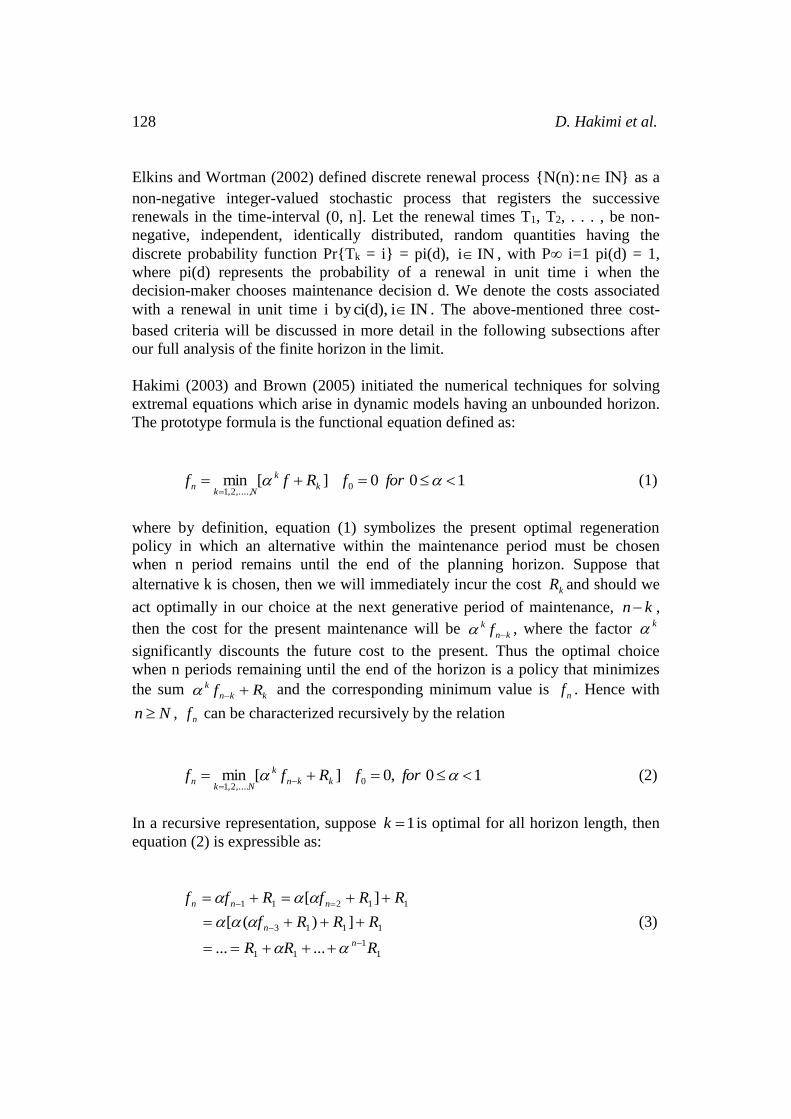
Hakimi (2003) and Brown (2005) initiated the numerical techniques for solving

extremal equations which arise in dynamic models having an unbounded horizon.

The prototype formula is the functional equation defined as:

100][min 0,....,2,1

forfRff k

k

Nkn (1)

where by definition, equation (1) symbolizes the present optimal regeneration

policy in which an alternative within the maintenance period must be chosen

when n period remains until the end of the planning horizon. Suppose that

alternative k is chosen, then we will immediately incur the cost kR and should we

act optimally in our choice at the next generative period of maintenance, kn ,

then the cost for the present maintenance will be kn

k f , where the factor k

significantly discounts the future cost to the present. Thus the optimal choice

when n periods remaining until the end of the horizon is a policy that minimizes

the sum kkn

k Rf and the corresponding minimum value is nf . Hence with

Nn , nf can be characterized recursively by the relation

10,0][min 0,....2,1

forfRff kkn

k

Nkn (2)

In a recursive representation, suppose 1k is optimal for all horizon length, then

equation (2) is expressible as:

1

1

11

1113

11211

......

])([

][

RRR

RRRf

RRfRff

n

n

nnn

(3)


Equation (3) is a useful model for the computation of finite horizon bounded

combinatorial optimization problems. The generality of this model is extensible

into the unbounded horizon.

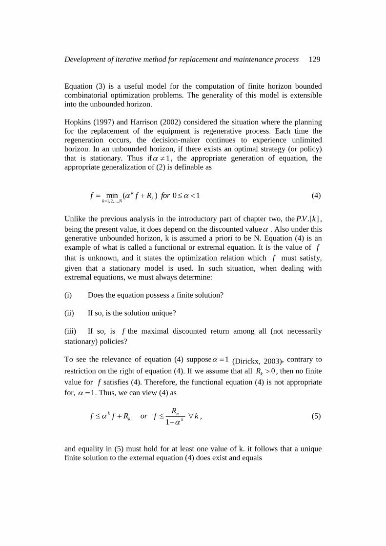
Hopkins (1997) and Harrison (2002) considered the situation where the planning

for the replacement of the equipment is regenerative process. Each time the

regeneration occurs, the decision-maker continues to experience unlimited

horizon. In an unbounded horizon, if there exists an optimal strategy (or policy)

that is stationary. Thus if 1 , the appropriate generation of equation, the

appropriate generalization of (2) is definable as

10)(min,...,2,1

forRff k

k

Nk (4)

Unlike the previous analysis in the introductory part of chapter two, the ].[. kVP ,

being the present value, it does depend on the discounted value . Also under this

generative unbounded horizon, k is assumed a priori to be N. Equation (4) is an

example of what is called a functional or extremal equation. It is the value of f

that is unknown, and it states the optimization relation which f must satisfy,

given that a stationary model is used. In such situation, when dealing with

extremal equations, we must always determine:

(i) Does the equation possess a finite solution?

(ii) If so, is the solution unique?

(iii) If so, is f the maximal discounted return among all (not necessarily

stationary) policies?

To see the relevance of equation (4) suppose 1 (Dirickx, 2003), contrary to

restriction on the right of equation (4). If we assume that all 0kR , then no finite

value for f satisfies (4). Therefore, the functional equation (4) is not appropriate

for, 1 . Thus, we can view (4) as

kR

forRffk

nk

k

1

, (5)

and equality in (5) must hold for at least one value of k. it follows that a unique

finite solution to the external equation (4) does exist and equals


k

k

Nk

Rf

1min

,...,3,2,1 (6)

An optimal stationary policy corresponds to any Alternative k that yields the

optimal value for f The derivation of (6) is also possible on the basis of

stationarity. Since it is optimal to employ the same Alternative k every time a

regression occurs, the present value of the policy is

k

kk

k

k

k

k

k

k

k

k

RRRRRR

1........432

(7)

Thus an optimal policy is the one that minimizes this quantity, as indicated in

equation (6). Hence infinite has been solved using 1 .

Method and Material

This subsection initiates the numerical technique for solving extremal equations

that arise in dynamic programming models having an unbounded horizon. Using

the prototype functional model from equation (4), Winston (1994) and Cani

(2004) said there are three (3) models that can be exploited based on ideas.

(1) The first model estimates from the dynamic context of the underlying

model. The principal conception is to visualize whether a policy which is optimal

for a very long, but finite horizon yields a solution value for f , when used over

unbounded horizon.

(2) The second idea is to guess a value for f . Then compute the quantity on

the right-hand side of equation (4) using the guess value to whether the equation is

satisfied. Otherwise, let the result of the computation be the revised guess and

then repeat the process.

(3) The third model is to guess a policy that may be optimal over an

unbounded horizon. Then solve for the corresponding present value, and use it as

a trial value for f to see if the (4) is satisfied; otherwise, let the new guess value

be the policy which gives minimum on the right-hand side of (4) and repeat the

process ad-infinitum until optimal policy attainment is accomplished.

In these guess methods, each guess can be viewed as an approximation to the

solution, in other words, the solutions are derived from heuristic processes. If the

guess satisfied the extremal equation, it is done. If not, one must guess again. The

iterative process is given the label successive approximations. We now consider

the three models within sequential contexts:


Derman and Klein (2005); and Karp and Held (2007) identify some obvious

approaches for finding a policy which yields a solution to the functional equation

(4). It is to solve the finite horizon model

10,0][min 0,....2,1

forfRff kkn

k

Nkn (8)

for every large value of n. It is significant that for the regeneration model there

exists a finite value x such that for any finite horizon nn , if

nnn k

kn

kkn

kn

n RffthenRff , (9)

KKn

K

K

K RffthenRff , (10)

Equation (8) stipulates that any strategy nk which is optimal for the current

decision when the horizon n is large [greater than n ] is also an optimal stationary

strategy for an unbounded horizon. Model (9) asserts the reverse proposition. By

performing the calculations on model (1) according to a certain computation

format, one can ascertain n . The details of the approach are extraneous of the

purpose of this discussion, and therefore are omitted.

This subsection is to successively approximate the function ,f in the extremal

equation. Hence the idea is the process termed value iteration Denardo (1992).

Suppose we let 0f be the initial approximation, then the technique is to compose

a sequence of approximations ,...,, 210 fff , according to the recursion

10][min,...,3,2,1

1

forRff n

nk

Ni

n (11)

where nf is the trial value for f from iteration n. If the approximation in the

extremal equation indicates “maximization”, then the corresponding change is

made in equation (1). Here, we give an example of the method. Although the

algorithm is well positioned, three questions arise about its applications:

(i) Does the value of nf always approach the value of f that satisfies the

extremal equation?

(ii) If so, is there a finite n such that nf equals f ?


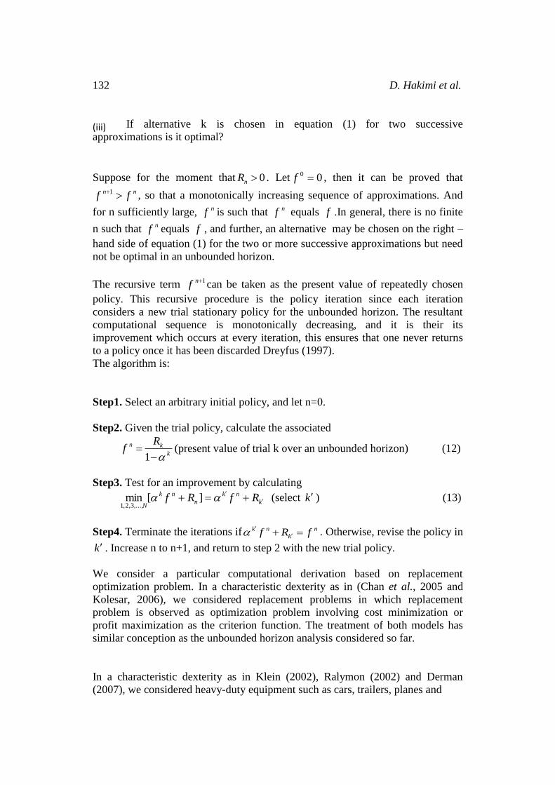
(iii) If alternative k is chosen in equation (1) for two successive

approximations is it optimal?

Suppose for the moment that 0nR . Let 00 f , then it can be proved that

nn ff 1 , so that a monotonically increasing sequence of approximations. And

for n sufficiently large, nf is such that nf equals f .In general, there is no finite

n such that nf equals f , and further, an alternative may be chosen on the right –

hand side of equation (1) for the two or more successive approximations but need

not be optimal in an unbounded horizon.

The recursive term 1nf can be taken as the present value of repeatedly chosen

policy. This recursive procedure is the policy iteration since each iteration

considers a new trial stationary policy for the unbounded horizon. The resultant

computational sequence is monotonically decreasing, and it is their its

improvement which occurs at every iteration, this ensures that one never returns

to a policy once it has been discarded Dreyfus (1997).

The algorithm is:

Step1. Select an arbitrary initial policy, and let n=0.

Step2. Given the trial policy, calculate the associated

k

kn Rf

1(present value of trial k over an unbounded horizon) (12)

Step3. Test for an improvement by calculating

k

nk

n

nk

NRfRf

][min

,...,3,2,1 (select k ) (13)

Step4. Terminate the iterations if n

k

nk fRf

. Otherwise, revise the policy in

k . Increase n to n+1, and return to step 2 with the new trial policy.

We consider a particular computational derivation based on replacement

optimization problem. In a characteristic dexterity as in (Chan et al., 2005 and

Kolesar, 2006), we considered replacement problems in which replacement

problem is observed as optimization problem involving cost minimization or

profit maximization as the criterion function. The treatment of both models has

similar conception as the unbounded horizon analysis considered so far.

In a characteristic dexterity as in Klein (2002), Ralymon (2002) and Derman

(2007), we considered heavy-duty equipment such as cars, trailers, planes and


motor cycles to have their services exponentially distributed over some epoch of

time. Besides the initial cost of the purchase, other contemporaneous costs are

sustained annually for running, maintenance and repairs. These concomitant costs

tend to rise as the equipment gets older. Hence, it is essential over this pressure to

know the most despicable moment to replace the existing equipment with some

new one. This essentially is a replacement fundamental problem.

Ching (1998) and Ching et al. (2004 and 2005) deduced intuitively that the

replacement problem may be conceived or seen as one of knowing when the

running/ maintenance cost becomes so high that the discounted total value is

higher than the cost of buying a new machine. Now let us define their theoretical

model:

(1) An entrepreneur would not have bought equipment in the first place if it would

not pay him to buy it.

(2) He would not want to replace the machine if it would not pay to replace it.

Assumptions (1) and (2) imply that the entrepreneur is rational and the

expectation of profitability in the use of equipment is assumed.

(1) Once the equipment is brought into use, continued profitability of use is

assumed.

(2) An equipment when due for replacement, would be replaced with identical

one.

(3) The equipment is required for an indefinite number of future periods; that is an

equipment is required over an unbounded horizon.

We also considered the following parameters:

yearsnofperiodaover

periodatsfutureallofvaluepresentcumulativeTotalPn cos)(

.cosint/ tperiodinequipmentoftenancemaRunningRt

ratediscountTher

ederbetoiswhichperiodtreplacemenOptimumn mindet

equipmentofpricepurchaseialC int

With the defined parameters, we obtained the model:

13

4

2

321

)1(.......

)1()1()1(

n

nn

r

R

r

R

r

R

r

RRCP

(14)


Thus the present value of all future costs a period is identical to equivalent

discounted value such as (14) is defined as

n

n

n RRRRCP 1

3

2

21 ....... (15)

Where 1)

100

%1(

i

is the discounted factor.

Equations (15) may be written compactly as

i

n

i

i

n RCP

1

1 (16)

That is all cost are discounted to the initial horizon t=1

nP is the anticipated amount that would be needed to replace the equipment after

some period of unforeseeable future. In other words, it could be seen as the total

amount that is needed to purchase and maintain the current piece of equipment

over an unbounded horizon. In optimization subtext, Pn is the optimal amount that

is needed to replace the equipment over an unbounded horizon (Jewell, 2003).

Obviously, Pn may be viewed as the amount of money on hand at the end of the

optimal unbounded horizon or n years when new equipment shall be ready for

procurement or replacement. This computational present amount is short circuited

if we can idealize a fixed nominal amount of money which in financial parlance is

known as annuity or discount value. This value may be contrived in sequential

order as “αt” naira which is set aside each year, will be exactly equal, in

discounted value, to Pn. That is, we need

nn

n

i

t P

........321

1 (17)

The model is derived in a clear exposition:

1

1

2

13

1211

)1(,,.........

)1(,

1,

nnrrr

(18)

Settingv

r

1

1, we can express (17) explicitly as

n

nn

i

t PVVVVV

1

1

4

1

3

1

2

111

1

..... (19)


This can be simplified to;

V

V n

t1

)1(1 (20)

from which the amortized present value can be evaluated.

From equation (20), we can deduce that α1 is the nominal amount of money which

can be saved every year so that, given an annual discount rate “r”, the

accumulated sum after n years will just be enough to purchase a new equipment

and run the new equipment for a subsequent period of n years.

Now comparing equations (17) and (20), we obtained that

)1(

)1(1 nn

V

VP

(21)

The next step is to compute the minimum annuity that can be set aside over the

unbounded horizon such that its accumulative present value would be equal to Pn.

This clearly is the problem of minimizing positive with respect to n years.

Logically, since (1-V) in equation (21) is a constant, whenever (21) is minimized,

it could be conspicuously seen that )1( n

n

V

p

Hence, it is possible to minimize equation (21) to the optimal function such that it

is expressible as:

)1()(

n

n

V

pnF

(22)

with respect to the unbounded period n.

Now that n is a discrete variable, the first-order condition for a minimum can be

attained by the method of finite differences.

F(n) is minimized when

0)1()()1( nFnFnF

(23)

and

0)()1()( nFnFnF

(24)

or, combining the two conditions, when


)(0)1( nFnF (25)

From equation (22),

)1()1()(

1

1

n

n

n

n

V

p

V

pnF

(26)

Upon expansion, equation (2.26) yields

)1)(1(

)1()(

1

)1()(

1

)(

nn

n

n

n

n

n

VV

PVPVPnPnF

(27)

But by definition,

n

n RVRVVRRCnP 1

3

2

21 ........)( (28)

and

1

1

3

2

21 ........)1(

n

n

n

n RVRVRVVRRCnP (29)

Thus

1)()1( n

n

nN RVpp (30)

Hence

n

nnnnn

n

n RVRVRVRVCVPV 2

3

3

2

2

1

11

)(

1 ...... (31)

1

212

3

2

2

1

1)1( ......

n

n

n

nnnnn

n

n RVRVRVRVRVCVPV (32)

Further

1

2

1

111

)1()(

1 )()(][

n

n

t

n

i

tnnnn

n

n

n

n RVRVVVVVCPVPV (33)

which, by re-arrangement,

1

211 )])([(

n

n

t

tnn RVRVCVV (34)

but )(

1 )( nt

t PRVC , therefore

1

2

)(

1

)1()1(

1 )(][

n

n

n

nn

n

n

n

n RVPVVPVPV (35)


By substituting equation (35) and (33) into equation (27) and re-arranging, we

have:

)1)(1(

)()1(1

1

1)( nn

n

nnn

n

n

nVV

PVVVRVF

(36)

which, by further simplification and re-arrangement, gives

nnnn

n

n PV

VR

V

VF

1

1

111)( (37)

By definition, 1V , hence equation (37) can be rewritten as

nnnn

n

n PV

VR

V

VF

1

1

111)( (38)

Considering equation (26), we expression (38) in this manner

01

1

111)(

nnnn

n

n PV

VR

V

VF (39)

Since 1V , 11 n

n

V

Vin equation (39) is always positive.

Hence the inequality in (39) still holds without it. So we drop it and we are left

with the result:

01 1)(

nn

n

n PV

VF (40)

Or, by multiplying each term by V

V n

1

1, we have:

01

11

nn

n

PRV

V (41)

Or


nn

n

PRV

V

1

1

1 (42)

Or

nnn

V

VPR

1

11 (43)

Equation (42) or (43) represents the first condition in equation (26) that 0 nF .

The second condition that 0 nF can similarly derived and shown to be

01

11

1

nn

n

PRV

V (44)

or,

1

1

1

1

nn

n

PRV

V (45)

Equations (42) and (45) are the two basic formulae that are jointly required in the

identification of optimum replacement unbound horizon at period n. They are

interpreted in the following ways:

(1) As long as relation (45) holds, it is not time to replace the equipment.

However, the equipment should be replaced in period n in which the relation (26)

holds. That is, we replace only when

nn

n

PRV

V

1

1

1

And, further, since equation (45) will continue to hold until equation (48) holds, it

is only equation (42) which we really have to look out for in identifying an

optimal replacement period. Finally, we noted that equations (42) and (43) are

equivalent and, as such, either of them can be applied.

Illustration

The purchase value of a machine is #10, 000. 00. The running/ maintenance cost

is estimated at #1, 000.00 per annum for the first five-years, increasing by #300 in

the sixth and the subsequent years. If the prevailing rate of interest is 10 percent

per annum:

(1) When is the optimum time (n) to replace the machine?


(2) What amount of money should be set aside each year for the replacement of

the machine with a new one?

Computational Solution

With the application of equation (42), the model gives Table 1 as solution. It

shows that the machine should be replaced at the end of 11 years:

Table 1: Solution to the Replacement machine

)(t

Year

CInitial

cost

tR

Maint

enanc

e cost

V1 Discoun

t cost

nV1 nth cost

factor

1tV (t-1)

period

cost

factor

t

t RVC 1

present

maintenan

ce cost

t

t

n RVCP 1

present Total

(cumulative)

cost value

1

1

)1(

)1(

t

n

RV

V

Present

cumulative

maintenance

cost value

1 10000 1000 0.0909 0.0909 1.0000 11000.00 11,000.00 1000.00

2 0 1000 0.0909 0.1736 0.9091 909.10 11,909.10 1909.79

3 0 1000 0.0909 0.2487 0.8264 826.40 12,375.50 2735.97

4 0 1000 0.0909 0.3170 0.7513 751.30 13,486.80 3487.35

5 0 1000 0.0909 0.3791 0.6830 683.00 14,169.80 5421.67

6 0 1300 0.0909 0.4355 0.6209 807.17 14,976.97 7665.57

7 0 1600 0.0909 0.4868 0.5645 903.20 15,880.17 10175.14

8 0 1900 0.0909 0.5335 0.5132 975.08 16,855.25 12911.99

9 0 2200 0.0909 0.5759 0.4665 1026.30 17,881.55 15838.83

10 0 2500 0.0909 0.6145 0.4241 1060.25 18,941.80 18928.49

11* 0 2800 0.0909 0.6495 0.3855 1079.40 20,021.20 22150.17

12 0 3100 0.0909 0.6814 0.3505 1086.55 21,107.75 25486.91

13 0 3400 0.0909 0.7103 0.3186 1083.24 22190.99

An alternative replacement model for the machine may be computed using

equation (43):

nnn

V

VPR

1

11

Therefore, an alternative Computation is given in Table 2 as follows:


Table 2: Alternative Iterative Computation

)(t

Year

nV nth

Discou

nt

factor

nV1

nth

cost

facto

r

V1 Discou

nt

Cost

(consta

nt)

)1(

)1(nV

V

Amortizati

on factor

)1(

)1(nn

V

VP

Present cumulative cost

1nR

Present

Cumulati

ve

maintena

nce cost

1 0.9091 0.909 0.909 1.000 11000.00 1000

2 0.8264 0.173

6

0.0909 0.5236 6235.60 1000

3 0.7513 0.248

7

0.0909 0.3655 4654.83 1000

4 0.6830 0.317

0

0.0909 0.2868 3868.01 1000

5 0.6209 0.379

1

0.0909 0.2398 3397.92 1000

6 0.5645 0.435

5

0.0909 0.2087 3125.69 1300

7 0.5132 0.486

8

0.0909 0.1867 2964.83 1600

8 0.4665 0.533

5

0.0909 0.1703 2870.45 1900

9 0.4241 0.575

9

0.0909 0.1578 2821.71 2200

10 0.3855 0.614

5

0.0909 0.1479 2801.49 2500

11 0.3505 0.681

4

0.0909 0.1340 2682.84 2800

12 0.3186 0.710

3

0.0909 0.1334 2815.77 3100

13 0.2897 0.736

7

0.0909 0.1280 2840.45 3400

In order to develop Inventory model over an unbounded horizon, we let:

x , be defined as the production quantity

)(xC , be cost of producing quantity, x, in each period,

)( jh , the cost of holding the inventory at the end of period

d , a constant demand at each period

, be the one-period discount factor; 10 .


Then the appropriate dynamic programming recursion; or the present value for a

finite horizon can be defined as:

10)];()()([min)( 1 dixfdixhxCimizeif nx

n (46)

Equation (46) is expressible as an extremal function as

10)];()()([min)( dixfdixhxCimizeifx

(47)

Equation (47) expresses a system of equations over an unbounded horizon. In

equation (47), if is conceived as the present value of an optimal policy over an

unbounded horizon, given the inventory entering the current period is i . So

equation (47) is now our new inventory model.

Hitherto, the inventory equation in use is:

48,1

tt

N

t

t ixCMinimize

Where:

tx production quantity in period t

ti inventory at the end of period t

ttt ixC , cost of incurring quantity x at period t which depends only on the

production quantity tx and the ending inventory level ,ti and on period t.

Now, the inventory model (48) only balanced off manufacturing with inventory

holding costs. The economic cost of varying production levels from one period to

the next was ignored and the model equally ignored discount factor knowing fully

that money depreciates with time. All these deficiencies are taken cared by our

newly developed inventory model.

Discussion of Results

From Table 1, the optimal period n=11 and is starred * since it is at this period of

time, that the present cumulative maintenance cost is higher than the present

cumulative cost which is the optimal value amount that shall be needed on the 11th

year. The actual money to set aside during the twelve years:


20.20021*6495.0

0909.0

)1(

)1(111111

P

V

V

annumper04.2802#

20.20021*13995381.0

However, from Table 2, the optimal period is n = 11 since at this period of time, it

is observed that the present cumulative maintenance cost is higher than the present

cumulative cost. At this point in time, it is advised that the machine or whatever is

being maintained; be stopped. Any further maintenance would result to loss, so

the maintaining article should be replaced with a new one.

Conclusion

This paper has been quite illuminating. Many computational models based on

finite and infinite models; known respectively as bounded and unbounded

horizons, have been numerically computed through various models. We

developed iterative method for replacement and maintenance process using

inventory model and they are very efficient even for large systems unlike the

existing exhaustive enumeration algorithm which can be used only if the number

of stationary policies is reasonably small.

Recommendations

Due to the importance of inventory in business, we developed and applied

deterministic inventory model. So, we recommend that interested researchers

should consider the case of developing probabilistic inventory model over

unbounded horizon.

References

[1] Blackwell, D. (2002), Discounted Dynamic Programming, Annals

Mathematical Statistics, Vol. 93, pp. 93-99.

[2] Brown, B. (2005), On the Iterative Method of Dynamic Programming on a

Finite Space Discrete Time Markov Process, Annals Mathematics Statistics, Vol.

96, pp. 226-235.

[3] Cani, J. S. (2004), A Dynamic Programming Algorithm for Embedded

Markov Chains When the Planning Horizon is at Infinity, Management Science,

Vol. 110, pp. 716-733.


[4] Chan, R., Ma, K. and Ching, W. (2005), Boundary Value Methods for Solving

Transient Solutions of Markovian Queueing Networks, Journal of Applied

Mathematics and Computations. http://dx.doi.org/10.1016/j.amc.2004.11.014

[5] Ching W. (1998), Iterative Methods for Manufacturing Systems of Two

Stations in Tandem, Applied Mathematics Letters, Vol. 11, pp. 7-12.

http://dx.doi.org/10.1016/s0893-9659(97)00124-9

[6] Ching W., Fung E. and Ng M. (2004), Building Higher-order Markov Chain

Models with Excel, International Journal of Mathematical Education in Science

and Technology, Vol. 35: pp 921-932.

http://dx.doi.org/10.1080/00207390412331271302

[7] Ching W., Ng M., Fung E. and Siu T. (2005), An Interactive Hidden Markov

Model for Categorical Data Sequences, Working paper.

[8] Cho D. and Parlar M., (1991), A survey of Maintenance Models for Multi-unit

Systems, European Journal of Operational Research, Vol. 51, pp 1-23.

http://dx.doi.org/10.1016/0377-2217(91)90141-h

[9] Denardo, E. (1992), Dynamic Programming Theory and Applications, Prentice

Hall, Upper Saddle River, NJ.

[10] Denardo, E. V., and B. I., Miller (2008), An Optimality Condition for

Discrete Programming with no Discounting, Annals Mathematical Statistics, Vol.

99, pp. 1220-1227.

[11] Derman, C. and M. Klein (2005), Some Remarks on Finite Horizon

Markovian Decision Models, Operation Research, Vol. 111, pp. 272-278.

[12] Derman, C. (2007), Optimal Replacement and Maintenance under Markovian

Deterioration with Probability Bounds on Failure, Management Science, Vol. 113,

pp. 478-481.

[13] Dirickx, Y. M. I. (2003), Deterministic Discrete Dynamic Programming with

Discount Factor Greater than one: Structure of Optimal Policies, Management

Science, pp. 32-43.

[14] Dreyfus, S. (1997), The Art and theory of Dynamic Programming, Academic

Press, Newyork.

[15] Elkins D.A. and Wortman M.A. (2002), On Numerical Solution of Markov

Renewal Equation:Tight Upper and Lower Bounds, Methodology Computation

Application Probability, Vol.3, pp 239-253.

http://dx.doi.org/10.1016/j.amc.2004.11.014

http://dx.doi.org/10.1016/s0893-9659%2897%2900124-9

http://dx.doi.org/10.1080/00207390412331271302

http://dx.doi.org/10.1016/0377-2217%2891%2990141-h


[16] Hakimi, D. (2003), Optimization Algorithm for an Unbounded Horizon;

M.Tech. Thesis, Federal University of Technology, Minna, Nigeria.

[17] Hakimi, D., (2011), Development of Mathematical models for problems of

unbounded horizon using both deterministic and stochastic processes; P.hD.

Thesis, Federal University of Technology, Minna, Nigeria.

[18] Harrison, M. (2002), Discrete Dynamic Programming with Unbounded

Rewards, Annals Mathematical Statistics, Vol. 93, pp. 636-644.

[19] Hopkins, D. S. P. (1997), Infinite-Horizon Optimality in an Equipment

Replacement and Capacity Expansion Model, Management Science, Vol. 18, pp.

145-156.

[20] Jewell, W. S. (2003), Markov-Renewal Programming I, II, Operation

Research, Vol. 103, pp. 938-971.

[21] Kolesar, P. (2006), Minimum Cost replacement under Markovian

Deterioration, Operation Research, Vol. 112, pp. 694-706.

[22] Mode C. J. and Pickens, G.T. (1998), Computational Methods for Renewal

Theory and Semi-markov Processes with Illustrative Examples, Amer. Statis, Vol.

42 No.2, pp 143-152.

[23] Noortwijk, S. and Peerbolta, F. Y. (2000), Managing Repairable Item

Inventory Systems: A Review in TIMS Studies, Management Science, 16: pp

252-277.

[24] Tersine R. (1998), Principles of Inventory and Materials Management, Third

Edition, North Holland, New York.

[25] Winston W. (1994), Operations Research: Applications and Algorithms,

Belmont CA, Third Edition, Duxbury Press.

[26] Waters C., (1992), Inventory Control and Management, Wiley, New York.

Received: November 1, 2014; Published: December 23, 2014

Documents

Development of Iterative Method for Replacement and Maintenance …m-hikari.com/ijco/ijco2014/ijco1-4-2014/waziriIJCO1-4... · 2015-01-11 · Development of Iterative Method for Replacement