Embed Size (px)
Citation preview

Filipe Tiago Alves de Magalhães
Development of gas detection systems based on microstructured optical fibres
Thesis submitted to Faculdade de Engenharia da Universidade do Porto in partial fulfilment of the requirements for the degree of Master in Engenharia Electrotécnica e de Computadores
Faculdade de Engenharia da Universidade do Porto Departamento de Engenharia Electrotécnica e de Computadores
Rua Roberto Frias, s/n, 4200-465 Porto, Portugal
March/2008

Development of gas detection systems based on microstructured optical fibres
Filipe Tiago Alves de Magalhães
Thesis supervised by
PhD Henrique Manuel de Castro Faria Salgado Associate Professor of Departamento de Engenharia Electrotécnica e de Computadores of
Faculdade de Engenharia da Universidade do Porto
and by
PhD Luís Alberto de Almeida Ferreira Senior Researcher at Optoelectronics and Electronic Systems Unit – UOSE
INESC Porto
_____________________________________________________ (President of the Jury, PhD Manuel Alberto Pereira Ricardo)

“Estudar é uma coisa em que está indistinta A distinção entre nada e coisa nenhuma.”
Liberdade, Fernando Pessoa
iii

Acknowledgements First of all I would like to thank Dr. Luís Ferreira for giving me the opportunity to enter the fascinating world of scientific research and for making this project such a pleasant experience. Thank you for all the patience and key insights. I’m also grateful to Dr. Henrique Salgado for having accepted this project and for all the time and effort spent in reviewing this manuscript. A word of appreciation is also directed to Joel Carvalho for being a good partner and for the shared knowledge. To all the UOSE team I would like to thank for the enjoyable working atmosphere. I would like to thank Dr. Jonathan Knight and Rodrigo Correa, from the University of Bath, for providing the photonic crystal fibres used in the experiments. To my parents, for being a source of endless love and support, I would like to express my deepest gratitude. To Joana I want to thank for always being present and to say I am sorry for all the quality time we have lost. At last, I would like to thank INESC Porto for the grant provided and the NextGenPCF project, supported by the Sixth Framework Programme, for the funding provided.
iv
Abstract The main goal of this project was to study and develop sensing systems for the remote detection of gases with the use of microstructured optical fibres of the hollow-core type (HC-PCF) and the use of signal processing techniques usually associated with absorption spectroscopy. After studying the common methodologies for this type of monitoring many drawbacks were identified, among which were the need for long interaction path lengths and high sampling volumes, the need for precise alignments and optics and the sensitivity to power fluctuations. Photonic Crystal Fibres (PCF) arose as an exceptionally interesting player in the field of gas sensing since they promote the creation of short and direct interaction paths between light and gas and can be tuned to address any specific gas. Thus, their principle of operation and main optical properties were studied and described. The diffusion time of gases inside of microstructured fibres is a subject of special importance if we intend to use these fibres as sensing heads. As a consequence of its theoretical study and experimental analysis, fruitful results for the planning of a new configuration for the sensing head were achieved. Light coupling between standard optical fibres and hollow-core photonic crystal fibres is a practical issue that was also evaluated in the aim of the work here presented. The splice between these two types of fibres was also optimized. Wavelength Modulation Spectroscopy is a powerful and sensitive technique for gas detection given that detection is shifted to frequencies far from the base-band noise, improving the signal-to-noise ratio. Consequently, it was the chosen signal processing technique to be used in the implementation of an experimental setup for the detection and monitoring of a specific gas species. The implementation of a portable and compact unit for remote gas monitoring, involving several of the aspects here approached, has already been initiated.
v
Resumo O objectivo principal deste projecto era o estudo e o desenvolvimento de sistemas sensores para detecção remota de gases com recurso a fibras ópticas microestruturadas do tipo hollow-core e a técnicas de processamento de sinal normalmente associadas à espectroscopia de absorção. Após as metodologias mais comuns para este tipo de monitorização terem sido estudadas várias insuficiências foram identificadas, entre as quais estavam a necessidade de comprimentos de interacção longos e de grandes volumes de amostra, a exigência de alinhamentos ópticos de precisão e a sensibilidade a flutuações de potência. As Fibras de Cristais Fotónicos revelaram-se extremamente interessantes para a área da detecção de gases uma vez que possibilitam a criação de segmentos curtos de interacção directa entre a luz e os gases e também porque podem ser desenvolvidas para endereçarem um gás especifico. Assim, o seu princípio de funcionamento e as suas principais propriedades ópticas foram estudadas e descritas. O tempo de difusão de gases no interior de fibras microestruturadas constitui um assunto de particular relevância se desejarmos usar estas fibras como cabeças sensoras. Como consequência do seu estudo teórico e análise experimental, foram atingidos resultados proveitosos para a idealização de uma nova configuração para a cabeça sensora. O acoplamento de luz entre as fibras convencionais e as fibras do tipo hollow-core é uma questão prática que também foi avaliada no âmbito do trabalho aqui apresentado. A fusão destes dois tipos de fibras também foi optimizada. A Espectroscopia por Modulação de Comprimento de Onda é uma técnica poderosa de elevada sensibilidade para a detecção de gases dado que a detecção é deslocada para frequências afastadas do ruído de base, melhorando assim a relação sinal-ruído. Consequentemente, esta foi a técnica de processamento de sinal escolhida para ser usada na implementação de uma montagem experimental para detecção e monitorização de um gás específico. A implementação de uma unidade portátil e compacta para monitorização remota de gases, envolvendo vários dos aspectos aqui abordados, já foi iniciada.
vi

Contents
Acknowledgements ......................................................................................................................... iv Abstract ................................................................................................................................................ v Resumo ...............................................................................................................................................vi Contents .............................................................................................................................................vii List of figures..................................................................................................................................... ix 1 Introduction ...............................................................................................................................1
1.1 Thesis structure ..................................................................................................................1 1.2 Motivation...........................................................................................................................1 1.3 Contributions......................................................................................................................3 1.4 Publications.........................................................................................................................3
2 Optical Sensing Techniques for Gas Sensing.................................................................. 4 2.1 Introduction........................................................................................................................4 2.2 Methane sensing setups.....................................................................................................4 2.3 Photonic crystal fibers in gas sensing technology .........................................................9 2.4 Pellistors in gas sensing technology ..............................................................................10 2.5 Summary............................................................................................................................11
3 Photonic Crystal Fibres ........................................................................................................12 3.1 Introduction......................................................................................................................12 3.2 Brief overview ..................................................................................................................12 3.3 Light Guidance in Solid-Core PCF ...............................................................................12 3.4 Light Guidance in Hollow-Core PCF...........................................................................14 3.5 PCF Fabrication ...............................................................................................................15 3.6 Optical Properties ............................................................................................................17
3.6.1 Modal Properties .........................................................................................................17 3.6.2 Chromatic Dispersion.................................................................................................17 3.6.3 Attenuation...................................................................................................................18
3.7 Summary............................................................................................................................19 4 Wavelength Modulation Spectroscopy ............................................................................20
4.1 Introduction......................................................................................................................20 4.2 Definition..........................................................................................................................20 4.3 Mathematical analysis ......................................................................................................22 4.4 Simulation results .............................................................................................................25 4.5 Summary............................................................................................................................27
5 Evaluation of coupling losses between SMF and HC-PCF.......................................29 5.1 Introduction......................................................................................................................29 5.2 Modelling approach .........................................................................................................29 5.3 Experimental results ........................................................................................................31 5.4 Summary............................................................................................................................38
6 Detection Scheme ..................................................................................................................39 6.1 Introduction......................................................................................................................39 6.2 Experimental Setup .........................................................................................................39
6.2.1 Gas chamber ................................................................................................................42 6.2.2 Choice of the laser source ..........................................................................................43 6.2.3 Software ........................................................................................................................46
vii

6.3 Characterization of the detection scheme ....................................................................48 6.3.1 Gas-cells characterization...........................................................................................48 6.3.2 Results invariance in the presence of power fluctuations .....................................50 6.3.3 Feedback-loop response to perturbations ...............................................................51 6.3.4 Laser power modulation.............................................................................................52
6.4 Results................................................................................................................................53 6.5 Summary............................................................................................................................56
7 Diffusion time of gases inside of HC-PCF.....................................................................57 7.1 Introduction......................................................................................................................57 7.2 Theoretical analysis ..........................................................................................................57 7.3 Experimental Results.......................................................................................................61 7.4 Summary............................................................................................................................67
8 Portable Monitoring Unit ....................................................................................................68 8.1 Introduction......................................................................................................................68 8.2 Distributed Sensing Alternatives ...................................................................................70
9 Conclusions..............................................................................................................................72 10 Appendixes...............................................................................................................................73 A Poster accepted for the European Workshop on Optical Fibre Sensors – 2007.................73 B Poster accepted for the Symposium on Enabling Optical Networks and Sensors – 2007.74 C Oral presentation on Symposium on Enabling Optical Networks and Sensors – 2007 .....75 11 References ................................................................................................................................85
viii

List of figures Figure 1 - Global monthly methane concentration in parts per billion (ppb). [1]......................2 Figure 2 – Methane absorption spectrum (from HITRAN) .........................................................4 Figure 3 – Remote detection of methane in air (transmission scheme).......................................5 Figure 4 – Remote detection of methane in air (reflection scheme) ............................................5 Figure 5 – Methane optical sensor using a 1.31 μm DFB laser and a signal processing
technique which provides auto-calibration.........................................................................6 Figure 6 – Schematic diagram of a portable remote methane sensor based on frequency
modulation using a DFB laser ..............................................................................................6 Figure 7 – (a) Absorption spectra of methane; (b) fundamental frequency (f) signal;
(c) second-harmonic signal (2f) [7] .......................................................................................7 Figure 8 - Diagram of the low-loss fibre-optic remote sensing system for differential
absorption measurements .....................................................................................................7 Figure 9 – Cavity ring-down sensing system....................................................................................8 Figure 10 – Multipass transmission absorption spectroscopy scheme ........................................8 Figure 11 – Photoacoustic spectroscopy diagram...........................................................................8 Figure 12 – Two solid-core holey optical fibres [17] ......................................................................9 Figure 13 – Microscope images of air-guiding photonic bandgap fibres proposed for gas
sensing [19] ..............................................................................................................................9 Figure 14 – Experimental setup used to perform experiments [21]...........................................10 Figure 15 – Pellistor drive/measurement circuit ...........................................................................11 Figure 16 – Light propagation inside a fibre by total internal reflection. As long as θi (angle
of incidence) is greater that θc (critical angle), there are no optical power losses caused by light coupling to the cladding. n1 and n2 (n1>n2) are the refractive indexes of the core and cladding, respectively. ..............................................................................12
Figure 17 – Propagation diagrams for (A) a conventional single-mode fibre with a Ge-doped silica core and a pure silica cladding and for (B) a solid-core PCF. [24] ......................13
Figure 18 – Hollow-core PCF from BlazePhotonics; a) 7-cell PCF (HC-1550-02); b) 19-cell PCF (HC19-1550-01). [25]..................................................................................................14
Figure 19 – Transmission spectra for a 7-cell (HC-1550) and a 19-cell core fiber (HC19-1550), both designed for operation at 1550 nm. [26]......................................................14
Figure 20 – Photonic crystal microstructure found in the wings of Cyanophrys remus butterflies.................................................................................................................................................15
Figure 21 – Optical micrograph exhibiting the near-field of a red mode in a hollow-core PCF, with white light being injected into the core. [26] .................................................15
Figure 22 – Stack-and-draw PCF fibre’s fabrication technique [26]...........................................16 Figure 23 – Typical near field intensity distribution for a 19-cell PCF. [25] .............................17 Figure 24 - Typical attenuation and chromatic dispersion spectrum of a HC19-1550-01 [25]
.................................................................................................................................................17 Figure 25 – Average attenuation calculated from three traces obtained from three ≈ 800 m
fibre samples, in a range close to the minimum attenuation wavelength. [29]............18 Figure 26 - The simplest sensor configuration for measuring changes in optical transmitted
power......................................................................................................................................20 Figure 27 – Wavelength modulation converted to amplitude modulation in Wavelength
Modulation Spectroscopy....................................................................................................20
ix
Figure 28 – Spectral output of a laser beam: a) unmodulated; b) modulated with no absorption; c) modulated with absorption........................................................................21
Figure 29 – WMS output obtained with a lock-in amplifier, locked at dithering frequency (experimental data obtained with the implemented setup). ...........................................21
Figure 30 - Frequency duplication phenomenon, resulting from dithering at the absorption peak.........................................................................................................................................22
Figure 31 – Simple configuration to directly quantify gas absorption .......................................22 Figure 32 – Simulation result for (L=3 cm) ........................................................................25 DC
OUTA
Figure 33 - Simulation result for (L=3 cm).........................................................................26 ω2
OUTA
Figure 34 - Simulation result for DCOUT
OUT
AA ϖ2
(L=3 cm)........................................................................26
Figure 35 - Simulation result for (L=5 cm).........................................................................26 DCOUTA
Figure 36 - Simulation result for (L=5 cm)..........................................................................27 ω2
OUTA
Figure 37 - Simulation result for DCOUT
OUT
AA ϖ2
(L=5 cm).........................................................................27
Figure 38 – Coupling between two fibres separated by distance d.............................................29 Figure 39 – (a) Mode of a 7-cell HC-PCF; (b) Mode of a 19-cell HC-PCF; (c) Radially
averaged mode of a 7-cell HC-PCF; (d) Radially averaged mode of a 19-cell HC-PCF.........................................................................................................................................30
Figure 40 – Radial average of mode profiles for SMF, 7-cell HC-PCF, and 19-cell HC-PCF..................................................................................................................................................30
Figure 41 – (a) Coupling coefficients: SMF → 7-cell HC-PCF, SMF → 19-cell HC-PCF; ...31 Figure 42 - Setup used for the experimental evaluation of the coupling loss between SMF
and HC-PCF. ........................................................................................................................32 Figure 43 – Setup used for the experimental evaluation of the coupling loss between HC-
PCF.........................................................................................................................................32 Figure 44 – Excess loss dependence on axial displacement: (a) between a SMF and 19-cell
HC-PCF, and between two 19-cell HC-PCF; (b) between a SMF and 7-cell HC-PCF, and between two 7-cell HC-PCF. ......................................................................................33
Figure 45 – Comparison of the excess loss dependence on axial displacement between the theoretical and the measured values: (a) SMF → 19-cell HC-PCF; (b) SMF → 7-cell HC-PCF; (c) 19-cell HC-PCF → 19-cell HC-PCF..........................................................34
Figure 46 – Excess loss dependence on lateral displacement: (a) between a SMF and a 19-cell HC-PCF and between a SMF and a 7-cell HC-PCF; (b) between a SMF and a 19-cell HC-PCF, and between two 19-cell HC-PCF. ..................................................................35
Figure 47 – Current (mA) as a function of arc power (bits) for the Fujikura FSM-40S splicing machine ..................................................................................................................................36
Figure 48 - Experimental setup used to estimate the splice losses between a SMF and 19-cell HC-PCF.................................................................................................................................36
Figure 49 – (a) Result of the automatic alignment of the Fujikura’s splicing machine; (b) Result of manual alignment (after this the electric arc is applied).................................37
Figure 50 – Experimental results obtained for estimation of losses in light coupling between SMF and 19-cell HC-PCF in different cases. ...................................................................37
x

Figure 51 – Photographs of the different splices between SMF and 19-cell HC-PCF, showed in Figure 50............................................................................................................................37
Figure 52 – Proposed detection scheme.........................................................................................39 Figure 53 - Gas detection scheme with sensing head substituted by a sealed gas cell.............40 Figure 54 – Setup used to simulate variations in the gas concentration ....................................40 Figure 55 – Simulated variation of gas concentration ..................................................................41 Figure 56 – Variable coupler’s output. It is clearly seen that the total optical power is not
constant..................................................................................................................................42 Figure 57 – Computer generated images and photos of the gas chamber ................................42 Figure 58 – Wavelength variation vs. pumping current for the Avanex 1905 LMI DFB
source. ....................................................................................................................................44 Figure 59 – Wavelength variation vs. pumping current for the NEL DFB source .................45 Figure 60 – Wavelength variation vs. temperature for the NEL DFB source..........................45 Figure 61 – Flowchart of the developed LabVIEW application.................................................46 Figure 62 – Graphical user interface of the developed application............................................47 Figure 63 – Setup used to acquire the absorption spectrum of the gas cells ............................48 Figure 64 – Absorption spectrum of different gas cells using different configurations..........48 Figure 65 – Absorption spectrums of two identical gas cells connected in series and measured in transmission and one of those cells measured in reflection. .................................49 Figure 66 – Setup used to trace the absorption spectrum of the gas cells in reflection ..........49 Figure 67 – Setup with optical variable attenuator to evaluate the influence of power
fluctuations in the sensor signal .........................................................................................50 Figure 68 – Analysis of the influence of power attenuation in the system’s response ............50 Figure 69 – Feedback-loop responses for different gain values..................................................52 Figure 70 – Power and wavelength variation with current modulation.....................................52 Figure 71 – Data experimentally acquired to measure the system resolution (longer U-bench)..............................................................................................................................................................53 Figure 72 - Data experimentally acquired to measure the system resolution (shorter U-bench)..............................................................................................................................................................54 Figure 73 – Setup used to measure the amount of absorbed light by the gas inside of the
chamber .................................................................................................................................54 Figure 74 – Absorption spectrum obtained with the setup of Figure 73 (longer U-bench)...55 Figure 75 - Absorption spectrum obtained with the setup of Figure 73 (shorter U-bench) ..55 Figure 76 – Quarter of the cross section of a PCF fibre. [39].....................................................57 Figure 77 – Relative sensitivities of Lucent’s and the modified Lucent’s PCFs as functions of
wavelength: Lucent’s PCF, Λ=1.55 µm, d=1.4 µm, d/Λ = 0.9; modified PCF, Λ = 1.33 µm and the varying hole diameter corresponding to d/Λ from 0.69 to 0.93. [39].................................................................................................................................................57
Figure 78 – Time-dependence of the average relative methane concentration inside different lengths of HC-PCF, having a single open end.................................................................58
Figure 79 - Time-dependence of the average relative methane concentration inside different lengths of HC-PCF, having two open ends. ....................................................................59
Figure 80 - Time-dependence of the average relative acetylene concentration inside different lengths of HC-PCF, having a single open end.................................................................60
Figure 81 - Time-dependence of the average relative acetylene concentration inside different lengths of HC-PCF, having two open ends. ....................................................................60
Figure 82 - Sensing head with periodic openings in the PCF fibre. ...........................................61 Figure 83 – Setup used to measure the diffusion time of gas inside of HC-PCF ....................61
xi
Figure 84 – Photo of two ferrules connected and aligned by a zirconia sleeve with a slit......61 Figure 85 – Overview of the setup used to align the HC-PCF inside of the ferrules..............62 Figure 86 – Detailed image of the setup used for alignment of the HC-PCF inside of the
ferrules....................................................................................................................................62 Figure 87 – Photo with detailed view of the HC-PCF alignment inside of the ferrule ...........62 Figure 88 – Photo of HC-PCF misaligned with the ferrule.........................................................63 Figure 89 – Photo of the HC-PCF aligned with the ferrule ........................................................63 Figure 90 – Detailed photo of the HC-PCF aligned with the ferrule ........................................63 Figure 91 – Photos taken with a microscope of the HC-PCF position inside of the ferrule:
(a) HC-PCF with an outer diameter of 125 µm; (b) HC-PCF with an outer diameter of 115 µm...............................................................................................................................63
Figure 92 – Sketch of the gap between an 8º angled ferrule and a flat ferrule .........................64 Figure 93 – Experimental results for the diffusion time of 5% of methane inside of a HC-
PCF (with two open ends) ..................................................................................................64 Figure 94 – Microscope photo of the fibre developed for the U-band .....................................65 Figure 95 – Setup used by the IPHT-Jena to analyse the diffusion time of methane inside of
a HC-PCF..............................................................................................................................65 Figure 96 – Experimental results for the diffusion time of 100% of CH4 inside of a HC-PCF
(with two open ends) ...........................................................................................................66 Figure 97 – Wall-effect and temperature effect in the diffusion time of gas inside of different
lengths of HC-PCF ..............................................................................................................66 Figure 98 – 3D computer model of the portable monitoring unit that is being implemented..............................................................................................................................................................68 Figure 99 – Optical-electrical scheme for the interrogation unit ................................................69 Figure 100 – Schematic diagram of the monitoring unit and sensing head for the case of
measurements performed in reflection .............................................................................69 Figure 101 – Optical-electrical board that is being implemented to the portable unit ............70 Figure 102 – Sensors distributed in series along a fibre. ..............................................................70 Figure 103 – Sensors branching from a main fibre with the use of couplers. ..........................71
xii

Introduction
1
1 Introduction
1.1 Thesis structure This thesis is divided in nine chapters as follows:
⎯ Chapter 1 describes the motivation and the thesis structure ⎯ Chapter 2 presents the evolution of optical gas sensing technologies as well as the
use of photonic crystal fibres and pellistors in gas sensing ⎯ Chapter 3 extensively describes photonic crystal fibres and along with their
fabrication process and optical properties ⎯ Chapter 4 gives a description of Wavelength Modulation Spectroscopy and presents
some mathematical and simulated results on this subject ⎯ Chapter 5 gives a detailed description of the evaluation of the coupling losses
between SMF and HC-PCF and presents results for the optimization of splices between these two types of fibres
⎯ Chapter 6 extensively describes the implemented experimental setup as well as its characterization
⎯ Chapter 7 presents the study and the experimental results of the diffusion time of gases inside of HC-PCF
⎯ Chapter 8 shows the idealized portable monitoring unit that is already being implemented
⎯ Chapter 9 ends the thesis with some concluding remarks. Future work suggestions are also given.
1.2 Motivation Methane is an extremely explosive gas and one of the main constituents of natural gas, so its detection is a subject of major importance. Besides natural gas, there are several other sources of emission of this gas, and these can be natural (cattle, gas hydrates in the ocean floor, wetlands …) or directly related to human activity (landfills, mining sites, rice paddies, combustion of fossil fuels …). In addition to its explosiveness, methane is 20 times more powerful than carbon dioxide as a greenhouse gas. Even being less abundant in the atmosphere than CO2, it is more than obvious that its emissions should be well controlled and reduced to its most.

Introduction
Figure 1 - Global monthly methane concentration in parts per billion (ppb). [1]
This project arises from the work being developed at INESC Porto in the aim of a European project called NextGenPCF – Next Generation of Photonic Crystal Fibres (http://www.nextgen-pcf.eu/). NextGenPCF is an application driven research project, seeking the enrichment of Europe’s principal industrial and academic actors in PCF related science and the turning of this excellence into key competitive factors for the European firms. There are three mainstreams:
• biomedical, pursuing the application of PCF in new therapies and in the development of new light sources;
• telecommunications, for the development of easy-to-install, low-cost fibre to fibre to the home, and optical amplifiers;
• sensors for the environment, which is INESC Porto work package, whose main goal is the development of sensing systems for detection of methane gas in mining sites.
Our purposes are focused on several criteria such as compactness (fibre-sized), high sensitivity and an increased flexibility (tuneable to other gas species, tuneable in length, etc). These properties are believed to give an added value to the sensing system and therefore the objectives are set to outperform the current state-of-the-art. From a personal point of view, it was with great pleasure that I embraced this project as an opportunity to further extend my knowledge and to work with a revolutionary type of optical fibres. Being involved in a project with such dimensions has been an extremely fulfilling experience that will certainly contribute to my personal and professional future.
2

Introduction
3
1.3 Contributions
1. Implementation of an experimental setup for gas detection and measurement
through Wavelength Modulation Spectroscopy
2. Evaluation of coupling losses between SMF and HC-PCF
3. Splice optimization between single mode fibres and hollow-core photonic crystal
fibres
4. Implementation of a gas chamber to perform experimental tests with methane and
acetylene
5. Study of the diffusion time of gases inside HC-PCF
6. Design of a compact and portable measurement unit for gas detection
1.4 Publications
• F. Magalhães, J. P. Carvalho, J. L. Santos, F. M. Araújo, L. A. Ferreira. “Implementation of a compact interrogation system for remote detection of methane”, SEON 2007 - V Symposium on Enabling Optical Networks and Sensors, Aveiro, 29th of June, 2007.
• J. P. Carvalho, F. Magalhães, O. Frazão, J. L. Santos, F. M. Araújo, L. A. Ferreira.
“Hollow-core photonic crystal fibres for gas sensing applications”, SEON 2007 - V Symposium on Enabling Optical Networks and Sensors, Aveiro, 29th of June, 2007.
• J. P. Carvalho, F. Magalhães, O. V. Ivanov, O. Frazão, F. M. Araújo, L. A. Ferreira,
J. L. Santos. “Evaluation of coupling losses in hollow-core photonic crystal fibres”, EWOFS 2007 - Third European Workshop on Optical Fibre Sensors, 4th-6th of July, 2007, Napoli, Italy, session III, poster 85.

Optical Sensing Techniques for Gas Sensing
4
2 Optical Sensing Techniques for Gas Sensing
2.1 Introduction This chapter describes the actual state-of-the-art of optical sensing technologies, as well as their major advantages and drawbacks. The emergence of air-guiding photonic band fibres will be reported and their use in this type of applications justified. At the end of this chapter, pellistors, as a widely implemented solution, are also analyzed even though they do not constitute an optical sensing method.
2.2 Methane sensing setups The idea of sensing methane by laser absorption was first proposed in 1961 by Moore [2], and later demonstrated by Grant [3] in 1986 using a He-Ne laser. Although methane has a strong absorption line at 3.3 μm (Figure 2), this wavelength region is not suited for use in optical fibre sensor applications, since it is difficult to fabricate laser diodes operating at wavelengths higher than 2.2 μm at room temperature, and due to the high losses in standard optical fibres. In order to effectively use the currently available low loss optical fibres, remote detection in the near infrared around 1.1-1.8 μm is desirable, where optical fibres have minimum transmission losses (<1 dB/km). Methane has two absorption lines in this region, corresponding to wavelengths of 1.33 μm and 1.65 μm. It was found that the 1.65 μm band of methane absorption is more suitable considering the lower loss of the optical fibre in this region, and also the fact that the absorption coefficients are larger and the spectral widths are broader than those in the 1.33 μm band.
Figure 2 – Methane absorption spectrum (from HITRAN)
Usually, the spectroscopic technique is the only way to provide methane sensing with high sensitivities. Moreover, it has many other advantages such as, fast response time and molecular selectivity. In particular, absorption spectroscopy using tuneable laser sources (diode lasers or fibre lasers) can lead to compact and low-cost remote methane sensors.
3.3 µm
8.3 µm
2.3 µm
1.67 µm

Optical Sensing Techniques for Gas Sensing
Several authors have proposed many configurations using laser diodes, in particular, distributed feedback (DFB) lasers with almost monochromatic emission, having bandwidths much narrower than the individual gas absorption lines. However, these devices are generally quite expensive which could be a significant disadvantage. In 1992, Uehara et al [4] demonstrated high sensitivity real time remote detection of methane in air with a DFB operating at 1.65 μm (transmission and reflection schemes; Figure 3 and Figure 4).
Figure 3 – Remote detection of methane in air (transmission scheme)
Figure 4 – Remote detection of methane in air (reflection scheme)
In the two methods previously depicted the driving current of a single mode laser was modulated at a high frequency, f, of 5.35 MHz and the laser emission was locked to the centre of a methane absorption line by the means of a reference methane cell. Absorption in the probed area was then detected by the output of a lock-in at 2f. Particularly, for the case of the reflection scheme the ratio between the fundamental and second-harmonic signal intensities produced results independent of the received power.
5
Optical Sensing Techniques for Gas Sensing
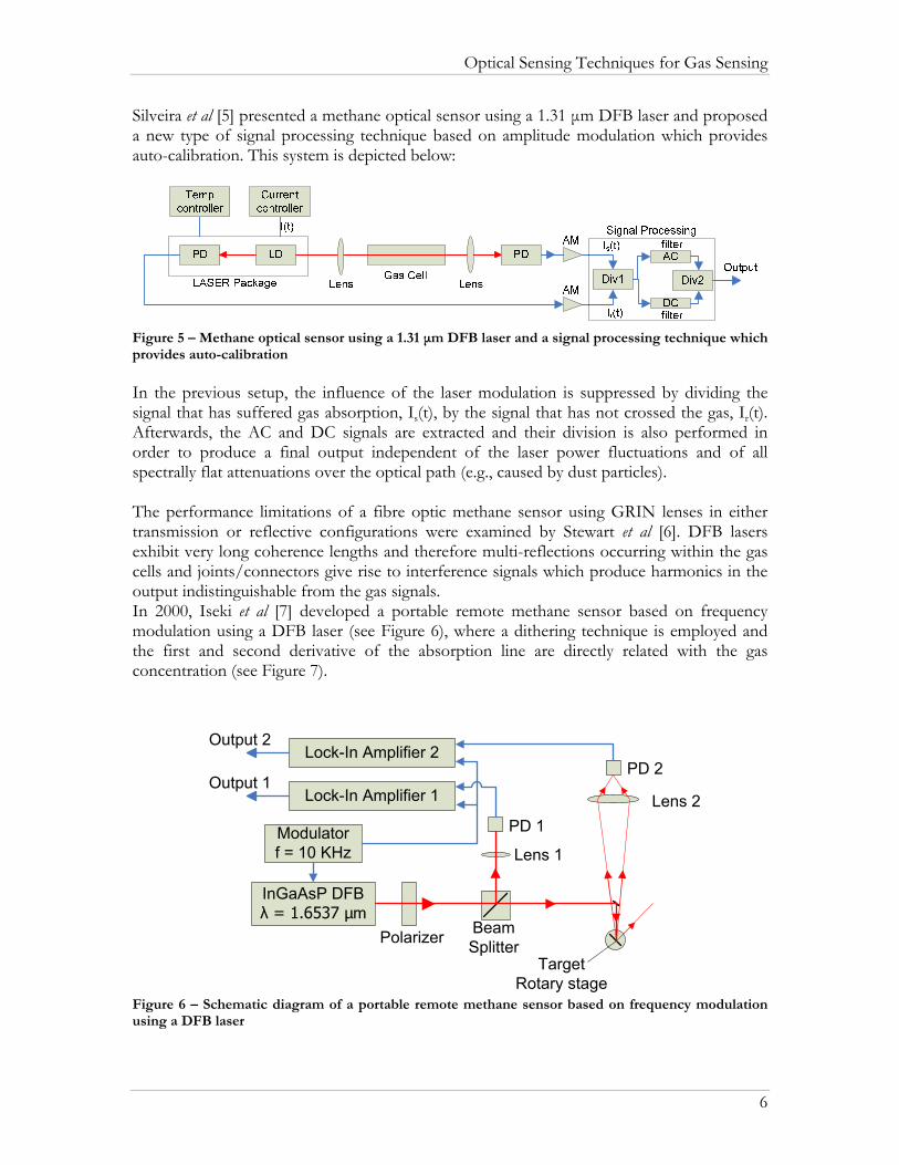
Silveira et al [5] presented a methane optical sensor using a 1.31 μm DFB laser and proposed a new type of signal processing technique based on amplitude modulation which provides auto-calibration. This system is depicted below:
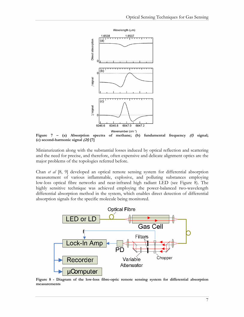
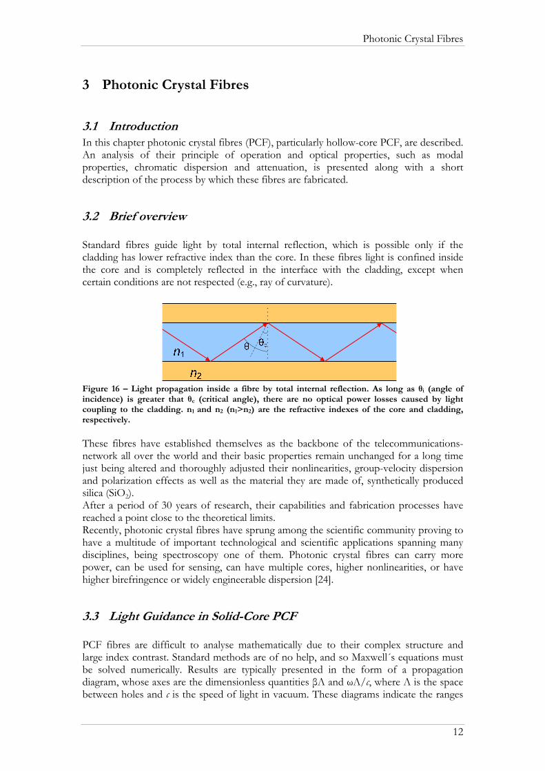
Figure 5 – Methane optical sensor using a 1.31 μm DFB laser and a signal processing technique which provides auto-calibration In the previous setup, the influence of the laser modulation is suppressed by dividing the signal that has suffered gas absorption, Is(t), by the signal that has not crossed the gas, Ir(t). Afterwards, the AC and DC signals are extracted and their division is also performed in order to produce a final output independent of the laser power fluctuations and of all spectrally flat attenuations over the optical path (e.g., caused by dust particles). The performance limitations of a fibre optic methane sensor using GRIN lenses in either transmission or reflective configurations were examined by Stewart et al [6]. DFB lasers exhibit very long coherence lengths and therefore multi-reflections occurring within the gas cells and joints/connectors give rise to interference signals which produce harmonics in the output indistinguishable from the gas signals. In 2000, Iseki et al [7] developed a portable remote methane sensor based on frequency modulation using a DFB laser (see Figure 6), where a dithering technique is employed and the first and second derivative of the absorption line are directly related with the gas concentration (see Figure 7).
Lock-In Amplifier 2
InGaAsP DFBλ = 1.6537 µm
Beam SplitterPolarizer
Lock-In Amplifier 1
Output 2
Output 1
PD 1
PD 2
Lens 2
Lens 1Modulatorf = 10 KHz
TargetRotary stage
Figure 6 – Schematic diagram of a portable remote methane sensor based on frequency modulation using a DFB laser
6
Optical Sensing Techniques for Gas Sensing
Figure 7 – (a) Absorption spectra of methane; (b) fundamental frequency (f) signal; (c) second-harmonic signal (2f) [7] Miniaturization along with the substantial losses induced by optical reflection and scattering and the need for precise, and therefore, often expensive and delicate alignment optics are the major problems of the topologies referred before. Chan et al [8, 9] developed an optical remote sensing system for differential absorption measurement of various inflammable, explosive, and polluting substances employing low-loss optical fibre networks and near-infrared high radiant LED (see Figure 8). The highly sensitive technique was achieved employing the power-balanced two-wavelength differential absorption method in the system, which enables direct detection of differential absorption signals for the specific molecule being monitored.
Figure 8 - Diagram of the low-loss fibre-optic remote sensing system for differential absorption measurements
7

Optical Sensing Techniques for Gas Sensing
In 2003, Whitenett et al [10] reported an alternative optical configuration for environmental monitoring applications, namely the utilization of cavity ring-down spectroscopy using an Erbium Doped Fibre Amplifier (EDFA). This configuration monitors the exponential decay of a light pulse inside a gas chamber that ideally exhibits very high finesse, causing therefore 1/e ring-down time to be very long and very sensitive to small changes in the cavity loss, as induced, for example, by a gas absorber in the cavity. Being an indirect measurement, it is required that the decay caused by absorption from the analyte of interest is separated from decay caused by mirror and other cavity-dependent losses.
Figure 9 – Cavity ring-down sensing system Another technique, called multipass transmission absorption spectroscopy, has been widely used and consists of a chamber with mirrors at each end filled with the sample we want to analyse. The beam is folded back and forth through the cell, creating an extended yet defined optical path length in a confined space (see Figure 10). Although it presents a high sensitivity, the slow system response to concentration fluctuations and the relatively high volume of sample required constitute its major disadvantages.
Figure 10 – Multipass transmission absorption spectroscopy scheme Photoacoustic spectroscopy [11] is another technique for detection of absorbing analytes and it relies on the photoacoustic effect. In this technique, the sample gas is confined in a chamber, where modulated (e.g., chopped) radiation enters via a transparent window and is absorbed by active molecular species, for the wavelength considered. The temperature of the gas thereby increases, leading to a periodic expansion and contraction of the gas volume synchronous with the modulation frequency of the radiation. This, consequently, produces a pressure wave that can be detected by simple microphones as depicted in the figure below.
Figure 11 – Photoacoustic spectroscopy diagram
8

Optical Sensing Techniques for Gas Sensing
Even being highly sensitive, requiring reduced volumes of gas and avoiding the need for optical detection this technique has some drawbacks, being its sensitivity to vibrational noise the most important one. Other approaches have also been implemented, exploring different types of fibres (e.g., D-fibre) and effects, such as evanescent wave absorption [12]. Their major obstacles, namely low sensitivity for short interaction lengths, spurious interference effects and degradation through surface contamination, were analysed [13] and it was determined that the sensitivity of a D-fibre methane gas sensor could be improved by overcoating the flat surface of the fibre with a high index layer, reaching a detection limit lower than 5 ppm [14]. More recently, several authors proposed new methods for gas detection. Benounis et al [15] demonstrated a new evanescent fibre sensor based on cryptophane molecules deposited on a PCS (polycarbosilane) fibre. Roy et al [16] demonstrated a methane sensor based on the utilization of carbon tubes and nanofibres deposited by an electro-deposition technique.
2.3 Photonic crystal fibers in gas sensing technology The holes in microstructured fibres open up new opportunities for exploiting the interaction of light with gases or liquids through the evanescent field effect. A new range of applications for these fibres has already been brought into light, being gas sensing one of them. New designs have also been proposed and improved, including detailed simulations of their guidance properties [17, 18].
Figure 12 – Two solid-core holey optical fibres [17]
One class of microstructured fibres is the air-guiding photonic band gap fibres. These fibres confine light within the air core by a two-dimensional photonic bandgap formed by the periodic structure of the cladding, which permits transmission over a limited wavelength range [19]. A novel fibre design (see Figure 13), proposed by Ritari et al [20], was used to demonstrate a high sensitivity gas sensing system.
Figure 13 – Microscope images of air-guiding photonic bandgap fibres proposed for gas sensing [19]
9

Optical Sensing Techniques for Gas Sensing
In 2007, two methane detection systems based on the use of Photonic Bandgap Fibres were presented [21, 22]. These systems explored the long interaction path-lengths achievable with this type of fibres and enabled the detection of reduced concentrations of CH4 in air. The presented detection limits were 0.1% of methane in air, operating at 1331.55 nm [21], and 10 ppmv, operating at ~1645 nm and employing a multiline fit algorithm due to the collisional broadening caused by the experimental setup that turned impossible to identify individual transitions in the referred absorption band [22]. The following configuration was used to perform the experiments:
Figure 14 – Experimental setup used to perform experiments [21] It should be noticed that it is the gap between the HC-PBF and the SMF that allows the gas diffusion into the hollow-core, with the SMF being angle cleaved to avoid Fresnel reflections that could interfere in the measurements. Water absorption can become a problem for the system operating in the 1330 nm region [23, 24]. Power fluctuations from the light source, power losses induced by misalignment or fibre bending and diffusion time of gas inside the fibre constitute drawbacks to both systems. Further research and more sensitive techniques, such as modulation schemes, could led to the achievement of higher sensitivities and lower response time sensors.
2.4 Pellistors in gas sensing technology Although pellistors are not an optical gas sensing method they are the most widely used gas sensing method and therefore a brief description of their principle of operation will be presented here. Catalytic combustion has been the most widely used method of detecting flammable gases in industry since the invention of the catalytic pelletized resistor (or pellistor) in the mid 1960's. A pellistor consists of a very fine coil of platinum wire, embedded within a ceramic pellet. On the surface of that pellet is a layer of a high surface area noble metal, which, when hot, acts as a catalyst to promote exothermic oxidation of flammable gases. In operation, the pellet and so the catalyst layer is heated by passing a current through the underlying coil. In the presence of a flammable gas or vapour, the hot catalyst allows oxidation to occur in a similar chemical reaction to combustion. Just as in combustion, the reaction releases heat, which causes the temperature of the catalyst together with its underlying pellet and coil to rise. This rise in temperature results in a change of the electrical resistance of the coil, and it is this change in electrical resistance that constitutes the signal from the sensor. Pellistors are always manufactured in pairs, the active catalysed element being supplied with an electrically matched element which contains no catalyst and is treated to ensure
10

Optical Sensing Techniques for Gas Sensing
no flammable gas will oxidise on its surface. This "compensator" element is used as a reference resistance to which the sensor's signal is compared, to remove the effects of environmental factors other than the presence of a flammable gas.
Figure 15 – Pellistor drive/measurement circuit These thermocatalytic devices have, however, their limitations and in particular they are susceptible to surface poisoning which raises the need for scheduled replacement and consequent increase of cost. The amount of needed power constitutes a limitation in terms of security, because of the inherent risk of explosion and in terms of distance between the sensor and power source. They are also non-selective since any gas whose ignition is catalysed will be detected.
2.5 Summary Several architectures have already been implemented in order to effectively detect gases in the atmosphere by optical absorption spectroscopy, some of them reaching good sensitivity levels with fast response times. However, most of these techniques imply the need for precise alignments and optical power losses constitute another problem in their implementation, prohibiting its usage over remote/long distances. Photoacoustic spectroscopy is another method that attempts to detect gases with a relatively simple setup which enables the achievement of fairly good results being the influence of other sources of vibrational noise its major limitation. Microstructured optical fibres, as well as standard fibres, enable the implementation of remote detection systems since light is guided along their structure consequently avoiding possible sources of contamination or loss. More particularly, hollow-core photonic bandgap fibres, being the main subject of the work here presented, represent a solution where large direct interaction lengths between light and gas can be attained, empowering their usage and the implementation of reduced dimensions gas sensing systems. Comparing pellistors with optical detection, the former detects the presence of gas only at specific points, whereas the latter detects an average concentration over the interrogated path length being much more gas selective. The amount of power and the risk of explosion inherent to the principle of operation of pellistors are two problems that optical detection methods do not give rise to.
11
Photonic Crystal Fibres
3 Photonic Crystal Fibres
3.1 Introduction In this chapter photonic crystal fibres (PCF), particularly hollow-core PCF, are described. An analysis of their principle of operation and optical properties, such as modal properties, chromatic dispersion and attenuation, is presented along with a short description of the process by which these fibres are fabricated.
3.2 Brief overview Standard fibres guide light by total internal reflection, which is possible only if the cladding has lower refractive index than the core. In these fibres light is confined inside the core and is completely reflected in the interface with the cladding, except when certain conditions are not respected (e.g., ray of curvature).
Figure 16 – Light propagation inside a fibre by total internal reflection. As long as θi (angle of incidence) is greater that θc (critical angle), there are no optical power losses caused by light coupling to the cladding. n1 and n2 (n1>n2) are the refractive indexes of the core and cladding, respectively. These fibres have established themselves as the backbone of the telecommunications-network all over the world and their basic properties remain unchanged for a long time just being altered and thoroughly adjusted their nonlinearities, group-velocity dispersion and polarization effects as well as the material they are made of, synthetically produced silica (SiO2). After a period of 30 years of research, their capabilities and fabrication processes have reached a point close to the theoretical limits. Recently, photonic crystal fibres have sprung among the scientific community proving to have a multitude of important technological and scientific applications spanning many disciplines, being spectroscopy one of them. Photonic crystal fibres can carry more power, can be used for sensing, can have multiple cores, higher nonlinearities, or have higher birefringence or widely engineerable dispersion [24].
3.3 Light Guidance in Solid-Core PCF PCF fibres are difficult to analyse mathematically due to their complex structure and large index contrast. Standard methods are of no help, and so Maxwell´s equations must be solved numerically. Results are typically presented in the form of a propagation diagram, whose axes are the dimensionless quantities βΛ and ωΛ/c, where Λ is the space between holes and c is the speed of light in vacuum. These diagrams indicate the ranges
12

Photonic Crystal Fibres
of frequency and axial wave vector component β where light is evanescent (unable to propagate). At fixed optical frequency, the maximum possible value of β is set by kn =ωn/c, where n is the refractive index of the region under consideration and k is the free-space propagation constant. For β < kn, light is free to propagate; for β > kn, it is evanescent. For conventional fibre (core and cladding refractive indices nco and ncl, respectively), guided modes appear when light is free to propagate in the doped core but is evanescent in the cladding (Figure 17-A). The same diagram for PCF is sometimes known as a band-edge or “finger” plot. In a triangular lattice of circular air holes with an air-filling fraction of 45%, light is evanescent in the black regions of Figure 17-B. Full two-dimensional photonic band gaps exist within the black finger-shaped regions, some of which extend into β < k where light is free to propagate in vacuum. This result indicates that hollow-core guidance is indeed possible in the silica-air system.
Figure 17 – Propagation diagrams for (A) a conventional single-mode fibre with a Ge-doped silica core and a pure silica cladding and for (B) a solid-core PCF. [24] From the analysis of Figure 17-A we can state that guided modes form at points like R, where light is free to travel in the core but unable to penetrate the cladding (total internal reflection). The narrow red strip is where the whole of optical telecommunications operates. In Figure 17-B it is represented the propagation diagram for a triangular lattice of air channels in silica glass with 45% air-filling fraction, with four distinct regions. In region (1), light is free to propagate in every region of the fibre [air, photonic crystal (PC), and silica]. In region (2), propagation is turned off in the air, and, in (3) it is turned off in the air and the PC. In (4), light is evanescent in every region. The black fingers represent the regions where full two-dimensional photonic band gaps exist. Guided modes of a solid-core PCF (see schematic in the top left-hand corner of Figure 17-B) form at points such as Q, where light is free to travel in the core but unable to penetrate the PC. At point P, light is free to propagate in air but blocked from penetrating the cladding by the PBG; these are the conditions required for a hollow-core mode. It is mind-boggling that the entire optical telecommunications revolution happened within the narrow red strip knclΛ<βΛ<kncoΛ of Figure 17-A. The rich variety of new features on the diagram for PCF explains in part why microstructuring extends the possibilities of fibres so greatly.[24]
13

Photonic Crystal Fibres
14
3.4 Light Guidance in Hollow-Core PCF The first successful hollow-core PCF, was reported in 1999 and consisted in a triangular lattice of holes from which were removed seven capillaries to form an hollow-core, large enough to improve the capability of finding a guided mode [19]. For the existence of a vacuum-guided mode the following relation must be observed, β/k<1, so the relevant operation region in Figure 17-B is to the left of the vacuum line, inside one of the fingers. This will ensure light will be trapped inside the core and unable to propagate in the cladding. At the moment, there are two types of hollow-core PCF available, the 7-cell and the 19-cell PCF. In the case of the 7-cell PCF the core is formed by removing 7 capillaries from the cladding, while in the 19-cell case are obviously removed 19 capillaries.
Figure 18 – Hollow-core PCF from BlazePhotonics; a) 7-cell PCF (HC-1550-02); b) 19-cell PCF (HC19-1550-01). [25]
The 7-cell PCF exhibits a larger and continuous operating bandwith and a smaller number of core modes and parasitic surface modes. For the 19-cell PCF case, there is a larger mode field diameter as well as a lower M2 of fundamental mode, it is more gaussian-like, resulting in increased coupling efficiency to high-mode quality lasers and conventional fibres. The 19-cell PCF also present lower attenuation, dispersion and dispersion slope. Their nonlinearities are also lower contrasting with the higher breakdown power threshold. [26]
Figure 19 – Transmission spectra for a 7-cell (HC-1550) and a 19-cell core fiber (HC19-1550), both designed for operation at 1550 nm. [26]
a) b)

Photonic Crystal Fibres
Within these types of fibres, light is not guided by total internal reflection but by light confinement in a waveguide, similar in principle to those for microwave propagation. Imagine a multi-layer mirror that for certain angles and optical wavelengths coherently adds up reflections from each layer, transforming the cladding into an almost perfect 2-D mirror which maintains light confined in the core of the fibre. This virtually loss-free mirror is called a photonic band gap (PBG), and is created by a periodic wavelength-scale lattice of microscopic holes in the cladding glass – a photonic crystal – that inherently have certain angles and colours (“stop bands”) where light is strongly reflected. This is how butterfly wings, peacock feathers and holograms such as those found in credit cards exhibit such beautiful effects and colours.
Figure 20 – Photonic crystal microstructure found in the wings of Cyanophrys remus butterflies
In a hollow-core PCF, the core is created by introducing a defect in the PBG structure (e.g. an extra air hole), thereby creating an area where the light can propagate. As the light can only propagate at the defect region, a low index guiding core has been created.
Figure 21 – Optical micrograph exhibiting the near-field of a red mode in a hollow-core PCF, with white light being injected into the core. [26]
3.5 PCF Fabrication In the beginning, PCF fabrication revealed to be a problem in the way that nothing similar has been made before, so a fabrication method had to be idealized. While conventional single-mode optical fibres’ core and cladding materials have similar refractive indexes (typically differing by around a percent), photonic crystal fibres require a far higher refractive index contrast, differing by perhaps 50-100%.
15
Photonic Crystal Fibres
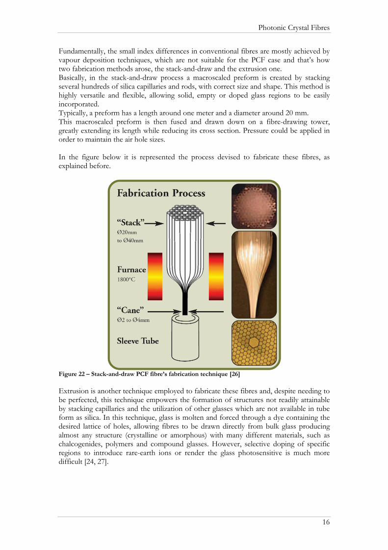
Fundamentally, the small index differences in conventional fibres are mostly achieved by vapour deposition techniques, which are not suitable for the PCF case and that’s how two fabrication methods arose, the stack-and-draw and the extrusion one. Basically, in the stack-and-draw process a macroscaled preform is created by stacking several hundreds of silica capillaries and rods, with correct size and shape. This method is highly versatile and flexible, allowing solid, empty or doped glass regions to be easily incorporated. Typically, a preform has a length around one meter and a diameter around 20 mm. This macroscaled preform is then fused and drawn down on a fibre-drawing tower, greatly extending its length while reducing its cross section. Pressure could be applied in order to maintain the air hole sizes. In the figure below it is represented the process devised to fabricate these fibres, as explained before.
Figure 22 – Stack-and-draw PCF fibre’s fabrication technique [26] Extrusion is another technique employed to fabricate these fibres and, despite needing to be perfected, this technique empowers the formation of structures not readily attainable by stacking capillaries and the utilization of other glasses which are not available in tube form as silica. In this technique, glass is molten and forced through a dye containing the desired lattice of holes, allowing fibres to be drawn directly from bulk glass producing almost any structure (crystalline or amorphous) with many different materials, such as chalcogenides, polymers and compound glasses. However, selective doping of specific regions to introduce rare-earth ions or render the glass photosensitive is much more difficult [24, 27].
16

Photonic Crystal Fibres
3.6 Optical Properties
3.6.1 Modal Properties Similar to conventional optical fibres, hollow-core PCF exhibit an intensity profile closely matching a Gaussian distribution, being able to achieve, in the case of the 19-cell PCF operating at 1550 nm, a shape overlap >97% with the fundamental mode of an all-solid step index fibre, thus facilitating coupling to high mode quality lasers or conventional fibres.
Figure 23 – Typical near field intensity distribution for a 19-cell PCF. [25] Even though hollow-core PCF are intended to be used like other single mode fibres, it must be taken into account their higher order core modes and eventual core-cladding interface modes, when designing input and output coupling optics, despite their rapid decay and higher losses compared to those of the fundamental mode. [26]
3.6.2 Chromatic Dispersion While in conventional fibres material is the main responsible for dispersion, in hollow-core PCF Group-Velocity Dispersion (GVD) is dominated by waveguide dispersion. In the following figure, it is represented the typical attenuation and chromatic dispersion spectrum of a HC19-1550-01:
Figure 24 - Typical attenuation and chromatic dispersion spectrum of a HC19-1550-01 [25]
17
Photonic Crystal Fibres
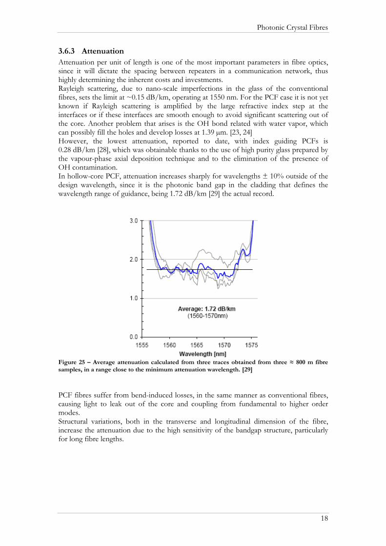
3.6.3 Attenuation Attenuation per unit of length is one of the most important parameters in fibre optics, since it will dictate the spacing between repeaters in a communication network, thus highly determining the inherent costs and investments. Rayleigh scattering, due to nano-scale imperfections in the glass of the conventional fibres, sets the limit at ~0.15 dB/km, operating at 1550 nm. For the PCF case it is not yet known if Rayleigh scattering is amplified by the large refractive index step at the interfaces or if these interfaces are smooth enough to avoid significant scattering out of the core. Another problem that arises is the OH bond related with water vapor, which can possibly fill the holes and develop losses at 1.39 µm. [23, 24] However, the lowest attenuation, reported to date, with index guiding PCFs is 0.28 dB/km [28], which was obtainable thanks to the use of high purity glass prepared by the vapour-phase axial deposition technique and to the elimination of the presence of OH contamination. In hollow-core PCF, attenuation increases sharply for wavelengths ± 10% outside of the design wavelength, since it is the photonic band gap in the cladding that defines the wavelength range of guidance, being 1.72 dB/km [29] the actual record.
Figure 25 – Average attenuation calculated from three traces obtained from three ≈ 800 m fibre samples, in a range close to the minimum attenuation wavelength. [29] PCF fibres suffer from bend-induced losses, in the same manner as conventional fibres, causing light to leak out of the core and coupling from fundamental to higher order modes. Structural variations, both in the transverse and longitudinal dimension of the fibre, increase the attenuation due to the high sensitivity of the bandgap structure, particularly for long fibre lengths.
18

Photonic Crystal Fibres
19
3.7 Summary Photonic crystals are periodically structured dielectric media, generally possessing ranges of frequency in which light cannot propagate through the structure (photonic bandgap). This periodicity, whose lengthscale is proportional to the wavelength of light in the band gap, is the electromagnetic analogue of a crystalline atomic lattice and is typically provided by air voids running along the length of the fibre. Photonic bandgap fibres, being made of a single material, do not exhibit boundaries between two types of glass and, consequently, no different thermal expansion coefficients, which, when present, can lead to optical losses. Regarding the fact that in hollow-core PCF as much as 99% of the optical power can travel in air and not in the glass, we can say that they are less prone to losses than conventional fibres. From an attenuation point of view, photonic crystal fibres are reaching a stage where we can start to guess conventional fibres being outdone in a not so far future.

Wavelength Modulation Spectroscopy
4 Wavelength Modulation Spectroscopy
4.1 Introduction This chapter describes the signal processing technique chosen in the scope of this project, namely Wavelength Modulation Spectroscopy, along with a mathematical analysis of its principle and corresponding simulation results.
4.2 Definition The simplest approach for doing absorption spectroscopy, using hollow-core PCF, would be to use an interrogation system consisting of a source, a HC-PCF-based gas cell and a photo-detector, as shown in Figure 26. Although this is a simple system, it’s not robust and any losses caused by fibre bending; misalignment or other causes would not be discerned from variations in the gas concentration. Therefore, there is the need to implement another detection technique and that’s where Wavelength Modulation Spectroscopy (WMS) arises.
Figure 26 - The simplest sensor configuration for measuring changes in optical transmitted power WMS is a rather straightforward technique that enables us to improve the detection accuracy. For this method, the source should have a linewidth significantly smaller than the absorption line to be monitored. In this technique, the source’s wavelength is slowly modulated, sweeping the entire absorption peak, and a higher frequency signal (dithering) is superimposed on this signal. As the emission source wavelength slowly scans through the gas absorption line, the wavelength modulation becomes an amplitude modulation, presenting its highest amplitude as it passes in the highest slope points of the absorption peak (see below).
Figure 27 – Wavelength modulation converted to amplitude modulation in Wavelength Modulation Spectroscopy This method shifts the detection bandwidth to higher frequencies where laser intensity noise is reduced towards the shot noise limit and consequently the signal-to-noise ratio is highly increased. This concept is similar to that of data encoding in the side bands of a radio transmission carrier wave. Figure 28 shows the spectral output of a radio frequency modulated laser, where can be seen the carrier frequency ωc and the side band frequencies ωc±Ω. So, when the laser slowly scans through the absorption line, the amount of light absorbed, which by the Lambert-Beer Law is proportional to the gas concentration, is “written” into the side bands. Schematically, this is represented in Figure 28 c) as a decrease in the amplitude of the side bands.
20

Wavelength Modulation Spectroscopy
Figure 28 – Spectral output of a laser beam: a) unmodulated; b) modulated with no absorption; c) modulated with absorption. The absorption information can be retrieved by means of a lock-in amplifier, where a voltage output proportional to gas concentration can be generated (Figure 29).
-0,05
0,00
0,05
0,10
-0,2
0,0
0,2
0,4
-6
-4
-2
0
Wavelength
Wavelength
Wavelength
Am
plitu
de (V
)
2nd harmonic
Am
plitu
de (V
)
1st harmonic
λcentral
1530,35 nm
Nor
mal
ized
Pow
er (d
B) Acetylene gas cell absorption peak
Figure 29 – WMS output obtained with a lock-in amplifier, locked at dithering frequency (experimental data obtained with the implemented setup).
Paying attention to Figure 29, in red we can clearly see that this response is the first derivative of the gas absorption line and that it equals zero when the source wavelength is centred in the absorption peak. Subsequently, the lock-in amplifier output for the second harmonic is the derivative trace of the output at the dithering frequency and is maximum at this point (blue signal). By disabling the slow modulation and stabilizing the source emission wavelength at the absorption peak, the dithering gives rise to a transmitted signal with an amplitude that depends on the gas concentration and which frequency is twice the dithering one (see Figure 30).
21

Wavelength Modulation Spectroscopy
22
Figure 30 - Frequency duplication phenomenon, resulting from dithering at the absorption peak.
This way of detection thus converts a frequency modulation into an amplitude modulation, which can easily be detected by a simple photodetector. The measured signal will contain both an AC and a DC component. Fluctuations of the optical power (from the source, fibre bends, …) will commonly modify the AC and DC components of the signal, so the computed signal given by the ratio of the AC component and the DC component remains fairly unaltered, being only affected by the gas concentration. This insensitivity to power fluctuations is one of the main advantages of the WMS-method.
4.3 Mathematical analysis In order to further evaluate the feasibility of the WMS-method as an applicable solution for the intended purpose, the simple system depicted in Figure 31 was considered and the following mathematical analysis was carried out.
Figure 31 – Simple configuration to directly quantify gas absorption The function that describes the spectral distribution of optical power emitted by the DFB can be described by a Gaussian, that is:
( )⎥⎥⎦
⎤
⎢⎢⎣
⎡⎟⎟⎠
⎞⎜⎜⎝
⎛Δ
−−
Δ=
2
2ln4exp2ln2
DFB
o
DFB
TPPλ
λλπλ
λ , 4.1
being the total optical power, TP DFBλΔ the full width at half maximum and oλ the emission central wavelength. Considering just one absorption peak, the gas cell transfer function can be approached by an inverted Gaussian, i.e.,
( ) ⎟⎟
⎠
⎞
⎜⎜
⎝
⎛
⎥⎥⎦
⎤
⎢⎢⎣
⎡⎟⎟⎠
⎞⎜⎜⎝
⎛Δ−
−−=2
2ln4exp1GC
GCo ATT
λλλλ , 4.2
Amplitude modulated signal (2ω)
Amplitude
Dithering at ω
Absorption peak
ν
Wavelength Modulation Spectroscopy
where represents the maximum transmissivity (including insertion losses), oT A is a parameter that describes the absorption of the referred line, GCλΔ its full width at half maximum and GCλ its wavelength. The detector’s received optical power can, then, be calculated by the usual means:
( ) ( )∫∞
=0
λλλβ dTPPOUT . 4.3
In the previous expression, β is a factor that represents the optical power losses occurred in the optical path to the detector, which can vary with time. Generally, the spectral width of the absorption peak, GCλΔ , is much higher than the spectral width of the laser mode, DFBλΔ . That way, we can consider that the spectral response of the absorption peak does not vary in the wavelength interval defined by the laser’s mode width, being the cell’s transfer function in that interval defined by ( )oT λ . The previous integral is, then, simplified to:
⎥⎥
⎦
⎤
⎢⎢
⎣
⎡
⎥⎥⎦
⎤
⎢⎢⎣
⎡⎟⎟⎠
⎞⎜⎜⎝
⎛Δ−
−−≈2
2ln4exp1GC
GCooTOUT ATPP
λλλβ . 4.4
Let’s now consider that the DFB injection current is modulated with a sinusoidal signal of small amplitude. In this case, the wavelength of the central emitted mode becomes time-dependent:
( ) tt oo ωδλλλ sen+= . 4.5
In the previous expression, δλ is the modulation amplitude of the central wavelength of the mode emitted by the DFB, oλ is the average central laser’s mode wavelength and ω is the angular frequency associated with the “dither” signal. Using this expression, the signal in the detector can be written as
( )⎥⎥
⎦
⎤
⎢⎢
⎣
⎡
⎥⎥⎦
⎤
⎢⎢⎣
⎡⎟⎟⎠
⎞⎜⎜⎝
⎛Δ
+Δ−−≈+Δ
2sen2ln4exp1sen
GCoTOUT
tATPtPλ
ωδλλβωδλλ , 4.6
where GCo λλλ −=Δ . As the modulation amplitude is generally small, a Taylor’s series can be used to approximately describe the components at DC, at ω and at ω2 :
( )⎥⎥
⎦
⎤
⎢⎢
⎣
⎡
⎥⎥⎦
⎤
⎢⎢⎣
⎡⎟⎟⎠
⎞⎜⎜⎝
⎛
ΔΔ
−−≈+Δ2
2ln4exp1senGC
oTDC
OUT ATPtPλλβωδλλ , 4.7
( ) tATPtPGCGC
oTOUT ωλλδλλ
λβωδλλω sen2ln4exp2ln2sen
2
2 ⎥⎥⎦
⎤
⎢⎢⎣
⎡⎟⎟⎠
⎞⎜⎜⎝
⎛
ΔΔ
−ΔΔ
≈+Δ , 4.8
23

Wavelength Modulation Spectroscopy
( ) ( )tATPtPGCGCGC
oTOUT ωλλλ
λδλ
λβωδλλω 2cos2ln4exp
412ln22lnsen
22
22
22
⎥⎥⎦
⎤
⎢⎢⎣
⎡⎟⎟⎠
⎞⎜⎜⎝
⎛ΔΔ
−⎟⎟⎠
⎞⎜⎜⎝
⎛+Δ
Δ−
Δ−≈+Δ .
4.9
When a perfect tune exists between the laser’s emission wavelength and the point of maximum absorption for the selected line, i.e., 0=Δλ , we have
[ ]ATPP oTDC
OUT −≈ 1β , 4.10
( ) 0≈ωOUTPAmpl , 4.11
( )2
2
42ln
⎟⎟⎠
⎞⎜⎜⎝
⎛Δ
≈GC
oTOUT ATPPAmplλδλβω . 4.12
As expected, the amplitude is null at the fundamental frequency. For the amplitude at double frequency it is proportional to A but also shows losses dependency. This drawback can be overcome dividing the ω2 component’s amplitude by the DC component, obtaining a signal proportional to
2
142ln
⎟⎟⎠
⎞⎜⎜⎝
⎛Δ−
=GC
OUT AAkS
λδλ , 4.13
where k represents the several optical/electrical transduction and amplification coefficients involved. The output signal is, then, losses-independent, of the optical emitted power and of the gas-cell’s insertion losses. Using Beer-Lambert’s law the parameter can be related to concentration: A
( )CLII INOUT α−= exp , 4.14
where α represents the absorption constant of the gas in the cell, in cm-1atm-1, the concentration and the interaction length between the radiation and the gas (cell length), in cm. If we define
CL
( )CLI
ITIN
OUT α−== exp , 4.15
then is simply given by A
TA −= 1 , 4.16
and the expression for becomes: OUTS
( )[ ]1exp42ln
2
−⎟⎟⎠
⎞⎜⎜⎝
⎛Δ
= CLkSGC
OUT αλδλ . 4.17
24

Wavelength Modulation Spectroscopy
The output signal then exhibits a dependency approximately linear with concentration, since the aimed values are generally low. For reference, the components at DC and at ω2 can also be expressed as a function of the concentration:
( )CLTPP oTDC
OUT αβ −≈ exp , 4.18
( ) ([ ]CLTPPAmplGC
oTOUT αλδλβω −−⎟⎟
⎠
⎞⎜⎜⎝
⎛Δ
≈ exp142ln
22 ) . [30] 4.19
4.4 Simulation results In order to evaluate the previously presented analysis, some simulations were performed and the results are now presented. The values used for the different variables are presented below:
18.0 −= cmα WPT
3105 −×= 9.0=oT
pm150=δλ pmGC 300=Δλ
1000=k For an interaction length of 3 cm, we varied β from 0.3 to 0.9 with increments of 0.3.
and were plotted as well as their ratio, DCOUTA ω2
OUTA DCOUT
OUTOut A
ASϖ2
= .
The obtained results are displayed, below:
1.μ 10-9 11000
H%L Concentration
0.0015
0.0020
0.0025
0.0030
0.0035
0.0040
HVL AOutDC
L = 3 cm
b=0.9
b=0.6
b=0.3
Figure 32 – Simulation result for (L=3 cm) DC
OUTA
25

Wavelength Modulation Spectroscopy
1.μ 10-9 11000
H%L Concentration
1. μ10-7
2. μ10-7
3. μ10-7
4. μ10-7
HVL AOut2w
L = 3 cm
b=0.9
b=0.6
b=0.3
Figure 33 - Simulation result for (L=3 cm)
ω2OUTA
1.μ 10-9 11000
H%L Concentration
0.02
0.04
0.06
0.08
0.10
SOut
L = 3 cm
b=0.9
b=0.6
b=0.3
Figure 34 - Simulation result for DCOUT
OUT
AA ϖ2
(L=3 cm)
For an interaction length of 5 cm the same procedure was repeated and the results are as follows:
1.μ 10-9 11000
H%L Concentration
0.0015
0.0020
0.0025
0.0030
0.0035
0.0040
HVL AOutDC
L = 5 cm
b=0.9
b=0.6
b=0.3
Figure 35 - Simulation result for (L=5 cm) DC
OUTA
26
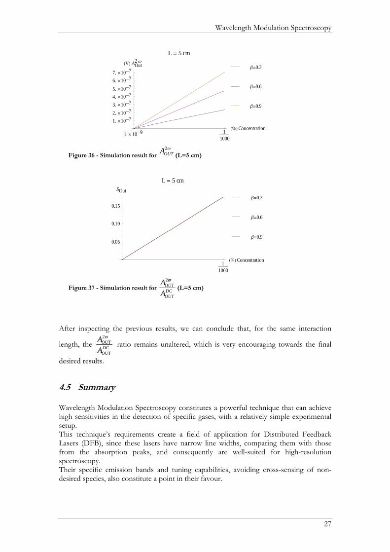
Wavelength Modulation Spectroscopy
1.μ 10-9 11000
H%L Concentration1. μ10-72. μ10-73. μ10-74. μ10-75. μ10-76. μ10-77. μ10-7
HVL AOut2w
L = 5 cm
b=0.9
b=0.6
b=0.3
Figure 36 - Simulation result for (L=5 cm)
ω2OUTA
11000
H%L Concentration
0.05
0.10
0.15
SOut
L = 5 cm
b=0.9
b=0.6
b=0.3
Figure 37 - Simulation result for DCOUT
OUT
AA ϖ2
(L=5 cm)
After inspecting the previous results, we can conclude that, for the same interaction
length, the DCOUT
OUT
AA ϖ2
ratio remains unaltered, which is very encouraging towards the final
desired results.
4.5 Summary Wavelength Modulation Spectroscopy constitutes a powerful technique that can achieve high sensitivities in the detection of specific gases, with a relatively simple experimental setup. This technique’s requirements create a field of application for Distributed Feedback Lasers (DFB), since these lasers have narrow line widths, comparing them with those from the absorption peaks, and consequently are well-suited for high-resolution spectroscopy. Their specific emission bands and tuning capabilities, avoiding cross-sensing of non-desired species, also constitute a point in their favour.
27

Wavelength Modulation Spectroscopy
The effects caused from several possible sources of losses, such as fibre bending,
coupling losses, misalignment, etc., can be omitted by the DCOUT
OUT
AA ϖ2
ratio, which outputs a
signal that only portrays gas concentration. The simulation’s results, supported by the presented mathematical model analysis, strongly encourage the implementation of this technique towards our final goal.
28
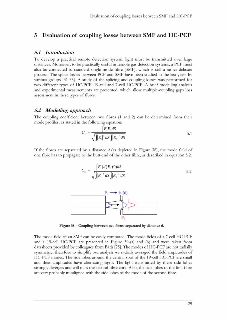
Evaluation of coupling losses between SMF and HC-PCF
29
5 Evaluation of coupling losses between SMF and HC-PCF
5.1 Introduction To develop a practical remote detection system, light must be transmitted over large distances. Moreover, to be practically useful in remote gas detection systems, a PCF must also be connected to standard single mode fibre (SMF), which is still a rather delicate process. The splice losses between PCF and SMF have been studied in the last years by various groups [31-35]. A study of the splicing and coupling losses was performed for two different types of HC-PCF: 19-cell and 7-cell HC-PCF. A brief modelling analysis and experimental measurements are presented, which allow multiple-coupling gaps loss assessment in these types of fibres.
5.2 Modelling approach The coupling coefficient between two fibres (1 and 2) can be determined from their mode profiles, as stated in the following equation:
*1 2
12 2 2
1 2
E E dSC
E dS E dS= ∫
∫ ∫ 5.1
If the fibres are separated by a distance d (as depicted in Figure 38), the mode field of one fibre has to propagate to the butt-end of the other fibre, as described in equation 5.2.
*1 2
12 2 2
1 2
( ) (0)E d E dSC
E dS E dS= ∫
∫ ∫ 5.2
Figure 38 – Coupling between two fibres separated by distance d.
The mode field of an SMF can be easily computed. The mode fields of a 7-cell HC-PCF and a 19-cell HC-PCF are presented in Figure 39-(a) and (b) and were taken from datasheets provided by colleagues from Bath [25]. The modes of HC-PCF are not radially symmetric, therefore to simplify our analysis we radially averaged the field amplitudes of HC-PCF modes. The side lobes around the central spot of the 19-cell HC-PCF are small and their amplitudes have alternating signs. The light transmitted by these side lobes strongly diverges and will miss the second fibre core. Also, the side lobes of the first fibre are very probably misaligned with the side lobes of the mode of the second fibre.
E1 E1(d)
E2

Evaluation of coupling losses between SMF and HC-PCF
30
Figure 39 – (a) Mode of a 7-cell HC-PCF; (b) Mode of a 19-cell HC-PCF; (c) Radially averaged mode of a 7-cell HC-PCF; (d) Radially averaged mode of a 19-cell HC-PCF.
Our estimation for the portion of light propagating in the side holes of a 19-cell HC-PCF is 1.8%. Therefore, we assume that the light in the side lobes of the 19-cell HC-PCF is effectively lost and not coupled to the other fibre. The radial average mode profiles of the 7-cell HC-PCF and the 19-cell HC-PCF are shown in Figure 39-(c) and (d), and also in Figure 40.
0 2 4 6 8 10 12 14 16
0,0
0,2
0,4
0,6
0,8
1,0
Nor
mal
ized
mod
e am
plitu
de
Distance from core centre (μm)
19 cell
7 cell
SMF
Figure 40 – Radial average of mode profiles for SMF, 7-cell HC-PCF, and 19-cell HC-PCF.
We used the mode profile of the left fibre of Figure 38 (assuming it is centre-symmetrical) and simulated how it propagates in the free space between the two fibres by decomposing the beam into space Fourier components. The coupling coefficients for SMF → 7-cell HC-PCF, SMF → 19-cell HC-PCF, and 19-cell HC-PCF → 19-cell HC-PCF, were then calculated according to equation 5.2. The decomposition of mode profiles of the SMF, the 7-cell HC-PCF, and the 19-cell HC-PCF showed that more than 95% of the beam is in the zero-order Gaussian beam. The major difference between the fibres under analysis is then in the mode field diameter. Therefore, it is a good approximation to consider that the beams have Gaussian profiles. The coupling coefficient between two Gaussian beams radiated from two fibres at distance d can be found from equation 5.2 and is presented as follows:
(a) (b)
(c) (d)
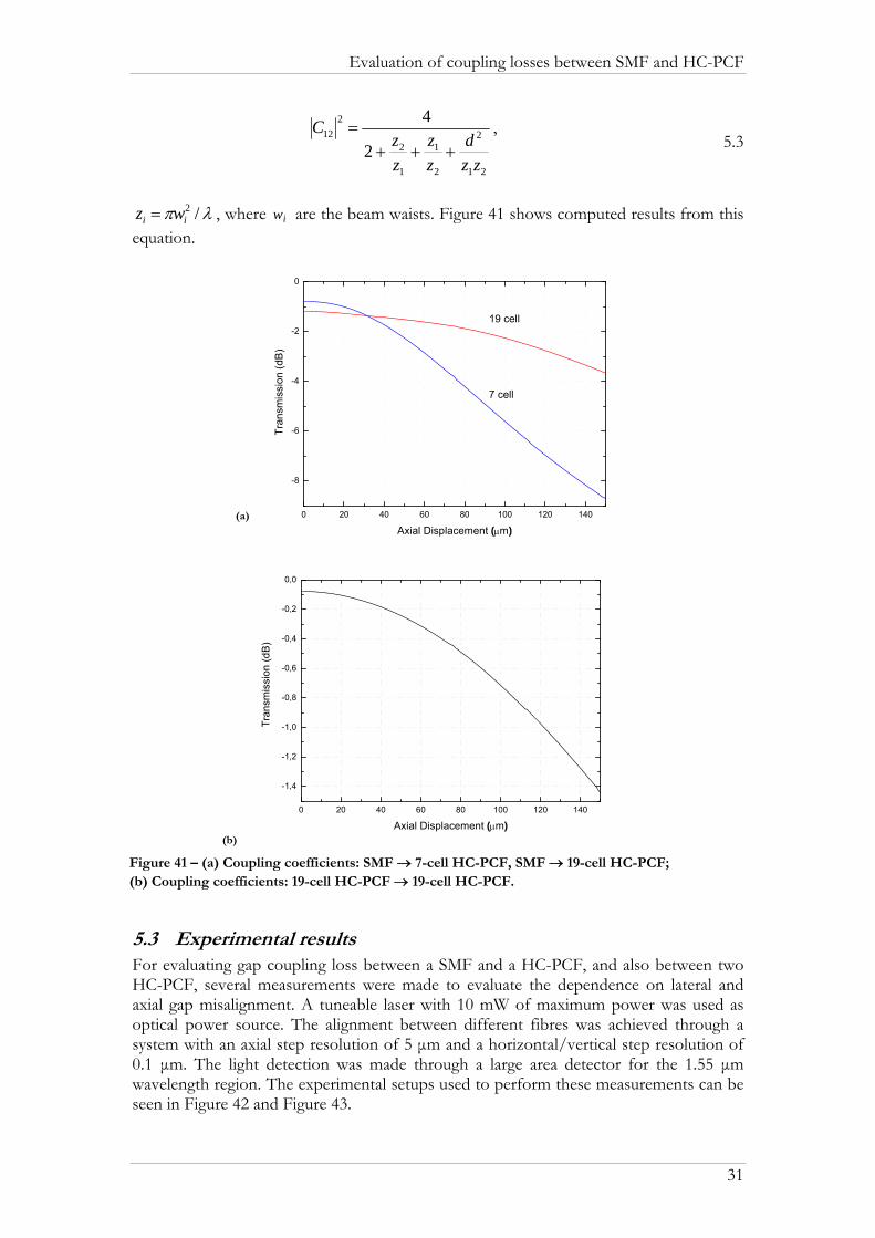
Evaluation of coupling losses between SMF and HC-PCF
31
21
2
2
1
1
2
212
2
4
zzd
zz
zz
C+++
= , 5.3
λπ /2
ii wz = , where w are the beam waists. i Figure 41 shows computed results from this equation.
0 20 40 60 80 100 120 140
-8
-6
-4
-2
0Tr
ansm
issi
on (d
B)
Axial Displacement (μm)
7 cell
19 cell
0 20 40 60 80 100 120 140
-1,4
-1,2
-1,0
-0,8
-0,6
-0,4
-0,2
0,0
Tran
smis
sion
(dB)
Axial Displacement (μm)
Figure 41 – (a) Coupling coefficients: SMF → 7-cell HC-PCF, SMF → 19-cell HC-PCF; (b) Coupling coefficients: 19-cell HC-PCF → 19-cell HC-PCF.
5.3 Experimental results For evaluating gap coupling loss between a SMF and a HC-PCF, and also between two HC-PCF, several measurements were made to evaluate the dependence on lateral and axial gap misalignment. A tuneable laser with 10 mW of maximum power was used as optical power source. The alignment between different fibres was achieved through a system with an axial step resolution of 5 μm and a horizontal/vertical step resolution of 0.1 μm. The light detection was made through a large area detector for the 1.55 μm wavelength region. The experimental setups used to perform these measurements can be seen in Figure 42 and Figure 43.
(a)
(c)
(b)

Evaluation of coupling losses between SMF and HC-PCF
LD PMsmf pcfAligning
point Figure 42 - Setup used for the experimental evaluation of the coupling loss between SMF and HC-PCF.
LD smf pcf pcf PM
Alignedfibres
Aligningpoint
Figure 43 – Setup used for the experimental evaluation of the coupling loss between HC-PCF.
Figure 44 shows the obtained results for axial displacement between SMF and HC-PCF, and between two HC-PCF of the same type. The excess loss values presented are referenced to minimal loss corresponding to direct SMF connection between the laser and the photodetector, in the case of the study of coupling losses between SMF and HC-PCF (setup of Figure 42), and to minimal loss corresponding to direct fibre connection between the previously aligned PCF and the photodetector, in the case of the study of coupling losses between HC-PCF (setup of Figure 43).
(a)
0 10 20 30 40 50 60 70 80 90 100-14
-12
-10
-8
-6
-4
-2
0
SMF to 19-cell HC-PCF 19-cell HC-PCF to 19-cell HC-PCF
Exc
ess
Loss
(dB
)
Axial Displacement (μm)
32
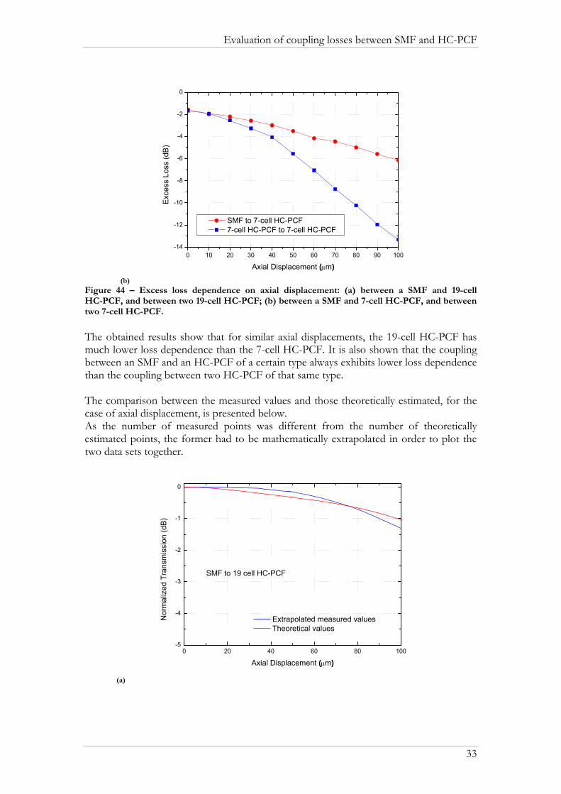
Evaluation of coupling losses between SMF and HC-PCF
(b)
0 10 20 30 40 50 60 70 80 90 100-14
-12
-10
-8
-6
-4
-2
0
SMF to 7-cell HC-PCF 7-cell HC-PCF to 7-cell HC-PCF
Exc
ess
Loss
(dB
)
Axial Displacement (μm)
Figure 44 – Excess loss dependence on axial displacement: (a) between a SMF and 19-cell HC-PCF, and between two 19-cell HC-PCF; (b) between a SMF and 7-cell HC-PCF, and between two 7-cell HC-PCF.
The obtained results show that for similar axial displacements, the 19-cell HC-PCF has much lower loss dependence than the 7-cell HC-PCF. It is also shown that the coupling between an SMF and an HC-PCF of a certain type always exhibits lower loss dependence than the coupling between two HC-PCF of that same type. The comparison between the measured values and those theoretically estimated, for the case of axial displacement, is presented below. As the number of measured points was different from the number of theoretically estimated points, the former had to be mathematically extrapolated in order to plot the two data sets together.
(a)
0 20 40 60 80 100-5
-4
-3
-2
-1
0
Nor
mal
ized
Tra
nsm
issi
on (d
B)
Axial Displacement (μm)
Extrapolated measured values Theoretical values
SMF to 19 cell HC-PCF
33
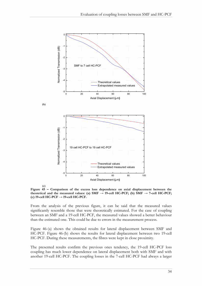
Evaluation of coupling losses between SMF and HC-PCF
(b)
0 20 40 60 80 100-5
-4
-3
-2
-1
0
Nor
mal
ized
Tra
nsm
issi
on (d
B)
Axial Displacement (μm)
Theoretical values Extrapolated measured values
SMF to 7 cell HC-PCF
(c)
0 20 40 60 80 100-5
-4
-3
-2
-1
0
Nor
mal
ized
Tra
nsm
issi
on (d
B)
Axial Displacement (μm)
Theoretical values Extrapolated measured values
19 cell HC-PCF to 19 cell HC-PCF
Figure 45 – Comparison of the excess loss dependence on axial displacement between the theoretical and the measured values: (a) SMF → 19-cell HC-PCF; (b) SMF → 7-cell HC-PCF; (c) 19-cell HC-PCF → 19-cell HC-PCF. From the analysis of the previous figure, it can be said that the measured values significantly resemble those that were theoretically estimated. For the case of coupling between an SMF and a 19-cell HC-PCF, the measured values showed a better behaviour than the estimated one. This could be due to errors in the measurement process. Figure 46-(a) shows the obtained results for lateral displacement between SMF and HC-PCF. Figure 46-(b) shows the results for lateral displacement between two 19-cell HC-PCF. During these measurements, the fibres were kept in close proximity. The presented results confirm the previous ones tendency, the 19-cell HC-PCF loss coupling has much lower dependence on lateral displacement both with SMF and with another 19-cell HC-PCF. The coupling losses in the 7-cell HC-PCF had always a larger
34

Evaluation of coupling losses between SMF and HC-PCF
dependence either on lateral or axial gap misalignment. This behaviour was expected due to the higher mode field diameter of the 19-cell PCF when compared to both the SMF fibre and the 7-cell PCF, which are quite similar. These results indicate that 19-cell HC-PCF is less susceptible to misalignments induced during multiple-coupling gaps implementation or during system operation due to environmental effects.
(a)
0 5 10 15-16
-14
-12
-10
-8
-6
-4
-2
0
Exce
ss L
oss
(dB)
Lateral displacement (μm)
SMF to 19-cell HCF SMF to 7-cell HCF
(b)
0 5 10 15-16
-14
-12
-10
-8
-6
-4
-2
0
SMF to 19-cell HCF 19-cell HCF to 19-cell HCF
Exc
ess
Loss
(dB
)
Lateral Displacement (μm)
Figure 46 – Excess loss dependence on lateral displacement: (a) between a SMF and a 19-cell HC-PCF and between a SMF and a 7-cell HC-PCF; (b) between a SMF and a 19-cell HC-PCF, and between two 19-cell HC-PCF. It was not possible to plot the excess loss dependence on lateral displacement between two 7-cell HC-PCF, due to the huge losses presented. Furthermore, spectral measurements were performed for evaluating splicing losses at different conditions between SMF and 19-cell HC-PCF. Obtained results are presented in Figure 50. From our experiments we concluded that for an arc current around 1-2 power bits (Fujikura FSM-40S internal units) the ideal electric discharge time is around the 300-400 ms, using a splicing technique previously reported [34]. The correspondence between power bits and applied arc current is described in the following plot (Figure 47),
35

Evaluation of coupling losses between SMF and HC-PCF
where the values of current corresponding to 5 and 20 bits, 13.675 mA and 14.2 mA, respectively, were directly obtained from the manufacturer.
4 6 8 10 12 14 16 18 2013,6
13,7
13,8
13,9
14,0
14,1
14,2
current values linear fit
Cur
rent
(mA
)
Arc power (bits)
y = 0,035x + 13,5
Figure 47 – Current (mA) as a function of arc power (bits) for the Fujikura FSM-40S splicing machine So, from the previous plot we can conclude that for 1 and 2 bits the corresponding applied arc current is 13.535 mA and 13.57 mA, respectively. The setup that was used to conduct this experiment is depicted in Figure 48.
Broadbandsource
OSAsmf pcfSplicingmachine
Figure 48 - Experimental setup used to estimate the splice losses between a SMF and 19-cell
HC-PCF The technique employed by the setup of Figure 48 basically consisted in the application of the electric arc discharge mainly over the single mode fibre, in order to avoid the collapsing of the air holes of the HC-PCF. To accomplish the desired results, first, the two fibres were automatically aligned leaving a gap of 25 µm between them, afterwards the splicing machine operating mode was changed to manual mode and the SMF was moved towards the HC-PCF fibre (see Figure 49). After the optimization of their butt-coupling and alignment, the maximum transmitted power between the fibres was registered and set as reference.
36
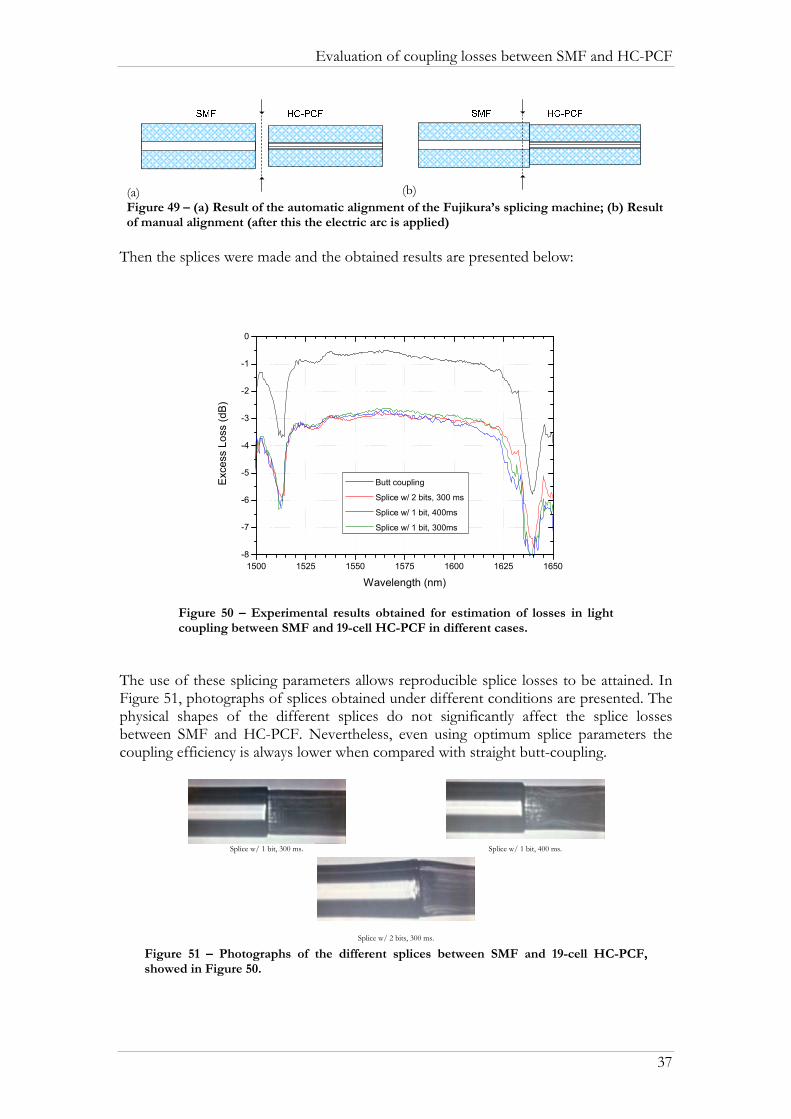
Evaluation of coupling losses between SMF and HC-PCF
(a) (b) Figure 49 – (a) Result of the automatic alignment of the Fujikura’s splicing machine; (b) Result of manual alignment (after this the electric arc is applied)
Then the splices were made and the obtained results are presented below:
37
1500 1525 1550 1575 1600 1625 1650-8
-7
-6
-5
-4
-3
-2
-1
0
Exc
ess
Loss
(dB
)
Wavelength (nm)
Butt coupling
Splice w/ 2 bits, 300 ms
Splice w/ 1 bit, 400ms
Splice w/ 1 bit, 300ms
Figure 50 – Experimental results obtained for estimation of losses in light coupling between SMF and 19-cell HC-PCF in different cases.
The use of these splicing parameters allows reproducible splice losses to be attained. In Figure 51, photographs of splices obtained under different conditions are presented. The physical shapes of the different splices do not significantly affect the splice losses between SMF and HC-PCF. Nevertheless, even using optimum splice parameters the coupling efficiency is always lower when compared with straight butt-coupling.
Splice w/ 1 bit, 300 ms. Splice w/ 1 bit, 400 ms.
Splice w/ 2 bits, 300 ms.
Figure 51 – Photographs of the different splices between SMF and 19-cell HC-PCF, showed in Figure 50.

38
5.4 Summary An analysis of the coupling losses dependence on axial and lateral displacement between SMF and HC-PCF fibres was performed. It was found that 19-cell HC-PCF presents lower coupling losses than 7-cell HC-PCF. In light coupling between HC-PCF of the same type we observed that loss dependence is higher for both axial and lateral misalignments, compared to light coupling between SMF and HC-PCF. However, the obtained results are very encouraging towards the implementation of practical multiple-coupling gaps based gas sensing systems. A simple analysis on splice losses between 19-cell HC-PCF and SMF was also done, being the lowest insertion loss attainable ~2 dB.
Evaluation of coupling losses between SMF and HC-PCF
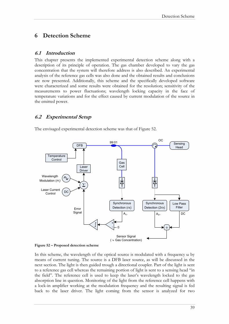
Detection Scheme
6 Detection Scheme
6.1 Introduction This chapter presents the implemented experimental detection scheme along with a description of its principle of operation. The gas chamber developed to vary the gas concentration that the system will therefore address is also described. An experimental analysis of the reference gas cells was also done and the obtained results and conclusions are now presented. Additionally, this scheme and the specifically developed software were characterized and some results were obtained for the resolution; sensitivity of the measurements to power fluctuations; wavelength locking capacity in the face of temperature variations and for the effect caused by current modulation of the source in the emitted power.
6.2 Experimental Setup The envisaged experimental detection scheme was that of Figure 52.
DFB
GasCell
SynchronousDetection (
99:01
A
SensingHead
SynchronousDetection (2
TemperatureControl
WavelengthModulation (
LaserDriver
DCLaser CurrentControl
0+-
ErrorSignal
Low PassFilter
OC
A2 DC
Sensor Signal( Gas Concentration)
Figure 52 – Proposed detection scheme In this scheme, the wavelength of the optical source is modulated with a frequency ω by means of current tuning. The source is a DFB laser source, as will be discussed in the next section. The light is then guided trough a directional coupler. Part of the light is sent to a reference gas cell whereas the remaining portion of light is sent to a sensing head “in the field”. The reference cell is used to keep the laser’s wavelength locked to the gas absorption line in question. Monitoring of the light from the reference cell happens with a lock-in amplifier working at the modulation frequency and the resulting signal is fed back to the laser driver. The light coming from the sensor is analyzed for two
39

Detection Scheme
components. The DC component is filtered out using a low-pass filter and the doubled frequency amplitude modulated signal is isolated using another lock-in amplifier working at 2ω. Division of the amplitude of the 2ω signal by the DC value yields the absorbance and hence the gas concentration. The resulting signal, as observed before, should be independent of power fluctuations. In fact, at an initial stage, as we were neither able to vary gas concentration nor we had a sensing head, it was used a sealed gas cell of known concentration, path length and pressure, instead of a sensing head, so that it was possible to evaluate the system’s behaviour. The setup employing this gas cell can then be seen in the following figure:
DFB
GasCell
SynchronousDetection (
99:01
A
SynchronousDetection (2
TemperatureControl
WavelengthModulation (
LaserDriver
DCLaser CurrentControl
0+-
ErrorSignal
Low PassFilter
A2 DC
Sensor Signal( Gas Concentration)
GasCell
Figure 53 - Gas detection scheme with sensing head substituted by a sealed gas cell This setup is more complicated than that of Figure 26 but it should allow detection limits down to the ppm level. On existing gas detection systems based on the WMS-method, the noise level is mainly determined by interference effects originated in the gas cell. The gas cell acts as a Fabry-Perot cavity, generating interference fringes that disturb the spectral shape. In the case of a HC-PCF-based gas cell, interference effects can be expected as well, since the SMF to HC-PCF interface (silica-air) will also introduce Fresnel reflections. A possible solution to this drawback is presented in chapter 7.3. A setup like the one in Figure 53 was implemented in the C-Band, where it is easier to get components. For the gas cell, a standard acetylene cell was used. This initial system will be helpful on refining the future system at 1.67 µm in terms of noise, loss, sensitivity, etc. Afterwards, a solution to simulate variations in the gas concentration using the sealed gas cell was devised and is presented in the following scheme (Figure 54).
Figure 54 – Setup used to simulate variations in the gas concentration
40

Detection Scheme
Using the setup of Figure 54, variations in the gas concentration would be simulated by the portion of light that would be coupled to the gas cell branch, i.e., if the coupling factor to the branch without the gas cell was represented by a K factor and the emitted power was represented by IO, the power in that branch would be IO.K and the power after the gas cell would be IO.(1-K).α, with α being the gas cell absorption factor (see Figure 55). Therefore, as smaller the K factor the higher the simulated gas concentration would be.
Gas Cell50 : 50I0
KI0.K
I0.(1-K).α
Figure 55 – Simulated variation of gas concentration Unfortunately, this was not a good option, because of light interference between the two coupler branches (Mach-Zender Interferometer). For the DFB source that was being used (Avanex 1905 LMI @ 1530 nm), the coherence length was estimated to be between 40 and 110 m. These values were achieved by the means of the following equations:
λλ
Δ×=
nLC
2
and 6.1
fc
Δ=Δ2λλ , 6.2
with LC being the laser’s coherence length, λ the wavelength, n the refractive index of the medium and c the speed of light in vacuum. The assumed values were: λ = 1530 nm; n = 1.4; c = 3 x 10⁸ m/s; Δf = 2 MHz (typical) or 5 MHz (maximum). Even after an optical fibre with a length higher than 110 m (~500 m) was inserted in one of the coupler’s arms, there was still some interference that could be justified by punctual variations in the source spectral width, Δf. Afterwards, the power of the two branches was independently measured but it was concluded that the total optical power was not constant, this being due to the performance of the variable coupler (Figure 56).
41

Detection Scheme
42
0 10 20 30
2
4
6
8
0
Pow
er (m
W)
Coupling ratio (%) - Newport F-CPL-1550-N-FA
port 1 port 2 port 1 + port 2
Figure 56 – Variable coupler’s output. It is clearly seen that the total optical power is not constant. Consequently, it was concluded that the previous solution was not practical and a gas chamber, where gases could be mixed, was idealized.
6.2.1 Gas chamber A gas chamber, like the one in Figure 57, was developed in order to enable the variation of gas concentrations and to test the implemented setup.
Figure 57 – Computer generated images and photos of the gas chamber
Inside of this chamber there are two U-benches with different path lengths, 30 mm and 6.8 mm. The chamber is hermetically sealed and has one gas input and one gas output, as well as a pressure manometre and an optical feedthrough to allow the passage of the

Detection Scheme
43
fibres (four) to inside of it. Moreover, this chamber will also be helpful for the testing and studying of the HC-PCF-based sensing heads.
6.2.2 Choice of the laser source For the WMS-method, an optical source with the following properties is required: • preferably high power (high power assures good signal-to-noise ratios and allows
many sensors to be multiplexed); • narrow line width (in comparison with the line width of the gas absorption lines,
also insures good signal-to-noise ratios); • tuneable wavelength. Distributed FeedBack lasers (DFB) meet all these demands at affordable cost. A DFB laser is a single frequency laser and thus combines a narrow line width with high power. The line widths of DFB-lasers are typically in the MHz range whereas typical gas line widths are a few GHz. Optical powers are typically in the mW range. A DFB diode can be tuned in wavelength by changing either the temperature (typical tuning rate of 12.5 GHz/K or 100 pm/K @ 1.55 μm) or the operating current (1-2 GHz/mA, or 8-16 pm/mA @ 1.55 μm). While current-tuning is favourable for rapid modulation tasks, thermal tuning has the advantage of providing extremely large mode-hop free tuning ranges (up to 1100 GHz, or 8.8 nm @ 1.55 μm). A drawback of DFB-sources is that the output power may depend on the output wavelength and therefore power fluctuations might occur during a frequency sweep. This is disadvantageous for a measurement which depends on power variations. However, the WMS-method should be able to filter out these source power fluctuations. Therefore, it is clear that a DFB-laser source is the optimal candidate to serve as an optical source for the here envisaged gas sensing system. DFB-lasers are the most common transmitter type in DWDM-systems (Dense Wavelength Division Multiplexing). These systems are commonly used for telecommunication applications and therefore numerous vendors of DFB-lasers can be found. However, in most cases, the available wavelengths are only in the C-band (1525 - 1565 nm) and / or L-band (1570 - 1610 nm) whereas for our methane sensor, a DFB at around 1666 nm is required. Only a few suppliers of DFB-sources in the 1.67 µm wavelength range (telecommunications U-band) could be found: • Fraunhofer Institute for Telecommunications, Heinrich Herz Institute; • NEL NTT Electronics Corporation; • OKI; • Anritsu. Only the sources from the Fraunhofer Institute and those from NEL are available for the 1666 nm wavelength region. The sources from OKI are only available in the 1620-1630 nm and 1645-1655 nm wavelength ranges and therefore are not suited for the envisaged system. The development of Anritsu’s sources in the U-band was discontinued. Both, the Fraunhofer Institute and NEL, were contacted and the requested sources were available off-the-shelf.
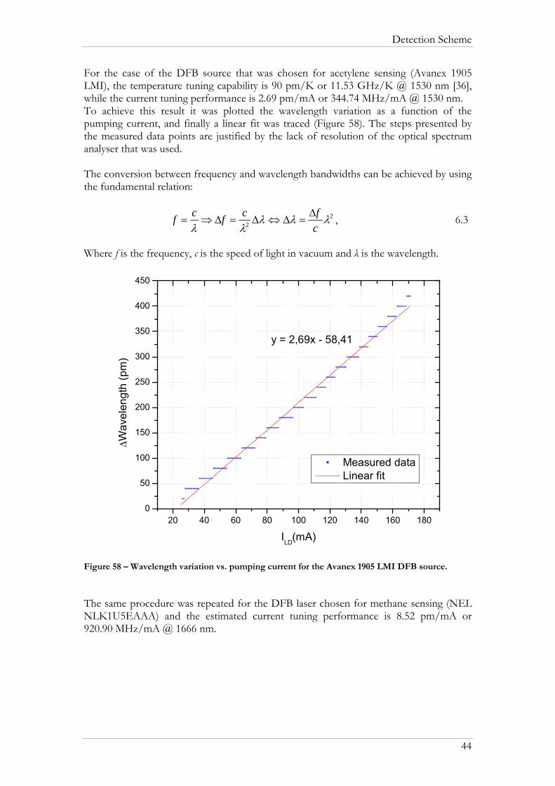
Detection Scheme
For the case of the DFB source that was chosen for acetylene sensing (Avanex 1905 LMI), the temperature tuning capability is 90 pm/K or 11.53 GHz/K @ 1530 nm [36], while the current tuning performance is 2.69 pm/mA or 344.74 MHz/mA @ 1530 nm. To achieve this result it was plotted the wavelength variation as a function of the pumping current, and finally a linear fit was traced (Figure 58). The steps presented by the measured data points are justified by the lack of resolution of the optical spectrum analyser that was used. The conversion between frequency and wavelength bandwidths can be achieved by using the fundamental relation:
22 λλλ
λλ cfcfcf Δ
=Δ⇔Δ=Δ⇒= , 6.3
Where f is the frequency, c is the speed of light in vacuum and λ is the wavelength.
20 40 60 80 100 120 140 160 1800
50
100
150
200
250
300
350
400
450
Measured data Linear fit
ΔWav
elen
gth
(pm
)
ILD(mA)
y = 2,69x - 58,41
Figure 58 – Wavelength variation vs. pumping current for the Avanex 1905 LMI DFB source. The same procedure was repeated for the DFB laser chosen for methane sensing (NEL NLK1U5EAAA) and the estimated current tuning performance is 8.52 pm/mA or 920.90 MHz/mA @ 1666 nm.
44

Detection Scheme
0 20 40 60 80 100 120 140 160 1800
200
400
600
800
1000
1200
1400
Measured data Linear fit
ΔWav
elen
gth
(pm
)
ILD
(mA)
y = 8,52x - 247,54
Figure 59 – Wavelength variation vs. pumping current for the NEL DFB source For the NEL source it was also plotted its wavelength variation as a function of the temperature. For this, the resistance of the temperature controller was varied and the consequent wavelength variation was registered. The resistance values were converted to the corresponding temperatures (in Kelvin) through the following equation♣:
val
val
BRRT
TBRT+
=)ln(
)(
00
0 , 6.4
where (10 kΩ) is the thermistor’s nominal resistance at temperature (298.15 K) and (3410 K) is the thermistor’s energy constant. The results are presented below:
0R 0T
valB
290 300 310 320 330 3400
1000
2000
3000
4000
5000
Measured data Linear fit
ΔW
avel
engt
h (p
m)
Temperature (K)
y = 120x - 35890
Figure 60 – Wavelength variation vs. temperature for the NEL DFB source For the NEL DFB source the estimated temperature tuning capability is 120 pm/K or 12.97 GHz/K @ 1666 nm. ♣ taken from the laser temperature and current controller (Thorlabs ITC 510) manual
45
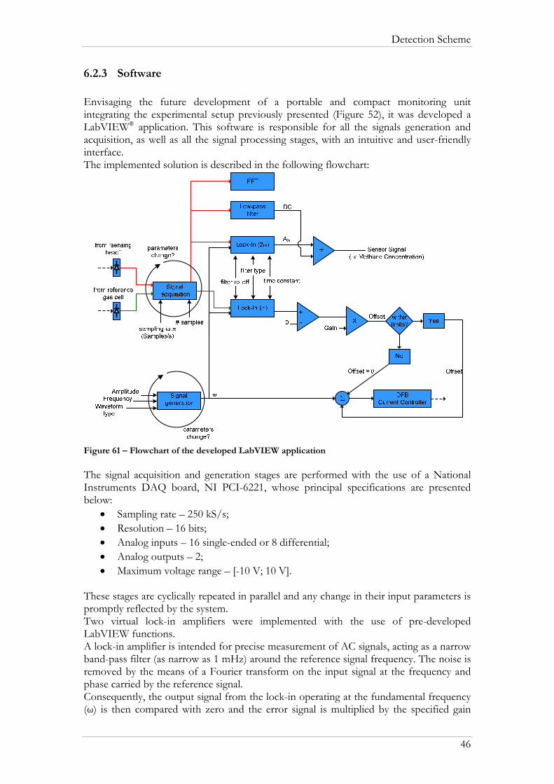
Detection Scheme
6.2.3 Software Envisaging the future development of a portable and compact monitoring unit integrating the experimental setup previously presented (Figure 52), it was developed a LabVIEW® application. This software is responsible for all the signals generation and acquisition, as well as all the signal processing stages, with an intuitive and user-friendly interface. The implemented solution is described in the following flowchart:
Figure 61 – Flowchart of the developed LabVIEW application The signal acquisition and generation stages are performed with the use of a National Instruments DAQ board, NI PCI-6221, whose principal specifications are presented below:
• Sampling rate – 250 kS/s; • Resolution – 16 bits; • Analog inputs – 16 single-ended or 8 differential; • Analog outputs – 2; • Maximum voltage range – [-10 V; 10 V].
These stages are cyclically repeated in parallel and any change in their input parameters is promptly reflected by the system. Two virtual lock-in amplifiers were implemented with the use of pre-developed LabVIEW functions. A lock-in amplifier is intended for precise measurement of AC signals, acting as a narrow band-pass filter (as narrow as 1 mHz) around the reference signal frequency. The noise is removed by the means of a Fourier transform on the input signal at the frequency and phase carried by the reference signal. Consequently, the output signal from the lock-in operating at the fundamental frequency (ω) is then compared with zero and the error signal is multiplied by the specified gain
46

Detection Scheme
value. Afterwards, the result of this operation (offset) is checked to see if it is within a predefined range. In an affirmative case the offset of the generated modulation signal is accordingly adjusted, otherwise, it is considered that the system lost its locked state and the offset is set to zero. To the signal coming from the gas chamber it is applied a similar process, this time at 2ω. The resulting amplitude is then divided by the DC level of the gas chamber signal. An FFT (Fast Fourier Transform) is also applied to the gas chamber signal, enabling the inspection of its harmonic composition and associated signal-to-noise ratios. The interface presented by the application is depicted in the next figure.
Figure 62 – Graphical user interface of the developed application
47

Detection Scheme
6.3 Characterization of the detection scheme
6.3.1 Gas-cells characterization With this analysis we wanted to qualitatively compare different aspects of the gas cells that were being used, such as maximum absorption amplitude, peak width and line shape. In order to obtain the desired information we implemented the following setup:
Figure 63 – Setup used to acquire the absorption spectrum of the gas cells The gas cells that were used in this experiment (2x – 200 Torr; 1x – 400 Torr) only differed in the gas pressure, having an interaction path length of 3 cm and a gas concentration of 100%. With the setup of Figure 63, the absorption line of interest was scanned with 1 pm steps and all the measurements were normalized to the coupler’s branch without the gas cell. The obtained results are depicted in Figure 64 and Figure 65.
1530,2 1530,3 1530,4
-14
-12
-10
-8
-6
-4
-2
0
Nor
mal
ized
abs
orpt
ion
(dB
)
Wavelength (nm)
200 Torr cell - no. 1 200 Torr cell - no. 2 400 Torr cell 200 Torr cells - series
Figure 64 – Absorption spectrum of different gas cells using different configurations Analyzing the traces of Figure 64, we can state that the two 200 Torr cells were identical and that increasing the interaction length between light and gas (associating the two cells
48
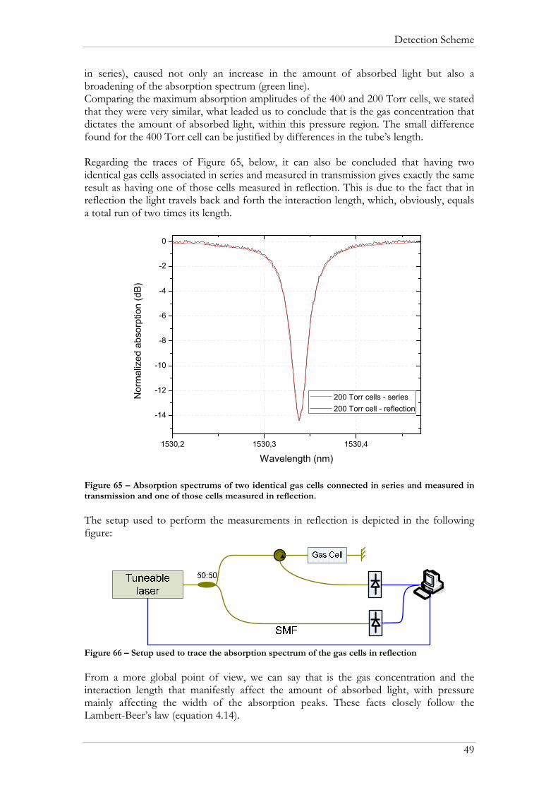
Detection Scheme
in series), caused not only an increase in the amount of absorbed light but also a broadening of the absorption spectrum (green line). Comparing the maximum absorption amplitudes of the 400 and 200 Torr cells, we stated that they were very similar, what leaded us to conclude that is the gas concentration that dictates the amount of absorbed light, within this pressure region. The small difference found for the 400 Torr cell can be justified by differences in the tube’s length. Regarding the traces of Figure 65, below, it can also be concluded that having two identical gas cells associated in series and measured in transmission gives exactly the same result as having one of those cells measured in reflection. This is due to the fact that in reflection the light travels back and forth the interaction length, which, obviously, equals a total run of two times its length.
1530,2 1530,3 1530,4
-14
-12
-10
-8
-6
-4
-2
0
Nor
mal
ized
abs
orpt
ion
(dB)
Wavelength (nm)
200 Torr cells - series 200 Torr cell - reflection
Figure 65 – Absorption spectrums of two identical gas cells connected in series and measured in transmission and one of those cells measured in reflection. The setup used to perform the measurements in reflection is depicted in the following figure:
Figure 66 – Setup used to trace the absorption spectrum of the gas cells in reflection From a more global point of view, we can say that is the gas concentration and the interaction length that manifestly affect the amount of absorbed light, with pressure mainly affecting the width of the absorption peaks. These facts closely follow the Lambert-Beer’s law (equation 4.14).
49

Detection Scheme
6.3.2 Results invariance in the presence of power fluctuations In order to evaluate the effect of power fluctuations in the system output, it was inserted an optical variable attenuator before the gas cell we used for measurements (see Figure 67).
Figure 67 – Setup with optical variable attenuator to evaluate the influence of power fluctuations in the sensor signal For different amplitudes and frequencies of modulation, we varied the induced
attenuation and registered the resulting DCA w2 ratio values.
0 2 4 6 8 10 12 140,0
0,2
0,4
0,6
0,8
1,0
Nor
mal
ized
A2ω
/DC
Induced Attenuation (dB)
75 mV - 1 KHz 75 mV - 2 KHz 75 mV - 5 KHz 50 mV - 1 KHz 50 mV - 2 KHz 100 mV - 1 KHz 100 mV - 2 KHz
Figure 68 – Analysis of the influence of power attenuation in the system’s response
50

Detection Scheme
As can be seen in the previous figure, the system response remains fairly unaltered for attenuations smaller than 6 dB. For the different amplitudes and frequencies of modulation, there are no major differences to notice, however it can be said that, in the implemented system, greater modulation amplitudes along with lower modulation frequencies yield better overall results. This is due to the bandwidth (~4 kHz) of the powermeter (Agilent 81532A) and to the fact that a greater modulation amplitude will consequently result in a higher amplitude signal, thus being less susceptible to power variations. These assumptions can be supported by the analysis of the resulting signals from the plot of Figure 68. It can be seen that for 15 dB of induced attenuation the signals modulated with 75 mV of amplitude, for the same frequencies, were more susceptible to the attenuation than the signals modulated with 100 mV of amplitude. The same is verified when comparing the 50 mV to the 75 mV case. However, the result of a signal modulated with an amplitude of 75 mV and a frequency of 5 kHz is much more susceptible to losses than the signals of the same amplitude with lower frequencies. The occurrence of frequency duplication, caused by the emission centred in the absorption peak, of the 5 kHz signal will result in a signal outside the bandwidth of the powermeter giving raise to the facts here noticed.
6.3.3 Feedback-loop response to perturbations Another aspect that was subject of our study was the response to perturbations of the feedback-loop used for locking the emission wavelength to the desired absorption peak. For this, we induced, to the laser, a temperature variation and registered the system response. Here, the DC level of the modulating signal suffered constant adjustments in order to make the signal measured by the lock-in, at the frequency ω, as close to zero as possible, thus indicating that the emission was centred in the gas absorption peak. Different gain values were tested. For each iteration, blocks of 8192 samples at a sampling frequency of 50 kS/s were acquired.
0 50 100 150 200 250 300 350 400 450-0,008
-0,006
-0,004
-0,002
0,000
0,002
0,004
0,006
Aω
Time (a.u.)
a) Feedback-loop response for a gain of 0.1
0 50 100 150-0,008
-0,006
-0,004
-0,002
0,000
0,002
0,004
0,006
Aω
Time (a.u.)
b) Feedback-loop response for a gain of 0.5
51

Detection Scheme
0 50 100 150-0,008
-0,006
-0,004
-0,002
0,000
0,002
0,004
0,006
0,008
0,010
Aω
Time (a.u.)
c) Feedback-loop response for unit gain
0 50 100-0,008
-0,006
-0,004
-0,002
0,000
0,002
0,004
0,006
0,008
0,010
Aω
Time (a.u.)
d) Feedback-loop response for a gain of 2
0 50 100 150 200-0,008
-0,006
-0,004
-0,002
0,000
0,002
0,004
0,006
0,008
Aω
Time (a.u.)
e) Feedback-loop response for a gain of 3
Figure 69 – Feedback-loop responses for different gain values For a gain higher than 3, the system became unstable and so its purpose was no longer achieved. For the configuration here tested, we concluded that the unit gain was the ideal one, since it enabled the quickest recovery of the system without any overshoot.
6.3.4 Laser power modulation In order to evaluate the effect of the current modulation in the emitted power, it was connected a DC source to the current modulation input and registered the variations that changes in the DC value caused in the emitted power.
-0,8 -0,6 -0,4 -0,2 0,0 0,2 0,4 0,6 0,8-15
-10
-5
0
5
1530,2
1530,3
1530,4
1530,5
1530,6
Power (dBm)
λ (n
m)
Pow
er (d
Bm
)
DC (V)
λ(nm)
Figure 70 – Power and wavelength variation with current modulation
52
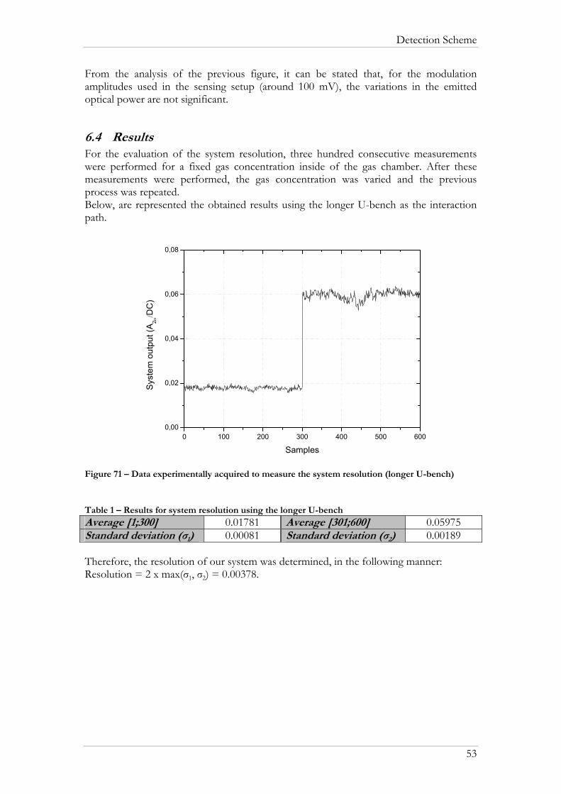
Detection Scheme
From the analysis of the previous figure, it can be stated that, for the modulation amplitudes used in the sensing setup (around 100 mV), the variations in the emitted optical power are not significant.
6.4 Results For the evaluation of the system resolution, three hundred consecutive measurements were performed for a fixed gas concentration inside of the gas chamber. After these measurements were performed, the gas concentration was varied and the previous process was repeated. Below, are represented the obtained results using the longer U-bench as the interaction path.
0 100 200 300 400 500 6000,00
0,02
0,04
0,06
0,08
Sys
tem
out
put (
A2ω
/DC
)
Samples
Figure 71 – Data experimentally acquired to measure the system resolution (longer U-bench) Table 1 – Results for system resolution using the longer U-bench Average [1;300] 0.01781 Average [301;600] 0.05975 Standard deviation (σ1) 0.00081 Standard deviation (σ2) 0.00189 Therefore, the resolution of our system was determined, in the following manner: Resolution = 2 x max(σ1, σ2) = 0.00378.
53

Detection Scheme
For the shorter U-bench the results were as follows:
0 100 200 300 400 500 6000,000
0,002
0,004
0,006
0,008
0,010
0,012
0,014
0,016
0,018
Syst
em o
utpu
t (A
2ω/D
C)
Samples
Figure 72 - Data experimentally acquired to measure the system resolution (shorter U-bench) Table 2 - Results for system resolution using the shorter U-bench Average [1;300] 0.00454 Average [301;600] 0.015 Standard deviation (σ1) 0.00189 Standard deviation (σ2) 0.00068 In a similar way it was concluded that the system resolution using the shorter U-bench was 0.00378. For each gas concentration and U-bench, it was also measured the quantity of absorbed light with the following setup:
Figure 73 – Setup used to measure the amount of absorbed light by the gas inside of the chamber
54

Detection Scheme
The obtained results are presented below:
1530,1 1530,2 1530,3 1530,4 1530,5 1530,6-5
-4
-3
-2
-1
0
lower gas concentration higher gas concentration
Longer U-bench
Nor
mal
ized
abs
orpt
ion
(dB
)
Wavelength (nm)
Figure 74 – Absorption spectrum obtained with the setup of Figure 73 (longer U-bench)
1530,1 1530,2 1530,3 1530,4 1530,5 1530,6-5
-4
-3
-2
-1
0
Nor
mal
ized
abs
orpt
ion
(dB)
Wavelength (nm)
lower gas concentration higher gas concentration
Shorter U-bench
Figure 75 - Absorption spectrum obtained with the setup of Figure 73 (shorter U-bench) From the previous results we concluded that with our experimental setup and software application it was in fact possible to qualitatively monitor variations in gas concentration.
55

Detection Scheme
56
6.5 Summary Within this chapter a description of the experimental implemented detection scheme was made. A configuration employing a variable coupler was implemented and tested but it was concluded that this solution did not suit our needs and was consequently abandoned. Therefore, in order to allow the variation and of gas concentration and further test the implemented setup, a gas chamber was idealized. This gas chamber, simultaneously, will be helpful on the testing of the future sensing heads, made with microstructured fibres. Afterwards, it was justified the choice of a DFB source for our spectroscopy application and the chosen sources were characterized. Having in mind the future implementation of the experimental setup as a portable and compact unit, a LabVIEW® application was developed. A description of all the signal generation and acquisition along with all the signal processing, performed by this software, was also provided. Furthermore, the reference gas cells were characterized and it was concluded that the gas concentration and the length of interaction represent the most important factors in light absorption. The system sensitivity to power fluctuations was also analysed and the results showed that the experimental setup closely followed the expected results, i.e., the system output was practically invariant regardless of the applied power attenuations. Next, the DFB emission was forced to move away from the absorption peak wavelength and the feedback-loop capability of recovery to the locked-state was analysed. It was concluded that the feedback-loop served the intended purpose and that the gain value directly affects the recovery time and overshoot. The modulation of the source power caused by its current modulation was also analysed and it was concluded that for the used modulating amplitudes it was not noteworthy. Finally, the experimentally achieved value for the system’s resolution was 0.00378.
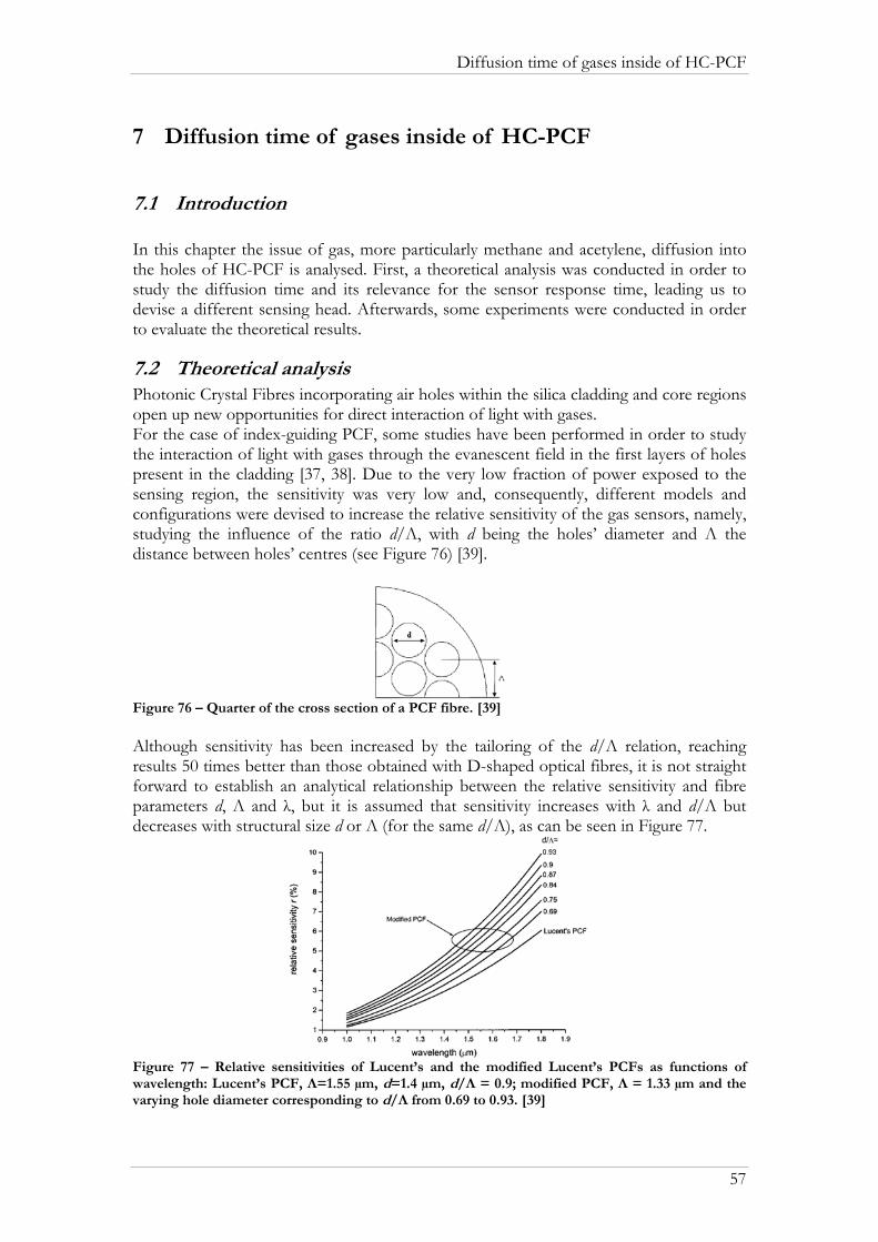
Diffusion time of gases inside of HC-PCF
7 Diffusion time of gases inside of HC-PCF
7.1 Introduction In this chapter the issue of gas, more particularly methane and acetylene, diffusion into the holes of HC-PCF is analysed. First, a theoretical analysis was conducted in order to study the diffusion time and its relevance for the sensor response time, leading us to devise a different sensing head. Afterwards, some experiments were conducted in order to evaluate the theoretical results.
7.2 Theoretical analysis Photonic Crystal Fibres incorporating air holes within the silica cladding and core regions open up new opportunities for direct interaction of light with gases. For the case of index-guiding PCF, some studies have been performed in order to study the interaction of light with gases through the evanescent field in the first layers of holes present in the cladding [37, 38]. Due to the very low fraction of power exposed to the sensing region, the sensitivity was very low and, consequently, different models and configurations were devised to increase the relative sensitivity of the gas sensors, namely, studying the influence of the ratio d/Λ, with d being the holes’ diameter and Λ the distance between holes’ centres (see Figure 76) [39].
Figure 76 – Quarter of the cross section of a PCF fibre. [39] Although sensitivity has been increased by the tailoring of the d/Λ relation, reaching results 50 times better than those obtained with D-shaped optical fibres, it is not straight forward to establish an analytical relationship between the relative sensitivity and fibre parameters d, Λ and λ, but it is assumed that sensitivity increases with λ and d/Λ but decreases with structural size d or Λ (for the same d/Λ), as can be seen in Figure 77.
Figure 77 – Relative sensitivities of Lucent’s and the modified Lucent’s PCFs as functions of wavelength: Lucent’s PCF, Λ=1.55 µm, d=1.4 µm, d/Λ = 0.9; modified PCF, Λ = 1.33 µm and the varying hole diameter corresponding to d/Λ from 0.69 to 0.93. [39]
57

Diffusion time of gases inside of HC-PCF
The relative sensitivity coefficient is defined as:
fnnr er )/(= , 7.1 where nr is the index of the gas species and is approximately equal to 1, ne is the effective index of the guided mode and f is the fraction of the total power located in the holes. For the case of hollow-core PCF, as we’re concerned, the core is where most of the power is guided and is effectively possible to create a greater interaction path between light and gas or liquids. In order to develop a HC-PCF-based gas sensor, allowing direct interaction of light with gases within its structure, there is the need to study the diffusion of gas inside of the fibres. For the previous purpose, let’s consider we have an HC-PCF fibre with one open butt-end immersed in a methane atmosphere and the other butt-end closed. Methane gradually penetrates the fibre by diffusion. We characterize the diffusion by relative concentration of gas inside the fibre averaged over the fibre length. This concentration can be found by integration of local concentration that is obtained by solving the diffusion equation with corresponding boundary conditions. For the average relative concentration we use the following expression, represented in a form of an infinite sum [39]:
2
2 21,3,5
8 11 exp2j
jC Dj l
ππ
∞
=
t⎡ ⎤⎛ ⎞= − − ⋅⎢ ⎥⎜ ⎟
⎝ ⎠⎢ ⎥⎣ ⎦∑ , 7.2
where l is the fibre length, D is the diffusion coefficient of methane and t is the time. The diffusion coefficient for methane in nitrogen is m2s-1 [40]. Using this value, the dependence of the average relative concentration on time for four fibre lengths (0.02, 0.06, 0.18, and 0.54 m) was plotted. The result is shown in
5102.2 −×
Figure 78.
0 50 100 150 200 250 3000,0
0,2
0,4
0,6
0,8
1,0
Ave
rage
rela
tive
conc
entra
tion
Time (s)
0,02 m 0,06 m 0,18 m 0,54 m
Figure 78 – Time-dependence of the average relative methane concentration inside different lengths of HC-PCF, having a single open end.
58

Diffusion time of gases inside of HC-PCF
The following graph represents the time-dependence of the average relative methane concentration inside different HC-PCF, this time having two open ends. Now, the fibre length is considered just once and this change is reflected in equation 7.2 in the following manner:
∑∞
= ⎥⎥⎦
⎤
⎢⎢⎣
⎡⋅⎟
⎠⎞
⎜⎝⎛−−=
5,3,1
2
22 exp181j
tDlj
jC π
π. 7.3
0 50 100 150 200 250 3000,0
0,2
0,4
0,6
0,8
1,0
Ave
rage
rela
tive
conc
entra
tion
Time (s)
0,02 m 0,06 m 0,18 m 0,54 m
Figure 79 - Time-dependence of the average relative methane concentration inside different lengths of HC-PCF, having two open ends. Table 3, below, gives the time needed to obtain a 90% average concentration of methane in the four example lengths considered for the HC-PCF in the previous graphs. Table 3 - Expected time to obtain 90% average methane concentration for different HC-PCF lengths
One open end Two open ends l (m) t (s) t (min) t (s) t (min) 0.02 16 0.27 4 0.07 0.06 136 2.27 34 0.57 0.18 1220 20.33 305 5.08 0.54 10980 183 2745 45.75
It should be mentioned that on these calculations, surface effects were neglected, given the considerably large diameter of the core of the HC-PCF (in comparison to the gas molecules’ size). In fact, results must not be very different if one considers 7-cell or 19-cell HC-PCF. For the case of acetylene gas, similar studies were conducted and the results are pictured below. The gas diffusion coefficient that was considered for acetylene was
m2s-1[41]. 5107774.1 −×=D
59

Diffusion time of gases inside of HC-PCF
0 50 100 150 200 250 3000,0
0,2
0,4
0,6
0,8
1,0
Ave
rage
rela
tive
conc
entra
tion
Time (s)
0,02 m 0,06 m 0,18 m 0,54 m
Figure 80 - Time-dependence of the average relative acetylene concentration inside different lengths of HC-PCF, having a single open end.
0 50 100 150 200 250 3000,0
0,2
0,4
0,6
0,8
1,0
Ave
rage
rela
tive
conc
entra
tion
Time (s)
0,02 m 0,06 m 0,18 m 0,54 m
Figure 81 - Time-dependence of the average relative acetylene concentration inside different lengths of HC-PCF, having two open ends. As for the case of methane, Table 4, below, gives the time needed to obtain a 90% average concentration of acetylene in the four example lengths considered for the HC-PCF in the previous graphs. Table 4 - Expected time to obtain 90% average acetylene concentration for different HC-PCF lengths
One open end Two open ends l (m) t (s) t (min) t (s) t (min) 0.02 19 0.32 5 0.08 0.06 168 2.8 42 0.7 0.18 1510 25.17 378 6.3 0.54 13590 226.5 3398 56.63
60

Diffusion time of gases inside of HC-PCF
61
From the analysis of the previous results, we can conclude that the length of the fibre used as the sensing head will directly affect the response time of the desired system, limiting the time that gases may take to diffuse into the holes. As expected, it was also concluded that with two open ends the gas diffusion inside of the microstructured fibres happens much faster than with a single open end. So, in order to improve the system sensitivity without compromising the response time, the introduction of periodic openings along the sensing head fibre was devised.
Figure 82 - Sensing head with periodic openings in the PCF fibre.
7.3 Experimental Results In order to practically evaluate the theoretical analysis presented before, some experiments were conducted. So, the main idea was to align a segment of HC-PCF with SMF, effectively transmit light through the segment and then inject gas into the chamber and register the decay of transmitted light with time, caused by the absorbance of the gas inside of the HC-PCF. The implemented setup is described in the following figure:
DFBSMF SMF
Gas Chamber
HC-PCF
Gas input Gas output Photodetector
Figure 83 – Setup used to measure the diffusion time of gas inside of HC-PCF The DFB source was emitting at one of the gas absorption peaks (~1666 nm for the case of methane and ~1530 nm for the case of acetylene). Besides the need for the correct alignment there was also the need of creating a gap through which the gas would diffuse into the HC-PCF. Then, the devised solution consisted in the use of ferrules along with slitted sleeves (see Figure 84), since these are standard and common components, easy to find and of reduced price.
Figure 84 – Photo of two ferrules connected and aligned by a zirconia sleeve with a slit

Diffusion time of gases inside of HC-PCF
The alignment of the HC-PCF inside of the ferrules was performed with nanometre resolution positioning stages and below are presented some photos of the setup and of the results.
Figure 85 – Overview of the setup used to align the HC-PCF inside of the ferrules
Figure 86 – Detailed image of the setup used for alignment of the HC-PCF inside of the ferrules
Figure 87 – Photo with detailed view of the HC-PCF alignment inside of the ferrule
62
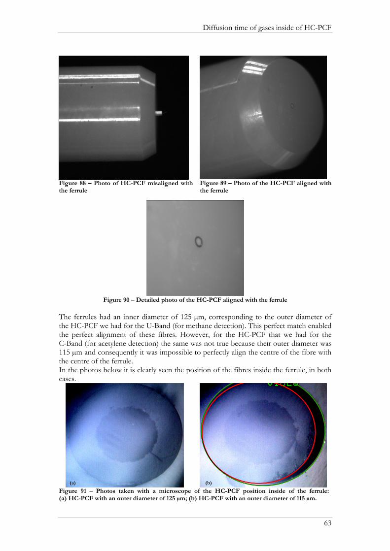
Diffusion time of gases inside of HC-PCF
63
Figure 88 – Photo of HC-PCF misaligned with the ferrule
Figure 89 – Photo of the HC-PCF aligned with the ferrule
Figure 90 – Detailed photo of the HC-PCF aligned with the ferrule
The ferrules had an inner diameter of 125 µm, corresponding to the outer diameter of the HC-PCF we had for the U-Band (for methane detection). This perfect match enabled the perfect alignment of these fibres. However, for the HC-PCF that we had for the C-Band (for acetylene detection) the same was not true because their outer diameter was 115 µm and consequently it was impossible to perfectly align the centre of the fibre with the centre of the ferrule. In the photos below it is clearly seen the position of the fibres inside the ferrule, in both cases.
Figure 91 – Photos taken with a microscope of the HC-PCF position inside of the ferrule: (a) HC-PCF with an outer diameter of 125 µm; (b) HC-PCF with an outer diameter of 115 µm.
(a) (b)

Diffusion time of gases inside of HC-PCF
This misalignment presented by the fibre working in the C-Band disabled the possibility of experimentally evaluate the diffusion time of acetylene inside of HC-PCF. Fortunately, the same was not true for the fibre in the U-Band and some experiments were conducted to evaluate the diffusion time of methane inside of HC-PCF. It was used the setup of Figure 83, and it was injected into the chamber a mixture of 5% of methane and 95% of nitrogen. The transmittance was measured every second and the fibre length was 13.7 cm. The gap between the SMF and the HC-PCF, to allow the gas diffusion into the HC-PCF, was guaranteed by the use of angled ferrules (FC/APC) in the side of the SMF fibre. These ferrules, exhibiting an angle of 8º, were chosen because they do not permit Fresnel (silica-air interface) back-reflections to be guided. The gap between SMF and HC-PCF was ~176 µm (represented by “x” in Figure 92). This gap can even be smaller since there are other ferrule configurations.
Figure 92 – Sketch of the gap between an 8º angled ferrule and a flat ferrule Below is presented the normalized measured data.
0 100 200 300 4000,00
0,9
1,0
Nor
mal
ized
tran
smitt
ance
Time (s)
Figure 93 – Experimental results for the diffusion time of 5% of methane inside of a HC-PCF (with two open ends) From the analysis of the graph it can be stated that the time taken to achieve 95% of the steady-state was about 248 s, while the theoretically predicted value was about 233 s, thus leading to a relative error of ~6%. This result strongly followed the expected one and confirmed the reliability of the adopted model. Our colleagues from IPHT-Jena, in Germany, who are also part of the NextGenPCF consortium, also conducted some experiments in order to evaluate the diffusion time of CH4 inside of microstructured fibres.
64
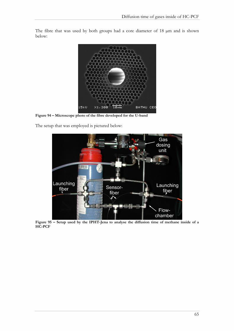
Diffusion time of gases inside of HC-PCF
65
The fibre that was used by both groups had a core diameter of 18 µm and is shown below:
Figure 94 – Microscope photo of the fibre developed for the U-band The setup that was employed is pictured below:
Figure 95 – Setup used by the IPHT-Jena to analyse the diffusion time of methane inside of a HC-PCF

Diffusion time of gases inside of HC-PCF
66
The results that were obtained, with a 1.25 m piece of HC-PCF, are presented in the next figure:
Figure 96 – Experimental results for the diffusion time of 100% of CH4 inside of a HC-PCF (with two open ends) From the analysis of the previous results we could conclude that the values now obtained were quite different from those theoretically calculated (~323 min), with a relative error of ~29.7%. This fact can be explained by not considering the temperature and wall-effect in our theoretical calculations. The core diameter of the fibres used in both experiments was 18 µm. The influence of wall-effect, also analysed by the IPHT-Jena group, is presented in the following results, where the measured and predicted diffusion times for different lengths of HC-PCF are plotted, with and without taking into account the wall-effect, for different temperatures.
0 50 100 150 2000
6
12
18
24
predicted: T=273 K, with wall effect T=273 K, no wall effect T=313 K, with wall effect T=313 K, no wall effect
measured (T= ca.300 K)
Sens
or re
spon
se ti
me
t 95%
(h
)
Sensor fiber length (cm) Figure 97 – Wall-effect and temperature effect in the diffusion time of gas inside of different lengths of HC-PCF
0 1 2 3 4 5 6 7 8 9 10 11 1
1x10-11
2x10-11
3x10-11
4x10-11
5x10-11
2
t95= 460 min
o ,65 µm wavelength (low res.)
Time [h]
pt. power at 1
opt.
pow
er [W
]Tr
ansm
itted
pow
er (W
) Acquired data

Diffusion time of gases inside of HC-PCF
67
It can be seen that the measured results closely fell within expected and that wall-effect is reflected by an increase in gas diffusion time. However, for the small length segments intended to be used in the sensing head the wall-effect is practically negligible. Some considerations on the effect of temperature in gas diffusion times can also be taken from the traces of Figure 97. The higher the temperature, the faster the gas diffusion. This makes sense as an increase in temperature is translated into an increase in the kinetic energy of the gas molecules.
7.4 Summary After a theoretical analysis on the diffusion time of gas inside of hollow-core fibres it was concluded that the length of the HC-PCF segments used as the sensing head will critically define the response time of the sensing system, because of the direct relation between fibre length and gas diffusion time inside of it. Then, the introduction of periodic openings along the sensing fibre was devised since it will, therefore, improve the system’s sensitivity without compromising the system’s response time. The use of standard ferrules and sleeves in the coupling of the multiple segments of fibre proved to be promising, but special attention should be placed in the components dimensions since very small misalignments reveal to be critical in the system’s behaviour. The use of angled ferrules is useful in the way they prevent Fresnel back-reflections to be guided and consequently damage the source or induce perturbations in the measured signals. The obtained experimental results were helpful as they followed the predicted ones and stressed the relevance of the wall-effect and temperature in the diffusion time of gases, for longer fibre lengths.

Portable Monitoring Unit
8 Portable Monitoring Unit
8.1 Introduction A compact multi-sensor monitoring unit is already being designed and implemented and the final system will present itself as a portable unit integrating a computer (motherboard, memory, hard-disk, touch-screen…) and an optical-electrical board that will implement the scheme of Figure 99.
Figure 98 – 3D computer model of the portable monitoring unit that is being implemented The previously described LabVIEW® application will, therefore, be further developed and adjusted to control all the unit system and present a graphical interface to the user. The optical-electrical system that will be implemented is depicted in the next page.
68

Portable Monitoring Unit
DFB
GasCell
SynchronousDetection (
99:01
A
SynchronousDetection (2
TemperatureControl
WavelengthModulation (
LaserDriver
DCLaser CurrentControl
0+-
ErrorSignal
Low PassFilter
OC
A2 DC
Sensor Signal( Gas Concentration)
SensingHead
FBG
FBG
OS
SensingHead
Figure 99 – Optical-electrical scheme for the interrogation unit As depicted in the previous figure, measurements will be performed in reflection, employing an optical switch, to temporally multiplex the channels, and Bragg gratings tuned to the desired wavelengths.
Figure 100 – Schematic diagram of the monitoring unit and sensing head for the case of measurements performed in reflection
69

Portable Monitoring Unit
The optical-electrical board that will be included in the portable unit is also being implemented and will have the following aspect:
Figure 101 – Optical-electrical board that is being implemented to the portable unit
8.2 Distributed Sensing Alternatives An alternative to the solution described in the previous section is that the gas sensors could be placed in series to do a distributed measurement. For this, one could combine the WMS-method with Time Division Multiplexing (TDM). This method requires Fibre Bragg Gratings (FBG), which act like point-like mirrors in the fibre. The position of the FBG in the fibre can be determined from the time it takes for the light signal to travel back and forth in the optical fibre (similar to a radar-echo). For this, the light source needs to be pulsed with pulse lengths in the range of nanoseconds for meter-sized position resolutions. Also, the WMS-method needs to be configured in reflection mode rather than in transmission. The amount of reflected light can be tuned by the FBG (from a few percent to >90% reflectivity), depending on the amount of required reflected optical power. Based on the optical loss of the PCF-based sensor, the FBG-reflectivity could be chosen: • When the power loss in each sensor is small, there is a gradual decrease in power all along the fibre. In this case, all sensors can be put in series and low reflectivity FBG need to be used.
Figure 102 – Sensors distributed in series along a fibre.
70
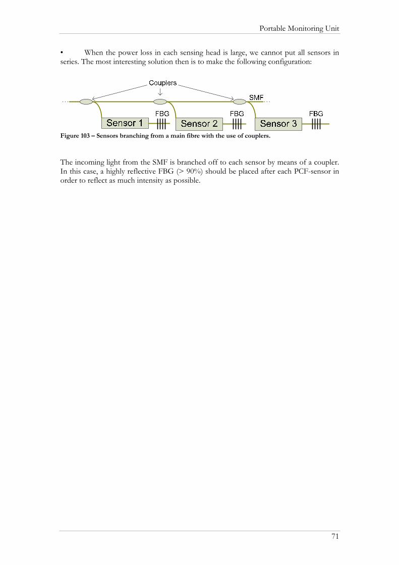
Portable Monitoring Unit
• When the power loss in each sensing head is large, we cannot put all sensors in series. The most interesting solution then is to make the following configuration:
Figure 103 – Sensors branching from a main fibre with the use of couplers. The incoming light from the SMF is branched off to each sensor by means of a coupler. In this case, a highly reflective FBG (> 90%) should be placed after each PCF-sensor in order to reflect as much intensity as possible.
71
Conclusions
72
9 Conclusions Despite the apparent diversity of subjects presented in this thesis, it is easily recognized the existence of a common conducting path to all the work: the development of remote gas sensing systems using Photonic Crystal Fibres (PCF). PCF present themselves as an enabling component that has dramatically pushed forward the frontiers of optical fibres which in turn has opened the doors to many promising applications, such has the development of supercontinuum white light sources for cytology, high-power fibre lasers and low bending losses fibres to fibre-to-the-home. Concerning remote gas sensing, PCF extend their capabilities to the detection and measurement of small gas sample volumes in the vicinities of pipelines, landfills and mining sites, where the increase of gas concentration can naturally occur and consequently reach explosive limits. Moreover, the development of hollow-core PCF based gas sensing systems enable the direct interaction of light with gases, what consequently results in an intrinsically explosion safe solution since the risk of electrical spark ignition does not exist. Monitoring of multiple sensing points is another advantage presented by these systems. Light coupling between conventional SMF and different types of HC-PCF has also been studied. Losses induced by axial and lateral misalignments have been experimentally evaluated and promising results were attained, being the 19-cell HC-PCF the one with most interesting overall performance. The splice between SMF and HC-PCF has been optimized and losses as low as ~2 dB were achieved. Gas diffusion time inside of HC-PCF was also studied and along with the experimentally obtained results it was concluded that the fibre length directly affects the gas diffusion time inside of it and, consequently, the response time of HC-PCF based gas sensors. Furthermore, the delay introduced by gas diffusion into the fibre (~34 s for methane diffusion on a 6 cm segment) does not constitute a drawback for the intended application since gas concentrations are not expected to change dramatically over such short notice. Further work on reducing the sensor response time would be rather meaningless. Subsequently, the use of multiple gap coupled HC-PCF segments was devised since it is a practical way of improving the system sensitivity without compromising the response time. However, special attention should be considered for the components dimensions and alignment. An experimental gas sensing setup based on Wavelength Modulation Spectroscopy was implemented and proved to be a reliable option for the intended purpose. Afterwards, a software application was developed to control this setup and handle all the signal processing, generation and acquisition tasks. The obtained results were very encouraging towards the development of a portable and compact remote gas monitoring unit that is already being designed and implemented. A resolution of 0.00378 for the system output was obtained using the experimental setup along with the developed software, thus showing that the qualitative monitoring of small changes in gas concentration is in fact possible. In the future, further work should be conducted in order to quantify gas concentration and, accordingly, evaluate the system sensitivity. The portable monitoring unit will continue to be developed and, as one of the project goals, the final results and developed solution will be licensed. Negotiations between INESC Porto and one of its spin-off companies, FiberSensing, have already been initiated. FiberSensing supplies advanced monitoring systems based in optical fibre sensors.

10 Appendixes
A Poster accepted for the European Workshop on Optical Fibre Sensors – 2007
73
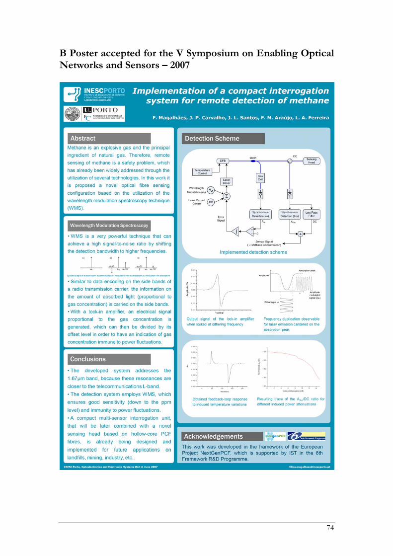
B Poster accepted for the V Symposium on Enabling Optical Networks and Sensors – 2007
74

C Oral presentation on V Symposium on Enabling Optical Networks and Sensors – 2007
75

76
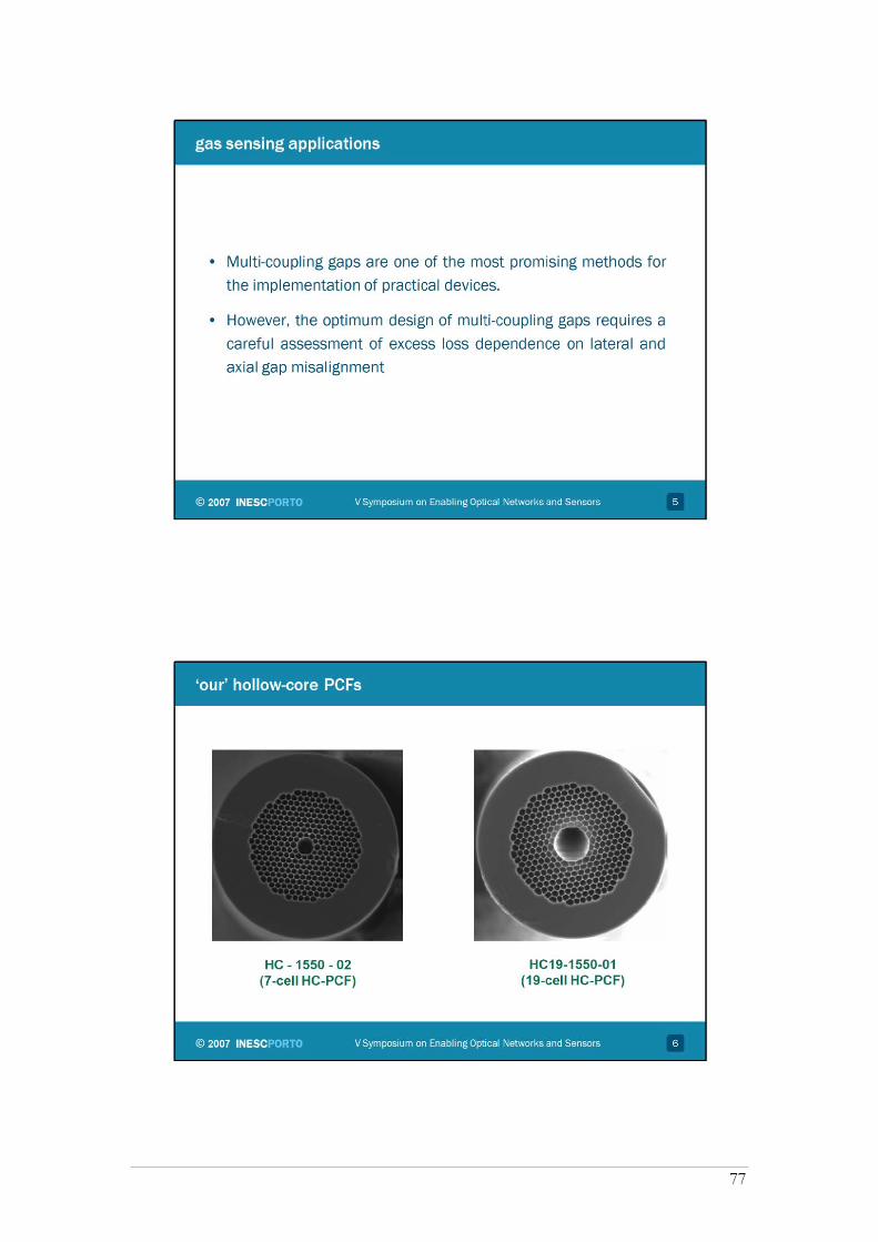
77

78
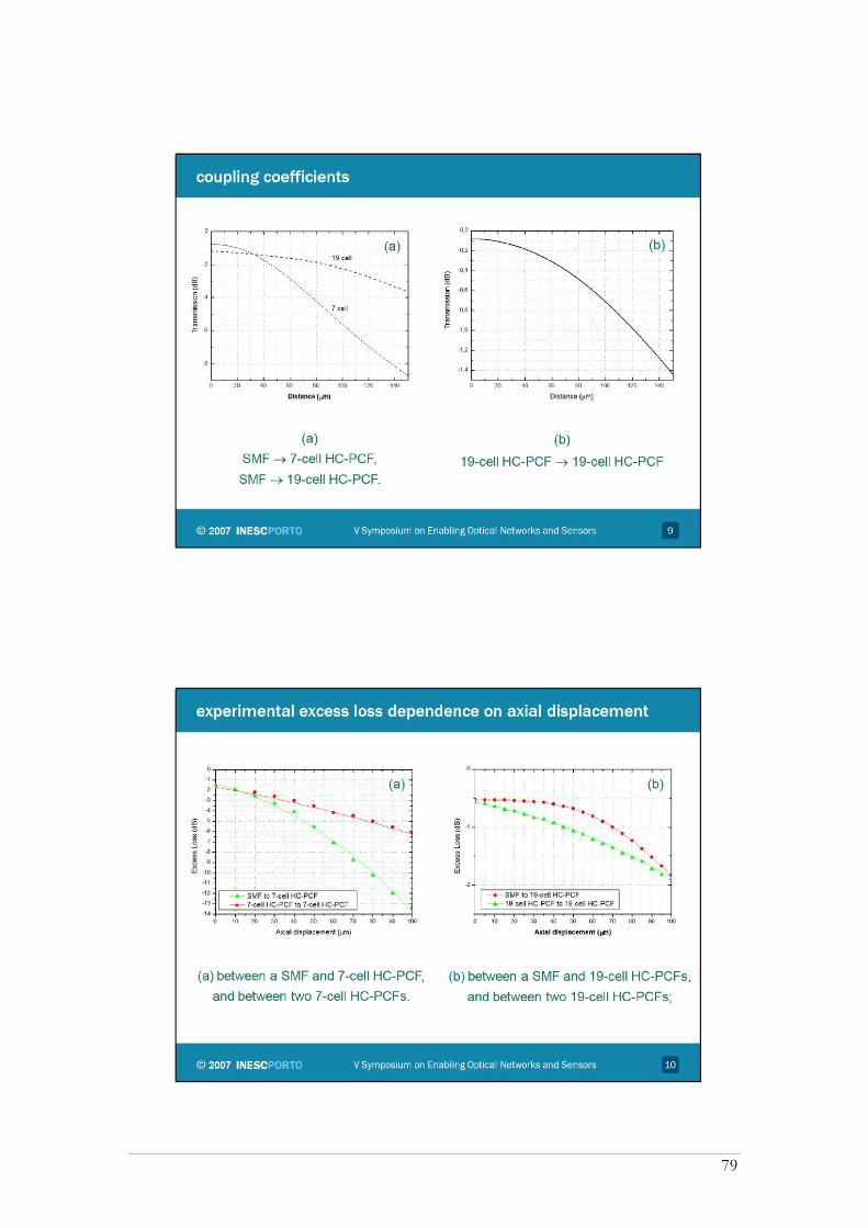
79

80

81

82
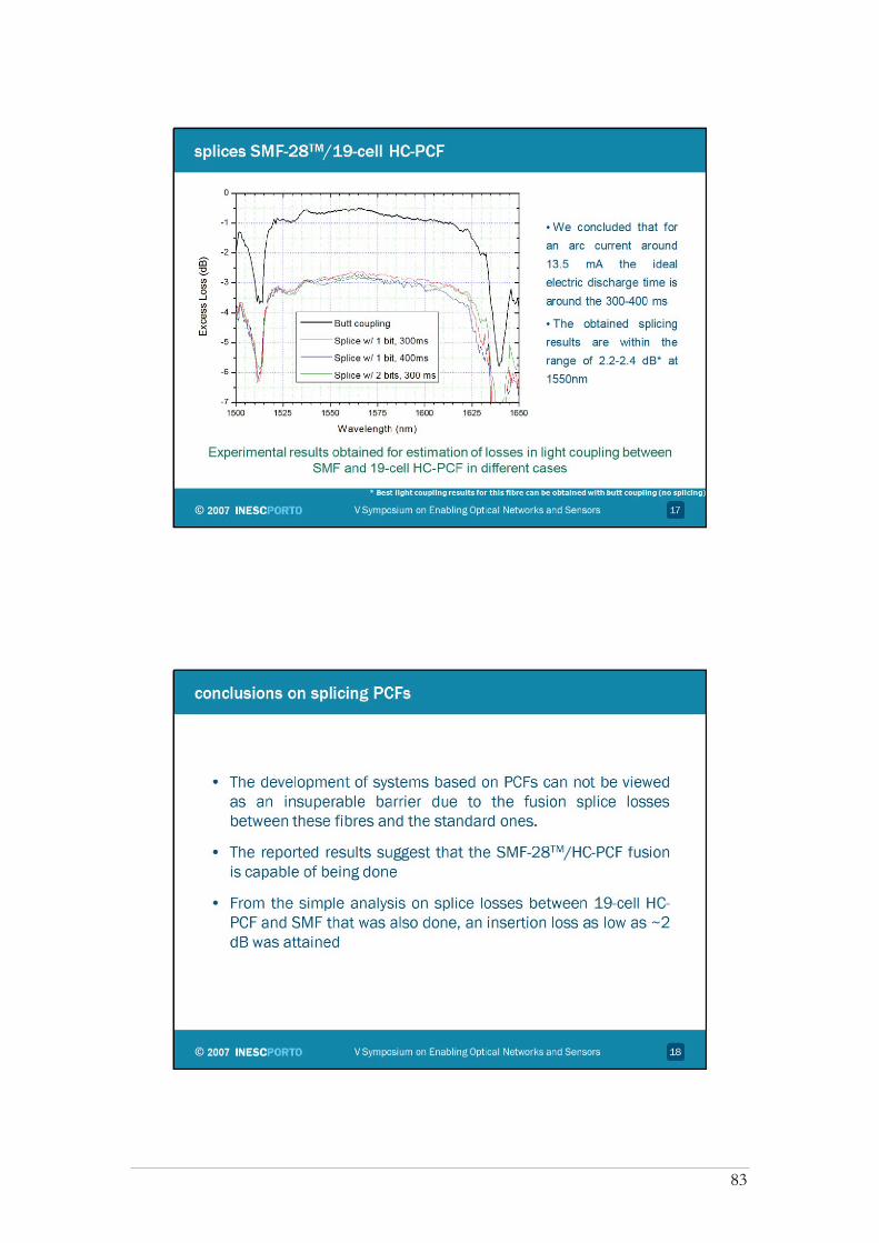
83

84
11 References 1. Michaels, P.J., et al. Methane Matters. 2007 [cited; Available from:
http://www.worldclimatereport.com/index.php/2007/04/13/methane-matters/. 2. Moore, C.B., Gas-Laser Frequency Selection by Molecular Absorption.
Applied Optics, 1965. 4(2): p. 252-253. 3. Grant, W.B., He-Ne and CW CO2-Laser Long-Path Systems for Gas-
Detection. Applied Optics, 1986. 25(5): p. 709-719. 4. Uehara, K. and H. Tai, Remote Detection of Methane with a 1.66-Mu-M
Diode-Laser. Applied Optics, 1992. 31(6): p. 809-814. 5. Silveira, J.P. and F. Grasdepot, CH4 Optical Sensor Using a 1.31 Mu-M DFB
Laser-Diode. Sensors and Actuators B-Chemical, 1995. 25(1-3): p. 603-606. 6. Stewart, G., et al., Interferometric signals in fiber optic methane sensors with
wavelength modulation of the DFB laser source. Lightwave Technology, Journal of, 1998. 16(1): p. 43-53.
7. Iseki, T., H. Tai, and K. Kimura, A portable remote methane sensor using a tunable diode laser. Measurement Science and Technology, 2000. 11: p. 594-602.
8. Chan, K., H. Ito, and H. Inaba, Remote sensing system for near-infrared differential absorption of CH4 gas using low-loss optical fiber link. Appl. Opt., 1984. 23(19): p. 3415-3419.
9. Chan, K., et al., 10 Km-Long Fibre-Optic Remote-Sensing of CH4 Gas by near-Infrared Absorption. Applied Physics B-Photophysics and Laser Chemistry, 1985. 38(1): p. 11-15.
10. Whitenett, G., et al., Optical fibre instrumentation for environmental monitoring applications. Journal of Optics a-Pure and Applied Optics, 2003. 5(5): p. S140-S145.
11. Kosterev, A.A., Y.A. Bakhirkin, and F.K. Tittel, Ultrasensitive gas detection by quartz-enhanced photoacoustic spectroscopy in the fundamental molecular absorption bands region. Applied Physics B: Lasers and Optics, 2005. 80(1): p. 133-138.
12. Culshaw, B., et al., Evanescent Wave Methane Detection Using Optical Fibers. Electronics Letters, 1992. 28(24): p. 2232-2234.
13. Stewart, G., W. Jin, and B. Culshaw, Prospects for fibre-optic evanescent-field gas sensors using absorption in the near-infrared. Sensors and Actuators B: Chemical, 1997. 38(1-3): p. 42-47.
14. Muhammad, F.A., et al., Sensitivity enhancement of D-fibre methane gas sensor using high-index overlay. Optoelectronics [see also IEEE Proceedings-Optoelectronics], IEEE Proceedings J, 1993. 140(2): p. 115-118.
15. Benounis, M., et al., Study of a new evanescent wave optical fibre sensor for methane detection based on cryptophane molecules. Sensors and Actuators B-Chemical, 2005. 107(1): p. 32-39.
16. Roy, R.K., M.P. Chowdhury, and A.K. Pal, Room temperature sensor based on carbon nanotubes and nanofibres for methane detection. Vacuum, 2005. 77(3): p. 223-229.
17. Fini, J.M., Microstructure fibres for optical sensing in gases and liquids. Measurement Science and Technology, 2004. 15(6): p. 1120-1128.
18. Monro, T.M., et al., Sensing with microstructured optical fibres. Measurement Science and Technology, 2001. 12: p. 854-858.
85

19. Cregan, R.F., et al., Single-mode photonic band gap guidance of light in air. Science, 1999. 285(5433): p. 1537-1539.
20. Ritari, T., et al., Gas sensing using air-guiding photonic bandgap fibers. Opt. Express, 2004. 12(17): p. 4080-4087.
21. Cubillas, A.M., et al. High sensitive Methane Sensor based on a Photonic Bandgap Fiber. in EWOFS 2007. 2007. Napoli.
22. Cubillas, A.M., et al., Methane detection at 1670-nm band using a hollow-core photonic bandgap fiber and a multiline algorithm. Opt. Express, 2007. 15(26): p. 17570-17576.
23. Noda, K., et al., Measurement of methane gas concentration by detecting absorption at 1300 nm using a laser diode wavelength-sweep technique. Optical Engineering, 2005. 44(1): p. 014301-6.
24. Russell, P., Photonic Crystal Fibers. Science, 2003. 299(5605): p. 358-362. 25. BlazePhotonics. Photonic Crystal Fibers. 2004 [cited; Available from:
http://www.blazephotonics.com. 26. Thorlabs, Tools of the trade. 2007. 19: p. 1080-1084. 27. Knight, J.C., Photonic crystal fibres. Nature, 2003. 424(6950): p. 847-851. 28. Nielsen, M.D., et al., Low-loss photonic crystal fibers for transmission systems
and their dispersion properties. Optics Express, 2004. 12(7): p. 1372-1376. 29. Mangan, B.J., et al. Low loss (1.7 dB/km) hollow core photonic bandgap fiber.
in Optical Fiber Communication Conference, 2004. OFC 2004. 2004. 30. Ferreira, L.A., Interrogação de Sensores de Bragg em Fibra Óptica, in FCUP
- Departamento de Física. 1999, Universidade do Porto. 31. Bisbee, D.L., Splicing silica fibers with an electric arc. Appl. Opt., 1976.
15(3): p. 796-798. 32. Bourliaguet, B., et al., Microstructured fiber splicing. Opt. Express, 2003.
11(25): p. 3412-3417. 33. Chong, J.H. and M. Rao, Development of a system for laser splicing photonic
crystal fiber. Opt. Express, 2003. 11(12): p. 1365-1370. 34. O. Frazão, J.P.C., H. M. Salgado, Low-loss splice in a microstructured fibre
using a conventional fusion splicer. Microwave and Optical Tech Lett 2005. 46(2): p. 172-174.
35. Lizier, J.T. and G.E. Town, Splice losses in holey optical fibers. Photonics Technology Letters, IEEE, 2001. 13(8): p. 794-796.
36. Avanex. PowerSourceΤΜ 1905 LMI. 2005 [cited; Available from: http://www.ilxlightwave.com/laser-diode/Data/1905lmc.pdf.
37. Hoo, Y.L., et al., Evanescent-wave gas sensing using microstructure fiber. Optical Engineering, 2002. 41(1): p. 8-9.
38. Monro, T.M., D.J. Richardson, and P.J. Bennett, Developing holey fibres for evanescent field devices. Electronics Letters, 1999. 35(14): p. 1188-1189.
39. Hoo, Y.L., et al., Design and Modeling of a Photonic Crystal Fiber Gas Sensor. Appl. Opt., 2003. 42(18): p. 3509-3515.
40. Lide, D.R., Handbook of Chemistry and Physics. 78th ed. 1997-1998: CRC Press.
41. Hoo, Y.L., et al., Measurement of gas diffusion coefficient using photonic crystal fiber. Photonics Technology Letters, IEEE, 2003. 15(10): p. 1434-1436.
86