Embed Size (px)
Citation preview
Development of Freeway Operational Strategies with
IRIS-in-Loop Simulation
Eil Kwon, Principal InvestigatorDepartment of Civil EngineeringUniversity of Minnesota Duluth
Northland Advanced Transportation Systems Research Laboratory
University of Minnesota Duluth
January 2012Research Project
Final Report 2012-04

All agencies, departments, divisions and units that develop, use and/or purchase written materials for distribution to the public must ensure that each document contain a statement indicating that the information is available in alternative formats to individuals with disabilities upon request. Include the following statement on each document that is distributed: To request this document in an alternative format, call Bruce Lattu at 651-366-4718 or 1-800-657-3774 (Greater Minnesota); 711 or 1-800-627-3529 (Minnesota Relay). You may also send an e-mail to [email protected]. (Please request at least one week in advance).
Technical Report Documentation Page 1. Report No. 2. 3. Recipients Accession No. MN/RC 2012-04 4. Title and Subtitle 5. Report Date
Development of Freeway Operational Strategies with IRIS-in-Loop Simulation
January 2012 6.
7. Author(s) 8. Performing Organization Report No. Eil Kwon and Chongmyung Park 9. Performing Organization Name and Address 10. Project/Task/Work Unit No. Department of Civil Engineering Northland Advanced Transportation Systems Research Laboratory University of Minnesota Duluth 1405 University Drive Duluth, MN 55812
CTS Project #2010020 11. Contract (C) or Grant (G) No.
(c) 89261 (wo) 169
12. Sponsoring Organization Name and Address 13. Type of Report and Period Covered Minnesota Department of Transportation Research Services Section 395 John Ireland Boulevard Mail Stop 330 St. Paul, Minnesota 55155
Final Report 14. Sponsoring Agency Code
15. Supplementary Notes http://www.lrrb.org/pdf/201204.pdf 16. Abstract (Limit: 250 words) This research produced several important tools that are essential in managing and operating freeway corridors. First, a computer-based off-line process was developed to automatically estimate a set of traffic measures for a given freeway corridor using the historical detector data. Secondly, a prototype on-line estimation procedure was designed to calculate selected traffic measures in real time to assist operators in identifying abnormal traffic patterns. Third, the IRIS-in-loop simulation system was developed by linking IRIS, the freeway control system developed by MnDOT, to a microscopic simulation software through a data communication module, so that new operational strategies can be directly coded into IRIS and evaluated under the realistic simulation environment. Finally, two new freeway operational strategies, variable speed limit control and a density-based adaptive ramp metering strategy, were developed and evaluated with the IRSI-in-Loop simulation system.
17. Document Analysis/Descriptors Freeway traffic measures, Simulation, Freeway management systems, Variable speed limit control, Speed control, Ramp metering
18. Availability Statement No restrictions. Document available from: National Technical Information Services, Alexandria, Virginia 22312
19. Security Class (this report) 20. Security Class (this page) 21. No. of Pages 22. Price Unclassified Unclassified 79
Development of Freeway Operational Strategies with IRIS-in-Loop Simulation
Final Report
Prepared by:
Eil Kwon Chongmyung Park
Department of Civil Engineering
Northland Advanced Transportation Systems Research Laboratory University of Minnesota Duluth
January 2012
Published by:
Minnesota Department of Transportation Research Services Section
395 John Ireland Boulevard, Mail Stop 330 St. Paul, Minnesota 55155
This report represents the results of research conducted by the authors and does not necessarily represent the views or policies of the Minnesota Department of Transportation or the University of Minnesota Duluth. This report does not contain a standard or specified technique. The authors, the Minnesota Department of Transportation, and the University of Minnesota Duluth do not endorse products or manufacturers. Any trade or manufacturers’ names that may appear herein do so solely because they are considered essential to this report.

ACKNOWLEDGMENTS
This research was financially supported by the Minnesota Department of Transportation. The authors greatly appreciate the technical guidance and data support from the engineers at the Regional Transportation Management Center, in particular, Brian Kary, Doug Lau and Jesse Larson. Also, the administrative support from Dan Warzala is very much appreciated.
TABLE OF CONTENTS
1 INTRODUCTION ................................................................................................................... 1
1.1 Background and Research Objectives .............................................................................. 1
1.2 Report Organization ......................................................................................................... 1
2 DEVELOPMENT OF THE IRIS-IN-LOOP SIMULATION SYSTEM ................................ 2
2.1 Structure of IRIS-in-Loop Simulation System................................................................. 2
2.2 Communicator .................................................................................................................. 4
2.3 Data Manager ................................................................................................................. 13
2.4 VISSIM Controller ......................................................................................................... 16
3 DEVELOPMENT OF AN OFF-LINE ESTIMATION PROCESS FOR FREEWAY TRAFFIC CONDITIONS ............................................................................................................. 20
3.1 Structure of Traffic Information and Condition Analysis System (TICAS) .................. 20
3.2 Traffic Condition Measures in TICAS ........................................................................... 23
3.3 Data Structure of TICAS ................................................................................................ 24
4 DEVELOPMENT OF AN ON-LINE ESTIMATION PROCESS FOR FREEWAY TRAFFIC CONDITIONS ............................................................................................................. 31
4.1 Data Structure and Operational Sequence of On-Line Process ...................................... 31
4.2 Example On-Line Graphs for Selected Traffic Parameters ........................................... 35
5 MICROSCOPIC MODELING A FREEWAY CORRIDOR FOR EXAMPLE APPLICATION OF ILSS WITH FREEWAY OPERATIONAL STRATEGIES ....................... 38
5.1 Sample Freeway Corridor .............................................................................................. 38
5.2 Modeling and Calibration of Vissim for Sample Freeway Corridor .............................. 39
6 DEVELOPMENT AND EVALUATION OF VARIABLE SPEED LIMIT CONTROL STRATEGY .................................................................................................................................. 42
6.1 Overview of the Variable Speed Limit Control Approach ............................................ 42
6.2 Identification of VSL Starting Locations ....................................................................... 44
6.3 Determination of Speed Control Zones and Advisory Speed Limits ............................. 45
6.4 Assessment of VSL Control Strategy with Microscopic Simulation ............................. 46
7 DEVELOPMENT AND TESTING OF NEW RAMP METERING ALGORITHM ........... 48
7.1 Overview of New Ramp Metering Strategy ................................................................... 48
7.2 Identification of Bottlenecks .......................................................................................... 49
7.3 Determination of Metering Rates for Entrance Ramps Controlled by Each Bottleneck 50
7.4 Incorporation of the New Algorithm into IRIS .............................................................. 56
7.5 Evaluation of the New Algorithm using IRIS-in-Loop Simulation System .................. 57
8 CONCLUSIONS ................................................................................................................... 61

REFERENCES ............................................................................................................................. 63
APPENDIX A. PROCESS TO INCORPORATE NEW METERING ALGORITHM INTO IRIS
APPENDIX B. SPEED CONTOURS FROM SIMULATION RESULTS
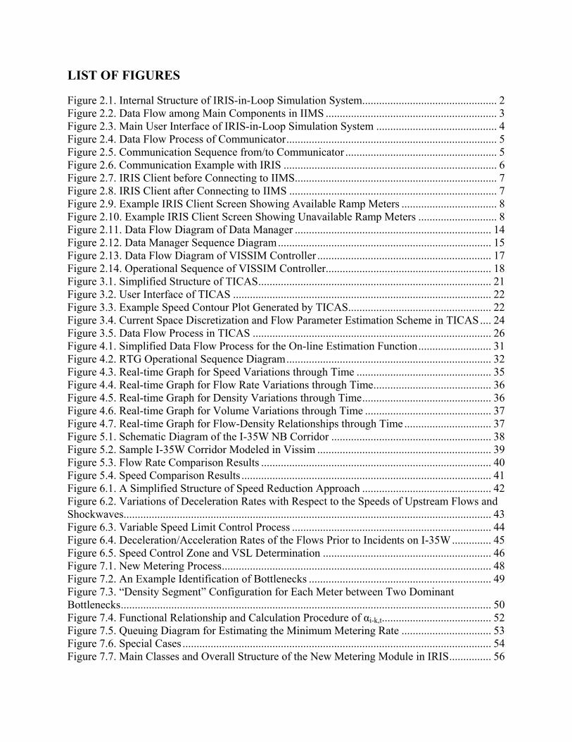
LIST OF FIGURES
Figure 2.1. Internal Structure of IRIS-in-Loop Simulation System................................................ 2 Figure 2.2. Data Flow among Main Components in IIMS ............................................................. 3 Figure 2.3. Main User Interface of IRIS-in-Loop Simulation System ........................................... 4 Figure 2.4. Data Flow Process of Communicator ........................................................................... 5 Figure 2.5. Communication Sequence from/to Communicator ...................................................... 5 Figure 2.6. Communication Example with IRIS ............................................................................ 6 Figure 2.7. IRIS Client before Connecting to IIMS ........................................................................ 7 Figure 2.8. IRIS Client after Connecting to IIMS .......................................................................... 7 Figure 2.9. Example IRIS Client Screen Showing Available Ramp Meters .................................. 8 Figure 2.10. Example IRIS Client Screen Showing Unavailable Ramp Meters ............................ 8 Figure 2.11. Data Flow Diagram of Data Manager ...................................................................... 14 Figure 2.12. Data Manager Sequence Diagram ............................................................................ 15 Figure 2.13. Data Flow Diagram of VISSIM Controller .............................................................. 17 Figure 2.14. Operational Sequence of VISSIM Controller ........................................................... 18 Figure 3.1. Simplified Structure of TICAS ................................................................................... 21 Figure 3.2. User Interface of TICAS ............................................................................................ 22 Figure 3.3. Example Speed Contour Plot Generated by TICAS ................................................... 22 Figure 3.4. Current Space Discretization and Flow Parameter Estimation Scheme in TICAS .... 24 Figure 3.5. Data Flow Process in TICAS ..................................................................................... 26 Figure 4.1. Simplified Data Flow Process for the On-line Estimation Function .......................... 31 Figure 4.2. RTG Operational Sequence Diagram ......................................................................... 32 Figure 4.3. Real-time Graph for Speed Variations through Time ................................................ 35 Figure 4.4. Real-time Graph for Flow Rate Variations through Time .......................................... 36 Figure 4.5. Real-time Graph for Density Variations through Time .............................................. 36 Figure 4.6. Real-time Graph for Volume Variations through Time ............................................. 37 Figure 4.7. Real-time Graph for Flow-Density Relationships through Time ............................... 37 Figure 5.1. Schematic Diagram of the I-35W NB Corridor ......................................................... 38 Figure 5.2. Sample I-35W Corridor Modeled in Vissim .............................................................. 39 Figure 5.3. Flow Rate Comparison Results .................................................................................. 40 Figure 5.4. Speed Comparison Results ......................................................................................... 41 Figure 6.1. A Simplified Structure of Speed Reduction Approach .............................................. 42 Figure 6.2. Variations of Deceleration Rates with Respect to the Speeds of Upstream Flows and Shockwaves................................................................................................................................... 43 Figure 6.3. Variable Speed Limit Control Process ....................................................................... 44 Figure 6.4. Deceleration/Acceleration Rates of the Flows Prior to Incidents on I-35W .............. 45 Figure 6.5. Speed Control Zone and VSL Determination ............................................................ 46 Figure 7.1. New Metering Process ................................................................................................ 48 Figure 7.2. An Example Identification of Bottlenecks ................................................................. 49 Figure 7.3. “Density Segment” Configuration for Each Meter between Two Dominant Bottlenecks .................................................................................................................................... 50 Figure 7.4. Functional Relationship and Calculation Procedure of αi-k,t ....................................... 52 Figure 7.5. Queuing Diagram for Estimating the Minimum Metering Rate ................................ 53 Figure 7.6. Special Cases .............................................................................................................. 54 Figure 7.7. Main Classes and Overall Structure of the New Metering Module in IRIS ............... 56

Figure 7.8. I-35W NB in Vissim ................................................................................................... 57 Figure 7.9. 169 SB in Vissim ........................................................................................................ 58

LIST OF TABLES
Table 6.1. VSL Evaluation Results with Normal Traffic Flows (for a 3-hour Peak Period) ........ 47 Table 6.2. VSL Evaluation Results with an Incident (for a 3-hour Peak Period) ......................... 47 Table 7.1. Summary Simulation Results with I-35W NB Test Section ........................................ 59 Table 7.2. Summary Simulation Results with 169 SB Test Section ............................................. 60
EXECUTIVE SUMMARY
Developing efficient and robust traffic operational strategies that can directly be implemented into the existing working environment is of critical importance in improving the efficiency and the effectiveness of freeway management. This research produced several important tools that are essential in achieving such an efficient freeway operations. First, a computer-based off-line process was developed to automatically estimate a set of traffic measures for a given freeway corridor for selected time periods using the historical data collected from the field detectors. Secondly, a prototype on-line process was developed to calculate and graphically present selected traffic measures in real time to assist the traffic operators in identifying abnormal flow patterns. Third, an integrated simulation system was developed by combining IRIS, the freeway traffic control system developed by MnDOT, and the Vissim microscopic simulation software, so that new operational strategies can be directly coded into IRIS and evaluated under the realistic simulation environment. The resulting IRIS-in-Loop Simulation System (ILSS) makes it possible to develop the operational strategies that can directly work under the current freeway operational environment. In this research, the ILSS was applied to assess the performance of two new operational strategies that were also developed in this study: Variable Advisory Speed Limit Control and Density-based Adaptive Metering Strategies. The new variable advisory speed limit control strategy is designed to mitigate the shock waves propagated from downstream bottlenecks by gradually reducing the speed levels of the incoming traffic flows. The algorithm first identifies the locations of the bottlenecks and the VSL control zones by examining the flow deceleration rates between two detector stations in a given corridor. The advisory speed limits for each control zone are calculated with a constant deceleration rate, which has been determined to result in minimum increases in travel times. The preliminary evaluation results with microscopic simulation indicate that the proposed VSL system could significantly reduce the sudden deceleration rates of the traffic flows reacting to fixed or moving bottlenecks, while the increases in travel times can be kept relatively small. The variable speed limit control strategy has been implemented at the I-35W corridor in July 2010 and the detailed analysis of the field data will be conducted in a subsequent phase of this research. Finally, an adaptive ramp metering strategy based on traffic density was developed and evaluated with ILSS. The new algorithm identifies bottlenecks for a given corridor every 30 seconds and determines the metering rates for each entrance ramp with the estimated mainline ‘segment density’. Further, the ramp wait time restriction is explicitly incorporated into the metering rate calculation. The new algorithm was evaluated with ILSS using two freeway corridors as the sample test sections. The simulation analysis with ILSS indicates that the new algorithm can significantly reduce the amount of congestion, compared to the existing metering method, while handling similar level of traffic flows. Future research needs include the field testing of the proposed ramp metering strategy, enhancement of the variable speed limit control algorithm to manage different weather conditions, and development of predictive control strategies for proactive traffic management.
1
1 INTRODUCTION
1.1 Background and Research Objectives
Developing efficient and robust traffic operational strategies that can directly be implemented into the existing working environment is of critical importance in improving the effectiveness of freeway management. Currently the freeway network in the Twin Cites is being managed with the Intelligent Road Information System (IRIS), a computerized operating system developed by the Minnesota Department of Transportation (MnDOT) to operate field devices such as ramp meters, variable message signs and loop detectors (MnDOT, 2008). This research develops a comprehensive support tool for IRIS by integrating it with a microscopic traffic simulator, so that the IRIS-based freeway operational strategies can be emulated and refined in the simulated environment prior to field implementation. The resulting IRIS-in-Loop Simulation system (ILSS) will be applied to develop new freeway operational strategies, including variable speed limit control and density-based adaptive ramp metering algorithms. Further, a computerized off/on-line process will be developed to estimate a set of the traffic performance measures for given corridors during selected periods. The resulting off-line performance measures will be used to support different levels of decision making process at MnDOT in planning and operations of the freeway network, including the continuous refinements ramp metering, incident management and travel time information systems, while the on-line measures for traffic conditions can be used for expanding the driver information system. Finally new operational strategies for freeway corridors will be developed and evaluated with ILSS. First, a variable speed limit control strategy will be developed to mitigate the rapid propagation of shock waves, so that the possibility of rear-end collision can be reduced. Also, an alternative ramp metering algorithm will be developed to address the issues with the current capacity-based zone control approach (Kwon, et. al., 2005, Kwon, et. al, 2001). The new metering algorithm will also be tested with ILSS using real freeway corridors.
1.2 Report Organization
Chapter 2 develops an integrated simulation environment by combining IRIS and a microscopic simulator through a data conversion module. In Chapter 3, an off-line process is developed to automatically estimate a set of traffic performance measures for selected freeway sections for a given time period. Computer software is also developed to automate the process. Chapter 4 summarizes the on-line estimation process for a selected set of traffic measures that can be used to support real-time operations. In Chapter 5, a microscopic simulation software is used to model a section of freeway, which is used as the test section to evaluate the performance of the new freeway operational strategies to be developed in the subsequent chapters. In Chapter 6, a new variable speed limit control strategy is developed and tested in a simulation environment. An alternative ramp metering strategy based on traffic density measures is also developed and tested in Chapter 7. Finally Chapter 8 summarizes the findings of this research and identifies further research needs.
2
2 DEVELOPMENT OF THE IRIS-IN-LOOP SIMULATION SYSTEM
2.1 Structure of IRIS-in-Loop Simulation System
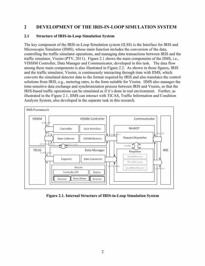
The key component of the IRIS-in-Loop Simulation system (ILSS) is the Interface for IRIS and Microscopic Simulator (IIMS), whose main function includes the conversion of the data, controlling the traffic simulator operations, and managing data transactions between IRIS and the traffic simulator, Vissim (PTV, 2011). Figure 2.1 shows the main components of the IIMS, i.e., VISSIM Controller, Data Manager and Communicator, developed in this task. The data flow among these main components is also illustrated in Figure 2.2. As shown in those figures, IRIS and the traffic simulator, Vissim, is continuously interacting through time with IIMS, which converts the simulated detector data to the format required by IRIS and also translates the control solutions from IRIS, e.g., metering rates, to the form suitable for Vissim. IIMS also manages the time-sensitive data exchange and synchronization process between IRIS and Vissim, so that the IRIS-based traffic operations can be simulated as if it’s done in real environment. Further, as illustrated in the Figure 2.1, IIMS can interact with TICAS, Traffic Information and Condition Analysis System, also developed in the separate task in this research.
Figure 2.1. Internal Structure of IRIS-in-Loop Simulation System
3
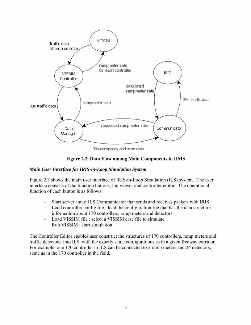
Figure 2.2. Data Flow among Main Components in IIMS
Main User Interface for IRIS-in-Loop Simulation System
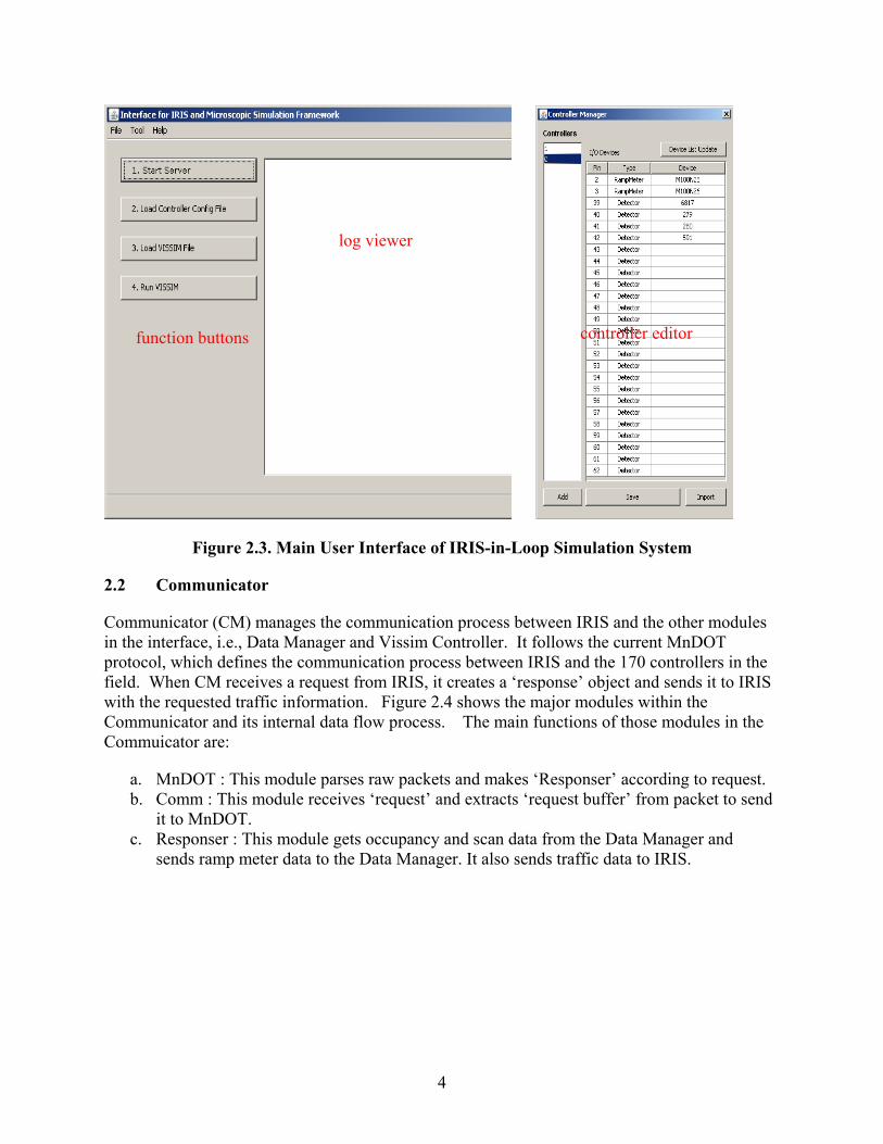
Figure 2.3 shows the main user interface of IRIS-in-Loop Simulation (ILS) system. The user interface consists of the function buttons, log viewer and controller editor. The operational function of each button is as follows:
- Start server : start ILS Communicator that sends and receives packets with IRIS - Load controller config file : load the configuration file that has the data structure
information about 170 controllers, ramp meters and detectors - Load VISSIM file : select a VISSIM case file to simulate - Run VISSIM : start simulation
The Controller Editor enables user construct the structures of 170 controllers, ramp meters and traffic detectors into ILS with the exactly same configurations as in a given freeway corridor. For example, one 170 controller in ILS can be connected to 2 ramp meters and 24 detectors, same as in the 170 controller in the field.
4
Figure 2.3. Main User Interface of IRIS-in-Loop Simulation System
2.2 Communicator
Communicator (CM) manages the communication process between IRIS and the other modules in the interface, i.e., Data Manager and Vissim Controller. It follows the current MnDOT protocol, which defines the communication process between IRIS and the 170 controllers in the field. When CM receives a request from IRIS, it creates a ‘response’ object and sends it to IRIS with the requested traffic information. Figure 2.4 shows the major modules within the Communicator and its internal data flow process. The main functions of those modules in the Commuicator are:
a. MnDOT : This module parses raw packets and makes ‘Responser’ according to request. b. Comm : This module receives ‘request’ and extracts ‘request buffer’ from packet to send
it to MnDOT. c. Responser : This module gets occupancy and scan data from the Data Manager and
sends ramp meter data to the Data Manager. It also sends traffic data to IRIS.
log viewer
function buttons controller editor
5
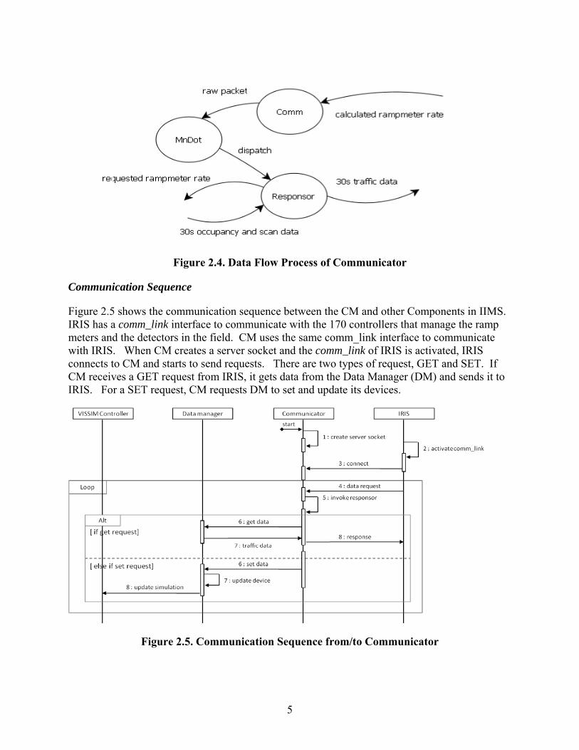
Figure 2.4. Data Flow Process of Communicator
Communication Sequence
Figure 2.5 shows the communication sequence between the CM and other Components in IIMS. IRIS has a comm_link interface to communicate with the 170 controllers that manage the ramp meters and the detectors in the field. CM uses the same comm_link interface to communicate with IRIS. When CM creates a server socket and the comm_link of IRIS is activated, IRIS connects to CM and starts to send requests. There are two types of request, GET and SET. If CM receives a GET request from IRIS, it gets data from the Data Manager (DM) and sends it to IRIS. For a SET request, CM requests DM to set and update its devices.
Figure 2.5. Communication Sequence from/to Communicator
6
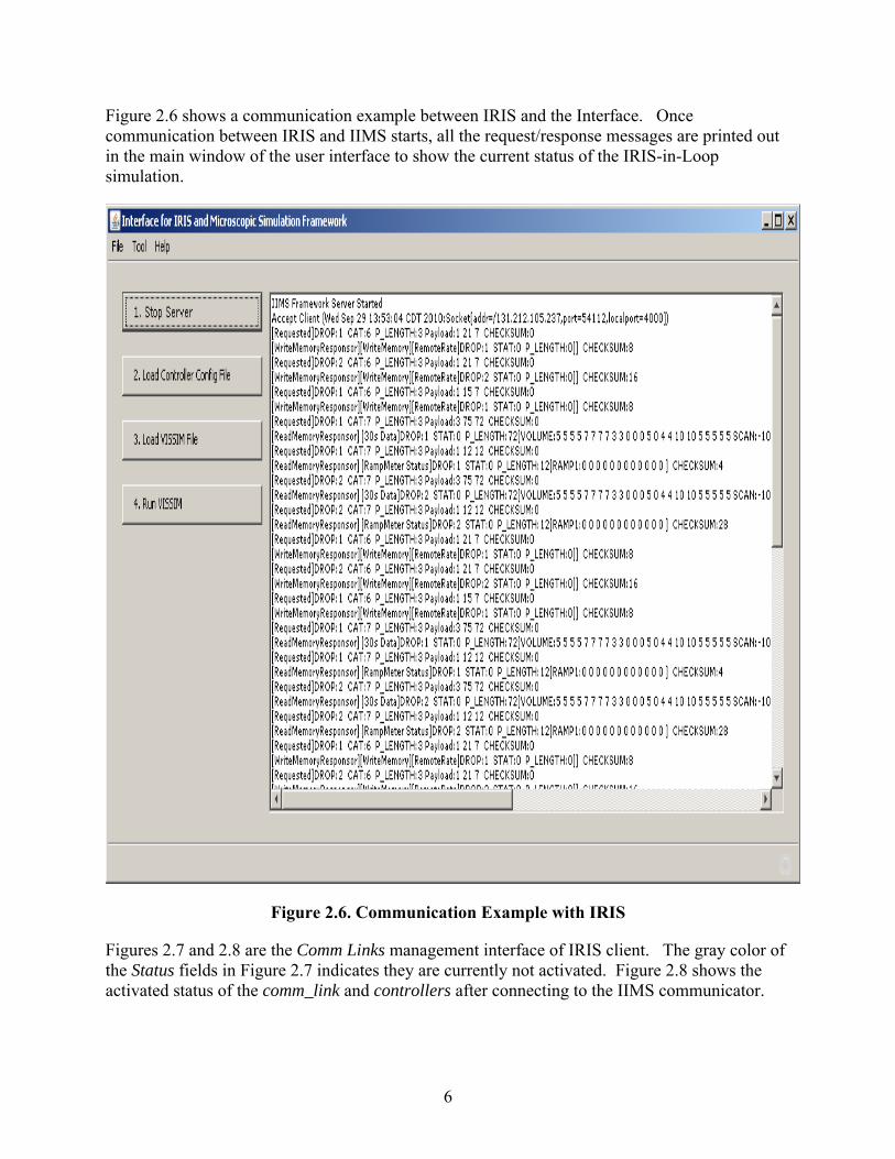
Figure 2.6 shows a communication example between IRIS and the Interface. Once communication between IRIS and IIMS starts, all the request/response messages are printed out in the main window of the user interface to show the current status of the IRIS-in-Loop simulation.
Figure 2.6. Communication Example with IRIS
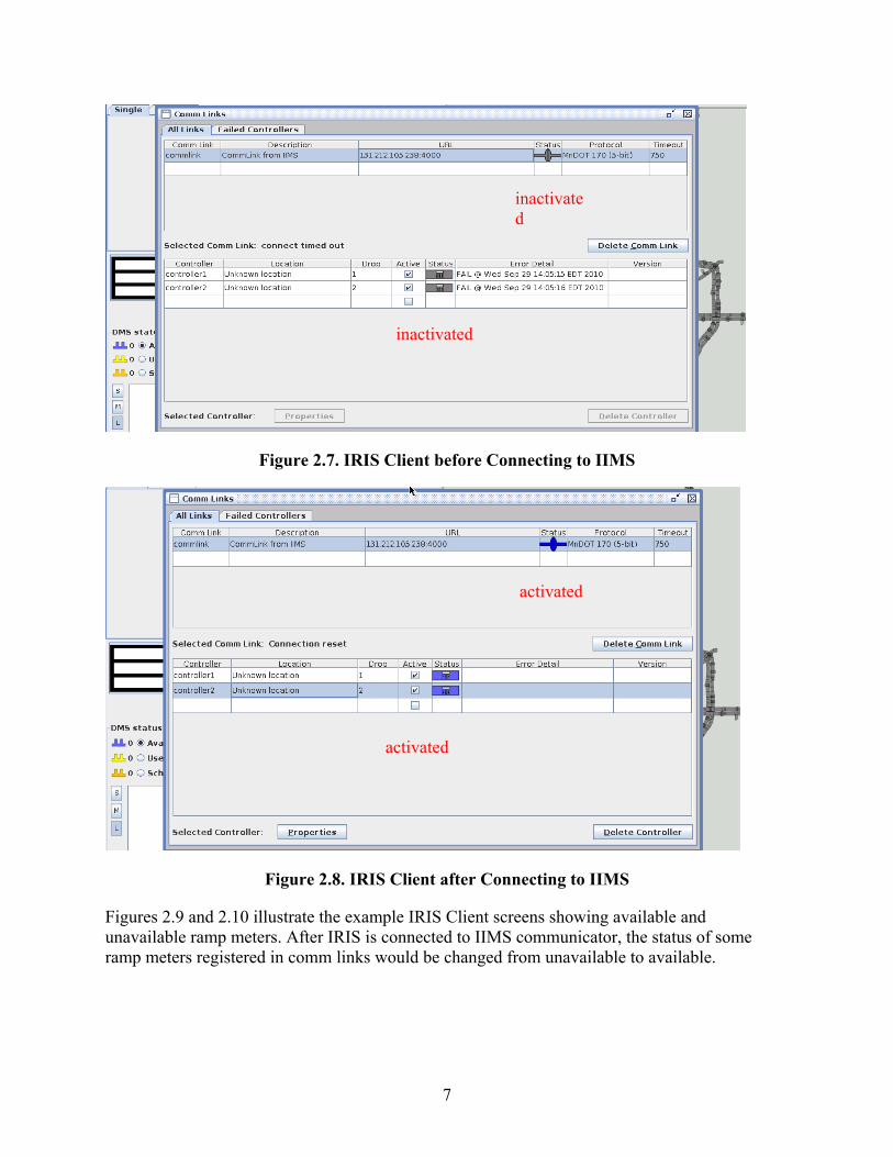
Figures 2.7 and 2.8 are the Comm Links management interface of IRIS client. The gray color of the Status fields in Figure 2.7 indicates they are currently not activated. Figure 2.8 shows the activated status of the comm_link and controllers after connecting to the IIMS communicator.
7
inactivated
inactivated
Figure 2.7. IRIS Client before Connecting to IIMS
activated
activated
Figure 2.8. IRIS Client after Connecting to IIMS
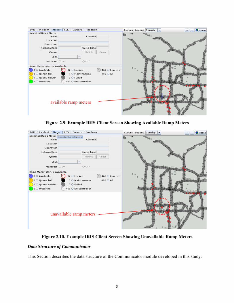
Figures 2.9 and 2.10 illustrate the example IRIS Client screens showing available and unavailable ramp meters. After IRIS is connected to IIMS communicator, the status of some ramp meters registered in comm links would be changed from unavailable to available.
8
Figure 2.9. Example IRIS Client Screen Showing Available Ramp Meters
Figure 2.10. Example IRIS Client Screen Showing Unavailable Ramp Meters
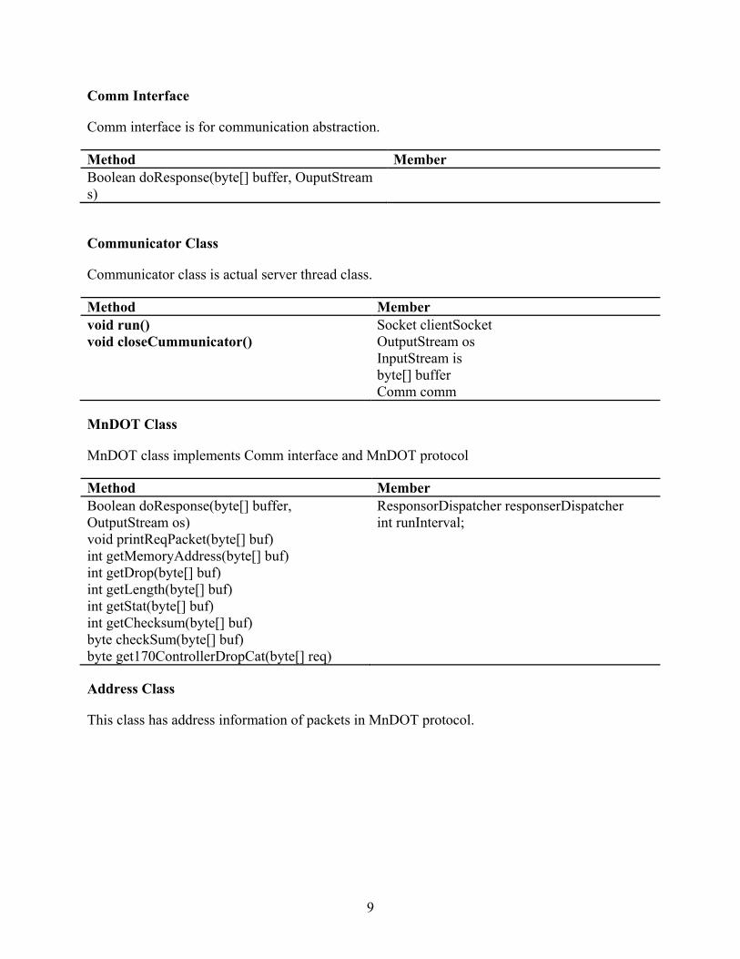
Data Structure of Communicator
This Section describes the data structure of the Communicator module developed in this study.
available ramp meters
unavailable ramp meters
9
Comm Interface
Comm interface is for communication abstraction.
Method Member Boolean doResponse(byte[] buffer, OuputStream s)
Communicator Class
Communicator class is actual server thread class.
Method Member void run() void closeCummunicator()
Socket clientSocket OutputStream os InputStream is byte[] buffer Comm comm
MnDOT Class
MnDOT class implements Comm interface and MnDOT protocol
Method Member Boolean doResponse(byte[] buffer, OutputStream os) void printReqPacket(byte[] buf) int getMemoryAddress(byte[] buf) int getDrop(byte[] buf) int getLength(byte[] buf) int getStat(byte[] buf) int getChecksum(byte[] buf) byte checkSum(byte[] buf) byte get170ControllerDropCat(byte[] req)
ResponsorDispatcher responserDispatcher int runInterval;
Address Class
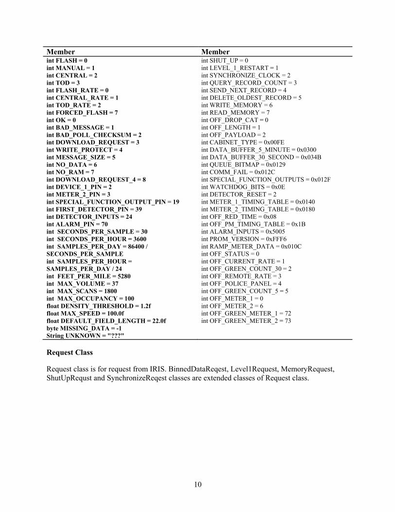
This class has address information of packets in MnDOT protocol.
10
Member Member int FLASH = 0 int MANUAL = 1 int CENTRAL = 2 int TOD = 3 int FLASH_RATE = 0 int CENTRAL_RATE = 1 int TOD_RATE = 2 int FORCED_FLASH = 7 int OK = 0 int BAD_MESSAGE = 1 int BAD_POLL_CHECKSUM = 2 int DOWNLOAD_REQUEST = 3 int WRITE_PROTECT = 4 int MESSAGE_SIZE = 5 int NO_DATA = 6 int NO_RAM = 7 int DOWNLOAD_REQUEST_4 = 8 int DEVICE_1_PIN = 2 int METER_2_PIN = 3 int SPECIAL_FUNCTION_OUTPUT_PIN = 19 int FIRST_DETECTOR_PIN = 39 int DETECTOR_INPUTS = 24 int ALARM_PIN = 70 int SECONDS_PER_SAMPLE = 30 int SECONDS_PER_HOUR = 3600 int SAMPLES_PER_DAY = 86400 / SECONDS_PER_SAMPLE int SAMPLES_PER_HOUR = SAMPLES_PER_DAY / 24 int FEET_PER_MILE = 5280 int MAX_VOLUME = 37 int MAX_SCANS = 1800 int MAX_OCCUPANCY = 100 float DENSITY_THRESHOLD = 1.2f float MAX_SPEED = 100.0f float DEFAULT_FIELD_LENGTH = 22.0f byte MISSING_DATA = -1 String UNKNOWN = "???"
int SHUT_UP = 0 int LEVEL_1_RESTART = 1 int SYNCHRONIZE_CLOCK = 2 int QUERY_RECORD_COUNT = 3 int SEND_NEXT_RECORD = 4 int DELETE_OLDEST_RECORD = 5 int WRITE_MEMORY = 6 int READ_MEMORY = 7 int OFF_DROP_CAT = 0 int OFF_LENGTH = 1 int OFF_PAYLOAD = 2 int CABINET_TYPE = 0x00FE int DATA_BUFFER_5_MINUTE = 0x0300 int DATA_BUFFER_30_SECOND = 0x034B int QUEUE_BITMAP = 0x0129 int COMM_FAIL = 0x012C int SPECIAL_FUNCTION_OUTPUTS = 0x012F int WATCHDOG_BITS = 0x0E int DETECTOR_RESET = 2 int METER_1_TIMING_TABLE = 0x0140 int METER_2_TIMING_TABLE = 0x0180 int OFF_RED_TIME = 0x08 int OFF_PM_TIMING_TABLE = 0x1B int ALARM_INPUTS = 0x5005 int PROM_VERSION = 0xFFF6 int RAMP_METER_DATA = 0x010C int OFF_STATUS = 0 int OFF_CURRENT_RATE = 1 int OFF_GREEN_COUNT_30 = 2 int OFF_REMOTE_RATE = 3 int OFF_POLICE_PANEL = 4 int OFF_GREEN_COUNT_5 = 5 int OFF_METER_1 = 0 int OFF_METER_2 = 6 int OFF_GREEN_METER_1 = 72 int OFF_GREEN_METER_2 = 73
Request Class
Request class is for request from IRIS. BinnedDataReqest, Level1Request, MemoryRequest, ShutUpRequst and SynchronizeReqest classes are extended classes of Request class.
11
Method Member void setBaseParameter(byte[] buffer) int getControlId() int getRequestType() int getMessageLength() int getCheckSum() int getMemoryAddress(byte[] buf) int getDrop(byte[] buf) int getLength(byte[] buf) int getStat(byte[] buf) int getChecksum(byte[] buf) byte checkSum(byte[] buf) byte get170ControllerDropCat(byte[] req)
int drop int cat int msgLength int checkSum
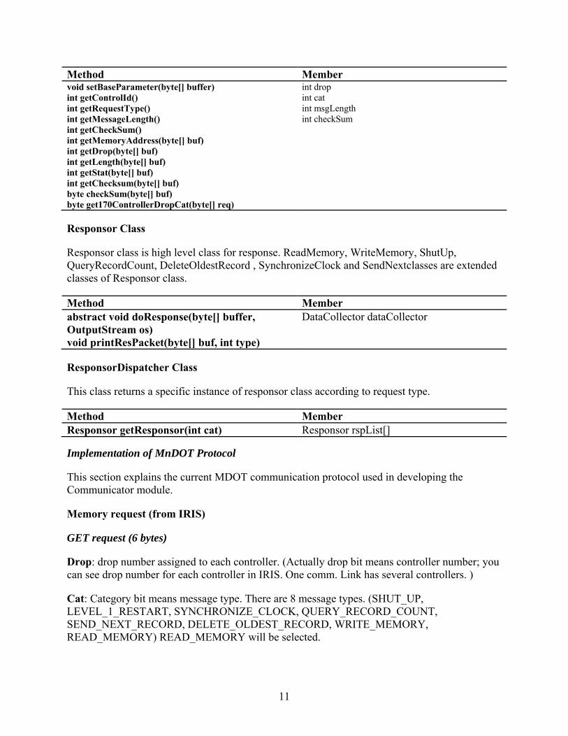
Responsor Class
Responsor class is high level class for response. ReadMemory, WriteMemory, ShutUp, QueryRecordCount, DeleteOldestRecord , SynchronizeClock and SendNextclasses are extended classes of Responsor class.
Method Member abstract void doResponse(byte[] buffer, OutputStream os) void printResPacket(byte[] buf, int type)
DataCollector dataCollector
ResponsorDispatcher Class
This class returns a specific instance of responsor class according to request type.
Method Member Responsor getResponsor(int cat) Responsor rspList[]
Implementation of MnDOT Protocol
This section explains the current MDOT communication protocol used in developing the Communicator module.
Memory request (from IRIS)
GET request (6 bytes)
Drop: drop number assigned to each controller. (Actually drop bit means controller number; you can see drop number for each controller in IRIS. One comm. Link has several controllers. )
Cat: Category bit means message type. There are 8 message types. (SHUT_UP, LEVEL_1_RESTART, SYNCHRONIZE_CLOCK, QUERY_RECORD_COUNT, SEND_NEXT_RECORD, DELETE_OLDEST_RECORD, WRITE_MEMORY, READ_MEMORY) READ_MEMORY will be selected.
12
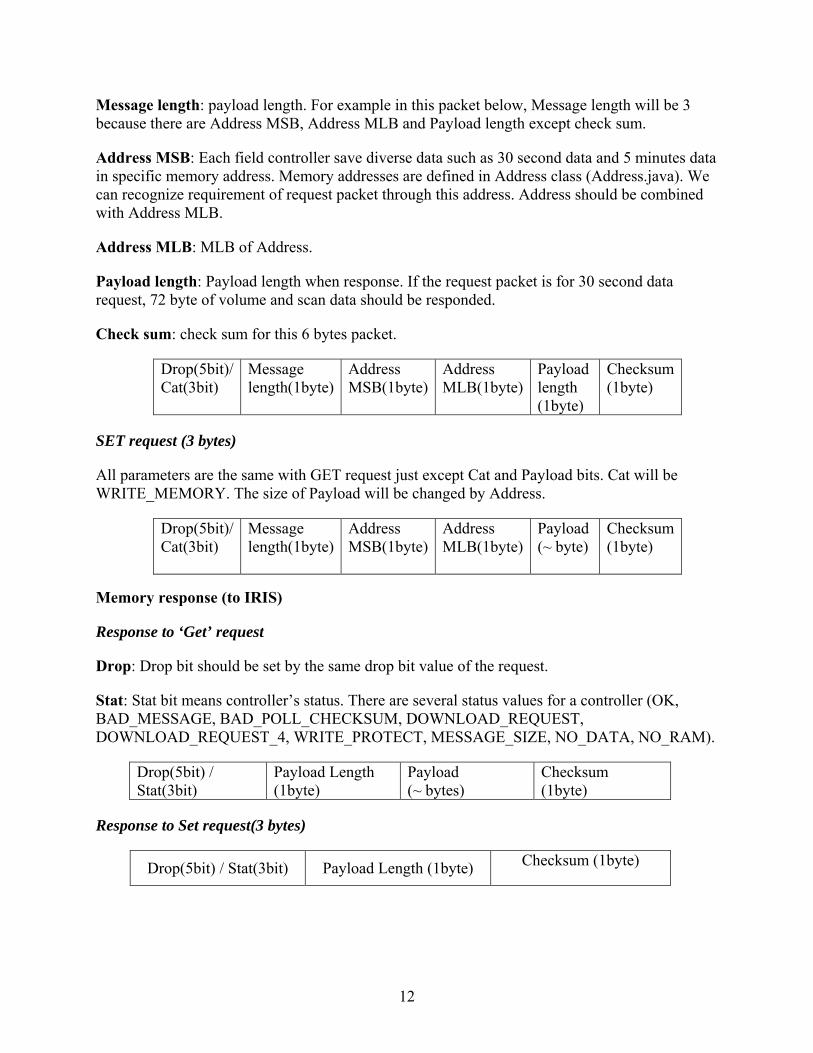
Message length: payload length. For example in this packet below, Message length will be 3 because there are Address MSB, Address MLB and Payload length except check sum.
Address MSB: Each field controller save diverse data such as 30 second data and 5 minutes data in specific memory address. Memory addresses are defined in Address class (Address.java). We can recognize requirement of request packet through this address. Address should be combined with Address MLB.
Address MLB: MLB of Address.
Payload length: Payload length when response. If the request packet is for 30 second data request, 72 byte of volume and scan data should be responded.
Check sum: check sum for this 6 bytes packet.
Drop(5bit)/ Cat(3bit)
Message length(1byte)
Address MSB(1byte)
Address MLB(1byte)
Payload length (1byte)
Checksum (1byte)
SET request (3 bytes)
All parameters are the same with GET request just except Cat and Payload bits. Cat will be WRITE_MEMORY. The size of Payload will be changed by Address.
Drop(5bit)/ Cat(3bit)
Message length(1byte)
Address MSB(1byte)
Address MLB(1byte)
Payload (~ byte)
Checksum (1byte)
Memory response (to IRIS)
Response to ‘Get’ request
Drop: Drop bit should be set by the same drop bit value of the request.
Stat: Stat bit means controller’s status. There are several status values for a controller (OK, BAD_MESSAGE, BAD_POLL_CHECKSUM, DOWNLOAD_REQUEST, DOWNLOAD_REQUEST_4, WRITE_PROTECT, MESSAGE_SIZE, NO_DATA, NO_RAM).
Drop(5bit) / Stat(3bit)
Payload Length (1byte)
Payload (~ bytes)
Checksum (1byte)
Response to Set request(3 bytes)
Drop(5bit) / Stat(3bit) Payload Length (1byte) Checksum (1byte)
13
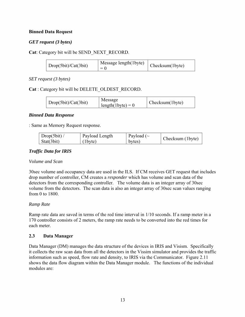
Binned Data Request
GET request (3 bytes)
Cat: Category bit will be SEND_NEXT_RECORD.
Drop(5bit)/Cat(3bit) Message length(1byte) = 0 Checksum(1byte)
SET request (3 bytes)
Cat : Category bit will be DELETE_OLDEST_RECORD.
Drop(5bit)/Cat(3bit) Message length(1byte) = 0 Checksum(1byte)
Binned Data Response
: Same as Memory Request response.
Drop(5bit) / Stat(3bit)
Payload Length (1byte)
Payload (~ bytes) Checksum (1byte)
Traffic Data for IRIS
Volume and Scan
30sec volume and occupancy data are used in the ILS. If CM receives GET request that includes drop number of controller, CM creates a responder which has volume and scan data of the detectors from the corresponding controller. The volume data is an integer array of 30sec volume from the detectors. The scan data is also an integer array of 30sec scan values ranging from 0 to 1800.
Ramp Rate
Ramp rate data are saved in terms of the red time interval in 1/10 seconds. If a ramp meter in a 170 controller consists of 2 meters, the ramp rate needs to be converted into the red times for each meter.
2.3 Data Manager
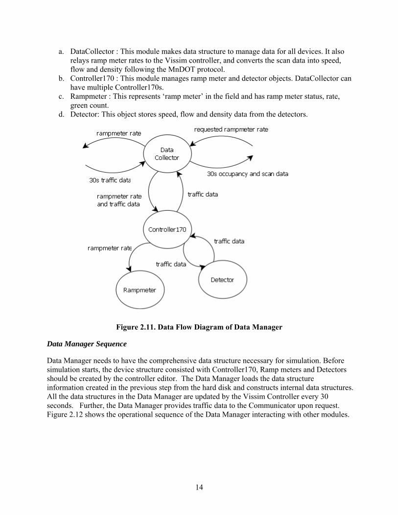
Data Manager (DM) manages the data structure of the devices in IRIS and Visism. Specifically it collects the raw scan data from all the detectors in the Vissim simulator and provides the traffic information such as speed, flow rate and density, to IRIS via the Communicator. Figure 2.11 shows the data flow diagram within the Data Manager module. The functions of the individual modules are:
14
a. DataCollector : This module makes data structure to manage data for all devices. It also relays ramp meter rates to the Vissim controller, and converts the scan data into speed, flow and density following the MnDOT protocol.
b. Controller170 : This module manages ramp meter and detector objects. DataCollector can have multiple Controller170s.
c. Rampmeter : This represents ‘ramp meter’ in the field and has ramp meter status, rate, green count.
d. Detector: This object stores speed, flow and density data from the detectors.
Figure 2.11. Data Flow Diagram of Data Manager
Data Manager Sequence
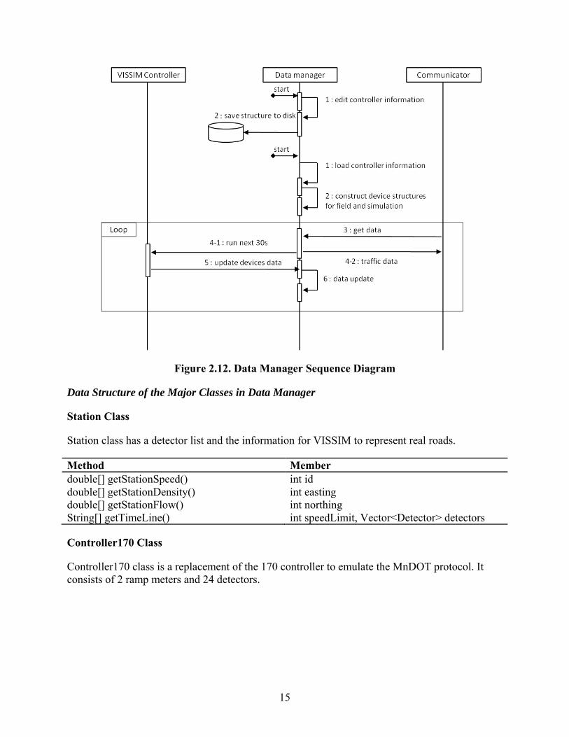
Data Manager needs to have the comprehensive data structure necessary for simulation. Before simulation starts, the device structure consisted with Controller170, Ramp meters and Detectors should be created by the controller editor. The Data Manager loads the data structure information created in the previous step from the hard disk and constructs internal data structures. All the data structures in the Data Manager are updated by the Vissim Controller every 30 seconds. Further, the Data Manager provides traffic data to the Communicator upon request. Figure 2.12 shows the operational sequence of the Data Manager interacting with other modules.
15
Figure 2.12. Data Manager Sequence Diagram
Data Structure of the Major Classes in Data Manager
Station Class
Station class has a detector list and the information for VISSIM to represent real roads.
Method Member double[] getStationSpeed() int id double[] getStationDensity() int easting double[] getStationFlow() int northing String[] getTimeLine() int speedLimit, Vector<Detector> detectors
Controller170 Class
Controller170 class is a replacement of the 170 controller to emulate the MnDOT protocol. It consists of 2 ramp meters and 24 detectors.
16
Method Member void setRampRate(int pin, byte rate) int drop double[] getVolume(int detectorId) Vector<RampMeter> rampMeters double[] getScan(int detectorId) Vector<Detector> detectors Device getDevice(int pin)
RampMeter Class
RampMeter class belongs to Controller170 class and is managed by Data Manager. It’s set by IRIS and synchronized with VISSIM.
Method Member void setRampRate(byte rate) int pin byte getRampRate() int id byte getRampStatus() byte rampStatus byte getCount() byte currentRate byte getPolicePanel() byte greenCount30Sec, byte policePanel
Detector Class
Detector class belongs to Controller170 and Station class. This class saves the volume and speed data provided by VISSIM and transforms data to other forms that are sent to IRIS by the MnDOT protocol.
Method Member TrafficData getTrafficData() int pin double[] getVolume() int id double[] getScan() String name, String Type, int fieldLength TrafficData trafficData
TrafficData Class
All traffic data is saved to this class and transformed to proper type by Detector class as requested.
Method Member void calculateTraffic() int fieldLength void setData(int row, int col, int value) int interval double[][] getData() float confidence double getData(int row, int col) double[][] data
2.4 VISSIM Controller
VISSIM Controller (VC), which has been developed with the COM interface, controls VISSIM simulator, manages device structures of VISSM and synchronizes device data in the Data Manager. The operational sequence of VC is as follows:
17
• Execute 1 step of VISSIM • Set control configuration to VISSIM • Get data from the detectors in VISSIM
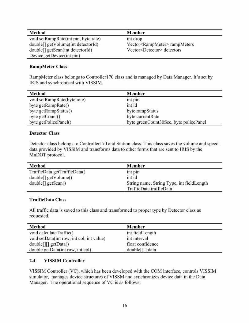
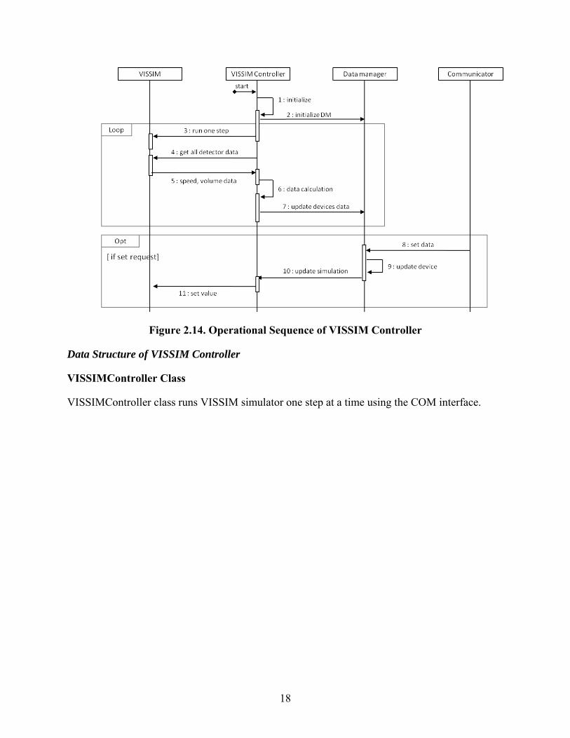
Figure 2.13 shows the data flow process within the Vissim controller whose internal modules include:
• Executor : This is the core module that controls the VISSIM simulation process and reads data from VISSIM.
• VDetector : This module represents the detectors in VISSIM. It stores volume and speed data on a temporary basis.
• VRunner : This is for executing some functions of external components and transferring data.
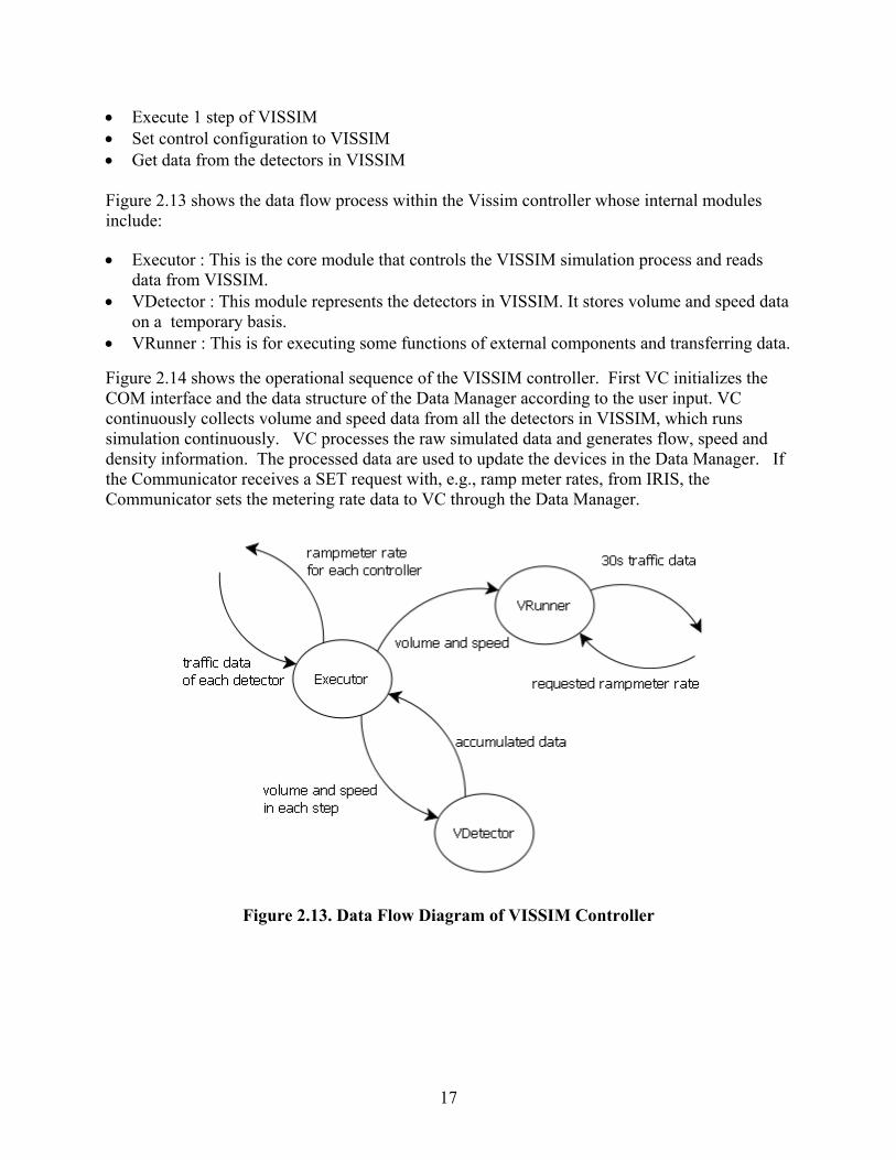
Figure 2.14 shows the operational sequence of the VISSIM controller. First VC initializes the COM interface and the data structure of the Data Manager according to the user input. VC continuously collects volume and speed data from all the detectors in VISSIM, which runs simulation continuously. VC processes the raw simulated data and generates flow, speed and density information. The processed data are used to update the devices in the Data Manager. If the Communicator receives a SET request with, e.g., ramp meter rates, from IRIS, the Communicator sets the metering rate data to VC through the Data Manager.
Figure 2.13. Data Flow Diagram of VISSIM Controller
18
Figure 2.14. Operational Sequence of VISSIM Controller
Data Structure of VISSIM Controller
VISSIMController Class
VISSIMController class runs VISSIM simulator one step at a time using the COM interface.
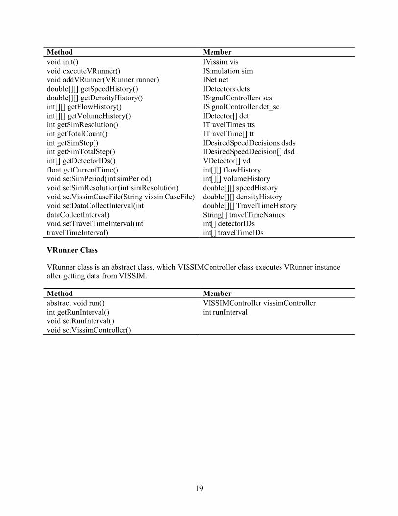
19
Method Member void init() void executeVRunner() void addVRunner(VRunner runner) double[][] getSpeedHistory() double[][] getDensityHistory() int[][] getFlowHistory() int[][] getVolumeHistory() int getSimResolution() int getTotalCount() int getSimStep() int getSimTotalStep() int[] getDetectorIDs() float getCurrentTime() void setSimPeriod(int simPeriod) void setSimResolution(int simResolution) void setVissimCaseFile(String vissimCaseFile) void setDataCollectInterval(int dataCollectInterval) void setTravelTimeInterval(int travelTimeInterval)
IVissim vis ISimulation sim INet net IDetectors dets ISignalControllers scs ISignalController det_sc IDetector[] det ITravelTimes tts ITravelTime[] tt IDesiredSpeedDecisions dsds IDesiredSpeedDecision[] dsd VDetector[] vd int[][] flowHistory int[][] volumeHistory double[][] speedHistory double[][] densityHistory double[][] TravelTimeHistory String[] travelTimeNames int[] detectorIDs int[] travelTimeIDs
VRunner Class
VRunner class is an abstract class, which VISSIMController class executes VRunner instance after getting data from VISSIM.
Method Member abstract void run() int getRunInterval() void setRunInterval() void setVissimController()
VISSIMController vissimController int runInterval
20
3 DEVELOPMENT OF AN OFF-LINE ESTIMATION PROCESS FOR FREEWAY TRAFFIC CONDITIONS
3.1 Structure of Traffic Information and Condition Analysis System (TICAS)
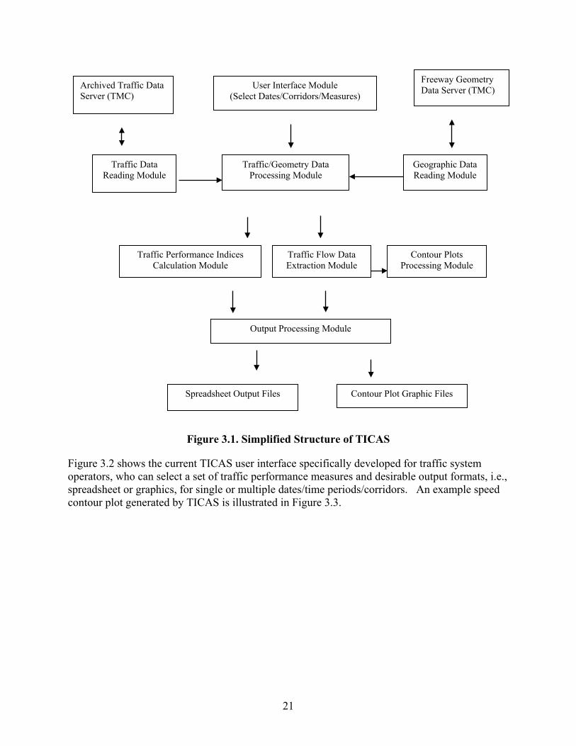
In this task, a comprehensive freeway Traffic Information and Condition Analysis System (TICAS) is developed to support the needs of the traffic operators in terms of quantifying and assessing the traffic performance of the freeway corridors in Minnesota with the historical detector data continuously being archived at the Traffic Management Center. Figure 3.1 shows the simplified structure and data flow process of TICAS developed in this study. As shown in this figure, the main data source for TICAS consists of the infrastructure-based traffic flow detectors, e.g., loops or radars, which provide traffic flow rate, speed and density data at fixed locations every 30 seconds. The archived traffic data, stored at the data server at the Traffic Management Center, is accessed by TICAS through internet each time user defines the data needs. The traffic data are combined and linked to the specific geometry data of each freeway corridor to develop corridor-based traffic information, such as travel times and vehicle miles traveled, etc. These measures are of critical importance in assessing the congestion levels and evaluating the effectiveness of traffic control strategies. The main format of the output files from the current version of TICAS is the spreadsheet file, which can be directly opened by Excel. Further, the contour plots for the basic flow parameters, such as speed, density and flow rates, can be directly created by TICAS, which also provides users the capability to adjust contour plot intervals.
21
User Interface Module (Select Dates/Corridors/Measures)
Traffic/Geometry Data Processing Module
Geographic Data Reading Module
Traffic Data Reading Module
Traffic Performance Indices Calculation Module
Traffic Flow Data Extraction Module
Contour Plots Processing Module
Archived Traffic Data Server (TMC)
Freeway Geometry Data Server (TMC)
Figure 3.1. Simplified Structure of TICAS
Spreadsheet Output Files
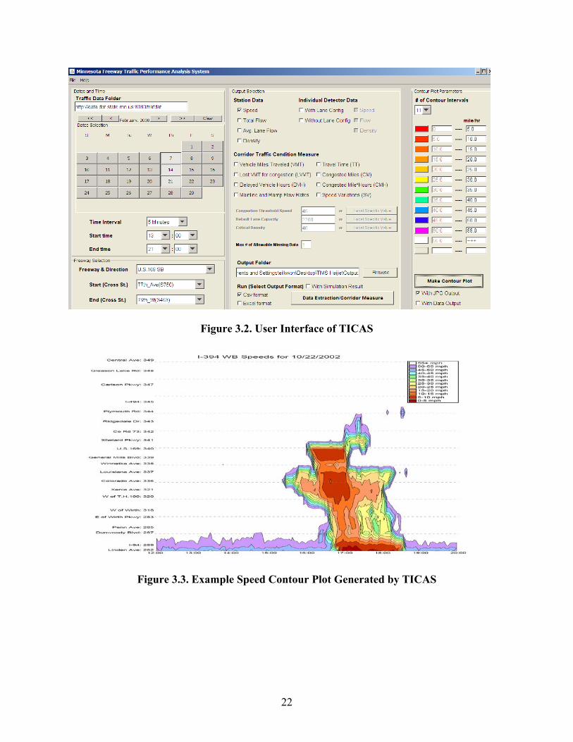
Figure 3.2 shows the current TICAS user interface specifically developed for traffic system operators, who can select a set of traffic performance measures and desirable output formats, i.e., spreadsheet or graphics, for single or multiple dates/time periods/corridors. An example speed contour plot generated by TICAS is illustrated in Figure 3.3.
Output Processing Module
Contour Plot Graphic Files
22
Figure 3.2. User Interface of TICAS
Figure 3.3. Example Speed Contour Plot Generated by TICAS
23
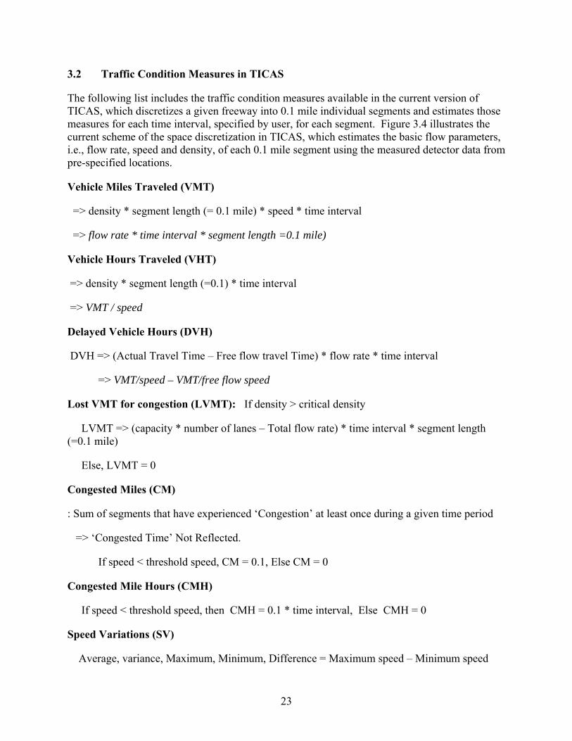
3.2 Traffic Condition Measures in TICAS
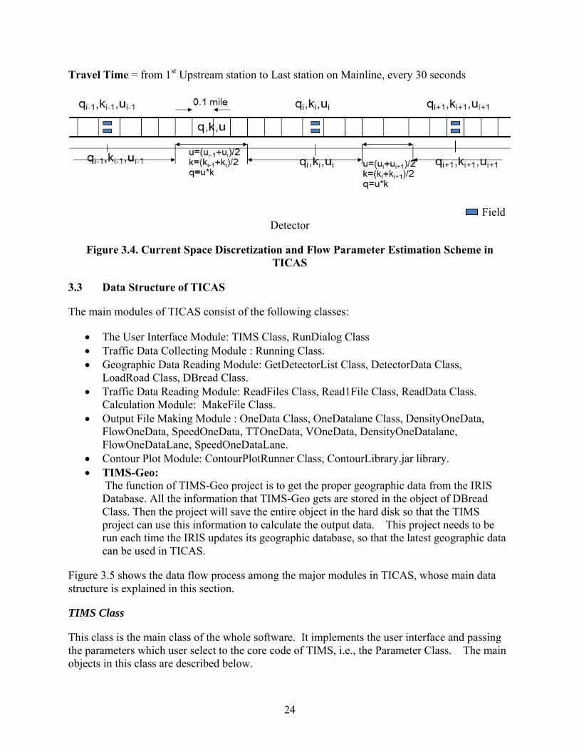
The following list includes the traffic condition measures available in the current version of TICAS, which discretizes a given freeway into 0.1 mile individual segments and estimates those measures for each time interval, specified by user, for each segment. Figure 3.4 illustrates the current scheme of the space discretization in TICAS, which estimates the basic flow parameters, i.e., flow rate, speed and density, of each 0.1 mile segment using the measured detector data from pre-specified locations.
Vehicle Miles Traveled (VMT)
=> density * segment length (= 0.1 mile) * speed * time interval
=> flow rate * time interval * segment length =0.1 mile)
Vehicle Hours Traveled (VHT)
=> density * segment length (=0.1) * time interval
=> VMT / speed
Delayed Vehicle Hours (DVH)
DVH => (Actual Travel Time – Free flow travel Time) * flow rate * time interval
=> VMT/speed – VMT/free flow speed
Lost VMT for congestion (LVMT): If density > critical density
LVMT => (capacity * number of lanes – Total flow rate) * time interval * segment length (=0.1 mile)
Else, LVMT = 0
Congested Miles (CM)
: Sum of segments that have experienced ‘Congestion’ at least once during a given time period
=> ‘Congested Time’ Not Reflected.
If speed < threshold speed, CM = 0.1, Else CM = 0
Congested Mile Hours (CMH)
If speed < threshold speed, then CMH = 0.1 * time interval, Else CMH = 0
Speed Variations (SV)
Average, variance, Maximum, Minimum, Difference = Maximum speed – Minimum speed
24
Travel Time = from 1st Upstream station to Last station on Mainline, every 30 seconds
Field Detector
Figure 3.4. Current Space Discretization and Flow Parameter Estimation Scheme in TICAS
3.3 Data Structure of TICAS
The main modules of TICAS consist of the following classes:
• The User Interface Module: TIMS Class, RunDialog Class • Traffic Data Collecting Module : Running Class. • Geographic Data Reading Module: GetDetectorList Class, DetectorData Class,
LoadRoad Class, DBread Class. • Traffic Data Reading Module: ReadFiles Class, Read1File Class, ReadData Class.
Calculation Module: MakeFile Class. • Output File Making Module : OneData Class, OneDatalane Class, DensityOneData,
FlowOneData, SpeedOneData, TTOneData, VOneData, DensityOneDatalane, FlowOneDataLane, SpeedOneDataLane.
• Contour Plot Module: ContourPlotRunner Class, ContourLibrary.jar library. • TIMS-Geo:
The function of TIMS-Geo project is to get the proper geographic data from the IRIS Database. All the information that TIMS-Geo gets are stored in the object of DBread Class. Then the project will save the entire object in the hard disk so that the TIMS project can use this information to calculate the output data. This project needs to be run each time the IRIS updates its geographic database, so that the latest geographic data can be used in TICAS.
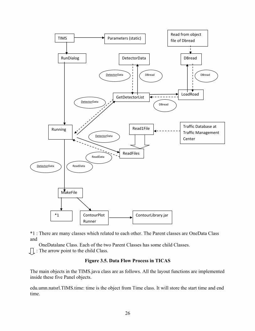
Figure 3.5 shows the data flow process among the major modules in TICAS, whose main data structure is explained in this section.
TIMS Class
This class is the main class of the whole software. It implements the user interface and passing the parameters which user select to the core code of TIMS, i.e., the Parameter Class. The main objects in this class are described below.

25
NameSpace
edu.umn.natsrl.TIMS.panel : The main panel that contain all the layout of the program.
edu.umn.natsrl.TIMS.TimePanel: left upper panel in the program.
edu.umn.natsrl.TIMS.OutputPanel: Middle panel in the program.
edu.umn.natsrl.TIMS.AreaPanel: left lower panel in the program.
edu.umn.natsrl.TIMS.PlotPanel: right panel in the program.
edu.umn.natsrl.TIMS.pam: This is the object from class paracheck(). The function is to pass the available date in the network to the DateSelection class so that the DateSelection class can use this information to check which date is available in the Calendar function.
edu.umn.natsrl.TIMS.cv: float[] cv object store the information of the Contour intervals. The cv is the value of each Contour intervals.
edu.umn.natsrl.TIMS.ncv: int ncv object stores the number of Contour intervals.
edu.umn.natsrl.TIMS.color: Color[] color object stores the color of each Contour intervals.
edu.umn.natsrl.TIMS.calendar: calendar is the object of DateSelection Class.
26
*1 : There are many classes which related to each other. The Parent classes are OneData Class and OneDatalane Class. Each of the two Parent Classes has some child Classes. : The arrow point to the child Class.
Figure 3.5. Data Flow Process in TICAS
GetDetectorList
TIMS
RunDialog
Running
DetectorData
LoadRoad
DBread
Read from object file of Dbread
ReadFiles
MakeFile
Traffic Database at Traffic Management Center
Read1File
*1 ContourPlotRunner
Parameters (static)
ContourLibrary.jar
DetectorData
DBread
DBread
DBread
DetectorData
DetectorData
ReadData
ReadData
DetectorData
The main objects in the TIMS.java class are as follows. All the layout functions are implemented inside these five Panel objects.
edu.umn.natsrl.TIMS.time: time is the object from Time class. It will store the start time and end time.
27
edu.umn.natsrl.TIMS.datelist: datelist is the object from DateList class. It will store the dates that the user want to make analysis from.
edu.umn.natsrl.TIMS.flag: flag stores the information of what user select in the layout.
edu.umn.natsrl.TIMS.RoadFile: RoadFile is the File object. It stores the Road Files that the user wants to analyze.
edu.umn.natsrl.TIMS.RoadName: The string name of the Road File.
edu.umn.natsrl.TIMS.StartSt: The Starting street that the user selects.
edu.umn.natsrl.TIMS.EndSt: The End street that the user selects.
Parameters Class
This class stores the important values that will be used throughout the whole TIMS project. Because of this, the information inside the Parameters Class is static. The data stored in this class can be directly accessed by other classes.
RunDialog Class
The main function of this Class is to show the user a dialog window. Then the RunDialog will call the Running Class.
Running Class
This Class is one of the core functions in the TIMS Project. The main function of this Class is to get the needed information from the Traffic Data and Geographic Data. And then send the data to the MakeFile Class whose job is to use the Traffic Data and Geographic Data to do the analysis.
NameSpace
edu.umn.natsrl.Running.AllDetect: Vector<DetectorData> AllDetect is the object array of DetectorData Class. This object stores the information of the Geographic Data of the Detectors which will be used to do the analysis.
edu.umn.natsrl.Running.AllDATA: Vector<ReadData> AllDATA is the object array of ReadData Class. This object stores the information of the Traffic Data
GetDetectorList Class
This Class is the main class of the Geographic Data Reading Module. This Class will get the whole Data of a road from the Geo Database which is created by the TIMS-Geo Project. Then select the Data that will be used by the calculation module of TIMS. After finishing these tasks, send the object array which contains all the Geo information to the Running Class.
28
NameSpace :edu.umn.natsrl.GetDetectorList.AllDetect: Vector<DetectorData> AllDetect is the object array of DetectorData Class. This object stores the information of the Geographic Data of the Detectors which are in the range from the Start Street to End Street.
edu.umn.natsrl.GetDetectorList.alldetector: Vector<DBread> alldetector is the object array of DBread Class. This object stores the Geographic Data of the whole specified road.
LoadRoad Class
The function of the LoadRoad Class is to read all detectors data of a selected road from the disk. The detectors data is stored in the disk as the object file. The object that stored is the Vector<DBread> Class object.
DBread Class
The object array of this class stores the information of the geographic data of detectors. One important thing in the TIMS software is to make sure that the edu.umn.natsrl.geodb.DBread of the TIMS project is exactly the same with the edu.umn.natsrl.geodb.DBread of the TIMS-Geo project. The reachild is that the LoadRoad Class of TIMS project will try to read the saved object of DBread class. And the saved object is from the DBread Class in TIMS-Geo project. Thus, if the two DBread class is not exactly same, the LoadRoad Class cannot read the data properly.
DetectorData Class
The object of the DetectorData will store the geographic data of detectors from selected road and from selected starting point to end point.
ReadFiles Class (child class of Read1File Class)
The function of this class is to read the traffic data from either the Internet or Local disk. The parent class of ReadFiles is Read1File Class.
NameSpace
edu.umn.natsrl.ReadFiles.fulldata: Vector<ReadData> fulldata is the object array of ReadData Class. The function of this object is to store the traffic data information.
Read1File Class
The function of this class is to read the .v30 and .c30 files (which are the volume and occupancy files).
NameSpace
edu.umn.natsrl.Read1File.getNet (int DID): The function is to get the traffic data of the detector which Detector ID is “DID”.

29
edu.umn.natsrl.Read1File.read_data: ReadData read_data object stores the traffic data of the detector which Detector ID is “DID”.
Constants Class
This Class stores the constant value that will be used in the TIMS. The information inside include the ID of each output and constant value of road parameters.
ReadData Class
The function of the ReadData Class is to store the traffic data extracted from either the internet or local disk. The other module in the TIMS will use the object of the ReadData Class to store the information of traffic data.
NameSpace
edu.umn.natsrl.ReadData.Calculate(): This function is to calculate the speed from the density and flow. In the Read1File Class, the flow and density traffic data will be read from the database directly. Then, the Read1File Class will call this function to get the speed value.
DateSelection Class
The function of the DateSelection Class is to build a Calendar interface for the user to choose the date. The DateSelection Class will call to the DateChecker Class to see if the traffic data is available for a specific day or not.
MakeFile Class
This Class is the main Class for the Calculation Module. It gets the traffic data and the geographic data from the Running Class. First, the MakeFile Class will use the traffic data and geographic data to calculate 7 basic output data. The output data will be stored in the object of OneData and OneDatalane’s child Class. Then, depending on what the user choose in the interface, the MakeFile will calculate the required output data based on the 7 basic output data.
The Class that is used for storing the output data include: OneData Class, OneDatalane Class, DensityOneData, FlowOneData, SpeedOneData, TTOneData, VOneData, DensityOneDatalane, FlowOneDataLane, SpeedOneDataLane. All the objects of these Classes will be used to store the calculated data. The calculation process to produce one basic output data is as follows:
Density = this.Initialize(AllData, Constants.Density,false);
This command is used to get the Density basic output data. The process to calculate and store the Density data is as follow:
• The Initialize(Vector<ReadData> Data, int flag, boolean isAFlow) function will construct the object array of OneData Class in order to store output data. Each object of the array will store one day data. Then it will construct other parameters which will be used in calculation.

30
• It will use the geographic data (stored in the object array of DetectorData) passed by Running Class to calculate the number of Rows and Columns.
• It will get the traffic data from the detector data (stored in the object array of ReadData). Then use the geographic data to know which detectors are in the same station. After that, the function will calculate the average density and store all the data to the object array of DensityOneData which is the child Class of OneData.
After all the output data that the user want calculated and stored, the MakeFile Class will call to the function inside the OneData related Class to make the output files.
OneData Class and OneDatalane Class and relatives
The function of OneData Class is to store the output data and then make the .csv or .xls files based on the output data. First, the MakeFile Class will call OneData class to store the calculated data. Then, MakeFile will call the OneData to make proper output files.
ContourPlotRunner Class
The function of ContourPlotRunner Class is to call the ContourPlot Library and pass the needed data and parameters to the ContourPlot drawing function inside the ContourPlot Library. There are many crucial parameters to the Plot.
edu.umn.natsrl.ContourPlotRunner.power: The int power indicates how smooth the ContourPlot will be. The smaller the value is, the more smooth the plot will have. However, the bigger the value is, the more accurate the plot will be.
Other parameters inside this Class are so important to the ContourPlot drawing function. So I recommend that do not try to change other parameters such as du.umn.natsrl.ContourPlotRunner.numX.
ContourLibrary.jar
This library is developed from JfreeChart Library, whose contour drawing functions are modified in this study. The most important classes of the Contour Module are: org.jfree.chart.contour.ContourPlotgood.java , org.jfree.chart.plot.ContourPlot.java , org.jfree.chart.axis.NumberAxis.java and org.jfree.chart.axis.ValueAxis.
The function of the ContourPlot.java is to connect all other functions.
The function of the ContourPlotgood is to draw the contour plot.
31
4 DEVELOPMENT OF AN ON-LINE ESTIMATION PROCESS FOR FREEWAY TRAFFIC CONDITIONS
4.1 Data Structure and Operational Sequence of On-Line Process
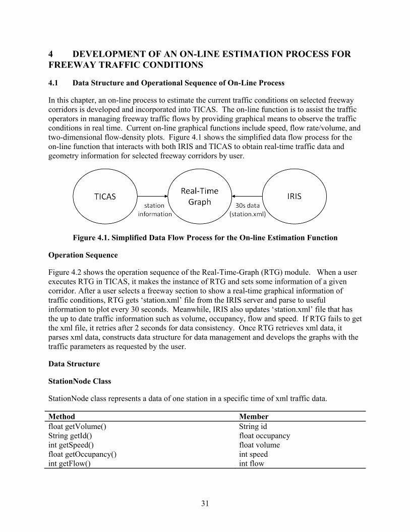
In this chapter, an on-line process to estimate the current traffic conditions on selected freeway corridors is developed and incorporated into TICAS. The on-line function is to assist the traffic operators in managing freeway traffic flows by providing graphical means to observe the traffic conditions in real time. Current on-line graphical functions include speed, flow rate/volume, and two-dimensional flow-density plots. Figure 4.1 shows the simplified data flow process for the on-line function that interacts with both IRIS and TICAS to obtain real-time traffic data and geometry information for selected freeway corridors by user.
Figure 4.1. Simplified Data Flow Process for the On-line Estimation Function
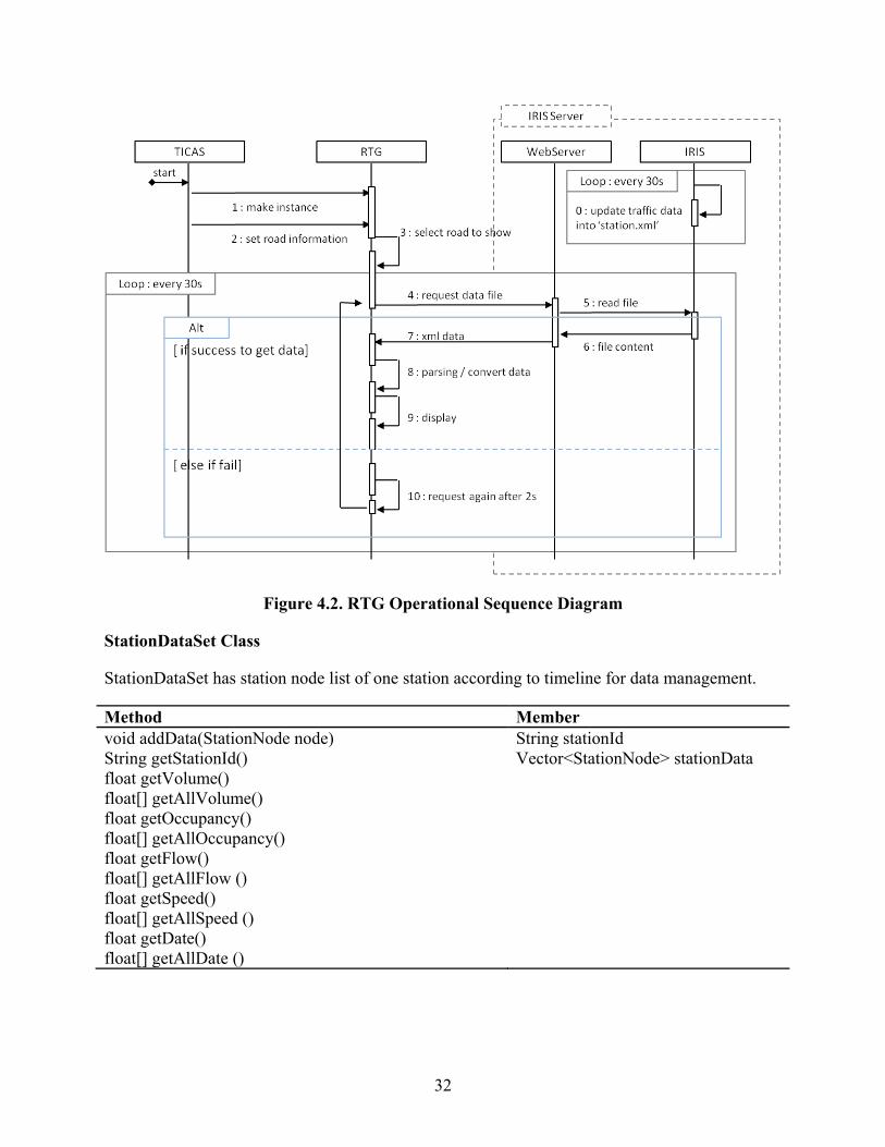
Operation Sequence
Figure 4.2 shows the operation sequence of the Real-Time-Graph (RTG) module. When a user executes RTG in TICAS, it makes the instance of RTG and sets some information of a given corridor. After a user selects a freeway section to show a real-time graphical information of traffic conditions, RTG gets ‘station.xml’ file from the IRIS server and parse to useful information to plot every 30 seconds. Meanwhile, IRIS also updates ‘station.xml’ file that has the up to date traffic information such as volume, occupancy, flow and speed. If RTG fails to get the xml file, it retries after 2 seconds for data consistency. Once RTG retrieves xml data, it parses xml data, constructs data structure for data management and develops the graphs with the traffic parameters as requested by the user.
Data Structure
StationNode Class
StationNode class represents a data of one station in a specific time of xml traffic data.
Method Member float getVolume() String id String getId() float occupancy int getSpeed() float volume float getOccupancy() int speed int getFlow() int flow
32
Figure 4.2. RTG Operational Sequence Diagram
StationDataSet Class
StationDataSet has station node list of one station according to timeline for data management.
Method Member void addData(StationNode node) String stationId String getStationId() Vector<StationNode> stationData float getVolume() float[] getAllVolume() float getOccupancy() float[] getAllOccupancy() float getFlow() float[] getAllFlow () float getSpeed() float[] getAllSpeed () float getDate() float[] getAllDate ()
33
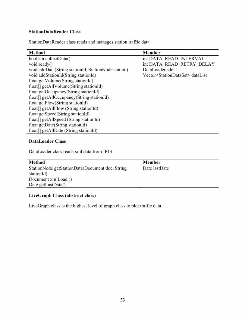
StationDataReader Class
StationDataReader class reads and manages station traffic data.
Method Member boolean collectData() int DATA_READ_INTERVAL void ready() int DATA_READ_RETRY_DELAY void addData(String stationId, StationNode station) DataLoader sdr void addStationId(String stationId) Vector<StationDataSet> dataList float getVolume(String stationId) float[] getAllVolume(String stationId) float getOccupancy(String stationId) float[] getAllOccupancy(String stationId) float getFlow(String stationId) float[] getAllFlow (String stationId) float getSpeed(String stationId) float[] getAllSpeed (String stationId) float getDate(String stationId) float[] getAllDate (String stationId)
DataLoader Class
DataLoader class reads xml data from IRIS.
Method Member StationNode getStationData(Document doc, String stationId)
Date lastDate
Document xmlLoad () Date getLastDate()
LiveGraph Class (abstract class)
LiveGraph class is the highest level of graph class to plot traffic data.
34
Method Member JGraphPanel getGraphPanel() Graph graph void addStation(StationNode station) Hashtable<String, XYDataSeries>
dataList void addData(StationNode station) int yMax void createChart(StationNode station) int yMin void addLegend(LinePlot plot, StationNode station) String title void addHint(LinePlot plot) LinePlot createPlot(StationNode station) abstract void addValue(XYDataSeries ds, StationNode station) abstract int getXSeriesType() abstract int getYSeriesType() abstract String getTitle() abstract String getXLegend() abstract String getYLegend() abstract String getHintTemplate()
LiveTimelineGraph Class (abstract class)
LiveTimelineGraph is abstract class implementing LiveGraph to plot time-based data.
Method Member void addValue(XYDataSeries ds, StationNode station) String dataType String getTitle() String getXLegend() String getYLegend() String getHintTemplate() int getXSeriesType() int getYSeriesType() abstract float getData(StationNode station)
LiveXYGraph Class (abstract class)
LiveXYGraph is abstract class implementing LiveGraph to plot data.
Method Member void addValue(XYDataSeries ds, StationNode station) String dataType String getTitle() String getXLegend() String getYLegend() String getHintTemplate() int getXSeriesType() int getYSeriesType() abstract float getXData(StationNode station) abstract float getYData(StationNode station)
35
SpeedGraph, FlowGraph, Density, Volume Class
These are classes extending LiveTimelineGraph class. And each class implements ‘getData’ method of LiveTimelineGraph class to return corresponding data.
Method Member float getData(StationNode station)
QKGraph Class
QKGraph class is a class extending LiveXYGraph class. And each class implements ‘getXData’ and ‘getYData’ method of LiveXYGraph class to return density and flow data.
Method Member float getXData(StationNode station) float getYData(StationNode station)
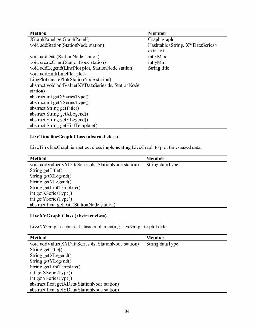
4.2 Example On-Line Graphs for Selected Traffic Parameters
The following example graphs show the screen captures of the graphical representations of the traffic variations up to the current time at the selected detector stations.
Figure 4.3. Real-time Graph for Speed Variations through Time
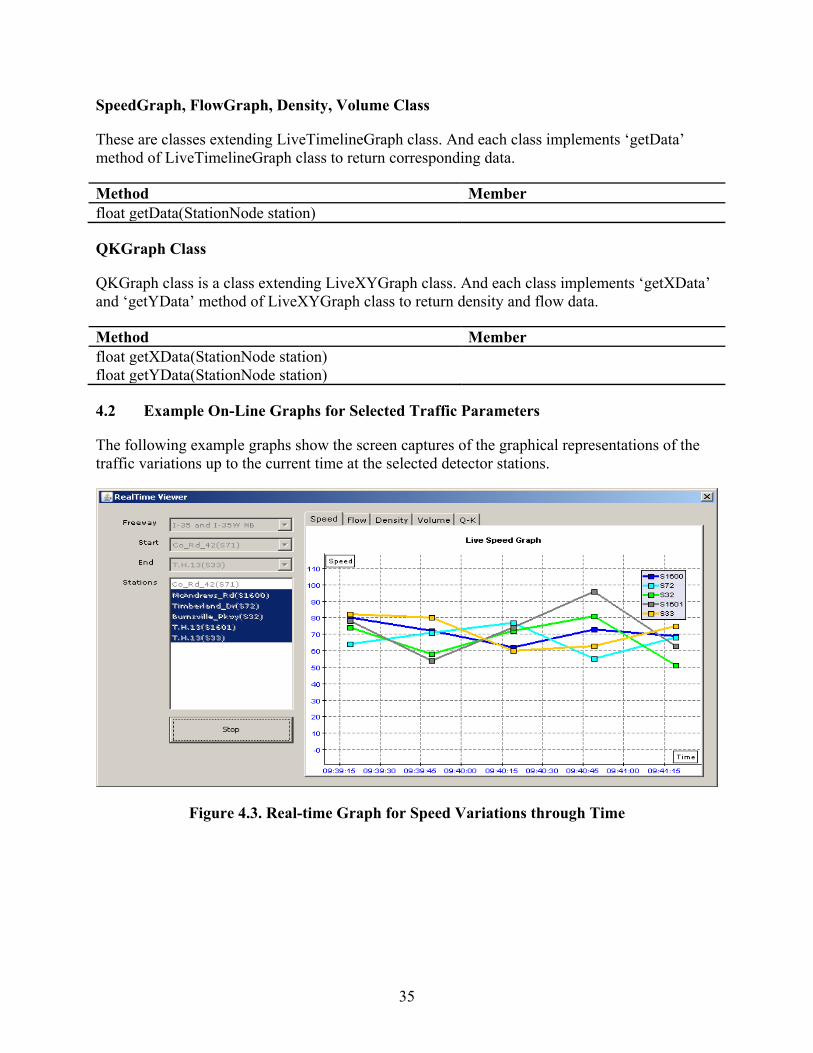
36
Figure 4.4. Real-time Graph for Flow Rate Variations through Time
Figure 4.5. Real-time Graph for Density Variations through Time
37
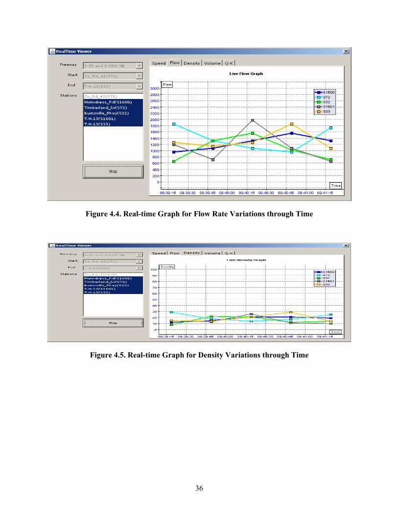
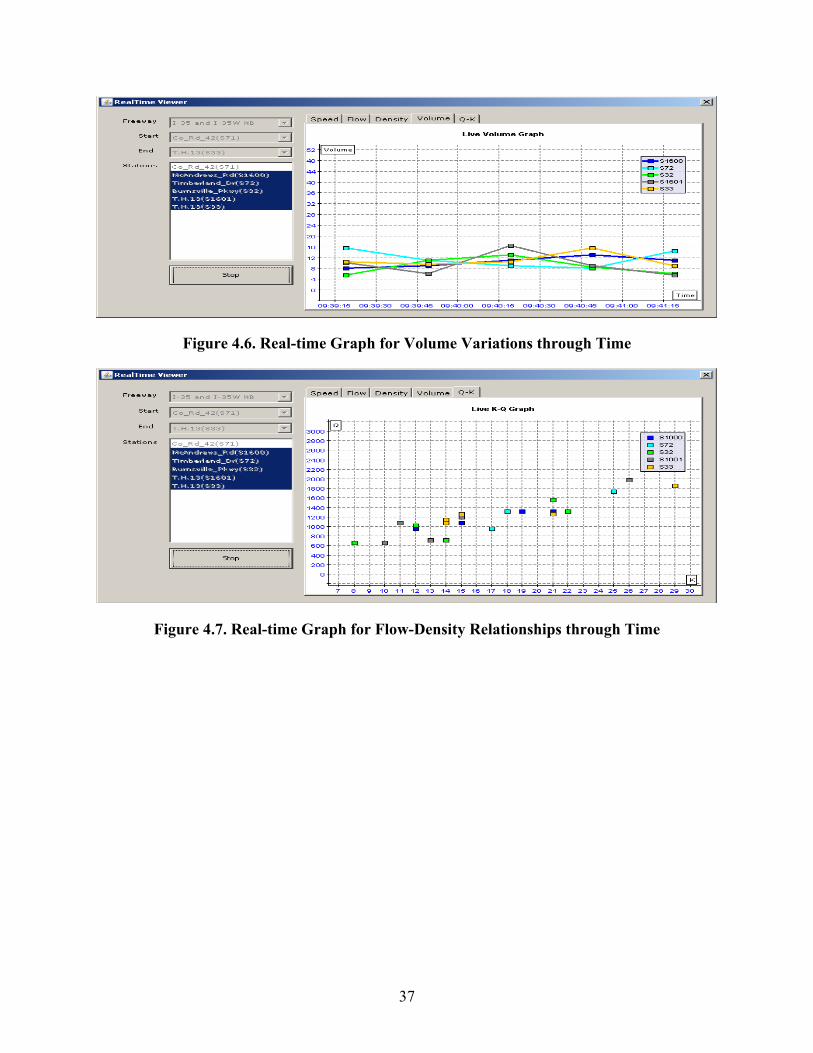
Figure 4.6. Real-time Graph for Volume Variations through Time
Figure 4.7. Real-time Graph for Flow-Density Relationships through Time
38
5 MICROSCOPIC MODELING A FREEWAY CORRIDOR FOR EXAMPLE APPLICATION OF ILSS WITH FREEWAY OPERATIONAL STRATEGIES
5.1 Sample Freeway Corridor
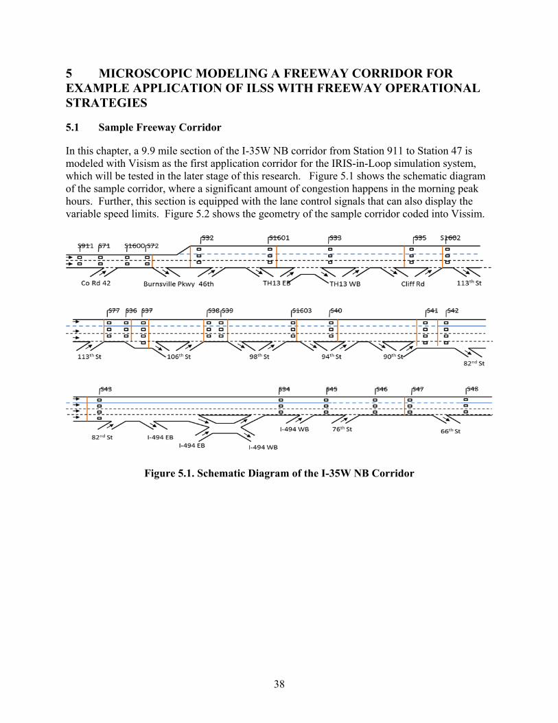
In this chapter, a 9.9 mile section of the I-35W NB corridor from Station 911 to Station 47 is modeled with Visism as the first application corridor for the IRIS-in-Loop simulation system, which will be tested in the later stage of this research. Figure 5.1 shows the schematic diagram of the sample corridor, where a significant amount of congestion happens in the morning peak hours. Further, this section is equipped with the lane control signals that can also display the variable speed limits. Figure 5.2 shows the geometry of the sample corridor coded into Vissim.
Figure 5.1. Schematic Diagram of the I-35W NB Corridor
39
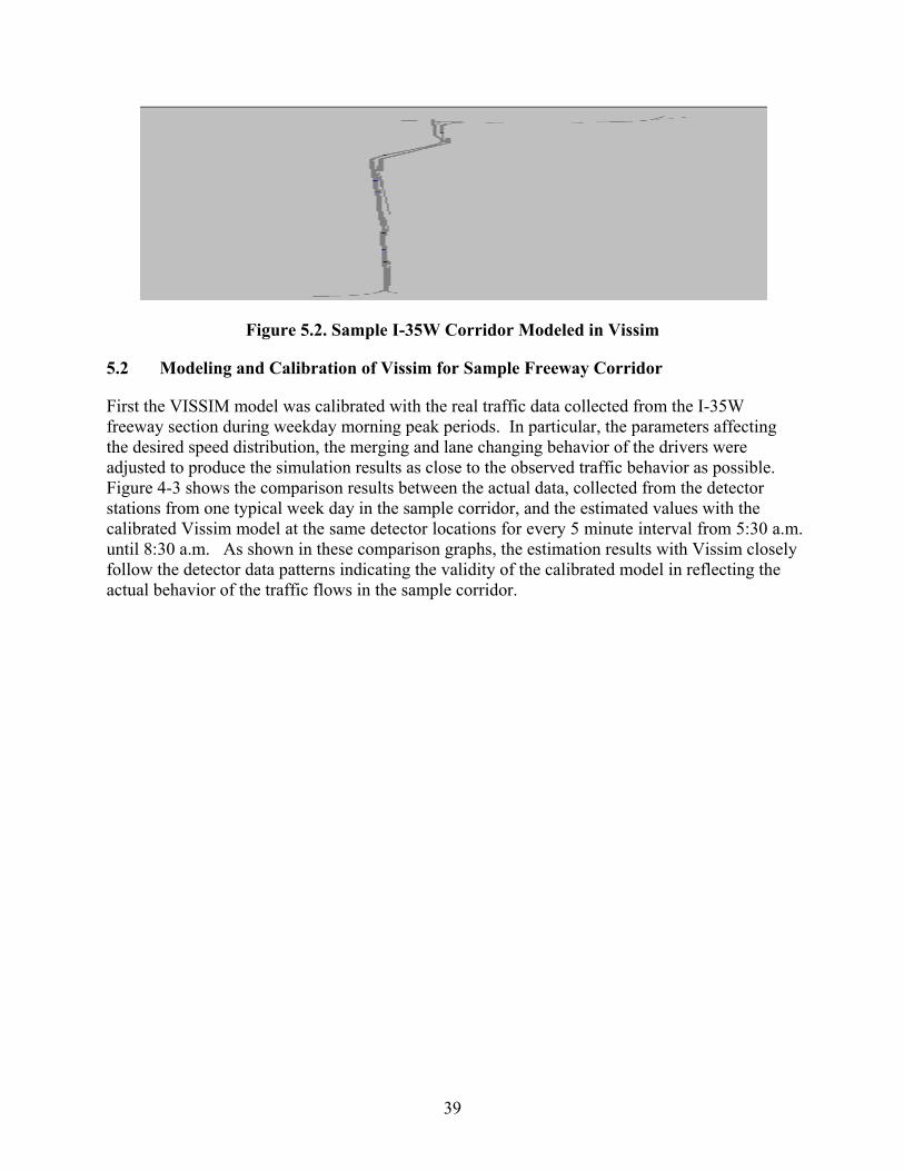
Figure 5.2. Sample I-35W Corridor Modeled in Vissim
5.2 Modeling and Calibration of Vissim for Sample Freeway Corridor
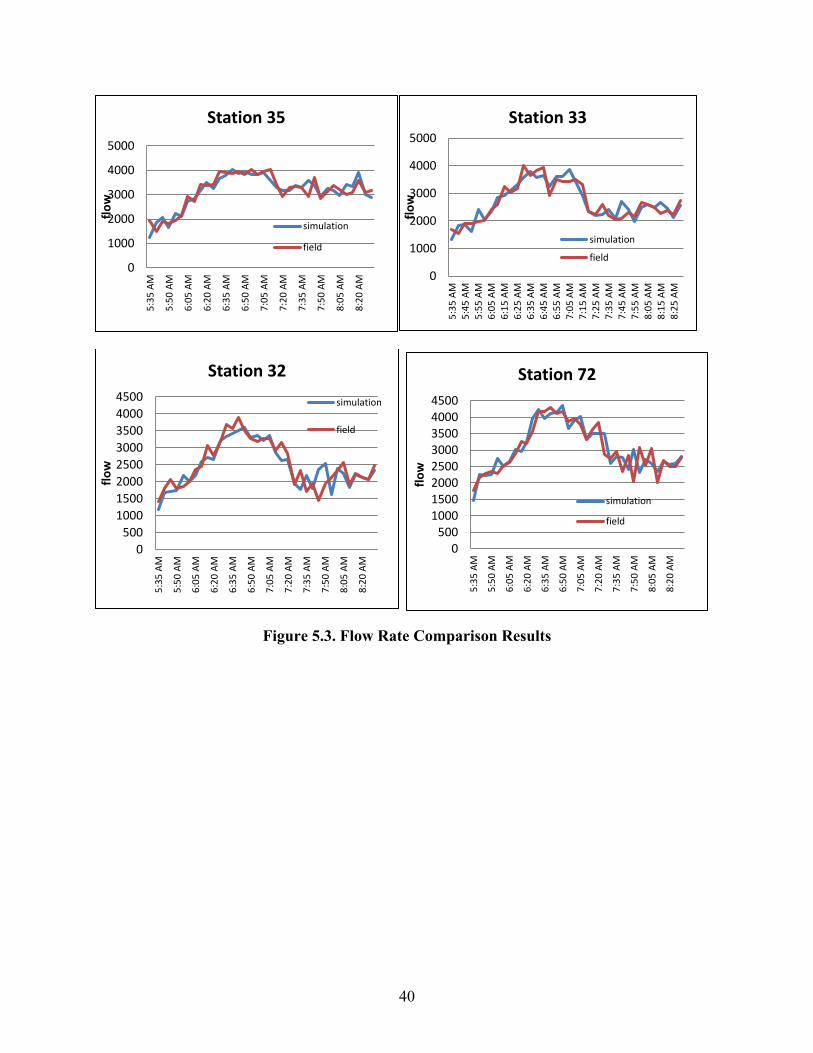
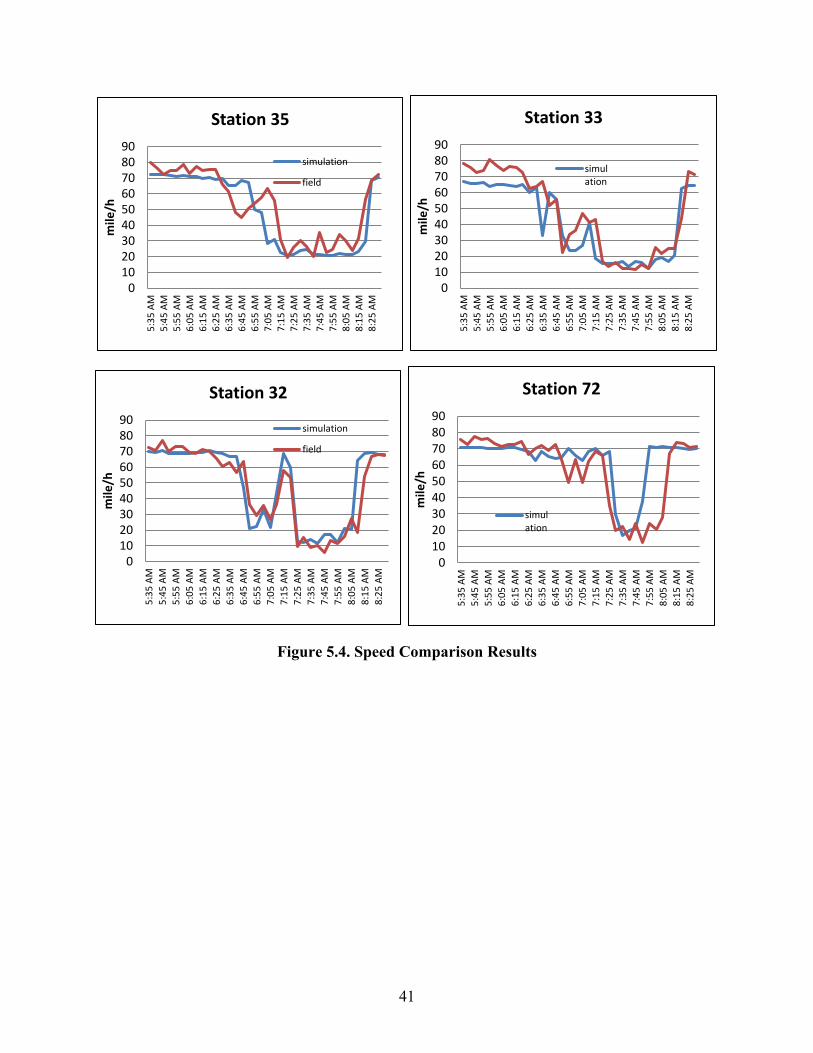
First the VISSIM model was calibrated with the real traffic data collected from the I-35W freeway section during weekday morning peak periods. In particular, the parameters affecting the desired speed distribution, the merging and lane changing behavior of the drivers were adjusted to produce the simulation results as close to the observed traffic behavior as possible. Figure 4-3 shows the comparison results between the actual data, collected from the detector stations from one typical week day in the sample corridor, and the estimated values with the calibrated Vissim model at the same detector locations for every 5 minute interval from 5:30 a.m. until 8:30 a.m. As shown in these comparison graphs, the estimation results with Vissim closely follow the detector data patterns indicating the validity of the calibrated model in reflecting the actual behavior of the traffic flows in the sample corridor.
40
0
1000
2000
3000
4000
5000
5:35
AM
5:45
AM
5:55
AM
6:05
AM
6:15
AM
6:25
AM
6:35
AM
6:45
AM
6:55
AM
7:05
AM
7:15
AM
7:25
AM
7:35
AM
7:45
AM
7:55
AM
8:05
AM
8:15
AM
8:25
AM
flow
Station 33
simulation
field
0500
10001500200025003000350040004500
5:35
AM
5:50
AM
6:05
AM
6:20
AM
6:35
AM
6:50
AM
7:05
AM
7:20
AM
7:35
AM
7:50
AM
8:05
AM
8:20
AM
flow
Station 72
simulation
field
Figure 5.3. Flow Rate Comparison Results
0
1000
2000
3000
4000
50005:
35 A
M
5:50
AM
6:05
AM
6:20
AM
6:35
AM
6:50
AM
7:05
AM
7:20
AM
7:35
AM
7:50
AM
8:05
AM
8:20
AM
flow
Station 35
simulation
field
0500
10001500200025003000350040004500
5:35
AM
5:50
AM
6:05
AM
6:20
AM
6:35
AM
6:50
AM
7:05
AM
7:20
AM
7:35
AM
7:50
AM
8:05
AM
8:20
AM
flow
Station 32 simulation
field
41
0102030405060708090
5:35
AM
5:45
AM
5:55
AM
6:05
AM
6:15
AM
6:25
AM
6:35
AM
6:45
AM
6:55
AM
7:05
AM
7:15
AM
7:25
AM
7:35
AM
7:45
AM
7:55
AM
8:05
AM
8:15
AM
8:25
AM
mile
/h
Station 33
simulation
0102030405060708090
5:35
AM
5:45
AM
5:55
AM
6:05
AM
6:15
AM
6:25
AM
6:35
AM
6:45
AM
6:55
AM
7:05
AM
7:15
AM
7:25
AM
7:35
AM
7:45
AM
7:55
AM
8:05
AM
8:15
AM
8:25
AM
mile
/h
Station 72
simulation
Figure 5.4. Speed Comparison Results
0102030405060708090
5:35
AM
5:45
AM
5:55
AM
6:05
AM
6:15
AM
6:25
AM
6:35
AM
6:45
AM
6:55
AM
7:05
AM
7:15
AM
7:25
AM
7:35
AM
7:45
AM
7:55
AM
8:05
AM
8:15
AM
8:25
AM
mile
/h
Station 35
simulation
field
0102030405060708090
5:35
AM
5:45
AM
5:55
AM
6:05
AM
6:15
AM
6:25
AM
6:35
AM
6:45
AM
6:55
AM
7:05
AM
7:15
AM
7:25
AM
7:35
AM
7:45
AM
7:55
AM
8:05
AM
8:15
AM
8:25
AM
mile
/h
Station 32
simulation
field
42
6 DEVELOPMENT AND EVALUATION OF VARIABLE SPEED LIMIT CONTROL STRATEGY
6.1 Overview of the Variable Speed Limit Control Approach
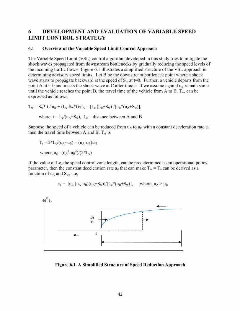
The Variable Speed Limit (VSL) control algorithm developed in this study tries to mitigate the shock waves propagated from downstream bottlenecks by gradually reducing the speed levels of the incoming traffic flows. Figure 6.1 illustrates a simplified structure of the VSL approach in determining advisory speed limits. Let B be the downstream bottleneck point where a shock wave starts to propagate backward at the speed of Sw at t=0. Further, a vehicle departs from the point A at t=0 and meets the shock wave at C after time t. If we assume uA and uB remain same until the vehicle reaches the point B, the travel time of the vehicle from A to B, Tw, can be expressed as follows:
Tw = Sw* t / uB + (Lc-Sw*t)/uA = [Lc (uB+Sw)]/[uB*(uA+Sw)],
where, t = Lc/(uA+Sw), Lc = distance between A and B
Suppose the speed of a vehicle can be reduced from uA to uB with a constant deceleration rate ad, then the travel time between A and B, Ta, is
Ta = 2*Lc/(uA+uB) = (uA-uB)/ad
where, ad =(uA2-uB
2)/(2*Lc)
If the value of Lc, the speed control zone length, can be predetermined as an operational policy parameter, then the constant deceleration rate ad that can make Tw = Ta can be derived as a function of uA and Sw, i..e,
ad = [uB (uA-uB)(uA+Sw)]/[Lc*(uB+Sw)], where, uA > uB
Figure 6.1. A Simplified Structure of Speed Reduction Approach
S
S911
66th
St
43
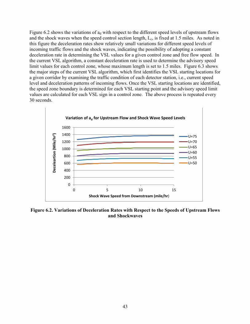
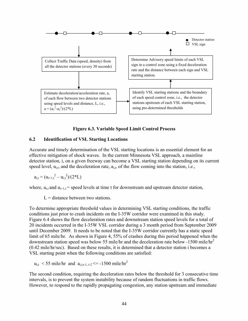
Figure 6.2 shows the variations of ad with respect to the different speed levels of upstream flows and the shock waves when the speed control section length, Lc, is fixed at 1.5 miles. As noted in this figure the deceleration rates show relatively small variations for different speed levels of incoming traffic flows and the shock waves, indicating the possibility of adopting a constant deceleration rate in determining the VSL values for a given control zone and free flow speed. In the current VSL algorithm, a constant deceleration rate is used to determine the advisory speed limit values for each control zone, whose maximum length is set to 1.5 miles. Figure 6.3 shows the major steps of the current VSL algorithm, which first identifies the VSL starting locations for a given corridor by examining the traffic condition of each detector station, i.e., current speed level and deceleration patterns of incoming flows. Once the VSL starting locations are identified, the speed zone boundary is determined for each VSL starting point and the advisory speed limit values are calculated for each VSL sign in a control zone. The above process is repeated every 30 seconds.
Figure 6.2. Variations of Deceleration Rates with Respect to the Speeds of Upstream Flows and Shockwaves
0
200
400
600
800
1000
1200
1400
1600
0 5 10 15
U=75U=70U=65U=60U=55U=50
Variation of ad for Upstream Flow and Shock Wave Speed Levels
Shock Wave Speed from Downstream (mile/hr)
Dece
lear
tion
(Mile
/hr2 )
44
Figure 6.3. Variable Speed Limit Control Process
Collect Traffic Data (speed, density) from all the detector stations (every 30 seconds)
Determine Advisory speed limits of each VSL sign in a control zone using a fixed deceleration rate and the distance between each sign and VSL starting station.
Estimate deceleration/acceleration rate, a, of each flow between two detector stations using speed levels and distance, L, i.e., a = (u1
2-u22)/(2*L)
Identify VSL starting stations and the boundary of each speed control zone, i.e., the detector stations upstream of each VSL starting station, using pre-determined thresholds
Detector station VSL sign
6.2 Identification of VSL Starting Locations
Accurate and timely determination of the VSL starting locations is an essential element for an effective mitigation of shock waves. In the current Minnesota VSL approach, a mainline detector station, i, on a given freeway can become a VSL starting station depending on its current speed level, ui,t, and the deceleration rate, ai,t, of the flow coming into the station, i.e.,
ai,t = (ui+1,t2 – ui,t
2)/(2*L)
where, ui,t and ui+1,t = speed levels at time t for downstream and upstream detector station,
L = distance between two stations.
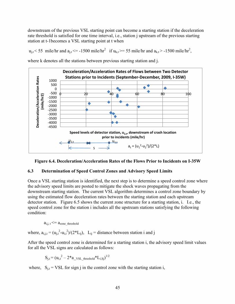
To determine appropriate threshold values in determining VSL starting conditions, the traffic conditions just prior to crash incidents on the I-35W corridor were examined in this study. Figure 6.4 shows the flow deceleration rates and downstream station speed levels for a total of 20 incidents occurred in the I-35W VSL corridor during a 3 month period from September 2009 until December 2009. It needs to be noted that the I-35W corridor currently has a static speed limit of 65 mile/hr. As shown in Figure 4, 55% of crashes during this period happened when the downstream station speed was below 55 mile/hr and the deceleration rate below -1500 mile/hr2 (0.42 mile/hr/sec). Based on these results, it is determined that a detector station i becomes a VSL starting point when the following conditions are satisfied:
ui,t < 55 mile/hr and ai,t,t-1, t-2 <= -1500 mile/hr2
The second condition, requiring the deceleration rates below the threshold for 3 consecutive time intervals, is to prevent the system instability because of random fluctuations in traffic flows. However, to respond to the rapidly propagating congestion, any station upstream and immediate
45
downstream of the previous VSL starting point can become a starting station if the deceleration rate threshold is satisfied for one time interval, i.e., station j upstream of the previous starting station at t-1becomes a VSL starting point at t when
uj,t < 55 mile/hr and aj,t <= -1500 mile/hr2 if uk,t >= 55 mile/hr and ak,t > -1500 mile/hr2,
where k denotes all the stations between previous starting station and j.
Figure 6.4. Deceleration/Acceleration Rates of the Flows Prior to Incidents on I-35W
-4500-4000-3500-3000-2500-2000-1500-1000
-5000
5001000
0 20 40 60 80 100
Decceleration/Acceleration Rates of Flows between Two Detector Stations prior to Incidents (September-December, 2009, I-35W)
Speed levels of detector station, u2,t, downstream of crash location
Dece
lera
tion/
Acce
lera
tion
Rate
s (m
ile/h
r2)
6.3 Determination of Speed Control Zones and Advisory Speed Limits
Once a VSL starting station is identified, the next step is to determine a speed control zone where the advisory speed limits are posted to mitigate the shock waves propagating from the downstream starting station. The current VSL algorithm determines a control zone boundary by using the estimated flow deceleration rates between the starting station and each upstream detector station. Figure 6.5 shows the current zone structure for a starting station, i. I.e., the speed control zone for the station i includes all the upstream stations satisfying the following condition:
ai,j, t <= azone_threshold
where, ai,j,t = (uj,t2-ui,t
2)/(2*Lij), Lij = distance between station i and j
After the speed control zone is determined for a starting station i, the advisory speed limit values for all the VSL signs are calculated as follows:
Sj,t = (ui,t2 – 2*a_VSL_threshold*Li,Sj)1/2
where, Sj,t = VSL for sign j in the control zone with the starting station i,
prior to incidents (mile/hr) u1,t u2,t
at = (u12-u2
2)/(2*L) S
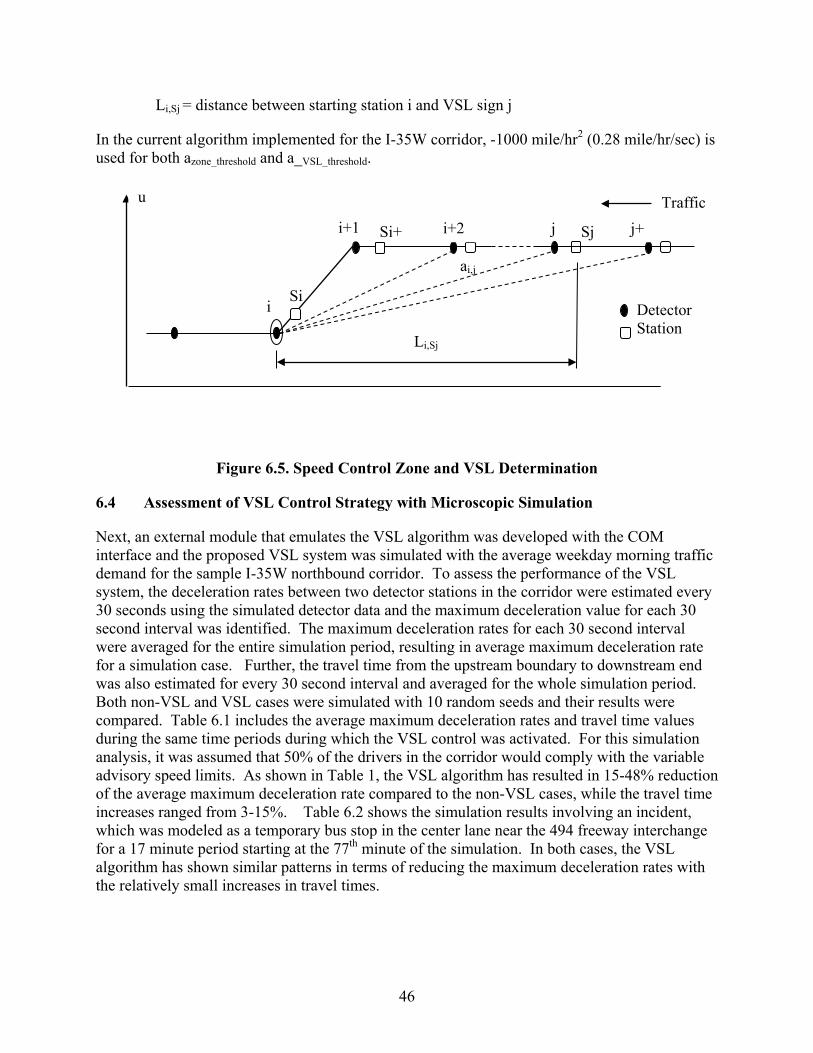
46
Li,Sj = distance between starting station i and VSL sign j
In the current algorithm implemented for the I-35W corridor, -1000 mile/hr2 (0.28 mile/hr/sec) is used for both azone_threshold and a_VSL_threshold.
u
Figure 6.5. Speed Control Zone and VSL Determination
6.4 Assessment of VSL Control Strategy with Microscopic Simulation
Next, an external module that emulates the VSL algorithm was developed with the COM interface and the proposed VSL system was simulated with the average weekday morning traffic demand for the sample I-35W northbound corridor. To assess the performance of the VSL system, the deceleration rates between two detector stations in the corridor were estimated every 30 seconds using the simulated detector data and the maximum deceleration value for each 30 second interval was identified. The maximum deceleration rates for each 30 second interval were averaged for the entire simulation period, resulting in average maximum deceleration rate for a simulation case. Further, the travel time from the upstream boundary to downstream end was also estimated for every 30 second interval and averaged for the whole simulation period. Both non-VSL and VSL cases were simulated with 10 random seeds and their results were compared. Table 6.1 includes the average maximum deceleration rates and travel time values during the same time periods during which the VSL control was activated. For this simulation analysis, it was assumed that 50% of the drivers in the corridor would comply with the variable advisory speed limits. As shown in Table 1, the VSL algorithm has resulted in 15-48% reduction of the average maximum deceleration rate compared to the non-VSL cases, while the travel time increases ranged from 3-15%. Table 6.2 shows the simulation results involving an incident, which was modeled as a temporary bus stop in the center lane near the 494 freeway interchange for a 17 minute period starting at the 77th minute of the simulation. In both cases, the VSL algorithm has shown similar patterns in terms of reducing the maximum deceleration rates with the relatively small increases in travel times.
Sj Si+
Si Detector Station
ai,j
Li,Sj
i
j i+1 i+2 j+
Traffic
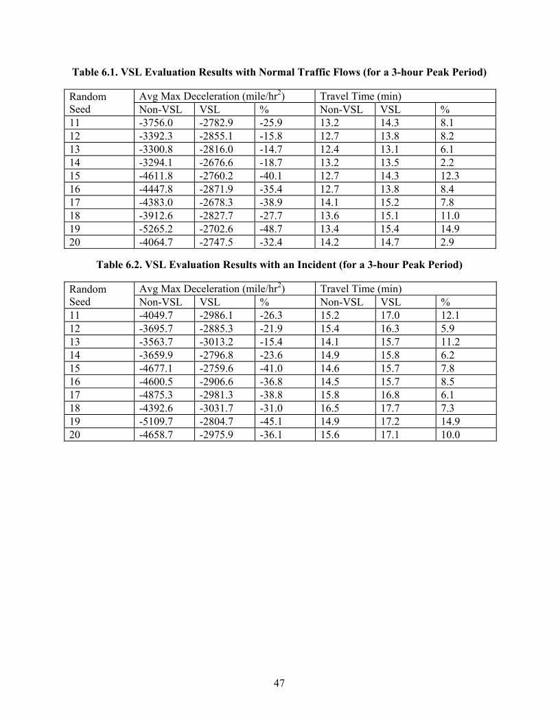
47
Table 6.1. VSL Evaluation Results with Normal Traffic Flows (for a 3-hour Peak Period)
Random Seed
Avg Max Deceleration (mile/hr2) Travel Time (min) Non-VSL VSL % Non-VSL VSL %
11 -3756.0 -2782.9 -25.9 13.2 14.3 8.1 12 -3392.3 -2855.1 -15.8 12.7 13.8 8.2 13 -3300.8 -2816.0 -14.7 12.4 13.1 6.1 14 -3294.1 -2676.6 -18.7 13.2 13.5 2.2 15 -4611.8 -2760.2 -40.1 12.7 14.3 12.3 16 -4447.8 -2871.9 -35.4 12.7 13.8 8.4 17 -4383.0 -2678.3 -38.9 14.1 15.2 7.8 18 -3912.6 -2827.7 -27.7 13.6 15.1 11.0 19 -5265.2 -2702.6 -48.7 13.4 15.4 14.9 20 -4064.7 -2747.5 -32.4 14.2 14.7 2.9
Table 6.2. VSL Evaluation Results with an Incident (for a 3-hour Peak Period)
Random Seed
Avg Max Deceleration (mile/hr2) Travel Time (min) Non-VSL VSL % Non-VSL VSL %
11 -4049.7 -2986.1 -26.3 15.2 17.0 12.1 12 -3695.7 -2885.3 -21.9 15.4 16.3 5.9 13 -3563.7 -3013.2 -15.4 14.1 15.7 11.2 14 -3659.9 -2796.8 -23.6 14.9 15.8 6.2 15 -4677.1 -2759.6 -41.0 14.6 15.7 7.8 16 -4600.5 -2906.6 -36.8 14.5 15.7 8.5 17 -4875.3 -2981.3 -38.8 15.8 16.8 6.1 18 -4392.6 -3031.7 -31.0 16.5 17.7 7.3 19 -5109.7 -2804.7 -45.1 14.9 17.2 14.9 20 -4658.7 -2975.9 -36.1 15.6 17.1 10.0
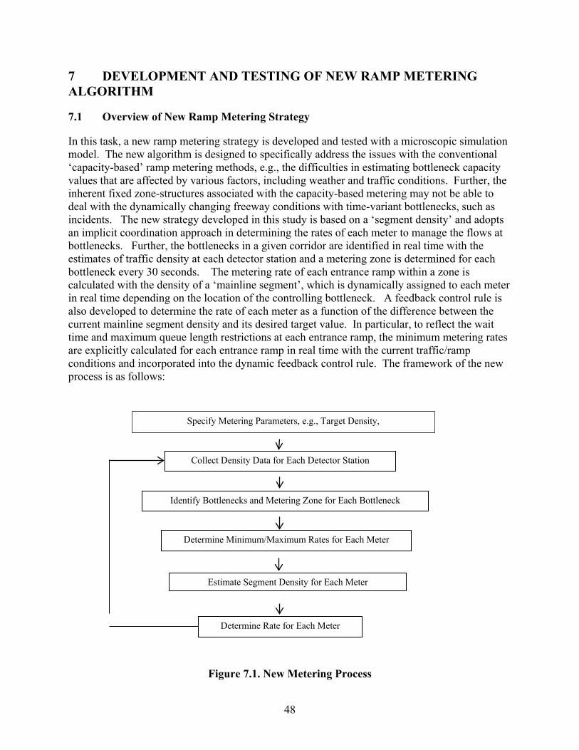
48
7 DEVELOPMENT AND TESTING OF NEW RAMP METERING ALGORITHM
7.1 Overview of New Ramp Metering Strategy
In this task, a new ramp metering strategy is developed and tested with a microscopic simulation model. The new algorithm is designed to specifically address the issues with the conventional ‘capacity-based’ ramp metering methods, e.g., the difficulties in estimating bottleneck capacity values that are affected by various factors, including weather and traffic conditions. Further, the inherent fixed zone-structures associated with the capacity-based metering may not be able to deal with the dynamically changing freeway conditions with time-variant bottlenecks, such as incidents. The new strategy developed in this study is based on a ‘segment density’ and adopts an implicit coordination approach in determining the rates of each meter to manage the flows at bottlenecks. Further, the bottlenecks in a given corridor are identified in real time with the estimates of traffic density at each detector station and a metering zone is determined for each bottleneck every 30 seconds. The metering rate of each entrance ramp within a zone is calculated with the density of a ‘mainline segment’, which is dynamically assigned to each meter in real time depending on the location of the controlling bottleneck. A feedback control rule is also developed to determine the rate of each meter as a function of the difference between the current mainline segment density and its desired target value. In particular, to reflect the wait time and maximum queue length restrictions at each entrance ramp, the minimum metering rates are explicitly calculated for each entrance ramp in real time with the current traffic/ramp conditions and incorporated into the dynamic feedback control rule. The framework of the new process is as follows:
Collect Density Data for Each Detector Station
Identify Bottlenecks and Metering Zone for Each Bottleneck
Determine Minimum/Maximum Rates for Each Meter
Estimate Segment Density for Each Meter
Specify Metering Parameters, e.g., Target Density,
Figure 7.1. New Metering Process
Determine Rate for Each Meter
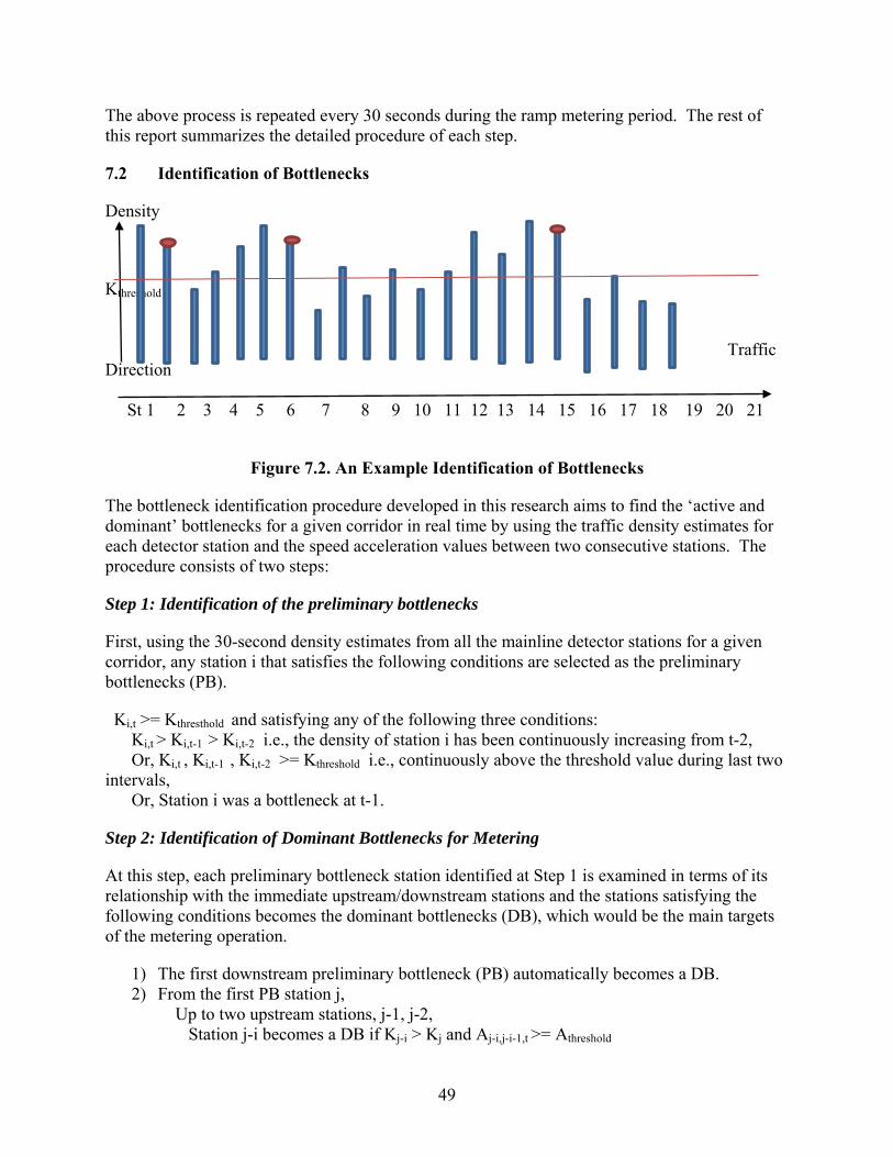
49
The above process is repeated every 30 seconds during the ramp metering period. The rest of this report summarizes the detailed procedure of each step.
7.2 Identification of Bottlenecks
Density
Kthreshold Direction St 1 2
Traffic
3 4 5 6 7 8 9 10 11 12 13 14 15 16 17 18 19 20 21
Figure 7.2. An Example Identification of Bottlenecks
The bottleneck identification procedure developed in this research aims to find the ‘active and dominant’ bottlenecks for a given corridor in real time by using the traffic density estimates for each detector station and the speed acceleration values between two consecutive stations. The procedure consists of two steps:
Step 1: Identification of the preliminary bottlenecks
First, using the 30-second density estimates from all the mainline detector stations for a given corridor, any station i that satisfies the following conditions are selected as the preliminary bottlenecks (PB).
Ki,t >= Kthresthold and satisfying any of the following three conditions: Ki,t > Ki,t-1 > Ki,t-2 i.e., the density of station i has been continuously increasing from t-2, Or, Ki,t , Ki,t-1 , Ki,t-2 >= Kthreshold i.e., continuously above the threshold value during last two intervals, Or, Station i was a bottleneck at t-1.
Step 2: Identification of Dominant Bottlenecks for Metering
At this step, each preliminary bottleneck station identified at Step 1 is examined in terms of its relationship with the immediate upstream/downstream stations and the stations satisfying the following conditions becomes the dominant bottlenecks (DB), which would be the main targets of the metering operation.
1) The first downstream preliminary bottleneck (PB) automatically becomes a DB. 2) From the first PB station j,
Up to two upstream stations, j-1, j-2, Station j-i becomes a DB if Kj-i > Kj and Aj-i,j-i-1,t >= Athreshold
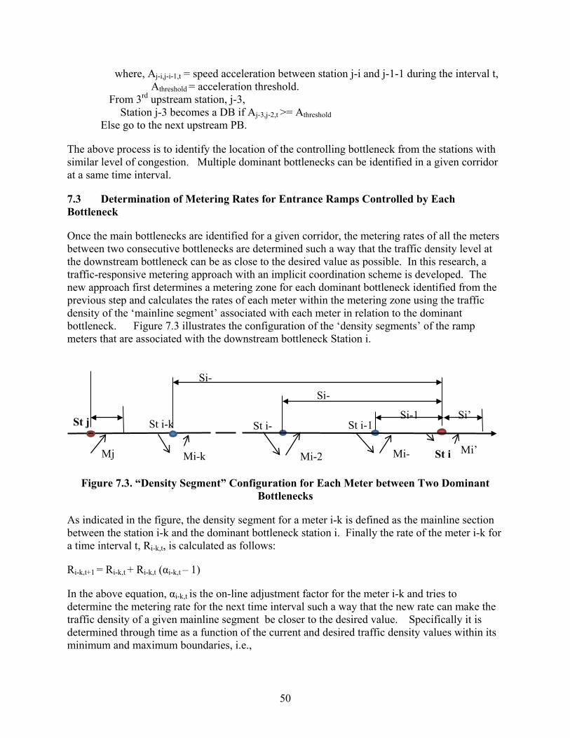
50
where, Aj-i,j-i-1,t = speed acceleration between station j-i and j-1-1 during the interval t, Athreshold = acceleration threshold. From 3rd upstream station, j-3, Station j-3 becomes a DB if Aj-3,j-2,t >= Athreshold Else go to the next upstream PB.
The above process is to identify the location of the controlling bottleneck from the stations with similar level of congestion. Multiple dominant bottlenecks can be identified in a given corridor at a same time interval.
7.3 Determination of Metering Rates for Entrance Ramps Controlled by Each Bottleneck
Once the main bottlenecks are identified for a given corridor, the metering rates of all the meters between two consecutive bottlenecks are determined such a way that the traffic density level at the downstream bottleneck can be as close to the desired value as possible. In this research, a traffic-responsive metering approach with an implicit coordination scheme is developed. The new approach first determines a metering zone for each dominant bottleneck identified from the previous step and calculates the rates of each meter within the metering zone using the traffic density of the ‘mainline segment’ associated with each meter in relation to the dominant bottleneck. Figure 7.3 illustrates the configuration of the ‘density segments’ of the ramp meters that are associated with the downstream bottleneck Station i.
Si’ Si-1
Si-Si-
Mj Mi- Mi’
St j St i-1 St i-St i-k
St i Mi-2 Mi-k
Figure 7.3. “Density Segment” Configuration for Each Meter between Two Dominant Bottlenecks
As indicated in the figure, the density segment for a meter i-k is defined as the mainline section between the station i-k and the dominant bottleneck station i. Finally the rate of the meter i-k for a time interval t, Ri-k,t, is calculated as follows:
Ri-k,t+1 = Ri-k,t + Ri-k,t (αi-k,t – 1)
In the above equation, αi-k,t is the on-line adjustment factor for the meter i-k and tries to determine the metering rate for the next time interval such a way that the new rate can make the traffic density of a given mainline segment be closer to the desired value. Specifically it is determined through time as a function of the current and desired traffic density values within its minimum and maximum boundaries, i.e.,

51
[Ri-k,min,t/Ri-k,t] <= αi-k,t = [Ri-k,max,t/Ri-k,t]
where,
Ri-k,min, t = Minimum rate for the meter i-k for time t,
Ri-k, max,t = Maximum rate for the meter i-k for time t.
Let Ki-k,t = Average traffic density for the segment between the bottleneck Station i and the Station i-k
during time interval t,
Ki-k,d = Desired traffic density for the segment between the station i and i-k,
Figure 7.3.2 shows the process to determine αi-k,t as a function of the difference between the desired and current values of a given segment. In Figure 7.3.2, the segment density, Ki-k,t, is calculated as an weighted average of all the station densities between station i and i-k, i.e.,
Ki-k,t = Σ [(ki-j,t i/3) + (ki-j,t + ki-j+1,t)/6 + (ki-j+1,t / 3)]*Li-j,i-j+1 /Li-k,i
where, Li-k,i = Distance between stations i-k and i.
The above procedure tries to improve the mainline segment density by implicitly coordinating the multiple ramps affected by a same bottleneck, while the current restrictions on maximum wait time limit are explicitly incorporated into the metering rate calculation process.
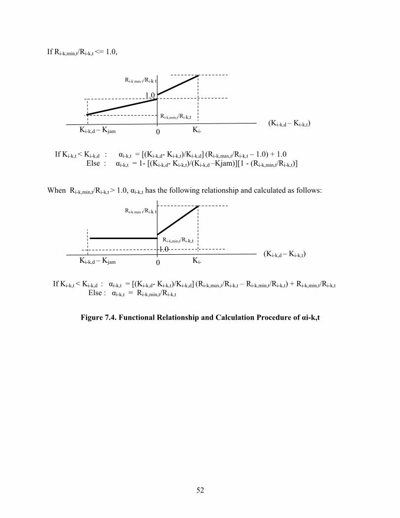
52
If Ri-k,min,t/Ri-k,t <= 1.0,
If Ki-k,t < Ki-k,d : αi-k,t = [(Ki-k,d- Ki-k,t)/Ki-k,d] (Ri-k,max,t/Ri-k,t – 1.0) + 1.0 Else : αi-k,t = 1- [(Ki-k,d- Ki-k,t)/(Ki-k,d –Kjam)][1 - (Ri-k,min,t/Ri-k,t)] When Ri-k,min,t/Ri-k,t > 1.0, αi-k,t has the following relationship and calculated as follows:
Ki-k,d – Kjam
αi-
0
1.0
Ki-k,d – Kjam Ki-
Ri-k,min,t/Ri-k,t
Ri-k max t/Ri-k t
(Ki-k,d – Ki-k,t)
0
1.0 Ki-
Ri-k,min,t/Ri-k,t
Ri-k max t/Ri-k t
(Ki-k,d – Ki-k,t)
If Ki-k,t < Ki-k,d : αi-k,t = [(Ki-k,d- Ki-k,t)/Ki-k,d] (Ri-k,max,t/Ri-k,t – Ri-k,min,t/Ri-k,t) + Ri-k,min,t/Ri-k,t Else : αi-k,t = Ri-k,min,t/Ri-k,t
Figure 7.4. Functional Relationship and Calculation Procedure of αi-k,t
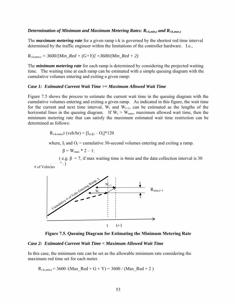
53
Determination of Minimum and Maximum Metering Rates: Ri-k,min,t and Ri-k,max,t
The maximum metering rate for a given ramp i-k is governed by the shortest red time interval determined by the traffic engineer within the limitations of the controller hardware. I.e.,
Ri-k,max,t = 3600/[Min_Red + (G+Y)] =3600/(Min_Red + 2)
The minimum metering rate for each ramp is determined by considering the projected waiting time. The waiting time at each ramp can be estimated with a simple queuing diagram with the cumulative volumes entering and exiting a given ramp:
Case 1: Estimated Current Wait Time >= Maximum Allowed Wait Time
Figure 7.5 shows the process to estimate the current wait time in the queuing diagram with the cumulative volumes entering and exiting a given ramp. As indicated in this figure, the wait time for the current and next time interval, Wt and Wt+1, can be estimated as the lengths of the horizontal lines in the queuing diagram. If Wt > Wmax, maximum allowed wait time, then the minimum metering rate that can satisfy the maximum estimated wait time restriction can be determined as follows:
Ri-k,min,t (veh/hr) = [I(t-β) – Ot]*120
where, It and Ot = cumulative 30-second volumes entering and exiting a ramp.
β = Wmax * 2 – 1:
( e.g. β = 7, if max waiting time is 4min and the data collection interval is 30 seconds )
Cumulative # of Vehs exiting Ramp, Ot
Wt+1
Wt Rmin,t+1
Figure 7.5. Queuing Diagram for Estimating the Minimum Metering Rate
Case 2: Estimated Current Wait Time < Maximum Allowed Wait Time
In this case, the minimum rate can be set as the allowable minimum rate considering the maximum red time set for each meter.
Ri-k,min,t = 3600 /(Max_Red + G + Y) = 3600 / (Max_Red + 2 )
t t+1
# of Vehicles
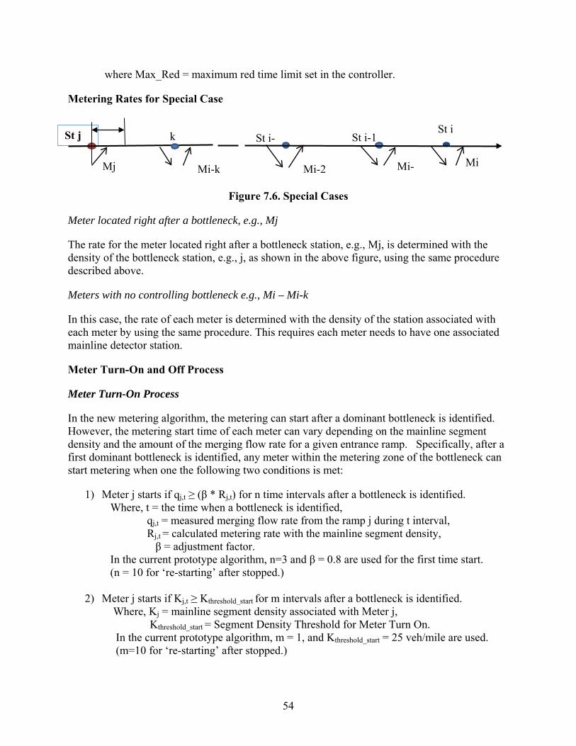
54
where Max_Red = maximum red time limit set in the controller.
Metering Rates for Special Case
St j
Mj
St i-
Figure 7.6. Special Cases
Mi- Mi
St i-1 St i-St i
Mi-2
k
Mi-k
Meter located right after a bottleneck, e.g., Mj
The rate for the meter located right after a bottleneck station, e.g., Mj, is determined with the density of the bottleneck station, e.g., j, as shown in the above figure, using the same procedure described above.
Meters with no controlling bottleneck e.g., Mi – Mi-k
In this case, the rate of each meter is determined with the density of the station associated with each meter by using the same procedure. This requires each meter needs to have one associated mainline detector station.
Meter Turn-On and Off Process
Meter Turn-On Process
In the new metering algorithm, the metering can start after a dominant bottleneck is identified. However, the metering start time of each meter can vary depending on the mainline segment density and the amount of the merging flow rate for a given entrance ramp. Specifically, after a first dominant bottleneck is identified, any meter within the metering zone of the bottleneck can start metering when one the following two conditions is met:
1) Meter j starts if qj,t ≥ (β * Rj,t) for n time intervals after a bottleneck is identified. Where, t = the time when a bottleneck is identified, qj,t = measured merging flow rate from the ramp j during t interval, Rj,t = calculated metering rate with the mainline segment density, β = adjustment factor. In the current prototype algorithm, n=3 and β = 0.8 are used for the first time start. (n = 10 for ‘re-starting’ after stopped.)
2) Meter j starts if Kj,t ≥ Kthreshold_start for m intervals after a bottleneck is identified. Where, Kj = mainline segment density associated with Meter j, Kthreshold_start = Segment Density Threshold for Meter Turn On. In the current prototype algorithm, m = 1, and Kthreshold_start = 25 veh/mile are used. (m=10 for ‘re-starting’ after stopped.)

55
Meter Turn-Off Process
Case 1: Meters downstream of the last bottleneck, i.e., no further downstream bottleneck
For a meter downstream of the last bottleneck, if all of the following 3 conditions are satisfied for n time intervals: (the metering rate, Ri,t, for the ramp i is calculated with the local segment density).
1) qi,t ≤ Ri,t, 2) Ki,t ≤ Kd 3) No new bottleneck downstream of the ramp i
Current prototype algorithm: n = 5 minutes.
Case 2: For the ramps upstream of a bottleneck : when only one bottleneck is left.
The turn-off process is activated for the ramps located upstream of the last bottlenck when the average density of the entire segment upstream of the last bottleneck continuously decreases or does not increase for the last n time intervals, i.e,.
Kt ≤ ≤ ≤ ≤ Kt-n, and only one bottleneck is left,
where Kt-i = 15 min moving average of the weighted average density for the segment between the last bottleneck and the most upstream station in a given corridor at t-i time interval.
The turn-off process consists of two steps:
Step 1: Change the bottleneck threshold density: i.e, for a station to become a preliminary bottleneck, the station density needs to be greater than Kthreshold_after for n previous intervals. Currently Kthreshold_after = 32 veh/mile, and n=2 minutes are used.
Step 2: Check each ramp upstream of the bottleneck: the ramp i upstream of the bottleneck can stop metering if the following two conditions are met:
1) qi,t ≤ Ri,t and 2) Ki,t, Ki,t-1, ----- Ki,t-n ≤ Kd where, qi,t = measured merging flow rate of ramp i, at t, Ri,t = caculated metering rate for ramp i at t, Ki,t-k = Segment density for ramp i at t-k, Kd = desired density Currently n=5 minutes, and Kd = 0.8 * critical density
Metering restart condtion
The new algorithm allows for a meter j to restart metering under the following conditions:
Kj,t ≥ Kthreshold_after and qj,t ≥ (β * Rj,t) for n time intervals. Currently n=5 minutes, and β = 0.8.
The above condition is more restrictive than the requirements in the initial turn-on process to avoid unncessary metering from the random fluctuations in the traffic flow.
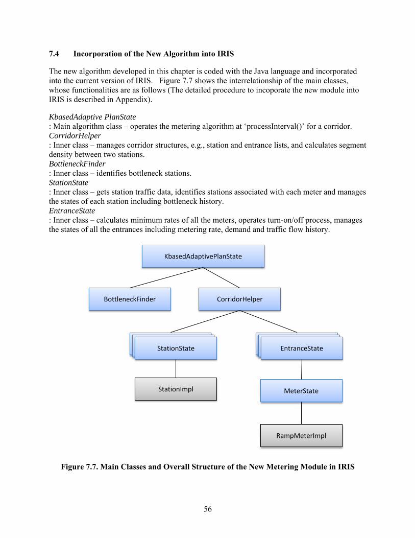
56
7.4 Incorporation of the New Algorithm into IRIS
The new algorithm developed in this chapter is coded with the Java language and incorporated into the current version of IRIS. Figure 7.7 shows the interrelationship of the main classes, whose functionalities are as follows (The detailed procedure to incoporate the new module into IRIS is described in Appendix).
KbasedAdaptive PlanState : Main algorithm class – operates the metering algorithm at ‘processInterval()’ for a corridor. CorridorHelper : Inner class – manages corridor structures, e.g., station and entrance lists, and calculates segment density between two stations. BottleneckFinder : Inner class – identifies bottleneck stations. StationState : Inner class – gets station traffic data, identifies stations associated with each meter and manages the states of each station including bottleneck history. EntranceState : Inner class – calculates minimum rates of all the meters, operates turn-on/off process, manages the states of all the entrances including metering rate, demand and traffic flow history.
Figure 7.7. Main Classes and Overall Structure of the New Metering Module in IRIS
KbasedAdaptivePlanState
BottleneckFinder CorridorHelper
StationState EntranceState
MeterState
StationState StationState EntranceState EntranceState
RampMeterImpl
StationImpl
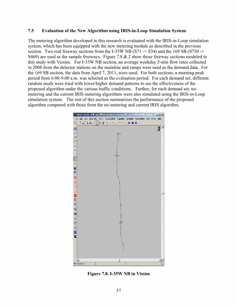
57
7.5 Evaluation of the New Algorithm using IRIS-in-Loop Simulation System
The metering algorithm developed in this research is evaluated with the IRIS-in-Loop simulation system, which has been equipped with the new metering module as described in the previous section. Two real freeway sections from the I-35W NB (S71 -> S34) and the 169 SB (S750 -> S469) are used as the sample freeways. Figure 7.8 & 2 show those freeway sections modeled in this study with Vissim. For I-35W NB section, an average weekday 5-min flow rates collected in 2008 from the detector stations on the mainline and ramps were used as the demand data. For the 169 SB section, the data from April 7, 2011, were used. For both sections, a morning peak period from 6:00-9:00 a.m. was selected as the evaluation period. For each demand set, different random seeds were tried with lower/higher demand patterns to see the effectiveness of the proposed algorithm under the various traffic conditions. Further, for each demand set, no-metering and the current IRIS metering algorithms were also simulated using the IRIS-in-Loop simulation system. The rest of this section summarizes the performance of the proposed algorithm compared with those from the no-metering and current IRIS algorithm.
Figure 7.8. I-35W NB in Vissim
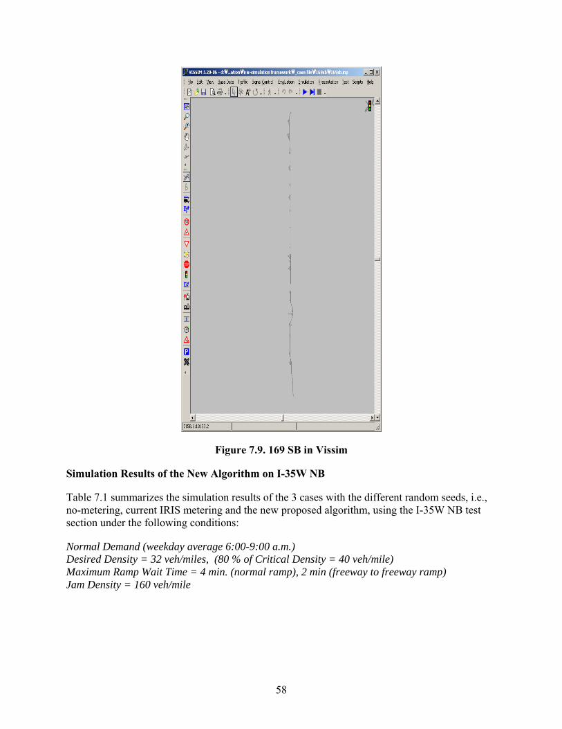
58
Figure 7.9. 169 SB in Vissim
Simulation Results of the New Algorithm on I-35W NB
Table 7.1 summarizes the simulation results of the 3 cases with the different random seeds, i.e., no-metering, current IRIS metering and the new proposed algorithm, using the I-35W NB test section under the following conditions:
Normal Demand (weekday average 6:00-9:00 a.m.) Desired Density = 32 veh/miles, (80 % of Critical Density = 40 veh/mile) Maximum Ramp Wait Time = 4 min. (normal ramp), 2 min (freeway to freeway ramp) Jam Density = 160 veh/mile
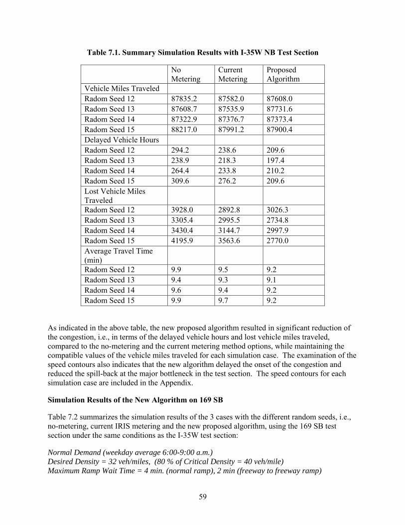
59
Table 7.1. Summary Simulation Results with I-35W NB Test Section
No Metering
Current Metering
Proposed Algorithm
Vehicle Miles Traveled Radom Seed 12 87835.2 87582.0 87608.0 Radom Seed 13 87608.7 87535.9 87731.6 Radom Seed 14 87322.9 87376.7 87373.4 Radom Seed 15 88217.0 87991.2 87900.4 Delayed Vehicle Hours Radom Seed 12 294.2 238.6 209.6 Radom Seed 13 238.9 218.3 197.4 Radom Seed 14 264.4 233.8 210.2 Radom Seed 15 309.6 276.2 209.6 Lost Vehicle Miles Traveled
Radom Seed 12 3928.0 2892.8 3026.3 Radom Seed 13 3305.4 2995.5 2734.8 Radom Seed 14 3430.4 3144.7 2997.9 Radom Seed 15 4195.9 3563.6 2770.0 Average Travel Time (min)
Radom Seed 12 9.9 9.5 9.2 Radom Seed 13 9.4 9.3 9.1 Radom Seed 14 9.6 9.4 9.2 Radom Seed 15 9.9 9.7 9.2
As indicated in the above table, the new proposed algorithm resulted in significant reduction of the congestion, i.e., in terms of the delayed vehicle hours and lost vehicle miles traveled, compared to the no-metering and the current metering method options, while maintaining the compatible values of the vehicle miles traveled for each simulation case. The examination of the speed contours also indicates that the new algorithm delayed the onset of the congestion and reduced the spill-back at the major bottleneck in the test section. The speed contours for each simulation case are included in the Appendix.
Simulation Results of the New Algorithm on 169 SB
Table 7.2 summarizes the simulation results of the 3 cases with the different random seeds, i.e., no-metering, current IRIS metering and the new proposed algorithm, using the 169 SB test section under the same conditions as the I-35W test section:
Normal Demand (weekday average 6:00-9:00 a.m.) Desired Density = 32 veh/miles, (80 % of Critical Density = 40 veh/mile) Maximum Ramp Wait Time = 4 min. (normal ramp), 2 min (freeway to freeway ramp)
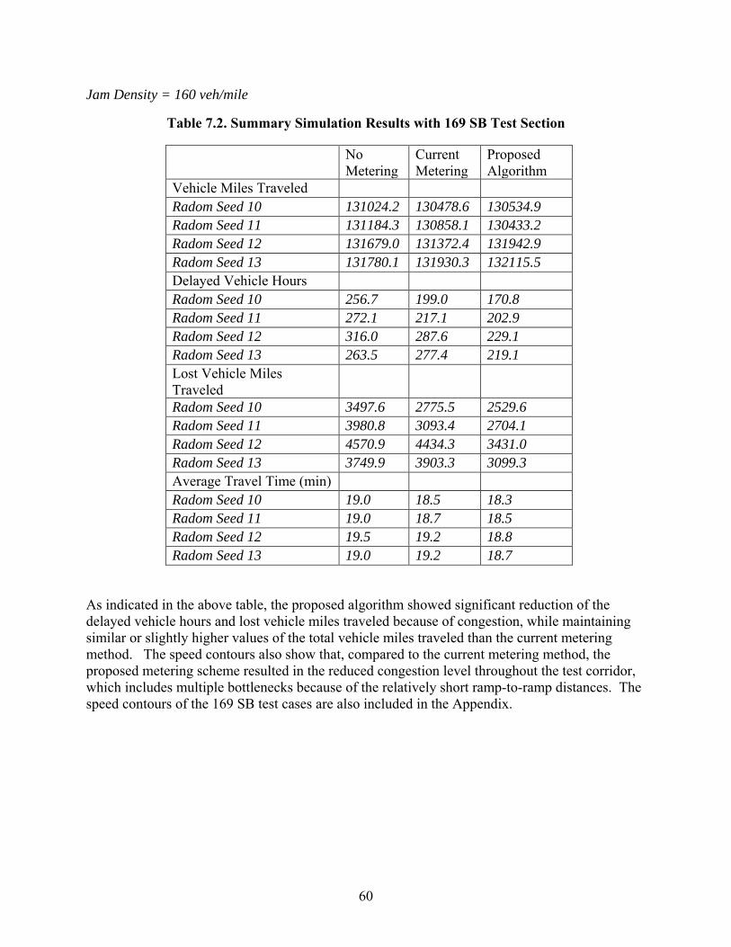
60
Jam Density = 160 veh/mile
Table 7.2. Summary Simulation Results with 169 SB Test Section
No Metering
Current Metering
Proposed Algorithm
Vehicle Miles Traveled Radom Seed 10 131024.2 130478.6 130534.9 Radom Seed 11 131184.3 130858.1 130433.2 Radom Seed 12 131679.0 131372.4 131942.9 Radom Seed 13 131780.1 131930.3 132115.5 Delayed Vehicle Hours Radom Seed 10 256.7 199.0 170.8 Radom Seed 11 272.1 217.1 202.9 Radom Seed 12 316.0 287.6 229.1 Radom Seed 13 263.5 277.4 219.1 Lost Vehicle Miles Traveled
Radom Seed 10 3497.6 2775.5 2529.6 Radom Seed 11 3980.8 3093.4 2704.1 Radom Seed 12 4570.9 4434.3 3431.0 Radom Seed 13 3749.9 3903.3 3099.3 Average Travel Time (min) Radom Seed 10 19.0 18.5 18.3 Radom Seed 11 19.0 18.7 18.5 Radom Seed 12 19.5 19.2 18.8 Radom Seed 13 19.0 19.2 18.7
As indicated in the above table, the proposed algorithm showed significant reduction of the delayed vehicle hours and lost vehicle miles traveled because of congestion, while maintaining similar or slightly higher values of the total vehicle miles traveled than the current metering method. The speed contours also show that, compared to the current metering method, the proposed metering scheme resulted in the reduced congestion level throughout the test corridor, which includes multiple bottlenecks because of the relatively short ramp-to-ramp distances. The speed contours of the 169 SB test cases are also included in the Appendix.
61
8 CONCLUSIONS
This research produced several important tools that are essential in managing and operating freeway corridors. First, an off-line process and a computer program were developed to automatically estimate the performance of a given freeway corridor for selected time periods using the data collected from the existing detectors on the field. Further, a set of traffic measures were developed and incorporated into the software, called TICAS (Traffic Information and Condition Analysis System), whose built-in contour module provides a graphical overview of the traffic parameter variation process through time and space. Using the contour module, the location of bottlenecks and their effects can be easily identified for a given corridor during the selected time periods. Secondly, an on-line process was developed to estimate the selected performance measures using the current day traffic data in real time. The on-line process was designed to assist traffic operators in monitoring the current day traffic trends and identifying any abnormal patterns.
Third, an integrated simulation system was developed by combining IRIS, the freeway traffic control system developed by MnDOT, and the Vissim microscopic simulation software, so that new operational strategies can be directly coded into IRIS and evaluated under the simulated environment. The resulting IRIS-in-Loop Simulation System (ILSS) makes it possible to develop realistic operational strategies that can directly work under the current freeway operational environment. The ILSS was applied to assess two new operational strategies developed in this study: Variable Advisory Speed Limit Control and Density-based Adaptive Metering Strategies. The new variable advisory speed limit control strategy is designed to mitigate the shock waves propagated from downstream bottlenecks by gradually reducing the speed levels of the incoming traffic flows. The algorithm first identifies the locations of the bottlenecks and the VSL control zones by examining the flow deceleration rates between two detector stations in a given corridor. The advisory speed limits for each control zone are calculated with a constant deceleration rate, which has been determined to result in minimum increases in travel times. The relatively simple procedures of the proposed VSL approach, which determines bottleneck locations and advisory speed limit values with the data from the existing loop detectors, can be easily transferrable to most operational environments. The preliminary evaluation results with microscopic simulation indicate that the proposed VSL system could significantly reduce the sudden deceleration rates of the traffic flows reacting to fixed or moving bottlenecks, while the increases in travel times can be kept relatively small. The variable speed limit control strategy has been implemented at the I-35W corridor in July 2010 and the detailed analysis of the field data will be conducted in a subsequent phase of this research.
Finally, an alternative ramp metering algorithm was developed and evaluated with ILSS. The new algorithm identifies bottlenecks for a given corridor every 30 seconds and determines the metering rates for each entrance ramp with the estimated mainline ‘segment density’. Further, the ramp wait time restriction is explicitly incorporated into the metering rate calculation. The new algorithm was simulated with ILSS using two real corridors, I-35W NB and 169 SB, and its performance was compared with those from the current IRIS metering control and No-metering cases. The simulation results indicate substantial improvements over the existing control method in terms of reducing congestion, such as delayed vehicle hours and lost vehicle miles traveled, while achieving the similar levels of vehicle miles traveled.

62
Future research needs include the field testing of the proposed ramp metering strategy on a selected corridor. Further, the variable speed limit control algorithm can be enhanced to reflect different weather conditions and also to reduce the bottleneck identification time. The development of the on-line prediction capability for the traffic flow parameters by extending the current on/off-line estimation process is also recommended as the major step toward proactive traffic management.
63
REFERENCES
1. MnDOT, Intelligent Roadway Information System (IRIS) User Manual, Regional Transportation Management Center, Minnesota Department of Transportation, St. Paul, MN, 2008.
2. Kwon, E., Ambadipudi, R. and Bieniek, J. “Adaptive Coordination of Ramp Meter and Intersection Signal for Balanced Management of a Freeway Corridor”, Compendium of Papers, 2005 Annual Transportation Research Board Meeting, Washington, D.C., January 2005.
3. Kwon, E., Nanduri, S., Lau, R. and Aswegan, J., “Comparative analysis of operational algorithms for coordinated ramp metering”, Transportation Research Record, 1748, pp. 144-152, 2001.
4. PTV, Vissim 5.3 User Manual, 2011.

APPENDIX A. PROCESS TO INCORPORATE NEW METERING ALGORITHM INTO IRIS
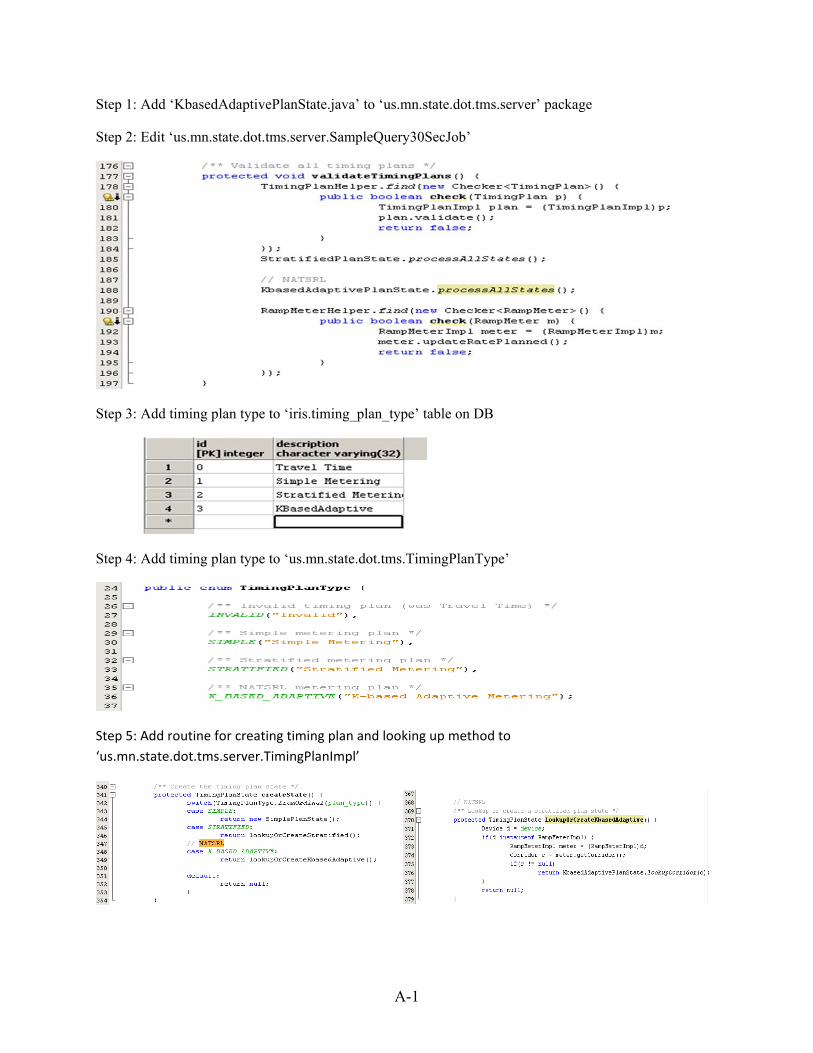
A-1
Step 1: Add ‘KbasedAdaptivePlanState.java’ to ‘us.mn.state.dot.tms.server’ package
Step 2: Edit ‘us.mn.state.dot.tms.server.SampleQuery30SecJob’
Step 3: Add timing plan type to ‘iris.timing_plan_type’ table on DB
Step 4: Add timing plan type to ‘us.mn.state.dot.tms.TimingPlanType’
Step 5: Add routine for creating timing plan and looking up method to
‘us.mn.state.dot.tms.server.TimingPlanImpl’

APPENDIX B. SPEED CONTOURS FROM SIMULATION RESULTS
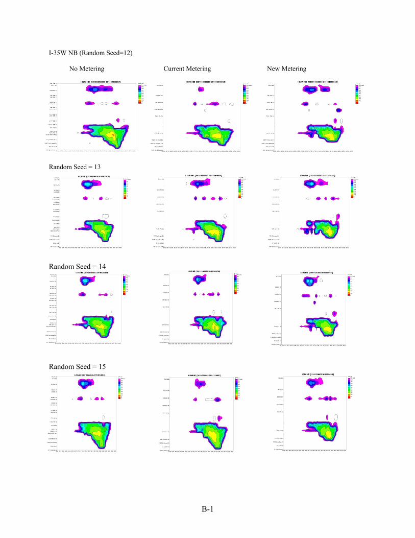
B-1
I-35W NB (Random Seed=12)
No Metering Current Metering New Metering
Random Seed = 13
Random Seed = 14
Random Seed = 15
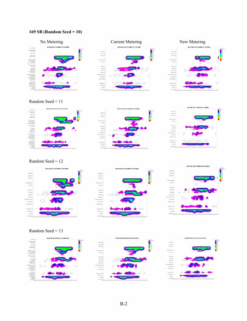
B-2
169 SB (Random Seed = 10)
No Metering Current Metering New Metering
Random Seed = 11
Random Seed = 12
Random Seed = 13