Embed Size (px)
Citation preview
UNIVERSIDADE FEDERAL DE MINAS GERAISSCHOOL OF ENGINEERING
UNDERGRADUATE COURSE IN AEROSPACE ENGINEERING
ARTHUR HENRIQUES LORENTZ GODINHO AMARAL
DEVELOPMENT OF FAST ANALYTICAL METHODS FOR THERECONSTRUCTION OF 3D SHOCK STRUCTURES
GENERATED BY BODIES TRAVELING AT SUPERSONIC ANDHYPERSONIC SPEEDS
Belo Horizonte2018
UNIVERSIDADE FEDERAL DE MINAS GERAISSCHOOL OF ENGINEERING
UNDERGRADUATE COURSE IN AEROSPACE ENGINEERING
ARTHUR HENRIQUES LORENTZ GODINHO AMARAL
DEVELOPMENT OF FAST ANALYTICAL METHODS FOR THERECONSTRUCTION OF 3D SHOCK STRUCTURES
GENERATED BY BODIES TRAVELING AT SUPERSONIC ANDHYPERSONIC SPEEDS
Undergraduate thesis submitted in partial ful-filment of the requirements for the degree ofBachelor in Aerospace Engineering
Supervisor: Prof. Dr. Guilherme de Souza Papini
Belo Horizonte2018

Henriques Lorentz Godinho Amaral, ArthurDEVELOPMENT OF FAST ANALYTICAL METHODS FOR THE RECONSTRUC-
TION OF 3D SHOCK STRUCTURES GENERATED BY BODIES TRAVELING ATSUPERSONIC AND HYPERSONIC SPEEDS/ ARTHUR HENRIQUES LORENTZGODINHO AMARAL. – Belo Horizonte, 2018.
70 p. : il. (algumas color.) ; 30 cm.
Supervisor: Prof. Dr. Guilherme de Souza Papini
Undergraduate Thesis – UNIVERSIDADE FEDERAL DE MINAS GERAISSCHOOL OF ENGINEERINGUNDERGRADUATE COURSE IN AEROSPACE ENGINEERING, 2018.1. Hypersonic flow. 2. Shock structure prediction. 3. Preliminary design.

ACKNOWLEDGEMENTS
This work could not have been accomplished without the trust of my supervisors, Dr.Romain Wuilbercq, who believed its success from the very first day; and Dr. Guilherme Papinifor his full support since my return.
I extend my deepest appreciation to ONERA for giving me this opportunity, to LJLL forhaving received me so well, and to ISAE-ENSMA which is where this journey began.
I would like to thank my parents, Álvaro and Giselle, for their unconditional supportthroughout my life. 9000 kilometers were not enough to stop them from being the best.
I would also like to thank my brother, Pedro, for the midnight bursts of laughter and forteaching me the fine art of destroying my own creations to make them better, developing a senseof continuous improvement.
I cannot thank enough my friends in Brazil that helped me feel at home and never forgetwhere I come from; and my friends in Europe, who gave me a new home along with a Spanishand Italian heart.

“I soon discovered that them expecting me to be able to do it made me able to do it. None of it is
really rocket science. It’s not like this secret skill. The power of somebody to set up a situation
where you feel there is no question you can fulfill an expectation is very powerful.”
ABSTRACT
The purpose of this research is to develop a preliminary design tool for shock structure predictionin supersonic and hypersonic flows supported by the available bibliography, identifying theinherent problems and improvement opportunities. Despite the phenomena involved in thoseflow regimes which interact among themselves in complex ways, simplified inviscid modelsare employed in a combination of analytical and empirical methods to obtain low-fidelity, high-credibility solutions. A review of the underlying concepts and assumptions that support thesemodels is also presented. Computational costs and robustness are given high priority with thegoal of a future optimization application. The model is initially two-dimensional and is graduallybuilt upon to achieve a three-dimensional method. The results obtained with sample bodies arethen analyzed and compared with numerical simulations. As conclusions, perspectives of thepotential of the methodology and avenues for future work are also proposed.
Keywords: hypersonic flow. shock structure prediction. preliminary design.

RESUMO
O propósito desta pesquisa é desenvolver uma ferramenta de anteprojeto para a previsão daestrutura de choques em escoamentos supersônicos e hipersônicos embasada na bibliografiadisponível, identificando os problemas inerentes e oportunidades de melhoria. Apesar dosfenômenos envolvidos nesses regimes de escoamento que interagem entre si de formas complexas,modelos invíscidos simplificados são empregados em uma combinação de métodos analíticos eempíricos para obter soluções de baixa fidelidade e alta credibilidade. Uma revisão dos conceitosfundamentais e hipóteses que apoiam os modelos também é apresentada. Custos computacionaise robustez são fortemente priorizados visando uma aplicação em uma otimização futura. Omodelo é inicialmente bidimensional e é desenvolvido gradualmente para obter um métodotridimensional. Os resultados obtidos com corpos de exemplo são analisados e comparadosàs simulações numéricas. Como conclusões, perspectivas sobre o potencial da metodologia epossíveis trabalhos futuros são também propostos.
Palavras-chave: escoamento hipersônico. previsão de estrutura de choque. anteprojeto.

LIST OF FIGURES
Figure 1 – Post-flight conditions of a dummy ramjet engine. . . . . . . . . . . . . . . 16Figure 2 – Depiction of a TSTO vehicle. . . . . . . . . . . . . . . . . . . . . . . . . . 17Figure 3 – Mesh refined around the estimated shock region. . . . . . . . . . . . . . . . 17Figure 4 – Subsonic flow over an airfoil. . . . . . . . . . . . . . . . . . . . . . . . . . 20Figure 5 – Supersonic flow over a wedge. . . . . . . . . . . . . . . . . . . . . . . . . 20Figure 6 – Transonic flow over an airfoil. . . . . . . . . . . . . . . . . . . . . . . . . . 21Figure 7 – Hypersonic flow over a wedge. . . . . . . . . . . . . . . . . . . . . . . . . 22Figure 8 – Attached shock examples. . . . . . . . . . . . . . . . . . . . . . . . . . . . 22Figure 9 – Oblique shock angle relation chart. . . . . . . . . . . . . . . . . . . . . . . 24Figure 10 – Detached shock examples. . . . . . . . . . . . . . . . . . . . . . . . . . . . 24Figure 11 – Taylor-Maccoll cone flow schematic. . . . . . . . . . . . . . . . . . . . . . 25Figure 12 – Illustration of the Tangent-Wedge method. . . . . . . . . . . . . . . . . . . 27Figure 13 – Illustration of the Tangent-Cone method. . . . . . . . . . . . . . . . . . . . 27Figure 14 – Shock-Expansion method. . . . . . . . . . . . . . . . . . . . . . . . . . . . 28Figure 15 – Reflection of expansion waves in different regimes. . . . . . . . . . . . . . 28Figure 16 – Step by step depiction of the attached shock method. . . . . . . . . . . . . . 29Figure 17 – Simple wedge shock examples. . . . . . . . . . . . . . . . . . . . . . . . . 31Figure 18 – Starting procedure for detached shocks. . . . . . . . . . . . . . . . . . . . . 32Figure 19 – A circle that circumscribes a triangle. . . . . . . . . . . . . . . . . . . . . . 33Figure 20 – Detached shocks over cylinders at different Mach numbers. . . . . . . . . . 34Figure 21 – Herrera’s correction factor chart. . . . . . . . . . . . . . . . . . . . . . . . 35Figure 22 – Cylinder examples with and without the correction factor. . . . . . . . . . . 36Figure 23 – New correction factor chart. . . . . . . . . . . . . . . . . . . . . . . . . . . 37Figure 24 – Multiple shock example on a wedge with three slopes. . . . . . . . . . . . . 37Figure 25 – Body segmentation examples. . . . . . . . . . . . . . . . . . . . . . . . . . 39Figure 26 – Attached shock over a compressed Von Karman ogive. . . . . . . . . . . . . 41Figure 27 – Construction of a blunt wedge. . . . . . . . . . . . . . . . . . . . . . . . . 41Figure 28 – Blunt wedge with a 60◦ slope angle at M∞ = 6. . . . . . . . . . . . . . . . . 42Figure 29 – Tri-wedge configuration with a strong expansion fan. . . . . . . . . . . . . 42Figure 30 – A Von Karman ogive followed by a wedge illustrating multi-shock errors. . 43Figure 31 – A first attempt to capture the errors induced by a non-circular subsonic region. 44Figure 32 – Circle-ellipse body simulation before and after radius correction. . . . . . . 45Figure 33 – Simulation over an ellipse. . . . . . . . . . . . . . . . . . . . . . . . . . . 46Figure 34 – Half-Edge structure schematic. . . . . . . . . . . . . . . . . . . . . . . . . 47Figure 35 – Example of an irregular cone surface mesh viewed with Medit. . . . . . . . 49Figure 36 – 2D AABB Tree construction algorithm. . . . . . . . . . . . . . . . . . . . . 50Figure 37 – Generic 3D AABB Tree example. . . . . . . . . . . . . . . . . . . . . . . . 50Figure 38 – Vertex normals of a dodecahedral mesh. . . . . . . . . . . . . . . . . . . . 51

Figure 39 – Streamlines traced over a cone. . . . . . . . . . . . . . . . . . . . . . . . . 52Figure 40 – A generic 3D KD-Tree of a point cloud. . . . . . . . . . . . . . . . . . . . 53Figure 41 – Herrera’s KD-Tree search radius for point elimination. . . . . . . . . . . . . 54Figure 42 – Errors induced by a slightly irregular 2D polyline. . . . . . . . . . . . . . . 56Figure 43 – Convex hull of a very irregular 2D polygon. . . . . . . . . . . . . . . . . . 57Figure 44 – Irregular streamline without 2D convex hull correction. . . . . . . . . . . . 58Figure 45 – Streamline with 2D convex hull correction. . . . . . . . . . . . . . . . . . . 59Figure 46 – 3D Convex hull of a conic shock point cloud. . . . . . . . . . . . . . . . . . 60Figure 47 – Cone shock after re-meshing the 3D convex hull. . . . . . . . . . . . . . . . 60Figure 48 – Cone shock compared to an axisymmetric CFD simulation at M∞ = 7. . . . 61Figure 49 – Modified Von Karman ogive compared to an axisymmetric CFD simulation
at M∞ = 7. . . . . . . . . . . . . . . . . . . . . . . . . . . . . . . . . . . . 62Figure 50 – Modified Von Karman ogive simulation with Shock-Expansion method at
M∞ = 7. . . . . . . . . . . . . . . . . . . . . . . . . . . . . . . . . . . . . 62Figure 51 – Blunt cone shock compared to an axisymmetric CFD simulation at M∞ = 7. 63Figure 52 – Blunt cone shock mesh distorted by irregularities. . . . . . . . . . . . . . . 64

LIST OF ABBREVIATIONS AND ACRONYMS
2D Two-dimensional
3D Three-dimensional
AABB Axis-Aligned Bounding Box
ASCII American Standard Code for Information Interchange
CFD Computational Fluid Dynamics
KD K-Dimensional
MDO Multidisciplinary Design Optimization
CGAL Computational Geometry Algorithm Library
LJLL Laboratoire Jacques-Louis Lions
NASA National Aeronautics and Space Administration
OFF Object File Format
OOP Object-Oriented Programming
ONERA Office National d’études et de Recherches Aérospatiales
TSTO Two Stage To Orbit

LIST OF SYMBOLS
M Local Mach number
M∞ Freestream Mach number
V∞ Freestream speed
a∞ Freestream speed of sound
φ Velocity potential
β Shock angle
M1 Pre-shock Mach number
h0 Total enthalpy
V Velocity vector field
Vv Vertex velocity vector
Vs Surface velocity vector
W Barycentric coordinate weight
t Time
k Principal curvature
O(logn) Logarithm computational complexity (‘big O notation’)
f Blended hyperbola parameter
V∞ Freestream velocity vector
n Vertex normal vector
s Entropy
M2 After-shock Mach number
θ Flow deviation angle
δ Shock strength binary variable
V′
Non-dimensional velocity
V′r Non-dimensional radial velocity
Vθ Velocity component perpendicular to the cone

θn Slope angle at the nose
θi Slope angle at the point of interest
µ Mach angle
R Nose curvature radius
Rc Hyperbola curvature radius parameter
S Surface area
C Haack series parameter
L Body length
xt Blunt wedge tangency point x coordinate
yt Blunt wedge tangency point y coordinate
rn Blunt wedge nose radius
R(x) Axisymmetric body radius function
∆θ Angle difference
θmax Maximum flow deviation angle
γ Specific heats ratio
V Local velocity
a Local speed of sound

CONTENTS
1 INTRODUCTION . . . . . . . . . . . . . . . . . . . . . . . . . . . . . . 151.1 About ONERA . . . . . . . . . . . . . . . . . . . . . . . . . . . . . . . . 151.2 Research context and objectives . . . . . . . . . . . . . . . . . . . . . . . 151.3 Thesis Structure . . . . . . . . . . . . . . . . . . . . . . . . . . . . . . . 182 BIBLIOGRAPHIC REVIEW . . . . . . . . . . . . . . . . . . . . . . . . 192.1 Flow regimes . . . . . . . . . . . . . . . . . . . . . . . . . . . . . . . . . 192.1.1 Subsonic flow . . . . . . . . . . . . . . . . . . . . . . . . . . . . . . . . . 192.1.2 Supersonic flow . . . . . . . . . . . . . . . . . . . . . . . . . . . . . . . . 202.1.3 Transonic flow . . . . . . . . . . . . . . . . . . . . . . . . . . . . . . . . . 212.1.4 Hypersonic flow . . . . . . . . . . . . . . . . . . . . . . . . . . . . . . . . 212.2 Shock formation . . . . . . . . . . . . . . . . . . . . . . . . . . . . . . . 222.2.1 Attached shocks . . . . . . . . . . . . . . . . . . . . . . . . . . . . . . . . 222.2.2 Detached shocks . . . . . . . . . . . . . . . . . . . . . . . . . . . . . . . . 232.3 Taylor-Maccoll cone flow equation . . . . . . . . . . . . . . . . . . . . . 252.4 Local surface inclination methods . . . . . . . . . . . . . . . . . . . . . . 262.4.1 Tangent-Wedge and Tangent-Cone . . . . . . . . . . . . . . . . . . . . . . 262.4.2 Shock-Expansion method . . . . . . . . . . . . . . . . . . . . . . . . . . . 263 2D SHOCK METHOD . . . . . . . . . . . . . . . . . . . . . . . . . . . . 293.1 Geometry generation . . . . . . . . . . . . . . . . . . . . . . . . . . . . . 293.2 Core principle of operation . . . . . . . . . . . . . . . . . . . . . . . . . 293.2.1 Attached shock calculation . . . . . . . . . . . . . . . . . . . . . . . . . . 293.2.2 Detached shock calculation . . . . . . . . . . . . . . . . . . . . . . . . . . 303.2.3 Detached shock correction . . . . . . . . . . . . . . . . . . . . . . . . . . . 333.2.4 Expansion segments and concavities . . . . . . . . . . . . . . . . . . . . . 353.3 Body segmentation . . . . . . . . . . . . . . . . . . . . . . . . . . . . . . 383.4 2D results and analysis . . . . . . . . . . . . . . . . . . . . . . . . . . . . 383.5 2D model limitations . . . . . . . . . . . . . . . . . . . . . . . . . . . . . 403.5.1 Large slope discontinuity . . . . . . . . . . . . . . . . . . . . . . . . . . . 403.5.2 After-shock Mach number gradients . . . . . . . . . . . . . . . . . . . . . . 433.5.3 Non-circular body noses . . . . . . . . . . . . . . . . . . . . . . . . . . . . 434 3D SHOCK METHOD . . . . . . . . . . . . . . . . . . . . . . . . . . . . 474.1 Geometry generation . . . . . . . . . . . . . . . . . . . . . . . . . . . . . 474.2 Solution setup . . . . . . . . . . . . . . . . . . . . . . . . . . . . . . . . . 484.2.1 AABB Trees . . . . . . . . . . . . . . . . . . . . . . . . . . . . . . . . . . 494.2.2 Surface velocity field . . . . . . . . . . . . . . . . . . . . . . . . . . . . . 504.3 Streamline integration . . . . . . . . . . . . . . . . . . . . . . . . . . . . 514.3.1 Stopping criterion and KD-Tree . . . . . . . . . . . . . . . . . . . . . . . . 534.3.2 Attached shock calculation . . . . . . . . . . . . . . . . . . . . . . . . . . 54

4.3.3 Detached shock calculation . . . . . . . . . . . . . . . . . . . . . . . . . . 544.4 3D-2D shock method interface . . . . . . . . . . . . . . . . . . . . . . . . 554.5 3D Shock envelope . . . . . . . . . . . . . . . . . . . . . . . . . . . . . . 574.6 3D results and analysis . . . . . . . . . . . . . . . . . . . . . . . . . . . . 604.7 3D model limitations . . . . . . . . . . . . . . . . . . . . . . . . . . . . . 634.7.1 Mesh sensitivity . . . . . . . . . . . . . . . . . . . . . . . . . . . . . . . . 644.7.2 New correction factors . . . . . . . . . . . . . . . . . . . . . . . . . . . . . 645 CONCLUSIONS . . . . . . . . . . . . . . . . . . . . . . . . . . . . . . . 665.1 Suggestions for future work . . . . . . . . . . . . . . . . . . . . . . . . . 665.2 Final thoughts . . . . . . . . . . . . . . . . . . . . . . . . . . . . . . . . . 66
BIBLIOGRAPHY . . . . . . . . . . . . . . . . . . . . . . . . . . . . . . 68

15
1 INTRODUCTION
1.1 About ONERA
ONERA - Office national d’études et de recherches aérospatiales is a major publicaerospace research center. It was created by the French government in 1946 with the missionof conducting aerospace research and also providing high-level technical analyses for bothgovernment and private sectors. It also has the duty of training researchers and engineers, amongother functions.
The technology branches in which ONERA is involved are composed by, but not limitedto:
• Civil and military aircraft,
• Helicopters and tiltrotors,
• Propulsion systems,
• Orbital systems and space transport,
• Defense systems,
• Networked and security systems.
ONERA’s funding is shared, with 60% of its income coming from industrial contractorsand 40% from governmental subsidies. (ONERA, 2018)
1.2 Research context and objectives
High speeds such as those encountered in supersonic and hypersonic flows may causeseveral difficulties due to the many phenomena involved which interact among themselves. Thisusually forces the use of high-fidelity numerical simulations, which lead to high computationalcosts. During the preliminary design phases, in which it is essential to distinguish between awide range of concepts, it is of the utmost importance to reduce the computational costs to allowthe quick exploration of a vast solution space in a Multidisciplinary Design Optimization (MDO)while maintaining a fidelity level adequate to the problem at hand.
The presence of three-dimensional shocks around space vehicles reaching high Machnumbers constitutes a major challenge to their design as it is a limiting factor to their performance.For example, the wall heating produced by the atmospheric reentry or the pressure losses in theair intakes of an aero-propulsive system. Hence, it is crucial to take into account the effects ofshock structures in the design of space vehicles.
Chapter 1. Introduction 16
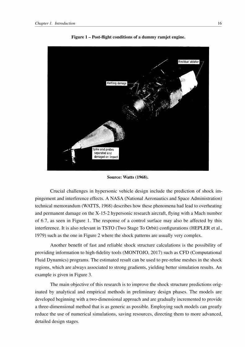
Figure 1 – Post-flight conditions of a dummy ramjet engine.
Source: Watts (1968).
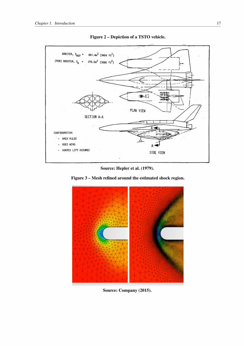
Crucial challenges in hypersonic vehicle design include the prediction of shock im-pingement and interference effects. A NASA (National Aeronautics and Space Administration)technical memorandum (WATTS, 1968) describes how these phenomena had lead to overheatingand permanent damage on the X-15-2 hypersonic research aircraft, flying with a Mach numberof 6.7, as seen in Figure 1. The response of a control surface may also be affected by thisinterference. It is also relevant in TSTO (Two Stage To Orbit) configurations (HEPLER et al.,1979) such as the one in Figure 2 where the shock patterns are usually very complex.
Another benefit of fast and reliable shock structure calculations is the possibility ofproviding information to high-fidelity tools (MONTOJO, 2017) such as CFD (ComputationalFluid Dynamics) programs. The estimated result can be used to pre-refine meshes in the shockregions, which are always associated to strong gradients, yielding better simulation results. Anexample is given in Figure 3.
The main objective of this research is to improve the shock structure predictions orig-inated by analytical and empirical methods in preliminary design phases. The models aredeveloped beginning with a two-dimensional approach and are gradually incremented to providea three-dimensional method that is as generic as possible. Employing such models can greatlyreduce the use of numerical simulations, saving resources, directing them to more advanced,detailed design stages.
Chapter 1. Introduction 17
Figure 2 – Depiction of a TSTO vehicle.
Source: Hepler et al. (1979).
Figure 3 – Mesh refined around the estimated shock region.
Source: Company (2015).

Chapter 1. Introduction 18
1.3 Thesis Structure
• Chapter 2: a brief bibliographic review of all compressible flow concepts and their relevanttechniques is presented.
• Chapter 3: presentation and development of the two-dimensional shock estimation method-ology, discussing its results and limitations.
• Chapter 4: presentation and development of the three-dimensional shock estimationmethodology, discussing its results and limitations, from mathematical, physical andcomputational standpoints.
• Chapter 5: potential models and avenues for future work are presented with final thoughtsand perspectives.

19
2 BIBLIOGRAPHIC REVIEW
The concepts and notations presented in this chapter follow those used in Anderson’sbooks (ANDERSON, 2002; ANDERSON, 2006) due to their widespread use.
2.1 Flow regimes
The local Mach number is a dimensionless flow parameter that governs many propertiesof a gas. It is defined as:
M =V/a (2.1)
where V is the local velocity and a the local speed of sound. Similarly, when referring to thenon-perturbed flow upstream of the body, the freestream Mach number definition is used:
M∞ =V∞/a∞ (2.2)
These numbers are also used to distinguish between flow regimes. Although they sharethe same general equations, their characteristics are significantly different and the solutionmethods drastically change along with the underlying assumptions. The nature of each flowregime is illustrated over the following subsections. Viscous effects, apart from the effect of ashock itself, are taken as negligible over the course of this study.
2.1.1 Subsonic flow
Flows in which the freestream velocity is below the speed of sound given by its propertiesare called subsonic flows. This translates mathematically as M < 1 everywhere in the flow field.Disturbances introduced on the flow, such as the presence of a body, propagate exactly likea conventional acoustic wave. The speed of sound is in fact the speed where such pressurefluctuations propagate throughout the flow field.
At subsonic speeds, these mechanical waves are able to reach upstream positions, mean-ing that fluid particles are displaced without being directly touched by the source of thesedisturbances. This ‘forewarning’ effect is a very important characteristic of the subsonic regime.Such speeds are typical of light propeller-driven aircraft, where M∞ < 0.8 in most cases.
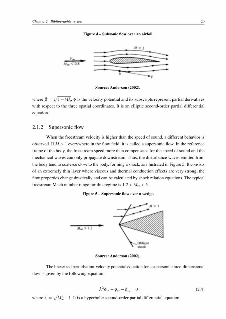
Subsonic flows such as the one shown in Figure 4 will not be treated directly in thepresent work. However, it is worth noting their qualitative behavior. For instance, the linearizedperturbation-velocity potential equation for a subsonic three-dimensional flow is of the form:
β2φxx +φyy +φzz = 0 (2.3)
Chapter 2. Bibliographic review 20
Figure 4 – Subsonic flow over an airfoil.
Source: Anderson (2002).
where β =√
1−M2∞, φ is the velocity potential and its subscripts represent partial derivatives
with respect to the three spatial coordinates. It is an elliptic second-order partial differentialequation.
2.1.2 Supersonic flow
When the freestream velocity is higher than the speed of sound, a different behavior isobserved. If M > 1 everywhere in the flow field, it is called a supersonic flow. In the referenceframe of the body, the freestream speed more than compensates for the speed of sound and themechanical waves can only propagate downstream. Thus, the disturbance waves emitted fromthe body tend to coalesce close to the body, forming a shock, as illustrated in Figure 5. It consistsof an extremely thin layer where viscous and thermal conduction effects are very strong, theflow properties change drastically and can be calculated by shock relation equations. The typicalfreestream Mach number range for this regime is 1.2 < M∞ < 5.
Figure 5 – Supersonic flow over a wedge.
Source: Anderson (2002).
The linearized perturbation-velocity potential equation for a supersonic three-dimensionalflow is given by the following equation:
λ2φxx−φyy−φzz = 0 (2.4)
where λ =√
M2∞−1. It is a hyperbolic second-order partial differential equation.
Chapter 2. Bibliographic review 21
2.1.3 Transonic flow
In the typical range of freestream Mach numbers between 0.8 < M∞ < 1.2 parts of theflow may be accelerated or decelerated, creating a mixed flow regime where both subsonic andsupersonic flow conditions are present. In terms of local Mach numbers, there are regions of theflow where M < 1 and others where M ≥ 1. The different natures of subsonic and supersonicflows make it a difficult fluid dynamics problem.
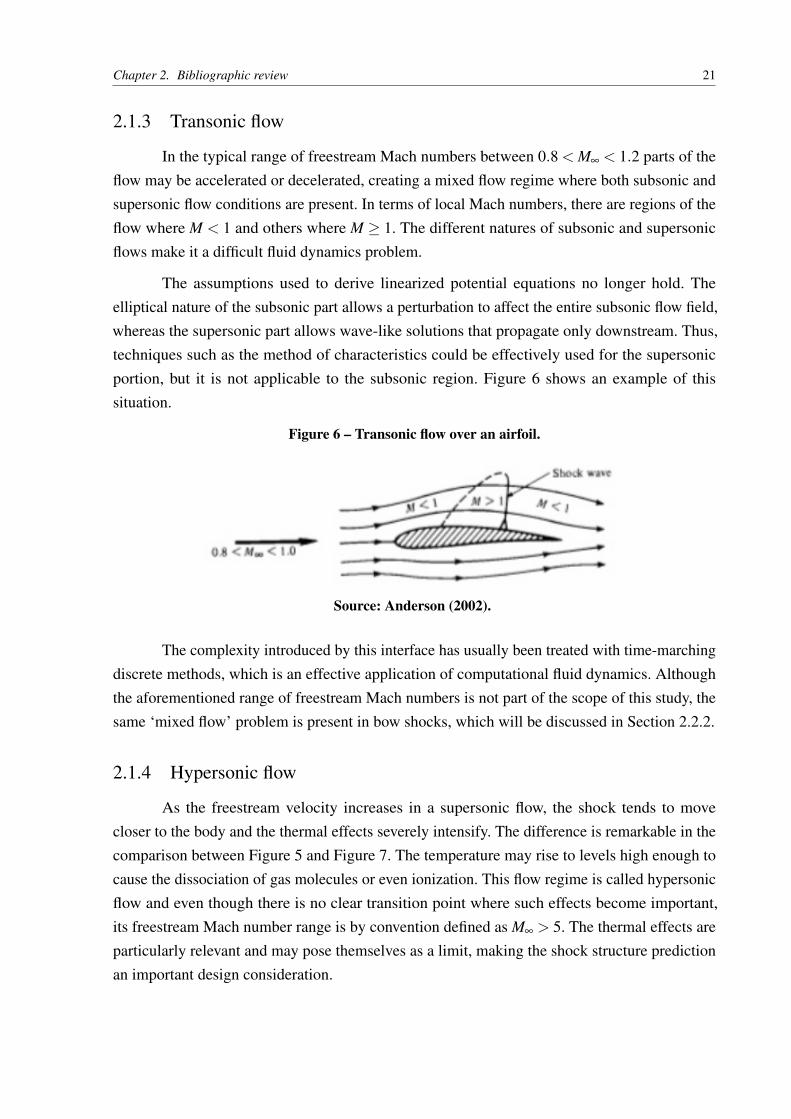
The assumptions used to derive linearized potential equations no longer hold. Theelliptical nature of the subsonic part allows a perturbation to affect the entire subsonic flow field,whereas the supersonic part allows wave-like solutions that propagate only downstream. Thus,techniques such as the method of characteristics could be effectively used for the supersonicportion, but it is not applicable to the subsonic region. Figure 6 shows an example of thissituation.
Figure 6 – Transonic flow over an airfoil.
Source: Anderson (2002).
The complexity introduced by this interface has usually been treated with time-marchingdiscrete methods, which is an effective application of computational fluid dynamics. Althoughthe aforementioned range of freestream Mach numbers is not part of the scope of this study, thesame ‘mixed flow’ problem is present in bow shocks, which will be discussed in Section 2.2.2.
2.1.4 Hypersonic flow
As the freestream velocity increases in a supersonic flow, the shock tends to movecloser to the body and the thermal effects severely intensify. The difference is remarkable in thecomparison between Figure 5 and Figure 7. The temperature may rise to levels high enough tocause the dissociation of gas molecules or even ionization. This flow regime is called hypersonicflow and even though there is no clear transition point where such effects become important,its freestream Mach number range is by convention defined as M∞ > 5. The thermal effects areparticularly relevant and may pose themselves as a limit, making the shock structure predictionan important design consideration.

Chapter 2. Bibliographic review 22
Figure 7 – Hypersonic flow over a wedge.
Source: Anderson (2002).
2.2 Shock formation
2.2.1 Attached shocks
When a supersonic flow meets an obstacle that tends to make it ‘turn on itself’ (ANDER-SON, 2002) such as a compression corner, an oblique shock wave is formed by the coalescenceof the disturbance waves produced by the ramp in a triangular or conical fashion, for two-dimensional and three-dimensional cases, respectively. If the flow deflection angle is sufficientlylow, an attached shock is formed. Figure 8 provides both schematic and real examples of thisphenomenon.
Figure 8 – Attached shock examples.
(a) Schematic of attached shock wave. (b) Shock wave attached to X15 at Mach number 3.5.
Source: Ziniu et al. (2013).
The equation that relates upstream the Mach number M1, the flow deviation angle θ andthe shock angle β is given by:
tanθ = 2cotβ
[M2
1 sin2β −1
M21(γ + cos2β )+2
](2.5)
Chapter 2. Bibliographic review 23
where γ is the specific heat ratio. This equation is also called the θ -β -M relation, as θ is givenexplicitly by the other two variables. However, the shock angle is often the unknown variableand this in turn forces the use of a numerical solver or a graphic-based solution. An alternativeform of this expression was derived by Emanuel (ANDERSON, 2002), expressing analyticallythe same relation as a cubic in tanβ , obtaining the following expression:
tanβ =M2
1 −1+2λ cos[(4πδ + cos−1 χ)/3]
3(
1+γ−1
2M2
1
)tanθ
(2.6)
where δ = 0 corresponds to the strong shock solution and δ = 1 gives the weak shock solution.The variables λ and χ are intermediate equations used to simplify the final expression, and aredefined by:
λ =
[(M2
1 −1)2−3(
1+γ−1
2M2
1
)(1+
γ +12
M21
)tan2
θ
]1/2
, (2.7)
χ =
(M21 −1)3−9
(1+
γ−12
M21
)(1+
γ−12
M21 +
γ +14
M41
)tan2 θ
λ 3 . (2.8)
These equations are also called the β -θ -M relation, as β is now the independent variable.No extra assumptions are used when this relation is derived, so it remains exact. The clearadvantage of these formulas is that numerical solvers are no longer needed, which often increasesprecision and reduces computational costs.
2.2.2 Detached shocks
The oblique shock relations can be solved graphically, yielding Figure 9. In the chart,every Mach number yields a different maximum flow deflection angle θmax that increasesasymptotically as M → ∞. For a given M, no oblique shock angle can be obtained beyondits respective θmax. In reality, a different phenomenon is observed, namely a detached shock,exemplified by Figure 10.
Detached shocks are formed in such a way that it stands at a distance upstream of thebody, often called stand-off distance. Moreover, the shock is curved and consequently the after-shock gas properties are not homogeneous. This is responsible for the appearance of propertygradients, the entropy gradient being one of those. Crocco’s gas dynamic equation for a steadyflow (ANDERSON, 2002) can be written as:
V× (∇×V) = ∇h0−T ∇s (2.9)

Chapter 2. Bibliographic review 24
Figure 9 – Oblique shock angle relation chart.
Source: NACA (1953).
Figure 10 – Detached shock examples.
(a) Schematic of detached shock wave. (b) Detached bow shock wave around Mer-cury Spacecraft.
Source: Ziniu et al. (2013).
where V is the velocity vector field, ∇h0 is the total enthalpy gradient and T ∇s is the entropygradient multiplied by the local temperature. The curl operator of the velocity vector field is alsodefined as the vorticity of a flow. Given that different shock angles produce different entropy
Chapter 2. Bibliographic review 25
changes for the same freestream conditions and that the total enthalpy does not change across ashock, there can only be an entropy gradient, meaning that the right hand side of the equation isnon-zero. Thus, in order to satisfy the expression, ∇×V 6= 0, the vorticity must also be non-zero.
This result implies that the flow behind a curved shock is rotational, rendering potential-based methods invalid. Furthermore, the non-oblique portion of the shock generates a subsonicpocket immediately behind it, surrounded by a supersonic part. As mentioned in Section 2.1.3,this makes it a complex problem, usually solved by time-marching computational techniques orempirical expressions (ANDERSON, 2002; ANDERSON, 2006).
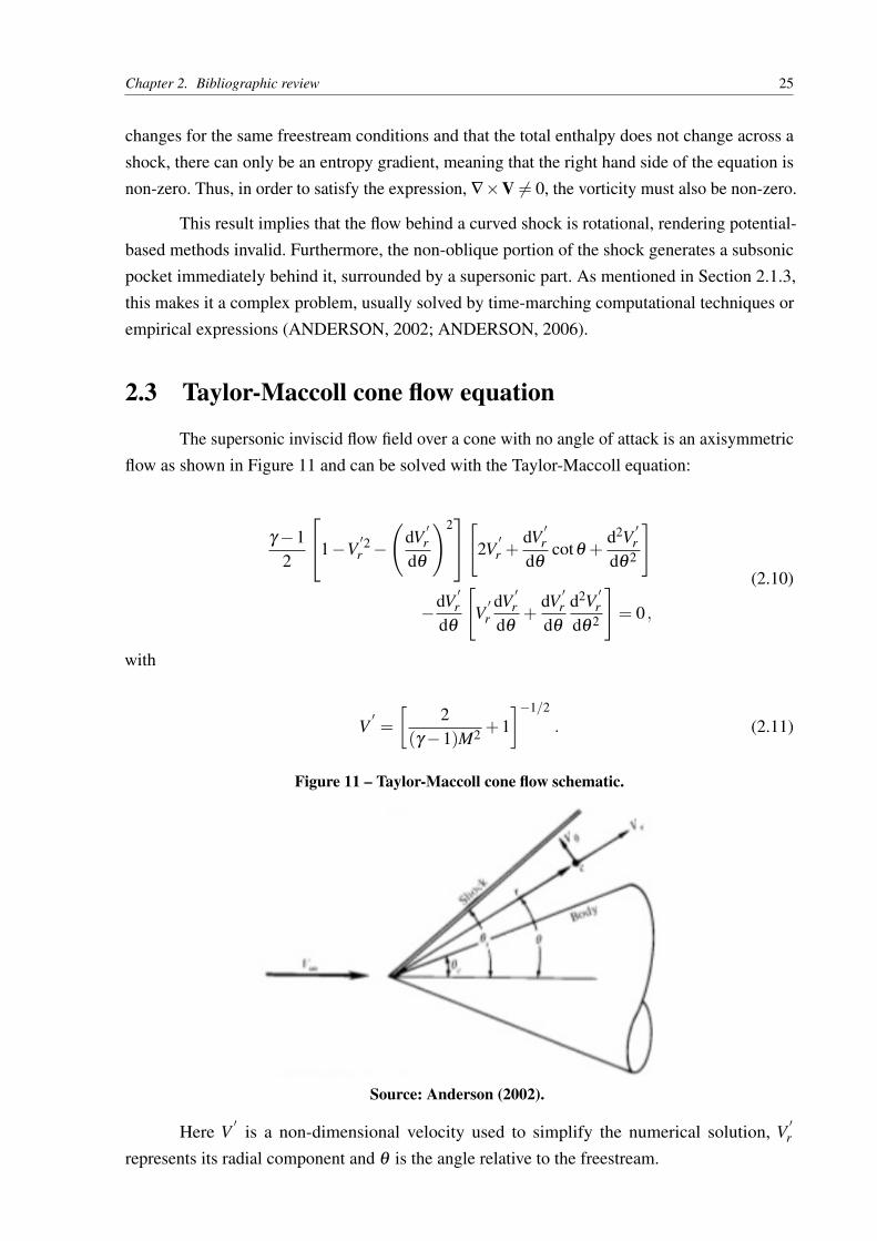
2.3 Taylor-Maccoll cone flow equation
The supersonic inviscid flow field over a cone with no angle of attack is an axisymmetricflow as shown in Figure 11 and can be solved with the Taylor-Maccoll equation:
γ−12
1−V′2r −
(dV
′r
dθ
)2[2V
′r +
dV′r
dθcotθ +
d2V′r
dθ 2
]
−dV′r
dθ
[V′r
dV′r
dθ+
dV′r
dθ
d2V′r
dθ 2
]= 0 ,
(2.10)
with
V′=
[2
(γ−1)M2 +1]−1/2
. (2.11)
Figure 11 – Taylor-Maccoll cone flow schematic.
Source: Anderson (2002).
Here V′
is a non-dimensional velocity used to simplify the numerical solution, V′r
represents its radial component and θ is the angle relative to the freestream.

Chapter 2. Bibliographic review 26
The flow past a cone can be solved numerically by the following algorithm:
• An initial shock angle is guessed.
• After-shock velocity components (Vr and Vθ ) are obtained through oblique shock relations.
• Equation 2.10 is solved with a numerical integration method.
• Imposing the flow tangency condition Vθ = 0, the shock angle is adjusted and the processis repeated until this condition is satisfied within a defined tolerance.
2.4 Local surface inclination methods
2.4.1 Tangent-Wedge and Tangent-Cone
In educational contexts, some simple pressure prediction methods are used and are mostlybased on the local surface inclination and knowledge of the freestream Mach number. One ofthem is the Tangent-Wedge method, used for two-dimensional sharp bodies. It is shown in Figure12 and it assumes that all body slopes are smaller than the maximum flow deflection angle(ANDERSON, 2006). The procedure is as follows:
• A tangent line is drawn from the surface point where the pressure should be calculated,crossing the symmetry axis.
• The angle obtained is used as the flow deflection angle of an equivalent wedge, hence thename. It is then used in the oblique shock equation, obtaining the shock angle.
• From oblique shock relations, the pressure can be calculated.
• Repeating this procedure all over the body with the desired resolution, the surface pressurescan be estimated.
The Tangent-Cone method is a natural axisymmetrical extension of the Tangent-Wedgemethod (ANDERSON, 2006). In a 3D flow, a tangent cone angle can be obtained and used inthe Taylor-Maccoll equation. As seen in Figure 13, the general procedure does not change.
2.4.2 Shock-Expansion method
Also employed exclusively in attached shock cases, a procedure often used to calculatelocal pressures is the Shock-Expansion method shown in Figure 14. Unlike the previous localsurface inclination methods, it has more solid theoretical foundations (ANDERSON, 2006). Thealgorithm is outlined as follows:

Chapter 2. Bibliographic review 27
Figure 12 – Illustration of the Tangent-Wedge method.
Source: Anderson (2006).
Figure 13 – Illustration of the Tangent-Cone method.
Source: Anderson (2006).
• Taking the tangent slope angle θn of the very first segment of the body, its oblique shockangle is calculated. From oblique shock relations, the after-shock Mach number is obtained.
• The flow along the surface streamline is assumed to be undergoing a Prandtl-Meyerexpansion over its course. Defining ∆θ = θn−θi, where θi is the body slope angle at thepoint of interest, the following expression holds:

Chapter 2. Bibliographic review 28
∆θ =
√γ +1γ−1
tan−1
√γ−1γ +1
(M2n −1)− tan−1
√γ−1γ +1
(M2i −1)
−[
tan−1√
M2n −1− tan−1
√M2
i −1].
(2.12)
• The local Mach number is then calculated numerically or graphically and all desiredproperties can be obtained through isentropic relations.
Figure 14 – Shock-Expansion method.
Source: Anderson (2006).
It is equally applicable for two-dimensional and axisymmetrical bodies (ANDERSON,2006). This model is close to being exact under the assumptions of inviscid flow, however,it ignores the effects of the multiple reflections of the expansion waves. Figure 15 illustratesqualitatively that as the Mach number increases and enters the Hypersonic flow, the Mach linestend to align more with the freestream, reducing these interactions. Therefore, the proceduretends to be more accurate in this regime. (ANDERSON, 2006)
Figure 15 – Reflection of expansion waves in different regimes.
(a) Reflection at supersonic speeds. (b) Reflection at hypersonic speeds.
Source: Anderson (2006).

29
3 2D SHOCK METHOD
3.1 Geometry generation
The method used for the two-dimensional shock calculation is the one proposed by thethesis of Herrera (MONTOJO, 2017). In this method, a 2D body is defined by a ‘polyline’, i.e. adiscretization in straight lines that shape an object. These are used as the input for the 2D shockmethod script, which is written with Python 3 as the programming language. This choice wasbased on its accessibility, versatility and its interface with C++ (FOUNDATION, 2012).
The coordinates are read from a .txt file, as pairs of x and y coordinates. For testingpurposes, a simple 2D body generation script was implemented. It consists in the evaluation ofa function that describes the body in multiple points and writing a coordinate .txt file with thedesired parameters and plotting the output body. It was used to generate many classical shapes,such as wedges, cylinders, blunt wedges, ellipses, sine waves, Von Karman ogives, etc.
All bodies are generated assuming symmetry conditions, implying that the stagnationpoint of the flow is always assumed to be at the most upstream location of the body. Angles ofattack are not treated at this stage.
3.2 Core principle of operation
3.2.1 Attached shock calculation
The core of the calculation is based on the tangent wedge method. Taking the mostupstream element of the 2D body, the first point of the shock structure is assumed to be onthe body’s tip. Since the body is discretized by points, the slope can be calculated from trivialanalytic geometry. This slope is used as the flow deflection angle, which is used along with thefreestream Mach number as inputs in the oblique shock equation, yielding the first oblique shockangle. Up to this point, this procedure is identical to the tangent wedge method, discussed inSection 2.4.1.
Figure 16 – Step by step depiction of the attached shock method.
Source: Montojo (2017).
However, the expansion of the flow has to be taken into account. Therefore, an alternativeis proposed. The five steps illustrated in Figure 16 can be broken down as follows:

Chapter 3. 2D Shock Method 30
• The method begins exactly as in the tangent wedge, with the current body line segmentrepresented as a black line, and the shock line segment as the red line. The 2D body as awhole is shown in gray line segments.
• The shock line segment is then limited by its intersection with a Mach wave emitted atthe end of the respective body line segment, shown as a dashed blue line. This Machwave is generated with the local after-shock Mach number, with an angle given by µ =
arcsin(1/M).
• The next shock line segment is calculated using the previous shock line segment (in green)as the starting point and the current body slope is used in the oblique shock equation.
• The shock line segment is once again limited by its respective Mach line.
• This process is continued successively up to the end of the body.
This procedure is actually a simplification of the shock-expansion method and calculationerrors are propagated forward since each result strictly depends on the previous one. Figure 17shows a trivial case of a 12.17◦ wedge in two flows with different freestream velocities, M∞ = 4and M∞ = 15. The resulting shock angles are 24.27◦ and 15.66◦ respectively as expected. As theMach number increases and enters the hypersonic regime, the shock moves closer to the body.The Mach lines are mainly traced for demonstration and debugging purposes.
Other examples will be shown and compared to numerical simulations in Section 3.4.
3.2.2 Detached shock calculation
As discussed in Sections 2.1.3 and 2.2.2, a detached shock cannot be treated in the sameway as an attached one. Evidently, there is no oblique shock solution in this case so the previousprocedure cannot be used as a starting point. A different strategy must be adopted. In the presentwork, an empiric approach was used, called Billig’s hyperbola (BILLIG, 1967).
The solution provided by Billig describes bow shocks on cylindrical or spherical-nosedbodies as hyperbolas, for a given curvature radius and Mach number. The proposed formulae fora cylindrical-nosed body are Eq. 3.1 to 3.3.
x = R+∆−Rc cot2 µ
[(1+
y2 tan2 µ
R2c
)1/2
−1
], (3.1)
∆/R = 0.386exp(4.67/M2
∞
), (3.2)
Rc/R = 1.386exp[1.8/(M∞−1)0.75
]. (3.3)

Chapter 3. 2D Shock Method 31
Figure 17 – Simple wedge shock examples. The orange line is the body, the blue line is the shockand the dashed lines are Mach lines.
(a) 2D attached shock method applied to a 12.17◦ wedge at M∞ = 4.
(b) 2D attached shock method applied to a 12.17◦ wedge at M∞ = 15.
Source: The author (2018).
where x and y are geometric coordinates, R is the body nose’s radius of curvature, ∆ is the shockstand-off distance, Rc is the hyperbola’s radius of curvature, µ is the freestream Mach angle such
Chapter 3. 2D Shock Method 32
that µ = arcsin(1/M∞).
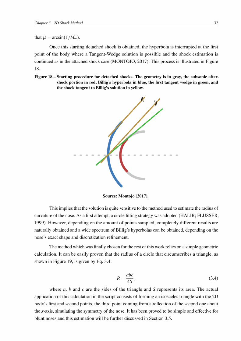
Once this starting detached shock is obtained, the hyperbola is interrupted at the firstpoint of the body where a Tangent-Wedge solution is possible and the shock estimation iscontinued as in the attached shock case (MONTOJO, 2017). This process is illustrated in Figure18.
Figure 18 – Starting procedure for detached shocks. The geometry is in gray, the subsonic after-shock portion in red, Billig’s hyperbola in blue, the first tangent wedge in green, andthe shock tangent to Billig’s solution in yellow.
Source: Montojo (2017).
This implies that the solution is quite sensitive to the method used to estimate the radius ofcurvature of the nose. As a first attempt, a circle fitting strategy was adopted (HALIR; FLUSSER,1999). However, depending on the amount of points sampled, completely different results arenaturally obtained and a wide spectrum of Billig’s hyperbolas can be obtained, depending on thenose’s exact shape and discretization refinement.
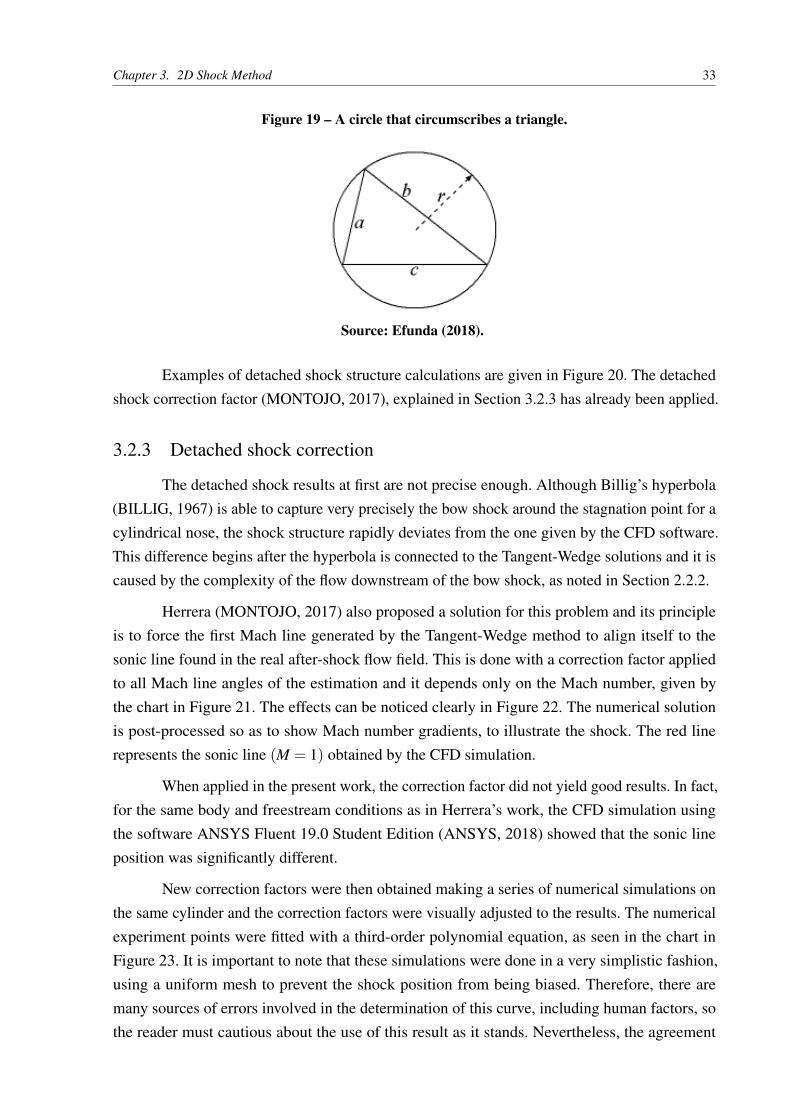
The method which was finally chosen for the rest of this work relies on a simple geometriccalculation. It can be easily proven that the radius of a circle that circumscribes a triangle, asshown in Figure 19, is given by Eq. 3.4:
R =abc4S
, (3.4)
where a, b and c are the sides of the triangle and S represents its area. The actualapplication of this calculation in the script consists of forming an isosceles triangle with the 2Dbody’s first and second points, the third point coming from a reflection of the second one aboutthe x-axis, simulating the symmetry of the nose. It has been proved to be simple and effective forblunt noses and this estimation will be further discussed in Section 3.5.
Chapter 3. 2D Shock Method 33
Figure 19 – A circle that circumscribes a triangle.
Source: Efunda (2018).
Examples of detached shock structure calculations are given in Figure 20. The detachedshock correction factor (MONTOJO, 2017), explained in Section 3.2.3 has already been applied.
3.2.3 Detached shock correction
The detached shock results at first are not precise enough. Although Billig’s hyperbola(BILLIG, 1967) is able to capture very precisely the bow shock around the stagnation point for acylindrical nose, the shock structure rapidly deviates from the one given by the CFD software.This difference begins after the hyperbola is connected to the Tangent-Wedge solutions and it iscaused by the complexity of the flow downstream of the bow shock, as noted in Section 2.2.2.
Herrera (MONTOJO, 2017) also proposed a solution for this problem and its principleis to force the first Mach line generated by the Tangent-Wedge method to align itself to thesonic line found in the real after-shock flow field. This is done with a correction factor appliedto all Mach line angles of the estimation and it depends only on the Mach number, given bythe chart in Figure 21. The effects can be noticed clearly in Figure 22. The numerical solutionis post-processed so as to show Mach number gradients, to illustrate the shock. The red linerepresents the sonic line (M = 1) obtained by the CFD simulation.
When applied in the present work, the correction factor did not yield good results. In fact,for the same body and freestream conditions as in Herrera’s work, the CFD simulation usingthe software ANSYS Fluent 19.0 Student Edition (ANSYS, 2018) showed that the sonic lineposition was significantly different.
New correction factors were then obtained making a series of numerical simulations onthe same cylinder and the correction factors were visually adjusted to the results. The numericalexperiment points were fitted with a third-order polynomial equation, as seen in the chart inFigure 23. It is important to note that these simulations were done in a very simplistic fashion,using a uniform mesh to prevent the shock position from being biased. Therefore, there aremany sources of errors involved in the determination of this curve, including human factors, sothe reader must cautious about the use of this result as it stands. Nevertheless, the agreement

Chapter 3. 2D Shock Method 34
Figure 20 – Detached shocks over cylinders at different Mach numbers. The body is in blue, theshock in black and Mach lines in dashed red.
(a) 2D detached shock method applied to a cylinder at M∞ = 6.
(b) 2D detached shock method applied to a cylinder at M∞ = 8.
Source: The author (2018).
between the CFD solution and the shock structure prediction was greatly improved.

Chapter 3. 2D Shock Method 35
Figure 21 – Herrera’s correction factor chart. (MONTOJO, 2017)
Source: Montojo (2017).
3.2.4 Expansion segments and concavities
Oblique shock solutions are only possible for flow deflections that make the streamlinesturn into themselves, which correspond to positive flow deflection angles in the reference frameof Figure 9. However, for robustness purposes, the script is required to be capable of dealingwith negative angles, such as the ones found on a diamond wedge.
In practice, it represents an isentropic expansion. Although expansions do interact withthe general shock structure, their interaction is rather complex and its effects for the purposesof this low-fidelity approximation are considered negligible (MONTOJO, 2017; ANDERSON,2002). Hence, the algorithm must safely identify negative angle line segments and ignore theirpresence.
A convex body, in this case a polygon, is by definition one in which all line segmentsbetween two points on the boundary remain inside the domain. Whenever there is a line segmentthat has a more positive slope angle than the previous one, a concavity appears. Concave sectionsmay generate other shocks. Hence, concavities must be properly identified and dealt with.
A concavity starts at the point that precedes the increase in flow deflection angle and endswhere it decreases once again. Mach lines from both extremities are traced and their intersection
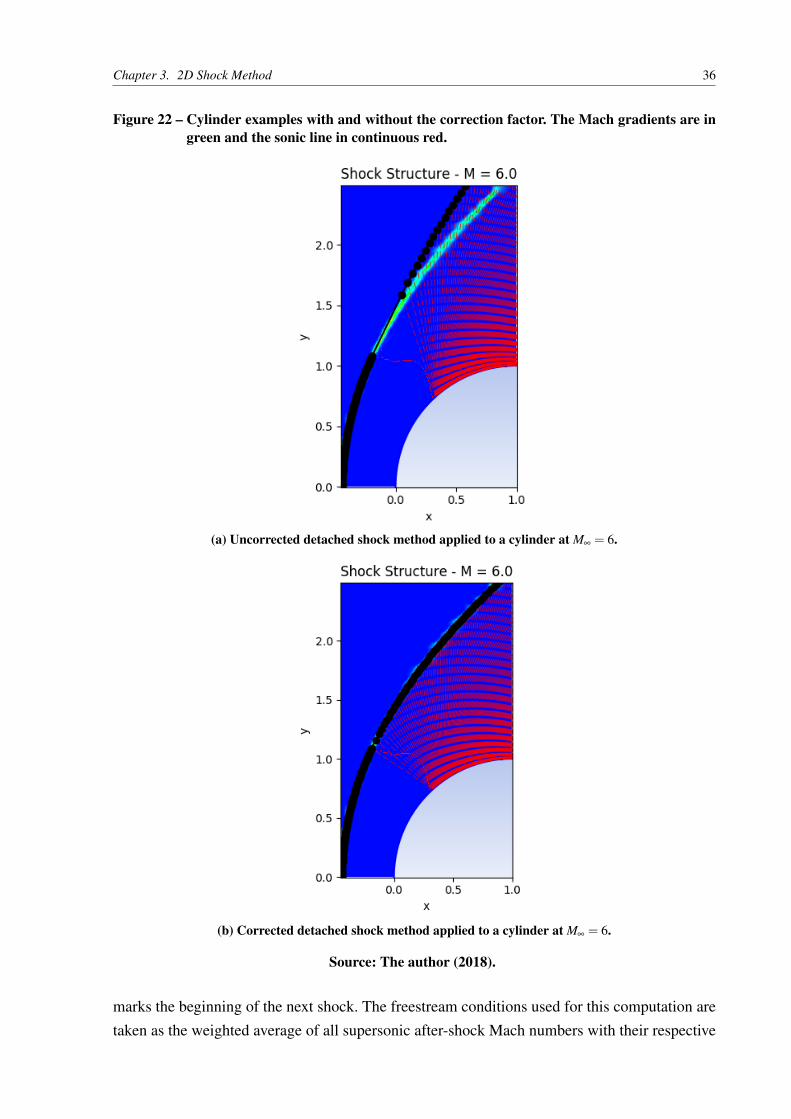
Chapter 3. 2D Shock Method 36
Figure 22 – Cylinder examples with and without the correction factor. The Mach gradients are ingreen and the sonic line in continuous red.
(a) Uncorrected detached shock method applied to a cylinder at M∞ = 6.
(b) Corrected detached shock method applied to a cylinder at M∞ = 6.
Source: The author (2018).
marks the beginning of the next shock. The freestream conditions used for this computation aretaken as the weighted average of all supersonic after-shock Mach numbers with their respective

Chapter 3. 2D Shock Method 37
Figure 23 – New correction factor chart.
Source: The author (2018).
length, discarding all subsonic after-shock values. With the first point defined, the shock structureestimation is carried on as described in Section 3.2.1. A simple example can be seen in Figure24.
Figure 24 – Multiple shock example on a wedge with three slopes.
Source: The author (2018).

Chapter 3. 2D Shock Method 38
3.3 Body segmentation
After the raw 2D coordinate data is imported into the shock structure calculation script,its different parts must be identified. This was done under an object-oriented programming (OOP)concept. In this context, each part is called a segment and should not be confused with a linesegment. Here, a segment is the ensemble of line segments and points with an specific behaviorwith respect to the calculation.
The main advantage of the body segmentation is an effective modularization of parts thathave different interactions with the shock structure and separate storage of their information. Theprocedure goes as follows:
• As a first step, all body slopes are calculated and stored.
• The first slope angle is checked for its sign. If positive, it marks the beginning of a convexsegment. If zero or negative, it is an expansion segment. The first segment is never aconcave one.
• The script continues adding points and slopes to the current segment and the slope anglesare tested in each iteration.
• In the convex case, when a negative slope angle is encountered, the current segment isstored and an expansion segment begins. If the next slope angle is actually larger than theprevious one, above a tolerance defined to prevent noise and machine imprecision generatedconcavities, a concave segment begins. Otherwise, the convex segment continues.
• In the expansion case, if a positive slope angle is encountered, the current segment is storedand a concave segment begins. Otherwise, the expansion segment continues. It cannotinitiate directly a convex segment.
• In the concave case, if a zero or negative slope angle is encountered, the current segmentis stored and an expansion segment begins. If the next slope angle is smaller than theprevious one, a convex segment begins. Otherwise, the concave segment continues.
Some segmentation examples are shown in Figure 25.
3.4 2D results and analysis
The examples shown in this section are compared to CFD simulations performed withAnsys Fluent 19.0 - Student Edition (ANSYS, 2018), using inviscid, ideal gas models withdensity based solvers in a two-dimensional flow and a uniform mesh.
Chapter 3. 2D Shock Method 39
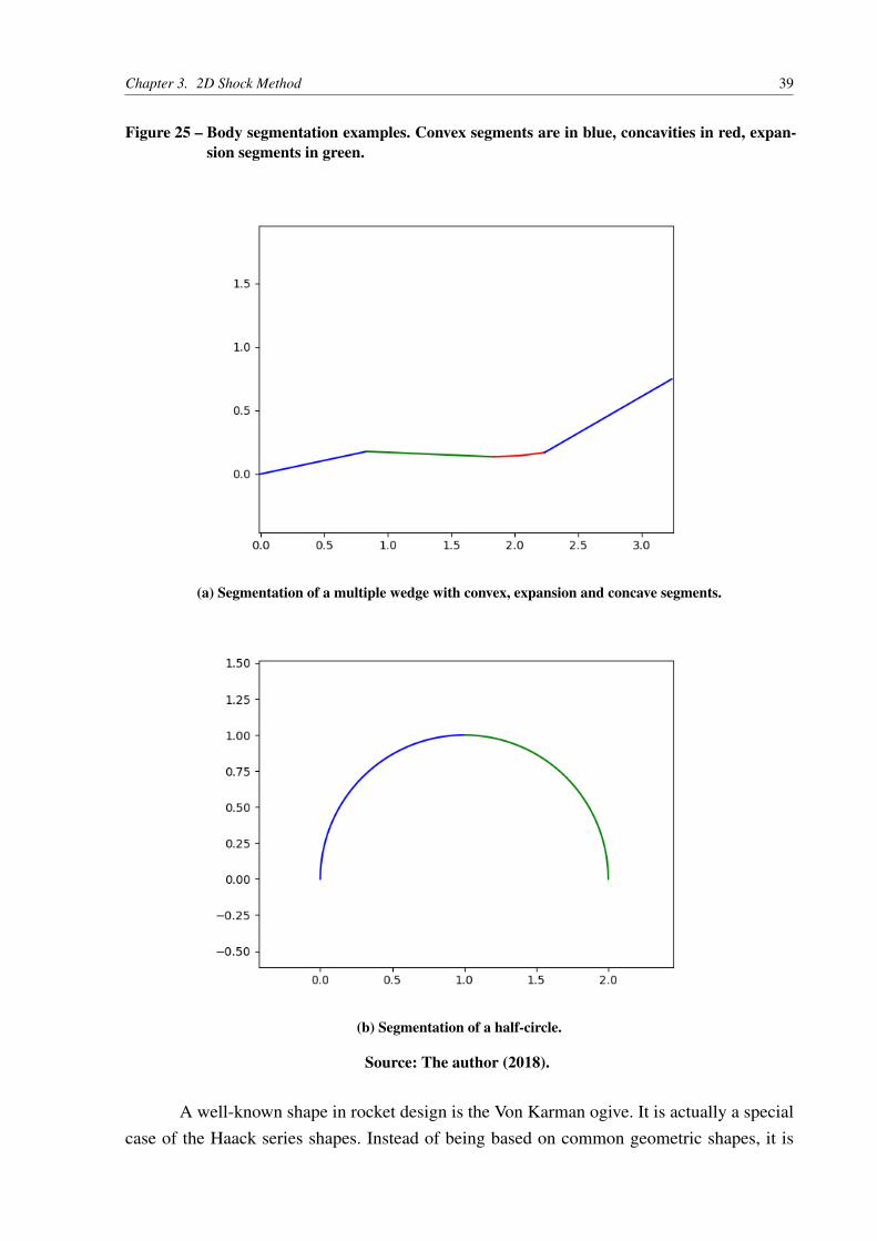
Figure 25 – Body segmentation examples. Convex segments are in blue, concavities in red, expan-sion segments in green.
(a) Segmentation of a multiple wedge with convex, expansion and concave segments.
(b) Segmentation of a half-circle.
Source: The author (2018).
A well-known shape in rocket design is the Von Karman ogive. It is actually a specialcase of the Haack series shapes. Instead of being based on common geometric shapes, it is

Chapter 3. 2D Shock Method 40
derived from a mathematical expression, optimized to reduce drag. The Haack series is given by:
θ = arccos(
1− 2xL
), (3.5)
y =R√π
√θ − sin(2θ)
2+C sin3
θ , (3.6)
where θ is a geometric parameter, L is the total length of the ogive, R is the maximum ogiveradius and C is the Haack series parameter. The latter has a strong influence over the generalshape of the curve and the drag coefficient. For a given length and radius, the curve that minimizesthe drag is obtained by setting C = 0, which is precisely the Von Karman ogive (DING et al.,2015).
The Haack series does not yield very sharp nose tips, disallowing attached shock solutions.For testing purposes, the Von Karman ogive equation was multiplied by 0.5 on the y variable,generating a sharper ogive. The results are seen in Figure 26. Once again, Mach number gradientsare used in the post-processing. The agreement between the solutions is satisfactory. Theuncompressed Von Karman ogive simulation is shown in Section 3.5.2.
Another example of a standard polyline is a blunted wedge, as shown in Figure 27. Theexpressions of the polyline are given by circle and line equations, united at the tangency point:
xt =L2
R
√r2
nR2 +L2 , (3.7)
yt =xtRL
, (3.8)
where (xt ,yt) is the tangency point and rn is the nose cap radius. The simulation example is givenin Figure 28. The agreement between the solutions is also deemed satisfactory.
3.5 2D model limitations
3.5.1 Large slope discontinuity
Over the course of the development of the 2D shock structure prediction algorithm,several limitations were found. Although some of them were found in fairly extreme cases, it isessential to determine the weaknesses of the method, even in a low-fidelity modeling phase. Sucherrors, when not monitored appropriately, may lead to undesired and even unpredictable behaviorin a Multidisciplinary Design Optimization (MDO), forcing the appearance of ill-calculated oreven physically impossible solutions.
For instance, a sudden large decrease of the flow deflection angle causes a significantisentropic expansion. The shock prediction script overestimates its influence and the shock
Chapter 3. 2D Shock Method 41
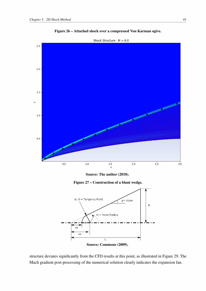
Figure 26 – Attached shock over a compressed Von Karman ogive.
Source: The author (2018).
Figure 27 – Construction of a blunt wedge.
Source: Commons (2009).
structure deviates significantly from the CFD results at this point, as illustrated in Figure 29. TheMach gradient post-processing of the numerical solution clearly indicates the expansion fan.
Chapter 3. 2D Shock Method 42
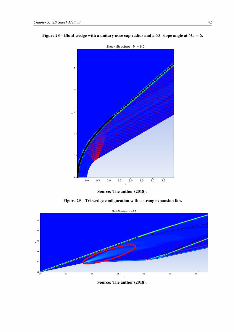
Figure 28 – Blunt wedge with a unitary nose cap radius and a 60◦ slope angle at M∞ = 6.
Source: The author (2018).
Figure 29 – Tri-wedge configuration with a strong expansion fan.
Source: The author (2018).

Chapter 3. 2D Shock Method 43
3.5.2 After-shock Mach number gradients
Multi-shock situations, observed in the presence of concavities, are also quite complex tomodel. This is due to the fact that as the after-shock flow expands over the body, the local Machnumbers change differently over the body, creating a Mach number gradient. This means that the‘freestream conditions’ seen by the subsequent shock are non-uniform.
For instance, the shock structure of an Von Karman ogive with its original equationas defined in Section 3.4 and followed by a wedge was calculated and numerically simulatedyielding Figure 30. Regardless of the choice of shock-expansion methods or after-shock Machaveraging, this error is still present and cannot be treated at this level of modeling fidelity.Although the fitting of the first shock seems very good, further corrections have been appliedand they are the subject of Section 3.5.3.
Figure 30 – A Von Karman ogive followed by a wedge illustrating multi-shock errors. The heatmap of the CFD represents local Mach numbers, going from red (highest) to blue (low-est).
Source: The author (2018).
3.5.3 Non-circular body noses
Although Billig’s hyperbola was specifically designed for cylinder and spheres, this isnot always the case in the context of optimizations and conceptual designs. Ideally, the algorithm
Chapter 3. 2D Shock Method 44
should be able to deal with that possibility without significant errors.
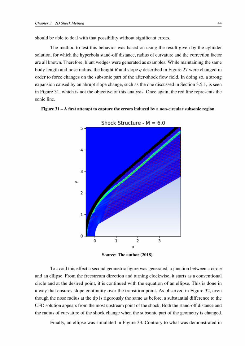
The method to test this behavior was based on using the result given by the cylindersolution, for which the hyperbola stand-off distance, radius of curvature and the correction factorare all known. Therefore, blunt wedges were generated as examples. While maintaining the samebody length and nose radius, the height R and slope q described in Figure 27 were changed inorder to force changes on the subsonic part of the after-shock flow field. In doing so, a strongexpansion caused by an abrupt slope change, such as the one discussed in Section 3.5.1, is seenin Figure 31, which is not the objective of this analysis. Once again, the red line represents thesonic line.
Figure 31 – A first attempt to capture the errors induced by a non-circular subsonic region.
Source: The author (2018).
To avoid this effect a second geometric figure was generated, a junction between a circleand an ellipse. From the freestream direction and turning clockwise, it starts as a conventionalcircle and at the desired point, it is continued with the equation of an ellipse. This is done ina way that ensures slope continuity over the transition point. As observed in Figure 32, eventhough the nose radius at the tip is rigorously the same as before, a substantial difference to theCFD solution appears from the most upstream point of the shock. Both the stand-off distance andthe radius of curvature of the shock change when the subsonic part of the geometry is changed.
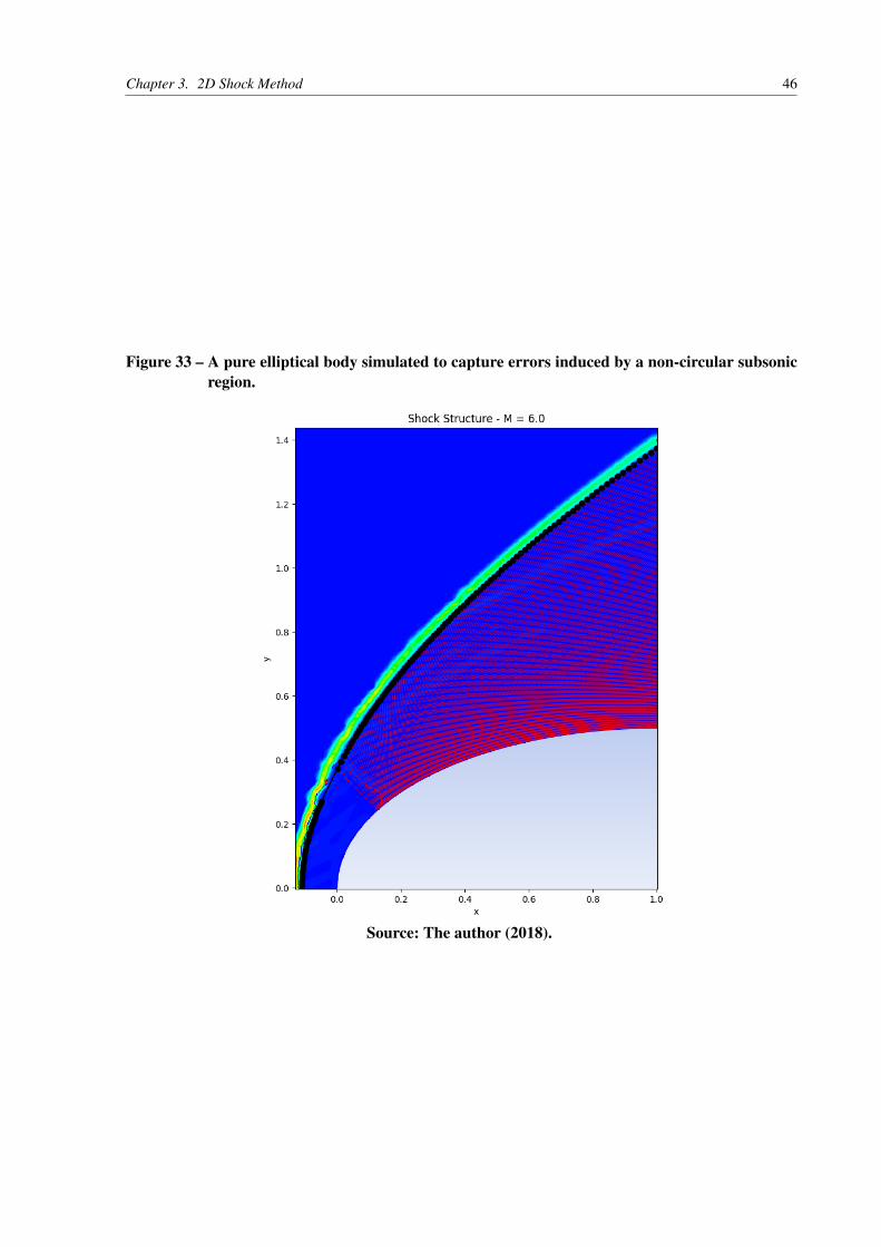
Finally, an ellipse was simulated in Figure 33. Contrary to what was demonstrated in

Chapter 3. 2D Shock Method 45
Figure 32 – Circle-ellipse body simulation before and after radius correction.
(a) Circle-ellipse body simulation withoutradius correction.
(b) Circle-ellipse body simulation with ra-dius correction.
Source: The author (2018).
Figure 32, the tendency in the pure ellipse case was to underestimate the stand-off distance.
The solution can be improved by changing the radius that is used as input to Billig’shyperbola equation to better fit the numerical results. This, at first, would require a case bycase study which is by no means useful in a preliminary design context. The author proposes,nevertheless, the study of a weighted average of the radii of curvature present in the subsonicsection of the shock. This could be based either on the angle of the radial line to the evaluatedpoint with respect to the freestream direction or the distance from the evaluated point to thestagnation point.
Such a model would require a great amount of numerical simulation with differentgeometries and Mach numbers. Therefore, despite its importance, it was considered out of scopefor the present work, but it is still noteworthy.
Chapter 3. 2D Shock Method 46
Figure 33 – A pure elliptical body simulated to capture errors induced by a non-circular subsonicregion.
Source: The author (2018).

47
4 3D SHOCK METHOD
The third dimension naturally adds a great amount of complexity. To deal with all thegeometric manipulations in a effective and fast way, the Computational Geometry AlgorithmsLibrary (CGAL) (The CGAL Project, 2018) was chosen. It was developed by a partnershipbetween several institutions. By default, this requires the use of the programming language C++,which also brings performance as a secondary but invaluable benefit.
Streamlines are curves along the surface of the body that are tangent to the velocity field,and in a steady flow, they effectively represent the flow deviation angles. In short, the goal of the3D shock prediction method is to efficiently cover the body with streamlines, to send this data tothe 2D shock method and to adapt its output to represent a 3D shock structure.
4.1 Geometry generation
Geometries in the two-dimensional case were always represented with piecewise-linearcurves, read from a simple text file containing pairs of coordinates. A three-dimensional body onthe other hand needs to be represented by a surface. The triangular Surface Mesh data structure(BOTSCH et al., 2018) from CGAL was chosen for this. It is based on the Half-Edge datastructure described in Figure 34.
Figure 34 – Half-Edge structure schematic.
Source: Botsch et al. (2018).
Each edge of the mesh is built as a pair of antiparallel oriented half-edges. Each half-edgestores a references to its incident vertex and to its incident face, except when it is on a border. Italso stores a reference to the next and previous half-edges that share the same incident face. Inaddition, each face and each vertex are associated to their incident half-edge.

Chapter 4. 3D Shock Method 48
Although Herrera proposed the use of CGAL’s Polyhedral Meshes, which is pointer-based, the Surface Mesh structure was preferred, which is index-based. The reason is thatthe algorithm can just as easily circulate around the mesh as it has the same underlying half-edge structure concept, with all the inter-element references stored in the structure, and themanipulation of indexes and property association is judged by the author as more straightforwardand intuitive.
As in the 2D geometry generation in Section 3.1, an algorithm was used to create 3Dmeshes. CGAL offers many tools to do so. In the axisymmetric case, the body can be thought ofas a surface of revolution of a 2D polyline around the symmetry axis. Simple techniques suchas creating polylines with regular azimuthal spacing between them and triangulation methodssuch as the Advancing Front Surface Reconstruction (DA; COHEN-STEINER, 2018) are able tocreate very regular, well-behaved meshes. Recalling the purpose of the algorithm, which is todevelop a robust tool, a different meshing method was used.
CGAL’s Implicit Surface generation uses an implicit user-defined function such that itsroots are taken as the points of the surface. To do so, a sphere is created at a desired center pointand points within the sphere query the implicit function in a randomized way. For the implicitfunction of an axisymmetric body, using x as the freestream direction coordinate in a Cartesian(x,y,z) system, every cross-section of the surface in the yz plane yields a circle:
f (x,y,z) = y2 + z2−R(x)2 , (4.1)
where R(x) is the function of the radius of the axisymmetric body. It is implemented by readinga polyline that outlines the body and using Barycentric Rational Interpolation from the Boostlibrary (PROJECT, 2018). Thus, the result is a fairly irregular surface. This is interesting from atesting and debugging standpoint, as a real surface input in an optimization algorithm is seldomvery regular. The mesh is output to an .off file (Object File Format), which is easily treated byCGAL. It is structured as a text file containing a first line with the total number of vertices, facesand edges, followed by a list of x,y,z coordinates and finally a list of faces composed by theindexes of its vertices, providing connectivity information.
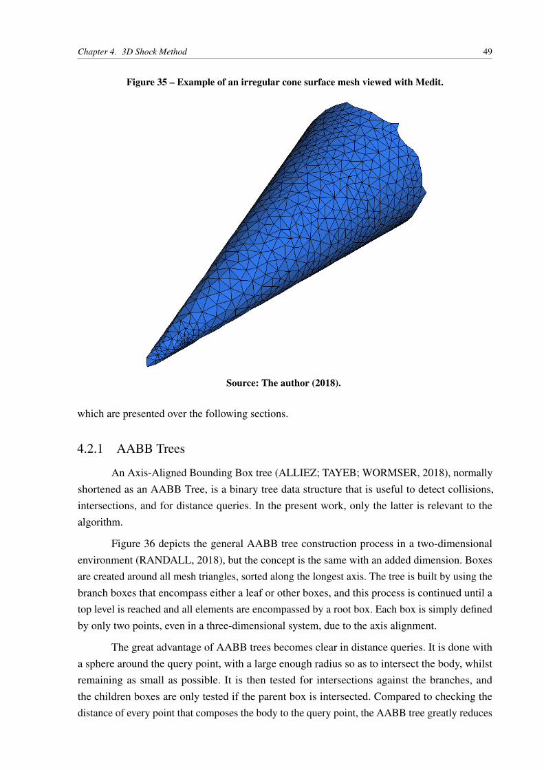
To visualize the mesh, the open-source software Medit (FREY, 2001), developed by theLaboratoire Jacques-Louis Lions (LJLL) was used. However, it uses .mesh extension files asinput, so the software Meshio (SCHLÖMER, 2018), which is also open-source, was employed toperform the .off to .mesh file conversion. Figure 35 demonstrates an example of a mesh generatedwith this procedure.
4.2 Solution setup
The 3D shock structure prediction algorithm begins by reading the input .off file andstoring it as a surface mesh structure. The algorithm then requires a series of tools and operations
Chapter 4. 3D Shock Method 49
Figure 35 – Example of an irregular cone surface mesh viewed with Medit.
Source: The author (2018).
which are presented over the following sections.
4.2.1 AABB Trees
An Axis-Aligned Bounding Box tree (ALLIEZ; TAYEB; WORMSER, 2018), normallyshortened as an AABB Tree, is a binary tree data structure that is useful to detect collisions,intersections, and for distance queries. In the present work, only the latter is relevant to thealgorithm.
Figure 36 depicts the general AABB tree construction process in a two-dimensionalenvironment (RANDALL, 2018), but the concept is the same with an added dimension. Boxesare created around all mesh triangles, sorted along the longest axis. The tree is built by using thebranch boxes that encompass either a leaf or other boxes, and this process is continued until atop level is reached and all elements are encompassed by a root box. Each box is simply definedby only two points, even in a three-dimensional system, due to the axis alignment.
The great advantage of AABB trees becomes clear in distance queries. It is done witha sphere around the query point, with a large enough radius so as to intersect the body, whilstremaining as small as possible. It is then tested for intersections against the branches, andthe children boxes are only tested if the parent box is intersected. Compared to checking thedistance of every point that composes the body to the query point, the AABB tree greatly reduces

Chapter 4. 3D Shock Method 50
Figure 36 – 2D AABB Tree construction algorithm.
Source: Botsch et al. (2018).
computational costs, especially when a large number of queries is necessary, outweighing theresources used to build the structure.
The AABB tree is used in the algorithm to project points over the surface as mentionedin Section 4.3. A generic example of an AABB Tree on a 3D body is provided in Figure 37.
Figure 37 – Generic 3D AABB Tree example.
Source: Alliez, Tayeb and Wormser (2018).
4.2.2 Surface velocity field
The streamlines are obtained with the aid of a surface velocity interpolation procedure.First, all vertex normal vectors are calculated. A vertex normal is defined as the normalizedaverage of all the normal vectors of the surfaces that contain the vertex, weighted by theirrespective area as in Figure 38. CGAL provides an automatic method to do so (LORIOT;TOURNOIS; YAZ, 2018). Furthermore, these normal vectors are easily stored and associated tothe surface mesh with CGAL’s property maps (BOTSCH et al., 2018).

Chapter 4. 3D Shock Method 51
Figure 38 – Vertex normals of a dodecahedral mesh.
Source: Commons (2012).
The freestream velocity vector is then project over each vertex, producing the surfacevelocity interpolant vector and stored once again in the property map:
Vv = V∞− (n ·V∞)n (4.2)
where Vv is the vertex velocity vector, n the vertex normal vector and V∞ the freestream velocityvector.
4.3 Streamline integration
The streamlines are integrated in reverse with respect to time, from downstream toupstream. This is done in order to ensure better coverage of the body.
A vector containing all facet centroid points is created as a reference (MONTOJO, 2017).Associated to each point, a boolean variable determines whether a point is already eliminatedfrom the calculation, as explained in Section 4.3.1. This centroid list is ordered in such a way sothat the most downstream points are placed first in the list in an attempt to generate the longeststreamlines.
The first available centroid point of the vector is taken as the first streamline and itslocal velocity is calculated as a barycentric average of the adjacent vertex velocity vectors. Inthe case of a centroid this is trivial as every vector has the same weight. In the general case, aplane is created with the three vertices and the query point is projected onto it. Using CGAL’s2D Barycentric Triangle Coordinates (ANISIMOV et al., 2018), the surface velocity vector iscalculated as:
Vs =W1Vv1 +W2Vv2 +W3Vv3 (4.3)

Chapter 4. 3D Shock Method 52
where Vs is the surface velocity vector and W is the barycentric averaging weight. The surfacevelocity and position are used as inputs for the streamline integration. A time step must then bedetermined. Herrera suggests the use of the quotient between the mean minimum triangle edgelength and the maximum surface velocity modulus which has been adopted in our script. Theequations to be integrated are simply the fluid kinematic equations:
dxdt
= Vs(x) , (4.4)
where x is the position, and t the time. Each component of the velocity vector is integrated sepa-rately forming an ordinary differential equation system. The integration method is implementedwith Boost library’s Odeint integrator (PROJECT, 2018), using a fourth-order Runge-Kuttamethod. After the integration step, the output is a point that is usually not directly on the surface.
This point is then used as a query point to the AABB tree, re-projecting the streamlinepoint over the surface. It is stored as a streamline point and the barycentric averaging process andits subsequent steps are repeated. This cycle continues up to a point where the change from theprevious streamline point to the next after its re-projection is within the user-specified tolerance.
Figure 39 – Streamlines traced over a cone.
Source: The author (2018).
Once this streamline is stored, the next one begins by searching the first non-eliminatedcentroid point on the centroid vector. Figure 39 shows an example of this intermediary result.
Chapter 4. 3D Shock Method 53
4.3.1 Stopping criterion and KD-Tree
When the streamlines are computed as explained in Section 4.3, a stopping criterion mustbe determined ensuring that the surface has been appropriately covered. The aforementionedcentroid list keeps track of what parts of the body have already been calculated.
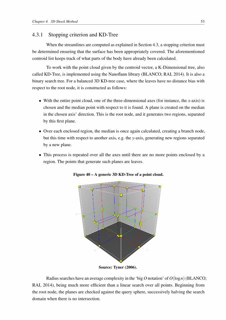
To work with the point cloud given by the centroid vector, a K-Dimensional tree, alsocalled KD-Tree, is implemented using the Nanoflann library (BLANCO; RAI, 2014). It is also abinary search tree. For a balanced 3D KD-tree case, where the leaves have no distance bias withrespect to the root node, it is constructed as follows:
• With the entire point cloud, one of the three-dimensional axes (for instance, the x-axis) ischosen and the median point with respect to it is found. A plane is created on the medianin the chosen axis’ direction. This is the root node, and it generates two regions, separatedby this first plane.
• Over each enclosed region, the median is once again calculated, creating a branch node,but this time with respect to another axis, e.g. the y-axis, generating new regions separatedby a new plane.
• This process is repeated over all the axes until there are no more points enclosed by aregion. The points that generate such planes are leaves.
Figure 40 – A generic 3D KD-Tree of a point cloud.
Source: Tyner (2006).
Radius searches have an average complexity in the ‘big O notation’ of O(logn) (BLANCO;RAI, 2014), being much more efficient than a linear search over all points. Beginning fromthe root node, the planes are checked against the query sphere, successively halving the searchdomain when there is no intersection.
Chapter 4. 3D Shock Method 54
Once a streamline is stored, a radius search of the centroid cloud is performed usingeach point of the streamline as a query point, and the detected ones are marked with a booleanvalue as being ineligible to be the beginning of a streamline. This helps prevent streamlinesbeing created very close to each other, which would be wasteful. By controlling the radius of thesearch, the streamline spacing can be modified. Consequently, the total number of streamlines isalso strongly dependent on this parameter.
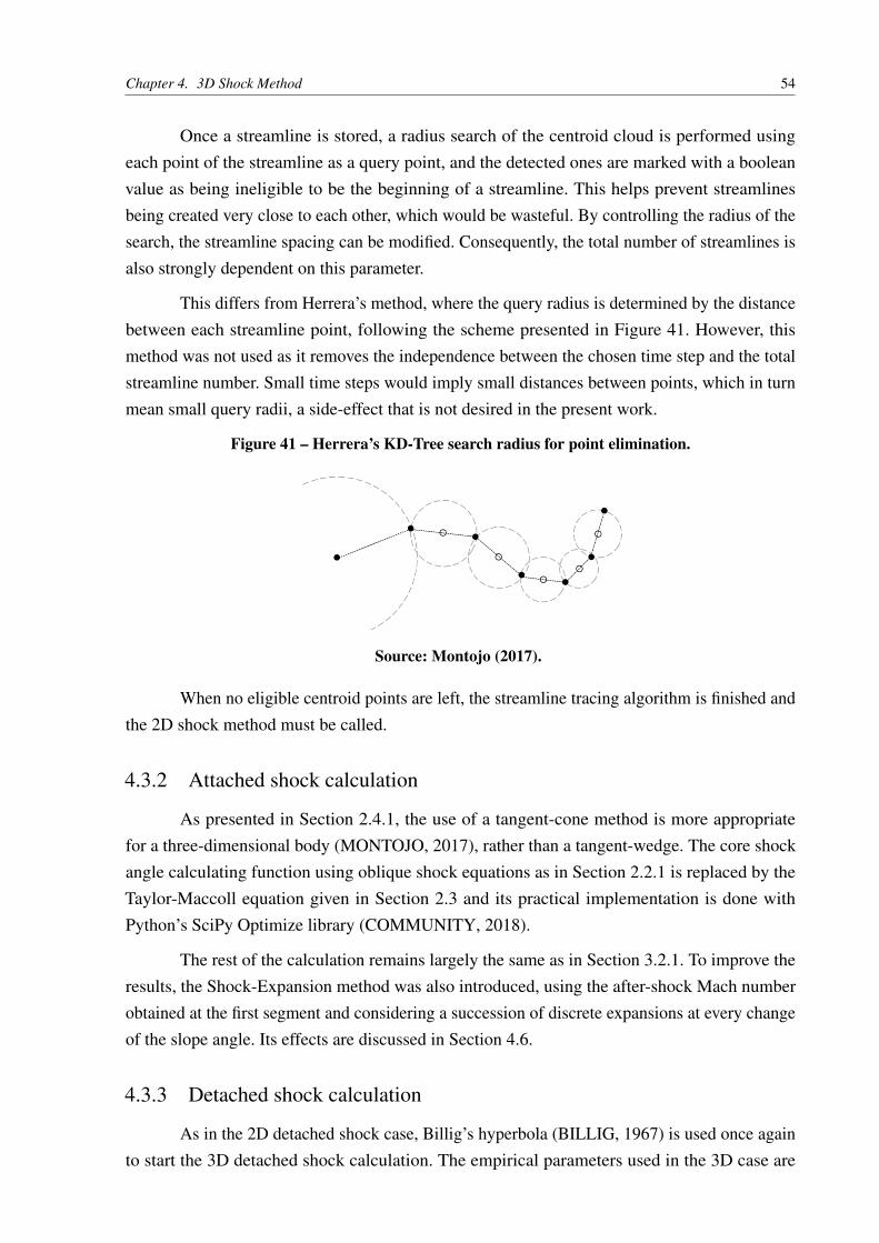
This differs from Herrera’s method, where the query radius is determined by the distancebetween each streamline point, following the scheme presented in Figure 41. However, thismethod was not used as it removes the independence between the chosen time step and the totalstreamline number. Small time steps would imply small distances between points, which in turnmean small query radii, a side-effect that is not desired in the present work.
Figure 41 – Herrera’s KD-Tree search radius for point elimination.
Source: Montojo (2017).
When no eligible centroid points are left, the streamline tracing algorithm is finished andthe 2D shock method must be called.
4.3.2 Attached shock calculation
As presented in Section 2.4.1, the use of a tangent-cone method is more appropriatefor a three-dimensional body (MONTOJO, 2017), rather than a tangent-wedge. The core shockangle calculating function using oblique shock equations as in Section 2.2.1 is replaced by theTaylor-Maccoll equation given in Section 2.3 and its practical implementation is done withPython’s SciPy Optimize library (COMMUNITY, 2018).
The rest of the calculation remains largely the same as in Section 3.2.1. To improve theresults, the Shock-Expansion method was also introduced, using the after-shock Mach numberobtained at the first segment and considering a succession of discrete expansions at every changeof the slope angle. Its effects are discussed in Section 4.6.
4.3.3 Detached shock calculation
As in the 2D detached shock case, Billig’s hyperbola (BILLIG, 1967) is used once againto start the 3D detached shock calculation. The empirical parameters used in the 3D case are
Chapter 4. 3D Shock Method 55
given by:
∆/R = 0.143exp(3.24/M2
∞
), (4.5)
Rc/R = 1.143exp[0.54/(M∞−1)1.2] . (4.6)
The hyperbola equation Eq. 3.1 does not change.
The model is currently restricted to axisymmetrical bodies. Nevertheless, for asymmetri-cal noses, two principal curvatures k1 and k2 can be defined. For a given radius R, a spectrum oftori can be generated between a pure sphere and a pure cylinder by maintaining the maximumprincipal curvature k1 = 1/R and reducing the minimum curvature k2 from 1/R to 0. Therefore,Herrera (MONTOJO, 2017) proposes a blending between the spherical and cylindrical solutions:
ftori = fcylinder exp
ln(
fsphere
fcylinder
)λ n
, (4.7)
where λ = k1/k2 is the ratio of principal curvatures and f can be either the stand-off distanceor the curvature radius functions, and n = 0.57987417201950564 (MONTOJO, 2017). Thesecurvature estimations are performed over the mesh, preceding the streamline calculations, andcan be done with CGAL’s Estimation of Local Differential Properties of Point-Sampled Surfacespackage (POUGET; CAZALS, 2018).
This function has already been implemented in the code, but it is deactivated as asym-metrical solutions have not been fully implemented. Thus, the curvature estimation can be donedirectly on the 2D model as before, since every axisymmetrical nose tip is an umbilic point, thatis, a point where the principal curvatures are equal, hence every tangent direction is a principalcurvature direction.
4.4 3D-2D shock method interface
The 2D shock structure prediction method presented in Chapter 3 can be used with the3D algorithm, modulo some modifications.
The 2D algorithm cannot directly process a three-dimensional streamline. Its coordinatesneed to be converted from Cartesian (x,y,z) to Cylindrical (x,R,θ) coordinates:
R =√
y2 + z2 , (4.8)

Chapter 4. 3D Shock Method 56
θ = arctan(
zy
). (4.9)
The x coordinate is conserved and the radius R correspond to the y-axis coordinate ofthe 2D procedure. The θ coordinate, despite being new to the method, is bypassed by the shockcalculation but it is always registered, as this is important to determine the azimuthal position ofthe shock point during the 3D shock envelope construction.
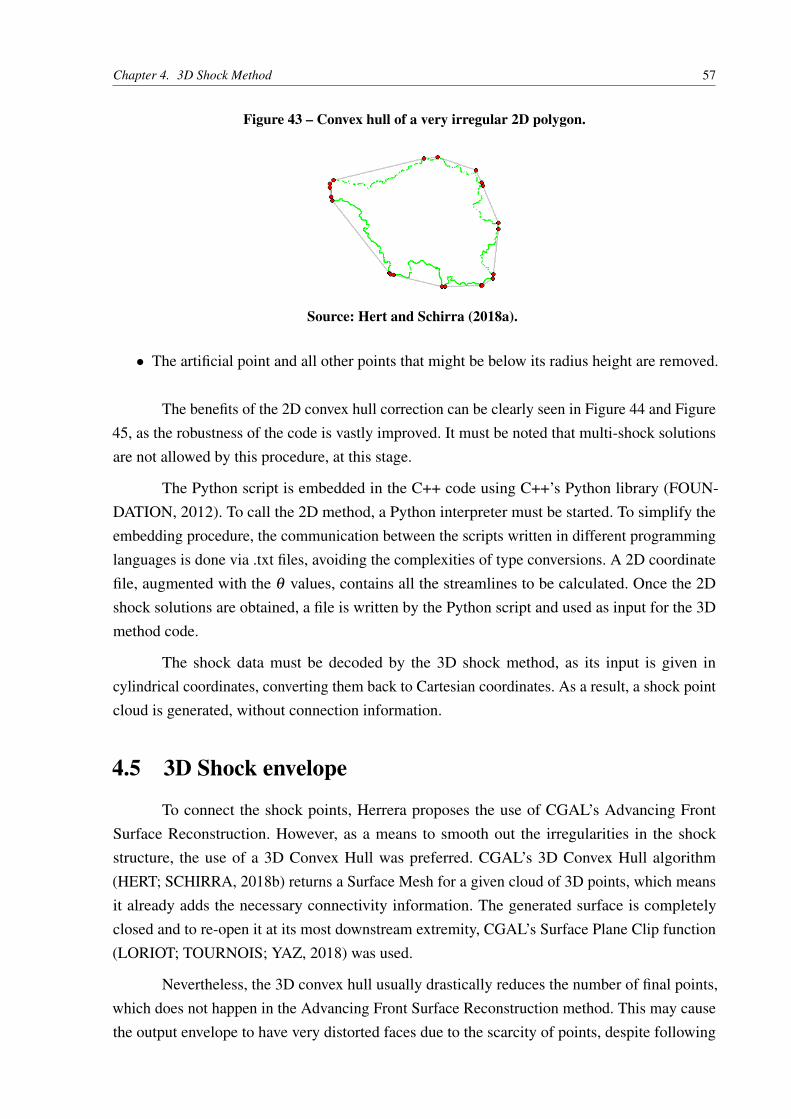
Another modification deals with the difficulty encountered in the 2D method of dealingwith irregular polylines, rendering the results completely invalid, as exemplified in Figure 42.This often happens in the integration of a streamline if the mesh is not sufficiently smooth orsimply due to its natural irregularities. The streamline is filtered with CGAL’s 2D Convex Hullalgorithm (HERT; SCHIRRA, 2018a).
Figure 42 – Errors induced by a slightly irregular 2D polyline.
Source: The author (2018).
A convex hull is mathematically defined as the smallest convex set of points that containsa given ensemble. In the two-dimensional case, it forms a polygon such as the one shown inFigure 43. Its application to smooth the polyline is as follows:
• To form a closed polygon as intended, an artificial point is added to the streamline pointvector: it is positioned with the most downstream point’s x-axis value and at the sameradius height of the most upstream point.
• The points that form the 2D convex hull are obtained from CGAL’s function.
Chapter 4. 3D Shock Method 57
Figure 43 – Convex hull of a very irregular 2D polygon.
Source: Hert and Schirra (2018a).
• The artificial point and all other points that might be below its radius height are removed.
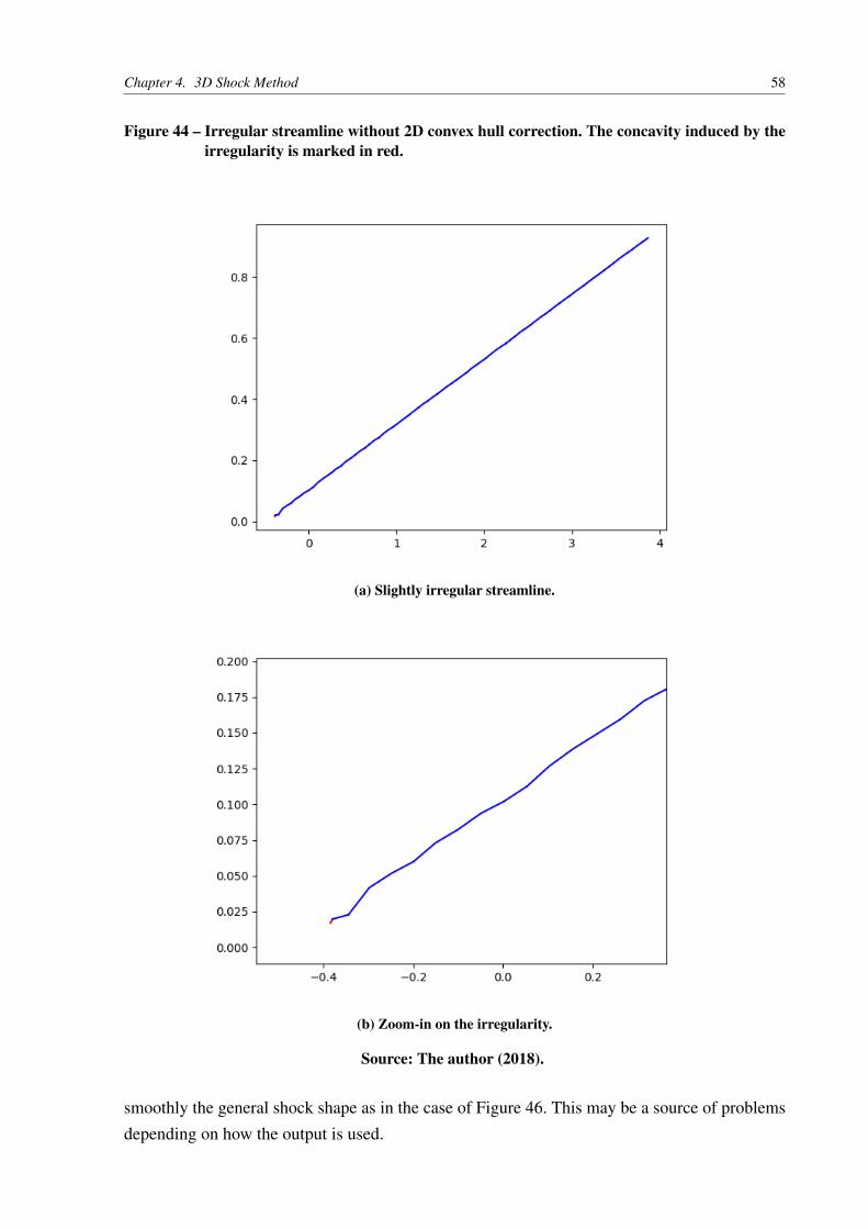
The benefits of the 2D convex hull correction can be clearly seen in Figure 44 and Figure45, as the robustness of the code is vastly improved. It must be noted that multi-shock solutionsare not allowed by this procedure, at this stage.
The Python script is embedded in the C++ code using C++’s Python library (FOUN-DATION, 2012). To call the 2D method, a Python interpreter must be started. To simplify theembedding procedure, the communication between the scripts written in different programminglanguages is done via .txt files, avoiding the complexities of type conversions. A 2D coordinatefile, augmented with the θ values, contains all the streamlines to be calculated. Once the 2Dshock solutions are obtained, a file is written by the Python script and used as input for the 3Dmethod code.
The shock data must be decoded by the 3D shock method, as its input is given incylindrical coordinates, converting them back to Cartesian coordinates. As a result, a shock pointcloud is generated, without connection information.
4.5 3D Shock envelope
To connect the shock points, Herrera proposes the use of CGAL’s Advancing FrontSurface Reconstruction. However, as a means to smooth out the irregularities in the shockstructure, the use of a 3D Convex Hull was preferred. CGAL’s 3D Convex Hull algorithm(HERT; SCHIRRA, 2018b) returns a Surface Mesh for a given cloud of 3D points, which meansit already adds the necessary connectivity information. The generated surface is completelyclosed and to re-open it at its most downstream extremity, CGAL’s Surface Plane Clip function(LORIOT; TOURNOIS; YAZ, 2018) was used.
Nevertheless, the 3D convex hull usually drastically reduces the number of final points,which does not happen in the Advancing Front Surface Reconstruction method. This may causethe output envelope to have very distorted faces due to the scarcity of points, despite following
Chapter 4. 3D Shock Method 58
Figure 44 – Irregular streamline without 2D convex hull correction. The concavity induced by theirregularity is marked in red.
(a) Slightly irregular streamline.
(b) Zoom-in on the irregularity.
Source: The author (2018).
smoothly the general shock shape as in the case of Figure 46. This may be a source of problemsdepending on how the output is used.

Chapter 4. 3D Shock Method 59
Figure 45 – Streamline with 2D convex hull correction.
(a) Fully convex streamline.
(b) Zoom-in on the correction.
Source: The author (2018).
To improve the results, CGAL’s Isotropic Re-mesher (LORIOT; TOURNOIS; YAZ,2018) was employed as seen in Figure 47. It takes the existing shock mesh given by the 3DConvex Hull and interpolates it, adding more vertices and generating facets according to the

Chapter 4. 3D Shock Method 60
Figure 46 – 3D Convex hull of a conic shock point cloud.
Source: The author (2018).
input criteria. By default, it is free to remove preexisting vertices. To avoid this, a booleanproperty map can be used to determine the mesh features that should be preserved. In this code,the preexisting vertices are prevented from being deleted, to ensure that the sharp shock featuresare protected, especially on attached shock tips.
Figure 47 – Cone shock after re-meshing the 3D convex hull.
Source: The author (2018).
4.6 3D results and analysis
In order to validate the model, some examples of three-dimensional shock structureswere generated and compared to numerical simulations, with inviscid axisymmetric conditions
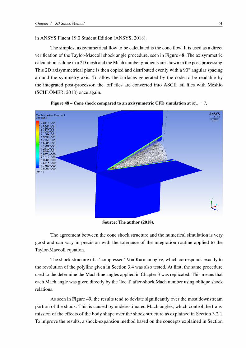
Chapter 4. 3D Shock Method 61
in ANSYS Fluent 19.0 Student Edition (ANSYS, 2018).
The simplest axisymmetrical flow to be calculated is the cone flow. It is used as a directverification of the Taylor-Maccoll shock angle procedure, seen in Figure 48. The axisymmetriccalculation is done in a 2D mesh and the Mach number gradients are shown in the post-processing.This 2D axisymmetrical plane is then copied and distributed evenly with a 90◦ angular spacingaround the symmetry axis. To allow the surfaces generated by the code to be readable bythe integrated post-processor, the .off files are converted into ASCII .stl files with Meshio(SCHLÖMER, 2018) once again.
Figure 48 – Cone shock compared to an axisymmetric CFD simulation at M∞ = 7.
Source: The author (2018).
The agreement between the cone shock structure and the numerical simulation is verygood and can vary in precision with the tolerance of the integration routine applied to theTaylor-Maccoll equation.
The shock structure of a ‘compressed’ Von Karman ogive, which corresponds exactly tothe revolution of the polyline given in Section 3.4 was also tested. At first, the same procedureused to the determine the Mach line angles applied in Chapter 3 was replicated. This means thateach Mach angle was given directly by the ‘local’ after-shock Mach number using oblique shockrelations.
As seen in Figure 49, the results tend to deviate significantly over the most downstreamportion of the shock. This is caused by underestimated Mach angles, which control the trans-mission of the effects of the body shape over the shock structure as explained in Section 3.2.1.To improve the results, a shock-expansion method based on the concepts explained in Section

Chapter 4. 3D Shock Method 62
Figure 49 – Modified Von Karman ogive compared to an axisymmetric CFD simulation at M∞ = 7.
Source: The author (2018).
2.4.2 was implemented to determine the local Mach number and consequently the Mach lineangles. This in turn yields the results given in Figure 50. The new shock prediction procedurefits slightly better than the numerical solution.
Figure 50 – Modified Von Karman ogive simulation with Shock-Expansion method at M∞ = 7.
Source: The author (2018).
A blunt cone was used in order to test the detached shock procedure. It is formed by the

Chapter 4. 3D Shock Method 63
revolution of a blunt wedge polyline as demonstrated in Figure 27. The comparison is shown inFigure 51. A correction factor has already been applied and it will be discussed in Section 4.7.
Figure 51 – Blunt cone shock compared to an axisymmetric CFD simulation at M∞ = 7.
Source: The author (2018).
The execution time of the code is in general at least 5 times faster than the axisymmetricalCFD calculation, even in complex detached cases. In attached cases, this may amount up to 10times. A precise analysis cannot be performed at this stage because it requires the determinationof an optimal streamline distribution and the adjustment of integration tolerances and time steps.The CFD overhead is evidently highly dependent on the size of its mesh elements. The authorexpects that the benefits will become much more evident in asymmetric situations, where a fullythree-dimensional numerical simulation would be necessary and its computational costs aremuch steeper.
4.7 3D model limitations
At the conclusion of this present work, the model was still limited to axisymmetricalshocks with no concave sections. This is elaborated extensively in Chapter 5.1. Focusing onthis axisymmetrical model, there are still a number of complex situations to be dealt with andimproved.
As the 2D shock model is almost entirely inserted in the 3D method with small modifica-tions, most limitations of the former are automatically carried over to the latter. This includesslope discontinuity and non-circular nose tip problems, detailed in Section 3.5.
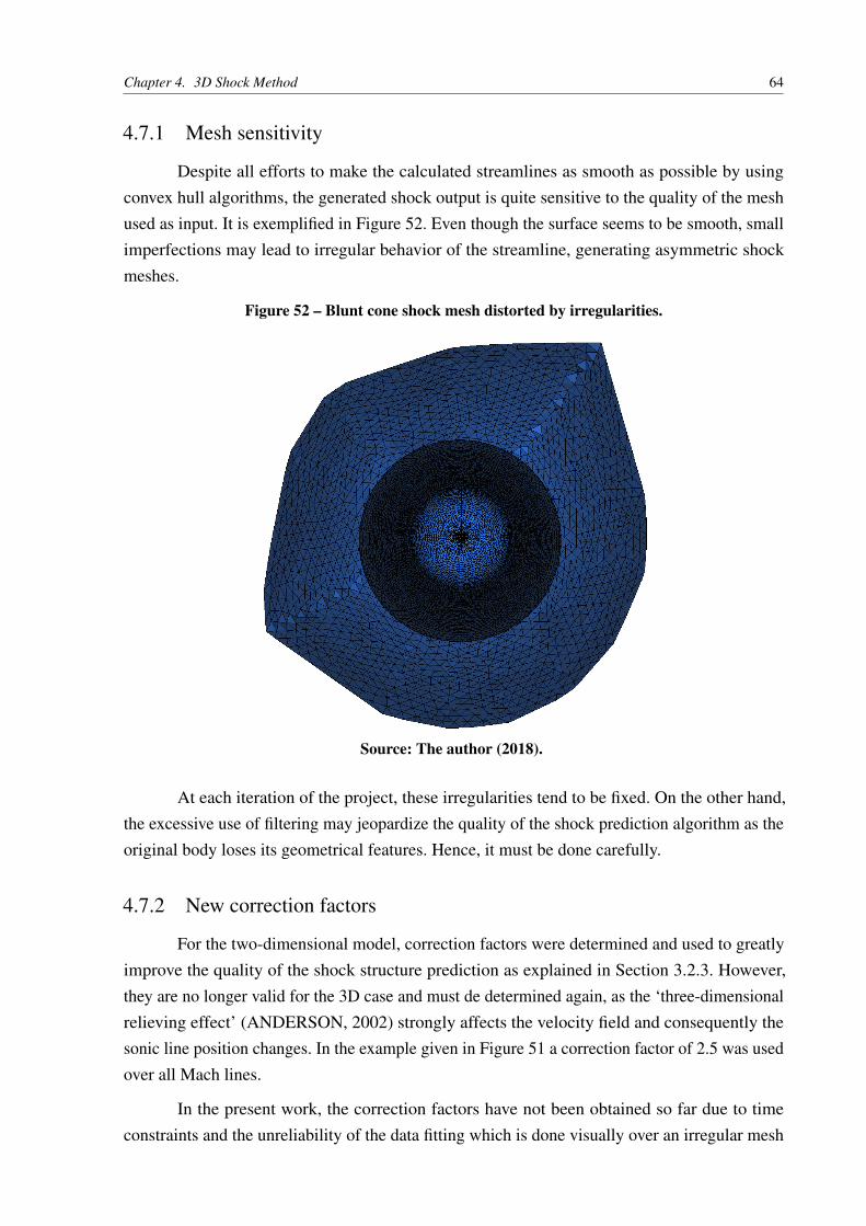
Chapter 4. 3D Shock Method 64
4.7.1 Mesh sensitivity
Despite all efforts to make the calculated streamlines as smooth as possible by usingconvex hull algorithms, the generated shock output is quite sensitive to the quality of the meshused as input. It is exemplified in Figure 52. Even though the surface seems to be smooth, smallimperfections may lead to irregular behavior of the streamline, generating asymmetric shockmeshes.
Figure 52 – Blunt cone shock mesh distorted by irregularities.
Source: The author (2018).
At each iteration of the project, these irregularities tend to be fixed. On the other hand,the excessive use of filtering may jeopardize the quality of the shock prediction algorithm as theoriginal body loses its geometrical features. Hence, it must be done carefully.
4.7.2 New correction factors
For the two-dimensional model, correction factors were determined and used to greatlyimprove the quality of the shock structure prediction as explained in Section 3.2.3. However,they are no longer valid for the 3D case and must de determined again, as the ‘three-dimensionalrelieving effect’ (ANDERSON, 2002) strongly affects the velocity field and consequently thesonic line position changes. In the example given in Figure 51 a correction factor of 2.5 was usedover all Mach lines.
In the present work, the correction factors have not been obtained so far due to timeconstraints and the unreliability of the data fitting which is done visually over an irregular mesh

Chapter 4. 3D Shock Method 65
such as the one shown in Figure 52.
66
5 CONCLUSIONS
5.1 Suggestions for future work
As presented in Sections 3.5 and 4.7, there are clear limitations in these models that canbe improved.
In the two-dimensional model, the introduction of an analytical model of expansion andshock interaction (LI; BEN-DOR, 1996) could be implemented to improve the results wherethere is a sudden slope change. This was attempted in the present work, but it was ultimatelyleft out due to the lack of real improvement. Slope discontinuities are quite rare in these designsbut it still is a concern as it can be produced in optimization geometry generation when it is notpenalized accordingly.
A more crucial problem identified in the 2D method is its incapability of treating non-circular noses. Even a simple wedge with a large half angle cannot be analyzed. A solution isalso proposed in Section 3.5, by using a weighted average of the nose radius data. It is a complexproblem and would require many CFD simulations as it is an oversimplification of the subsonicflow field effects. Nevertheless, its solution could prove to be very useful. A reliable sonic lineprediction procedure would also be invaluable.
The three-dimensional models have to be expanded to be able to handle asymmetricalshocks before they can be really applied in preliminary design. For this problem, a method isgiven by Herrera (MONTOJO, 2017), consisting of using tangent elliptical cones based on thelocal curvature properties.
Real designs often present concavities and their correct treatment in 3D models is veryimportant as mentioned in Chapter 1. Although this current model could allow multiple shocksolutions as it is already present in the 2D method, the final convex hull of shock points would notbe able to account for each shock separately. Once again, Herrera (MONTOJO, 2017) proposesthe use of machine learning methods to identify new stagnation points and effectively separatethe shocks.
In general, further analyses have still to be performed and a series of closely controlledoptimizations could help the discovery of other limitations as it could naturally yield non-conventional bodies.
5.2 Final thoughts
The goal of the present work was to analyze and improve the current shock structureestimation methodologies. Although the model is still a work in progress, it is already possibleto use it to calculate many complex shapes for engineering education purposes which would

Chapter 5. Conclusions 67
otherwise require numerical solutions and the associated resources.
After completing the method with the features mentioned in the previous section andperforming more quantitative analyses, the author believes that this method could prove to be apowerful tool in multidisciplinary design optimizations especially when multi-fidelity techniquesare used. The amount of computational resources spared could be very significant.
Throughout the development of the code and the preparation of this document, a pragmat-ical notion geared towards their application in optimization contexts was conserved. The inputsused in the program were purposefully pushed to extreme, unusual situations, irregularities wereinduced in meshes and robustness was a primary concern.
All the present work, except for the numerical simulations, relied solely on open-sourcesolutions. The CFD program was used only as a verification tool and an open-source code suchas OpenFOAM (LTD, 2018) could have been used without any loss of generality. This reinforcesthe importance and benefits of research collaborations within the scientific community.

68
BIBLIOGRAPHY
ALLIEZ, P.; TAYEB, S.; WORMSER, C. 3D fast intersection and distance computation.In: CGAL User and Reference Manual. 4.13. CGAL Editorial Board, 2018. Available at:<https://doc.cgal.org/4.13/Manual/packages.html#PkgAABB_treeSummary>.
ANDERSON, J. D. Modern Compressible Flow: with historical perspective. 3. ed. [S.l.]:McGraw-Hill Higher Education, 2002.
ANDERSON, J. D. Hypersonic and High Temperature Gas Dynamics. 2. ed. [S.l.]:American Institute of Aeronautics and Astronautics - AIAA, 2006.
ANISIMOV, D. et al. 2D generalized barycentric coordinates. In: CGAL Userand Reference Manual. 4.13. CGAL Editorial Board, 2018. Available at: <https://doc.cgal.org/4.13/Manual/packages.html#PkgBarycentric_coordinates_2Summary>.
ANSYS, I. ANSYS Free Student Software Downloads. 2018. Available at: <https://www.ansys.com/academic/free-student-products>. Accessed on: 03 may 2018.
BILLIG, F. S. Shock-wave shapes around spherical and cylindrical- nosed bodies. Journal ofSpacecraft and Rockets 4.6, American Institute of Aeronautics and Astronautics - AIAA, p.822–823, 1967.
BLANCO, J. L.; RAI, P. K. Nanoflann: a C++ Header-only Fork of FLANN,a Library for Nearest Neighbor (NN) with KD-trees. [S.l.], 2014. Available at:<https://github.com/jlblancoc/nanoflann>. Accessed on: 22 july 2018.
BOTSCH, M. et al. Surface mesh. In: CGAL User and Reference Manual. 4.13. CGALEditorial Board, 2018. Available at: <https://doc.cgal.org/4.13/Manual/packages.html#PkgSurfaceMeshSummary>.
COMMONS, W. Spherically Blunted Cone Geometry. 2009. File: Spherically bluntedcone geometry.svg. Available at: <https://commons.wikimedia.org/wiki/File:Spherically_blunted_cone_geometry.svg>. Accessed on: 22 july 2018.
COMMONS, W. Vertex Normals. 2012. File: Vertex normals.png. Available at:<https://commons.wikimedia.org/wiki/File:Vertex_normals.png>. Accessed on:22 july 2018.
COMMUNITY, T. S. Optimization and root finding. In: SciPy v1.1.0 Reference Guide. [s.n.],2018. Available at: <https://docs.python.org/3.1/extending/embedding.html>.
COMPANY, H. . What’s New in Autodesk Simulation CFD 2015. 2015. Available at: <https://hagermantechblog.wordpress.com/2014/06/30/whats-new-in-autodesk-simulation-cfd-2015/>.Accessed on: 22 july 2018.
DA, T. K. F.; COHEN-STEINER, D. Advancing front surface reconstruction. In: CGAL Userand Reference Manual. 4.13. CGAL Editorial Board, 2018. Available at: <https://doc.cgal.org/4.13/Manual/packages.html#PkgAdvancingFrontSurfaceReconstructionSummary>.
DING, F. et al. Novel approach for design of a waverider vehicle generated from axisymmetricsupersonic flows past a pointed von karman ogive. Aerospace Science and Technology, v. 42,02 2015.

Bibliography 69
EFUNDA. Circle Circumscribing a Triangle. 2018. Available at: <http://www.efunda.com/math/areas/triangleinscribedcirclegen.cfm>. Accessed on: 22 july 2018.
FOUNDATION, T. P. S. Embedding python in another application. In: Python v3.1.5 ReferenceGuide. [s.n.], 2012. Available at: <https://docs.python.org/3.1/extending/embedding.html>.
FREY, P. J. MEDIT: An interactive mesh visualization software. 2001. Available at:<https://www.ljll.math.upmc.fr/frey/publications/RT-0253.pdf>. Accessed on: 22 july 2018.
HALIR, R.; FLUSSER, J. Numerically Stable Direct Least Squares Fitting of Ellipses.1999.
HEPLER, A. K. et al. A Turbojet-Boosted Two-Stage-to-Orbit Space TransportationSystem Design Study - NASA Contractor Report 159018. Hampton, The United States:[s.n.], 1979.
HERT, S.; SCHIRRA, S. 2D convex hulls and extreme points. In: CGAL Userand Reference Manual. 4.13. CGAL Editorial Board, 2018. Available at: <https://doc.cgal.org/4.13/Manual/packages.html#PkgConvexHull2Summary>.
HERT, S.; SCHIRRA, S. 3D convex hulls. In: CGAL User and Reference Manual. 4.13.CGAL Editorial Board, 2018. Available at: <https://doc.cgal.org/4.13/Manual/packages.html#PkgConvexHull3Summary>.
LI, H.; BEN-DOR, G. Oblique-shock/expansion-fan interaction - analytical solution. AiaaJournal - AIAA J, v. 34, p. 418–421, 02 1996.
LORIOT, S.; TOURNOIS, J.; YAZ, I. O. Polygon mesh processing. In: CGALUser and Reference Manual. 4.13. CGAL Editorial Board, 2018. Available at:<https://doc.cgal.org/4.13/Manual/packages.html#PkgPolygonMeshProcessingSummary>.
LTD, O. OpenFOAM: The Open Source CFD Toolbox. 2018. Available at: <https://www.openfoam.com/>. Accessed on: 03 may 2018.
MONTOJO, J. H. Shock Estimation in Supersonic Vehicles. Phd Thesis (PhD Thesis) —University of Strathclyde, Glasgow, Scotland, 2017.
NACA, N. A. C. for A. NACA Technical Report 1135: Equations, Tables, and Charts forCompressible Flow. NACA AMES Aeronautical Laboratory: [s.n.], 1953.
ONERA, O. national d’études et de recherches aérospatiales. About ONERA - Identity. 2018.Available at: <https://www.onera.fr/en/identity>. Accessed on: 24 july 2018.
POUGET, M.; CAZALS, F. Estimation of local differential properties of point-sampled surfaces.In: CGAL User and Reference Manual. 4.13. CGAL Editorial Board, 2018. Available at:<https://doc.cgal.org/4.13/Manual/packages.html#PkgJet_fitting_3Summary>.
PROJECT, B. Boost C++ Libraries. 2018. Available at: <https://www.boost.org/>. Accessedon: 22 july 2018.
RANDALL, J. Azure From the Trenches: Introductory Guide to AABB TreeCollision Detection. 2018. Available at: <https://www.azurefromthetrenches.com/introductory-guide-to-aabb-tree-collision-detection/>. Accessed on: 22 july 2018.

Bibliography 70
SCHLÖMER, N. Meshio Mesh Format Converter. 2018. Available at: <https://github.com/nschloe/meshio>. Accessed on: 22 july 2018.
The CGAL Project. CGAL User and Reference Manual. 4.13. CGAL Editorial Board, 2018.Available at: <https://doc.cgal.org/4.13/Manual/packages.html>.
TYNER, B. KD Trees. 2006. Available at: <http://www.stat.purdue.edu/~btyner/packages.html>.Accessed on: 22 july 2018.
WATTS, J. D. NASA Technical Memorandum TM X-1669. Washington D.C., The UnitedStates: [s.n.], 1968.
ZINIU, W. et al. Review of shock wave detection method in cfd post-processing. ChineseJournal of Aeronautics, v. 26, 05 2013.