Development of Enhanced Pavement Deterioration Curves · amec foster wheeler ... development of enhanced pavement deterioration curves ... development of enhanced pavement deterioration

Development of Enhanced Pavement Deterioration Curves

http://www.virginiadot.org/vtrc/main/online_reports/pdf/17-r7.pdf SAMER W. KATICHA, Ph.D., Senior Research Associate, Center for Sustainable Transportation Infrastructure, Virginia Tech Transportation Institute, Virginia Tech SAFAK ERCISLI, Transportation Engineer, Leidos GERARDO W. FLINTSCH, Ph.D., P.E., Director, Center for Sustainable Transportation Infrastructure, Virginia Tech Transportation Institute, and Professor, Charles E. Via, Jr. Department of Civil and Environmental Engineering, Virginia Tech JAMES M. BRYCE, Ph.D., Senior Consultant, Amec Foster Wheeler BRIAN K. DIEFENDERFER, Ph.D., P.E., Associate Principal Research Scientist, Virginia Transportation Research Council

Final Report VTRC 17-R7

Standard Title Page—Report on State Project

Report No.:

VTRC 17-R7

Report Date:

October 2016

No. Pages:

38

Type Report:

Final Contract

Project No.:

105332

Period Covered:

Contract No.:

Title:

Development of Enhanced Pavement Deterioration Curves

Key Words: pavement, service life,

structural condition

Author(s):

Samer W. Katicha, Ph.D., Safak Ercisli, Gerardo W. Flintsch, Ph.D., P.E., James M.

Bryce, Ph.D., and Brian K. Diefenderfer, Ph.D., P.E.

Performing Organization:

Virginia Tech Transportation Institute

3500 Transportation Research Way

Blacksburg, VA 24061

Virginia Transportation Research Council

530 Edgemont Rd

Charlottesville, VA 22903

Sponsoring Agencies’ Name and Address:

Virginia Department of Transportation

1401 E. Broad Street

Richmond, VA 23219

Supplementary Notes:

Abstract:

This report describes the research performed by the Center for Sustainable Transportation Infrastructure (CSTI) at the

Virginia Tech Transportation Institute (VTTI) to develop a pavement condition prediction model, using (negative binomial)

regression, that takes into account pavement age and pavement structural condition expressed in terms of the Modified Structural

Index (MSI). The MSI was found to be a significant input parameter that affects the rate of deterioration of a pavement section

with the Akaike Information Criterion (AIC) suggesting that the model that includes the MSI is, at least, 50,000 times more likely

to be closer to the true model than the model that does not include the MSI. For a typical pavement at 7 years of age (since the

last rehabilitation), the effect of reducing the MSI from 1 to 0.6 results in reducing the critical condition index (CCI) from 79 to

70.

The developed regression model predicts the average CCI of pavement sections for a given age and MSI value. In

practice, the actual CCI of specific pavement sections will vary from the model-predicted condition because many (important)

factors that affect deterioration are not considered in the model. Therefore an empirical Bayes (EB) method is proposed to better

estimate the CCI of a specific pavement section. The EB method combines the recorded CCI of the specific section with the CCI

predicted from the model using a weighted average that depends on the variability of individual pavement sections performance

and the variability of CCI measurements. This approach resulted in improving the prediction of the future CCI, calculated using

leave one out cross validation, by 21.6%.

FINAL REPORT

DEVELOPMENT OF ENHANCED PAVEMENT DETERIORATION CURVES

Samer W. Katicha, Ph.D.

Senior Research Associate

Center for Sustainable Transportation Infrastructure


Virginia Tech

Safak Ercisli

Transportation Engineer

Leidos

Gerardo W. Flintsch, Ph.D., P.E.

Director



and

Professor

Charles E. Via, Jr. Department of Civil and Environmental Engineering

Virginia Tech

James M. Bryce, Ph.D.

Senior Consultant

Amec Foster Wheeler

Brian K. Diefenderfer, Ph.D., P.E.

Associate Principal Research Scientist


VTRC Project Manager




(A partnership of the Virginia Department of Transportation

and the University of Virginia since 1948)

Charlottesville, Virginia

October 2016

VTRC 17-R7

ii

DISCLAIMER

The project that is the subject of this report was done under contract for the Virginia

Department of Transportation, Virginia Transportation Research Council. The contents of this

report reflect the views of the author(s), who is responsible for the facts and the accuracy of the

data presented herein. The contents do not necessarily reflect the official views or policies of the

Virginia Department of Transportation, the Commonwealth Transportation Board, or the Federal

Highway Administration. This report does not constitute a standard, specification, or regulation.

Any inclusion of manufacturer names, trade names, or trademarks is for identification purposes

only and is not to be considered an endorsement.

Each contract report is peer reviewed and accepted for publication by staff of Virginia

Transportation Research Council with expertise in related technical areas. Final editing and

proofreading of the report are performed by the contractor.

Copyright 2016 by the Commonwealth of Virginia.

All rights reserved.

iii

ABSTRACT

This report describes the research performed by the Center for Sustainable Transportation

Infrastructure (CSTI) at the Virginia Tech Transportation Institute (VTTI) to develop a pavement

condition prediction model, using (negative binomial) regression, that takes into account

pavement age and pavement structural condition expressed in terms of the Modified Structural

Index (MSI). The MSI was found to be a significant input parameter that affects the rate of

deterioration of a pavement section with the Akaike Information Criterion (AIC) suggesting that

the model that includes the MSI is, at least, 50,000 times more likely to be closer to the true

model than the model that does not include the MSI. For a typical pavement at 7 years of age

(since the last rehabilitation), the effect of reducing the MSI from 1 to 0.6 results in reducing the

critical condition index (CCI) from 79 to 70.

The developed regression model predicts the average CCI of pavement sections for a

given age and MSI value. In practice, the actual CCI of specific pavement sections will vary

from the model-predicted condition because many (important) factors that affect deterioration

are not considered in the model. Therefore an empirical Bayes (EB) method is proposed to

better estimate the CCI of a specific pavement section. The EB method combines the recorded

CCI of the specific section with the CCI predicted from the model using a weighted average that

depends on the variability of individual pavement sections performance and the variability of

CCI measurements. This approach resulted in improving the prediction of the future CCI,

calculated using leave one out cross validation, by 21.6%.

1

FINAL REPORT

DEVELOPMENT OF ENHANCED PAVEMENT DETERIORATION CURVES

Samer W. Katicha, Ph.D.

Senior Research Associate



Virginia Tech

Safak Ercisli

Transportation Engineer

Leidos

Gerardo W. Flintsch, Ph.D., P.E.

Director



and

Professor

Charles E. Via, Jr. Department of Civil and Environmental Engineering

Virginia Tech

James M. Bryce, Ph.D.

Senior Consultant

Amec Foster Wheeler


Associate Principal Research Scientist


INTRODUCTION

One of the main goals of the Virginia Department of Transportation (VDOT) is to keep

the entire road network operating at a high serviceability level. Accurate pavement performance

prediction can significantly help pavement managers achieve that goal. Current pavement

performance prediction models (also called deterioration models or deterioration curves) used by

VDOT do not directly take into account how the pavement structural condition affects pavement

performance. This will result in less than optimal decisions as research has shown that the

pavement structural condition significantly affects the pavement performance (Bryce et al., 2013;

Flora, 2009; and Zaghloul et al., 1998). In 2007, Stantec Consulting Services Inc. with the

cooperation of H.W. Lochner Inc., henceforth referred to as Stantec, developed default pavement

deterioration models for VDOT. The practice within VDOT is to use two types of performance

prediction models: site specific models where sufficiently accurate site specific data are available

2

and default models where such accurate data are not available. Data accuracy is determined

through quality checks that predict the minimum and maximum service life, which are compared

with a pre-defined range of acceptance.

Although the pavement structural condition was not directly incorporated in the default

deterioration models developed by Stantec, it was recognized that different pavement

rehabilitation treatments have different effects on the pavement structural condition and hence

future performance. Therefore, different default deterioration models were developed for the

different pavement rehabilitation treatments. These rehabilitation treatments are grouped into

four maintenance categories namely, preventive maintenance (PM), corrective maintenance

(CM), restorative maintenance (RM), and reconstruction (RC). In summary, the approach

followed by Stantec was to use the windshield pavement survey data and develop pavement

performance models assuming all pavement sections had CM as a last treatment. The assumption

of a last treatment was necessary as the windshield data did not record the type of the last

treatment. Expert opinion from within VDOT was then combined with the developed model for

CM to develop models for the remaining three maintenance categories (Stantec, 2007).

PURPOSE AND SCOPE

Purpose

The main purpose of this study was to develop a pavement deterioration regression model

for bituminous sections of VDOT Interstate roads that take into account the pavement structural

condition. The developed regression model can be implemented by VDOT in their pavement

management system (PMS) to better account for the effect of structural condition on pavement

performance.

The pavement structural condition accounts for some (significant) but not all of the

variability of the performance of the pavement sections. Therefore, a methodology that

combines the model predicted Critical Condition Index (CCI) with the measured CCI to account

for the unexplained variability by the model is also presented and validated by (leave-one-out)

cross validation. This additional step can be implemented separately from the regression.

Scope

The data used in this project were obtained from the Interstate roads in Virginia. This

restriction was necessary because the primary and secondary roads in the VDOT network do not

have network level structural evaluation measurements. A key aspect of this study was to adopt a

model for the pavement deterioration process that can explain the observed data. The study

found that a Negative Binomial model provides a good representation of the observed pavement

condition (and much better representation than a model based on the normal distribution). In

addition to providing a good fit to the observed data, which will result in a better regression

model, the Negative Binomial model can also take into account the fact that variation in the

3

observed pavement condition comes from two sources. The first source is variation in

performance of different pavement sections while the second source is variation due to

variability in the measurement and reporting of the pavement condition.

With these two sources of variations, an empirical Bayes (EB) approach that combines

the pavement performance model obtained from the Negative Binomial regression with the

condition of individual pavement sections is used to estimate the performance of each pavement

section. This estimate is better than what is separately achieved by either the model or the actual

observations.

METHODS

There are two products from this research. The first main product is the regression model

that estimates the pavement CCI based on age and MSI, which is the ratio or effective structural

number (SNeff) over required structural number (SNreq). SNeff is calculated from falling weight

deflectometer (FWD) data while SNreq is calculated based on the AASHTO 1993 design method

for flexible pavements (see Bryce et al., 2013 for more details). The second product is the EB

estimate of CCI that combines the model predicted CCI with the measured CCI to provide an

improved estimate of the CCI.

The first product of this research, the regression model, was developed as follows:

1. From the recorded CCI, calculate the Deterioration Index (DI) as follows:

CCIDI 100 (1)

2. Using the DI, pavement age T, and MSI, perform a negative binomial regression to

determine the relationship between DI and T, and MSI. The regression provides an

estimate modelDI of DI. The modelCCI can then be calculated from modelDI . The form

is given in Equation 3.

T

MSITT

MSI eTeDI3410

232410

1ln

1

model

(2)

T

MSITT

MSI eTeDICCI3410

232410

1ln

1

modelmodel 100100100

(3)

The chosen model includes two terms for the pavement age T. The first term, ln(T),

is included so that at T = 0, the resulting deterioration is zero (i.e., DI = 0 and CCI =

100). The second term, T, is included because it was found that adding T results in

the model having a typical observed shape of pavement deterioration (with just ln(T)

the shape of the deterioration obtained from the model is not typical of observed

pavement deterioration). In the end, adding the term T was also found to be

statistically justifiable as it significantly improved the model fit.

4

The second product of this research was to combine DI with modelDI to give a better

estimate EBDI and EBCCI and determine the future pavement condition. This is performed as

follows

1. DI and modelDI are combined to give EBDI using Equation 4, which is the EB

approach of combining observation with model estimate:

DI

DI

DI

DI

DIEB

1

11

1

1

model

model

model

(4)

2. EBCCI , is then obtained using Equation 5:

EBEB DICCI 100 (5)

3. The estimate of the following year’s condition (if no observation is available) can be

obtained by estimating the pavement deterioration calculated using the developed

model as shown in Equation 6:

iii

EB

i

EB CCICCICCICCI model

1

model

1 (6)

In Equations 2 and 3, MSI refers to the Modified Structural Index developed by Bryce et

al. (2013), T, the pavement age (since last treatment). The regression coefficients were calculated

as β0, β1, β2 and, β3. In Equation 3, is a (overdispersion) parameter also obtained from the

model regression, while α is a variance correction parameter that accounts for the deviations of

the pavement condition data from the theoretical modeling procedure. All these parameters were

determined using the pavement condition data. An example EB calculation is in Appendix A.

This methodology was followed because it is more appropriate for the condition data of

pavement sections. The reason it is more appropriate was justified as follows:

1. Use of Negative Binomial distribution and regression: the empirical distribution of DI

(100 – CCI) values obtained from the PMS was evaluated and found to be better

represented by a Negative Binomial distribution than a normal distribution.

2. Including MSI in the regression model: the Akaike Information Criterion (AIC) was

used to validate the model, mainly to justify including the pavement structural

condition along with pavement age as one of the parameters that determines

pavement condition. Adding regression variables always improves the fit of the

model. The AIC penalizes the addition of regression variables so that only

statistically significant variables are included.

5

3. Use of the variance correction parameter α: The Negative Binomial model results

from a Poisson-Gamma model where the Gamma distribution represents the

variability of the deterioration of different pavement sections while the Poisson

distribution represents the variability in reporting of the pavement condition (error in

the measured DI or CCI). It was found that the Poisson distribution underestimates

the variability in the reporting of the pavement condition, which justified the

inclusion of the variance correction parameter α. However, the Poisson distribution

predicts that the variance of the reporting of the pavement condition is equal to the

DI. This implies a linear relationship with a slope of unity. Similarly, the data

showed that the variance is linearly related to the DI but with a slope of α instead of

unity.

4. Validate the use of the EB approach: the EB approach was validated using leave-one-

out cross validation, which consists of leaving one observation out of the model

building and then predicting the condition for the observation that was left out. This

process is repeated for every observation in the data set. The model prediction

capability is estimated as the mean square prediction error and compared to the mean

square error prediction obtained without any modeling of the pavement deterioration

process.

Step 1. Data Collection and Distribution of Pavement Condition

The MSI developed in Bryce et al. (2013) was calculated from network-level FWD data

collected on the Interstate roads. The MSI data were then supplemented with the pavement CCI,

year of condition recording, and last year of maintenance data obtained from the VDOT PMS

database for the years from 2007 to 2012, 2014, and 2015. The data from the years 2007 to 2012

were those initially available when the research project started and those data were used to

develop and validate the model. The data from 2014 and 2015 became available at the end of the

research project and were incorporated into the final model. However, they were not used in the

validation of the model, as this would have required repeating the entire analysis. The MSI

incorporates the information about deflection testing, pavement thickness, and traffic. The data

were aggregated using the pavement management section currently in use. From the PMS data,

the age of the pavement was calculated as the difference between the year of condition reporting

and the last year of recorded maintenance. The total data consisted of 3,473 observations for the

years from 2007 to 2012 and 1,560 observations from the years 2014 and 2015. To evaluate the

CCI distribution, the DI, which is the complement of the CCI, was defined as shown in Equation

1. The reason DI is defined is for mathematical convenience as it was found that the DI and not

the CCI follows the Negative Binomial distribution. The probability density function of the

Negative Binomial distribution, which is also a compound Poisson-gamma distribution, is given

in Appendix B along with the Poisson and Gamma distributions.

6

Step 2. Development of Deterioration Model

Because the distribution of the pavement DI was found to be well represented by a

Negative Binomial distribution, the default pavement deterioration model was obtained using

Negative Binomial regression, which is a form of a Generalized Linear Model (GLM)

regression. Other than the fact the DI values are distributed as a Negative Binomial distribution,

one of the advantages of Negative Binomial regression is that its natural link function is the

exponential function, which was used in 2007 by Stantec to develop the default pavement

deterioration models. The final model used is given by Equation 2.

Pavement condition data consist of censored data, where censoring occurs because of

treatments applied to the pavement. This can lead to a biased deterioration model. The key idea

is to recognize that data at higher pavement ages are mostly those of pavement sections that

performed well; pavement sections that did not perform well are generally treated before

reaching an older age. As such, data at older ages do not represent the performance of all

pavement sections and are therefore biased. If not accounted for, this bias will result in a biased

pavement deterioration model. For this reason, the model was fitted to a range of pavement age

where this biasing effect is believed to be minimal. This was determined to be for data up to and

including an age of 10 years.

The model parameters were determined by maximizing the likelihood function. Because

the sections have different lengths, the maximization is done with the proper weighting (section

length) of the data. In the process of developing the model, the study investigated different linear

relationships in the exponential function. The final chosen model resulted in the best fit

(maximized the likelihood). Furthermore, taking the natural logarithm of the pavement age, T,

ensures that the DI at year zero is zero (CCI at year zero is 100), which is a desirable property.

The AIC, which penalizes adding variables to the model, was used to validate incorporating the

MSI in the model. Details of the AIC are presented in Appendix C.

Step 3. Empirical Bayes Estimate of Pavement Condition

Negative Binomial (Poisson-Gamma) Model

The Negative Binomial regression gives the coefficients of the model parameters (T,

MSI, and intercept) that, when substituted in Equation 2 give modelDI , which is the average

response of pavement sections with the same age T and MSI. Another parameter obtained from

the Negative Binomial regression is what is referred to as the overdispersion parameter, . This

parameter takes into account the variability of different pavement sections. For the Negative

Binomial model, the variance, 2

s , of the pavement sections condition can be calculated from

modelDI and as shown in Equation 7. Under the Poisson error assumption, the variance of the

error in condition reporting is equal to modelDI . One way to justify the dependence of the

variance on the pavement condition is to consider that it is easier to rate pavements in good

condition than it is to rate pavements in poor condition. This will lead to ratings of pavements in

a poorer condition having higher variability (i.e., error). This seems plausible given that there

7

are several combinations of distresses that can cause a pavement section to be in poor condition

but there is essentially one way (no distresses) for a pavement section to be in perfect condition.

The data support this observation as more variability is observed for pavement sections that are

in worse condition. Therefore, the total variance, 2

mod , of the model can be calculated as shown

in Equation 8.

2model

2 DIs (7)

modelmodel

2

mod 1 DIDI (8)

The mean, modelDI , variance, 2

mod , and overdispersion, , are related to the parameters of

the Negative Binomial model. The Poisson-Gamma model gives rise to a Bayesian model with

the Gamma distribution prior. In practical terms, modelDI is the prior, which represents the

variability of the performance of different pavement sections. Once the data, DI, are observed,

the posterior distribution of the true pavement condition, EBDI , can be calculated using Bayes’

formula. In the EB approach, the parameters of the prior are estimated from the data; in this

case, by the Negative Binomial regression. The practical interpretation of Bayes’ formula is that

it combines the (practical) experience that can be learned from observing the historical

performance of all pavement sections with specific observations to come up with an improved

estimate of the pavement condition. The information from the prior and observation are

combined using Equation 9. Note that Equation 3 is similar to Equation 9 with the added

parameter α, which is included because the observed data do not strictly follow the Poisson-

Gamma model.

DIDI

DIDI

DIEB

1

11

1

1

model

model

model (9)

Deviation from the Negative Binomial (Poisson-Gamma) Model

The EB estimate in Equation 9 assumes the measurement error for reporting the CCI

follows a Poisson distribution. The difference sequence method, which is described in Appendix

D, was used to independently evaluate the variance of the error in reporting the CCI and it was

found that this error variance is larger than what is predicted by the Poisson distribution. A

concern could then be raised towards the applicability of the EB approach since the model

assumptions, mainly Poisson error distribution, are violated. However, even if the Poisson-

Gamma model is completely incorrect, as long as the variance of the error is not significantly

overestimated, the EB estimate is still a better estimate than the actual measurement (either

current or future). This is a result of linear Bayes estimators, which guarantee that irrespective of

the true distribution of pavement performance, as well as the true distribution of the error in the

measurement of the pavement condition, the linear Bayes estimator (of which the Poisson-

Gamma model is one) improves on the estimate of the condition compared to just considering

the measurement alone (see Hartigan, 1969, and Efron, 1973). The improvement of the linear

Bayes estimator is such that the mean square error is reduced by a factor of:

8

22

2

2

mod

2

Errors

ss

(10)

If the error variance, 2

Error , is underestimated, as is the case when assuming a Poisson

error distribution, then the improvement of the EB estimate will be less than optimal. Therefore,

the EB estimate in Equation 9 is conservative and can be improved if the appropriate value for

the error variance is used. The linear EB estimator is calculated using Equation 11, which can be

used for any two distributions and without knowledge of the appropriate distribution form:

DIDIDIErrors

s

Errors

sEB 22

2

model22

2

1

(11)

Note the similarities between Equation 9 and Equation 11 and it can be shown that if 22

PoissonError (i.e., the error predicted from the Poisson distribution is different than the error

in the data), then Equation 9 can still be used with replaced by c , which is the form of

Equation 3.

Step 4. Validating the Modeling Procedure

Dependence of Error in DI Measurement on Pavement Condition

Based on the difference sequence method, it was found that the Poisson distribution

assumption underestimated the error variance of the observed data. A correction factor, α, was

used to adjust for the discrepancy as shown in Equation 12. However, since for the Poisson

distribution, the variance is equal to the mean, the measurement error was checked relative to the

average of the observation as shown in Equation 13. Finally, the total variance of the data is

related to the variance of the pavement sections’ performance and the error variance as shown in

Equation 14. The factor 2

mod is the total variance, which should be equal to the variance of the

observed data.

22

PoissonError (12)

i

i DImodel

2Error (13)

222

mod Errors (14)

Validating the Empirical Bayes Approach

The optimal test to validate a modeling procedure would be to know the actual true value

that is being estimated (here the pavement deterioration represented by either the DI or the CCI)

and verify that the chosen modeling procedure gives a better estimate of the true value compared

9

to no modeling (i.e., just using the observations). For real data, the true value is never known

and this approach cannot be followed. An alternative approach is to compare the mean square

error prediction with the criterion that the approach that results in a lower prediction error (of

measurements not used in developing the model) is a better approach. We can think of the

measurements used to estimate prediction error as measurements from future pavement surveys;

clearly being able to better predict the pavement condition in future pavement surveys (for

example next year’s survey), is a desirable quality of any model. The prediction error was

evaluated as follows:

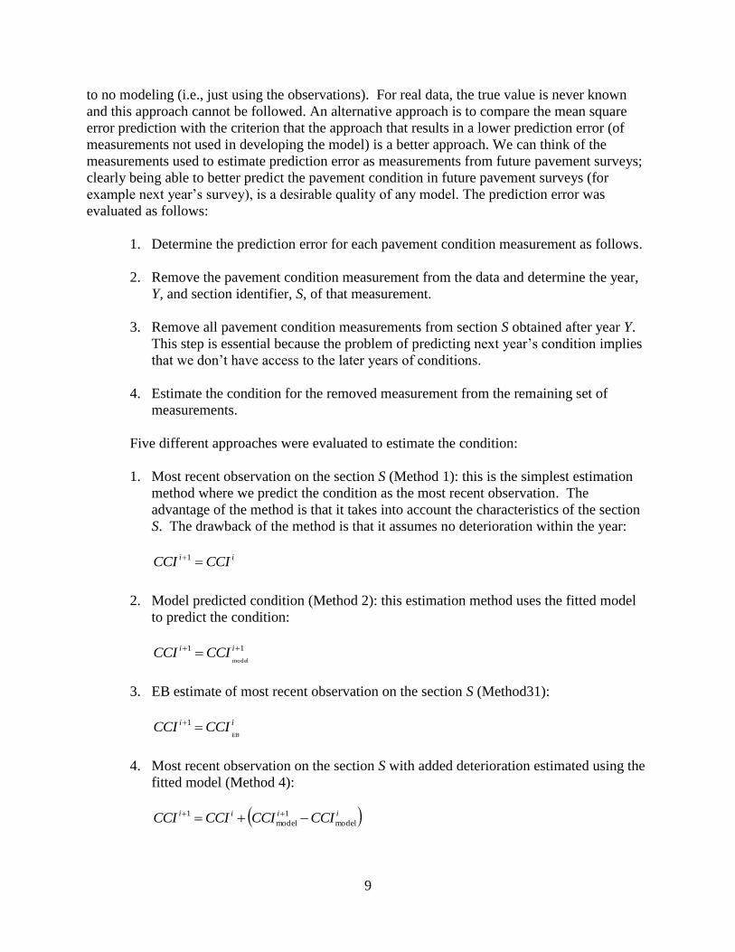
1. Determine the prediction error for each pavement condition measurement as follows.

2. Remove the pavement condition measurement from the data and determine the year,

Y, and section identifier, S, of that measurement.

3. Remove all pavement condition measurements from section S obtained after year Y.

This step is essential because the problem of predicting next year’s condition implies

that we don’t have access to the later years of conditions.

4. Estimate the condition for the removed measurement from the remaining set of

measurements.

Five different approaches were evaluated to estimate the condition:

1. Most recent observation on the section S (Method 1): this is the simplest estimation

method where we predict the condition as the most recent observation. The

advantage of the method is that it takes into account the characteristics of the section

S. The drawback of the method is that it assumes no deterioration within the year:

ii CCICCI 1

2. Model predicted condition (Method 2): this estimation method uses the fitted model

to predict the condition:

11

model

ii CCICCI

3. EB estimate of most recent observation on the section S (Method31):

ii

EBCCICCI 1

4. Most recent observation on the section S with added deterioration estimated using the

fitted model (Method 4):

iiii CCICCICCICCI model

1

model

1

10

5. EB estimate of most recent observation on the section S with added deterioration

estimated using the fitted model (Method 5):

iii

EB

i

EB CCICCICCICCI model

1

model

1

RESULTS AND DISCUSSION

Step 1. Data Collection and Distribution of Pavement Condition

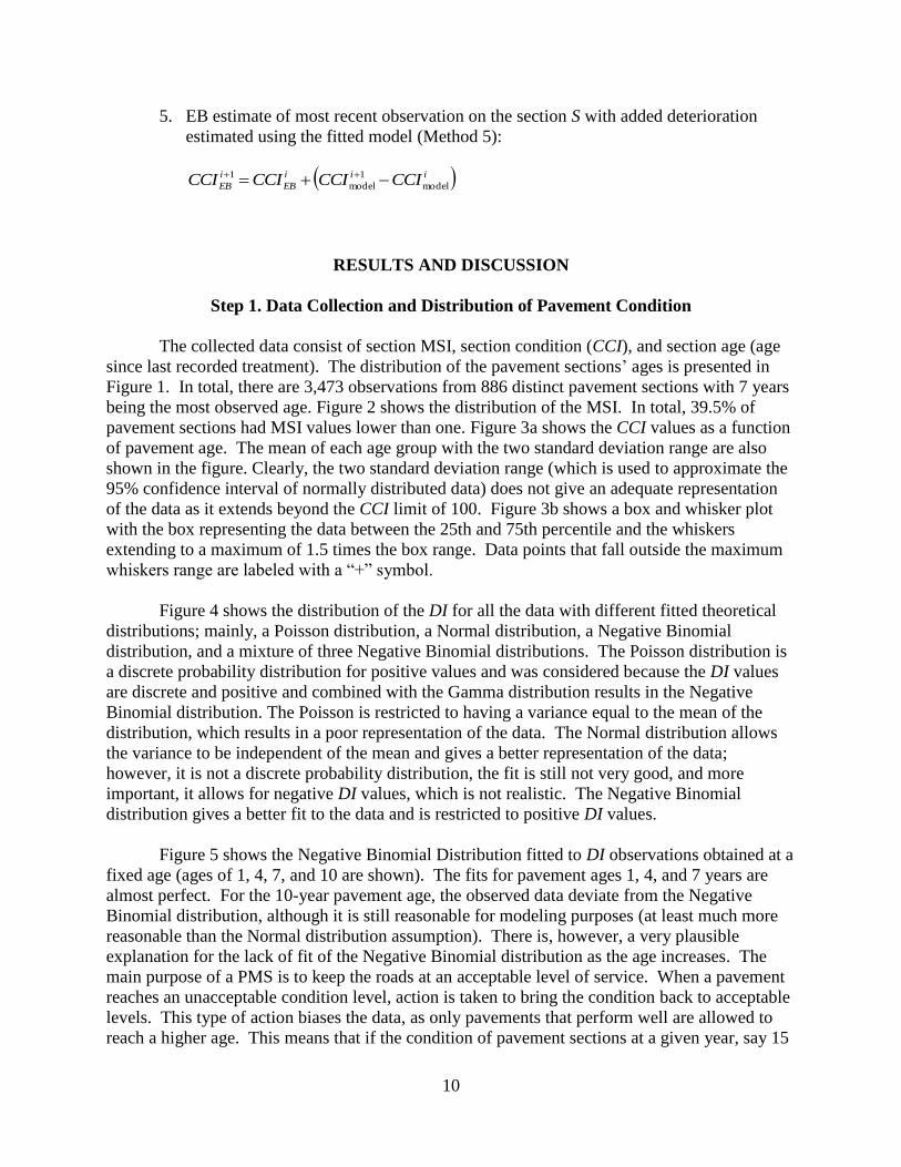
The collected data consist of section MSI, section condition (CCI), and section age (age

since last recorded treatment). The distribution of the pavement sections’ ages is presented in

Figure 1. In total, there are 3,473 observations from 886 distinct pavement sections with 7 years

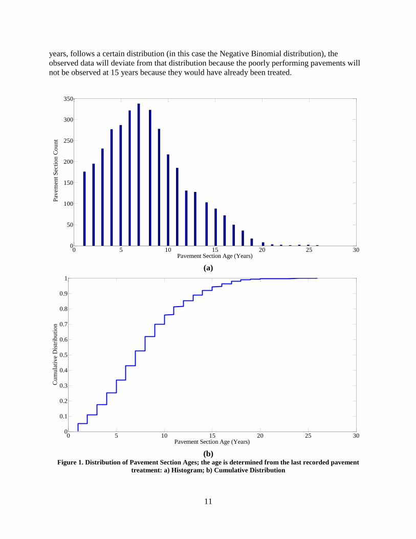
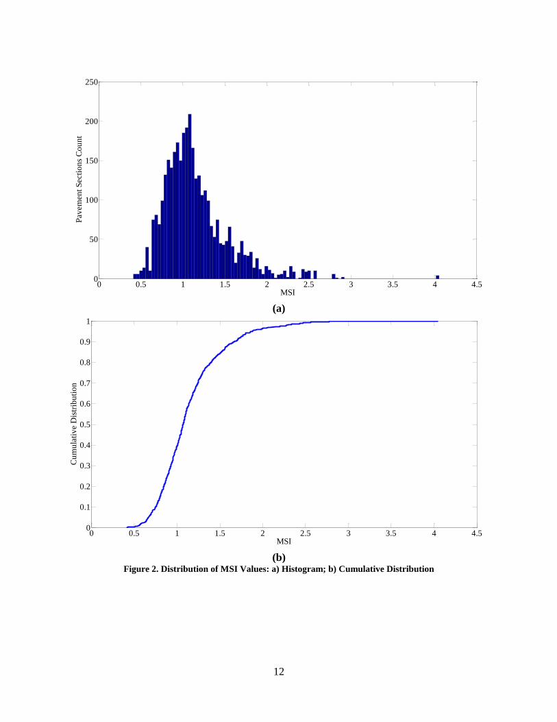
being the most observed age. Figure 2 shows the distribution of the MSI. In total, 39.5% of

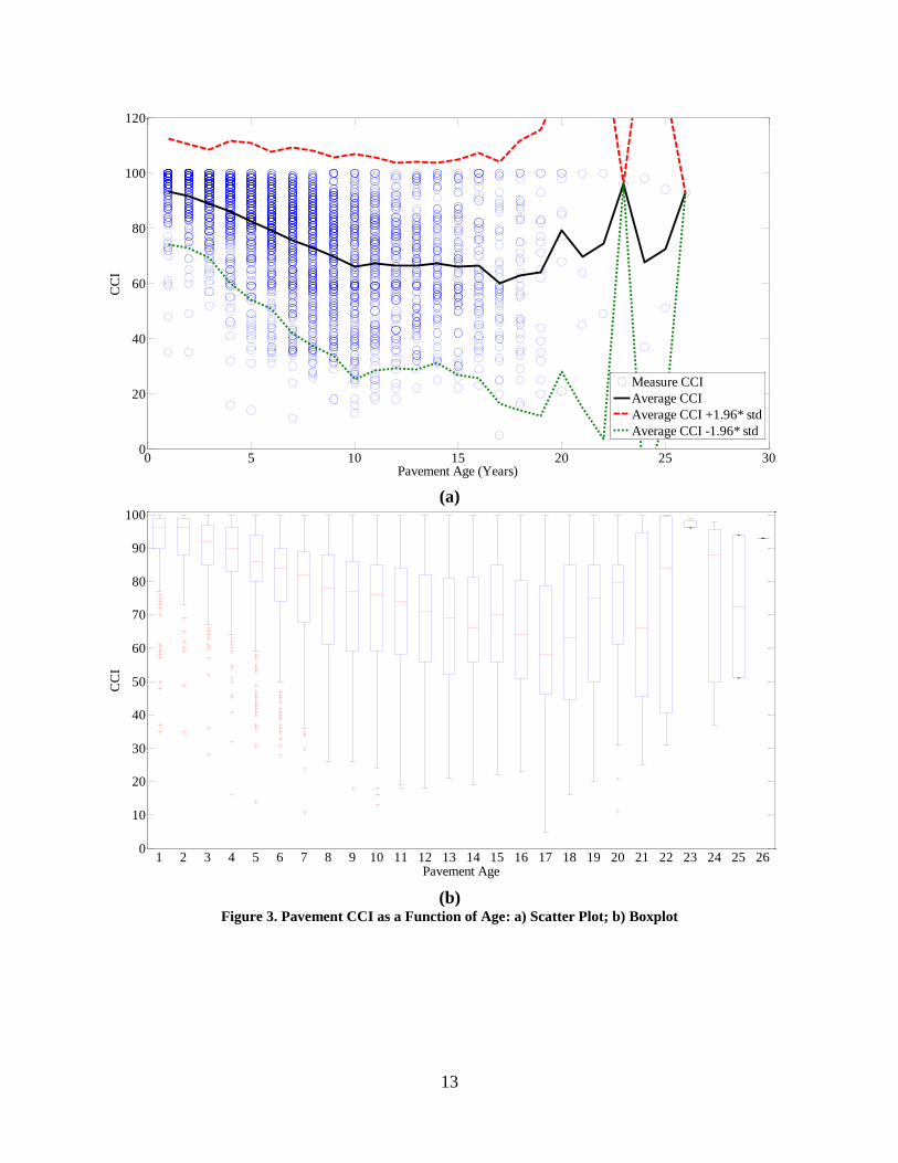
pavement sections had MSI values lower than one. Figure 3a shows the CCI values as a function

of pavement age. The mean of each age group with the two standard deviation range are also

shown in the figure. Clearly, the two standard deviation range (which is used to approximate the

95% confidence interval of normally distributed data) does not give an adequate representation

of the data as it extends beyond the CCI limit of 100. Figure 3b shows a box and whisker plot

with the box representing the data between the 25th and 75th percentile and the whiskers

extending to a maximum of 1.5 times the box range. Data points that fall outside the maximum

whiskers range are labeled with a “+” symbol.

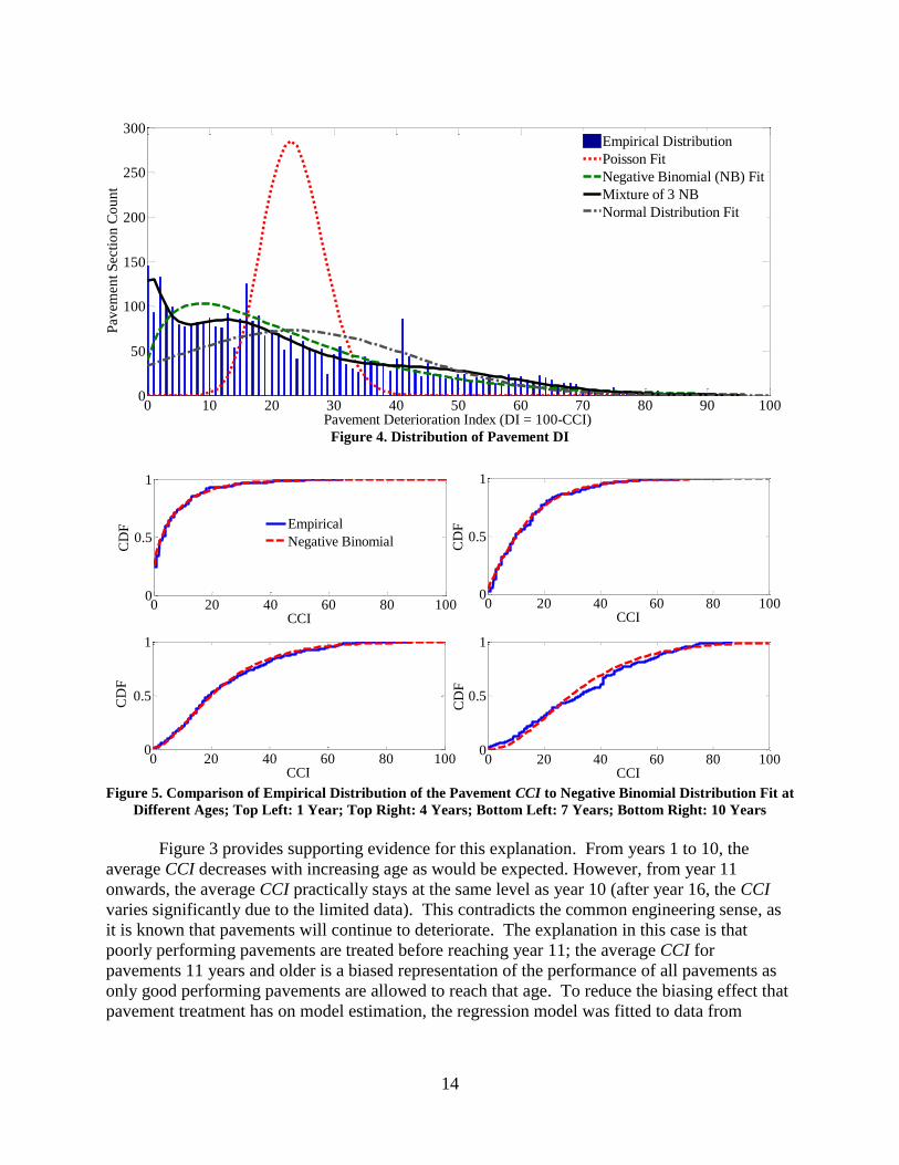
Figure 4 shows the distribution of the DI for all the data with different fitted theoretical

distributions; mainly, a Poisson distribution, a Normal distribution, a Negative Binomial

distribution, and a mixture of three Negative Binomial distributions. The Poisson distribution is

a discrete probability distribution for positive values and was considered because the DI values

are discrete and positive and combined with the Gamma distribution results in the Negative

Binomial distribution. The Poisson is restricted to having a variance equal to the mean of the

distribution, which results in a poor representation of the data. The Normal distribution allows

the variance to be independent of the mean and gives a better representation of the data;

however, it is not a discrete probability distribution, the fit is still not very good, and more

important, it allows for negative DI values, which is not realistic. The Negative Binomial

distribution gives a better fit to the data and is restricted to positive DI values.

Figure 5 shows the Negative Binomial Distribution fitted to DI observations obtained at a

fixed age (ages of 1, 4, 7, and 10 are shown). The fits for pavement ages 1, 4, and 7 years are

almost perfect. For the 10-year pavement age, the observed data deviate from the Negative

Binomial distribution, although it is still reasonable for modeling purposes (at least much more

reasonable than the Normal distribution assumption). There is, however, a very plausible

explanation for the lack of fit of the Negative Binomial distribution as the age increases. The

main purpose of a PMS is to keep the roads at an acceptable level of service. When a pavement

reaches an unacceptable condition level, action is taken to bring the condition back to acceptable

levels. This type of action biases the data, as only pavements that perform well are allowed to

reach a higher age. This means that if the condition of pavement sections at a given year, say 15

11

years, follows a certain distribution (in this case the Negative Binomial distribution), the

observed data will deviate from that distribution because the poorly performing pavements will

not be observed at 15 years because they would have already been treated.

Figure 1. Distribution of Pavement Section Ages; the age is determined from the last recorded pavement

treatment: a) Histogram; b) Cumulative Distribution

(a)

(b)

0 5 10 15 20 25 300

50

100

150

200

250

300

350

Pavement Section Age (Years)

Pav

emen

t S

ecti

on

Co

un

t

0 5 10 15 20 25 300

0.1

0.2

0.3

0.4

0.5

0.6

0.7

0.8

0.9

1

Pavement Section Age (Years)

Cu

mu

lati

ve

Dis

trib

uti

on

12

Figure 2. Distribution of MSI Values: a) Histogram; b) Cumulative Distribution

(a)

(b)

0 0.5 1 1.5 2 2.5 3 3.5 4 4.50

50

100

150

200

250

MSI

Pav

emen

t S

ecti

on

s C

ou

nt

0 0.5 1 1.5 2 2.5 3 3.5 4 4.50

0.1

0.2

0.3

0.4

0.5

0.6

0.7

0.8

0.9

1

MSI

Cu

mu

lati

ve

Dis

trib

uti

on

13

Figure 3. Pavement CCI as a Function of Age: a) Scatter Plot; b) Boxplot

(a)

(b)

0 5 10 15 20 25 300

20

40

60

80

100

120

Pavement Age (Years)

CC

I

Measure CCI

Average CCI

Average CCI +1.96* std

Average CCI -1.96* std

0

10

20

30

40

50

60

70

80

90

100

1 2 3 4 5 6 7 8 9 10 11 12 13 14 15 16 17 18 19 20 21 22 23 24 25 26Pavement Age

CC

I

14

Figure 4. Distribution of Pavement DI

Figure 5. Comparison of Empirical Distribution of the Pavement CCI to Negative Binomial Distribution Fit at

Different Ages; Top Left: 1 Year; Top Right: 4 Years; Bottom Left: 7 Years; Bottom Right: 10 Years

Figure 3 provides supporting evidence for this explanation. From years 1 to 10, the

average CCI decreases with increasing age as would be expected. However, from year 11

onwards, the average CCI practically stays at the same level as year 10 (after year 16, the CCI

varies significantly due to the limited data). This contradicts the common engineering sense, as

it is known that pavements will continue to deteriorate. The explanation in this case is that

poorly performing pavements are treated before reaching year 11; the average CCI for

pavements 11 years and older is a biased representation of the performance of all pavements as

only good performing pavements are allowed to reach that age. To reduce the biasing effect that

pavement treatment has on model estimation, the regression model was fitted to data from

0 10 20 30 40 50 60 70 80 90 1000

50

100

150

200

250

300

Pavement Deterioration Index (DI = 100-CCI)

Pav

emen

t S

ecti

on

Co

un

t

Empirical Distribution

Poisson Fit

Negative Binomial (NB) Fit

Mixture of 3 NB

Normal Distribution Fit

0 20 40 60 80 1000

0.5

1

CCI

CD

F

0 20 40 60 80 1000

0.5

1

CCI

CD

F

0 20 40 60 80 1000

0.5

1

CCI

CD

F

0 20 40 60 80 1000

0.5

1

CCI

CD

F

Empirical

Negative Binomial

15

observations of pavement sections that had the last treatment performed less than 10 years prior

to the observation.

Step 2. Deterioration Model Development

The estimate of the parameters of the model (Equation 2) were β0 = 1.7027, β1 = 0.0490,

β2 = 0.0866, and β3 = 0.1595, as obtained from the weighted Negative Binomial regression with

the data limited from 1 to 10 years (representing 76% of all the data). The overdispersion

parameter was equal to 0.3135. The AIC weight, w, for the model with MSI and the model

without MSI was less than 210-5

indicating that the model with the MSI is at least 50,000 times

more likely to be closer to the true pavement deterioration than the model without the MSI.

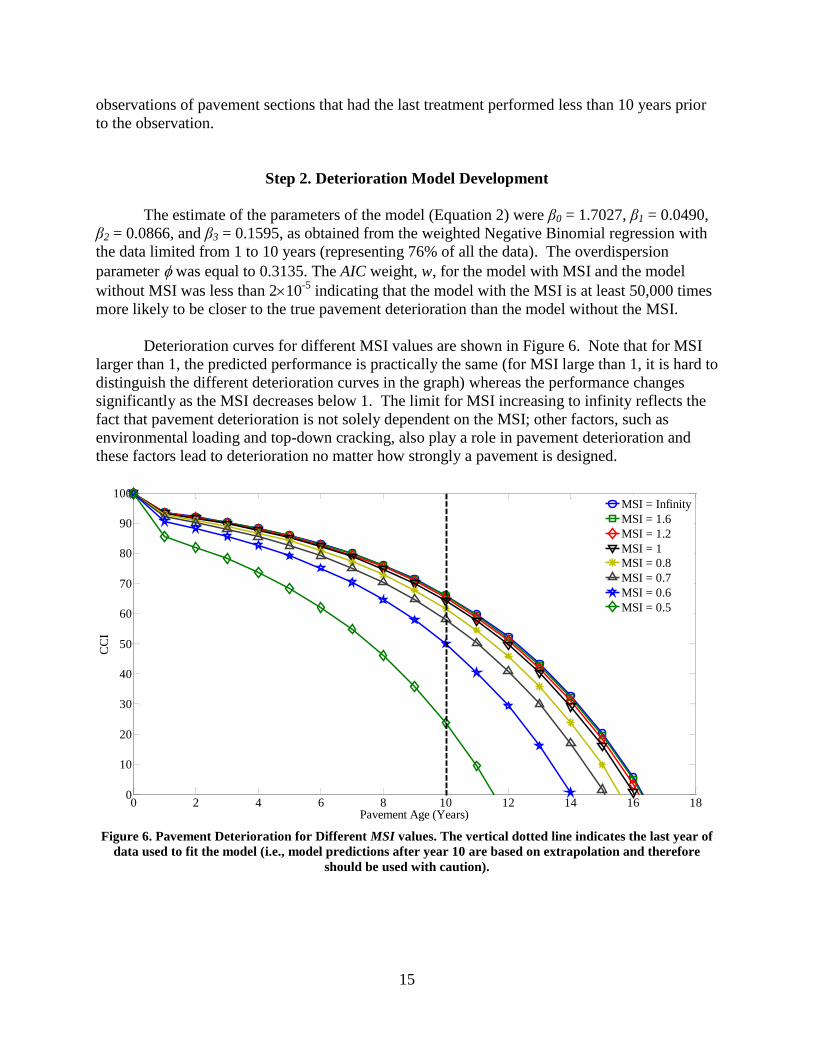
Deterioration curves for different MSI values are shown in Figure 6. Note that for MSI

larger than 1, the predicted performance is practically the same (for MSI large than 1, it is hard to

distinguish the different deterioration curves in the graph) whereas the performance changes

significantly as the MSI decreases below 1. The limit for MSI increasing to infinity reflects the

fact that pavement deterioration is not solely dependent on the MSI; other factors, such as

environmental loading and top-down cracking, also play a role in pavement deterioration and

these factors lead to deterioration no matter how strongly a pavement is designed.

Figure 6. Pavement Deterioration for Different MSI values. The vertical dotted line indicates the last year of

data used to fit the model (i.e., model predictions after year 10 are based on extrapolation and therefore

should be used with caution).

0 2 4 6 8 10 12 14 16 180

10

20

30

40

50

60

70

80

90

100


CC

I

MSI = Infinity

MSI = 1.6

MSI = 1.2

MSI = 1

MSI = 0.8

MSI = 0.7

MSI = 0.6

MSI = 0.5

16

Step 3. Empirical Bayes Estimate of Average Pavement Condition

The EB approach combines the model estimate with the individual observations of DI,

which does improve on the individual estimate of the pavement condition C. The EB estimated

condition takes into account the variability of the results of the pavement condition survey along

with the variability of the performance of individual pavement sections that is not taken into

account by the model to obtain a more accurate estimate of the pavement condition. The better

accuracy can be inferred from the fact that the EB estimate results in better prediction of future

pavement condition, which is presented at the end of this section.

EB Estimate of Pavement Condition Data

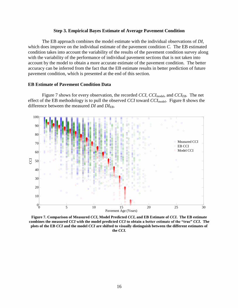
Figure 7 shows for every observation, the recorded CCI, CCImodel, and CCIEB. The net

effect of the EB methodology is to pull the observed CCI toward CCImodel. Figure 8 shows the

difference between the measured DI and DIEB.

Figure 7. Comparison of Measured CCI, Model Predicted CCI, and EB Estimate of CCI. The EB estimate

combines the measured CCI with the model predicted CCI to obtain a better estimate of the “true” CCI. The

plots of the EB CCI and the model CCI are shifted to visually distinguish between the different estimates of

the CCI.

0 5 10 15 20 25 300

10

20

30

40

50

60

70

80

90

100


CC

I

Measured CCI

EB CCI

Model CCI

17

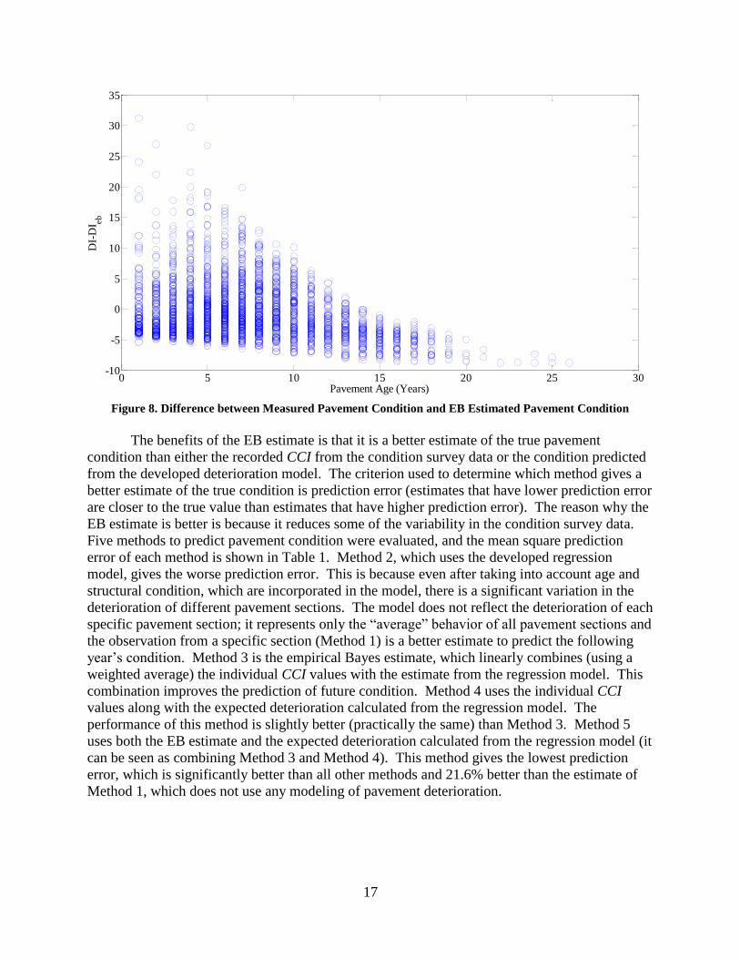
Figure 8. Difference between Measured Pavement Condition and EB Estimated Pavement Condition

The benefits of the EB estimate is that it is a better estimate of the true pavement

condition than either the recorded CCI from the condition survey data or the condition predicted

from the developed deterioration model. The criterion used to determine which method gives a

better estimate of the true condition is prediction error (estimates that have lower prediction error

are closer to the true value than estimates that have higher prediction error). The reason why the

EB estimate is better is because it reduces some of the variability in the condition survey data.

Five methods to predict pavement condition were evaluated, and the mean square prediction

error of each method is shown in Table 1. Method 2, which uses the developed regression

model, gives the worse prediction error. This is because even after taking into account age and

structural condition, which are incorporated in the model, there is a significant variation in the

deterioration of different pavement sections. The model does not reflect the deterioration of each

specific pavement section; it represents only the “average” behavior of all pavement sections and

the observation from a specific section (Method 1) is a better estimate to predict the following

year’s condition. Method 3 is the empirical Bayes estimate, which linearly combines (using a

weighted average) the individual CCI values with the estimate from the regression model. This

combination improves the prediction of future condition. Method 4 uses the individual CCI

values along with the expected deterioration calculated from the regression model. The

performance of this method is slightly better (practically the same) than Method 3. Method 5

uses both the EB estimate and the expected deterioration calculated from the regression model (it

can be seen as combining Method 3 and Method 4). This method gives the lowest prediction

error, which is significantly better than all other methods and 21.6% better than the estimate of

Method 1, which does not use any modeling of pavement deterioration.

0 5 10 15 20 25 30-10

-5

0

5

10

15

20

25

30

35


DI-

DI e

b

18

Table 1. Mean Square Error (MSE) of Prediction Using the Different Methods

to Estimate Future Pavement Condition

Method MSE Prediction MSE Ratio with Method 1

1 143.2 1.000

2 227.0 1.585

3 130.9 0.914

4 129.2 0.902

5 112.2 0.784

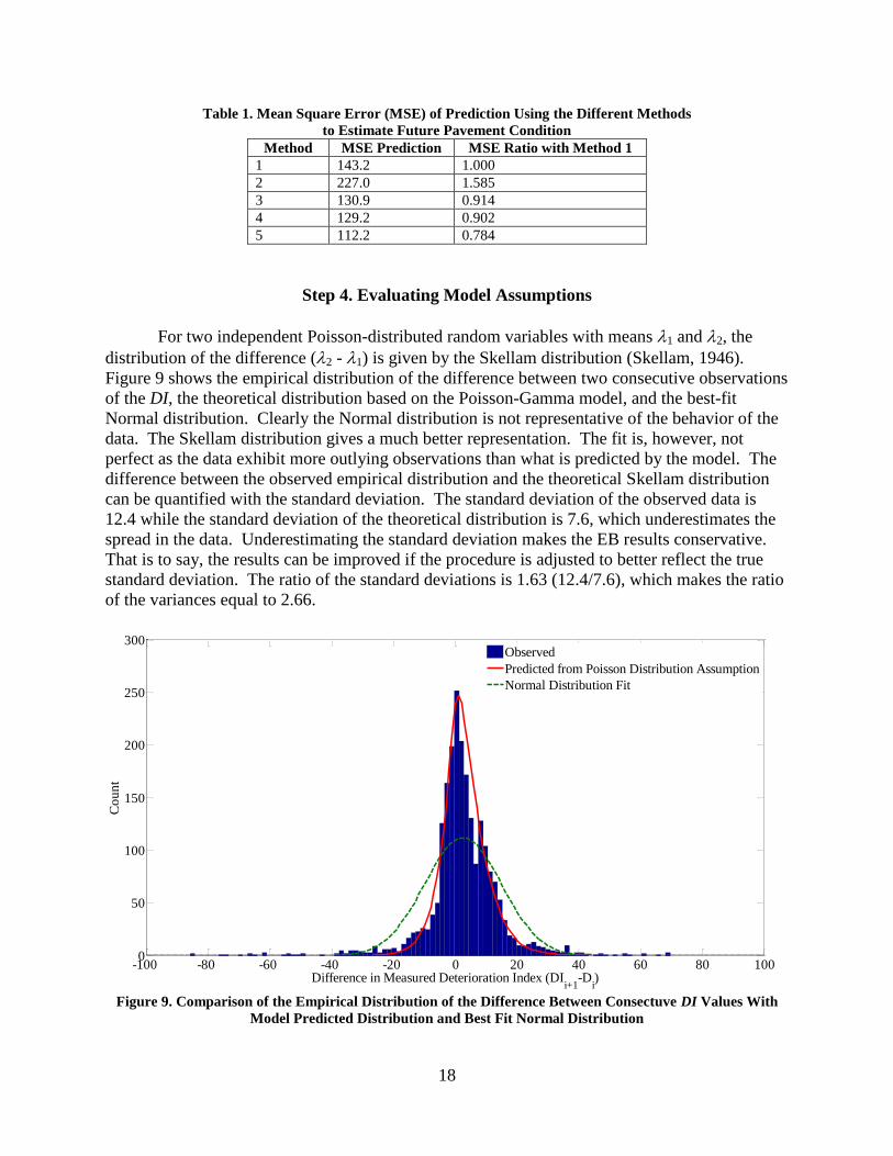
Step 4. Evaluating Model Assumptions

For two independent Poisson-distributed random variables with means 1 and 2, the

distribution of the difference (2 - 1) is given by the Skellam distribution (Skellam, 1946).

Figure 9 shows the empirical distribution of the difference between two consecutive observations

of the DI, the theoretical distribution based on the Poisson-Gamma model, and the best-fit

Normal distribution. Clearly the Normal distribution is not representative of the behavior of the

data. The Skellam distribution gives a much better representation. The fit is, however, not

perfect as the data exhibit more outlying observations than what is predicted by the model. The

difference between the observed empirical distribution and the theoretical Skellam distribution

can be quantified with the standard deviation. The standard deviation of the observed data is

12.4 while the standard deviation of the theoretical distribution is 7.6, which underestimates the

spread in the data. Underestimating the standard deviation makes the EB results conservative.

That is to say, the results can be improved if the procedure is adjusted to better reflect the true

standard deviation. The ratio of the standard deviations is 1.63 (12.4/7.6), which makes the ratio

of the variances equal to 2.66.

Figure 9. Comparison of the Empirical Distribution of the Difference Between Consectuve DI Values With

Model Predicted Distribution and Best Fit Normal Distribution

-100 -80 -60 -40 -20 0 20 40 60 80 1000

50

100

150

200

250

300

Difference in Measured Deterioration Index (DIi+1

-Di)

Co

un

t

Observed

Predicted from Poisson Distribution Assumption

Normal Distribution Fit

19

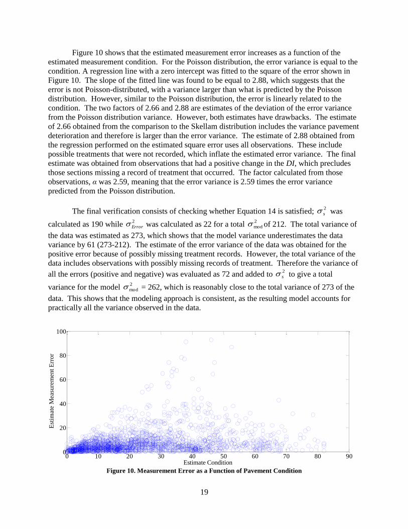
Figure 10 shows that the estimated measurement error increases as a function of the

estimated measurement condition. For the Poisson distribution, the error variance is equal to the

condition. A regression line with a zero intercept was fitted to the square of the error shown in

Figure 10. The slope of the fitted line was found to be equal to 2.88, which suggests that the

error is not Poisson-distributed, with a variance larger than what is predicted by the Poisson

distribution. However, similar to the Poisson distribution, the error is linearly related to the

condition. The two factors of 2.66 and 2.88 are estimates of the deviation of the error variance

from the Poisson distribution variance. However, both estimates have drawbacks. The estimate

of 2.66 obtained from the comparison to the Skellam distribution includes the variance pavement

deterioration and therefore is larger than the error variance. The estimate of 2.88 obtained from

the regression performed on the estimated square error uses all observations. These include

possible treatments that were not recorded, which inflate the estimated error variance. The final

estimate was obtained from observations that had a positive change in the DI, which precludes

those sections missing a record of treatment that occurred. The factor calculated from those

observations, α was 2.59, meaning that the error variance is 2.59 times the error variance

predicted from the Poisson distribution.

The final verification consists of checking whether Equation 14 is satisfied; was

calculated as 190 while was calculated as 22 for a total of 212. The total variance of

the data was estimated as 273, which shows that the model variance underestimates the data

variance by 61 (273-212). The estimate of the error variance of the data was obtained for the

positive error because of possibly missing treatment records. However, the total variance of the

data includes observations with possibly missing records of treatment. Therefore the variance of

all the errors (positive and negative) was evaluated as 72 and added to to give a total

variance for the model = 262, which is reasonably close to the total variance of 273 of the

data. This shows that the modeling approach is consistent, as the resulting model accounts for

practically all the variance observed in the data.

Figure 10. Measurement Error as a Function of Pavement Condition

2

s2

Error 2

mod

2

s2

mod

0 10 20 30 40 50 60 70 80 900

20

40

60

80

100

Estimate Condition

Est

imat

e M

easu

rem

ent

Err

or

20

CONCLUSIONS

The pavement structural condition (MSI parameter) is a significant parameter that affects the

pavement condition: using the AIC criterion, the model that incorporates the pavement

structural parameter as an explanatory variable of the pavement condition was more than

50,000 times more likely than the model that does not incorporate the pavement structural

condition.

The Negative Binomial distribution gives a good representation of the pavement condition:

this allows for a better understanding and modeling approach to pavement condition where

variability in pavement condition can be decomposed into variability due to different

performance of different pavement sections and variability due to error in measuring the

pavement condition. The resulting model can be used for network-level pavement

management.

Condition of pavement sections older than 10 years do not represent the typical (expected)

performance of pavement sections: pavement sections are rehabilitated once they reach an

unacceptable condition level. Most pavement sections need some sort of treatment before 11

years have passed since the last treatment and only pavement sections that perform well

reach 11 years of age or more. Therefore, those pavement sections give a biased

representation of pavement condition after 10 years.

The optimal estimate of the pavement condition is one that combines the observed condition

with the model predicted condition: the estimate is obtained by an EB approach, which

combines the model estimate with the observed condition through a weighted average. The

weight is determined by the relative variability of the error in the measurement of the

pavement condition and the variability of the performance of different pavement conditions.

The model on its own gives an inaccurate estimate of the pavement condition with a mean

square error that is about 1.58 times the mean square error prediction of future observations.

However, combining the observations with the model resulted in an estimated mean square

error prediction that is about 0.78 times the mean square error prediction of the observations.

The estimate of the improvement is based on cross-validation where observations are held

out and used to estimate the mean square error prediction.

RECOMMENDATIONS

1. VDOT’s Maintenance Division should implement the empirical Bayes method to determine

the pavement condition of Interstate roads: the EB method was found to improve the

prediction of future CCI measurements by an estimated average of 21.6%.

2. VDOT’s Maintenance Division should develop a similar approach for the pavement

condition of primary and high-volume secondary roads: the implementation for secondary

roads that are only evaluated at 5-year cycles is especially needed, and for this purpose FWD

data collection at the network level is suggested for these roads. The EB method combined

21

with the modeled deterioration should provide for a better prediction of the conditions of

secondary roads during the years when the condition is not collected.

3. VDOT’s Maintenance Division should continue performing network-level pavement

structural evaluation: The pavement structural condition summarized in terms of the MSI

was found to affect the rate of pavement deterioration.

BENEFITS AND IMPLEMENTATION

Benefits

The primary benefit of this study to VDOT is that VDOT will be able to predict more

accurately the future condition of pavement sections on its network using the empirical Bayes

approach. Although no direct cost savings are anticipated, improved predictions should support

more efficient use of resources through VDOT’s needs-based budgeting process.

The empirical Bayes (EB) approach can further improve the estimate of the pavement

condition. The proposed approach can improve the mean square error prediction of the future

(next year’s) pavement condition by 21.6%. This improved estimate of the future pavement

condition is expected to minimize the difference between network-level planning and project-

level treatment selection, which will result in more effective management of the pavement assets.

Implementation

With regard to Recommendations 1 and 2, VDOT’s Maintenance Division will work in

cooperation with VDOT’s Information Technology Division to implement the suggested

methodology within the PMS and apply these steps wherever recent and reasonable data are

available. It is expected that this will have an impact on the results of the network level analysis;

maintenance and rehabilitation recommendations from the PMS; and budgetary needs and other

reports currently prepared by VDOT. VDOT’s Maintenance Division should further perform

sensitivity analyses on the final results and recommend changes to the current methodologies and

allocation wherever applicable.

With regard to Recommendation 3, VDOT plans to continue collecting network level

structural condition data. VDOT is a participating agency in Transportation Pooled Fund Study

TPF-5(282), Demonstration of Network Level Pavement Structural Evaluation with Traffic

Speed Deflectometer. This pooled fund study is anticipated to be complete by the end of the

fourth quarter of calendar year 2016 and will provide suggestions to VDOT as to how best to

accomplish this testing.

22

ACKNOWLEDGMENTS

The authors acknowledge the contributions of the project’s technical review panel:

Tanveer Chowdhury, David Shiells, and Bryan Smith. The authors also thank Raja Shekharan

and Akyiaa Morrison from VDOT for their review of, and input to, the project report.

REFERENCES

Bryce, J.M., Flintsch, G.W., Katicha, S.W., and Diefenderfer, B.K. (2013). Developing a

Network-Level Structural Capacity Index for Structural Evaluation of Pavements.

VCTIR 13-R9. Virginia Center for Transportation Innovation and Research,

Charlottesville.

Burnham, K.P., and Anderson, D.R. (2004). Multimodal Inference: Understanding AIC and

BIC in Model Selection. Sociological Methods and Research, Vol. 33, No. 2, pp. 261–

304.

Efron, B., and Morris, C. (1973). Stein’s Estimation Rule and Its Competitors: An Empirical

Bayes Approach. Journal of the American Statistical Association, Vol. 63, No. 341, pp.

117–130.

Flora, W. (2009). Development of a Structural Index for Pavement Management: An

Exploratory Analysis. Master’s Thesis, Purdue University, West Lafayette, IN.

Hartigan, J.A. (1969). Linear Bayesian Methods. Journal of the Royal Statistical Society:

Series B (Methodological), Vol. 31, No. 3, pp. 446-454.

Skellam, J.G. (1946). The Frequency Distribution of the Difference Between Two Poisson

Variates Belonging to Different Populations. Journal of the Royal Statistical Society,

Vol. 109, No.3, pp. 296.

Stantec. (2007). Development of Performance Models for Virginia Department of

Transportation Pavement Management System. Virginia Department of Transportation,

Richmond.

Zaghloul, S., He, Z., Vitillo, N., and Kerr, B. (1998). Project Scoping Using Falling Weight

Deflectometer Testing: New Jersey Experience. In Transportation Research Record:

Journal of the Transportation Research Board, No. 1643. Transportation Research

Board of the National Academies, Washington, DC, pp. 34-43.

23

APPENDIX A

MODIFIED STRUCTURAL INDEX METHODOLOGY

This appendix presents the methodology to calculate the modified structural index (MSI)

from FWD data and describes how to update the MSI based on applied pavement treatment.

Calculating the Modified Structural Capacity Index (MSI)

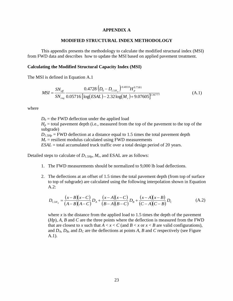
The MSI is defined in Equation A.1

36777.2

7581.04810.0

5.10

07605.9log32.2log05716.0

4728.0

r

pH

req

eff

MESAL

HDD

SN

SNMSI

p (A.1)

where

D0 = the FWD deflection under the applied load

Hp = total pavement depth (i.e., measured from the top of the pavement to the top of the

subgrade)

D1.5Hp = FWD deflection at a distance equal to 1.5 times the total pavement depth

Mr = resilient modulus calculated using FWD measurements

ESAL = total accumulated truck traffic over a total design period of 20 years.

Detailed steps to calculate of D1.5Hp, Mr, and ESAL are as follows:

1. The FWD measurements should be normalized to 9,000 lb load deflections.

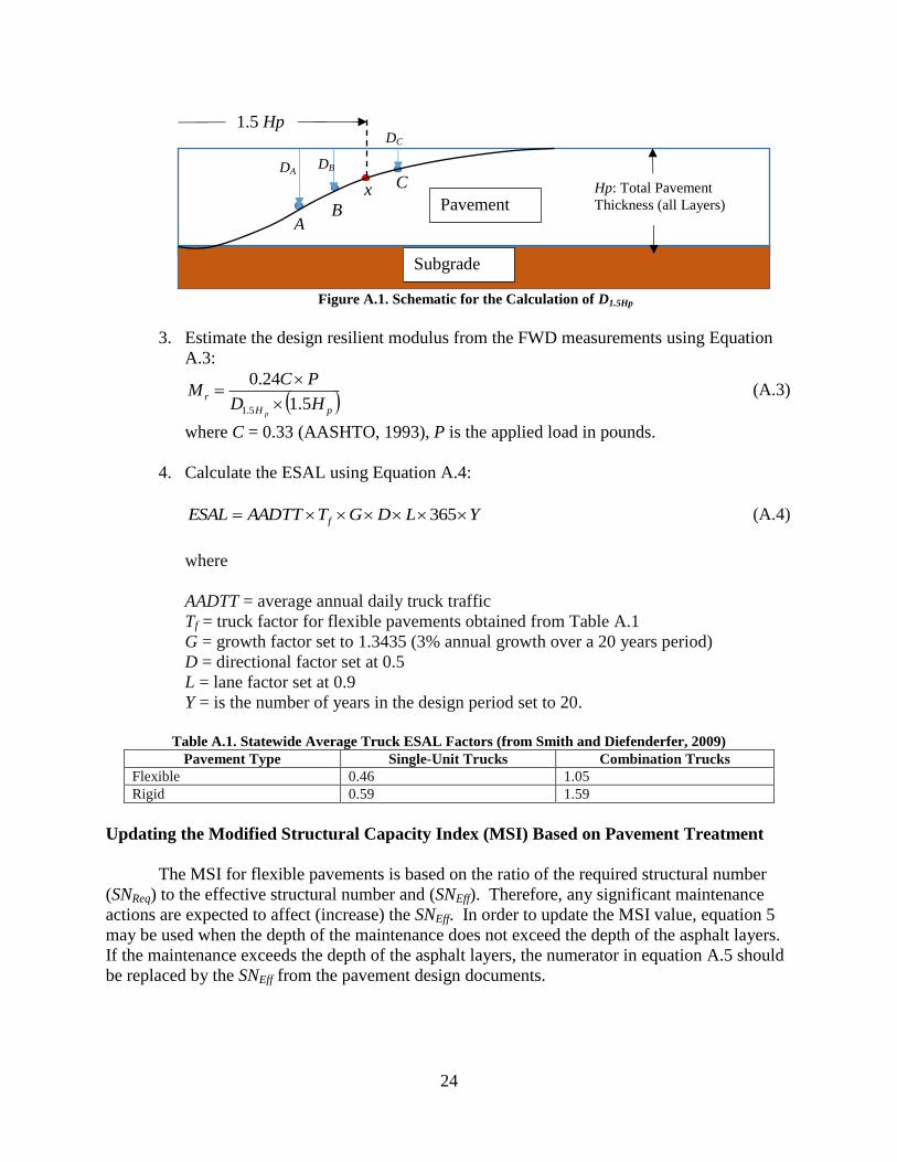
2. The deflections at an offset of 1.5 times the total pavement depth (from top of surface

to top of subgrade) are calculated using the following interpolation shown in Equation

A.2:

CBAH D

BCAC

BxAxD

CBAB

CxAxD

CABA

CxBxD

p

5.1

(A.2)

where x is the distance from the applied load to 1.5 times the depth of the pavement

(Hp), A, B and C are the three points where the deflection is measured from the FWD

that are closest to x such that A < x < C (and B < x or x < B are valid configurations),

and DA, DB, and DC are the deflections at points A, B and C respectively (see Figure

A.1).

24

Figure A.1. Schematic for the Calculation of D1.5Hp

3. Estimate the design resilient modulus from the FWD measurements using Equation

A.3:

pH

rHD

PCM

p5.1

24.0

5.1

(A.3)

where C = 0.33 (AASHTO, 1993), P is the applied load in pounds.

4. Calculate the ESAL using Equation A.4:

YLDGTAADTTESAL f 365 (A.4)

where

AADTT = average annual daily truck traffic

Tf = truck factor for flexible pavements obtained from Table A.1

G = growth factor set to 1.3435 (3% annual growth over a 20 years period)

D = directional factor set at 0.5

L = lane factor set at 0.9

Y = is the number of years in the design period set to 20.

Table A.1. Statewide Average Truck ESAL Factors (from Smith and Diefenderfer, 2009)

Pavement Type Single-Unit Trucks Combination Trucks

Flexible 0.46 1.05

Rigid 0.59 1.59

Updating the Modified Structural Capacity Index (MSI) Based on Pavement Treatment

The MSI for flexible pavements is based on the ratio of the required structural number

(SNReq) to the effective structural number and (SNEff). Therefore, any significant maintenance

actions are expected to affect (increase) the SNEff. In order to update the MSI value, equation 5

may be used when the depth of the maintenance does not exceed the depth of the asphalt layers.

If the maintenance exceeds the depth of the asphalt layers, the numerator in equation A.5 should

be replaced by the SNEff from the pavement design documents.

Subgrade

Pavement A

C

B

x

DA

Hp: Total Pavement

Thickness (all Layers)

1.5 Hp

DB

DC

25

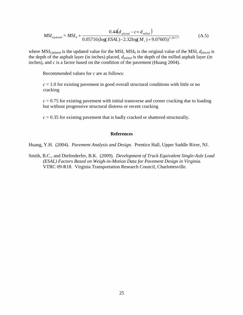
2.367770

9.07605))2.32log(-)(log(0.05716

44.0=

r

milledplaced

UpdatedMESAL

dcdMSIMSI (A.5)

where MSIUpdated is the updated value for the MSI, MSI0 is the original value of the MSI, dplaced is

the depth of the asphalt layer (in inches) placed, dmilled is the depth of the milled asphalt layer (in

inches), and c is a factor based on the condition of the pavement (Huang 2004).

Recommended values for c are as follows:

c = 1.0 for existing pavement in good overall structural conditions with little or no

cracking

c = 0.75 for existing pavement with initial transverse and corner cracking due to loading

but without progressive structural distress or recent cracking

c = 0.35 for existing pavement that is badly cracked or shattered structurally.

References

Huang, Y.H. (2004). Pavement Analysis and Design. Prentice Hall, Upper Saddle River, NJ.

Smith, B.C., and Diefenderfer, B.K. (2009). Development of Truck Equivalent Single-Axle Load

(ESAL) Factors Based on Weigh-in-Motion Data for Pavement Design in Virginia.

VTRC 09-R18. Virginia Transportation Research Council, Charlottesville.

26

27

APPENDIX B

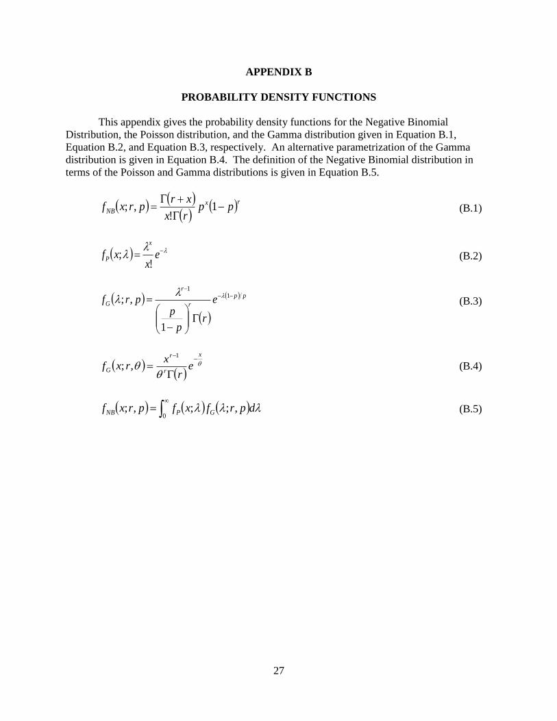
PROBABILITY DENSITY FUNCTIONS

This appendix gives the probability density functions for the Negative Binomial

Distribution, the Poisson distribution, and the Gamma distribution given in Equation B.1,

Equation B.2, and Equation B.3, respectively. An alternative parametrization of the Gamma

distribution is given in Equation B.4. The definition of the Negative Binomial distribution in

terms of the Poisson and Gamma distributions is given in Equation B.5.

rx

NB pprx

xrprxf

1

!,; (B.1)

e

xxf

x

P!

; (B.2)

pp

r

r

G e

rp

pprf

11

1

,; (B.3)

x

r

r

G er

xrxf

1

,; (B.4)

0

,;;,; dprfxfprxf GPNB (B.5)

28

29

APPENDIX C

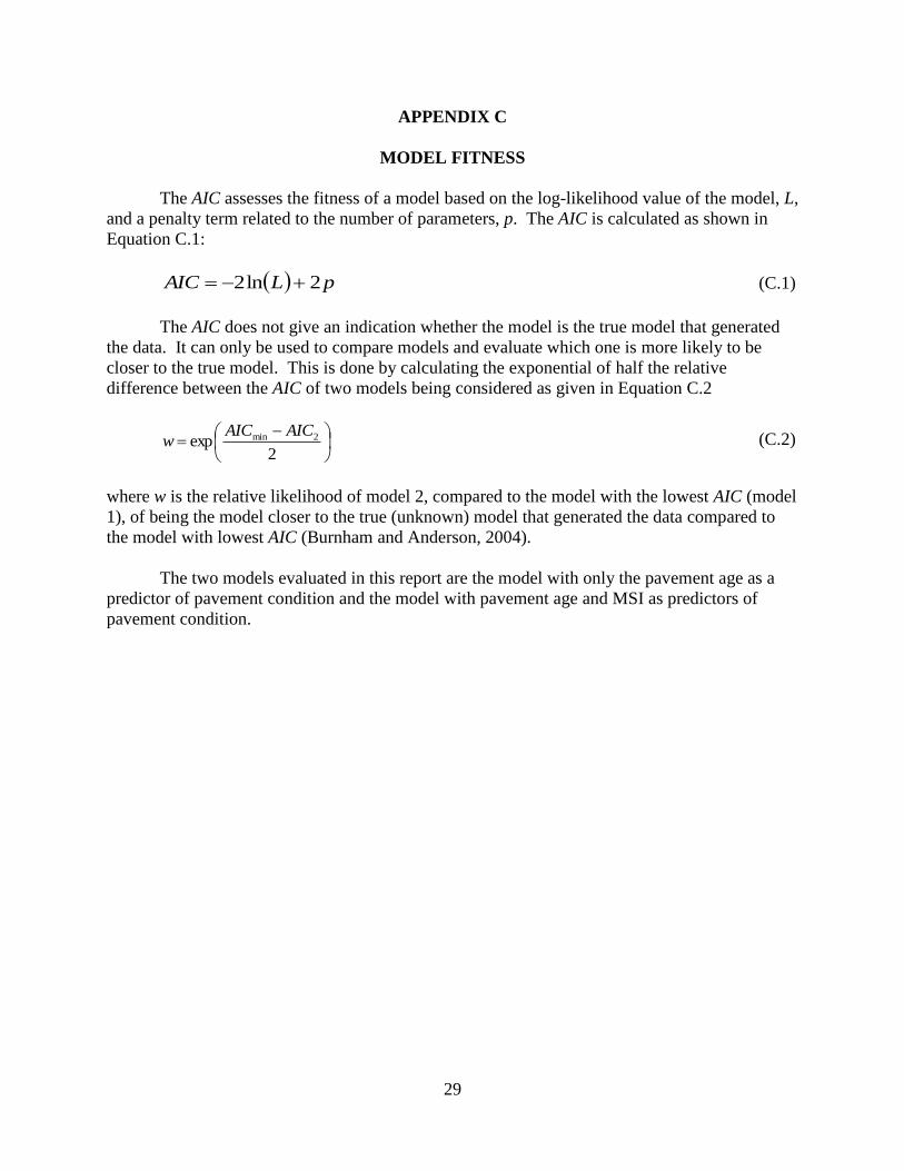
MODEL FITNESS

The AIC assesses the fitness of a model based on the log-likelihood value of the model, L,

and a penalty term related to the number of parameters, p. The AIC is calculated as shown in

Equation C.1:

pLAIC 2ln2 (C.1)

The AIC does not give an indication whether the model is the true model that generated

the data. It can only be used to compare models and evaluate which one is more likely to be

closer to the true model. This is done by calculating the exponential of half the relative

difference between the AIC of two models being considered as given in Equation C.2

2exp 2min AICAIC

w (C.2)

where w is the relative likelihood of model 2, compared to the model with the lowest AIC (model

1), of being the model closer to the true (unknown) model that generated the data compared to

the model with lowest AIC (Burnham and Anderson, 2004).

The two models evaluated in this report are the model with only the pavement age as a

predictor of pavement condition and the model with pavement age and MSI as predictors of

pavement condition.

30

31

APPENDIX D

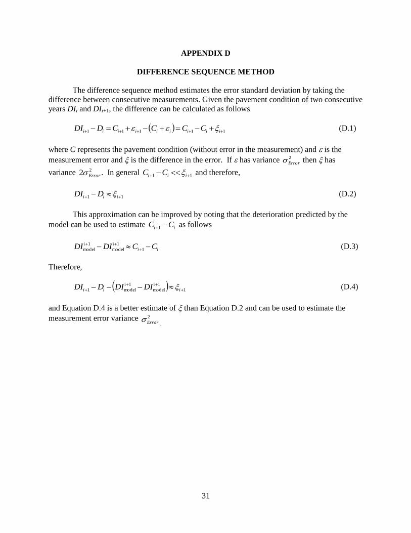
DIFFERENCE SEQUENCE METHOD

The difference sequence method estimates the error standard deviation by taking the

difference between consecutive measurements. Given the pavement condition of two consecutive

years DIi and DIi+1, the difference can be calculated as follows

11111 iiiiiiiii CCCCDDI (D.1)

where C represents the pavement condition (without error in the measurement) and is the

measurement error and is the difference in the error. If has variance 2

Error then has

variance 22 Error . In general 11 iii CC and therefore,

11 iii DDI (D.2)

This approximation can be improved by noting that the deterioration predicted by the

model can be used to estimate ii CC 1 as follows

ii CCDIDI

1

1i

model

1i

model (D.3)

Therefore,

1

1i

model

1i

model1

iii DIDIDDI (D.4)

and Equation D.4 is a better estimate of than Equation D.2 and can be used to estimate the

measurement error variance 2

Error.

32

33

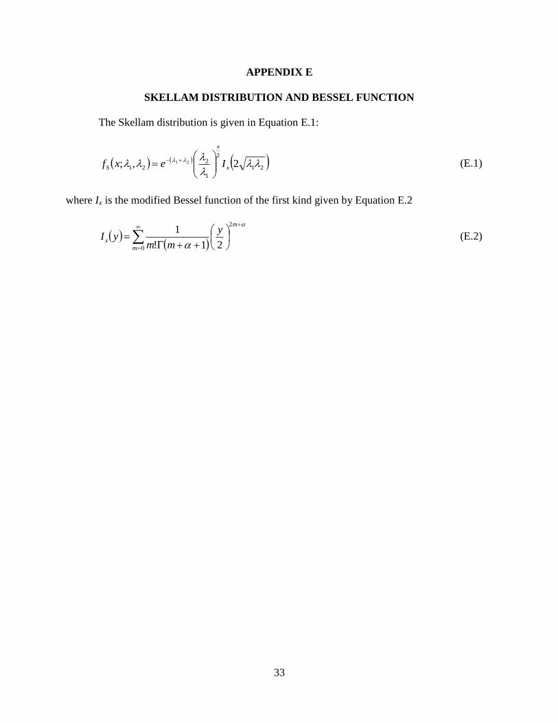
APPENDIX E

SKELLAM DISTRIBUTION AND BESSEL FUNCTION

The Skellam distribution is given in Equation E.1:

21

2

1

221 2,; 21

x

x

S Iexf

(E.1)

where Ix is the modified Bessel function of the first kind given by Equation E.2

0

2

21!

1

m

m

x

y

mmyI

(E.2)

34

35

APPENDIX F

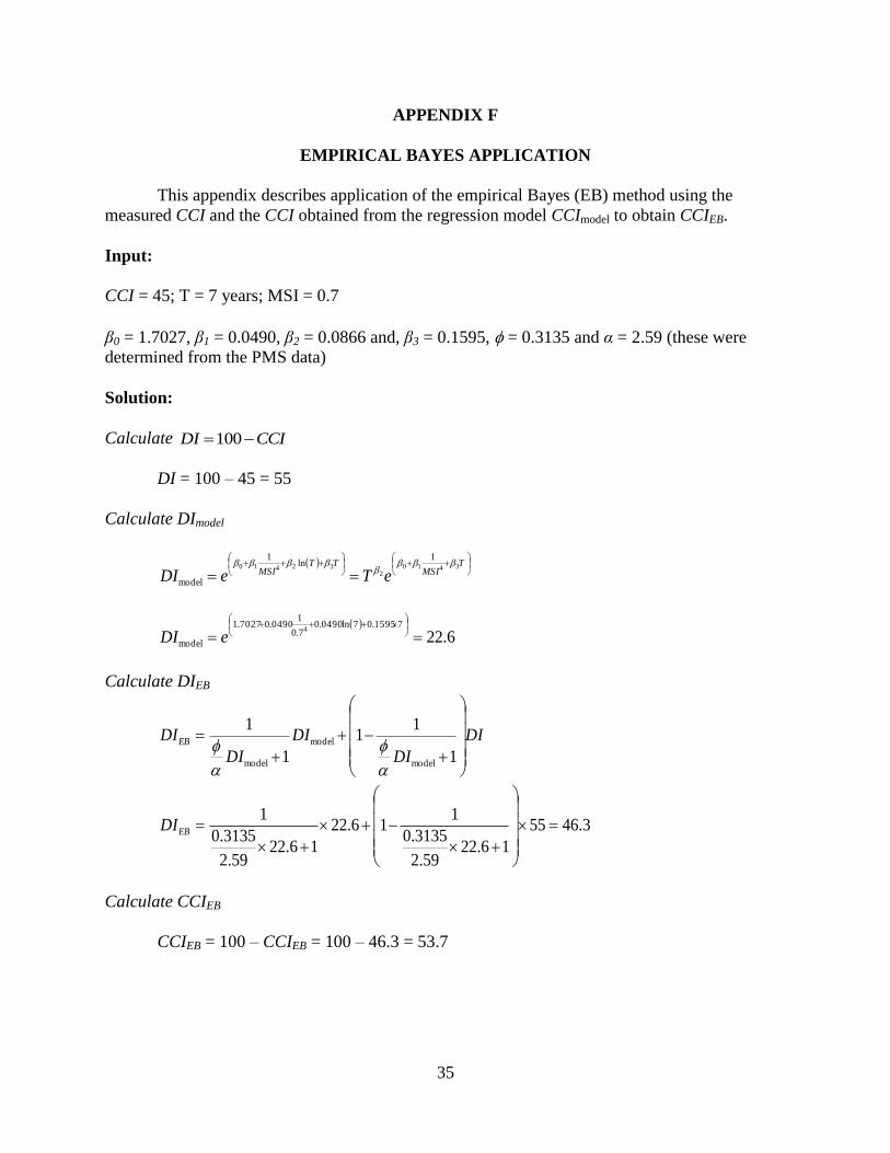
EMPIRICAL BAYES APPLICATION

This appendix describes application of the empirical Bayes (EB) method using the

measured CCI and the CCI obtained from the regression model CCImodel to obtain CCIEB.

Input:

CCI = 45; T = 7 years; MSI = 0.7

β0 = 1.7027, β1 = 0.0490, β2 = 0.0866 and, β3 = 0.1595, = 0.3135 and α = 2.59 (these were

determined from the PMS data)

Solution:

Calculate CCIDI 100

DI = 100 – 45 = 55

Calculate DImodel

T

MSITT

MSI eTeDI3410

232410

1ln

1

model

6.2271595.07ln0490.0

7.0

10490.07027.1

model

4

eDI

Calculate DIEB

DI

DI

DI

DI

DIEB

1

11

1

1

model

model

model

3.4655

16.2259.2

3135.0

116.22

16.2259.2

3135.0

1

EBDI

Calculate CCIEB

CCIEB = 100 – CCIEB = 100 – 46.3 = 53.7

Documents

Development of Enhanced Pavement Deterioration Curves · amec foster wheeler ... development of enhanced pavement deterioration curves ... development of enhanced pavement deterioration