Embed Size (px)
Citation preview

DEVELOPMENT OF DESIGN TOOL FOR STATICALLY
EQUIVALENT DEEPWATER MOORING SYSTEMS
A Thesis
by
IKPOTO ENEFIOK UDOH
Submitted to the Office of Graduate Studies of Texas A&M University
in partial fulfillment of the requirements for the degree of
MASTER OF SCIENCE
December 2008
Major Subject: Ocean Engineering

DEVELOPMENT OF DESIGN TOOL FOR STATICALLY
EQUIVALENT DEEPWATER MOORING SYSTEMS
A Thesis
by
IKPOTO ENEFIOK UDOH
Submitted to the Office of Graduate Studies of Texas A&M University
in partial fulfillment of the requirements for the degree of
MASTER OF SCIENCE
Approved by:
Chair of Committee, Richard Mercier Committee Members, Harry Jones Jerome Schubert Head of Department, David V. Rosowsky
December 2008
Major Subject: Ocean Engineering

iii
ABSTRACT
Development of Design Tool for Statically Equivalent Deepwater Mooring
Systems. (December 2008)
Ikpoto Enefiok Udoh, B. Eng., University of Port Harcourt, Nigeria
Chair of Advisory Committee: Dr. Richard Mercier
Verifying the design of floating structures adequately requires both numerical
simulations and model testing, a combination of which is referred to as the
hybrid method of design verification. The challenge in direct scaling of moorings
for model tests is the depth and spatial limitations in wave basins. It is therefore
important to design and build equivalent mooring systems to ensure that the
static properties (global restoring forces and global stiffness) of the prototype
floater are matched by those of the model in the wave basin prior to testing.
A fit-for-purpose numerical tool called STAMOORSYS is developed in this
research for the design of statically equivalent deepwater mooring systems. The
elastic catenary equations are derived and applied with efficient algorithm to
obtain local and global static equilibrium solutions. A unique design page in
STAMOORSYS is used to manually optimize the system properties in search of
a match in global restoring forces and global stiffness. Up to eight mooring lines
can be used in analyses and all lines have the same properties. STAMOORSYS
is validated for single-line mooring analysis using LINANL and Orcaflex, and for
global mooring analysis using MOORANL and Orcaflex. A statically equivalent
deepwater mooring system for a representative structure that could be tested in
the Offshore Technology Research Center at Texas A&M University is then
designed using STAMOORSYS and the results are discussed.

iv
DEDICATION
This work is dedicated to the almighty God for his kindness and mercies.

v
ACKNOWLEDGEMENTS
The successful completion of my thesis was possible thanks to the support of
many people, including my committee members, professors, friends and family. I
give my sincere thanks to my committee chair, Dr. Richard Mercier, for the
opportunity to be a part of this research and for inspiring me to work hard at it.
His insistence on top quality work drove my ability to search deep for adequate
solutions to research challenges. I appreciate Dr. Harry Jones for his support,
guidance, and timely feedback during my research. I thank Dr. Jerome Schubert
for honest feedback on my work and for serving effectively on my committee
even under short notice. I thank Dr. Robert Randall for his guidance and
counseling which helped me set a balance between research and other aspects
of my academic pursuits. My thanks also go to Dr. Scott Socolofsky for his ideas
which inspired me to explore possible routes in search of the best approaches to
overcome some of my research challenges.
I thank my parents Hon. Justice and Barr. (Lady) Enefiok Udoh, for their
immeasurable support during the entire course of my studies. I extend my
gratitude to my love Agnes Iyoho, who encouraged me and stood by me through
it all. I appreciate my brother Anyanya and my sisters Uduak and Ndifreke for
their moral support and guidance whenever I needed to make difficult decisions.
I acknowledge my friends James Ofoegbu, Amir Izadparast, Suresh Rajendran,
Adeniyi Olumide and Akan Ndey for making themselves available anytime it was
necessary to have fun and ease the troubled research mind. Their pieces of
advice and jokes made a world of difference in re-generating the strength and
motivation to accomplish the goals of my research.

vi
TABLE OF CONTENTS
Page
ABSTRACT ................................................................................................. iii
DEDICATION .............................................................................................. iv
ACKNOWLEDGEMENTS ............................................................................ v
TABLE OF CONTENTS .............................................................................. vi
LIST OF FIGURES ..................................................................................... viii
LIST OF TABLES ........................................................................................ xiii
CHAPTER
I INTRODUCTION: MOORING OF OFFSHORE STRUCTURES 1
1.1 Introduction .................................................................................... 1 1.2 Objective of research ..................................................................... 3 1.3 Truncated versus equivalent mooring systems .............................. 5 1.4 Scope of research project ............................................................. 23 1.5 Mooring lines and components of mooring systems .......................................................................................... 24 1.6 Offshore mooring systems ............................................................. 33
II DESIGN-RELATED LIMITATIONS OF EXISTING
MOORING METHODOLOGIES .......................................................... 36
2.1 Challenges in deepwater model testing using equivalent mooring systems ......................................................... 36 2.2 Suitability of existing approaches for mooring line analysis .................................................................... 47

vii
CHAPTER Page
2.3 Engineering behavior and modes of failure of mooring lines .................................................................................. 61
III FORMULATION OF STAMOORSYS ............................................... 70
3.1 General principles in static analysis of spread catenary mooring systems ........................................................... 71 3.2 Algorithm used in STAMOORSYS for the design of statically equivalent spread mooring systems ............................. 84 3.3 A description of the features in STAMOORSYS ......................... 99
IV APPLICATION OF STAMOORSYS IN DESIGN OF
STATICALLY EQUIVALENT MOORING SYSTEMS ...................... 109
4.1 Analysis of single line mooring systems using STAMOORSYS, Orcaflex and LINANL ....................................... 109 4.2 Validation of STAMOORSYS for static global analysis
of spread mooring systems ......................................................... 124 4.3 Design of statically equivalent deepwater mooring
system ........................................................................................ 130
V SUMMARY AND CONCLUSIONS 140
5.1 Economic advantages of STAMOORSYS ................................. 141 5.2 Limitations of STAMOORSYS and up-coming modifications ............................................................................... 142 5.3 Conclusions ............................................................................... 144
REFERENCES ........................................................................................ 146
APPENDIX A ........................................................................................... 149
APPENDIX B ........................................................................................... 152
VITA ......................................................................................................... 156

viii
LIST OF FIGURES
FIGURE Page
1.1 Sketch of truncated and full depth mooring systems ......................... 6
1.2 The hybrid approach to design verification ........................................ 10
1.3 Discrepancies between full depth floater and model scale floater ................................................................................................ 13
1.4 Sketch of discrepancies between full depth and model scale systems ............................................................................................. 13
1.5 Dependence of uncertainties on model scale ................................... 17
1.6 Model tank station-keeping equipment ............................................. 20
1.7 Static mooring line responses – prototype versus model ................. 21
1.8 A sketch showing the use of point masses in truncated systems .... 22
1.9 Stainless steel cable ......................................................................... 25
1.10 (a) Very flexible steel cable (b) Flexible steel cable ........................ 26
1.11 Studless mooring chain .................................................................... 27
1.12 Stud-linked mooring chain ................................................................ 27
1.13 Synthetic fiber rope .......................................................................... 28
1.14 Anchor set-up for basin scale mooring ............................................ 30
1.15 Clamping device for basin scale mooring line ................................. 30
1.16 Connectors for model scale mooring .............................................. 31
1.17 Bending Shoe and Rotary Sheave fairleads .................................. 32
1.18 Pad-eye screw ............................................................................... 33

ix
FIGURE Page
1.19 Classification of spread mooring systems ........................................ 34
1.20 Spread mooring systems ................................................................. 34
2.1 OTRC wave basin and FPSO model ............................................... 37
2.2 Prototype (a) and Equivalent (b) mooring system layouts ............... 38
2.3 Vertical profile of catenary mooring system – full depth system ..... 41
2.4 Vertical profile of equivalent system ................................................ 41
2.5 Total restoring force (in kN) and single line static characteristics of systems – full depth system versus equivalent ... 42
2.6 Free body diagram of considered mooring system .......................... 47
2.7 Representation of floating unit with eight mooring lines ................... 51
2.8 Representation of mooring lines by means of non-linear springs ... 52
2.9 (a) Initial mooring pattern (b) Final mooring pattern ........................ 54
2.10 Mooring stiffness curves for the Brazilian FPSO .............................. 58
2.11 Free body diagram of elastic cable connecting points A and B ....... 59
2.12 Static stiffness test ........................................................................... 65
2.13 Mean load steps and cycling tests ................................................... 66
2.14 Loading mechanisms on offshore mooring chains .......................... 67
2.15 Fatigued sections of a mooring chain .............................................. 68
2.16 Stress range – No. of cycles relationship ........................................ 68
3.1 Sketch of spread mooring system with 4 mooring lines in elevation ............................................................................. 71
3.2 Single-segment mooring ................................................................. 72

x
FIGURE Page
3.3 Free body diagram of elemental section .......................................... 73
3.4 Sketch of single line mooring showing offset and departure ........... 85
3.5 A summary of the computation procedure in STAMOORSYS ......... 86
3.6 Sample layout of 4-line and 8-line system for zero offset case ....... 88
3.7 Numerical procedure in STAMOORSYS ......................................... 90
3.8 Simple sketch of 3-segment mooring line ........................................ 91
3.9 Equilibrium configuration found with touchdown point within segment 3 .............................................................................. 92
3.10 Equilibrium configuration when touchdown point is at end of segment 3 ............................................................................. 92
3.11 Equilibrium configuration found with touchdown point within segment 2 .............................................................................. 93
3.12 Equilibrium configuration when touchdown point is at end of segment 2 ............................................................................. 93
3.13 Equilibrium configuration found with touchdown point within segment 1 .............................................................................. 94
3.14 Equilibrium configuration when touchdown point is at end of segment 1 ............................................................................. 94
3.15 Challenge in using higher order interpolation in STAMOORSYS ........................................................................... 95
3.16 Verification of linear interpolation accuracy .................................... 96
3.17 A 4-line mooring system with 0,0 >> offoff YX offset ...................... 97
3.18 STAMOORSYS offset error prompt ............................................... 100
3.19 Tasks executed by different user controls in set-up page .............. 101
3.20 Tasks executed by different user controls in design page ............. 106

xi
FIGURE Page
3.21 Summary of recommended approach in the use of STAMOORSYS ...................................................................... 107
4.1 Problem set-up for single line analysis using STAMOORSYS, Orcaflex and LINANL ........................................................................ 109
4.2 Restoring forces versus departures for Case 1 ............................... 110
4.3 Restoring forces versus fairlead tensions for Case 1.................... 113
4.4 Restoring forces versus tensions at the anchor for Case 1 .......... 113
4.5 Suspended lengths versus restoring forces for Case 1 ............... 114
4.6 Lengths on the sea floor versus restoring forces for Case 1 ........ 114
4.7 Restoring forces versus departures for Case 2 .............................. 115
4.8 Restoring forces versus fairlead tensions for Case 2 .................. 116
4.9 Restoring forces versus tensions at the anchor for Case 2 ......... 116
4.10 Suspended lengths versus restoring forces for Case 2 .............. 117
4.11 Lengths on the sea floor versus restoring forces for Case 2 ....... 117
4.12 Restoring forces versus departures for Case 3 ............................ 118
4.13 Restoring forces versus fairlead tensions for Case 3 ................. 119
4.14 Restoring forces versus tensions at the anchor for Case 3 ........ 119
4.15 Suspended lengths versus restoring forces for Case 3 ............. 120
4.16 Lengths on the sea floor versus restoring forces for Case 3 ...... 120
4.17 Restoring forces versus departures for Case 4 ........................... 122
4.18 Fairlead tensions versus departures for Case 4.......................... 123
4.19 MOORANL and STAMOORSYS x-axis global restoring force curves .................................................................................. 125

xii
FIGURE Page
4.20 MOORANL and STAMOORSYS y-axis global restoring force curves ....................................................................................... 126
4.21 MOORANL and STAMOORSYS x-axis global stiffness curves ................................................................................................ 126
4.22 MOORANL and STAMOORSYS y-axis global stiffness curves ................................................................................................ 127
4.23 Orcaflex and STAMOORSYS x-direction global restoring force curves ........................................................................ 129
4.24 Orcaflex and STAMOORSYS x-direction global stiffness curves .................................................................................. 129
4.25 Plan view sketch of prototype mooring system ................................. 131
4.26 Plan view sketch of equivalent mooring set-up ............................... 132
4.27 Equivalent and prototype global restoring forces for design solution 1 ......................................................................... 134
4.28 Equivalent and prototype global stiffness for design solution 1 ......................................................................... 135
4.29 Equivalent and prototype global restoring forces for design solution 2 ......................................................................... 138
4.30 Equivalent and prototype global stiffness for design solution 2 .......................................................................... 138

xiii
LIST OF TABLES
TABLE Page
2.1 Comparison of effective system stiffness contribution due to presence of risers ............................................................................. 57
3.1 Summary of major equations used in obtaining static equilibrium solutions ......................................................................... 83
3.2 Display of check related to preliminary and computed departures ........................................................................................ 102
3.3 Sample display of check related to grid resolution ........................... 102
4.1 Mooring line properties for hypothetical problem .............................. 111
4.2 Results for single line analysis, Case 1 ............................................ 112
4.3 Results for single line analysis, Case 2 ............................................ 112
4.4 Results for single line analysis, Case 3 ............................................ 112
4.5 Properties of mooring system components for test Case 4 .............. 121
4.6 Fairlead and anchor coordinates for example problem .................. 125
4.7 Mooring line properties for global analysis validation using Orcaflex ................................................................................. 128
4.8 Mooring line coordinates for global analysis validation using Orcaflex ................................................................................. 128
4.9 Properties of first equivalent mooring design solution .................... 136
4.10 Properties of second equivalent mooring design solution ............. 137

1
CHAPTER I
INTRODUCTION: MOORING OF OFFSHORE STRUCTURES
1.1 INTRODUCTION
Consistent demand for offshore resources has seen the industry to an era of
increasing applications of deep water technology and concepts for better
engineering productivity. The sustained drive to improve the harvests from
offshore oil exploration, production and transportation has led to the existence of
various structures, designed to meet the specific needs of the industry under
peculiar circumstances. In ocean depths widely defined as deep water (500m up
to 3000m) floating structures find most use in offshore operations as the
construction and performance of fixed structures for such depths would be
enormously expensive, and of very high engineering risks.
Floating offshore vessels, like any other, require stability to be operational
especially under extreme environmental conditions. Mooring systems are
therefore required to provide such stability against vessel dynamics, while
ensuring allowable excursions. With so much depending on the mooring
systems of these floating structures, it is worthwhile to understand to a high
degree of accuracy the performance of each of the system components and the
global response of the mooring system. The performance of any mooring system
is typically a function of the type and size of the vessel in use, the operational
water depth, environmental forces acting, sea bed (soil) conditions, and the
competence of the mooring lines and anchors / clump weights. These different
factors must be closely complimentary for a mooring system to harness its full
potential against environmental loads which are predominant offshore.
___________ This thesis follows the style of ASME Journals.
2
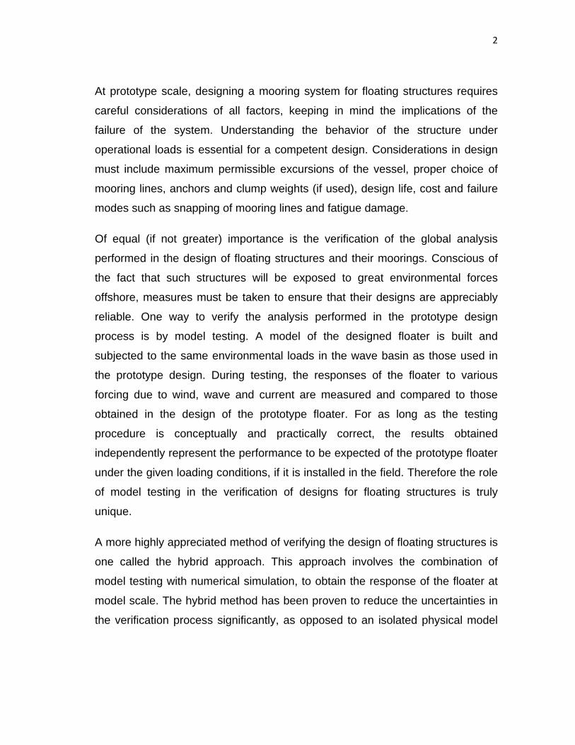
At prototype scale, designing a mooring system for floating structures requires
careful considerations of all factors, keeping in mind the implications of the
failure of the system. Understanding the behavior of the structure under
operational loads is essential for a competent design. Considerations in design
must include maximum permissible excursions of the vessel, proper choice of
mooring lines, anchors and clump weights (if used), design life, cost and failure
modes such as snapping of mooring lines and fatigue damage.
Of equal (if not greater) importance is the verification of the global analysis
performed in the design of floating structures and their moorings. Conscious of
the fact that such structures will be exposed to great environmental forces
offshore, measures must be taken to ensure that their designs are appreciably
reliable. One way to verify the analysis performed in the prototype design
process is by model testing. A model of the designed floater is built and
subjected to the same environmental loads in the wave basin as those used in
the prototype design. During testing, the responses of the floater to various
forcing due to wind, wave and current are measured and compared to those
obtained in the design of the prototype floater. For as long as the testing
procedure is conceptually and practically correct, the results obtained
independently represent the performance to be expected of the prototype floater
under the given loading conditions, if it is installed in the field. Therefore the role
of model testing in the verification of designs for floating structures is truly
unique.
A more highly appreciated method of verifying the design of floating structures is
one called the hybrid approach. This approach involves the combination of
model testing with numerical simulation, to obtain the response of the floater at
model scale. The hybrid method has been proven to reduce the uncertainties in
the verification process significantly, as opposed to an isolated physical model

3
testing approach. Details of the hybrid approach are given in section 1.3.1 of this
document.
Conducting model tests requires wave basins, which are typically limited in
depth and spatial dimensions. Although the model floater is typically much
smaller than the prototype system, depending on the model scale chosen, basin
dimensions may not be sufficiently large to accommodate the directly scaled
mooring system. Consequently, the size of the floater and the accompanying
mooring system are reduced such that they adequately fit into the test facility.
The test engineer has a primary task to replicate the static behavior of the
prototype system on the model to be tested in the wave basin. Essentially, the
effects of the mooring system in the wave basin on the model floater must be
equal to those which the prototype mooring system has on the full-depth floater.
This introduces the need for equivalent mooring systems to represent the
moorings of the full depth system. In many publications, the terms “equivalent
mooring systems” and “truncated mooring systems” are interchangeably used,
but doing so defiles their individual definitions. In a later section of this report, a
proper distinction between the two is drawn for clarity.
1.2 OBJECTIVE OF RESEARCH
The challenge of understanding the behavior of a floating structure under
environmental loads is quite a hand full, and producing designs of mooring
systems with high integrity requires the ability to isolate the various behaviors of
the system as induced by different loads acting. The dynamic response of a
vessel would most often over-shadow its static response. For this reason, it is
considered good practice to study the static and dynamic responses of floating
vessels independently in design, to allow a clear attribution of observed results
to the correct vessel responses.

4
It is therefore pertinent to resort to physical model tests as an important aspect
of the design of offshore structures. Model tests provide a competent approach
to validate computer-aided designs of mooring systems. However, a major
challenge to model testing is the limited depth and dimension of available model
basins. This limitation poses the challenge of developing truncated mooring
systems of static equivalence to that which the considered full depth floaters will
be connected. The designer thus ensures through this process that the static
global behavior of the prototype floater mooring system is most appropriately
represented. Without this representation, the basis for comparing the two
systems (prototype and model) is compromised, and so static equivalence
provides an agreement in static global responses between model and prototype
prior to measurement of dynamic responses.
This research provides a designer-friendly software / program for the design of
statically equivalent mooring systems for model testing purposes. The reader will
find in this text discussions portraying the relevance of suitable software in the
design of such mooring systems. Although many softwares exist that perform
static analysis of mooring systems, most are by far more cumbersome to use for
the mentioned objective. While the designer seeks an optimum statically
equivalent mooring system that reflects a replication of the prototype floating
vessel, flexibility is required in computer-aided design for easy alteration of
design parameters for sensitivity analysis.
General discussions on mooring of offshore structures can be found later in this
chapter, including mooring lines, mooring components and various offshore
mooring systems in contemporary use. The second chapter of this text
discusses previous works related to model testing using equivalent mooring
systems, exposing further the relevance of this research. Within the third
chapter, discussions on the formulation of the software produced in this research
can be found. The application of the formulated tool in the design of statically

5
equivalent mooring systems using possible test cases is reported in the fourth
chapter. Comparisons are also made with existing programs widely used in
mooring analysis. A summary and conclusions follow in the last chapter of this
text, highlighting the economic significance of this project and probable future
modifications to the software.
1.3 TRUNCATED VERSUS EQUIVALENT MOORING SYSTEMS
Throughout this text a truncated mooring systems refers to a mooring system
which has been reduced in size due to basin depth or spatial limitations as
suggested by fig 1.1. In other words the actual mooring system is shortened to
allow physical model testing, used in the verification of design of any considered
floating structure. It is worthy of emphasis that though the truncation of mooring
systems is inevitable based on spatial limitations, the optimum objective is to
have the model’s mooring system produce an equivalent performance to the
already-designed prototype system. Therefore a mooring system which has
been reduced in size and which matches the static properties of the full depth
system in the same number of rigid body degrees of freedom and over some
specified range of loads or offsets is best described as a “statically equivalent
mooring system”. Such a system is the focus of this research, and beyond this
point, it shall in some contexts within this text be simply referred to as an
“equivalent mooring system”. An equivalent mooring system used in model tests
makes the following tasks achievable:
• A demonstration of the competence of the applied concepts in analysis
and design of the mooring system
• Exposing and isolating the system behaviors (dynamic and static), to
enable accurate attribution of various results to the correct loads inducing
them
• Evaluation of the accuracy of assumptions, factors and allowances
considered in the analysis and design process for floating systems

6
• Identification of possible unexpected behaviors of the system, which may
not be accounted-for in the design.
A truncated mooring system simply implies terminating the mooring at the
available depth without modifying the properties of the retained segments. With
such a system, static equivalence is impossible hence the need to modify the
properties of the retained segments to obtain static behaviors similar to those of
the prototype floater.
Fig. 1.1: Sketch of truncated and full depth mooring systems
It is necessary to mention that the successful verification of designs using model
testing with equivalent mooring systems requires competent tools and
experienced testing engineers. Even with such tools and competent engineers,
there may be design issues that cannot be predicted by model testing with a
high degree of accuracy. This implies that numerical simulation models must be
validated and calibrated using conditions as close as possible to the original (full
depth) system. Once this is guaranteed, extrapolation to the full depth system
using the validated model is justified.
Considering that the use of both model testing and numerical simulation together
will increase the tendency to produce more optimal and reliable designs, the
argument that simulation softwares be as designer-friendly as possible is
Full depth
Truncated depth

7
bolstered. A reduction in the complexity of numerical simulation software
reduces the probability of producing incorrect calibration results. If calibration
results are inaccurate, then the basis for comparison of computer-aided designs
with the results of model testing using equivalent mooring systems is almost
completely flawed and this research is essentially aimed at providing a tool
which focuses only on static design, making it easier to formulate a fit-for-
purpose tool.
Certain criteria must be satisfied for a numerical model to be considered
validated by a calibration process; in comparison with model test results
obtained using equivalent mooring systems.
• If the target of the numerical model is to simulate static response of the
floater / mooring system, then it must be able to reproduce all statically
measured responses (global restoring forces, horizontal offsets, tensions,
etc.) from offset tests performed with the same conditions used in the
numerical model simulation.
• For the simulation of dynamic response, the coupled numerical model
should be able to reproduce measured floater / mooring system
responses of damping tests, wind / current forces, regular waves and
random wave tests.
In validating numerical models with model testing, it is important to identify and
apply a testing procedure that assists the verification process. A widely accepted
procedure is to start off with static offset tests, then damping tests, force
calibration tests, regular wave tests, and so on.
1.3.1 DESIGN CONSIDERATIONS FOR EQUIVALENT MOORING SYSTEMS
Discussions here reflect contributions from a wealth of experienced design and
model testing engineers, some of whose works are discussed in the literature
review (second chapter). Important aspects of the verification of mooring

8
designs for deep water floating structures are described. After the scaled
physical model of the floater / mooring system is built, a numerical model of this
physical model is built with the same numerical modeling procedures as the
prototype system. This process is described as “modeling the model”. The
design of the statically equivalent mooring system is performed in such a
manner as to optimize the “needs” for static equivalence of the model system to
be used in the testing project.
System verification tests then proceed and all observations of system
parameters that deviate from the initial model-of-the-model are incorporated in
the model, thereby updating it to meet the “as-built” conditions. The integrity of
the updating process depends greatly on the ability to identify inconsistencies in
the numerical and physical models. Discrepancies may be found in parameters
such as static offsets (for statics tests) and free vibration behavior of floater,
wave radiation and diffraction effects (for dynamics tests). Feeding a correction
of these discrepancies back into the equivalent design model increases the
accuracy of model testing. After the tests are concluded the measured
responses at model scale are extrapolated to the full depth size of the floater /
mooring system using the model-of-the-model, for comparison with the response
from the design of the prototype floater system. The “modeling-the-model”
process is depicted as part of fig.1.2.
An important parameter to be considered in the development options for
equivalent mooring systems is the ratio between the truncated depth (measured
from the fairlead or top attachment point) and the full (original) water depth of the
designed system. This parameter is defined as the truncation factor, and is
denotedγ .
Truncation factor ( )Truncated
Full
WaterDepthWaterDepth
=γ (1.1)

9
The truncation factor is used in computations that guide the selection of mooring
components for equivalent mooring design. An example is the computation of
the total length of equivalent mooring lines equivalenttotalL _ , as:
fulltotalequivalenttotal LL __ *γ= (1.2)
where fulltotalL _ is the total length of the mooring lines at full depth.
Considering the modeling process described earlier, designing an equivalent
mooring system can be described as an optimization process, the results of
which are known before the analysis. The designer faces the challenge of
selecting a combination of mooring components with specific properties that
produce the same static results (global restoring forces and static stiffness) for
the equivalent mooring system as in the prototype system, at least with
acceptable tolerance errors.
Certain factors not considered in the optimization process, but which are usually
accounted for in the making of engineering judgments while comparing the
measured response from model tests to those of the prototype design of the
floater, include the following:
• Uncertainties regarding the model scale and those introduced by the
truncation of the system.
• Interaction effects between mooring system and floater motions.
• Possibility of unknown effects.
• Checking which loading effects are predominant under applied /
prevailing conditions.
It is important to further explain the hybrid approach of design verification, and in
doing so emphasize how this research affects this approach. The explanations
that follow are intended to offer a more explicit understanding of the processes
in fig.1.2.

10
Fig. 1.2: The hybrid approach to design verification Source: Stansberg and others [1]
• After acquiring the design information on the prototype floater (the design
of which is to be verified) pre-test analyses are performed to obtain the
criteria on static and dynamic parameters which must also apply to the
model to be tested. Such parameters will typically include static global
restoring forces and global stiffness in some specified number of rigid
body degrees of freedom, and over some specified loads or offsets. Other
parameters typically included are natural frequencies of the free vibration
of the floater.
• Designing the statically equivalent mooring system follows. It is possible
to use the same numerical tool to both model the model which is to be
tested, and design the statically equivalent mooring system. However,

11
this research is providing a fit-for-purpose tool to handle the design of the
equivalent system. At this point one may consider this development to be
a division of tasks, which will not only increase the accuracy of the results
from each task, but also increase the efficiency of the design process.
• With the designed statically equivalent mooring system in place with the
model floater in the wave basin, model testing commences. A competent
numerical tool is used to represent the floater model, and this numerical
model is validated and updated to include known observed deviations
from the target conditions to which the model floater must comply.
Updates to the model of the statically equivalent mooring system are
generally required to account for deviations between designed and as-
built mooring components (springs, chains, etc.) and other adjustments to
the mooring system to compensate for imperfections in the model floater
(weight, buoyancy, trim). In addition the updating process relies on a
verification of the agreement between the physical model and numerical
model in dynamic effects such as free vibration behavior, as well as linear
wave radiation and diffraction effects. Response data is also collected
independent of the numerical software used in modeling the model.
• At the end of the testing process, the responses simulated by the
validated numerical model should be essentially the same as those
collected independent of the numerical tool. Using the validated / updated
numerical model, post-test analyses involving the extrapolation of results
to predict responses at the prototype scale are performed. The
extrapolated responses are then compared to the responses obtained for
the designed prototype floater.
So the primary effect of this research on the hybrid modeling process is
providing a numerical tool (the development of which is described herein) to
design the statically equivalent mooring system. This implies that a separate
numerical tool would be needed to model the model.

12
Applying the hybrid method of model testing and numerical modeling to the
design of equivalent mooring systems in such a manner that a reliable
verification is performed involves some simplifying assumptions. These
assumptions include:
• The method of analysis adopted in modeling-the-model accurately
replicates the model test performed. One with appreciable level of
experience in model testing and design of equivalent mooring systems
would agree that this assumption is not farfetched if modeling tools are
competent.
• Primary system responses produced by the equivalent mooring system
are large enough to be measured for the validation and calibration of the
analytical models.
• Extrapolation of model outputs to prototype water depth is performed
using accurate numerical schemes.
• No unknowns occur between the equivalent moorings at model test water
depth and the prototype mooring system at full depth.
Compensating for these assumptions in the design of truncated mooring
systems is almost impossible. This gives a feel for the fact that there are
limitations to the hybrid approach of FPS design verification, and that the
integrity of the verification process depends greatly on how well the risks of
errors and uncertainties are reduced. Most problems encountered in the
modeling process associated with the design of these systems are due to
practical imperfections rather than scale effects. As such there will be a variation
in the integrity of different design projects involving testing engineers with
comparable levels of experience.

13
Fig. 1.3: Discrepancies between full depth floater and model scale floater Source: Experimental methods in marine hydrodynamics (NTNU) [2]
Fig. 1.4: Sketch of discrepancies between full depth and model scale systems
The truncation (not equivalence) of a mooring system at model scale can induce
discrepancies compared to the prototype system. To illustrate some
discrepancies between a full depth floater-mooring system and a truncated
system which are inherently existent in design, the floating structures in figs. 1.3
and 1.4 may be considered. The semi-submersible platform in fig.1.4
Full Depth Truncated

14
experiences a horizontal offset as well as rolling motions in the vertical plane.
Clearly, the vessel roll response is magnified in the truncated system with
respect to the full depth system. Designing statically equivalent deepwater
mooring systems thus requires making sound engineering judgments in an effort
to compensate for such lapses.
In view of the tools and limitations discussed, the requirements and alternatives
in deep water model test projects should be considered simultaneously.
Selecting an acceptable verification method may depend on several factors
including the type of floating structure to be modeled, the type of mooring
system to be used, the primary parameters of interest and the environmental
conditions. Typical alternative testing methods in the design of mooring systems
include:
• Ultra small scale testing of complete system; achievable in wave basins.
• Outdoor testing in fjords or lakes. The major limitation in the use of this
method is that the environmental conditions given by nature are
uncontrollable and can therefore not be used on a routine basis as a
verification tool. However, with outdoor testing the compromise on scale
and system simplifications is greatly reduced.
• Hybrid method, combining model testing with numerical modeling - the
steps of which have been appreciably discussed earlier in this section.
1.3.2 MAJOR PARAMETERS IN DESIGN OF STATICALLY EQUIVALENT DEEPWATER MOORING SYSTEMS
In general, the parameters of great significance in the design of statically
equivalent mooring systems are listed below.
• Vertical calm water equilibrium position of the floater in wave basin
• Horizontal offset of floating structure in response to prevailing static loads
• Design water depth (at wave basin scale)

15
• Mooring line characteristics (axial stiffness, submerged weight, length)
• Total global horizontal and vertical restoring forces exerted by mooring
system
• Hydrostatic and mooring contributions to the stiffness matrix for the
floating structure.
Depending on the designer’s interest, some parameters are of greater
significance than others in specific projects. Considering that this research
addresses static equivalence, dynamic parameters are not at play. Having the
capability to understand the effect that each parameter has on the overall design
is interesting. Sensitivity analyses ensure optimum design, and with such
capability optimal design outputs can be obtained and the most critical aspects
of interest in a given project can be addressed. Using such analysis guides the
compensation of a non-equivalent parameter to achieve a desired response. For
instance, in an effort to obtain the correct natural periods of the statically
equivalent floater-mooring system, if the correct pitch stiffness cannot be
achieved and the designer considers this to be important for the floater
response, then an option may be considered where the pitch stability could be
used to compensate inadequate pitch stiffness. In other words, if the longitudinal
metacentric height ( LGM ) of the structure is great enough such that the pitch
motions do not affect the stability of the floating structure, then this effect could
compensate the inadequate pitch stiffness. Although such improvising strategies
are acceptable to some testing engineers, they may not necessarily qualify as
decent practice to others. Overall, the global behavior of the floater is the
deciding factor – this cannot be compromised, regardless of the strategies used
in attaining equivalence.
The reader may have observed that “clump weights” or “clump masses” is not
included in the list of parameters considered in the design of equivalent mooring
systems. Experienced designers consider modeling with clump weights “not

16
ideal”. An even distribution of mooring lines and properties makes modeling
easy and the validation and calibration processes of numerical models is greatly
simplified if clump weights are not used. Without the use of clump weights, there
is also less complexity in the extrapolation of the modeled system responses to
the full system depth.
1.3.3 SCALE AND TRUNCATION FACTOR IN MODEL TESTING
An important issue in model testing using equivalent mooring systems is “scaling
effects”. Satisfying the non-dimensional numbers (Reynolds’, Froude’s and
Strouhal’s) simultaneously at model and prototype scales is practically
impossible. This implies that dimensional similitude often times cannot be
achieved, and that the ratios between the forces acting on the floater-mooring
system will be different at model and prototype scale. Scaling effects refer to the
differences that arise between forces on or motion of the model system, and the
corresponding forces or motions of the prototype system.
Effects of drag forces on slender cylindrical members are generally considered
the most critical scaling effects in model testing. Mooring lines are important
cylindrical members of floating production systems, along with risers. These
drag forces generally depend on Reynolds’ number and the surface roughness
of the cylinder. On the other hand, Froude’s number is considered the most
important dimensionless number in model testing involving gravity waves and is
used as the basis for scaling such model tests. The application of Froude’s
number introduces scale effects as it has no compliance with Reynolds’ and
Strouhal’s numbers.
To address scaling effects in a way that reduces its complexity, choices must be
made based on the relative importance of the forces applicable to the project
under consideration. The designer has to determine which dimensionless
number will control the scaling of the model tests. Hydrodynamic design will

17
most often require the application of Froude’s number, as wave and current
forces are the most prevalent forces that drive the design. This may not
necessarily be the case for the static design of the floater-mooring system. In
general, with respect to the choice of scale the following apply:
• An increase in the scale allows the designer to model the interactions
between the free (water) surface and the floating structure better.
• As the truncation factor increases, it becomes more difficult to achieve
acceptable equivalence between the full depth system and the truncated
system.
• Additionally, as the scale is increased (i.e. scale factor is reduced) the
truncation factor increases. A schematic illustration of how the
uncertainty of the verification process depends on the model scale as
well as the degree of truncation is shown in fig 1.5.
Fig. 1.5: Dependence of uncertainties on model scale Source: Stansberg [1]
The figure describes qualitatively how a large scale model can lead to large
uncertainties due to truncation, and how a small scale can lead to uncertainties
Truncation andnumerical extrapolation
Physical modellingand testing
Unc
erta
inty
on
resu
lts
Scale factor λ

18
due to small models. It is therefore important to operate within an optimal scale
range where the total uncertainties are minimal. In the verification process
discussed in earlier sections, the numerical tools which are part of the hybrid
approach can curb the risk of these uncertainties on the design results, provided
that such tools are efficient and accurate in designing the statically equivalent
mooring system and modeling the tested floater model. This again emphasizes
the need for the use of competent software for such verification processes.
A number of practical issues arise in model testing involving statically equivalent
mooring systems with very small scales (in the order of 100>λ ). Most of these
effects are related to the dynamics of the system, but in this text emphasis is
made only on the issues related to the system statics. A major effect is that
small offsets in the force transducers can lead to large apparent static loads. If
this occurs, measurements of offsets during testing will hardly be accurate, and
it will become necessary to quantify the magnitude of the resulting response due
to the apparent static loads.
A typical range of model scales for equivalent mooring systems is 1:50 – 1:70. In
most cases, it is preferred that these scales cover the modeling of the complete
floater system with moorings and risers. Within this range of scales, scaling
effects are reduced and hydrodynamic effects are modeled more accurately.
Some hold that studies done on certain types of platforms show that model
testing in ultra small scales down to 1:150 – 1:170 is in fact possible, at least for
motions and mooring line forces on such floaters under severe weather
conditions. Other experienced model testing engineers have strong doubts
about the integrity of tests conducted at such small scales. However, the
maximum or minimum scale used in testing will depend on the available basin
dimensions, wave and current generation system, among other factors.

19
1.3.4 PRACTICAL ISSUES IN EQUIVALENT MOORING DESIGN
Another reason for which concise software is needed in the design of statically
equivalent mooring systems is that practical limitations are difficult to account for
when using complex programs in analysis. The practical limitations of small
scale testing must be recognized whenever model testing is done. Even though
most tests are directed toward wave-induced effects such as platform motions
and sea-keeping characteristics, knowing the static mooring response is also
important in design.
One practical problem frequently encountered when modeling the static
response of a vessel is the mismatch in model and prototype static responses,
generated by the rapid change in model mooring line departure angle, compared
to the prototype, for a comparable scaled displacement. For an equivalent
mooring system similar to that shown in fig. 1.6, one cause of this mismatch
could be the closeness of the line-turning pulley to the platform, compared to the
bottom connection point of the prototype system. This problem could very well
occur even if the scaled spring rates were matched for the equilibrium position
(the position of the vessel with no environmental forces present). A schematic
depicting the practical arrangement of this problem is shown in fig 1.6. The
mismatch is illustrated in fig. 1.7 where the total mooring reaction has been
resolved into horizontal surge and sway reactions and a vertical reaction.

20
Fig. 1.6: Model tank station-keeping equipment Source: Mcnatt [3]

21
Fig. 1.7: Static mooring line responses - prototype versus model Source: Mcnatt [3]

22
Another issue is the use of point masses to obtain sufficiently large vertical top
forces, especially with large truncation factors. If point masses are used, the
possible additional dynamic effects need to be checked. Figure 1.8 shows an
example of the use of point masses for a CALM buoy.
Fig. 1.8: A sketch showing the use of point masses in truncated systems
In the system shown in fig. 1.8 the mooring lines and risers are truncated just
above the basin floor such that the characteristics of the truncated system are as
close as possible to those of the full-depth system. However, only a short stretch
of the lines can be modeled with this arrangement. This results in a pretension
that is too low because not all of the weight is accounted for. To correct this
problem the location of the point masses could be adjusted to obtain the correct
pretensions, but this is not applicable to systems with large truncation factors.
For large truncation factors, the geometrical stiffness will be too high if the top
tension is maintained. One option which could be used to obviate this problem
for systems with large truncation factors is to insert a coil spring between the
masses (M1 and M2) to obtain a sufficiently low horizontal stiffness.
Basin wall Water
Steel wire
M1 M2
Buoy
Riser
Steel wire
Basin floor

23
In the design of equivalent mooring systems it is necessary to ensure that
physical characteristics of the prototype mooring system are reproduced in that
of the model, such that the effects of the components in both systems are
similar. Physical properties such as submerged unit weight ( w ), buoyancy and
stiffness ( 0EA ) of chain, wire rope etc. are important in the validation of the
numerical simulation, and so must be chosen such that extrapolation to the full
depth system is easier and more accurate. In many robust / sophisticated
numerical simulation codes the major focus is dynamic analyses and so the
programs are generally geared for such. As a result, model assembly and
interpretation of results for simple static analyses is often unnecessarily
cumbersome when using such programs. Therefore more concise programs with
which these variables can be flexibly altered in design and verification
processes, are worth developing.
1.4 SCOPE OF RESEARCH PROJECT
This research project involves the formulation of a simple, efficient, fit-for-
purpose designer-friendly program for the determination of static responses of
moored floating structures, moored with spread mooring systems. The software
produced is aimed at affording design engineers some flexibility in investigating
the static response of equivalent mooring systems under different design
conditions. Programs are compiled for the analysis of single-segment, two-
segment, and three-segment mooring systems to verify the approach to be used
in formulating the software. It is important to consider up to three-segments of
mooring lines when working with equivalent systems, because this ensures the
flexibility of using different line types in an effort to obtain the desired overall
behavior or property of the lines. Considering spatial constraints in wave basins,
it would be impossible to use just one line type that would satisfy the
requirements of all testing projects.

24
To ensure that the user has the opportunity to view static responses during
design on the same interface, the software is formulated using Microsoft Excel
Visual Basic. The package provides the capability to work with spreadsheets
and user-friendly controls used in the execution of the program. Test cases are
considered for single line mooring analysis and global analysis of spread
mooring systems. The results from the program produced through this research
are compared to those from existing programs (LINANL [4], MOORANL [5] and
Orcaflex [6]) with similar capabilities. An equivalent mooring design for a
representative structure that could be tested in the Offshore Technology
Research Center (OTRC) at Texas A&M University is then performed using the
software. The design outputs are compared to those of the prototype system.
Future modifications to the program produced through this research are
discussed as its current limitations are also highlighted.
1.5 MOORING LINES AND COMPONENTS OF MOORING SYSTEMS
Discussions on mooring lines and mooring components are introduced here to
offer the reader some understanding of their specific applications and
engineering behaviors under various operating conditions. It is important to
relate strongly the engineering properties of various mooring lines and
components to the performance of the mooring systems which they constitute.
Some components of mooring systems find better use under certain conditions
than others.
The factors which determine the types of mooring lines and components to use
in a prototype system include durability, compatibility with the global system,
cost, and functionality under the environmental conditions which they will be
operating. However, these factors are not essentially applicable in the selection
of mooring components for equivalent mooring design. Rather, the selection of
the components which constitute the statically equivalent mooring system will

25
depend on the engineering properties required of the mooring lines to attain the
global match in static properties of the model system when compared to that of
the prototype. Design engineers require a broad knowledge of the properties of
these mooring components, to aid the explanation of design results and decision
making.
Fig. 1.9: Stainless steel cable Source: WebRiggingSupply.com
The mooring lines considered for discussion include steel cable (or wire rope),
chain, synthetic fiber (nylon and polyester) rope and springs. Typically, these are
the mooring line types deployed in model testing of deepwater floating
structures. Other mooring components include different types of anchors and
connectors. At model test scales, it may be difficult to appreciate the features of
these mooring components, and so most of the figures presented in this section
are those of prototype systems, but their engineering properties as associated
with both systems are discussed.

26
Fig. 1.10a: Very flexible steel cable Fig. 1.10b: Flexible steel cable Source: WebRiggingSupply.com
Steel cables or wire ropes could be made out of carbon steel or stainless steel.
They find extensive application in deepwater operations due to their high
strength-to-size ratios. Examples of steel cables with different internal structures
are shown in figs. 1.9, 1.10a and 1.10b. Their flexibility is proportional to the
cross-sectional matrix of the internal strands. This type of material can resist
attacks from aquatic inhabitants, thereby reducing risks of physically-induced
failure. Also, steel is a known material with simple properties, making its effect
easy to account for when interpreting results. However, corrosion becomes an
issue in the use of wire ropes after some time, and this reduces the life span of
the mooring line. If large vessel excursions are envisaged for a given project,
then wire ropes may not be the best choice for such cases, as they only
elongate under very high tensions. In the use of wire ropes for equivalent
mooring, corrosion is not an issue, since the testing projects do not last long
enough for such effects to be at play.
Chains are also used in statically equivalent mooring systems, and their unique
characteristic is providing catenary effects in the mooring lines. Chains find
extensive use in shallow and sometimes intermediate-water depth applications.
In deepwater, the weight of chain required for vessel mooring is enormous and

27
expensive constituting the primary reasons for which its application in deepwater
is highly limited. However, wave tanks are typically not that deep; and in general
material costs for model mooring systems are very modest.
Fig. 1.11: Studless mooring chain Source: TEKNA conference on DP and Mooring of Floating Offshore
Units, 2008 [7]
Fig. 1.12: Stud-linked mooring chain Source: www.cmic.cc
The use of chain however ensures a greater life span for prototype mooring
systems and increases strength and abrasion resistance. In addition, due to their
weight, chains increase the resistance to anchor pull, giving the floating unit
28
more stability over the station under extreme weather conditions. Chains could
either be studless or stud-linked (figs. 1.11 and 1.12 respectively) chains. The
former is usually deployed in permanent moorings, while the stud-linked chains
are used in mooring lines which have to be replaced at intervals during the life
span of the facility. For floating structures at full depth, applications of chains as
part of the mooring lines will mostly favor the use of studless chains because of
the uncertainties associated with the performance of stud-linked chains when
they are twisted while carrying axial loads – especially when the stud links are
welded. A discontinuity at the welded joint could cause failure, and many
consider the use of studless chains to be of lower risk. However, the physical
and mechanical properties of such studless chains must satisfy strength
requirements and further requirements against corrosion. Stud-linked chains on
the other hand may be used in model testing without threat.
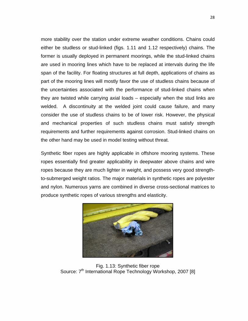
Synthetic fiber ropes are highly applicable in offshore mooring systems. These
ropes essentially find greater applicability in deepwater above chains and wire
ropes because they are much lighter in weight, and possess very good strength-
to-submerged weight ratios. The major materials in synthetic ropes are polyester
and nylon. Numerous yarns are combined in diverse cross-sectional matrices to
produce synthetic ropes of various strengths and elasticity.
Fig. 1.13: Synthetic fiber rope Source: 7th International Rope Technology Workshop, 2007 [8]
29
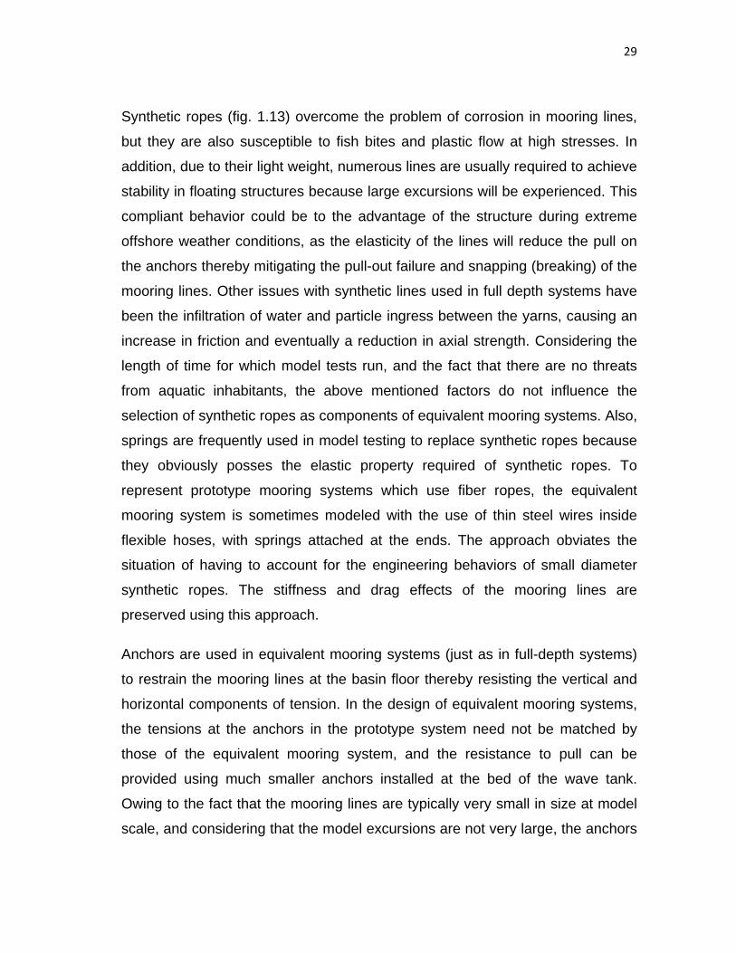
Synthetic ropes (fig. 1.13) overcome the problem of corrosion in mooring lines,
but they are also susceptible to fish bites and plastic flow at high stresses. In
addition, due to their light weight, numerous lines are usually required to achieve
stability in floating structures because large excursions will be experienced. This
compliant behavior could be to the advantage of the structure during extreme
offshore weather conditions, as the elasticity of the lines will reduce the pull on
the anchors thereby mitigating the pull-out failure and snapping (breaking) of the
mooring lines. Other issues with synthetic lines used in full depth systems have
been the infiltration of water and particle ingress between the yarns, causing an
increase in friction and eventually a reduction in axial strength. Considering the
length of time for which model tests run, and the fact that there are no threats
from aquatic inhabitants, the above mentioned factors do not influence the
selection of synthetic ropes as components of equivalent mooring systems. Also,
springs are frequently used in model testing to replace synthetic ropes because
they obviously posses the elastic property required of synthetic ropes. To
represent prototype mooring systems which use fiber ropes, the equivalent
mooring system is sometimes modeled with the use of thin steel wires inside
flexible hoses, with springs attached at the ends. The approach obviates the
situation of having to account for the engineering behaviors of small diameter
synthetic ropes. The stiffness and drag effects of the mooring lines are
preserved using this approach.
Anchors are used in equivalent mooring systems (just as in full-depth systems)
to restrain the mooring lines at the basin floor thereby resisting the vertical and
horizontal components of tension. In the design of equivalent mooring systems,
the tensions at the anchors in the prototype system need not be matched by
those of the equivalent mooring system, and the resistance to pull can be
provided using much smaller anchors installed at the bed of the wave tank.
Owing to the fact that the mooring lines are typically very small in size at model
scale, and considering that the model excursions are not very large, the anchors

30
do not necessarily require embedment at the bottom of the wave tank. Anchors
of adequate weight with the provisions to fasten the mooring lines, such as
shown in figs. 1.14 and 1.15 are appropriate for model testing purposes. Figure
1.14 shows a lead brick of sufficient weight sitting on a metal plate which holds
the line-clamping device. Additional weights may be used but typically the pull
on the anchor is relatively low enough for one or two lead bricks to support.
Fig. 1.14: Anchor set-up for basin scale mooring
Fig. 1.15: Clamping device for basin scale mooring line

31
A side view of the clamping device is shown on fig. 1.15. The bolt on the device
is screwed to hold the wire rope tight in place. If any adjustments to the line
length are required, the bolt is loosened and the rope is pulled in the desired
direction.
Connectors or links such as shown in fig 1.16 could be components of an
equivalent mooring system. Links enable the combination of different mooring
line components having varying properties. The links are tension members,
which in some cases have provision for the installation of floatation to increase
buoyancy effects in the mooring line. Connectors provide an efficient way to
manage the properties of different mooring components such as springs, chain,
cable, etc. while not compromising the integrity of the mooring system. Figure
1.16 shows a connecting link (left) which can be used to connect two line
components of different types (say chain and polyester). The coupled set-up
(right) shows the connection of a wire rope to a screw which may be used at the
terminal point of the line.
Fig. 1.16: Connectors for model scale mooring
Fairleads are important components of mooring systems, provided to guide
mooring lines around the floating structure. In some cases, the floater’s hull
could be built in such a way that the fairleads are holes within the hull, while in
other cases they could be separate pieces of hardware attached to the vessel’s
hull. The bending shoe fairleads (fig 1.17) are simple and less expensive

32
compared to the rotary sheave type, but they also have adverse effects on the
chains when the chains are tensioned. Under this condition, the lying links of the
bending shoe fairlead will be subjected to bending moments; this effect is not
imminent with the rotary type (fig 1.17). At model scale, small sizes of fairlead
types similar to those discussed here may or may not be used. Similar devices
such as pad-eyes and turning rings could also be fabricated during model
building to perform similar tasks as the fairleads, and this is more likely than the
installation of well finished fairleads. The pad-eye screw shown in figure 1.18 is
driven into the hull of the model to serve as the fairlead and the mooring line is
attached to it as in fig 1.16.
Fig. 1.17: Bending shoe and Rotary sheave fairleads Source: Texas A&M Ocean Engineering Seminar [9]

33
Fig. 1.18: Pad-eye screw
It is worthy of mention that the mooring components discussed in this text are
only a few of the existing types used in the model testing processes. Specialized
projects or tasks may warrant the use of unique mooring components which are
peculiar to such projects. Various industries also have patents in manufacturing
specialized equipment for offshore mooring projects, so readers interested in
more elaborate information on a wide range of equivalent deepwater mooring
components should search beyond this text.
1.6 OFFSHORE MOORING SYSTEMS
A coupling of the required mooring components (lines, connectors and anchors)
to the floating structure can be considered a mooring system. This research
focuses on spread mooring systems only, and they can be classified as shown
in fig. 1.19.

34
Spread Mooring System
Conventional Semi-Taut Leg Taut Leg Catenary Catenary
Fig. 1.19: Classification of spread mooring systems
One common capability of systems in fig. 1.19 is that they are all applicable to
deepwater projects. The choice of one over the other in any application depends
on the factors discussed in the introductory section of this chapter. Figure 1.20
illustrates the different types of mooring systems.
Fig. 1.20: Spread mooring systems Source: Texas A&M Ocean Engineering Seminar [9]
Although tendon systems are of great application to some floating structures
(such as TLPs), this research focuses on spread mooring systems which are
applicable to other floater types such as semi-submersible platforms, spars and
FPSOs. Spread mooring systems simply have multiple mooring lines and other
A spar with catenary mooring
A semi‐submersible platform with spread catenary mooring
An FPSO with spread catenary mooring

35
corresponding mooring components necessary for vessel stability. Even though
pre-tensioning individual mooring lines of such systems correctly is fairly
challenging, the vessel excursions are significantly reduced. Practical issues
with spread mooring systems have to do with the entanglement of one line
against another in the event of failure under extreme weather, and the alignment
of the floating structure with the weather.
The conventional catenary system is used in analysis to allow for flexibility in
choice of mooring line properties. With the catenary formulations, the designer
could choose to stiffen or increase the stretch in the mooring lines by altering the
line properties towards the static configurations that correspond to those of the
prototype system. Providing an efficient algorithm to obtain the static equilibrium
solutions for single mooring and spread mooring analysis becomes the next
major concern.

36
CHAPTER II
DESIGN-RELATED LIMITATIONS OF EXISTING MOORING METHODOLOGIES
Quite a number of works have been documented on approaches for design of
equivalent mooring systems and static analysis of spread mooring systems,
some tailored to suit specific cases and others more general. Most of the
existing approaches aim for the same outputs but there may be variations in
methodology (computation techniques) due to efforts made to control
computation durations, increase accuracy of results and / or obtain unique
information from the analysis. From a designer’s perspective, these various
interests are important and the preferred methodology would be one which is
robust enough to capture relevant information on the mechanics of the mooring
system in performance, with a high degree of accuracy and optimum
computation duration.
Given that attaining the objective of this research requires adherence to
acceptable approaches used in model testing as well as mooring line analysis,
the reviews presented in this report can be considered under these two
perspectives. Works related to the present challenges in model testing using
equivalent mooring systems are reviewed first, after which some methodologies
used in mooring analysis are considered. The essence of these reviews is to
justify the need for this research project, and to establish the suitability of the
method used over some of the existing methodologies.
2.1 CHALLENGES IN DEEPWATER MODEL TESTING USING EQUIVALENT
MOORING SYSTEMS
In a study by Kim [10] at the OTRC, FPSO responses in hurricane seas
predicted by a vessel-mooring-riser coupled dynamic analysis program were

37
compared to wave tank measurements. A tanker-based turret-moored FPSO
moored by 12 chain-polyester-chain taut lines in 6,000 ft of water was studied. A
series of model tests (of scale 1:60) were conducted in the OTRC’s wave basin
at Texas A&M University with a statically-equivalent mooring system to assess
its performance in the hurricane condition. In the 1:60-scale OTRC experiment
shown in fig. 2.1, the water depth could not be proportionally scaled as a tank
depth of 100 feet would be required. Therefore, an equivalent mooring system
was developed using steel wires, springs, clump weights, and buoys to
represent the static surge stiffness of the prototype mooring design as closely as
possible. Figure 2.2 (a) shows the mooring system of the prototype system,
while fig. 2.2 (b) shows the equivalent mooring system of the OTRC experiment.
Fig. 2.1: OTRC wave basin and FPSO model Source: Kim [10]
38
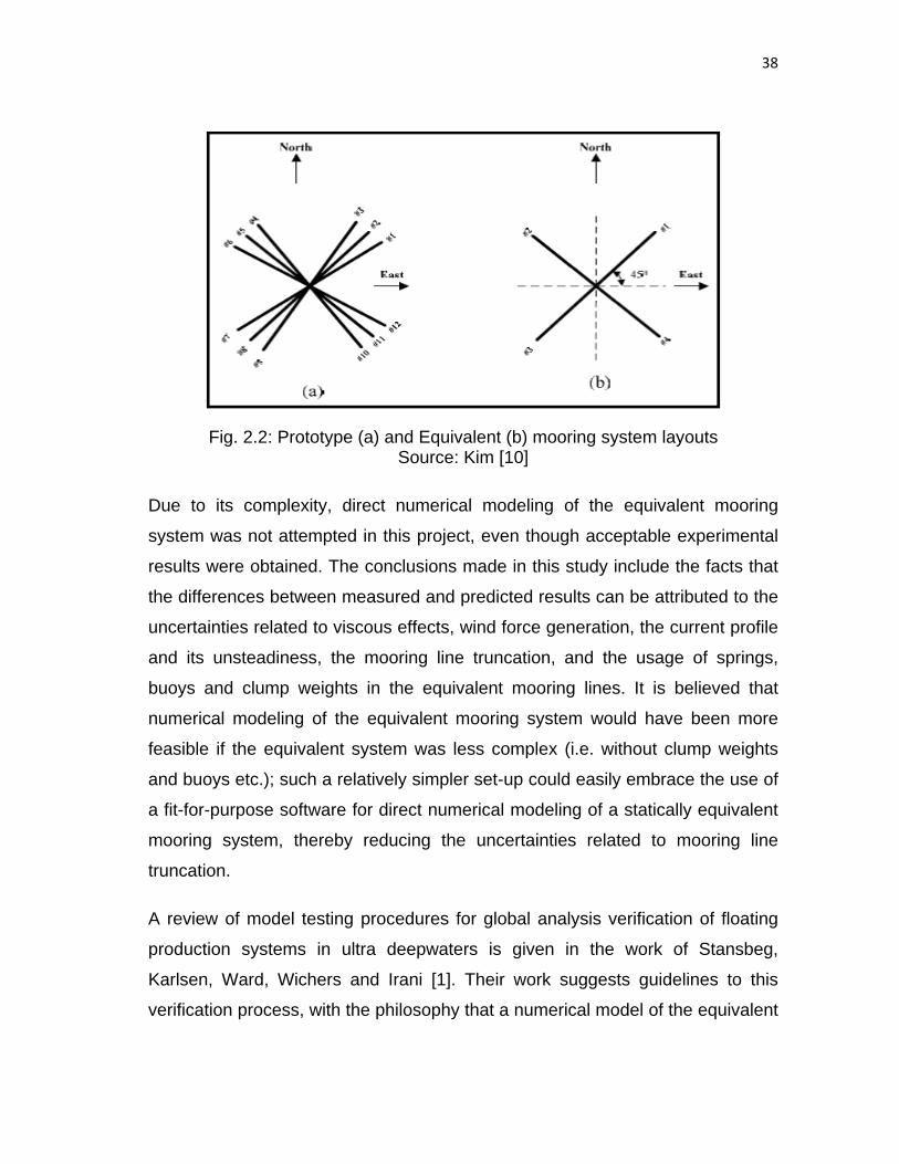
Fig. 2.2: Prototype (a) and Equivalent (b) mooring system layouts Source: Kim [10]
Due to its complexity, direct numerical modeling of the equivalent mooring
system was not attempted in this project, even though acceptable experimental
results were obtained. The conclusions made in this study include the facts that
the differences between measured and predicted results can be attributed to the
uncertainties related to viscous effects, wind force generation, the current profile
and its unsteadiness, the mooring line truncation, and the usage of springs,
buoys and clump weights in the equivalent mooring lines. It is believed that
numerical modeling of the equivalent mooring system would have been more
feasible if the equivalent system was less complex (i.e. without clump weights
and buoys etc.); such a relatively simpler set-up could easily embrace the use of
a fit-for-purpose software for direct numerical modeling of a statically equivalent
mooring system, thereby reducing the uncertainties related to mooring line
truncation.
A review of model testing procedures for global analysis verification of floating
production systems in ultra deepwaters is given in the work of Stansbeg,
Karlsen, Ward, Wichers and Irani [1]. Their work suggests guidelines to this
verification process, with the philosophy that a numerical model of the equivalent

39
set-up is validated against the tests, and the resulting calibration information is
then applied in full-depth verification simulations. Principles for design of
equivalent systems are also discussed. The concerns expressed in their work
include the challenges in model testing, the greatest of all being spatial
limitations in wave tanks. They recommend the hybrid method in which
numerical models are used in the design of statically equivalent mooring
systems and discuss a procedure based on guidelines worked out for DeepStar
as a part of a more general guideline study on global analysis of deepwater
floating production systems [11].
Their recommended guidelines reflect important issues to consider in model
testing using equivalent systems, including the following:
• The most critical response parameters for the floater being tested (e.g.
static or dynamic responses, horizontal or vertical responses etc.)
• When to choose an equivalent system
• Selection of criteria for system truncation
• Degree of system truncation in relation to coupling effects of floater and
underwater systems
• Possibility of equivalent riser modeling
• Response data needed in verifying numerical model, such as slow drift
information (excitation and damping).
Obviously, some considerations in their guidelines pertain to statically
equivalent systems, while others are associated with dynamic equivalence. As
such one may consider their guidelines to be more general. Stansberg and
others [1] also state that the design of an equivalent mooring system should
strive to obtain the same responses of the floater that would result from the full-
depth mooring, in order to reduce the uncertainties related to extrapolation of
test results from equivalent to full-depth systems. Issues further acknowledged

40
include the fact that equivalent mooring systems with more continuously
distributed properties tend to perform better and are easier to analyze.
A truncation case study example is given in their work, where a semi-
submersible platform with 12 catenary mooring lines and 8 risers was tested at
a scale of 1:55 with a full-depth system in 335m depth (fig. 2.3) as well as with
an equivalent system in 167.5m depth (fig. 2.4) of water. It is noted that the
actual water depth in this case is not representative of deepwater, but the idea
was to verify the hybrid approach with equivalent versus full-depth tests, with
both depths included in conventional scale. The statically equivalent mooring
system was selected from static mooring analysis using the computer program
MIMOSA on the basis of comparison of the horizontal restoring force and single
line characteristics versus full-depth. The full-depth lines were of steel wire with
chain segments at the upper and lower parts, while the truncated lines were all
chain. Results presented in fig. 2.5 show a close match in total restoring forces
for the full-depth and equivalent system.
Stansberg and others bolster most of the arguments which form the basis for
this research as discussed in chapter I. However, they offer few leads that
suggest the need for further research on the verification of prototype floater
design using statically equivalent mooring systems. The authors mention the
importance of a good numerical tool for such designs and that such tools must
offer flexible optimization capabilities. Even though the results from MIMOSA
presented can be considered accurate, there is no mention of the efficiency of
the software in the design process. Either way, the authors support the
formulation of flexible design tools that can mimic the full-depth system as
closely as possible, with the argument that such tools would reduce the
uncertainties in the design process.

41
Fig. 2.3: Vertical profile of catenary mooring system – full depth system Source: Stansberg and others [1]
Fig. 2.4: Vertical profile of equivalent system Source: Stansberg and others [1]

42
Fig. 2.5: Total restoring force (in kN) and single line static characteristics of
systems – full depth system versus equivalent Source: Stansberg and others [1]
In an earlier study by Stansberg, Ormberg and Oritsland [12] on the challenges
in deep water experiments, the use of the hybrid method to obviate some of the
uncertainties in the design of statically equivalent mooring systems is explicitly
presented. It is no surprise that the background information in this work is similar
to that of Stansberg and others [1]. They suggest the following rules to be
followed in the design of test set-ups involving statically equivalent mooring
systems:
• Model the correct total, horizontal restoring force characteristic

43
• Model the correct quasi-static coupling between vessel responses (for
example, between surge and pitch for a moored semisubmersible)
• Model a representative level of mooring and riser system current force
• Model the representative single line tension characteristics (at least
quasi-static)
For equivalent mooring systems, modeling the line tension characteristics is not
generally necessary, but it could be useful in confirming that the numerical tool is
producing correct results. The philosophy behind this recommended process is
that the numerical simulations in the modeling process shall take care of the
deviations between the full-depth and equivalent system.
Amongst the enumerated challenges in their work is the need for an efficient
methodology in the design of equivalent mooring systems, such as the
application of an optimization technique to establish the equivalent system with
the required system properties. They also identify that faster and more efficient
algorithms are needed, amongst other numerical challenges.
Fylling and Stansberg [13] used a non – linear optimization code to reduce the
manual iteration work in designing statically equivalent mooring systems. They
explain explicitly that the hydrodynamic loads on a floating structure are not
directly influenced by the mooring systems, and therefore tests on smaller water
depths can be used for obtaining hydrodynamic characteristics of the floating
structure. Their work sought to reproduce the environmental loads and the most
important part of the forces from moorings and risers by reproducing the quasi-
static force vectors from individual lines and risers. They emphasize that
contrary to quasi-static characteristics considered, line dynamics are generally
difficult or even impossible to reproduce by truncated models, and must in all
cases be finally verified by a full-depth numerical model. The hybrid verification
method is used in their work. Design requirements for equivalent mooring

44
systems are also stated, much the same as in the work of Stansberg and others
[1, 12].
Formulating the mooring line equivalence as an optimization problem, Fylling
and Stansberg define the objective function to be a weighted difference of the
restoring forces between the full-depth and the equivalent lines calculated at a
number of offset points. The design requirements that are translated to
constraints are as follows:
• Horizontal stiffness
• Vertical stiffness
• Horizontal pre-tension force
• Vertical pre-tension force
• Horizontal distance from fairlead to anchor
• Length of line on sea-bed
• Capacity of mooring lines
It is important to mention that even though Fylling and Stansberg list the
horizontal distance from fairlead to anchor and the length of line on the sea-bed
as constraints, these parameters are actually alterable in the design of
equivalent mooring systems, though there will be limits to the values that can be
assigned to them. They apply a gradient search method which considers only
continuous variables. Using this approach, three types of optimization variables
may be specified:
• Line variable, pretension or distance to anchor.
• Segment variables comprising segment lengths and one to four cross-
section parameters, depending on segment type.
• In the case of discrete buoyancy or clump weight modules, the net
submerged weight can be specified as a variable.

45
A program called MOOROPT_Trunc was used in solving an example model test
problem at a 1:70 scale. The full-depth semi-submersible is moored in a water
depth of 1500m with polyester lines, while the basin depth is 6.43m with the
model carrying wires, springs, dyneema lines, chains and a buoy. The authors
report a close-to-perfect correspondence of the restoring forces and stiffness
between the full-depth and equivalent test set-ups.
Ormberg, Stansberg and Yttervik [14] worked on integrated vessel motion and
mooring analysis in hybrid model testing. They describe a computer program
(RIFLEX-C) for coupled numerical analysis of moored vessels, where the vessel
is integrated as part of a finite element model of the complete mooring / riser
system. Experimental verification of the program is carried out by detailed
numerical reconstructions of time series from model tests with a semi-
submersible floater. Ultimately the program is used in a model test case study
with equivalent moorings. The authors identify that the essential difference
between running RIFLEX-C and a more conventional stationkeeping program
with a quasi-static mooring line tension model is that dynamic tensions can be
simulated by RIFLEX-C whereas a quasi-static model cannot perform such
analyses. In their application of this program to a model test project, it is noted
amongst other conclusions that the total hybrid testing technique with coupled
analysis is quite complex and time-consuming due to finite element
computations and several steps in the computation procedure. This approach is
however reported to produce simulated line tensions, including low-frequency as
well as nonlinear dynamical components that compare reasonably well with
model test measurements. With the constraints mentioned by the authors, the
use of the coupled numerical analysis tool in the design of statically equivalent
mooring systems would seem to be working-too-hard to get the task done. A
review such as this is included here to support the fact that it is time consuming
and unnecessary to consider dynamic computations when the target in design is
static equivalence.

46
In the final report and recommendations to the 22nd ITTC [15], the specialist
committee on deep water mooring emphasizes the need for the improvement of
numerical modeling techniques for model testing. While the committee
appreciates the notion that model testing of moored floating offshore vessels in
waves can be carried out successfully at a scale ratio of 1:170, it is expected
that at such scales practical problems rather than scaling effects seem to be the
limiting factor in testing. Once again, the hybrid method is believed to offer an
interesting solution to the well known scaling law conflict. The committee
suggests that if parts of the mooring system that are most troubled by the scale
effects are replaced by actuators coupled to on-line computational models with
full scale properties, the complete system can to some extent be free from scale
effects. Recommendations to future work include further pursuance of
verification and validation of physical and numerical models, and enhancement
of the hybrid model testing procedure.
The reviewed literature portrays many common facts, all of which directly imply
the need for more research in the model testing procedures and tools using
equivalent mooring systems. In response to this need, the formulation of tools to
obviate the inherent uncertainties in the verification-of-design process while
ensuring that such tools are designer-friendly is to do the least. A convenient
position would be being able to optimize the requirements of a statically
equivalent mooring system, by doing the least amount of work. Much is involved
in achieving such tools, and it is necessary to approach such a goal from a
realistic point of view. “Realistic” because formulating a tool for the design of
dynamically equivalent systems is extremely challenging and the efforts might
outweigh the benefits. On the other hand, with diligent considerations of
acceptable methods with a view to producing accurate designs through an
efficient algorithm and process, formulating a tool for the design of statically
equivalent mooring systems is doable.

47
2.2 SUITABILITY OF EXISTING APPROACHES FOR MOORING LINE
ANALYSIS
Amongst the many analytical and numerical approaches used in solving mooring
line problems, this research considers just one approach. It certainly is worth
questioning why this particular approach is favored above others. To address
the suitability of existing approaches for mooring line analysis, some works are
reviewed here with the intention of examining how applicable their approaches
might be in the static analysis of spread mooring systems as related to statically
equivalent mooring design.
Smith and MacFarlane [16] present four methods to solve catenary equations for
a three-component mooring system, made up of two line segments connected at
a buoy or sinker. The different methods presented are peculiar to specific
configurations of the system. Their analysis assumes that the water depth and
fairlead tensions are given.
Fig. 2.6: Free body diagram of considered mooring system Source: Smith and MacFarlane [16]

48
For the configuration shown in fig 2.6 the static equilibrium between the
touchdown point at the origin of the axes x and y, and the distance s along the
mooring is given by the summation of forces presented as:
( ) ( ) 0ˆˆ0
00 =++− ∫s
stsTfdtT τ (2.1)
where t̂ is the unit tangent in the direction of increasing s , f is the external load
distribution and T is the tension. The external load is given by:
( ) ( ) ( )112111 ssHwwssWwf −−+−+= δ (2.2)
where 1w and 2w are uniform immersed line weights per unit length, 1W is a
concentrated load at the connection point 1, while δ and H are Dirac impulse
and Heaviside step functions. Equations (2.1) and (2.2) are resolved in the x and
y directions (i.e. in the plane of the mooring line) and the resulting equations are
manipulated to obtain the classical catenary equations:
( )ii Txwdxdy α+= 0/sinh
( ) iiii TxwwTy βα ++= 00 /cosh/ (2.3)
( ) iiii TxwwTs γα ++= 00 /sinh/ (2.4)
( )ii ywT β−= (2.5)
where the subscript “ i ” equals 1, 2 for the mooring lines on the intervals
100 sss <≤= , 21 sss ≤≤ and iα , iβ and iγ are integration constants to be
determined from boundary conditions. In their work, the elongation of the line
was included by way of uncertainty in the weight per unit length.
The first method reduces boundary conditions to a system of five equations
which depend on the line properties (length and weights per unit length), the
load at the connection point, as well as H andT . On prescribing these
properties, t is found by iterating through the reduced boundary conditions.

49
A second method is presented, with a specified condition 12 ww ≠ . It considers no
buoy between the lines and is only for a mooring configuration which has only
two component lines with different weights per unit length. The derivations under
this assumption yield a quartic equation in t , with roots that have a closed form
solution. It is emphasized that this method offers no practical advantage over
Laguerre’s iteration which is applied in the third method.
This third method is an extension of the preceding one, with the inclusion of a
buoy or sinker between the lines, and yields a polynomial equation in 0/1 T of
degree eight. The roots of the polynomial are obtained by Laguerre’s iteration
which is considered efficient and rapidly convergent in evaluating the roots of a
polynomial. The fourth method is only an alternative solution sequence to the
third method, with the primary aim of verifying the symbolic equivalence between
the polynomial coefficients using numerical tests.
In the cases examined by Smith and MacFarlane the numerical equations are
derived based on the given configurations. Even though the numerical schemes
used guarantee accurate results, the iteration yields the solution for the derived
equations only. Analyzing say, a two segment line with equal weights per unit
length would require the mathematical derivations of the boundary conditions,
and then the application of the numerical scheme to obtain the solutions. In
addition, the effect of line elongation is an external computation, rather than an
in-built property of the mooring lines. Considering the stiffness of the mooring
lines while developing the equations for analysis would be a more efficient
approach to reduce computation times and errors. Line stiffness is one of the
important parameters which should be available for adjustments to the designer
of an equivalent mooring system. Therefore from a design standpoint, these
methodologies neglect a key instrument that enhances the process of seeking a
match between static design specifications of the prototype and that of the
equivalent mooring system.

50
Carbono, Menezes and Martha [17] present a steady-state genetic algorithm to
solve mooring pattern optimization problems, owing to the fact that traditional
optimization methods fail to efficiently provide reliable results. They describe the
term “genetic algorithm” to refer to any population-based model that uses
several operators (e.g. selection, crossover and mutation) to evolve. Their work
holds that because the distribution of mooring lines is one of the factors directly
affecting the excursions experienced by floating units, the determination of an
optimum mooring pattern results in an optimization problem, whose ultimate goal
is to minimize the displacements of the floating units.
The specific aspects in which genetic algorithms differ from the most common
mathematical programming techniques, they explain, are:
• Genetic algorithms use a population of individuals or solutions instead of
a single design point.
• They work on a codification of the possible solutions instead of the
solutions themselves.
• These algorithms use probabilistic transition rules instead of deterministic
operators.
• Genetic algorithms handle continuous, discrete or mixed optimization
problems, with minor modifications without requiring further information
such as the gradient of the objective function.
Their formulation of the optimization problem expresses the optimum mooring
pattern as an unconstrained continuous optimization problem, shown as:
( ) ( ) ( )[ ]∑ ∑= =
Δ+Δ=Δm
i
m
iiii yxMinimize
1 1
222: ααα (2.6)
Subject :to niii .....1,min1min =≤≤ ααα (2.7)
where ( )nαααα .....,........., 21= is a vector holding the design variables (e.g. the
azimuth of each mooring line); ( )αiΔ is the resulting floating-unit displacement
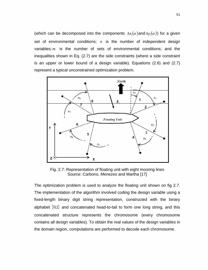
51
(which can be decomposed into the components ( )αixΔ and ( )αiyΔ ) for a given
set of environmental conditions; n is the number of independent design
variables; m is the number of sets of environmental conditions; and the
inequalities shown in Eq. (2.7) are the side constraints (where a side constraint
is an upper or lower bound of a design variable). Equations (2.6) and (2.7)
represent a typical unconstrained optimization problem.
Fig. 2.7: Representation of floating unit with eight mooring lines Source: Carbono, Menezes and Martha [17]
The optimization problem is used to analyze the floating unit shown on fig 2.7.
The implementation of the algorithm involved coding the design variable using a
fixed-length binary digit string representation, constructed with the binary
alphabet { }1,0 and concatenated head-to-tail to form one long string, and this
concatenated structure represents the chromosome (every chromosome
contains all design variables). To obtain the real values of the design variables in
the domain region, computations are performed to decode each chromosome.

52
In computing the static offsets, the environmental loads are transformed into an
equivalent external static force ( )iF acting on the floating structure. The mooring
lines are modeled as non-linear springs that impose restoring forces on the
structure. The restoring forces are obtained through the restoring curves (fig.
2.8) for each mooring line, which are generated using the catenary equation. A
new static equilibrium position is computed (after the out-of-balance forces are
obtained) by solving the following system of non-linear equations:
intRFKd i −= (2.8)
where K is the global stiffness matrix; d is the unknown displacement vector; iF
corresponds to the external forces due to each set of environmental conditions;
and intR is the resultant of the internal (restoring) forces, taking all the mooring
lines into consideration.
Fig. 2.8: Representation of mooring lines by means of non-linear springs Source: Carbono, Menezes and Martha [17]
Evaluating Eq. (2.8) yields a new offset for the floating structure. At this point in
the algorithm the computation is repeated until the resultant of the computed

53
displacements is lower than a specified tolerance – signifying the final static
equilibrium position of the structure. The entire algorithm proposed in their work
is summarized in the following outline.
1. Start
• Initialize parameters
2. Seeding
• Initial population is generated randomly
• Initial population is decoded
• Fitness values of each individual are computed by applying fitness
function
3. Reproduction
• Two chromosomes are selected as parents
• Application of the crossover operator
• Application of the mutation operator
4. Updating
• The two new offspring chromosomes substitute the two worst
chromosomes of the current population
5. Evaluation
• The two chromosomes are decoded
• Fitness of the two new chromosomes is computed
6. Stopping criterion satisfied
• If so, then go to step 7; else go back to step 3
7. Report
8. End
This algorithm has been applied to optimize the mooring pattern of a floating
unit, anchored at eighteen (18) different points. Each mooring line is said to be
composed of three different materials, and the authors report that the algorithm
proved to be robust and effective in analyzing this system. Figures (2.9a) and
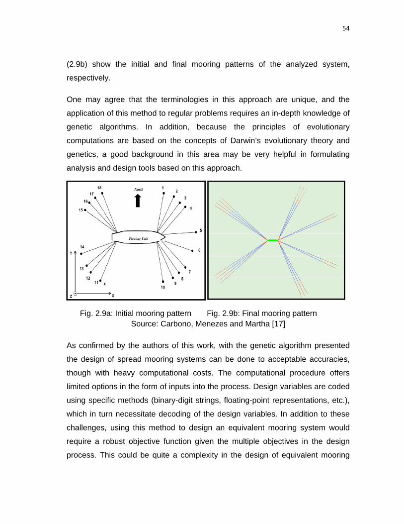
54
(2.9b) show the initial and final mooring patterns of the analyzed system,
respectively.
One may agree that the terminologies in this approach are unique, and the
application of this method to regular problems requires an in-depth knowledge of
genetic algorithms. In addition, because the principles of evolutionary
computations are based on the concepts of Darwin’s evolutionary theory and
genetics, a good background in this area may be very helpful in formulating
analysis and design tools based on this approach.
Fig. 2.9a: Initial mooring pattern Fig. 2.9b: Final mooring pattern Source: Carbono, Menezes and Martha [17]
As confirmed by the authors of this work, with the genetic algorithm presented
the design of spread mooring systems can be done to acceptable accuracies,
though with heavy computational costs. The computational procedure offers
limited options in the form of inputs into the process. Design variables are coded
using specific methods (binary-digit strings, floating-point representations, etc.),
which in turn necessitate decoding of the design variables. In addition to these
challenges, using this method to design an equivalent mooring system would
require a robust objective function given the multiple objectives in the design
process. This could be quite a complexity in the design of equivalent mooring

55
systems, where the design variables are altered continuously to replicate the
static results of the prototype system.
It is important to emphasize the difference between optimizing (or altering)
design variables (or mooring system properties), and numerically searching for
equilibrium using derived equilibrium equations. In the design of equivalent
mooring systems, both optimization of the design parameters and numerical
analysis of the system are inevitable. Selection of mooring system properties
precedes the numerical iterations, but the designer of an equivalent mooring
system is most comfortable with an algorithm which allows swift and repetitive
alternation between these two stages in design. Therefore with the unavoidable
computational complexities in genetic algorithms (which even yield accurate
results), the challenge posed to the equivalent mooring designer is not made
any easier.
The analysis methodology for integrated mooring and riser design was explored
by Connaire, Kavanagh, Ahilan and Goodwin [18]. Their work holds that the
justification for integrated design methods lies in the importance of
hydrodynamic loads, stiffness, damping, added mass and potential compliant
effects of risers as part of a moored system, and also in the need to recognize
the precise station keeping requirements. They developed and investigated
alternative riser and mooring analysis methodologies for five selected floating
production systems, and evaluated the design approaches – this is backed by
the consideration that integrated design of deepwater risers and moorings has
the potential to bring substantial benefits in terms of system response, cost and
safety. Design methods considered in their research represent increasing levels
of complexity and integration of mooring and riser design.
A Central North Sea (CNS) FPSO in 150 meters of water depth, a West of
Shetland (WOS) FPSO in 400 meters of water depth, a Northern North Sea
(NNS) semi-submersible located at 350 meters of water depth, a Brazilian FPSO

56
in 1000 meters of water depth and a generic Gulf of Mexico floating production
unit in 1700 meters of water depth constitute the five vessels used in their
investigation. The first method considered (for each vessel) is a simplified
method which assumes that risers and mooring lines may be represented by an
equivalent vertical cylinder of height equal to the clearance under the keel and
drag diameter equal to that of the actual moorings and risers. Their major
remark about this method is that it is considered appropriate for systems having
negligible riser stiffness, added mass and damping contributions. A second
method, one considered to be of intermediate complexity, considers the
integration of riser stiffness contribution to the overall stiffness of the system. It
involves the calculation of loads on the vessel due to current acting on risers and
mooring lines, and finite element modeling of the risers and moorings to obtain
vessel reaction forces, which are then used to represent the mean vessel load
contribution due to current on the risers and moorings. After explicit modeling
(among other calculations performed) of risers and mooring lines, taking into
account their catenary shape and all inherent material and structural non-
linearities, the riser restoring forces as a function of the position of the riser top
are computed. The horizontal reactions at the top connection opposing the
direction of the applied vessel excursion are evaluated against offset, and the
horizontal reaction versus offset relationship for each riser is then incorporated
in the mooring system. Lastly, their work discusses a final methodology involving
the analysis of a fully integrated three-dimensional, finite element time domain
dynamic riser and mooring system. It is reported that this method implicitly
accounts for all contributions from the risers and mooring lines to the behavior
and response of the entire system.
The reader may have observed that the second method in the work of Connaire
and others is elaborated in this text somewhat more than the first and last
methods. Amongst the three methods, the second method is the recommended
algorithm in their work, and thus the extra attention to the details. Issues

57
acknowledged include the contribution to system stiffness, by considering the
contribution to reduction in vessel excursion for a given static load. Reductions
in static offset due to riser stiffness are presented in Table (2.1) while the
mooring stiffness curve for the Brazilian FPSO is shown on fig. 2.10.
Table 2.1: Comparison of effective system stiffness contribution due to presence
of risers
Vessel Percentage Reduction in Static Offset due to Riser Stiffness
CNS FPSO <1%
WOS FPSO <2%
NNS Semi-submersible Up to 18% in a Single Direction
Brazilian FPSO Approximately 10% in all Directions
GOM FPU 35%
Source: Connaire, Kavanagh, Ahilan and Goodwin [18]
These selected results are included in this text to further expose the capability of
their second algorithm in producing accurate results; therefore lack of accuracy
is not the limitation of this algorithm, in view of using it as a tool in the design of
statically equivalent mooring systems. Figure 2.10 depicts the accuracy of the
algorithm as the analytical results for static offsets produced using the
intermediate (recommended) method match those of model tests with and
without risers.

58
Fig. 2.10: Mooring stiffness curves for the Brazilian FPSO Source: Connaire, Kavanagh, Ahilan and Goodwin [18]
A significant observation in the recommended algorithm is that the computation
procedure flows from the calculation of vessel loads due to dynamic effects, to
the calculation of riser stiffness and other relevant parameters, and finally the
static offsets via mooring analysis, with the inclusion of the effects from all risers
in the system. The authors acknowledge that due to the incorporation of the
risers, there is an influence on the equilibrium of the entire system. Adjustments
to the mooring line pretensions are therefore necessary in order to maintain the
static equilibrium of the vessel, and this adjustment could be critical in terms of
overall restoring force and susceptibility to line dynamic tension amplification.
Considering the use of this algorithm for equivalent mooring design implies the
tedious task of adjusting mooring line tensions to restore the system equilibrium,
for every alternative design configuration (or set of system properties) used to
search for an agreement in design outputs between the model to be tested and
the prototype mooring system. With risers incorporated in the system, the overall
static response depends on more design parameters than if the risers were left
Analytical System With Riser Stiffness Incorporated using Intermediate Approach
Analytical Model Without Risers

59
out. Consequently, isolating the static response of the vessel based on the
mooring system only would be a lot more demanding.
Russell and Lardner [19] performed a statics experiment on an elastic catenary.
Their work is expressed as a variation of the experiments discussed in Irvine
[20] where the change in profile of the catenary line is measured for a small
horizontal cable as additional weights are added at the center and in Irvine and
Sinclair [21] where the weights are added at quarter points. It is highlighted that
the effects of elasticity were negligible in the experiments conducted by Irvine,
and this forms the basis for their experiments to verify the accuracy of the
predictions of the equations of an elastic catenary for a guy wire in which
elasticity is important.
With respect to fig. 2.11 the equations of an elastic catenary (which can also be
found in Irvine [20]) as given in Russell and Lardner are eqns. 2.9 to 2.13.
Fig. 2.11: Free body diagram of elastic cable connecting points A and B Source: Russell and Lardner [19]
In this set-up, the vertical and horizontal distances between the end points of the
cable are l and h respectively. The initial unstrained cable length is L , the
Lagrangian coordinate along the unstrained cable measured from the bottom is

60
s , the horizontal component of the tension H is constant throughout, and the
vertical component of tension at Ls = is V . The elastic modulus and unstrained
cross-sectional area are E and A respectively, while ρ is the weight per unit
length. The cable tension at any point s is given by:
22 )]([)( sLVHsT −−+= ρ (2.9)
The horizontal and vertical coordinates as a function of s are:
⎥⎦
⎤⎢⎣
⎡⎟⎠⎞
⎜⎝⎛ −
−⎟⎠⎞
⎜⎝⎛ −−
+= −−
HLV
HsLVH
EAHssX ρρ
ρ11 sinh)(sinh)( (2.10)
and
⎪⎭
⎪⎬⎫
⎪⎩
⎪⎨⎧
+⎟⎠⎞
⎜⎝⎛ −
−+⎥⎦⎤
⎢⎣⎡ −−
+⎥⎦
⎤⎢⎣
⎡⎟⎠⎞
⎜⎝⎛ −−= 11)(
2)(
22
HLV
HsLVHsLV
EAssZ ρρ
ρρ
(2.11)
respectively.
Applying the boundary conditions lLsX == )( and HLsZ == )( to equations
(2.10 and 2.11) we obtain:
⎥⎦
⎤⎢⎣
⎡⎟⎠⎞
⎜⎝⎛ −
−⎟⎠⎞
⎜⎝⎛+= −−
HLV
HVH
EALHl ρ
ρ11 sinhsinh (2.12)
⎥⎥⎦
⎤
⎢⎢⎣
⎡+⎟
⎠⎞
⎜⎝⎛ −
−+⎟⎠⎞
⎜⎝⎛+⎟
⎠⎞
⎜⎝⎛ −= 11
2
22
HLV
HVHLV
EALh ρ
ρρ (2.13)
Numerical techniques can be used to obtain solutions for equations (2.10) to
(2.13). The authors compare the numerical predictions from the equations of the
elastic catenary with experiments from the guy wire with special interest in the

61
values of tension at the base of the cable for different values of the horizontal
span l . For both horizontal and vertical components, the measured tensions at
the base of the guy wire are reported to be an average of 2.5% lower than the
theoretical values predicted using the elastic catenary equations. It is concluded
that on a scale-model guy wire, the base tensions can be measured to within 5%
accuracy when compared to the predictions from the governing equations.
One interesting characteristic of the elastic catenary equations is the inherent
consideration of line stretch. The effect of EA can easily be controlled as an
input into the equations, rather than an external computation. Additionally, the
simplicity of the equations allows users to control numerical iterations by setting
a known quantity as a boundary condition. These equations deal strictly with the
statics of the system and they offer accurate solutions even at model scale, as in
the case of Russell and Lardner. The parameters do not in any way depend on
the dynamics of the system, and in effect these line properties constitute the
design parameters of interest in statically equivalent mooring systems.
Considering these features of the elastic catenary equations, as long as the
numerical scheme is efficient, it is encouraging to simulate the static
performance of single-segment, two-segment and three-segment mooring
systems with confidence that the results will be accurate as well. It is possible to
code these equations independent of parameters from other submerged
structures connected to the floater (e.g. risers). For these reasons at the least,
the elastic catenary equations are used in the analysis of spread mooring
systems, as applied to this research.
2.3 ENGINEERING BEHAVIOR AND MODES OF FAILURE OF MOORING
LINES
Different mooring lines respond differently to a diverse range of loading
conditions. The properties which they exhibit and the factors surrounding such

62
behavior must be identified and understood by the designer. To satisfy station-
keeping requirements in a full-scale system, the properties that are required for
the design of mooring lines include breaking strength, endurance under cyclic
loading (tension-tension fatigue), durability, dimensions and load-elongation
characteristics. For a clear understanding of the behavior of mooring lines under
varying load conditions, rope testing must be done and the results analyzed.
However, according to Francois [22], whilst some essential tests (such as
breaking strength tests) are usually performed on full size prototypes, other tests
may be omitted when the test results are available from previously qualified
ropes (i.e. ropes which have gone through a full rope qualification process by the
Classification Society).
In model test projects for floating structures, rope testing is not usually an
integral part of the scheme. The selection of mooring lines used in the wave
basin is based on an understanding of the engineering properties of the lines
used in the prototype system, combined with sound engineering judgment.
Components such as springs may be used as equivalent replacement for the
elastic components of the prototype system, while ensuring that the static
outputs of both systems are essentially the same. The performance of mooring
lines at very small scales may vary slightly or significantly from those at large
scales, depending on loading conditions. Such disparities if overlooked may
result in greater challenges during the selection of equivalent mooring
components for design. The notion here is that the more different the
engineering properties of the full scale components are from those of the
equivalent system, the clumsier the optimization process will be in design, or the
more likely that obtaining a good match will be more challenging.

63
2.3.1 ENGINEERING PROPERTIES OF FIBER ROPES
The required minimum breaking strength of a rope is one of the principal
parameters considered in design. Many other parameters used in the design of
station-keeping systems are a function of the breaking strength of the line. For
fiber ropes, at least three samples of rope are tested, and a quantifiable margin
is verified if the breaking strengths of all three samples are above a specified
minimum. A limitation in the 3-tests approach is that the tests will not provide
accurate enough information to adjust the breaking strength from the test results
upward or downward in case of a (marginally) failed test [22]. The breaking
strength should be considered as the basis for a viable check in the performance
of mooring lines even at model scale. Satisfying such conditions will only add to
the integrity of the equivalent mooring design.
Cyclic loading endurance is an important dynamic property of a mooring line,
which offers insight on its response to cyclic tension. Fiber ropes used in deep
water will experience random-amplitude tensions primarily due to wave forces
acting on the floating structure. The endurance of typical polyester ropes has
been quantified for station-keeping, using extensive cyclic loading tests (up to 40
million cycles endurance) performed within the “Rope Durability” project [23],
and found to be far above that of a steel wire rope of the same size. For a
properly designed and manufactured fiber rope, tests indicate that the prevailing
failure mode under such cyclic loading tests is internal abrasion. Other potential
failure mechanisms identified include compression fatigue in synthetic fibers,
slippage in terminations and back-of-the-eye failure. Compression fatigue
however has been found with tests down to 1% minimum loads not to be an
issue [22].
Assessing the durability of any fiber rope involves accounting for all physical
impacts including chaffing, cutting, and internal abrasion by ingress of foreign
materials, which could occur right at the installation phase of the mooring

64
system. The durability of the ropes is directly related to the damages incurred
during the in-service stage. Most cuts (by passing vessels or loose steel wire
ropes) on the fiber ropes are partial; therefore the time to failure is prolonged,
and failure occurs when the load in the line finally exceeds its residual strength.
Assessments made on dropped ropes show that penetration of particles into
fiber ropes is site dependent, and that it is difficult to predict the level of ingress
across the entire length of the rope. The worst case scenario of course, is when
the line is touching the sea floor. Marine growth inside the rope is also strongly
enhanced in such regions while the durability of the rope is reduced.
Francois [22] defines a process called “Bedding-in” as the modification of the
properties of a rope during the first loading(s) and during the early stage of rope
service, pointing out that this behavior is specific to fiber ropes. Bedding-in is
understood to result in the accumulation of permanent elongation and
stabilization of load-elongation properties which are not recoverable unless the
rope is returned to loose (no load) condition for a substantial amount of time.
Francois and Davis [24] proposed a model derived from the results of creep and
recovery tests, to compute the permanent elongation of such ropes as:
PTsuu ppf .+= (2.14)
where PT is the mean (permanent) tension, ps is a flexibility for the long term
elongation ( 10/1=ps is suggested, and PT is in % of the rope MBS), and the
term pu is to be obtained from testing.
The static stiffness of a fiber rope under varying loading conditions depicts the
effect of mean load variations under fluctuating environmental forces. Such
loads may be due to a continuous increase and decrease in a storm or the
existence of loop currents at the station-keeping site. Bureau Veritas [25]
describe a static stiffness test which is depicted in fig 2.12. After a proper

65
bedding-in, the rope is cycled between two tension levels with each half cycle
consisting of a load change (higher or lower) between the two levels. At each
load level there is also a loading plateau during which creep recovery is
measured. The broken red lines in fig 2.12 show the creep deformation stages of
the rope at each loading level. Ultimately, from this test and equations obtained
from the works of Francois and Davies, a prediction can be made of the
elongation over a longer duration of each 2/1 cycle; more representative of
events intended to be modeled.
Fig. 2.12: Static stiffness test Source: Francois [22]
Testing for the dynamic stiffness of fiber ropes involves harmonic loading at
constant amplitude of either load or elongation, about a given mean load.
Francois [22] explains further that testing conditions should include proper
control and measurement of tension using load cells and elongation using gauge
length extensometers. Casey and Banfield [26] have performed long duration
tests and found that the dynamic stiffness in fiber ropes rapidly increases at the
beginning of the run, and then tends to stabilize. They hold however that without
Displacements Measured App
lied loads du
ring
test

66
prior bedding-in, the stiffness continues to increase over durations of hundreds
of thousands of cycles.
Fig. 2.13: Mean load steps and cycling tests Source: Francois [22]
A similar test called the “mean load steps in cycling” test is also discussed in
their work. The loading and unloading sequence for this test is said to be a
single mean-loading cycle consisting of several steps (fig 2.13). The authors
compare the force-strain trend from the “mean load” test to that obtained by
loading the rope at 50% of the minimum breaking strength and to that obtained
from estimates. Details on how the estimated trend is obtained are not provided
in their work and specifics on the loading sequences are also not provided.
However, they observe that there is a relationship between the stiffness increase
and the level of stabilization of the rope, be it creep or recovery, and that in
these tests a complete stabilization is never achieved.

67
2.3.2 PERFORMANCE OF MOORING CHAINS
Mooring systems involving the use of chains show the major loading
mechanisms to be twist (on the vessel attachment), bending (within the fairlead),
highest tensions (just below, or at the fairlead) fatigue (within the arc length of
the line) and wear (towards the end of the line), as illustrated in fig. 2.14.
Fig. 2.14: Loading mechanisms on offshore mooring chains Source: TEKNA Conference on DP and Mooring of Floating Offshore Units [7]
Like any other mooring line type used in offshore operations, chains experience
a range of cyclic tension variations which induce tension fatigue. Figure 2.15
shows examples of chain fatigue. The relationship between the stress range
associated with chains and the number of loading cycles to failure is depicted in
fig 2.16.
Loading mechanisms on offshore mooring chains.

68
Fig. 2.15: Fatigued sections of a mooring chain Source: TEKNA Conference on DP and Mooring of Floating Offshore Units [7]
Fig. 2.16: Stress range - No. of cycles relationship Source: TEKNA Conference on DP and Mooring of Floating Offshore Units [7]
Comparing results from fatigue tests, those obtained from DNV design (OS-
E301) and the DNV-Vicinay approved method for estimating the stress range for
chains as a function of number of cycles, the relationship between the two
parameters follows similar trends. The big picture portrays a reduction in the

69
number of loading cycles until failure as the stress range increases, even though
the DNV-Vicinay method has slightly higher magnitudes for the stress ranges.
2.3.3 BEHAVIOR OF SMALL WIRES
A possible deviation of stretched wires from the simple 2-dimensional catenary
form was investigated by Bowden [27]. His research holds that for real wires,
stretch and bending stiffness modify the catenary form, even for thin wires. The
main effect of stretching, without surprise, is seen to be a reduction in the weight
per unit length. This reduces the wire sag. Bowden gives an expression for the
parabolic approximation for the mid span sag of a stretchable wire as:
( ) 20
11
81
2 lTwly ⎟
⎠⎞
⎜⎝⎛+
−=ε
(2.15)
and the reduced weight per unit length after stretch is given as:
( )ε+= 1/0ww (2.16)
where ( )2ly is the deflection at mid span, w is the initial weight per unit length,
T is the horizontal component of tension in the wire (which is uniform
throughout its length), l is the length of the wire and ε is the strain on the wire.
In an experiment using a 100 meter 0.5 mm diameter wire with Young’s modulus
)207(/10*1.2 23 GPammkgE = , tensioned to kg14 , the wire is found to stretch by
003.0=ε or m3.0 . This strain reduces the deflection by about mm5.0 , an effect
considered to be measurable. At larger scales, similar effects can be expected in
wire ropes used in equivalent moorings for model tests. An understanding of the
behavior of these lines is important in the interpretation of statics results. It
makes it easier to decipher when the outputs are completely different from what
the designer intuitively expects, if such intuition is based on a well informed
perspective regarding the potential behavior of the mooring system components.

70
CHAPTER III
FORMULATION OF STAMOORSYS
With a clear focus on the objectives discussed in earlier chapters,
STAMOORSYS is formulated using governing principles of static analysis of
spread mooring systems. The algorithm applied to obtain the desired results is
concise and easy to comprehend. The software is formulated to allow the
combination of mooring lines of different properties in the mooring system. This
is important in model testing, as the designer may desire to model or represent
the prototype mooring lines with a combination of devices that increase the
tendency of obtaining a match in the static parameters of interest.
STAMOORSYS allows the use of up to 8 mooring lines, all of which can be 3-
segment lines. Modifying the code to accept a different number of lines or a
different number of segments will require a substantial amount of work, as the
user interface will need modification, leading to alterations in almost all cell
references (in Microsoft Excel).
The codes for STAMOORSYS are written using Visual Basic macros in
Microsoft Excel 2007 version. Using this package makes it easy to create an
efficient interface between the codes and the user while retaining the ability to
view results instantly at the end of each analysis. Alternating between different
windows during the design of statically equivalent mooring systems is
completely ruled out, as the design interface is formulated to be self-sufficient
regarding required inputs and desired outputs. By creating the program in
Microsoft Excel, there is the added advantage available to the user to apply the
tools originally embedded in Excel for any desired post-processing analysis
possible with such tools. One of such tools (particularly useful during the design
process) is the ‘scenario manager’ in Excel. The scenario manager is extremely
useful in saving design scenarios for future use. Such tools will also substantially

71
reduce the time required to enter input data for design. It is also possible to save
the spreadsheet and rename it for archival purposes after each design project.
3.1 GENERAL PRINCIPLES IN STATIC ANALYSIS OF SPREAD CATENARY
MOORING SYSTEMS
Given that a spread mooring system comprises several individual catenary
mooring lines, the procedure used in the analysis of a single line forms the basis
for resolving the static parameters of the spread mooring system. The
fundamental principles of system equilibrium apply, and can be expressed in the
following equations:
∑ = 0XF (3.1)
∑ = 0YF (3.2)
∑ = 0ZF (3.3)
Fig. 3.1: Sketch of spread mooring system with 4 mooring lines in elevation

72
Considering fig. 3.1, eqns. (3.1) to (3.3) are the only equilibrium equations of
interest regarding the static equivalence under discussion. Although additional
static equilibrium equations ( 0,0,0 === ∑∑ ∑ ZYX MMM ) could be
considered, the floater is assumed (at the moment) not to rotate, hence moment
equilibrium is not considered. The primary target is to ensure that the static
global horizontal forces and stiffness on the floating vessel in the equivalent
system are close enough to those of the prototype system.
Fig. 3.2: Single-segment mooring
For a single segment mooring under equilibrium conditions such as that shown
in fig. 3.2, the equilibrium equations for static analysis can be derived as shown
in eqns. (3.4) through (3.37). The configuration in fig. 3.2 and the subsequently
derived equations are specifically for the case where the point “ a ” (the left end
of the line) corresponds to the catenary touch-down point or to a point where
there is a vertical uplift component to the tension. It is assumed that the water is
calm, that is, it does not exert a force on the cable (other than buoyancy). The
submerged unit weight of the cable is w (weight per unit length).

73
Considering an isolated elemental length ds of the line in fig. 3.2, the free body
diagram can be drawn as shown in fig 3.3. The tension T at the left end of the
section is replaced by its vertical and horizontal components V and H
respectively, and the submerged weight per unit length is w .
Fig. 3.3: Free body diagram of elemental section
Taking summation of forces in the horizontal axis in fig. 3.3:
∑ = 0XF
0)cos()( =+++− φφ ddTTH (3.4)
Using the identity:
φφφφφφ ddd sinsincoscos)cos( −=+
Equation (3.4) can be written as:
P(x, z; p)
External wall of mooring line

74
[ ] 0sinsincoscos)( =−⋅++− φφφφ dddTTH
0sinsin)(coscos)( =+−++− φφφφ ddTTddTTH
If we assume that φd is small, then 1cos ≈φd and φφ dd ≈sin
0sin)(cos)( =+−++− φφφ ddTTdTTH
0sinsincoscos =−−++− φφφφφφ ddTdTdTTH
Since φcosTH = ,
0sinsincos =−− φφφφφ ddTdTdT
We can consider the third term on the left hand side to be very small relative to
other terms; hence we neglect it to obtain:
0sincos =− φφφ dTdT (3.5)
from which:
φφdTdT tan= (3.6)
Similarly we take the summation of forces in the vertical axis in fig. 3.3:
∑ = 0ZF
0)sin()( =+++−− φφ ddTTwdsV (3.7)
[ ] 0cossincossin)( =+⋅++−− φφφφ dddTTwdsV
Again if we assume that φd is small, then 1cos ≈φd and φφ dd ≈sin

75
wdsdTdT =+ φφφ sincos (3.8)
Substituting eqn. (3.6) into eqn. (3.8)
wdsddT =+ )sintan(cos φφφφφ
If we substitute φcos
HT = and 1sectan 22 −= φφ
we obtain:
wdsdH=φ
φ2cos
Integrating both sides, we have:
∫ ∫= dswdH φφ2cos
1
CsHw
+= φtan (3.9)
At 0=s , aφφ = and therefore aC φtan−=
Therefore eqn. (3.9) can be written as:
aHHws φφ tantan −= (3.10)
which can also be written as:
aHwsV φtan+= (3.11)

76
The magnitude of the tension in the mooring line at point “a” can be expressed
as:
22 VHT +=
Therefore along the mooring line, the tension as a function of arc length can be
expressed in terms of eqn. (3.11) as:
22 )tan()( aHwsHsT φ++= (3.12)
or
2
tan1)( ⎟⎠⎞
⎜⎝⎛ ++= aH
wsHsT φ (3.13)
Equation (3.12) or (3.13) gives the tension distribution along the mooring line.
As in Irvine [28], let s be the Lagrangian coordinate of the un-stretched mooring
line. We can define a point P along this s coordinate. However, under the self
weight of the line (or external loads) the point P moves to occupy a new position
in the stretched configuration of the mooring line described by Cartesian
coordinates zx, and Lagrangian coordinate p . With respect to point P we can
write:
dpdx
=φcos (3.14)
and
dpdz
=φsin (3.15)
So we can write the horizontal component of the tension at point P as:

77
dpdxTH = (3.16)
It is assumed that the elasticity of the mooring line can be modeled by Hooke’s
law as:
00 EAT
LL=
Δ (3.17)
where 0L is the un-stretched length of the line (under no tension), E is the
Young’s modulus of the mooring line and 0A is the effective cross-sectional area
of the mooring line. The ratio of change in length to the original length can also
be expressed as:
10
−=−=Δ
dsdp
dsds
dsdp
LL (3.18)
So from eqns. (3.17) and (3.18)
01 EAdsdpT ⎟
⎠⎞
⎜⎝⎛ −=
10
+=EAT
dsdp (3.19)
The change along the x coordinate with respect to the Lagrangian coordinate s
can be expressed as:
dsdp
dpdx
dsdx
⋅= (3.20)
From eqn. (3.16):

78
TH
dpdx
= (3.21)
Therefore substituting eqns. (3.19) and (3.21) into (3.20), we have:
TH
EAH
EAT
TH
dsdx
+=⎟⎟⎠
⎞⎜⎜⎝
⎛+=
00
1 (3.22)
Substituting eqn. (3.12) in eqn. (3.22), we have:
dswsVH
HdsEAHdx
220 )( ++
+= (3.23)
Recalling that the integral of the form ∫ ⎟⎠⎞
⎜⎝⎛=
+−
axdx
xa1
22sinh1
On integration, eqn. (3.23) becomes:
CH
wsVw
HEAHssx +
⎭⎬⎫
⎩⎨⎧
⎟⎟⎠
⎞⎜⎜⎝
⎛⎟⎠⎞
⎜⎝⎛ +
+= −1
0
sinh1)( (3.24)
At 0)0(,0 == xs , so
⎭⎬⎫
⎩⎨⎧
⎟⎠⎞
⎜⎝⎛−= −
HV
wHC 1sinh
and therefore
⎭⎬⎫
⎩⎨⎧
⎟⎠⎞
⎜⎝⎛−⎟
⎠⎞
⎜⎝⎛ +
+= −−
HV
HwsV
wH
EAHssx 11
0
sinhsinh)( (3.25a)
Equation (3.25a) gives the x coordinate of the mooring line as a function of s .
For an inextensible mooring line ∞→0EA and eqn. (3.25a) reduces to (3.25b):
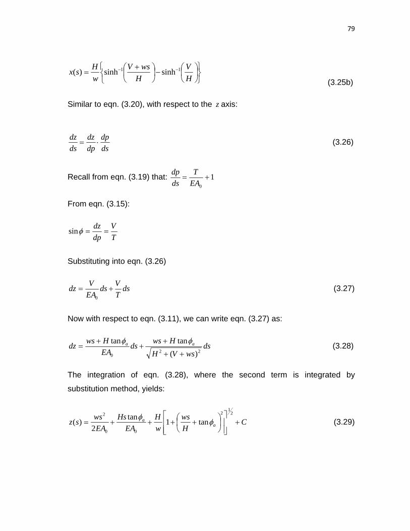
79
⎭⎬⎫
⎩⎨⎧
⎟⎠⎞
⎜⎝⎛−⎟
⎠⎞
⎜⎝⎛ +
= −−
HV
HwsV
wHsx 11 sinhsinh)(
(3.25b)
Similar to eqn. (3.20), with respect to the z axis:
dsdp
dpdz
dsdz
⋅= (3.26)
Recall from eqn. (3.19) that: 10
+=EAT
dsdp
From eqn. (3.15):
TV
dpdz
==φsin
Substituting into eqn. (3.26)
dsTVds
EAVdz +=
0
(3.27)
Now with respect to eqn. (3.11), we can write eqn. (3.27) as:
dswsVH
HwsdsEAHwsdz aa
220 )(
tantan++
++
+=
φφ (3.28)
The integration of eqn. (3.28), where the second term is integrated by
substitution method, yields:
CHws
wH
EAHs
EAwssz a
a +⎥⎥⎦
⎤
⎢⎢⎣
⎡⎟⎠⎞
⎜⎝⎛ ++++=
21
2
00
2
tan1tan2
)( φφ (3.29)

80
At ,0=s 0)0( =z , so
[ ] 0tan1 212 =++ C
wH
aφ
Therefore awHC φsec−=
Equation (3.29) can now be written as:
aaa
wH
Hws
wH
EAHs
EAwssz φφφ sectan1tan
2)(
21
2
00
2
−⎥⎥⎦
⎤
⎢⎢⎣
⎡⎟⎠⎞
⎜⎝⎛ ++++= (3.30)
Therefore the z coordinate of the mooring line as a function of s is given by eqn.
(3.30). For an inextensible mooring line ∞→0EA and eqn. (3.30) reduces to:
⎪⎭
⎪⎬⎫
⎪⎩
⎪⎨⎧
−⎥⎥⎦
⎤
⎢⎢⎣
⎡⎟⎠⎞
⎜⎝⎛ ++= aaH
wswHsz φφ sectan1)(
21
2
(3.31)
We can derive an expression for the arc length s of the mooring line as a
function of the x coordinate, using the governing differential equation of the
catenary. Recalling eqn. (3.10):
aHHws φφ tantan −=
adxdz
Hws φtan−=
(3.32)
Differentiating both sides with respect to x :
2
2
dxzd
Hws
dxd
=⎟⎠⎞
⎜⎝⎛ (3.33)

81
Equation (3.33) is the governing differential equation of the catenary line.
Since 222 )()()( dzdxds += , we can write
[ ] 2121 z
dxds ′+= (3.34)
where dxdzz =′ . (3.35)
Substituting eqn. (3.34) into eqn. (3.33)
[ ] 212
2
2
1 zwdx
zdH ′+=
[ ] 212
2
2
1 zdx
zd
Hw
′+=
[ ]∫∫ ′′+
= zdz
dxHw
2121
1
11sinh Czx
Hw
+′= −
⎟⎠⎞
⎜⎝⎛ −=′ 1sinh Cx
Hwz
211 coshsinh CCxHw
wHCx
Hwz +⎟
⎠⎞
⎜⎝⎛ −=⎟
⎠⎞
⎜⎝⎛ −= ∫
At azx φtan,0 =′= , therefore
)(tansinh 11 aC φ−−=

82
At 0,0 == zx , therefore
))(tancosh(sinh 12 aw
HC φ−−=
Therefore;
( ) ( )( )⎥⎦
⎤⎢⎣
⎡−⎟
⎠⎞
⎜⎝⎛ += −−
aaxHw
wHxz φφ tansinhcoshtansinhcosh)( 11 (3.36)
Equation (3.36) gives the vertical coordinate of a mooring line as a function of x ,
the horizontal coordinate.
From equation (3.32);
( )⎭⎬⎫
⎩⎨⎧
−⎥⎦⎤
⎢⎣⎡ +=⎟
⎠⎞
⎜⎝⎛ −= −
aaa Hwx
wH
dxdz
wHxs φφφ tantansinhsinhtan)( 1 (3.37)
Equation 3.37 gives the arc length of the mooring line as a function of the
horizontal coordinate x . A summary of the major equations used in obtaining
equilibrium solutions for single segment mooring is presented in Table 3.1.
Other equations such as those for )(xs and )(xz may also be used in
determining static equilibrium, but this will depend on the numerical strategy
adopted for the iteration process. To obtain static solutions using the equations
shown in Table 3.1, the following information must be provided:
• The elevation of the top end of the mooring line segment, relative
to the bottom end
• Line weight per unit length w , line length L , axial stiffness 0EA
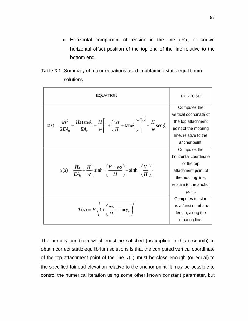
83
• Horizontal component of tension in the line )(H , or known
horizontal offset position of the top end of the line relative to the
bottom end.
Table 3.1: Summary of major equations used in obtaining static equilibrium
solutions
EQUATION
PURPOSE
aaa
wH
Hws
wH
EAHs
EAwssz φφφ sectan1tan
2)(
21
2
00
2
−⎥⎥⎦
⎤
⎢⎢⎣
⎡⎟⎠⎞
⎜⎝⎛ ++++=
Computes the
vertical coordinate of
the top attachment
point of the mooring
line, relative to the
anchor point.
⎭⎬⎫
⎩⎨⎧
⎟⎠⎞
⎜⎝⎛−⎟
⎠⎞
⎜⎝⎛ +
+= −−
HV
HwsV
wH
EAHssx 11
0
sinhsinh)(
Computes the
horizontal coordinate
of the top
attachment point of
the mooring line,
relative to the anchor
point.
2
tan1)( ⎟⎠⎞
⎜⎝⎛ ++= aH
wsHsT φ
Computes tension
as a function of arc
length, along the
mooring line.
The primary condition which must be satisfied (as applied in this research) to
obtain correct static equilibrium solutions is that the computed vertical coordinate
of the top attachment point of the line )(sz must be close enough (or equal) to
the specified fairlead elevation relative to the anchor point. It may be possible to
control the numerical iteration using some other known constant parameter, but

84
the condition stated above is the only one used in this work at this point. Only
after this condition has been satisfied is the horizontal coordinate of the line
computed. In the iteration procedure the angle of the line at the bottom end )( aφ
or the length of the line on seafloor is adjusted until static equilibrium is reached.
For three segment lines, three vertical coordinates are used in the computations.
If the described equilibrium condition is not satisfied after the first vertical
coordinate )( 33 sz (for the third segment) has been computed, then the second
vertical coordinate )( 22 sz is computed and a summation of both first and second
vertical coordinates are compared to the “iteration parameter”, in this case the
fairlead elevation. A summation of all three vertical coordinates is computed and
compared to the iteration parameter, if the condition is not satisfied after the
second comparison. This process is explicitly explained in the following section
and with the aid of a detailed flow chart.
3.2 ALGORITHM USED IN STAMOORSYS FOR THE DESIGN OF
STATICALLY EQUIVALENT SPREAD MOORING SYSTEMS
With the elastic catenary equations and the principles of static equilibrium,
designing the equivalent mooring system requires efficient algorithm that
produces the static solutions efficiently and with high accuracy. Whether the
mooring system is a single component (or single-segment) system or a multi-
segment system, a direct solution cannot be obtained as the problem is highly
nonlinear. The solutions have to be obtained iteratively, using a known quantity
to control the iteration process.
The primary requirement of the design process is to match the global restoring
force versus offset, and the global stiffness versus offset curves for a range of
offsets specified by the user. A combination of line properties selected by the
designer will produce a unique result. If there is no match between the obtained

85
results and the target curves, the designer will have to continue optimizing the
selected components and configurations of the mooring line, in search of a
satisfactory match. It is therefore necessary that the mechanism of computation
be such that results are returned quickly, to allow the efficient management of
the optimization processes by the designer.
Overall, the algorithm used in STAMOORSYS to analyze and design a statically
equivalent spread catenary mooring system is summarized as follows:
• Read input data – anchor and fairlead coordinates, vessel offsets, line
properties, minimum and maximum preliminary restoring forces,
numerical increment value to be used in iteration (i.e. quantity by which
angle at the bottom end of line or length of line on seafloor will be
adjusted numerically) for analysis of all lines (1 to 8).
• For each given offset (as in fig. 3.4) compute the departures (horizontal
distance from anchor to fairlead) in each line, in the plane of the line.
Fig. 3.4: Sketch of single line mooring showing offset and departure
• Given the range of preliminary restoring forces (minimum, maximum and
number of points), compute preliminary departures in the plane of one

86
line using the same line properties to be used in design. The departures
are calculated using an iterative process, which uses the vertical distance
between fairlead and seabed as the conditional parameter.
• Using the known departures in the planes of the respective lines for each
offset, interpolate within the preliminary departures to find the
corresponding restoring forces in the plane of each line.
• Resolve the forces into the Cartesian planes, and apply equilibrium
equations to obtain the static global forces on the vessel.
• Compute the global stiffness in the respective Cartesian planes
Fig. 3.5: A summary of the computation procedure in STAMOORSYS
Read input data (Coordinates, offsets, line properties, etc.)
For each considered offset, compute departures in the plane of the line and new heading of lines after
vessel is given each offset.
Use preliminary restoring forces to compute preliminary departures in the plane of the line. Hold preliminary departures and preliminary restoring forces in archive for interpolation.
Using departures computed for each offset (in step 2 above), interpolate along the preliminary restoring force versus preliminary departures curve, to obtain restoring forces corresponding to these departures, in the plane of the line.
With the local restoring forces obtained through interpolation, perform global analyses to obtain global restoring forces and
global stiffness.

87
The computation procedure just described is depicted in fig. 3.5. It is important
to explore each step in the algorithm in detail, beginning with the reading of input
data. Given that the user interface for STAMOORSYS is hosted in a
spreadsheet, input data is entered into the spreadsheet cells in an orderly array.
On execution of the static analysis using the controls on the user interface, the
Visual Basic macros in Excel call-in the input data from the spreadsheet, and
perform the coded operations.
To calculate the departures in the plane of the lines for each given offset,
several offset cases are considered. STAMOORSYS considers a total of 4
different cases, each of which typically differs in coordinates from the other.
STAMOORSYS regards the center of the platform at the zero-offset position of
the vessel as the origin of the global coordinate system, and all coordinate
inputs are in Cartesian coordinates. A parallel body-fixed coordinate system has
its origin at the center of the platform. In general, the expression for calculating
the departure of the i th mooring line is:
( ) ( )22ii fpoffifpoffii YYYXXXD ±±+±±= (3.38)
In eqn. (3.38) iX is the x-coordinate of the anchor relative to the global
coordinate system, offX is the x-coordinate of the given offset on the vessel
relative to the global coordinate system, and ifpX is the x-coordinate of the
fairlead relative to the body-fixed coordinate system at the center of the platform.
The subscript “ i ” is the line number index. It is clear from eqn. (3.38) that the
magnitude and direction of the given offsets affect the resulting departure. The
different offset cases considered are given in the following bullets, and case 1 is
illustrated in fig. 3.6.
• Case 1: 0,0 == offoff YX

88
• Case 2: 0,0 >= offoff YX
• Case 3: 0,0 => offoff YX
• Case 4: 0,0 >> offoff YX
STAMOORSYS has no restrictions on the locations of lines 1 through 8.
However, the program assumes that all fairleads have the same elevation and
that all anchor points have the same depth. An additional restriction is that for
any line which has one of its anchor coordinates as zero, STAMOORSYS
assumes the corresponding fairlead coordinate in that direction to be zero, for
that line. So for line 2 for instance in the 8-line set-up shown on the right of fig.
3.6, because the x-coordinate of the anchor relative to the center of the platform
is 02 =X , STAMOORSYS will assume that its fairlead attachment point will be
02=fpX .
Fig. 3.6: Sample layout of 4-line and 8-line system for zero offset case

89
As mentioned earlier, computing the preliminary departures to be used in
interpolation for restoring forces is an iterative process. For STAMOORSYS the
numerical iteration process (fig. 3.7) depends on the fairlead elevation as the
specified known quantity. It is important to emphasize the distinction between
adjustable parameters in the numerical analysis and the adjustable design
parameters used to optimize the design. The numerical computation uses the
most sensitive parameters of the quasi-static simulation to adjust the
configuration of the mooring lines, in search for the equilibrium configuration.
These sensitive parameters are the length of line on the seafloor or the angle
which the mooring line makes as it comes in contact with the seafloor. Adjusting
either of these parameters by small amounts until the computed fairlead
elevation is close enough to the given fairlead elevation is the major numerical
strategy.
On the other hand, to optimize the design of the statically equivalent mooring
system, one must consider the physical properties (submerged weight per unit
length, length, and axial stiffness) of the mooring line segments and the
coordinates of the anchor relative to the center of the platform. However,
different combinations of design parameters may increase or reduce
computation times, depending on the probability of attaining static equilibrium
with the selected properties.

90
Assume that all of segment 3 issuspended, and all of segments
1 & 2 are on the seafloor.
Compute angles at intersectionof segments and at fairlead.Compute tensions at anchor,
fairlead, and at intersection ofsegments.
Compute vertical distance fromanchor to fairlead (Z). Comparecomputed value of Z with givenvalue of fairlead elevation (FE).
Z > FE
Adjust length of segment 3 onseafloor, by small increament.
Compute angles at intersections ofsegments and at fairlead. Compute
tensions, suspended length, length onseafloor and vertical distance between
fairlead and anchor.
Compare Z with FE
Z > FE
Z < FE
Compute departure and reportresults.
Z = FE Z < FE
Compute departure and reportresults. Assume that all of segments 2
and 3 are suspended, and all ofsegment 1 is on the seafloor.
Compute angles at intersection ofsegments and at fairlead. Computetensions at anchor, fairlead, and at
intersection of segments.
Compute vertical distance fromanchor to fairlead (Z). Comparecomputed value of Z with givenvalue of fairlead elevation (FE).
Z > FE
Adjust length of segment 2 onseafloor, by small increament.
Compute angles at intersections ofsegments and at fairlead. Compute
tensions, suspended length, length onseafloor and vertical distance between
fairlead and anchor.
Compare Z with FE
Z > FE
Z < FE
Compute departure and reportresults.
Z = FE Z < FE
Compute departure and reportresults.
Assume that all of segments 1,2 and 3 are suspended.
Compute angles at intersection ofsegments and at fairlead. Computetensions at anchor, fairlead, and at
intersection of segments.
Compute vertical distance fromanchor to fairlead (Z). Comparecomputed value of Z with givenvalue of fairlead elevation (FE).
Z > FE
Adjust length of segment 1 onseafloor, by small increament.
Compute angles at intersections of segmentsand at fairlead. Compute tensions, suspendedlength, length on seafloor and vertical distance
between fairlead and anchor.
Compare Z with FE
Z > FE
Z < FE
Compute departure and reportresults.
Z = FE Z < FE
Compute departure and reportresults. Adjust angle which segment 1 makes
with seafloor, by small increament.
Compute angles at intersections ofsegments and at fairlead. Computetensions, suspended length, lengthon seafloor and vertical distance
between fairlead and anchor.
Compare Z with FE
Z > FE
Z < FE
Compute departure and reportresults.
Fig. 3.7: Numerical procedure in STAMOORSYS

91
Fig. 3.8: Simple sketch of 3-segment mooring line
A sketch of a 3-segment mooring line is shown in fig. 3.8. Limiting configurations
of a three-segment single line mooring system are shown on figs. 3.9 through
3.14. The conditional statements depicted in fig. 3.7 are written to search
through the configurations displayed in figs. 3.9 through 3.14 for a coinciding
scenario, within which the sensitive parameters of the quasi-static simulation are
adjusted.
In the STAMOORSYS set-up and design pages, the parameter labeled
‘numerical increment value in iteration’ is the amount by which either the length
of line on the sea floor or the angle which the line makes with the sea floor will
be adjusted in the search for the equilibrium configuration. A value of 0.01 (feet
or meter, or radian) is the recommended default value for analysis in
STAMOORSYS. A value smaller than the recommended value will yield more
accurate results but at the cost of simulation time.
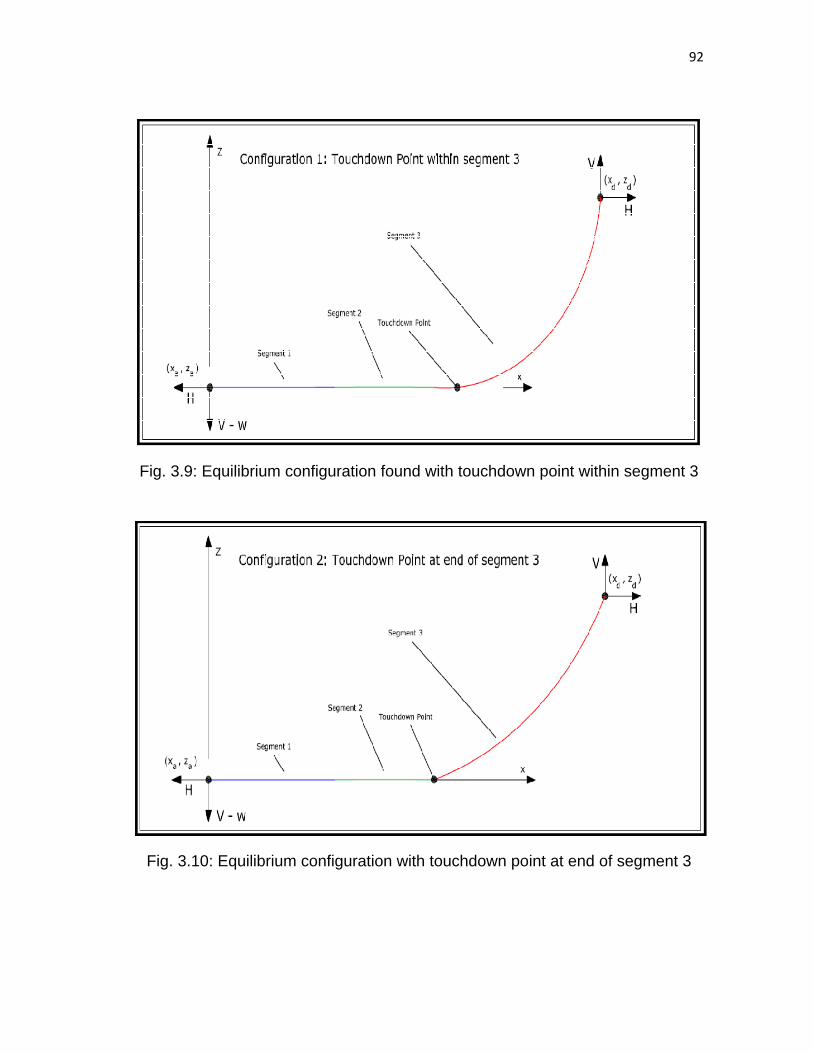
92
Fig. 3.9: Equilibrium configuration found with touchdown point within segment 3
Fig. 3.10: Equilibrium configuration with touchdown point at end of segment 3

93
Fig. 3.11: Equilibrium configuration found with touchdown point within segment 2
Fig. 3.12: Equilibrium configuration with touchdown point at end of segment 2
It is important to mention that figs. 3.9 to 3.14 are mildly exaggerated. For more
of the mooring line to be suspended, the floating vessel must move through
some offset distance. These figures are only directed at illustrating the

94
configuration of the mooring line when the touchdown point is at different
locations.
Fig. 3.13: Equilibrium configuration found with touchdown point within segment 1
Fig. 3.14: Equilibrium configuration with touchdown point at end of segment 1
Obtaining the restoring forces in the plane of each line is done with linear
interpolation. At this point, one may question the use of linear interpolation on a
curve that may in some cases be of a different (higher) order. In the formulation

95
of STAMOORSYS, one approach which was contemplated in an effort to
overcome this problem is the use of regression analysis on each resulting curve,
to obtain the equation relating plotted parameters. The challenge in using this
approach is to justify the order of the polynomial used in the regression analysis.
For a given resulting curve, if the variables are related by a polynomial of higher
degree than that used in the regression analysis, then the errors which will be
incurred will most likely be significant. A safer (i.e. one with lower possibility of
large errors) approach would be to assume the continuous curve to be a
piecewise continuous function. Discretizing the function into very small linear
functions validates linear interpolations between the end points of each small
segment. Although greater interpolation accuracy can be achieved by fitting a
polynomial through these very close points (especially along the steep section of
the restoring force versus departure curve), wrong interpolated values can be
obtained along the flat section of the curve as illustrated in fig. 3.15. It then
follows that the greater the number of small discrete linear functions, the greater
the accuracy of the interpolation process.
Fig. 3.15: Challenge in using higher order interpolation in STAMOORSYS
‐200‐100
0100200300400500600700800900
0 500 1000 1500 2000
Restoring Forces
Departures
Preliminary Restoring Forces versus Corresponding Departures
Preliminary Curve
Poly. (Preliminary Curve)

96
To ensure that the linear interpolation process yields accurate results, the error
between two values of restoring force obtained for the same departure by using
two sets of points is calculated. Figure 3.16 depicts the process of verifying the
accuracy of the interpolation. The first set of points ),( 11 yx and ),( 22 yx are used
to interpolate for 21−iy , with a known value of ix . This interpolation is repeated
using ),( 33 yx and ),( 44 yx with the same known ix to obtain 413−iy . The
percentage difference between 21−iy and
413−iy is computed; a difference of up to
5% indicates that interpolation is inaccurate, otherwise the value of 21−iy is
adopted as the interpolated restoring force corresponding to a departure of ix .
Fig. 3.16: Verification of linear interpolation accuracy
Once the restoring forces in the plane of each line have been obtained through
the interpolation process, the principles of statics are applied to resolve the

97
forces into their different components, and the global forces on the vessel are
then computed in each axis. For any arrangement of mooring lines (such as in
fig. 3.17), the horizontal global forces on the floating vessel can be computed
using eqns. (3.39) and (3.40).
Fig. 3.17: A 4-line mooring system with 0,0 >> offoff YX offset
∑ ∑=
=n
iiiX HF
1cosθ (3.39)
∑∑=
=n
iiiY HF
1
sinθ (3.40)
where 8,......2,1=n and ⎟⎠⎞⎜
⎝⎛= −
i
ii X
Y1tanθ after the vessel has moved to the new
offset position.
Each given offset produces corresponding global restoring forces on the vessel.
The global stiffness is a measure of the change in the global forces with respect
to distance (offset). Considering that the offsets specified by the user may not
always be in constant increments or reductions, computing the slopes (stiffness)
along the global restoring force versus offset curves requires a scheme that
handles unequal offsets effectively. Finite difference expressions presented in

98
Yang [29] are used in computing the global stiffness. The forward difference
formula is applied to the first point, and the backward difference formula is
applied to the last point. For intermediate points, the central difference
expression is used in computing the stiffness. Denoting the global stiffness by Kthe global stiffness in the horizontal axes can therefore be written as:
dxdF
K xx = (3.41)
dydF
K yy = (3.42)
For the first point on the x -axis curve, the forward difference expression is:
[ ] [ ] [ ])(
2
2121
2221
21 1121
xxxxFFxFFxxFFx
dxdF iiiiii xxxxxxx
Δ+ΔΔΔ
−Δ+−ΔΔ+−Δ= ++++ (3.43)
The central difference formula applied to intermediate points on the x -axis curve
is:
[ ] [ ])( 11
221 11
−−
−
Δ+ΔΔΔ
−Δ+−Δ= −+
iiii
xxixxix
xxxxFFxFFx
dxdF iiii (3.44)
The backward difference is computed on the x -axis curve using the formula:
[ ] [ ] [ ])(
2
9898
2998
28 1112
xxxxFFxFFxxFFx
dxdF iiiiii xxxxxxx
Δ+ΔΔΔ
−Δ+−ΔΔ+−Δ= −−−− (3.45)
Equations (3.43) to (3.45) are similarly applied to the y -axis curves to compute
the stiffness along the y -axis. In case the reader is pondering why the subscripts
in the backward difference expression are “8” and “9”, STAMOORSYS plots the
global restoring force versus offset curves using a total of 10 points, which

99
implies a total of 9 segments between the points. The 8th and 9th segments are
used in computing the backward difference for the stiffness at the 10th point.
3.3 A DESCRIPTION OF THE FEATURES IN STAMOORSYS
There are six sheets or pages in STAMOORSYS, and these are:
• Problem Set-Up Page
• Line Response Plot Page
• Restoring Forces Plot Page
• Design Page
• Calculations Page
• Bank Page
PROBLEM SET-UP PAGE
The problem set-up page is the first page to be used in STAMOORSYS for any
project. It holds input values of mooring line properties and coordinates of
anchors and fairleads. The page also holds the known offsets for which the
static responses of the mooring system will be investigated. Only information for
the number of lines to be used is required; so for a 4-line analysis only inputs for
four lines are needed.
Unacceptable entries into STAMOORSYS will return error messages prompting
the user of the acceptable range or formats of inputs. An instance is when the
input of an offset is a negative number. The error prompt shown in fig. 3.18
pops-up to inform the user of the acceptable inputs.

100
Fig. 3.18: STAMOORSYS offset error prompt
Some other discrepancies may lead to unusual run times, where the simulation
just keeps running as though it will never come to an end. In such situations, the
user may cancel the run using the escape key on the computer key pad, and
check through the inputs for inconsistent entries.
The code execution buttons are arranged in the order of usage during the
analysis. Seven (7) code execution controls are available to the user in the set-
up page, and these are shown on fig. 3.19. Amongst all seven controls, the last
three (‘Reset’, ‘Clear Inputs’, and ‘Clear Outputs’) implement tasks which are
less computational compared to the first four controls (‘Run Statics’, ‘Global
Forces’, ‘Update Lines 1 to 4’ and ‘Update Lines 5 to 8’).
A vital component to note is the ‘Check!’ related to the computed departures and
preliminary departures (shown under the code execution buttons). After running
statics (by clicking ‘Run Statics’) this check must read ‘Range is ok’ before
further analysis is continued. Otherwise, the check cell will read ‘Extend Range’.

101
Fig. 3.19: Tasks executed by different user controls in set-up page
Read-in anchor, fairlead and offset
coordinates.
Compute departures in the plane of the line
and display on set-up page.
Read-in line properties and
preliminary range of forces.
Compute preliminary
departures using equilibrium
equations, and display on
calculations page.
Read computed restoring forces in the plane of the
line, (from calculations page) and display on set-
up page.
Read global restoring forces from calculations page and display on set-up page.
Read line properties and
restoring forces in the plane of lines 1
to 4 from set-up page.
Compute tensions at fairleads and
anchors, suspended lengths, and
lengths on seafloor for lines1 to 4 and display on set-up
page.
Read line properties and
restoring forces in the plane of lines 5
to 8 from set-up page.
Compute tensions at fairleads and
anchors, suspended lengths, and
lengths on seafloor for lines 5 to 8 and display on set-up
page.
Delete all values of preliminary
restoring forces and computed
preliminary departures from
calculations page.
Delete all input values on set-up
page.
Delete all output values on set-up
page, except check for satisfactory
range of departures.

102
Table 3.2: Display of check related to preliminary and computed departures
Table 3.3: Sample display of check related to grid resolution
The ‘Extend Range’ feedback suggests that the limits of the preliminary restoring
forces (in the input section) must be extended. In Table 3.2, the quantities
labeled “A” are the minimum and maximum values of the departures computed
for all lines used in analysis. That is, all the given offsets have been applied to
the lines used in the design simulation and their respective departures are
computed. The lowest departure amongst all the lines considering all given
offsets displays as the “Min. Departure”, while the maximum departure of all the
computed departures displays as the “Max. Departure”. On the other hand, the
set of quantities labeled “B” in Table 3.2 are the minimum and maximum values
of all the departures computed from the preliminary range of restoring forces
specified by the user. Each restoring force is used in computing a departure; and
so for the number of points specified by the user, a set of restoring forces and
departures is produced. STAMOORSYS then finds the minimum departure
computed using the preliminary restoring forces and displays it as “Min. Prel.
Departure” while it displays the maximum value computed as “Max. Prel.
Departure”.
A
B

103
An additional check to confirm the adequacy of grid (distance between two
points along the preliminary restoring force versus preliminary departure curve)
resolution is performed by STAMOORSYS. As shown in Table 3.3, if the grid
resolution is adequate the program displays “0” for the number of points with
%5≥ error. Otherwise, the number of points for which the interpolation error is
%5≥ is reported. If the designer so wishes, the resolution can be increased or
reduced by adjusting the value for “number of points” and / or “maximum value
of force” in the preliminary range of restoring forces. A full view of the
STAMOORSYS problem set-up page can be found in appendix A1 of this
document.
LINE RESPONSE PLOTS PAGE
On this page, the static response plots from analysis performed in the problem
set-up page are shown. In other words, the static responses on this page will
only change automatically when analysis is performed in the problem set-up
page. The graphs displayed are suspended line lengths versus departures,
lengths of line on sea floor versus departures, tensions at anchor versus
departures, and tensions at fairlead versus departures for all lines (1 to 8). Only
the plots corresponding to the number of lines for which analysis is performed
will be automatically updated.
RESTORING FORCES PAGE
Here the restoring forces in all the lines are plotted against the departures of the
lines in their respective planes. These plots are tied to the set-up page only, and
as such will only be updated when analysis is performed on the set-up page.
Being able to view the plots in the presented array makes it fairly easy to
compare the restoring forces in each line. If a symmetric arrangement of
mooring lines is used in analysis, similar characteristics should be seen in plots

104
of corresponding mooring lines separated by the axis of symmetry. With the
arrangement of the restoring force plots, any inconsistencies in the plots can be
readily observed by the designer.
DESIGN PAGE
In the design page, only the input variables to be varied in the design process
are shown. Other input variables such as the vertical distance from fairlead to
seabed, coordinates of fairleads, inclination angles and offsets will be pulled
from the set-up page while the code is executing. It is therefore necessary to
ensure that these input variables are entered adequately in the set-up page to
represent the system undergoing design. The primary statics results of interest
(global restoring forces and global stiffness), computed departures and the
fairlead tensions in all the lines are shown on the same page. Again, the code
execution buttons are arranged in the order of analysis. As in the set-up page,
after running statics (by clicking ‘Run Statics’) the check related to the
departures must read ‘Range is ok’ before further analysis is continued.
Otherwise, the check cell will read ‘Extend Range’. The ‘Extend Range’
feedback suggests that the limits of the preliminary restoring forces (in the input
section) must be extended.
As can be observed in fig. 3.20, the design page is only one user control short
compared to the problem set-up page. While striving toward ensuring an efficient
design process, it is important that the user controls to be clicked while
performing the design is kept at the minimum possible. Unlike in the set-up
page, the global restoring forces are computed by the ‘Run Statics’ control in the
design page. Having two separate controls to update statics for the first four
lines and the last four lines could be an advantage if the designer is working with
four mooring lines or less. This essentially takes away the simulation / run time
that would be consumed if all eight lines were used in design.

105
An additional capability of the design page is to accept and incorporate the
target plots of global restoring forces which the designer intends to match as
closely as possible. Being able to visually compare equivalent design results
with the target (design) outputs from the prototype system is a necessary
capability that informs the designer of the proximity of the equivalent mooring
system’s trend of response to that of the target system. The most appreciable
fact about the STAMOORSYS design page is that it is self-contained, such that
the designer stays within the same page until the optimally designed statically
equivalent mooring system is achieved. Appendix A2 shows the design page.
It is worthy of mention that STAMOORSYS can also be used to determine static
horizontal force versus offset curves for prototype mooring systems, if such
systems satisfy the constraints embedded in STAMOORSYS (i.e. maximum of
eight lines, identical lines with maximum of three segments, equal fairlead
elevations and equal anchor depths).
CALCULATIONS PAGE
The calculations page contains raw intermediate results kept within the
spreadsheet to relieve the macro codes of some of the burden in the code
execution process. Given that the user controls which are hosted by Visual
Basic macros in Microsoft Excel have limits to the capacity of procedures
(codes) they can execute, there is greater potential of the software ‘crashing’ or
often getting ‘stuck’ in a ‘not responding’ mode if the codes embedded are right
around the limits of their capacity. Therefore performing some of the
computations in the calculations page both reduces the risk of crashing the
program, and the computation time required by the macros.
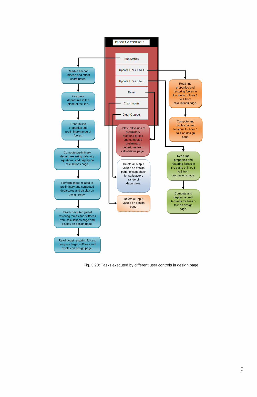
106
Fig. 3.20: Tasks executed by different user controls in design page
Read line properties and
restoring forces in the plane of lines 1
to 4 from calculations page.
Compute and display fairlead
tensions for lines 1 to 4 on design
page.
Read-in anchor, fairlead and offset
coordinates.
Compute departures in the plane of the line.
Read-in line properties and
preliminary range of forces.
Compute preliminary departures using catenary equations, and display on
calculations page.
Read line properties and
restoring forces in the plane of lines 5
to 8 from calculations page.
Compute and display fairlead
tensions for lines 5 to 8 on design
page.
Delete all values of preliminary
restoring forces and computed
preliminary departures from
calculations page.
Delete all input values on design
page.
Delete all output values on design
page, except check for satisfactory
range of departures. Perform check related to
preliminary and computed departures and display on
design page.
Read computed global restoring forces and stiffness from calculations page and
display on design page.
Read target restoring forces, compute target stiffness and
display on design page.

107
The user does not require any activity in the calculations page. This page only
interfaces with the design and problem set-up pages as necessary. No
interactive interface exists therein, even though the arrangements of the
computation cells are such that the designer / user understands their contents. It
is recommended though, that the user makes no attempt to effect any changes
in the calculations page, as this may disrupt a routine in STAMOORSYS. The
spreadsheet cells in the calculations page contain a lot of formulae, any of which
if deleted will adversely affect the working of the program.
BANK PAGE
Within the bank page calculations are performed and computed results are sent
to the ‘calculations’ page. Like the calculations page, no user interface exists in
the bank page. The major computations performed are the interpolations to
assess the adequacy of the grid resolution used in analysis. Again, performing
these calculations in the spreadsheet is intended to reduce the amount of code
to be executed by user controls in STAMOORSYS.
A summarized recommended approach to the use of STAMOORSYS is given in
fig. 3.21.
Fig. 3.21: Summary of recommended approach in the use of STAMOORSYS
The additional usefulness of the Set-up, Line Response and Restoring Forces
pages is that they make the debugging process for STAMOORSYS a lot easier
and they provide additional detailed information for comparison with other codes.
Enter required data in problem
set-up page.
Enter required data in problem
design page.
Design statically
equivalent mooring
Return to problem set-up page and run statics using the satisfactory
design inputs to obtain full results and plots.

108
Being able to visualize line configurations for each line used in the simulation
offers a good opportunity to verify that the results portray static behaviors that
are physically correct.

109
CHAPTER IV
APPLICATION OF STAMOORSYS IN DESIGN OF STATICALLY EQUIVALENT MOORING SYSTEMS
4.1 ANALYSIS OF SINGLE LINE MOORING SYSTEMS USING
STAMOORSYS, Orcaflex AND LINANL
Although the major purpose for STAMOORSYS is the design of statically
equivalent spread mooring systems, it is important to demonstrate first that the
software analyzes single line mooring systems with acceptable accuracy since
the underlying principles used in analyzing spread mooring systems are
essentially those of single line systems. LINANL is a static mooring analysis
program with the capability of handling multi-component lines. This section
discusses three hypothetical cases which are analyzed using STAMOORSYS
and LINANL, and one realistic case using Orcaflex, STAMOORSYS and
LINANL.
Fig. 4.1: Problem set-up for single line analysis using STAMOORSYS, Orcaflex and LINANL A floating structure is moored using a 3-segment mooring line as shown in fig.
4.1, with the line properties shown in Table 4.1 for each case of analysis. The

110
task is to compute the departure of the vessel, under specified values of
restoring forces. Tensions at the anchor and fairlead, suspended lengths and
lengths on the sea floor computed for each given restoring force are also
obtained from both programs and compared. Recalling that the process of
computing the departure in STAMOORSYS is numerical, the value of the
computed fairlead elevation at convergence (for each applied force) is also
obtained and compared to actual fairlead elevation. At least for STAMOORSYS,
this comparison (actual versus computed fairlead elevations) in a sense
measures the accuracy of the numerical computations. Each test case is a result
of varying one or more properties (length, axial stiffness, weight per unit length)
of the mooring line. In the first three test cases the fairlead elevation is
maintained at a value of 1500 ft above the anchor.
The vessel is subjected to ten different restoring forces ranging from 20000 Ibs
to 200,000 Ibs at increaments of 20,000 Ibs. Figures 4.2 through 4.6 show the
comparison between STAMOORSYS and LINANL for the first case.
Fig. 4.2: Restoring forces versus departures for Case 1
0
50000
100000
150000
200000
250000
1500.00 1600.00 1700.00 1800.00 1900.00 2000.00
Restoring Forces (lbs)
Departures (ft)
Restoring Forces vs DeparturesCase 1
STAMOORSYS
LINANL

111
Table 4.1: Mooring line properties for hypothetical problem
Segment No. Length (ft) EA (Ibs) Weight per unit length (Ibs/ft)
CASE 1
1 1000 21E010
800
2 1000 21E010
800
3 1000 21E010
800
CASE 2
1 1000 21E010
800
2 550 21E010
800
3 650 21E010
800
CASE 3
1 1000 21E010
800
2 550 205E09
700
3 650 21E010
800
Tables 4.2, 4.3 and 4.4 show the results for the three test cases, respectively.
For each case percentage differences between the outputs from LINANL and
STAMOORSYS are computed. These differences are very small, indicating a
strong agreement between both programs.
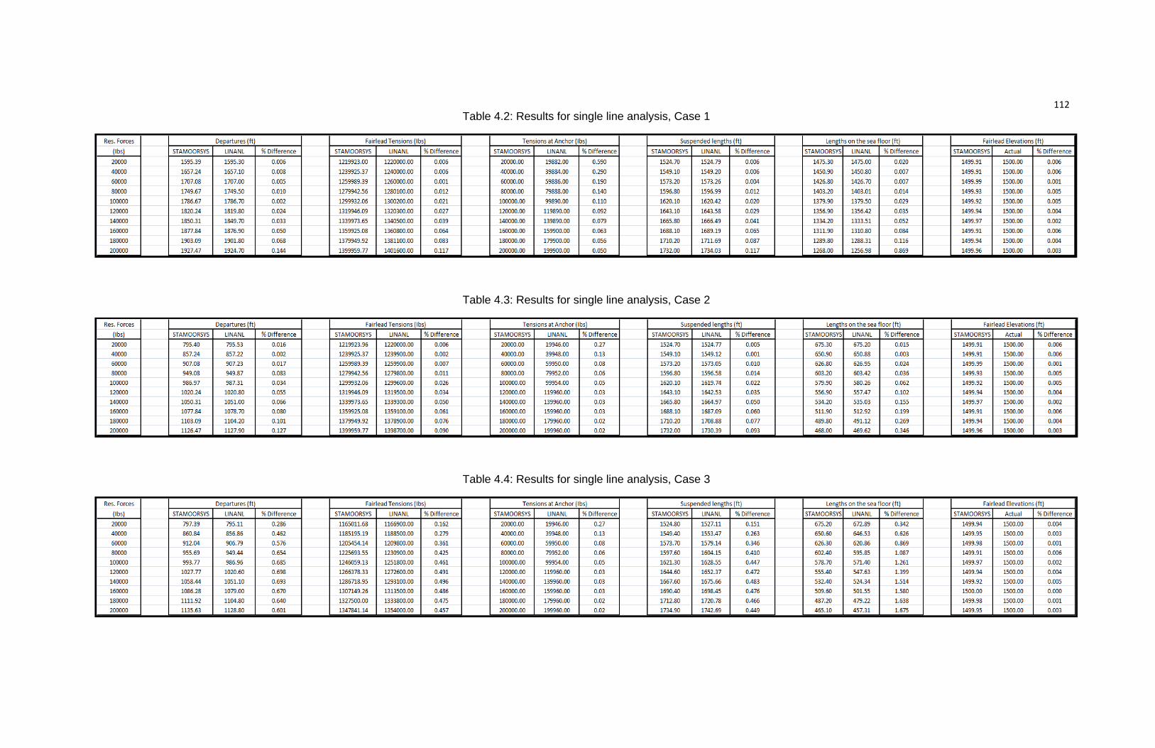
112
Table 4.2: Results for single line analysis, Case 1
Table 4.3: Results for single line analysis, Case 2
Table 4.4: Results for single line analysis, Case 3

113
Fig. 4.3: Restoring forces versus fairlead tensions for Case 1
Fig. 4.4: Restoring forces versus tensions at the anchor for Case 1
0
50000
100000
150000
200000
250000
1200000 1250000 1300000 1350000 1400000 1450000
Restoring Forces (Ibs)
Tensions at Fairlead (Ibs)
Restoring Forces vs Fairlead TensionsCase 1
STAMOORSYS
LINANL
0
50000
100000
150000
200000
250000
0 50000 100000 150000 200000 250000
Restoring Forces (Ibs)
Tensions at Anchor (Ibs)
Restoring Forces vs Tensions at AnchorCase 1
STAMOORSYS
LINANL
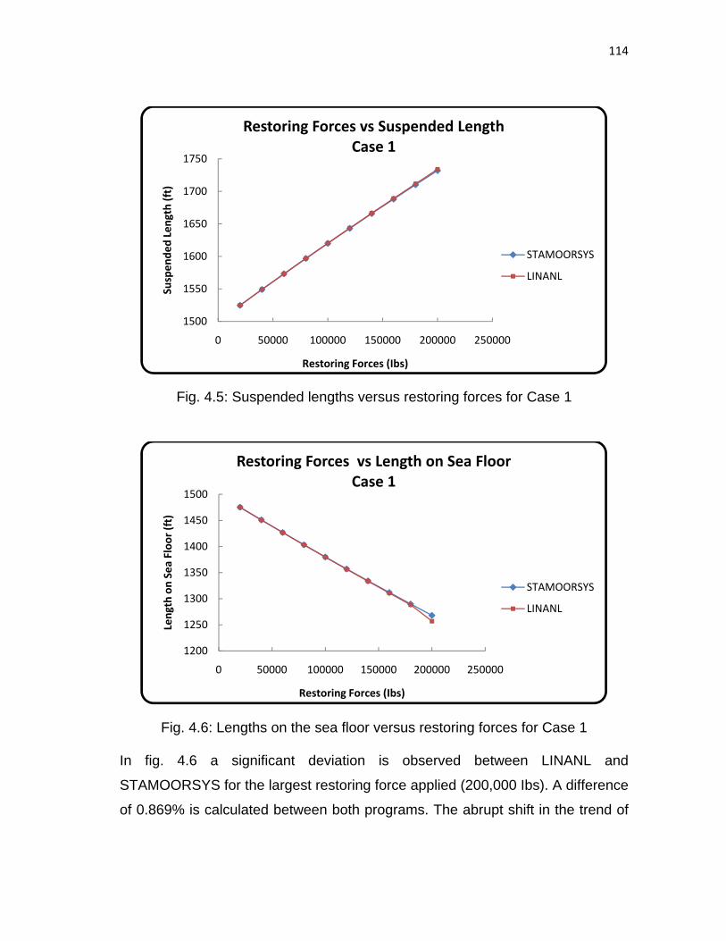
114
Fig. 4.5: Suspended lengths versus restoring forces for Case 1
Fig. 4.6: Lengths on the sea floor versus restoring forces for Case 1
In fig. 4.6 a significant deviation is observed between LINANL and
STAMOORSYS for the largest restoring force applied (200,000 Ibs). A difference
of 0.869% is calculated between both programs. The abrupt shift in the trend of
1500
1550
1600
1650
1700
1750
0 50000 100000 150000 200000 250000
Suspen
ded Length (ft)
Restoring Forces (Ibs)
Restoring Forces vs Suspended LengthCase 1
STAMOORSYS
LINANL
1200
1250
1300
1350
1400
1450
1500
0 50000 100000 150000 200000 250000
Length on Sea Floo
r (ft)
Restoring Forces (Ibs)
Restoring Forces vs Length on Sea FloorCase 1
STAMOORSYS
LINANL

115
the LINANL curve suggests that the value computed for the force of 200,000 Ibs
is not indicative of equilibrium. Perhaps the iterative process in LINANL reached
convergence with some significant error. It is important to mention that LINANL
is coded to reach numerical convergence when the difference between the
actual and computed fairlead elevations is within a specified error limit (such as
≤ 5% of the actual fairlead elevation). Unfortunately, the user has no opportunity
to select a convenient error limit for analysis while making inputs to LINANL.
However, the differences in computed departures and tensions for both
programs are very small.
Comparisons made between both programs for the second case are depicted in
figs. 4.7 through 4.11. Computed departures, tensions and line configurations at
equilibrium agree very strongly. The suspended lengths and lengths on sea floor
computed by both programs show the results to be physically correct.
Fig. 4.7: Restoring forces versus departures for Case 2
0
50000
100000
150000
200000
250000
750 850 950 1050 1150
Restoring Forces (Ibs)
Departures (ft)
Restoring Forces vs DeparturesCase 2
STAMOORSYS
LINANL

116
Fig. 4.8: Restoring forces versus fairlead tensions for Case 2
Fig. 4.9: Restoring forces versus tensions at the anchor for Case 2
0
50000
100000
150000
200000
250000
1200000 1250000 1300000 1350000 1400000 1450000
Restoring Forces (Ibs)
Tensions at Fairlead (Ibs)
Restoring Forces vs Fairlaed TensionsCase 2
STAMOORSYS
LINANL
0
50000
100000
150000
200000
250000
0 50000 100000 150000 200000 250000
Restoring Forces (Ibs)
Tensions at Anchor (Ibs)
Restoring Forces vs Tensions at AnchorCase 2
STAMOORSYS
LINANL

117
Fig. 4.10: Suspended lengths versus restoring forces for Case 2
Fig. 4.11: Lengths on the sea floor versus restoring forces for Case 2
1500
1550
1600
1650
1700
1750
0 50000 100000 150000 200000 250000
Suspen
ded Length (ft)
Restoring Forces (Ibs)
Restoring Forces vs Suspended LengthCase 2
STAMOORSYS
LINANL
0
100
200
300
400
500
600
700
800
0 50000 100000 150000 200000 250000
Length on Sea Floo
r (ft)
Restoring Forces (Ibs)
Restoring Forces vs Length on Sea FloorCase 2
STAMOORSYS
LINANL
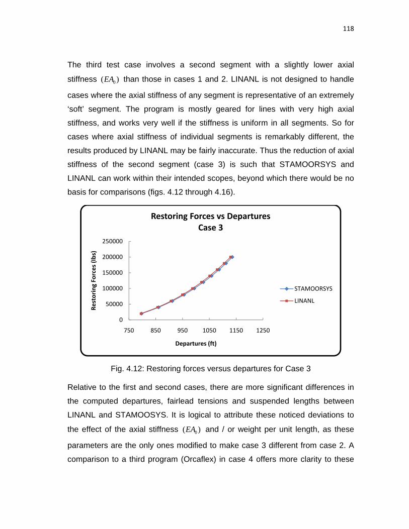
118
The third test case involves a second segment with a slightly lower axial
stiffness )( 0EA than those in cases 1 and 2. LINANL is not designed to handle
cases where the axial stiffness of any segment is representative of an extremely
‘soft’ segment. The program is mostly geared for lines with very high axial
stiffness, and works very well if the stiffness is uniform in all segments. So for
cases where axial stiffness of individual segments is remarkably different, the
results produced by LINANL may be fairly inaccurate. Thus the reduction of axial
stiffness of the second segment (case 3) is such that STAMOORSYS and
LINANL can work within their intended scopes, beyond which there would be no
basis for comparisons (figs. 4.12 through 4.16).
Fig. 4.12: Restoring forces versus departures for Case 3
Relative to the first and second cases, there are more significant differences in
the computed departures, fairlead tensions and suspended lengths between
LINANL and STAMOOSYS. It is logical to attribute these noticed deviations to
the effect of the axial stiffness )( 0EA and / or weight per unit length, as these
parameters are the only ones modified to make case 3 different from case 2. A
comparison to a third program (Orcaflex) in case 4 offers more clarity to these
0
50000
100000
150000
200000
250000
750 850 950 1050 1150 1250
Restoring Forces (Ibs)
Departures (ft)
Restoring Forces vs DeparturesCase 3
STAMOORSYS
LINANL

119
deviations. It is important to establish STAMOORSYS’ capability to produce
correct results for mooring lines with low axial stiffness )( 0EA .
Fig. 4.13: Restoring forces versus fairlead tensions for Case 3
Fig. 4.14: Restoring forces versus tensions at the anchor for Case 3
0
50000
100000
150000
200000
250000
1150000 1200000 1250000 1300000 1350000 1400000
Restoring Forces (Ibs)
Tensions at Fairlead (Ibs)
Restoring Forces vs Fairlaed TensionsCase 3
STAMOORSYS
LINANL
0
50000
100000
150000
200000
250000
0 50000 100000 150000 200000 250000
Restoring Forces (Ibs)
Tensions at Anchor (Ibs)
Restoring Forces vs Tensions at AnchorCase 3
STAMOORSYS
LINANL

120
Fig. 4.15: Suspended lengths versus restoring forces for Case 3
Fig. 4.16: Lengths on the sea floor versus restoring forces for Case 3
1500
1550
1600
1650
1700
1750
1800
0 50000 100000 150000 200000 250000
Suspen
ded Length (ft)
Restoring Forces (Ibs)
Restoring Forces vs Suspended LengthCase 3
STAMOORSYS
LINANL
0
100
200
300
400
500
600
700
800
0 50000 100000 150000 200000 250000
Length on Sea Floo
r (ft)
Restoring Forces (Ibs)
Restoring Forces vs Length on Sea FloorCase 3
STAMOORSYS
LINANL

121
In general the comparisons between STAMOORSYS and LINANL for the first
three cases are very close. Overall, the differences in computed values may be
attributed to computational errors during numerical iterations. With the reason
that the accuracy of the iterative solutions could be improved by the user in
STAMOORSYS but not in LINANL, it is logical to suggest that the tolerance limit
in LINANL is such that the iterative procedure does not converge with accurate
values when large forces are applied to a line with relatively low axial stiffness.
A fourth case used in validating STAMOORSYS is considered, where a system
is moored by a single line in a model test wave basin. The properties of the
mooring system components are realistic for model test purposes (design of
equivalent mooring systems). Table 4.5 summarizes the properties of the
system components. Restoring forces used in analysis range from a minimum of
47500 Ibs to a maximum of 2,892,400 Ibs.
Table 4.5: Properties of mooring system components for test Case 4
SEGMENT
)(0 IbsEA )/( ftIbsw )( ftL
Fairlead Elevation
)( ft
1 1.89E09 25 1684.7
1015.80
2 3.87E06 3042 201
3
1.88E09 4135.40 15
Using these values, single line analyses are performed with STAMOORSYS,
LINANL and Orcaflex. One may ponder the non-use of Orcaflex in the validation
test cases 1, 2 and 3 previously discussed. The availability of the program for
this purpose is very limited as the only available license in the OTRC is shared
by engineers working on design verification projects. Coupled with this fact, it is
not so trivial to obtain local results from Orcaflex as it with LINANL. Knowledge

122
of how to use the software is required, and harvesting local results takes a
relatively longer time compared to LINANL.
Single line analyses using the inputs in Table 4.5 produced the results displayed
in figs. 4.17 and 4.18. The computed departures from all three programs fairly
follow the same trend, over the range of restoring forces considered. The
maximum percentage difference in departures computed using STAMOORSYS
and Orcaflex is 0.36%. Between STAMOORSYS and LINANL, the maximum
percentage difference is 1.70%. A significant deviation in computed departures
is observed between LINANL and both STAMOORSYS and Orcaflex.
Fig. 4.17: Restoring forces versus departures for Case 4
Similar to fig. 4.6 in case 1, the deviation corresponds to the maximum force
applied. For this force, Orcaflex and STAMOORSYS are in much stronger
agreement. All three programs compute suspended lengths of 1900.7 ft (the
0.00E+00
5.00E+05
1.00E+06
1.50E+06
2.00E+06
2.50E+06
3.00E+06
3.50E+06
1450.00 1550.00 1650.00 1750.00 1850.00
Restoring Forces (Ibs)
Departures (ft)
Restoring Forces versus Departures
Orcaflex
LINANL
STAMOORSYS

123
total length of the line) for all restoring forces applied. The departures obtained
from all three programs are plotted against the fairlead tensions associated with
them, in fig. 4.18. A more consistent agreement is exists between
STAMOORSYS and Orcaflex, than it does between LINANL and the other two
programs. The curves suggest that STAMOORSYS is capable of producing
correct results even for low axial stiffness ( 0EA ) and weights per unit length.
Fig. 4.18: Fairlead tensions versus departures for Case 4
Fairlead tensions computed by LINANL are slightly higher than those computed
by STAMOORSYS and Orcaflex, and this deviation tends to increase as the
departures (hence the forces) increase.
0.00E+00
5.00E+05
1.00E+06
1.50E+06
2.00E+06
2.50E+06
3.00E+06
3.50E+06
4.00E+06
4.50E+06
1450.00 1550.00 1650.00 1750.00 1850.00
Fairlead
Ten
sion
s (Ibs)
Departures (ft)
Fairlead Tensions versus Departures
Orcaflex
LINANL
STAMOORSYS

124
4.2 VALIDATION OF STAMOORSYS FOR STATIC GLOBAL ANALYSIS OF
SPREAD MOORING SYSTEMS
Considering that the design of statically equivalent mooring systems ultimately
leads to a comparison of results of static global analyses, it is necessary to
validate STAMOORSYS using known results in this regard before an actual
design case. This section discusses two validation cases, one of which is an
example problem presented in Jones [5], where a spread mooring system is
analyzed using MOORANL to obtain the horizontal global restoring forces on the
floating vessel. MOORANL is a FORTRAN program for analysis of spread
mooring systems. This example problem is repeated using STAMOORSYS and
the results are compared. The second validation case is a comparison between
STAMOORSYS and Orcaflex using equivalent mooring design results for a
representative model floater. Using the unique combination of mooring system
properties that led to a match (between prototype and equivalent) in the static
global restoring force versus offset and global stiffness versus offset curves in
Orcaflex, an effort is made to achieve the same match in STAMOORSYS.
First, consider a floating vessel with fairlead and anchor coordinates relative to
the center of the floater as presented in Table 4.6. The floater is moored using
four identical mooring lines. As presented in the example problem, each of the
four lines is a single segment line with length of 1700 ft, uniform weight per unit
length of 0.078 Ibs / ft, and uniform axial stiffness ( 0EA ) of 200,000 Ibs. The
length of 1700 ft is mimicked in STAMOORSYS (because it handles only three-
segment lines) as 200 ft of segment 1, 500 ft of segment 2 and 1000 ft of
segment 3. The fairlead elevation relative to the sea bed / anchor point is 400 ft.
For all three segments the same weights per unit length and axial stiffness as in
MOORANL are input in STAMOORSYS to represent lines of uniform properties.

125
Table 4.6: Fairlead and anchor coordinates for example problem
LINE
FAIRLEAD COORDINATES ANCHOR COORDINATES
X Y X Y
1 50.00 75.00 1183.99 1208.99
2 ‐50.00 75.00 ‐1183.99 1208.99
3 ‐50.00 ‐75.00 ‐1183.99 ‐1208.99
4 50.00 ‐75.00 1183.99 ‐1208.99
Five horizontal offsets are applied to the vessel at a 45o heading to make the
most loaded line in the system, line 3. The offsets range from 10 ft to 50 ft at
increments of 10 ft. These data are entered in STAMOORSYS as inputs and a
numerical value of 0.01 is used in the iterations. A preliminary range of restoring
forces from 0 to 800 Ibs, with 50 points for the preliminary restoring force versus
departure curve is used in analysis. The results from the example problem
produced using MOORANL are input into STAMOORSYS as the target curves
to be matched (as would be done for a target / prototype mooring system).
Fig. 4.19: MOORANL and STAMOORSYS x-axis global restoring force curves
‐450.00
‐400.00
‐350.00
‐300.00
‐250.00
‐200.00
‐150.00
‐100.00
‐50.00
0.00
0 10 20 30 40
Globa
l Restoring
Forces in x‐axis (Ibs)
Offsets in x‐direction (ft)
STAMOORSYS and MOORANL Fx Versus x‐axis Offsets
STAMOORSYS
MOORANL

126
Both MOORANL and STAMOORSYS compute the same global restoring forces
in the x and y directions as shown in figs 4.19 through 4. 22; this is no surprise
since the mooring system is symmetric about the center of the floater and the
offsets are applied on a 45o heading. The maximum percentage difference
between both programs is 4.1% for the global restoring forces.
Fig. 4.20: MOORANL and STAMOORSYS y-axis global restoring force curves
Fig. 4.21: MOORANL and STAMOORSYS x-axis global stiffness curves
‐450.00
‐400.00
‐350.00
‐300.00
‐250.00
‐200.00
‐150.00
‐100.00
‐50.00
0.00
0 10 20 30 40
Globa
l Restoring
Forces in y‐axis (Ibs)
Offsets in y‐direction (ft)
STAMOORSYS and MOORANL Fy Versus y‐axis Offsets
STAMOORSYS
MOORANL
0
5
10
15
20
25
30
35
0 10 20 30 40Globa
l Stiffne
ss in
X‐Direction
(Ibs/ft)
Offsets in X‐Direction (ft)
STAMOORSYS and MOORANL Kx Versus x‐axis Offsets
STAMOORSYS
MOORANL

127
For the global stiffness the maximum difference is 7.39%. The magnitudes of
these differences are relatively low and these results suggest a good agreement
between both programs, thereby validating STAMOORSYS.
Fig. 4.22: MOORANL and STAMOORSYS y-axis global stiffness curves
Consider the second validation case where the properties of the mooring system
components as used in Orcaflex are presented in Tables 4.7 and 4.8. Offset
increments range from 0.10 to 242.82 ft in the x-direction only. The actual
fairlead elevation relative to the anchor position is 1015.8 ft for all lines. Four
lines are used in the analysis and all lines are identical. The input data is entered
in STAMOORSYS and a ‘numerical increment value in iteration’ of 0.01 is used
in running statics. A minimum preliminary restoring force of 0 and a maximum of
3,500,000 Ibs are used with 500 points for the computation of the preliminary
restoring force versus departure curve. Regarding the target plots from Orcaflex
0
5
10
15
20
25
30
35
0 10 20 30 40
Globa
l Stiffne
ss in
Y‐Direction
(Ibs/ft)
Offsets in Y‐Direction (ft)
STAMOORSYS and MOORANL Ky Versus y‐axis Offsets
STAMOORSYS
MOORANL

128
to be the curves to be matched, these plots are entered into STAMOORSYS for
comparison.
Table 4.7: Mooring line properties for global analysis validation using Orcaflex
SEGMENT
0EA w L
1
1.89E09 25.87 1684.7
2 3.87E06 3042.00 201
3
1.88E09 4135.40 15
Table 4.8: Mooring line coordinates for global analysis validation using Orcaflex
LINE
FAIRLEAD
COORDINATES (ft)
ANCHOR
COORDINATES (ft)
X Y
X
Y
1 43.84 43.84 1210.57 1210.57
2 -43.84 43.84 -1210.57 1210.57
3 -43.84 -43.84 -1210.57 -1210.57
4 43.84 -43.84 1210.57 -1210.57

129
Fig. 4.23: Orcaflex and STAMOORSYS x-direction global restoring force curves
Fig. 4.24: Orcaflex and STAMOORSYS x-direction global stiffness curves
‐6000000.00
‐5000000.00
‐4000000.00
‐3000000.00
‐2000000.00
‐1000000.00
0.00
0.00 50.00 100.00 150.00 200.00 250.00 300.00
Globa
l Restoring
Forces in x‐axis (Ibs)
Offsets in x‐direction (ft)
STAMOORSYS and Orcaflex Fx Versus X‐Direction Offsets
STAMOORSYS
Orcaflex
0
5000
10000
15000
20000
25000
0.00 50.00 100.00 150.00 200.00 250.00 300.00
Globa
l Stiffne
ss in
X‐Direction
(Ibs/ft)
Offsets in X‐Direction (ft)
STAMOORSYS and Orcaflex Kx Versus X‐Direction Offsets
STAMOORSYS
Orcaflex

130
In comparing the global restoring forces (fig. 4.23) a maximum difference of
5.46% is computed while a maximum difference of 5.23% is computed for global
stiffness (fig. 4.24). It is fair to infer that these differences are relatively low, and
suggest a good agreement in the global static forces and stiffness in the mooring
system between STAMOORSYS and Orcaflex.
To emphasize the importance of a high resolution (fine grid points) in the design
of statically equivalent mooring systems, the global analysis verification exercise
between STAMOORSYS and Orcaflex is repeated with 100 points used in
computing the preliminary restoring force versus departure curve. Using a lower
resolution (coarser grid points) the maximum percentage difference in global
stiffness between STAMOORSYS and Orcaflex increases to 5.46%. Keeping the
resolution high may incur more computation time, but it is certainly a good
strategy that enhances the designer’s search for a match in the static global
response curves.
Considering the difference in the solution approach between Orcaflex and
STAMOORSYS, there is bound to be some differences in the computed
solutions. Orcaflex uses a numerical discrete element approach, where each
element is treated as a lump mass. STAMOORSYS on the other hand is based
on analytical solutions to the catenary equations. This fundamental difference in
computation procedures suggests that there will always be differences in the
obtained results, though these differences cannot be enormous if both programs
apply their respective solution methods correctly.
4.3 DESIGN OF STATICALLY EQUIVALENT DEEPWATER MOORING
SYSTEM
Armed with the approach discussed in the third chapter of this work, the goal in
this section is to discuss a typical design case for a statically equivalent mooring
system performed using STAMOORSYS. The basic information provided for

131
design includes the target global restoring force and stiffness curves obtained
from the design of the prototype mooring system. These curves are computed
over a specified range of offsets, and must be matched with tolerable errors by
the equivalent mooring design over the same range of offsets. Engineering
properties of the line segments of the prototype mooring system are also known,
and these are considered in making good first guesses for the properties of the
statically equivalent mooring system.
The prototype mooring is a 3x3 system (3 groups of 3 lines each) arranged
symmetrically about the horizontal x-axis and with all lines identical. Each line
consists of a 350 ft long upper platform chain segment followed by a 5940 ft long
polyester rope segment followed by a 500 ft long lower anchor chain segment.
The platform chain and anchor chain are both 4-1/4” chains with submerged
weight of 132.2 lb/ft and axial stiffness of 235,319 kips. The polyester rope has
submerged weight of 4.5 lb/ft and axial stiffness of 48,500 kips. The vertical
distance from the seafloor to the fairleads is 4310 ft. Relative to the vertical axis
of the spar, the fairlead radius is 46.02 ft and the anchor radius is 5328.5 ft. A
plan view sketch of the prototype mooring system is shown in fig. 4.25.
Fig. 4.25: Plan view sketch of prototype mooring system

132
The global coordinate system is located on the vertical axis of the spar and
oriented such that the negative horizontal x-axis lines up with the central
mooring line in one of the 3 groups. The spar will be tested with one weather
environment only, one where the positive x-axis points down-weather.
Therefore only the positive x-axis excursions of the spar are of interest in this
design problem. Considering that the mooring arrangement is not symmetric
about the horizontal y-axis, the force versus offset curve (for x-direction offsets)
is not symmetric about zero offset. The target restoring force versus offset curve
that is supposed to be matched is set up in STAMOORSYS for positive x-axis
offset values associated with negative horizontal restoring forces.
Fig. 4.26: Plan view sketch of equivalent mooring set-up
The objective is to design a 3-line equivalent mooring system (as shown in fig.
4.26) that matches the horizontal force versus offset curve and the horizontal
stiffness versus offset curve of the prototype mooring with the following
tolerances:

133
• Over the horizontal offset range from 15.56 ft to 251.50 ft, the global
horizontal restoring force curve for the equivalent mooring should match
that of the prototype to within 5%
• Over the horizontal offset range from 15.56 ft to 251.50 ft, the global
horizontal stiffness curve for the equivalent mooring should match that of
the prototype to within 10%.
The model of the spar will be built with the fairleads at the same location as the
prototype, and so the fairlead coordinates (x, y) in feet for lines 1, 2 and 3 will be
(-46.02, 0.00), (23.01, 39.85) and (23.01, -39.85) respectively. Since the model
will be tested in the OTRC basin, the vertical distance from the fairleads to the
basin floor will be 495 ft and the anchor radius must not exceed 1,440 ft. Each
line will consist of a load (tension cell) attached to the fairlead, followed by a coil
spring and a length of stainless steel cable. In full scale units, the load cell will
have a length of 13.125 ft, a submerged weight of 747 lb/ft and an axial stiffness
of 700,000 kips. The steel cable will have a submerged weight of 346.12 lb/ft
and an axial stiffness of 705,957 kips.
In order to design the statically equivalent mooring system it will be necessary to
select values for:
• the length of the stainless steel cable attached between the anchor and
the coil spring
• the length, submerged weight and axial stiffness of the coil spring
• the anchor locations.
The parameters of the equivalent mooring which are varied during the design
process are the coordinates of the anchors relative to the center of the platform,
the lengths of the line segments, the axial stiffness and submerged unit weight

134
of the coil spring. The preliminary range of restoring forces is also adjusted to
increase the grid resolution during analysis.
To highlight some significant points, two design solutions are provided to this
problem; one which has features which can be criticized and another which may
be regarded as fully acceptable. For the first design solution provided,
comparisons of global restoring force versus offset curves between the
prototype and the statically equivalent mooring system are shown in figs 4.27
and 4.28. For the range of offsets considered, the maximum percentage
difference in the computed global restoring forces between the prototype
mooring system and the statically equivalent mooring system along the x-axis is
4.80%. The global stiffness curves of the prototype and equivalent systems
differed by a maximum of 10.0%.
Fig. 4.27: Equivalent and prototype global restoring forces for design solution 1
‐4.50E+06
‐4.00E+06
‐3.50E+06
‐3.00E+06
‐2.50E+06
‐2.00E+06
‐1.50E+06
‐1.00E+06
‐5.00E+05
0.00E+00
0.00 100.00 200.00 300.00
Globa
l Restoring
Forces in x‐axis (Ibs)
Offsets in x‐direction (ft)
Equivalent and Prototype Fx Versus X‐Direction Offsets
Equivalent
Prototype

135
Fig. 4.28: Equivalent and prototype global stiffness for design solution 1
A summary of the properties of the designed statically equivalent system is
given in Table 4.9. The solution consists of a symmetric arrangement of
anchors about the horizontal x-axis, and this is required to ensure that under the
action of a static force along the x-direction the vessel does not offset in the y-
direction. The selected axial stiffness is within an acceptable range and the
length of 700 ft can be achieved by connecting springs in series. However, a
spring with submerged weight as low as 50 Ibs/ft, cannot both produce the
design stiffness and support the associated tensions in the line. Such springs
are not commercially available, so this raises the issue of designing a system
that theoretically satisfies the requirements but cannot actually be built.
6000
8000
10000
12000
14000
16000
18000
0.00 100.00 200.00 300.00
Globa
l Stiffne
ss in
X‐Direction
(Ibs/ft)
Offsets in X‐Direction (ft)
Equivalent and Prototype Kx Versus X‐Direction Offsets
Equivalent
Prototype

136
Table 4.9: Properties of first equivalent mooring design solution
SEGMENT
0EA (Ibs)
w (Ibs/ft)
L (ft)
LINE Anchor Coordinates
x (ft) y (ft)
1 7.06E08 346.12 255 1 -1192.0 0.00
2 6.52E06 50 700 2 774.0 791.50
3
7.00E08 747.00 13.13 3 774.0 -791.50
Given that a numerical process is involved in the design simulations, it is
important to emphasize that the accuracy of the design directly relates to the
accuracy of both the numerical simulations and the adequacy of the grid
resolution used. The design solution in Table 4.6 was obtained with a ‘numerical
increment value in iteration’ of 0.1 and 100 grid points. On repeating the
simulations using the same design results but with a numerical increment value
of 0.01, the maximum difference in the global stiffness curves increased to
13.16% which is higher than the allowable value of 10.0%; this is unacceptable.
This observation suggests the relevance of high accuracy in the numerical
simulations. No alarming difference is observed with the number of grid points
increased to 200. One may expect that with the very close match in the global
restoring force versus offset curves (fig 4.27), a match between the stiffness
curves is almost guaranteed for all offsets. The post processing done with the
outputs of the first design solution suggests otherwise. Obtaining matching
curves for the global restoring force and stiffness involves independent
observation of both curves during the design process. It is easy to assume that
because both curves often and inextricably respond to changes made to the
properties of the mooring system, matching one within the required tolerance will
automatically guarantee that the second will be satisfied as well. The reality
however, is that the designer could still face a significant challenge in matching

137
say the stiffness curves within the specified tolerance, even when the global
restoring curves have been matched to much lower than the required tolerance
limit for all offsets in the specified range.
A more acceptable design solution is presented in Table 4.10. This second
design still has the anchor positions symmetric about the horizontal x-axis.
Compared to the first design solution, the second solution has a heavier and
shorter coil spring that is slightly lower in axial stiffness, for the middle segment.
The weight of the coil spring is such that at it can resist the tensions in the
mooring line and conveniently produce the design stiffness. Overall, this system
is buildable in the OTRC wave basin.
Table 4.10: Properties of second equivalent mooring design solution
SEGMENT
0EA (Ibs)
w (Ibs/ft)
L (ft)
LINE Anchor Coordinates
x (ft) y (ft)
1 7.06E08 346.12 788.00 1 -1120.02 0.00
2 4.35E06 1374.26 294.94 2 560.01 969.97
3
7.00E08 747.00 13.13 3 560.01 -969.97
Compared to the global restoring forces and stiffness curves obtained in the first
solution, those of the second solution are quite similar but with slight noticeable
differences. The maximum percentage difference in global restoring forces
between the prototype and equivalent systems is 4.86%. The maximum
difference in the global stiffness curves is 6.29%. Figures 4.29 and 4.30 show
the global restoring force and stiffness curves respectively.

138
Fig. 4.29: Equivalent and prototype global restoring forces for design solution 2
Fig. 4.30: Equivalent and prototype global stiffness for design solution 2
‐4.50E+06
‐4.00E+06
‐3.50E+06
‐3.00E+06
‐2.50E+06
‐2.00E+06
‐1.50E+06
‐1.00E+06
‐5.00E+05
0.00E+00
0.00 100.00 200.00 300.00
Globa
l Restoring
Forces in x‐axis (Ibs)
Offsets in x-direction (ft)
Equivalent and Prototype Fx Versus X‐Direction Offsets
Equivalent
Prototype
0
2000
4000
6000
8000
10000
12000
14000
16000
18000
20000
0.00 50.00 100.00 150.00 200.00 250.00 300.00
Globa
l Stiffne
ss in
X‐Direction
(Ibs/ft)
Offsets in X‐Direction (ft)
Equivalent and Prototype Kx Versus X‐Direction Offsets
Equivalent
Prototype

139
Considering the orders of magnitude of the computed percentage differences
between these curves, it is fair to infer that the second design for the equivalent
mooring system is sufficient for the spar testing project. The strong agreements
between the equivalent and prototype curves suggest a strong basis for the
comparison of dynamic responses obtained during model testing.
In practice, the designed equivalent system would be updated to compensate for
the difference between the design properties and the as-built properties and
adjustments in the wave basin. The updated design however does not differ
significantly from the preliminary design of the statically equivalent mooring
system.
The local results of static equilibrium for the second design solution are
computed using the Set-up page in STAMOORSYS. These results include
tensions at the anchors and fairleads, suspended line lengths, lengths of line on
the sea floor and local restoring forces. Appendix B shows the local results of
static equilibrium. The line configurations indicate that the system is a taut
mooring system as all the lines are suspended for each applied offset, except for
the last and largest offset at which about 3.5 ft of lines 2 and 3 is on the seafloor.

140
CHAPTER V
SUMMARY AND CONCLUSIONS
The importance of verifying designs of deepwater floating structures cannot be
overemphasized. Measuring static and dynamic responses of floating structures
during model testing offers proper insights on the behavior of the floater. This
research embraces the hybrid method of design verification, which combines
numerical simulations with model testing to reduce the level of uncertainties
associated with model testing. One of the challenges in testing model floaters in
the wave basin remains the spatial and depth limitations of wave tanks. For
deepwater systems, direct scaling of the prototype mooring systems is often not
possible and a mere truncation of the mooring system means that the moorings
in the wave basin cannot impose the same static loads on the model floater, as
the full depth moorings on the prototype structure. It is therefore necessary to
design a statically equivalent mooring system that will impose the same static
global loads on the model floater, as in the full depth system. To design this
system, an efficient numerical tool is required.
Having identified the need for a fit-for-purpose tool in the design of statically
equivalent mooring systems (which is a step in the hybrid verification process),
STAMOORSYS has been produced through this research to meet this need.
STAMOORSYS is a program for static analyses of spread mooring systems,
specifically tailored to be easily used in the design of statically equivalent
deepwater mooring systems. It accepts the properties of the mooring system
components and other spatial data (e.g. anchor coordinates) as inputs, and uses
these to statically analyze the mooring system for local and global responses
(departures, restoring forces, stiffness, tensions and line configurations at static
equilibrium). The program is geared for easy repetition of analyses in the effort
to design (optimize) a statically equivalent mooring system, and this is
achievable using the design page. For this reason the global restoring force and

141
global stiffness curves are provided in the design page, such that the designer
can instantly visualize the global effects of alterations made to the system during
design.
Without the consideration of certain factors from a realistic perspective, perhaps
it may not be very easy to appreciate the advantages of STAMOORSYS
regarding statically equivalent deep water mooring systems. Typical factors here
include requirements from clients (owners of floating structure to be tested in the
wave tank), time available to complete testing project, portability of the program
and the effort required of a new user to understand and use STAMOORSYS
compared to programs performing similar functions. Like many programs, the
version of STAMOORSYS produced at this stage of the research project has
some limitations, and these will also be discussed in this chapter.
5.1 ECONOMIC ADVANTAGES OF STAMOORSYS
As sponsor of this research project, the Offshore Technology Research Center
reserves the right to use of this program. From personal communications with
engineers (in the OTRC) involved with design verification processes such as that
described in the third chapter of this work, it is possible and often the case that
client requirements are stringent. The level of static equivalence to be achieved
may be one with very high accuracy. Allowable errors between the target curves
and those produced from the equivalent design is best kept at the minimum
possible, to preserve the integrity of the basis for comparing dynamic responses.
As STAMOORSYS is hosted in a Microsoft Excel spreadsheet, it is completely
trivial to format cells such that the results displayed are to very high precision.
STAMOORSYS offers both local and global results making comparisons easy
and offering complete insight on static mooring configurations resulting from the
given design properties of the system.

142
The current version of the program is only about 5938 KB in capacity, and thus
can easily be carried about in a portable memory drive or even saved on a
secure folder on a network to make it more readily accessible to the user(s).
STAMOORSYS requires no additional hardware such as dongles for
accessibility, and this is one less limitation.
Considering the fact that a new user (say, a new engineer on a project) may
require the use of STAMOORSYS on a verification project, one does not have to
worry so much about learning to use the program. The user interfaces in
STAMOORSYS are self explanatory, and it is easy to move through the different
pages of the program. Average knowledge of the use of Microsoft Excel would
be just about adequate for a user to optimally put STAMOORSYS to use. This
may not be so easy with other available programs performing similar or the
same tasks; usually special knowledge of the software is required and this may
take a while to grasp.
5.2 LIMITATIONS OF STAMOORSYS AND UP-COMING MODIFICATIONS
The current version of STAMOORSYS only addresses horizontal offsets and
horizontal restoring forces on a floating vessel. For some floating structures (e.g.
semi-submersibles) it is important to establish static equivalence in the vertical
direction (relating to heave motions) as well as in the rotating plane relating to
pitch motions of the floater. At a given offset location vertical restoring forces act
on the floater causing it to tilt unevenly. Usually, the tilt versus offset curve
experienced by the model floater in the wave basin comprises a steep slope
which is not likely to be observed in the prototype structure. The local moments
and vertical global restoring forces for the model floater must be compared to
the local moments and vertical restoring forces of the prototype structure. Such
capability should be added to the program to make it versatile enough to

143
address static equivalence in more directions of typical interest, for
representative structures that could be tested in the OTRC.
An additional constraint in the current version of STAMOORSYS is that all lines
attached to the vessel have the same fairlead and anchor elevations, and are of
the same composition ( 0EA , w and L ). Sometimes, it is not such a good idea to
make lines on the up-weather side of the floater have the same properties as
those on the down-weather side. It is desired to afford the user the opportunity to
create each line composition such that it is unique. With such capability the
optimization process is made more efficient, as the designer would have more
properties to modify in the search for a match between the compared curves.
Not having enough information on commercially available components of
mooring systems could lead to unbuildable designs, and eventually loss of time
as such designs must be repeated. A database of properties of vendor mooring
components (especially springs, cables and chains) could also be added to
STAMOORSYS to speed the convergence to a buildable design. This will
essentially point the designer(s) to the ranges of properties within which a
buildable design solution can be obtained.
The current version of STAMOORSYS requires a manual optimization of the
mooring system properties in search of a match in the global restoring force and
global stiffness curves. With the in-built capability of Microsoft Excel to solve
optimization problems, efforts will be made to enhance the optimization process
in STAMOORSYS, such that design process is highly facilitated. The challenge
in achieving this is handling the many design variables for the number of lines
used in analysis. Additionally, using the optimizer in Excel to control the iterative
computations in STAMOORSYS may not be very trivial. However, harnessing
Excel’s optimizer to enhance the design process is worth the effort considering
that its computation speed is very high; this can save a lot of time.

144
5.3 CONCLUSIONS
Using the hybrid method of design verification to verify the designs of deepwater
floating structures is greatly embraced by the industry. As exposed in the
discussed literature in the second chapter of this work, the processes of
modeling the model and designing a statically equivalent mooring system
require efficient numerical tools. This research has provided a tool which is
specifically tailored to perform one of the tasks required in the hybrid method.
STAMOORSYS has the capability of producing accurate results as shown in the
comparisons made in the fourth chapter of this work. It is also very
advantageous that the program offers the user a clear insight on the local effects
of the chosen properties, as displayed under parameters such suspended line
lengths and length of the line on the sea floor. Being able to control the
accuracies of the numerical simulations and grid resolutions is part of the
program’s strong capabilities. The interfaces of STAMOORSYS are created to
minimize distractions in the design process which may arise from switching
between windows and menus (as is the case in many other programs). Another
unique advantage is being able to use the tools inherently available in Microsoft
Excel, for any form of post processing which the designer / user may require.
The user may also choose to save the spreadsheet for archival purposes after a
particular project.
Although STAMOORSYS uses a numerical process in computing results of
static equilibrium, the search for static equilibrium is a deterministic process.
Many existing programs (especially finite element codes) use more approximate
procedures in obtaining results. One of such techniques is specifying the anchor
coordinates of the lines, and computing the coordinates of the top attachment
point with numerical simulations and vice versa. The challenge with this
procedure is that it is prone to inaccurate predictions of the touchdown point of

145
the mooring line. STAMOORSYS regards the touchdown point as a sensitive
parameter in the numerical process, and thus the computation of this parameter
is a lot more thorough than is obtainable in most other programs.
The major point of this research project has been to make life easier for the
designers of statically equivalent deepwater mooring systems, by developing a
tool specifically for this purpose. With the measure of achievement so far with
STAMOORSYS, it is fair to say that the goal has been achieved to some extent,
although more improvements (by eliminating the constraints discussed in section
5.2) to the program will make it even more useful.

146
REFERENCES
[1] Stansberg, C. T., Karlsen, S. I., Ward, E. G., Wichers, J. E. W. and Irani,
M. B., 2004, “Model Testing for Ultradeep Waters,” OTC Conference,
Houston, OTC 16587, pp. 1 - 8.
[2] Department of Marine Technology, Norwegian University of Science and
Technology, “Experimental Methods in Marine Hydrodynamics,” January
2008, http://www.ntnu.no/imt/research.
[3] McNatt, T. R., 1982, “Catenary Ocean Mooring Systems – Approaches to
Analysis and Testing,” IEEE Conference, 0197-7385/82/0000-0513, pp.
517 - 518.
[4] Jones, H. L., 1991, “Lecture notes on LINANL - Program for Static
Analysis of Mooring Systems,” Department of Civil Engineering, Texas
A&M University, College Station, TX.
[5] Jones, H. L., 1983, “MOORANL Users Guide - Program for Static
Analysis of Spread Mooring Systems,” Department of Civil Engineering,
Texas A&M University, College Station, TX, pp. 48 - 54.
[6] Orcina Limited, “Orcaflex Software,” version 9.1a, Cumbria, UK.
[7] Fernandez, J., 2008, “Reliability of Mooring Chains,” Proceedings of
TEKNA Conference on DP and Mooring of Floating Offshore Units,
Alesund, Norway.
[8] Richards, D., 2007, “Misrepresented Imports,” Proceedings of the 7th
International Rope Technology Workshop, College Station, TX.
[9] Wu, S., 2007, “Taut-leg Mooring and Anchoring for Spars,” Ocean
Engineering Seminar, Texas A&M University, College Station, TX.
[10] Kim, M. H., 2004, “Dynamic Analysis Tool for Moored Tanker-Based
FPSO’s Including Large Yaw Motions,” Final Report Prepared for the
Minerals Management Service under the MMS/OTRC Cooperate
Research Agreement, http://www.mms.gov, pp. 2 - 4.

147
[11] Luo, Y., Baudic, S., Poranski, P., Ormberg, H., Stansberg, C. T. and
Wichers, J., 2004, “Prediction of FPSO Responses: Model Tests versus
Numerical Analysis,” OTC Conference, Houston, OTC 16585, pp. 1 - 7.
[12] Stansberg, C. T., Ormberg, H. and Oritsland, O., 2002, “Challenges in
Deep Water Experiments: Hybrid Approach,” Transactions of the ASME,
124, pp. 90 - 95.
[13] Fylling, I. J. and Stansberg, C. T., 2005, “Model Testing of Deepwater
Floating Production Systems: Strategy for Truncation of Moorings and
Risers,” Proceedings of 17th DOT Conference, Vitoria, Brazil, pp. 1 - 4.
[14] Ormberg, H., Stansberg, C. T., Yttervik, R. and Kleiven, G., 1999,
“Integrated Vessel Motion and Mooring Analysis Applied in Hybrid Model
Testing,” Proceedings of the 9th ISOPE Conference, Brest, France, I, pp.
339 - 346.
[15] ITTC Specialist Committee on Deep Water Mooring, 1999, “Report from
the Specialist Committee on Deep Water Mooring,” 22nd ITTC
Proceedings, Seoul, Korea & Shanghai, China, II, pp. 377 - 398.
[16] Smith R. J. and MacFarlane, C. J., 2001, “Statics of a Three Component
Mooring Line,” Ocean Engineering, 28(7), pp. 899 – 914.
[17] Carbono, A. J., Menezes, I. F. M. and Martha, L. F., 2005, “Mooring
Pattern Optimization using Genetic Algorithms,” 6th World Congress of
Structural and Multidisciplinary Optimization, Rio de Janeiro, Brazil, pp. 1
- 9.
[18] Connaire A., Kavanagh K., and Ahilan R. V., 1999, “Integrated Mooring
and Riser Design - Analysis Methodology,” OTC Conference, Houston,
OTC 10810, pp. 1 - 11.
[19] Russell J. C. and Lardner T. J., 1997, “Statics Experiments on an Elastic
Catenary,” Journal of Engineering Mechanics, 123(12), pp. 1322 - 1324.
[20] Irvine, H. M., 1975, “Statics of Suspended Cables,” J. Engrg. Mech. Div.,
ASCE, 101(30), pp. 187 - 205.

148
[21] Irvine, H. M. and Sinclair, G. B., 1976, “The Suspended Elastic Cable
Under the Action of Concentrated Vertical Loads”, J. Solids Struct., 12,
pp. 309 - 317.
[22] Francois, M., 2005, “Fiber Ropes for Station-keeping: Engineering
Properties and Qualification Procedures,” IEEE Conference, 2, pp. 1623 -
1629.
[23] Banfield S. J., Casey, N. F., Nataraja, R., 2005, “Durability of polyester
deepwater mooring rope,” OTC Conference, Houston, I, OTC 17510, pp.
1 - 9.
[24] François, M., Davies, P., 2000, “Fibre rope deep water mooring: a
practical model for the analysis of polyester mooring systems,” Rio
Offshore Oil and Gas Conference, IBP 247 00.
[25] Bureau Veritas, 1997, “Certification of Synthetic Fiber Ropes for Mooring
Systems,” Bureau Veritas Certification Guidance Notes, NI 432 DTO
R00E.
[26] Casey, N. F. and Banfield, S. J., 2005, “Factors Affecting the
Measurement of Axial Stiffness of Polyester Deepwater Mooring Rope
Under Sinusoidal Loading,” OTC Conference, Houston, OTC 17068, pp. 1
- 11.
[27] Bowden G., 2004, “Stretched Wire Mechanics,” work supported by
Department of Energy, Geneva, pp. 1 - 8.
[28] Irvine, H. M., 1981, “Cable Structures,” MIT Press, Cambridge, MA, pp. 1-
24.
[29] Yang, W., 2007, “Hydrodynamic Analysis of Mooring Lines Based on
Optical Tracking Experiments,” PhD dissertation in Ocean Engineering,
Texas A&M University, College Station, TX, pp. 48 – 49.

149
APPENDIX A

150
Appendix A1: Set-up Page in STAMOORSYS
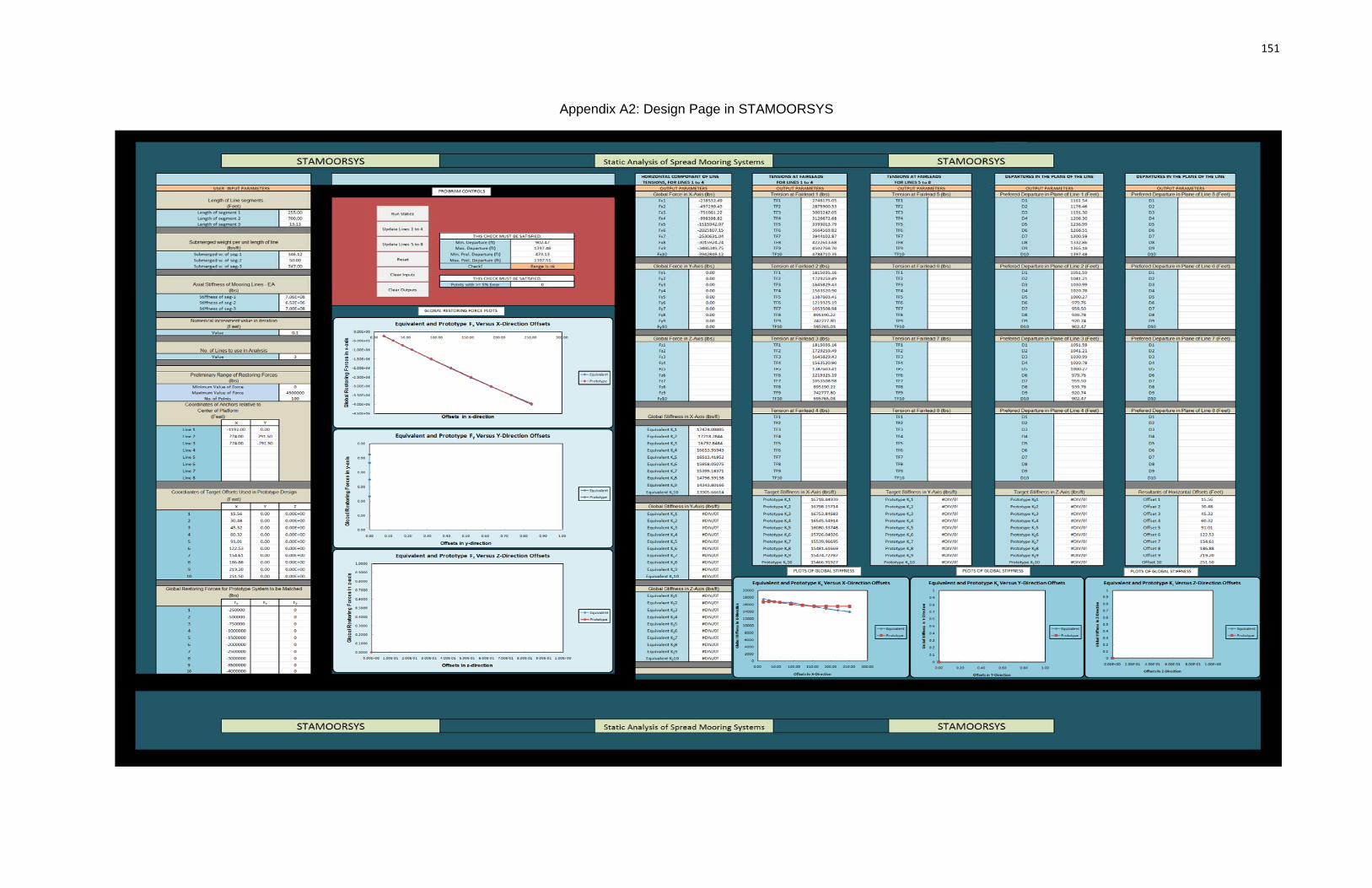
151
Appendix A2: Design Page in STAMOORSYS

152
APPENDIX B

153
Appendix B1: LOCAL RESULTS FOR LINE 1
0.00
200.00
400.00
600.00
800.00
1000.00
1200.00
1000.00 1100.00 1200.00 1300.00 1400.00
Suspen
ded Length (ft)
Departure (ft)
Suspended Length vs Departure
0.00
0.10
0.20
0.30
0.40
0.50
0.60
0.70
0.80
0.90
1.00
1000.00 1100.00 1200.00 1300.00 1400.00
Length on Seafloor (ft)
Departure (ft)
Length on Seafloor vs Departure
0.00
500000.00
1000000.00
1500000.00
2000000.00
2500000.00
3000000.00
3500000.00
4000000.00
4500000.00
5000000.00
1000.00 1100.00 1200.00 1300.00 1400.00
Tension at Ancho
r (Ibs)
Departure (ft)
Tension at Anchor vs Departure
0.00
1000000.00
2000000.00
3000000.00
4000000.00
5000000.00
6000000.00
1000.00 1100.00 1200.00 1300.00 1400.00
Tension at Fairlead (Ibs)
Departure (ft)
Tension at Fairlead vs Departure
0.00
500000.00
1000000.00
1500000.00
2000000.00
2500000.00
3000000.00
3500000.00
4000000.00
4500000.00
5000000.00
1000.00 1100.00 1200.00 1300.00 1400.00
Restoring Force (Ibs)
Departure (ft)
Restoring Force in Line 1 vs Departure in Line 1

154
Appendix B2: LOCAL RESULTS FOR LINE 2
1092.00
1092.50
1093.00
1093.50
1094.00
1094.50
1095.00
1095.50
1096.00
1096.50
950.00 1000.00 1050.00 1100.00
Suspen
ded Length (ft)
Departure (ft)
Suspended Length vs Departure
0.00
0.50
1.00
1.50
2.00
2.50
3.00
3.50
4.00
950.00 1000.00 1050.00 1100.00
Length on Seafloor (ft)
Departure (ft)
Length on Seafloor vs Departure
0.00
200000.00
400000.00
600000.00
800000.00
1000000.00
1200000.00
950.00 1000.00 1050.00 1100.00
Tension at Ancho
r (Ibs)
Departure (ft)
Tension at Anchor vs Departure
0.00
200000.00
400000.00
600000.00
800000.00
1000000.00
1200000.00
1400000.00
1600000.00
950.00 1000.00 1050.00 1100.00
Tension at Fairlead (Ibs)
Departure (ft)
Tension at Fairlead vs Departure
0.00
200000.00
400000.00
600000.00
800000.00
1000000.00
1200000.00
950.00 1000.00 1050.00 1100.00
Restoring Force (Ibs)
Departure (ft)
Restoring Force in Line 2 vs Departure in Line 2

155
Appendix B3: LOCAL RESULTS FOR LINE 3
1092.00
1092.50
1093.00
1093.50
1094.00
1094.50
1095.00
1095.50
1096.00
1096.50
950.00 1000.00 1050.00 1100.00
Suspen
ded Length (ft)
Departure (ft)
Suspended Length vs Departure
0.00
0.50
1.00
1.50
2.00
2.50
3.00
3.50
4.00
960.00 980.00 1000.00 1020.00 1040.00 1060.00 1080.00
Length on Seafloor (ft)
Departure (ft)
Length on Seafloor vs Departure
0.00
200000.00
400000.00
600000.00
800000.00
1000000.00
1200000.00
950.00 1000.00 1050.00 1100.00
Tension at Ancho
r (Ibs)
Departure (ft)
Tension at Anchor vs Departure
0.00
200000.00
400000.00
600000.00
800000.00
1000000.00
1200000.00
1400000.00
1600000.00
950.00 1000.00 1050.00 1100.00
Tension at Fairlead (Ibs)
Departure (ft)
Tension at Fairlead vs Departure
0.00
200000.00
400000.00
600000.00
800000.00
1000000.00
1200000.00
950.00 1000.00 1050.00 1100.00
Restoring Force (Ibs)
Departure (ft)
Restoring Force in Line 3 vs Departure in Line 3

156
VITA
IKPOTO ENEFIOK UDOH
Research Assistant, Offshore Technology Research Center
Coastal and Ocean Engineering, Texas A&M University
3136 TAMU, Texas 77843-3136
USA
EDUCATION
M.S., Ocean Engineering, Texas A&M University, 2008
B.Eng., Civil and Environmental Engineering, University of Port Harcourt, 2004
RECOGNITIONS / AWARDS
D. Michael Hughes Scholarship Award, Ocean Engineering Program, Texas
A&M University, 2007.
Akwa Ibom State Scholarship Award, Nigeria, 2006.
Federal Government Scholarship Award, Nigeria, 2002.
PROFESSIONAL MEMBERSHIPS AND LEADERSHIP POSITIONS HELD
President, Offshore Technology Research Center Graduate Students Forum
(OTRCGSF), Texas A&M University, USA (2007 – Present)
Current Member, American Society of Civil Engineers (ASCE)
General Parade Commander, National Youth Service Corps (NYSC), Zamfara
State, Nigeria (2005 – 2006)