Embed Size (px)
DESCRIPTION
Development of Defect Assessment Methods for Pipelines – Part 1 Integrity Group Lunch and Learn 1 Tom Bubenik July 19, 2007 © Det Norske Veritas AS. All rights reserved Slide 201August2007 Corrosion Defects – Types and Characteristics External Metal Loss (Corrosion) 2 © Det Norske Veritas AS. All rights reserved Slide 401August2007
Citation preview
1
Development of Defect Assessment Methods for Pipelines – Part 1
Integrity Group Lunch and Learn
Tom BubenikJuly 19, 2007
© Det Norske Veritas AS. All rights reserved Slide 201 August 2007
Outline
Corrosion Defects – Types and Characteristics
Analysis Methods for Corrosion
Analysis Methods for Cracks (Part 1)
2
Corrosion Defects – Types and Characteristics
© Det Norske Veritas AS. All rights reserved Slide 401 August 2007
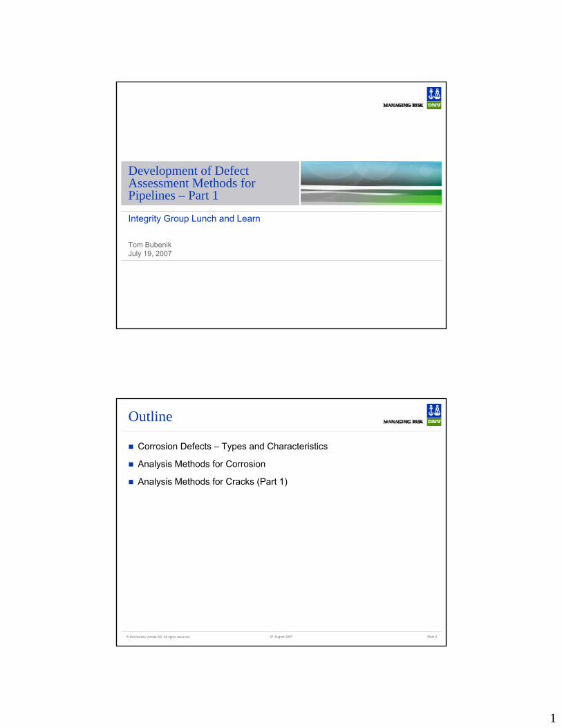
Groove or Narrow Axially Aligned Corrosion
Preferential Corrosion
Complex areas of Interacting pits;
general corrosion
Isolated pitting
External Metal Loss (Corrosion)
3
© Det Norske Veritas AS. All rights reserved Slide 501 August 2007
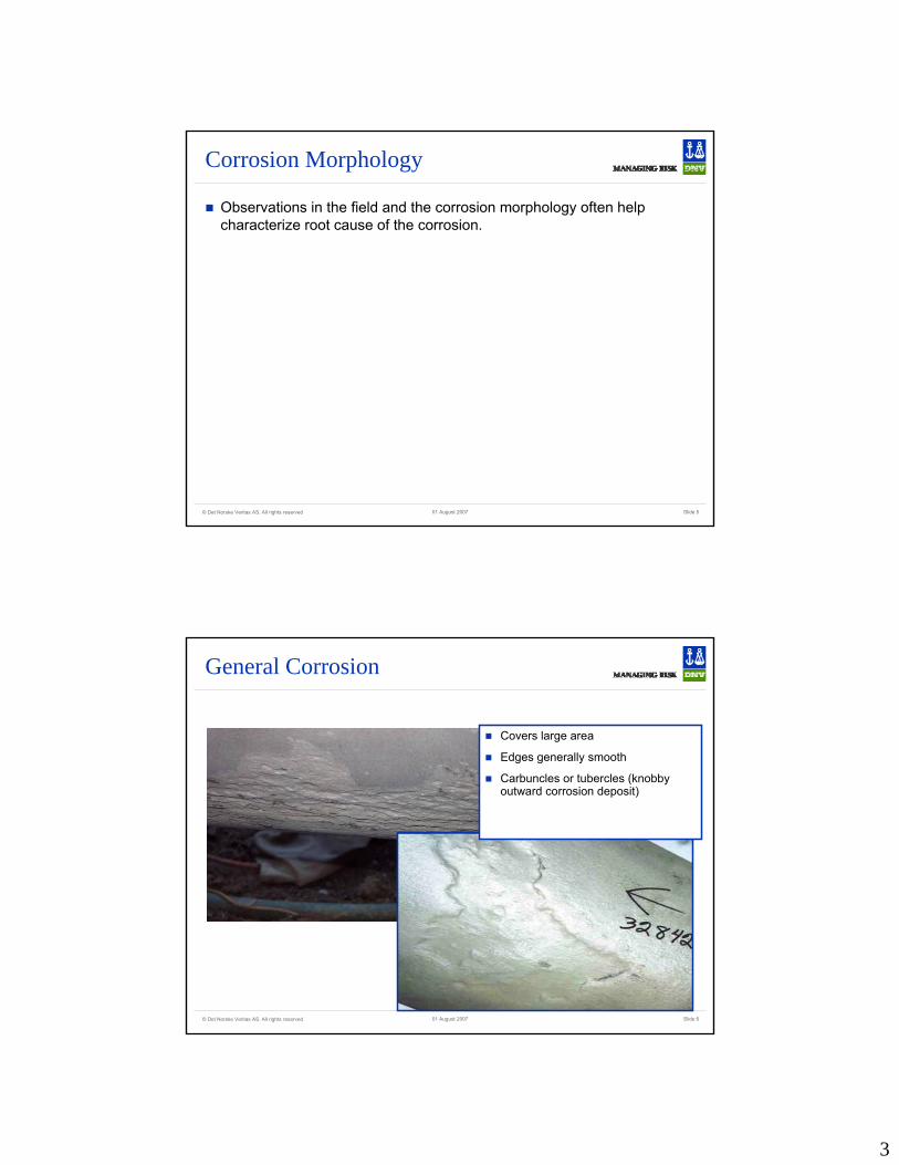
Corrosion Morphology
Observations in the field and the corrosion morphology often help characterize root cause of the corrosion.
© Det Norske Veritas AS. All rights reserved Slide 601 August 2007
General Corrosion
Covers large area
Edges generally smooth
Carbuncles or tubercles (knobby outward corrosion deposit)
4
© Det Norske Veritas AS. All rights reserved Slide 701 August 2007
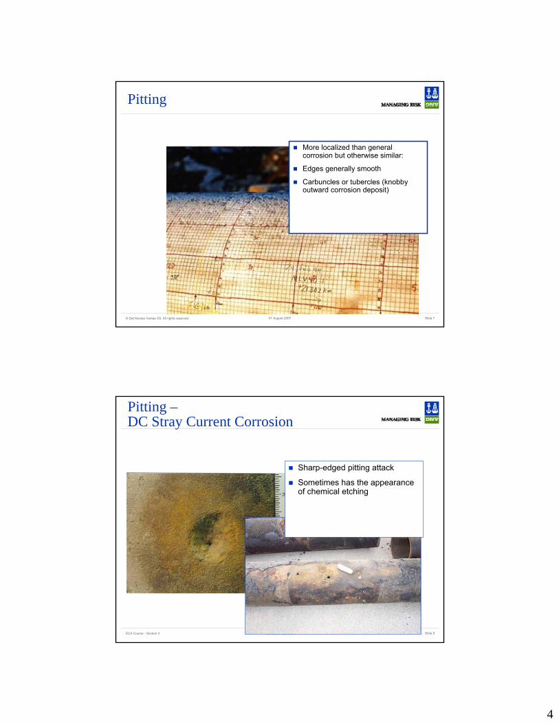
Pitting
More localized than general corrosion but otherwise similar:
Edges generally smooth
Carbuncles or tubercles (knobby outward corrosion deposit)
ECA Course - Section 3 Slide 8January 21-22, 2004
Pitting –DC Stray Current Corrosion
Sharp-edged pitting attack
Sometimes has the appearance of chemical etching
5
ECA Course - Section 3 Slide 9January 21-22, 2004
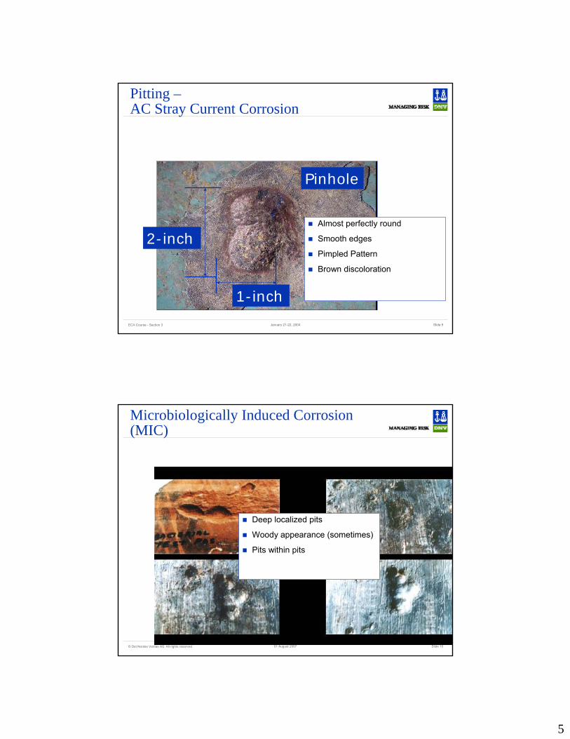
Pitting –AC Stray Current Corrosion
1-inch
2-inch
Pinhole
Almost perfectly round
Smooth edges
Pimpled Pattern
Brown discoloration
© Det Norske Veritas AS. All rights reserved Slide 1001 August 2007
Microbiologically Induced Corrosion (MIC)
Deep localized pits
Woody appearance (sometimes)
Pits within pits
6
© Det Norske Veritas AS. All rights reserved Slide 1101 August 2007
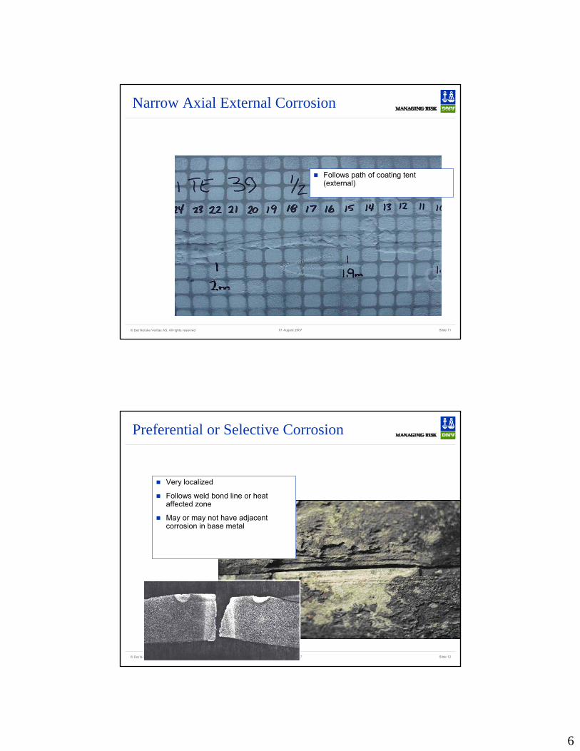
Narrow Axial External Corrosion
Follows path of coating tent (external)
© Det Norske Veritas AS. All rights reserved Slide 1201 August 2007
Preferential or Selective Corrosion
Very localized
Follows weld bond line or heat affected zone
May or may not have adjacent corrosion in base metal
7
© Det Norske Veritas AS. All rights reserved Slide 1301 August 2007
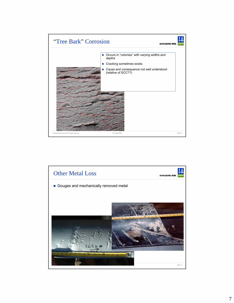
“Tree Bark” Corrosion
Occurs in “colonies” with varying widths and depths
Cracking sometimes exists
Cause and consequence not well understood (relative of SCC??)
© Det Norske Veritas AS. All rights reserved Slide 1401 August 2007
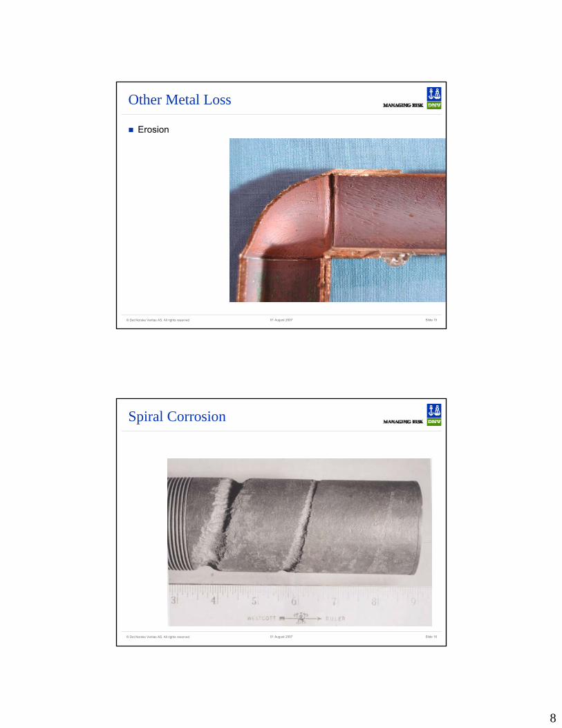
Other Metal Loss
Gouges and mechanically removed metal
8
© Det Norske Veritas AS. All rights reserved Slide 1501 August 2007
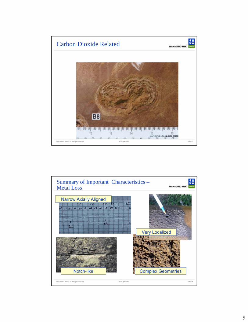
Other Metal Loss
Erosion
© Det Norske Veritas AS. All rights reserved Slide 1601 August 2007
Spiral Corrosion
9
© Det Norske Veritas AS. All rights reserved Slide 1701 August 2007
Carbon Dioxide Related
© Det Norske Veritas AS. All rights reserved Slide 1801 August 2007
Summary of Important Characteristics –Metal Loss
Narrow Axially Aligned
Notch-like Complex Geometries
Very Localized
10
Analysis Methods for Corrosion
Most Metal Loss is Analyzed Using ASME B31G or RSTRENG
Both are based on an analysis equation developed in the late 1960s and early 1970s
- B31G was originally referenced in Appendix G of the B31 Code.- RSTRENG is an acronym for the Remaining Strength of Corroded Pipe- Prior to development, the approach was to the degrade pressure carrying
capacity by the percent wall loss- The equation accounts for load shedding around shorter defects and it is
semi-empirical (includes analytic expression that accounts for stressconcentration due to bulging)
The same basic approach is accepted many places worldwide
11
© Det Norske Veritas AS. All rights reserved Slide 2101 August 2007
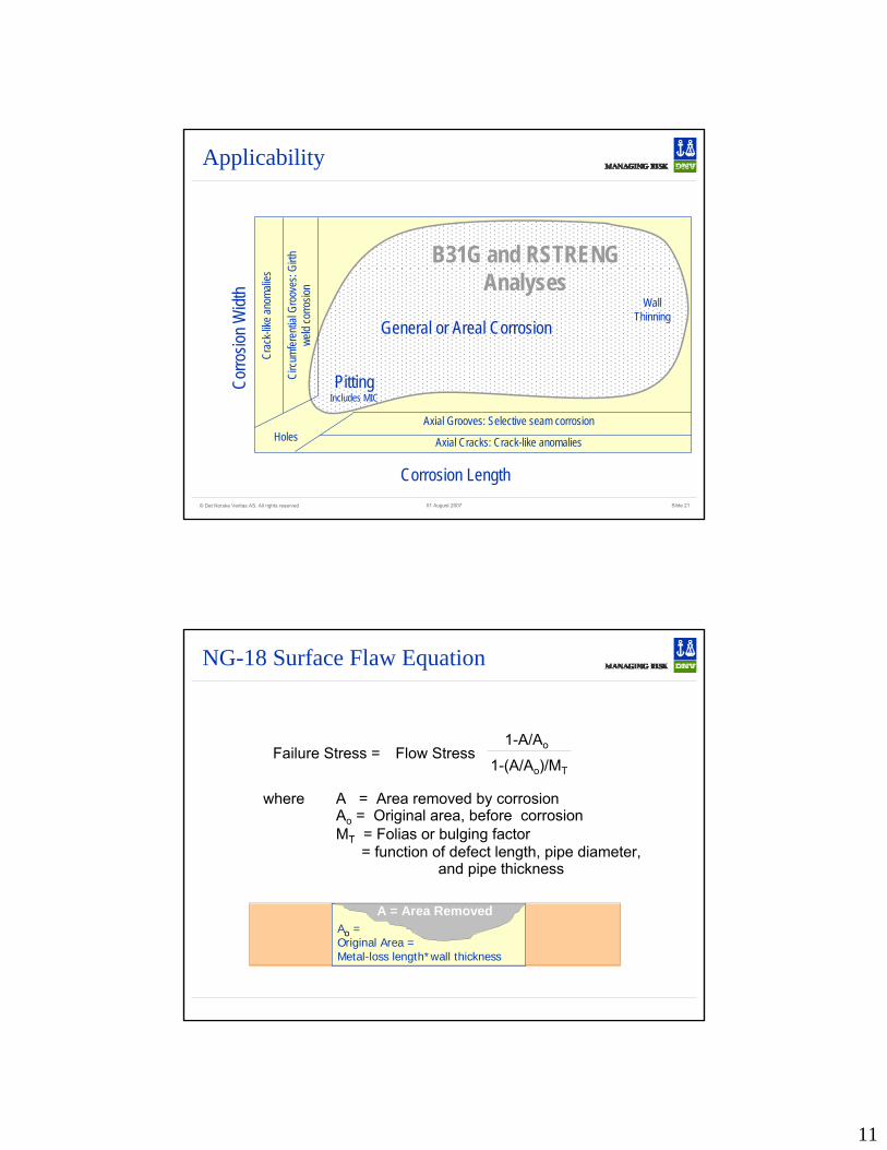
Applicability
Axial Grooves: Selective seam corrosion
Axial Cracks: Crack-like anomalies
Circu
mfer
entia
l Gro
oves
: Girth
we
ld co
rrosio
n
Crac
k-like
anom
alies
Holes
Corrosion Length
Corro
sion W
idth
PittingIncludes MIC
Wall Thinning
General or Areal Corrosion
B31G and RSTRENG Analyses
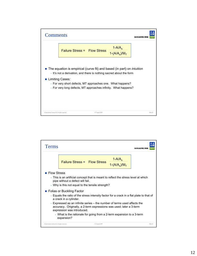
Ao = Original Area = Metal-loss length*wall thickness
NG-18 Surface Flaw Equation
A = Area Removed
1-A/Ao
1-(A/Ao)/MTFlow StressFailure Stress =
A = Area removed by corrosionAo = Original area, before corrosionMT = Folias or bulging factor
where
= function of defect length, pipe diameter,and pipe thickness
12
© Det Norske Veritas AS. All rights reserved Slide 2301 August 2007
Comments
The equation is empirical (curve fit) and based (in part) on intuition- It’s not a derivation, and there is nothing sacred about the form
Limiting Cases:- For very short defects, MT approaches one. What happens?- For very long defects, MT approaches infinity. What happens?
1-A/Ao
1-(A/Ao)/MTFlow StressFailure Stress =
© Det Norske Veritas AS. All rights reserved Slide 2401 August 2007
Terms
Flow Stress- This is an artificial concept that is meant to reflect the stress level at which
pipe without a defect will fail.- Why is this not equal to the tensile strength?
Folias or Buckling Factor- Equals the ratio of the stress intensity factor for a crack in a flat plate to that of
a crack in a cylinder.- Expressed as an infinite series – the number of terms used affects the
accuracy. Originally, a 2-term expressions was used; later a 3-term expression was introduced.
- What is the rationale for going from a 2-term expansion to a 3-term expansion?
1-A/Ao
1-(A/Ao)/MTFlow StressFailure Stress =
13
A = Area Removed
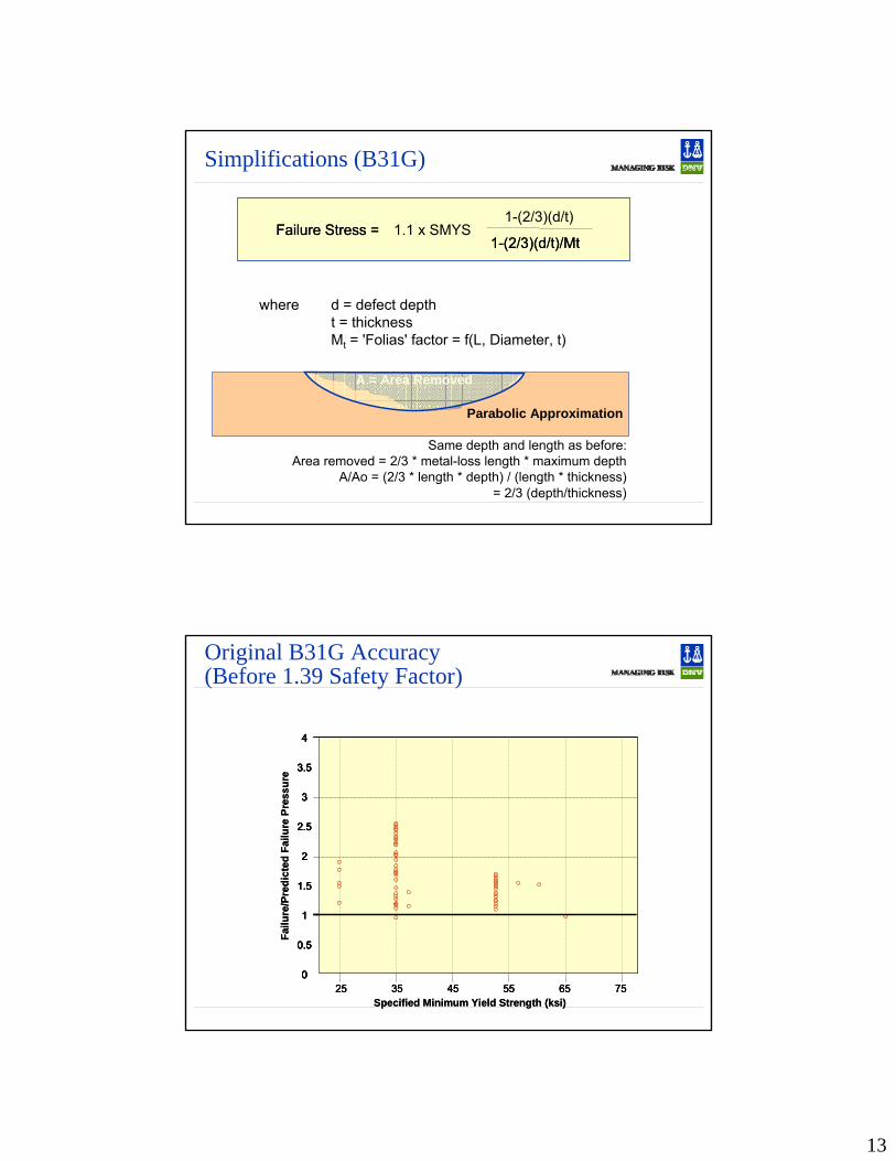
Simplifications (B31G)
d = defect deptht = thicknessMt = 'Folias' factor = f(L, Diameter, t)
where
1-(2/3)(d/t)
1-(2/3)(d/t)/MtFailure Stress =
1-(2/3)(d/t)/Mt1.1 x SMYSFailure Stress =
Parabolic Approximation
Same depth and length as before:Area removed = 2/3 * metal-loss length * maximum depth
A/Ao = (2/3 * length * depth) / (length * thickness)= 2/3 (depth/thickness)
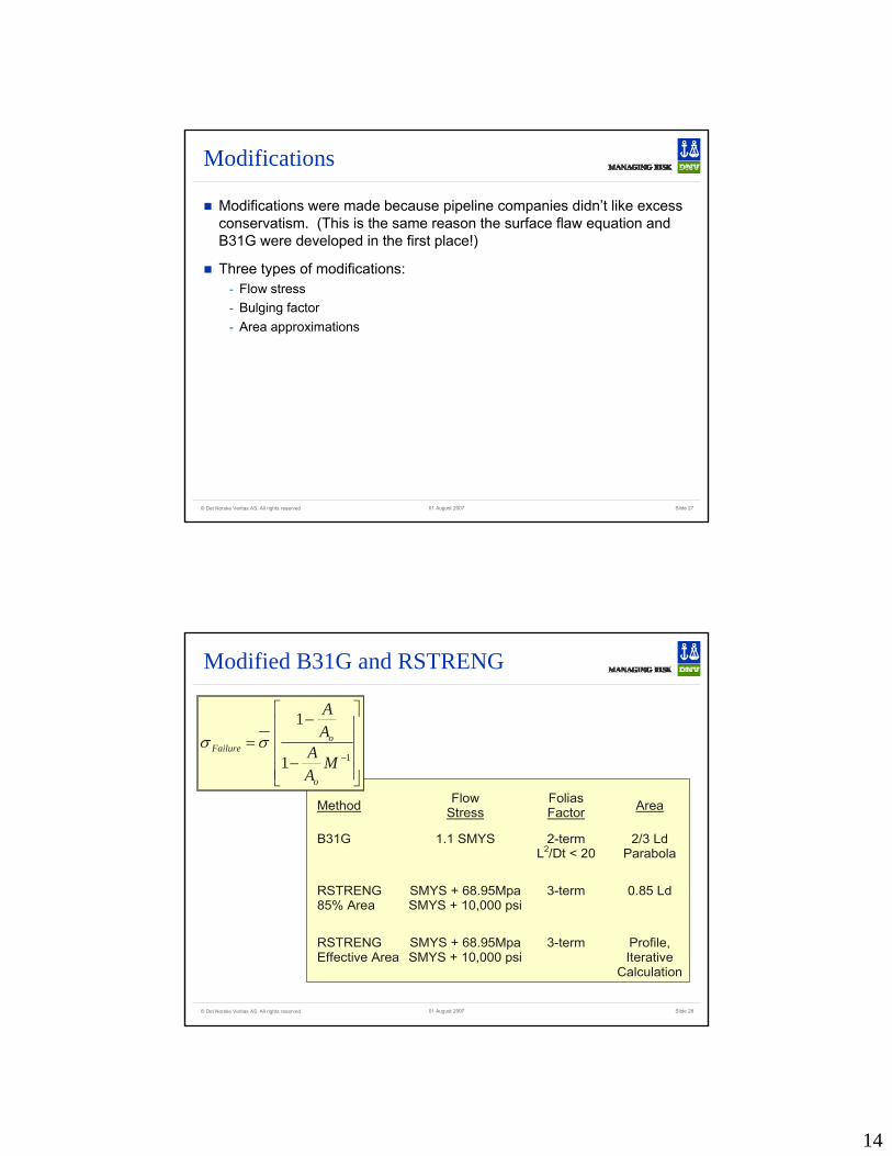
Original B31G Accuracy(Before 1.39 Safety Factor)
25 35 45 55 65 75
2.5
2
1.5
0.5
1
0
3
3.5
4
Specified Minimum Yield Strength (ksi)
Failu
re/P
redi
cted
Fai
lure
Pre
ssur
e
25 35 45 55 65 7525 35 45 55 65 75
2.5
2
1.5
0.5
1
0
3
3.5
4
2.5
2
1.5
0.5
1
0
3
3.5
4
2.5
2
1.5
0.5
1
0
3
3.5
4
Specified Minimum Yield Strength (ksi)
Failu
re/P
redi
cted
Fai
lure
Pre
ssur
e
14
© Det Norske Veritas AS. All rights reserved Slide 2701 August 2007
Modifications
Modifications were made because pipeline companies didn’t like excess conservatism. (This is the same reason the surface flaw equation and B31G were developed in the first place!)
Three types of modifications:- Flow stress- Bulging factor- Area approximations
© Det Norske Veritas AS. All rights reserved Slide 2801 August 2007
Modified B31G and RSTRENG
Method Flow Stress
Folias Factor Area
B31G 1.1 SMYS 2-term L2/Dt < 20
2/3 Ld Parabola
RSTRENG 85% Area
SMYS + 68.95MpaSMYS + 10,000 psi
3-term
0.85 Ld
RSTRENG Effective Area
SMYS + 68.95MpaSMYS + 10,000 psi
3-term
Profile, Iterative
Calculation
⎥⎥⎥⎥
⎦
⎤
⎢⎢⎢⎢
⎣
⎡
−
−=
−11
1
MAA
AA
o
oFailure σσ
15
© Det Norske Veritas AS. All rights reserved Slide 2901 August 2007
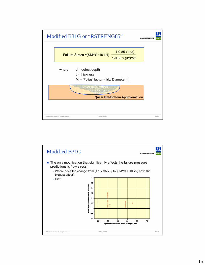
Modified B31G or “RSTRENG85”
A = Area Removed
t = thicknessMt = 'Folias' factor = f(L, Diameter, t)
d = defect depthwhere
1-0.85 x (d/t)Failure Stress =
1-0.85 x (d/t)/Mt(SMYS+10 ksi)Failure Stress =
Quasi Flat-Bottom Approximation
© Det Norske Veritas AS. All rights reserved Slide 3001 August 2007
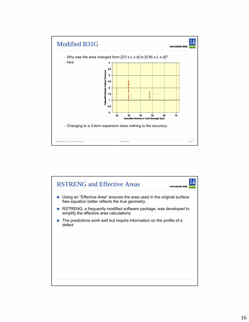
Modified B31G
The only modification that significantly affects the failure pressure predictions is flow stress:
- Where does the change from [1.1 x SMYS] to [SMYS + 10 ksi] have the biggest effect?
- Hint:
25 35 45 55 65 75
2.5
2
1.5
0.5
1
0
3
3.5
4
Specified Minimum Yield Strength (ksi)
Failu
re/P
redi
cted
Fai
lure
Pre
ssur
e
25 35 45 55 65 7525 35 45 55 65 75
2.5
2
1.5
0.5
1
0
3
3.5
4
2.5
2
1.5
0.5
1
0
3
3.5
4
2.5
2
1.5
0.5
1
0
3
3.5
4
Specified Minimum Yield Strength (ksi)
Failu
re/P
redi
cted
Fai
lure
Pre
ssur
e
16
© Det Norske Veritas AS. All rights reserved Slide 3101 August 2007
Modified B31G
- Why was the area changed from [2/3 x L x d] to [0.85 x L x d]? - Hint:
- Changing to a 3-term expansion does nothing to the accuracy.
25 35 45 55 65 75
2.5
2
1.5
0.5
1
0
3
3.5
4
Specified Minimum Yield Strength (ksi)
Failu
re/P
redi
cted
Fai
lure
Pre
ssur
e
25 35 45 55 65 7525 35 45 55 65 75
2.5
2
1.5
0.5
1
0
3
3.5
4
2.5
2
1.5
0.5
1
0
3
3.5
4
2.5
2
1.5
0.5
1
0
3
3.5
4
Specified Minimum Yield Strength (ksi)
Failu
re/P
redi
cted
Fai
lure
Pre
ssur
e
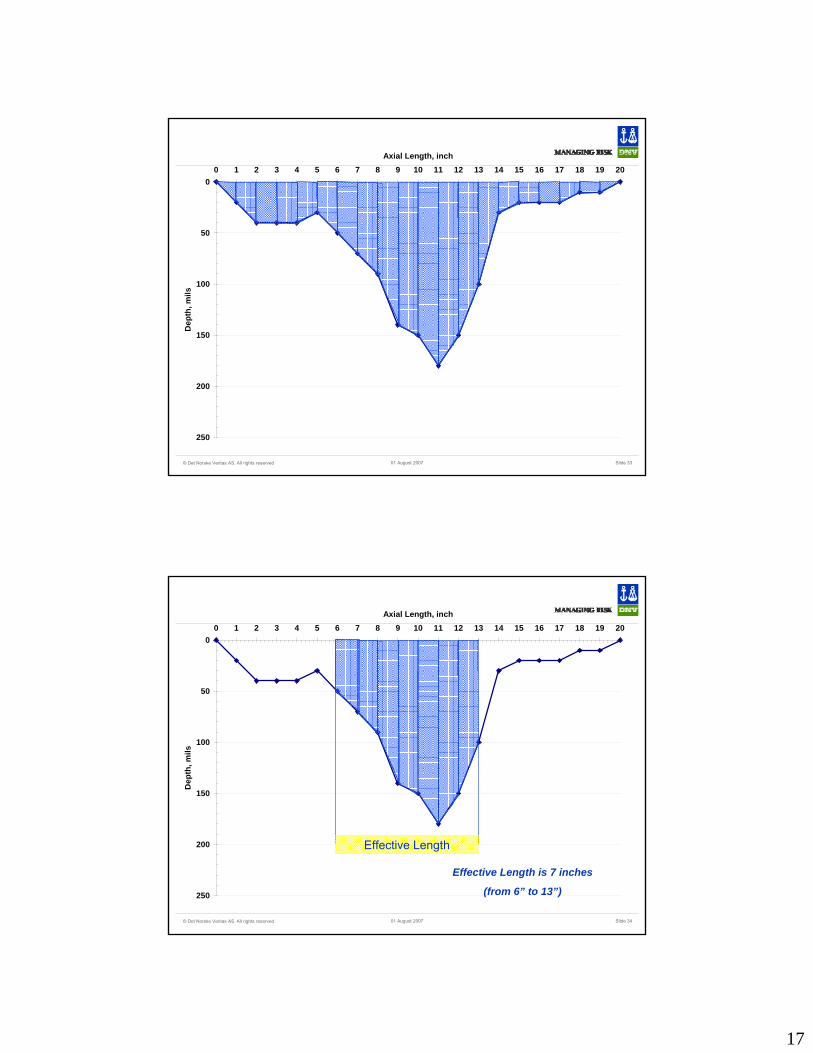
RSTRENG and Effective Areas
Using an “Effective Area” ensures the area used in the original surface-flaw equation better reflects the true geometry.
RSTRENG, a frequently modified software package, was developed to simplify the effective area calculations
The predictions work well but require information on the profile of a defect
17
© Det Norske Veritas AS. All rights reserved Slide 3301 August 2007
0
50
100
150
200
250
0 1 2 3 4 5 6 7 8 9 10 11 12 13 14 15 16 17 18 19 20Axial Length, inch
Dep
th, m
ils
© Det Norske Veritas AS. All rights reserved Slide 3401 August 2007
0
50
100
150
200
250
0 1 2 3 4 5 6 7 8 9 10 11 12 13 14 15 16 17 18 19 20Axial Length, inch
Dep
th, m
ils
Effective Length
Effective Length is 7 inches
(from 6” to 13”)
18
© Det Norske Veritas AS. All rights reserved Slide 3501 August 2007
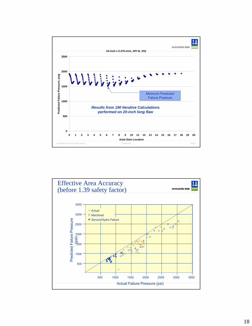
24-inch x 0.375-inch, API 5L X52
0
500
1000
1500
2000
2500
0 1 2 3 4 5 6 7 8 9 10 11 12 13 14 15 16 17 18 19 20Axial Start Location
Pred
icte
d Fa
ilure
Pre
ssur
e, p
sig
Results from 190 Iterative Calculations performed on 20-inch long flaw
Minimum PredictedFailure Pressure
Effective Area Accuracy(before 1.39 safety factor)
1000500 1500 2000 2500 35003000
Actual Failure Pressure (psi)
1000
500
1500
2000
2500
3500
3000
Pre
dict
ed F
ailu
re P
ress
ure
(psi
)
Actual CorrosionMachined DefectService/Hydro Failure
19
Comments on B31G And RSTRENG
Each assumes failure by ductile deformation and cannot be used in low toughness regions (e.g., welds) or for cracks or crack-like
Each assumes failure due to pressure overload and cannot be usedwhere axial loads are high
They are also not appropriate for defects with large circumferential extents
They are sometimes unconservative for short deep defects that fail by leaking (and B31G cannot be used for defects greater than 60 to 80 percent deep)
They do not consider multiple or spiral defects
Analysis Methods for CracksPart 1
(and low toughness materials)
20
© Det Norske Veritas AS. All rights reserved Slide 3901 August 2007
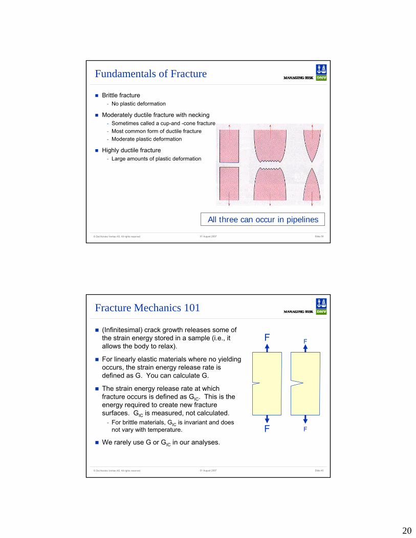
Fundamentals of Fracture
Brittle fracture- No plastic deformation
Moderately ductile fracture with necking- Sometimes called a cup-and -cone fracture- Most common form of ductile fracture- Moderate plastic deformation
Highly ductile fracture- Large amounts of plastic deformation
All three can occur in pipelines
© Det Norske Veritas AS. All rights reserved Slide 4001 August 2007
Fracture Mechanics 101
(Infinitesimal) crack growth releases some of the strain energy stored in a sample (i.e., it allows the body to relax).
For linearly elastic materials where no yielding occurs, the strain energy release rate is defined as G. You can calculate G.
The strain energy release rate at which fracture occurs is defined as GIC. This is the energy required to create new fracture surfaces. GIC is measured, not calculated.
- For brittle materials, GIC is invariant and does not vary with temperature.
We rarely use G or GIC in our analyses.
F
F
F
F
21
© Det Norske Veritas AS. All rights reserved Slide 4101 August 2007
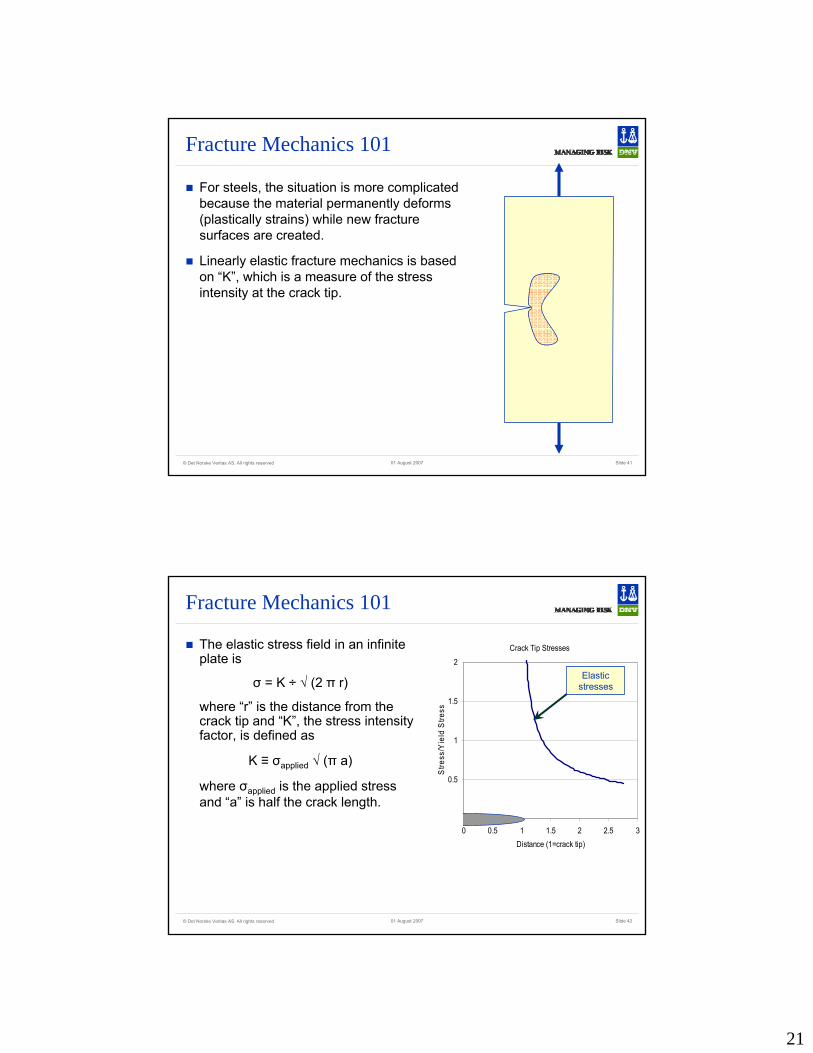
Fracture Mechanics 101
For steels, the situation is more complicated because the material permanently deforms (plastically strains) while new fracture surfaces are created.
Linearly elastic fracture mechanics is based on “K”, which is a measure of the stress intensity at the crack tip.
© Det Norske Veritas AS. All rights reserved Slide 4201 August 2007
Crack Tip Stresses
0
0.5
1
1.5
2
0 0.5 1 1.5 2 2.5 3Distance (1=crack tip)
Stre
ss/Y
ield
Stre
ss
Elastic stresses
Fracture Mechanics 101
The elastic stress field in an infinite plate is
σ = K ÷ √ (2 π r)
where “r” is the distance from the crack tip and “K”, the stress intensity factor, is defined as
K ≡ σapplied √ (π a)
where σapplied is the applied stress and “a” is half the crack length.
22
© Det Norske Veritas AS. All rights reserved Slide 4301 August 2007
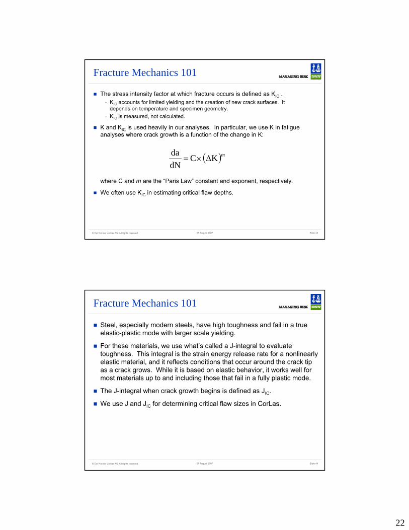
Fracture Mechanics 101
The stress intensity factor at which fracture occurs is defined as KIC . - KIC accounts for limited yielding and the creation of new crack surfaces. It
depends on temperature and specimen geometry. - KIC is measured, not calculated.
K and KIC is used heavily in our analyses. In particular, we use K in fatigue analyses where crack growth is a function of the change in K:
where C and m are the “Paris Law” constant and exponent, respectively.
We often use KIC in estimating critical flaw depths.
( )mK C dNda
Δ×=
© Det Norske Veritas AS. All rights reserved Slide 4401 August 2007
Fracture Mechanics 101
Steel, especially modern steels, have high toughness and fail in a true elastic-plastic mode with larger scale yielding.
For these materials, we use what’s called a J-integral to evaluate toughness. This integral is the strain energy release rate for a nonlinearly elastic material, and it reflects conditions that occur around the crack tip as a crack grows. While it is based on elastic behavior, it works well for most materials up to and including those that fail in a fully plastic mode.
The J-integral when crack growth begins is defined as JIC.
We use J and JIC for determining critical flaw sizes in CorLas.
23
© Det Norske Veritas AS. All rights reserved Slide 4501 August 2007
Summary Point
Fracture mechanics generally deals with materials that fail before reaching fully plastic (limit load) conditions. It is based on the energy used up in the vicinity of a crack tip as the crack grows.
We primarily use K, KIC, J, and JIC in our analyses. - K and KIC are for fatigue analyses for materials that have limited yielding
before failure.- J and JIC are used for determining critical flaw sizes. We sometimes use KIC
to estimate critical flaw sizes when there is limited yielding.
© Det Norske Veritas AS. All rights reserved Slide 4601 August 2007
Stopping Point
The next lecture will cover how analysis methods take into account different forms of K, J, KIC and JIC for pipeline materials.


![Automatic Audio Defect Detection · 3 Defect types and detection methods 11 1 1.5 2 2.5 3 3.5-0.4-0.2 0 0.2 0.4 position in file [sec] waveform detected defect Figure 3.2:Example](https://img.pdfslide.us/doc/110x75/603d87a91bb7437a722f9596/automatic-audio-defect-3-defect-types-and-detection-methods-11-1-15-2-25-3-35-04-02.jpg)


![Defect Characterisation from Limited View Pipeline Radiography · Figure 1: Double Wall methods of radiographic imaging of pipelines for corrosion (EN 16407: part 2 [3]); ... isation](https://img.pdfslide.us/doc/110x75/5af7dc077f8b9a9e5991460d/defect-characterisation-from-limited-view-pipeline-radiography-1-double-wall-methods.jpg)