Embed Size (px)
Citation preview
Development of costing tool for
Outokumpu Stainless Oy
Timo Saarela
Tuotantotalouden koulutusohjelman opinnäytetyö
Insinööri (AMK)
TORNIO 2015

2
FOREWORDS
First of all I would like to say the biggest thanks to my family, especially to my wife
Jaana, who gave me opportunity to start, continue and complete these studies. Secondly,
I have been lucky to have, in a row two managers in Outokumpu, who have given their
full support for my studies, so thanks to Juha Orasvuo and Steve Hudson. I would also
say greatest thanks to my thesis supervisor Timo Huhtala giving great guidance and
support to succeed in this work.
Thirdly, I would say my thanks to Outokumpu Oyj Human Resources to be able to use
time away from my work for these studies and to use internal resources to study and
support this work. Another good example of Outokumpu supporting personal studies is
the Tornio Works library, where I was able to lend almost every book necessary for my
studies.
Last but not least I would say thanks to the great school of Lapland University of Ap-
plied Sciences. In this great university I had the opportunity to do my studies remotely
and I was able to combine my studies with my work, hobbies and family.
Tornio on 9th
of February, 2015
Timo Saarela

3
TIIVISTELMÄ
KEMI-TORNION AMMATTIKORKEAKOULU, Koulutusala
Koulutusohjelma: Tuotantotalous
Opinnäytetyön tekijä(t): Timo Saarela
Opinnäytetyön nimi: Hinnoittelutyökalun kehitys Outokumpu Stainless Oy’lle
Sivuja (joista liitesivuja): 48 (0)
Päiväys: 9.2.2015
Opinnäytetyön ohjaaja(t):
Juha Kaarela Lapin AMK,
Timo Huhtala Outokumpu Oyj
Toimeksiantonani oli kehittää uusi hinnoittelutyökalu Outokumpu Stainless Oy’n
myynnin käyttöön. Hinnoittelutyökaluun liittyvät luottamukselliset tekstit ja asiakir-
jat on jätetty pois julkisesta opinnäytetyöstä.
Opinnäytetyöni sisältää hinnoittelun ja kannattavuuden teoriaosuuden. Hinnoittelua
ja kannattavuutta on tarkasteltu myynnin, tuotannon ja raaka-ainehankinnan näkö-
kulmista. Teoriaosuudessa käsitellään mm. hintastrategiaa, hintapolitiikkaa, kontri-
buutiota, liikevoittoa ja hinnoittelun toimintaa käytännössä. Opinnäytetyöni sisältää
myös teoriaosuuden regressioanalyysistä ja Outokumpu Oyj’n kannattavuuslasken-
nasta.
Teoriaosuus hinnoittelusta ja kannattavuudesta toimii hyvänä taustamateriaalina kai-
kille yrityksen hinnoittelusta ja kannattavuudesta kiinnostuneille henkilöille. Opin-
näytetyöni teoriaosuudessa keskitytään hinnoittelun ja kannattavuuden perusasioihin.
Hinnoittelun ja kannattavuuden teoriaa selvitin lukemalla hinnoitteluun liittyviä kir-
joja, hyödyntämällä internetiä ja Outokummun intranetiä.
Toimeksiannon lopputuloksena syntyi uusi myynnin hinnoittelutyökalu ja se on nyt
Outokumpu Stainless Oy’n käytössä.
Asiasanat: Opinnäytetyön sisällön perusteella valitaan 3 - 7 asiasanaa YSA:n eli ylei-
sen suomalaisen asiasanaston mukaan. Sanat erotetaan toisistaan pilkulla.
4
ABSTRACT
KEMI-TORNIO UNIVERSITY OF APPLIED SCIENCES, Education
Degree programme:
Bachelor of Engineering , Industrial Engineering and Management
Author(s): Timo Saarela
Thesis title: Development of Costing Tool for Outokumpu Stainless Oy
Pages (of which appendixes): 48 (0)
Date: 9th
of February 2015
Thesis instructor(s):
Juha Kaarela Lapland University of Applied Sciences,
Timo Huhtala Outokumpu Oyj
This assignment was to review and develop existing costing tool for Outokumpu
Stainless Oy. Confidential material of costing tool has been left out of the public the-
sis.
This thesis contains theory and empirical part of pricing and profitability, where theo-
ry is review on sales, production and raw-material purchasing point of view. Pricing
and profitability theory contains; pricing strategy, pricing policy, contribution, operat-
ing profit and practical pricing. This thesis introduces basics of regression and Ou-
tokumpu Vertical Profitability System.
The theory section of thesis offers background material for all who are interested in
company pricing. Details in Pricing, regression and vertical profitability theory stays
on basic level. Main sources of the theory part were books and articles of them and
finding information from Internet and company intranet.
As the result of the assignment, new developed costing tool was launched for Ou-
tokumpu Stainless Oy.
Asiasanat: Opinnäytetyön sisällön perusteella valitaan 3 - 7 asiasanaa YSA:n eli ylei-
sen suomalaisen asiasanaston mukaan. Sanat erotetaan toisistaan pilkulla.
5
TABLE OF CONTENTS
TIIVISTELMÄ ................................................................................................................. 3
ABSTRACT ...................................................................................................................... 4
TABLE OF CONTENTS .................................................................................................. 5
USED SYMBOLS AND ABBREVIATIONS ................................................................. 7
1 INTRODUCTION ........................................................................................................ 8
2 PRICING THEORY ................................................................................................... 10
2.1 Background ........................................................................................................... 10
2.2 Pricing three levels ................................................................................................ 12
2.3 Variable and fixed costs ........................................................................................ 13
3 REGRESSION ............................................................................................................ 15
3.1 Simple regression model ....................................................................................... 15
3.2 Multiple regression model .................................................................................... 15
3.3 Correlation ............................................................................................................ 16
4 COSTING TOOL STATUS AND DEVELOPMENT ............................................... 17
4.1 Requirement for new tool ..................................................................................... 17
4.2 Business benefits ................................................................................................... 18
4.3 Linkages ................................................................................................................ 19
4.3.1 Vertical profitability system ....................................................................................... 19
4.3.2 Metal market prices and currencies ........................................................................... 22
4.3.3 Freights ...................................................................................................................... 23
4.3.4 Forecasted raw material prices ................................................................................... 23
4.4 Development limitations ....................................................................................... 23
4.5 Schedule ................................................................................................................ 24
4.6 Budget and resources ............................................................................................ 24
6
5 DEVELOPMENT DELIVERABLES ........................................................................ 25
5.1 Interface................................................................................................................. 27
5.1.1 End user selections ..................................................................................................... 27
5.1.2 Results ........................................................................................................................ 28
5.2 Raw material costing model .................................................................................. 30
5.3 Regression model for fixed cost ............................................................................ 33
5.4 Regression models into calculation master ........................................................... 34
5.5 Sensitives of conversion costs ............................................................................... 34
5.5.1 Thickness ................................................................................................................... 34
5.5.2 Grade .......................................................................................................................... 35
5.5.3 Finish.......................................................................................................................... 36
5.5.4 Width.......................................................................................................................... 36
5.5.5 Shape .......................................................................................................................... 37
5.5.6 Edge ........................................................................................................................... 38
5.5.7 Nickel and Chrome .................................................................................................... 39
5.6 Evaluation of conversion cost results .................................................................... 39
5.7 Freight model ........................................................................................................ 41
6 UPDATE PROCESS .................................................................................................. 42
6.1 Raw material and currency exchange rate update process .................................... 42
6.2 Raw material cost model update ........................................................................... 42
6.3 Conversion cost model update .............................................................................. 43
6.4 Freight cost model update ..................................................................................... 43
7 OTHER ACTIVITIES ................................................................................................ 45
8 SUMMARY ................................................................................................................ 46
9 CONTEMPLATION................................................................................................... 47
LIST OF REFERENCES ................................................................................................ 48
7
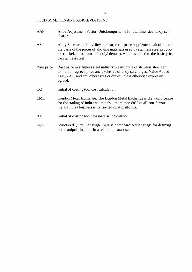
USED SYMBOLS AND ABBREVIATIONS
AAF Alloy Adjustment Factor, Outokumpu name for Stainless steel alloy sur-
charge.
AS Alloy Surcharge. The Alloy surcharge is a price supplement calculated on
the basis of the prices of alloying materials used by stainless steel produc-
ers (nickel, chromium and molybdenum), which is added to the basic price
for stainless steel.
Base price Base price in stainless steel industry means price of stainless steel per
tonne. It is agreed price and exclusive of alloy surcharges, Value Added
Tax (VAT) and any other taxes or duties unless otherwise expressly
agreed.
CC Initial of costing tool cost calculation.
LME London Metal Exchange. The London Metal Exchange is the world centre
for the trading of industrial metals – more than 80% of all non-ferrous
metal futures business is transacted on it platforms.
RM Initial of costing tool raw material calculation.
SQL Structured Query Language. SQL is a standardized language for defining
and manipulating data in a relational database.
8
1 INTRODUCTION
Stainless Steel manufacturing business, together with almost all the industrial business
especially in Europe is having challenging times. Stainless steel industry has met partic-
ular increase of competition during last five – six years. Together with economic crisis
in Europe, Stainless steel industry gets new challengers from Asia, to compete with
their customer. Increase of Asian imports on market has roiled the stainless steel mar-
kets in Europe. Especially Asian Stainless steel manufacturers are dumping the stainless
steel material into Europe on very low prices.
Stainless steel has been strongly growing business in recent decades and, according to
independent market researchers, growth will continue in future. In the past, stainless
business was production constraint (i.e. demand was constantly exceeding the global
stainless steel production capacity), thus natural focus in strategy was to get most out of
mills and get production volumes high. Following recent, very strong Chinese players
entry to the stainless markets after year 2000, in 2005 global production output of stain-
less steel was first time reported to exceed the global demand.
Nowadays the overcapacity is unsustainable for all players and Outokumpu is facing
tough competition in all regions. Stainless steel producers are thus in tight price compe-
tition and racing to be more and more cost competitive in order to survive. In this mar-
ket situation, in addition to get as much as possible volume sold, it is utmost important
simultaneously to manage the prices at reasonable levels. In order to have clear view on
bottom prices, it is vital to have updated view on current variable and fixed cost. That
sets a requirement of very regularly updated review of raw-materials, freights and other
cost elements per produced stainless steel grade.
Based on this challenging time in Stainless steel industry, Outokumpu Stainless Oy re-
quires costing tool, which contains accurate information of company variable and fixed
costs. This tool needs to deliver the best possible results for sales man to use, in order to
win customers inquiry, by offering mutual satisfactory trading. In this thesis, this tool
for Outokumpu Stainless Oy is introduced.

9
In addition to the costing tool this thesis contains pricing theory in chapter two, regres-
sion theory in chapter three. In chapter four there is introduction of Outokumpu corpo-
rate wide vertical profitability system. Vertical profitability system is introduced in this
thesis since costing tool uses its cost data. Then in chapter five costing tool status and
development are to be found. This chapter introduces current status and developed parts
of costing tool. Chapter five contains introduction of business requirements and bene-
fits, overview of this development requirements.
Chapter six explains details of this costing tool development deliverables. Chapter six
introduces also costing tool interface and its changes on this development. Here we can
also see how end user selections will work in new tool and how the end user selections
impact costing tool results. There is also introduction of added production grades and as
well as how raw material and conversion cost models work. New regression model
within fixed costs and the way how the regression models are transferred into costing
tool calculation master are introduced. Last thing in chapter six is introduction of raw
material cost formulas and freight model.
Chapter seven contains introduction of costing tool update process. Update process ex-
plains how costing tool background data like raw material and conversion cost models
are updated. In addition, there is introduction of freight model update and how input
data is evaluated are to be seen. Chapter eight contains other activities like testing and
training of the tool.
10
2 PRICING THEORY
2.1 Background
Immediately after the end of World War II there has been downward pressure on all the
prices going too high. Some of its roots come from trade cyclical factors – such as slow
economic growth in the Western economies and Japan – that have steered in consumer
spending. There are newer sources as well: the huge increased purchasing power of re-
tailers, such a Wal-Mart, which can therefore pressure suppliers; the internet, which
adds to the transparency of markets by making it easier to compare prices; and role of
China and other burgeoning industrial powers whose low labor costs have driven down
prices for manufactured goods. The one-two punch of trade cycles and newer factors
had weared corporate pricing power and forced frustrated managers to look in every
direction for ways to hold the line. (McKinsey & Company 2014)
In such a business environment, managers might think that it’s mad to talk about raising
prices. We are not talking about raising prices across the board, but the most effective
path is to get prices right for one customer or customer group, one sales transaction at a
time, and to capture more of the price that you already charge. In this sense there is
room for price increases or at least price solidity even in our current difficult markets.
Such an approach to pricing, like transaction pricing, one of the three levels of price
management, was first described and introduced about ten years ago. The idea was to
figure out the real price you charged customers after accounting for a host of discounts,
allowances, rebate, and other deductions. Only then you are able to calculate how much
money, if any, you were making and whether you were charging the right price for each
customer and transaction. (McKinsey & Company 2014)
Patented technologies often can be rapidly copied, and attempts to achieve breakthrough
innovations often fail. What’s left as a basis for competition is execution and smart de-
cision making. Sophisticated analytics enable market leading companies to generate a
new and lasting competitive advantage. This is the way how building and implementing
analytical tool would create competitive differentiation. (Davenport & Harris 2007, 47)

11
There are several ways to approach competitive advantage on pricing by using data.
One approach on pricing analytics is to collect unique data and prospects of customers
over time. Collected data and prospects should be unique, so competitor cannot match
or copy. Another way is to organize, standardize and even manipulate the data and as
result data is in unique format. There is also option for companies to establish own algo-
rithm what can give better and more insightful analyses for pricing decisions. Regard-
less of the analytical approach, companies needs to get competitive advantage of their
analyses. Analytics need to be attached judiciously, them needs to be well executed and
continuously reformed. (Davenport & Harris 2007, 48)
Companies who have successful compete on analytical skills, should have one of the
following four capabilities. (Davenport & Harris 2007, 48)
1. Hard to duplicate. It’s easy for companies to copy another company IT
applications or its products and product related attributes. Quite another thing is
to copy another company processes and their culture. (Davenport & Harris 2007,
48)
2. Unique. There is no one correct way to follow to be an analytical competitor.
Company need to define their unique way of using analytics and their path
should follow and support defined strategy and market position. (Davenport &
Harris 2007, 48)
3. Adaptable for many situations. An analytical organization can apply and use
analytical availability in different, innovative ways. (Davenport & Harris 2007,
48)
4. Better than competition. Even the company in different industries has analytical
skills and their consolidated data is wide and accurate, some of companies are
just better to utilize data than others. (Davenport & Harris 2007, 48)
12
2.2 Pricing three levels
Transaction pricing is introduced as one of the three levels of price management. Alt-
hough to clarify, each level of these pricing levels is related to the other pricing levels.
Secondly pricing action as any on level could easily affect the others as well. Businesses
trying to provide a price benefit to make manager pricing a source of differentiate per-
formance. This can be master of all the three of these levels. (McKinsey & Company
2014)
The widest view of pricing comes from industry price level, where managers must un-
derstand how to supply, demand, understand the costs, regulations and other high-level
factors, how they impact on overall prices. Companies which apply this level of pricing
could avoid unnecessary downward pressure of prices and often become as industry
price leaders. (McKinsey & Company 2014)
The main issue on second level of pricing is a product and/or service, which is relative
to the competition or competitor products and/or services. To make this happen, com-
panies must understand how customers understands all offerings on the market and es-
pecially, which part of product as well as service(s) and nonmaterial goods attributes
drive(s) for purchase decisions. Within this knowledge, companies can create their own
price lists, which accurately impacts the competitive strengths (or weaknesses) of their
offerings. (McKinsey & Company 2014)
Pricing third level, transactional level pricing, company needs to decide the exact price
of each individual order or transaction separately. Starting point of this transactional
pricing is the list of price and what discounts, allowances, payment terms, bonuses and
other incentives should and must be applied or deduct. For majority of companies, the
management of transaction pricing is the most detailed, time-consuming, system-
intensive and energy intensive task involved to get the price advantage from market.
(McKinsey & Company 2014)
13
2.3 Variable and fixed costs
Operating costs could be divided into variable or fixed production costs, with respect to
volume. Both of terms refer for common view of total costs. There is a change in pro-
duced volume and this change has impact on amount of a particular costs element, and
then this element of cost is variable cost. Variable costs are directly related to produce
volume and they will increase if production volume increases. Example of variable
costs is production raw materials, used energy in production, manning time on produc-
tion. (Asish K. Bhattacharyya, pages 288 – 299)
A cost which does not change, even though the produced volume changes can be classi-
fied as fixed cost. There are business resources which need to operate whether there is
production or not. There are three main categories which explain fixed costs:
1) Costs are stable on short period of time, typically a year (Excluding depreciation
and other sunk costs)
2) Costs are stable even the production increases or decreases (for example:
supervision)
3) Costs which are not directly related for production, for example design
engineering.
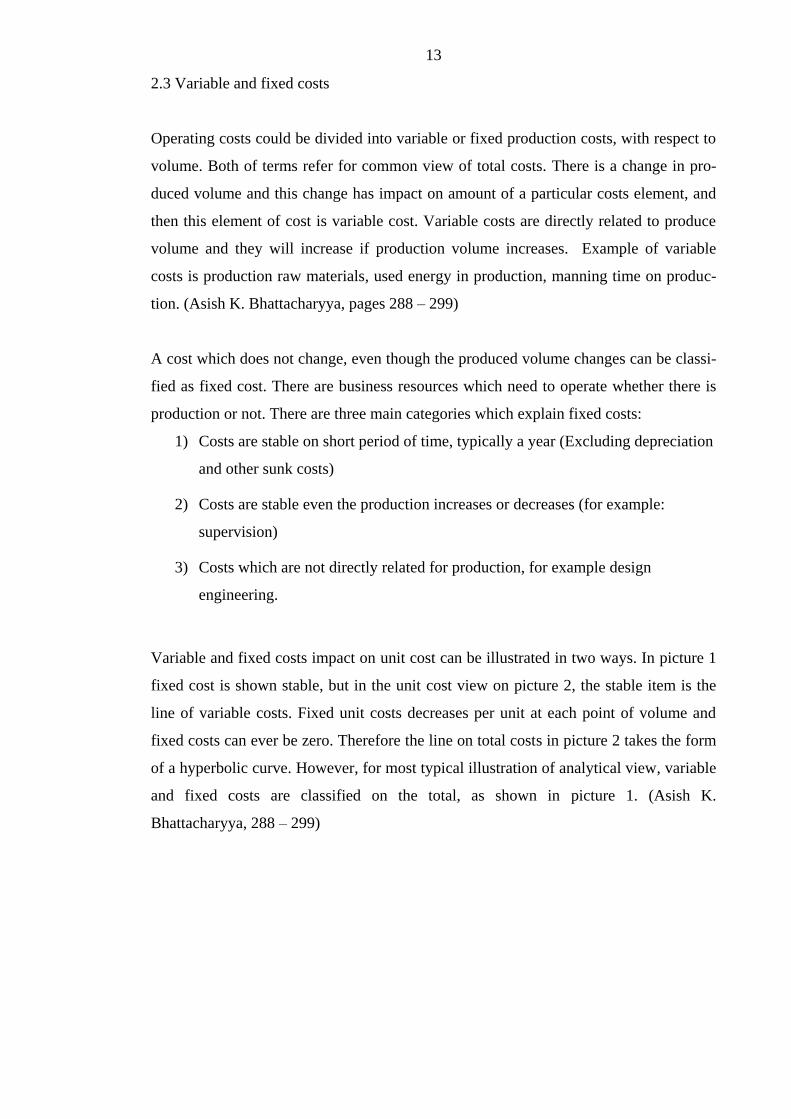
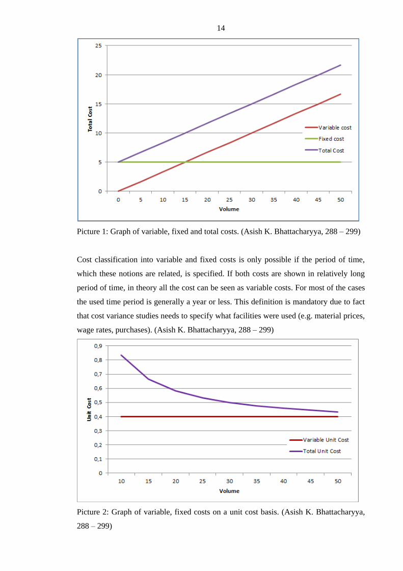
Variable and fixed costs impact on unit cost can be illustrated in two ways. In picture 1
fixed cost is shown stable, but in the unit cost view on picture 2, the stable item is the
line of variable costs. Fixed unit costs decreases per unit at each point of volume and
fixed costs can ever be zero. Therefore the line on total costs in picture 2 takes the form
of a hyperbolic curve. However, for most typical illustration of analytical view, variable
and fixed costs are classified on the total, as shown in picture 1. (Asish K.
Bhattacharyya, 288 – 299)
14
Picture 1: Graph of variable, fixed and total costs. (Asish K. Bhattacharyya, 288 – 299)
Cost classification into variable and fixed costs is only possible if the period of time,
which these notions are related, is specified. If both costs are shown in relatively long
period of time, in theory all the cost can be seen as variable costs. For most of the cases
the used time period is generally a year or less. This definition is mandatory due to fact
that cost variance studies needs to specify what facilities were used (e.g. material prices,
wage rates, purchases). (Asish K. Bhattacharyya, 288 – 299)
Picture 2: Graph of variable, fixed costs on a unit cost basis. (Asish K. Bhattacharyya,
288 – 299)
15
3 REGRESSION
Regression is a statistical event that occurs when repeated measures are made on the
same subject or unit of sample(s). Regression happens due to fact that selected values
are observed with occasional error. Occasional error means a non-methodical variation
in the observed values around a true mean (e.g. occasional measurement error, or occa-
sional flutter in a subject). Systematic error, where the observed values are consistently
unilateral, is not the cause of regression. (Mongomery, Peck & Vining 2012, 12 - 21.)
Regression analysis involves identifying the relationship between a dependent variable
and one or more independent variables. A model of the relationship is hypothesized and
estimates that parameter values are used to develop a regression formula. Amount of
data needs to applied into analyze, before model can be determined as valid model. If
the model is found valid, the regression formula can be used to forecast the value of the
dependent variable given values for the independent variables. (Mongomery, Peck &
Vining 2012, 12 - 21.)
3.1 Simple regression model
In simple linear regression, the model is used to describe the relationship between a
single dependent variable y and a single independent variable x is y = a0 + a1x + k. a0 and
a1 are referred to as the model parameters, and is a probabilistic error term that accounts
for the variability in y that cannot be explained by the linear relationship with x. If the
error term were not present, the model would be deterministic; in that case, knowledge
of the value of x would be sufficient to determine the value of y. (Mongomery, Peck &
Vining 2012, 12 - 21.)
3.2 Multiple regression model
Multiple regression is model, which has two or more explanatory variables on the right
side of the mathematical equation. Multiple regression should be used, if more than one
cause is combined with the effect you wish to perceive. Multiple regression can give
you visibility of more than one factor to make forecast. Comparing multiple regression
for simple regression, it can give you results for only one factor. (Mongomery, Peck &
Vining 2012, 12 - 21.)
16
When we are building regression analyze, it’s crucial do define number of unknown
parameters in the regression model. This process to bring parameters into model is
called fitting the model for data. If you have several independent variables, like in cost-
ing tool, it is classical way to notate variables and the slope parameters like below:
Y = X1 + X2 + … + pXp + error
3.3 Correlation
Correlation and regression analysis are related in the sense that both deal with relation-
ships among variables. The correlation coefficient is a measure of linear association
between two variables. Values of the correlation are always between -1 and +1. A corre-
lation coefficient of +1 indicates that two variables are perfectly related in a positive
linear sense. Correlation coefficient of -1 indicates that two variables are perfectly relat-
ed in a negative linear sense. Correlation coefficient of 0 indicates that there is no linear
relationship between the two variables. Correlation coefficient of |c| < 0,5 is not rele-
vant. Correlation coefficient of 0,6 < |c| < 0,5 would keep remarkable and Correlation
coefficient of |c| > 0,8 is strong correlation (Thomas J. Archdeacon, 1994, 98 - 99.)
For simple linear regression, the sample correlation coefficient is the square root of the
coefficient of determination, with the sign of the correlation coefficient being the same
as the sign of b1, the coefficient of x1 in the estimated regression equation. (Thomas J.
Archdeacon, 1994, 98 - 99.)
Neither regression nor correlation analyses can be interpreted as establishing cause-and-
effect relationships. They can indicate only how or to what extent variables are associat-
ed with each other. The correlation coefficient measures only the degree of linear asso-
ciation between two variables. Any conclusions about a cause-and-effect relationship
must be based on the judgment of the analyst. (Thomas J. Archdeacon, 1994, 98 - 99.)
17
4 COSTING TOOL STATUS AND DEVELOPMENT
In current market situation stainless steel industry suffers from global overcapacity.
This puts pressure on market prices and leads companies to tight cost competition. Thus
there is increasing need for knowing and impacting on company cost structure better
than earlier. To improve cost awareness among sales people, previous version of costing
tool was launched in the beginning of 2010. The aim was to improve the calculation
processes, accuracy and rational behavior of variable and fixed cost levels. Stainless
steel cost structure is heavily driven by direct raw material costs. Especially constantly
changing nickel market price sets requirement for regularly updated information of cost-
ing tool.
Previous version of costing tool was built to fulfill increased requirements of cost in-
formation. Costing tool information was built multidimensional; it is updated regularly
and it gives single point information of Outokumpu Stainless Oy cost. Outokumpu sales
people could use costing tool to examine different profit break-even levels and make
hard decisions on the tightest offers. Tool was mainly used by Outokumpu Stainless Oy
sales. Costing tool was regularly used and highly appreciated among sales people and
thus deserved its status in the sales people’s toolkit.
4.1 Requirement for new tool
Case for change was to develop a new version of Outokumpu Stainless Oy costing tool.
In practical terms, the requirement was further development of calculation procedures of
the tool, planning and documenting updating process, remodeling calculation and inter-
face and finally distribution and end-user training of the tool. In addition to this, gov-
ernance of the tool was documented. Basic calculation principles of the tool were decid-
ed to keep unchanged but e.g. regression model was required to be reviewed and rebuilt
aiming for higher correlation factor of the model. The aim was also to make the update
process as lean and clear as possible.
18
The goal was to create a new version of the tool which offers a possibility to simulate an
impact of key variables on operating profit level. The developed tool was also aiming at
giving a better view of costs between product features and gauges. In the new costing
tool, possibility to simulate metal market price change impacts to the profit / price levels
was required to be kept.
New costing tool with frequent update will support sales people and will make their
work more efficient. Without the information of the tool function, sales people need to
gather similar information from several sources and perform several manual calcula-
tions to make decisions on their offers on daily basis. Manual process is a risk for faults
and when there are many people making calculations, usually calculation principles are
different and results multiple. With this tool, calculation principles are harmonized and
data is readily available. In the development of the costing tool the aim was to re-build
the costing tool, evaluate all the data inputs, implement validation and quality checks.
4.2 Business benefits
Outokumpu was able to recognise three different business benefits from this develop-
ment. Firstly, the new tool gave full transparency to product cost structure. This work
extended profitability levels from contribution down to operating profit. Developed
costing tool reports the most recent costs and pre-calculates different profit level infor-
mation for sales decision makers.
Secondly, the new tool provides better costs accuracy. All the tool calculations were
reviewed and re-modelled, variable cost regression model resulting in higher correla-
tion. Also new regression model for fixed cost was established.
Thirdly, the new tool requires less administration time. Lean and clear update process of
the tool was successfully planned and created. New process model to validate data in-
puts and costing tool results was established and implemented together with help of
raw-material purchase department. Freight costs updating process was established with
logistics department who are accountable for maintaining company freight cost data.
19
Outokumpu costing tool variable (production) and fixed (production, sales & marketing,
depreciation and general administration) costs utilises vertical profitability system cost
information from last six months. Vertical profitability data is queried directly from
Outokumpu data warehouse and contain costs from different production stages. Produc-
tion stages are melting shop, hot rolling, cold rolling mill and finishing lines.
4.3 Linkages
Costing tool has several linkages to existing tools or business processes. These linkages
are vertical profitability, metal market prices and currencies, freight costs and forecast-
ing process of raw material prices.
4.3.1 Vertical profitability system
Since costing tool uses Outokumpu corporate wide profitability tool variable and con-
version cost data, it is introduced in this thesis. In Outokumpu, we have corporate level
“operative” information, i.e. financial data is reworked to better support our planning
and decision making in the areas of sales, profitability and inventory management. Ver-
tical profitability system purpose is simply to better understand the profitability from
the value chain perspective and from the customer viewpoint rather than for internal
businesses and the sales between them. It is intended to support better “operative” deci-
sion making, i.e. on such issues as pricing of stainless steel, capacity allocation, product,
customer and market strategies, route-to-market planning etc. Capacity allocation means
that Outokumpu reserve future production time for certain customer or product se-
quence. Vertical profitability system way of looking profitability is different than e.g
Hyperion Financial management. Vertical profitability system differs from other views
on profit as it could give the very detailed view of Outokumpu product line (invoiced
order split into produced material packages) profitability. (Outokumpu Intranet, 2014)
20
Operative information in Outokumpu means that numbers are aligned to the decisions
our personnel takes in the business (picture 3). For example, when we are looking at a
customer’s profitability, any change in raw material prices or exchange rates from when
the order was taken will then be excluded from the order profit. This time adjusted raw
material calculation method gives fair results for every sales order in system. Being cor-
porate means that numbers cover all units, which are linked into vertical profitability
system and are comparable, or harmonized, so that each reporting unit is treated with
the same principles (this is not the case in Outokumpu’s financial systems which differ
from unit to unit and regionally). (Outokumpu Intranet, 2014)
In the Vertical profitability system Outokumpu can measure the profit created from all
of our sales, in all production stages from melting, hot rolling, cold rolling, finishing,
packing the material and till customer delivery. Vertical profitability system is very im-
portant for Outokumpu as we are steering the company into stable profitability. Instead
of looking at business location by location, vertical profitability system helps by identi-
fying the profit created by our external customers. Vertical profitability looks profitabil-
ity from our external customer perspective and calculates cost route, where material was
melted, where it was rolled, finished and packaged. All previous stages could be pro-
duced in different locations, where vertical profitability system can recognize them and
allocate each steps cost into profitability calculation. Vertical profitability system gives
Outokumpu vies of for example the most profitable segments and customers to sell to. It
also helps identifying the best products and routes to market (from melting mill till cus-
tomer) to serve the customers. (Outokumpu Intranet, 2014)
21
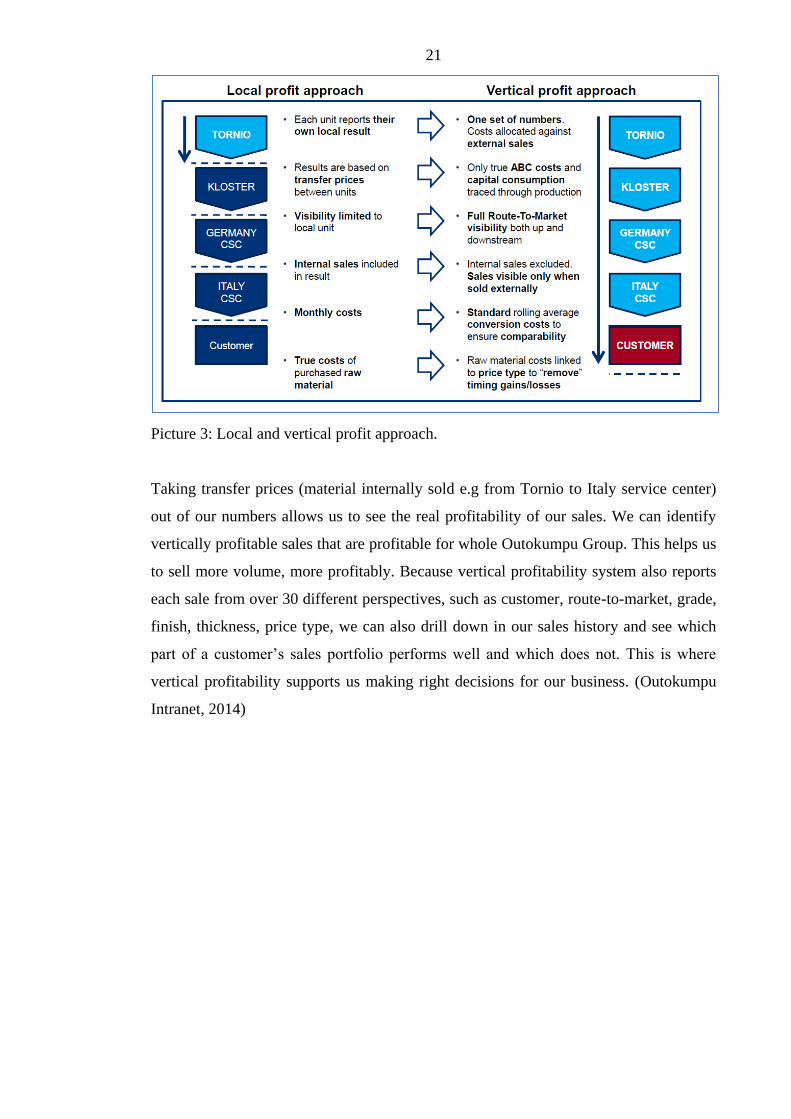
Picture 3: Local and vertical profit approach.
Taking transfer prices (material internally sold e.g from Tornio to Italy service center)
out of our numbers allows us to see the real profitability of our sales. We can identify
vertically profitable sales that are profitable for whole Outokumpu Group. This helps us
to sell more volume, more profitably. Because vertical profitability system also reports
each sale from over 30 different perspectives, such as customer, route-to-market, grade,
finish, thickness, price type, we can also drill down in our sales history and see which
part of a customer’s sales portfolio performs well and which does not. This is where
vertical profitability supports us making right decisions for our business. (Outokumpu
Intranet, 2014)
22
4.3.2 Metal market prices and currencies
Outokumpu raw material costs are determined based on public metal alloy market pric-
es. Depending on purchasing contracts and raw material type (scrap or primary materi-
al) the final prices of raw materials are agreed between Outokumpu and individual sup-
plier. Thus costing tool requires metal market price and more detailed contract infor-
mation as an input. The main alloys are nickel, chromium, molybdenum, iron, copper,
titanium, manganese and niobium. Metal market quotations used for the metals are
listed below. Since metal quotations are US dollar based and costing tool results are in
euros, also USD/EUR exchange rates are required. Costing tool utilizes existing process
of metal market and currency data input into Outokumpu data warehouse metal prices
and currencies (MPC). Metal market and currency data is delivered by Bloomberg.
- Nickel. Nickel is the LME Official Price is the last bid and offer price quoted
during the second Ring session. (London Metal Exchange, 2014)
- Iron $ per Tonne. Iron quotation is published by Metal Bulletin. (Metal Bulletin,
2014)
- Ferro-chrome Lumpy CR charge basis 52% Cr quarterly major European
destinations $ per lb Cr. The settlement of Ferro-chrome is negotiated every
quarter by a large South African ferro-chrome producer and a large European
consumer and has in recent quarters been settled by ferro-chrome producer
Glencore Xstrata and Luxembourg-based stainless steel mill Aperam. (Metal
Bulletin, 2014)
- Molybdenum. Quotation is published by Metal Bulletin. (Metal Bulletin, 2014)
- Copper. Copper is LME Official Settlement Price is the last offer price quoted
during the second Ring session. Quotation is published by Metal Bulletin.
(Metal Bulletin, 2014)
- Titanium. Quotation is published by Metal Bulletin. (Metal Bulleting, 2014)
- Manganese. Quotation is published by Metal Bulletin. (Metal Bulleting, 2014)
- EUR/USD. The reference rate is based on a regular daily concentration
procedure between central banks across Europe and worldwide, which normally
takes place at 2.15 p.m. CET. (European Central Bank, 2014)
23
4.3.3 Freights
Outokumpu Stainless Logistics department is responsible of company stainless material
invoicing and accountable to arrange stainless material deliveries from Tornio mill to
internal or external customer. Logistics department is responsible for negotiation of
freight costs with transport service suppliers and maintaining of the latest freight cost
information. The department updates the latest contracts into local bookkeeping.
Outokumpu Stainless IT collects and consolidates company internal data into local data
warehouse, which includes also freight costs data. This consolidated freight cost data is
then used in costing tool, which shows freight cost per country and per delivery type.
4.3.4 Forecasted raw material prices
Recent metal market prices from the sources described above are used for estimating
profitability of day to day type of short term deals. For long term (above three months in
future) contracts’ profitability estimation, costing tool requires future prices of nickel
alloy. Nickel future values are quoted by London Metal Exchange (LME). Costing tool
utilizes existing process of getting future values of nickel, which has existed due to the
hedging requirement of the metal risk. There was an intention to get all the future prices
of alloys into the costing tool but at the time of writing this thesis, process of getting the
values was not completed.
4.4 Development limitations
Outokumpu is worldwide stainless steel giant company with multiple locations. In the
scope definition phase, extension of the costing tool to cover more units was discussed.
However the decision was made to keep the work focused and re-build costing tool only
for Outokumpu Stainless Oy (located in Tornio).

24
4.5 Schedule
Development of costing tool had following schedule as on table 1:
Table 1: Costing tool development schedule.
4.6 Budget and resources
The work was done by internal resources. Management Information Team which be-
longs to Controllers Corporate Office carried the general meeting costs. Any develop-
ment activity outside these activities, such as travelling costs was carried by home units.
The planned budget was kept.
25
5 DEVELOPMENT DELIVERABLES
Outokumpu Stainless Costing tool development can be split into four main categories.
First category, costing tool development contains: interface, raw material costing model,
conversion costing model and freight model. Second category, costing tool update pro-
cess contains: raw material cost model update, conversion cost model update, and
freight cost model update and validation process planning and implementation. Valida-
tion process planning and implementation deliverable contains; validation of input data,
validation of raw material cost output together with raw material purchase function,
validation of conversion costs and validation of freight costs together with logistics (ta-
ble 2).
Third category, documentation of tool contains; interface documentation, documenta-
tion of RM costs calculation principles, documentation of conversion cost calculation
principles, documentation of tool update process and documentation of data validation
process. Fourth category, user identification and training contains; user identification
and access, end user training material, administration training material and training
schedule and implementation.

26
Table 2: Costing tool development deliverables and their schedule
27
5.1 Interface
5.1.1 End user selections
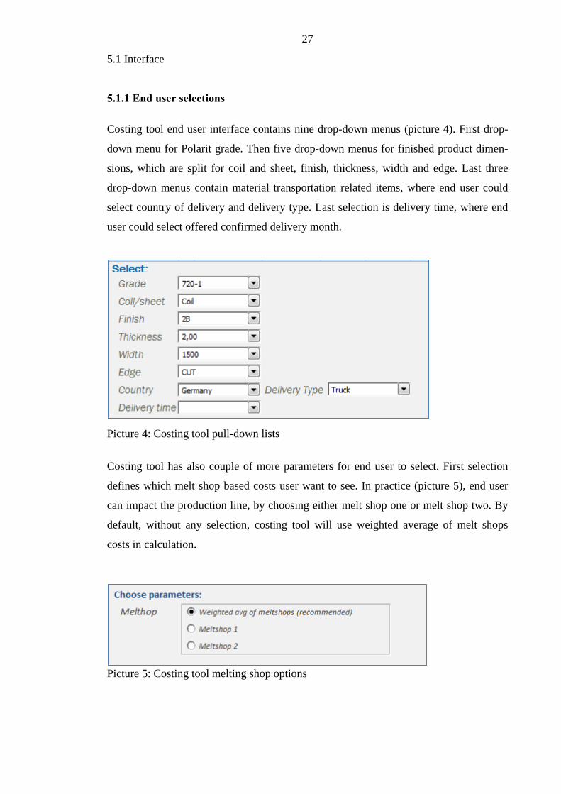
Costing tool end user interface contains nine drop-down menus (picture 4). First drop-
down menu for Polarit grade. Then five drop-down menus for finished product dimen-
sions, which are split for coil and sheet, finish, thickness, width and edge. Last three
drop-down menus contain material transportation related items, where end user could
select country of delivery and delivery type. Last selection is delivery time, where end
user could select offered confirmed delivery month.
Picture 4: Costing tool pull-down lists
Costing tool has also couple of more parameters for end user to select. First selection
defines which melt shop based costs user want to see. In practice (picture 5), end user
can impact the production line, by choosing either melt shop one or melt shop two. By
default, without any selection, costing tool will use weighted average of melt shops
costs in calculation.
Picture 5: Costing tool melting shop options
28
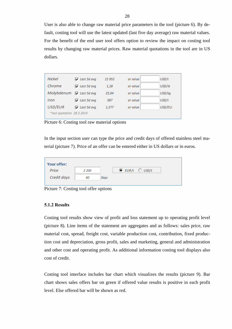
User is also able to change raw material price parameters in the tool (picture 6). By de-
fault, costing tool will use the latest updated (last five day average) raw material values.
For the benefit of the end user tool offers option to review the impact on costing tool
results by changing raw material prices. Raw material quotations in the tool are in US
dollars.
Picture 6: Costing tool raw material options
In the input section user can type the price and credit days of offered stainless steel ma-
terial (picture 7). Price of an offer can be entered either in US dollars or in euros.
Picture 7: Costing tool offer options
5.1.2 Results
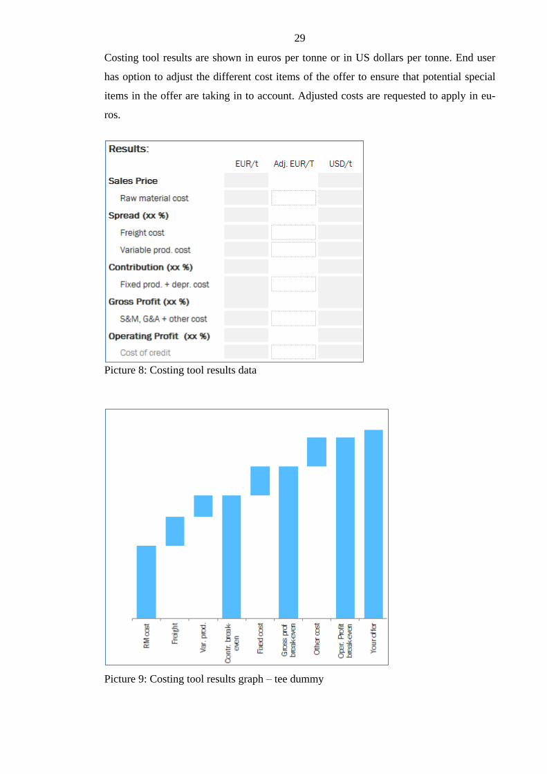
Costing tool results show view of profit and loss statement up to operating profit level
(picture 8). Line items of the statement are aggregates and as follows: sales price, raw
material cost, spread, freight cost, variable production cost, contribution, fixed produc-
tion cost and depreciation, gross profit, sales and marketing, general and administration
and other cost and operating profit. As additional information costing tool displays also
cost of credit.
Costing tool interface includes bar chart which visualizes the results (picture 9). Bar
chart shows sales offers bar on green if offered value results is positive in each profit
level. Else offered bar will be shown as red.
29
Costing tool results are shown in euros per tonne or in US dollars per tonne. End user
has option to adjust the different cost items of the offer to ensure that potential special
items in the offer are taking in to account. Adjusted costs are requested to apply in eu-
ros.
Picture 8: Costing tool results data
Picture 9: Costing tool results graph – tee dummy

30
5.2 Raw material costing model
Raw material cost calculation is mathematical formula, which takes into account alloy
contents of different grades, metal market prices, scrap mixes, contract specific items in
raw material batch pricing and process specific yield. For day to day business (short
term deals) last five days averages of raw materials and currency exchange rates are
used. As stated in the previous chapter for the long term contract profitability evalua-
tions future value of the nickel is used.
Raw material cost calculation inputs are as follows:
Scrap mixes (table 3):
- Polarit grades (Outokumpu Stainless Oy specific stainless steel codes).
- Period displaying year and month when scrap mixes are valid.
- Scrap mix for ferrochrome on melting line one and two
- Scrap mix for nickel on melting line one and two
- Scrap mix for ferromolybdenum on melting line one and two
Table 3: Melting shops line 1 and line 2 scrap mixes
31
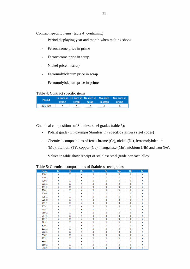
Contract specific items (table 4) containing:
- Period displaying year and month when melting shops
- Ferrochrome price in prime
- Ferrochrome price in scrap
- Nickel price in scrap
- Ferromolybdenum price in scrap
- Ferromolybdenum price in prime
Table 4: Contract specific items
Chemical compositions of Stainless steel grades (table 5):
- Polarit grade (Outokumpu Stainless Oy specific stainless steel codes)
- Chemical compositions of ferrochrome (Cr), nickel (Ni), ferromolybdenum
(Mo), titanium (Ti), copper (Cu), manganese (Mn), niobium (Nb) and iron (Fe).
Values in table show receipt of stainless steel grade per each alloy.
Table 5: Chemical compositions of Stainless steel grades
32
5.3 Conversion cost model
Due to high diversity of stainless steel end products, production costs are affected by
many more than one or two variables. After careful investigation of the raw conversion
cost data combined with the qualitative knowledge of the industry and iteration of the
regression models, six main variables were selected originally to the group of explana-
tory variables. Those variables were: thickness, grade, finish, width, shape and edge.
After further study done in this thesis, contrary to the previous version of costing tool,
yield was decided to drop-out from the variables as it has no or only small impact on
correlation coefficient. Also, the original need of providing possibility to play with yield
of new products (when costing tool was originally launched) was not any more valid.
Conversion cost model consists of two separate multiple regression calculations and one
heavily standardized packaging costs. Multiple regressions are separately built for vari-
able and fixed production costs (the latter including production depreciation).
In this model, thickness is only numerical variable, where others are counted as “dum-
my” variables. When production cost variables were evaluated, finding was that cost of
thickness is exponentially increased, when material is rolled from thick to thinner. Since
used regression model is linear and thickness impact on cost was exponential, there was
need for normalizing thickness values. In this model thickness is normalized by apply-
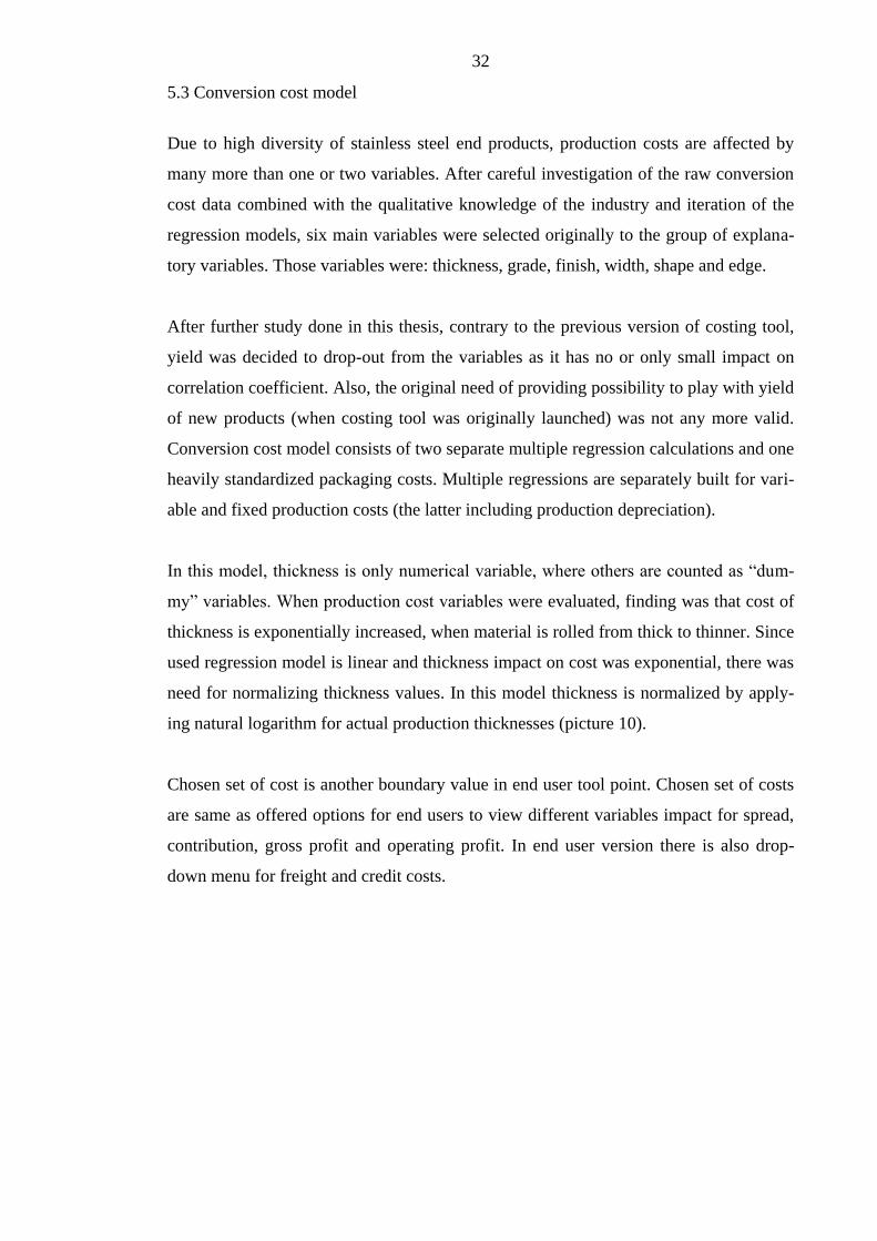
ing natural logarithm for actual production thicknesses (picture 10).
Chosen set of cost is another boundary value in end user tool point. Chosen set of costs
are same as offered options for end users to view different variables impact for spread,
contribution, gross profit and operating profit. In end user version there is also drop-
down menu for freight and credit costs.
33
Picture 10: Natural logarithm of actual thickness
5.3 Regression model for fixed cost
Fixed production cost gives information of production unchanged fixed cost, which will
be stable even there is no production. Fixed production cost contains changes when of-
fered product material gauges changes. Fixed costs contains production, sales & market-
ing, depreciation and all the general administration costs from melting shop, hot rolling
– and cold rolling mill.
By applying production and administration fixed costs, end user can get results of gross-
and operating profit. Added fixed cost will give information for end user, what would
be gained gross- and operating profit, when they are making their offers for customer.
At the offer point it’s crucial to understand how, even the minor change for offer, could
impact our company profitability.
34
5.4 Regression models into calculation master
Costing tool contains business sensitive confidential information. Previous version of
the tool contained different calculation spreadsheets for raw material costs, conversion
costs and freight costs. There was obvious risk that confidential calculation data and
calculation procedures of the costing tool could leak into wrong hands. In the planning
phase of the costing tool deliverables, one of the highest priorities was to improve data
security of the confidential information. The decision was taken to transfer all the pos-
sible calculation procedures outside the user interface. Calculation master file was es-
tablished and only the relevant information was transferred back to end user tool.
5.5 Sensitives of conversion costs
Sensitives for different product gauges are included as additional information for the
costing tool users. The purpose of the sensitivity information is two-folded. On one
hand sensitivity information increases end-users’ awareness of production costs of dif-
ferent products. On the other hand, sensitivity information increases end-users’ aware-
ness of cost item change impact for variable costs. Variable costs sensitives are calcu-
lated for thickness, grade, finish, width, shape and edge. Sensitivity cost information
contain also raw material sensitivity matrix for raw material cost of chosen grade in
relation to nickel and chrome price changes.
5.5.1 Thickness
Thicknesses are divided into twenty different thickness groups. Thickness group on
thick end is rounded into integer of millimeter, where thickness group on thin end has
groups in every 0,1 millimeter. Thickness groups start from 0,50 mm and end on 13,00
mm. On costing tool regression model these thickness groups are not used, but regres-
sion model includes in all the actual thicknesses (adjusted by natural logarithm).
35
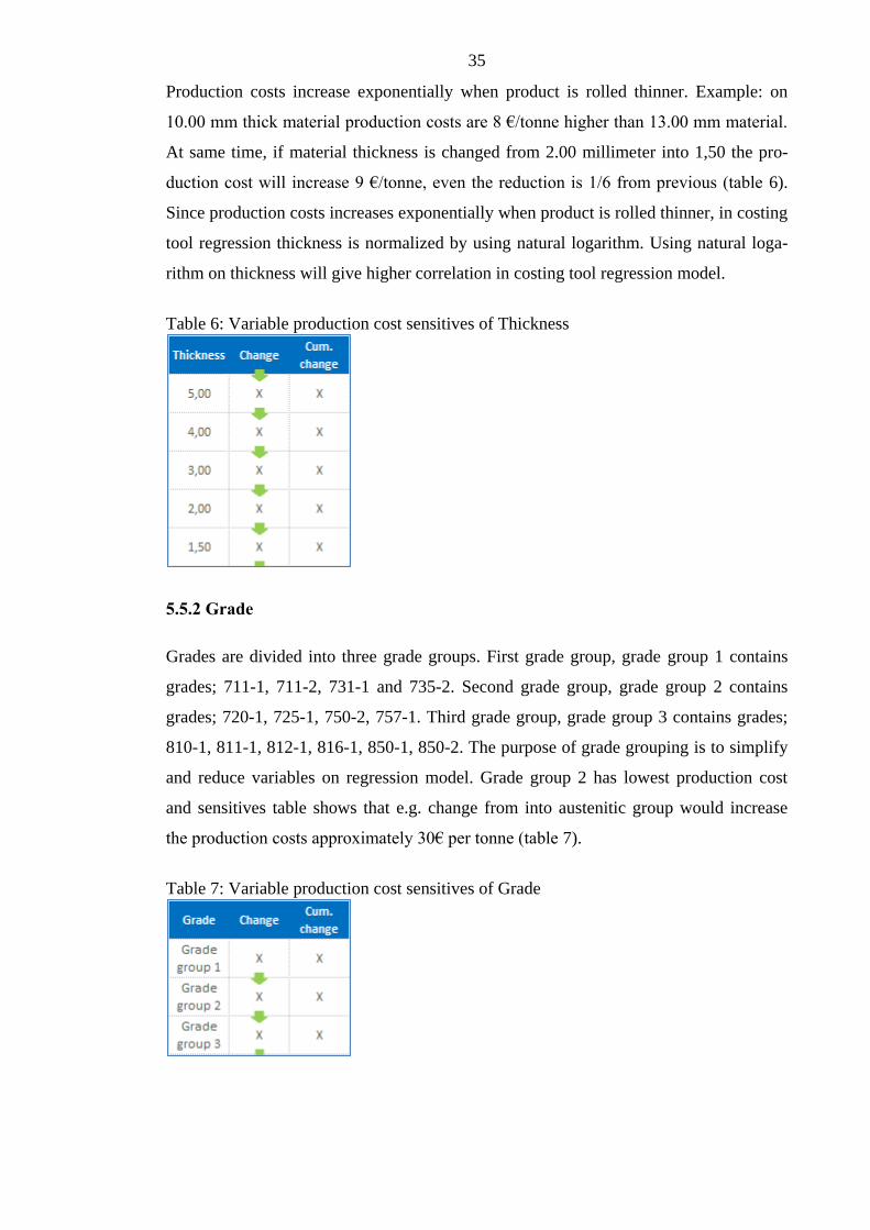
Production costs increase exponentially when product is rolled thinner. Example: on
10.00 mm thick material production costs are 8 €/tonne higher than 13.00 mm material.
At same time, if material thickness is changed from 2.00 millimeter into 1,50 the pro-
duction cost will increase 9 €/tonne, even the reduction is 1/6 from previous (table 6).
Since production costs increases exponentially when product is rolled thinner, in costing
tool regression thickness is normalized by using natural logarithm. Using natural loga-
rithm on thickness will give higher correlation in costing tool regression model.
Table 6: Variable production cost sensitives of Thickness
5.5.2 Grade
Grades are divided into three grade groups. First grade group, grade group 1 contains
grades; 711-1, 711-2, 731-1 and 735-2. Second grade group, grade group 2 contains
grades; 720-1, 725-1, 750-2, 757-1. Third grade group, grade group 3 contains grades;
810-1, 811-1, 812-1, 816-1, 850-1, 850-2. The purpose of grade grouping is to simplify
and reduce variables on regression model. Grade group 2 has lowest production cost
and sensitives table shows that e.g. change from into austenitic group would increase
the production costs approximately 30€ per tonne (table 7).
Table 7: Variable production cost sensitives of Grade
36
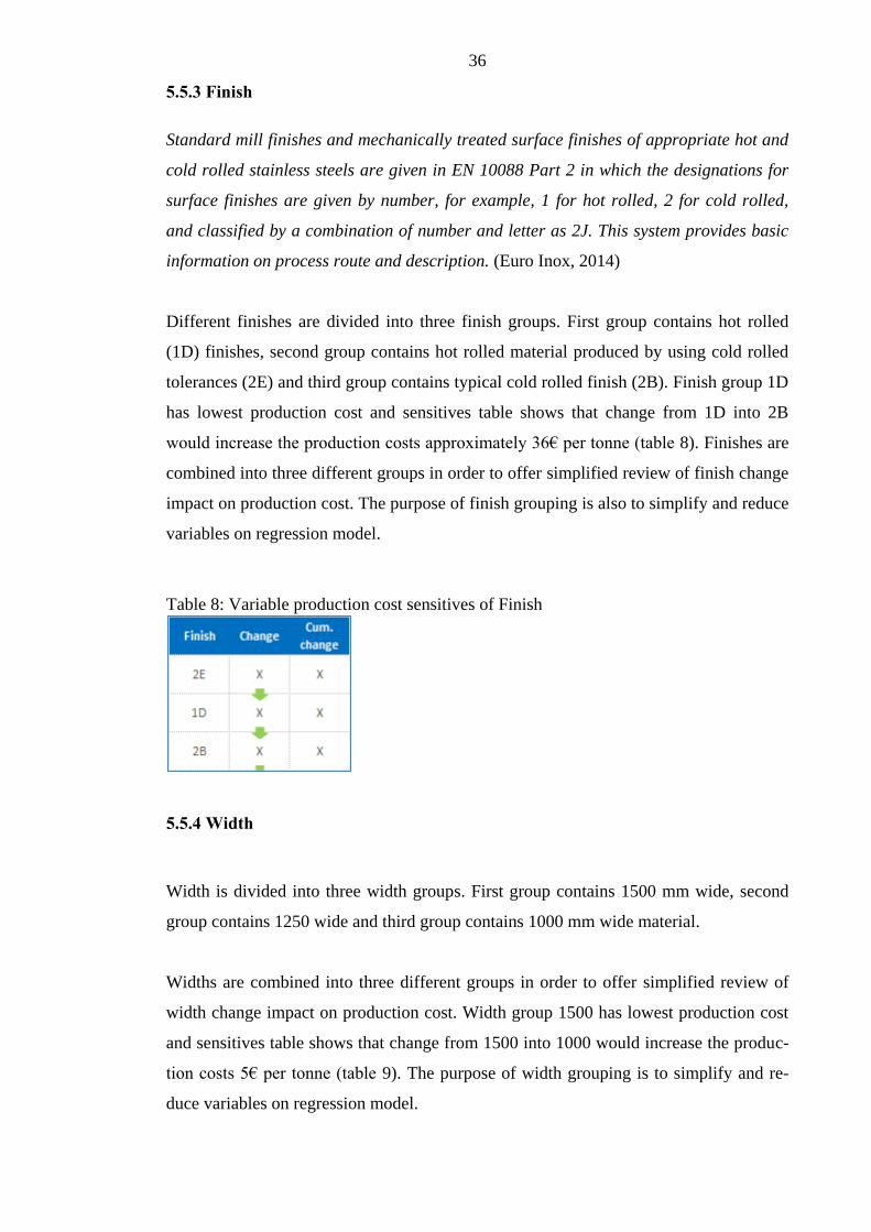
5.5.3 Finish
Standard mill finishes and mechanically treated surface finishes of appropriate hot and
cold rolled stainless steels are given in EN 10088 Part 2 in which the designations for
surface finishes are given by number, for example, 1 for hot rolled, 2 for cold rolled,
and classified by a combination of number and letter as 2J. This system provides basic
information on process route and description. (Euro Inox, 2014)
Different finishes are divided into three finish groups. First group contains hot rolled
(1D) finishes, second group contains hot rolled material produced by using cold rolled
tolerances (2E) and third group contains typical cold rolled finish (2B). Finish group 1D
has lowest production cost and sensitives table shows that change from 1D into 2B
would increase the production costs approximately 36€ per tonne (table 8). Finishes are
combined into three different groups in order to offer simplified review of finish change
impact on production cost. The purpose of finish grouping is also to simplify and reduce
variables on regression model.
Table 8: Variable production cost sensitives of Finish
5.5.4 Width
Width is divided into three width groups. First group contains 1500 mm wide, second
group contains 1250 wide and third group contains 1000 mm wide material.
Widths are combined into three different groups in order to offer simplified review of
width change impact on production cost. Width group 1500 has lowest production cost
and sensitives table shows that change from 1500 into 1000 would increase the produc-
tion costs 5€ per tonne (table 9). The purpose of width grouping is to simplify and re-
duce variables on regression model.

37
Table 9: Variable production cost sensitives of Width
5.5.5 Shape
Shape is divided into two shape groups. First group contains coil and second group con-
tains sheet material.
Shape is combined into two different groups in order to offer simplified review of shape
change impact on production cost. On shape group costing tool do not take account
length of material. Shape group coil has lowest production cost and sensitives table
shows that change from coil into sheet would increase the production costs 13€ per
tonne (table 10). The purpose of shape grouping is to simplify and reduce variables on
regression model.
Table 10: Variable production cost sensitives of Shape

38
5.5.6 Edge
Edge is divided into two edge groups. First group contains mill and second group con-
tains cut material.
Edge is combined into two different groups in order to offer simplified review of edge
change impact on production cost. Edge group mill has lowest production cost and sen-
sitives table shows that change from mill into cut would increase the production costs
10€ per tonne (table 11). The purpose of edge grouping is to simplify and reduce varia-
bles on regression model.
Table 11: Variable production cost sensitives of Edge
39
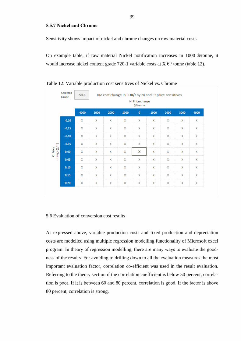
5.5.7 Nickel and Chrome
Sensitivity shows impact of nickel and chrome changes on raw material costs.
On example table, if raw material Nickel notification increases in 1000 $/tonne, it
would increase nickel content grade 720-1 variable costs at X € / tonne (table 12).
Table 12: Variable production cost sensitives of Nickel vs. Chrome
5.6 Evaluation of conversion cost results
As expressed above, variable production costs and fixed production and depreciation
costs are modelled using multiple regression modelling functionality of Microsoft excel
program. In theory of regression modelling, there are many ways to evaluate the good-
ness of the results. For avoiding to drilling down to all the evaluation measures the most
important evaluation factor, correlation co-efficient was used in the result evaluation.
Referring to the theory section if the correlation coefficient is below 50 percent, correla-
tion is poor. If it is between 60 and 80 percent, correlation is good. If the factor is above
80 percent, correlation is strong.
40
Obvious aim was to get costing tool conversion costs regression models correlation co-
efficient as high as possible. In variable regression model, 64 percent coefficient was
achieved. In the fixed and depreciation production costs, correlation coefficient was
higher at 73 percent.
As discussed above number of variables in regression model was restricted intentionally
in one hand to keep the model lean and understandable and on the other hand due to
limitations of Microsoft excel program. Accuracy of the model can be increased by add-
ing number of variables or cleaning the source data. Recommendation for further devel-
opment of the model is to improve validation process of the source data and understand-
ing of the regression model’s sensitiveness for deviant values. Potential areas of valida-
tion process improvement are automatizing of the source data checking or building the
data checks for the calculation process in order to avoid human or systematic errors. By
investigating the deviant values of the source data outliers can be recognized and further
analyzed is there natural reason for deviation of data.

41
5.7 Freight model
In the previous version of the costing tool freight costs were based on last known quar-
ter actual freights. The aim in the costing tool development was to apply agreed future
values of freights into costing tool. However, in meeting with Outokumpu Stainless Oy
logistics, we agreed that latest known actuals are continued to be used as freight values.
It was also agreed that new freight data evaluation process will be established. You can
find own chapter of the freight data evaluation from this thesis (chapter 6.4).
Outokumpu Stainless Oy logistics gave strong recommendation, that costing tool user
should not be able to select transport mode in the tool. According to them there is high
risk to misinterpret our freight cost by choosing e.g. lower cost container rather than
truck. Despite the recommendation it was decided that optional choice of transport
mode remains in the tool. Costing tool default choice, average cost of transport mode is
added as a default choice for tool. Additionally in the meeting with logistics was agreed
that optional choice of open top container needs to be applied into transport modes.
(Untinen & Knuuti & Pitko 2014)
42
6 UPDATE PROCESS
Update process of the current and developed costing tool is unchanged in principle.
However the documentation of the update process was updated. As previously costing
tool is updated and sent to end users regularly. Data for costing tool is updated accord-
ing to costing tool schedule.
6.1 Raw material and currency exchange rate update process
After raw material and currency exchange rate of USD has been updated, costing tool
administrator will review updated data and compare against previous weeks’ data, in
case there are possible update errors in data. If errors are not found, new raw material
data is replaced to the model. After costing tool is updated, administrator sends updated
costing tool for end users via e-mail. In the new version of the tool, both actions of raw
material updates and e-mail sending is automated, by using excel macros. E-mail is sent
to costing tool administrator, where then forwarded to end user.
6.2 Raw material cost model update
On agreed schedule costing tool raw material cost model needs to be updated. Costing
tool administrator will update melting shops scrap mixes and melting shops production
volume. This update is done by using structured query language (SQL) query and data
is picked up from Vertical Profitability System.
On agreed schedule basis, costing tool administrator will send request for raw material
purchasing and ask data for raw material prices in prime and scrap. Raw material pur-
chase person will collect, evaluate and reply data via e-mail back to costing tool admin-
istrator. On this development we agreed that costing tool updates of raw materials are
evaluated by raw material purchase.
43
6.3 Conversion cost model update
After vertical profitability closing process, costing tool administrator will update costing
tool variable, fixed and other costs regression data. Regression update is done by using
sql query and data is picked up from Vertical Profitability system.
Costing tool administrator will review updated data and compare it earlier data, if there
is possible update errors of data. If errors have not been founded, administrator will up-
date regressions into user version and then on next update of costing tool, these updated
regression data will be used.
6.4 Freight cost model update
Earlier costing tool freight data was taken from Outokumpu Stainless Oy local reporting
tool, where there was no agreed validation process to find whether the agreed periodical
freights were accurate for costing tool. On this development we agreed that administra-
tor or costing tool will follow freight data evaluation process.
Freight data will be updated into costing tool based on agreed schedule. Historical data
of freights will be used for coming period on costing tool freights. Data update process
starts, when administrator of costing tool will pull data from local reporting tool and
send it for Outokumpu Stainless Oy logistics. Data set sent to logistics contains freight
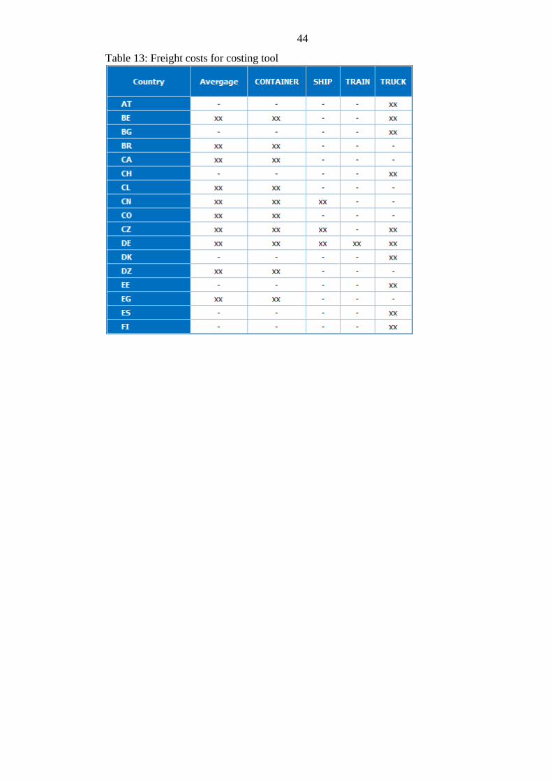
cost per transport mode and country (table 13). Costing tool administrator will compare
new freights for earlier freight data set and if he/she finds something curious, he/she
will send data for logistics together with finding(s) arguments. Otherwise if freight data
looks fine, costing tool administrator send data without any further comments.
Logistics will evaluate the received data and if they agree the data they reply and con-
firm data via e-mail. If logistics have a view of coming cost changes for coming period
(per transport mode, per country) on freights, they will correct the data and reply it back
for costing tool administrator within applied comments. This development will now
cover the freight data accuracy on costing tool and will take into account coming chang-
es on freights, which are evaluated and confirmed by best possible experts on company.
44
Table 13: Freight costs for costing tool
45
7 OTHER ACTIVITIES
Testing the tool started week 35/2014, when couple of test users started to test new cost-
ing tool. Costing tool tests continued, by updating new tool on parallel with first version
of the tool. During the first weeks, developed costing tool new regression, variable- and
fixed costs, raw material calculations, etc. were reviewed and compared against the first
version. This comparison was done, since there was need to validate and compare that
new tool will give accurate and obviously better results than the old one.
The tool testing was ended week 41/2014 and wider group of users was applied into tool
distribution. At the same time, when distribution was extended, communication and
introduction of new tool was given for end users.
Training material of the tool was built and all the existing and new items in the tool
were introduced in training material. Training of the tool was given to the end users by
using company remote communication system Lync.
At the beginning and obviously during the costing tool development, it has been self-
clear that this type of tools exists elsewhere in company than just in Tornio. One of the
similar types of costing tool used in Nirosta, was introduced for me during this devel-
opment. I also got the information, that in Outokumpu all the business units have their
own revision of pricing tool used for pricing.
This information raises an obvious question whether the company should start to har-
monize these types of tools and build one common for whole group. Since this devel-
opment was limited to review only Tornio tool, this thesis do not review any other busi-
ness line costing tools. However there already is a large project in Outokumpu, which
would then take even harmonization work of different type costing tools into account.
Another development request for costing tool point of view is current tool distribution
restrictions. Since agreement was to build also the new tool on excel basis, it generates
possible illegal use of the tool. In order to avoid any illegal use of this tool, there is a
development request to build access restriction for it. By applying user access for the
tool, system owner and administrator can guarantee that only permitted users are able to
use the tool.
46
8 SUMMARY
Development of costing tool reviewed tool end user selection criteria, applied optional
delivery months and changed delivery default type into average freight costs of deliver-
ies in selected country. Development extended costing tool result table profitability
view from contribution down to operating profit. Development applied also validity of
the tool, where end user could view for how long used tool is valid, or if tool is outdat-
ed.
In background, this development applied new regression calculation into conversion
cost model. New regression contains reviewed variable costs, new fixed cost regression
and sales and marketing, general and administration and other costs. These regression
calculation updates were not only done for cold rolled products, but also for semi mate-
rial for black hot bands. Raw material cost future values on raw material calculation
were applied. Raw material future values can give estimation of raw material costs for
next 62 months.
On development all the data input processes were reviewed and updated. Imported data
will be compared against earlier data and by using agreed business logic for data evalua-
tion, all the smallest possible errors would be found. By using developed data input re-
view, we lower the risk to use odd values on costing tool. Implemented comparison be-
tween latest update and earlier used data gives visibility of data set changes and support
update process to guarantee the good data validity for costing tool.
During this development, all the costing tool elements were evaluated documented and
their calculation and update process, source of values and validation were re-established
where needed. Costing tool development included also comparison and sensitivity anal-
ysis between earlier used data set vs. updated data set. Development of costing tool will
increase trustworthiness of used data sets and give reliable, accurate and timely correct
results for end user to agree stainless steel prices with customer.

47
9 CONTEMPLATION
To review and develop new costing tool for Outokumpu Stainless Oy was absolutely an
interesting and totally new area for me. As agreed in my earlier personal development
dialog, “think outside of box”, this work was reality of it. Obviously main reason to
start to develop this tool was my intention to build something useful for company. I
thought that even if it was demanding and hard to satisfy all the people around this top-
ic, it was worth of it.
At least in Finland we have the saying; a rolling stone gathers no moss, where I certain-
ly do not refer for one of the best rock n roll group in music history. Stepping out of
your own comfort zone gives new ideas about how you can improve your current work.
Secondly, it would be ideal to view your own work and company’s other functions with
“new” eyes.
Developing new costing tool for Outokumpu Stainless gave me real opportunity to learn
how company pricing works in practice and by writing those learnings into my school
thesis, I really hit two flies at once. Secondly, those students, who claim that they would
never need any mathematical learning in real life, please think twice. During my thesis I
learn how the multiple regression works, how regression data outliers need to be tackled
and how you need to take into account different cost element impact for end results, all
in mathematic model. If your intention is to build, develop, be involved in any sales or
financial management matters, learn math!
Last I can state that building this new costing tool to company, even if it has been very
busy and stressful time, it has been also absolutely great and satisfying time to complete
something new for own company.
48
LIST OF REFERENCES
Asish K. Bhattacharyya, Principles and Practice of Cost Accounting, 2004,
pages 288 – 299.
Davenport, T. & Harris, J. 2007. Competing on Analytics.
Harvard Business School Publishing.
Euro Inox, The European Stainless Steel Development Association, euro-inox.org,
retrieval date 17th
of Sep 2014.
European Central Bank, www.ecb.europa.eu, retrieval date 3rd
of April 2014.
London Metal Exchange, LME. www.lme.com, retrieval date 22nd
of June 2014.
Metal Bulletin, MB. www.metalbulleting.com, retrieval date 18th
of June 2014.
Michael V. Marn, Eric V. Roegner, and Craig C. Zawada. McKinsey&Company,
The power of pricing. February 2003
http://www.mckinsey.com/insights/marketing_sales/the_power_of_pricing,
retrieval date 7th
of October 2014.
Montgomery, D., Peck, E. & Vining, G, 2012. An Introduction to Linear Regression
Analysis, pages 12 – 21 and 67 – 74.
Outokumpu Intranet, 2014. Retrieval date 29th
of October 2014.
Thomas J. Archdeacon, Correlation and Regression Analysis:
A Historian's Guide, 1994, Pages 98 -99.
Untinen, T., Knuuti, J. & Pitko Pertti, 2014 Outokumpu Stainless Oy, meeting at 23rd
of June 2014.