Development of Benthic Community Condition … 735 NOV 2014 Development of Benthic Community Condition Indices – San Francisco Bay Contract#: 1038 Phase I Final Report November 26,

NUMBER

735

NOV2014

Development of Benthic Community Condition Indices – San Francisco BayContract#: 1038

Phase I Final Report

November 26, 2014

By:

David J. Gillett

J. Ananda Ranasinghe

Eric D. Stein

Southern California Coastal Water Research Project

CLEAN WATER / RMP

S A N F R A N C I S C O E S T U A RY I N S T I T U T E 4911 Central Avenue, Richmond, CA 94804 • p: 510-746-7334 (SFEI) • f: 510-746-7300 • www.sfei.org

THIS REPORT SHOULD BE CITED AS:

Gillett, D. J., Ranasinghe, J. A., Stein, E. D. (2014). RMP 2012 Special Study. Development of Benthic Community Condition Indices – San Francisco Bay. Phase I Final Report. Contract#: 1038. San Francisco Estuary Institute, Richmond. CA. Contribution # 735.

1

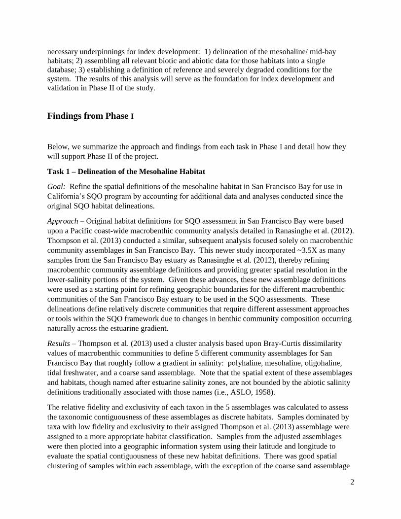
Introduction

Benthic community assessment is often used as an indicator of ecosystem condition and has

become a central element of regulatory programs such as the California’s sediment quality

objectives (SQO) for bays and estuaries. Benthos are the indicators of choice for monitoring and

assessment for several reasons, including:

Limited mobility makes them reflective of impacts at the site where they are collected.

Several animal phyla and classes are sensitive to impacts to their environments and can

be used to differentiate certain types of effects.

Life-histories are short enough that the effects of one-time impacts disappear within a

year but long enough to integrate the effects of multiple impacts occurring within

seasonal time scales.

Living in the bottom sediments, benthos have high exposure to common anthropogenic

impacts, such as sediment contamination, high sediment organic carbon, and low

bottom dissolved oxygen.

They are important components of aquatic food webs, transferring carbon and nutrients

from suspended particulates in the water column to the sediments by filter feeding and

serving as forage for bottom-feeding fishes.

For benthic data to be useful in a regulatory context, they must be synthesized into some manner

of index that can be interpreted in relation to scientifically valid criteria or thresholds that

distinguish “healthy” from “unhealthy” benthic communities. While reducing complex

biological data to index values has disadvantages, the resulting indices remove much of the

subjectivity associated with ad hoc data interpretation. Such indices also provide a simple means

of communicating complex information to managers, tracking trends over time, and correlating

benthic responses with stressor data.

To date, benthic indices have been calibrated and validated for two nearshore habitats in

California, 1) southern California marine bays, and 2) polyhaline (high salinity) portions of San

Francisco Bay. Indices have not yet been developed for other habitats throughout the State due

to a lack of sufficient calibration/validation data, compounded by a poorer understanding of

benthic community stressor-response relationships in lower salinity or naturally disturbed

habitats. The lower salinity portions of estuaries are particularly challenging because they are

subject to relatively broad ranges of natural environmental conditions (e.g., salinity, dissolved

oxygen, turbidity), which produces an endemic fauna adapted to tolerate environmental (and

possibly anthropogenic) stress. These challenges for assessment can, however, be overcome

through compilation of robust data sets and careful identification of reference conditions to

anchor indices.

With the long-term goal of developing a benthic index for the mesohaline/ North and South Bay

portions of San Francisco Bay, the objective of Phase I of this study was to provide the following

2

necessary underpinnings for index development: 1) delineation of the mesohaline/ mid-bay

habitats; 2) assembling all relevant biotic and abiotic data for those habitats into a single

database; 3) establishing a definition of reference and severely degraded conditions for the

system. The results of this analysis will serve as the foundation for index development and

validation in Phase II of the study.

Findings from Phase I

Below, we summarize the approach and findings from each task in Phase I and detail how they

will support Phase II of the project.

Task 1 – Delineation of the Mesohaline Habitat

Goal: Refine the spatial definitions of the mesohaline habitat in San Francisco Bay for use in

California’s SQO program by accounting for additional data and analyses conducted since the

original SQO habitat delineations.

Approach – Original habitat definitions for SQO assessment in San Francisco Bay were based

upon a Pacific coast-wide macrobenthic community analysis detailed in Ranasinghe et al. (2012).

Thompson et al. (2013) conducted a similar, subsequent analysis focused solely on macrobenthic

community assemblages in San Francisco Bay. This newer study incorporated ~3.5X as many

samples from the San Francisco Bay estuary as Ranasinghe et al. (2012), thereby refining

macrobenthic community assemblage definitions and providing greater spatial resolution in the

lower-salinity portions of the system. Given these advances, these new assemblage definitions

were used as a starting point for refining geographic boundaries for the different macrobenthic

communities of the San Francisco Bay estuary to be used in the SQO assessments. These

delineations define relatively discrete communities that require different assessment approaches

or tools within the SQO framework due to changes in benthic community composition occurring

naturally across the estuarine gradient.

Results – Thompson et al. (2013) used a cluster analysis based upon Bray-Curtis dissimilarity

values of macrobenthic communities to define 5 different community assemblages for San

Francisco Bay that roughly follow a gradient in salinity: polyhaline, mesohaline, oligohaline,

tidal freshwater, and a coarse sand assemblage. Note that the spatial extent of these assemblages

and habitats, though named after estuarine salinity zones, are not bounded by the abiotic salinity

definitions traditionally associated with those names (i.e., ASLO, 1958).

The relative fidelity and exclusivity of each taxon in the 5 assemblages was calculated to assess

the taxonomic contiguousness of these assemblages as discrete habitats. Samples dominated by

taxa with low fidelity and exclusivity to their assigned Thompson et al. (2013) assemblage were

assigned to a more appropriate habitat classification. Samples from the adjusted assemblages

were then plotted into a geographic information system using their latitude and longitude to

evaluate the spatial contiguousness of these new habitat definitions. There was good spatial

clustering of samples within each assemblage, with the exception of the coarse sand assemblage

3

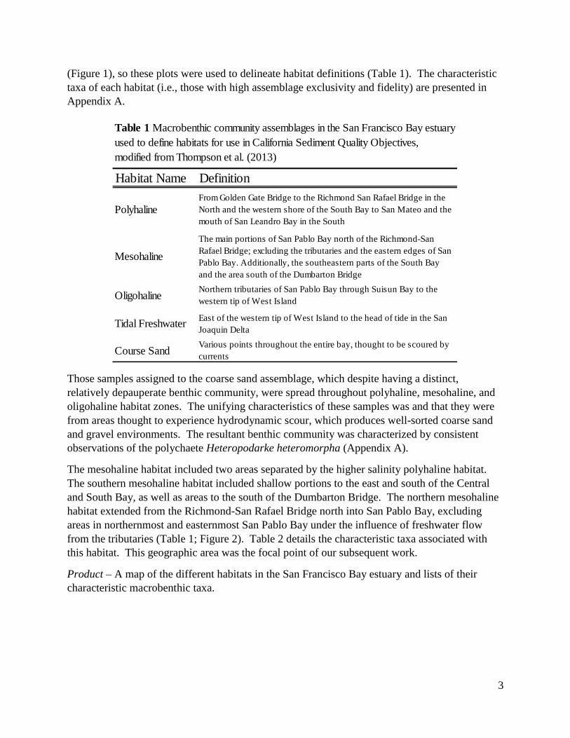
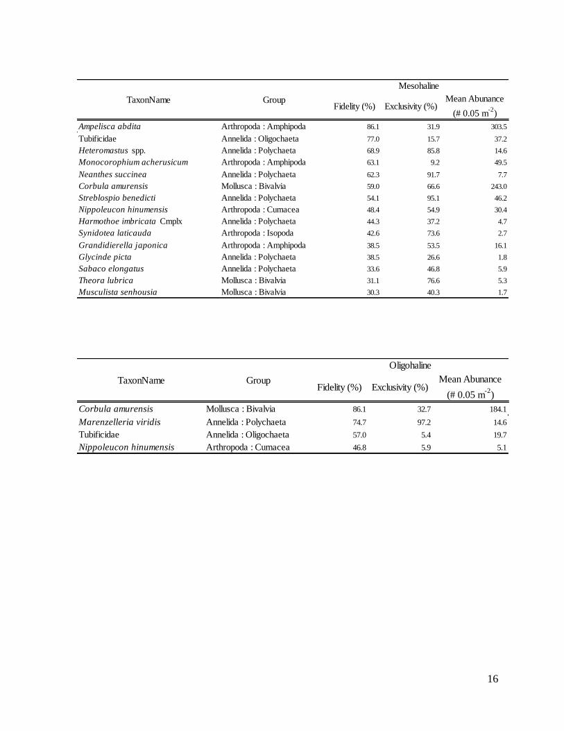
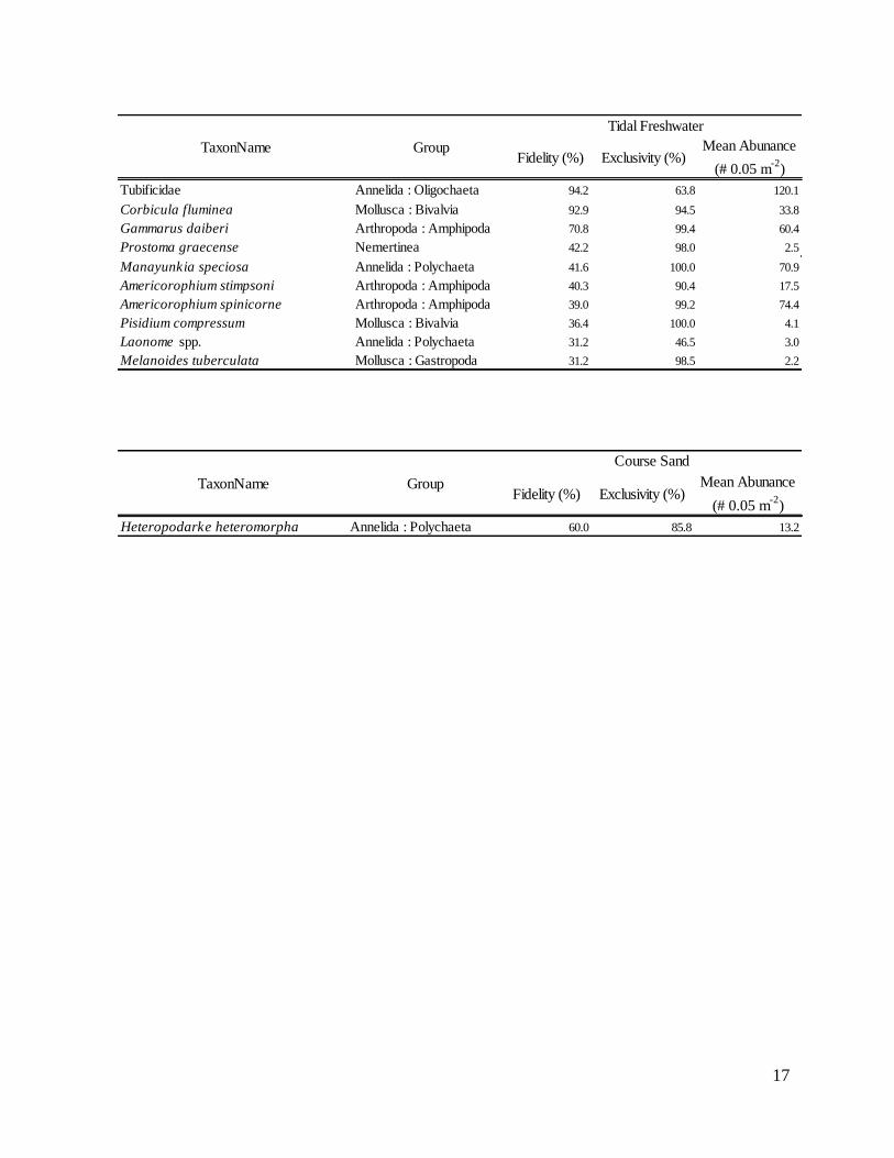
(Figure 1), so these plots were used to delineate habitat definitions (Table 1). The characteristic

taxa of each habitat (i.e., those with high assemblage exclusivity and fidelity) are presented in

Appendix A.

Those samples assigned to the coarse sand assemblage, which despite having a distinct,

relatively depauperate benthic community, were spread throughout polyhaline, mesohaline, and

oligohaline habitat zones. The unifying characteristics of these samples was and that they were

from areas thought to experience hydrodynamic scour, which produces well-sorted coarse sand

and gravel environments. The resultant benthic community was characterized by consistent

observations of the polychaete Heteropodarke heteromorpha (Appendix A).

The mesohaline habitat included two areas separated by the higher salinity polyhaline habitat.

The southern mesohaline habitat included shallow portions to the east and south of the Central

and South Bay, as well as areas to the south of the Dumbarton Bridge. The northern mesohaline

habitat extended from the Richmond-San Rafael Bridge north into San Pablo Bay, excluding

areas in northernmost and easternmost San Pablo Bay under the influence of freshwater flow

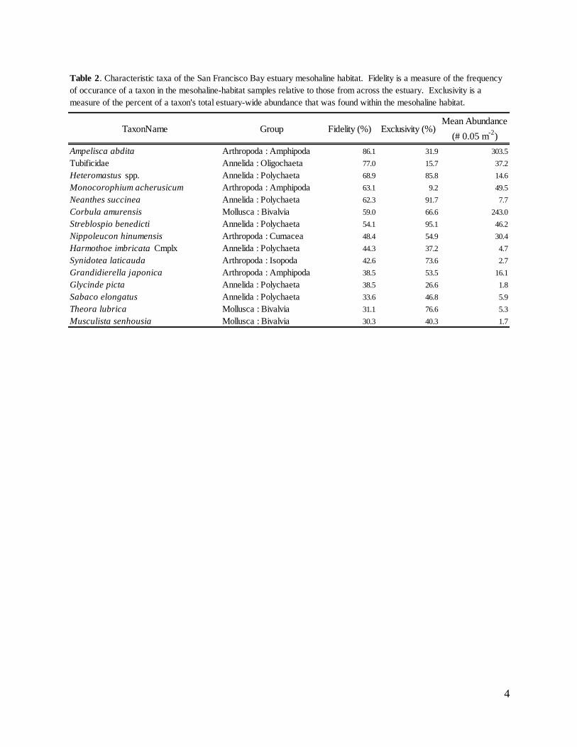
from the tributaries (Table 1; Figure 2). Table 2 details the characteristic taxa associated with

this habitat. This geographic area was the focal point of our subsequent work.

Product – A map of the different habitats in the San Francisco Bay estuary and lists of their

characteristic macrobenthic taxa.

Habitat Name Definition

PolyhalineFrom Golden Gate Bridge to the Richmond San Rafael Bridge in the

North and the western shore of the South Bay to San Mateo and the

mouth of San Leandro Bay in the South

Mesohaline

The main portions of San Pablo Bay north of the Richmond-San

Rafael Bridge; excluding the tributaries and the eastern edges of San

Pablo Bay. Additionally, the southeastern parts of the South Bay

and the area south of the Dumbarton Bridge

OligohalineNorthern tributaries of San Pablo Bay through Suisun Bay to the

western tip of West Island

Tidal FreshwaterEast of the western tip of West Island to the head of tide in the San

Joaquin Delta

Course SandVarious points throughout the entire bay, thought to be scoured by

currents

Table 1 Macrobenthic community assemblages in the San Francisco Bay estuary

used to define habitats for use in California Sediment Quality Objectives,

modified from Thompson et al. (2013)

4

TaxonName Group Fidelity (%) Exclusivity (%)Mean Abundance

(# 0.05 m-2

)

Ampelisca abdita Arthropoda : Amphipoda 86.1 31.9 303.5

Tubificidae Annelida : Oligochaeta 77.0 15.7 37.2

Heteromastus spp. Annelida : Polychaeta 68.9 85.8 14.6

Monocorophium acherusicum Arthropoda : Amphipoda 63.1 9.2 49.5

Neanthes succinea Annelida : Polychaeta 62.3 91.7 7.7

Corbula amurensis Mollusca : Bivalvia 59.0 66.6 243.0

Streblospio benedicti Annelida : Polychaeta 54.1 95.1 46.2

Nippoleucon hinumensis Arthropoda : Cumacea 48.4 54.9 30.4

Harmothoe imbricata Cmplx Annelida : Polychaeta 44.3 37.2 4.7

Synidotea laticauda Arthropoda : Isopoda 42.6 73.6 2.7

Grandidierella japonica Arthropoda : Amphipoda 38.5 53.5 16.1

Glycinde picta Annelida : Polychaeta 38.5 26.6 1.8

Sabaco elongatus Annelida : Polychaeta 33.6 46.8 5.9

Theora lubrica Mollusca : Bivalvia 31.1 76.6 5.3

Musculista senhousia Mollusca : Bivalvia 30.3 40.3 1.7

Table 2. Characteristic taxa of the San Francisco Bay estuary mesohaline habitat. Fidelity is a measure of the frequency

of occurance of a taxon in the mesohaline-habitat samples relative to those from across the estuary. Exclusivity is a

measure of the percent of a taxon's total estuary-wide abundance that was found within the mesohaline habitat.

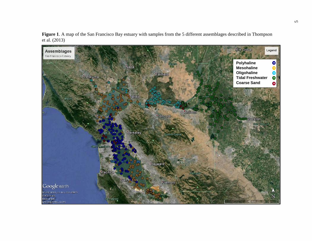
Figure 1. A map of the San Francisco Bay estuary with samples from the 5 different assemblages described in Thompson

et al. (2013)

Polyhaline

Mesohaline

Oligohaline

Tidal Freshwater

Coarse Sand

5

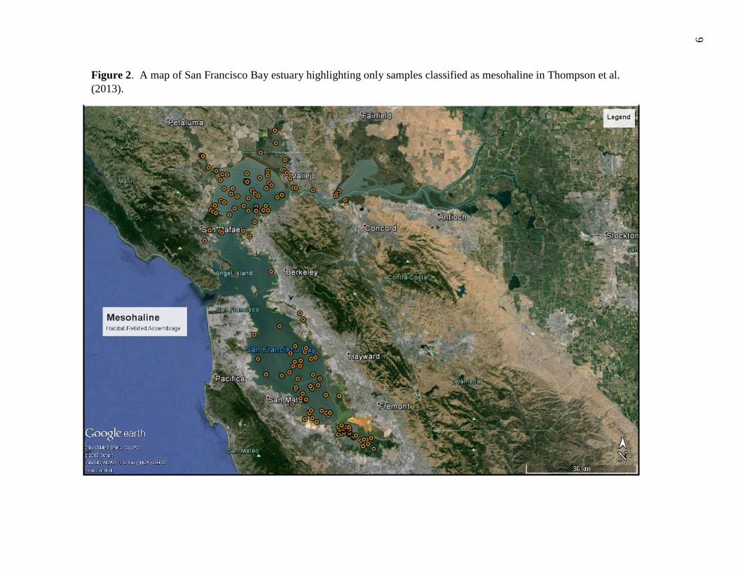
Figure 2. A map of San Francisco Bay estuary highlighting only samples classified as mesohaline in Thompson et al.

(2013).

6

7

Task 2 – Data Assembly and Standardization

Goal – To assemble all of the available biology, environmental, and stressor data available for

the San Francisco Bay estuary that would be used in developing a macrobenthic community

assessment tool(s) into a single relational database.

Approach – Macrobenthic abundance and environmental data (e.g., habitat, contaminant,

toxicity) from all available San Francisco Bay benthic sampling efforts were aggregated into a

single relational database. As these data were from a variety of sampling programs that used

different types of sampling gear and taxonomic standards, the data had to be transformed and

updated to create a uniform, comparable standard across all samples. Additionally, all samples

were assigned to their appropriate new habitat classification so that they could be used in this and

future SQO-related work.

Results – Data from 6,857 benthic samples collected during 2,336 sampling events at 486

different sites across all habitat types were compiled. These data came from 11 different

sampling programs and were collected from 1992 to 2012 (see database for details). Some

combinations of depth, sediment composition, or salinity data were available for 2,068 of those

sampling events. Sediment contaminant data were available for only 236 sampling events.

Sediment toxicity test data, typically amphipod survival tests, were available for 159 sampling

events.

Within the mesohaline habitat described under Task 1, data were available from 1,361 benthic

samples from 497 sampling events at 141 different sites. Depth, sediment composition, or

salinity data were available for 497 sampling events. Sediment contaminant data were available

for 83 sampling events and sediment toxicity data were available for 68 sampling events.

As noted above, these data from across the entire estuary were collected by a number of different

sampling programs across two decades. Two byproducts of this are that 1) different sediment

grabs with different surface areas were used; and 2) the taxonomic level (e.g., subclass vs.

species for oligochaetes) and taxonomic standards (e.g., Dorvillea annulata vs. Schistomeringos

annulata) varied across years. The largest sediment grab used was a 0.05-m2 ponar grab, so all

abundance data were standardized to # individuals per 0.05 m-2. Taxon names were standardized

to Southern California Association of Marine Taxonomists species list Edition 6 (SCAMIT

2011).

There were detectable differences in species richness across the different types of gear used for

collecting samples, with samples taken with larger gear having more species; this problem is not

as easily correctable as the abundance differences. However, the differences in species richness

among gear types were not uniform along the salinity gradient. The most pronounced effects

were in the higher-diversity polyhaline habitats; there were smaller differences in the

mesohaline, and no differences among gear types in the oligohaline or tidal freshwater portions

of the estuary. As a consequence, care will have to be taken in selection of data for use in the

creation of any subsequent assessment index, especially those using species richness/diversity or

the presence/absence of rare taxa.

8

Product – MS Access database of benthic, environmental, and toxicity data

Task 3 - Establishing a Definition of Reference and Degraded Conditions

Goal – Use expert knowledge of benthic ecology in lower-salinity estuarine ecosystems to create

definitions of reference and degraded macrobenthic communities that can then be used to

develop and validate benthic condition indices for use in SQO assessments.

Approach – A clear definition of reference condition is one the first key steps in developing a

habitat assessment tool (Stoddard et al. 2006; Muxika et al. 2007; Hawkins et al. 2010).

Understanding the reference condition anchors expectations when evaluating novel sites; doing

so makes it possible to determine how different samples are from reference and potentially to

chart a path towards recovery to that state. There are a variety of ways to set reference

expectations for a system (e.g., Hughes et al. 1986; Reynoldson et al. 1997; Ranasinghe et al.

2009), but given the lack of proven conceptual models and the associated difficulty in defining

reference conditions in integrative and transitional habitats like estuaries in general, and San

Francisco Bay in particular, we chose to develop reference/degraded definitions using the

knowledge of experienced benthic ecologists. A panel of nine expert benthic ecologists with

experience in lower-salinity estuaries and/or San Francisco Bay was assembled to evaluate the

condition of macrobenthic community samples. The experts were asked to evaluate the

condition of 30 benthic samples from the mesohaline habitat that were selected from along

gradients of habitat quality (e.g., sediment contaminants, sediment toxicity, and community

parameters).

The expert panel members were given only information on benthic community composition (taxa

names and abundance) and environmental characteristics (depth, sediment composition, and

salinity) where available. They were not given information on sample location, sediment

contaminants, or sediment toxicity. The experts were asked to assign samples into 1 of 4

condition categories – undisturbed through severely degraded – and rank all of the samples from

best to worst.

9

Sample ID Expert 1 Expert 2 Expert 3 Expert 4 Expert 5 Expert 6

Mesohaline Sample 1 3 2 2 1 3 2






























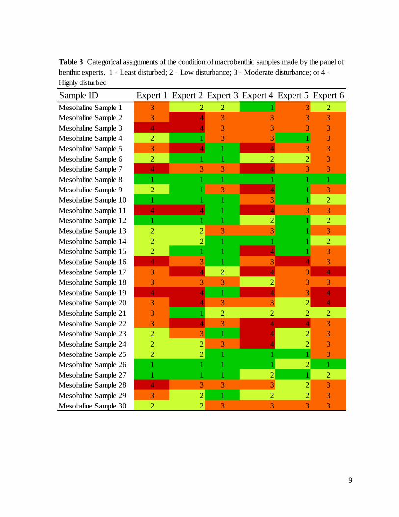
Table 3 Categorical assignments of the condition of macrobenthic samples made by the panel of

benthic experts. 1 - Least disturbed; 2 - Low disturbance; 3 - Moderate disturbance; or 4 -

Highly disturbed

10

Sample ID Expert 1 Expert 2 Expert 3 Expert 4 Expert 5 Expert 6

Mesohaline Sample 1 24 11 18 4.5 19.5 4.5

Mesohaline Sample 2 21 28 29 18 26.0 23.5

Mesohaline Sample 3 29 26 20.5 16 19.5 23.5

Mesohaline Sample 4 12 10 25 18 5.5 17



Mesohaline Sample 7 28 20 26.5 26.5 22.0 23.5






Mesohaline Sample 13 8 15 20.5 13 5.5 11.5







Mesohaline Sample 20 18 24 26.5 18 13.0 29








Mesohaline Sample 28 26 21 29 14.5 15.0 17



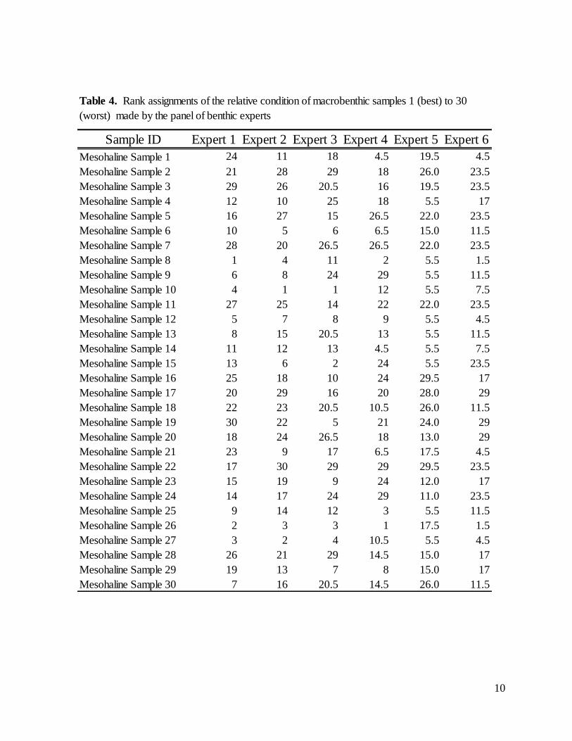
Table 4. Rank assignments of the relative condition of macrobenthic samples 1 (best) to 30

(worst) made by the panel of benthic experts

11

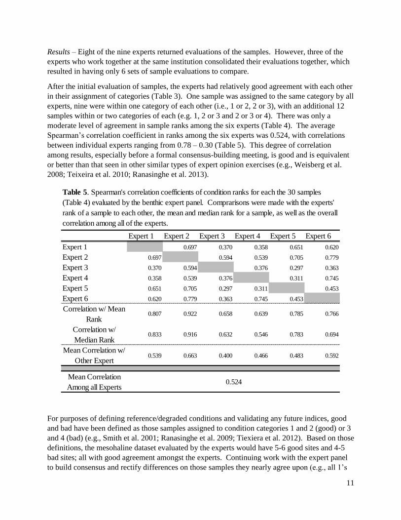
Results – Eight of the nine experts returned evaluations of the samples. However, three of the

experts who work together at the same institution consolidated their evaluations together, which

resulted in having only 6 sets of sample evaluations to compare.

After the initial evaluation of samples, the experts had relatively good agreement with each other

in their assignment of categories (Table 3). One sample was assigned to the same category by all

experts, nine were within one category of each other (i.e., 1 or 2, 2 or 3), with an additional 12

samples within or two categories of each (e.g. 1, 2 or 3 and 2 or 3 or 4). There was only a

moderate level of agreement in sample ranks among the six experts (Table 4). The average

Spearman’s correlation coefficient in ranks among the six experts was 0.524, with correlations

between individual experts ranging from 0.78 – 0.30 (Table 5). This degree of correlation

among results, especially before a formal consensus-building meeting, is good and is equivalent

or better than that seen in other similar types of expert opinion exercises (e.g., Weisberg et al.

2008; Teixeira et al. 2010; Ranasinghe et al. 2013).

For purposes of defining reference/degraded conditions and validating any future indices, good

and bad have been defined as those samples assigned to condition categories 1 and 2 (good) or 3

and 4 (bad) (e.g., Smith et al. 2001; Ranasinghe et al. 2009; Tiexiera et al. 2012). Based on those

definitions, the mesohaline dataset evaluated by the experts would have 5-6 good sites and 4-5

bad sites; all with good agreement amongst the experts. Continuing work with the expert panel

to build consensus and rectify differences on those samples they nearly agree upon (e.g., all 1’s

Expert 1 Expert 2 Expert 3 Expert 4 Expert 5 Expert 6

Expert 1 0.697 0.370 0.358 0.651 0.620

Expert 2 0.697 0.594 0.539 0.705 0.779

Expert 3 0.370 0.594 0.376 0.297 0.363

Expert 4 0.358 0.539 0.376 0.311 0.745

Expert 5 0.651 0.705 0.297 0.311 0.453

Expert 6 0.620 0.779 0.363 0.745 0.453

Correlation w/ Mean

Rank0.807 0.922 0.658 0.639 0.785 0.766

Correlation w/

Median Rank0.833 0.916 0.632 0.546 0.783 0.694

Mean Correlation w/

Other Expert0.539 0.663 0.400 0.466 0.483 0.592

Mean Correlation

Among all Experts0.524

Table 5. Spearman's correlation coefficients of condition ranks for each the 30 samples

(Table 4) evaluated by the benthic expert panel. Comprarisons were made with the experts'

rank of a sample to each other, the mean and median rank for a sample, as well as the overall

correlation among all of the experts.

12

and 2’s, with one 3) will likely increase the number of good and bad validation sites available for

future use.

In describing their evaluation process, all of the experts used some combination of abundance,

diversity, dominance, and their perceptions of the component taxa’s tolerance or sensitivity to

disturbance. Experts 2, 3, 4, and 6 focused primarily on whole community metrics like species

richness, diversity, and evenness to rank and organize sites and then used species composition

information to refine their sample order. Conversely, experts 1 and 5 relied more on their

perceptions of the tolerance, sensitivity and natural history of the fauna to inform their

evaluations, especially the relative abundance of stress-sensitive or tolerant taxa in a given

sample. This kind of information will be used in helping to craft assessment tools for the

mesohaline portions of San Francisco Bay.

Summary

With the completion of Phase I, the ground work to create a robust macrobenthos-based

assessment tool for use in California’s SQO framework in mesohaline San Francisco Bay is

completed. The habitat (i.e., the San Francisco Bay mesohaline community) has been

geographically delimited, data for the calibration and validation of an index have been

aggregated, and reference/degraded conditions have been reasonably well defined. The next step

in this process will be the development of a tool to assess the condition of the macrobenthic

community that is responsive to anthropogenic disturbance and accounts for the natural gradients

of mesohaline estuarine systems.

13

Literature Cited

ASLO. 1958. The Venice system for the classification of marine waters according to salinity.

Limnology and Oceanography 3: 346-347.

Hawkins, C.P. J.R. Olson, and R.A. Hill. 2010. The Reference Condition: Predicting benchmarks

for ecological water-quality assessments. Journal of the North American Benthological

Society 29: 312-343.

Hughes, R.M., D.P. Larsen, and J.M. Omernik. 1986. Regional reference sites: A method for

assessing stream potentials. Environmental Management 10: 629-635.

Muxika, I, A. Borja, and J. Bald. 2007. Using historical data, expert judgement and multivariate

analysis in assessing reference conditions and benthic ecological status, according to the

European Water Framework Directive. Marine Pollution Bulletin 55: 16-29.

Ranasinghe, J.A., S.B. Weisberg, R.W. Smith, D.E. Montagne, B. Thompson, J.M. Oakden, D.D.

Huff, D.B. Cadien, R.G. Velarde, and K.J. Ritter. 2009. Calibration and evaluation of five

indicators of benthic community condition in two California bay and estuary habitats.

Marine Pollution Bulletin 59: 5-13.

Ranasinghe, J.A., K.I Welch, P.N. Slattery, D.E. Montagne, D.D. Huff, H. Lee II, J.L. Hyland,

B. Thompson, S.B. Weisberg, J.M. Oakden, D.B. Cadien, and R.G. Velarde. 2012. Habitat-

related benthic macrofaunal assemblages of bays and estuaries of the western United States.

Integrated Environmental Assessment and Management 8: 638-648.

Ranasinghe, J.A., E.D. Stein, M.R. Frazier, and D.J. Gillett. 2013. Development of Puget Sound

Benthic Indicators. Southern California Coastal Water Research Project Technical Report

755. 63p. Costa Mesa, CA.

Reynoldson, T.B., R.H. Norris, V.H. Resh, K.E. Day, and D.M. Rosenberg. 1997. The reference

condition: A comparison of multimetric and multivariate approaches to assess water quality

impairment using benthic macroinvertebrates. Journal of the North American Benthological

Society 16: 833-852.

SCAMIT. 2011. A Taxonomic Listing of Benthic Macro- and Megainvertebrates. Edition 6.

Prepared by the Southern California Association of Marine Invertebrate Taxonomists, Los

Angeles, CA.

Smith, R.W., M. Bergen, S.B. Weisberg, D. Cadien, A. Dalkey, D. Montagne, J.K., Stull, and

R.G. Velarde. 2001. Benthic response index for assessing infaunal communities on the

Southern California mainland shelf. Ecological Applications 11: 1073-1087.

Stoddard, J.L., D.P. Larsen, C.P. Hawkins, R.K. Johnson, and R.H. Norris. 2006. Setting

expectations for the ecological condition of streams: the concept of reference condition.

Ecological Applications 16: 1267-1276.

14

Teixeira, H., A. Borja, S.B. Weisberg, J.A. Ranasinghe, D.B. Cadien, D.M. Dauer, J. Dauvin, S.

Degraer, R.J. Diaz, A. Grémare, I. Karakassis, R.J. Llansó, L.L. Lovell, J.C. Marques, D.E.

Montagne, A. Occhipinti-Ambrogi, R. Rosenberg, R. Sarda, L.C. Schaffner, and R.G.

Velarde. 2010. Assessing coastal benthic macrofauna community condition using best

professional judgement – Developing consensus across North America and Europe. Marine

Pollution Bulletin 60: 589-600.

Teixeira, H., S.B. Weisberg, A. Borja, J.A. Ranasinghe, D.B. Cadien, R.G. Velarde, L.L. Lovell,

D. Pasko, C.A. Phillips, D.E. Montagne, K.J. Ritter, F. Salas, and J.C. Marques. 2012.

Calibration and validation of the AZTI’s Marine Biotic Index (AMBI) for Southern

California marine bays. Ecological Indicators 12: 84-95.

Thompson, B., J.A. Ranasinghe, S. Lowe, A. Melwani, and S.B. Weisberg. 2013. Benthic

macrofaunal assemblages of the San Francisco Estuary and Delta. pp 163-176. In Southern

California Coastal Water Research Project Annual Report, K. Schiff (ed). Costa Mesa, CA.

Weisberg, S.B., B. Thompson, J.A. Ranasinghe, D.E. Montagne, D.B. Cadien, D.M. Dauer, D.

Diener, J. Oliver, D.J. Reish, R.G. Velarde, and J.W. Word. 2008. The level of agreement

among experts applying best professional judgement to assess the condition of benthic

infaunal communities. Ecological Indicators 8:389-394.

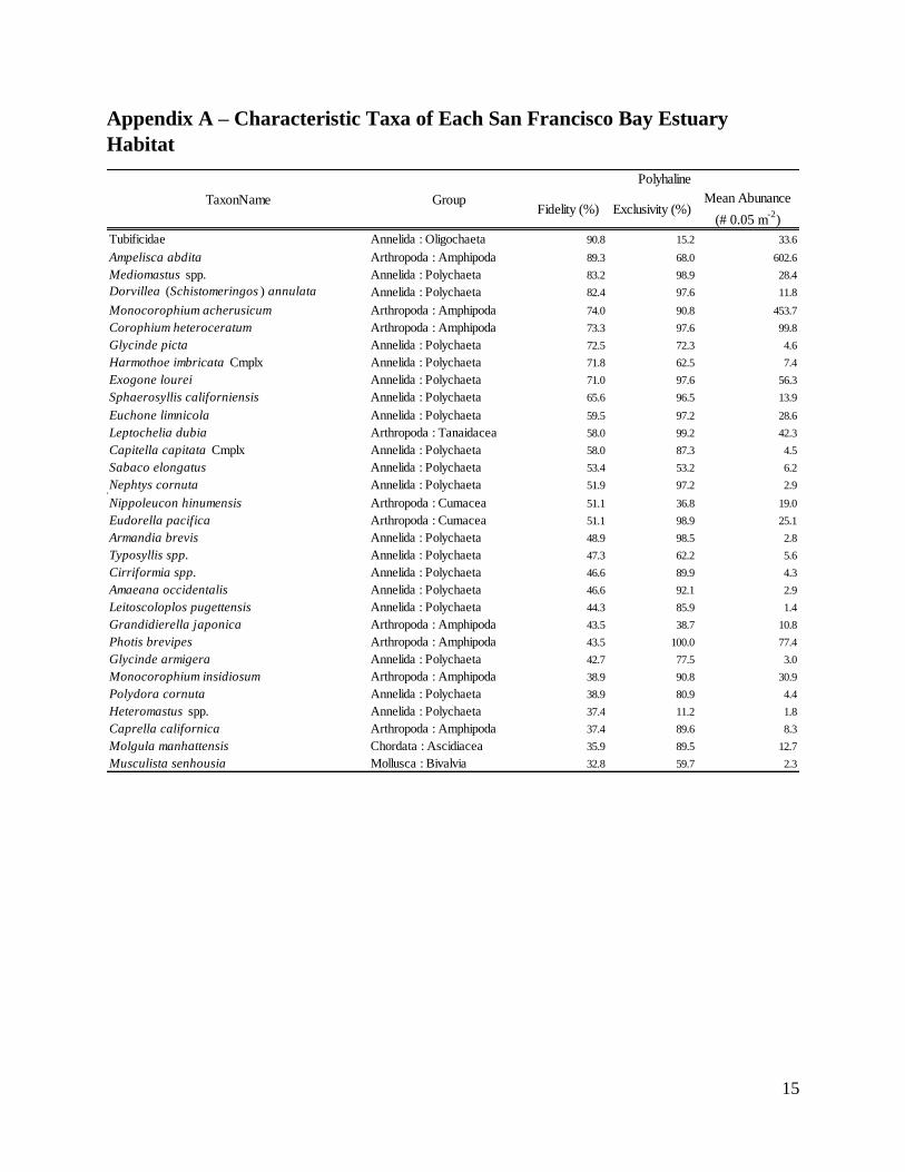
15

Appendix A – Characteristic Taxa of Each San Francisco Bay Estuary

Habitat

Fidelity (%) Exclusivity (%)Mean Abunance

(# 0.05 m-2

)



Mediomastus spp. Annelida : Polychaeta 83.2 98.9 28.4

Dorvillea (Schistomeringos ) annulata Annelida : Polychaeta 82.4 97.6 11.8


Corophium heteroceratum Arthropoda : Amphipoda 73.3 97.6 99.8



Exogone lourei Annelida : Polychaeta 71.0 97.6 56.3

Sphaerosyllis californiensis Annelida : Polychaeta 65.6 96.5 13.9

Euchone limnicola Annelida : Polychaeta 59.5 97.2 28.6

Leptochelia dubia Arthropoda : Tanaidacea 58.0 99.2 42.3

Capitella capitata Cmplx Annelida : Polychaeta 58.0 87.3 4.5


Nephtys cornuta Annelida : Polychaeta 51.9 97.2 2.9


Eudorella pacifica Arthropoda : Cumacea 51.1 98.9 25.1

Armandia brevis Annelida : Polychaeta 48.9 98.5 2.8

Typosyllis spp. Annelida : Polychaeta 47.3 62.2 5.6

Cirriformia spp. Annelida : Polychaeta 46.6 89.9 4.3

Amaeana occidentalis Annelida : Polychaeta 46.6 92.1 2.9

Leitoscoloplos pugettensis Annelida : Polychaeta 44.3 85.9 1.4


Photis brevipes Arthropoda : Amphipoda 43.5 100.0 77.4

Glycinde armigera Annelida : Polychaeta 42.7 77.5 3.0

Monocorophium insidiosum Arthropoda : Amphipoda 38.9 90.8 30.9

Polydora cornuta Annelida : Polychaeta 38.9 80.9 4.4


Caprella californica Arthropoda : Amphipoda 37.4 89.6 8.3

Molgula manhattensis Chordata : Ascidiacea 35.9 89.5 12.7


TaxonName Group

Polyhaline

16


(# 0.05 m-2

)





Neanthes succinea Annelida : Polychaeta 62.3 91.7 7.7


Streblospio benedicti Annelida : Polychaeta 54.1 95.1 46.2



Synidotea laticauda Arthropoda : Isopoda 42.6 73.6 2.7




Theora lubrica Mollusca : Bivalvia 31.1 76.6 5.3


TaxonName Group

Mesohaline


(# 0.05 m-2

)


Marenzelleria viridis Annelida : Polychaeta 74.7 97.2 14.6



TaxonName Group

Oligohaline

17


(# 0.05 m-2

)


Corbicula fluminea Mollusca : Bivalvia 92.9 94.5 33.8

Gammarus daiberi Arthropoda : Amphipoda 70.8 99.4 60.4

Prostoma graecense Nemertinea 42.2 98.0 2.5

Manayunkia speciosa Annelida : Polychaeta 41.6 100.0 70.9

Americorophium stimpsoni Arthropoda : Amphipoda 40.3 90.4 17.5

Americorophium spinicorne Arthropoda : Amphipoda 39.0 99.2 74.4

Pisidium compressum Mollusca : Bivalvia 36.4 100.0 4.1

Laonome spp. Annelida : Polychaeta 31.2 46.5 3.0

Melanoides tuberculata Mollusca : Gastropoda 31.2 98.5 2.2

TaxonName Group

Tidal Freshwater


(# 0.05 m-2

)

Heteropodarke heteromorpha Annelida : Polychaeta 60.0 85.8 13.2

TaxonName Group

Course Sand

18

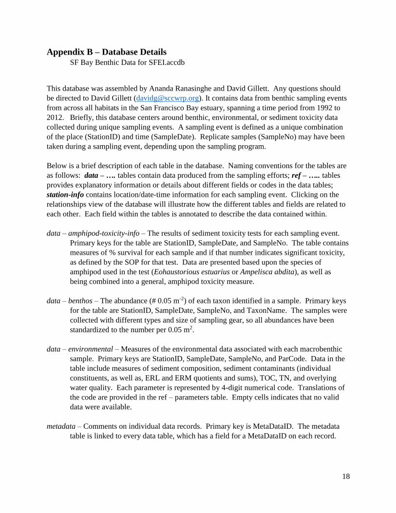
Appendix B – Database Details SF Bay Benthic Data for SFEI.accdb

This database was assembled by Ananda Ranasinghe and David Gillett. Any questions should

be directed to David Gillett ([email protected]). It contains data from benthic sampling events

from across all habitats in the San Francisco Bay estuary, spanning a time period from 1992 to

2012. Briefly, this database centers around benthic, environmental, or sediment toxicity data

collected during unique sampling events. A sampling event is defined as a unique combination

of the place (StationID) and time (SampleDate). Replicate samples (SampleNo) may have been

taken during a sampling event, depending upon the sampling program.

Below is a brief description of each table in the database. Naming conventions for the tables are

as follows: data – …. tables contain data produced from the sampling efforts; ref – ….. tables

provides explanatory information or details about different fields or codes in the data tables;

station-info contains location/date-time information for each sampling event. Clicking on the

relationships view of the database will illustrate how the different tables and fields are related to

each other. Each field within the tables is annotated to describe the data contained within.

data – amphipod-toxicity-info – The results of sediment toxicity tests for each sampling event.

Primary keys for the table are StationID, SampleDate, and SampleNo. The table contains

measures of % survival for each sample and if that number indicates significant toxicity,

as defined by the SOP for that test. Data are presented based upon the species of

amphipod used in the test (Eohaustorious estuarius or Ampelisca abdita), as well as

being combined into a general, amphipod toxicity measure.

data – benthos – The abundance (# 0.05 m-2) of each taxon identified in a sample. Primary keys

for the table are StationID, SampleDate, SampleNo, and TaxonName. The samples were

collected with different types and size of sampling gear, so all abundances have been

standardized to the number per 0.05 m2.

data – environmental – Measures of the environmental data associated with each macrobenthic

sample. Primary keys are StationID, SampleDate, SampleNo, and ParCode. Data in the

table include measures of sediment composition, sediment contaminants (individual

constituents, as well as, ERL and ERM quotients and sums), TOC, TN, and overlying

water quality. Each parameter is represented by 4-digit numerical code. Translations of

the code are provided in the ref – parameters table. Empty cells indicates that no valid

data were available.

metadata – Comments on individual data records. Primary key is MetaDataID. The metadata

table is linked to every data table, which has a field for a MetaDataID on each record.

mailto:[email protected]

19

ref – data sources – A reference table explaining the ProjectCode field: the name of the project

the data were originally collected under and the agency associated with that project.

Primary keys ares SourceAgency and Project. Project details were not available for every

project, so only abbreviations are currently available.

ref – habclass – A reference table explaining each HabClass code associated with each sampling

event in the station-info table. Primary key is HabClass. Habitat descriptions and criteria

are from Ranasinghe et al. (2012) and Thompson et al. (2013).

ref – parameters – A reference table explaining each 4-digit ParCode from the environmental

table. Primary key is ParCode. Units of measure were not available for most of the

parameters.

ref- taxa – A reference table with detailed taxonomic information for each TaxonName in the

data – benthos table. Primary Key is TaxonName.

station-info – A table of station and sampling event information, including number of replicate

samples collected, location, sampling gear, and the source of the data. Primary keys are

StationID and SampleDate. The table also contains information about old station IDs and

old habitat membership.

Documents

Development of Benthic Community Condition … 735 NOV 2014 Development of Benthic Community Condition Indices – San Francisco Bay Contract#: 1038 Phase I Final Report November 26,